Hedge Fund Performance Evaluation under the Stochastic ...zhang654/jfqa2016.pdf · and effective...

JOURNAL OF FINANCIAL AND QUANTITATIVE ANALYSIS Vol. 51, No. 1, Feb. 2016, pp. 231–257COPYRIGHT 2016, MICHAEL G. FOSTER SCHOOL OF BUSINESS, UNIVERSITY OF WASHINGTON, SEATTLE, WA 98195doi:10.1017/S0022109016000120

Hedge Fund Performance Evaluation under theStochastic Discount Factor Framework

Haitao Li, Yuewu Xu, and Xiaoyan Zhang∗

Abstract

We study hedge fund performance evaluation under the stochastic discount factor frame-work of Farnsworth, Ferson, Jackson, and Todd (FFJT). To accommodate dynamic tradingstrategies and derivatives used by hedge funds, we extend FFJT’s approach by consider-ing models with option and time-averaged risk factors and incorporating option returns inmodel estimation. A wide range of models yield similar conclusions on the performance ofsimulated long/short equity hedge funds. We apply these models to 2,315 actual long/shortequity funds from the Lipper TASS database and find that a small portion of these fundscan outperform the market.

I. Introduction

Performance evaluation of actively managed mutual funds and hedge fundsis an important issue facing both finance academics and practitioners. Whethersome actively managed funds can beat the market has important implications forthe efficient market debate. At the same time, identifying funds with superiorperformance is key to the success of investors who must allocate money amongdifferent investment vehicles. Performance evaluation in both theory and prac-tice, however, is challenging because almost all inferences on fund performancedepend on the benchmark models used, leading to the well-known joint hypothe-sis testing problem.

Farnsworth, Ferson, Jackson, and Todd (FFJT) (2002) develop an innovativeand effective approach to mutual fund performance evaluation under the stochas-tic discount factor (SDF) framework. In particular, FFJT examine a wide range ofSDF models using both actual and simulated mutual fund returns. By controllingthe skill levels of the (hypothetical) manager in delivering abnormal returns, FFJT

∗Li, [email protected], Cheung Kong Graduate School of Business, Beijing 100738, China; Xu,[email protected], Fordham University, Gabelli School of Business, New York, NY 10023; andZhang (corresponding author), [email protected], Purdue University, Krannert School of Man-agement, West Lafayette, IN 47906. We thank Andrew Ang, Warren Bailey, Hendrik Bessembinder(the editor), Wayne Ferson (associate editor and referee), and Andrew Karolyi for valuable comments.We thank Jaden Falcone and Steve Sibley for editorial assistance. We are responsible for any remain-ing errors.

231

232 Journal of Financial and Quantitative Analysis

use the simulated fund returns as a benchmark to correct for potential biases ofthe SDF models in evaluating actual mutual fund returns. As a result, FFJT canbetter identify the true skill levels of actual managers and find that the averagemutual fund has enough abnormal performance to cover transaction costs. More-over, they show that except for a few models, a wide variety of SDF models usedin the literature yield similar conclusions on the true ability of managers basedon historical returns, although they tend to have a mild negative bias when trueperformance is neutral.

Although the FFJT (2002) approach works well for mutual funds, the fast-growing hedge fund industry raises new challenges for performance evaluationbecause of the investment strategies and compensation structures of hedge funds.Because hedge funds are not subject to the same level of regulation as mutualfunds, they enjoy greater flexibility in their investment strategies. As a result,they frequently use short selling, leverage, and derivatives, strategies rarely usedby mutual funds, to enhance returns and/or reduce risks. Whereas mutual fundscharge a management fee proportional to assets under management, most hedgefunds charge an incentive fee, typically 15% to 20% of profits, in addition toa fixed management fee of 1% to 2%. Many funds also have a high-watermarkprovision, which requires managers to recoup previous losses before receivingincentive fees. The compensation structure might encourage hedge fund managersto use strategies with option-like payoffs to increase upside potential or to protectdownside risks of their investments.

It has been widely documented in the literature that hedge funds exhibitoption-like returns.1 For example, Fung and Hsieh (2001) show that the returns of“trend-following” funds are highly nonlinear and resemble the returns of “look-back straddles.” Mitchell and Pulvino (2001) show that the returns of “risk ormerger arbitrage” funds have nonlinear exposure to the overall market, withalmost zero beta in up markets and big negative beta in down markets. The mod-els used in FFJT (2002) for mutual fund performance evaluation are mostly linearasset pricing models with stock market factors. As such, these models might notbe directly applicable to hedge funds because of their derivatives usage and non-linear returns. For example, Grinblatt and Titman (1989) show that it would beproblematic for linear asset pricing models to price nonlinear returns.

In this article, we extend the FFJT (2002) approach to study hedge fundperformance evaluation under the SDF framework, which is more suitable thanthe traditional linear regression approach in dealing with nonlinear hedge fundreturns.2 To accommodate dynamic trading strategies and derivatives used byhedge funds, we incorporate both options and time-averaged factors into tradi-tional linear asset pricing models, and use option returns in the estimation of theSDF models. Specifically, we consider a wide range of models, which include the

1TASS, a hedge fund research company, reports that more than 50% of the 4,000 hedge fundsit follows use derivatives. Merton (1981), Dybvig and Ross (1985), and others show that dynamictrading strategies could generate option-like returns. For empirical evidence, see, for example, Fungand Hsieh (1997), Agarwal and Naik (2004), and Ben Dor, Jagannathan, and Meier (2003).

2See Cochrane (2005) for a comprehensive treatment of theoretical and empirical asset pricingbased on the SDF approach.

Li, Xu, and Zhang 233

unconditional and conditional versions of the capital asset pricing model (CAPM),the Fama–French (1993) model augmented by the momentum factor, the modelof Agarwal and Naik (2004) with two option factors, and the 7-factor model ofFung, Hsieh, Naik, and Ramadorai (FHNR) (2008).3 Following Ferson, Henry,and Kisgen (2006) and Patton and Ramadorai (2013), we consider models withtime-averaged factors to account for interim trading of hedge funds. We also applythe approach of Getmansky, Lo, and Makarov (2004) to control for potential biasin hedge fund returns due to stale prices and illiquid holdings. The FFJT (2002)approach provides a common platform to systematically study the abilities ofthese models in identifying the true performance of hedge funds. We estimateall the SDF models using stock and option returns as primitive test assets, ensur-ing that the estimated models are consistent with derivatives pricing. We find thatsome of the SDF models can price the 16 primitive test assets reasonably well. Infact, certain SDF models cannot be rejected by the Hansen–Jagannathan (1997)specification test.

We apply the SDF models to the simulated returns of long/short equity hedgefunds, whose managers have known abilities in delivering abnormal returns. Wefocus on long/short equity funds because they represent the largest number ofhedge funds and have one of the largest assets under management among allhedge fund strategies in the past two decades. Specifically, we assume that a man-ager receives signals about the CAPM residuals of the 1,000 largest stocks in theCenter for Research in Security Prices (CRSP). The manager would long (short)the stocks with a signal that is better (worse) than the average signal of all stocks.A skilled manager receives signals with higher precision and thus can deliverhigher alphas. Applying the SDF models to the simulated hedge fund returns, wefind that most models yield similar conclusions on the abnormal performance withreasonable accuracy. Most models have a slight negative bias when the managerhas no ability to deliver positive alpha, which is similar to the findings of FFJT(2002) for mutual funds.

Finally, we apply the SDF models to the monthly net-of-fee returns of 2,315actual long/short equity funds covered by TASS, a comprehensive data set onhedge funds. Simple regression analysis shows that about 58% of the long/shorthedge funds have nonlinear exposure to either the market factor or option factors.The simulated hedge fund returns display nonlinearity similar to those observedin the actual hedge fund returns. We compare the distribution of the alphas ofthe 2,315 actual hedge funds under each SDF model with those of the simulatedhedge funds. We find that most hedge funds cannot beat the market, in the sensethat their alphas are comparable to those of the simulated funds with low-skilledmanagers. However, a small portion of these hedge funds do seem to be able tooutperform the market, with alphas similar to those of the simulated hedge fundswith highly skilled managers. Our results show that the general approach of FFJT(2002) is equally applicable to hedge fund performance evaluation.

3Agarwal and Naik (2004) include option returns as factors in traditional asset pricing modelsto capture nonlinear hedge fund returns. Fung and Hsieh (2001) propose a 7-factor model, which, inaddition to traditional stock, bond, and credit market factors, includes excess returns of portfolios oflookback straddles on currencies, commodities, and bonds.


The remainder of this article is organized as follows: In Section II, wediscuss hedge fund performance evaluation under the SDF framework of FFJT(2002). In Section III, we apply a wide range of SDF models to the simulatedreturns of long/short equity hedge funds with managers of known abilities in de-livering abnormal returns. We discuss the data in Section IV and provide empir-ical evidence on the performance of the 2,315 long/short equity hedge funds inSection V. Section VI concludes the article.

II. Hedge Fund Performance Evaluation under the SDFFramework

In this section, we first introduce the SDF approach of FFJT (2002) for per-formance evaluation. We then discuss the unique features of hedge fund returnsand the SDF models used for hedge fund performance evaluation.

A. The SDF Approach of FFJT

Although the existing literature on mutual fund performance heavily relieson linear asset pricing models, FFJT (2002) is one of the first studies that ex-amines performance evaluation under the general and flexible SDF framework.The fundamental theorem of asset pricing, one of the cornerstones of neoclassi-cal finance, establishes the equivalence between the existence of a positive SDFthat correctly prices all primitive test assets and the absence of arbitrage. Supposewe have n primitive test assets with gross returns Rt (an n × 1 vector) at t fort = 0, 1, . . . ,T . Then for all t, we must have

E [mtRt|Ft−1] = 1n×1,(1)

where 1n×1 is an n × 1 vector of ones, Ft−1 denotes the information set availableat time t − 1, and E [·|Ft−1] denotes the conditional expectation given Ft−1. Thescalar random variable mt discounts total payoffs at t state by state to yield the“present value” at t − 1, which is equal to $1.

For the purpose of performance evaluation, we need to identify a particularSDF, mt, which can price all the primitive test assets and thus satisfy equation (1).Then we can use the SDF model to evaluate the performance of actively man-aged funds. Because it is practically infeasible to include all public informationin the empirical estimation of equation (1), the empirical asset pricing literaturetypically uses predetermined information variables, Zt−1, which are elements ofthe public information set Ft−1. By the law of iterated expectations, equation (1)holds when we replace Ft−1 with Zt−1:

E [mtRt|Zt−1] = 1n×1.(2)

A conditional approach to performance evaluation allows a researcher to set thestandard for what is “superior” information by choosing the public informationZt−1. When Zt−1 is restricted to be a constant, we have an unconditional measure.

An asset pricing model proposes an SDF, yt, as a proxy for the true SDF, mt.In this article, we define yt as a function of risk factors and prices of risks:

yt = f (b,Ft),(3)


where b is a k × 1 vector of prices of risks, Ft is a k × 1 vector of risk factors,and f (·) is the functional form of yt. Similar to FFJT (2002), we define the pricingerror of a given yt as:

αt = E [ytRt|Zt−1]− 1,(4)

which measures the difference between the price of Rt implied by yt and the trueSDF, mt. If yt prices the primitive assets correctly, then αt should be 0 for all theprimitive assets and their linear combinations.

We estimate the parameters of yt (i.e., the prices of risks, b) by minimizingthe Hansen–Jagannathan (1997) distance (HJ-distance hereafter), which is definedas:

δ =√E(α′)E−1(RR′)E(α).

The HJ-distance is similar to the generalized method of moments (GMM) objec-tive function when the pricing error, α, is used as the moment condition. WhereasGMM uses the optimal weighting matrix, the HJ-distance uses E

−1(RR′) as theweighting matrix. Because E

−1(RR′) is the same across different models, it iseasier to compare model performance based on the HJ-distance. The HJ-distancealso has a nice economic interpretation as the maximum pricing error of all lin-ear payoffs constructed from the primitive assets, Rt, with an unit norm. Thismakes model comparison based on the HJ-distance economically meaningful. Inaddition to estimating model parameters and pricing errors, we conduct modelspecification tests based on the HJ-distance. In short, the HJ-distance allows us toselect the best model for hedge fund performance evaluation given its ability toprice the primitive test assets.4

B. SDF Models for Hedge Fund Performance Evaluation

One of the challenges for hedge fund performance evaluation is that hedgefunds tend to exhibit nonlinear, option-like returns because of their flexible trad-ing strategies.5 We extend the FFJT (2002) approach in three important dimen-sions to deal with the unique features of hedge fund returns. First, we considerSDF models with nonlinear risk factors constructed from option returns. For in-stance, we consider the model of Agarwal and Naik (2004) with 2 option factorsthat capture the volatility and jump risks in the index option market. Second,following Ferson et al. (2006) and Patton and Ramadorai (2013), we constructtime-averaged monthly risk factors using averages of daily factors to account forinterim trading and derivatives used by hedge funds. Finally, we include indexoption returns as primitive test assets in model estimation to ensure that the SDFmodels can capture the major risk factors in index option returns.

We first consider the unconditional CAPM as in Sharpe (1964):

yCAPMt = b0 + b1MKTt,(5)

4Detailed discussions on how to use HJ-distance to systematically compare models can be foundin Li, Xu, and Zhang (2010).

5We present more evidence on nonlinear hedge fund returns in the data section.


where MKTt represents the monthly excess return of the market portfolio, proxiedby the monthly return of the value-weighted CRSP index in excess of the 1-monthrisk-free rate. To allow time-varying prices of risks, we consider a conditionalversion of the CAPM with a conditioning variable, zt−1:

yCAPMIVt = (b0 + b1zt−1) + (b2 + b3zt−1)MKTt.(6)

The above two models ignore within-month variations in the risk factors. Next, weconsider models with time-averaged factors, using information from daily data.For brevity, we discuss only conditional models with time-averaged factors.6 Forthe conditional CAPM, the pricing model is specified as:

yCAPMIVDt = b0 + b1zD,t−1 + b2MKTD,t + b3ZMKTD,t,(7)

where zD,t−1 is the average of daily observations of the conditioning variable formonth t − 1, MKTD,t is the average of daily observations of MKT for montht, and ZMKTD,t is the average of the product of the daily conditioning variable(from month t − 1) and daily MKT for month t. We use the superscript “D” todenote models with daily averaged factors.

To capture the cross-sectional patterns in stock returns due to size, value,and momentum effects, we consider the Fama–French (1993) 3-factor model aug-mented by the momentum factor with the following SDF:

yFFt = b0 + b1MKTt + b2SMBt + b3HMLt + b4MOMt,(8)

where SMBt, HMLt, and MOMt are the return differentials between small andlarge firms, high and low book-to-market firms, and winner and loser firms,respectively.7 The conditional version of this model (denoted as FFIV), whichis considered by Kirby (1997), has the following SDF:

yFFIVt = (b0 + b1zt−1) + (b2 + b3zt−1)MKTt + (b4 + b5zt−1)SMBt(9)

+ (b6 + b7zt−1)HMLt + (b8 + b9zt−1)MOMt.

We also consider an alternative conditional Fama–French (1993) model (denotedas FFIVD) with time-averaged factors,

yFFIVDt = (b0 + b1zD,t−1) + (b2MKTD,t + b3ZMKTD,t)(10)

+ (b4SMBD,t + b5ZSMBD,t) + (b6HMLD,t + b7ZHMLD,t)

+ (b8MOMD,t + b9ZMOMD,t),

where ZSMBD,t, ZHMLD,t, and ZMOMD,t are computed in a similar way asZMKTD,t.

To capture the option-like returns of hedge funds, Agarwal and Naik (2004)consider risk factors constructed from option returns. Similarly, we consider anoption-based model, OPT,

yOPTt = b0 + b1MKTt + b2STRt + b3SKEWt,(11)

6We thank the referee for the suggestion of considering interim trading and time-averaged factors.7All factors of the Fama–French (1993) model are obtained from Kenneth French’s Web site

(http://mba.tuck.dartmouth.edu/pages/faculty/ken.french/data library.html).


where we incorporate two additional factors from the option market into theCAPM. The first factor, STRt, is the return on at-the-money (ATM) Standard& Poor’s (S&P) 500 index straddles with time to maturity between 20 and 50days. This factor captures the aggregate volatility risk as in Ang, Hodrick, Xing,and Zhang (2006). The second factor, SKEWt, is the return on out-of-the-money(OTM) S&P 500 index puts that expire in 20 to 50 days. This factor capturesjump risk in the market index. The data for option returns are obtained fromOptionMetrics. The conditional version of the option-based model is specified as:

yOPTIVt = (b0 + b1zt−1) + (b2 + b3zt−1)MKTt(12)

+ (b4 + b5zt−1)STRt + (b6 + b7zt−1)SKEWt.

The time-averaged version of OPT is specified as:

yOPTIVDt = (b0 + b1zD,t−1) + (b2MKTD,t + b3ZMKTD,t)(13)

+ (b4STRD,t + b5ZSTRD,t) + (b6SKEWD,t + b7ZSKEWD,t),

where ZSTRD,t and ZSKEWD,t are computed in a similar way as ZMKTD,t.The 7-factor model of FHNR (2008) combines option factors with equity

factors and has the following SDF:

yFHNRt = b0 + b1MKTt + b2SMBt + b3FXSTRt(14)

+ b4COSTRt + b5BDSTRt + b6TERMt + b7DEFt,

where the three option factors are constructed from returns of lookback straddlesfor currencies (FXSTR), commodities (COSTR), and bonds (BDSTR). FHNRalso include SMB, TERM (the yield spread between 10-year Treasury bond and3-month Treasury bill (T-bill)), and DEF (changes in the credit spread betweenMoody’s BAA bond and 10-year Treasury bond) as risk factors. The conditionalFHNR model is specified as:

yFHNRIVt = (b0 + b1zt−1) + (b2 + b3zt−1)MKTt + (b4 + b5zt−1)SMBt(15)

+ (b6 + b7zt−1)FXSTRt + (b8 + b9zt−1)COSTRt

+ (b10 + b11zt−1)BDSTRt + (b12 + b13zt−1)TERMt

+ (b14 + b15zt−1)DEFt.

We do not consider a time-averaged version of FHNR because we do not havedaily returns of the look-back straddles.

Finally, we introduce a new model as an alternative to FHNR (2008) tocapture nonlinearities in hedge fund returns. The new model, MIX, mixes theoption-based model with the Fama–French (1993) model and has the followingSDF:

yMIXt = b0 + b1MKTt + b2SMBt + b3HMLt(16)

+ b4MOMt + b5STRt + b6SKEWt.

The factors of the conditional versions of MIX, MIXIV, and MIXIVD are allscaled by the conditioning variables. Whereas the FHNR model has been devel-oped mainly for trend-following funds, our MIX model might be more appropriatefor funds that mainly invest in equities and equity derivatives.


The previous literature has suggested three widely used conditioning vari-ables: 1-month T-bill rate, TERM, and DEF. Because both TERM and DEF havebeen included as risk factors in the FHNR (2008) model, we use the 1-monthT-bill rate to scale the risk factors to obtain time-varying market prices of risks.We use TERM and DEF to scale the returns of the primitive test assets to approx-imate the returns of dynamic trading strategies. We require the SDF models toprice both the unscaled and scaled returns of the primitive test assets.

III. Simulated Hedge Fund Returns

To test whether the SDF models can accurately evaluate hedge fund perfor-mance, following FFJT (2002), we apply them to simulated hedge fund returnswith managers of known abilities in delivering abnormal returns. The simulatedhedge fund returns can then serve as a benchmark for evaluating actual hedge fundperformance. For example, we can identify the skill levels at which the simulatedreturns are comparable to the actual returns.

We obtain simulated returns of an artificial long/short equity hedge fundbased on the actual returns of the 1,000 largest stocks from CRSP betweenJan. 1996 and Dec. 2012, the period for which we have actual hedge fund data.We assume that each month the manager receives a signal about the CAPM resid-ual of each of the 1,000 stocks.8 The manager would long (short) the stocks witha signal that is better (worse) than the average signal of all the stocks. A moreskilled manager would receive a signal with higher precision and thus can deliverhigher abnormal returns on average.

Specifically, we assume that the returns of the 1,000 stocks follow the CAPMrelation:

rit = αi + βirmt + εit,(17)

where for each month t, rit is the excess return of stock i, rmt is the excess returnof the market portfolio, εit is the idiosyncratic component of the stock return, andαi and βi are the intercept and slope coefficients of the CAPM regression, respec-tively. We assume that at the beginning of each month t, the manager receives asignal, sit, and

sit = γεit + (1 − γ)σiuit,(18)

where uit represents the noise in the signal and follows an independent and iden-tically distributed standard normal distribution, σi measures the full-sample time-series volatility of εit for each firm i, and γ (between 0 and 1) measures the skilllevel of the manager.9 A higher γ means that the manager has a more precisesignal about εit. Suppose γ = 1, then at the beginning of month t, the managerwould know whether rit would out- or underperform the market based on his or

8We also consider residuals from nonlinear models other than the CAPM and obtain similarresults, which are available from the authors.

9We also allow the firm-level idiosyncratic volatility to be time varying and estimate σi using a24-month rolling window. We obtain similar results, which are available from the authors.


her signal on εit. The manager then can long or short the stock based on εit andearn abnormal returns.10

We define st = 1/N∑N

i=1 sit as the average level of the original signal acrossthe 1,000 stocks at time t, with N = 1,000. We assume that the manager longsthe stocks with above-average signals and shorts the stocks with below-averagesignals. Our weights are similar to those used in Khandani and Lo (2011), whoalso simulate returns on long/short equity hedge funds. To be more specific, forfirms with positive signals, the weights are defined as:

w+it =

(sit − st) I+it∑N

i=1 (sit − st) I+it

, I+it = 1 if sit > st, and 0 otherwise.(19)

Similarly, for firms with negative signals, the weights are defined as:

w−it = − (sit − st) I−it∑N

i=1 (sit − st) I−it, I−it = 1 if sit < st, and 0 otherwise.(20)

The portfolio is self-financing, because the weights sum to 0:

N∑i=1

(w+it + w−

it ) = 1 − 1 = 0.(21)

Based on the weights above, the return on the long/short portfolio at tbecomes

rp =N∑

i=1

(w+it + w−

it )rit = αpt + βptrmt + εpt,(22)

where αpt ∝ ∑Ni=1 (sit − st)αi, βpt ∝ ∑N

i=1 (sit − st)βi, and εpt ∝∑Ni=1 (sit − st) εit. We emphasize that the signal is about the idiosyncratic compo-

nent of the return of each stock. Even though the stock might have a zero α, a man-ager with a relatively accurate signal can still beat the market, because E(εpt|st)could be nonzero. Moreover, a more accurate signal will lead to higher corre-lation between portfolio weights and subsequent realized idiosyncratic returns,which will lead to higher excess returns for the portfolio.

Although sit is a signal about the magnitude of εit, in reality investors mightwant to adjust the original signal by return variances to maximize the informationratio or Sharpe ratio of their investments. Therefore, we also consider a mod-ified signal, s∗it = sit/σ

2i , where the original signal is scaled by the variance of

the residual.11 The derivation for the scaled signal is provided in the Appendix.When the signals are scaled by return variances, the resulting weights still followequations (19) and (20), except sit should be replaced by s∗it. In the later empiricalsection, we present results for both the original and the scaled signals.

10One way to understand the implications of different levels of γ is to regress sit on εit. When γincrease from 0.1 to 0.2, the average R2 of the above regression increases from 1% to 4%. When γbecomes 0.5 (0.9), the average R2 becomes 41% (98%). Therefore, a higher γ means that the managerhas a more precise estimation of εit .

11We thank the referee for suggesting this alternative signal.


Although in theory the long/short portfolio has 0 net investment, in realityone must put down money to initiate both the long and short positions. Mean-while, a manager with a positive γ can generate positive abnormal returns, whichcan be further magnified by leverage. The Federal Reserve Board Regulation Tallows a maximum leverage ratio of 2:1.12 About 60% of the 2,315 long/shortequity funds in TASS report usage of leverage with an average leverage ratio ofabout 2:1. In our simulation analysis, we consider two cases: a conservative lever-age ratio of 1:1 and a more aggressive leverage ratio of 2:1 as in Khandani and Lo(2011).

IV. The Data

Our empirical analysis mainly relies on monthly observations of the follow-ing four types of data between Jan. 1996 and Dec. 2012: i) risk factors for theSDF models, ii) conditioning variables used to capture time-varying prices ofrisks and/or dynamic trading strategies, iii) returns of primitive test assets used inestimating the SDF models, and iv) returns of 2,315 long/short equity hedge fundsfrom TASS. Table 1 provides the mean, standard deviation, minimum, maximum,and autocorrelation for all the data items used in our analysis.

Panel A of Table 1 provides summary information of the risk factors andthe conditioning variables. The first four factors, MKT, SMB, HML, and MOM,are standard stock market factors widely used in the current asset pricing litera-ture and all exhibit positive means and sizable volatilities. The two option factorsfrom Agarwal and Naik (2004), STR and SKEW, capture the volatility and jumprisk premiums in the index option market. Consistent with the well-known resultsin the option pricing literature, the straddle factor earns a negative risk premium.The other three option factors from FHNR (2008), FXSTR, COSTR, and BDSTR,capture the returns of look-back straddles on currencies, commodities, and bonds,respectively. Their summary statistics are very similar to those in FHNR. Thethree conditioning variables, RF (the 1-month T-bill rate), TERM, and DEF, areall highly persistent and exhibit strong autocorrelations. To account for poten-tial bias in statistical inference due to these persistent conditioning variables, alltest statistics on the pricing errors (including the HJ-distance test) are based onNewey–West (1987) adjusted standard errors.13

Panel B of Table 1 reports the summary statistics of the primitive test assetsused in our estimation of the SDF models. These assets represent the investmentopportunity set available to hedge fund managers and have enough return spreadsto differentiate candidate SDF models. We first consider 6 stock portfolios sortedby size and book-to-market ratio to capture cross-sectional return differences dueto the size and value effects documented in Fama and French (1993). We also con-sider 6 stock portfolios sorted by size and past returns. The latter represents the

12Leverage is defined as the ratio between the total absolute long and short positions and the capitalinvolved in establishing the long and short positions. For example, if the fund has established $100long and $100 short positions with $100 capital, then the leverage ratio would be 2:1.

13Ferson, Sarkissian, and Simin (2008) show that previous studies have overstated the significanceof time-varying alphas in models with persistent predictors multiplied by contemporaneous factors.Although we do not have time-varying alphas, we minimize possible biases due to persistent condi-tioning variables by using Newey–West (1987) adjusted standard errors.


TABLE 1

Summary Statistics

Table 1 provides summary statistics on all the data items used in our empirical analysis. The sample period is betweenJan. 1996 and Dec. 2012, which yields 204 months of observations. Panel A reports monthly summary statistics for riskfactors and conditioning variables. The first 4 factors, MKT, SMB, HML, and MOM, are standard stock market factors. The 2option factors, STR and SKEW, capture the volatility and jump risk premiums in the index option market. The other 3 optionfactors, FXSTR, COSTR, and BDSTR, capture the returns of lookback straddles on currencies, commodities, and bonds,respectively. The 3 conditioning variables are RF (1-month Treasury bill rate), TERM spread (yield difference between10-year and 3-month Treasury bonds), and DEF spread (yield difference between Baa and Aaa corporate bonds). Panel Bincludes monthly summary statistics for 15 primitive assets. The first 6 stock portfolios are sorted by size and book-to-market ratio (BM). The second 6 stock portfolios are sorted by size and past returns. The last 3 primitive assets areat-the-money (ATM) calls, ATM puts, and out-of-the-money (OTM) puts on the S&P 500 index. Panel C reports monthlysummary statistics of 2,315 long/short equity hedge funds from TASS. Panel D reports nonlinearities in hedge fund returns.The 2,315 hedge fund returns are regressed on 2 sets of factors. The first regression includes MKT, MKT2, and MKT3,whereas the second includes MKT, STR, and SKEW. We report the mean, standard deviation, and percentage of theregression coefficients that are statistically significant.

Factors Mean Std Dev Minimum Maximum Rho

Panel A. Summary Statistics of the Risk Factors and Conditioning Variables

MKT 0.0047 0.0476 −0.1723 0.1134 0.1173SMB 0.0025 0.0366 −0.1639 0.2200 −0.0794HML 0.0028 0.0348 −0.1260 0.1384 0.1160MOM 0.0043 0.0570 −0.3474 0.1839 0.0750STR −0.3254 0.7252 −1.3384 2.9177 −0.0339SKEW −0.3664 0.8804 −0.9792 5.1544 0.1222FXSTR −0.0193 0.1511 −0.2663 0.6886 0.1109COSTR −0.0034 0.1857 −0.3000 0.6922 0.0365BDSTR −0.0001 0.1396 −0.2465 0.6475 −0.0287

RF 0.0023 0.0018 0.0000 0.0056 0.9791TERM 0.0199 0.0137 −0.0023 0.0415 0.9886DEF 0.0102 0.0047 0.0055 0.0338 0.9623

Assets Mean Std Dev Minimum Maximum Rho

Panel B. Summary Statistics of the Returns of the Primitive Test Assets

Small low BM 0.0066 0.0747 −0.2436 0.2816 0.0898Small med BM 0.0111 0.0564 −0.1928 0.1668 0.1286Small high BM 0.0121 0.0593 −0.2030 0.1806 0.1981

Big low BM 0.0073 0.0471 −0.1505 0.1018 0.0715Big med BM 0.0077 0.0477 −0.1731 0.1260 0.1485Big high BM 0.0073 0.0522 −0.2254 0.1627 0.1726

Small low MOM 0.0080 0.0868 −0.2566 0.4632 0.1905Small med MOM 0.0104 0.0539 −0.2073 0.2202 0.1736Small high MOM 0.0128 0.0662 −0.2062 0.2695 0.0802

Big low MOM 0.0051 0.0716 −0.2390 0.3421 0.1429Big med MOM 0.0068 0.0437 −0.1564 0.1389 0.0896Big high MOM 0.0088 0.0491 −0.1489 0.1248 0.0737

ATM call −0.0804 0.8182 −0.9839 2.8548 0.0477ATM put −0.2450 0.8607 −0.9424 3.8962 0.1201OTM put −0.3664 0.8804 −0.9792 5.1544 0.1222

Hedge FundReturns Mean Std Dev Minimum Maximum Rho

Panel C. Summary Statistics of the Returns of the 2,315 Long/Short Equity Hedge Funds

Lower 25% −0.0001 0.0526 −0.9015 1.1640 0.139625% to 50% 0.0057 0.0418 −0.8000 0.8850 0.127759% to 75% 0.0092 0.0505 −0.6541 0.7693 0.1359Top 25% 0.0169 0.0767 −0.9586 2.7286 0.0273

Independent % ofRegression Variable Mean Std Dev Significance

Panel D. Nonlinearities of Hedge Fund Returns

1 MKT 0.5395 1.7103 70%1 MKT2 −0.0048 0.1773 16%1 MKT3 −0.0031 0.1204 26%

2 MKT 0.5475 1.6776 50%2 STR −0.0032 0.0361 26%2 SKEW 0.0031 0.0645 29%


winner and loser portfolios and thus captures the momentum effect of Jegadeeshand Titman (1993). The 12 stock portfolios cover the most popular investmentstyles for equity investors. Next, we include returns of ATM calls, ATM puts, andOTM puts on the S&P 500 index, which are among the most widely traded optionsin the world. Finally, we include the 1-month risk-free rate to anchor the mean ofthe SDF models. Panel B reports the summary statistics of the first 15 test assets,whereas the 1-month risk-free rate is summarized in Panel A of Table 1. Consis-tent with the existing literature, we find that value firms have higher returns thangrowth firms and winner firms have higher returns than loser firms. Compared tostock returns, option returns have much higher means and volatilities.

The hedge fund data used in our analysis are obtained from TASS, which isprobably the most comprehensive data set used in the current hedge fund litera-ture. The data set covers more than 4,000 funds from Nov. 1977 to Dec. 2012,which are classified into “live” and “graveyard” funds. The graveyard databasedid not exist before 1994. To mitigate the problem of survivorship bias, we con-sider both live and graveyard funds and restrict our sample to the period betweenJan. 1996 and Dec. 2012. The database provides monthly net-of-fee returns andnet asset values for each fund.

The hedge funds covered by TASS follow 11 investment styles and trade ina wide range of markets. Therefore, it is difficult to replicate the trading strategiesand derivatives used by every hedge fund strategy. We focus on long/short equityhedge funds because they cover the largest number of hedge funds in TASS andhave one of the largest group of assets under management during our sampleperiod.14 Specifically, we have 2,315 long/short equity hedge funds in TASS.

Panel C of Table 1 reports the distribution of the summary statistics for 4quartiles of the net-of-fee monthly returns of the 2,315 hedge funds. We see thatthe mean monthly returns range from −0.01% in the lowest quartile to 1.69% inthe highest quartile, and the standard deviation increases from 5.26% to 7.67%.Panel D highlights the exposure of hedge fund returns to nonlinear market fac-tors and option factors. We consider two regressions of individual hedge fundreturns. In the first regression, the independent variables include the market factorand its second and third moments. In the second regression, we include the mar-ket, straddle, and skewness factors. In both regressions, we find that about 60%to 70% of hedge funds have significantly nonzero loadings on the market factor,which means that these funds are not exactly market neutral. About 16% (26%)of the hedge funds have significant nonzero exposures to the second (third) mo-ment of the market factor. About 26% (29%) of the hedge funds have significantnonzero exposures to the straddle (skewness) factors. Collectively, about 58% ofthe long/short hedge funds have significant exposures to at least one of the non-linear factors constructed on the market portfolio.15

One common interpretation of nonlinearity in fund returns is that it reflectsmarket-timing ability of managers. Treynor and Mazuy (1966) provide theclassical connection between market timing and nonlinearity. Chen, Ferson, and

14The total asset under management in the long/short category reported in TASS is about $170billion as of 2012.

15This number can not be deduced directly from Panel D of Table 1 because many stocks havesignificant exposures to multiple nonlinear factors.


Peters (2010) consider the issue of identifying true market-timing ability and ex-amine different categories of biases that lead to nonlinearity. After controlling forthese biases, the authors find positive evidence of market-timing ability for bondfund managers. A more recent paper by Cao, Chen, Liang, and Lo (2013) showsthat hedge fund managers can even time market liquidity. In fact, FFJT (2002)consider a separate simulation design just to mimic the market-timing ability ofmutual fund managers. The nonlinearity we observe in hedge fund returns couldbe due to market timing by hedge fund managers or nonlinear exposures of thestocks held by the funds. In results not reported here, we find that the returns ofroughly 30% of the 1,000 stocks in our sample have significant loadings on thenonlinear factors. This suggests that the nonlinearity in hedge fund returns couldbe driven by the nonlinearity in the returns of the stocks they hold. Although wedo not rule out the possibility that hedge fund managers could time the market, inour simulation and empirical analysis, we focus on stock picking, which is likelythe most important source of alpha and one of the main appeals of long/shortequity hedge funds.

V. Empirical Results on Hedge Fund PerformanceEvaluation

In this section, we provide empirical analysis of the performance of the 2,315long/short equity hedge funds using the SDF approach. First, we estimate all theSDF models using the 16 primitive test assets and identify models that can pricethe test assets well. Second, we apply the SDF models to evaluate simulated hedgefund returns to gauge their power to detect abnormal performance when the abilityof the manager is known. Finally, we apply the SDF models to evaluate the returnsof the 2,315 long/short equity hedge funds, using the results for the simulatedreturns as a benchmark to adjust for potential biases in the SDF models.

A. Estimating the SDF Models

Table 2 reports the empirical results on the estimation of the SDF models.Panel A contains the results based on the returns of the 16 primitive test assets.Panels B and C contain the results based on the returns of the primitive assetsscaled by TERM and DEF, respectively. In each panel, we report the estimatedHJ-distance, the asymptotic p-values of the specification test based on theHJ-distance, as well as p-values based on the finite-sample empirical distributionof the HJ-distance to correct for potential biases in the asymptotic distribution.16

We also report the mean, standard deviation, minimum, and maximum of each

16Previous studies (e.g., Ferson and Foerster (1994)) show that asymptotic tests based on 2-stageGMM estimation tend to overreject the null hypothesis. Ahn and Gadarowski (2004) find similaroverrejection problem for the HJ-distance estimation. To correct the overrejection bias, our empiricalp-values are estimated from 5,000 simulations. For each simulation, we first generate returns by usingmodel-implied expected returns with normally distributed noises. That is, from the pricing equationE(yr) = p, under the null, E(r) = [p − cov(y, r)]/E(y). Next, we estimate the HJ-distance for eachsimulated sample of returns. The empirical p-values are calculated as percentages of HJ-distancesestimated over simulations that are bigger than the HJ-distance estimated from real data.


TABLE 2

Estimation of the SDF Models Based on the 16 Primitive Test Assets

Table 2 reports the empirical results of the estimation of the stochastic discount factor (SDF) models. Our sample periodis from Jan. 1996 to Dec. 2012, with 204 monthly observations. Panel A contains the results based on the returns of the16 primitive test assets. Panels B and C contain the results based on the scaled returns of the primitive assets by termpremium (TERM) and default premium (DEF), respectively. In each panel, we report the estimated Hansen–Jagannathan(1997) distance (HJ-Dist) of each model, as well as the mean, standard deviation, minimum, and maximum of eachestimated SDF model. We report the asymptotic and empirical p-values of the specification test based on the HJ-distancefor all the SDF models.

HJ-Dist EmpiricalSDF Models d p(d = 0) p(d = 0) Mean Std Dev Min Max

Panel A. Estimation of the SDF Models Based on the Returns of the Primitive Assets

CAPM 0.985 0% 0% 0.998 0.103 0.762 1.380CAPMIV 0.978 0% 0% 0.998 0.210 0.452 1.963CAPMIVD 0.969 0% 0% 0.998 0.305 0.241 2.429

FF 0.967 0% 0% 0.998 0.216 0.437 1.863FFIV 0.780 2% 0% 0.997 2.039 −4.052 9.788FFIVD 0.681 21% 8% 0.998 2.643 −6.284 12.159

OPT 0.773 0% 6% 0.998 0.623 −0.597 5.172OPTIV 0.699 19% 12% 0.999 1.762 −4.268 10.498OPTIVD 0.525 6% 86% 0.998 1.701 −13.687 9.439

FHNR 0.805 1% 0% 0.998 1.357 −2.050 5.659FHNRIV 0.000 0.980 23.537 −56.808 99.977

MIX 0.733 0% 6% 0.998 0.671 −0.889 5.465MIXIV 0.351 45% 37% 0.998 4.026 −11.893 17.987MIXIVD 0.185 68% 82% 1.000 2.837 −17.176 10.854

Panel B. Estimation of the SDF Models Based on the Returns of the Primitive Assets Scaled by TERM

CAPM 0.913 0% 0% 0.997 0.125 0.713 1.459CAPMIV 0.339 6% 100% 0.995 1.469 −1.224 4.311CAPMIVD 0.339 5% 100% 0.995 1.466 −1.201 4.238

FF 0.896 0% 0% 0.997 0.268 −0.564 1.994FFIV 0.192 61% 100% 0.995 2.124 −5.334 12.112FFIVD 0.185 79% 100% 0.995 2.227 −5.778 10.088

OPT 0.832 0% 1% 0.997 0.529 −0.212 4.690OPTIV 0.315 3% 100% 0.995 1.599 −2.208 4.886OPTIVD 0.259 23% 100% 0.995 1.773 −1.540 7.949

FHNR 0.693 0% 57% 0.996 1.509 −4.195 5.292FHNRIV 0.000 89% 0.995 2.702 −6.201 6.880

MIX 0.804 0% 1% 0.997 0.602 −0.821 5.228MIXIV 0.104 66% 95% 0.995 2.625 −8.788 10.553MIXIVD 0.102 79% 95% 0.995 2.747 −8.261 13.394

Panel C. Estimation of the SDF Models Based on the Returns of the Primitive Assets Scaled by DEF

CAPM 1.001 0% 0% 0.997 0.071 0.836 1.260CAPMIV 0.831 0% 5% 0.995 1.606 −1.285 3.621CAPMIVD 0.832 0% 2% 0.995 1.583 −1.125 4.016

FF 0.986 0% 0% 0.997 0.199 0.409 1.781FFIV 0.511 31% 52% 0.994 2.854 −5.656 10.991FFIVD 0.473 42% 62% 0.994 2.854 −6.029 12.924

OPT 0.838 0% 0% 0.997 0.611 −0.570 5.010OPTIV 0.701 0% 8% 0.995 1.717 −3.061 4.633OPTIVD 0.547 1% 60% 0.997 1.788 −13.650 10.053

FHNR 0.774 0% 5% 0.997 1.389 −2.248 6.120FHNRIV 0.000 46% 0.993 6.306 −13.452 20.826

MIX 0.807 0% 0% 0.997 0.652 −0.965 5.321MIXIV 0.404 9% 22% 0.995 3.000 −8.430 13.742MIXIVD 0.223 58% 67% 0.997 3.619 −12.920 12.483

estimated SDF model, yt. Because the results in Panels B and C based on thescaled returns of the primitive assets are similar to those in Panel A, we focus ourdiscussion on the results in Panel A.17

17We also consider exponential models in addition to linear models. The advantage of exponen-tial models is that they will always be nonnegative and thus do not allow arbitrage opportunities.


Among the unconditional models, the CAPM has the highest HJ-distance(0.985), followed by FF (0.967), FHNR (0.805), OPT (0.773), and MIX (0.733).The fact that MIX has smaller HJ-distance than FHNR highlights the importanceof the three stock market factors (SMB, HML, and MOM) and the two optionfactors (STR and SKEW) for pricing the primitive test assets. All the condi-tional models using monthly information (CAPMIV, FFIV, OPTIV, FHNRIV, andMIXIV) have much smaller HJ-distances than their unconditional counterparts.FHNRIV has a 0 HJ-distance, because with 16 parameters it can fit 16 assets per-fectly. The models with time-averaged factors (CAPMIVD, FFIVD, OPTIVD,and MIXIVD) have even smaller HJ-distances than the models with monthlyfactors, highlighting the importance of considering interim trading and within-month variations.

All the unconditional models except FHNR (2008) are overwhelminglyrejected by the specification test based on the HJ-distance with 0 asymptoticp-values. Using the empirical p-values based on finite-sample simulations, whichare generally larger than asymptotic p-values, we cannot reject the null hypothesisthat OPT and MIX are correctly specified at the 5% confidence level (the empir-ical p-values are 6%). The asymptotic p-values of the specification test basedon the HJ-distance for the four conditional models with monthly information,CAPMIV, FFIV, OPTIV, and MIXIV, are 0%, 2%, 19%, and 45%, respectively.The p-values of the conditional models with time-averaged factors are mostlyhigher than those with monthly factors. However, it should be noted that the con-ditional models tend to be more volatile, and their estimated SDF models aremore likely to take extreme values, especially for those with time-averaged fac-tors. To summarize, we cannot reject the null hypothesis that certain models, suchas FFIV, FFIVD, OPTIV, OPTIVD, FHNRIV, MIX, MIXIV, and MIXIVD, canprice the primitive assets.

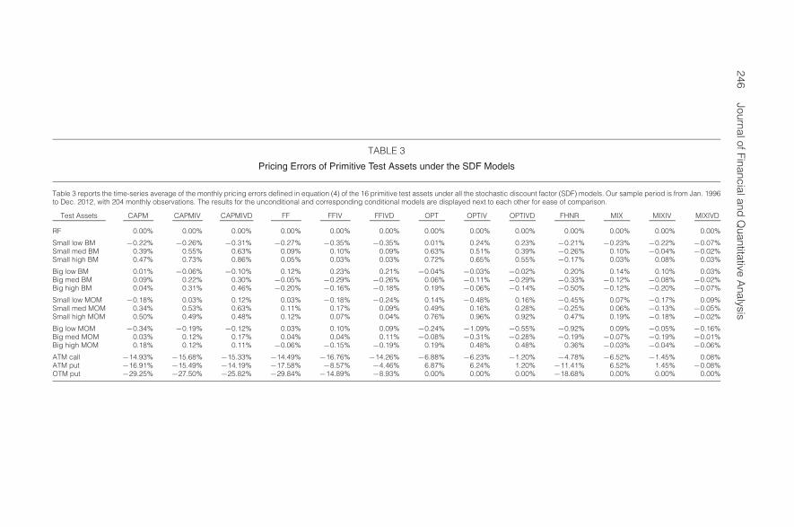
Table 3 reports time-series averages of the monthly pricing errors (alphas), asdefined in equation (4), of the 16 test assets under all the SDF models. The resultsfor the unconditional and corresponding conditional models are displayed next toeach other for ease of comparison. The risk-free rate helps anchor the mean of theSDF models, and as a result, most models can price the risk-free rate well. CAPM,CAPMIV, and CAPMIVD, which do not include the SMB and HML factors, tendto have big pricing errors for the size and book-to-market portfolios. In contrast,by including the SMB and HML factors, FF, FFIV, and FFIVD have much smallerpricing errors for the size and book-to-market portfolios. Most models withoutoption factors have relatively large pricing errors for the ATM calls, ATM puts,and OTM puts. For example, the pricing errors of the three options range fromabout −9% to −30% for CAPM and FF type of models. Although FHNR (2008)includes option straddle factors, it still has relatively large pricing errors for thethree options, with pricing errors ranging from about 5% to 18%. By includingthe STR and SKEW factors, OPT, OPTIV, and OPTIVD reduce the pricing errorsof the three options to about 6% to 7%. Finally, MIX, MIXIV, and MIXIVDhave small pricing errors for both the 12 stock portfolios and the option returns,

However, the exponential models do not perform better than the linear models we considered, and wedo not report them in this article.

246JournalofFinancialand

Quantitative

Analysis

TABLE 3

Pricing Errors of Primitive Test Assets under the SDF Models

Table 3 reports the time-series average of the monthly pricing errors defined in equation (4) of the 16 primitive test assets under all the stochastic discount factor (SDF) models. Our sample period is from Jan. 1996to Dec. 2012, with 204 monthly observations. The results for the unconditional and corresponding conditional models are displayed next to each other for ease of comparison.

Test Assets CAPM CAPMIV CAPMIVD FF FFIV FFIVD OPT OPTIV OPTIVD FHNR MIX MIXIV MIXIVD

RF 0.00% 0.00% 0.00% 0.00% 0.00% 0.00% 0.00% 0.00% 0.00% 0.00% 0.00% 0.00% 0.00%

Small low BM −0.22% −0.26% −0.31% −0.27% −0.35% −0.35% 0.01% 0.24% 0.23% −0.21% −0.23% −0.22% −0.07%Small med BM 0.39% 0.55% 0.63% 0.09% 0.10% 0.09% 0.63% 0.51% 0.39% −0.26% 0.10% −0.04% −0.02%Small high BM 0.47% 0.73% 0.86% 0.05% 0.03% 0.03% 0.72% 0.65% 0.55% −0.17% 0.03% 0.08% 0.03%

Big low BM 0.01% −0.06% −0.10% 0.12% 0.23% 0.21% −0.04% −0.03% −0.02% 0.20% 0.14% 0.10% 0.03%Big med BM 0.09% 0.22% 0.30% −0.05% −0.29% −0.26% 0.06% −0.11% −0.29% −0.33% −0.12% −0.08% −0.02%Big high BM 0.04% 0.31% 0.46% −0.20% −0.16% −0.18% 0.19% −0.06% −0.14% −0.50% −0.12% −0.20% −0.07%

Small low MOM −0.18% 0.03% 0.12% 0.03% −0.18% −0.24% 0.14% −0.48% 0.16% −0.45% 0.07% −0.17% 0.09%Small med MOM 0.34% 0.53% 0.63% 0.11% 0.17% 0.09% 0.49% 0.16% 0.28% −0.25% 0.06% −0.13% −0.05%Small high MOM 0.50% 0.49% 0.48% 0.12% 0.07% 0.04% 0.76% 0.96% 0.92% 0.47% 0.19% −0.18% −0.02%

Big low MOM −0.34% −0.19% −0.12% 0.03% 0.10% 0.09% −0.24% −1.09% −0.55% −0.92% 0.09% −0.05% −0.16%Big med MOM 0.03% 0.12% 0.17% 0.04% 0.04% 0.11% −0.08% −0.31% −0.28% −0.19% −0.07% −0.19% −0.01%Big high MOM 0.18% 0.12% 0.11% −0.06% −0.15% −0.19% 0.19% 0.48% 0.48% 0.36% −0.03% −0.04% −0.06%

ATM call −14.93% −15.68% −15.33% −14.49% −16.76% −14.26% −6.88% −6.23% −1.20% −4.78% −6.52% −1.45% 0.08%ATM put −16.91% −15.49% −14.19% −17.58% −8.57% −4.46% 6.87% 6.24% 1.20% −11.41% 6.52% 1.45% −0.08%OTM put −29.25% −27.50% −25.82% −29.84% −14.89% −8.93% 0.00% 0.00% 0.00% −18.68% 0.00% 0.00% 0.00%


highlighting the importance of including both stock and option factors for pricingthe 16 test assets.18

In summary, the results in Tables 2 and 3 show that certain SDF models(e.g., MIX and most conditional models) can price the 16 primitive test assetsreasonably well. The conditional models can be further improved by using time-averaged factors instead of monthly factors. In fact, these SDF models cannot berejected by the specification test based on the HJ-distance. Because no model isperfect, the key in performance evaluation is to adjust the potential biases of theSDF models in actual applications. The SDF framework of FFJT (2002) providesa common platform on which we can examine this issue and make appropriateadjustments.

B. Evaluating Simulated Hedge Fund Returns

Before applying the above SDF models to evaluate actual hedge fund returns,we first examine their ability to identify abnormal performance in a controlledexperiment where the manager’s ability to deliver superior return is known. Basedon the simulation procedure described in Section II, we generate monthly returnsof a simulated long/short equity fund at different levels of γ, which reflects differ-ent levels of the manager’s ability to forecast future idiosyncratic returns.Following FFJT (2002), we evaluate the performance of the artificial hedge fundby estimating the SDF models using the returns of the fund and the 16 primi-tive assets.

The simulation procedure in Section II does not take fees into account. Giventhat the actual hedge fund returns are net of fee, our simulations consider bothbefore- and after-fee returns by incorporating management and incentive fees, aswell as a standard high-watermark provision.19 The management and incentivefees for most funds are slightly lower than 2% and 20%, respectively. We adoptan aggressive fee structure with a 2% annual management fee and 20% incentivefee to obtain the simulated after-fee returns.20

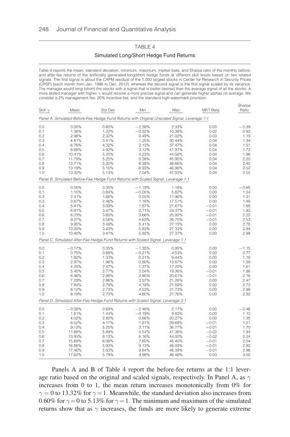
Table 4 provides summary information on simulated hedge fund returns.Specifically, it reports the mean, standard deviation, minimum, maximum, marketbeta, and Sharpe ratio of the monthly returns of the simulated hedge funds at dif-ferent skill levels. We report before- and after-fee returns based on scaled andunscaled signals at different leverage ratios.

18One possible reason for the large option pricing errors could be the fixed weighting matrix used inHJ-distance estimation, which is the inverse of the second moments of the asset returns. The weightingmatrix puts more (less) weight on assets with smaller (higher) second moments, which lead to small(large) pricing errors for assets with small (large) second moments (e.g., the risk-free asset (options)).For future work, it might be interesting to use an identify matrix as the weighting matrix for modelestimation, which might reduce the pricing errors for options.

19We thank the referee for suggesting that we consider after-fee returns.20We do not directly consider transaction costs in our simulation exercise. According to Chordia,

Roll, and Subrahmanyam (2011), the median proportional effective bid–ask spread is about 11 basispoints (bps) (2 bps) between 1993 and 2000 (2000 and 2008). According to Bekaert and Hodrick(2012), the total trading costs (commission, bid–ask spread, and market impact) for larger cap stocksin the United States are about 40 bps in 2005 and 2010. In our simulation exercise, we consideronly the largest 1,000 stocks after 1996, and our simulated portfolios are rebalanced every month.Assuming a 100% monthly turnover, transaction costs, ranging between 2 bps and 40 bps, wouldlower our simulated returns accordingly. But compared to the magnitude of simulated returns, thetransaction cost would have only a minor effect on our later analysis of actual fund performance.


TABLE 4

Simulated Long/Short Hedge Fund Returns

Table 4 reports the mean, standard deviation, minimum, maximum, market beta, and Sharpe ratio of the monthly before-and after-fee returns of the artificially generated long/short hedge funds at different skill levels based on two relatedsignals. The first signal is about the CAPM residual of the 1,000 largest stocks in Center for Research in Security Prices(CRSP) (each month from Jan. 1996 to Dec. 2012), whereas the second signal is the first signal scaled by its variance.The manager would long (short) the stocks with a signal that is better (worse) than the average signal of all the stocks. Amore skilled manager with higher γ would receive a more precise signal and can generate higher alphas on average. Weconsider a 2% management fee, 20% incentive fee, and the standard high-watermark provision.

SharpeSkill γ Mean Std Dev Min Max MKT Beta Ratio

Panel A. Simulated Before-Fee Hedge Fund Returns with Original Unscaled Signal, Leverage 1:1

0.0 0.00% 0.60% −2.38% 2.33% 0.00 −0.390.1 1.36% 1.22% −0.32% 10.38% 0.02 0.930.2 2.98% 2.32% 0.49% 21.02% 0.03 1.190.3 4.81% 3.41% 1.25% 30.44% 0.04 1.340.4 6.76% 4.32% 2.12% 37.47% 0.04 1.510.5 8.68% 4.92% 3.12% 41.97% 0.04 1.720.6 10.41% 5.20% 4.23% 44.56% 0.04 1.960.7 11.79% 5.25% 5.38% 45.95% 0.04 2.200.8 12.71% 5.20% 6.38% 46.66% 0.04 2.400.9 13.19% 5.15% 6.93% 46.96% 0.04 2.521.0 13.32% 5.13% 7.04% 47.03% 0.04 2.55

Panel B. Simulated Before-Fee Hedge Fund Returns with Scaled Signal, Leverage 1:1

0.0 0.00% 0.35% −1.19% 1.18% 0.00 −0.650.1 1.10% 0.84% −0.05% 5.82% 0.00 1.040.2 2.41% 1.66% 0.55% 11.96% 0.00 1.310.3 3.87% 2.46% 1.16% 17.51% 0.00 1.480.4 5.41% 3.09% 1.87% 21.67% −0.01 1.680.5 6.91% 3.47% 2.71% 24.37% −0.01 1.930.6 8.23% 3.60% 3.66% 25.92% −0.01 2.220.7 9.27% 3.58% 4.63% 26.75% −0.01 2.530.8 9.95% 3.49% 5.41% 27.15% 0.00 2.780.9 10.30% 3.43% 5.83% 27.33% 0.00 2.941.0 10.40% 3.41% 5.92% 27.37% 0.00 2.98

Panel C. Simulated After-Fee Hedge Fund Returns with Scaled Signal, Leverage 1:1

0.0 −0.17% 0.35% −1.35% 0.95% 0.00 −1.150.1 0.75% 0.68% −0.21% 4.53% 0.00 0.770.2 1.80% 1.33% 0.31% 9.44% 0.00 1.180.3 2.97% 1.96% 0.80% 13.87% 0.00 1.390.4 4.20% 2.47% 1.37% 17.20% 0.00 1.610.5 5.40% 2.77% 2.04% 19.36% −0.01 1.860.6 6.46% 2.88% 2.80% 20.61% −0.01 2.160.7 7.29% 2.86% 3.57% 21.26% 0.00 2.470.8 7.84% 2.79% 4.19% 21.59% 0.00 2.720.9 8.12% 2.74% 4.53% 21.73% 0.00 2.881.0 8.19% 2.73% 4.60% 21.76% 0.00 2.92

Panel D. Simulated After-Fee Hedge Fund Returns with Scaled Signal, Leverage 2:1

0.0 −0.09% 0.69% −2.46% 2.17% 0.00 −0.460.1 1.81% 1.44% −0.19% 9.83% 0.00 1.100.2 4.02% 2.82% 0.86% 20.27% 0.00 1.350.3 6.52% 4.17% 1.91% 29.69% −0.01 1.510.4 9.13% 5.25% 3.11% 36.77% −0.01 1.700.5 11.68% 5.89% 4.54% 41.36% −0.02 1.940.6 13.93% 6.13% 6.16% 44.00% −0.02 2.240.7 15.69% 6.08% 7.80% 45.40% −0.01 2.540.8 16.86% 5.93% 9.13% 46.09% −0.01 2.800.9 17.46% 5.83% 9.84% 46.39% −0.01 2.961.0 17.62% 5.79% 9.99% 46.46% 0.00 3.00

Panels A and B of Table 4 report the before-fee returns at the 1:1 lever-age ratio based on the original and scaled signals, respectively. In Panel A, as γincreases from 0 to 1, the mean return increases monotonically from 0% forγ = 0 to 13.32% for γ=1. Meanwhile, the standard deviation also increases from0.60% for γ=0 to 5.13% for γ=1. The minimum and maximum of the simulatedreturns show that as γ increases, the funds are more likely to generate extreme


positive returns. The betas of the artificial hedge fund returns are not exactly 0but are generally low. The returns in Panel B based on the scaled signal havelower mean, lower standard deviation, and less dispersion, but higher Sharperatio than those in Panel A, because less money would be put into stocks withmore volatile idiosyncratic risk. The higher Sharpe ratio is consistent with theidea that the scaled signal reflects a better trade-off between risk and return thanthe unscaled signal. The betas of the simulated returns based on the scaled signalare also closer to 0.

The after-fee returns based on the scaled signal at the 1:1 leverage ratioreported in Panel C of Table 4 are obviously lower than the before-fee returns andmore significantly so for higher manager skill levels. For instance, for γ=0.2, theaverage monthly after-fee return is 1.80%, which is 61 bps lower than the averagebefore-fee return in Panel B. For γ = 0.9, however, the average monthly after-fee return based on the scaled signal becomes 8.12%, which is 2.28% less thanthe before-fee return in Panel B. This indicates that when the manager skill levelincreases, managers deliver more abnormal returns and at the same time earnmore fees.

Panel D of Table 4 reports the after-fee returns based on the scaled signalwith a 2:1 leverage ratio. Intuitively, when the leverage ratio is high, managers aremore willing to take risk and the fund returns are higher, with higher volatilities.For the higher leverage ratio of 2:1, when γ increase from 0.1 to 0.9, the averagefund returns increase from 1.81% to 17.46%; for the lower leverage ratio of 1:1,the corresponding numbers are 0.75% and 8.12%.

Our ultimate goal is to use the simulated returns as a benchmark to evaluateactual hedge fund returns. Therefore, for the rest of the article, we mainly focus onafter-fee returns based on the scaled signal at different leverage ratios to better re-flect the reality of how hedge fund managers make investment decisions and howinvestors evaluate hedge funds. A natural question is whether the simulated re-turns resemble the actual hedge fund returns. As discussed in Section II, the setupof the simulation mimics stock-picking practices in reality. Comparing Panel C ofTable 1 with Table 4, we see that the magnitudes of the simulated hedge fund re-turns are reasonably close to those of the actual hedge fund returns. In results notreported here, we also show that when the skill level γ is lower than 0.2, the simu-lated hedge fund returns exhibit nonlinear exposures to risk factors that are similarto those documented in Panel D of Table 1 for the actual hedge fund returns.

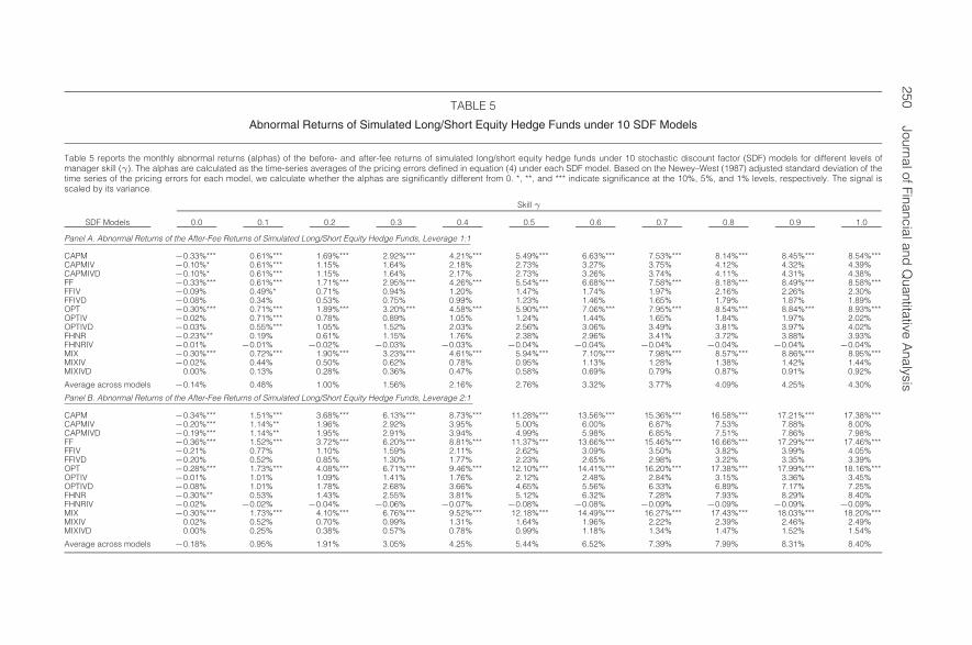
Next, we apply the SDF models to evaluate the simulated hedge fund returnsbased on the scaled signal. Panels A and B of Table 5 report the alphas of themonthly after-fee returns under each SDF model for leverage ratios of 1:1 and 2:1,respectively. The alphas are calculated as the time-series average of the pricing er-rors defined in equation (4) under each SDF model. Based on the Newey–West(1987) adjusted standard deviation of the time series of the pricing errors, we ex-amine whether the pricing errors are significantly different from 0 at the 10% (*),5% (**), and 1% (***) levels. In Panel A, when γ = 0 (i.e., the manager has nosuperior ability to forecast future returns), the alphas for the after-fee returns un-der most models are negative, between −0.33% and 0. This finding is consistentwith that of FFJT (2002), where the alphas under most models exhibit a slightnegative bias when mutual fund managers do not have any ability to outperform

250JournalofFinancialand

Quantitative

Analysis

TABLE 5

Abnormal Returns of Simulated Long/Short Equity Hedge Funds under 10 SDF Models

Table 5 reports the monthly abnormal returns (alphas) of the before- and after-fee returns of simulated long/short equity hedge funds under 10 stochastic discount factor (SDF) models for different levels ofmanager skill (γ). The alphas are calculated as the time-series averages of the pricing errors defined in equation (4) under each SDF model. Based on the Newey–West (1987) adjusted standard deviation of thetime series of the pricing errors for each model, we calculate whether the alphas are significantly different from 0. *, **, and *** indicate significance at the 10%, 5%, and 1% levels, respectively. The signal isscaled by its variance.

Skill γ

SDF Models 0.0 0.1 0.2 0.3 0.4 0.5 0.6 0.7 0.8 0.9 1.0

Panel A. Abnormal Returns of the After-Fee Returns of Simulated Long/Short Equity Hedge Funds, Leverage 1:1

CAPM −0.33%*** 0.61%*** 1.69%*** 2.92%*** 4.21%*** 5.49%*** 6.63%*** 7.53%*** 8.14%*** 8.45%*** 8.54%***CAPMIV −0.10%* 0.61%*** 1.15% 1.64% 2.18% 2.73% 3.27% 3.75% 4.12% 4.32% 4.39%CAPMIVD −0.10%* 0.61%*** 1.15% 1.64% 2.17% 2.73% 3.26% 3.74% 4.11% 4.31% 4.38%FF −0.33%*** 0.61%*** 1.71%*** 2.95%*** 4.26%*** 5.54%*** 6.68%*** 7.58%*** 8.18%*** 8.49%*** 8.58%***FFIV −0.09% 0.49%* 0.71% 0.94% 1.20% 1.47% 1.74% 1.97% 2.16% 2.26% 2.30%FFIVD −0.08% 0.34% 0.53% 0.75% 0.99% 1.23% 1.46% 1.65% 1.79% 1.87% 1.89%OPT −0.30%*** 0.71%*** 1.89%*** 3.20%*** 4.58%*** 5.90%*** 7.06%*** 7.95%*** 8.54%*** 8.84%*** 8.93%***OPTIV −0.02% 0.71%*** 0.78% 0.89% 1.05% 1.24% 1.44% 1.65% 1.84% 1.97% 2.02%OPTIVD −0.03% 0.55%*** 1.05% 1.52% 2.03% 2.56% 3.06% 3.49% 3.81% 3.97% 4.02%FHNR −0.23%** 0.19% 0.61% 1.15% 1.76% 2.38% 2.96% 3.41% 3.72% 3.88% 3.93%FHNRIV −0.01% −0.01% −0.02% −0.03% −0.03% −0.04% −0.04% −0.04% −0.04% −0.04% −0.04%MIX −0.30%*** 0.72%*** 1.90%*** 3.23%*** 4.61%*** 5.94%*** 7.10%*** 7.98%*** 8.57%*** 8.86%*** 8.95%***MIXIV −0.02% 0.44% 0.50% 0.62% 0.78% 0.95% 1.13% 1.28% 1.38% 1.42% 1.44%MIXIVD 0.00% 0.13% 0.28% 0.36% 0.47% 0.58% 0.69% 0.79% 0.87% 0.91% 0.92%

Average across models −0.14% 0.48% 1.00% 1.56% 2.16% 2.76% 3.32% 3.77% 4.09% 4.25% 4.30%

Panel B. Abnormal Returns of the After-Fee Returns of Simulated Long/Short Equity Hedge Funds, Leverage 2:1

CAPM −0.34%*** 1.51%*** 3.68%*** 6.13%*** 8.73%*** 11.28%*** 13.56%*** 15.36%*** 16.58%*** 17.21%*** 17.38%***CAPMIV −0.20%*** 1.14%** 1.96% 2.92% 3.95% 5.00% 6.00% 6.87% 7.53% 7.88% 8.00%CAPMIVD −0.19%*** 1.14%** 1.95% 2.91% 3.94% 4.99% 5.98% 6.85% 7.51% 7.86% 7.98%FF −0.36%*** 1.52%*** 3.72%*** 6.20%*** 8.81%*** 11.37%*** 13.66%*** 15.46%*** 16.66%*** 17.29%*** 17.46%***FFIV −0.21% 0.77% 1.10% 1.59% 2.11% 2.62% 3.09% 3.50% 3.82% 3.99% 4.05%FFIVD −0.20% 0.52% 0.85% 1.30% 1.77% 2.23% 2.65% 2.98% 3.22% 3.35% 3.39%OPT −0.28%*** 1.73%*** 4.08%*** 6.71%*** 9.46%*** 12.10%*** 14.41%*** 16.20%*** 17.38%*** 17.99%*** 18.16%***OPTIV −0.01% 1.01% 1.09% 1.41% 1.76% 2.12% 2.48% 2.84% 3.15% 3.36% 3.45%OPTIVD −0.08% 1.01% 1.78% 2.68% 3.66% 4.65% 5.56% 6.33% 6.89% 7.17% 7.25%FHNR −0.30%** 0.53% 1.43% 2.55% 3.81% 5.12% 6.32% 7.28% 7.93% 8.29% 8.40%FHNRIV −0.02% −0.02% −0.04% −0.06% −0.07% −0.08% −0.08% −0.09% −0.09% −0.09% −0.09%MIX −0.30%*** 1.73%*** 4.10%*** 6.76%*** 9.52%*** 12.18%*** 14.49%*** 16.27%*** 17.43%*** 18.03%*** 18.20%***MIXIV 0.02% 0.52% 0.70% 0.99% 1.31% 1.64% 1.96% 2.22% 2.39% 2.46% 2.49%MIXIVD 0.00% 0.25% 0.38% 0.57% 0.78% 0.99% 1.18% 1.34% 1.47% 1.52% 1.54%

Average across models −0.18% 0.95% 1.91% 3.05% 4.25% 5.44% 6.52% 7.39% 7.99% 8.31% 8.40%


the market. When γ ≥ 0.1, we find positive alphas that increase with γ undermost SDF models. Interestingly, most models lead to similar inferences regard-ing the abnormal performance of the simulated hedge funds. The alphas undermost of the unconditional models share similar magnitudes for a given γ. For in-stance, when γ increases from 0.1 to 0.9, the after-fee monthly alphas for mostunconditional models increase from less than 1% to around 8.5%. The conditionalmodels with either monthly information or time-averaged factors have a similarpattern, but on average have smaller alphas than the unconditional models, espe-cially for SDFs with time-averaged factors. When γ increases from 0.1 to 0.9, theafter-fee monthly alphas for the conditional models increase from less than 1% toaround 2% to 4%. This suggests that part of the alphas under the unconditionalmodels may be attributable to time-varying market prices of risks or interim trad-ing. There is a concern that the conditional models might have too many factors,which tend to overfit the data and lead to smaller but more volatile pricing errors.For instance, though most alphas are small and not statistically significant underFHNRIV, the model could have overfitted the data and failed to detect true skills.Based on results presented in Panel B, we reach similar conclusions about theperformance of hedge funds with a 2:1 leverage ratio, though this higher leverageratio leads to higher alphas.

Overall, the results in Tables 4 and 5 show that most of the SDF models de-liver similar evaluation results: They are able to detect the abnormal performanceof the simulated hedge fund returns, though most models exhibit a slight negativebias when the managers have no skill. Therefore, at least in situations that arenot too different from our simulation setup, the SDF approach of FFJT (2002) isan effective methodology for evaluating hedge fund performance (after correctingfor the negative bias).

C. Evaluating Actual Hedge Fund Performance

In this section, we apply the SDF models to evaluate the performances of2,315 long/short equity hedge funds. Following FFJT (2002), we evaluate theperformance of an actual hedge fund by estimating the SDF models using thereturns of the hedge fund and the 16 primitive test assets.

TASS directly reports after-fee hedge fund returns. However, there is a con-cern that because of illiquid assets held by some hedge funds, stale prices maycause the observed raw returns of the hedge funds to be biased. To correct forthe potential bias caused by stale prices in hedge fund returns, Getmansky et al.(2004) fit econometric models (e.g., autoregressive moving average (ARMA)models) to hedge fund returns to remove autocorrelations induced by stale prices.The residuals plus the intercepts from the fitted model are then used as “actual”hedge fund returns for performance evaluation. In our situation, long/short equityfunds are more likely to use equity and equity derivatives, which are relativelyeasy to trade. As a result, the bias for long/short equity funds might be less severethan that for funds that hold illiquid assets (e.g., real estate). Still, to be conserva-tive, following Getmansky et al., we fit an ARMA(1, 1) model to the actual hedgefund returns and then use the residuals as “actual” hedge fund returns to rank theirperformance.


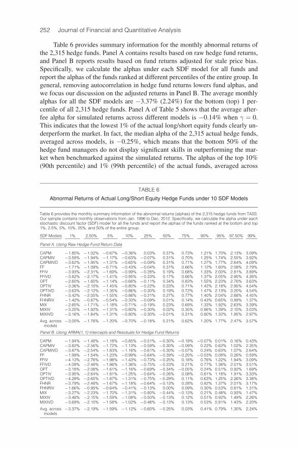
Table 6 provides summary information for the monthly abnormal returns ofthe 2,315 hedge funds. Panel A contains results based on raw hedge fund returns,and Panel B reports results based on fund returns adjusted for stale price bias.Specifically, we calculate the alphas under each SDF model for all funds andreport the alphas of the funds ranked at different percentiles of the entire group. Ingeneral, removing autocorrelation in hedge fund returns lowers fund alphas, andwe focus our discussion on the adjusted returns in Panel B. The average monthlyalphas for all the SDF models are −3.37% (2.24%) for the bottom (top) 1 per-centile of all 2,315 hedge funds. Panel A of Table 5 shows that the average after-fee alpha for simulated returns across different models is −0.14% when γ = 0.This indicates that the lowest 1% of the actual long/short equity funds clearly un-derperform the market. In fact, the median alpha of the 2,315 actual hedge funds,averaged across models, is −0.25%, which means that the bottom 50% of thehedge fund managers do not display significant skills in outperforming the mar-ket when benchmarked against the simulated returns. The alphas of the top 10%(90th percentile) and 1% (99th percentile) of the actual funds, averaged across

TABLE 6

Abnormal Returns of Actual Long/Short Equity Hedge Funds under 10 SDF Models

Table 6 provides the monthly summary information of the abnormal returns (alphas) of the 2,315 hedge funds from TASS.Our sample contains monthly observations from Jan. 1996 to Dec. 2012. Specifically, we calculate the alpha under eachstochastic discount factor (SDF) model for all the funds and report the alphas of the funds ranked at the bottom and top1%, 2.5%, 5%, 10%, 25%, and 50% of the entire group.

SDF Models 1% 2.50% 5% 10% 25% 50% 75% 90% 95% 97.50% 99%

Panel A. Using Raw Hedge Fund Return Data

CAPM −1.85% −1.02% −0.67% −0.36% 0.03% 0.37% 0.73% 1.21% 1.70% 2.13% 3.09%CAPMIV −3.58% −1.94% −1.17% −0.63% −0.07% 0.31% 0.70% 1.25% 1.74% 2.55% 3.92%CAPMIVD −3.62% −1.95% −1.31% −0.65% −0.09% 0.31% 0.71% 1.27% 1.77% 2.64% 4.09%FF −1.71% −1.09% −0.71% −0.43% −0.04% 0.31% 0.66% 1.12% 1.60% 2.08% 2.79%FFIV −3.93% −2.31% −1.69% −0.99% −0.28% 0.19% 0.68% 1.33% 2.00% 2.81% 3.89%FFIVD −3.82% −2.17% −1.41% −0.95% −0.33% 0.17% 0.66% 1.37% 2.05% 2.90% 4.26%OPT −2.60% −1.60% −1.14% −0.66% −0.11% 0.34% 0.83% 1.55% 2.23% 2.76% 3.63%OPTIV −3.36% −2.10% −1.45% −0.80% −0.22% 0.23% 0.71% 1.42% 2.18% 2.95% 4.54%OPTIVD −3.63% −2.12% −1.35% −0.86% −0.30% 0.19% 0.72% 1.47% 2.13% 3.20% 4.54%FHNR −3.42% −2.05% −1.55% −0.86% −0.21% 0.27% 0.77% 1.40% 2.04% 2.88% 4.45%FHNRIV −1.42% −0.87% −0.54% −0.33% −0.09% 0.01% 0.14% 0.43% 0.65% 0.99% 1.37%MIX −2.65% −1.71% −1.18% −0.71% −0.19% 0.23% 0.69% 1.33% 1.92% 2.63% 3.39%MIXIV −3.20% −1.92% −1.31% −0.80% −0.30% 0.02% 0.35% 0.86% 1.39% 2.10% 3.03%MIXIVD −3.16% −1.84% −1.31% −0.80% −0.30% −0.01% 0.31% 0.80% 1.32% 1.95% 2.97%

Avg. across −3.00% −1.76% −1.20% −0.70% −0.18% 0.21% 0.62% 1.20% 1.77% 2.47% 3.57%models

Panel B. Using ARMA(1, 1) Intercepts and Residuals for Hedge Fund Returns

CAPM −1.94% −1.48% −1.18% −0.85% −0.51% −0.30% −0.19% −0.07% 0.01% 0.16% 0.43%CAPMIV −3.82% −2.56% −1.72% −1.13% −0.59% −0.30% −0.09% 0.22% 0.62% 1.02% 2.35%CAPMIVD −3.87% −2.54% −1.83% −1.16% −0.61% −0.30% −0.07% 0.24% 0.63% 1.07% 2.64%FF −1.99% −1.54% −1.23% −0.99% −0.64% −0.39% −0.20% −0.03% 0.08% 0.26% 0.59%FFIV −4.13% −2.76% −1.98% −1.43% −0.73% −0.25% 0.18% 0.76% 1.22% 1.94% 3.09%FFIVD −4.09% −2.48% −1.86% −1.36% −0.75% −0.23% 0.21% 0.77% 1.38% 2.01% 3.51%OPT −3.18% −2.08% −1.61% −1.16% −0.69% −0.34% −0.05% 0.24% 0.51% 0.92% 1.69%OPTIV −3.95% −2.64% −1.81% −1.25% −0.64% −0.26% 0.08% 0.61% 1.18% 1.91% 3.33%OPTIVD −4.29% −2.65% −1.87% −1.31% −0.75% −0.29% 0.11% 0.63% 1.25% 2.26% 3.38%FHNR −3.79% −2.48% −1.67% −1.18% −0.64% −0.13% 0.28% 0.82% 1.37% 2.01% 3.17%FHNRIV −1.66% −0.95% −0.64% −0.41% −0.13% 0.00% 0.09% 0.30% 0.53% 0.81% 1.31%MIX −3.27% −2.23% −1.70% −1.31% −0.80% −0.44% −0.13% 0.21% 0.48% 0.93% 1.47%MIXIV −3.48% −2.15% −1.59% −1.08% −0.50% −0.13% 0.12% 0.51% 0.92% 1.49% 2.26%MIXIVD −3.69% −2.10% −1.58% −1.02% −0.48% −0.13% 0.13% 0.53% 0.91% 1.43% 2.20%

Avg. across −3.37% −2.19% −1.59% −1.12% −0.60% −0.25% 0.03% 0.41% 0.79% 1.30% 2.24%models


models, roughly correspond to the alphas of the simulated funds with γ ∈ (0, 0.1)and γ ∈ (0.4, 0.5), respectively. Overall, these results show that the bottom halfof the actual hedge funds cannot deliver abnormal performance, whereas the verytop fund managers clearly have substantial skills.

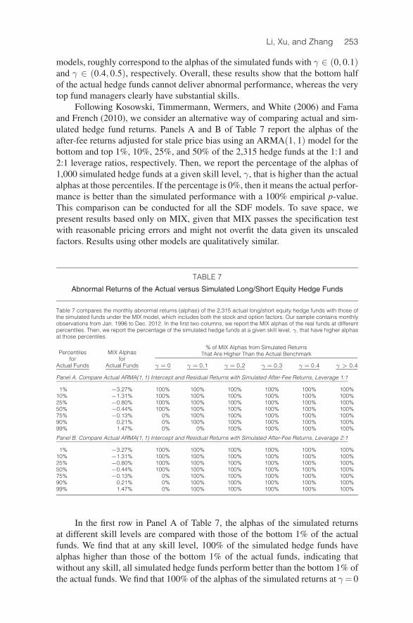
Following Kosowski, Timmermann, Wermers, and White (2006) and Famaand French (2010), we consider an alternative way of comparing actual and sim-ulated hedge fund returns. Panels A and B of Table 7 report the alphas of theafter-fee returns adjusted for stale price bias using an ARMA(1, 1) model for thebottom and top 1%, 10%, 25%, and 50% of the 2,315 hedge funds at the 1:1 and2:1 leverage ratios, respectively. Then, we report the percentage of the alphas of1,000 simulated hedge funds at a given skill level, γ, that is higher than the actualalphas at those percentiles. If the percentage is 0%, then it means the actual perfor-mance is better than the simulated performance with a 100% empirical p-value.This comparison can be conducted for all the SDF models. To save space, wepresent results based only on MIX, given that MIX passes the specification testwith reasonable pricing errors and might not overfit the data given its unscaledfactors. Results using other models are qualitatively similar.

TABLE 7

Abnormal Returns of the Actual versus Simulated Long/Short Equity Hedge Funds

Table 7 compares the monthly abnormal returns (alphas) of the 2,315 actual long/short equity hedge funds with those ofthe simulated funds under the MIX model, which includes both the stock and option factors. Our sample contains monthlyobservations from Jan. 1996 to Dec. 2012. In the first two columns, we report the MIX alphas of the real funds at differentpercentiles. Then, we report the percentage of the simulated hedge funds at a given skill level, γ, that have higher alphasat those percentiles.

% of MIX Alphas from Simulated ReturnsThat Are Higher Than the Actual BenchmarkPercentiles MIX Alphas

for forActual Funds Actual Funds γ = 0 γ = 0.1 γ = 0.2 γ = 0.3 γ = 0.4 γ > 0.4

Panel A. Compare Actual ARMA(1, 1) Intercept and Residual Returns with Simulated After-Fee Returns, Leverage 1:1

1% −3.27% 100% 100% 100% 100% 100% 100%10% −1.31% 100% 100% 100% 100% 100% 100%25% −0.80% 100% 100% 100% 100% 100% 100%50% −0.44% 100% 100% 100% 100% 100% 100%75% −0.13% 0% 100% 100% 100% 100% 100%90% 0.21% 0% 100% 100% 100% 100% 100%99% 1.47% 0% 0% 100% 100% 100% 100%

Panel B. Compare Actual ARMA(1, 1) Intercept and Residual Returns with Simulated After-Fee Returns, Leverage 2:1

1% −3.27% 100% 100% 100% 100% 100% 100%10% −1.31% 100% 100% 100% 100% 100% 100%25% −0.80% 100% 100% 100% 100% 100% 100%50% −0.44% 100% 100% 100% 100% 100% 100%75% −0.13% 0% 100% 100% 100% 100% 100%90% 0.21% 0% 100% 100% 100% 100% 100%99% 1.47% 0% 100% 100% 100% 100% 100%

In the first row in Panel A of Table 7, the alphas of the simulated returnsat different skill levels are compared with those of the bottom 1% of the actualfunds. We find that at any skill level, 100% of the simulated hedge funds havealphas higher than those of the bottom 1% of the actual funds, indicating thatwithout any skill, all simulated hedge funds perform better than the bottom 1% ofthe actual funds. We find that 100% of the alphas of the simulated returns at γ=0


are higher than those of the bottom 50% of the actual funds, again suggesting thatthe bottom 50% of the actual funds do not seem to possess any ability to out-perform the market. The top 25% of the actual hedge funds have alphas that aresignificantly higher than the simulated alphas with γ = 0 but not with γ ≥ 0.1.The top 10% (1%) of the actual funds have alphas higher than the simulatedreturns with γ < 0.1 (γ < 0.2). When the leverage ratio is increased to 2:1 inPanel B, the top 50% of the actual funds have alphas higher than the simulatedalphas with γ = 0 but not with γ ≥ 0.1. Remember that when γ is around 0.1 to0.2, if we regress the signals, sit, on the realized residue εit, the R2 is merely 1%to 4%. Results in Panel B of Table 7 clearly show that most funds do not have theability to outperform the market.

We need to keep in mind a few caveats about the above analysis. Obviously,our simulation is based on several stylized assumptions. First, we assume 0 trans-action costs, which makes high turnover costless. This assumption tends to inflatethe performance of simulated returns. Meanwhile, there is a possibility that thesimulated returns can be biased downward, because we assume an aggressivefee structure as well as low leverage ratio. Finally, we assume that most of thelong/short equity funds follow a strategy similar to that used in our simulation.But in reality, the long/short equity style is the most diverse hedge fund style, andthe managers could implement a wide range of different strategies (note that themaximum return for the top 25% of hedge funds in Panel C of Table 1 is manytimes greater than that of the simulated hedge funds). The key to any simulation isthat it needs to mimic the returns of hedge funds to be evaluated. Although we cannever be sure that our simulation mimics every long/short equity fund in reality,we believe the basic approach illustrated here is useful.

Overall, given our assumptions, our results show that although most hedgefunds cannot beat the market, there is a small percentage of hedge funds thatdo seem to be able to outperform the market. Most important, our analysis showsthat the general approach of FFJT (2002) is applicable to hedge fund performanceevaluation.

VI. Conclusion

Hedge fund performance evaluation is a timely and challenging topic.Finance researchers have only begun to study all the intricacies of hedgefund returns. Our article contributes to this growing literature by showing thatthe SDF approach of FFJT (2002), which was to evaluate mutual fund perfor-mance, is equally applicable to hedge funds. To accommodate hedge funds’ usageof dynamic trading strategies and derivatives, we extend the FFJT approach byconsidering models with option and time-averaged factors and incorporatingoption returns in model estimation. By simulating returns of hedge funds whosemanagers have known ability to outperform the market, we study the extent towhich a wide range of SDF models can detect such ability. We show that mostmodels lead to similar conclusions on hedge fund performance. Finally, we applyour approach to evaluate the performance of 2,315 long/short equity hedge fundsand find that the average hedge fund cannot outperform the market, though a smallportion of these hedge funds can.


Appendix. Scaled Signals

We define the signal as

sit = γεit + (1 − γ)σiuit.(A-1)

We can compute the following (for later discussion, we drop all subscripts, i, t, for brevity):

E(s) = E[γε + (1 − γ)σu] = 0,(A-2)

var(s) = var[γε + (1 − γ)σu] = [γ2 + (1 − γ)2]σ2.(A-3)

If we assume u and s are conditional normal, then we have

E(u|s) = E(u) +cov(u, s)

var(s)[s − E(s)](A-4)

=(1 − γ)s

[γ2 + (1 − γ)2]σ,

var(u|s) = var(u)− cov2(u, s)var(s)

(A-5)

= 1 − (1 − γ)2

[γ2 + (1 − γ)2]=

γ2

[γ2 + (1 − γ)2].

Also from equation (A-1), the information ε can be computed as

ε =1γ[s − (1 − γ)σu].(A-6)

Now we can compute the conditional expectation of ε,

E(ε|s) =1γ[s − (1 − γ)σE(u|s)](A-7)

=1γ[s − (1 − γ)σ

(1 − γ)s[γ2 + (1 − γ)2]σ]

=γs

[γ2 + (1 − γ)2],

and the conditional variance of ε,

var(ε|s) = var{1/γ[s − (1 − γ)σu]|s}(A-8)

=(1 − γ)2σ2

γ2var(u|s)

=(1 − γ)2σ2

γ2

γ2

[γ2 + (1 − γ)2]

=(1 − γ)2σ2

[γ2 + (1 − γ)2].

Combining equations (A-7) and (A-8), we have

E(εit|sit)

var(εit|sit)=

γsit

[γ2 + (1 − γ)2]

(1 − γ)2σ2i

[γ2 + (1 − γ)2]

=γ

(1 − γ)2

sit

σ2i

.(A-9)

Notice that for a given manager, the skill level, γ, is a constant. The function is well definedfor any skill level between 0 and 1, including 0. When γ = 1, what the manager observesis the true signal without any noise, and the comparable measure should be εit/σ

2i .


ReferencesAgarwal, V., and N. Y. Naik. “Risks and Portfolio Decisions Involving Hedge Funds.” Review of

Financial Studies, 17 (2004), 63–98.Ahn, S. C., and C. Gadarowski. “Small Sample Properties of the GMM Specification Test Based on

the Hansen–Jagannathan Distance.” Journal of Empirical Finance, 11 (2004), 109–132.Ang, A.; R. J. Hodrick; Y. Xing; and X. Zhang. “The Cross Section of Volatility and Expected

Returns.” Journal of Finance, 61 (2006), 259–299.Bekaert, G., and R. Hodrick, International Financial Management, 2nd ed. Essex, UK: Pearson Edu-

cation (2012).Ben Dor, A.; R. Jagannathan; and I. Meier. “Understanding Mutual Funds and Hedge Funds Styles

Using Return-Based Analysis.” Journal of Investment Management, 1 (2003), 97–137.Cao, C.; Y. Chen; B. Liang; and A. Lo. “Can Hedge Funds Time Market Liquidity?” Journal of

Financial Economics, 109 (2013), 493–516.Chen, Y.; W. Ferson; and H. Peters. “Measuring the Timing Ability and Performance of Bond Mutual

Funds.” Journal of Financial Economics, 98 (2010), 72–89.Chordia, T.; R. Roll; and A. Subrahmanyam. “Recent Trends in Trading Activity and Market Quality.”

Journal of Financial Economics, 101 (2011), 243–263.Cochrane, J. Asset Pricing. Princeton, NJ: Princeton University Press (2005).Dybvig, P. H., and S. A. Ross. “Differential Information and Performance Measurement Using a

Security Market Line.” Journal of Finance, 40 (1985), 383–399.Fama, E., and K. French. “Common Risk Factors in the Returns on Stocks and Bonds.” Journal of

Financial Economics, 33 (1993), 3–56.Fama, E., and K. French. “Luck versus Skill in the Cross-Section of Mutual Fund Returns.” Journal

of Finance, 65 (2010), 1915–1947.Farnsworth, H.; W. Ferson; D. Jackson; and S. Todd. “Performance Evaluation with Stochastic

Discount Factors.” Journal of Business, 75 (2002), 473–583.Ferson, W., and S. R. Foerster. “Finite Sample Properties of the Generalized Methods of Moments

Tests of Conditional Asset Pricing Models.” Journal of Financial Economics, 36 (1994), 29–56.Ferson, W.; T. Henry; and D. Kisgen. “Evaluating Government Bond Fund Performance with Stochas-

tic Discount Factors.” Review of Financial Studies, 19 (2006), 423–455.Ferson, W.; S. Sarkissian; and T. Simin. “Asset Pricing Models with Conditional Alphas and Betas:

The Effects of Data Snooping and Spurious Regression.” Journal of Financial and QuantitativeAnalysis, 43 (2008), 331–354.

Fung, W., and D. A. Hsieh. “Empirical Characteristics of Dynamic Trading Strategies: The Case ofHedge Funds.” Review of Financial Studies, 10 (1997), 275–302.

Fung, W., and D. A. Hsieh. “The Risk in Hedge Fund Strategies: Theory and Evidence from TrendFollowers.” Review of Financial Studies, 14 (2001), 313–341.

Fung, W.; D. A. Hsieh; N. Y. Naik; and T. Ramadorai. “Hedge Funds: Performance, Risk, and CapitalFormation.” Journal of Finance, 63 (2008), 1777–1803.

Getmansky, M.; A. Lo; and I. Makarov. “An Econometric Analysis of Serial Correlation and Illiquidityin Hedge-Fund Returns.” Journal of Financial Economics, 74 (2004), 529–609.

Grinblatt, M., and S. Titman. “Portfolio Performance Evaluation: Old Issues and New Insights.”Review of Financial Studies, 2 (1989), 393–421.

Hansen, L. P., and R. Jagannathan. “Assessing Specification Errors in Stochastic Discount FactorModels.” Journal of Finance, 52 (1997), 557–590.

Jegadeesh, N., and S. Titman. “Returns to Buying Winners and Selling Losers: Implications for StockMarket Efficiency.” Journal of Finance, 48 (1993), 65–91.

Khandani, A., and A. Lo. “What Happened to the Quants in August 2007? Evidence from Factors andTransactions Data.” Journal of Financial Markets, 14 (2011), 1–46.

Kirby, C. “Measuring the Predictable Variation in Stock and Bond Returns.” Review of FinancialStudies, 10 (1997), 579–630.

Kosowski, R.; A. Timmermann; R. Wermers; and H. White. “Can Mutual Fund ‘Stars’ Really PickStocks? New Evidence from a Bootstrap Analysis.” Journal of Finance, 61 (2006), 2551–2595.

Li, H.; Y. Xu; and X. Zhang. “Evaluating Asset Pricing Models Using the Second Hansen-JagannathanDistance.” Journal of Financial Economics, 62 (2010), 327–376.

Merton, R. C. “On Market Timing and Investment Performance: An Equilibrium Theory of Values forMarket Forecasts.” Journal of Business, 54 (1981), 363–406.

Mitchell, M., and T. Pulvino. “Characteristics of Risk and Return in Risk Arbitrage.” Journal ofFinance, 56 (2001), 2135–2175.

Newey, W. K., and K. D. West. “A Simple, Positive Semi-Definite, Heteroskedasticity and Autocorre-lation Consistent Covariance Matrix.” Econometrica, 55 (1987), 703–708.


Patton, A., and T. Ramadorai. “On the High-Frequency Dynamics of Hedge Fund Risk Exposures.”Journal of Finance, 68 (2013), 597–635.

Sharpe, W. F. “Capital Asset Prices: A Theory of Market Equilibrium under Conditions of Risk.”Journal of Finance, 19 (1964), 425–442.

Treynor, J. L., and K. Mazuy. “Can Mutual Funds Outguess the Market?” Harvard Business Review,44 (1966), 131–136.

Hedge Fund Performance Evaluation under the Stochastic ...zhang654/jfqa2016.pdf · and effective...

Documents

Transcript of Hedge Fund Performance Evaluation under the Stochastic ...zhang654/jfqa2016.pdf · and effective...