Hedge fund leverage and performance: New evidence from multiple leveraged share classes1

Pekka Tolonen

Abstract

This study examines hedge funds’ ability to enhance their performance through

leverage. Using a hand-collected sample of fund leverage classes gathered from major

commercial databases, we find that the use of leverage enhances risk-adjusted returns

and risk. The average high-leverage share class underperforms its low-leverage

counterpart for the same investment program after their returns are appropriately

adjusted to the same level. The portfolio being long low-leverage share classes and

short high-leverage share classes constructed to be market neutral, provides positive

and significant risk-adjusted performance during the 1994 – 2012 time period. This

finding is consistent with the theoretical predictions of Frazzini & Pedersen (2013)

and Black (1972) and indicates that leverage constraints and costs of leverage have a

negative impact on risk-adjusted returns.

1 We thank Robert Kosowski and Juha Joenväärä for helpful comments. We thank Mikko Kauppila for help with the data. We are grateful for the support of OP-Pohjola Group Research Foundation. Contact address: Pekka Tolonen, University of Oulu, pekka.tolonen@oulu.fi.

2

1 Introduction

This study examines hedge funds’ ability to enhance their performance through

leverage. Hedge fund management companies often have multiple share classes of the

same investment program, which only differ in their leverage levels. Using a hand-

collected data for levered share classes constructed from the union of major

commercial databases, we show that management companies establish high-leverage

classes of their investment programs that exhibit higher levels of total returns and

volatility. We show that the average high-leverage class of the investment program

underperforms its low-leverage counterpart after the returns (and the risk) of both

classes are adjusted to the same level. Our findings are in line with the theory of

leverage aversion (Frazzini & Pedersen 2013, Asness et al. 2012, Black 1972) and

suggest that costs of leverage and leverage constraints of investors have a negative

impact on returns. The high-leverage classes generate economically and statistically

significant alpha but not to the extent that could be expected based on their level of

leverage.

Leverage is one of the important drivers of returns in hedge fund industry, which

currently manages over $2 trillion of assets. Hedge funds use leverage to exploit

investment opportunities and attain a level of volatility desired by investors. Hedge

funds obtain leverage through direct financing, margin borrowing (e.g., shorting),

derivative transactions (options, futures, etc.), structured products, and repurchase

agreements (REPOs). After the experience of the recent financial meltdown in 2008,

many hedge funds saw their borrowing abilities reduced. For example, the blow-up of

Bearn Stearns’ two structured credit strategy funds in 2007 increased concerns over

the risks associated with high leverage. In December of 2007, the Wall Street Journal2

reported that

Investment banks are cutting back on loans to hedge funds, eliminating some

clients and raising borrowing fees for others. The lenders are slimming their

balance sheets after heavy losses in the debt markets in recent months. And,

after multi-billion-dollar write-downs, they also are becoming more cautious

as the economy slows.

Hedge funds are, therefore, often limited in their use of leverage. Dai & Sundaresan

(2010) show theoretically that hedge funds have "short positions" to two different

2 Gregory Zuckerman and Alistair MacDonald, “Hedge funds feeling pinch on credit”, Wall Street Journal, 28 December 2007.

3

options: (1) the ability of prime brokers to increase margin requirements in the bad

states of the world and withdraw credit lines (funding option); (2) investors are

willing to withdraw their investments in the bad states of the world (redemption

option). Their model predicts that both risk factors may restrict even good managers’

abilities to use leverage. In the model of Liu & Mello (2011), the fragile nature of the

capital structure, combined with low market liquidity, creates a risk of coordinated

redemptions among investors that severely limits hedge funds’ arbitrage capabilities.

The risk of coordination motivates managers to behave conservatively.

Gârleanu & Pedersen (2011) argue that funding problems have important asset-

pricing effects. The most extreme situation is the failure of the Law of One Price

suggesting that securities with (nearly) identical cash flows trade at different prices.

Frazzini & Pedersen (2013) show theoretically that if investors are leverage

constrained, low-beta assets have higher risk-adjusted returns than high-beta assets

since investors tend to tilt their portfolios towards high-beta assets. This implies that

high-beta assets do not generate as high returns as predicted by the CAPM (Black et

al. 1972). Frazzini & Pedersen (2013) suggest that this stylized fact is better explained

by the CAPM with restricted borrowing (Black 1972), and they show global evidence

across equities and bonds. Similarly, using a dataset of equity and index options as

well as levered ETFs3, Frazzini & Pedersen (2012) show that portfolios with long

low-embedded-leverage assets and short high-embedded-leverage assets and

constructed to be market neutral, earn statistically significant abnormal returns. The

main point is that embedded leverage alleviates investors' leverage constraints, and

therefore, embedded leverage lowers required returns.

Inspired by these theoretical innovations and empirical findings, this study

examines the performance of hedge fund investment programs which offer multiple

leverage share classes for investors. This allows us to test direct predictions of

leverage aversion theories based on our hedge fund data. In contrast to Frazzini &

Pedersen (2012), who examine embedded leverage with hypothetical portfolios

consisting of individual option contracts or passively managed portfolios (ETFs), our

study provides a novel perspective by examining financial intermediaries with highly

active mandates. As sophisticated market participants, one of the important functions

of hedge funds is to provide leveraged strategies for investors. It is a fundamental

question of whether hedge funds are able to lever their portfolios’ exposures at the

3 A derivative security, for instance, a stock option has embedded leverage which measures security’s return magnification relative to the return on the underlying asset. For equity options, the embedded leverage is measured as: Delta*Stock price / Option price. Similarly, if a levered ETF has a 2-times exposure to S&P 500, the ETF’s embedded leverage is 2.

4

level as suggested by their strategies. Our dataset contains strategies that are not

examined in Frazzini & Pedersen (2012) including relative value funds and

directional traders (e.g. CTA) which trade futures. Currently, based on our

knowledge, there are no studies done that would examine the effects of leverage on

hedge fund performance within investment programs.

Empirically, the study closest to ours is Ang et al. (2011). They track hedge fund

leverage over the period from December 2004 to October 2009 in a cross-section of

208 hedge funds using a unique dataset provided by a fund-of-fund. They focus on

economy-wide factors of leverage and show that decreases in funding costs and fund

return volatilities forecast increases in hedge fund leverage. Hedge funds’ leverage

declined during the years 2007 – 2009 suggesting that hedge funds were, at least

partly, able to forecast financial crises and higher costs of borrowing. We differ from

Ang et al. (2011) by examining performance differences of the high- and low-

leverage classes within investment programs.

We collect a dataset of levered hedge fund share classes from the union of five

major databases by checking manually indicators of leverage (e.g., “1X”, “2X”) based

on the names of share classes.4 We identify investment programs that contain at least

two share classes with different levels of leverage and find 362 unique share classes

for the January 1994 – December 2012 study period. The main idea in this study is to

compare the performance of a high-leverage class to its low-leverage counterpart

within each of the investment programs. Our dataset allows us to examine the effects

of leverage on performance and risk within a specific trading program.

In the first part of the empirical analysis, we form equal-weighted (EW)

portfolios of the low- and high-leverage share classes. Our findings show that the

average high-and low-leverage class adds value for investors in terms of risk-adjusted

returns. The results are consistent with Joenväärä et al. (2014a, 2014b) and the related

literature (e.g., Brown et al. 1999, Kosowski et al. 2007, Fung et al. 2008) which

provide evidence of positive risk-adjusted performance among hedge funds. We find

that the high-leverage portfolio has a higher average excess return and a standard

deviation of excess return as well as a higher overall systematic risk than the low-

leverage portfolio. The high-leverage portfolio generates higher (14.79%) annualized

Fung & Hsieh (2004) (hereafter, FH alpha) alphas than the low-leverage portfolio

(6.10%). The EW spread alpha between the high- and low-leverage portfolio is

4 We use the union of five commercial hedge fund databases including Lipper TASS, Hedge Fund Research, BarclayHedge, EurekaHedge, and Morningstar.

5

statistically and economically significant 8.69% (t = 5.65) per annum. 5 Both

volatilities and the FH model’s estimated factor loadings are about twice as large for

the high-leverage portfolio suggesting that leverage magnifies both return and risk in

hedge fund portfolios. The high-leverage portfolio has a slightly higher Sharpe ratio,

but we find that the associated p-value of the difference in Sharpe ratios between the

high- and low-leverage portfolios is not statistically significant.6 Therefore, the high-

and low-leverage portfolios seem to exhibit similar risk-adjusted performance after

average excess returns are adjusted with volatility. Overall, our findings suggest that

hedge funds’ use of leverage contributes positively to the value added during the 1994

– 2012 time period.

The dataset also allows a direct test of the leverage aversion theory because the

data contains investment programs with multiple leverage class structures. We

construct three EW portfolios: (1) the portfolio of low-leverage classes; (2) the

portfolio of high-leverage classes; and (3) the spread portfolio being long low-

leverage share classes and short high-leverage share classes with appropriately

adjusted returns.7 The spread portfolio (3) is constructed similarly as the betting-

against-beta (BAB) portfolios of individual options and ETFs in Frazzini & Pedersen

(2012). The economic and practical relevance of the BAB factor using fund share

classes is questionable, since it is not feasible to short hedge funds. We term the

spread portfolio (3) as the relative leverage spread (RLS) portfolio of which the main

purpose is to test statistically the difference in performance and risk between the

portfolios of low- and high-leverage share classes. Intuitively, if hedge funds use

leverage as indicated in their strategies, the RLS portfolio performance should be

statistically indistinguishable from zero. Alternatively, if costs of leverage (and

leverage aversion) have negative effects on performance, the RLS performance is

positive and statistically significant which we find from the data.

We construct a case study and examine performance of 1X- and 2X-classes of the

CTA strategy managed by Ramsey Quantitative Systems, Inc. during the period of

5 If returns are adjusted for backfill-bias by excluding the first 12 months of return history from each share class, the high-leverage portfolio outperforms by 8.99% per annum (14.15% versus 5.16%). The backfill-bias has therefore less than 1% impact on both portfolios’ annual alphas. Intuitively, the backfill-bias should have a similar effect on the low- and high-leverage classes of the investment program because both classes have equally long return histories. 6 We apply the methodology of Ledoit & Wolf (2008) to test the difference in Sharpe ratios between the low- and high-leverage portfolios. 7 Specifically, within each of the investment programs we adjust returns of the high-leverage class to the same level with low-leverage class. If an investment program includes, for instance, a 2X-class and a 4X-class, we divide each monthly return of the 4X-class by 0.5 in order to get the return to the same level with the 2X-class.

6

June 2003 – June 2010. The 2X-class with an unadjusted exposure has higher total

returns than the 1X-class (8.1% versus 4.9%). The 2-times leverage increases the total

risk by 2 (6.4% volatility * 2 = 12.8%). The 2X-class with adjusted market exposure,

however, underperforms the 1X-class consistently over the time period. On average,

the difference in total returns is 90 basis points (4.0% versus 4.9%). This examination

highlights the costs of leverage on performance of an investment program.

The RLS portfolio consists of EW returns of individual low- and high-leverage

classes. It provides a statistically significant FH alpha for the January 1994 –

December 2012 study period. The FH alpha of the spread portfolio is 1.63% per

annum (t = 5.47). This suggests that the average high-leverage class on the short-side

of the spread portfolio (with adjusted market exposure) generates a 1.63% lower alpha

than the average class on the long-side of the spread portfolio consisting of the low-

leverage classes. The EW portfolio of the high-leverage classes with adjusted returns

generates also lower Sharpe ratios (0.96 versus 1.17). Although the high-leverage

class generates economically and statistically significant alpha which investors can

exploit, the alpha is not as high as indicated based on their use of leverage. The

statistically and economically significant spread in the FH alpha between the

portfolios of low- and high-leverage classes is robust to backfill-adjustment, an

inclusion of fund-of-funds, and a sub period analysis.

It is important to control for effects of fees. Intuitively, depending on

performance, the use of leverage in an investment program may result in higher

(lower) incentive fees for the manager, if leverage magnifies the fund’s value above

(below) the high-watermark. 8 However, based on Dai & Sundaresan (2010), if

managers are willing to decrease the level of leverage (or are forced to do so)

especially during stress periods, this would lower the impact of fees on returns. We

estimate gross returns using the methodology as proposed by Brooks et al. (2007) and

find that the gross-of-fees RLS alpha between the portfolios of low- and high-

leverage classes is slightly higher than the net-of-fees spread alpha. Therefore, the

management and the incentive fees seem to have a larger effect on the low-leverage

classes’ returns.

Theoretical models of Dai & Sundaresan (2010) and Liu & Mello (2011) predict

that hedge funds have incentives to decrease the level of leverage if costs of leverage

are high due to hedge funds’ short positions to funding and redemption options. We

8 The high-water mark means that each investor only pays performance fees when the value of their investment is greater than its previous highest value. Incentive fee is typically subject to “hurdle rate” which is the benchmark return that must be exceeded before the performance-based incentive fees are payable.

7

run OLS time series regressions of the RLS returns against several variables that serve

as proxies of costs of leverage (e.g., TED spreads or credit spreads) and show that

these factors have a low explanatory power in return time series of the spread

portfolio. The result suggests that the dynamic adjustment of the leverage conditional

on leverage costs is not driving the difference in performance between low- and high-

leverage classes. The result of the positive and statistically significant RLS alpha

between the portfolios of low- and high-leverage share classes is robust over the 1994

– 2012 sample period.

Our study contributes to Lan et al. (2013). They develop a model where the

manager maximizes the present value of management and incentive fees. By

leveraging alpha-generating strategies, skilled managers add value, but make their

funds riskier. Higher volatility increases the likelihood of poor performance, fund

liquidation, and investors' redemptions. In their world, even a risk-neutral investor

may become risk averse and decrease risk. Theoretical models of Panageas &

Westerfield (2009) and Goetzmann et al. (2003) show that incentive fees can increase

risk taking whereas high-water marks decrease risk taking incentives. Jacobs & Levy

(2013) examine the effects of leverage aversion on portfolio choice. They propose

that portfolio theory’s mean-variance utility function includes a term for leverage

aversion, thereby transforming it into a mean-variance-leverage utility function. They

find that when leverage aversion is included in portfolio optimization, lower mean-

variance-leverage efficient frontiers having less leverage are optimal. Buraschi et al.

(2013) study the link between optimal portfolio choice when the hedge fund manager

is subject to non-linear performance incentives. In their model, the optimal investment

strategy reveals that portfolio leverage depends on the distance from the high-water

mark. The call option (incentive fee) creates an incentive to increasing leverage while

the put option (the investor’s redemption option and prime broker contracts) reduces

this incentive when a high-water mark is above a certain threshold.

We also contribute to the existing literature of hedge fund leverage (Schneeweis

et al. 2005, Liang 1999, McGuire & Tsatsaronis 2008) and show that the average

hedge fund increases the value added though leverage. The main contribution of our

paper is that the average high-leverage class with an adjusted exposure underperforms

the low-leverage counterpart of the same investment program, and therefore, investors

cannot receive full benefits of the levered exposure.

The remainder of the paper is organized as follows. Section 2 provides a

definition of leverage in hedge fund industry. Section 3 shows the data construction.

Section 4 provides empirical results of low- and high-leverage share classes’ average

performance and risk. Section 5 provides the main empirical results of this paper

8

including results of relative performance of high-leverage share classes after their

returns are adjusted to the same level with their low-leverage counterparts. Finally,

Section 6 concludes.

9

2 Definition of leverage

Hedge fund management companies often have multiple share classes of the same

investment program with various leverage levels. The source of leverage and its

level are likely to change across investment styles. Fixed income arbitrage funds,

for instance, can be more levered than directional traders due to the fact that

arbitrage strategies require leverage in order to exploit small mispricing

(“spreads”) opportunities in financial markets. Therefore, it can be more

straightforward to lever up a directional CTA or a Macro program (with futures,

for instance) than a fixed income arbitrage fund. This section aims to provide a

definition of leverage and give some examples how hedge funds obtain leverage.

Leverage is the link between the underlying inherent risk of an asset and the

actual risk of the investor’s exposure to that asset. The investor’s actual risk has two

components: (1) the market risk (beta) of the asset being purchased; and (2) the

leverage that is applied to the investment. There are three primary leverage types.

First, financial leverage is created through borrowing leverage and/or notional

leverage, and it allows investors to gain risk exposures greater than those that could

be funded only by investing the capital in cash instruments. Second, construction

leverage is created by a combination of securities in a portfolio and depends on the

amount of type of diversification in the portfolio, and the type of hedging applied

(e.g., short positions). Third, instrument leverage reflects to the securities that embed

leverage (e.g., derivative securities). Many hedge funds apply short-term funding

through prime brokers’ borrowing facilities. 9 A purchase of securities – such as

futures, exchange-traded options, and components of structured products that have

leverage already embedded in them – can be done on an exchange or directly from

brokers. Other short-term leverage instruments that hedge funds obtain through

financial intermediaries include repurchase (REPO) and swap agreements. Prime

brokers’ borrowing facilities and term financing (e.g., notes, bonds) are sources of

long-term financing.

If risk is defined by the portfolio’s market risk (beta), all three primary leverage

types can be applied to obtain the same market exposure. There are several reasons

why a hedge fund manager will use leverage in their positions. Directional traders

(e.g., CTA or Macro funds that trade futures and other derivatives) with a high

conviction in trading ideas can enhance returns with leverage. Market neutral and

9 Prime brokers perform a multitude of services including (but not limited to) providing financing for leverage, providing stock loans for shorting, portfolio accounting and performance calculations, and introducing managers to potential investors.

10

long/short equity funds may use leverage to reduce the market risk of their portfolios

with short positions. Arbitrage funds (e.g., fixed income) – which combine long/short

positions to fixed income securities, and trade swaps, and other derivatives – may use

leverage to magnify low-risk returns (spreads) that would not be compelling without

leverage. CTA or Macro funds may trade futures contracts due to the better liquidity

and the lower transaction costs of these derivatives contracts if compared to investing

in the referenced assets (e.g., commodity futures). In Ang et al. (2011), the directional

strategies are typically less levered than the arbitrage strategies that have the highest

average gross leverage (some funds have up to 30 gross leverage).

It is challenging to define hedge funds’ leverage across investment styles.

Leverage can be quoted as a ratio of assets to capital or equity (e.g., 4 to 1), as a

percentage (e.g., 400%), or as an incremental percentage (e.g., 300%). A ratio of

assets to capital of 1:1, or a leverage percentage of 100% or less, means that no

leverage is used. Therefore, any incremental percentage greater than 100% means that

leverage is employed.

In a conservative definition of leverage the gross value of assets is divided by the

equity capital. For example, a fund with a $1 million of capital, borrows $250,000 and

invests the full $1.25 million in a portfolio of stocks (i.e. the fund is long $1.25

million). At the same time, let’s assume that a fund sells short $750,000. This refers to

a 200% gross market exposure ($2million/$1million * 100) or a leverage ratio

equaling to 2:1 (i.e. 2X capital to equity). Another fund following a market neutral

strategy with a capital of $1million and is $1million long/$1million short, would have

a 200% gross market exposure but a zero net market exposure. Reporting leverage

varies over strategies. For instance, funds investing primarily in futures (e.g.,

commodities), report a margin-to-equity ratio, which is the amount of cash used to

fund a margin divided by the nominal trading level of the fund. This study has the

caveat that leverage may not be measured in a consistent form across hedge funds,

many of which use different definitions of leverage. We focus on the names of share

classes and use indicators of leverage to make the assumption of investment

programs’ gross market exposure.

Hedge fund managers prefer to make decisions based on optimal leverage as a

function of the investment strategy, the types of securities traded, and the costs of

obtaining leverage. Providers of leverage set maximum constrains on hedge funds’

leverage. Before an investment bank or prime broker will loan money, the manager

has to pledge collaterals to secure the loan, the swap, etc. This collateral is

represented by the securities in their fund or a subset of investments. It is important

for hedge fund managers to negotiate for terms that require a minimum amount of

11

collaterals to be posted, flexibility regarding the type of collateral, and minimal

margin requirements for the collateral required. As risk-aversion spreads through the

financial system, investment banks may increase the margin requirements they apply

to the collaterals posted. Effectively, this reduces the leverage that managers can take.

One of the primary factors causing hedge fund failures during stress periods (e.g., the

subprime crisis) has been the demand of the counterparties to return the capital or to

meet the margin calls, which forces managers to liquidate their assets in short order.

Prime brokers have the ability to pull financing in many circumstances, for example,

when performance/NAV triggers are reached. Dai & Sundaresan (2010) show that

hedge funds have short positions to funding and redemption options that are important

limits in hedge funds’ use of leverage.

12

3 Data and methodology

3.1 Data of leverage classes

Empirical analysis of hedge fund leverage is challenging due to several reasons. First,

hedge funds may adjust their leverage dynamically based on market conditions, which

is not captured in commercial databases. Instead, they report only the average

leverage of share classes. Second, there is no standard reporting practice of average

leverage in commercial databases. Third, there is little information on how hedge

funds use leverage. For instance, Lipper TASS and Morningstar report binary

variables describing the source of leverage (e.g., margin borrowing, derivatives,

etc.).10 Empirical research that exploits information on time-invariant variables may

suffer from endogeneity problems if the fund’s level of leverage varies with

performance and risk taking. Liang & Qiu (2013) examine 170 monthly snapshots of

the TASS database downloaded from February 2002 to September 2011. They find

that hedge funds rarely change leverage. It might be the case that hedge funds do not

report to a data vendor if they have changed leverage or the data vendor does not

update their leverage fields as frequently as return and asset under management

information. Reporting the average leverage may contain inconsistencies. Some hedge

funds may report the balance sheet leverage which is not adjusted for derivatives

exposure (which is the basic form to measure the level of leverage).11 However, some

hedge funds may report the leverage that is adjusted for derivatives exposure.

Unadjusted balance sheet leverage may understate the true leverage for derivatives-

specialized hedge funds (Breuer 2000).

It is common that multiple database vendors cover the same fund, and that each

database contains multiple share classes for the same investment program. The same

investment program can be included multiple times as a result of varying leverage/fee

levels, different currency/domicile classes, or legal structures. We construct a sample

of share classes that follow the same investment program but apply different levels of

leverage. This allows us to measure the effects of leverage on return and risk as well

as theoretical predictions of leverage aversion.

10 Chen (2011) exploits this information on TASS database and finds that 71% of hedge funds use derivatives. After controlling for fund strategies and characteristics, the paper concludes that on average derivatives users exhibit a lower market and total risk, especially in directional-style funds. 11 Derivative positions (e.g., futures and options) allow the investor to earn the return on the notional amount underlying the contract by committing a small portion of equity in the form of initial margin or option premium payments.

13

We identify data of levered share classes from the union of five major databases,

namely, Lipper TASS, Hedge Fund Research, BarclayHedge, EurekaHedge, and

Morningstar. We manually check indicators of leverage (e.g., “1X”, “2X”) from the

names of share classes and find 362 unique share classes for the January 1994 –

December 2012 time period. If the name contains the “2X” indicator, for instance, we

assume that the portfolio has a 2-times levered market exposure. We include all

investment programs that include at least two share classes with different levels of

leverage. Therefore, within each investment program, we measure the performance

difference between duplicate leverage classes. For instance, if a trading program

contains 1X-, 2X-, and 3X-classes, we form three pairs of duplicates: (1) 1X versus

2X; (2) 1X versus 3X; and (3) 2X versus 3X.

We use net-of-fees returns in our baseline analysis and gross-of-fees returns in

robustness checks. Some filters are necessary. First, we prefer share classes with the

longest return time series. Second, we prefer share classes with the largest average

assets under management. Third, in order to prevent double counting of performance-

based fees12, we exclude all funds-of-funds from the baseline analysis. Fourth, we

only include share classes that report returns in the same currency.13 Most of the share

classes have returns in USD. Fifth, we exclude all levered share classes that report the

range of the investment program’s leverage but not the exact level (e.g., “2X-4X”,

“3X-6X”).14 Finally, all share classes are required to have at least 12 months of

reported return history. After imposing all the specified filters, we are left with 141

unique pairs of single-manager share classes. In addition, we identify 35 unique pairs

of fund-of-fund share classes.

Table 1 provides the frequencies of share class pairs using investment strategy

classification (Panel A)15 and the number of unique pairs using the level of leverage

(Panel B). Most of the share class pairs follow CTA (22.7%) or Multi-Strategy

(21.6%) investment styles followed by Fund-of-Funds (19.9%). CTA products take

usually directional bets on the direction of market prices of currencies, commodities,

12 Hedge funds in fund-of-fund portfolios have specific fee structures. A single fund where the fund-of-fund invests may charge “2-20” percent fees (2% management fee and 20% performance-based fee). In addition, the fund-of-fund itself charges fees from its investors. 13 Returns of non-USD share classes are converted into USD using end-of-month spot rates. The exchange rate data is downloaded from Bloomberg. 14 In this case, return adjustment of the high-leverage classes would be difficult. For instance, if the range of leverage is 2X-4X, we could use the arithmetic average ((2+4)/2) =3). However, in construction of spread portfolios, the average leverage (3-times) would be incorrect if the portfolio is only 2-times levered. 15 We follow the strategy classification, which is provided in Appendix 4 of Joenväärä et al. (2014a).

14

equities, and bonds in the futures and cash market. Multi-process strategies involve

multiple strategies employed by the funds. For instance, event driven, relative value,

or merger arbitrage may attempt to capture pricing discrepancies (“spreads”) between

assets with higher level of leverage than directional traders. Because directional

traders share a large proportion of the data, we expect that the high-leverage share

classes have (i) higher average return and return variation as well as higher factor

loadings to market risk factors than their low-leverage counterparts. In Table 1, Panel

B shows that multiple leverage-class structures of investment programs are typically

structured in such a way that 1X- and 2X-classes (54%) or 1X- and 3X-classes

(22.7%) are offered for investors. Share classes with more than 3-times leverage

represent a small proportion of the data.

3.2 Equal-weighted portfolios

In this paper, the EW relative leverage spread portfolio between the portfolios of low-

and high-leverage classes is similar to the betting-against-beta portfolio in Frazzini &

Pedersen (2012). At the end of each month, fund share classes are assigned to one of

two portfolios: (1) share classes with low leverage; and (2) share classes with high

leverage. For each of the share class pairs i, which belong to a specific investment

program, we measure the relative leverage spread (RLS) as the return difference

between a low-leverage share class and a high-leverage class as follows:

, ∗ , , (1)

where , is the monthly return of the low-leverage share class and , is the

monthly return of its high-leverage counterpart. In equation (1), and refer

to the leverage levels of the low- and high-leverage share classes. The component

/ adjusts the return of the high-leverage share class to the same level

with the low-leverage share class.

15

Table 1. Proportions of share classes by leverage and cross-sectional statistics.

Panel A: Number of share class pairs by strategy.

Strategy Number of Pairs Relative Frequency%

CTA 40 22.7%

Fund-of-Funds 35 19.9%

Global Macro 6 3.4%

Long/Short 13 7.4%

Market Neutral 8 4.5%

Multi-Strategy 38 21.6%

Others 29 16.5%

Relative Value 7 4.0%

Total 176 100%

Panel B: Number of share class pairs.

Leverage Single-Manager Fund-of-Funds All Pairs Relative Frequency%

1X - 1.25X 0 1 1 0.6%

1X - 1.5X 4 0 4 2.3%

1X - 2X 76 19 95 54.0%

1X - 2.5X 5 1 6 3.4%

1X - 3X 34 6 40 22.7%

1X - 4X 3 3 6 3.4%

1X - 5X 2 0 2 1.1%

1X - 6X 1 0 1 0.6%

1.5X - 2X 2 0 2 1.1%

2.X - 3X 7 1 8 4.5%

2.X - 4X 3 2 5 2.8%

2.X - 5X 1 0 1 0.6%

2.X - 7X 1 0 1 0.6%

2.5X - 5X 2 0 2 1.1%

3.X - 4X 0 1 1 0.6%

3.X - 4.5X 0 1 1 0.6%

Total 141 35 176 100.0%

16

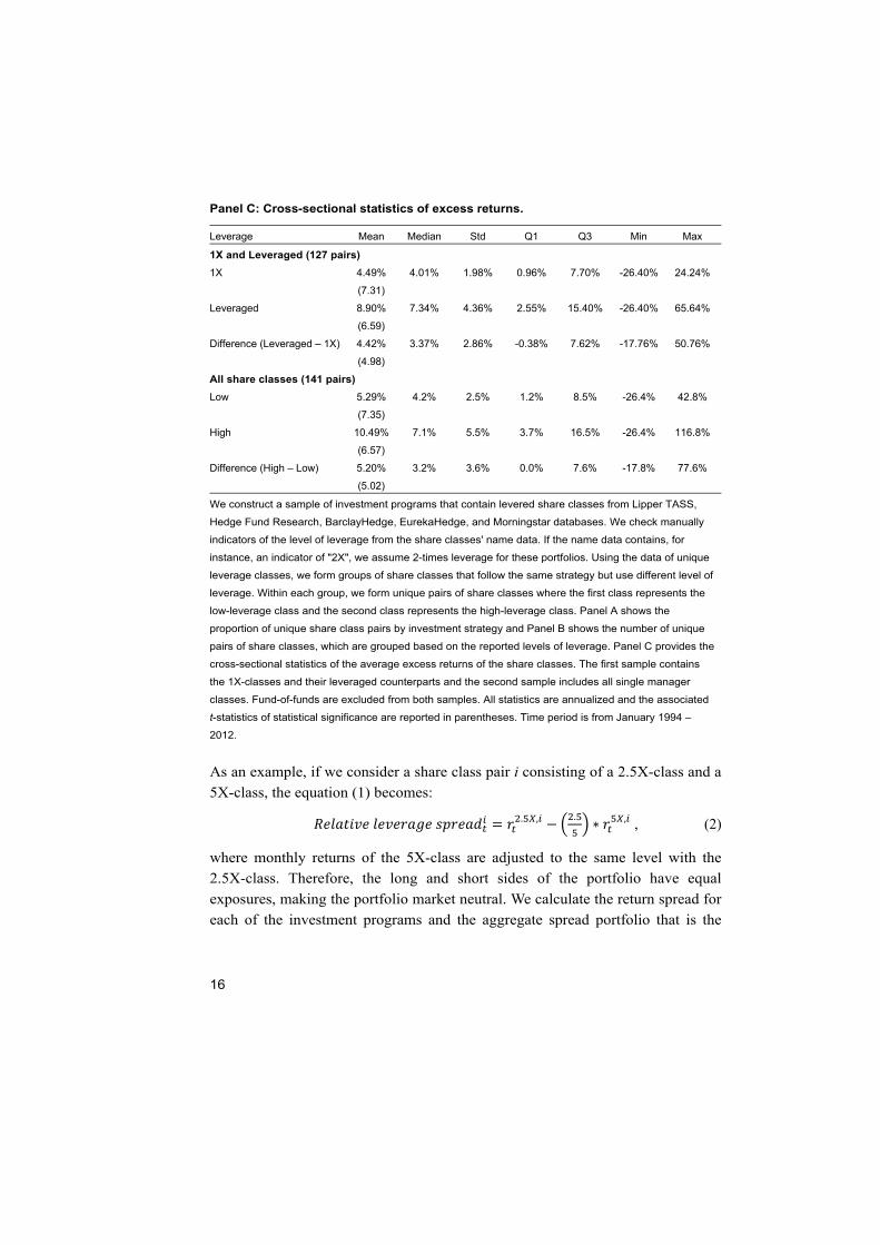
Panel C: Cross-sectional statistics of excess returns.

Leverage Mean Median Std Q1 Q3 Min Max

1X and Leveraged (127 pairs)

1X 4.49% 4.01% 1.98% 0.96% 7.70% -26.40% 24.24%

(7.31)

Leveraged 8.90% 7.34% 4.36% 2.55% 15.40% -26.40% 65.64%

(6.59)

Difference (Leveraged – 1X) 4.42% 3.37% 2.86% -0.38% 7.62% -17.76% 50.76%

(4.98)

All share classes (141 pairs)

Low 5.29% 4.2% 2.5% 1.2% 8.5% -26.4% 42.8%

(7.35)

High 10.49% 7.1% 5.5% 3.7% 16.5% -26.4% 116.8%

(6.57)

Difference (High – Low) 5.20% 3.2% 3.6% 0.0% 7.6% -17.8% 77.6%

(5.02)

We construct a sample of investment programs that contain levered share classes from Lipper TASS,

Hedge Fund Research, BarclayHedge, EurekaHedge, and Morningstar databases. We check manually

indicators of the level of leverage from the share classes' name data. If the name data contains, for

instance, an indicator of "2X", we assume 2-times leverage for these portfolios. Using the data of unique

leverage classes, we form groups of share classes that follow the same strategy but use different level of

leverage. Within each group, we form unique pairs of share classes where the first class represents the

low-leverage class and the second class represents the high-leverage class. Panel A shows the

proportion of unique share class pairs by investment strategy and Panel B shows the number of unique

pairs of share classes, which are grouped based on the reported levels of leverage. Panel C provides the

cross-sectional statistics of the average excess returns of the share classes. The first sample contains

the 1X-classes and their leveraged counterparts and the second sample includes all single manager

classes. Fund-of-funds are excluded from both samples. All statistics are annualized and the associated

t-statistics of statistical significance are reported in parentheses. Time period is from January 1994 –

2012.

As an example, if we consider a share class pair i consisting of a 2.5X-class and a

5X-class, the equation (1) becomes:

. , .∗ , , (2)

where monthly returns of the 5X-class are adjusted to the same level with the

2.5X-class. Therefore, the long and short sides of the portfolio have equal

exposures, making the portfolio market neutral. We calculate the return spread for

each of the investment programs and the aggregate spread portfolio that is the

17

equal-weighted and monthly rebalanced average of the individual strategy level

spread returns.

Intuitively, if managers are able to (and willing to) use leverage as their

investment programs suggest, the average performance of the aggregate spread

portfolio should be statistically indistinguishable from zero. According to the

alternative hypothesis, as predicted by the theory of leverage aversion (Frazzini &

Pedersen 2013), the aggregate spread return between low- and high-leverage classes

is positive and statistically significant after returns are adjusted for risk.

18

4 Performance and risk of leveraged share classes, 1994–2012

The idea in this study is to compare performance of the high-leverage share classes to

their low-leverage counterparts. We report statistics separately for the low- and high-

leverage classes as well as for the return difference between these two portfolios. In

this section, we measure the performance of the leveraged share classes without any

adjustment to their returns. Therefore this comparison allows us to examine the effect

of leverage on hedge fund returns and risk. Since the returns of the high-leverage

classes have higher exposure to market risk factors than their low-leverage

counterparts, we expect the high-leverage classes to generate higher returns.

4.1 Cross-sectional statistics

In Panel C of Table 1, we document the cross-sectional statistics of the leverage

classes. We document results for two samples. First, we report the cross-sectional

statistics of the average excess returns for the 1X-classes and their high-leverage

counterparts (127 pairs). Second, we report the cross-sectional statistics of the average

excess returns for all pairs of single-manager share classes (141 pairs). In both

samples, the high-leverage share classes have higher cross-sectional mean of the

average excess returns. In the second sample (141 pairs), the cross-sectional mean of

the average excess returns is 10.49% (t = 6.57) for the high-leverage classes whereas

it is 5.29% (t = 7.35) for the low-leverage classes. The cross-sectional average of the

spread performance is 5.20% (t = 5.02) which is economically and statistically

significant. Both samples provide similar results of the cross-sectional statistics.

Therefore, in rest of the paper, we use the sample that includes all fund class pairs.

4.2 Sorts

In performance evaluation, we follow previous studies and examine hedge funds'

alpha that is the value added of the strategy over passive and "mechanical"

benchmarks. It is important to adjust returns of fund classes to systematic risk in order

to control for the possibility that leverage magnifies the level of market risk. Our main

benchmark model specification for evaluating hedge fund risk-adjusted performance

is the Fung & Hsieh (2004) model. Formally, the model can be shown as:

19

, , , , , 3

where , is the excess return of the investment program (or a fund share class),

measures the abnormal return (FH Alpha), , is the beta risk loading of the factor k

during the time period, , is the factor return at time t, and , is the model's error

term. The seven factors included in the model are: the excess return of the S&P 500

index (SP – RF); the return spread between the Russell 2000 and the S&P 500 index

(RL – SP); the excess return of 10-year U.S. treasuries (TY – RF); the return of

Moody's BAA corporate bonds minus 10-year treasuries (BAA – TY); and the excess

return of the lookback straddles on bonds (PTFSBD); currencies (PTFSFX); and

commodities (PTFSCOM). 16 Returns of hedge funds are often non-normal with

positive or negative skewness and fat tailed distributions (excess kurtosis). Fung &

Hsieh (2001) argue that if hedge fund returns are non-normal, then lookback option-

based trend-following factors increase the model’s ability to explain return variation.

We construct equal-weighted (EW) portfolios of the low- and high-leverage share

classes. We also calculate the spread portfolio that is the return difference between the

high- and low-leverage portfolios. A monthly EW return of a portfolio is simply the

arithmetic average of share classes’ returns in that portfolio. Returns of portfolios are

therefore rebalanced monthly. The estimated FH alpha for the portfolios of low- and

high-leverage share classes implies performance of the average share class in those

portfolios and the alpha of the spread return measures whether the difference between

the two portfolios is economically and statistically significant.

Table 2 reports results of the average performance during the time period of 1994

– 2012 including measures of the average excess return and the standard deviation of

excess return, as well as the estimation results of the Fung & Hsieh (2004) model.

Panel A shows the baseline results. In Panel B, returns are adjusted for backfill-bias

by excluding the first 12 months of the return history from each share class. Results in

Panels A and B reveal that both high-and low-leverage portfolios provide statistically

significant risk-adjusted returns. In Panel A, the high-leverage portfolio provides an

impressive 14.79% alpha and its outperformance with respect to the low-leverage

portfolio is 8.69%. Panel B shows that outperformance of the high-leverage portfolio

16 We download returns of trend-following factors from the web page of David Hsieh (http://people.duke.edu/~dah7/). Fung & Hsieh (2004) model could be augmented using the Pastor & Stambaugh (2003) liquidity factor in order to capture potentially higher liquidity risk exposure in the high-leverage portfolios. The results of this paper are robust to this model specification.

20

is robust to the backfill-adjustment17 which has a small impact on the high- and low-

leverage portfolios (less than 1% per annum). Besides the higher risk-adjusted

performance, the high-leverage portfolio has a significantly higher systematic risk

than the low-leverage portfolio. In Panel A, the factor loadings on S&P 500 index

excess returns, bond, and trend-following factors are about two times higher in the

high-leverage portfolio. This makes sense considering the findings in Table 1 (Panel

B) which shows that a typical share class in the high-leverage portfolio is 2-times

levered. The high- and low-leverage portfolios have significant loadings to the

currency trend-following factor which is a return of the straddle strategy constructed

from various lookback currency options. A high beta to this option-based currency

return suggests that hedge funds take leveraged bets to exploit opportunities in

volatile foreign exchange markets. Despite the higher levels of a total risk and a beta

risk in the high-leverage portfolio, the outperformance of the portfolio is robust across

all performance measures.

Figure 1 plots the time-varying EW average excess returns (Panel A), the

standard deviation of excess returns (Panel B), and the Sharpe ratios (Panel C) of the

low- and high-leverage portfolios. All performance measures are annualized and

estimated in a 36-month rolling window. Consistent with Table 2, the high-leverage

portfolio outperforms consistently over time. However, the magnitude of this

outperformance has become much smaller during and after the recent financial crises.

17 The backfill bias (also known as instant history bias) occurs because hedge funds tend to start reporting performance after a period of a good performance, and that history of a good performance (or a backfill) may be incorporated into the database. Related literature (e.g., Malkiel & Saha 2005, Joenväärä et al. 2014a) shows that backfilled returns are upwardly biased.

21

Ta

ble

2. P

erf

orm

an

ce

of

lev

era

ged

cla

ss

es

.

Pa

ne

l A:

Ba

se

lin

e (

Nu

mb

er

of

sh

are

cla

ss

pa

irs

= 1

41

).

Leve

rage

A

vg.

Exc

ess

Ret

urn

Std

. E

xces

s

Ret

urn

Sha

rpe

Rat

io

FH

Alp

ha

SP

– R

F

RL

– S

P

TY

– R

F

BA

A –

TY

P

TF

SB

D

PT

FS

FX

P

TF

SC

OM

R

²

Low

6.

12%

5.

10%

1.

17

6.10

%

0.04

1 0.

049

0.08

3 0.

014

0.01

0 0.

022

0.01

4 0.

19

(5

.23)

(5

.52)

(1

.80)

(1

.80)

(1

.88)

(0

.28)

(1

.60)

(4

.32)

(1

.92)

Hig

h

14.8

4%

11.2

7%

1.30

14

.79%

0.

090

0.05

9 0.

170

0.05

2 0.

023

0.04

3 0.

033

0.16

(5

.74)

(5

.94)

(1

.76)

(0

.96)

(1

.72)

(0

.45)

(1

.61)

(3

.71)

(2

.05)

Spr

ead

(Hig

h –

Low

) 8.

72%

8.

69%

0.

049

0.01

0 0.

087

0.03

7 0.

013

0.02

1 0.

019

0.12

(5

.6)

(5.6

5)

(1.5

5)

(0.2

6)

(1.4

3)

(0.5

2)

(1.4

5)

(2.8

9)

(1.9

3)

22

Pa

ne

l B

: B

ac

kfi

ll-a

dju

ste

d (

Nu

mb

er

of

sh

are

cla

ss

pair

s =

10

3).

Leve

rage

A

vg.

Exc

ess

Ret

urn

Std

. E

xces

s

Ret

urn

Sha

rpe

Rat

io

FH

Alp

ha

SP

– R

F

RL

– S

P

TY

– R

F

BA

A –

TY

P

TF

SB

D

PT

FS

FX

P

TF

SC

OM

R

²

Low

4.

95%

4.

88%

1.

00

5.16

%

0.00

1 0.

021

0.03

4 0.

063

0.01

5 0.

020

0.01

1 0.

17

(4

.30)

(4

.62)

(0

.04)

(0

.79)

(0

.77)

(1

.26)

(2

.34)

(3

.94)

(1

.55)

Hig

h

13.5

1%

11.6

3%

1.15

14

.15%

0.

014

0.01

2 0.

068

0.12

3 0.

040

0.04

2 0.

021

0.14

(4

.93)

(5

.23)

(0

.26)

(0

.18)

(0

.63)

(1

.01)

(2

.54)

(3

.41)

(1

.22)

Spr

ead

(Hig

h –

Low

) 8.

56%

8.

99%

0.

013

-0.0

09

0.03

4 0.

060

0.02

5 0.

022

0.01

0 0.

11

(5

.00

)

(5

.22

) (0

.38

) (-

0.2

3)

(0.4

9)

(0.7

7)

(2.4

7)

(2.8

1)

(0.9

1)

We c

onst

ruct

tw

o p

ort

folio

s of fu

nd s

hare

cla

sse

s depe

ndin

g o

n the

ir le

vera

ge

. F

or

inst

an

ce,

if a

2X

-cla

ss is

co

mp

are

d t

o a

5X

-cla

ss w

ithin

a s

pe

cific

inve

stm

ent pro

gra

m, th

e 2

X-c

lass

be

longs

to the lo

w-le

vera

ge p

ort

folio

(L

ow

) and t

he 5

X-c

lass

belo

ng

s to

the h

igh-leve

rage p

ort

folio

(H

igh

). T

he

sp

rea

d r

etu

rn

(Hig

h –

Lo

w)

is the

diff

ere

nce

in r

etu

rns

betw

een t

he h

igh-

and lo

w-le

vera

ge p

ort

folio

s. T

his

table

sho

ws

the a

nnualiz

ed a

vera

ge e

xcess

retu

rn (

Avg

. E

xcess

Retu

rn),

the a

nnua

lized s

tan

dard

devi

atio

n o

f exc

ess

retu

rn (

Std

. E

xcess

Retu

rn),

and t

he a

nnualiz

ed F

un

g &

Hsi

eh (

2004)

alp

ha (

FH

Alp

ha)

and it

s

ass

oci

ate

d t

-sta

tistic

in p

are

nth

ese

s. T

he r

isk

loadin

gs

are

as

follo

ws:

exc

ess

retu

rn o

f th

e S

&P

500 in

dex

(SP

− R

F);

retu

rn s

pre

ad b

etw

een t

he R

uss

ell

20

00

ind

ex

an

d t

he

S&

P 5

00

ind

ex

(RL

− S

P);

exc

ess

re

turn

of

10

-ye

ar

Tre

asu

rie

s (T

Y −

RF

); r

etu

rn s

pre

ad

be

twe

en

Mo

od

y’s

BA

A c

orp

ora

te b

on

ds

an

d 1

0-y

ea

r

Tre

asu

rie

s (B

AA

− T

Y);

an

d e

xce

ss r

etu

rns

of

loo

k-b

ack

str

ad

dle

s o

n b

on

ds

(PT

FS

BD

), c

urr

en

cie

s (P

TF

SF

X),

an

d c

om

mo

diti

es

(PT

FS

CO

M),

an

d t

he

last

colu

mn is

th

e R

-sq

uare

d o

f th

e m

odel.

Panel A

show

s th

e b

ase

line r

esu

lts.

In P

anel B

, re

turn

s are

adju

sted for

back

fill-bia

s by

exc

ludin

g the first

12 m

onth

s of

retu

rn h

isto

ry fro

m e

ach

fund s

hare

cla

ss.

23

Fig. 1. Time-varying average performance of leverage classes. Three figures display

the time-varying performance measures of the low- and high-leverage classes.

Returns of the high-leverage share classes are not adjusted at the level of low-

leverage share classes. Reported are effects of leverage on the portfolios' excess

return (Panel A), FH alpha (Panel B), and the return per unit of risk ratio (Sharpe)

(Panel C).

Panel A: Excess returns.

Panel B: Fung & Hsieh (2004) alpha.

0%

5%

10%

15%

20%

25%

30%

35%

Dec-96 May-98 Oct-99 Mar-01 Aug-02 Jan-04 Jun-05 Nov-06 Apr-08 Sep-09 Feb-11 Jul-12

HighLow

0%

5%

10%

15%

20%

25%

30%

35%

40%

Dec-96 May-98 Oct-99 Mar-01 Aug-02 Jan-04 Jun-05 Nov-06 Apr-08 Sep-09 Feb-11 Jul-12

HighLow

24

Panel C: Sharpe ratio.

When the performance measure is a ratio of the average excess return per unit of

risk taken (Sharpe ratio), the high-leverage portfolio performance clearly

converges towards the low-leverage portfolio performance. We calculate the p-

value of the difference (using the procedure of Ledoit & Wolf 2008) in Sharpe

ratios between the low- and high-leverage portfolios and find that the difference

in Sharpe ratios is not statistically significant. Thus, the average performance

remains similar across the low- and high-leverage portfolios when average returns

are measured per unit of risk taken. When comparing share classes with different

levels of leverage, it makes sense to adjust average returns to volatility.

0

0,5

1

1,5

2

2,5

3

Dec-96 May-98 Oct-99 Mar-01 Aug-02 Jan-04 Jun-05 Nov-06 Apr-08 Sep-09 Feb-11 Jul-12

HighLow

25

5 Relative performance of leveraged fund share classes, 1994 – 2012

5.1 Cross-sectional statistics

We measure the difference in returns between low- and high-leverage portfolios as

defined in equation (1) in which the long and short sides of the relative leverage

spread portfolio have equal exposure which makes the spread portfolio market neutral

and balances the risk of the long and short sides. The spread return reflects the

discrepancy between getting market exposure using high-leverage strategies relative

to those of low-leverage strategies. The fundamental question is how to compare the

low- and high-levered returns. One potential measure in this purpose would be the

Treynor ratio statistic which divides excess returns by beta. In this study, we control

the systematic risk of the high-leverage funds by adjusting their returns to the same

level with their low-leverage counterparts.

We provide a case study of a CTA trading program which is managed by the

Ramsey Quantitative Systems, Inc. The program includes one 1X-class and one 2X-

class. Figure 2 (Panel A) shows the cumulative returns of (1) the 1X-class; (2) the 2X-

class with unadjusted returns; and (3) the 2X-class with adjusted returns by

multiplying each monthly return by 0.5. Panel B shows the cumulative RLS returns

measured as a return difference between the 1X-class and the adjusted 2X-class. Also

reported are the annualized arithmetic mean and the annualized standard deviation of

returns. Naturally, the unadjusted 2X-class outperforms the 1X-class (8.1% versus

4.9%) with 2-times higher volatility (6.4%*2 = 12.8%). The unadjusted 2X-class has

a slightly smaller risk/return tradeoff (Sharpe ratios are 0.63 versus 0.77), but it can

add value for the investor due to a higher total return. However, although the 2X-class

has provided two times higher volatility with leverage, the adjusted 2X-class does not

catch up with the performance of the 1X-class. The difference in the average returns

is 90 basis points between the 1X-class and the adjusted 2X-class. Investors may

benefit from the higher expected return of the 2X-class but not that much as expected.

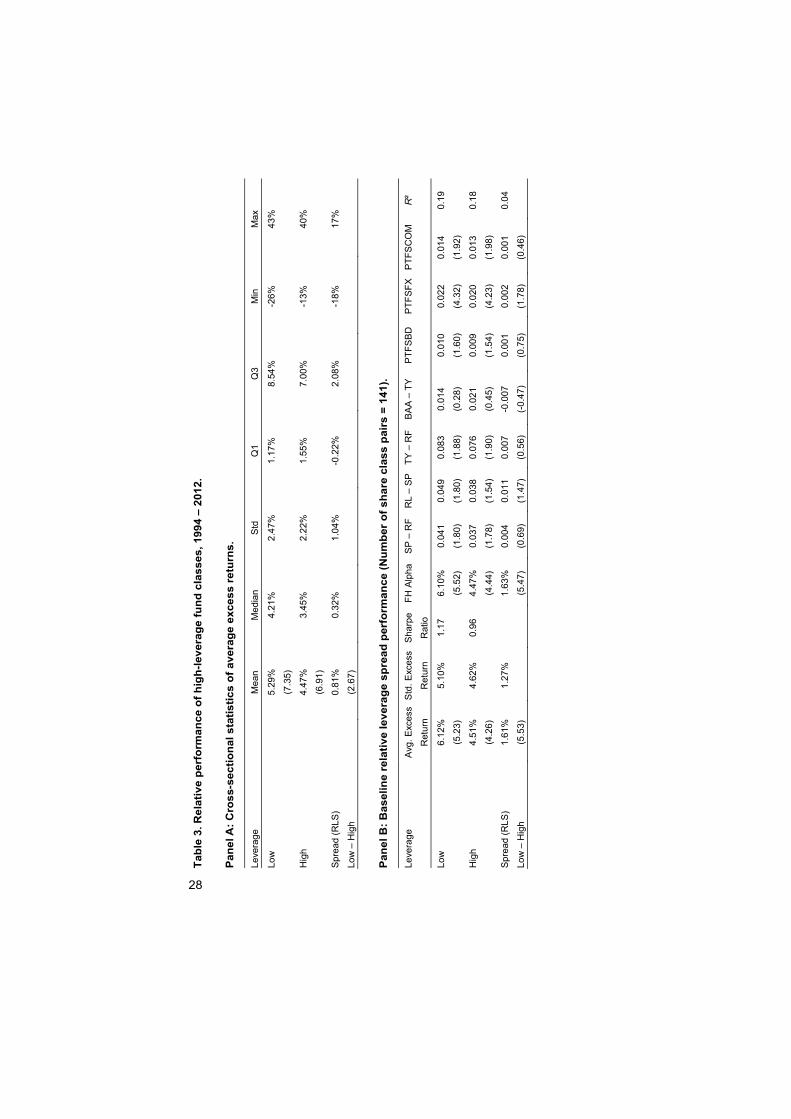
Panel A of Table 3 shows the cross-sectional statistics of the 141 low-and high-

leverage fund share classes as well as their spread performance. The high-leverage

share classes with adjusted returns have a lower cross-sectional mean of the average

excess returns. The cross-sectional mean of the individual strategies' average spread

returns is 0.81% (t = 2.67). This gives us first evidence that the leverage is associated

26

with low returns, as suggested by theory of leverage aversion (Frazzini & Pedersen

2013, Black 1972).

5.2 Sorts

Panels B and C of Table 3 provide further evidence from portfolio sorts. Panel B

shows the baseline results. In Panel C, returns are adjusted for the backfill-bias as in

Table 2. We report results for the EW RLS portfolio and its long and short sides. The

same return and risk measures are reported as in Table 2.

Consistent with theoretical predictions, the RLS portfolio generates statistically

significant average excess returns and FH alphas.18 In Panel B, the average excess

return (FH alpha) of the RLS portfolio is 1.61% (1.63%) with t-statistics above 5.

This result suggests that the return difference between the low-and high-leverage

share classes is statistically significant. The backfill-adjustment drops the average

RLS alpha to 1.07% (t = 3.84) but it is still statistically significant. The return

adjustment of the high-leverage classes shows that the factor loadings are close to the

low-leverage portfolios.

Figure 3 shows the time-varying average excess returns (Panel A) and the FH

alphas (Panel B) for RLS portfolios. As in Figure 1, estimates are measured in a 36-

month rolling window. Results show that the RLS portfolio has a positive

performance over time and during major crisis episodes including those of (1)

September 1998 – November 1998 (the LTCM episode); (2) August 2007 – October

2007 (the Quant crisis); and (3) September 2008 – November 2008 (the Subprime

crisis). During the last period of the sample (2009 – 2012), the RLS portfolio

performance has been moderate. Panel C of Figure 3 reveals that the low-leverage

portfolio outperforms the high-leverage portfolio also in terms of Sharpe ratios. The

performance of the low- and high-leverage portfolios has remained similar during the

years 2003 – 2006 and after 2010.

18 The RLS performance remains robust if additional trend-following factors are included to the Fung & Hsieh (2004) seven-factor factor model.

27

Fig. 2. Performance of individual CTA share classes, June 2003 – June 2010. This

figure shows performance of 1X- and 2X-classes of the CTA strategy managed by

Ramsey Quantitative Systems, Inc. Panel A shows the cumulative returns of (i) the 1X-

class; (ii) the 2X-class; and (iii) the 2X-class after its returns are adjusted at the same

level with the 1X-class. Also included are the average return and the standard

deviation of returns during June 2003 – June 2010. Panel B shows the cumulative

return difference between the 1X-class and the 2X-class with adjusted returns

(Relative leverage spread). The return difference corresponds to the return that

consists of a long position to the low-leverage share class (1X) and short position to

the high-leverage share class (2X) with adjusted returns.

Panel A: Cumulative simple returns of CTA share classes.

Panel B: Cumulative relative leverage spread (RLS).

0%

2%

4%

6%

8%

Jun-03 Apr-04 Feb-05 Dec-05 Oct-06 Sep-07 Jul-08 May-09 Mar-10

-10%

0%

10%

20%

30%

40%

50%

60%

70%

80%

90%

Jun-03 Apr-04 Feb-05 Dec-05 Oct-06 Sep-07 Jul-08 May-09 Mar-10

1X2X (Unadjusted Exposure)2X (Adjusted Exposure)

2X Unadjusted

(Mean=8.1% Std.=12.8%)

1X (Mean=4.9%

Std.=6.4%)

2X Adjusted (Mean=4.0%

Std.=6.4%)

28

Ta

ble

3. R

ela

tiv

e p

erf

orm

an

ce o

f h

igh

-le

ve

rag

e f

un

d c

las

se

s,

19

94

– 2

01

2.

Pa

ne

l A:

Cro

ss-s

ec

tio

nal

sta

tis

tic

s o

f a

ve

rag

e e

xc

es

s r

etu

rns

.

Leve

rage

M

ean

M

edia

n S

td

Q1

Q

3

Min

M

ax

Low

5.

29%

4.

21%

2.

47%

1.

17%

8.

54%

-2

6%

43%

(7

.35)

Hig

h 4.

47%

3.

45%

2.

22%

1.

55%

7.

00%

-1

3%

40%

(6

.91)

Spr

ead

(RLS

) 0.

81%

0.

32%

1.

04%

-0

.22%

2.

08%

-1

8%

17%

Low

– H

igh

(2

.67)

Pa

ne

l B

: B

as

elin

e r

ela

tiv

e l

ev

era

ge

sp

rea

d p

erf

orm

an

ce

(N

um

be

r o

f s

ha

re c

las

s p

air

s =

14

1).

Leve

rage

A

vg.

Exc

ess

Ret

urn

Std

. E

xces

s

Ret

urn

Sha

rpe

Rat

io

FH

Alp

ha

SP

– R

F

RL

– S

P

TY

– R

F

BA

A –

TY

P

TF

SB

D

PT

FS

FX

P

TF

SC

OM

R

²

Low

6.

12%

5.

10%

1.

17

6.10

%

0.04

1 0.

049

0.08

3 0.

014

0.01

0 0.

022

0.01

4 0.

19

(5

.23)

(5

.52)

(1

.80)

(1

.80)

(1

.88)

(0

.28)

(1

.60)

(4

.32)

(1

.92)

Hig

h

4.51

%

4.62

%

0.96

4.

47%

0.

037

0.03

8 0.

076

0.02

1 0.

009

0.02

0 0.

013

0.18

(4

.26)

(4

.44)

(1

.78)

(1

.54)

(1

.90)

(0

.45)

(1

.54)

(4

.23)

(1

.98)

Spr

ead

(RLS

)

1.61

%

1.27

%

1.

63%

0.

004

0.01

1 0.

007

-0.0

07

0.00

1 0.

002

0.00

1 0.

04

Low

– H

igh

(5.5

3)

(5.4

7)

(0.6

9)

(1.4

7)

(0.5

6)

(-0.

47)

(0.7

5)

(1.7

8)

(0.4

6)

29

Pa

ne

l C

: B

ac

kfi

ll-a

dju

ste

d r

ela

tiv

e l

ev

era

ge

sp

rea

d p

erf

orm

an

ce

(N

um

be

r o

f sh

are

cla

ss

pa

irs

= 1

03).

Leve

rage

A

vg.

Exc

ess

Ret

urn

Std

. E

xces

s

Ret

urn

Sha

rpe

Rat

io

FH

Alp

ha

SP

– R

F

RL

– S

P

TY

– R

F

BA

A –

TY

P

TF

SB

D

PT

FS

FX

P

TF

SC

OM

R

²

Low

4.

95%

4.

88%

1.

00

5.16

%

0.00

1 0.

021

0.03

4 0.

063

0.01

5 0.

020

0.01

1 0.

17

(4

.30)

(4

.62)

(0

.04)

(0

.79)

(0

.77)

(1

.26)

(2

.34)

(3

.94)

(1

.55)

Hig

h

3.85

%

4.64

%

0.82

4.

10%

-0

.003

0.

016

0.02

6 0.

068

0.01

5 0.

020

0.01

0 0.

17

(3

.52)

(3

.86)

(-

0.15

) (0

.64)

(0

.60)

(1

.43)

(2

.34)

(4

.09)

(1

.44)

Spr

ead

(RLS

)

1.09

%

1.11

%

1.

07%

0.

004

0.00

5 0.

009

-0.0

05

0.00

1 0.

000

0.00

1 0.

01

Low

– H

igh

(4.1

7)

(3.8

4)

(0.7

3)

(0.7

3)

(0.7

8)

(-0.

38)

(0.4

8)

(0.2

2)

(0.7

2)

We test

sta

tistic

ally

the d

iffere

nce

in r

etu

rns

betw

een lo

w-

and h

igh-le

vera

ge c

lass

es.

Retu

rns

of hig

h-leve

rage c

lass

es

are

ad

just

ed a

t th

e s

am

e le

vel w

ith

low

-leve

rag

e c

lass

es.

The r

ela

tive le

vera

ge s

pre

ad (

RL

S)

retu

rn o

f a s

hare

cla

ss p

air i

is

,∗

, ,

where

is

the r

etu

rn o

f th

e le

vera

ge c

lass

and in

dic

ato

r va

riable

s Lo

w a

nd H

igh r

efe

r to

the le

vel o

f le

vera

ge.

Th

e r

ela

tive le

vera

ge

spre

ad p

ort

folio

is

const

ruct

ed to b

e m

ark

et neutr

al w

ith r

etu

rn o

f each

hig

h-leve

rage c

lass

adju

sted a

t th

e le

vel o

f its

low

-leve

rage c

ounte

rpart

. P

anel A

show

s th

e c

ross

-

sect

ional s

tatis

tics

of th

e a

vera

ge e

xcess

retu

rns

of sh

are

cla

sse

s and P

an

el B

show

s re

sults

of ave

rage p

erf

orm

ance

for

the e

qu

al-w

eig

hte

d p

ort

folio

s. In

Panel C

, re

turn

s a

re a

dju

sted for

back

fill-bia

s by

exc

ludin

g the first

12 m

on

ths

of re

turn

his

tory

fro

m e

ach

share

cla

ss. P

anels

B a

nd

C r

ep

ort

th

e s

am

e r

etu

rn

and r

isk

measu

res

as

Table

2.

Fund-o

f-fu

nds

are

exc

luded f

rom

the s

am

ple

.

30

Fig. 3. Time-varying average relative performance of high-leverage fund share classes.

This figure displays the time-varying performance of the low-leverage and the high-

leverage portfolios as well as their return difference (RLS). The returns of the high-

leverage classes are adjusted at the same level with their low-leverage counterparts.

All performance measures are annualized. Fund-of-funds are excluded.

Panel A: Excess returns.

Panel B: Fung & Hsieh (2004) alphas.

-1%

0%

1%

2%

3%

4%

5%

6%

7%

0%

2%

4%

6%

8%

10%

12%

14%

Dec-96 May-98 Oct-99 Mar-01 Aug-02 Jan-04 Jun-05 Nov-06 Apr-08 Sep-09 Feb-11 Jul-12

Relative Leverage SpreadLow and High Leverage

Relative Leverage Spread (RLS)LowHigh

-1%

0%

1%

2%

3%

4%

5%

0%

2%

4%

6%

8%

10%

12%

14%

16%

18%

Dec-96 May-98 Oct-99 Mar-01 Aug-02 Jan-04 Jun-05 Nov-06 Apr-08 Sep-09 Feb-11 Jul-12

Low and High Leverage Relative Leverage Spread

Relative Leverage Spread (RLS)LowHigh

31

Panel C: Sharpe ratio.

5.3 Robustness

We test the robustness of the RLS performance using a sample that also includes

fund-of-funds for the time period of January 1994 – December 2012. Portfolio sorts in

Table 4 reveal similar RLS performance as in Table 3. Specifically, the RLS alpha is

1.84% with the t-statistic equaling to 6.21. The underperformance of the scaled high-

leverage portfolio is robust to addition of fund-of-funds.

Furthermore, we examine the robustness of the RLS performance during the time

periods of financial distress and major crisis periods, and report results in Table 5.

First, we approximate “flight-to-liquidity” periods as months when (i) the VIX

volatility index has been above its historical median value; (ii) and when the S&P 500

index excess return has been below its historical median. Second, we report the

average returns of RLS portfolios during three important crisis periods: (i) the LTCM

episode; (ii) the Quant crisis; and (iii) the Subprime crisis. During the flight-to-

liquidity periods, the average return of the RLS portfolio is 1.70% (t = 3.04) whereas

it is 1.55% (t = 4.72) after the flight-to-liquidity periods are excluded. During the

financial crisis episodes, we find insignificant average return for the RLS portfolio.

However, the average performance during the financial crisis periods is calculated

using nine return observations referring to small statistical power in analysis. We

conclude that the RLS performance is not driven by specific crisis episodes.

0,0

0,5

1,0

1,5

2,0

2,5

3,0

Dec-96 May-98 Oct-99 Mar-01 Aug-02 Jan-04 Jun-05 Nov-06 Apr-08 Sep-09 Feb-11 Jul-12

LowHigh

32

Ta

ble

4. R

ob

ustn

es

s o

f R

LS

pe

rfo

rman

ce

wit

h f

un

d-o

f-fu

nd

s, 1

99

4 –

20

12

.

Leve

rage

A

vg.

Exc

ess

Ret

urn

Std

. E

xces

s

Ret

urn

Sha

rpe

Rat

io

FH

Alp

ha

SP

– R

F

RL

– S

P

TY

– R

F

BA

A –

TY

P

TF

SB

D

PT

FS

FX

P

TF

SC

OM

R

²

Low

6.

05%

4.

99%

1.

18

5.61

%

0.06

3 0.

045

0.08

2 0.

081

0.00

7 0.

021

0.01

3 0.

17

(

5.28

)

(5

.14)

(2

.82)

(1

.68)

(1

.88)

(1

.60)

(1

.09)

(4

.04)

(1

.78)

Hig

h

4.15

%

4.49

%

0.91

3.

78%

0.

056

0.03

3 0.

069

0.07

8 0.

006

0.01

8 0.

012

0.17

(

4.03

)

(3

.83)

(2

.80)

(1

.37)

(1

.77)

(1

.69)

(1

.15)

(3

.92)

(1

.84)

Spr

ead

(RLS

) 1.

90%

1.

26%

1.84

%

0.00

7 0.

012

0.01

2 0.

004

0.00

0 0.

003

0.00

1 0.

04

Low

– H

igh

(6.

57)

(6.2

1)

(1.0

8)

(1.6

4)

(1.0

5)

(0.2

6)

(0.1

8)

(1.8

6)

(0.4

4)

This

table

sh

ow

s re

sults

of

the a

vera

ge p

erf

orm

ance

of

the R

LS

port

folio

after

fund-o

f-fu

nds

are

incl

uded t

o t

he d

ata

. T

he R

LS

port

folio

is c

onst

ruct

ed a

s in

Table

3. A

ll equal-

weig

hte

d p

ort

folio

s in

clude 1

76 p

airs

of sh

are

cla

sses.

Tim

e p

eriod is

Jan

uary

1994 –

Dece

mber

2012.

33

Table 5. RLS performance during "flight-to-liquidity" periods and financial crisis

episodes.

Average Excess Returns

Flight-to-Liquidity

Periods

Other Periods Financial Crisis Periods Other Periods

Observations 82 146 9 219

Low 4.26% 7.16% 13.20% 5.83%

(2.3) (4.78) (2.03) (4.91)

High 2.56% 5.62% 11.93% 4.21%

(1.59) (4.05) (1.99) (3.92)

Spread (RLS) 1.70% 1.55% 1.24% 1.62%

Low – High (3.04) (4.72) (0.98) (5.44)

This table shows the average excess returns of the equal-weighted RLS factor during the "flight-to-

liquidity" periods and financial crisis episodes. We measure the flight-to-liquidity periods as follows: (i) the

monthly return of the VIX volatility index is above its historical median; and (ii) the S&P 500 monthly

return is below its historical median. We select the following months as financial crisis episodes: (1)

LTCM episode (September 1998 – November 1998); (2) Quant crisis (August 2007 – October 2007); and

(3) Subprime crisis (September 2008 – November 2008). The associated t-statistics of the average

excess returns are reported in parentheses. All fund-of-funds are excluded.

5.4 Fees

Multiple leverage classes within investment programs typically charge the same

management and performance-based fees. Intuitively, depending on performance, the

use of leverage in an investment program may result in higher (lower) incentive fees

for the manager, if leverage magnifies the fund’s value above (below) the high-

watermark. If managers are willing to decrease the level of leverage (or are forced to

do so) especially during stress periods, this would decrease the impact of fees on

returns (Dai & Sundaresan 2010). If the high-leverage classes charge higher incentive

fees than the low-leverage classes, this should be reflected positively to RLS

performance.

We test this prediction with gross returns using the methodology as proposed by

Brooks et al. (2007).19 Portfolio sorts are repeated for share class portfolios with

estimated gross returns and we are left with 134 unique pairs of leverage classes.

Table 6 summarizes the results. Panel A (Panel B) shows the results of sorts for net-

of-fees (gross-of-fees) returns. The RLS portfolio’s gross-of-fees alpha is even larger

19 Their algorithm requires that the management fee and the incentive fees of funds are non-missing in admin modules.

34

than the net-of-fees alpha. In Panel B, the average class in the high-leverage portfolio

has 2.69% lower FH alphas than the average class in the low-leverage portfolio. The

t-statistic (7.5) indicates that the difference in alphas is statistically significant. Since

the gross-of-fees alpha of the RLS portfolio is higher than the net-of-fees alpha, it

indicates that fees have larger impact on returns of low-leverage classes. Thus, these

findings suggest that the asymmetric performance fees do not drive the RLS

performance.

5.5 Time series regressions

Liu & Mello (2011) model theoretically how the fragile nature of the capital structure

in hedge funds combined with imperfect market liquidity hampers funds’ ability to

perform market arbitrage. The fragile equity capital in hedge funds introduces the risk

of coordination among hedge fund investors. The coordination risk arises because

investors suspect that other investors might redeem, and to meet redemptions the fund

may be forced to liquidate positions at a loss. Both the equity and the debt of hedge

funds are fragile since they can be withdrawn on short notice by investors.

The model of Liu & Mello (2011) predicts that the fragile nature of the equity

(and debt) in hedge funds creates an effective market-disciplining mechanism. It

induces hedge funds to behave conservatively, by holding less risky portfolios and

operating with less leverage. Therefore, hedge funds may adjust their level of

leverage based on the costs of leverage.

We test the possibility that the RLS performance is driven by the changes in

borrowing costs. Intuitively, it would be optimal for the manager to adjust the level of

leverage based on the costs of borrowing. For instance, during a financial crisis, when

borrowing costs are likely to be high, hedge funds may decrease their leverage.

We test exposures of the RLS portfolio to various proxies of borrowing costs. We

use the following proxies:

1. Monthly change in the constant maturity 3-month T-bill rate (∆(level));

2. Return to the slope of the yield curve, measured by the yield spread between

the 10-year Treasury rate and the 3-month T-bill rate (∆(Slope))20;

20 Patton and Ramadorai (2013) use ∆(level) and ∆(Slope) as proxies of borrowing costs.

35

Ta

ble

6. G

ros

s p

erf

orm

an

ce

of

RL

S p

ort

foli

o,

19

94

– 2

01

2.

Pa

ne

l A:

Net-

of-

fee

s r

etu

rns

.

Leve

rage

A

vg.

Exc

ess

Ret

urn

Std

. E

xces

s

Ret

urn

Sha

rpe

Rat

io

FH

Alp

haS

P –

RF

R

L –

SP

T

Y –

RF

B

AA

– T

Y

PT

FS

BD

P

TF

SF

X

PT

FS

CO

M

R²

Low

5.

97%

5.

02%

1.

16

5.93

%

0.04

2 0.

047

0.08

1 0.

016

0.01

0 0.

021

0.01

3 0.

18

(5

.18)

(5

.41)

(1

.88)

(1

.72)

(1

.86)

(0

.32)

(1

.67)

(4

.15)

(1

.82)

Hig

h 4.

45%

4.

51%

0.

97

4.39

%

0.04

0 0.

036

0.07

1 0.

023

0.00

9 0.

019

0.01

2 0.

18

(4

.29)

(4

.45)

(1

.96)

(1

.48)

(1

.83)

(0

.51)

(1

.69)

(4

.11)

(1

.89)

Spr

ead

(RLS

) 1.

52%

1.

27%

1.53

%

0.00

3 0.

011

0.00

9 -0

.007

0.

001

0.00

2 0.

001

0.04

Low

– H

igh

(5.2

2)

(5.1

2)

(0.4

4)

(1.4

2)

(0.7

9)

(-0.

50)

(0.5

5)

(1.6

4)

(0.4

2)

Pa

ne

l B

: G

ros

s-o

f-fe

es

re

turn

s.

Leve

rage

A

vg.

Exc

ess

Ret

urn

Std

. E

xces

s

Ret

urn

Sha

rpe

Rat

io

FH

Alp

ha

SP

– R

F

RL

– S

P

TY

– R

F

BA

A –

TY

P

TF

SB

D

PT

FS

FX

P

TF

SC

OM

R

²

Low

10

.22%

5.

95%

1.

68

10.2

1%

0.05

0 0.

055

0.09

2 0.

006

0.01

3 0.

024

0.01

4 0.

17

(7

.48)

(7

.83)

(1

.89)

(1

.69)

(1

.77)

(0

.09)

(1

.72)

(3

.98)

(1

.70)

Hig

h 7.

54%

5.

21%

1.

42

7.52

%

0.04

4 0.

045

0.07

7 0.

016

0.01

1 0.

022

0.01

3 0.

17

(6

.3)

(6.5

8)

(1.8

9)

(1.5

9)

(1.7

0)

(0.3

0)

(1.6

9)

(4.0

4)

(1.7

8)

Spr

ead

(RLS

) 2.

68%

1.

53%

2.69

%

0.00

6 0.

010

0.01

5 -0

.010

0.

002

0.00

3 0.

001

0.04

Low

– H

igh

(7.6

7)

(7.5

0)

(0.8

4)

(1.0

9)

(1.0

5)

(-0.

61)

(0.8

7)

(1.6

1)

(0.4

9)

This

table

sh

ow

s th

e e

qual-w

eig

hte

d R

LS

port

folio

perf

orm

ance

usi

ng g

ross

retu

rns

of le

vera

ge c

lass

es.

Gro

ss r

etu

rns

are

est

ima

ted a

s pro

pose

d b

y B

rooks

et al.

(2007).

We c

onst

ruct

port

folio

s as

in T

able

3.

Pan

el A

show

s re

sults

for

the n

et-

of-

fees

retu

rns

and P

anel B

show

s re

sults

fo

r th

e g

ross

-of-

fee

s re

turn

s. I

n

Panels

A a

nd B

, th

e s

am

ple

incl

udes

134 u

niq

ue p

airs

of

leve

rage c

lass

es.

36

3. The return of Moody’s BAA corporate bonds minus 10-year treasuries (Credit

Spread);

4. TED spread (the 3-month LIBOR rate minus the 3-month T-bill rate) (TED);

5. Value-weighted return of all CRSP firms minus the 1-month T-bill rate (MKT

– RF);

6. Carry trade return of the developed countries' currencies net of transaction

costs (Carry Trade).21

7. VIX straddle return (VIX).

Using the EW portfolios of fund share classes and the proxies of potential costs of

leverage, we estimate the following time series regression using OLS:

α ∑ , , 4

where is the EW portfolio return at time t, is the model’s intercept, is the

sensitivity of the portfolio returns to the proxy k, which is measured at time t ( , , and is the model’s error term.

Table 7 shows the OLS estimation results of the time series regressions for the

monthly EW low- and high-leverage portfolios as well as the spread portfolio

measured as the return difference between the portfolios of low- and high-leverage

share classes. Table reports parameter estimates and their associated t-statistics in

parentheses. In order to examine the effects of leverage on the sensitivities of

portfolio returns to the proxies of borrowing costs, we do not adjust the returns of

high-leverage share classes at the same level with their low-leverage counterparts.

Panels A and B reveal that the portfolios of low- and high-leverage fund share classes

have negative loadings on the ∆(level), ∆(Slope), and the credit spread proxies. In

Panel A, the estimated coefficients of the change in the slope (∆(Slope)) are negative

and statistically significant across model specifications. In the Model 7, for instance,

the estimated loading on the ∆(Slope) is -0.936 (t = -2.50). Therefore, on average, a

one percent increase in the ∆(Slope) has a one percent impact on the EW return of

low-leverage share classes. The portfolio of high-leverage share classes has

considerably higher sensitivities to the proxies of borrowing costs if compared to the

portfolio of low-leverage share classes. For instance, for the portfolio of high-leverage

classes (Panel B), the Model 7 shows that the estimated loading on the ∆(Slope) is -

2.132 (t = -2.57). Panel C, which shows estimation results for the spread returns

between the portfolios of low- and high-leverage classes, confirms that the high-

21 We download the CRSP index return from the Ken French web page. The carry trade factor is from the Hanno Lustig’s web page.

37

leverage portfolio has higher sensitivities to the proxies of borrowings costs.

Nevertheless, the ∆(Slope) is the only proxy that has a statistically significant loading

in regressions. Overall, the ability of the model to explain return behavior of EW

portfolios is negligible. The R² values are small across model specifications.

Table 8 reports the results for the portfolios of low-leverage share classes and

high-leverage share classes, whose returns are adjusted at the same level with their

low-leverage counterparts. Also reported are the estimation results for the RLS factor.

As the Model 7 in Panels A and B suggests, the estimated coefficients of ∆(level)

and ∆(Slope) are negative and statistically significant. The portfolio of high-leverage

share classes has similar estimated coefficients with the portfolio of low-leverage

share classes since the returns of high-leverage classes are adjusted at the same level

with their low-leverage counterparts. The finding is confirmed in Panel C showing

that none of the proxies reveal statistically significant differences between the

portfolios of low- and high-leverage share classes.22 The R² values are small across

model specifications and the ability of time series regressions to explain the return

behavior of EW portfolios seems negligible. In Panel C the estimated intercepts are

positive and statistically significant across model specifications. Thus we conclude

that the result of the positive RLS performance seems not to be explained by the main

proxies of borrowing costs.23 As suggested in Figure 3, the RLS performance is robust

during the study period of 1994 – 2012.

22 This finding remains robust if we use time series regressions having independent variables, which are lagged by one month. 23 In robustness checks which are not reported for reasons of space, we examine whether there is a nonlinear relation between the different proxies of borrowing costs and returns from the RLS factor. We sort the cost proxies into deciles and then examine the spread in the returns on the RLS factor. We find no evidence that the extreme deciles (0 or 10) would provide higher average returns for the RLS factor. The similar result is obtained if the cost proxies are sorted into quintiles.

38

Table 7. Estimation results of time series regressions for equal-weighted portfolios,

1994 – 2012.

Panel A: Low leverage.

Variable [1] [2] [3] [4] [5] [6] [7]

Intercept 0.005 0.005 0.005 0.005 0.005 0.005 0.005

(5.16) (5.09) (5.04) (3.16) (3.05) (2.83) (2.89)

∆(Level) -0.472 -1.1 -1.071 -1.101 -1.117 -1.159 -1.151

(-1.12) (-2.25) (-2.01) (-2.01) (-2.05) (-2.12) (-2.10)

∆(Slope) -0.891 -0.88 -0.873 -0.92 -0.938 -0.936

(-2.47) (-2.37) (-2.34) (-2.46) (-2.51) (-2.50)

Credit Spread -0.007 -0.012 -0.039 -0.053 -0.056

(-0.14) (-0.22) (-0.66) (-0.87) (-0.92)

TED -0.001 -0.001 0.000 0.000

(-0.26) (-0.19) (0.00) (-0.03)

MKT – RF 0.029 0.021 0.011

(1.23) (0.87) (0.35)

Carry Trade 0.045 0.043

(1.23) (1.16)

VIX -0.004

(-0.60)

R² 0.005 0.032 0.032 0.032 0.039 0.045 0.047

Panel B: High leverage (Unadjusted returns).

Variable [1] [2] [3] [4] [5] [6] [7]

Intercept 0.012 0.012 0.012 0.011 0.011 0.01 0.01

(5.69) (5.62) (5.57) (3.04) (2.92) (2.71) (2.73)

∆(Level) -0.444 -1.851 -1.775 -1.708 -1.747 -1.833 -1.823

(-0.47) (-1.71) (-1.5) (-1.41) (-1.45) (-1.52) (-1.50)

∆(Slope) -1.997 -1.967 -1.984 -2.098 -2.134 -2.132

(-2.50) (-2.40) (-2.40) (-2.53) (-2.58) (-2.57)

Credit Spread -0.019 -0.008 -0.074 -0.101 -0.106

(-0.16) (-0.07) (-0.57) (-0.76) (-0.79)

TED 0.002 0.002 0.003 0.003

(0.27) (0.35) (0.52) (0.50)

MKT – RF 0.07 0.054 0.04

(1.34) (1.00) (0.59)

Carry Trade 0.093 0.09

(1.14) (1.09)

VIX -0.006

(-0.37)

R² 0.001 0.028 0.028 0.028 0.036 0.042 0.042

39

Panel C: Spread (High leverage – Low leverage).

Variable [1] [2] [3] [4] [5] [6] [7]

Intercept 0.007 0.007 0.007 0.006 0.006 0.005 0.005

(5.58) (5.50) (5.45) (2.67) (2.56) (2.38) (2.36)

∆(Level) 0.029 -0.751 -0.704 -0.607 -0.63 -0.674 -0.671

(0.05) (-1.15) (-0.99) (-0.83) (-0.86) (-0.92) (-0.92)

∆(Slope) -1.106 -1.088 -1.111 -1.178 -1.196 -1.196

(-2.29) (-2.19) (-2.23) (-2.36) (-2.39) (-2.38)

Credit Spread -0.012 0.004 -0.035 -0.049 -0.05

(-0.17) (0.05) (-0.44) (-0.61) (-0.62)

TED 0.002 0.003 0.003 0.003

(0.65) (0.72) (0.86) (0.85)

MKT – RF 0.041 0.033 0.029

(1.29) (1.00) (0.71)

Carry Trade 0.048 0.047

(0.96) (0.94)

VIX -0.001

(-0.16)

R² 0.000 0.023 0.023 0.025 0.032 0.036 0.036

We test sensitivity of returns of the portfolios of low- and high-leverage fund share classes to changes in

variables that capture the costs of borrowing. We use the following proxies: (1) Monthly change in the constant

maturity 3-month T-bill rate (∆(Level)); (2) The return to the slope of the yield curve, measured by the yield

spread between 10-year Treasury rate and the 3-month T-bill rate (∆(Slope)); (3) The credit spread between

BAA rated bonds and the 10-year Treasury rate (Credit Spread); (4) TED spread (the 3-month LIBOR rate

minus the 3-month T-bill rate) (TED); (5) Value-weighted return of all CRSP firms minus the 1-month Treasury

bill rate (MKT – RF); (6) Carry trade return of the developed countries' currencies net of transaction costs

(Carry Trade); and (7) VIX returns (VIX). We run a time series regression for the portfolios of low-leverage

(Panel A) and high-leverage (Panel B) share classes against the proxies of borrowing costs using OLS. We

also run a time series regression for the spread returns measured as the return difference between the

portfolios of low- and high-leverage share classes. All independent variables are contemporaneously

measured. The t-statistics of estimated coefficients are reported in parentheses.

40

Table 8. Estimation results of time series regressions for equal-weighted RLS

portfolio, 1994 – 2012.

Panel A: Low leverage.

Variable [1] [2] [3] [4] [5] [6] [7]

Intercept 0.005 0.005 0.005 0.005 0.005 0.005 0.005

(5.16) (5.09) (5.04) (3.16) (3.05) (2.83) (2.89)

∆(Level) -0.472 -1.100 -1.071 -1.101 -1.117 -1.159 -1.151

(-1.12) (-2.25) (-2.01) (-2.01) (-2.05) (-2.12) (-2.10)

∆(Slope) -0.891 -0.880 -0.873 -0.920 -0.938 -0.936

(-2.47) (-2.37) (-2.34) (-2.46) (-2.51) (-2.50)

Credit Spread -0.007 -0.012 -0.039 -0.053 -0.056

(-0.14) (-0.22) (-0.66) (-0.87) (-0.92)

TED -0.001 -0.001 0.000 0.000

(-0.26) (-0.19) (0.00) (-0.03)

MKT – RF 0.029 0.021 0.011

(1.23) (0.87) (0.35)

Carry Trade 0.045 0.043

(1.23) (1.16)

VIX -0.004

(-0.60)

R² 0.005 0.032 0.032 0.032 0.039 0.045 0.047

Panel B: High leverage (Adjusted returns).

Variable [1] [2] [3] [4] [5] [6] [7]

Intercept 0.004 0.004 0.004 0.004 0.004 0.004 0.004

(4.20) (4.11) (4.06) (2.61) (2.50) (2.28) (2.35)

∆(Level) -0.369 -0.933 -0.925 -0.954 -0.969 -1.007 -1.000

(-0.96) (-2.10) (-1.91) (-1.93) (-1.96) (-2.03) (-2.01)

∆(Slope) -0.801 -0.798 -0.791 -0.835 -0.851 -0.849

(-2.45) (-2.37) (-2.34) (-2.46) (-2.51) (-2.50)

Credit Spread -0.002 -0.007 -0.032 -0.044 -0.047

(-0.04) (-0.13) (-0.60) (-0.81) (-0.86)

TED -0.001 -0.001 0.000 0.000

(-0.29) (-0.21) (-0.02) (-0.05)

MKT – RF 0.027 0.020 0.010

(1.25) (0.89) (0.35)

Carry Trade 0.041 0.039

(1.23) (1.16)

VIX -0.004

(-0.64)

R² 0.004 0.030 0.030 0.030 0.037 0.044 0.045

41

Panel C: Relative leverage spread (RLS).

Variable [1] [2] [3] [4] [5] [6] [7]

Intercept 0.001 0.001 0.001 0.001 0.001 0.001 0.001

(5.47) (5.41) (5.39) (3.18) (3.12) (3.01) (2.98)

∆(Level) -0.103 -0.167 -0.146 -0.147 -0.148 -0.152 -0.152

(-0.98) (-1.36) (-1.09) (-1.07) (-1.08) (-1.10) (-1.09)

∆(Slope) -0.090 -0.082 -0.082 -0.085 -0.087 -0.087

(-0.99) (-0.88) (-0.87) (-0.91) (-0.92) (-0.92)

Credit Spread -0.005 -0.005 -0.007 -0.009 -0.009

(-0.39) (-0.37) (-0.49) (-0.56) (-0.56)

TED 0.000 0.000 0.000 0.000

(-0.02) (0.00) (0.07) (0.06)

MKT – RF 0.002 0.002 0.001

(0.39) (0.26) (0.16)

Carry Trade 0.004 0.004

(0.44) (0.43)

VIX 0.000

(-0.08)

R² 0.004 0.009 0.009 0.009 0.010 0.011 0.011

We test the sensitivity of RLS performance to changes in variables that capture the costs of borrowing. We

use the same independent variables as in Table 7. We run a time series regression for the portfolios of low-

leverage share classes (Panel A) and high-leverage share classes (Panel B) against the proxies of borrowing

costs using OLS. The returns of high-leverage share classes are adjusted to the same level with their low-

leverage counterparts. Panel C reports estimation results for the RLS portfolio. All independent variables are

contemporaneously measured. The t-statistics of estimated coefficients are reported in parentheses.

42

6 Conclusions

This study builds on the theoretical work of leverage aversion and margin constraints.

Using a hand-collected data on levered fund share classes from the union of major

commercial databases, we document that the share classes with high leverage exhibit

higher risk-adjusted returns, a systematic risk, and higher volatility than their low-

leverage counterparts. We find that the average low- and high-leverage share class

generates an economically and statistically significant FH alpha, which is in line with

previous literature suggesting that hedge funds add value for their investors.

The main finding of this study is that the average high-leverage share class

underperforms its low-leverage counterpart for the same investment program after

their returns are appropriately adjusted to the same level. More specifically, a relative

leverage spread (RLS) portfolio with long low-leverage share classes and short high-

leverage share classes generates significant risk-adjusted performance. During the

time period January 1994 – December 2012, the RLS portfolio of single manager

share classes generates a 1.63% FH alpha which is statistically significant. The result

is robust to the inclusion of fund-of-funds, sub periods, and gross returns. We also

document that the general proxies of the cost of leverage do not have any significant

explanatory power in explaining RLS returns.

The results of this study mirror the theoretical predictions of Frazzini & Pedersen

(2013) and Dai & Sundaresan (2010) suggesting that leverage aversion has an impact

on hedge fund performance. Therefore, investors may receive higher total returns by

investing in share classes with high-leverage. However, the RLS performance

indicates that investors do not receive benefits from high leverage as much as

suggested.

Our results imply that buying hedge funds with high leverage embedded in their

strategies increases investors' market exposure and value added without violating their

leverage constraints. Pension funds, for instance, which can be leverage-constrained

investors, can exploit leverage, which is embedded in fund share classes. Careful

monitoring of the hedge funds’ level of leverage and their exposures to market risk

factors is expected to add value.

This study examines the theoretical predictions of leverage aversion by exploiting

the monthly returns of fund share classes with various levels of leverage. The

examination of these theoretical predictions using the security-level data of the

management companies’ use of derivatives would be an interesting extension to this

study.

43

References

Ang A, Gorovyy S & van Inwegen GB (2011) Hedge fund leverage. Journal of Financial Economics 102(1): 102–126.

Asness CS, Frazzini A & Pedersen LH (2012) Leverage aversion and risk parity. Financial Analyst Journal 68(1): 47–59.

Black F (1972) Capital market equilibrium with restricted borrowing. Journal of Business 45(3): 444–455.

Black F, Jensen MC & Scholes M (1972) The capital asset pricing model: Some empirical tests. In: Jensen MC (ed.) Studies in the theory of capital markets. New York, Praeger: 79–121.

Breuer P (2000) Measuring off-balance-sheet leverage. Working paper. International Monetary Fund.

Brooks C, Clare A & Motson N (2007) The gross truth about hedge fund performance and risk: The impact of incentive fees. Working paper. University of Reading, City University London - Sir John Cass Business School.

Brown SJ, Goetzmann WN & Ibbotson RG (1999) Offshore hedge funds: Survival and performance, 1989–1995. Journal of Business 72(1): 91–118.

Buraschi A, Kosowski R & Stritrakul W (2013) Incentives and endogenous risk taking: A structural view of hedge fund alphas. Journal of Finance. Forthcoming.

Chen Y (2011) Derivatives use and risk taking: Evidence from the hedge fund industry. Journal of financial and quantitative analysis 46(4): 1073–1106.

Dai J & Sundaresan S (2010) Risk management framework for hedge funds: Role of funding and redemption options on leverage. Working paper. Columbia University.

Frazzini A & Pedersen LH (2013) Betting against beta. Journal of Financial Economics. Forthcoming.

Frazzini A & Pedersen LH (2012) Embedded leverage. NBER working paper no. w18558. Fung W, Hsieh DA, Naik NY & Ramadorai T (2008) Hedge funds: Performance, risk, and

capital formation. Journal of Finance 63(4): 1777–1803. Fung W & Hsieh DA (2004) Hedge fund benchmarks: A risk based approach. Financial

Analyst Journal 60(5): 65–80. Fung W & Hsieh DA (2001) The risk in hedge fund strategies: Theory and evidence from

trend followers. Review of Financial Studies 14(2): 313–341. Gârleanu N & Pedersen LH (2011) Margin-based asset pricing and deviations from the law

of one price. Review of Financial Studies 24(6): 1980–2022. Goetzmann WN, Ingersoll JE & Ross SA (2003) High-water marks and hedge fund

management contracts. Journal of Finance 58(4): 1685–1718. Jacobs BI & Levy K (2013) Leverage aversion, efficient frontiers, and the efficient region.

Journal of Portfolio Management 39(3): 54–64. Joenväärä J, Kosowski R & Tolonen P (2014a). Hedge fund performance: What do we

know? Working paper. University of Oulu. Imperial College London.

44

Joenväärä J, Kosowski R & Tolonen P (2014b) The effect of investment constraints on hedge fund investor returns. Working paper. University of Oulu. Imperial College London.

Kosowski R, Naik NY & Teo M (2007) Do hedge funds deliver alpha? A Bayesian and bootstrap analysis. Journal of Financial Economics 84(1): 229–264.

Lan Y, Wang N & Yang J (2013) The economics of hedge funds. Journal of Financial Economics 110(2): 300–323.

Ledoit O & Wolf M (2008) Robust performance hypothesis testing with the Sharpe Ratio. Journal of Empirical Finance 15(5): 850–859.

Liang B & Qiu L (2013) Hedge fund leverage: 2002–2011. University of Massachusetts Amherst.

Liang B (1999) On the performance of hedge funds. Financial Analyst Journal 55(4): 72–85.

Liu X & Mello AS (2011) The fragile capital structure of hedge funds and the limits to arbitrage. Journal of Financial Economics 102(3): 491–506.

Malkiel BG & Saha A (2005) Hedge funds: risk and return. Financial Analyst Journal 61(6): 80–88.

McGuire P & Tsatsaronis K (2008) Estimating hedge fund leverage. BIS working paper no. 260.

Panageas S & Westerfield MM (2009) High-water marks: High risk appetites? Convex compensation, long horizons, and portfolio choice. Journal of Finance 64(1): 1–36.

Pastor L & Stambaugh R (2003) Liquidity risk and expected stock returns. Journal of Political Economy 111(3): 642–685.

Patton AJ & Ramadorai T (2013) On the high-frequency dynamics of hedge fund risk exposures. Journal of Finance 68(2): 597–635.

Schneeweis T, Martin GA, Kazemi HB & Karavas V (2005) The impact of leverage on hedge fund risk and return. Journal of Alternative Investments 7(4): 10–21.