HEC-RAS v5.0: 2-D applications

Tom Molls, Will Sicke, Holly Canada, Mike Konieczki, Ric McCallan

David Ford Consulting Engineers, Inc. Sacramento, CA

September 10, 2015: Palm Springs FMA conference

What did we do?

• Applied HEC-RAS v5.0 to several 2-D flow cases and analyzed the results.• 1 project study (spillway + floodplain)• 1 laboratory study (180° bend)

2

Short introduction

1-D and 2-D

HEC-RAS v4.1 (SAs are “bathtubs” and channels are 1-D)

4

HEC-RAS v5.0 (gridded SAs are “smart” bathtubs and channels can be 2-D as well)

5

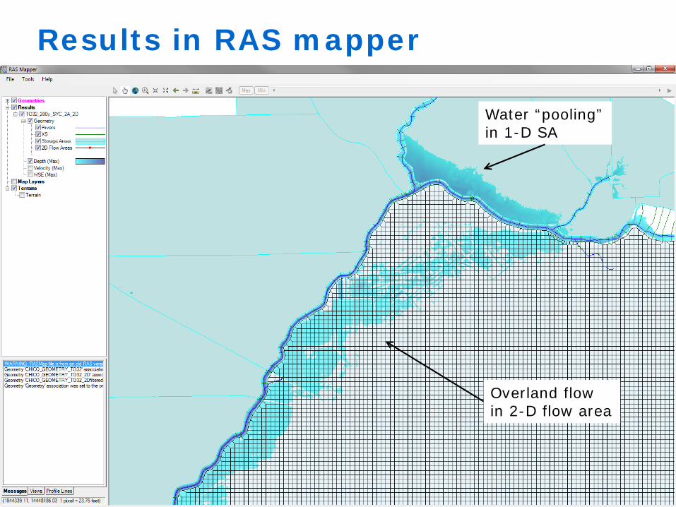
Results in RAS mapper

6

Water “pooling”in 1-D SA

Overland flowin 2-D flow area

“Full” 2-D depth-averaged (Saint Venant or shallow water) equations

• To make pretty 2-D pictures you need to solve these equations.

7

𝜕𝜕 ℎ𝑈𝑈𝜕𝜕𝑡𝑡

+𝜕𝜕𝜕𝜕𝑥𝑥

ℎ𝑈𝑈2 +𝑔𝑔ℎ2

2+𝜕𝜕𝜕𝜕𝑦𝑦

ℎ𝑈𝑈𝑈𝑈 = −𝑔𝑔ℎ 𝑆𝑆𝑜𝑜𝑜𝑜 + 𝑆𝑆𝑓𝑓𝑜𝑜 +𝜕𝜕 𝑇𝑇𝑜𝑜𝑜𝑜𝜕𝜕𝑥𝑥

+𝜕𝜕 𝑇𝑇𝑜𝑜𝑥𝑥𝜕𝜕𝑦𝑦

𝜕𝜕ℎ𝜕𝜕𝑡𝑡

+𝜕𝜕 ℎ𝑈𝑈𝜕𝜕𝑥𝑥

+𝜕𝜕 ℎ𝑈𝑈𝜕𝜕𝑦𝑦

= 0

𝜕𝜕 ℎ𝑈𝑈𝜕𝜕𝑡𝑡

+𝜕𝜕𝜕𝜕𝑥𝑥

ℎ𝑈𝑈𝑈𝑈 +𝜕𝜕𝜕𝜕𝑦𝑦

ℎ𝑈𝑈2 +𝑔𝑔ℎ2

2= −𝑔𝑔ℎ 𝑆𝑆𝑜𝑜𝑥𝑥 + 𝑆𝑆𝑓𝑓𝑥𝑥 +

𝜕𝜕 𝑇𝑇𝑜𝑜𝑥𝑥𝜕𝜕𝑥𝑥

+𝜕𝜕 𝑇𝑇𝑥𝑥𝑥𝑥𝜕𝜕𝑦𝑦

𝑆𝑆𝑓𝑓𝑜𝑜 =𝑛𝑛𝑈𝑈 𝑈𝑈2 + 𝑈𝑈2

𝐶𝐶2 ℎ ⁄4 3 𝑆𝑆𝑓𝑓𝑥𝑥 =𝑛𝑛𝑈𝑈 𝑈𝑈2 + 𝑈𝑈2

𝐶𝐶2 ℎ ⁄4 3

𝑇𝑇𝑜𝑜𝑜𝑜 = 2𝜈𝜈𝑡𝑡𝜕𝜕 ℎ𝑈𝑈𝜕𝜕𝑥𝑥 𝑇𝑇𝑜𝑜𝑥𝑥 = 𝜈𝜈𝑡𝑡

𝜕𝜕 ℎ𝑈𝑈𝜕𝜕𝑥𝑥

+𝜕𝜕 ℎ𝑈𝑈𝜕𝜕𝑦𝑦

𝑇𝑇𝑜𝑜𝑜𝑜 = 2𝜈𝜈𝑡𝑡𝜕𝜕 ℎ𝑈𝑈𝜕𝜕𝑦𝑦

where,

𝑆𝑆𝑜𝑜𝑜𝑜 =𝜕𝜕𝑧𝑧𝑏𝑏𝜕𝜕𝑥𝑥

𝑆𝑆𝑜𝑜𝑥𝑥 =𝜕𝜕𝑧𝑧𝑏𝑏𝜕𝜕𝑦𝑦

“Approximate” 2-D depth-averaged (diffusive wave) equations

• Neglect convective acceleration terms.

8

𝜕𝜕 ℎ𝑈𝑈𝜕𝜕𝑡𝑡

+𝜕𝜕𝜕𝜕𝑥𝑥

ℎ𝑈𝑈2 +𝑔𝑔ℎ2

2+𝜕𝜕𝜕𝜕𝑦𝑦

ℎ𝑈𝑈𝑈𝑈 = −𝑔𝑔ℎ 𝑆𝑆𝑜𝑜𝑜𝑜 + 𝑆𝑆𝑓𝑓𝑜𝑜 +𝜕𝜕 𝑇𝑇𝑜𝑜𝑜𝑜𝜕𝜕𝑥𝑥

+𝜕𝜕 𝑇𝑇𝑜𝑜𝑥𝑥𝜕𝜕𝑦𝑦

𝜕𝜕ℎ𝜕𝜕𝑡𝑡

+𝜕𝜕 ℎ𝑈𝑈𝜕𝜕𝑥𝑥

+𝜕𝜕 ℎ𝑈𝑈𝜕𝜕𝑦𝑦

= 0

𝜕𝜕 ℎ𝑈𝑈𝜕𝜕𝑡𝑡

+𝜕𝜕𝜕𝜕𝑥𝑥

ℎ𝑈𝑈𝑈𝑈 +𝜕𝜕𝜕𝜕𝑦𝑦

ℎ𝑈𝑈2 +𝑔𝑔ℎ2

2= −𝑔𝑔ℎ 𝑆𝑆𝑜𝑜𝑥𝑥 + 𝑆𝑆𝑓𝑓𝑥𝑥 +

𝜕𝜕 𝑇𝑇𝑜𝑜𝑥𝑥𝜕𝜕𝑥𝑥

+𝜕𝜕 𝑇𝑇𝑥𝑥𝑥𝑥𝜕𝜕𝑦𝑦

𝑆𝑆𝑓𝑓𝑜𝑜 =𝑛𝑛𝑈𝑈 𝑈𝑈2 + 𝑈𝑈2

𝐶𝐶2 ℎ ⁄4 3 𝑆𝑆𝑓𝑓𝑥𝑥 =𝑛𝑛𝑈𝑈 𝑈𝑈2 + 𝑈𝑈2

𝐶𝐶2 ℎ ⁄4 3

𝑇𝑇𝑜𝑜𝑜𝑜 = 2𝜈𝜈𝑡𝑡𝜕𝜕 ℎ𝑈𝑈𝜕𝜕𝑥𝑥 𝑇𝑇𝑜𝑜𝑥𝑥 = 𝜈𝜈𝑡𝑡

𝜕𝜕 ℎ𝑈𝑈𝜕𝜕𝑥𝑥

+𝜕𝜕 ℎ𝑈𝑈𝜕𝜕𝑦𝑦

𝑇𝑇𝑜𝑜𝑜𝑜 = 2𝜈𝜈𝑡𝑡𝜕𝜕 ℎ𝑈𝑈𝜕𝜕𝑦𝑦

where,

𝑆𝑆𝑜𝑜𝑜𝑜 =𝜕𝜕𝑧𝑧𝑏𝑏𝜕𝜕𝑥𝑥

𝑆𝑆𝑜𝑜𝑥𝑥 =𝜕𝜕𝑧𝑧𝑏𝑏𝜕𝜕𝑦𝑦

0

00

0

Flow in a spillway chute

Supercritical flow with a hydraulic jump

Project background

• PMF study• Spillway capacity study

• Original study used HEC-RAS 1-D• Inundation and erosion potential study

• Used HEC-RAS 2-D• Extended 2-D model into spillway chute to provide proper

inflow conditions to the floodplain• Updated original 1-D spillway study with 2-D spillway

results near the hydraulic jump• 2-D analysis includes supercritical flow in spillway chute,

and hydraulic jump in stilling basin

10

Terrain

11Spillway

Stillingbasin

Model domain

12

Inflowhydrograph

1-D SAs

2-D flow area

jump

Updated2-D mesh

Updated2-D mesh

Manual spillway mesh refinement

13

Original2-D mesh HEC-RAS geometry file

Storage Area Is2D=-1Storage Area Point Generation Data=0,0,10,10Storage Area 2D Points= 18960X-coord Y-coord X-coord Y-coordX-coord Y-coord X-coord Y-coordX-coord Y-coord X-coord Y-coordX-coord Y-coord X-coord Y-coord......................

Inundation results (maximum depth)

14

deeper

jump

Inflowhydrograph

Inundation results (maximum velocity)

15

faster

jump

Inflowhydrograph

Spillway characteristics

16

• Width: B≈20 ft• Slope: So≈0.27, θ≈15°• Q≈7,247 cfs (Vmax≈60 fps)• Fmax≈4.5

So

1θ

• HEC-RAS:• Jump height: d2/d1 ≈ 3.4 • Jump length: 125ft < L < 150ft

Spillway WSP results

17

HEC-RAS 2-DHEC-RAS 1-D

d1≈5.5ftV1≈60fpsF1≈4.5

d2≈18.6ftV2≈9.3fpsF2≈0.38

L

• Jump height:• HEC-RAS: d2/d1 ≈ 3.4 • USBR: d2/d1 ≈ 5.7

• Jump length:• HEC-RAS: L ≈ 135ft• USBR: L ≈ 190ft

• USBR results represent upper limit because some flow “leaks” over our spillway walls and the spillway becomes slightly wider

Spillway hydraulic jump (comparison with USBR measurements)

18

from USBR EM 25 (1984) “Hydraulic design of stilling basins and energy dissipators”

Spillway 2-D model summary

• 2-D mesh was manually refined in the spillway• Modeled supercritical flow in the spillway• Hydraulic jump was modeled “internally” (without

boundary condition influence)• Flow entering the floodplain was modeled “internally”

(with “proper” model computed velocity and depth)• High speed spillway flow:

• Required using full momentum equations• Required a small time step for stability purposes• Resulted in longer model run times

19

Flow around a 180° channel bend

Subcritical flow with superelevation and velocity redistribution

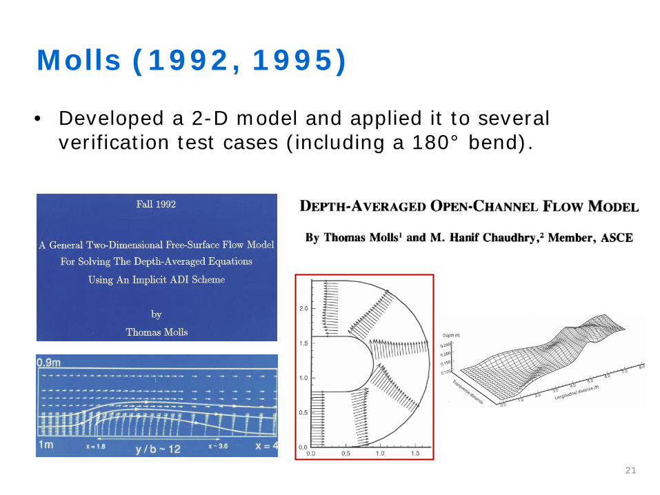
• Developed a 2-D model and applied it to several verification test cases (including a 180° bend).

Molls (1992, 1995)

21

Bend characteristics

• 180° bend with rectangular (B=0.8 m) cross section and straight upstream and downstream reaches

• Horizontal bottom (S0=0)• “Tight” bend, mean radius-to-width ratio of 1.0• Smooth channel, n = 0.01• Subcritical flow, Q = 0.0123 m3/s and F = 0.11• No flow separation at bend exit• Experimental data collected by Rozovskii (1957) and

reported in Leschziner and Rodi (1978) and Molls and Chaudhry (1995)

22

Bend data

23

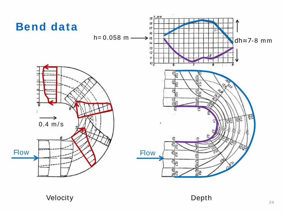
Bend data

24Velocity Depth

Flow Flow

0.4 m/s

h=0.058 m dh≈7-8 mm

Spiral flow in a bend (not captured by 2-D equations)

25from Blanckaert and de Vriend (2004)

r

z

θ

vr

vz

vθ

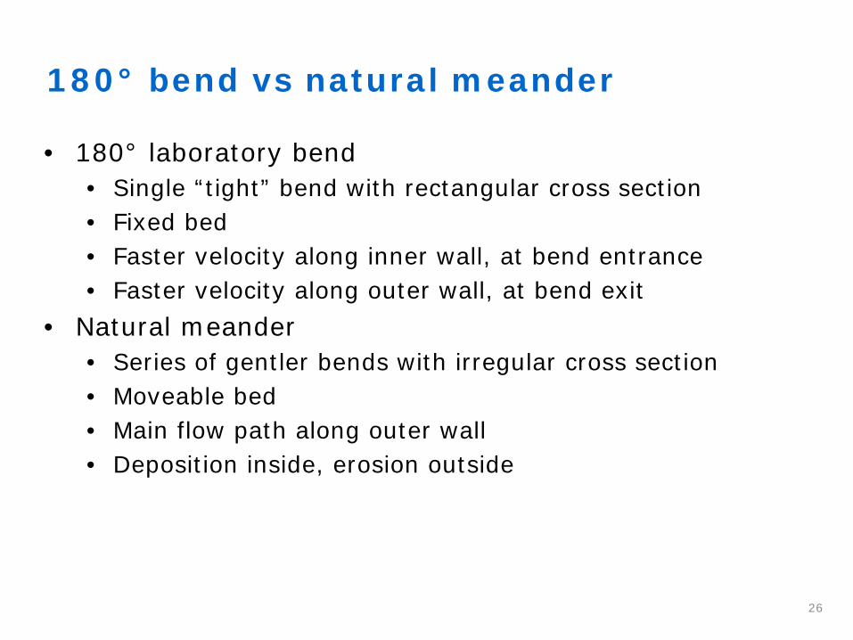
180° bend vs natural meander

• 180° laboratory bend• Single “tight” bend with rectangular cross section• Fixed bed• Faster velocity along inner wall, at bend entrance• Faster velocity along outer wall, at bend exit

• Natural meander• Series of gentler bends with irregular cross section• Moveable bed• Main flow path along outer wall• Deposition inside, erosion outside

26

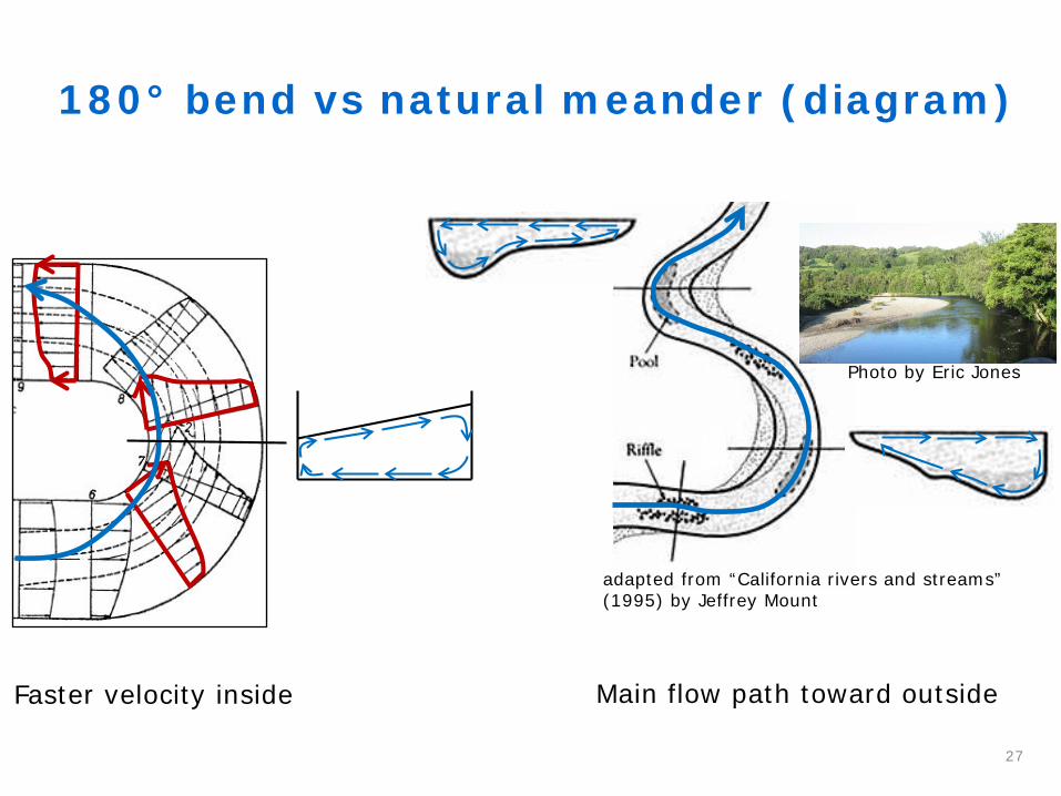
180° bend vs natural meander (diagram)

27

Faster velocity inside Main flow path toward outside

adapted from “California rivers and streams” (1995) by Jeffrey Mount

Photo by Eric Jones

Bend HEC-RAS initial setup

• HEC-RAS results show “proper” trends

28

Vmag (m/s)

Q=0.0123 m3/s

h≈0.

057

m

B=0.8 m

Rc=0.8 m

dx=dy=0.04 m

2 grids with similar grid cell size but different orientation

29HEC-RAS generated grid(initial setup)

Curvilinear grid (manually created)

Effect of grid orientation

30HEC-RAS generated grid(initial setup)

Curvilinear grid (manually created)More closely matches experimental data,but bend inner wall velocity is too low

Vmag (m/s)

V≈0.34 m/s

V≈0.19 m/s

V≈0.33 m/s

V≈0.12 m/s

Bend HEC-RAS final setup(yields “best”results)

• “Full” momentum equations• Curvilinear grid with dx = 0.02 m (reduced from 0.04)• dt = 0.05 s (Cr ≈ 1)• Other default parameters (no eddy viscosity)

31

Vmag (m/s)

Q=0.0123 m3/s

h≈0.

057

m

Bend HEC-RAS final velocity results

32

Vmag (m/s)

Q=0.0123 m3/sU0=0.265 m/s B

A

A

B

DC

C

D

E

F

E

F

Note: Ut/U0=1.5 Ut=0.4m/s

HEC-RAS 2-D

Bend HEC-RAS final depth results

33

Depth (cm)

5.0

6.2

B

A

C

E

D

F

B

A

C

ED

F

HEC-RAS 2-D (inner)HEC-RAS 2-D (outer)

Courant Number (Cr)

• Numerical stability criterion that imposes a constraint on the time step (dt), the grid cell size (dx), and the flow velocity (V)

• Cr = V∙(dt/dx)• Rearranging provides a way to estimate the

computational time step:• dt = Cr∙(dx/V)• Typical Cr range: 0.5 < Cr < 5• A rule of thumb is to start with Cr≈1

• For final setup: dt ≈ 1∙(0.02/0.4) = 0.05 s

34

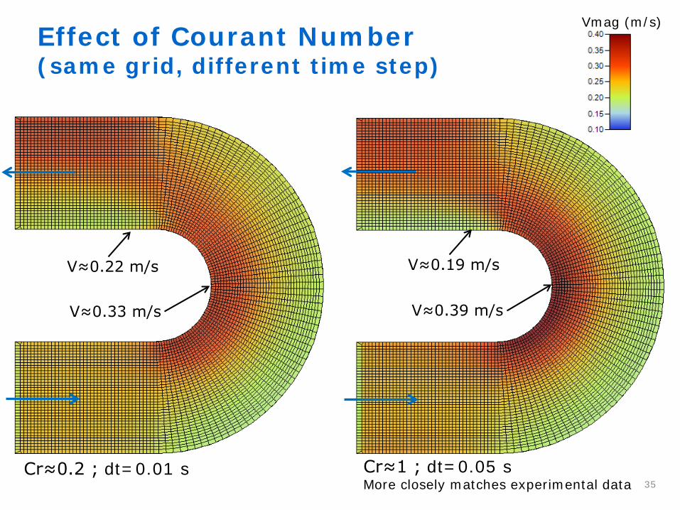
Effect of Courant Number(same grid, different time step)

35Cr≈0.2 ; dt=0.01 s Cr≈1 ; dt=0.05 s

More closely matches experimental data

Vmag (m/s)

V≈0.39 m/s

V≈0.19 m/s

V≈0.33 m/s

V≈0.22 m/s

Bend HEC-RAS Courant sensitivity velocity results

36

Vmag (m/s)

Q=0.0123 m3/sU0=0.265 m/s B

A

A

B

DC

C

D

E

F

E

F

Note: Ut/U0=1.5 Ut=0.4m/s

Cr≈1.0 ; dt=0.05sCr≈0.2 ; dt=0.01s

HEC-RAS 2-D

Bend HEC-RAS Courant sensitivity depth results

37

Depth (cm)

5.0

6.2

B

A

C

E

D

F

B

A

C

ED

F

Inner (Cr≈1.0 ; dt=0.05s)Inner (Cr≈0.2 ; dt=0.01s)

HEC-RAS 2-D

Outer (Cr≈1.0 ; dt=0.05s)Outer (Cr≈0.2 ; dt=0.01s)

180° bend 2-D model summary

• Use “full” momentum equations

• HEC-RAS results:• Reproduce properly the bend flow characteristics

(superelevation and velocity redistribution)• Are consistent with previous 2-D results and match well

with the experimental data• Are influenced by grid cell size and orientation• Are influenced by the computational time step

• 2-D studies should include grid cell size and time step sensitivity test

38

2-D modeling is a new feature in HEC-RAS v5.0

but it’s been around for quite a while

Kuipers and Vreugdenhil (1973)

40

Questions?

• Tom Molls:• tmolls@ford-consulting.com

• Presentation and data available at:• www.ford-consulting.com\highlights

• HydroCalc:• www.hydrocalc2000.com

41

Backup slides

42

• Approximate bend flow as irrotational vortex• Assume: vr=0 ; vz=0 ; dvθ/dz=0 ; dp/dθ=0 ; d/dt=0• (1/ρ)∙∂p/∂r = v2

θ/r• Assume: p=ρgh ; vθ=V=Q/A ; r = Rc

• (ρ/ρ)g∙∂h/∂r = V2/Rc

�hi

ho∂h=

V2

gRc�ri

rodr

ho−hi =V2

gRcro−ri

dh=V2BgRc

Superelevation (design manual equation)

43

r

zθ

vr=0

vz=0

vθ

dh

• B=0.8 m• Rc=0.8 m• Q = 0.0123 m3/s• hin ≈ 5.8 cm • Vin = Q/Ain = 0.265 m/s

dh=V2BgRc

=0.2652�0.89.81∙0.8 =0.0072 m

Superelevation (design calculation estimate)

44

dh≈7-8 mm

Corps EM1110-2-1601 Hydraulic Design of Flood Control Channels