HEAT TRANSFER IN A ROUND CC MOULD: MEASUREMENT, MODELLING AND VALIDATION

W. Rauter, M. Erker, W. Brandl – voestalpine Stahl Donawitz GmbH & Co KG, Leoben, Austria

S. Michelic, C. Bernhard – Christian Doppler Laboratory for Metallurgical Fundamentals of Continuous Casting Processes, Chair of Metallurgy, University of Leoben, Austria

ABSTRACT The heat removal in the continuous casting mould is a decisive factor for product quality and process safety. This quantity is affected by different process parameters, most noticeably by the steel composition, the casting velocity, the mould powder and the mould taper. Although the total heat transfer between strand and mould is easily determined through the temperature increase between primary water inlet and outlet, it only allows general conclusions on the conditions inside the mould. However, local changes in the heat transfer affect the uniformity of shell growth and in consequence the probability of surface and subsurface defect formation. The determination of the local heat transfer is rather complex, demanding the instrumentation of a mould with numerous thermocouples and subsequent inverse modelling. The present paper deals with the results of such heat transfer measurements in a 230 mm round mould at the CC3 of voestalpine Stahl Donawitz for a wide variety of steel grades under different process conditions. Additionally the paper illustrates results of a heat transfer model and contrasts them to the practical measurements. The satisfying correspondence between measured and calculated results points to the correctness of the assump-tions and boundary conditions. KEYWORDS heat transfer; mould instrumentation; plant trials; inverse modelling; heat transfer modelling INTRODUCTION voestalpine Stahl Donawitz GmbH & Co KG is part of the Division Railway Systems of voestalpine AG. It supplies the Railway Systems rolling mills with high quality billets and blooms for the production of railways, wires and seamless tubes. In addition – as shown in Fig. 1 – external customers besides voestalpine AG are also supplied with semi finished-products. The present work deals with the mould heat transfer of the five strand bloom caster CC3, which was commissioned in May 2000. The main machine data are listed in Tab. 1. The production spectrum of voestalpine Stahl Donawitz GmbH & Co KG covers a wide range of different steel grades, starting from low carbon steels for drawing grades up to high carbon steels for roller bearing steel. Due to the considerable differences in carbon contents, the mould heat transfer, which is one of the most important quantities in continuous casting, since it substantially influences the product quality, is highly influenced. Next to the steel composition, other process parameters like casting speed, mould taper and mould powder are also major issues which influence the heat transfer. Basically the heat transfer is determined by the temperature increase of the mould cooling water between inlet and outlet. Thereby, a general view on the heat transfer conditions can be gained. Owing to the fact that local changes in heat transfer can influence the uniformity of the steel shell, e. g. due to gap formation, the local heat transfer is of increasing importance for the reasons mentioned above. Therefore, extensive plant trials with an instrumented mould were conducted in order to record the temperature profiles during casting. Thereafter, an inverse model is used to calculate the heat withdrawal from the mould on the basis of the recorded temperatures.

Additionally, a heat transfer model which allows an estimation of the heat flux as a function of steel composition and casting parameters is presented and its results are compared to those from the inverse model.

Fig.1: Flowchart of voestalpine Stahl Donawitz GmbH und Co KG – Business Year 06/07.

Main Machine Data Start Up Year 2000 Capacity 1.2 Mta-1 Heat Size 67 t Number of strands 5 Radius 12 m Metallurgical length (max) 35.5 m Mould length 0.8 m Mould type Tube Bloom section 230 mm round 283x390 optional Casting Speed 1.2 – 1.75 mmin-1 Tundish capacity 29 t EMS Mould stirrer and moveable final stirrer Secondary cooling 5 zones air/mist

Tab. 1: Bloom caster CC3 main data.

1. HEAT TRANSFER MEASUREMENT AND MOULD INSTRUMENTATION As it has been mentioned above, two different ways of quantifying the heat transfer in the mould exist. On the one hand, the so-called integral heat flux as an overall quantity for the extracted amount of heat, and on the other hand the local heat flux. Generally, the integral heat flux is given by

m

OHpOH

ATcm

QΔ⋅⋅

= 22 ,&& (1)

where Q& is the integral heat flux in MWm-2, OHm

2& the water flow rate in kgs-1, OHpc

2, the heat capacity of water in Jkg-1K-1, TΔ the temperature increase of the cooling water in K and mA the active mould area in m2. The inlet cooling water temperature is measured with a Pt100 sensor for all the five strands, while the outlet cooling water temperature is measured separately for each strand, also with a Pt100 sensor. The cooling water flow is detected with an inductive flow meter, which is applied next to the cooling water outlet. All relevant values are stored into a database at a fixed time interval of 10 s. On the other hand, the determination of the local heat flux is much more complex. In order to get an overview of local changes in heat flux, many thermocouples in different regions in the mould have to be installed. For the present work, the mould was instrumented with 26 thermocouples – 4 around the circumference of the mould in 7 different planes from the top to the bottom, as illustrated in Fig. 2a. Generally, the meniscus region was equipped more densely than lower regions near to the outlet of the mould, because this region is essential for the characterisation of a representative axial heat transfer. One thermocouple was placed above the meniscus, to cover the whole mould length as good as possible. The mould was made of ELBRODUR, a copper alloy with Cr and Zr, with a thickness of 20 mm and had a constant linear taper of 1.45 %m-1. In order to prevent the copper mould from excessive abrasion, a 100 µm thick wear layer made of hard chromium, was applied at the hot face. The total mould length was 800 mm, the typical active length was 750 mm. The mould cooling water rate ranges between 1750 lmin-1 to 2000 lmin-1 depending on the steel quality.

Fig.2: Mould instrumentation: a) Position of thermocouples in the mould and b) Schematic mould

wall temperature setup.

Data acquisition

unit

R

2 mm

20 mm

Hot Face Cold Face

Data

Type K

a) b)

Type K thermocouples were employed for measuring the mould wall temperatures. In order to get lowest response times, the thermocouples were fixed two millimetres behind the hot face as shown in Fig. 2b. For keeping the mould stirrer influence as low as possible, two measures were taken: Firstly, the compensating lines were twisted thus keeping the disturbances induced by the magnetic field as low as possible. Secondly, a real low pass filter was used right before the acquisition unit. The monitoring frequency was 20 Hz. Hence, the recorded values were time-averaged with a data acquisition unit linked to a commercial PC. 2. MOULD TEMPERATURE MEASUREMENTS The conducted measurements encompass a wide variety of steel compositions and casting parameters. The compositions and casting conditions of all steels discussed in this publication are listed in Tab. 2. Additionally, the types of mould powders used during casting are listed since the choice of mould powder substantially influences the resulting heat flux.

Casting Series

Steel Grade wt.-%C wt.-%Si wt.-%Mn wt.-%Ni wt.-%Cr vc, mmin-1

Mould Powder Type

CS1 A 0.07 0.20 0.67 0.02 0.03 1.65 MP1 CS2 B 0.18 0.26 1.54 0.03 0.05 1.25 MP2 CS3 C 0.20 0.28 1.29 0.02 0.04 1.25 MP2 CS4 D 0.18 0.25 1.00 0.02 0.04 1.45 MP2 CS5 D 0.18 0.25 1.00 0.02 0.04 1.55 MP2 CS6 E 0.27 0.31 0.80 0.03 1.35 1.60 MP2 CS7 F 0.38 0.04 0.74 0.02 0.17 1.60 MP2 CS8 G 0.42 0.26 0.81 0.03 0.97 1.60 MP2 CS9 H 0.73 0.23 0.50 0.01 0.02 1.40 MP3

CS10 I 0.80 0.26 0.74 0.03 0.30 1.45 MP3 CS11 J 1.02 0.32 0.30 0.03 1.50 1.20 MP3

Tab. 2: Composition of investigated steel grades in wt.-%, casting speeds and mould powder.

A typical mould wall temperature response from two different thermocouples is shown in Fig. 3. The temperature response from the thermocouple which is near the meniscus region (80 mm from the top of the mould) is strongly fluctuating. In contrast, the temperatures from the lower part of the mould, e.g. at 730 mm, are more uniform. This behaviour is common for nearly all investigated steel grades. The considerable differences in temperature fluctuation between the meniscus region and areas below result from the uneven slag rim thickness and the mould powder consumption, which may possibly be caused by the manual mould powder feeding. This leads to both, uneven shell growth and gap formation between mould and strand, thus causing a stronger fluctuation of the temperatures. In the lower regions of the mould, these fluctuations strongly diminish due to the fact that the strand shell is thicker, thus increasing the heat resistance which has a stabilising effect on the heat transfer. Moreover, the following differences between the investigated steel grades can be observed: The comparison of Fig. 4a and Fig. 4b shows that the time averaged temperature responses from the meniscus region are between 185°C and 240 °C. These differences are due to differences in casting speed, mould powder type and steel composition. The temperature maximum is roughly 30 mm below the meniscus which is in good correspondence to results of other studies [1,2]. Additionally,

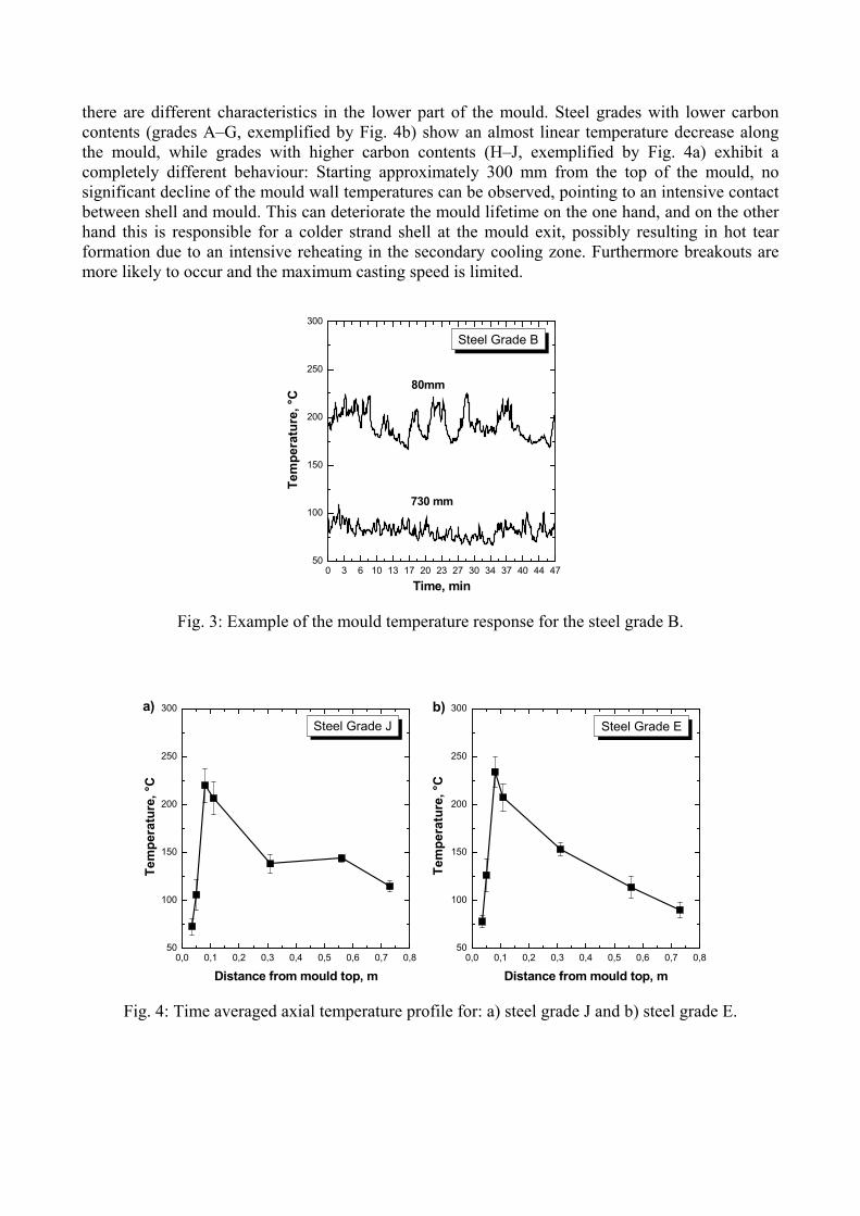
there are different characteristics in the lower part of the mould. Steel grades with lower carbon contents (grades A–G, exemplified by Fig. 4b) show an almost linear temperature decrease along the mould, while grades with higher carbon contents (H–J, exemplified by Fig. 4a) exhibit a completely different behaviour: Starting approximately 300 mm from the top of the mould, no significant decline of the mould wall temperatures can be observed, pointing to an intensive contact between shell and mould. This can deteriorate the mould lifetime on the one hand, and on the other hand this is responsible for a colder strand shell at the mould exit, possibly resulting in hot tear formation due to an intensive reheating in the secondary cooling zone. Furthermore breakouts are more likely to occur and the maximum casting speed is limited.

0 3 6 10 13 17 20 23 27 30 34 37 40 44 4750

100

150

200

250

300

Steel Grade B

730 mm

Te

mpe

ratu

re, °

C

Time, min

80mm

Fig. 3: Example of the mould temperature response for the steel grade B.

0,0 0,1 0,2 0,3 0,4 0,5 0,6 0,7 0,850

100

150

200

250

300

Tem

pera

ture

, °C

Distance from mould top, m

a)Steel Grade J

0,0 0,1 0,2 0,3 0,4 0,5 0,6 0,7 0,850

100

150

200

250

300

Steel Grade Eb)

Tem

pera

ture

, °C

Distance from mould top, m

Fig. 4: Time averaged axial temperature profile for: a) steel grade J and b) steel grade E.

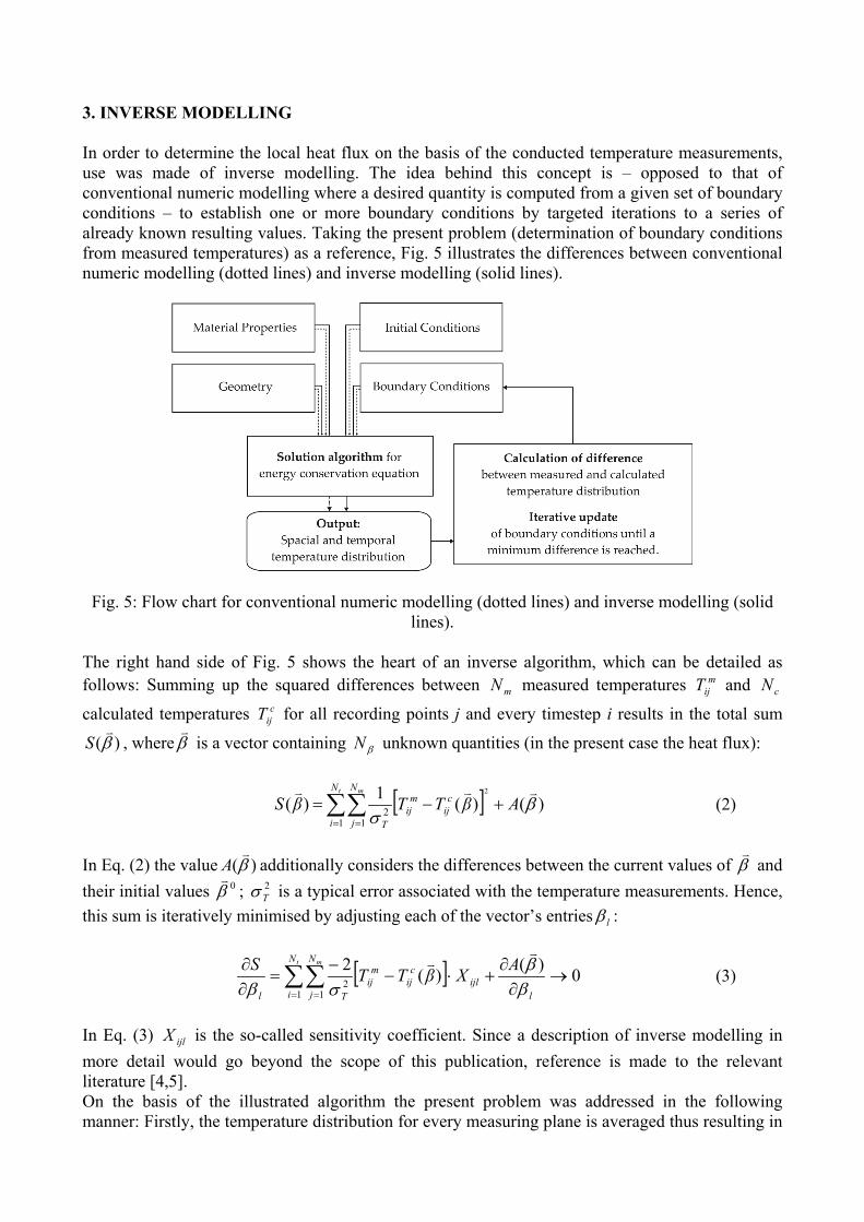
3. INVERSE MODELLING In order to determine the local heat flux on the basis of the conducted temperature measurements, use was made of inverse modelling. The idea behind this concept is – opposed to that of conventional numeric modelling where a desired quantity is computed from a given set of boundary conditions – to establish one or more boundary conditions by targeted iterations to a series of already known resulting values. Taking the present problem (determination of boundary conditions from measured temperatures) as a reference, Fig. 5 illustrates the differences between conventional numeric modelling (dotted lines) and inverse modelling (solid lines).

Fig. 5: Flow chart for conventional numeric modelling (dotted lines) and inverse modelling (solid lines).

The right hand side of Fig. 5 shows the heart of an inverse algorithm, which can be detailed as follows: Summing up the squared differences between mN measured temperatures m

ijT and cN

calculated temperatures cijT for all recording points j and every timestep i results in the total sum

)(βv

S , where βv

is a vector containing βN unknown quantities (in the present case the heat flux):

[ ] )()(1)(1 1

2

2

βσ

vvvAβTTβS

t mN

i

N

j

cij

mij

T

+−=∑∑= =

(2)

In Eq. (2) the value )(β

vA additionally considers the differences between the current values of β

v and

their initial values 0βv

; 2Tσ is a typical error associated with the temperature measurements. Hence,

this sum is iteratively minimised by adjusting each of the vector’s entries lβ :

[ ] 0)()(21 1

2 →∂∂

+⋅−−

=∂∂ ∑∑

= = l

N

i

N

jijl

cij

mij

Tl

AXβTTS t m

ββ

σβ

vv

(3)

In Eq. (3) ijlX is the so-called sensitivity coefficient. Since a description of inverse modelling in more detail would go beyond the scope of this publication, reference is made to the relevant literature [4,5]. On the basis of the illustrated algorithm the present problem was addressed in the following manner: Firstly, the temperature distribution for every measuring plane is averaged thus resulting in

a uniform temperature distribution around the circumference of the mould. Admittedly this is not the case in casting practise due to local fluctuations which may result from mould powder inhomogeneities, shell deformation or other phenomena. Nonetheless on the whole, the error resulting from smoothing the temperatures is comparatively small, since the measuring time in the steady state casting period was long enough to ensure that local disturbances in the heat flux play a minor role. Consequently, it is possible to reduce the initially three-dimensional problem to a two-dimensional one, thus treating only a longitudinal slice of the total bloom. It has been mentioned that the present study only includes the treatment of steady states in the overall casting process, wherefore a constant heat flux distribution can be assumed over this casting period. The subsequent inverse modelling was carried out using the software tool CALCOSOFT-2D which uses the finite element method for solving the following equation,

),,()div()()( zrTqTt

THT&+⋅=

∂∂ gradκρ (4)

which is a derivation of the law of energy conservation coupled with Fourier’s law of heat conduction. In Eq. (3) )(Tρ denotes the temperature-dependent density in kgm-3, )(TH the enthalpy in Jkg-1, t the time in s, )(Tκ the thermal conductivity in Wm-1K-1, T the temperature in K, r and z are coordinates in m; q& is a source term accounting for the latent heat release or the heat extracted from the system (water cooling in the mould). The temperature-dependent material properties )(Tρ , )(TH and )(Tκ were calculated by the commercial software program IDS16[6]. 4. RESULTS Influence of steel composition and mould powder type In Fig. 6 the local heat flux calculated by the illustrated inverse model is depicted – the selection of casting series was done under the viewpoint of similar casting velocities; Fig. 6a shows the characteristics for the hypoperitectic steel grade A which is cast using mould powder type MP1; Fig. 6b several medium carbon steels (grades F and G) which are all cast with mould powder type MP2; Finally, Fig. 6c exemplifies the typical characteristics for high carbon steels (grades H and I). Additionally, the heat flux distribution is bounded by dotted grey lines which indicate the variability of the heat flux due to possible variations in the temperature measurements. Generally, all curves show a similar distribution of the local heat flux with an initial steep rise to a maximum slightly below the meniscus, followed by a decrease towards half mould length, and a further reduction of heat flux at the mould exit. The initial maximum is explained by the fact that the heat flux is enormous in absence of a solid steel shell. Exactly at the meniscus level, a solid slag rim which forms during casting has an isolating effect, wherefore the maximum heat flux can be observed slightly below. Once a solid shell has formed, the heat flux decreases substantially – a behaviour which is intensified by two additional factors: Firstly, the morphology of the mould powder changes due to falling temperature, thus increasing the percentage of solid powder, hence enhancing the systems isolation. Secondly, the solidification-caused contraction of the steel – potentially intensified by the δ/γ-transition – may cause a disproportionate diametrical decrease of the strand radius, thus resulting in the formation of a gap between the two interfaces. The atmosphere of the gap is currently under research, since gaseous components evaporating from the mould powder can cause changes. Whatsoever the composition of the gap may be, it is definitely causing a substantial decrease of the heat flux due to the considerably lower thermal conductivity of gases. In order to compensate for the shell shrinkage, the mould is tapered which will cause the shell to be pressed to the interface again in the lower section of the mould thus increasing the heat flux.

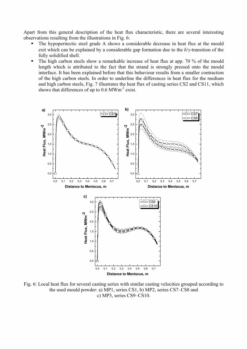
Apart from this general description of the heat flux characteristic, there are several interesting observations resulting from the illustrations in Fig. 6: The hypoperitectic steel grade A shows a considerable decrease in heat flux at the mould

exit which can be explained by a considerable gap formation due to the δ/γ-transition of the fully solidified shell.

The high carbon steels show a remarkable increase of heat flux at app. 70 % of the mould length which is attributed to the fact that the strand is strongly pressed onto the mould interface. It has been explained before that this behaviour results from a smaller contraction of the high carbon steels. In order to underline the differences in heat flux for the medium and high carbon steels, Fig. 7 illustrates the heat flux of casting series CS2 and CS11, which shows that differences of up to 0.6 MWm-2 exist.

0,0 0,1 0,2 0,3 0,4 0,5 0,6 0,7

0,0

0,5

1,0

1,5

2,0

2,5

3,0

CS1

Hea

t Flu

x, M

Wm

-2

Distance to Meniscus, m

a)

0,0 0,1 0,2 0,3 0,4 0,5 0,6 0,7

0,0

0,5

1,0

1,5

2,0

2,5

3,0

CS7 CS8

Hea

t Flu

x, M

Wm

-2

Distance to Meniscus, m

b)

0,0 0,1 0,2 0,3 0,4 0,5 0,6 0,7

0,0

0,5

1,0

1,5

2,0

2,5

3,0

Hea

t Flu

x, M

Wm

-2

Distance to Meniscus, m

CS9 CS10

c)

Fig. 6: Local heat flux for several casting series with similar casting velocities grouped according to

the used mould powder: a) MP1, series CS1, b) MP2, series CS7–CS8 and c) MP3, series CS9–CS10.

0,0 0,1 0,2 0,3 0,4 0,5 0,6 0,7

0,0

0,5

1,0

1,5

2,0

2,5

3,0

CS2 CS11

Hea

t Flu

x, M

Wm

-2

Distance to Meniscus, m

Fig. 7: Heat flux for casting series CS2 and CS11 (equal casting velocities, different compositions). Influence of casting velocity It is generally accepted that a rise in casting velocity leads to an increased heat withdrawal in the mould. This is confirmed by the behaviour illustrated in Fig. 8 which shows the heat flux for steel grade D, once cast with 1.45 mmin-1 and once with 1.55 mmin-1. It can be seen that the general distribution of the heat flux remains very similar, the increased casting velocity leads to an overall increase of heat withdrawal which – in terms of integral heat flux – amounts to app. 0.1 MWm-2.

0,0 0,1 0,2 0,3 0,4 0,5 0,6 0,7

0,0

0,5

1,0

1,5

2,0

2,5

3,0

CS4 CS5

Hea

t Flu

x, M

Wm

-2

Distance to Meniscus, m

Fig. 8: Changes in heat flux for varying casting velocities for steel grade D: CS4: 1.45 mmin-1 and CS5: 1.55 mmin-1.

Comparison via the Integral Heat Flux In order to ascertain the results of the inverse model, the integral heat flux as a measure of the overall heat withdrawal, is compared for all steel grades. It has been illustrated that the deter-mination of the integral heat flux is carried out by measuring the temperature increase of the cooling water (see Eq. (1)). Additionally, integrating the local heat flux curve will also yield the total amount of heat extracted from the system, thus allowing a comparison of the two quantities. The result of this comparison, which incorporates all casting series CS1–CS11, is illustrated in Fig. 9. Taking into account that the temperature measurements for the local heat flux are afflicted with both, systematic and random errors, the grey area in the figure should imply a certain variability of

the single points. Since the satisfying correlation between the measured values and those from the inverse model, the soundness of this technique for determining the local heat flux is underlined.

Fig. 9: Comparison of integral heat flux determined by inverse modelling and by direct measurement at the plant – the grey area indicates a certain variability of the values.

5. HEAT TRANSFER MODELLING In order to minimise measurement expenditures in future, a model for describing the heat transfer in a round mould has been developed [7] on the basis of an approach by Han et al. [8]. Generally speaking, it is assumed that heat transfer mechanisms always act in parallel. Since the two decisive heat transfer mechanisms in the case of continuous casting are heat conduction and radiation, the model idea is built up appropriately: Fig. 10 illustrates that heat conduction is composed of the heat transfer resistances of the mould mouldR , the gap gapR , the flux fluxR and the strand strandR superimposed by a radiative heat transfer denoted radR .

Fig. 10: Illustration of the model idea for estimating the total heat transfer in the CC mould.

1,3 1,4 1,5 1,6 1,7 1,8

1,3

1,4

1,5

1,6

1,7

1,8

Inte

gral

Hea

t Flu

x

Inve

rse

Mod

ellin

g, M

Wm

-2

Integral Heat Flux

Plant Data, MWm-2

Thus, the total heat transfer coefficient Th can be expressed by:

radstrandfluxgapmouldT

RRRRRh 11

++++

= (6)

Hence, the local heat flux q& in the mould is a product of heat transfer coefficient and temperature difference: ( )mouldstrandT TThq −⋅=& (7) Although a detailed explanation of the model together with quantifications for the single heat transfer resistances can be found elsewhere [7], it should be stated that the heart of this model is the estimation of the gap size and the thickness of the mould powder layer as functions of steel composition and casting parameters. The extent of the gap is estimated by a mechanical analysis of the strand shell which incorporates solidification shrinkage on the one hand and metallostatic pressure on the other. Since the model additionally accounts for the mould taper, it is possible to estimate the gap formation over the whole mould length. In order to approximate the thickness of the mould powder layer, a mould powder consumption model has been developed [7] which yields the layer’s thickness as a function of casting parameters and powder composition. In the following, the local heat flux from selected casting series of the above measurements will be contrasted to those calculated by the illustrated heat transfer model. In Fig. 11a CS11 is compared to the heat flux estimations from the model. It can be seen that the values correspond very well: the initial peak value of the heat flux lies in the same order of magnitude and the trend of the heat flux towards the mould exit is also reflected very well. Additionally, the correspondence of integral heat flux is very satisfactory. In order to investigate the model behaviour for changing casting speeds, CS4 and CS5 were taken as reference; Fig. 11b illustrates that the tendency of increasing heat flux for higher casting speeds is additionally reproduced very well – next to the good overall agreement of the heat flux. Although there are slight deviations of the heat flux in the upper region of the mould, the basic equivalence is acceptable; moreover the integral heat flux again matches very well.

0,0 0,1 0,2 0,3 0,4 0,5 0,6 0,7

0,0

0,5

1,0

1,5

2,0

2,5

3,0

Steel Grade J

Hea

t Flu

x, M

Wm

-2

Distance to Meniscus, m

Heat Transfer Model CS11

a)

0,0 0,1 0,2 0,3 0,4 0,5 0,6 0,7

0,0

0,5

1,0

1,5

2,0

2,5

3,0

Hea

t Flu

x, M

Wm

-2

Distance to Meniscus, m

Heat Transfer Model: vc=1.45 mmin-1

vc=1.55 mmin-1

CS4 CS5

Steel Grade Db)

Fig. 11: Comparison of the local heat flux determined by inverse modelling and by the heat transfer

modelling: a) for different compositions and b) for different casting speeds.

6. CONCLUSION The heat transfer in the continuous casting mould is a decisive factor for product quality and process safety. Local changes in heat transfer affect the uniformity of shell growth and in consequence the probability of surface and subsurface defect formation. Therefore, an extensive measurement campaign was conducted at the continuous caster CC3 of voestalpine Stahl Donawitz. Based on these measurements it was possible to illustrate differences in local heat flux for varying steel compositions and casting speeds, calculated by an inverse model. Taking the integral heat flux as a validation quantity, the good agreement of the results could be demonstrated. Additionally the measurements were compared to a heat transfer model which was developed in order to minimise future measurement efforts. The satisfying correspondence points to the correctness of the assumptions and boundary conditions. In future, the validated model will provide flexible thermal boundary conditions for process models, thus substituting further extensive temperature measure-ments. 7. ACKNOWLEDGEMENTS The authors would like to thank Mr. Z. Babilli for accomplishing the inverse calculations. Additionally, the partial funding of this work by the Austrian Ministry for Economy and Labour in the frame of the Christian Doppler Laboratories is gratefully acknowledged. REFERENCES 1) B. Wang, B.N. Walker and I.V. Samarasekera, Can. Met. Quat. 39, (2000), p. 441. 2) R.B. Mahapatra, J.K. Brimacombe and I.V. Samarasekera, Met. Mat. Trans. B 22B, (1991), p. 875. 3) A. Howe, Segregation and phase distribution during solidification of carbon, alloy and stainless steels, EUR 13303, ECSC, Luxembourg (1991). 4) M. Rappaz, M. Bellet and M. Deville, Numerical Modeling in Materials Science and Engineering, Springer-Verlag, Berlin (2003). 5) J. Beck, Parameter Estimation in Engineering and Science, John Wiley & Sons Inc., New York (1977). 6) J. Miettinen, Met. Mat. Trans. A 23A, (1992), p. 1155. 7) S. Michelic, C. Bernhard and R. Pierer, Proc. of the SteelSim 2007, Graz/Seggau (2007), p. 209. 8) H. Han, J. Lee, T. Yeo, Y. Won, K. Kim, K. Oh and J. Yoon, ISIJ Intern. 39, (1999), p. 445.