![Numerical Simulation of Heat Transfer During the Solidification … · · 2006-01-03Numerical Simulation of Heat Transfer During the Solidification of … , []} → → → →](https://static.fdocuments.net/doc/165x107/5adeb26e7f8b9ad66b8bded9/numerical-simulation-of-heat-transfer-during-the-solidification-simulation-of.jpg)
Heat-Transfer and Solidification Model of...
21
Heat-Transfer and Solidification Model of Continuous Slab Casting: CON1D YA MENG and BRIAN G. THOMAS A simple, but comprehensive model of heat transfer and solidification of the continuous casting of steel slabs is described, including phenomena in the mold and spray regions. The model includes a one-dimensional (1-D) transient finite-difference calculation of heat conduction within the solidifying steel shell coupled with two-dimensional (2-D) steady-state heat conduction within the mold wall. The model features a detailed treatment of the interfacial gap between the shell and mold, including mass and momentum balances on the solid and liquid interfacial slag layers, and the effect of oscillation marks. The model predicts the shell thickness, temperature distributions in the mold and shell, thickness of the resolidified and liquid powder layers, heat-flux profiles down the wide and narrow faces, mold water temperature rise, ideal taper of the mold walls, and other related phenomena. The important effect of the nonuniform distribution of superheat is incorporated using the results from previous three- dimensional (3-D) turbulent fluid-flow calculations within the liquid pool. The FORTRAN program CONID has a user-friendly interface and executes in less than 1 minute on a personal computer. Calibration of the model with several different experimental measurements on operating slab casters is presented along with several example applications. In particular, the model demonstrates that the increase in heat flux throughout the mold at higher casting speeds is caused by two combined effects: a thinner interfacial gap near the top of the mold and a thinner shell toward the bottom. This modeling tool can be applied to a wide range of practical problems in continuous casters. I. INTRODUCTION HEAT transfer in the continuous slab-casting mold is governed by many complex phenomena. Figure 1 shows a schematic of some of these. Liquid metal flows into the mold cavity through a submerged entry nozzle and is directed by the angle and geometry of the nozzle ports. [1] The direction of the steel jet controls turbulent fluid flow in the liquid cavity, which affects delivery of superheat to the solid/liquid interface of the growing shell. The liquid steel solidifies against the four walls of the water-cooled copper mold, while it is continuously withdrawn downward at the casting speed. Mold powder added to the free surface of the liquid steel melts and flows between the steel shell and the mold wall to act as a lubricant, [2] so long as it remains liquid. The resolidified mold powder, or “slag,” adjacent to the mold wall cools and greatly increases in viscosity, thus acting like a solid. It is thicker near and just above the meniscus, where it is called the “slag rim.” The slag cools rapidly against the mold wall, forming a thin solid glassy layer, which can devitrify to form a crystalline layer if its residence time in the mold is very long. [3] This relatively solid slag layer often remains stuck to the mold wall, although it is sometimes dragged intermittently downward at an average speed less than the casting speed. [4] Depending on its cooling rate, this slag layer may have a structure that is glassy, crystalline, or a combination of both. [5] So long as the steel shell remains above its crystallization temperature, a liquid slag layer will move downward, causing slag to be consumed at a rate balanced by the replenishment of bags of solid powder to the top surface. Still more slag is captured by the oscillation marks and other imperfections of the shell surface and carried downward at the casting speed. These layers of mold slag comprise a large resistance to heat removal, although they provide uniformity relative to the alternative of an intermittent vapor gap found with oil cast- ing of billets. Heat conduction across the slag depends on the thickness and conductivity of its layers, which, in turn, depends on their velocity profile, crystallization temperature, [6] viscosity, and state (glassy, crystalline, or liquid). The latter can be determined by the time-temperature-transformation (TTT) diagram measured for the slag, knowing the local cooling rate. [7,8,9] Slag conductivity depends mainly on the crystallinity of the slag layer and on the internal evolution of its dissolved gas to form bubbles. Shrinkage of the steel shell away from the mold walls may generate contact resistances or air gaps, which act as a further resistance to heat flow, especially after the slag is completely solid and unable to flow into the gaps. The surface roughness depends on the tendency of the steel shell to “ripple” during solidification at the meniscus to form an uneven surface with deep oscillation marks. This depends on the oscillation practice, the slag-rim shape and properties, and the strength of the steel grade relative to the ferrostatic pressure, mold taper, and mold distortion. These interfacial resistances predominantly control the rate of heat flow in the process. Finally, the flow of cooling water through vertical slots in the copper mold withdraws the heat and controls the temperature of the copper mold walls. If the “cold face” of the mold walls becomes too hot, boiling may occur, which causes variability in heat extraction and accompanying defects. Impurities in the water sometimes form scale deposits METALLURGICAL AND MATERIALS TRANSACTIONS B VOLUME 34B, OCTOBER 2003—685 YA MENG, Graduate Student, Department of Materials Science and Engineering, and BRIAN G. THOMAS, Professor, Department of Mechan- ical and Industrial Engineering, are with the University of Illinois at Urbana–Champaign, Urbana, IL 61801. Contact e-mail: [email protected] Manuscript submitted August 27, 2002.
-
Upload
truongdung -
Category
Documents
-
view
226 -
download
0
Transcript of Heat-Transfer and Solidification Model of...
Heat-Transfer and Solidification Model of Continuous Slab Casting CON1D
YA MENG and BRIAN G THOMAS
A simple but comprehensive model of heat transfer and solidification of the continuous casting ofsteel slabs is described including phenomena in the mold and spray regions The model includes aone-dimensional (1-D) transient finite-difference calculation of heat conduction within the solidifyingsteel shell coupled with two-dimensional (2-D) steady-state heat conduction within the mold wallThe model features a detailed treatment of the interfacial gap between the shell and mold includingmass and momentum balances on the solid and liquid interfacial slag layers and the effect of oscillationmarks The model predicts the shell thickness temperature distributions in the mold and shell thicknessof the resolidified and liquid powder layers heat-flux profiles down the wide and narrow faces moldwater temperature rise ideal taper of the mold walls and other related phenomena The importanteffect of the nonuniform distribution of superheat is incorporated using the results from previous three-dimensional (3-D) turbulent fluid-flow calculations within the liquid pool The FORTRAN programCONID has a user-friendly interface and executes in less than 1 minute on a personal computerCalibration of the model with several different experimental measurements on operating slab castersis presented along with several example applications In particular the model demonstrates that theincrease in heat flux throughout the mold at higher casting speeds is caused by two combined effectsa thinner interfacial gap near the top of the mold and a thinner shell toward the bottom This modelingtool can be applied to a wide range of practical problems in continuous casters
I INTRODUCTION
HEAT transfer in the continuous slab-casting mold isgoverned by many complex phenomena Figure 1 shows aschematic of some of these Liquid metal flows into the moldcavity through a submerged entry nozzle and is directed bythe angle and geometry of the nozzle ports[1] The directionof the steel jet controls turbulent fluid flow in the liquidcavity which affects delivery of superheat to the solidliquidinterface of the growing shell The liquid steel solidifiesagainst the four walls of the water-cooled copper mold whileit is continuously withdrawn downward at the casting speed
Mold powder added to the free surface of the liquid steelmelts and flows between the steel shell and the moldwall to act as a lubricant[2] so long as it remains liquid Theresolidified mold powder or ldquoslagrdquo adjacent to the moldwall cools and greatly increases in viscosity thus acting likea solid It is thicker near and just above the meniscus whereit is called the ldquoslag rimrdquo The slag cools rapidly against themold wall forming a thin solid glassy layer which candevitrify to form a crystalline layer if its residence time inthe mold is very long[3] This relatively solid slag layer oftenremains stuck to the mold wall although it is sometimesdragged intermittently downward at an average speed lessthan the casting speed[4] Depending on its cooling ratethis slag layer may have a structure that is glassy crystallineor a combination of both[5] So long as the steel shell remainsabove its crystallization temperature a liquid slag layer will
move downward causing slag to be consumed at a ratebalanced by the replenishment of bags of solid powder tothe top surface Still more slag is captured by the oscillationmarks and other imperfections of the shell surface and carrieddownward at the casting speed
These layers of mold slag comprise a large resistanceto heat removal although they provide uniformity relative tothe alternative of an intermittent vapor gap found with oil cast-ing of billets Heat conduction across the slag depends on thethickness and conductivity of its layers which in turn dependson their velocity profile crystallization temperature[6] viscosityand state (glassy crystalline or liquid) The latter can bedetermined by the time-temperature-transformation (TTT)diagram measured for the slag knowing the local coolingrate[789] Slag conductivity depends mainly on the crystallinityof the slag layer and on the internal evolution of its dissolvedgas to form bubbles
Shrinkage of the steel shell away from the mold wallsmay generate contact resistances or air gaps which actas a further resistance to heat flow especially after the slagis completely solid and unable to flow into the gaps Thesurface roughness depends on the tendency of the steel shellto ldquoripplerdquo during solidification at the meniscus to form anuneven surface with deep oscillation marks This dependson the oscillation practice the slag-rim shape and propertiesand the strength of the steel grade relative to the ferrostaticpressure mold taper and mold distortion These interfacialresistances predominantly control the rate of heat flow inthe process
Finally the flow of cooling water through vertical slotsin the copper mold withdraws the heat and controls thetemperature of the copper mold walls If the ldquocold facerdquo ofthe mold walls becomes too hot boiling may occur whichcauses variability in heat extraction and accompanyingdefects Impurities in the water sometimes form scale deposits
METALLURGICAL AND MATERIALS TRANSACTIONS B VOLUME 34B OCTOBER 2003mdash685
YA MENG Graduate Student Department of Materials Science andEngineering and BRIAN G THOMAS Professor Department of Mechan-ical and Industrial Engineering are with the University of Illinois atUrbanandashChampaign Urbana IL 61801 Contact e-mail bgthomasuiucedu
Manuscript submitted August 27 2002
686mdashVOLUME 34B OCTOBER 2003 METALLURGICAL AND MATERIALS TRANSACTIONS B
on the mold cold face which can significantly increase themold temperature especially near the meniscus where themold is already hot After exiting the mold the steel shellmoves between successive sets of alternating support rollsand spray nozzles in the spray zones The accompanyingheat extraction causes surface-temperature variations whilethe shell continues to solidify
It is clear that many diverse phenomena simultaneouslycontrol the complex sequence of events which govern heattransfer in the continuous casting process The present workwas undertaken to develop a fast simple and flexible modelto investigate these heat-transfer phenomena In particularthe model features a detailed treatment of the interfacial gapin the mold which is the most important thermal resistanceThe model includes heat mass momentum and forcebalances on the slag layers in the interfacial gap
This model is part of a larger comprehensive system ofmodels of fluid flow heat transfer and mechanical behaviorwhich is being developed and applied to study the formationof defects in the continuous casting process These othermodels are used to incorporate the effects of mold distor-tion[10] the influence of fluid flow in the liquid pool onsolidification of the shell[11] and coupled thermal-stressanalysis of the shell to find the reduction of heat transferacross the interface due to air-gap formation[12]
This article first describes the formulation of this modelwhich has been implemented into a user-friendly FORTRANprogram CONID on personal computers and UNIX work-stations Then validation of the model with analyticalsolutions and calibration with example plant measurementsare presented Finally the effect of casting speed on moldheat transfer is investigated as one example of the manyapplications of this useful modeling tool
II PREVIOUS WORK
Many mathematical models have been developed of thecontinuous casting process which are partly summarized inprevious literature reviews[131415] Many continuous-casting
models are very sophisticated (even requiring supercomputersto run) so are infeasible for use in an operating environmentThe earliest solidification models used one-dimensional(1-D) finite-difference methods to calculate the temperaturefield and growth profile of the continuously cast steelshell[1617] Many industrial models followed[1819] Thesemodels first found application in the successful predictionof metallurgical length which is also easily done by solv-ing the following simple empirical relationship for dis-tance (z) with the shell thickness (S) set to half the sectionthickness
[1]
where K is found from evaluation of breakout shells andcomputations Such models found further application introubleshooting the location down the caster of hot-tearcracks initiating near the solidification front[20] and in theoptimization of cooling practice below the mold to avoidsubsurface longitudinal cracks due to surface reheating[21]
Since then many advanced models have been developedto simulate further phenomena such as thermal stress and crack-related defects[122223] or turbulent fluid flow[24ndash28] coupledtogether with solidification For example a two-dimensional(2-D) transient stepwise coupled elasto-viscoplastic finite-element model tracks the behavior of a transverse slice througha continuously cast rectangular strand as it moves down throughthe mold at casting speed[12] This model is suited for simulatinglongitudinal phenomena such as taper design[29] longitudinalcracks[30] and surface depressions[31] Other casters havebeen modeled using three-dimensional (3-D) coupled fluidflowndashsolidification models[27] based on control-volume or finite-difference approaches at the expense of greater computationtime and memory
To study the temperature distribution andor distortion ofthe mold 3-D finite-element thermal-stress models have beenapplied[1032] These models have been crucial in determiningthe axial heat-flux profile based on measured temperaturesin the mold walls[203233] This procedure is sometimes auto-mated with inverse heat-conduction models[20]
One of the greatest resistance to heat transfer from the liquidsteel to the mold cooling water is the interface between themold and shell Heat transfer across this interface is controlledby the thickness and thermal properties of the materials thatfill the gap Despite its known importance most previousmathematical models characterize the interface as a boundarycondition for a model of either the shell or the mold aloneEven models of both usually use a simplified treatment ofthe gap[343536]
A few models have considered more-detailed treatmentof the resolidified powder layers in the gap and can calculateslag-layer thicknesses[3738] the slag velocity profile alongthe film thickness[3839] and interface friction[373839] Commonoversimplifications include neglecting the solid slag layer[40]
assuming a constant slag-layer thickness[39] or assuminga constant slag viscosity[4142] The highly temperature-dependent slag viscosity has been modeled with a simpleinverse function of temperature[38] or with an Arrheniusequation[373943] by fitting the low viscosities (usually lessthan 10 Pas) measured at high temperatures and then extra-polating to lower temperatures Even the best interfacemodels generally oversimplify the shell andor the mold
S 5 K Ouml z Vc
Fig 1mdashSchematic of continuous casting process showing slag layers (notto scale)
METALLURGICAL AND MATERIALS TRANSACTIONS B VOLUME 34B OCTOBER 2003mdash687
Thus there is a need for a comprehensive model of the shellmold and gap which is fast and easy to run for use in bothresearch and steel plant environments
III MODEL FORMULATION
The model in this work computes 1-D transient heat flowthrough the solidifying steel shell coupled with 2-D steady-state heat conduction within the mold wall Superheat fromthe liquid steel was incorporated as a heat source at the steelsolidliquid interface The model features a detailed treatmentof the interfacial gap including mass and momentumbalances on the liquid and solid slag layers friction betweenthe slag and mold and slag-layer fracture The modelsimulates axial (z) behavior down a chosen position on themold perimeter Wide-face narrow-face and even cornersimulations can thus be conducted separately
A Superheat Delivery
Before it can solidify the steel must first cool from itsinitial pour temperature to the liquidus temperature Dueto turbulent convection in the liquid pool this ldquosuperheatrdquocontained in the liquid is not distributed uniformly A smalldatabase of results from a 3-D fluid-flow model[11] is used todetermine the heat flux (qsh) delivered to the solidliquid inter-face due to the superheat dissipation as a function of distancebelow the meniscus The initial condition of the liquid steelat the meniscus is then simply the liquidus temperature
Previous work[11] found that this ldquosuperheat fluxrdquo varieslinearly with the superheat temperature difference and alsois almost directly proportional to casting speed The super-heat-flux (qsh) function in the closest database case is adjustedto correspond with the current superheat temperaturedifference (DTsup) and casting speed (Vc) as follows
[2]
where q0sh is the superheat-flux profile from the database case
with conditions of a superheat temperature difference of DT 0sup
and a casting speed of V0c Further adjustments are made to
translate the heat-flux peak to account for differences in nozzleconfiguration between the current conditions and the databaseExamples of the superheat-flux function are included inFigure 2 which represents results for a typical bifurcateddownward-directed nozzle The influence of this function isinsignificant to shell growth over most of the wide face wherethe superheat flux is small and contact with the mold is good
B Heat Conduction in the Solidifying Steel Shell
The temperature in the thin solidifying steel shell isgoverned by the 1-D transient heat-conduction equationwhich becomes the following on applying the chain rule tothe temperature-dependent conductivity
[3]
Temperature-dependent properties are given in Appen-dix D[4445] Both the sensible and latent heat of steel are
rsteel Cpsteel
shyT
shyt5 ksteel
shy2 T
shyx2 1shyk steel
shyT
shyT
shyx
2
qsh 5 q0sh
DTsup
DT 0sup
Vc
V 0c
included in the effective specific heat ( ) explained inSection IVndashC
This equation assumes that axial (z) heat conduction isnegligible in the steel which is reasonable past the top10 mm due to the large advection component as indicatedby the large Peacuteclet number Pe 5 VcZmoldrsteelCpsteelksteel 500167 3 081 3 7400 3 67030 5 2236 The simulationdomain for this portion of the model is a slice through theliquid steel and solid shell which moves downward at thecasting speed as pictured in Figures 2 and A-1 together withtypical interface conditions At the internal solidliquid steelinterface the superheat flux delivered from the turbulentliquid pool (Section IIIndashA) is imposed as a source term Fromthe external surface of the shell interfacial heat flux (qint) islost to the gap which depends on the mold and slag-layercomputations described in the following two sectionsAppendix A provides the explicit finite-difference solutionof Eq [3] including both of these boundary conditions
C Heat Transfer Across the Interfacial Gap
Heat transfer across the interfacial gap governs the heatflux leaving the steel qint to enter the mold To calculatethis at every position down the mold the model evaluatesan effective heat-transfer coefficient (hgap) between thesurface temperature of the steel shell (Ts) and the hot faceof the mold wall (Tmold)
[4]
[5]
1 1 1dliquid
kliquid 1
deff
keff1 hrad
hgap 5 1 rcontact 1dair
kair1
dsolid
ksolid
qint 5 hgap ( Ts 2 Tmold )
Cpsteel
Fig 2mdashModel of solidifying steel shell domain showing typical isothermsand heat flux conditions
688mdashVOLUME 34B OCTOBER 2003 METALLURGICAL AND MATERIALS TRANSACTIONS B
Fig 3mdashThermal resistances used in the interface model
Heat conduction depends on the thermal resistances offour different layers of materials contained in the gap theoscillation marks liquid slag solid slag and a possible airgap These depend on the time-averaged thickness profilesdown the mold of the different layers and their correspondingthermal conductivities The model for gap heat conductionis illustrated in Figures 3 and 6 The most important resis-tances are usually the slag layers whose thicknesses arecalculated as described in the next section The latent heatevolved by liquid-slag solidification is less than 3 pct of theheat transferred across the gap so it is neglected in thismodel
The equivalent air gap (dair) is specified as input data andincludes contact resistances[46] at the slagshell and slagmoldinterfaces It may also include a gap due to shrinkage of thesteel shell which can be calculated using a separate thermal-stress model[12] The shrinkage gap is affected by the moldtaper and also by mold distortion which can be calculatedby another model[10] This gap is important when simulatingdown positions near the corner
All nonuniformities in the flatness of the shell surfaceare incorporated into the model through the prescribedoscillation-mark depth (dmark) and width (Lmark) as picturedin Figure 4 Assuming shallow triangle-shaped marks ordepressions dosc is the volume-averaged oscillation-markdepth
[6]
where Lpitch is the ratio of the casting speed to the oscillationfrequency
The oscillation marks affect heat transfer in two differentways First the oscillation marks consume mold slag so theyaffect the slag-layer thicknesses as described in Section IIIndashFSecond they reduce heat conduction by effectively providingan extra gap This extra gap is represented by deff calculatedbased on a heat balance[47] which produces the same total heatflux as found by combining the heat fluxes across the two par-allel conduction paths (at or adjacent to the oscillation mark)averaged spatially (z direction) using an appropriate weightedaverage
[7]
[8]kgap 5 dliquid 1dsolid
d solid
ksolid11
kliquid
dliquid1 h rad_liquid
deff 505 Lmark dmark
(L pitch2Lmark ) 1 1 05dmark
d liquid 1 dsolid
kgap
kmark 1 L mark
dosc 505 Lmark dmark
Lpitch
The oscillation marks are assumed to be filled with eitherslag air or a mixture depending on the local shell-surfacetemperature This governs the value of kmark
Except for perhaps a microscopically thin glassy surfacelayer experience has shown that the cold slag layer adjacentto the mold wall is usually crystalline[4849] and thus opaqueThus radiation occurs only across the semitransparent hotglassy or liquid layer above Tfsol[5051] according to Eq [9]as shown in Figure 3
[9]
where m is the slag refractive index TsK and TfsolK are Ts
and Tfsol expressed in Kelvin respectively a is the averageabsorption coefficient of the slag assuming graybodyradiation (laquoslag 5 09) If the liquid slag runs out sothat Ts Tfsol then hrad 5 0 In the unlikely event that
would be replaced by laquomold and Tfsol byTmold in Eq [9] Jenkins showed that this simple equationto characterize radiation with absorption across a gap(Eq [9]) is accurate to within 10 pct relative to a fullmultiview factor analysis including radiation-conduction[52]
This is sufficiently accurate because the radiation compo-nent itself usually contributes only on the order of 10 pctof the gap heat transfer
D Mass and Momentum Balance on Powder Slag Layers
Slag is assumed to flow down the gap as two distinct layerssolid and liquid The solid layer is assumed to move at atime-averaged velocity (Vsolid ) which is always between zeroand the casting speed according to the input solid-slag speedratio ( fv)
[10]Vsolid 5 fv Vc
Tmold $ Tfsol laquoslag
h rad 5
m2s T sK2 1 TfsolK
2 TsK 1 TfsolK
075a d liquid 1 deff 11
laquoslag1
1
laquosteel 21
(Tmold Tfsol)
Fig 4mdashModel treatment of oscillation marks
METALLURGICAL AND MATERIALS TRANSACTIONS B VOLUME 34B OCTOBER 2003mdash689
The downward-velocity profile across the liquid slaglayer is governed by the simplified NavierndashStokes equationassuming laminar Couette flow
[11]
A small body force opposing flow down the wide facegap is created by the difference between the ferrostaticpressure from the liquid steel (rsteel g) transmitted throughthe solid steel shell and the average weight of the slag(rslag g) The time-averaged velocity of the liquid slag (Vz)described by Eq [11] is subjected to boundary conditionsconstraining it to the casting speed on its hot side and to thesolid-slag velocity (Vsolid) on its cold side
The viscosity of the molten slag (m(T)) is assumed to varyexponentially with temperature
[12]
where the parameters Tfsol and n are chosen empirically to fitmeasured data and mo is the viscosity measured at thereference temperature To usually chosen to be 1300 degCA typical curve obtained with this function is shown inFigure 5 together with the measured viscosities by Lanyi thatit was fit to match[53] Mold slags in service absorb someAl2O3 from the steel which changes their properties includ-ing decreasing the solidification temperature[5354] The secondcurve in Figure 5 was constructed for a reported solidificationtemperature of 1045 degC and viscosity at 1300 degC of 11 Poiseand was used later in model calibration
By approximating the temperature across the gap to varylinearly Eqs [10] through [12] can be solved for the time-averaged velocity distribution across the slag layers whichis illustrated in Figure 6 Integrating across the liquid regionyields an average velocity for the liquid layer of
[13]
where ms is the slag viscosity at the liquid layersteel shellinterface A mass balance was imposed to match themeasured (known) powder consumption (Qslag (kgm2))with the total molten slag flow rate past every locationdown the interfacial gap neglecting the carbon-contentcomponent which burns off This consumption rate isexpressed as mass of slag per unit area of the strand surfacewhich can be found from the consumption per mass ofproduct (Mslag (kgton))
[14]
where W is the slab width and N is the slab thickness Slagcan be carried downward by the solid layer the liquid layerand in the oscillations marks
[15]
The liquid- and solid-layer thicknesses are obtainedby solving a fourth-order polynomial equation found by
Qslag 3 Vc
rslag5 Vsolid dsolid 1 Vliquid dliquid 1 Vc dosc
Qslag (kgm2) 5 Mslag ( kg ton) 3 rsteel 3W 3 N
2 (W 1 N)
Vliquid 5(rslag 2 rsteel) gdliquid
2
ms (n 1 2)2 (n 1 3) 1
Vc 1 Vsolid (n 1 1)
(n 1 2)
(Vliquid)
m 5 mo
To 2 Tfsol
T 2 Tfsol
n
shy
shyx m
shyVz
shyx 5 (rsteel 2 rslag) g
combining Eqs [5] and [15] The transport of slag by theoscillation marks depends on the lubrication state dis-cussed next
Three different regions are distinguished down the moldaccording to the lubrication condition Close to the meniscusa solid slag rim exists against the mold wall Its thicknessprofile must be specified as it depends on transient phenomenanot yet in the model
The second region shown in Figure 6 allows the solidslag layer to move at the slow time-averaged velocity VsolidIt always also includes oscillation marks filled with moltenslag and a continuous liquid slag layer which remains
Fig 5mdashComparison of model mold slag viscosity curves and measure-ments[53]
Fig 6mdashVelocity and temperature profiles assumed across interfacial gap
690mdashVOLUME 34B OCTOBER 2003 METALLURGICAL AND MATERIALS TRANSACTIONS B
present so long as the outer-surface temperature of the steel(Ts9) exceeds the slag solidification temperature Tfsol
[16]
Slag in the oscillation marks remains liquid longer dueto the higher local shell temperature at their roots (Ts) Oncethe oscillation-mark roots cool below the slag solidificationtemperature however the slag entrapped in them solidifiesThis defines the third region which consists of totally solidslag moving downward at the uniform speed The oscillationmarks no longer transport slag and so become filled withair The transition between the second and third regions isgradual
It is important to emphasize that this model representssteady time-averaged behavior only To investigate tran-sient phenomena a transient version of this model is beingdeveloped to calculate stress inside the slag layer basedon a force balance with friction which is describedelsewhere[55]
E Heat Conduction in the Mold
A 2-D steady-state temperature within a rectangularvertical section through the upper portion of the mold iscalculated assuming constant conductivity
[17]
This equation is solved using a standard Fourier-seriesproduct solution[56] applying a fixed heat flux of q int 52kmold shyTshyx and convection hwater and Twater as boundaryconditions as shown in Figure 7(a) This copper domain isgenerally chosen to extend from the top of the mold to100 mm below the meniscus Below this meniscus regionheat flow is 1-D through the thickness The temperature atthe copper hot face (Thotc) is then
[18]
where dmold is the copper mold thickness calculated inAppendix B Coating layers are incorporated as needed tofind the mold hot-face temperature (Tmold) by adding extradcoatkcoat resistances to Eq [18] as needed In addition to theheat flux across the interface (qint) this calculation requiresthe initial cooling-water temperature (Twater) input as aboundary condition and the effective water heat-transfercoefficient (hwater) discussed as follows
F Convection to the Cooling Water
The effective heat-transfer coefficient between the coolingwater and the cold face (ldquowater siderdquo) of the mold iscalculated to include a possible resistance due to scaledeposits on the surface of the cooling-water channels
[19]
To account for the complex nature of heat flow in theundiscretized width direction of the mold the heat-transfer
hwater 5 1dscale
k scale1
1hfin
Thotc 5 Twater 1 qint 1
hwater1
dmold
kmold
shy2T
shyx2 1shy2T
shyz2 5 0
T cents 5 Ts 2 q int 3deff
kmark
coefficient between the mold cold face and the cooling water(hfin) incorporates heat flow to both the root and sides of thewater channels the latter treated as heat-transfer fins
[20]
where the mold-geometry parameters Lch wch and dch areshown in Figure 7(b) The heat-transfer coefficient betweenthe water and the sides of the water channel (hw) is calculatedassuming turbulent flow through an equivalent-diameter pipeusing the empirical correlation of Sleicher and Reusse[57]
which is reported[58] to be more accurate than other relationssuch as that of Dittus and Boelter[59]
[21]
where is the equivalent diameterof the water channel and and
are empirical constantsc2 5 0333 1 05 e206 Prwaterw
c1 5 088 2 024(4 1 Prwaterw)D 5 2wch d ch (wch 1 dch)
hw 5kwater
D (5 1 0015 Rewaterf
c1 Prwaterwc2 )
h fin 5hw wch
Lch1
Ouml 2hw kmold (Lc h2wch)
Lch tanh
2hw d 2ch
km old (Lch 2 wch)
Fig 7mdashSimulation domain in mold (a) vertical section along castingdirection and (b) horizontal section through mold
METALLURGICAL AND MATERIALS TRANSACTIONS B VOLUME 34B OCTOBER 2003mdash691
PENTIUM is a trademark of the Intel Corporation Santa Clara CA
The presence of the water slots can either enhance ordiminish the heat transfer relative to a tube mold with uniformthickness such as used in billet casting Deep closelyspaced slots augment the heat-transfer coefficient ( islarger than ) while shallow widely spaced slots inhibitheat transfer In most molds and are very close
Although it slightly underpredicts the mold temperatureEq [20] was shown through comparison with many 3-Dcomputations for a variety of typical slab-casting moldgeometries and conditions to match the temperature within1 pct at the water-slot root and from 01 to 6 pct at the hotface[4760] For a typical hot-face temperature of 190 degC andwater temperature of 30 degC it gives maximum errors of 2 degCand 10 degC It is most accurate for molds with either deep closelyspaced slots[47] or very wide slots[60] where the cold-facetemperature is most nearly constant as assumed in Eq [20]
G Spray zones below the mold
Below the mold heat flux from the strand surface variesgreatly between each pair of support rolls according to thespray-nozzle cooling based on water flux radiation
natural convection and heat conductionto the rolls as shown in Figure 8 Incorporating thesephenomena enables the model to simulate heat transfer duringthe entire continuous casting process The heat extractiondue to water sprays is a function of water flow[61] of thefollowing form
[22]
where is water flux in the spray zones andis the temperature of the cooling-water spray In
Nozakirsquos empirical correlation[62] and which has been used successfully by othermodelers[6163]
Radiation is calculated by
[23]
where is the ambient temperature and and areand expressed in Kelvin Natural convection is
treated as a constant input for every spray zone For watercooling only it is not very important so it was simplified
TambTs
TambKTsKTamb
hrad_spray 5 s 3 laquosteel (TsK 1 Tamb K) (T sK2 1 Tamb K
2)
b 5 00075A 5 03925 c 5 055
Tspray
Qwater (Lm2 s)
hspray 5 A 3 Qwaterc 3 (1 2 b 3 Tspray)
(h roll)(hconv)(h rad_spray)
(hspray)
hwhfin
hw
hfin
(dmold)
Fig 8mdashSchematic of spray zone region
to 87 Wm2K everywhere Larger values can be input forhconv to reflect the stronger convection when there is air mistin the cooling zone Heat extraction into the rolls is calcu-lated based on the fraction of heat extraction to the rolls( froll) which is calibrated for each spray zone
[24]
A typical froll value of 005 produces local temperature dropsbeneath the rolls of about 100 degC Beyond the spray zonesheat transfer simplifies to radiation and natural convection
H Solution Methodology
The model requires simultaneous solution of three differentsystems of equations 1-D transient heat conduction and solid-ification of the steel shell 2-D steady-state heat conductionin the mold and the equations balancing heat mass andmomentum in the gap The simulation starts by setting the ini-tial steel and mold temperatures to the pouring temperatureand inlet cooling-water temperature respectively Phase-transformation temperatures and phase-fraction temperaturecurves are then calculated using one of the methods describedin the next section Then each time step begins by rearrangingand solving Eqs [5] and 15 simultaneously for dliquid and dsolidbased on heat and mass balance at the previous time step Theheat flux qint is then calculated according to Eqs [4] and [5]which is the boundary condition for both steel and molddomains The heat-transfer coefficient hwater is calculated accord-ing to cooling-channel conditions with Eqs [19] through [21]and is used to obtain mold temperatures Applying the superheatflux-boundary condition (Eq [2]) as an internal heat sourceat the steel solidliquid interface the model uses an explicitcentral finite-difference algorithm originally developed byPehlke[64] to solve Eq [3] for the shell temperature at eachtime step (Appendix A) This limits the maximum time-stepsize (Dt) When a node temperature drops below the liquidustemperature its solid fraction is calculated from the latentheat evolved and then the node temperature is adjusted[65]
(Eq [A6]) according to the phase fractionndashtemperature curvesdescribed in Section IVndashA The results are used as initialconditions for the 2-D mold calculation which solves Eq [17]analytically relating the distance down the mold (z) to the timein the shell through the casting speed Subsequently the entire1-D shell-solidification model in the 2-D mold region is recom-puted using the new 2-D mold temperatures as its boundarycondition This stepwise coupling procedure alternates betweenmodels until the 1-D mold temperatures converge to matchthe 2-D results within 3 degC This produces a self-consistentprediction which is stable for all coupled simulations inves-tigated and usually converges in three to four iterations Figure 9gives a flow chart of the whole procedure
The model has been incorporated into a user-friendlyFORTRAN program CONID[66] A 100-second-longsimulation with a 0004-second time step and 100-node meshruns on a PENTIUM III personal computer (using 31 Mbytes
Lspray 1 (h rad_spray 1 h conv) (L spray pitch 2 Lspray 2 L roll contact)]
hroll 5f roll
L roll contact (1 2 f roll) [(hrad_spray 1 h conv 1 hspray)
of memory) in about 30 seconds
692mdashVOLUME 34B OCTOBER 2003 METALLURGICAL AND MATERIALS TRANSACTIONS B
Fig 9mdashFlow chart of CON1D program with 1-D steel solidification modeland 2-D mold heat conduction model
Fig 10mdashPhase fraction variation with temperature in mushy zone
Fig 11mdashComparison of model thermal conductivities and measurements[45]
IV STEEL PROPERTIES
The program includes several different choices for steelproperties including simple constants input by the user Bydefault the liquidus temperature solidus temperature phase-fraction curve thermal conductivity specific heat and thermallinear expansion are all calculated as functions of compositionand temperature The steel density (rsteel) latent heat (Lf) andsteel-surface emissivity (laquosteel) are constants For carbon steelrsteel 5 7400 kgm3 Lf 5 271 kJkg and laquosteel 5 08
A Phase Fraction
By default equilibrium lever-rule calculations are performedon an Fe-C phase diagram whose phase-field lines are specifiedas simple linear functions of alloy content (including theinfluences of Si Cr Mn Ni Mo Cu Ti P S Al V N Nband W) reported by Kagawa and Okamoto[67] in order tocalculate the steel liquidus solidus and peritectic temperatureand phase fractions Alternatively the user can choose anonequilibrium microsegregation model to find these valuesbased on an analytical ClynendashKurz-style equation developedby Won and Thomas[68] which was extended in this work toinclude the effects of 14 elements given in Appendix C For
a 0044 pct C 0022 pct Mn 0006 pct S 001 pct P 0009 pctSi and 0049 pct Al plain-carbon steel the equilibrium-phase-diagram model calculates Tliq 5 1528 degC and Tsol 5 1509 degCwhile with a 10 degCs cooling rate the segregation modelgives Tliq 5 1532 degC and Tsol 5 1510 degC Figure 10 shows thesolid-fraction temperature curve in the mushy zone obtainedfrom both models Both models produce similar results Thesurprising finding that the equilibrium model produces slightlylower transformation temperatures shows that differences inthe coefficients which define the alloy-dependent equilibriumlines are more important than the nonequilibrium effects dueto segregation at the typical cooling rates dendrite-arm spacingand compositions considered
B Thermal Conductivity of Steel
The thermal conductivity of carbon steel is calculatedas a function of temperature carbon content and phasefraction which was fitted from measured data compiledby K Harste[44] The specific functions are listed in Appen-dix D The stainless steel thermal conductivity is calculatedaccording to a fitted equation based on measured datacompiled by Pehlke[45] Figure 11 compares some typical
METALLURGICAL AND MATERIALS TRANSACTIONS B VOLUME 34B OCTOBER 2003mdash693
Fig 12mdashComparison of model specific heat curve and measurements[45]
plain-carbon steel austenitic stainless steel and ferriticstainless steel conductivities The thermal conductivity ofthe liquid is not artificially increased as is common in othermodels because the effect of liquid convection is accountedfor in the superheat-flux function which is calculated bymodels which fully incorporate the effects of turbulent flow
C Effective Specific Heat of Steel
The specific heat is calculated as a function of temperaturecarbon content phase fraction and steel grade Appendix Dgives the specific-heat functions for carbon steel found bydifferentiating the enthalpy curve from K Harste[44] Referto Pehlke[45] for the specific-heat functions of stainless steelWhen the steel temperature is between the solidus andliquidus temperatures the latent heat is evolved using theliquid-phase-fraction curve found previously The effectivespecific heat is then defined as
[25]
Figure 12 shows the specific-heat curve of AISI 1026 carbonsteel using the microsegregation model compared withmeasured data[45] The curves for other alloys such as thoseused later are similar except for within the mushy region Solong as it properly matches the total latent heat its exact shapehas little effect on the shell growth or surface temperature
D Thermal Linear Expansion of Steel
By default the thermal linear expansion (TLE) neededfor shrinkage and ideal taper calculations is computed as afunction of steel density
[26]
where The composition and temperature-dependentsteel-density function for carbon steel (r(T)) is taken frommeasurements tabulated by Harste[44] and is listed in Appen-dix D A constant density (rsteel) is adopted for the heat-flow
r0 5 rsteel
TLE 5 3 r0
r(T)2 1
C p 5
dH
dT5 Cp 2 Lf
dfsdT
calculations in order to enforce constant mass in the fixed-domain computation
Alternatively the user may input a thermal linear-expansioncoefficient (a) so that
[27]
This is done for stainless steel where the value of a istaken from Pehlke[45]
V MODEL VALIDATION
The internal consistency and accuracy of the various com-ponents of this model have been verified through extensivecomparison with analytical solutions The accuracy of the2-D mold heat-transfer model at the meniscus region wasevaluated by comparison with full 3-D finite-element modelcomputations on separate occasions using ABAQUS[69] andwith an in-house code[70] In both cases the CON1D modelpredictions matched within the uncertainties associated withmesh refinement of the 3-D model The fin heat-transferequation was compared with 3-D model computations byThomas et al[71] and Langeneckert[60] as already discussedIts accuracy is acceptable except near thermocouples locatedin a region of complex heat flow Its accuracy there can beimproved by incorporating an ldquooffsetrdquo distance as discussedelsewhere[2660] Other obvious checks include ensuring thatthe temperature predictions match at the transition betweenat 2-D and 1-D regions which also indicates when heatflow is 1-D
The solidification model is verified here through com-parison with an analytical solution for 1-D heat conductionwith phase change[72] This solution assumes a constant shell-surface temperature and constant steel properties Table Ilists the constants used in both the analytical solution andthe CON1D validation case which are chosen for typicalconditions expected in practice The difference between thesteel liquidus and solidus temperatures is only 01 degC toapproximate the single melting temperature assumed inanalytical solution which is set to the mean of Tliq and Tsol
used in CON1D The pour temperature is set to the liquidusbecause the superheat is neglected in the analytical solutionFor the CON1D model the time-step size Dt is 0004 secondsand the node spacing is 05 mm
Figure 13 compares results from the analytical solutionand CON1D model for (a) the temperature distributionthrough the shell at different times and (b) the growthof the shell thickness with time The results show that thepredictions of the CON1D model are very accurate so thesame time step and mesh size are used in the following cases
TLE 5 a( T2Tsol )
Table I Constants Used in Analytical Solution andValidation Case
Conductivity ksteel 30 WmKSpecific Heat Cpsteel 670 JkgKLatent Heat L f 271 kJkgDensity rsteel 7400 kgm3
Melting Temperature Tmelt 150905 degCLiquidus Temperature Tliq 15091 degCSolidus Temperature Tsol 1509 degCShell Surface Temperature Ts 1000 degC
694mdashVOLUME 34B OCTOBER 2003 METALLURGICAL AND MATERIALS TRANSACTIONS B
Fig 13mdashComparison of model results and analytical solution (a) shelltemperature distribution and (b) shell growth
VI MODEL CALIBRATION
Having shown the model to be internally consistent itcannot be used quantitatively until it is calibrated to matchmeasurements on the specific operating caster of interestThis step is necessary because so many of the inputs to themodel are uncertain
To date the model has been calibrated to match manydifferent casters including slabs at BHP LPD (WhyallaSouth Australia) LTV Steel (Cleveland OH)[73] AK Steel(Mansfield OH)[26] Allegheny Ludlum (Brackenridge PA)[74]
Columbus Stainless Steel (Middleburg South Africa)[70] Siderar(Buenos Aires Argentina)[85] and China Steel (Taiwan Repub-lic of China) thin slabs at Nucor (Crawfordsville IN)[75] andPOSCO (Seoul South Korea)[76] blooms at BHP RBPD(Newcastle New South Wales)[77] and billets at POSCO(Pohang South Korea)[78] In order to calibrate the model itis simply run several times using trial and error to find val-ues of the model parameters that allow the model predictionsto match all of the known measurements Those measurementscan include the cooling-water temperature rise the time-averaged temperature of any thermocouples embedded in themold the thickness profile of breakout shells the thicknessof solidified-mold powder layers and slag rims and the tem-perature histories of any thermocouples embedded in the strand
Specifically adjustments can be made to the velocity ofthe solid slag layer the value of the contact resistancesdown the mold and even the thermal properties of the moldslag Other influential input parameters include the averagepowder consumption rate and the average oscillation-markdepth and width
In a slab caster with properly designed taper there shouldnot be any air gap due to shrinkage down the center of thewide face This is because ferrostatic pressure pushes the longwide weak shell against the mold to maintain as close a con-tact as possible This greatly simplifies model calibration whensimulating a slice through the wide face of the mold and shell
The following sections report on the calibration validationand results of simulations performed for two sets of condi-tions given in Tables II and V Input parameters for thestandard case Table II were calibrated to match the castingconditions of the 0225 3 178 m slabs of low-carbon steelcast at LTV Steel (Cleveland OH) where mold thermocoupletemperatures cooling-water temperature-rise and breakout-shell measurements were available[7179] The steel compo-sition is 0044 pct C 0022 pct Mn 0006 pct S 001 pctP 0009 pct Si and 0049 pct Al
A Mold Cooling-Water Temperature Rise
The first step in model calibration is to match the total heatextracted in the mold with the measured temperature increaseof the mold cooling water The average rate of heat extractedfrom the mold per unit surface area (Q) is found from
[28]
This heat-transfer rate should equal the temperatureincrease of the mold cooling water (DTwater) flowing throughthe ldquohotrdquo channels located adjacent to the slab width area
[29]
This equation assumes that the cooling-water slots havelocally uniform rectangular dimensions wch and dch andspacing Lch Heat entering the hot face (between two waterchannels) is assumed to pass straight through the mold toheat the water flowing through the cooling channels
To compare with the measured water-temperature increasethe a forementioned prediction is modified as follows toaccount for missing slots due to bolts or water slots or slotsthat are beyond the slab width and so do not participate inheat extraction
[30]
Using reported slag properties and consumption rate(Table II) the heat flux was calibrated to match the mea-sured temperature rise of 71 degC by adjusting the solid-slagspeed ratio fv to 0175 The corresponding temperature risein just the hot channels is predicted to be 75 degC
B Mold Temperatures
The next step in calibration of CON1D is to furtheradjust the model parameters to match the measurements
DTwater_total channel 5 DTwater_hot channels
wch 3 dch 3 WLch
total channel area
DTwater_hot channels 5mold
qint Lch Vc D t
rwaterCpwaterVwaterwch dch
Q 5Vc
Zmold mold qintDt
METALLURGICAL AND MATERIALS TRANSACTIONS B VOLUME 34B OCTOBER 2003mdash695
Table II Standard Input Conditions (Case 1)
Carbon content C pct 0044 pctLiquidus temperature Tliq 1529 degCSolidus temperature Tsol 1509 degCSteel density 7400 kgm2
Steel emissivity 08 mdashFraction solid for shell
thickness location fs 01 mdashMold thickness at top (outer
face including water channel) 568 mmMold outer face radius Ro 11985 mTotal mold length Zmoldtotal 900 mmTotal mold width 1876 mmScale thickness at mold cold
face (inserts regionbelow) dscale 002001 mmInitial cooling water temperature
Twater 30 degCWater channel geometry
mm3
Cooling water velocity Vwater 78 msMold conductivity kmold 315 WmKMold emissivity 05 mdashMold powder solidificationtemperature Tfsol 1045 degC
Mold powder conductivityksolid kliquid 1515 WmK
Air conductivity kair 006 WmKSlag layermold resistance rcontact m2KWMold powder viscosity at
1300 degC 11 PoiseExponent for temperature
dependence of viscosity n 085 mdashSlag density rslag 2500 kgm3
Slag absorption factor a 250 m21
Slag refractive index m 15 mdashSlag emissivity 09 mdashMold powder
consumption rate 06 kgm2
Empirical solid slaglayer speed factor 0175 mdash
Casting speed 107 mminPour temperature 1550 degCSlab geometry Nozzle submergence
depth 265 mmWorking mold length 810 mmOscillation mark geometry
Mold oscillation frequency 84 cpm
Oscillation stroke 10 mmTime-step dt 0004 sMesh size dx 05 mm
mm 3 mm045 3 45d mark 3 wmark
Z mold
dnozzle
mm 3 mm17803 225W 3 NTpour
Vc
fv
Qslag
laquoslag
m1300
50 3 1029
laquomold
25 3 5 329dch 3 wch 3 Lch
laquosteel
rsteel
should not be confused with the location of the peak moldtemperature which is usually about 35 mm below the heat-flux peak (55 mm below the meniscus in this case) Assumingno air gap in the interface for this wide-face simulation thecontact resistances and scale thicknesses are other adjustableinput conditions to match the mold thermocouple measure-ments Here a 002 mm scale layer was assumed for the top305 mm where specially designed inserts had been installedto increase the local cooling-water velocity[79] and a 001 mmscale layer was assumed for the bottom remainder of the moldThese thicknesses are in accordance with plant observationsthat the hot region had a thicker scale layer[80]
Figure 14 compares the predicted and measured tempera-tures at several locations down the LTV mold The thermo-couples were all 188 mm below the mold hot face Theagreement indicates the calibration of the model for these typ-ical casting conditions This figure also shows the predictedhot-face and cold-face temperature profiles The sharp changein temperature is due to a sudden increase in water-channeldepth produced by experimental inserts used in the trial[79]
Note that the observed scale layer greatly increased the moldtemperature especially in the hot portion that contained theinsert Based on this insight steps were taken to improvewater quality to prevent this scale and improve mold life[79]
C Shell Thickness
Having calibrated the model the predicted shell-thicknessprofile is compared with measurements down a breakout shellthat occurred under very similar castings conditions as givenin Figure 15 Shell thickness is defined in the model by inter-polating the position between the liquidus and solidus isothermswith the temperature corresponding to the specified solidfraction ( fs) according to the phase-fractionndashtemperature rela-tionship in Figure 10 In this sample case fs 5 01 which isthe only adjustable parameter remaining for model calibrationThis is reasonable as interdendritic liquid is held by surfacetension during draining of the breakout
To compare the predicted steady shell thickness with thatof a breakout shell a correction is needed to account for thesolidification time that occurred while the liquid metal wasdraining during the breakout Thus the time in the steady
Fig 14mdashComparison of CON1D predicted and measured mold temperature
of thermocouples embedded in the walls of the operatingcasting mold This step is very constrained however asevery change that causes a local increase in heat flux mustbe balanced by a corresponding decrease elsewhere inorder to maintain the balance with the cooling wateralready achieved
In this example (Table II) the slag-rim shape in region Iwas chosen to decrease linearly from 08 mm at the meniscusto 05 mm at 15 mm below the metal level which is near tothe position of peak heat flux The peak heat-flux position
696mdashVOLUME 34B OCTOBER 2003 METALLURGICAL AND MATERIALS TRANSACTIONS B
Fig 15mdashComparison of CON1D predicted and measured shell thickness
simulation corresponds to distance down the breakout shellaccording to the relation
[31]
where the ldquodrainage timerdquo (td) is the time for the metal levelto drop from the meniscus to the breakout slice of interest(z) The drainage time is calculated based on the Bernoulliequation and a mass balance[81]
[32]
where the drainage coefficient is CD 5 1 For the present casethe position of the breakout hole from the meniscus is Zb 51524 m the slab thickness is N 5 0225 m and the slab widthis W 5 178 m Assuming that steel flow to the mold was shutoff simultaneously as the metal level started to drop belowthe meniscus and that the breakout hole diameter (db) beganat 50 mm and linearly grew to 90 mm by the time all liquidsteel had drained a transient shell profile can be calculatedFigure 15 gives the predicted shell thickness at both steady-state and transient conditions compared with the breakout-shell measurements The generally close match with thetransient predictions tends to validate the model The under-predicted shell thickness near the meniscus is likely due to ashort interval of increased liquid flow into the mold after thebreakout started and before level control and flow were shutoff This would have allowed the liquid level to move down-ward with the top of the breakout shell for a short time inter-val (not included in the model) thus providing additionalsolidification time at the very top of the breakout shell Thiseffect is commonly observed in breakout shells
Growth of the shell naturally depends on both the inter-facial and superheat fluxes The superheat distribution isimportant to the narrow face as Figure 2 shows that the twocurves are of the same magnitude low in the mold wherethe hot molten steel jet impinges against the solidifying shellFigure 15 shows the shell thinning of the narrow face dueto this jet-impingement effect
td 5Ouml Zb 2 Ouml Zb 2 z
CD
pdb2
4NW
g
2
t 5z
Vc1 td
Variation in the superheat flux is critical to shell growthdown the narrow face and off-corner regions where problemssuch as inadequate taper sometimes produce significantair gap(s) Together the large superheat combined withdecreased heat transfer across the interfacial gap can reduceshell growth This was the subject of a significant studyusing the model which was reported elsewhere[82]
D Powder-Layer Thickness
The model predicts the thickness and velocity profilesexpected in the powder layers in the interfacial gap Forexample Figure 16 shows the solid and liquid slag-layerthickness profiles expected for the standard conditions inves-tigated here (Table II) It shows that the liquid slag layer runsout at 380 mm below the meniscus where the liquid slag-layersteel-shell interface temperature drops below the slagsolidification temperature of 1045 degC as shown in Figure 17The total slag thickness continues to increase while thereis still liquid coming from the oscillation marks This isindicated in Figure 17 where the shell-surface temperatureat the oscillation-mark roots still exceeds 1045 degC at moldexit Although no reliable slag samples were obtained fromthis caster these slag-thickness predictions of 05 to 15 mmare consistent with samples measured at similar plants[4776]
E Shell-Surface Temperature
Typical model predictions of the surface temperature inthe mold are shown in Figure 17 for standard conditionsWhen the liquid slag layer runs out at 380 mm below themeniscus (Figure 16) the liquid entrapped in oscillationmarks flows out and air fills in which increases the resistanceof the oscillation mark so the temperature difference betweenthe oscillation markrsquos root and peak increases also as shownin Figure 17
After existing the mold the slab surface quickly reheatsand then it fluctuates greatly as it travels through the sprayzones Heat is extracted rapidly during contact with thesupport rolls and when passing the impingement zone of thecooling water from the spray nozzles which each cause greattemporary drops in surface temperature
Fig 16mdashPredicted slag layer thickness profiles
METALLURGICAL AND MATERIALS TRANSACTIONS B VOLUME 34B OCTOBER 2003mdash697
Fig 17mdashPredicted shell surface temperature
Lacking accurate spray and roll contact heat-transfer coef-ficients calibration of temperature predictions below the moldcan be calibrated by adjusting the model parameters froll andthe spray coefficients (Table III) to match measurements suchas roll cooling-water heat-extraction rate and thermocoupletemperatures embedded in the strand An example of suchcalibration is shown in Figure 18 for casting conditionsmeasured at the China Steel 1 slab caster in Taiwan Republicof China given in Tables III and IV The temperaturemeasurements were achieved by feeding a block containingseveral thermocouples into the mold just before ldquotail-outrdquo atthe end of casting The thermocouple tips extending throughthe bottom of the block were soon frozen into the strand Thelast several meters of steel before the end of the cast ensuredthat the recorded temperature histories would be typical whileallowing the insulated tube of thermocouple wires extendingfrom the top of the block to follow the strand through the casterwith minimal damage The distance of each thermocouple fromthe surface was measured after sectioning the final product
Internal temperature histories measured at three placesbeneath the surface are included in Figure 18 Both surfacethermocouples needed about 500 mm to heat to their sur-rounding shell temperatures and later suffered from internaldebonding so their results are reliable only between 500 and3000 mm The centerline thermocouple needed almost 2 mto heat and appears to be accurate within 10 degC Both theinternal temperatures and the amplitude of their wigglesare roughly matched indicating the degree of calibrationTemperature fluctuations at the thermocouple location arequite small compared with the surface which varies over100 degC over a single roll pitch Near the top of the casterthe greatest surface-temperature drop occurs beneath eachspray jet while a tiny dip occurs at each small region ofdirect contact with a support roll Lower in the caster therelative size of the dips becomes closer with deep sharpdrops caused by the high local heat-extraction rate duringroll contact under high ferrostatic pressure
Optical pyrometers are also useful for model calibration[61]
but are adversely affected by intermittent changes in surface-scale emissivity and steam density from evaporating spraywater so are most accurate when located below the spraychamber Attaching thermocouples directly to the strandsurface is another difficult experimental method that canbe used for model calibration[19]
VI SAMPLE APPLICATIONS
The calibrated model has many applications for both designand operation of continuous casting machines First it can helpto investigate the effect of various process conditions on thefundamentals of mold heat transfer Most parameters such asoscillation practice powder type casting speed and steel gradeaffect heat transfer in several different ways which can onlybe isolated and quantified independently using a model
The model can make predictions of potential qualityproblems which have more relevance in practice than simpleheat transfer For example a warning of possible boiling inthe cooling-water channels is issued when the mold surfacetemperature exceeds the pressure-dependent water boilingtemperature The model is currently being extended to makeother warnings such as breakout danger from excessive shell
Table III Input Conditions for Submold Calibration(China Steel Case)
Carbon content C pct 045 pctMold thickness at top
(including water channel) 51 mmInitial cooling water
temperature 35 degCWater channel geometry
mm3
Cooling water velocity 762 msCasting speed 055 mminPour temperature 1510 degCSlab geometry Nozzle submergence Depth 200 mmWorking mold length 600 mmMold oscillation frequency 120 cpmOscillation stroke 4 mmCooling water temperature
in spray zones 35 degCSpray length of spray zone
nozzle 005 mSpray zone roll contact angle 7 deg
Lspray
Tspray
Z mold
dnozzle
mm 3 mm1560 3 270W 3 NTpour
Vc
Vwater
25 3 5 3 28dch 3 wch 3 Lch
Twater
Fig 18mdashShell temperature (China Steel Case)
698mdashVOLUME 34B OCTOBER 2003 METALLURGICAL AND MATERIALS TRANSACTIONS B
Table IV Spray Zone Variables (China Steel Case)
Zone Starts at Roll in Zone Roll Radius Water Flow Rate Spray WidthZone (mm) (mm) (mm) (Lminrow) (m)
1 6000 2 70 275 13 0052 9069 5 70 1486 12 0053 18408 5 100 1486 12 0054 30343 5 125 1184 12 025 45205 10 150 88 12 026 79779 10 175 715 12 027 118831 11 210 25 156 028 170507 18 240 00 156 02
264407 end of last spray zone
froll
Table V Parametric Study Conditions
Casting Speed Oscillation Frequency Total Consumption Lubrication Consumption Oscil0 lation Mark SizeCase Vc (mmin) (cpm) Rate Qslag (kgm2) Rate Qlub (kgm2) dmark 3 wmark (mm2)
1 107 84 060 04 045 3 452 107 84 056 036 045 3 453 125 98 056 04 04 3 40
thinning at the mold exit solid slag-layer fracture fromexcessive mold friction and the accompanying heat-fluxvariations and crack formation Finally the model shouldpredict optimum casting conditions to avoid problemswhenever possible Initial features of the model toward thisgoal include a prediction of ideal mold taper Together withother resources CON1D is a powerful tool to investigate thecause and prevention of quality problems and to investigatepotential design and operation improvements prior to costlyexperimental implementation
A Parametric Studies Effect of Casting Speed
As an example to illustrate the use of the model to under-stand fundamental phenomena in the mold simulations wereperformed to investigate just two of the many interdependentparameters casting speed and mold powder consumptionIt is well known that increasing the casting speed causeschanges to other parameters such as decreased mold powderconsumption rate and shallower oscillation marks Toinvestigate the effect of increasing casting speed in a typicalreal caster the oscillation frequency was increased pro-portionally with speed according to plant practice and theoscillation-mark depth was decreased such that the negativestrip ratio and the lubrication consumption rate remainedconstant The lubrication consumption rate (Qlub) is a usefulconcept for comparing different powder consumption ratesIt is introduced here as the rate of slag consumption neglect-ing the slag carried in the oscillation marks
[33]
Oscillation marks filled with slag and moving at thecasting speed consume slag at the following rate (Qosc)
[34]Qosc 505rslag 3 dmark 3 wmark
Lpitch
Qlub 5 Qslag 2 Qosc
Thus the total consumption rate of slag (Qslag) dependsgreatly on the oscillation-mark shape while lubrication dependsmainly on Qlub and mold heat transfer depends on both
To investigate the effect of mold powder consumptionrate an intermediate case of a standard (low) casting speedwith decreased consumption rate is also included The threecases in this study are listed in Table V with other conditionsgiven in Table II
Figure 19 presents the heat-flux profiles down the moldwide face calculated for all three cases Decreasing thepowder consumption rate at a constant casting speed (case2) is seen to increase heat flux in the top portion of the moldrelative to standard conditions (case 1) This is because theaverage thickness of the slag layers decreases thus loweringthe interfacial resistance This effect diminishes with distancedown the mold (as the importance of interfacial resistanceto heat transfer decreases relative to that from increasingsteel shell thickness)
The practical case of increasing the casting speed and simul-taneously decreasing the total powder consumption rate andoscillation-mark depth (case 3) also increases heat flux towardthe bottom of the mold This is due to the lower thermal resist-ance of a thinner steel shell produced with less solidificationtime which becomes increasingly important with distancedown the mold The net result of increasing the casting speed(comparing case 3 with case 1) is to increase heat flux almostuniformly down the mold This is reflected in uniformlyhigher mold temperatures as seen in the model predictionsin Figure 20 This prediction also matches mold thermocouplemeasurements obtained for case 3 conditions as included inFigure 20 The higher speed leads to a thinner steel shell andhigher steel-surface temperature so the liquid slag layer per-sists further down the mold as shown in Figures 21 through23 respectively But the higher heat flux for higher castingspeed also lowers the shell-surface temperature which partiallycancels the effect of higher temperature due to the thinnershell For these cases the surface temperatures at the oscillation
METALLURGICAL AND MATERIALS TRANSACTIONS B VOLUME 34B OCTOBER 2003mdash699
Fig 19mdashEffect of casting speed and powder consumption on the heatflux profile
Fig 22mdashEffect of casting speed on steel shell temperature
Fig 23mdashEffect of casting speed on slag layer thickness
Fig 20mdashEffect of casting speed on mold temperature
Fig 21mdashEffect of casting speed on shell thickness
markrsquos root near the mold exit are almost the same as shownin Figures 22 and 24 Figure 24 compares the shell-temperatureprofiles at the mold exit
The model is suited to many further fundamental parametricstudies of this kind For example the steel grade affects theaverage oscillation-mark size powder consumption rate air-gap size due to thermal contraction (narrow face) and steelstrength Mold powder properties and oscillation practice havesimilar interdependent effects The effect of oscillation-markdepth for example is quantified in a model applicationreported elsewhere[73]
B Boiling Prediction
The model issues a warning that boiling is possible if themold cold-face temperature exceeds the boiling temperaturefor the given operating pressure in the cooling-waterchannels[83]
[35]Boiling if Tcold ( C) 100 (P (MPa)010135)027
700mdashVOLUME 34B OCTOBER 2003 METALLURGICAL AND MATERIALS TRANSACTIONS B
Boiling in the water channels changes the rate of heatremoval and causes temperature fluctuations that togetherpose a serious potential quality problem Figure 14 showsthat boiling is indeed possible for the conditions investigatedhere This is due to the 002-mm-thick layer of scale on themold cold face near the meniscus which raises the mold-face temperature 70 degC On the other hand adding a05-mm-thick protective Ni coating to the hot face ispredicted to have only a minimal effect on heat flux andcold-face temperature The CON1D model is ideal forquantifying effects such as these
C Breakout Analysis
The model can be used to help understand how a breakoutmay have arisen Sticker breakouts are easily identified bytheir characteristic effect on mold thermocouple historiesOther breakouts such as those caused by inadequate tapercan be more difficult to identify For example the modelcould be used to determine whether a given narrow-facebreakout was more likely caused by excessive superheatresulting from a clogged nozzle or from an insufficientmold taper causing an excessive gap Either conditioncould produce a narrow-face shell that is too hot and thinto have the hot strength needed to avoid rupture Furthercalibration may allow the model to accurately warn of apotential breakout when shell growth is predicted to fallbelow a critical value Initial work toward this end isreported elsewhere[30]
D Lubrication Prediction
The model is being extended to predict the consequences ofinterfacial heat transfer on mold friction and steel quality[55] Ifthe mold slag which fills most of the gap is allowed to coolcompletely below its crystallization temperature then it becomesviscous and is less able to lubricate the strand This may increasemold friction cause the solid slag layer to fracture and lead totransient temperature changes making problems such as surfacecracks more likely Figure 16 suggests that this might occurbelow 400 mm for the present conditions
E Crack-Formation Analysis
As with previous continuous casting models CON1D canbe used to locate where defects are formed For exampleby accurately predicting the shell thickness existing the moldthe model can identify whether a subsurface crack formedin or below the mold This can be difficult to tell particu-larly near the narrow face where shell growth is slowerHere a crack forming below the mold might appear to haveformed in the mold without an accurate calculation of shellgrowth that incorporates superheat delivery The model canalso simulate phenomena below the mold such as reheat-ing of the shell surface which can lead to surface cracksSubmold bulging and crack formation requires accurate tem-perature variation between rolls so the model is useful fordesigning spray water-cooling systems
F Calculation of Ideal Mold Taper
The narrow face of the mold should be tapered to matchthe shrinkage of the steel shell which is cooling againstthe wide face Previous work has determined that this shrink-age depends mainly on the surface temperature of the shelland the steel grade[12] The model predicts an ideal averagetaper by dividing the thermal strain (laquo) by distance downthe mold (instantaneous taper) or by the mold length (totaltaper per meter) Thermal-shrinkage strain is estimated herein two different ways first for laquoth1 by
[36]
Another method to calculate shrinkage was developedby Dippenaar et al[3484] The strain laquoth2 is computed bysumming the average thermal linear expansion of the solidportion of the shell between each pair of consecutive timesteps
[37]
Here TLE is the thermal linear-expansion function forthe given steel grade calculated form weighted averages ofthe phases present
For the sample cases the higher speed causes a hottershell with less shrinkage shown in Figure 25 so it needs aslightly less-narrow-face mold taper The shrinkage laquoth1based on surface temperature only is generally less thanlaquoth2 and is almost independent of casting speed due to thecancellation effect discussed in Section VIndashA With a lineartaper the narrow-face shell attempts to shrink away fromthe upper portion of the mold while it pushes against thelower portion of the mold To match the shrinkage it is clearthat the taper should be increased high in the mold anddecreased lower down Mold distortion viscoplastic creepof the steel and other factors should also be taken intoaccount when designing a nonlinear mold taper Thesecalculations require sophisticated thermal-stress models tocalculate temperatures stresses and shrinkage including theformation of an air gap near the corners and its effect onheat flow across the moldshell interface The calibratedCON1D model is currently being used to provide calibratedheat-transfer data to these models to evaluate and improvetaper optimization
laquoth2 5t
t5 0
1i
solid nodes
i5 1 TLE(Ti
t)2TLE(Tit 1 Dt)
laquoth1 5 TLE(Tsol)2TLE(Ts)
Fig 24mdashEffect of casting speed on shell temperature profile at mold exit
METALLURGICAL AND MATERIALS TRANSACTIONS B VOLUME 34B OCTOBER 2003mdash701
Fig 25mdashEffect of casting speed on shell shrinkage
G Future Applications
The model is based on conservation laws that musthold regardless of the complex phenomena present in the casterHowever there are many more unknowns than equations Thusthe model requires extensive calibration which includes thevalues of many parameters not currently known Preferablysome of the required input data should be predicted such aspowder consumption rate and oscillation-mark size
Much further work is needed before the model can realizeits full potential as a predictive tool for design improvementand control of continuous casting operations For examplethe model simulates only time-averaged behavior while inreality many phenomena especially involving the slag layervary greatly during each oscillation cycle This requires adetailed transient treatment When and how the solid slaglayer slides along the mold wall the accompanying frictionforces and if and where the solid slag fractures are otherimportant issues Below the mold fundamental measurementsof spray-zone heat transfer are needed This work will requireadvanced 3-D model-strand calculations in addition toextensive calibration
VII CONCLUSIONS
A simple but comprehensive heat-flow model of thecontinuous slab-casting mold gap and shell has been devel-oped It simulates 1-D solidification of the steel shell andfeatures the dissipation of superheat movement of the solidand liquid slag layers in the interfacial gap and 2-D heatconduction within the copper mold wall The model accountsfor the effects of oscillation marks on both heat transferand powder consumption It also accounts for variations inwater-slot geometry and steel grade It is user friendly andruns quickly on a personal computer It has been validatedthrough numerical comparisons and calibrated with mea-surements on operating casters including cooling water tem-perature rise mold thermocouple temperatures breakoutshell thickness slag layer thickness and thermocouplesembedded in the steel shell In addition to heat transfer themodel predicts thickness of the solidified slag layers ideal
mold taper and potential quality problems such as completeslag solidification and boiling in the water channels It hasmany potential applications
ACKNOWLEDGMENTS
The authors thank former students Bryant Ho Guowei Liand Ying Shang for their work on early versions of theCON1D program and to the Continuous Casting ConsortiumUniversity of Illinois and the National Science Foundation(Grant Nos MSS-89567195 and DMI-01-15486) for fund-ing which made this work possible Some 3-D computationsfor validation were performed at the National Center forSupercomputing Applications UIUC Special thanks go toBill Emling and others LTV Steel and to Kuan-Ju Lin andothers China Steel for collecting the operating data andexperimental measurements used in model validation
NOMENCLATURE
Cp specific heat (JkgK)d depththickness (m)db diameter of the breakout hole (m)dosc volume-averaged oscillation-
mark depth (mm)froll fraction of heat flow per spray zone
going to roll (mdash)fs solid steel fraction (mdash)fv empirical solid slag layer speed factor (mdash)g gravity (981 ms2)h heat-transfer coefficient (Wm2K)hconv natural convection h in spray zones (Wm2K)
radiation h in spray zones (Wm2K)hrad radiation h in slag layers (Wm2K)k thermal conductivity (WmK)L length (m)Lf latent heat of steel (kJkg)Lpitch distance between successive
oscillation marks (m)n exponent for temperature dependence
of slag viscosity (mdash)N slab thickness (m)Prwaterw Prandtl number of water at mold cold
face temperature (Cpmk)Q average mold heat flux (kWm2)Qslag mold slag consumption (kgm2)Qwater water flow rate in spray zones (Lm2s)qint shellmold interface heat flux (kWm2)qsh superheat flux (kWm2)Rewaterf Reynolds number at average of mold cold
face and cooling watertemperatures (DVrm)
rcontact slagmold contact resistance (m2KW)t time (s)td drainage time (s)T temperature (degC)Tf sol mold slag solidification temperature (degC)Thotc mold copper hot face temperature (degC)Tmold mold hot face temperature with coating (degC)Tliq steel liquid temperature (degC)Tsol steel solidus temperature (degC)
hrad_spray
702mdashVOLUME 34B OCTOBER 2003 METALLURGICAL AND MATERIALS TRANSACTIONS B
Ts9 steel shell surface temperature(at oscillation mark root) (degC)
Ts liquid slag layer hot-side temperature (degC)DTwater cooling water temperature rise (degC)TLE thermal linear expansion (mdash)Vc casting speed (ms)w width (m)W slab width (m)x shell thickness direction (m)z casting-direction distance
below meniscus (m)Zmold working mold length (m)a thermal linear expansion
coefficient (K21)s Stefan Boltzman constant
(567 3 1028 Wm2K4)laquo surface emissivities (mdash)laquoth thermal strain of steel shell (pct)r density (kgm3)m viscosity (Pa s)
Subscriptssteel steel slaba d g l a-Fe d-Fe g-Fe liquid
steel phasesmold copper moldcoat mold coating layerwater cooling water (bulk)ch cooling water channel in moldscale scale layer in mold
cooling channelmark oscillation markeff effective oscillation mark
(based on heat balance)air air gapgap shellmold gapslag mold slagsolid liquid solid slag layer liquid slag layerspray spray nozzle below mold
APPENDIX A
FDM solution of steel solidification modelFigure A1 shows the simulation domain in the solidifyingsteel which is a slice through the liquid steel and solid shelland moves down at casting speed Applying the bound-ary conditions
[A1]
[A2]
Equation [3] is solved at each time-step using the follow-ing explicit central finite difference discretization
(1) Centerline liquid node (adiabatic boundary)
[A3]T1new 5 T1 1
2Dt k
Dx2rCp (T2 2 T1)
k steel (Ts )shyT
shyx steel surface 5 2qint
shyT
shyx centerline 5 0
Vc
(2) Interior nodes
[A4]
(3) Shell surface node (with heat flux boundary)
[A5]
The effect of superheat is included by adjusting Eq [A4]for the first interior node with a temperature below theliquidus temperature
[A6]
where for interior nodes and for bound-ary nodes
The preceding equations are solved at each time-step based on properties evaluated at the previous step Thissimple explicit scheme is usually acceptable because propertychanges are generally gradual with temperature (Figures 11and 12) However the effective specific heat has a suddenjump when temperature drops below the liquidus temperatureTo improve accuracy and allow a larger time-step a postit-eration correction is applied to each node after the time-stepwhen it first drops below the liquidus temperature Specifi-cally its temperature is increased to match the solid fractionthat should have been achieved based on converting thesensible heat extracted from that node into latent heat accord-ing to the solid fraction curve T( fs) defined previously
[A7]Tinew 5 T fs 5
(Tliq 2 Tinew) C p(Ti)
Lf
(Ti)(Ti
new)
dx 5 Dx2dx 5 Dx
Tinew 5 Ti
new 1Dt
rCp dx qsh
1Dt
rCp shyk
shyT
qint
k
2
22Dt qint
DxrCp
Tnnew 5 Tn 1
2Dt k
Dx2rCp (Tn212Tn)
1Dt
4Dx2rCp shyk
shyT (Ti1 12Ti21)2
Tinew 5 Ti 1
Dt k
Dx2rCp (Ti2122Ti 1 Ti 1 1)
Fig A1mdashSimulation domain in shell
METALLURGICAL AND MATERIALS TRANSACTIONS B VOLUME 34B OCTOBER 2003mdash703
APPENDIX B
Mold thicknessFor a curved mold the mold thickness dmold varies with
distance down the mold which is calculated for the outerand inner radius mold faces separately
[B1]
[B2]
where dmoldo is the mold thickness at the top of the moldis the total mold length (sum of working mold length
Zmold and distance of meniscus from top of the mold Zmen)and RO and RI are mold outer and inner radius of curvaturerespectively
Zmold_total
1 RI2 2
14
(Zmold_total )2 2 Z mold_total
2
d moldinner 5 d moldo
inner 2 R I2 2
14
(Zmold_total )2
2 Ouml R2o 2
14
(Zmold_total)2 2Zmold_total
2
d moldouter 5 d moldo
outer 1 RO2 2
14
(Zmold_total)2
APPENDIX C
Equilibrium partition coefficient diffusion coefficient andliquidus line slopes of the solute element
The microsegregation model used here[68] evaluates den-drite arm spacing and phase fraction evolution as a functionof cooling rate CR and steel composition CO Liquidussolidus and peritectic temperatures depend on steel com-position as follows
[C1]
[C2]
[C3]
Extended data needed for this model are listed in thefollowing table and include the partition coefficients k anddiffusion coefficients D for each phase and the slopes ofthe equilibrium liquidus m and the slopes of Ar4 lines nfor the pseudobinary alloy of each element with ironThe results are not very sensitive to cooling rate as the accom-panying dendrite arm spacing change tends to compensate
T dg 5 Tpuredg 2
ini k i
dL CLid
Tsol 5 Tpure 2i
mi CL i C0ikiDiCR fs 5 1
Tliq 5 Tpure 2i
mi C0i
Element kdL kgL Dd (cm2s) Dg (cm2s) m (degCpct) n (degCpct)
C 019 034 00127 exp (219450RT) 00761 exp (232160RT) 780 21122Si 077 052 80 exp (259500RT) 03 exp (260100RT) 76 60Mn 076 078 076 exp (253640RT) 0055 exp (259600RT) 49 212P 023 013 29 exp (255000RT) 001 exp (243700RT) 344 140S 005 0035 456 exp (251300RT) 24 exp (253400RT) 380 160Cr 095 086 24 exp (257310RT) 00012 exp (252340RT) 104 134Ni 083 095 16 exp (257360RT) 034 exp (267490RT) 469 2286Cu 053 088 26 exp (257360RT) 07 exp (268350RT) 532 2104Mo 080 0585 347 exp (257690RT) 0068 exp (259000RT) 26 776Ti 038 033 315 exp (259200RT) 015 exp (259980RT) 1024 1205V 093 063 48 exp (257360RT) 0284 exp (261900RT) 1295 855Nb 040 022 502 exp (260220RT) 083 exp (263690RT) 1024 708W 085 045 157 exp (258200RT) 013 exp (257300RT) 024 188N 025 048 0008 exp (218900RT) 091 exp (240270RT) 600 mdash
Note R is the gas constant of 1987 calmol K and T is the temperature in Kelvin
APPENDIX D
Carbon steel thermal properties functions(1) Thermal conductivities
where
[D1]
a2 5 0209 1 109 3 1023 T
a1 5 0425 2 4385 3 1024 T k l 5 390
kg 5 216 2 835 3 1023 T
kd 5 (2014 2 9313 3 1023 T ) (1 2 a1(C pct)a2 )
ka 5 (8091299269 3 1022 T 1 4613 3 1025 T 2) (1 2 a1 (C pct)a2)
k 5 ka fa 1 kd fd 1 kg fg 1 kl fl
704mdashVOLUME 34B OCTOBER 2003 METALLURGICAL AND MATERIALS TRANSACTIONS B
REFERENCES
1 FM Najjar BG Thomas and DE Hershey Metall Mater TransB 1995 vol 26B pp 749-65
2 KC Mills Steel Technol Int 1994 pp 161-663 RJ OrsquoMalley ldquoAn Examination of Mold Flux Film Structures and
Mold Gap Behavior Using Mold Thermal Monitoring and PetrographicAnalysis at Armcorsquos Mansfield Operationsrdquo Proc METEC Congress99 (Dusseldorf Germany 13-15 June 1999) Verein Deutscher Eisen-huttenleute Dusseldorf FRG 1999
4 RJ OrsquoMalley 82nd Steelmaking Conf Chicago IL 21-24 Mar 1999ISSAIME Warrendale PA 1999 vol 82 pp 13-33
5 A Yamauchi K Sorimachi T Sakuraya and T Fujii Iron Steel InstJen Int 1993 vol 33 (1) pp 140-47
6 J Cho H Shibata T Emi and M Suzuki Iron Steel Inst Jpn Int1998 vol 38 (5) pp 440-46
7 MS Bhamra MG Charlesworth S Wong D Sawyers-Villers andAW Cramb 54th Electric Furnace Conf Dallas TX 9-12 Dec1996 ISSAIME Warrendale PA 1996 vol 54 pp 551-64
8 C Orrling AW Cramb A Tilliander and Y Kashiwaya Iron Steel-maker 2000 vol 27 (1) pp 53-63
9 Y Kashiwaya CE Cicutti and AW Cramb Iron Steel Inst JpnInt 1998 vol 38 (4) pp 357-65
10 BG Thomas G Li A Moitra and D Habing 80th SteelmakingConf Chicago IL 1997 vol 80 pp 183-201
11 X Huang BG Thomas and FM Najjar Metall Mater Trans B1992 vol 23B pp 339-56
12 A Moitra and BG Thomas 76th Steelmaking Conf Dallas TX 28-31Mar 1993 ISS Warrendale PA 1993 vol 76 pp 657-67
13 BG Thomas 1991 Steelmaking Conf ISS Warrendale PA 1991pp 69-82
14 BG Thomas and L Zhang Iron Steel Inst Jpn Int 2001 vol 41 (10)pp 1181-93
15 BG Thomas Metall Mater Trans B 2002 vol 33B pp 795-812
16 EA Mizikar Trans TMS-AIME 1967 vol 239 (11) pp 1747-5817 JE Lait JK Brimacombe and F Weinberg Ironmaking and Steel-
making 1974 vol 1 (2) pp 90-9718 EA Upton TRS Rao PH Dauby and RC Knechtges Iron Steel-
maker 1988 vol 15 (5) pp 51-5719 R Davies N Blake and P Campbell 4th Int Conf Continuous
Casting Preprints Vol 2 Brussels Belgium 17-19 May 1988 VSDusseldorf FRG 1988 vol 2 pp 645-54
20 RB Mahapatra JK Brimacombe IV Samarasekera N WalkerEA Paterson and JD Young Metall Trans B 1991 vol 22Bpp 861-74
21 JK Brimacombe Can Metall Q 1976 vol 15 (2) pp 163-7522 MR Aboutalebi RIL Guthrie and M Hasan Steel Res 1994
vol 65 (6) pp 225-3323 F Wimmer H Thone and B Lindorfer Berg Huttenmannische
Monatshefte 1996 vol 141 (5) pp 185-9124 H Nam HS Park and JK Yoon Iron Steel Inst Jpn Int 2000
vol 40 (9) pp 886-9225 SK Choudhary and D Mazumdar Iron Steel Inst Jpn Int 1994
vol 34 (7) pp 584-9226 BG Thomas RJ OrsquoMalley T Shi Y Meng D Creech and D
Stone Modeling of Casting Welding and Advanced SolidificationProcess IX Aachen Germany 20-25 Aug 2000 TMS WarrendalePA 2000 pp 769-76
27 JE Lee TJ Yeo KH Oh JK Yoon and US Yoon Metall MaterTrans A 2000 vol 31A pp 225-37
28 C Ohler HJ Odenthal H Pfeifer and I Lemanowicz Stahl Eisen2002 vol 122 (3) pp 55-63
29 BG Thomas WR Storkman and A Moitra IISC 6th Int Iron andSteel Congr Nagoya Japan 21-26 Oct 1990 ISIJ Tokyo Japan1990 vol 3 Steelmaking I pp 348-55
30 C Li and BG Thomas Brimacombe Memorial Symp VancouverBC Canada 1-4 Oct 2000 CIMMP Montreal PQ Canada 2000pp 595-611
(2) Specific heat
where
5048146 2 01311139T (K) 2 51875834 3 106T (K)22
1 4486659 3 1024T (K)2T (K) 800
24720324 1 4583364T (K) 1 1109483 3 109T (K)22 800 T (K) 1000Ca
p 521150107 1 12476362T (K) 1000 T (K) 1042 [D2]
3487121 2 3202658T (K) 1042 T (K) 1060
21006818 1 598686T (K) 1 5217657 3 109T (K)22 1060 T (K) 1184
(3) Density used for thermal linear expansion calculation
where
[D3]
rl 5 796598 2 0619T
r 5 (810591 2 05091T ) 1 1C pct
100 2 C pct(1 1 8317 3 1023 pct C)23
rd 5 (801071 2 04724T) 1 1C pct
100 2 C pct(1 1 1343 3 1023 pct C)23
ra 5 788076 2 03244T 2 27461 3 1025T 2
r(T ) 5 ra fa 1 rd fd 1 rg fg 1 rl fl
Cpl 5 8246157
Cpg 5 4298495 1 01497802T (K)
Cpd 5 4413942 1 017744236T (K)
Cp 5 Cpa fa 1 Cp
d fd 1 Cpg fg 1 Cp
l fl
31 BG Thomas A Moitra and R McDavid Iron Steelmarker 1996vol 23 (4) pp 57-70
32 JK Park IV Samarasekera BG Thomas and US Yoon 83rdSteelmaking Conf Pittsburgh PA 26-29 Mar 2000 ISSAIMEWarrendale PA 2000 vol 83 pp 9-21
33 CAM Pinheiro IV Samarasekera and BN Walker Ironmakingand Steelmaking 2000 vol 27 (1) pp 37-54
34 S Chandra JK Brimacombe and IV Samarasekera Ironmaking andSteelmaking 1993 vol 20 (2) pp 104-12
35 F Wimmer H Thone and B Lindorfer Int Conf on Modelling andSimulation in Metallurgical Engineering and Materials Science BeijingChina 11-13 June 1996 Metall Industry Press Beijing China 1996pp 366-71
36 N Tiedje and EW Langer Scand J Metall 1992 vol 21 (5) pp 211-1737 R Bommaraju and E Saad 73th Steelmaking Conf Detroit MI 25-28
Mar 1990 ISS Warrendale PA 1990 vol 73 pp 281-9638 JA DiLellio and GW Young Metall Mater Trans B 1995 vol 26B
pp 1225-144139 JF Chavez A Celaya MA Barron and RD Morales 79th Conf
of the Steelmaking Division of the Iron and Steel Society PittsburghPA 24-27 Mar 1996 ISSAIME Warrendale PA 1996 vol 79pp 321-29
40 GJW Kor Continuous Casting of Steel 2nd Process TechnologyConf Chicago II 23-25 Feb 1981 ISSAIME Warrendale PA1981 vol 2 pp 124-32
41 K Nakajima Curr Adv Mater Processing 1992 vol 5 (4) pp 1221-2442 T Cimarelli Metal Italiana 1997 vol 89 (9) pp 31-3743 DR Bland IMA J Appl Math 1984 vol 32 pp 89-11244 K Harste PhD Dissertation Technical University of Clausthal
Clausthal 198945 RD Pehlke A Jeyarajan and H Wada Report No NSFMEA82028
University of Michigan Ann Arbor MI 198246 H Shibata K Kondo and M Suzuki Iron Steel Inst Jpn Int 1996
vol 35 Suppl pp S179-S18247 B Ho Masterrsquos Thesis University of Chicago Urbana IL 199248 K Ichikawa A Morita and Y Kawabe Shinagawa Techn Rep 1993
vol 36 pp 99-10749 K Watanabe M Suzuki K Murakami H Kondo A Miyamoto
and T Shiomi NKK Techn Rev 1997 vol 77 pp 20-2650 R Taylor and KC Mills Ironmaking and Steelmaking 1988
vol 15 (4) pp 187-9451 AC Mikrovas SA Argyropoulos and ID Sommerville Iron Steel-
maker 1991 vol 18 (12) pp 51-6152 MS Jenkins in Continuous Casting vol 9 Initial Solidification and
Strand Surface Quality of Peritectic Steels ISS-AIME WarrendalePA 1997 pp 239-44
53 MD Lanyi and CJ Rosa Metall Trans B 1981 vol 12B (2)pp 287-98
54 D Larson Ind Heating 1986 vol 53 (4) pp 16-1755 Y Meng and BG Thomas Metall Mater Trans B 2003 vol 34B
pp 707-2556 HS Carslaw and JC Jaeger Conduction of Heat in Solids 2nd ed
Oxford University Press Oxford United Kingdom 198657 LC Burmesiter Convective Heat Transfer 2nd ed Wiley New York
NY 1993 p 48458 CA Sleicher and MW Rouse Int J Heat Mass Transfer 1975
vol 18 (5) pp 677-8359 FW Dittus and LMK Boelter Univ Calif Publ Eng 1930 No 2
pp 443-61
60 MM Langeneckert Masterrsquos Thesis University of Illinois UrbanaIL 2001
61 JK Brimacombe PK Agarwal S Hibbins B Prabhaker and LABaptista Continuous Casting ISSAIME Warrendale PA 1984 vol 2pp 109-23
62 T Nozaki Iron Steel Inst Jpn Trans 1978 vol 18 pp 330-3863 RA Hardin H Shen and C Beckermann Modelling of Casting
Welding and Advanced Solidification Processes IX 20-25 Aug 2000TMS Warrendale PA 2000
64 RD Pehlke Enginneering Summer Conf Continuous Casting of SteelUniv of Michigan Ann Arbor MI 1980 Section VII pp 1-17
65 VR Voller CR Swaminathan and BG Thomas Int J Num Methodsin Eng 1990 vol 30 pp 875-98
66 BG Thomas and Y Meng CON1D Users Manual University of IllinoisUrbana IL 2002
67 A Kagawa and T Okamoto Mater Sci Technol 1986 vol 2 (10)pp 997-1008
68 YM Won and BG Thomas Metall Mater Trans A 2001 vol 32App 1755-67
69 G Li PhD Thesis University of Illinois Urbana IL 199670 BG Thomas and T Morthland ldquo3-D Heat Transfer Analysis of Colum-
bus Slab Casting Moldrdquo CCC Report 2001 Univ of Ill Urbana IL71 BG Thomas B Ho and G Li Alex McLean Symp Process
Fundamentals Liquid Metal Processing for Cleanliness Novel andConventional Casting and Novel Process Technologies Toronto ONCanada 1998 pp 177-93
72 DR Poirier and GH Geiger Transport Phenomena in MaterialsProcessing TMS Warrendaler PA 1994 p 339
73 BG Thomas D Lui and B Ho Sensors and Modeling in Mate-rials Processing Techniques and Applications Orlando FL 1997pp 117-42
74 MM Collur ldquoUse of CONID Model to Determine if the Casting Speedcan be Increased for Chrome-Nickel Grades at 8-3 Casterrdquo ReportAllegheny Ludlum Corporation Technical Center Brackenridge PA1996
75 J Paidipati B Sharos C Slayton and J Wood Report No 6 ME280Final Report University of Illinois Urbana IL 2002
76 JK Park PhD Thesis University of British Columbia VancouverBC Canada 2002
77 BG Thomas 79th Conf of the Steelmaking Division of the Iron andSteel Society Pittsburgh PA 24-27 Mar 1996 ISSAIME WarrendalePA 1996 pp 519-31
78 JK Park BG Thomas and IV Samarasekera Ironmaking andSteelmaking 2002 vol 29(5) pp 359-75
79 R Sobolewski SC Sander JG Kuczma and AJ Rumler Steel-making Conf Proc Detroit MI 1990 vol 73 pp 275-80
80 IV Samarasekera and JK Brimacombe Ironmaking and Steelmak-ing 1982 vol 9 (1) pp 1-15
81 A Moitra PhD Thesis University of Illinois Urbana-Champaign IL1993
82 GD Lawson SC Sander WH Emling A Moritra and BG Thomas77th Steelmaking Conf Chicago IL 20-23 Mar 1994 ISSAIMEWarrendale PA 1994 vol 77 pp 329-36
83 CRC Handbook of Chemistry and Physics RC Weast ed ChemicalRubber Co Cleveland OH 1971
84 RJ Dippenaar IV Samarasekera and JK Brimacombe ISS Trans1986 No 7 pp 31-43
85 BG Thomas M Langeneckert L Castella M Dziuba GD Gresia andW Balante Ironmaking and Steelmaking 2003 vol 30 (3) pp 1-5
METALLURGICAL AND MATERIALS TRANSACTIONS B VOLUME 34B OCTOBER 2003mdash705
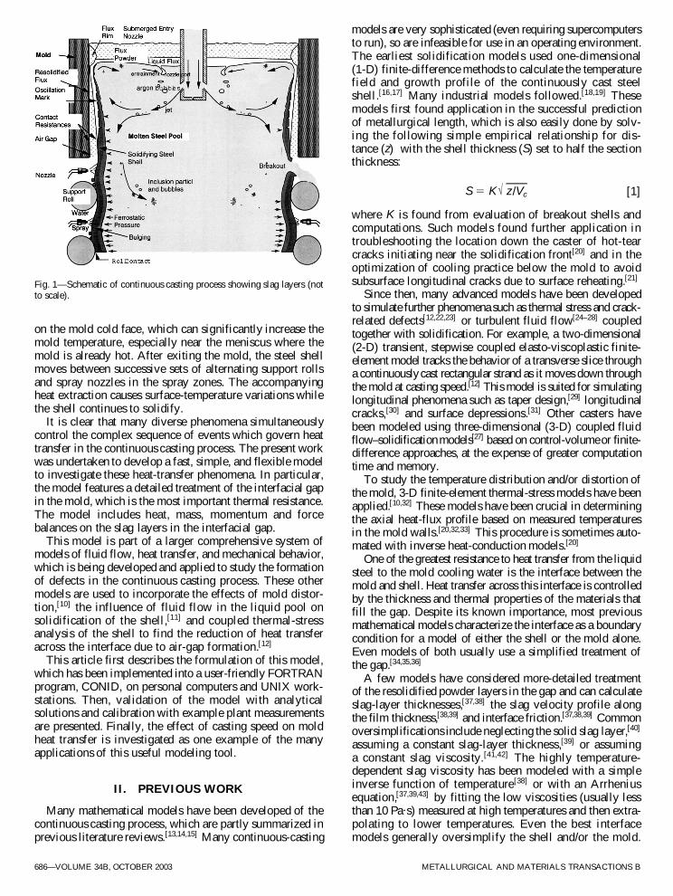
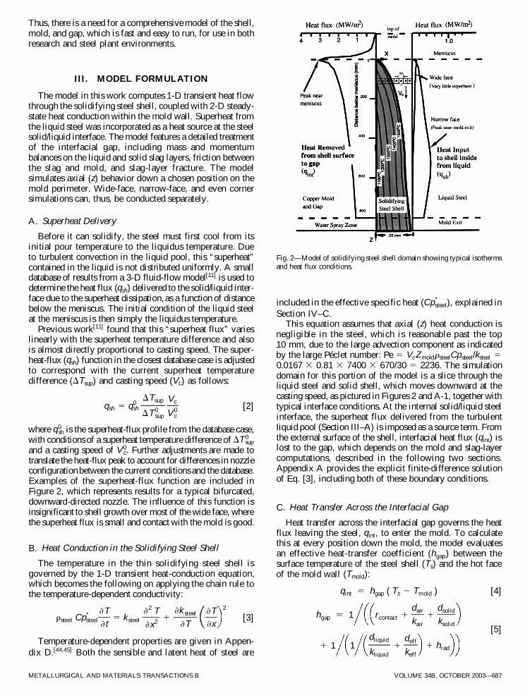
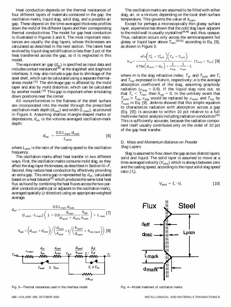
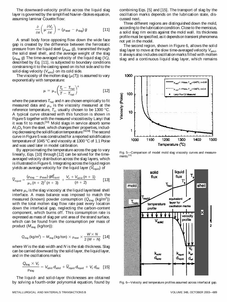
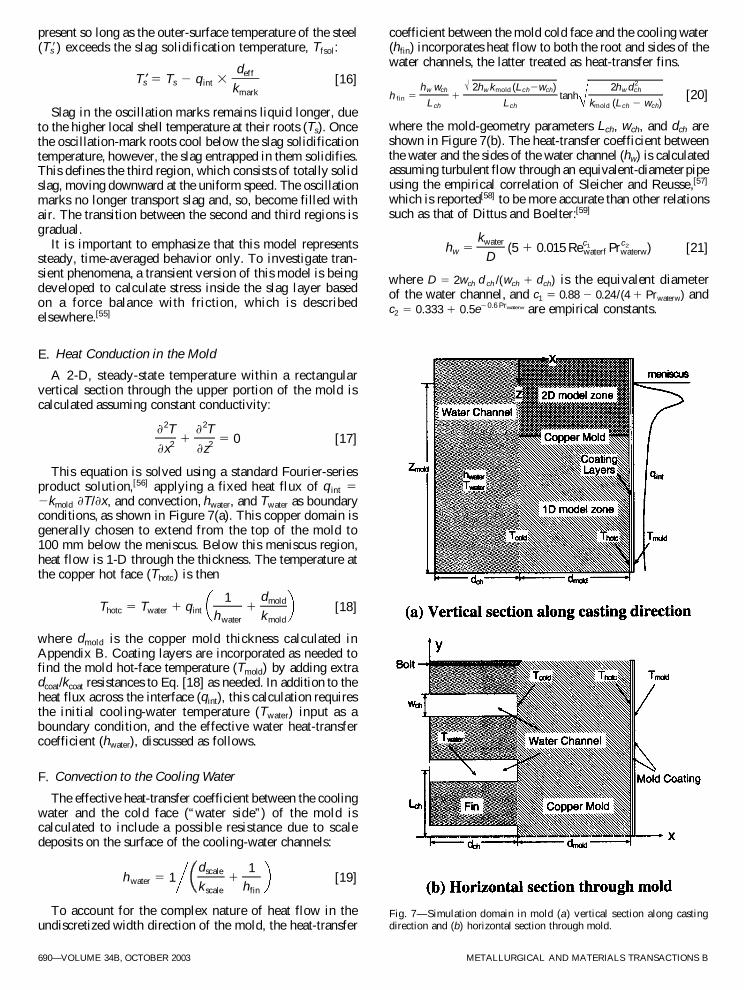
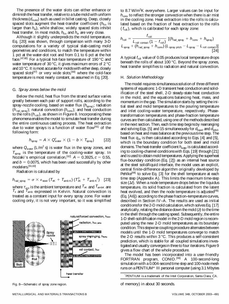
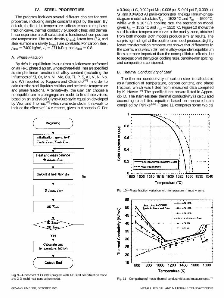
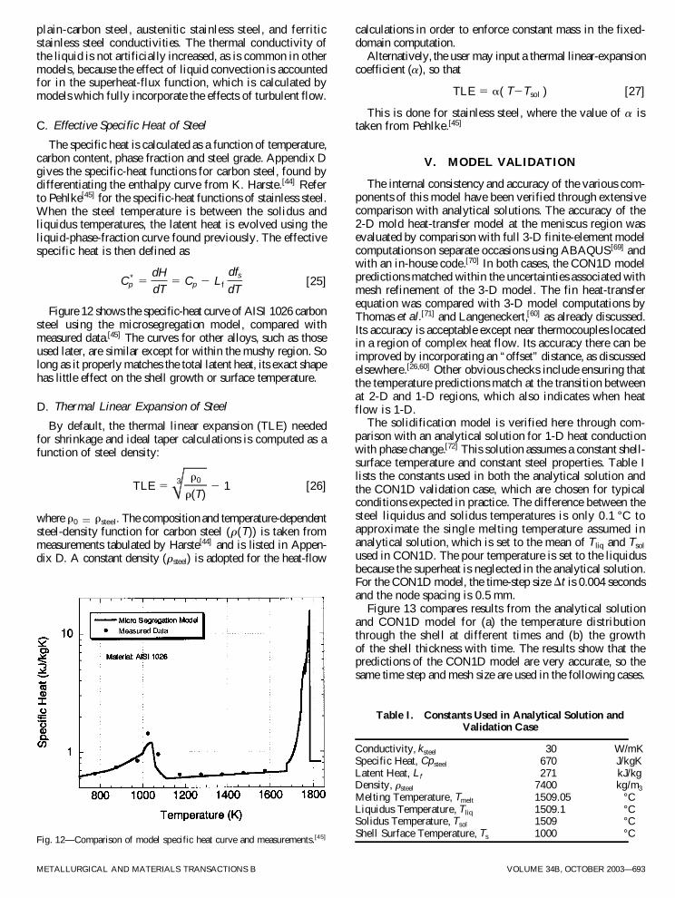
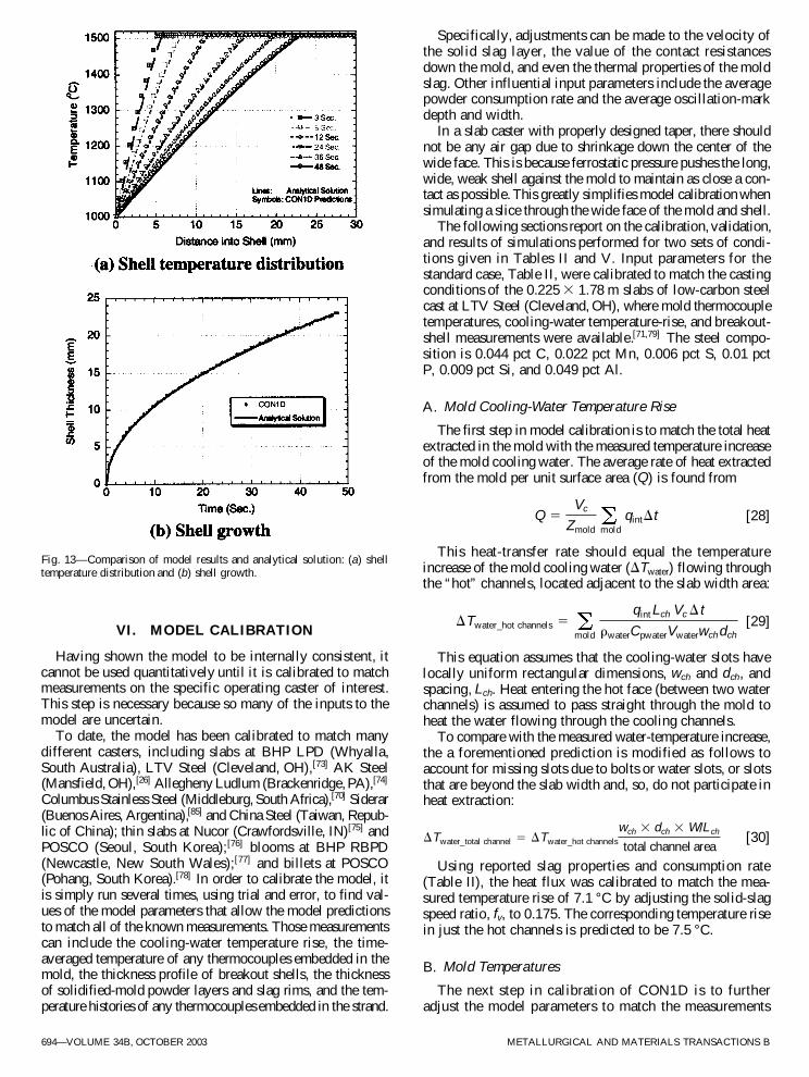
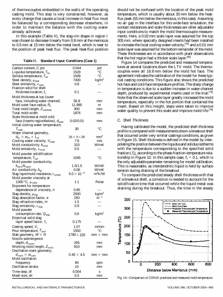
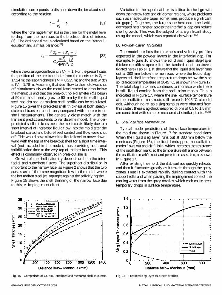
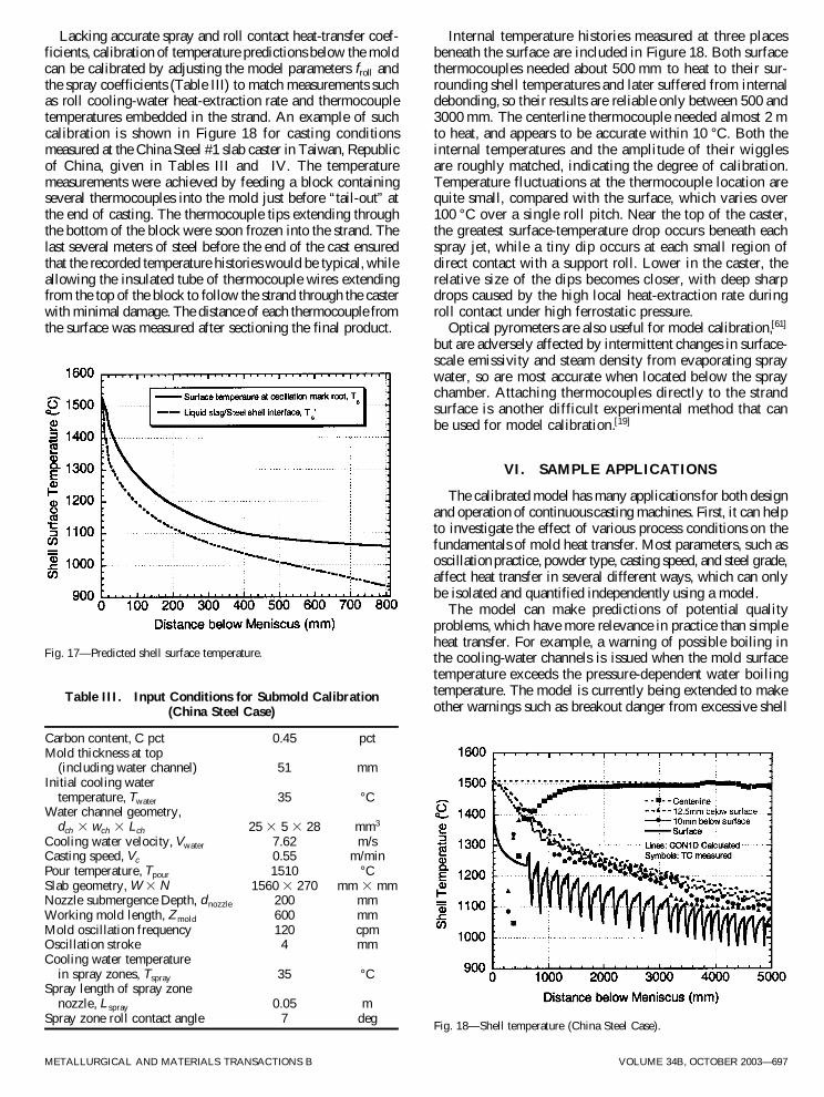
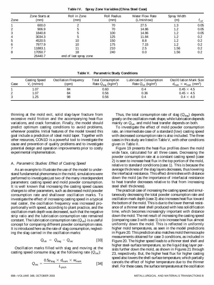
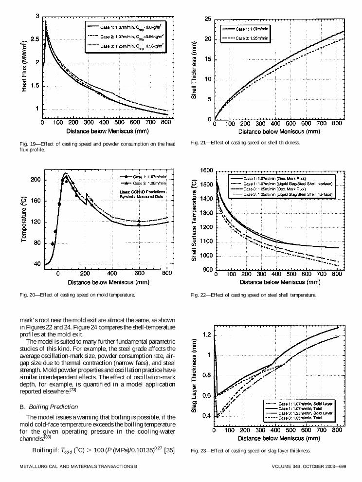
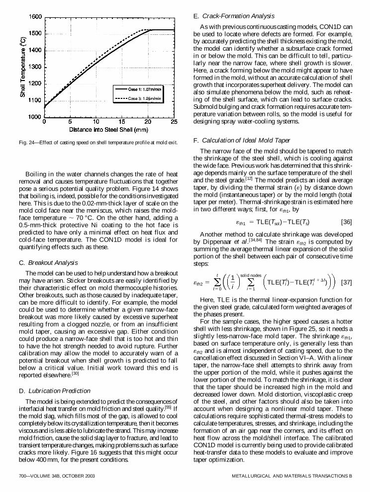
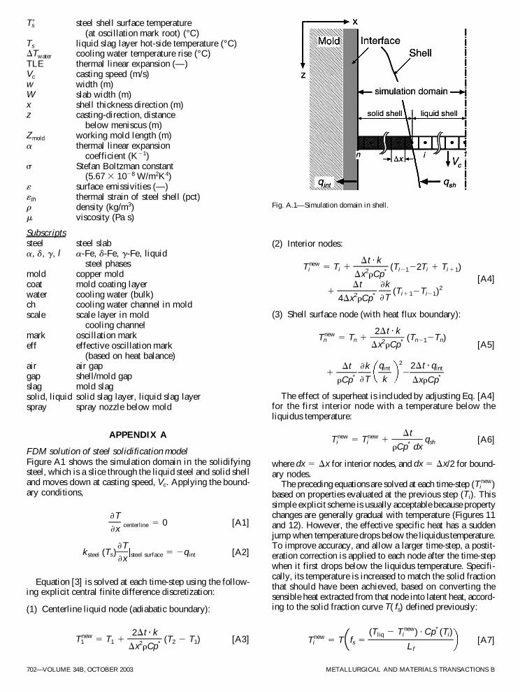
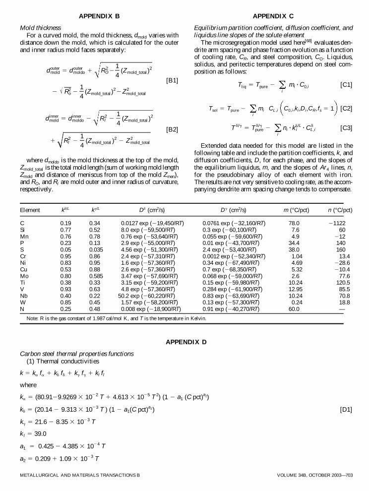
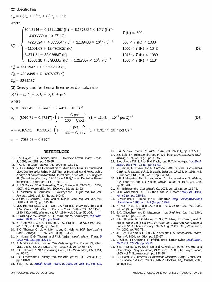