DI

SC

US

SI

ON

P

AP

ER

S

ER

IE

S

Forschungsinstitut zur Zukunft der ArbeitInstitute for the Study of Labor

Health, Height, Height Shrinkage and SES at Older Ages: Evidence from China

IZA DP No. 6489

April 2012

Wei HuangXiaoyan LeiGeert Ridder

John StraussYaohui Zhao

Health, Height, Height Shrinkage and SES

at Older Ages: Evidence from China

Wei Huang Harvard University

Xiaoyan Lei

Peking University and IZA

Geert Ridder University of Southern California

John Strauss

University of Southern California

Yaohui Zhao Peking University and IZA

Discussion Paper No. 6489

April 2012

IZA

P.O. Box 7240 53072 Bonn

Germany

Phone: +49-228-3894-0 Fax: +49-228-3894-180

E-mail: iza@iza.org

Any opinions expressed here are those of the author(s) and not those of IZA. Research published in this series may include views on policy, but the institute itself takes no institutional policy positions. The Institute for the Study of Labor (IZA) in Bonn is a local and virtual international research center and a place of communication between science, politics and business. IZA is an independent nonprofit organization supported by Deutsche Post Foundation. The center is associated with the University of Bonn and offers a stimulating research environment through its international network, workshops and conferences, data service, project support, research visits and doctoral program. IZA engages in (i) original and internationally competitive research in all fields of labor economics, (ii) development of policy concepts, and (iii) dissemination of research results and concepts to the interested public. IZA Discussion Papers often represent preliminary work and are circulated to encourage discussion. Citation of such a paper should account for its provisional character. A revised version may be available directly from the author.

IZA Discussion Paper No. 6489 April 2012

ABSTRACT

Health, Height, Height Shrinkage and SES at Older Ages: Evidence from China*

Adult height, as a marker of childhood health, has recently become a focus in understanding the relationship between childhood health and health outcomes at older ages. However, measured height of the older individuals is contaminated by height shrinkage from aging. Height shrinkage, in turn may be correlated with health conditions and socio-economic status from throughout the life-cycle. In this case it would be problematic to use measured height directly in regressions without considering such an effect. In this paper, we tackle this problem by using upper arm length and lower leg length to estimate a pre-shrinkage height function for a younger population that should not have started their shrinkage. We then use these estimated coefficients to predict pre-shrinkage heights for an older population, for which we also have upper arm and lower leg lengths. We then estimate height shrinkage for this older population and examine the associations between shrinkage and socio-economic status variables. We provide evidence that height shrinkage for both men and women is negatively associated with better current SES and early life conditions and, for women, positively with pre-shrinkage height. We then investigate the relationships between pre-shrinkage height, height shrinkage and a rich set of health outcomes of older respondents, finding that height shrinkage is positively associated with poor health outcomes across a variety of outcomes, with results for older age cognition being especially strong. Indeed height shrinkage is more strongly associated with later life outcomes than is pre-shrinkage height, suggesting that later life conditions are especially important correlates for these outcomes. JEL Classification: D1, I12, J13 Keywords: height, height shrinkage, health, China Corresponding author: Xiaoyan Lei China Center for Economic Research Peking University Beijing 100871 China E-mail: xylei@ccer.pku.edu.cn

* We would like to thank helpful advice and suggestions from Janet Currie, David Cutler, Richard Easterlin, Richard Freeman, Anastasia Gage, Amanda Kowalski, T. Paul Schultz and Yi Zeng. We are also indebted to the comments from Paul Frijters at the 32nd Conference for Australian Health Economists, Yiqing Xu at the 1st CCER Academic Conference, three discussants at the 10th China Economic Annual and suggestions from all the participants in CCER labor workshop. We are responsible for all remaining errors and omissions. This research is supported by National Institute of Aging, the Natural Science Foundation of China, Fogarty International Center, the World Bank, and the Peking University-Morgan Stanley Scholarship.

I. Introduction

The rapid aging of population places health at older ages among the top public

health priorities in recent years as the fraction of the population that is elderly has

been rising. In countries such as China, rapid aging has occurred at much lower

levels of national income and worse health conditions than was the case in

industrial countries. The elderly in such countries were children when economic

development and health conditions were far worse than today and their health as

adults is likely to have been a¤ected by such past conditions, more so than the

elderly in industrial countries.

The e¤ects of early-life health and environment on cognitive function, health,

wellbeing and mortality have been documented by researchers across a range of

disciplines, using data from many countries over the world (Elo and Preston, 1992;

Barker, 1994; Godfrey and Barker, 2000; Finch and Crimmins, 2004; Case et al.,

2005, 2008b, 2010a, b; Alderman and Behrman, 2006; Zeng et al., 2007; Van den

Berg, 2006; Smith, 2009; Huang and Elo, 2009, Almond and Currie, 2011).

There are several literatures that have used height to proxy for past health. In

the large historical literature, adult height is taken to be an indicator of population

health (Fogel, 1986, 2004; Steckel, 1995, 2009). The nutrition literature long ago

established that child height is a very good summary measure of overall health of

children (e.g. Martorell and Habicht, 1986). Adult height while re�ective of the

adolescent growth spurt, is also highly correlated with height during childhood.

A strong association has been found to exist among the elderly between

measured height and cognitive ability, self-reported health, illness status and

1

measures of depression (Case and Paxson, 2008a; Case and Paxson, 2010a; Deaton

and Arora, 2009; Heineck, 2008; Maurer, 2010; Smith et al., 2012). Most of this

literature is from industrial countries (Maurer, 2010 and Smith et al., 2012, are

exceptions). The exact mechanisms are not completely known, as these studies are

not structural, nor causal. Some of the pathway is likely to be through better

health during childhood and prime-aged adulthood (e.g. Case and Paxson, 2008b

or Smith, 2009), but other pathways exist as well, such as taller people having more

schooling and consequently making better health behavior decisions (e.g. Cutler

and Lleras-Muney, 2010).

However, older people su¤er height shrinkage during aging. Aging is associated

with several physiological and biological changes, including body composition, such

as an increase in body fat, a decrease in lean body mass and bone mass

(Kuchmarsk, 1989). Through such mechanisms as certain kinds of arthritis (such

as ankylosing spondylitis), in�ammation of spine joints, herniated disks, or

kyphosis, these changes can lead to vertebral deformity, which can contribute to a

reduction in height (Kwok et al., 2002; Prothro, 1993; Roubeno¤ and Wilson,

1993). One health condition that can in�uence shrinkage directly and through

many of these other proximate causes is osteoporosis. Osteoporosis, and some of

these other health factors, may well be associated with SES factors through

mechanisms such as early menopause, diet, exercise, smoking, excess drinking and

exposure to certain heavy metals such as lead. Height shrinkage may thus be more

severe in those with current health problems or problems from early childhood, or

even be correlated with pre-shrinkage height itself and with SES, leading to

2

potentially biased estimates of the impacts of height on other health measures in

OLS regressions. More to the point, there is little if any literature that explores

the SES correlates of height shrinkage.

While the problem height shrinkage may cause has been considered by some

researchers, there is little literature addressing it. One exception is Maurer (2010),

who addressed this problem by using lower leg length as an instrument for height

to address the measurement error problem, among urban elderly from Latin

America and the Caribbean. Many studies exist that show a strong correlation

between lower leg length, arm length and pre-shrinkage adult height (see below).

For Maurer�s estimator to be consistent, it is necessary that lower leg length is

conditionally uncorrelated with any height shrinkage. If it is so correlated, then

lower leg length will be correlated with the error term in the �rst stage regression,

which includes shrinkage. In this case, these IV estimates will be inconsistent.

In this paper, we use both estimated pre-shrinkage height and shrinkage as

covariates in OLS regressions, rather than instrumented height to tackle the

problem. The �rst step is to estimate the pre-shrinkage height of the seniors. This

issue has a long history in the nutrition and human biology literature, even,

especially, using cross-section data. Limb lengths are used to predict height and the

resultant prediction is used as a measure of pre-shrinkage height. This works

because the limbs used in this literature do not generally shrink as people age.

Lower leg length (Chumlea et al., 1985; Chumlea and Guo, 1993; Protho and

Rosenbloom, 1993; Myers et al., 1994; Zhang et al., 1998; Bermudez, 1999; Li et al.,

2000; Cheng et al., 2000; Pini et al., 2001; Knous and Arisawa, 2002), arm span

3

from roughly the shoulder to the wrist (Kwok and Whitelaw, 1991; Kwok et al.,

2002), total arm length (Mitchell and Lipschitz, 1982; Haboubi et al., 1990;

Auyeung and Lee, 2001), upper arm or humeral length, tibia length (Haboubi et

al., 1990) and �bula length (Auyeung and Lee, 2001) have all been employed to

estimate pre-shrinkage stature. Most of this literature simply uses lower leg or arm

length to predict height using older populations. Rarely is an attempt made to

estimate shrinkage and generally no attempt is made to relate shrinkage to

socio-economic variables, although see Hillier et al. (2012) for a recent, interesting

exception relating shrinkage in older women to subsequent hip fractures and

mortality.

Based on the national baseline data from the China Health and Retirement

Longitudinal Study (CHARLS), this paper investigates the correlates of shrinkage

with current SES and indicators of childhood health, and whether shrinkage is

correlated with preshrinkage height. We �nd strong negative associations between

shrinkage and current measures of SES such as level of education, log of household

per capita expenditure (pce), urban residence, as well as strong correlations with

county of current residence and province of birth. However the correlation between

height shrinkage and non-location measures of childhood background are weak.

We also �nd signi�cant, positive correlations between shrinkage and preshrinkage

height for women, suggesting that the IV strategy discussed above is not valid for

women in the CHARLS data.

We then replace measured height by our pre-shrinkage height estimates, plus

our estimates of height shrinkage, as covariates in regressions to investigate their

4

associations with a rich set of later-life health variables: measures of cognitive

functioning, hypertension, lung capacity, grip strength, balance, walking speed,

self-reported general health, measures of physical functioning, activities of daily

living (ADLs), instrumental activities of daily living (IADLs), the Center for

Epidemiologic Studies- Depression (CES-D) scale and expectation of surviving to

age 75 (for respondents under 65). We �nd that even controlling for SES and early

life health conditions, that pre-shrinkage height and especially height shrinkage

have signi�cant associations with these later life health conditions. In general

height shrinkage is negatively correlated with good health outcomes and

pre-shrinkage height positively so. Given that height shrinkage is a marker for

later-life health problems, in contrast to pre-shrinkage height which is a marker of

early life health, this evidence means that it is not only early life events that are

associated with late life health outcomes (childhood background variables are

jointly signi�cant in these health regressions), but health insults in later life as well.

By providing the evidence of whether and how height shrinkage is correlated with

health, pre-shrinkage height and SES, this paper also validates the concern raised,

but not tested, by Case and Paxson (2008a) that individuals with poor health tend

to shrink more than healthy ones..

This paper is organized as follows. In Section II we discuss our model and

econometric framework to estimate height shrinkage and preshrinkage height.

Section III discusses the data used in this paper and summary statistics. Section

IV shows how we estimate the pre-shrinkage height function from a sample of

"young" respondents and height shrinkage for our "older" sample. Section V

5

discusses the evidence on the association between height shrinkage and SES and

pre-shrinkage height. Section VI provides further evidence on the association

between height shrinkage, pre-shrinkage height and our health measures of this

older population. Section VII concludes.

II. Theoretic Framework

In previous studies, what has interested many researchers is the association

between height and health status. A prototypical regression is:

y = x0� + p� + u (1)

in which y stands for health variables like self-reported health, ADL disability or

cognitive ability; p is respondents�preshrinkage height; x is short for a set of

co-variates, such as demographic variables, possibly SES, or perhaps other

childhood health variables; u is the error term, which is assumed in the literature to

be mean independent of height and control variables. We also assume that it is

mean independent of the predictors of pre-shrinkage height.1 Most researchers are

interested in the coe¢ cient �. However, in most situations, pre-shrinkage height is

unobserved and the interviewers have available only measured height (h), which

might have been contaminated by height shrinkage (s). The regression thus

estimated is:1Of course even height, though predetermined, will be correlated with unobserved variables so

that the regression coe¢ cients in (1) are not causal e¤ects.

6

y = x0e� + he�+ eu (2)

and for the older population measured height (h), as an identity equals

pre-shrinkage height (p) minus height shrinkage (s) (in the younger sample, in

principle, measured height equals preshrinkage height):

h � p� s (3)

Height shrinkage may be independent of pre-shrinkage height, which is easier

to handle, but this may not be the case. On the one hand, pre-shrinkage height is a

marker of early life health status, and healthier people might shrink less with aging,

have less osteoporosis for example. On the other hand, taller people may lose more

height if they su¤er kyphosis or some other related diseases. In these situations, the

coe¢ cients on height and x in (2) are a biased estimate of the coe¢ cients on

preshrinkage height and x in (1) because the error in (2) will contain shrinkage that

is correlated with pre-shrinkage height and x.2

Maurer (2010) assumed that lower leg length was correlated with pre-shrinkage

height and not correlated with height shrinkage, and used lower leg length as an

instrument for measured height. Then he argued that the 2SLS estimation would

give consistent results. However, if pre-shrinkage height is correlated with height

shrinkage conditional on control variables and error term, then this 2SLS estimate

will also be inconsistent.2In Section V, we will provide some evidence that height shrinkage is correlated both with SES

and with pre-shrinkage height, thus with the error term, ":

7

In this paper, we use lower leg length and upper arm length to predict

pre-shrinkage height using di¤erent data on a younger population, instead of taking

them as instruments directly. We use estimates of this height function to predict

pre-shrinkage height and height shrinkage for respondents from an older

population, aged 60 and over.

Firstly, we estimate the following equation for the younger group:

hy = z0y + �y (4)

where z is a vector representing lower leg length, upper arm length (as an adult)

and a Han ethnic dummy. The variables in x and z overlap because of the Han

dummy, but there are variables (the limb lengths) in z that are excluded from x.

We assume

E(�yjzy; xy) = 0

We then apply the estimated coe¢ cients to the older age-group to estimate their

pre-shrinkage height:

bpo = z0ob (5)

Height shrinkage is de�ned as the di¤erence between pre-shrinkage height and

measured height, as in (3).

After estimating pre-shrinkage height and height shrinkage, we estimate the

association between height shrinkage and SES variables, i.e. education levels, per

capita pce, age dummies, living in an urban area, marital status and childhood

8

background variables: having an urban childhood upbringing, schooling of each

parent, whether each parent had died before the respondent was 18, a self-reported

general health measure of the respondent�s health before age 16 and dummies for

province of birth.3 In a second speci�cation we add pre-shrinkage height. That is:

s = x0� + p� + " (6)

with E("jx; p; z) = 0. Finally, we estimate (1) and (2), along with (7) below, to

examine the associations between height and health:4

y = x0� + p� + s�+ u (7)

Separate OLS estimation of (4) and (6), or (4) and (7), is the optimal 2-step

GMM estimator. Our standard errors for (1), (6) and (7) are corrected for the fact

that we use predicted variables as dependent and/or independent variables. We

derive the asymptotic variances in the appendix.

3The childhood background variables might be thought of as possible instrumental variables forlimb lengths in (4), however this would require the assumption that the only in�uence of childhoodbackground on pre-shrinkage height, height shrinkage and other height outcomes, is through limblengths, which is not consistent with the recent literature on early childhood-later life health associ-ations. In results not shown, apart from women having an urban upbringing for upper arm length,only the province of birth dummies are signi�cantly related to limb lengths, among the childhoodbackground variables available to us.

4Note that if we estimated (1), estimating pre-shrinkage height on the older sample, we wouldbe using 2SLS, as in Maurer (2010). We would face the same issues we raised above.

9

III. Data

The China Health and Retirement Longitudinal Study (CHARLS) was

initiated to study the elderly population of China. It is designed to be

complementary to the Health and Retirement Study (HRS) in the United States

and like surveys around the world. CHARLS covers 150 counties randomly chosen

across China. Twenty-eight provinces are represented in the data.5 Counties were

grouped into 8 geographic regions, and strati�ed by rural/urban status and by per

capita county GDP.6 Counties were then sampled, strati�ed, with probability

proportional to population (pps).7 Within counties we sampled three

administrative villages or urban neighborhoods (resident committees) as our

primary sampling units (psu), again using pps.8

The sampling goal within primary sampling units was 24 households with an

age eligible member, de�ned as a person aged 45 or older. Sampling rates varied

by psu. We �rst mapped all of the dwellings in the psu, using Google Earth maps,

adjusted from the ground by our mapping teams.9 From this we obtained a

sampling frame of dwelling doors. We then randomly sampled 80 doors, and

5Tibet was excluded from the study. Two other provinces, Hainan and Ningxia, both very smallin population size, are not represented among the CHARLS counties..

6Data sources were the Population Statistics by County/City of PRC, 2009 (data from 2008)and the provincial statistical yearbooks (for GDP per capita).

7This was done by listing the strati�ed counties and selecting counties with a �xed interval andrandom starting point. This way we ensure that all parts of the GDP per capita distribution arecovered.

8Data on population sizes were provided by the National Bureau of Statistics (NBS).9CHARLS mapping sta¤ �rst went to the areas with GPS devices and took readings of the

administrative boundaries, which were used to extract the Google Earth maps. A few primarysampling units had unreadble or no Google Earth maps, in which case we constructed the mapsfrom the ground. In all cases we checked the maps from the ground and added to them when theywere not up to date.

10

obtained information on the age of the oldest person and whether the dwelling was

vacant (which some were). Using this information, we calculated age eligibility

rates. From this information we determined psu-speci�c sampling rates to ensure

in expectation 24 age-eligible households and re-sampled from the initial dwelling

list. If a dwelling had multiple households living in it, we randomly sampled one

with an age-elgible person. Households were de�ned as living together, sharing

meals and at least some other expenses. After sampling our �nal list of

households, we again checked for age eligibility and then randomly sampled one

person age 45 or over, and their spouse (no matter the age), as our respondents.

The national baseline was �elded from late summer 2011 until March 2012 (see

Zhao et al., 2012, for details). Among all households, the age eligibility rate was

62% and the response rate among eligible households was 84%; 90% among rural

households and 77% for urban households.10 These rates compare very well with

other HRS surveys in their initial waves. Sample size is 17,085 individuals with

non-missing ages.

We use two samples for this paper. We estimate our preshrinkage height

prediction equation using a "young" sample of respondents and spouses aged 45-49,

who have presumably not started to shrink yet, or if so, have only shrink a very

small amount on average. We then use respondents and spouses aged 60 and over

to predict preshrinkage heights, calculate shrinkage and estimate our models. Of

the 17,085 observations, 3,027 are between 45 and 49 and 7,611 are 60 and over.

Approximately 15% of "young" respondents did not get their biomarkers taken,

10Of those who did not respond, about half refused and half could not be found.

11

usually because they were busy at work and unavailable. Among the "old" sample,

18% did not get any biomarkers taken, usually because they were too frail to be

measured. Non-measurement rates were higher among those over 80 years. In

addition, some observations were dropped because they had missing heights or

other key variables missing or out of reasonable range. We are left with 1,101 men

and 1,508 women in the "young" sample and 2,940 men and 2,928 women in the

"old" sample, who have complete height and limb measurements (fewer with all of

the other health variables complete).

Anthropometric measures included respondent�s standing height, upper arm

length and lower leg length, all measured in millimeters. The summary statistics of

these variables are shown in Panels A and B of Table 1 for the "young" and "old"

samples, respectively. Height was measured using a stadiometer directly from the

heel to the top of head with the elders standing up-right. Upper arm length was

measured with a Martin caliper with the respondent standing and holding the left

or right arm at a right angle. We measured from the acromion process of the

scalpula to the olecranon process. Lower leg length was also measured using a

Martin caliper from the right knee joint to the ground. Measured heights are

smaller for the older group, by some 4 cm for men and 4.5 cm for women. Much of

this di¤erence could be due to shrinkage, although it could also be that older birth

cohorts were less tall. Comparing upper arm lengths, they are very close between

the 45-49 and 60 and over groups, suggesting that shrinkage may be the more

important explanation. On the other hand, lower leg lengths are about 0.6 cm

smaller for the over 60 group, for both men and women, suggesting some possible

12

cohort e¤ects.

As mentioned above, this study examines the associations between

pre-shrinkage height and height shrinkage on di¤erent measures of health of older

people. We start with cognition questions, which are grouped into three, following

McArdle (2010) and Smith et al. (2011). The �rst component is the Telephone

Interview of Cognitive Status (TICS). There are ten questions in this part, from

awareness of the date (using either solar or lunar calendar), the day of the week

and season of the year, to successively subtracting 7 from 100. An index is formed

of the number of correct answers. This is a measure of the mental intactness of the

respondent (Smith et al., 2011). A second set of questions asks a respondent to

recall a series of 10 simple nouns and to recall again after approximately 10

minutes. Following McArdle (2010), we average the number of correct answers as

our dependent variable. This is a measure of episodic memory, and is a component

of �uid intelligence (Smith et al., 2011). Finally respondents are shown a picture

of two overlapping pentagons and asked to draw it. We score the answer as 1 if the

respondent successfully performs this task.

We have several biomarker variables available. We measure blood pressure

three times. We create a dummy variable equal to one if a respondent has

hypertension. For this case we take means of systolic and diastolic measurements

and assign a hypertensive status equal to one if mean systolic is 140 or greater or if

mean diastolic is 90 or greater. In addition respondents self-report if they have

been diagnosed by a doctor with hypertension and we include those cases as being

hypertensive. Respondents blow into a peak �ow meter three times to measure

13

lung capacity and we take the average. Respondents have their grip strength

measured by a dynamometer. Two measurements are taken from each hand. We

use average measurement from the self-reported dominant hand. Respondents are

given a balance test, whether they can stand semi-tandem or full tandem. Because

most can stand full tandem, we create a dummy equal to 1 if they can do so.11

Finally we conduct a timed walk of 4 meters, asking the respondent to walk at a

"normal" speed.

The remaining health measures are self-reported. General health is reported

on a scale: very good, good, fair, poor, very poor. We construct a binary variable

equal to one if health is reported as very poor or poor, zero otherwise. Respondents

are asked about whether they have di¢ culty in performing certain classes of

activities: physical functioning, ADLs and IADLs.12 We count the number of items

in each group that the respondent claims having di¢ culty in performing or cannot

perform. The expected survival question asks respondents to rank their

expectation of surviving to a speci�c older age on a �ve point scale, from almost

impossible to almost certain. We group the bottom two answers, almost

impossible and not very likely. Because di¤erent age groups are asked survival

chances to di¤erent ages, we standardize by only using those respondents under age

65, who are asked their survival chances to age 75. Similarly, respondents

answered a Chinese version of CES-D 10 questionnaire in the survey, which

11Respondents under 70 are asked to stand in full tandem for 60 seconds, those 70 and over for30. We include age dummies as covariates, which will capture this di¤erence.12There are nine questions on physical functioning, ranging from having di¢ culty running or

jogging 1 km, to walking 1 km, tocarrying a heavy bag of groceries, to picking up a small coin.There are 6 ADL questions(eg. getting into and out of bed or using the toilet) and 5 IADL quesitons(eg. doing household chores, shopping, or managing money).

14

contained 10 questions about the respondents�depression status. Based on that, we

constructed a CES-D scale, with range from 0 to 30.

Mean values and standard deviations of all the health variables are provided in

Panel B of Table 1 for the "old"sample. As is generally the case, health measures

for older women are worse than for men. This is true both for self-reported

measures such as poor general health, di¢ culties with physical functioning or

ADLs, and the CES-D depression scale, and for biomarkers such as hypertension,

the cognition measures, grip strength and lung capacity.

Panel B also reports summary statistics of demographic variables like

education level, log of household per capita expenditure (pce),13 marital status and

type of areas (urban/rural) where respondents live at the time of the survey. The

current generation of elderly population in China has only a small amount of

schooling, particularly among women. Fifty-�ve percent of women 60 and over are

illiterate, twenty percent among men. Only 8% of older men and 3% of women

have completed senior high school or more. However, 56% of men have completed

primary school, and 35% of women. When we compare these numbers to the

parents of these elderly, some progress had been made, since over 70% of fathers

and 90% of mothers are reported to be illiterate (no schooling or less than primary

school completion-see Panel B). The preponderance of our respondents are still

married, more so among men, since their spouses tend to be younger. An

overwhelming majority, over 80% of older men and women, live in rural areas.

13Per capita expenditures include the value of food consumed from own production. We preferpce to income because pce is measured with less error and better represents long-run resources,since households smooth their consumption over time.

15

Childhood background variables are also reported in Panel B. An even larger

percent, over 90, have a rural background as a child. About 10-12% of fathers

died before the respondent was age 18 and about 6-7% of mothers. CHARLS has a

retrospective question about general health before the respondent turned 16 (an

average over that period), with categories excellent, very good, good, fair or poor.

This has been successfully used by HRS and other aging surveys, including the

CHARLS pilot, and has been linked to later life health outcomes (e.g. Smith,

2009). In the CHARLS sample, 6% of men and 9% of women report that their

childhood health was poor. Finally CHARLS also elicits province of birth.

Evidence on public health infrastructure for pre-revolutionary China is scant, but

some evidence exists that in Beijing, better water and sanitation facilities were

built between 1910 and 1920 (Campbell, 1997) and that led to a rapid decline in

infant mortality in there. This would have a¤ected our cohorts. For other major

cities there is some, but not much, evidence that public health infrastructure was

being built during that time period (Campbell, 1997).

IV. Estimation of Pre-shrinkage Height

Following the methodology in the medical literature, we use lower leg length

and upper arm length and estimate gender-speci�c equations using measured

height as the dependent variable. Additionally, we add quadratics in both limb

lengths and interactions to allow for nonlinearities. We also add a Han dummy

variable to pick up potential ethnic di¤erences.14

14Ethnic di¤erences in the proportions of limb lengths to height have been found in the literature(see Steele, 1987, for example). Age is not included. Age itself should only have an in�uence on

16

The steps to estimate pre-shrinkage height is as follows: �rst, we use data from

the "young" group, aged 45-49, and regress measured height on lower leg length,

upper arm length, their squares and interaction and the Han dummy. These

coe¢ cients are then applied in the "older" sample, those aged 60 and above, and

the predicted value is the estimated pre-shrinkage height for this group. Some

medical studies have used this approach, separating "young" and "old" groups,

include Steele (1987) and Reeves et al. (1996).15 A strong assumption is required

that any secular changes in height across birth cohorts (which are important in

China) do not change the relationship between height and limb length (see Leung

et al., 1996 and Kwok et al., 2002).16 The regressions are shown in Table 2.

Columns (1)-(3) in Table 2 show the coe¢ cients of the pre-shrinkage height

function in the male sample and columns (4)-(6) for the female sample. We �rst

show a linear speci�cation in limb lengths and the Han dummy, then add

quadratics and an interaction, and �nally a linear time trend. The quadratics and

interaction are always jointly signi�cant at under .001, while the time trends are

not signi�cant at standard levels; hence we use columns (2) and (5) as our preferred

estimates. The marginal e¤ects on height of both lower leg and upper arm lengths

are positive over the entire distribution, and convex. The Han dummy is positive

pre-shrinkage height through birth cohort e¤ects. These are likely but the sample we estimate ourcoe¢ cients for only spans 10 years. We do try one speci�cation that includes a linear trend in yearof birth, but it is never signi�cant at standard levels.15However, most of the medical literature estimates the coe¢ cients using the same age-group

sample as is used to predict preshrinkage height.16Kwok et al. (2002) use data on an older sample in China to estimate their prediction equation,

but they �rst remove observations who have symptoms of vertebral deformity based on x-ray images.They �nd the same ratio of total arm span to height for younger and older men, but a slightly higherratio for older women.

17

for both men and women, but signi�cant (at 5%) only for women. The R2�s are

over .51 for both men and women.17

After we obtain our pre-shrinkage height estimates for the 60 and older group,

height shrinkage is de�ned as the estimated pre-shrinkage height less the current

measured height. The summary of our estimates are shown in Panel B in Table 1.

Mean height shrinkage is 3.3 cm for men and 3.8 cm for women, which is consistent

with �ndings in the human biology literature that women have more problems with

vertebral deformity (see Kwok et al., 2002).

Figure 1 shows the age pattern of measured height, pre-shrinkage height and

height shrinkage by gender. The top two �gures show non-parametric graphs of

measured height and pre-shrinkage height as a function of age. And the bottom

two graphs show the pattern of height shrinkage and age for males and females

respectively.18 From the top two graphs, estimated pre-shrinkage height does not

decline much with age, a little more for men than for women. However measured

height does decline with age, indicating that height shrinkage increases, as shown in

the bottom two �gures. Our pre-shrinkage height estimates do not correct for

mortality selection. If we assume that respondents who survived to older ages are

those who were taller and less frail, then adding those who died back would result

in pre-shrinkage heights declining with age. This is what we would expect if older

birth cohorts faced worse health conditions at birth, and in early life.

17Many of the medical papers obtain higher R2s for their height prediction equations, but theygenerally have extremely small samples and extrememly controlled circumstances in which themeasurements are conducted, which should minimize measurement error, compared to a large-scalepopulation survey such as CHARLS..18The non-parametric curves are calculated using a Jianqing Fan (1992) locally weighted regres-

sion smoother, which allows the data to determine the shape of the function.

18

As a check on our preshrinkage height estimates, we compare our CHARLS

preshrinkage heights for the sample aged 60-69 in 2011, by year of birth, to

measured heights in another data source, the China Health and Nutrition Survey

(CHNS). We use the same birth year cohorts in both data sets, but in the CHNS

data, we can measure heights of these cohorts 20 years earlier, in 1991, when they

would be aged 40-49, and so should not have begun to shrink much yet. We thus

expect their measured heights in 1991 to be close to our estimated preshrinkage

heights in the CHARLS data for the same birth year cohort.19 The CHNS data in

1991 only covers 8 provinces, not 28 provinces as in CHARLS, and so is not

representative of all of China, in contrast to CHARLS, which should be born in

mind. We use the entire CHARLS sample for comparison in order to have a larger

sample size. The results are shown in Appendix Table 1. Comparing mean

heights by birth year cohort between being measured in 1991 in CHNS and in 2011

in CHARLS, heights in 1991 are higher, by 1.5-4 cm, depending on the age, which

is consistent with shrinkage. Comparing mean heights in 1991 with estimated

preshrinkage heights from CHARLS, the results show a close correspondence. For

women, the di¤erences between the CHARLS estimated preshrinkage heights and

the CHNS measured heights is very small, generally under 0.7cm and often less

than 0.5cm. For men, aged 60-64 in 2011 (40-44 in 1991), the di¤erences are very

small as well; they increase some for those aged 65-69 in 2011, which may indicate

19We thank David Cutler for this idea. Note that the CHNS data do not include limb lengths, sowe cannot use the CHARLS preshrinkage height function estimates to predict individual preshrink-age heights with CHNS observations. Also only one height observation per person is available inCHNS, so it is not possible to take di¤erences in height measurements to measure shrinkage directly.

19

that there is some shrinkage that has begun in this age group.20

V. Height Shrinkage, Pre-Shrinkage Height and SES

Very few studies have been able to measure height shrinkage and we know

precious little about the correlations between shrinkage and later life SES, early life

health conditions and family background. Further, as noted, any correlations

between height shrinkage and upper arm and lower leg length are important since

they determine whether an IV estimator using lower leg and upper arm lengths as

IVs for measured height in health equations is consistent. Table 3 shows the

gender-speci�c results of the association between SES, early life conditions, upper

arm and lower leg length, and height shrinkage. All regressions control for basic

demographic variables, including dummy variables for age, Han ethnicity, marital

status, urban residence and current residential county. We also include covariates

measuring early life conditions, including dummies for province of birth, urban

upbringing before age 16, for schooling of the father and mother, for whether the

father and mother died by respondent�s age 18, and for whether the respondent

reported being in poor health on average before age 16. In columns 2 and 4 we add

preshrinkage height. All estimates correct standard errors for the fact that we

predict shrinkage and pre-shrinkage heights (see the Appendix for detailed

derivations).

From these estimates, we �nd that the SES variables are very important

predictors of height shrinkage; the Wald tests are all highly signi�cant. Dummy

20Plotting the ratio of lower leg or upper arm length to measured height in the CHARLS datadoes show a slight increase for those in their late 40s, which is consistent with this conjecture.

20

coe¢ cients of level of education are negative, monotonically declining with higher

education and jointly signi�cant. One potential explanation can be that people with

higher education level are more likely to have had better health behaviors when

younger. They are also likely to have had better health during childhood, perhaps

in ways not measured by our childhood general health variable. Household log pce

is negatively associated with height shrinkage, especially for men, indicating that

higher income people may be able to purchase better medical care and nutritious

food for themselves, although there is likely to exist reverse causality as well, which

may explain why the coe¢ cients are more negative for men. Being currently

married is associated with less shrinkage for men, but not signi�cant. Marriage is

often found to be correlated positively with better health and more happiness, and

is associated with better labor market outcomes for men, so this is not surprising,

though, again, we must remember that these estimates are not necessarily causal.

Not surprisingly, there are very strong positive associations between shrinkage and

age. Currently living in an urban area is signi�cantly associated with less

shrinkage for both men and women. The county dummies are jointly signi�cant at

under the .001 level. This is consistent with results such as Strauss et al. (2010),

who �nd very strong community e¤ects on health outcomes for the elderly in

China, using the CHARLS Pilot data. Early childhood background and health are

not jointly signi�cant in these regressions. However, having had poor childhood

health is associated with more shrinkage for women, signi�cant at 10%. Dummies

for birth provinces are jointly signi�cant, for both men and women.

Table 3 also demonstrates positive and signi�cant correlation between height

21

shrinkage and preshrinkage height for women, although not for men. This is

di¤erent from the results of Kwok et al. (2002), who �nd a weak negative

correlation for men; although those results are bivariate, not multivariate,

controlling for SES variables, as ours. This implies that lower leg and upper arm

length fail the IV requirement for women, that they be uncorrelated with the error

term (which includes shrinkage) in a health equation with measured height as a

covariate.

VI. Results: Impact of Estimated Height on Health Outcomes

Since there is a growing literature, cited above, that investigates how height is

associated with other adult health outcomes, it is of interest to explore this with

our estimates of preshrinkage heights and height shrinkage. We do not claim

causality from these regressions, because of the usual problem of omitted variables,

but also because in some instances reverse causality is possible.21 The procedure is

to regress our health measures �rst on measured height and control variables to get

our baseline estimates. Then we replace measured height by predicted

pre-shrinkage height and �nally add height shrinkage. Standard errors are again

corrected for predicted shrinkage and preshrinkage heights. Since some health

outcomes are missing for some observations, the number of observations di¤ers by

outcome.

Table 4.1-4.3 show the results from the regressions of our health measures on

21One potential example is with the depression score and shrinkage. Depression is associated inwomen with early menopause. Menopause in turn is associated with osteoporosis, which can leadto shrinkage. Now our depression score is current and may not indicate past episodes, but we alsoknow that if a person has had one bout of depression, that increases the likelihood of more, later.

22

height. The same demographic and SES controls, and controls for early life

conditions that we use in Table 3 are added in all the regressions. We start with

the cognition outcomes in Table 4.1. Measured height is positively and

signi�cantly associated with all of the cognition measures for both men and women.

Case and Paxson (2008a) �nd such relationships among the older population in the

United States using the Health and Retirement Study (HRS) (see Smith et al.,

2012 for evidence on China). A likely mechanism for this relationship is the

positive association between childhood height and childhood and later cognition.

There exists a large literature on early child height impacts on later child cognition;

Case and Paxson (2008b) is a recent example (see Glewwe and Miguel, 2008 and

Strauss and Thomas, 2008 for reviews). Since childhood heights are strongly

related to adult heights and cognition skills persist from childhood through

adulthood, it is not surprising to see this relationship among older persons. When

we replace measured heights by preshrinkage heights and height shrinkage,

preshrinkage height has the same positive, signi�cant association with the TICS

and draw a picture variables, though not for the word recall. Height shrinkage is,

however, strongly, negatively correlated with all of these measures and for both

men and women, suggesting that a part, perhaps a large part, of the association

between measured height and cognition occurs through height shrinkage. As we

saw in Table 3, shrinkage is highly associated with many current SES variables and

with some childhood background factors having to do with province of birth, and

for women, health as a child, but not with other measured childhood background

factors. Current and childhood SES and childhood health variables are each

23

jointly signi�cantly associated with the cognition outcomes, as are the current

county of residence dummies and, for women, the birth provinces. So these results

imply that later life cognition and health is associated with health events

throughout the life cycle and in later life, not just from early childhood.

In Table 4.2 we show results for the biomarkers. Preshrinkage height is

signi�cantly, positively related to lung capacity and grip strength, and height

shrinkage is signi�cantly, negatively related to both outcomes. Men who have

shrunk more take more time to do the timed walk, but for women shrinkage and

preshrinkage heights are not related to walk time. Hypertension and ability to

balance are also unrelated to both preshrinkage height and shrinkage. Current and

childhood SES are related to many of these outcomes, as are current county of

residence and province of birth.

Table 4.3 has results for self-reported health outcomes. As can be seen,

shrinkage is generally related to worse outcomes. For men, this is so for the CES-D

depression index, the likelihood of not surviving to age 75 (for those 65 and

younger), the number of measures of physical functioning that the respondent

reports having di¢ culty with, and having poor or very poor general health. For

women, shrinkage is signi�cantly associated with having more di¢ culties with

measures of physical functioning, ADLs and IADLs. What is surprising about these

results is that preshrinkage heights sometimes have positive associations with bad

health outcomes for women, although not for men. This is very unlike the results

for cognition and the biomarkers. Mortality selection could be partly causing this,

but we cannot be more than speculative on this point.

24

VII. Conclusions

According to Barker (1994), childhood health in uterus has a lasting impact on

health, including at old ages. Height has been used widely as an indicator in part

of childhood health. However, because height shrinks with aging, it su¤ers a

measurement error problem when studying its impact on health outcomes at older

ages.

Based on unique data of Chinese aged 45 and older, we address this problem

by making use of upper arm and lower leg lengths to construct estimates of the

relationship between these limb lengths and measured height, on a population aged

45-49, and then use these estimates to estimate preshrinkage height and height

shrinkage on a population 60 years and older. We then investigate the association

between height shrinkage, SES variables and variables measuring di¤erent

dimensions of childhood health. We follow this exercise by examining the

associations between measured height on the one hand, or pre-shrinkage height and

shrinkage on the other, and a rich set of health variables, including measures of

cognition, biomarkers, as well as various self-reported health measures.

The results in this paper show that shrinkage and socio-economic variables

such as schooling and household per capita expenditure are negatively correlated

for both men and women. Shrinkage is somewhat larger for women, which is

consistent with the medical literature. Shrinkage also depends positively on

pre-shrinkage height for women, which rules out a potential instrumental variables

strategy to correct measured height for omitted variables bias when it is used as a

covariate explaining other health variables, supporting the concern expressed in

25

Case and Paxson (2008a). Height shrinkage, and to a lesser extent, pre-shrinkage

height, are also correlated with many later life health outcomes, particularly

cognition and biomarker measures. In general the more the shrinkage the worse

are these other health outcomes.

26

Appendix: Asymptotic Variances

Table 3 uses a constructed dependent variable, height shrinkage, while Tables

4.1-4.3 use predicted preshrinkage height and, in some speci�cations, height

shrinkage, as right hand side variables. Furthermore, the predicted preshrinkage

height coe¢ cients are derived from a di¤erent sample. This suggests that a 2

sample GMM procedure might be appropriate (eg. Ridder and Mo¢ tt, 2007),

however we are not using the standard setup because we do not use all of the

variables in the second stage to predict preshrinkage height. We derive the

asymptotic variances here.

Shrinkage as dependent variable

The regression with shrinkage as the dependent variable is

s = x0� + p� + "

with E("jx; p; z) = 0. Substitution of (4) gives

z0 � h = x0� + z0 � + (� � 1)� + " = x0� + z0 � + �

with � = (� � 1)� + ". Rearranging gives

�h = x0� + z0 (� � 1) + � = x0� + z0 � + �

Note that � = �1 if pre-shrinkage height is not in the relation.This equation is estimated on the older sample with being estimated on the

27

younger sample. The unconditional moment restrictions are

EO

" x

z

!(�h� x0� � z0 �)

#= 0

EY [z(p� z0 )] = 0

De�ne

mO(�; �; ) =

x

z

!(�h� x0� � z0 �)

mY (�; �; ) = z(p� z0 )

We have

EO[mO(�0; �0; 0)mY (�0; �0; 0)0] = 0

so that the variance matrix of the moment conditions is

W =

0BBBB@�2�EO(xx0) �2�EO(xz0) 0

�2�EO(zx0) �2�EO(zz0) 0

0 0 �2�EY (zz0)

1CCCCAwith estimator

W =

0BBBB@�2�

X0OXON1

�2�X0OZON1

0

�2�Z0OXON1

�2�Z0OZON1

0

0 0 �2�Z0Y ZYN2

1CCCCAwhere XO; ZO are the matrices with covariates for the old sample and ZY is the

matrix with covariates of the young sample.

The inverse of W is block diagonal and that implies that the optimal GMM

estimator with weighting matrix W�1 is the solution to

X 0O(�hO �XO� � ZO �) = 0

28

Z 0O(�hO �XO� � ZO �) = 0

Z 0Y (pY � ZY ) = 0

Therefore the optimal GMM estimator regresses p on z in the young sample and

uses these estimates in the old sample. We can therefore rewrite the moment

function for the old sample as (we use the same notation for the moment function)

mO(�; �; ) =

x

z0

!(�h� x0� � z0 �)

and use unweighted GMM.

To obtain the asymptotic variance we �rst compute

@mO

@�0(�; �; ) = �

x

z0

!x0

@mO

@�(�; �; ) = �

x

z0

!z0

@mO

@ 0(�; �; ) = �

x

z0

!�z0 +

0

z0

!(�h� x0� � z0 �)

@mY

@�0(�; �; ) = 0

@mY

@�(�; �; ) = 0

@mY

@ 0(�; �; ) = �zz0

The variance matrix of 0B@ �

�

1CAis

(A0W�1A)�1

29

with

A =

0BBBB@�EO(xx0) �EO(xz0) �EO(xz0)�� 0EO(zx0) � 0EO(zz0) � 0EO(zz0)�

0 0 �EY (zz0)

1CCCCAand (using the same notation for the variance of the new moment conditions)

W =

0BBBB@�2�EO(xx0) �2�EO(xz0) 0

�2� 0EO(zx0) �2�

0EO(zz0) 0

0 0 �2�EY (zz0)

1CCCCANow

A0W�1A =

0BBBB@��2� EO(xx0) ��2� EO(xz0) ��2� EO(xz0)���2�

0EO(zx0) ��2� 0EO(zz0) ��2�

0EO(zz0)���2� EO(zx0)� ��2� EO(zz0) 0� ��2� EY (zz0) + ��2� C

1CCCCAwith

C = �2

EO(zx0) EO(zz0) 0

!0B@ EO(xx0) EO(xz0) 0EO(zx0) 0EO(zz0)

1CA�1

EO(xz0) 0EO(zz0)

!

If pre-shrinkage height is excluded, i.e. � = �1 the second row and column inA0W�1A are removed, we substitute � = �1, and

C = EO(zx0) (EO(xx0))�1 EO(xz0)

30

The resulting variance matrix is for �

!

We estimate EO(xx0) byX 0OXO

N1

and same for other moments for the older population. For the younger population

we estimate EY (zz0) byZ 0YZYN2

The variances �2� and �2� are estimated in the usual way. Note that we do not have

to make an assumption on the correlation of � and " for the older population

(which would not be identi�ed).

Pre-shrinkage height and shrinkage as independent variables

The basic regression is now:

y = x0� + p� + s�+ u

with E(ujx; p; s) = 0. Substitution of the prediction equation gives

y = x0�+z0 �+(z0 �h)�+(�+�)�+u = x0�+z0 (�+�)�h�+(�+�)�+u = x0�+z0 �+h�+�

with � = �+ � and � = �� and � = �� + u.If we read for x0 the vector (x0 h) and for �0 the vector (�0 �) and for � the

parameter �, then we see that the variance matrix in the previous section applies

with these changes (if we use the same estimator). This gives us the variance

31

matrix of 0BBBB@b�b�b�

1CCCCAFrom this we easily obtain the variance matrix of the original parameters.

32

References:

Abbott, R., L. White , G. Ross, H. Petrovich, K. Masaki, D. Snowdon and J. Curb.(1998). �Height as a Marker of Childhood Development and Late-life CognitiveFunction: the Honululu-Asia aging study.�Pediatrics,102: 602�609.

Alderman, H. and J. Behrman. (2006). Reducing the incidence of low birth weightin low income countries has substantial economic bene�ts�, World Bank ResearchObserver, 21(1):25-48.

Almond, D. and J. Currie, (2011). "Killing me softly: The fetal originshypothesis", Journal of Economic Perspectives, 25(3):153-172.

Auyeung, T.W. and J. Lee. (2001). "Estimation of height in older Chinese adultsby measuring limb length", Journal of the American Geriatrics Society,49(5):684-685.

Barker, D. (1994). Mothers, babies and health in later life. London: BMJPublishing Group.

Bermudez, OI, E.K. Becker and K.L. Tucker. (1999). �Development of Sex-speci�cEquations for Estimating Stature of Frail Elderly Hispanics living in theNortheastern United States.�American Journal of Clinical Nutrition, 69: 992-8.

Bozzoli, C., A. Deaton and Q.D. Climent, (2009). �Adult Height and ChildhoodDisease.�Demography, 46(4): 647�669.

Campbell, C. (1997). �Pubic Health E¤orts in China Before 1949 and Their E¤ectson Mortality: The Case of Beijing�, Social Science History, 21(2):179-218.

Case, A., A. Fertig and C. Paxson. (2005). �The Lasting Impact of ChildhoodHealth and Circumstance.�Journal of Health Economics, 24:365 - 389

Case, A. and C. Paxson. (2008a). �Height, Health and Cognitive function at olderages.�American Economic Review, Papers and Proceedings, 98: 463-7.

Case, A. and C. Paxson. (2008b). �Stature and status: Height, Ability, and Labormarket Outcomes.�Journal of Political Economy,116 (3):299-332 .

33

Case, A., C. Paxson and M. Islam. (2009). �Making Sense of the Labor MarketHeight Premium: Evidence from the British Household Panel Survey.�EconomicLetters, 102: 174-6.

Case, A. and C. Paxson. (2010a). �Causes and Consequences of Early Life Health.�NBER Working Paper 15637.

Case, A. and C. Paxson. (2010b). �The Long Reach of Childhood Health andCircumstance: Evidence from the White Hall II study.�NBER Working Paper15640.

Cheng, HS, L.C. See and Y. H. Shieh. (2001). �Estimating Stature from Kneeheight for Adults in Taiwan.�Chang Gung Medical Journal, 24(9): 547-56.

Chumlea, WC, A. F. Roche and M.L.Steinbaugh. (1985). �Estimating Staturefrom Knee height for persons 60 to 90 years of age.�Journal of AmericanGeriatrics Society 33(2), 116-20.

Chumlea, W.C. and S. Guo. (1992). �Equations for Predicting Stature in whiteand black Elderly Individuals.�Journal of Gerontology, 47: M197-203.

Chumlea, W.C., S.S. Guo, K. Wholihan, D. Cockram, R.J. Kuczmarski and C.L.Johnson. (1998). �Stature Prediction Equations for Elderly non-Hispanic White,non-Hispanic Black, and Mexican-American Persons Developed from NHANES IIIdata.�Journal of American Diet Association, 98:137-42.

Cutler, D. and A. Lleras-Muney. (2010). "Understanding di¤erences in healthbehaviors by education", Journal of Health Economics, 29(1):1-28

Deaton, A. and R. Arora. (2009). �Life at the top: the bene�ts of height.�Economics and Human Biology, 7(2): 133-6.

Elo, I. and S. Preston. (1992). �E¤ects of early life conditions on adult mortality�,Population Index, 58(2):186-211.

Ettner, S. L. (1996). �New evidence on the relationship between income andhealth.�Journal of Health Economics, 67-85

34

Fan J.Q. (1992) �Design-Adaptive nonparametric regression.�Journal of theAmerican Statistical Association, 87(420): 998-1004.

Finch, C. and E. Crimmins. (2004). �In�ammatory exposure and historical changesin human life spans�, Science, 305:1736-1739.

Fogel, R. (1986). �Physical growth as a measure of the economic well-being ofpopulations: The eighteenth and nineteenth centuries�, in F. Falkner and J.M.Tanner (eds.), Human growth: A comprehensive treatise, Volume 3, New York:Plenum Press.

Fogel, R. (2004). Escape from hunger and premature death:1700-2100. Cambridge:Cambridge University Press.

Folstein, Folstein, and McHugh, Mini-mental state: A practical method for gradingthe cognitive state of patients for the clinician, Journal of Psychiatric Research,12(3) 189-198, 1975.

Glewwe, P. and E. Miguel. (2008). "The impact of child health and nutrition oneducation in less developed countries", in T.P. Schultz and J. Strauss (eds.),Handbook of Development Economics, Volume 4, Amsterdam: North Holland Press.

Godfrey, K. and D. Barker. (2000). �Fetal nutrition and adult disease�, AmericanJournal of Clinical Nutrition, 71(suppl):1344S-1352S.

Haboubi, N.Y., P.R. Hudson and M.S. Pathy. (1990). "Measurement of height inthe elderly", Journal of the American Geriatrics Society, 8(9):1008-1010.

Heineck G. (2009). �Too Tall to be Smart? The Relationship between Height andCognitive Abilities.�Economics Letters,105: 78�80.

Hillier, T., L-Y Lui, D. Kado, ES LeBlanc, K. Vesco, D. Bauer, J. Cauley, K.Ensrud, D. Black, M. Hochberg and S. Cummings. (2012). "Height loss in olderwomen: Risk of hip fracture and mortality independent of vertebral fractures",Journal of Bone and Mineral Research, 27(1):153-159.

Huang, C. and I. T. Elo. (2009). �Mortality of the Oldest Old Chinese: The Role

35

of Early-life Nutritional Status, Socio-economic Conditions, and SiblingSex-composition.�Population Studies, 63(1): 7-20.

Li E, E. Tang, C. Wong, S. Lui, V. Chan and D. Dai. (2000). �Predicting staturefrom Knee height in Chinese Elderly Subjects.�Asia Paci�c Journal of ClinicalNutrition, 9: 252-55.

Knous, Bland and M. Arisawa (2002) �Estimation of Height in Elderly Japaneseusing Region-speci�c Knee height equations.�American Journal of HumanBiology,14(3): 300-7.

Kwok, T and M.N.Whitelaw. (1991). �The use of Armspan in NutritionalAssessment of the Elderly.�Journal of American Geriatrics Society, 39(5): 492-6.

Kwok, T., E. Lau and J. Woo. (2002) �The Prediction of height by Armspan inOlder Chinese people.�Annal Human Biology, 29(6): 649-56.

Kuh, D. and M. Wandsworth. (1989). �Parental height-childhood environment andsubsequent adult height in a national birth cP-SHort.�International Journal ofEpidemiology, 18: 661�668.

McArdle, John. 2010. "Contemporary Challenges of Longitudinal MeasurementUsing HRS Data", in G. Walford, E. Tucker & M. Viswanathan (eds.), The SAGEHandbook of Measurement. London: SAGE Press.

Mitchell C. and D. Lipschitz., (1982). �Arm Length Measurement as an Alternativeto Height in Nutritional Assessment of the Elderly.�Journal of Parenteral andEnteral Nutrition, 6: 226.

Martorell, R. and J-P Habicht. (1986). �Growth in early childhood in developingcountries�, in F. Falkner and J.M. Tanner (eds.), Human growth: A comprehensivetreatise, Volume 3, New York: Plenum Press.

Maurer, J. (2010). �Height, education and later life cognition in Latin America andthe Caribbean�, Economic and Human Biology, 8(2):168-176.

Myers, S.A., S. Takiguchi and M. Yu. (1994). �Stature Estimated from Kneeheight in Elderly Japanese Americans.�Journal of American Geriatrics Society,

36

42(2):157-60

Newey, W., (1987). �E¢ cient Estimation of Limited Dependent Variable Modelswith Endogenous Explanatory Variables.�Journal of Econometrics, 36: 231�250

Nystrom Peck, A. and O. Lundberg. (1995). �Short stature as an e¤ect of economicand social conditions in childhood.�Social Science and Medicine, 41: 733�738.

Perissinotto, E., C. Pisent, G. Sergi, F. Grigoletto and G. Enzi. (2002).�Anthropometric Measurements in the Elderly: Age and Gender di¤erences.�British Journal of Nutrition, 87: 177�186.

Pini, R., E. Tonon, M.C. Cavallini, F. Bencini, M. diBari, G. Masotti and N.Marchionni (2001) �Accuracy of Equations for Predicting Stature from Kneeheight, and Assessment of Statural Loss in an Older Italian Population.�Journal ofGerontology A Biological Science, 56(1):B3-7.

Protho, J.W. and C.A. Rosenbloom. (1993). �Physical Measurements in an ElderlyBlack Population: Knee height as the Dominant Indicator of Stature.�Journal ofGerontology, 48(1), M15-8.

Ridder, G. and R. Mo¢ tt. (2007). �The Econometrics of Data Combination�, in J.Heckman and E. Leamer (eds.), Handbook of Econometrics, Volume 6 part 2,Amsterdam: North Holland Press.

Roubeno¤, R.and P.Wilson, (1993). �The advantage of knee height over height asan index of stature in expression of body composition in adults.�American Journalof Clinical Nutrition 57, 609�613.

Schnaider B. M., M. Davidson, J. Silverman, S. Noy, J. Schmeidler, andU.Goldbourt. (2005). �Relationship between body height and dementia.�AmericanJournal of Geriatric Psychiatry, 13: 116�123.

Smith, J.P. (2009) �The Impact of Childhood Health on Adult Labor MarketOutcomes.�Review of Economics Statistics, 91 (3): 478-489.

Smith, J. P., J.J. McArdle and R.Willis. 2010. "Cognition and Economic Outcomesin the Health and Retirement Study, Economic Journal, 120(548):F363-F380.

37

Smith J.P., Y. Shen, J. Strauss, Z. Yang and Y-H Zhao. (2012). �The e¤ects ofchildhood health on adult health and SES in China�, Economic Development andCultural Change, forthcoming.

Steckel, R. (1995). �Stature and the standard of living�, Journal of EconomicLiterature, 33(4):1903-1940.

Steckel, R. (2009). �Heights and human welfare: recent developments and newdirections�, Explorations in Economic History, 46(1):1-23.

Strauss, J. and D. Thomas. (2008). "Health over the life course", in T.P. Schultzand J. Strauss (eds.), Handbook of Development Economics, Volume 4, Amsterdam:North Holland Press.

Strauss, J., X. Lei, A. Park, Y. Shen, J.P. Smith, Z. Yang, and Y. Zhao. (2010).�Health Outcomes and Socio-economic Status Among the Elderly in China:Evidence from the CHARLS Pilot�, Journal of Population Ageing, 3(3):111-142.

Thomas, D., J. Strauss and M.A. Henriques. (1991). �How Does Mother�sEducation A¤ect Child Height.�Journal of Human Resources, 26(2): 183-211.

Protho, J.and C. Rosenbloom. (1993). �Physical Measurements in an Elderly BlackPopulation: Knee height as the Dominant indicator of Stature.�Journal ofGerontology, 48: M15�M18.

Wooldrige, J. M., (2010), Econometric Analysis of Cross Section and Panel Data.Second Edition, Massachusetts Institute of Technology Press.

Van den Berg, G., M. Lindeboom and F. Portrait. (2006). �Economic conditionsearly in life and individual mortality.�American Economic Review, 96: 290�302.

Zeng, Y., Gu, D.and K.C. Land. (2007). �The Association of ChildhoodSocioeconomic Conditions with Healthy Longevity at the Oldest-Old Ages inChina.�Demography, 44(3): 497-518

Zhang H, B.H. Hsu-Hage and M.L. Wahlqvisl. (1998) �The use of knee height to

38

estimate maximum stature in elderly Chinese.�Journal of Nutrition, Health &Aging, 2(2):84-7.

Zhao, Y., J. Strauss, G. Yang, J. Giles, y. Hu, and A. Park. 2012. "The CHARLSUser Guide", China Center for Economic Research, Peking University.

39

Table 1: Summary Statistics

Variable Obs Mean Std. Dev. Obs Mean Std. Dev.Panel A: Younger sample (45 <= Age <= 49)Height 1101 166.35 6.16 1508 155.20 5.87Upper arm 1101 35.20 2.37 1508 32.61 2.21Lower leg 1101 50.00 3.09 1508 46.53 2.98Age 1101 47.31 1.31 1508 47.25 1.35Han 1101 0.94 0.24 1508 0.92 0.27

Panel B: Older sample (Age >= 60)Health MeasuresPoor general Health 2939 0.29 0.46 2926 0.36 0.48Physical function 2728 1.13 1.40 2493 1.63 1.59ADLs 2917 0.39 0.99 2899 0.56 1.16IADLs 2923 0.49 1.09 2905 0.74 1.27TICS 2927 7.17 2.71 2907 5.26 3.15Words recall 2707 3.10 1.67 2612 2.85 1.74Draw a figure 2927 0.64 0.48 2907 0.40 0.49CESD 2762 8.04 5.98 2663 10.26 6.77Life poor expectation 2588 0.33 0.47 2444 0.38 0.49Hypertension 2927 0.47 0.50 2914 0.57 0.50Lung capacity 2786 264.05 113.57 2666 195.13 79.41Grip strength 2890 32.70 9.03 2840 21.69 7.34Balance 2839 0.75 0.43 2762 0.60 0.49Walk time 2771 4.42 2.10 2706 5.01 2.68Biological Measures and DemographicsHeight 2940 162.32 6.77 2928 150.65 6.50Upper arm 2940 35.22 2.38 2928 32.49 2.20Lower leg 2940 49.45 2.92 2928 45.89 2.97Pre-shrinkage height 2940 165.62 4.32 2928 154.43 4.07Height shrinkage 2940 3.30 5.04 2928 3.79 5.02Age 2940 68.05 6.42 2928 68.09 6.92Han 2940 0.94 0.23 2928 0.93 0.25Socio-Economic StatusEducation level Illiterate (Reference) 2940 0.20 0.40 2928 0.55 0.50 Primary 2940 0.56 0.50 2928 0.35 0.48 Junior 2940 0.16 0.37 2928 0.07 0.26 Senior and above 2940 0.08 0.27 2928 0.03 0.18Log (expenditure per capita) 2940 8.34 0.91 2928 8.29 0.93Married 2940 0.86 0.34 2928 0.71 0.46Urban 2940 0.18 0.38 2928 0.21 0.40Childhood Socio-Economic StatusUrban before 16 2940 0.08 0.28 2928 0.08 0.27Childhood Health fair and better 2940 0.93 0.25 2928 0.90 0.30Childhood Health poor 2940 0.06 0.24 2928 0.09 0.29Childhood health missing 2940 0.01 0.08 2928 0.01 0.10Father illiterate 2940 0.66 0.48 2928 0.70 0.46Father literate 2940 0.29 0.45 2928 0.24 0.43Father education missing 2940 0.05 0.22 2928 0.06 0.24Mother illiterate 2940 0.91 0.28 2928 0.93 0.26Mother literate 2940 0.05 0.22 2928 0.04 0.19Mother education missing 2940 0.04 0.18 2928 0.03 0.18Father alive before 18 2940 0.87 0.34 2928 0.89 0.31Father dead before 18 2940 0.12 0.33 2928 0.10 0.30Father death missing 2940 0.01 0.10 2928 0.01 0.08Mother alive before 18 2940 0.91 0.29 2928 0.94 0.25Mother dead before 18 2940 0.07 0.26 2928 0.06 0.23Mother death missing 2940 0.01 0.12 2928 0.01 0.10Note: Data source is CHARLS 2011.

Male Female

Table 2: Height Prediction(1) (2) (3) (4) (5) (6) (7) (8)

VARIABLES

Upper arm 0.694*** -0.0819 0.694*** -0.0714 0.773*** -2.021* 0.776*** -1.982*(0.115) (1.712) (0.114) (1.712) (0.0948) (1.173) (0.0946) (1.171)

Lower leg 0.996*** -6.689*** 0.996*** -6.684*** 0.938*** -4.140*** 0.938*** -4.149***(0.105) (1.245) (0.105) (1.246) (0.0738) (1.110) (0.0739) (1.110)

Arm square 0.00268 0.00266 0.0565** 0.0564**(0.0240) (0.0240) (0.0227) (0.0227)

Leg square 0.0761*** 0.0761*** 0.0636*** 0.0639***(0.0122) (0.0122) (0.0150) (0.0150)

Arm X Leg 0.00982 0.00963 -0.0197 -0.0204(0.0330) (0.0330) (0.0222) (0.0222)

Han 0.397 0.716 0.386 0.707 1.049** 1.252*** 1.027** 1.230***(0.564) (0.589) (0.564) (0.589) (0.426) (0.409) (0.427) (0.410)

Time trend (Age - 40) -0.0384 -0.0298 -0.0909 -0.0948(0.104) (0.0946) (0.0826) (0.0762)

Constant 91.78*** 291.4*** 91.88*** 291.2*** 85.37*** 244.1*** 85.59*** 243.9***(4.536) (47.90) (4.538) (47.90) (3.268) (19.51) (3.272) (19.52)

Observations 1,101 1,101 1,101 1,101 1,508 1,508 1,508 1,508R-square 0.443 0.518 0.443 0.518 0.456 0.517 0.456 0.517F test for All limbs 140.3 136.5 140.4 136.5 229.8 182.0 231.3 181.3 P Value [0.000] [0.000] [0.000] [0.000] [0.000] [0.000] [0.000] [0.000]F - Quadratic terms 16.90 16.85 23.55 23.43 P Value [0.000] [0.000] [0.000] [0.000]

Male FemaleMeasured Height

Note: Data source is CHARLS 2011. Sample used are those aged between 45 and 49. Coefficients in Columns (2) and (6) are used topredict pre-shrinkage height in older sample.

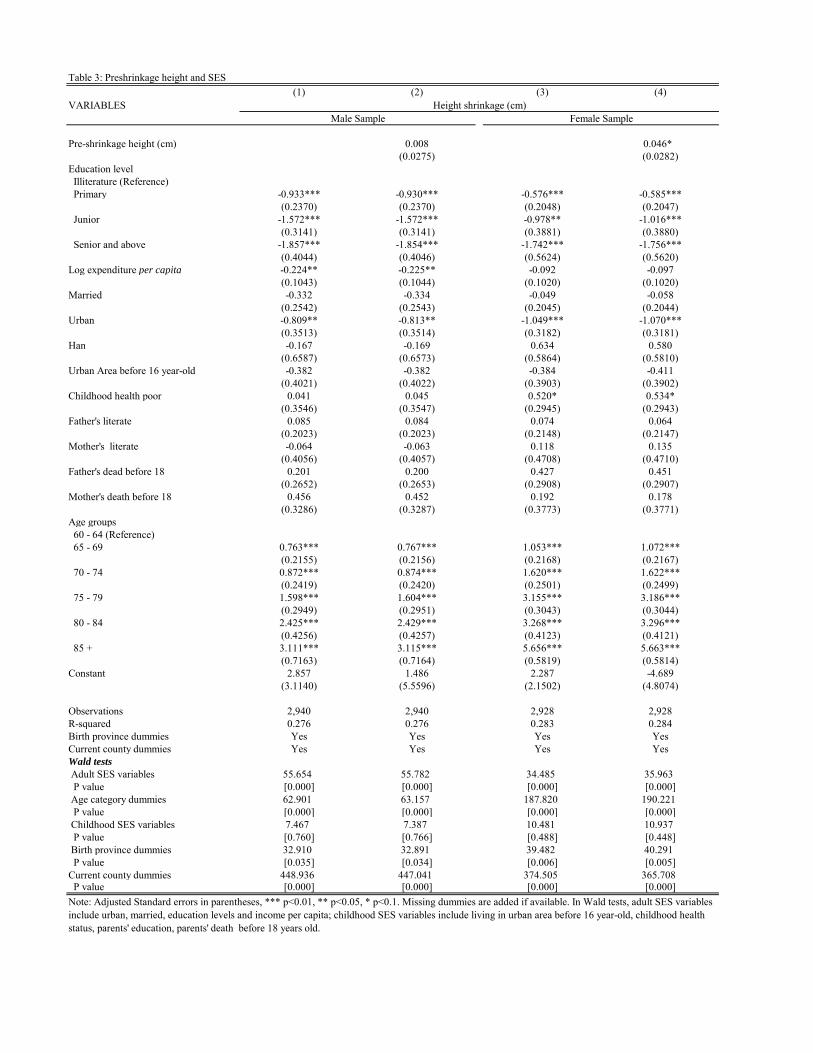
Table 3: Preshrinkage height and SES(1) (2) (3) (4)

VARIABLES

Pre-shrinkage height (cm) 0.008 0.046*(0.0275) (0.0282)

Education level Illiterature (Reference) Primary -0.933*** -0.930*** -0.576*** -0.585***

(0.2370) (0.2370) (0.2048) (0.2047) Junior -1.572*** -1.572*** -0.978** -1.016***

(0.3141) (0.3141) (0.3881) (0.3880) Senior and above -1.857*** -1.854*** -1.742*** -1.756***

(0.4044) (0.4046) (0.5624) (0.5620)Log expenditure per capita -0.224** -0.225** -0.092 -0.097

(0.1043) (0.1044) (0.1020) (0.1020)Married -0.332 -0.334 -0.049 -0.058

(0.2542) (0.2543) (0.2045) (0.2044)Urban -0.809** -0.813** -1.049*** -1.070***

(0.3513) (0.3514) (0.3182) (0.3181)Han -0.167 -0.169 0.634 0.580

(0.6587) (0.6573) (0.5864) (0.5810)Urban Area before 16 year-old -0.382 -0.382 -0.384 -0.411

(0.4021) (0.4022) (0.3903) (0.3902)Childhood health poor 0.041 0.045 0.520* 0.534*

(0.3546) (0.3547) (0.2945) (0.2943)Father's literate 0.085 0.084 0.074 0.064

(0.2023) (0.2023) (0.2148) (0.2147)Mother's literate -0.064 -0.063 0.118 0.135

(0.4056) (0.4057) (0.4708) (0.4710)Father's dead before 18 0.201 0.200 0.427 0.451

(0.2652) (0.2653) (0.2908) (0.2907)Mother's death before 18 0.456 0.452 0.192 0.178

(0.3286) (0.3287) (0.3773) (0.3771)Age groups 60 - 64 (Reference) 65 - 69 0.763*** 0.767*** 1.053*** 1.072*** (0.2155) (0.2156) (0.2168) (0.2167) 70 - 74 0.872*** 0.874*** 1.620*** 1.622***

(0.2419) (0.2420) (0.2501) (0.2499) 75 - 79 1.598*** 1.604*** 3.155*** 3.186***

(0.2949) (0.2951) (0.3043) (0.3044) 80 - 84 2.425*** 2.429*** 3.268*** 3.296***

(0.4256) (0.4257) (0.4123) (0.4121) 85 + 3.111*** 3.115*** 5.656*** 5.663***

(0.7163) (0.7164) (0.5819) (0.5814)Constant 2.857 1.486 2.287 -4.689

(3.1140) (5.5596) (2.1502) (4.8074)

Observations 2,940 2,940 2,928 2,928R-squared 0.276 0.276 0.283 0.284Birth province dummies Yes Yes Yes YesCurrent county dummies Yes Yes Yes YesWald tests Adult SES variables 55.654 55.782 34.485 35.963 P value [0.000] [0.000] [0.000] [0.000] Age category dummies 62.901 63.157 187.820 190.221 P value [0.000] [0.000] [0.000] [0.000] Childhood SES variables 7.467 7.387 10.481 10.937 P value [0.760] [0.766] [0.488] [0.448] Birth province dummies 32.910 32.891 39.482 40.291 P value [0.035] [0.034] [0.006] [0.005]Current county dummies 448.936 447.041 374.505 365.708 P value [0.000] [0.000] [0.000] [0.000]

Height shrinkage (cm)Male Sample Female Sample

Note: Adjusted Standard errors in parentheses, *** p<0.01, ** p<0.05, * p<0.1. Missing dummies are added if available. In Wald tests, adult SES variablesinclude urban, married, education levels and income per capita; childhood SES variables include living in urban area before 16 year-old, childhood healthstatus, parents' education, parents' death before 18 years old.

Table 4.1: Height Shrinkage, Pre-shrinkage Height and Cognitive Abilities(1) (2) (3) (4) (5) (6) (7) (8) (9)

Dependent variablePanel A: Male Sample Measured height 0.0360*** 0.0182*** 0.0050***

(0.00690) (0.00491) (0.00132)Pre-shrinkage height 0.0309*** 0.0313*** 0.0106 0.0109 0.0019 0.0020

(0.00845) (0.00842) (0.00625) (0.00624) (0.00158) (0.00158)Height shrinkage -0.0400*** -0.0244*** -0.0074***

(0.00793) (0.00593) (0.00148)Obeservations 2,927 2,927 2,927 2,707 2,707 2,707 2,927 2,927 2,927R-square 0.308 0.304 0.308 0.187 0.183 0.187 0.199 0.195 0.200Wald tests Adult SES variables 807.481 753.868 332.988 301.605 497.610 457.611 P value [0.000] [0.000] [0.000] [0.000] [0.000] [0.000] Age category dummies 93.486 80.272 168.372 145.235 60.546 48.286 P value [0.000] [0.000] [0.000] [0.000] [0.000] [0.000] Childhood SES variables 60.839 61.088 39.145 38.810 27.090 26.919 P value [0.000] [0.000] [0.000] [0.000] [0.004] [0.004] Birth province dummies 23.453 21.744 27.866 26.266 11.643 10.173 P value [0.267] [0.354] [0.112] [0.156] [0.928] [0.964] Current county dummies 298.559 287.286 325.121 322.363 379.441 376.435 P value [0.000] [0.000] [0.000] [0.000] [0.000] [0.000]

Panel B: Female sample Measured height 0.0446*** 0.0143*** 0.0046***

(0.00807) (0.00542) (0.00135)Pre-shrinkage height 0.0382*** 0.0403*** 0.0092 0.0100 0.0052** 0.0054***

(0.00952) (0.00949) (0.00664) (0.00665) (0.00164) (0.00164)Height shrinkage -0.0477*** -0.0174** -0.0040**

(0.0086) (0.00597) (0.00147)Obeservations 2,907 2,907 2,907 2,612 2,612 2,612 2,907 2,907 2,907R-square 0.332 0.327 0.332 0.208 0.206 0.208 0.223 0.221 0.223Wald tests Adult SES variables 1025.139 965.837 369.093 347.462 652.094 617.288 P value [0.000] [0.000] [0.000] [0.000] [0.000] [0.000] Age category dummies 131.381 96.672 165.509 135.017 61.789 43.737 P value [0.000] [0.000] [0.000] [0.000] [0.000] [0.000] Childhood SES variables 53.047 53.702 40.338 40.371 30.436 30.403 P value [0.000] [0.000] [0.000] [0.000] [0.001] [0.001] Birth province dummies 42.458 40.754 34.007 32.854 42.207 39.123 P value [0.003] [0.004] [0.026] [0.035] [0.003] [0.006] Current county dummies 389.944 384.706 439.203 437.663 481.308 472.446 P value [0.000] [0.000] [0.000] [0.000] [0.000] [0.000]County dummies Yes Yes Yes Yes Yes Yes Yes Yes Yes

Draw a picture ( 0 - 1)TICS (0 - 10) Words recall ( 0 - 10)

Notes: Data source is CHARLS 2011. In Columns (1), (4) and (7), OLS robust standard errors are in parenthesis. In other columns, adjusted standard errors are in parenthesis. All regressions include adult SES variables, age categorydummies, childhood SES variables, birth province dummies and current county dummies. Missing dummies are added, if available. In Wald tests, adult SES variables include urban, married, education levels and log expenditure percapita; childhood SES variables include living in urban area before 16 year-old, childhood health status, parents' education, parents' death before 18 years old.

Table 4.2: Height Shrinkage, Pre-shrinkage Height and Biomarkers(1) (2) (3) (4) (5) (6) (7) (8) (9) (10) (11) (12) (13) (14) (15)

Dependent variablePanel A: Male Sample Measured height 0.0007 2.7220*** 0.3593*** -0.0010 -0.0138**

(0.00156) (0.31405) (0.02342) (0.00134) (0.00581)Pre-shrinkage height -0.0009 -0.0009 2.3068*** 2.3666*** 0.3452*** 0.3498*** -0.0014 -0.0014 -0.0117 -0.0118

(0.00191) (0.00191) (0.4111) (0.40480) (0.03240) (0.03096) (0.00160) (0.00156) (0.00853) (0.00852)Height shrinkage -0.0021 -3.0116*** -0.3673*** 0.0006 0.0155*

(0.00180) (0.37891) (0.02932) (0.00149) (0.00789)Obeservations 2,927 2,927 2,927 2,786 2,786 2,786 2,890 2,890 2,890 2,839 2,839 2,839 2,771 2,771 2,771R-square 0.034 0.034 0.034 0.175 0.159 0.175 0.261 0.224 0.261 0.047 0.046 0.047 0.094 0.092 0.094Wald tests Adult SES variables 28.211 28.218 100.576 73.626 164.605 111.211 23.403 23.129 35.421 32.186 P value [0.000] [0.000] [0.000] [0.000] [0.000] [0.000] [0.001] [0.001] [0.000] [0.000] Age category dummies 94.192 92.443 437.784 367.951 690.391 554.353 93.132 89.712 114.049 105.402 P value [0.000] [0.000] [0.000] [0.000] [0.000] [0.000] [0.000] [0.000] [0.000] [0.000] Childhood SES variables 20.520 20.604 32.773 31.860 21.884 20.854 36.836 36.760 4.850 4.596 P value [0.039] [0.038] [0.001] [0.001] [0.025] [0.035] [0.000] [0.000] [0.938] [0.949] Birth province dummies 23.612 23.492 58.801 61.726 60.492 63.626 19.647 19.536 27.330 27.181 P value [0.251] [0.265] [0.000] [0.000] [0.000] [0.000] [0.480] [0.487] [0.126] [0.130] Current county dummies 222.455 222.168 710.432 742.012 664.279 745.753 320.599 319.910 930.769 935.045 P value [0.000] [0.000] [0.000] [0.000] [0.000] [0.000] [0.000] [0.000] [0.000] [0.000]

Panel B: Female sample Measured height -0.0005 1.7259*** 0.2211*** -0.0010 -0.0152*

(0.00163) (0.23309) (0.02030) (0.00163) (0.00818)Pre-shrinkage height 0.0012 0.0011 1.7805*** 1.8680*** 0.2483*** 0.2570*** -0.0013 -0.0013 -0.0189 -0.0193

(0.00192) (0.00192) (0.28813) (0.28583) (0.02581) (0.02503) (0.00182) (0.00183) (0.01235) (0.01235)Height shrinkage 0.0016 -1.6173*** -0.1954*** 0.0007 0.0122

(0.00173) (0.26376) (0.02253) (0.00167) (0.01063)Obeservations 2,914 2,914 2,914 2,666 2,666 2,666 2,840 2,840 2,840 2,762 2,762 2,762 2,706 2,706 2,706R-square 0.045 0.045 0.045 0.153 0.143 0.153 0.184 0.168 0.185 0.054 0.054 0.054 0.106 0.105 0.106Wald tests Adult SES variables 43.108 41.406 115.130 95.203 151.373 113.936 30.134 28.395 14.680 13.618 P value [0.000] [0.000] [0.000] [0.000] [0.000] [0.000] [0.000] [0.000] [0.023] [0.034] Age category dummies 135.474 116.997 275.751 202.839 377.125 248.273 127.133 115.106 154.043 139.200 P value [0.000] [0.000] [0.000] [0.000] [0.000] [0.000] [0.000] [0.000] [0.000] [0.000] Childhood SES variables 19.210 18.656 14.270 13.348 23.499 23.302 10.471 10.339 19.098 19.327 P value [0.057] [0.067] [0.218] [0.271] [0.015] [0.016] [0.488] [0.500] [0.056] [0.055] Birth province dummies 47.046 47.545 63.897 57.061 123.892 133.308 20.951 21.240 28.443 28.809 P value [0.001] [0.000] [0.000] [0.000] [0.000] [0.000] [0.400] [0.383] [0.099] [0.092] Current county dummies 221.102 222.364 1256.872 1277.526 1193.134 1275.274 354.754 355.244 706.968 706.783 P value [0.000] [0.000] [0.000] [0.000] [0.000] [0.000] [0.000] [0.000] [0.000] [0.000]County dummies Yes Yes Yes Yes Yes Yes Yes Yes Yes Yes Yes Yes Yes Yes YesNotes: Data source is CHARLS 2011. In Columns (1), (4), (7),(10) and (13), OLS robust standard errors are in parenthesis. In other columns, adjusted standard errors are in parenthesis. All regressions include adult SES variables, agecategory dummies, childhood SES variables, birth province dummies and current county dummies. Missing dummies are added, if available. In Wald tests, adult SES variables include urban, married, education levels and log expenditureper capita; childhood SES variables include living in urban area before 16 year-old, childhood health status, parents' education, parents' death before 18 years old.

Walk timeHypertension Lung capacity Grip strength Balance

Table 4.3: Height shrinkage, Pre-shrinkage height and Health(1) (2) (3) (4) (5) (6) (7) (8) (9) (10) (11) (12) (13) (14) (15) (16) (17) (18)

Dependent variablePanel A: Male Sample Measured height -0.0017 -0.0048 -0.0017 -0.0038 -0.0438** -0.0023

(0.00143) (0.00444) (0.00306) (0.00331) (0.01854) (0.00152)Pre-shrinkage height 0.0010 0.0010 0.0097 0.0095 0.0020 0.0020 -0.0006 -0.0007 -0.0305 -0.0314 -0.0005 -0.0006

(0.00170) (0.00170) (0.00508) (0.00508) (0.00342) (0.00343) (0.00369) (0.00369) (0.02282) (0.02280) (0.00182) (0.00182)Height shrinkage 0.0039** 0.0168*** 0.0047 0.0064 0.0541** 0.0037*

(0.00160) (0.00481) (0.00321) (0.00347) (0.0215) (0.00172)Obeservations 2,939 2,939 2,939 2,728 2,728 2,728 2,917 2,917 2,917 2,923 2,923 2,923 2,762 2,762 2,762 2,588 2,588 2,588R-square 0.027 0.027 0.028 0.055 0.055 0.058 0.040 0.040 0.040 0.077 0.076 0.077 0.046 0.044 0.046 0.079 0.078 0.079Wald tests Adult SES variables 56.922 50.477 78.071 67.826 26.294 23.093 55.896 51.114 113.863 103.832 44.367 40.439 P value [0.000] [0.000] [0.000] [0.000] [0.000] [0.001] [0.000] [0.000] [0.000] [0.000] [0.000] [0.000] Age category dummies 14.130 10.836 97.058 81.669 93.867 83.285 161.290 149.749 9.389 7.485 104.208 95.039 P value [0.015] [0.054] [0.000] [0.000] [0.000] [0.000] [0.000] [0.000] [0.095] [0.187] [0.000] [0.125] Childhood SES variables 18.690 17.731 9.607 8.830 14.057 14.572 14.298 14.081 12.912 12.397 9.371 9.284 P value [0.067] [0.088] [0.566] [0.638] [0.230] [0.203] [0.217] [0.361] [0.299] [0.609] [0.537] [0.596] Birth province dummies 17.630 18.092 12.175 12.644 15.999 16.141 18.275 18.460 23.351 23.503 26.513 26.756 P value [0.612] [0.581] [0.910] [0.892] [0.717] [0.707] [0.569] [0.311] [0.272] [0.264] [0.151] [0.142] Current county dummies 193.464 191.734 243.237 247.293 205.035 206.660 234.033 236.328 336.551 335.082 281.223 279.643 P value [0.000] [0.000] [0.000] [0.000] [0.000] [0.000] [0.000] [0.000] [0.000] [0.000] [0.000] [0.000]

Panel B: Female sample Measured height 0.0009 -0.0037 -0.0034 -0.0062 -0.0031 -0.0006

(0.00159) (0.00567) (0.00372) (0.00404) (0.02250) (0.00170)Pre-shrinkage height 0.0036 0.0036 0.0145* 0.0137 0.0104* 0.0097* 0.0124** 0.0115* 0.0356 0.0337 0.0036 0.0034

(0.00183) (0.00184) (0.00611) (0.00611) (0.00393) (0.00394) (0.00430) (0.00431) (0.02580) (0.02585) (0.00197) (0.00197)Height shrinkage 0.0010 0.0165** 0.0129*** 0.0190*** 0.0302 0.0035

(0.00165) (0.0056) (0.00354) (0.00386) (0.02351) (0.00177)Obeservations 2,926 2,926 2,926 2,493 2,493 2,493 2,899 2,899 2,899 2,905 2,905 2,905 2,663 2,663 2,663 2,444 2,444 2,444R-square 0.029 0.029 0.030 0.051 0.052 0.054 0.046 0.046 0.049 0.085 0.086 0.090 0.042 0.043 0.043 0.065 0.066 0.067Wald tests Adult SES variables 16.375 14.366 33.936 27.951 28.839 23.587 49.187 38.845 56.350 52.018 21.638 19.225 P value [0.012] [0.026] [0.000] [0.000] [0.000] [0.001] [0.000] [0.000] [0.000] [0.000] [0.001] [0.004] Age category dummies 23.351 18.747 79.741 60.644 95.268 69.816 189.583 142.781 6.744 4.282 82.793 70.197 P value [0.000] [0.002] [0.000] [0.000] [0.000] [0.000] [0.000] [0.000] [0.240] [0.510] [0.000] [0.000] Childhood SES variables 30.597 29.913 42.269 40.246 15.557 14.268 33.087 31.904 31.338 30.454 25.119 24.470 P value [0.001] [0.000] [0.000] [0.000] [0.158] [0.218] [0.001] [0.001] [0.001] [0.001] [0.009] [0.010] Birth province dummies 31.608 31.070 22.829 22.782 18.201 18.355 34.344 32.951 21.942 21.873 30.080 30.350 P value [0.047] [0.054] [0.263] [0.300] [0.570] [0.564] [0.240] [0.341] [0.343] [0.347] [0.068] [0.064] Current county dummies 245.738 246.612 332.429 335.726 321.363 326.842 291.425 300.903 427.584 427.024 291.672 290.681 P value [0.000] [0.000] [0.000] [0.000] [0.000] [0.000] [0.000] [0.000] [0.000] [0.000] [0.000] [0.000]County dummies Yes Yes Yes Yes Yes Yes Yes Yes Yes Yes Yes Yes Yes Yes Yes Yes Yes Yes

Notes: Data source is CHARLS 2011. In Columns (1), (4), (7), (10), (13) and (16), OLS robust standard errors are in parenthesis. In other columns, adjusted standard errors are in parenthesis. All regressions include adult SES variables,age category dummies, childhood SES variables, birth province dummies and current county dummies. Missing dummies are added, if available. In Wald tests, adult SES variables include urban, married, education levels and logexpenditure per capita; childhood SES variables include living in urban area before 16 year-old, childhood health status, parents' education, parents' death before 18 years old.

Life expectation poorPoor health (0-1) ADLs (0 - 6)Physical Function IADLs (0 - 5) CESD (0 - 30)

Appendix Table 1: Height Comparison with CHNS 1991

MH SD # Obs Age in1991 MH SD PH SD # Obs. MH 2011 -

MH 1991PH 2011 - MH

1991Panel A: Male sample

60 165.64 5.67 106 40 164.02 6.58 166.04 5.05 237 -1.62 0.4061 166.71 5.82 84 41 164.84 6.15 166.60 4.52 219 -1.87 -0.1162 165.66 6.39 82 42 162.80 6.28 165.55 3.79 262 -2.86 -0.1163 165.43 5.61 75 43 163.32 6.15 166.13 4.39 210 -2.12 0.7064 164.81 7.26 79 44 163.51 6.60 165.57 4.25 215 -1.29 0.7765 163.76 6.71 98 45 163.29 6.57 165.83 4.35 183 -0.47 2.0766 164.16 6.40 62 46 162.42 6.40 165.39 4.25 150 -1.73 1.2367 163.36 5.88 57 47 161.44 7.16 165.24 5.09 156 -1.92 1.8868 163.94 6.41 59 48 161.74 6.45 165.14 4.04 162 -2.21 1.2069 163.77 6.45 63 49 160.88 6.56 165.43 4.06 142 -2.89 1.67

Panel B: Female sample60 154.60 5.89 104 40 152.75 5.91 154.76 4.24 292 -1.85 0.1661 153.98 5.90 101 41 152.11 6.00 154.32 3.70 249 -1.86 0.3462 154.19 4.96 97 42 152.53 6.18 154.89 3.88 239 -1.67 0.7063 154.03 5.86 89 43 152.12 6.43 155.06 4.40 188 -1.91 1.0364 155.49 6.03 80 44 152.32 5.92 154.86 4.54 221 -3.16 -0.6365 152.16 6.19 86 45 151.03 6.52 154.07 4.17 175 -1.13 1.9066 153.61 5.87 61 46 151.53 6.16 154.40 3.89 152 -2.08 0.7967 153.28 4.55 58 47 150.41 6.37 154.39 4.47 159 -2.87 1.1168 153.49 5.38 69 48 149.11 6.21 153.83 3.66 128 -4.39 0.3469 153.96 6.54 67 49 150.18 5.54 154.05 3.53 129 -3.79 0.08

Note: MH - Measured Height; PH - Pre-shrinkage Height; SD-Standard Deviation. Unit of heights is centimeter.

Age in 2011CHNS 1991 CHARLS 2011 Differences