1

Health care demand elasticities by type of service

Randall P. Ellis, Bruno Martins, and Wenjia Zhu

Boston University Department of Economics

270 Bay State Road Boston, Massachusetts 02215

USA

ellisrp@bu.edu (corresponding author), bmartins@bu.edu, wz97@bu.edu

April 11, 2017

Abstract

We estimate within-year price elasticities of demand for detailed health care services using an instrumental variable strategy, in which individual monthly cost shares are instrumented by employer-year-plan-month average cost shares. A specification using backward myopic prices gives more plausible and stable results than using forward myopic prices. Using 171 million person-months spanning 73 employers from 2008-2014, we estimate that the overall demand elasticity by backward myopic consumers is -0.44, with high elasticities of demand for pharmaceuticals (-0.44), specialists visits (-0.32), MRIs (-0.29) and mental health/substance abuse (-0.26), and lower elasticities for prevention visits (-0.02), and emergency rooms (-0.04). Demand response is lower for children, in larger firms, among hourly waged employees, and for sicker people. Overall the method appears promising for estimating elasticities for highly disaggregated services although the approach does not work well on services that are very expensive or persistent.

Keywords: Elasticity; cost sharing; high deductible health plans; dynamic demand for health care; myopic expectations.

(JEL: I11, C21, D12)

Acknowledgements: Research for this paper was supported by the National Institute of Mental Health (R01 MH094290). The views expressed here are the authors’ own and not necessarily those of the NIMH. We are grateful to Zarek Brot-Goldberg, Tom McGuire and attendees at the University of Chicago (Will Manning Memorial Conference), Boston University, the University of Oxford, and the American Society of Health Economists for comments on previous versions.

   

2

1. Introduction

This paper revisits the classic issue of price elasticities of demand for health care services, a

topic of central importance for understanding moral hazard and optimal insurance plan design, as

well as having important implications for health plan choice, access to care, health care cost

containment, risk adjustment, and financial risk. Moreover, since modern insurance plans

incorporate highly specific benefit plan features in their designs, and these features can be

customized for demographic, employment, or geographically-defined groups, understanding

demand responses for disaggregated service types is of significant policy interest. In this paper

we use a novel instrumental variable technique on a very large sample (171 million person-

months) to generate estimates of short-run price elasticities of demand among the privately

insured for both aggregated and disaggregated types of services and population subgroups. Many

of our elasticities, particularly for services that are not widely used (e.g., MRIs, mental

health/substance abuse treatment, lab tests, and ambulance use), are infeasible to estimate on

small or modest size samples.

A notable challenge when estimating price elasticities of demand for health care is to control

for endogeneity of prices stemming from endogenous health plan choice. Several estimation

strategies have been used in previous studies to overcome this difficulty, including randomized

control trials (RCTs) (Manning et al. 1987), natural experiments (Duarte 2012; Brot-Goldberg et

al. 2015), and instrumental variable strategies (Eichner 1998; Einav et al. 2015; Kowalski 2016;

Scoggins and Weinberg 2016). Manning et al. (1987) estimated health care demand responses

using RCT data from the RAND Health Insurance Experiment (HIE) conducted in the mid-

1970s, with path-breaking results, but the HIE sample size of 6000 individuals limits its ability to

generate estimates of demand response other than for broad categories of services and large

subpopulations.

Since RCTs such as the HIE are expensive and rare, many studies have exploited natural

experiments that induce changes in prices to estimate demand responsiveness. Duarte (2012) is a

good recent example: he uses Chilean data with a large number of diverse health plans to study

the demand response of both elective (home visits, psychologist visits, physical therapy

evaluations) and acute (appendectomy, cholecystectomy, arm cast) health care services when

government mandates forced employers to increase their coverage generosity. In the similar

spirit, Brot-Goldberg et al. (2015) exploit a natural experiment in health insurance coverage

3

when one large company forced all of its employees to switch to a high-deductible plan. They

find a considerable demand response, even among sick people who expect to exceed deductibles

and face low end-of-year prices, suggesting that many people are myopic, responding strongly to

the spot prices at the time of care is received, and not only the more theoretically correct

expected end-of-year price.

A final approach for estimating unbiased elasticities is to use instrumental variables to

control for the endogeneity of prices (cost shares) within a given year. Eichner (1998) proposes a

novel instrument for within-year price variation: the occurrence of accidental injuries (e.g., a

broken leg) by dependents as an exogenous event that changes subsequent cost sharing and

hence affects the employee’s own demand for medical care. Building on the Eichner framework,

Kowalski (2016) uses emergency department spending for injuries by other family members in

households with at least four members for her estimation of demand responsiveness, where the

instrument (whether a family member incurs spending for an injury) derives its power from the

fact that the event increases the likelihood that the family deductible or stop loss can be

exceeded, thus reducing the marginal price of care faced by the remaining household members.

Einav et al. (2015) use government changes in the Medicare Part D coverage for prescription

drugs as an instrument to study consumer responses to cost sharing, while Scoggins and

Weinberg (2016) use the plan characteristics as an instrument for the actual observed cost share

in claims data. In each case the instrument is based on information that is arguably exogenous to

the individual’s own health expenditure experience.

The two main contributions of this paper are its use of a readily-available and powerful new

instrument, and its use of extremely large data. In our sample, each person contributes twelve

monthly observations on endogenous cost sharing and spending decisions. We include person-

year fixed effects to absorb all aspects of the employer, health plan, locality, supply side prices

and availability, family, and individual patient health and taste variation from estimation, and

then estimate elasticities using monthly data. We also control for seasonality using monthly

dummies. We argue that the remaining variation in individual within-year cost sharing comes

from the nonlinear price schedules in health plans created by deductibles and stoplosses, which

we use to estimate the effects of cost sharing on demand. To control for cost sharing

endogeneity, we use the employer-, year-, and plan-level “leave out one” average monthly cost

share as an instrument for individual cost shares, exploiting the fact that different firms, and

4

different health plans have widely different within-year variation in their cost sharing. We

provide evidence that these employer average cost shares at the plan level have considerable

power and are very weakly correlated with the average health status of plan enrollees.

We estimate elasticities using commercial claims data from 2007-2014 on 171 million

person-months, which allows us to estimate elasticities for very detailed types of health care

services, not usually possible due to the low utilization rates for many such services.

Understanding how consumers react to changes in cost shares for specific services is important

to understand how insurers design their health plans to control for moral hazard and to select

services to offer. In that sense, our paper is similar to Einav et al. (2016), which estimates

demand elasticities for more than 150 pharmaceutical drugs in Medicare Part D.

We are not aware of any other research studies that have used employer-year-plan level

average monthly cost shares to be used as instruments. Our instrument does not rely on any

detailed characteristics of health plans, such as the actual value of deductibles, copayments, and

coinsurance rates, which makes it a useful instrument for large claims data with few employer,

plan, geographic, household, or individual level variables. The method can readily be used to

model spending or utilization at any level of aggregation or subsample including at the level of

individual procedures and drugs.

Let us give a glimpse of our findings before proceeding. We find clear evidence of short run

response to within-year variations in cost sharing: people do respond to within-year price

variation. We explore two types of price expectations, which we call backward myopic and

forward myopic, and argue that they provide upper and lower bounds for the myopic spot prices

consumers seem to use when deciding how much to spend on each type of health care service in

a given month. Our two myopic prices generate demand elasticities that are quite similar for

commonly used services, but backward myopic assumption generates more stable results for

rarely used services. We estimate elasticities of -0.44 for backward myopic expectations versus -

0.41 for forward myopic expectations. This estimate is consistent with the Manning et al (1987)

estimate of -0.2 and the Aron-Dine et al. (2013) reestimation using the HIE data, which is -0.5.

We find heterogeneity in the price elasticity of demand across services, health plans, and

population subgroups. The highest elasticities are for pharmaceuticals (-0.44), specialty visits (-

0.32), and spending on mental health/substance abuse (-0.26), and the lowest elasticities are for

prevention visits (-0.02), emergency rooms (-0.04) and mammogram (-0.11). Supporting Einav

5

et al. (2013), we find evidence of not only biased selection but also heterogeneity in price

responsiveness, with consumers in health plans that have large changes in cost sharing (e.g.,

HDHP) yielding higher estimated demand elasticities than HMOs. Demand elasticities also vary

modestly by enrollee age, risk scores, time, single versus family coverage, salary versus hourly

wage earners, industry, firm size, and firm level average costing.

2. Data

We use IBM/Truven Health MarketScan Commercial Claims and Encounter Database from

2007 to 2014 to identify and extract the claims and enrollment information for all large

employers with at least three years of enrollment information and identifiable plan identifiers.

We checked for but did not find any employers with annual plan enrollment periods other than

the calendar year. We included all individuals, aged 0 to 64, eligible for the full 12 calendar

months of the year, and remaining in the same identified health plan, identified using

MarketScan’s Plankey, a unique health plan identifier. We require at least one month of

eligibility in the year prior to the prediction year, in order to be able to use lagged information

for the evaluation (but not estimation) of our results. We sum up total covered payments and out-

of-pocket (OOP) payments in each calendar month for various types of services. All dollar

amounts were converted into December 2014 dollars by dividing by the appropriate monthly

personal consumption expenditure (PCE) deflator for health care costs from the US Bureau of

Economic Analysis. Monthly spending was also adjusted for the number of days in the month to

remove this minor monthly variation in spending.

For observations in which monthly spending by an individual is positive, we define the cost

share as the ratio between out-of-pocket spending and total spending. Negative or less than $1 of

spending was reset to zero, as likely reflecting payment adjustments, not actual service provision.

Knowing the value of the counterfactual cost share if the individual had positive spending is of

considerable interest for studying the decision to seek care, yet there is little information about

how such expectations are formed. We discuss below our approach for assigning service specific

cost shares (i.e. prices) relevant to consumers for choosing spending levels. We also conduct

sensitivity analysis of dropping plans that rely heavily on copayments rather than cost sharing

since incentives and responsiveness could be quite different in the two.

6

Although the plan type of each health plan is not used in our estimation approach, we use

plan types to evaluate our results. For this study we included only people enrolled in one of the

following six plan types: health maintenance organization (HMO), point of service (POS),

preferred provider organization (PPO), comprehensive (COMP), consumer-directed health plan

(CDHP) and high deductible health plan (HDHP). MarketScan differentiates the CDHP and

HDHP from other plan types not by the size of their deductibles but instead by whether there is a

flexible spending account (CDHP), a health savings account (HDHP), or neither (PPO or POS).

Some PPO or POS plans have high deductibles, while not all CDHP have high cost sharing.

Our final estimation sample used here has data from 73 employers with 732 plans and

information on 14.2 million individual years in six plan types (Table A-1). The mean age is 34.1

years (Table A-2), and average annual total covered spending is $4,648. This large panel enables

us to estimate own-price demand elasticities not only for common, but also for relatively rare

health care services, as well as for various employee and population subgroups. To illustrate our

method, we estimate elasticities for both for broad categories of services (inpatient, outpatient,

and pharmacy) as well as for a variety of non-exhaustive specialized types of service (for

example, ER, chiropractic, MRIs, PET scans, ambulance). Table 1 display summary statistics

for the categories of services modeled here.

3. Methodology

3.1. What prices (or cost shares) matter?

For most goods, a consumer can choose how much to spend without worrying about how

her own spending may change the marginal prices paid. Deductibles, coverage ceilings, and

stoplosses introduce nonlinearities so that the rational consumer looks ahead when making

purchasing decisions. In the path-breaking work by Keeler and colleagues (1988a, 1988b), the

appropriate price for consumers to use is the expected end-of-year price. Ellis (1986) refined this

by modeling how risk-aversion may matter: consumers should optimally make choices using the

end-of-year shadow price, which will be lower for a risk-averse person with a declining block

prices than the expected price. Although it is valuable to have models of the fully rational

consumer, most recent studies, such as by Aron-Dine et al. (2015), Einav et al. (2015), and Brot-

Goldberg et al. (2015), as well as the numerous studies by behavioral economists in other

7

settings, suggest that consumers are considerably more myopic than models of rational consumer

suppose.

In this paper, we focus on short-run demand responses, namely consumer responses to spot

prices captured in the monthly cost shares in each month. Consumer responses to these declining

monthly spot prices during the year can occur for two different reasons. One reason is that

consumers are myopic, and fail to forecast how their current spending affects future prices. The

other, and perhaps more important reason, is that responses to spot prices can reflect perfectly

rational behavior in response to unexpected health shocks that change prices in unanticipated

ways. Although they are conceptually distinct, in this paper we do not distinguish between these

two different mechanisms as they produce observationally equivalent patterns in our data.

Instead, we estimate these short-run responses and summarize them in elasticities, recognizing

that this may underrepresent the long run responsiveness, particularly for foreseeable spending.

To implement our approach, we need a way of calculating the consumer’s spot price, which

we model as a response to a cost share. Given that there is no cost share information for months

in which a consumer did not have any spending, using the actual cost share is not a sufficient

strategy without further assumptions about consumer expectations. Furthermore, our data does

not include general plan parameters, such as copayments and deductibles that would allow us to

predict what the cost share would be in the absence of spending. Some way of reflecting price

expectations is needed to fill in all of the missing prices.

We consider two mechanisms of expectations, which likely provide upper and lower bounds

on the relevant spot prices. For the upper bound, we assume “backward myopic” expectations, in

which a consumer does not know the price until after spending in a month is complete and cost

shares are actually observed (e.g., when the bill is received in the mail). In this case the price

relevant is some previously observed or assumed cost share, which is a backward-looking

framework. We implement this by using the actual monthly cost share for each subsequent

month up until another month with positive spending occurs, after which the backward myopic

cost share is again revised. In this backward-looking framework, it is easy to define prices after a

visit is made, but an initial price is also needed for each consumer before they make a visit,

including those who never make a visit. Here we make the assumption that consumers expect

that the cost share for their first visit will be the average of the health plans cost share for all

other consumers in their first month of seeking care. (If we knew the actual features of our health

8

plans, we might assume that the initial price in a plan with a deductible was one, but our

inference approach leads to nearly that same price.) Specifically, for the backward myopic price,

we assign to individuals the average January cost share of those working for the same employer

and under the same plan in that year.1

The other price expectations process we model is the “forward myopic” consumer. The

forward myopic individual not only knows what the cost sharing will be at the time that services

are chosen in a month, but also uses that price to make decisions prior to that first visit. Hence if

consumer’s first actual visit with a given type of service happens in March, then we use the

actual cost share paid in March for that service as the price for all months January through

March. If the year ends with a span of one or more months with no visits, we continue the cost

share used in the most recent month for the remainder of the year. To complete this model, we

again need to model expectations for consumers who never make a visit. Specifically, we impute

for all months the January average of those within the same employer and plan.

Figure 1 shows a schematic diagram of how prices are assigned for a hypothetical person

who makes visits in March and September in a plan with a deductible and followed by stoploss.

In panel A, the backward myopic individual made no visits in January, and hence is assigned the

average January cost share. The backward myopic consumer uses this same cost share for

February and March. In March, this individual obtains care and pays only 75% of the cost, so

this new lower cost share is used from April through September. Finally, in October, the

consumer observes the 20% cost share from the previous month and adjusts accordingly for the

remaining of the year.

In panel B, the forward myopic consumer fully anticipates the March spending even in

January. From April onwards, the individual expects the cost share to be what it turns out to be

for September, at 20%. Since no further spending occurs for the remainder of the year, this same

rate is also used as the forward myopic price through the end of the year. Although the forward

myopic consumer is more forward looking than the backward myopic consumer, both are

 

1 If no one in a health plan makes a visit for a given service in January, we drop all people in that plan for that year for that service since we cannot impute their backward myopic spot prices. Empirically, this affects only about 0.2% of the sample, mostly for very rarely used services.

9

myopic in that they are not forecasting ahead to the end-of-the-year price and instead are using a

monthly spot price. Nonetheless, these two prices provide upper and lower bounds on the actual

spot prices plausible for each month.

3.2. Estimation equations

We assume health care spending reflects attributes of the individual (i) (which also uniquely

defines a household contract), employer (e), whether the plan is for a family or single coverage

(f), health plan including its own unique provider network (p), geographic location such as the

county or MSA (c), year (y) and a monthly time trend index (t). Using Y for the dependent

variable, and CS* to denote the consumer’s cost share (discussed above) relevant for the choice

of Y, one strategy would be to directly estimate the following.

(1)

For this paper we estimate instead the following much simpler specification.

′ (2)

where ′

This equation estimates the relation between spending and cost share controlling only for

individual-year fixed effects and time trend (year-month) fixed-effects, which has the advantage

of speeding up computation. Since including individual-year fixed effects controls for all of the

individual characteristics that do not vary within the year, we are, in fact, controlling for factors

such as age, gender, risk scores, MSA, plans and any other variables that are fixed within a year.

The monthly time dummies pick up seasonality, changes in national trends, and the effects of

any shocks to the economy (such as recessions). The only covariate over time (in months) is the

individual’s monthly cost share.

We now turn to the issue of functional form, and then instrumental variables.

3.3. Functional form

Our dependent variables in model (2) are characterized by a significant fraction of zero

spending and a long right tail, a well-known feature of health care spending data. To deal with

10

this using annual data, the convention in the literature is to use the log of annual spending plus

one (Aron-Dine et al. 2013, Aron-Dine et al. 2015, Einav et al. 2013, Davis et al. 2016).2 Here

we modified the convention of adding one to accommodate the fact that we are using monthly

rather than annual spending. A priori, we believe using 1/12 makes our results more comparable

to other estimated elasticities modeling annual responsiveness and hence chose that as our base

specification.

For a sensitivity analysis, we estimated models adding an alternative additive constant

within the log specification, a two part model similar to Manning et al (1987) and a specification

using the inverse hyperbolic sine transformation (Burbidge et al, 1988). These results are

discussed in Section 5 and presented in the appendix.

3.4. Instrumental variables

Since cost shares, including our backwards myopic and forward myopic cost shares, reflect

the actual experience of a consumer, they will be endogenous, and using them in OLS for

estimation will lead to biased estimates. For a valid instrument, we need our instrument to be

correlated with this individual price, but uncorrelated with any demand or supply side shocks

that change over time. Note that fixed employer, plan, market or individual characteristics are

absorbed by our individual-year fixed effects, so we are looking for instruments that change

during the twelve calendar months. The previous studies of Eichner (1998) and Kowalski (2016)

used exogenous, individual-level shocks (injuries, and other family member spending decisions)

that are time varying. We use instead the monthly average cost shares for consumers in the same

employer*year*family/single*plan as our instrument. To purge this measure of direct

contamination by a given consumer’s experience, for each person we use the “leave out one”

average, which excludes each person’s own contribution when calculating the average. Hence if

there are N people in a plan for a given month, we use the average of the N-1 other people in that

plan. This measure is exogenous to the individual’s own decisions, but summarizes well the

average time path of cost shares due to deductibles, coinsurance and copayments within a given  

2 The log linear specification has the added advantage of estimating a nonlinear demand curve in which the proportional reduction in demand as the cost share is increased by a fixed amount becomes progressively smaller.

11

plan. F-tests of the power of our instruments in each first stage regression, which correct for

clustered errors, and are discussed in Section 5.

Our IV strategy will lead to unbiased estimates under either of two different assumptions.

One assumption is that all consumers are perfectly backward myopic, never anticipating the

effect of their own spending in the coming month on the cost share, and hence using a backward

view of what the cost share had been in previous months. A second possible condition for

unbiasedness is that there is no biased selection, so the health, the degree of foresight, and the

demand responsiveness mix of people in every plan is identical. In this case the aggregate

average cost share in a plan will also be uncorrelated with errors affecting the individuals own

forward looking behavior.

If people with more foresight or people who are sicker (i.e., have high risk scores) and have

chronic conditions are anticipating lower cost shares as well as clustering in more generous

health plans, then we should see the average aggregate cost share declining with risk scores. The

appendix figure A-1 shows that the average monthly cost sharing is nearly uniformly distributed

across different levels of average risk scores, suggesting our data’s approximation to the second

assumption.

In sum, we estimate IV linear regression models using the two forms of myopic cost shares

as our key variables of interest, while including individual-year and time monthly dummies. We

instrument these cost shares with the employer-year-plan “leave out one” average cost shares for

the corresponding month. Our dependent variable is log(monthly spending plus 1/12), where

1/12 is chosen to make the elasticity estimates correspond to those from annual data models.

Since our model is a log-linear specification, we calculate elasticities from the regression

estimates by multiplying the estimated price coefficient by the average cost share for that

particular service. Errors are corrected for clustering, assumed to be at the level of the employer-

plan-year. Standard errors for the elasticities are generated using the delta method applied to the

least squares standard errors.

4. Results

4.1. Graphical results

Our identification relies on variation across months in average cost shares as well as

variation across health plans in the benefit coverage offered, which are easy to see graphically.

12

Figure 2 shows patterns of average monthly cost shares by plan type. It shows the considerable

variation across months, across plan types, and across broad types of service. There is even more

heterogeneity in our data in that cost shares vary across employers and over time, which is

averaged out in these diagrams. There is also considerable heterogeneity within each single plan

type. High deductible plans have the steepest decline in their average cost shares overall, while

HMOs have cost shares that remain basically constant. CDHPs, comprehensive plans, PPOs, and

POS lie intermediate between the two. Comparing the four panels in the figure, we can see that

outpatient spending shows the steepest decline, closely followed by pharmacy spending.

Inpatient spending shows a relatively modest decline over months, and is particularly flat for

HMOs, as expected since they rely upon supply side controls more than demand side cost

sharing to control costs. One surprise is that HMOs have a nearly constant and relatively high

cost share for pharmacy spending (reflecting a nearly fixed copayment level) and charge a higher

cost share than many other plan types by December.3

If health care spending is responsive to within-year declines in cost sharing, and spot prices

affect spending, then it must be that spending increases during the year. And since cost sharing

declines more in the HDHPs, CDHPs, and PPOs than other plan types, this increase should be

greater for these plan types than for HMOs. We are not aware of any previous study that has

documented this simple prediction. Corresponding to the average cost share by plan in Figure 2A

to 2D, Figure 3A-3D presents average monthly spending in each of our six plan types. Each

diagram pools across all seven years and all the employers, and since we have a balanced sample

with each person in all twelve months for each year in which they are in our analysis, sample

means capture growth in spending over time.

The immediate pattern in all four plots is that costs are generally increasing in all plan types

except for HMOs, where spending per month is nearly flat over time. The lowest line by

December in every figure is the one for the HMOs, which is just below that of HDHPs. The line

for CDHPs more or less follows the pattern of HDHP, low but strongly increasing. At the other

 

3 We speculate, but have not looked into the possibility, that HMOs do a better job at steering their enrollees toward generic drugs, so that even though the cost is lower, the share of drug costs is higher in HMOs than in plans that permit a greater use of branded drugs.

13

extreme, costs are highest for the comprehensive health plan, which does not manage care, and

also has the oldest enrollees and lowest average cost share. PPO spending is generally second

highest, but also growing meaningfully over time.

The remaining panels of Figure 3 illustrate that mean costs are also noticeably increasing for

outpatient spending and pharmaceutical spending. Spending growth is decidedly lower for

inpatient spending, consistent with the slower changing monthly pattern for inpatient cost

sharing, yet an upward trend in HDHP is still evident.

Figure 4 shows empirically the difference in the imputation methodology for three

categories of services and three different plan types – HMO, PPO, and HDHP. HDHPs and

HMOs are on opposite ends of the spectrum of the monthly cost share variation. Indeed, since

the average cost sharing in HMOs is nearly constant from the beginning to the end of the year,

the variation is nearly zero, making the imputations very close to the actual values. In sharp

contrast, HDHPs have sharply declining actual, backwards and forward myopic prices. Both the

backward and forward myopic prices are above the actual values for most of the year. This

reflects the mass of individuals that never make a visit and therefore always have a high price

expectation. This is particularly striking in the case of inpatient spending, where cost share

imputations are nearly constant over time and shows very little variation across the year. The

lack of monthly variation within a plan in inpatient cost sharing is a precursor of why we find it

difficult to estimate the impact of cost share on inpatient categories such as room and board, and

other service categories with precision even in our extremely large sample.

4.2. Regression results

Table 2 presents the IV results from estimating model (2) on overall spending, on three

broad categories of service (outpatient, inpatient, and prescription drugs), and on 22 finer, not

mutually exhaustive, categories of spending, using employer mean cost shares for a month as the

instrument. Separate estimates are presented for backward and forward myopic cost shares

14

models.4 The overall demand elasticity is estimated to be -0.44 using the backward myopic cost

share expectations and -0.41 for forward myopic cost share expectations, which are plausible and

consistent with much of the previous literature.5

The next three rows of Table 2 show heterogeneity between outpatient, inpatient and

pharmacy claims. Our model estimates nearly identical elasticities of -0.29 (backward myopic)

and -0.28 (forward myopic) models. Pharmacy is more elastic, at -0.44 (backward myopic) and -

0.51 (forward myopic). Einav et al. (2016) estimate a mean drug elasticity of -0.24 for a

Medicare Part D, a population older than our sample.6 Inpatient spending is estimated to have a

statistically significant elasticity of -0.30 using the backward myopic price versus an implausible

-2.35 for the forward myopic price. This instability is a symptom of almost all of estimates of

elasticities for relatively rare, inpatient-based services: elasticities are often implausibly large and

generally imprecise. As previously pointed out, we believe this occurs because our IV approach

fails to find a meaningful within-year variation in prices for these services, which happens

invariably when mean monthly spending on a category is high and almost invariably puts a

person over their deductible and stoploss. This is a particular problem for the forward myopic

prices, so for the most part we focus on the backward myopic results in the remainder of this

section.

The remaining rows of Table 2 illustrate elasticities for various services of interest.

Emergency room (ER) spending has an extremely low elasticity of -0.04 using backward myopic

prices, as does maternity (-0.09), consistent with our expectations. Demand response for mental

health and substance abuse (MH/SA) services are of intermediate elasticities (-0.26). This may

 

4 We conducted F-tests of the significant of our first stage instruments, and the minimum F-statistic was 14.65 in the backward myopic specification and 9.03 in the forward myopic specification, with most values greater than 50. Results are presented in table A-3. 

5 Kowalski (2016) uses a different IV approach to estimate the overall demand elasticity of -1.49 at the median percentile.

6 They also estimate an overall drug elasticity of -0.037. However, this elasticity is defined as the probability of filling a claim for any drug, while ours is defined in terms of spending, which also reflects substitution effects between drugs. For this reason, our estimates are more comparable to their mean drug elasticity, which allows for substitution.

15

reflect the current trend that most people getting professional mental health treatment are getting

drugs only or receiving MH/SA treatment in primary care (McGuire, 2016), which is consistent

with the low level of spending on specialty mental health care observed in our data. Surgical

procedures and Dialysis, two very expensive types of services, are of the wrong sign and not

statistically different from zero. Other relatively inelastic services (with backward myopic

elasticities below -0.1) are prevention and ambulance transport.

Although 171 million observations seems like a very large sample, for infrequently used but

expensive services it remains difficult to precisely measure demand response. Table 1 helps

identify the services with very low rates of positive spending but high conditional spending:

home visits, dialysis, and inpatient surgical procedures are examples of this with high standard

errors. Most people with spending on these types of service are likely to be associated with high

annual spending, and thus exceed any reasonable deductible or stoploss, and face very little price

variation. This is also a good argument for why cost sharing on such services will be an

ineffective cost containment tool, since it imposes financial risk with little effect on spending on

these services.

Our methodology may also not be reliable for services that are highly chronic since myopic

spot prices may be less appropriate. Consider drugs, goods, and services such as statins (for high

blood pressure), insulin, oxygen, home health visits for the chronically ill, and long term

behavioral, physical, and occupational therapies. Spending on these services is highly predictable

for many patients, and when expensive, consumers can readily foresee exceeding their

deductibles. Our approach may nonetheless have some power, since even users of these services

may have surprises about other types of spending that affect cost shares. Nonetheless, overall our

approach will be less reliable for persistent types of spending.

5. Extensions and sensitivity analysis

In this section, we re-estimate the model on various partitions of our sample to consider

whether demand response is higher or lower for certain identifiable groups. Since estimated

elasticities are sensitive to the average cost shares in each subgroup, which can vary

dramatically, we present here only the estimates of the demand curve coefficients on all

subgroups, making them comparable. We then conduct a number of sensitivity analyses,

16

examine the robustness of our IVs, and consider alternative functional forms. All of this analysis

focuses on the backward myopic formulation of prices.

5.1. Demand responses by selected subsamples

In this section, we examine price coefficients (not elasticities) of total spending and our

three broad groups of services for various subgroups of our sample. Table 3 presents the results

of our analysis using five different partitions of the individual-years in our estimation sample

using the backward myopic price formulation. In broad terms, our data imply the following

conclusions. Males and females are not statistically significantly different. Spending on children

is less elastic than spending on adults. Pharmacy demand became more elastic from 2008 to

2014. Adults in single versus family contracts are similar in their demand responsiveness, but

children are less price responsive. Enrollees at HMOs are less price responsive than enrollees in

HDHP for outpatient spending but not pharmacy spending. This last finding about pharmacy has

implications for the work of Brot-Goldberg et al. (2015) which focused on changes in demand

from a firm that significantly raised its deductibles, and found relatively large demand

elasticities. This result is also consistent with the results of Einav et al. (2015) who document

heterogeneity in Medicare pharmacy demand.

Table 4 shows the results by various employment-related groups. We find the following.

Enrollees working at a firm in transportation, communications, or utilities have the least price

responsive demand curves. Hourly, non-union employees are less responsive than other salary

classes. Enrollees in low cost sharing firms have more inelastic demand than those in high cost

sharing firms. Demand is less responsive in firms with over 200,000 employees than in firms

with 5,000 to 49,999.

We present this summary of the effects of cost sharing on diverse population and employer

subgroups without attempting to interpret them, primarily as examples of the power of using a

readily available instrument in large samples to explore differences in such dimensions. Studies

using only survey data or a single employer will not have the power to address such refined

issues that may nonetheless be of considerable policy interest.

17

5.2. Robustness of IVs

One concern about our IV is that cost shares are correlated with the degree of consumer

foresight. We therefore generated and examined appendix Figures A-1 for all spending and for

our three broad categories of service. The horizontal axis plots intervals of prospective DxCG

relative risk scores (RRS) for each person based on prior-year diagnostic information. Here the

highest value RRS correspond to being seven times the average spending, while the lowest RRS

interval is .1, which is only 10 percent of the population average. The analysis reveals that as

expected the backwards myopic and forward myopic prices have a sharp downward slope: sicker

people are more likely to exceed any deductibles or stoplosses and pay lower cost shares. But the

modestly downward slope for the employer mean actual cost share suggests that overall there is

only a weak correlation between our instrument and the average health status of enrollees: The

slight downward slope does suggest that enrollees who are sicker tend to work at firms that on

average have more generous coverage, so that their average cost share is slightly lower than the

population average. Ideally there would be no relationship between the “leave out one” mean

cost shares and the RRS. The modest relationship observed implies that our estimated demand

elasticities will be slightly too high rather than too low. We interpret this analysis as saying that

our IV strategy is strong, although not perfect.

5.3. Alternative functional forms

Appendix Table A-5 reports our estimates using the alterative specification of log(Y+1).

Among statistically significant elasticities, using log(Y+1) instead of log(Y+1/12) reduces the

elasticities by 20.8 to 38.1 percent.  

We also estimated results using a two-part model (Manning et al, 1987), in which the first

stage models the binary choice of seeking care and the second stage models the continuous

choice of how much treatment to obtain. Given that we rely on a very large number of

individual-year fixed effects for identification, non-linear models such as logit or selection

models are unattractive or infeasible. Results using a linear probability model are presented in

appendix table A-6. The resulting elasticity estimates are less stable (especially on rarely used

services), which we speculate is because the linear probability model does extremely poorly

when outcome probabilities are very close to zero. The conditional spending results (appendix

18

table A-7) predicting log(spending) are also problematic, with both positive and negative price

effects detected, as can be expected given the large selection effects at the first stage.

In addition to our log linear and two part models, we also estimate results using the inverse

hyperbolic sine function (Burbidge et al, 1988), which provides a different way to accommodate

zero spending together with a thick long tail (Table A-4). We find that results are not very

different from our initial specification and choose to keep the log model as our preferred

specification due to its simplicity.

In sum, we tried three alternative model specifications to our preferred model, and did not

find any of them to be preferable. Clearly, finding better specifications for modeling extremely

skewed data with a preponderance of zeros using fixed effect methods remains an area needing

further research.

6. Conclusions

This paper develops a new IV approach for estimating demand responsiveness using big

data and highly disaggregated types of service. We document and take advantage of the

considerable within-year variation in cost shares in many health plan types, which when

combined with plans that have flat cost sharing creates a nice setting for estimation of demand

elasticities. It seems not to be widely recognized that downward cost sharing trends during the

calendar year must imply upward spending trends on services if there are unexpected spending

shocks, or consumers are myopic. We show that these patterns are strong across many types of

service, showing that within-year price responsiveness is significant. We acknowledge that our

results represent only US employees working at large firms, but our estimates improve on those

coming from only a single large employer. Our results suggest that studies using only a single

employer, or using only people who are in high deductible plans may not generalize since they

are not representative of the full population of privately insured.

Our IV strategy leads to elasticity estimates that are plausible and consistent with other

estimates from the literature for services where a single month of use does not typically put a

person over normal deductible levels. Our IV approach works less well for expensive procedures

like hospice care, inpatient surgery, room and board spending, and dialysis, where the time of the

year matters less since the consumer will almost invariably exceed the deductible. While not

19

perfect, our IV has the advantage of being widely available and easy to use. OLS estimates, in

contrast are often in the wrong sign.

An innovation of the paper is that we estimate two different forms of spot prices: backward

myopic prices where consumers never anticipate future spending, and forward myopic spot

prices, where they fully anticipate actual spending in the current when making consumption

decisions. We find relatively modest differences in our elasticities once we ignore statistically

insignificant ones. One hypothesis for this is that our two measures are highly correlated when

consumers use a service multiple times per year, and since we use an IV strategy, it corrects for

expectation errors.

Our approach holds great promise in potentially providing a new instrument – employer

average monthly cost share on a service of interest – which can be used in other studies looking

for an instrument for rates of spending or utilization of a service. For example, consider

procedure ABC, lab test DEF, or drug GHI that are sometimes used only for a patient with

condition 123. If consumers are diagnosed with condition 123 at different times in the year, and

face changing cost shares over time, then our approach can be used to generate a reasonable

instrument for assessing the effectiveness of each of these procedures, tests, or drugs for treating

condition 123. Given how valuable it is to have good instruments, other uses may prove to be as

useful as the estimates of demand response that we generate here.

20 

References

Aron-Dine, Aviva, Liran Einav, and Amy Finkelstein. 2013. “The RAND Health Insurance

Experiment, Three Decades Later.” Journal of Economic Perspectives, 27(1): 197-222.

Aron-Dine, Aviva, Liran Einav, Amy Finkelstein, and Mark R. Cullen. 2015. “Moral Hazard in

Health Insurance: Do Dynamic Incentives Matter?” The Review of Economics and Statistics,

97(4): 725-741.

Brot-Goldberg, Zarek C., Amitabh Chandra, Benjamin R. Handel, and Jonathan T. Kolstad.

November 2, 2015. “What Does a Deductible Do? The Impact of Cost-Sharing on Health Care

Prices, Quantities, and Spending Dynamics.” Working Paper.

Burbidge, John B., Lonnie Magee, and A. Leslie Robb. 1988. “Alternative Transformations to

Handle Extreme Values of the Dependent Variable.” Journal of the American Statistical

Association, 83(401): 123-127.

Davis, Matthew A., Brahmajee K. Nallamothu, Mousumi Banerjee, and Julie P.W. Bynum. 2016.

“Identification of Four Unique Spending Patterns among Older Adults in the Last Year of Life

Challenges Standard Assumptions.” Health Affairs, 35(7): 1316-1323.

Duarte, Fabian. 2012. “Price Elasticity of Expenditure across Health Care Services.” Journal of

Health Economics, 31(6): 824-841.

Eichner, Matthew J. 1998. “The Demand for Medical Care: What People Pay Does Matter.”

American Economic Review, 88(2): 117-121.

Einav, Liran, Amy Finkelstein, Stephen P. Ryan, Paul Schrimpf, and Mark R. Cullen. 2013.

“Selection on Moral Hazard in Health Insurance.” American Economic Review, 103(1): 178-

219.

Einav, Liran, Amy Finkelstein, and Paul Schrimpf. 2015. “The Response of Drug Expenditure to

Non-Linear Contract Design: Evidence from Medicare Part D.” The Quarterly Journal of

Economics. doi: 10.1093/qje/qjv005

Einav, Liran, Amy Finkelstein, and Maria Polyakova. 2016. “Private Provision of Social

Insurance: Drug-Specific Price Elasticities and Cost Sharing in Medicare Part D.” NBER

Working Paper 22277

Ellis, Randall P. 1986. “Rational Behavior in the Presence of Coverage Ceilings and

Deductibles.” The Rand Journal of Economics, 17(2): 158-175.

21 

Keeler, Emmett B., Willard G. Manning, and Kenneth B. Wells. 1988. “The Demand for

Episodes of Mental Health Services.” Journal of Health Economics, 7(4): 369-392.

Keeler, Emmett B. and John E. Rolph. 1988. “The Demand for Episodes of Treatment in the

Health Insurance Experiment.” Journal of Health Economics, 7(4): 337-367.

Kowalski, Amanda. 2016. “Censored Quantile Instrumental Variable Estimates of the Price

Elasticity of Expenditure on Medical Care.” Journal of Business & Economic Statistics, 34(1):

107-117.

Manning, Willard G, Joseph P. Newhouse, Naihua Duan, Emmett B. Keeler, and Arleen

Leibowitz. 1987. “Health Insurance and the Demand for Medical Care: Evidence from A

Randomized Experiment.” American Economic Review, 77(3): 251-277.

McGuire, Thomas G. 2016. “Achieving Mental Health Care Parity Might Require Changes In

Payments And Competition.” Health Affairs, 35(6): 1029-1035.

Scoggins, John. F. and Daniel A. Weinberg. 2016. “Healthcare Coinsurance Elasticity Coefficient

Estimation Using Monthly Cross-sectional, Time-series Claims Data.” Health Economics, doi:

10.1002/hec.3341. 

22 

Backward myopic uses the prior cost share.

1A

Forward myopic uses the next actual cost share.

1B

Fig. 1. Two models of expectations

Note: Shown are the backward myopic and forward myopic expected cost shares for a single, hypothetical consumer who makes visits only in March and September, and who experiences an average cost share of .75 in March, and .2 in September. The average cost share for a person making their first visit in January for this employer*year*plan is assumed to be .90. The backward myopic consumer uses this price up through March, then lowers expectations after visits are made in March, and again in October. The forward myopic consumer anticipates the cost shares in March and September and uses them until new information comes along.

23 

2A

2B

2C

2D

Fig. 2. Average monthly cost share by plan type, 2008-2014 Note: Each panel plots the average actual cost share for the services indicated by month, averaged over the seven year period for each plan type for the 73 employer sample. People not using a service in the month are excluded.

24 

3A

3B

3C

3D

Fig. 3. Average monthly spending by plan type, 2008-2014 Note: Each panel plots the monthly spending for the services indicated by month, averaged over the seven year period for each plan type for the 73 employer sample. People not using a service in the month are included as zero spending.

25 

4A

4B

4C

4D

Fig. 4. Cost share imputations for HMOs, PPOs and HDHPs by Type of Service Note: Each panel shows the actual, backward myopic, and forward myopic cost shares for three plan types: HMOs, PPOs, and HDHPs. The four panels correspond to All, Outpatient, Inpatient and Pharmacy spending.

26 

Table 1. Monthly summary statistics on the study variables, by Types of Service (TOS)

Type of Service Mean

Monthly Spending

% Total Spending

Std. Dev

Mean cost share (%)

% obs. Positive spending

Mean spending if

positive

All Spending 387 100.00 2,968 31.06 46.35 836 Outpatient 222 57.27 1,397 27.34 32.15 690 Inpatient 80 20.68 2,408 8.62 0.42 19,096 Pharmaceutical 85 22.05 519 40.76 34.24 249 Maternity 12 3.22 433 18.66 0.39 3,232 MH/SA 11 2.84 303 29.77 3.00 366 ER 19 4.97 289 25.09 1.42 1,355 Room and Board 31 8.13 1,497 9.47 0.26 11,920 Non specialty visits 26 6.66 220 28.18 17.14 151 Home visits 1 0.26 108 7.60 0.08 1,219 Prevention 5 1.23 27 4.28 3.48 137 Surgical procedures 8 1.98 538 4.05 0.07 11,554 Surgical supplies/devices 5 1.31 406 4.86 0.06 7,977 Specialty visits 63 16.36 775 30.85 9.58 661 Dialysis 3 0.70 253 4.14 0.03 8,337 PT, OT, speech therapy 9 2.29 114 24.36 2.96 300 Chiropractic 2 0.61 21 37.73 2.49 95 CAT scans 6 1.44 130 18.48 0.60 932 Mammograms 3 0.71 33 6.15 1.13 241 MRIs 7 1.70 123 18.49 0.56 1,176 PET scans 1 0.15 46 7.32 0.02 2,467 Radiology - diagnostic 6 1.65 108 22.70 3.41 188 Ultrasounds 3 0.75 42 22.85 1.12 260 Diagnostic services 11 2.72 236 17.20 2.85 370 DME 2 0.64 89 22.17 0.68 362 Ambulances 2 0.53 165 15.30 0.14 1,464 Note: Table reports summary statistics for the 26 types of services (TOS) identified and constructed from the MarketScan Commercial Claims and Encounter Database. N = 170,963,286 individual months.

27 

Table 2. IV regression results showing demand responses to two types of cost share

Backward myopic cost share Forward myopic cost share

Model: log(1/12 + Y) Coefficient Elasticity S.E Coefficient Elasticity S.E

All Spending -1.26 -0.44 0.044 -1.26 -0.41 0.041Outpatient -0.86 -0.29 0.034 -0.91 -0.28 0.033Inpatient -2.18 -0.30 0.045 -17.37 -2.35 0.357Pharmaceutical -1.00 -0.44 0.040 -1.12 -0.51 0.045Maternity -0.27 -0.09 0.042 -0.39 -0.12 0.060MH/SA -0.62 -0.26 0.046 -0.93 -0.39 0.069ER -0.12 -0.04 0.024 -0.51 -0.17 0.102Room and Board -1.44 -0.20 0.069 -8.18 -1.14 0.389Non specialty visits -0.73 -0.25 0.041 -0.90 -0.28 0.046Home visits -0.06 -0.01 0.071 -0.25 -0.05 0.326Prevention -0.34 -0.02 0.009 -4.86 -0.29 0.123Surgical procedures 1.33 0.07 0.098 28.85 1.52 2.139Surgical supplies/devices -3.13 -0.22 0.090 -80.88 -5.76 2.318Specialty visits -0.80 -0.32 0.033 -1.10 -0.42 0.043Dialysis 0.17 0.02 0.156 0.31 0.04 0.290PT, OT, speech therapy -0.33 -0.15 0.032 -0.60 -0.27 0.057Chiropractic -0.36 -0.23 0.065 -0.47 -0.30 0.083CAT scans -0.49 -0.15 0.023 -2.64 -0.80 0.123Mammograms -1.02 -0.11 0.027 -19.92 -1.97 0.499MRIs -0.95 -0.29 0.022 -7.30 -2.21 0.171PET scans -1.13 -0.17 0.081 -7.35 -1.13 0.528Radiology - diagnostic -0.42 -0.15 0.018 -1.09 -0.38 0.044Ultrasounds -0.38 -0.14 0.015 -1.54 -0.56 0.060Diagnostic services -0.53 -0.15 0.021 -1.54 -0.42 0.059DME -0.39 -0.18 0.038 -1.00 -0.47 0.097Ambulances -0.31 -0.07 0.052 -4.75 -1.00 0.806Note: N = 170,963,286 individual months. Each row is a different regression using the log(spending plus 1/12) as the dependent variable. Each model includes individual*year fixed effects, 12 monthly time dummies and uses employer’s average cost share for that year*plan*family*month, without the own individual, as an instrument. Cluster corrected standard errors use the employer*plan for clusters. Elasticities are evaluated at the mean cost share for that particular type of service, and S.E obtained using the delta method.

28 

Table 3. Estimated demand coefficients by demographic and plan subgroups

Model: log(1/12 + Y), backward myopia expectations, IV results % of sample All spending Outpatient Inpatient Pharmacy Benchmark 100 -1.26 -0.86 -2.18 -1.00Gender Male 48.50 -1.29 -0.83 -1.69 -1.02 Female 51.50 -1.24 -0.88 -2.48 -0.99Age group 0 to 5 6.39 -0.56 -0.25 -2.03 -0.68 6 to 20 23.67 -0.88 -0.41 -1.19 -0.97 21 to 45 34.87 -1.37 -0.91 -2.90 -0.92 46 to 64 35.07 -1.49 -1.14 -1.82 -1.09Plan type HMO 9.97 -1.49 -0.59 0.34 -1.15 PPO 65.51 -1.17 -0.74 -2.59 -0.74 HDHP 1.82 -1.39 -1.34 -3.34 -1.17Time period 2008-2009 30.67 -0.81 -0.52 -1.98 -0.33 2010-2012 49.74 -1.41 -1.08 -1.98 -1.03 2013-2014 19.59 -1.07 -0.70 -1.95 -1.22Plan coverage Single 21.11 -1.47 -1.04 -0.93 -1.13 Family, employee 25.26 -1.61 -1.16 -2.59 -1.08 Family, spouse 19.95 -1.37 -1.01 -2.90 -0.98 Family, child 33.68 -0.83 -0.40 -1.80 -0.89Note: Table shows the unconditional estimated demand coefficients for all services and for three broad types of services by gender, age group, risk score ranges, selected plan types, time interval and plan coverage. Each coefficient is from a different IV regression. Each IV regression includes individual*year fixed effects and 12 monthly time dummies and uses employer's average cost share for that service in that year*plan*family*month as an instrument for the myopic cost share. Dependent variable is log of spending on that service plus one. Cluster corrected standard errors use the employer*plan for clusters.

29 

Table 4. Estimated demand coefficients by employment-related subgroups

Model: log(1/12 + Y), backward myopia expectations, IV results

% of sample All spending Outpatient Inpatient Pharmacy

Benchmark 100 -1.26 -0.86 -2.18 -1.00

Industry

Services 11.94 -1.52 -1.09 -2.80 -1.67

Manufacturing, Durable Goods 14.18 -1.59 -1.27 -1.66 -0.96

Finance, Insurance, Real Estate 12.78 -1.33 -0.89 -1.62 -1.18

Transportation, Communications, Utilities 13.55 -0.35 -0.15 -4.20 -1.16

Salary class

Union (salaried or hourly) 14.44 -1.24 -0.82 -2.13 -0.93

Salaried, non-union 27.19 -1.22 -0.79 -2.32 -0.86

Hourly, non-union 20.11 -0.95 -0.56 -1.89 -1.02

Employers by level of average cost sharing

Lowest quartile 22.84 -1.08 -0.73 -2.53 -0.89

Second quartile 33.90 -1.06 -0.82 -2.48 -0.81

Third quartile 25.34 -1.66 -0.92 -2.29 -0.85

Highest quartile 17.92 -1.38 -1.65 -1.72 -1.10

Employers by number of employees

2,800 to 49,999 20.31 -1.41 -0.97 -2.12 -1.04

50,000 to 199,999 46.91 -1.20 -0.85 -1.90 -0.97

200,000 or more 32.78 -0.87 -0.41 -3.42 -1.22 Note: Table shows the unconditional estimated demand coefficients for all services and for three broad types of services by industry, salary class, and employer quartiles of costs share. For the last group individuals were divided into four quartiles according to a ranking of the average cost share of their employer in that year, such that the lowest quartile are at employers offering the lowest average cost share. Each coefficient in this table comes from a different IV regression. Each IV regression includes individual*year fixed effects, 12 monthly time dummies and uses employer's average cost share for that service in that year*plan*family*month as an instrument. Dependent variable is log of spending on that service plus 1/12. Cluster corrected standard errors use the employer*plan for clusters.

30 

For Online Publication

Appendix Figures and Tables

A B

C D

Fig. A-1. Plot of intervals of risk scores versus monthly cost shares for three price measures, all spending, outpatient services, inpatient services, and pharmacy

Note: Each point in each diagram plots the average cost share for all person-month observations with a risk score in the 0.1 intervals ranging from .1 to 7.0. Three different cost shares are plotted: the backward myopic and forward myopic cost shares, which are the individual level prices, and the average “all but one” employer cost share for a plan month, which is our instrument. The figures illustrate that while both backward myopic and forward myopic prices decline sharply with higher risk scores, employer average costs in a month, which pool people with diverse risks, show very little decrease across risk scores. N=169,452,390.

31 

Table A-1. Plan type market shares in the sample

Year HMO POS PPO Comprehensive CDHP HDHP

2008 13.34 14.97 64.46 1.12 5.97 0.13 2009 19.95 9.10 61.94 2.70 5.02 1.29 2010 12.45 9.53 68.78 1.75 6.11 1.38 2011 10.32 15.54 67.59 1.73 4.52 0.30 2012 11.93 18.66 55.96 1.61 11.69 0.15 2013 13.30 3.59 75.70 0.37 2.12 4.92 2014 6.66 4.28 47.75 2.21 31.47 7.63

All 12.79 11.62 63.47 1.69 8.68 1.76 Note: Table shows plan type market shares overall and by year in the study sample. N = 170,963,286 individual months. HMO=Health Maintenance Organization, POS=Point-of-Service, PPO=Preferred Provider Organization, CDHP=Consumer-Driven Health Plan, HDHP=High Deductible Health Plan.

Table A-2.Characteristics of individuals in the sample

Year Obs. Individuals Age Female Concurrent Risk Score

Prospective Risk Score

2008 26,530,356 2,210,863 34.2 0.52 1.00 0.992009 26,180,802 2,181,734 34.0 0.52 1.11 1.022010 30,290,976 2,524,248 34.4 0.52 1.16 1.102011 29,583,504 2,465,292 34.0 0.51 1.15 1.092012 25,271,124 2,105,927 33.8 0.50 1.14 1.072013 15,744,564 1,312,047 34.6 0.51 1.28 1.102014 17,361,960 1,446,830 34.1 0.50 1.33 1.07ALL 170,963,286 14,246,941 34.1 0.51 1.15 1.06

Note: Table summarizes individual characteristics overall and by year in the study sample. N = 170,963,286 individual months.

32 

Table A-3. First stage F-statistics of IV regressions

Backward myopic cost share Forward myopic cost share

F-statistic F-statistic

All Spending 844.53 1148.97 Outpatient 1895.03 1443.58 Inpatient 283.93 99.31 Pharmaceutical 789.94 1456.37 Maternity 436.3 343.57 MH/SA 571.81 531.55 ER 577.23 206.59 Room and Board 82.35 15.95 Non specialty visits 1109.5 939.05 Home visits 166.73 73.22 Prevention 35.26 32.11 Surgical procedures 35.36 9.03 Surgical supplies/devices 15.38 10.44 Specialty visits 671.16 583.79 Dialysis 50.83 25.1 PT, OT, speech therapy 418.17 434.02 Chiropractic 171.57 202.54 CAT scans 399.74 348.71 Mammograms 14.65 10.17 MRIs 350.88 317.91 PET scans 62.6 38.26 Radiology - diagnostic 600.77 675.64 Ultrasounds 575.52 587.91 Diagnostic services 395.34 443.92 DME 583.39 475.81 Ambulances 128.6 48.18 Note: N = 170,963,286 individual months. Each row is different first stage regression using either the backward myopic cost share or forward myopic cost share as the dependent variable. Each model includes individual*year fixed effects, 12 monthly time dummies and uses employer’s average cost share for that year*plan*family*month, without the own individual, as an instrument. Cluster corrected standard errors use the employer*plan for clusters for the F-statistic calculation. The first stage is independent of the log transformation applied in the second stage.

33 

Table A-4. Sensitivity analysis

Model: log(1/12 + Y), backward myopia expectations, IV results    % of sample All spending Outpatient Inpatient PharmacyBenchmark 100 -1.26 -0.86 -2.18 -1.00

Inverse hyperbolic sine transformation 100 -1.03 -0.68 -1.85 -0.82

Plans with less than 50% of out-of-pocket in copays 66.88 -1.21 -0.83 -2.00 -0.96

Dropped January and December 83.29 -1.23 -0.85 -3.11 -0.84Risk score groups 0.0 to 0.99 68.44 -1.23 -0.75 -0.11 -0.88 1.0 to 1.99 18.67 -1.36 -1.07 -0.57 -1.06 2.0 to 3.99 9.57 -1.20 -1.00 -2.48 -1.13 4 or more 3.32 -1.01 -0.80 -1.40 -1.13Note: N = 170,963,286 individual months. Each row is a different regression using the log(spending plus 1/12) as the dependent variable. Each model includes individual*year fixed effects, 12 monthly time dummies and uses employer’s average cost share for that year*plan*family*month, without the own individual, as an instrument. Cluster corrected standard errors use the employer*plan for clusters.

34 

Table A-5. Robustness check using log(spending+1) as the dependent variable

Backward myopic cost share Forward myopic cost share

Model: log(1 + Y) Coefficient Elasticity S.E Coefficient Elasticity S.E

All Spending -0.94 -0.33 0.031 -0.94 -0.31 0.029Outpatient -0.61 -0.21 0.024 -0.64 -0.20 0.023Inpatient -1.73 -0.24 0.035 -13.75 -1.86 0.280Pharmaceutical -0.74 -0.33 0.026 -0.83 -0.38 0.030Maternity -0.20 -0.06 0.031 -0.29 -0.09 0.044MH/SA -0.42 -0.18 0.031 -0.64 -0.27 0.047ER -0.09 -0.03 0.017 -0.37 -0.12 0.074Room and Board -1.09 -0.15 0.053 -6.19 -0.86 0.301Non specialty visits -0.45 -0.16 0.025 -0.56 -0.17 0.028Home visits -0.01 0.00 0.050 -0.07 -0.01 0.231Prevention -0.22 -0.01 0.006 -3.20 -0.19 0.083Surgical procedures 1.05 0.06 0.077 22.89 1.21 1.672Surgical supplies/devices -2.48 -0.18 0.070 -64.10 -4.56 1.806Specialty visits -0.56 -0.22 0.022 -0.77 -0.29 0.029Dialysis 0.12 0.02 0.123 0.22 0.03 0.228PT, OT, speech therapy -0.23 -0.10 0.021 -0.41 -0.19 0.038Chiropractic -0.24 -0.15 0.042 -0.31 -0.19 0.054CAT scans -0.34 -0.11 0.016 -1.87 -0.57 0.088Mammograms -0.70 -0.07 0.018 -13.59 -1.34 0.338MRIs -0.69 -0.21 0.016 -5.33 -1.62 0.125PET scans -0.86 -0.13 0.061 -5.59 -0.86 0.398Radiology - diagnostic -0.28 -0.10 0.011 -0.72 -0.25 0.029Ultrasounds -0.26 -0.09 0.010 -1.04 -0.38 0.041Diagnostic services -0.35 -0.10 0.013 -1.04 -0.28 0.037DME -0.27 -0.13 0.025 -0.69 -0.32 0.064Ambulances -0.22 -0.05 0.039 -3.40 -0.72 0.591Note: N = 170,963,286 individual months. Each row is a different regression using the log(spending plus 1) as the dependent variable. Each model includes individual*year fixed effects, 12 monthly time dummies and uses employer’s average cost share for that year*plan*family*month, without the own individual, as an instrument. Cluster corrected standard errors use the employer*plan for clusters. Elasticities are evaluated at the mean cost share for that particular type of service, and S.E obtained using the delta method.

35 

Table A-6. Two-part model – Visit binary choice

Backward myopic cost share Forward myopic cost share

Model: 1(Y > 0) Coefficient S.E. Elasticity Coefficient S.E. Elasticity

All Spending -0.13 0.016 -0.10 -0.13 0.0155 -0.09Outpatient -0.10 0.013 -0.11 -0.11 0.0137 -0.10Inpatient -0.18 0.029 -5.95 -1.46 0.2289 -47.08Pharmaceutical -0.10 0.013 -0.13 -0.11 0.0148 -0.15Maternity -0.03 0.014 -2.34 -0.04 0.0208 -3.37MH/SA -0.08 0.014 -1.10 -0.12 0.0215 -1.65ER -0.01 0.008 -0.31 -0.06 0.0346 -1.32Room and Board -0.14 0.046 -7.49 -0.80 0.2579 -42.33Non specialty visits -0.11 0.020 -0.23 -0.14 0.0241 -0.25Home visits -0.02 0.039 -4.27 -0.08 0.1818 -19.62Prevention -0.05 0.019 -0.08 -0.67 0.2775 -1.14Surgical procedures 0.11 0.165 8.83 2.41 3.5799 191.81Surgical supplies/devices -0.26 0.115 -29.30 -6.74 2.9685 -756.51Specialty visits -0.10 0.011 -0.41 -0.13 0.0151 -0.53Dialysis 0.02 0.101 8.97 0.04 0.1871 16.65PT, OT, speech therapy -0.04 0.009 -0.65 -0.08 0.0173 -1.17Chiropractic -0.05 0.015 -1.30 -0.07 0.0192 -1.68CAT scans -0.06 0.009 -2.92 -0.31 0.0464 -15.71Mammograms -0.13 0.034 -1.19 -2.56 0.6601 -22.29MRIs -0.10 0.008 -5.64 -0.79 0.0614 -42.94PET scans -0.11 0.053 -72.25 -0.71 0.3445 -469.93Radiology - diagnostic -0.06 0.007 -0.62 -0.15 0.0179 -1.55Ultrasounds -0.05 0.005 -1.63 -0.20 0.0221 -6.48Diagnostic services -0.07 0.011 -0.70 -0.21 0.0332 -1.97DME -0.05 0.011 -3.34 -0.13 0.0290 -8.62Ambulances -0.04 0.027 -5.35 -0.54 0.4123 -82.16Note: N = 170,963,286 individual months. Each row is a different regression using the 1(spending > 0) as the dependent variable. Each model includes individual*year fixed effects, 12 monthly time dummies and uses employer’s average cost share for that year*plan*family*month, without the own individual, as an instrument. Cluster corrected standard errors use the employer*plan for clusters. Elasticities are evaluated at the mean cost share and fraction of enrollees with a positive visit for that particular type of service.

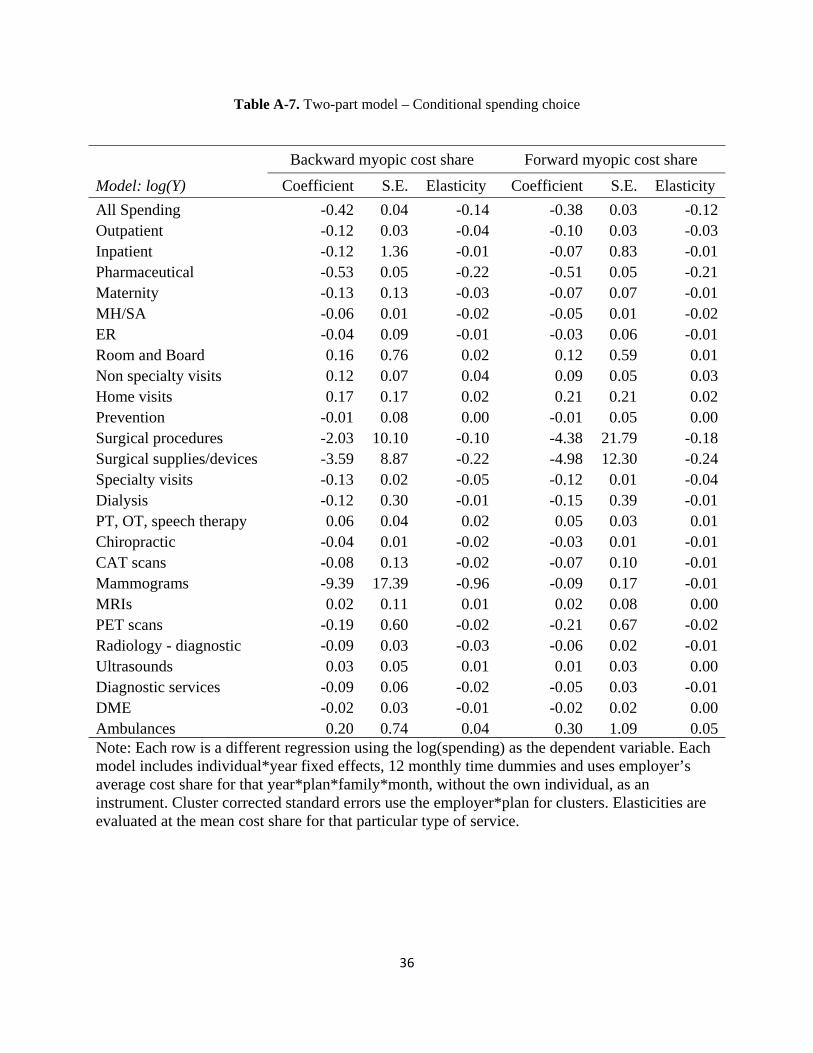
36 

Table A-7. Two-part model – Conditional spending choice

Backward myopic cost share Forward myopic cost share

Model: log(Y) Coefficient S.E. Elasticity Coefficient S.E. Elasticity

All Spending -0.42 0.04 -0.14 -0.38 0.03 -0.12Outpatient -0.12 0.03 -0.04 -0.10 0.03 -0.03Inpatient -0.12 1.36 -0.01 -0.07 0.83 -0.01Pharmaceutical -0.53 0.05 -0.22 -0.51 0.05 -0.21Maternity -0.13 0.13 -0.03 -0.07 0.07 -0.01MH/SA -0.06 0.01 -0.02 -0.05 0.01 -0.02ER -0.04 0.09 -0.01 -0.03 0.06 -0.01Room and Board 0.16 0.76 0.02 0.12 0.59 0.01Non specialty visits 0.12 0.07 0.04 0.09 0.05 0.03Home visits 0.17 0.17 0.02 0.21 0.21 0.02Prevention -0.01 0.08 0.00 -0.01 0.05 0.00Surgical procedures -2.03 10.10 -0.10 -4.38 21.79 -0.18Surgical supplies/devices -3.59 8.87 -0.22 -4.98 12.30 -0.24Specialty visits -0.13 0.02 -0.05 -0.12 0.01 -0.04Dialysis -0.12 0.30 -0.01 -0.15 0.39 -0.01PT, OT, speech therapy 0.06 0.04 0.02 0.05 0.03 0.01Chiropractic -0.04 0.01 -0.02 -0.03 0.01 -0.01CAT scans -0.08 0.13 -0.02 -0.07 0.10 -0.01Mammograms -9.39 17.39 -0.96 -0.09 0.17 -0.01MRIs 0.02 0.11 0.01 0.02 0.08 0.00PET scans -0.19 0.60 -0.02 -0.21 0.67 -0.02Radiology - diagnostic -0.09 0.03 -0.03 -0.06 0.02 -0.01Ultrasounds 0.03 0.05 0.01 0.01 0.03 0.00Diagnostic services -0.09 0.06 -0.02 -0.05 0.03 -0.01DME -0.02 0.03 -0.01 -0.02 0.02 0.00Ambulances 0.20 0.74 0.04 0.30 1.09 0.05Note: Each row is a different regression using the log(spending) as the dependent variable. Each model includes individual*year fixed effects, 12 monthly time dummies and uses employer’s average cost share for that year*plan*family*month, without the own individual, as an instrument. Cluster corrected standard errors use the employer*plan for clusters. Elasticities are evaluated at the mean cost share for that particular type of service.