Header Space Analysis: Static Checking For NetworksPeyman KazemianStanford University

kazemian@stanford.edu

George VargheseUCSD and Yahoo Labsvarghese@cs.ucsd.edu

Nick McKeownStanford University

nickm@stanford.edu

Abstract

Today’s networks typically carry or deploy dozensof protocols and mechanisms simultaneously such asMPLS, NAT, ACLs and route redistribution. Even whenindividual protocols function correctly, failures can arisefrom the complex interactions of their aggregate, requir-ing network administrators to be masters of detail. Ourgoal is to automatically find an important class of fail-ures, regardless of the protocols running, for both opera-tional and experimental networks.

To this end we developed a general and protocol-agnostic framework, called Header Space Analysis(HSA). Our formalism allows us to statically check net-work specifications and configurations to identify an im-portant class of failures such as Reachability Failures,Forwarding Loops and Traffic Isolation and Leakageproblems. In HSA, protocol header fields are not firstclass entities; instead we look at the entire packet headeras a concatenation of bits without any associated mean-ing. Each packet is a point in the {0, 1}L space where Lis the maximum length of a packet header, and network-ing boxes transform packets from one point in the spaceto another point or set of points (multicast).

We created a library of tools, called Hassel, to imple-ment our framework, and used it to analyze a variety ofnetworks and protocols. Hassel was used to analyze theStanford University backbone network, and found all theforwarding loops in less than 10 minutes, and verifiedreachability constraints between two subnets in 13 sec-onds. It also found a large and complex loop in an exper-imental loose source routing protocol in 4 minutes.

1 Introduction“Accidents will occur in the best-regulatedfamilies” — Charles Dickens

In the beginning, a switch or router was breathtak-ingly simple. About all the device needed to do was in-dex into a forwarding table using a destination address,and decide where to send the packet next. Over time,forwarding grew more complicated. Middleboxes (e.g.,NAT and firewalls) and encapsulation mechanisms (e.g.,VLAN and MPLS) appeared to escape from IP’s lim-itations: e.g., NAT bypasses address limits and MPLS

allows flexible routing. Further, new protocols for spe-cific domains, such as data centers, WANs and wireless,have greatly increased the complexity of packet forward-ing. Today, there are over 6,000 Internet RFCs and it isnot unusual for a switch or router to handle ten or moreencapsulation formats simultaneously.

This complexity makes it daunting to operate a largenetwork today. Network operators require great sophisti-cation to master the complexity of many interacting pro-tocols and middleboxes. The future is not any more rosy- complexity today makes operators wary of trying newprotocols, even if they are available, for fear of break-ing their network. Complexity also makes networks frag-ile, and susceptible to problems where hosts become iso-lated and unable to communicate. Debugging reacha-bility problems is very time consuming. Even simplequestions are hard to answer, such as “Can Host A talkto Host B?” or “Can packets loop in my network?” or“Can User A listen to communications between UsersB and C?”. These questions are especially hard to an-swer in networks carrying multiple encapsulations andcontaining boxes that filter packets.

Thus, our first goal is to help system administratorsstatically analyze production networks today. We de-scribe new methods and tools to provide formal answersto these questions, and many other failure conditions, re-gardless of the protocols running in the network.

Our second goal is to make it easier for system ad-ministrators to guarantee isolation between sets of hosts,users or traffic. Partitioning networks this way is usuallycalled “slicing”; VLANs are a simple example used to-day. If configured correctly, we can be confident that traf-fic in one slice (e.g. a VLAN) cannot leak into another.This is useful for security, and to help answer questionssuch as “Can I prevent Host A from talking to Host B?”.For example, imagine two health-care providers usingthe same physical network. HIPAA [20] rules requirethat no information about a patient can be read by otherproviders. Thus a natural application of slicing is to placeeach provider in a separate slice and guarantee that nopacket from one slice can be controlled by or read by theother slice. We call this secure slicing. Secure slicingmay also be useful for banks as part of defense-in-depth,and for classified and unclassified users sharing the samephysical network. Our tools can verify that slices have

been correctly configured.Our third goal is to take the notion of isolation fur-

ther, and enable the static analysis of networks sliced inmore general ways. For example, with FlowVisor [6] aslice can be defined by any combination of header fields.A slice consists of a topology of switches and links, theset of headers on each link, and its share of link capac-ity. Each slice has its own control plane, allowing itsowner to decide how packets are routed and processed.While tools such as FlowVisor allow rapid deployment ofnew protocols, they add to the complexity of the network,pushing the level of detail beyond the comprehension ofa human operator. Our tools allow automatic analysis ofthe network configuration to formally prove that the slic-ing is operating as intended.

In the face of this need, it is surprising that there arevery few existing network management tools to analyzelarge networks. Further, the tools that exist are proto-col dependent and specialized to each task. For example,the pioneering work of Xie, et al [4] on static reachabil-ity analysis, the analyses of IP connectivity and firewallconfiguration, e.g. [9, 10, 11, 15], and work on routingfailures [12, 13] are all tailored to IP networks. Whilethese papers suggest powerful approaches for reachabil-ity in IP networks, they do not easily extend to new pro-tocols and new types of checks.

This paper introduces a general framework, calledHeader Space Analysis, which provides a set of toolsand insights to model and check networks for a varietyof failure conditions in a protocol-independent way. Keyto our approach is a generalization of the geometric ap-proach to packet classification pioneered by Lakshmanand Stiliadis [3], in which classification rules over Kpacket fields are viewed as subspaces in aK dimensionalspace.

We generalize in three ways. First, we jettison the no-tion of pre-specified fields in favor of a header space ofL bits where each packet is represented by a point in{0, 1}L space, where L is the header length. This al-lows us to work with emerging protocols and arbitraryfield formats. Second, we go beyond modeling packetclassification in which a header is mapped to a singlepoint in a matching subspace. Instead, we model allrouter and middlebox processing as box transfer func-tions transforming subspaces of the L-dimensional spaceto other subspaces. For example, in Figure 1, A and Bare arbitrary boxes, and TA and TB represent their trans-fer functions. We model how a packet or flow is modifiedas it travels by composing the transfer functions alongthe path. Third, we go beyond modeling a single box tomodeling a network of boxes using a network transferfunction, Ψ and a topology transfer function, Γ. Ψ com-bines all individual box functions into one giant function.Γ models the links that connect ports together. The over-

A B

TA() TB()

a b

A B

TB(TA())

a b Tab()

(a)

(b)

Figure 1: (a) Changes to a flow as it passes through two boxes withtransfer function TA and TB . (b) Composing transfer functions tomodel end to end behavior of a network.

all behavior of the network is modeled as a black box bycomposing Ψ and Γ along all paths.

The contributions of this paper and an outline of therest of the paper are as follows:

• Header Space Analysis: Section 2 describes the ge-ometric model and defines transfer functions. Sec-tion 3 shows how transfer functions can be usedto model today’s networking boxes. Section 4 de-scribes an algebra for working on header space.• Use Cases: Section 5 describes how header space

analysis can be used to detect network failures suchas reachability failures, routing loops and slice iso-lation in a protocol independent way.• Implementation: Section 6 describes a library of

tools (called Hassel, or Header Space Library),based on header space analysis, that can staticallyanalyze networks. We describe five key optimiza-tions that boost Hassel’s performance by 5 ordersof magnitude relative to a naive implementation.• Experiments: Section 7 reports results of using Has-

sel to analyze three examples: (1) Stanford Univer-sity’s backbone network, (2) Slice isolation check,and (3) An experimental source routing protocol.We report loops found, and show that even ourPython implementation scales to large enterprisenetworks with our optimizations.

We describe limitations of our approach and relatedwork in Sections 8 and 9. We conclude in Section 10.

2 The Geometric ModelOur header space framework is built on a geometricmodel. We model packets as points in a geometric spaceand network boxes as transfer functions on the same ge-ometric space. Our first task is to define the main geo-

2

metric spaces.Header Space, H: We ignore the protocol-specific

meanings associated with header bits and view a packetheader as a flat sequence of ones and zeros. Formally,a header is a point and a flow is a region in the {0, 1}Lspace, where L is an upper bound on the header length.We call this space Header Space,H.

A wildcard expression is the basic building block usedto define objects in H. Each wildcard expression is asequence of L bits where each bit can be either 0, 1 or x.Each wildcard expression corresponds to a hypercube inH. Every region, or flow, in H is defined as a union ofwildcard expressions.H abstracts away the data portion of a packet because

we assume it does not affect packet processing. If itdoes, as in an intrusion-detection box, then L must bethe length of the entire packet. If the fields are fixed, wecan define macros for each field in H to reduce dimen-sionality. However, the general notion of header space iscritical when dealing with different protocols that inter-pret the same header bits in different ways. Note also thatwe can model variable length fields such as IP optionsusing a custom parsing function as shown in Section 7.3.

Network Space, N : We model the network as a setof boxes called switches with external interfaces calledports each of which is modeled as having a unique iden-tifier. We use “switches” to denote routers, bridges, andany possible middlebox.

If we take the cross-product of the switch-port space(the space of all ports in the network, S) with H, wecan represent a packet traversing on a link as a point in{0, 1}L × {1, ..., P} space, where {1, ..., P} is the listof ports in the network. We call the space of all possiblepacket headers, localized at all possible input ports in thenetwork, the Network Space, N .

Network Transfer Function, Ψ(): As a packet tra-verses the network, it is transformed from one pointin Network Space to other point(s) in Network Space.For example, a layer 2 switch, that merely forwards apacket from one port to another, without rewriting head-ers, transforms packets only along the switch-port axis,S. On the other hand, an IPv4 router that rewrites somefields (e.g. MAC address, TTL, checksum) and then for-wards the packet, transforms the packet both in H andS.

As these examples suggest, all networking boxes canbe modeled as Transformers with a Transfer Function(see Figure 1), that models their protocol dependentfunctions. More precisely, a node can be modeled us-ing its transfer function, T , that maps header h arrivingon port p:

T (h, p) : (h, p)→ {(h1, p1), (h2, p2), ...}In general, the transfer function may depend on the input

port to model input-port-specific behavior and the outputmay be a set of (header, port) pairs to allow multicast-ing.1

A concept we use heavily is the network transferfunction, Ψ(.). Given that switch ports are numbereduniquely, we combine all the box transfer functions intoa composite transfer function describing the overall be-havior of the network. Formally, if a network consists ofn boxes with transfer functions T1(.), ..., Tn(.), then:

Ψ(h, p) =

T1(h, p) if p ∈ switch1

... ...

Tn(h, p) if p ∈ switchn

Topology Transfer Function, Γ(): We can modelthe network topology using a topology transfer function,Γ(), defined as:

Γ(h, p) =

{{(h, p∗)} if p connected to p∗

{} if p is not connected.

Γ models the behavior of links in the network. It acceptsa packet at one end of a link and returns the same packet,unchanged, at the other end. Note that links are unidi-rectional in this model. To model bidirectional links, onerule should be added per direction.

Multihop Packet Traversal: Using the two transferfunctions, we can model a packet as it traverses the net-work by applying Φ(.) = Ψ(Γ(.)) at each hop. For ex-ample, if a packet with header h enters a network on portp, the header after k hops will be Ψ(Γ(...(Ψ(Γ(h, p)...),or simply Φk(h, p): each Γ forwards the packet on a linkand each Ψ passes the packet through a box.

Slice: A slice, S, can be defined as (Slice networkspace, Permission, Slice Transfer Function) where Slicenetwork space is a subset of the network space controlledby the slice, and Permission is a subset of {read(r),write(w)}2. The Slice Transfer Function, Ψs(h, p), cap-tures the behavior of all rules installed by the controlplane of slice S. For example, a slice that controls pack-ets destined to subnet 192.168.1.0/24 and is restricted tonetwork ports 1, 2 and 3 can be expressed as ((ip dst(h)= 192.168.1.x , p ∈ {1, 2, 3}), rw , Ψs). Here, ip dst(h)is a helper function refering to the IP destination bits inthe header.

Our concept of a slice combines two notions we nor-mally think of as very different. It describes the implicitslicing, when protocols coexist today on the same net-work using protocol IDs (e.g. TCP and UDP) or net-works partitioned using Vlan IDs. It also describes the

1It also enables us to model load balancing boxes for which theoutput port is a psuedo-random function of the header bits.

2A real slice may have other attributes such as bandwidth reserva-tions, but our model ignores attributes irrelevant to the analysis.

3

explicit slicing utilized by FlowVisor [6] to create in-dependent experiments in an OpenFlow [5] network, asdone in testbed networks such as GENI3 [19].

3 Modeling Networking BoxesThis section is a brief tutorial on transfer functions in or-der to illustrate their power in modeling different boxesin a unified way. We use helper functions for clarity.We refer to a particular field in a particular protocolusing helper function protocol field(). For example,ip src(h) refers to the source IP address bits of headerh. Similarly, helper function R(h, fields, values) isused to rewrite the fields in h with values. For exam-ple, R(h,mac dst(), d) rewrites the MAC destinationaddress to d. Header updates can be represented by amasking AND followed by a rewrite OR.

We start by modeling an IPv4 router which processespackets as follows: 1) Rewrite source and destinationMAC addresses, 2) Decrement TTL, 3) Update check-sum, 4) Forward to outgoing port. Thus the transfer func-tion of an IPv4 router concatenates four functions:

TIPv4(.) = Tfwd(Tchksum(Tttl(Tmac(.)))).

We examine each function in turn. Tfwd(.) looks upip dst(h) in a lookup table and returns the output port.If lookup is modeled as ip lookup(.) : ip dst→ port:

Tfwd(h, p) = {(h, ip lookup(ip dst(h)))}

Similarly, Tmac(.) looks up the next hop MAC addressand updates source and destination MAC addresses.Tttl(.) drops the packet if ip ttl(h) is 0 and otherwisedoes R(h, ip ttl(), ip ttl(h) − 1). Tchksum(.) updatesthe IP checksum. If the focus is on IP routing, wemight choose to ignore Tmac(.), simplifying the modelto TIPv4(.) = Tfwd(Tttl(.)) or even TIPv4(.) = Tfwd().As an example, a simplified transfer function of an IPv4router that forwards subnet S1 traffic to port p1, S2 trafficto port p2 and S3 traffic to port p3 is:

Tr(h, p) =

{(h, p1)} if ip dst(h) ∈ S1

{(h, p2)} if ip dst(h) ∈ S2

{(h, p3)} if ip dst(h) ∈ S3

{} otherwise.

A firewall is modeled as a transfer function that ex-tracts IP and TCP headers, matches the headers againsta sequence of wildcard expressions (which model ACLrules), and drops or forwards the packet as specified bythe matching rule. A tunneling end point is modeled us-ing a shift operator that shifts the payload packet to theright and a rewrite operator that rewrites the beginning

3In GENI parlance, the network space of a slice is called flow space.

of the header. A Network Address Translator (NAT) boxcan also be modeled using a rewrite operator. Howeverthe level of details that we use in our model depends onthe application. For example we can have a detailedmodel where we model the exact source IP to sourcetransport port mapping, or we may set the output trans-port source port to a wildcard (all x) to represent everypossible mapping. In [1] we provide more examples.While modeling is trivial but tedious, we have writtentools that parse router configuration files and forwardingtables to automate the process.

4 Header Space AlgebraAlgorithms that compute reachability or determine if twoslices can interact must determine how different spacesoverlap. We therefore need to define basic set operationson H: intersection, union, complementation and differ-ence. We also define the Domain, Range and Range In-verse for transfer functions. The next section shows howthis algebra is used.

4.1 Set Operations onHWhile set operations on bit vectors are well-known, weneed set operations on wildcard expressions. Since allobjects in header space can be represented as a unionof wildcard expressions, defining set operation on wild-card expressions allows these operations to carry overto header space objects. For the rest of this paper, weoverload the term header to refer to both packet headers(points in H) and wildcard expressions (hyper-cubes inH).

Intersection: For two headers to have a non-emptyintersection, both headers must have the same bit valueat every position that is not a wildcard. If two headersdiffer in bit bi, then the two headers will be in differenthyper-planes defined by bi = 0 and bi = 1. On the otherhand, if one header has an x in a position while the otherheader has a 1 or 0, the intersection is non-empty. Thus,the single-bit intersection rule for bi ∩ b′i is defined as:

HHHHHbi

b′i 0 1 x

0 0 z 01 z 1 1x 0 1 x

In the table, z means the bitwise intersection is empty.The intersection of two headers is found by applying thesingle-bit intersection rule, bit-by-bit, to the headers. z isan “annihilator”: if any bit returns z, the intersection ofall bits is empty. As an example, 11000xxx ∩ xx00010x= 1100010x and 1100xxxx ∩ 111001xx = 11z001xx = φ.A simple trick allows efficient software implementation.

4

Encode each bit in the header using two bits: 0 → 01,1 → 10, x → 11 and z → 00. Intersection, then, issimply an AND operation on the encoded headers.

Union: In general, a union of wildcard expressionscannot be simplified. For example, no single headercan represent the union of 1111xxxx and 0000xxxx.This is why a header space object is defined as a unionof wildcard expressions. In some cases, we can sim-plify the union (e.g., 1100xxxx ∪ 1000xxxx simplifiesto 1x00xxxx) by simplifying an equivalent boolean ex-pression. For example, 10xx ∪ 011x is equivalent tob4b3 ⊕ b4b3b2. This allows the use of Karnaugh Mapsand Quine-McCluskey [18] algorithms for logic mini-mization.

Complementation: The complement of header h —the union of all headers that do not intersect with h — iscomputed as follows:h′ ← φfor bit bi in h do

if bi 6= x thenh′ ← h′ ∪ x...xbix...x

end ifend forreturn h′

The algorithm finds all non-intersecting headers by re-placing each 0 or 1 in the header with its complement.This follows because just one non-intersecting bit (orz) in a term results in a disjoint header. For example,(100xxxxx)′ = 0xxxxxxx ∪ x1xxxxxx ∪ xx1xxxxx.

Difference: The difference (or minus) operation canbe calculated using intersection and complementation.A−B = A ∩B′. For example:

100xxxxx− 10011xxx =100xxxxx ∩ (0xxxxxxx ∪ x1xxxxxx ∪ xx1xxxxx∪xxx0xxxx ∪ xxxx0xxx)= φ ∪ φ ∪ φ ∪ 1000xxxx ∪ 100x0xxx= 1000xxxx ∪ 100x0xxx.

The difference operation can be used to check if oneheader is a subset of another: A ⊆ B ⇐⇒ A−B = φ.

4.2 Domain, Range and Range InverseTo capture the destiny of packets through a box or set ofboxes, we define the domain, range and range inverse asfollows:

Domain: The domain of a transfer function is the setof all possible (header, port) pairs that the transfer func-tion accepts. Even headers for which the output is empty(i.e., dropped packets) belong to the domain.

Range: The range of a transfer function is the set of allpossible (header, port) pairs that the transfer function canoutput after applying all possible inputs on every port.

Range Inverse: Reachability and loop detection com-putation requires working backwards from a range todetermine what input (header, port) pairs could haveproduced it. If S = {(h1, p1), ..., (hj , p2)}, thenthe range inverse of S under transfer function T (.) isX = {(hi, pi)}]n1 such that T (X) = S. Equivalently,X = T−1(S). The inverse of a transfer function is well-defined: A transfer function maps each (h, p) pair to aset of other pairs. By following the mapping backward,we can invert a transfer function.

5 Using Header Space AnalysisIn this section we show how the header space analy-sis – developed in the last three sections – can be usedfor solving several classical networking problems in aprotocol-agnostic way.

5.1 Reachability AnalysisXie, et. al. [4] analyze reachability by tracing which ofall possible packet headers at a source can reach a des-tination. We follow a similar approach, but generalizeto arbitrary protocols. Using header space analysis, weconsider the space of all headers leaving the source, thentrack this space as it is transformed by each successivenetworking box along the path (or paths) to the destina-tion. At the destination, if no header space remains, thetwo hosts cannot communicate. Otherwise, we trace theremained header spaces backwards (using the range in-verse at each step) to find the set of headers the sourcecan send to reach the destination.

Consider, for example, the question: Can packets fromhost a reach host b?. Define the reachability function Rbetween a and b as:

Ra→b =⋃

a→b paths

{Tn(Γ(Tn−1(......(Γ(T1(h, p)...))}

where for each path between a and b, {T1, ..., Tn−1, Tn}are the transfer functions along the path. The switches ineach path are denoted by:

a→ S1 → ...→ Sn−1 → Sn → b.

The Range of Ra→b is the set of headers that can reachb from a. Notice that these headers are seen at b, andnot necessarily headers transmitted by a, since headersmay change in transit. We can find which packet headerscan leave a and reach b by computing the range inverse.If header h ⊂ H reached b along the a → S1 → ...→ Sn−1 → Sn → b path, then the original header sentby a is:

ha = T−11 (Γ(...(T−1

n−1(Γ(T−1n ((h, b))...)),

using the fact that Γ = Γ−1.

5

a

A0

A1

B0

B1

1001xxxx 0011xxxx

xxxxxxxx

1001xx10 0011xx10

C0

D0

10011x10

C1 C2

E1

10010x10

01011x10

E0 D1

b

01011x10

10010x10

E2

C3

TD(h, p) =

8>>><>>>:

if h=100xxxxx, p = D0 :{((h&00011111)|01000000, D1)}if h=110xxxxx, p = D1 :{((h&00011111)|01100000, D0)}

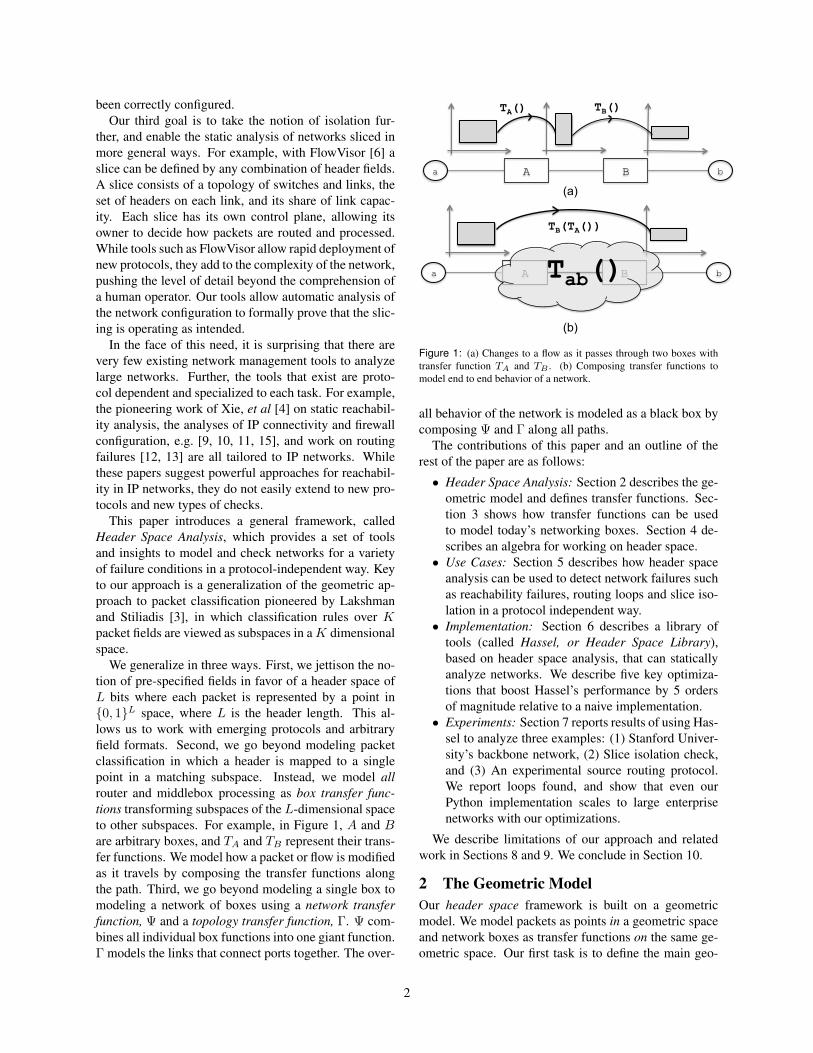
Figure 2: Example for computing reachability function from a to b. For simplicity, we assume a header length of 8 and show the first 4 bits on thex-axis and the last 4 bits on the y-axis. We show the range (output) of each transfer function composition along the paths that connect a to b. At theend, the packet headers that b will see from a are 01011x10 ∪ 10010x10.

To provide intuition, we do reachability analysis forthe small example network in Figure 2. Each box in Fig-ure 2 contains its transfer function. To keep things sim-ple, we only use 8-bit headers; since we cannot easilydepict eight dimensions, we represent the first 4 bits ofthe header on the x-axis and the last 4 bits on the y-axis.Note that in this example, A and C are miniature modelsof IP routers, B is a firewall, D is a simplified NAT boxand E behaves like an Ethernet switch.

Figure 2 shows how the network boxes transformheader space along each path. By repeatedly applyingthe output of each transfer function to the input of thenext transfer function in each path, the reachability func-tion from a to b becomes:

Ra→b(h, p) =

if h=10010x10, p = A0 :{(h,E2)}if h=10011x10, p = A0 :{((h&00011111)|01000000, E2)}

The range ofRa→b, which is the final output set in Figure2, is 10010x10 ∪ 01011x10. This is the set of headersthat can reach b from a. To find the set of headers thata can send to b, we compute the range inverse of Ra→b

which is 10010x10 ∪ 10011x10.Complexity: As we push the test packet toward the

destination, the transfer function rules divide the inputheaderspace into smaller pieces. If the headerspace con-sists of the union of R1 wildcard expressions and thetransfer function has R2 rules, then the output can be aheaderspace with O(R1R2) wildcard expressions. How-ever, this is the worst case scenario. In a real network

whose purpose is to provide connectivity, as the headerspace propagates to the core of the network, the matchpatterns of forwarding rules will become less specific,therefore the space will not be divided into too manypieces. Most of the flow division happens as a resultof rules that are filtering out some part of input flow(e.g. ACL rules). As a result, each of the input wildcardexpressions will match only a few rules in the transferfunction and generate at most cR (and not R2), wherec << R. We call this, the Linear Fragmentation as-sumption. Under this assumption, the running time isO(dR2) where d is the network diameter – the maxi-mum number of hubs that a packet will go through beforereaching the destination – andR is the maximum numberof forwarding rules in a router. See [1] for more details.While our algorithm may appear almost to be a simula-tion, we gain algorithmic leverage by treating groups ofheaders as an equivalence class wherever possible. Bycontrast, a brute-force algorithm that simulates the send-ing of every possible packet has O(2L) complexity.

5.2 Loop DetectionA loop occurs when a packet returns to a port it hasvisited earlier. Header space analysis can determine allpacket headers that loop. We first describe how to detectgeneric loops and then show how to detect infinite loops,a subset of generic loops where packets loop indefinitely.An example of a generic, but finite loop, is an IP packetthat loops until the TTL decrements to zero.Generic Loops: Given a network transfer function, wedetect all loops by injecting an all-x test packet header(i.e., a packet header, all of whose bits are wild-carded)

6

TA()

TC()

TB()

TD()

hret

A

C

B

D

a b

C0 C1

A2

A0

A1

D1 D0

B2

B1 B0

all-x

C2

D2

b0 a0

horig

TD-1()

TB-1()

TC-1()

TA-1()

Figure 3: An example network for running the loop detection algo-rithm. The solid lines show the changes in the all-x test packet injectedfrom A1 till it returns to the injection port as hret. The dashed linesshow the process of detecting infinite loop, where hret is traced backto find horig , the part of all-x packet that caused hret.

Hdr:All-x Port: A1 Visits: -

Hdr:H1 Port: a0

Visits: A1

Hdr:H2 Port: C0

Visits: A1

Hdr:H3 Port: B1

Visits: C0,A1

Hdr:H4 Port: D2

Visits: C0,A1

Hdr:H7 Port: B2

Visits:D2,C0,A1

Hdr:H9 Port: b0

Visits:B2,D2,C0,A1

Hdr:H6 Port: b0

Visits:B1,C0,A1

Loop!

Hdr:H5 Port: D0

Visits:B1,C0,A1

Hdr:H8 Port: A1

Visits:D0,B1,C0,A1

Figure 4: Example of the propagation graph for a test packet injectedfrom port A1 in network of figure 3.

from each port in the network and track the packet until:

• (Case 1) It leaves the network;• (Case 2) It returns to a port already visited (Pret);

or• (Case 3) It returns to the port4 it was injected from

(Pinj).

Only in Case 3 – i.e. the packet comes back to its in-jection port — do we report a loop. Since we repeat thesame procedure starting at every port, we will detect thesame loop when we inject a test packet from Pret. Ignor-ing Case 2 avoids reporting the same loop twice.

We find loops using breadth first search on the prop-agation graph. For example, in Figure 3 we inject theall-x test packet into port A1. Figure 4 is the correspond-ing propagation graph. Each node in the propagation

4While we could define a loop as a packet returning to a node visitedearlier, using ports helps detect infinite loops.

graph shows the set of packet headers, Hdr, that reacheda Port and the set of ports visited previously in theirpath: Visits. For example, in Figure 4:

{(H3, B1), (H4, D2)} = Φ(H2, C0).

We detect a loop when Port is the first element ofVisits. 5

The generic loop detection test has the same algorith-mic structure as reachability test, and hence its complex-ity is similarly O(dPR2) under the Linear Fragmenta-tion assumption. Here P is number of ports that we needto inject the test packet from. See [1] for more details.Finding Single Infinite Loops: Not all generic loopsare infinite. For example, in the loop “A → C → B →D → A” in Figure 3, the header space changes as thetest packet traverses the loop. Let hret denote the part ofheader space that returns to A1. Then horig, defined as

horig = Φ−1(Φ−1(Φ−1(Φ−1(hret, A1))))

is the original header space that produces hret. Figure 3also depicts the process of finding horig.

Now, hret and horig relate in one of three ways:1. hret ∩ horig = φ: In this case, the loop is surely

finite. The header space that caused the loop, i.e. horig,does not intersect with the returned header space, and theloop will terminate.

2. hret ⊆ horig: in this case the loop is certainlyinfinite. Every packet header in horig is mapped by thetransfer function of the loop to a point in hret. Since hret

is completely within horig, the process will repeat in thenext round, and the loop will continue indefinitely.

3. Neither of the above: In this case, we need to iterateagain. First, note that hret − horig completely satisfiesCase 1’s condition, and therefore cannot loop again. Butwe must examine hret ∩ horig. So we redefine hret :=hret ∩horig and calculate the new horig. We repeat untilone of the first two cases happens. The process mustterminate (in at most 2L steps) because at each step thenewly defined hret shrinks. Hence, eventually case 1 or2 will happen, or hret will be empty.6

More tortuous loops, where a packet passes throughother loops before coming back to a first loop, can alsobe detected using a simple generalization [1].

5.3 Slice IsolationNetwork operators often wish to control which groupsof hosts (or users) can communicate with each other.

5If Port appears anywhere else in Visits, we terminate thebranch.

6IP TTL is an example of Case 3. For a loop of length n, hret = ttlfor 0 < ttl < 256 − n and horig = ttl for n < ttl < 256. In thenext round hret := hret ∩ horig = ttl for n < ttl < 256 − n. Insubsequent rounds hret shrinks by 2n until it is empty.

7

They might define the traffic belonging to a slice usingVLANs, MPLS, FlowVisor, or – as far as we are con-cerned – any set of headers. A common requirement isthat traffic stay within its slice, and not leak to anotherslice. Leakage might cause a malfunction or lead to asecurity breach.

Header space analysis can (1) Help create new slicesthat are guaranteed to be isolated, and can (2) Detectwhen slices are leaking traffic. We consider each usecase in turn.

Creating New Slices: Creating a new slice requiresidentification of a region of network space that does notoverlap with regions belonging to existing slices. Con-sider an example of two slices, a and b with regions ofnetwork space Na, Nb ∈ N ,

Na = {(αi, pi)]pi∈S} , Nb = {(βi, pi)]pi∈S}

where α are headers in Na and β are headers in Nb, andpi ∈ S are individual ports in each slice.

If the two slices do not overlap, they have no headerspace in common on any common port, i.e., αi∩βi = φ,for all i. If they intersect, we can determine preciselywhere (which links) and how (which headers) by findingtheir intersection:

Na ∩Nb = {(αi ∩ βi, pi)]pi∈Na&pi∈Nb}.

Set intersection could, for example, be used to staticallyverify that communication is allowed at one layer, orwith one protocol but not with another. A simple checkfor overlap is extremely useful in any slicing environ-ment (e.g. VLANs or FlowVisor) to check for run-timeviolations. The test can flag violations, or could be beused to create one slice to monitor another.

Detecting Leakage. Even if two slices do not over-lap anywhere, packets can still leak from one slice to an-other when headers are rewritten. We can use a (moreinvolved) algorithm to check whether packets can leak.If there is leakage, the algorithm finds the set of offend-ing (header, port) pairs.

Assume that slice a has reserved network space Na

= { (αi, pi)]pi∈S}, and the network transfer function ofslice a is Ψa(h, p). Slice a is only allowed to controlpackets belonging to its slice using Ψa. Leakage occurswhen a packet in slice a at any switch-port can be rewrit-ten to fall into the network space of another slice. If pack-ets cannot leak at any switch-port, then they cannot leakanywhere. Therefore on each switch-port, we apply thenetwork transfer function of slice a to its header spacereservation, to generate all possible packet headers fromslice a. Call this the output header set. If the outputheader space of slice a at any switch port, overlaps withany other slice, then there is the potential for leaks. Fig-ure 5 graphically represents this check.

S1 S2

a  

b  

Ψa() a  

b  

Figure 5: Detecting slice leakage. Although slice a and b have disjointslice reservation on S1 and S2, but slice a’s reservation on S1 can leakto slice b’s reservation os S2 after it is rewritten by slice a’s transferfunction rules.

[1] shows that the complexity of both tests isO(W 2N), where W is the maximum number of wild-card expressions used to describe any slice’s reservationand N is the total number of slices in the network.

6 ImplementationWe created a set of tools written in Python 2.6 - calledHeader Space Library or Hassel - that implement thetechniques described above. The source code is availablehere [2]. Hassel’s basic building block is a header spaceobject that is a union of wildcard expressions which im-plements basic set operations. In Hassel, transfer func-tion objects that implement network transfer functionsare configured by a set of rules; when given a headerspace object and port, a transfer function generates a listof output header space objects and ports. Transfer func-tions can be built from standard rules (i.e. by matchingon an input port and wildcard expression), or from cus-tom rules supplied by the programmer. Hassel allowsthe computation of the inverse of a transfer function. Wealso wrote a Cisco IOS parser that parse router config-urations and command outputs and generates a transferfunction object that models the static behavior of therouter. The resulting automation was essential in ana-lyzing Stanford’s network.

Figure 6 is a block diagram of Hassel. For Ciscorouters, we first use Cisco IOS commands to show theMAC-address table, the ARP Table, the Spanning Tree,the IP forwarding table, and the router configuration. Theresult is passed to the parser which builds transfer func-tion objects which are then used by applications such asLoop Detection.

Our implementation employs five key optimizationsmarked with superscript indices in Figure 6 that arekeyed to the rows in Table 1. We briefly describe alloptimizations, defering details to [1]. Table 1 reports theimpact of disabling each optimization in turn when ana-lyzing Stanford’s backbone network. For example, loopdetection for a single port with all optimizations enabledtook 11 seconds: however, disabling IP compression in-creased running time by 19x and disabling lazy subtrac-tion inflated running time by 400x. Since the optimiza-

8

Wildcard Expression: L bit expression consisting of {0,1,x}

Transfer Function Rule Standard Rule: •  List of input ports and match wildcard expressions •  Mask and rewrite wildcard expressions •  List of output ports Custom Rule: •  Function pointer to decide if a header space matches •  Function pointer to generate output header space

Header Space Object Data Structure: •  Inclusive list of wildcard expressions •  Exclusive list of wildcard expressions(2) Operations: •  Intersection, Union, Complementation, Difference •  Subset and Equality Check •  Fast Dead Object Check(3)

Cisco IOS Commands Used •  sh mac-address-table •  sh arp •  sh spanning-tree •  sh config •  sh ip cef

Transfer Function Object Data Structure: •  Ordered list of transfer function rules •  For each rule, list of higher priority rules whose

match pattern intersect with this rule(2) •  Lookup table for fast lookup of rules that may

match an input header space and port(4)

Operations: •  Calculate inverse transfer function rule for each

standard rule. •  Apply transfer function or inverse of transfer

function to an input header space and port. (or lazily postpone it(5))

Cisco Configuration Parser

•  Read the IOS commands output •  Compress IP forwarding table.(1)

•  Generate Transfer Function Object

Applications •  Reachability Test •  Loop Detection •  Slice Isolation Check

Figure 6: Header Space Library (Hassel) block diagram.

Disabled T.F. Reach. LoopOptimization Generation Test Test

None 160s 12s 11s(1) IP Table Compression 10.5x 15x 19x(2) Lazy Subtraction 1x >400x >400x(3) Dead Object Deletion 1x 8x 11x(4) Lookup Based Search 0.9x 2x 2x(5) Lazy T.F. evaluation 1x 1.2x 1.2x

Table 1: Impact of optimization techniques on the runtime of thereachability and loop detection algorithms.

tions are orthogonal, the overall effect of all optimiza-tions is around 10,000X, transforming Hassel from a toyto a tool.

IP Table Compression: We used IP forwarding tablecompression techniques in [7] to reduce the number oftransfer function rules.

Lazy Subtraction: The simple geometric model,which assumes the rules in the transfer function are dis-joint, can dramatically increase the number of rules. Forexample, if a router has two destination IP addresses:10.1.1.x and 10.1.x.x and uses longest prefix match, ouroriginal definition requires the second entry to be con-verted to 8 disjoint rules. To avoid this, we extendedthe notion of a header space object to accept a union ofwildcard expressions minus a union of wildcard expres-sions: ∪{wi} − ∪{wj}. Then, when we want to apply10.1.x.x rule to the input header space, we simply sub-tract from the final result, the output generated by thefirst rule. Lazy subtraction allows delaying the expan-sion of terms during intermediate steps, only doing so atthe end. As the table suggests, performance is dramati-cally improved.

Dead Object Deletion: At intermediate steps, headerspace objects often evaluate to empty, and should be re-moved. Lazy subtraction masks such empty objects; sowe added a quick test to detect empty header space ob-jects without explicit subtraction.

Lookup Based Search: To pass an input header spacethrough a transfer function object, we must find whichtransfer function rules match the input header space. Weavoid inefficient linear search via a lookup table that re-turns all wildcard rules that may intersect with the (pos-sibly wildcarded) search key. In [1] we described thedetails of how we implemented such a table.

Lazy Evaluation of Transfer Function Rules: It ispossible for the header space to grow as the cross-productof the rules. For example, if some boxes forward basedon D destination address, while others filter based on Ssource IP address, the network transfer function can haveD × S fragments. If two transfer functions are orthog-onal, HSL uses commutativity of transfer functions todelay computation of one set of rules until the end.

Bookmarking Applied Transfer Function Rules:Both reachability and loop detection tests, require trac-ing backwards using the inverse transfer function. HSL“bookmarks” or memoizes the specific transfer rules ap-plied to a header space object along the forward path.HSL saves time during the reverse path computation byonly inverting the bookmarked rules.

7 EvaluationIn this section, we first demonstrate the functionality ofHassel on Stanford University’s backbone network andreport performance results of our reachability and loopdetection algorithms on an enterprise network. Then we

9

benchmark the performance of our slice isolation teston random slices created on Stanford backbone networkwhich are similar to the existing VLAN slices. Finally,we showcase the applicability of our approach to newprotocols. All of our tests are run on a Macbook Pro,with Intel core i7, 2.66Ghz quad core CPU and 4GB ofRAM. Only two of the cores were in use during the tests.

7.1 Verification Of An Enterprise NetworkWe ran Hassel on Stanford University’s backbone net-work. With a population of over 15,000 students, 2,000faculty, and five /16 IPv4 subnets, Stanford is a relativelylarge enterprise network. Figure 7 shows the networkthat connects departments and student dorms to the out-side word. There are 14 operational zone (OZ) routersat the bottom connected via 10 switches to 2 backbonerouters which connect Stanford to the outside world.Overall, the network has more than 757,000 forwardingentries and 1,500 ACL rules. We do not provide exact IPaddresses or ports to meet privacy concerns.

We had two experimental goals: we wished to demon-strate the utility of running Hassel checks, and we wishedto measure Hassel’s performance in a production net-work. When we generated box transfer functions, wechose not to include learned MAC address of end hosts.This allowed us to unearth problems that can be maskedby learned MAC addresses but may surface when learnedentries expire.

Checking for loops: We ran the loop detection teston the entire backbone network by injecting test pack-ets from 30 ports. It took 151 seconds to compress theforwarding table and generate transfer functions, and 560seconds to run loop detection test for all 30 ports. IP tablecompression reduced the forwarding entries to around4,200.7

The loop detection test found 12 infinite loop paths(ignoring TTL), such as path L1 in Figure 7, for packetsdestined to 10 different IP addresses. These loops arecaused by interaction between spanning tree protocols oftwo VLANs: a packet broadcast on VLAN 1 can reachthe leaves of the spanning tree of VLAN 1, where IPforwarding on a leaf nodes forwards it to VLAN 2. Then,the packet is broadcasted on VLAN 2 and is forwardedat the leaf of VLAN 2 back to the original VLAN wherethe process can continue.

Although IP TTL will terminate this process, if theTTL is 32 and the normal path length is 3, this con-sumes 10 times the normal resources during looping pe-riods. More importantly, it shows how protocol inter-

7There were 4 routers which together had 733,000 forwarding en-tries because no default BGP route was received. As a result they keptone entry for every Internet subnet they knew of, but all with the sameoutput port. IP compression reduced their table size by 3 orders ofmagnitude.

SW 2 SW 3 SW 4

OZ 4a

SW 5 SW 1 Sw 6 SW 7 SW 8 SW 9 SW 10

OZ 4b OZ 3b OZ 3a OZ 2b OZ 2a OZ 5b OZ 5a OZ 6b OZ 6a OZ 7b OZ 7a OZ 1b OZ 1a

L3

L1 L2

Backbone 1 Backbone 2

Figure 7: Topology of Stanford University’s backbone network and 3types of loops detected using Hassel. Overall, we found 26 loops on14 loop paths. 10 of these loops, caused by packets destined to 10 IPaddresses, are infinite loops masked by bridge learning. 16 other loopsare single round loops.

actions can lead to subtle problems. Each VLAN has aseparate spanning tree that prevents loops but VLANs areoften defined manually. More generally, individual pro-tocols often contain automated mechanisms that guaran-tee correctness for the protocol by itself, but the inter-action between protocols is often done manually. Suchmanual configuration often leads to errors which Hasselcan check for; route redistribution [12] provides anotherexample of how manual connection of different routingprotocols can lead to errors.

We also found 4 other loop paths, similar to L1, L2 andL3 in Figure 7 for packets destined to 16 subnets. How-ever, these loops were single-round loops, because whenthe packets return to the injection port, they are assignedto a VLAN not defined on that box, and hence will bedropped. Table 2 summarizes performance results. Notethat we can trivially speed up the loop detection test byrunning each per-port test on a separate core.

Time to generate Network and TopologyTransfer Function

151 s

Runtime of loop detection test (30 ports) 560 sAverage per port runtime 18.6 sMax per port runtime 135 sMin per port runtime 8 sAverage runtime of reachability test 13 s

Table 2: Runtime of loop detection and reachability tests on Stanfordbackbone network

Detecting possible configuration mistakes: As asecond example, we considered a configuration mis-take that could cause packets to loop between backbonerouter 1 and the Internet. Stanford owns the IP subnet171.64.0.0/14. But not all of these IP addresses are cur-rently in use. The backbone routers have an entry toroute those IP addresses that are in use, to the correct OZrouter. Also, the default route in the backbone routers

10

(0.0.0.0/0) is to send packets to the internet. To avoidsending packets destined to the unused Stanford IP ad-dresses to the outside world, the backbone routers havea manually installed null rule that drops all packets des-tined to 171.64.0.0/14, if they don’t match any other rule.

Suppose that by mistake the null rule is set to drop171.64.0.0/16 IP addresses (i.e., the /14 is fat-fingered toa /16). Assume that the ISP’s router does not filter in-coming traffic traffic from Stanford destined to Stanford.Then packets sent to unused addresses in 17.64.0.0/14that are not in 171.64.0.0/16 will loop between the back-bone routers and the ISP’s router. We simulated this sce-nario, and the test successfully detected the loop in lessthan 10 minutes (as in Table 2). More importantly, thetool allowed the loop to be traced to the line in the con-figuration file that caused the error. In particular, the tooloutput shows that packets in the loop match the default0.0.0.0/0 forwarding rule and not the 171.64.0.0/16 rulein the backbone router.

Verifying reachability to an OZ router: As a thirdexample, we calculated the reachability function fromthe OZ router connected to the student dorms to the OZrouter connected to the CS department. We verified thatall the intended security restrictions, as commented bythe admin in the config file were met. These restric-tions included ports and IP addresses that were closedto outside users. Table 2 shows the run time for thistest. We have heard from managers that many restric-tions and ACLs were inserted by earlier managers andare still preserved because current managers are afraid toremove them. Hassel allows managers to do “What if”analysis to see the effect of deleting an ACL.

7.2 Checking Slice IsolationSuppose we want to replace VLANs in the Stanfordbackbone network with the more flexible slices madepossible by FlowVisor. Stanford’s VLANs mostly carrytraffic belonging to a particular subnet — e.g. VLAN 74carries subnet 171.64.74.0/24. VLAN 74 is equivalent toa FlowVisor slice across the same routers with headerspace: ip dst(h) = 171.64.74.0/24 or ip src(h) =171.64.74.0/24.

We would like to understand how quickly we can cre-ate new and flexible slices on-demand in the Stanfordnetwork. Recall from Section 5.3, we need to performtwo checks:

1. When creating a slice, we need to make sure itsheader space does not overlap with an existing slice.

2. Whenever a rewrite action is added to a slice, weneed to check that it cannot cause packet leakage.

We generated random slices with a topology similar tothe existing VLANs, as follows: for each slice, we ran-domly pick two operational zones in Stanford together

0.0037

0.08

2.19

34

0.037

0.86

23.1

352

0.15

4.7

96.3

1762

0.001

0.01

0.1

1

10

100

1000

10000

10 50 250 1000

Run

Tim

e (s

econ

d)

Slice Size (Number of Wildcard Expressions)

10 Slices 100 Slices 500 Slices

Figure 8: The time it takes to check if a new slice is isolated fromother slices at reservation time.

0.00021

0.0047

0.15

1.23

0.0023

0.04

1.09

16.7

0.013

0.26

4.63

82.5

0.0001

0.001

0.01

0.1

1

10

100

10 50 250 1000

Run

Tim

e (S

econ

d)

Slice Size (Number of Wildcard Expressions)

10 Slices 100 Slices 500 Slices

Figure 9: The time it takes to determine whether a new rewrite actionwill cause packets to leak between slices.

with all router ports and switches that connect them.Then we add random pieces of header space to each sliceby picking X source or destination subnets of randomprefix length (or random TCP ports) to union together.X , the number of wildcard expressions used to describea slice, denotes the slice’s complexity. While all exist-ing VLAN slices in Stanford require fewer than 10 wild-card expressions8, we explored the limits of performanceby varying X from 10 to 1, 000. We ran experiments tocreate new slices of varying complexity, X , while therewere 10, 100 or 500 existing slices.

In the first experiment, we create a new slice, and thechecker verifies isolation by looking for intersection withall the existing slices. This test is done every time a newslice is created, and we hope it will complete in a fewminutes or less. In the second experiment, we emulatethe behavior of adding a new rewrite action. We generaterandom rewrite actions, and the checker checks to see if itcould possibly cause a packet leak to another slice. Thistest has to be run every time a new rule is added, so itneeds to be really fast.

Figure 8 and 9 shows the run time of our tests. Asthe figures suggest, if the slices are not very complex

8In most cases, two expressions suffice.

11

(can be explained with fewer than 50 wildcard expres-sions)9, then the tests run almost instantly. Surprisingly,the tests are very fast even when there are 500 slices:more than adequate for existing networks. If there areonly 10 or 100 slices, the checks can be done on verycomplex slices. The experimental run times matches theexpected complexity in Section 5.3, which is quadraticin the number of wildcard expressions per slice and lin-ear in the number of slices.

7.3 Debugging a Protocol DesignThis section describes a plausible scenario in which aloop is caused by a protocol design mistake. The sce-nario allows the loop size to be parameterized to examinehow detection time varies with loop size. It also show-cases how HSL can model IP options and other variablelength fields using custom transfer function rules.

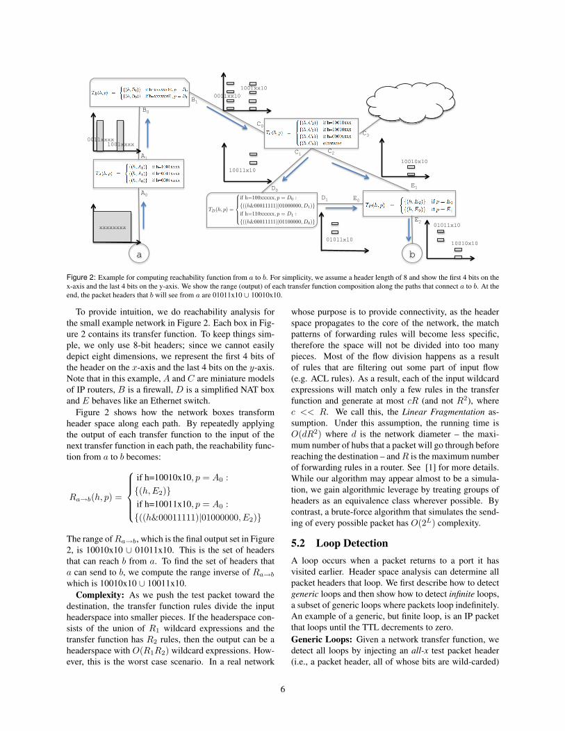
In our scenario, Alice – a networking researcher – in-vents a new loose source routing protocol, IP*. IP* al-lows a source to specify the sequence of middle boxesthat a packet must pass through. Alice’s protocol has theheader format shown in Figure 10.a. IP* works exactlylike normal IP, except that it updates the header at thefirst router where a packet enters the IP* network. Figure10.b shows an example of header update for a stack sizeof three. The header update operation sets the currentsource address to the “sender IP address” field, rewritesthe destination IP address to the address at the top of thestack, and rotates all the IP addresses in the stack. Afterprocessing, a destination middlebox swaps the destina-tion and source IP addresses and resends the packet to arouter. Alice designs IP* to allow tunneling across exist-ing IP networks.

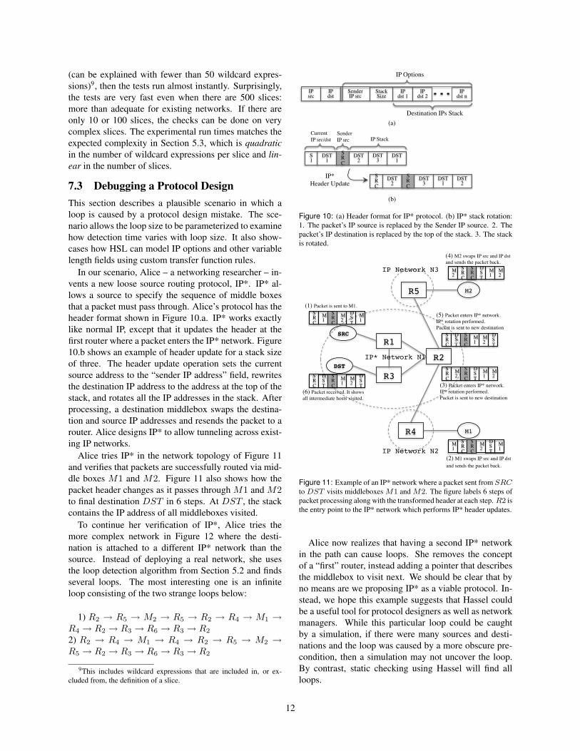
Alice tries IP* in the network topology of Figure 11and verifies that packets are successfully routed via mid-dle boxes M1 and M2. Figure 11 also shows how thepacket header changes as it passes through M1 and M2to final destination DST in 6 steps. At DST , the stackcontains the IP address of all middleboxes visited.

To continue her verification of IP*, Alice tries themore complex network in Figure 12 where the desti-nation is attached to a different IP* network than thesource. Instead of deploying a real network, she usesthe loop detection algorithm from Section 5.2 and findsseveral loops. The most interesting one is an infiniteloop consisting of the two strange loops below:

1) R2 → R5 → M2 → R5 → R2 → R4 → M1 →R4 → R2 → R3 → R6 → R3 → R2

2) R2 → R4 → M1 → R4 → R2 → R5 → M2 →R5 → R2 → R3 → R6 → R3 → R2

9This includes wildcard expressions that are included in, or ex-cluded from, the definition of a slice.

IP src

IP dst

Sender IP src

Stack Size

IP dst 1

IP dst 2

IP dst n

IP Options

Destination IPs Stack

S1

SRC

DST 1

DST 2

DST 3

DST 1

SRC

SRC

DST 2

DST 3

DST 1

DST 2

IP* Header Update

IP Stack Sender IP src

Current IP src/dst

(a)

(b)

Figure 10: (a) Header format for IP* protocol. (b) IP* stack rotation:1. The packet’s IP source is replaced by the Sender IP source. 2. Thepacket’s IP destination is replaced by the top of the stack. 3. The stackis rotated.

R1!

R2!

R3!

SRC!

DST!

R5!

R4!

M2!

IP Network N3!

IP Network N2!

M1!

SRC

M1

M2

SRC

DST

M1

M1

SRC

M2

SRC

DST

M1

SRC

M2

DST

SRC

M1

M2

M2

SRC

DST

SRC

M1

M2

SRC

DST

M1

SRC

M2

DST

SRC

DST

M1

SRC

M2

DST

(1) Packet is sent to M1.

(2) M1 swaps IP src and IP dst and sends the packet back.

(3) Packet enters IP* network. IP* rotation performed. Packet is sent to new destination

(4) M2 swaps IP src and IP dst and sends the packet back.

(6) Packet received. It shows all intermediate hosts visited.

(5) Packet enters IP* network. IP* rotation performed. Packet is sent to new destination

IP* Network N1!

Figure 11: Example of an IP* network where a packet sent from SRCto DST visits middleboxes M1 and M2. The figure labels 6 steps ofpacket processing along with the transformed header at each step. R2 isthe entry point to the IP* network which performs IP* header updates.

Alice now realizes that having a second IP* networkin the path can cause loops. She removes the conceptof a “first” router, instead adding a pointer that describesthe middlebox to visit next. We should be clear that byno means are we proposing IP* as a viable protocol. In-stead, we hope this example suggests that Hassel couldbe a useful tool for protocol designers as well as networkmanagers. While this particular loop could be caughtby a simulation, if there were many sources and desti-nations and the loop was caused by a more obscure pre-condition, then a simulation may not uncover the loop.By contrast, static checking using Hassel will find allloops.

12

R6!

IP Network N4!

R7!

IP* Network N5!

R1!

R2!

R3!

SRC!

DST!

R5!

R4!

M2!

IP Network N3!

IP Network N2!IP* Network N1!

M1!

Figure 12: Alice’s second network topology can cause infinite loops.

0.01

0.1

1

10

100

1000

0 20000 40000 60000 80000 100000 120000 140000

Run

Tim

e (S

econ

d)

Number of Transfer Function Rules

2 Middleboxes 3 Middleboxes 4 Middleboxes Stanford Backbone

Figure 13: Running time of loop detection algorithm on Ip* network

Figure 13 shows the per-port performance of our in-finite loop detection algorithm for the ports participat-ing in the loops. We varied the number of middle boxesconnected to R2 (e.g., M1 and M2) and the number ofrouter forwarding entries. For four middle boxes, theloop has a length of 72 nodes! Finding a large and com-plex loop in less than four minutes — for a network with100,000 forwarding rules and custom actions — usingless than 50 lines10 of python code (figure 14) demon-strates the power of the Header Space framework.

8 LimitationsHeader space analysis is designed for static analysis,to detect forwarding and configuration errors. It is nopanacea, serving as one tool among many needed by pro-tocol designers, software developers, and network oper-ators. For example, while header space analysis mighttell us that a routing algorithm is broken because rout-ing tables are inconsistent, it does not tell us why. Evenif the routing tables are consistent, header space analy-sis offers no clues as to whether routing is efficient ormeets the objectives of the designer. Despite this, headerspace analysis could play a similar role in networks aspost-layout verification tools do in chip design, or staticanalysis checkers do in compilation. It checks the lowlevel output against a set of universal invariants, with-out understanding the intent or aspirations of the proto-col designer. To analyze protocol correctness, other ap-

10Not counting the underlying Hassel implementation

def detect_loop(NTF, TTF, ports, test_packet): loops = [] for port in ports: propagation = [] p_node = {} p_node["hdr"] = test_packet p_node["port"] = port p_node["visits"] = [] p_node["hs_history"] = [] propagation.append(p_node) while len(propagation)>0: tmp_propag = [] for p_node in propagation: next_hp = NTF.T(p_node["hdr"],p_node["port"]) for (next_h,next_ps) in next_hp: for next_p in next_ps: linked = TTF.T(next_h,next_p) for (linked_h,linked_ports) in linked: for linked_p in linked_ports: new_p_node = {} new_p_node["hdr"] = linked_h new_p_node["port"] = linked_p new_p_node["visits"] = list(p_node["visits"]) new_p_node["visits"].append(p_node["port"]) new_p_node["hs_history"] = list(p_node["hs_history"]) new_p_node["hs_history"].append(p_node["hdr"]) if len(new_p_node["visits"]) > 0 \ and new_p_node["visits"][0] == linked_p: loops.append(new_p_node) print "loop detected" elif linked_p not in new_p_node["visits"]: tmp_propag.append(new_p_node) propagation = tmp_propag return loops

Figure 14: Loop Detection Code

proaches, such as [14] should be used.Similarly, while our approach can pinpoint the specific

entry in the forwarding table or line in the configurationfile that causes a problem, it does not tell us how or whythose entries were inserted or how they will be evolved asthe box receives future messages. Finally, like all staticcheckers, our formalism and tools cannot deal well withchurn in the network, except to periodically run it basedon snapshots: thus it can only detect problems that persistlonger than the sampling period.

9 Related WorkThe notion of a transfer function in our work is similar toASE mapping defined in axiomatic routing [14], wherethe authors develop tools to analyze a variety of proto-cols. Header space analysis makes no attempt to ana-lyze protocols; instead, it tackles the problem of indepen-dently checking if their output creates conflicts. Roscoe’spredicate routing [8] introduces the notion of pushing atest packet (as used in our reachability and loop detectionalgorithms) when designing routing mechanisms, ratherthan for static checking as we do. Xie’s reachability anal-ysis [4] uses test packets to determine reachability (notloop detection) for the special case of TCP/IP networks.The static analysis tools described in [9, 10, 11] are de-signed specifically for TCP/IP firewalls, and Feamster’swork in [15] finds reachability failures in BGP routers.

Header space analysis is broader in two ways. First, itis a framework that can identify a range of network con-figuration problems. Second, the algorithms developedin this framework are independent of protocols. Finally,note that model checking, SAT solvers, and TheoremProvers are other commonly used frameworks for veri-fication [16]. However, when these frameworks detecta violation of a specification (e.g., reachability) they arelimited to providing a single counterexample and not the

13

full set of failed packet headers that header space analysisprovides.

10 ConclusionsOur paper introduces Header Space Analysis: a generalframework for reasoning about arbitrary protocols, andfor finding common failures, or accidents. By parsingrouting and configuration tables automatically, we showthat header space analysis can be used in existing net-works where protocol interactions are increasingly com-plex. As we saw in the Stanford backbone and noted by[12], while individual protocols use automated mecha-nisms to prevent internal problems, managing many pro-tocols simultaneously is a manual and error-prone busi-ness. Header Space Analysis can also be used in emerg-ing networks, where new protocols can be added dynam-ically. It can give network operators the confidence toadopt new protocols, or new slicing mechanisms — theframework can be used to create comprehensive check-ers that can be used by network operators to pro-activelyavoid (or retroactively investigate) accidents.

Our personal story is that we set out to create a ge-ometric model to better understand slicing. Along theway, we discovered how simple it is to analyze net-works using Network Transfer Functions (Ψ). We foundthat checking for a given violation was surprisingly easywhen expressed using this high level abstraction, allow-ing elegant expression and simple implementation as ourcode snippets (see Figure 14) suggest.

We have work to do to improve the performance ofour prototype Hassel implementation. A first round ofoptimization reduced running time by five orders of mag-nitude, making Hassel perform well for production net-works with a few dozen routers, adequate for most en-terprises and campuses. With simple fixes (e.g. exploit-ing 64-bit arithmetic, using compiled languages ratherthan Python, and harnessing the parallelism of multicorechips) we expect another 2-3 orders of magnitude perfor-mance gain. We expect running time of a complete looptest for a campus backbone to be reduced from about1,000 seconds to less than 10 seconds. Even more op-timizations are apparent, such as using a Karnaugh-Mapto reduce the size of header space after each transforma-tion. There is also scope for checking updates incremen-tally, by analyzing loops and reachability once, and thenseeing how a new rule (or slice) changes the result.

We have other work ahead of us: we would like to cre-ate tools that create test packets to dynamically sampleheader space to detect faults in an operational network.We also hope to explore the notion of how secure, orhow fault-tolerant, a network is by finding the “distance”between the current status of the network, and differentfailure conditions — analogous to Hamming distance.

Accidents will happen in the best regulated of net-works; but the judicious use of checkers such as ours canreduce their probability.

11 AcknowledgementWe would like to thank our shepherd, Ranveer Chandraand the anonymous reviewers for their valuable com-ments. We also thank our network admin, Johan vanReijendam, for collecting network data for us. The firstauthor was supported by a Stanford Graduate Fellowship(SGF) while doing this research.

References[1] P. Kazemian, G. Varghese, N. McKeown, Header Space Analysis, Technical

Report, http://stanford.edu/˜kazemian/hsa.pdf

[2] Header Space Library (Hassel) http:/stanford.edu/˜kazemian/hassel.tar.gz

[3] T. V. Lakshman and D. Stiliadis, High-Speed Policy-based Packet Forward-ing Using Efficient Multi-dimensional Range Matching, Proc. ACM SIG-COMM, pp. 191–202, 1998.

[4] G. Xie, J. Zhan, D. Maltz, H. Zhang, A. Greenberg, G. Hjalmtysson, and J.Rexford, On Static Reachability Analysis of IP Networks, Proc. IEEE INFO-COM Conference, 2005.

[5] N. McKeown, T. Anderson, H. Balakrishnan, G. Parulkar, L. Peterson, J.Rexford, S. Shenker, and J. Turner, OpenFlow: Enabling Innovation inCampus Networks, ACM SIGCOMM Computer Communication Review,Volume 38, Number 2, 2008.

[6] R. Sherwood, G. Gibb, K.K Yap, G. Appenzeller, M. Casado, N. McKe-own, G. Parulkar, Can the Production Network Be the Test-bed?, USENIXSymposium on Operating Systems Design & Implementation (OSDI) 2010.

[7] R. Draves, C. King, S. Venkatachary, B. Zill, Constructing optimal IP routingtables, 1999 Proc. IEEE INFOCOM, 1999.

[8] T. Roscoe, S. Hand, R. Isaacs, R. Mortier, P. Jardetzky Predicate Routing:Enabling Controlled Networking Proc. of 1st Workshop on Hot Topics inNetworks, 2002

[9] L. Yuan, J. Mai, Z. Su, H. Chen, C-N. Chuah, and P. Mohapatra, FIREMAN:A Toolkit for Firewall Modeling and Analysis, 2006 IEEE Symposium onSecurity and Privacy, pp. 213-228

[10] Y. Bartal, A. J. Mayer, K. Nissim, and A. Wool. Firmato:A novel firewallmanagement toolkit, Proc. 20th IEEE Symposium on Security and Privacy,1999.

[11] A. Mayer, A. Wool, and E. Ziskind, Fang: A firewall analysis engine, Proc.IEEE Symposium on Security and Privacy, 2000.

[12] F. Le, G. Xie, D. Pei, J. Wang, and H. Zhang, Shedding Light on the GlueLogic of the Internet Routing Architecture, Proc. ACM SIGCOMM Confer-ence, 2008.

[13] F. Le, G. Xie, and H. Zhang, Understanding Route Redistribution, Proc.IEEE ICNP 2007 Conference, Beijing, China, 2007.

[14] M. Karsten, S. Keshav , S. Prasad , M. Beg An Axiomatic Basis for Com-munication Proc. ACM SIGCOMM Conference, 2007.

[15] N. Feamster, H. Balakrishnan, Detecting BGP configuration faults withstatic analysis, Proc. of the 2nd conference on Symposium on NetworkedSystems Design & Implementation - Volume 2, NSDI’05,

[16] H. Mai, et. al., Debugging the data plane with anteater Proc. ACM SIG-COMM Conference, 2011.

[17] E. M. Clarke, O. Grumberg, D. A. Peled, Model Checking, MIT Press,1999.

[18] S. Brown, Z. Vranesic, Fundamentals of Digital Logic with Verilog Design,McGraw-Hill, 2003.

[19] Global Environment for Network Innovations (GENI),http://www.geni.org

[20] The Health Insurance Portability and Accountability Act (HIPAA),http://www.hhs.gov/ocr/privacy/

14