Hazardous waste sites and housing appreciation rates

Journal of Environmental Economics and Management 45 (2003) 166–176

Hazardous waste sites and housing appreciation rates

Jill J. McCluskeya,* and Gordon C. Rausserb,1

aDepartment of Agricultural Economics, Washington State University, PO Box 646210, Pullman, WA 99164-6210, USAbDepartment of Agricultural and Resource Economics, University of California, Berkeley, CA 94720, USA

Received 7 February 2000; revised 9 July 2001

Abstract

Housing appreciation rates reflect the speed of the market’s adjustment to equilibrium. The dynamiceffect of a hazardous waste site is analyzed by investigating the causal relationship between housingappreciation rates and house location in relation to a hazardous waste site using resale data from individualsales transactions in Dallas County, Texas. The results indicate that residential property owners in closeproximity to the hazardous waste site experienced lower housing appreciation rates after the time periodwhen the US Environmental Protection Agency identified the site. The adjustment to equilibrium, asreflected in differential housing appreciation rates, can be quite lengthy in response to the identification andcleanup process for a hazardous waste site. The results suggest that cleanup actions are not as important asnew information that the area surrounding the site is a dangerous place.r 2003 Elsevier Science (USA). All rights reserved.

Keywords: Housing appreciation rates; Hazardous waste site

1. Introduction

The public’s increasing awareness of environmental risks is reflected in the negative impact ofenvironmental contamination on property values in the real estate market. Although the effects ofenvironmental contamination on property values have been studied, the current body of literatureon the effects of locally undesirable land uses does not address the adjustment of property valuesto the discovery and cleanup of environmental contamination. Kiel and McClain [10] come theclosest to analyzing this issue. They examined the effect of an incinerator siting on housingappreciation rates. However, their study was limited to siting and operation and did not consider

*Corresponding author.

E-mail address: [email protected] (J.J. McCluskey).1Member, Giannini Foundation of Agricultural Economics.

0095-0696/03/$ - see front matter r 2003 Elsevier Science (USA). All rights reserved.

doi:10.1016/S0095-0696(02)00048-7

any time period after the incinerator was shut down or removed. In contrast, this paperexamines the impact of environmental contamination and cleanup on residential propertyvalue appreciation rates by analyzing data from before identification of the hazardouswaste site and before, during, and after cleanup has been completed and a during a period ofnew concern. Consequently, it is possible to empirically investigate longer-run marketadjustments.

Stigma is a negative attribute of real estate acquired by the discovery of contamination andreflected in price Elliot-Jones [4]. Using a neighborhood turnover model with external economies,McCluskey and Rausser [15] show that both temporary stigma and permanent stigma are possibleequilibrium outcomes after discovery and cleanup of a hazardous waste site. If the priceadjustment after the cleanup of a hazardous waste site is gradual, as opposed to immediate andpermanent, then the cost to the residential property owner cannot be measured immediately aftercleanup.

The duration of stigma has significant legal ramifications. When the courts award stigmadamages based on unrealized losses in property values, they are implicitly assuming that stigmadamage is permanent and does not change over time. If stigma is temporary and compensation isawarded based on unrealized losses, then plaintiffs may receive a windfall. On the other hand, ifthe Courts consider the stigma to be temporary, then the property owner may receive nocompensation, even though he or she has experienced a real loss. The loss emerges from the factthat during the period of temporary stigma, the asset is less liquid. Illiquid assets, all other thingsequal, generally have higher returns to compensate investors for what is given up in terms ofliquidity. Consequently, determining the effect of environmental contamination and cleanup onhousing appreciation rates is necessary to accurately estimate the true cost of the contaminationto residential property owners.

In this paper, appreciation rates are calculated for houses in Dallas County, Texas, whichcontains the RSR hazardous waste site. The RSR lead smelter in West Dallas, which operatedfrom 1934 to 1984, caused soil contamination from air emissions and slag material. The slagmaterial was used as fill in yards and driveways in nearby residences. The data set used in ouranalysis covers the period 1979–95 and includes 31,974 repeat sale observations.

A repeat sales hybrid approach is advanced to examine the relationship between housingappreciation rates and the location of the house in relation to the hazardous waste site using datafrom individual sales transactions in Dallas County, Texas. The dynamic effects of the smelter arethen analyzed by estimating its effect on housing appreciation rates and testing whether the effectchanges over time.

2. Previous studies

Many authors have used property value data to value environmental attributes and, morespecifically, study the impact of hazardous waste sites. Studies have shown that negative attitudestoward facilities which pose nuisance, health or environmental risks are strong and geographicallyextensive [13]. Dale et al. [3], Ketkar [8], Kiel [9], Kohlhase [11], Michaels and Smith [18],Nelson et al. [19], Reichert et al. [21], Smith and Desvousgous [23], Smolen et al. [24], and

J.J. McCluskey, G.C. Rausser / Journal of Environmental Economics and Management 45 (2003) 166–176 167

Thayer et al. [25] have consistently found that proximity to hazardous waste sites and other locallyundesirable land uses (LULUs) has a negative impact on property values.2

Two previous studies have analyzed the direct effect of the RSR smelter on house prices. Daleet al. [3] analyzed the effect of the RSR smelter on price levels. They quantified the discontinuityof the distance price gradient surrounding the smelter by including dummy variables for twospecific neighborhoods. As a result, they concluded that there was no long-term stigma associatedwith the RSR smelter. In contrast, McCluskey and Rausser [15] specifically allowed for theinfluence of the smelter to diminish with distance. They found that houses within 1.2 miles of thesmelter experienced stigma. This analysis complements the previous analyses of the effect of RSRsmelter by considering the rate of price adjustment.

The repeat sale approach has been used extensively in real estate economics [20] and applied tomeasuring hazardous waste site damages [17]. Crone et al. [2] compared five methods ofestimating housing appreciation rates and found the repeat sales method to be the most accurate.

The appreciation rate of house prices can be used to calculate the user cost of owner-occupiedhousing. It is also used to compare the rate of return on investment in residential properties toother types of assets. Kiel and McClain [10] found that housing appreciation rates were affected asearly as construction began on a locally undesirable land use, and the adjustment continuedseveral years after the facility began operation. Greenberg et al. [6] and Greenberg et al. [7]analyzed the effect of hazardous waste sites on housing appreciation rates. However, these twostudies were based on aggregate and survey data rather than individual sales transactions.

3. Model of housing appreciation rates

The dynamic effects of the hazardous waste site can be examined by estimating its effect onhousing appreciation rates. The annual appreciation rate, r; is defined as

ð1þ rÞðt�tÞ ¼ Pt

Pt; ð1Þ

where t is the year of the first sale, and t is the year of the second sale. Solving for r; we obtain

r ¼ explnðPt=PtÞ

t � t

� �� 1: ð2Þ

The appreciation rate was calculated for each house in the resale data set. Following Kiel andMcClain [10], the annual appreciation rate for each house (multiplied by 100) is used as thedependent variable in regressions with variables that may affect the housing appreciation rates,including school district, a sale during the ‘‘boom’’ period (1979–85) or during the ‘‘bust’’ period(1987–92), changes in neighborhood demographics, the interest rate, and the distance to the RSRsite as the explanatory variables. Also following Kiel and McClain [10], we allow the effect ofdistance to the RSR site to vary over time by multiplying the distance variable by indicatorvariables for six event-driven time periods.

Previous studies, such as McClelland [14], have found that the impact of the waste site onproperty values dissipated rapidly with distance. Following Thayer et al. [25], we use a linear

2For additional cites, see [5], which provides a comprehensive survey of empirical results.

J.J. McCluskey, G.C. Rausser / Journal of Environmental Economics and Management 45 (2003) 166–176168

spline function to allow for discontinuities of the housing appreciation rate gradient. Formally, letr be the housing appreciation rate, let x1 be the distance to the site, let x2 be the distance at whichthe influence of the site diminishes, let g12g6 be the indicator variables for time periods 1–6, andlet x32xn be the other explanatory variables. The estimated model is then the following:

r ¼ b0 þX6

i¼1

bigix1 þX6

i¼1

b6þigid2ðx1 � x2Þ þXn

i¼3

b12þixi þ e; ð3Þ

where d2 ¼1 if x14x2

0 otherwise

�; and e is an error term. Eq. (3) was estimated with a linear spline

function with a discontinuity in the gradient at 1.2 miles from the RSR site.3

The focus of this paper is the adjustment to equilibrium of housing prices for properties in closeproximity to a hazardous waste site as new information emerges from the cleanup process.Consequently, the functional form of the distance variable must (1) be flexible and (2) allow foreffect of the hazardous waste site to dissipate rapidly with distance. A linear spline functionsatisfies both of these requirements. First, the spline function is more flexible than imposingcertain specific functional forms that do not apply to all time periods. If different functional formswere used for different time periods, then the results would not be comparable across periods.Second, linear spline functions allow for there to be one rate for distance up to a critical point andthen an adjustment to the rate after that point. Relevant to the second point, the public often hasa perception of where the threshold is for the sphere of influence of the hazardous waste site is. Alinear spline function is well suited to deal with abrupt changes in perceptions of location, since itallows for discontinuities in the gradient with respect to distance. For example, the spline functionperforms better than a quadratic in distance based on minimizing the sum of squared errors.

4. Background and data

The RSR lead smelter is located in the central portion of Dallas County, approximately 6 mileswest of downtown Dallas. The smelter operated from 1934 to 1984 and was purchased in 1971 bythe RSR Corporation. The smelter emitted airborne lead, which contaminated the soil in thesurrounding areas. Lead debris created by the smelter was used in the yards and driveways ofsome West Dallas residences. In 1981, the EPA found health risks, and RSR agreed to remove anycontaminated soil in the neighborhoods surrounding the RSR site using standards that wereconsidered protective of human health at the time. In 1983 and 1984, additional controls wereimposed by the City of Dallas and the State of Texas. In 1984, the smelter was sold to the MurmurCorporation who shut the smelter down permanently. In 1986, a court ruled that the cleanup wascomplete.

In 1991, the Center for Disease Control (CDC) lowered the blood level of concern for childrenfrom 30 to 10 mg of lead per deciliter of blood. Low-level lead exposure in childhood may cause

3The closest estimable critical point is 1.2 miles. Using a grid search approach with the objective of minimizing the

sum of squared errors, McCluskey and Rausser [15] found that 1.2 miles was the point where the influence of the RSR

smelter diminished in terms of its effect on price level. The logic of using the closest estimable critical point is that the

affected area is very limited.


reductions in intellectual capacity and attention span, reading and learning disabilities,hyperactivity, impaired growth, or hearing loss [12]. Also in 1991, the State of Texas foundhazardous waste violations at the smelter. In 1993, the RSR smelter was placed on the SuperfundNational Priorities List (NPL).

The analysis covers the impact of the smelter on property values over six event-driven timeperiods: (1) pre-1981, when the smelter operated but health risks were not officially identified norpublicized; (2) 1981–83, when health risks from soil contamination were officially identified; (3)1984–1986, when cleanup was initiated and a Court ruled it was completed; (4) 1987–90, initialperiod after cleanup was ruled completed; (5) 1991–93, when new concerns arose and additionalcleanup occurred; and (6) 1994–95, after the RSR was placed on the National Priorities List as aSuperfund Site. Slovic et al. [22] provides support for the use of event-driven time periods. Inparticular, they argue that social amplification of risk is triggered by the occurrence of an adverseevent.4

The repeat sales data set includes variables describing price5 and attributes of single-family,detached homes sold over the period 1977–95 in Dallas County, Texas (Dallas County AppraisalDistrict). Summary statistics of the variables used in the analysis are presented in Table 1. The

Table 1

Resale data: summary statistics

Variable Mean Std dev. Minimum Maximum

Housing appreciation rate �2.9839 15.3173 �90.1295 882.2275

2nd sale during boom period 0.1001 0.3001 0 1

2nd sale during bust period 0.4785 0.4995 0 1

Change in % African Amer. 2.9690 4.7854 �39.2848 56.5849

Change in % Hispanic 2.6957 4.7755 �58.7005 58.4056

Change in % poverty 1.3650 2.7902 �15.7069 38.6845

Interest rate 11.3065 2.9612 6 18.8700

Log of years between sales 1.5351 0.7044 0 2.7726

Carrollton/Farmers Branch 0.080597 0.272219 0 1

Cedar Hill 0.014387 0.119081 0 1

Garland 0.136893 0.343739 0 1

Highland Park 0.02746 0.163422 0 1

Irving 0.054544 0.227092 0 1

Lancaster/Wilmer Hutchins 0.009351 0.096251 0 1

Mesquite/Sunnyvale 0.065272 0.247009 0 1

No district 0.045912 0.209298 0 1

Coppell 0.026647 0.161051 0 1

Grand Prairie 0.034528 0.182584 0 1

Richardson 0.150278 0.35735 0 1

Desoto 0.022143 0.147151 0 1

Duncanville 0.033402 0.179687 0 1

Distance to RSR 11.8718 4.1417 1.0409 23.0215

N=31,974

4Slovic et al. [22, p. 685.]5Prices are deflated using the shelter housing price index (1982–84=100) from the Economic Report of the President.


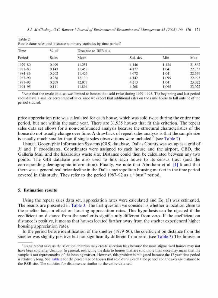
price appreciation rate was calculated for each house, which was sold twice during the entire timeperiod, but not within the same year. There are 31,935 houses that fit this criterion. The repeatsales data set allows for a non-confounded analysis because the structural characteristics of thehouse do not usually change over time. A drawback of repeat sales analysis is that the sample sizeis usually much smaller than if single sales observations were included.6 (see Table 2)

Using a Geographic Information Systems (GIS) database, Dallas County was set up as a grid ofX and Y coordinates. Coordinates were assigned to each house and the airport, CBD, theGalleria Mall and the hazardous waste site. Distance could then be calculated between any twopoints. The GIS database was also used to link each house to its census tract (and thecorresponding demographic information). Finally, we note that Abraham et al. [1] found thatthere was a general real price decline in the Dallas metropolitan housing market in the time periodcovered in this study. They refer to the period 1987–92 as a ‘‘bust’’ period.

5. Estimation results

Using the repeat sales data set, appreciation rates were calculated and Eq. (3) was estimated.The results are presented in Table 3. The first question we consider is whether a location close tothe smelter had an effect on housing appreciation rates. This hypothesis can be rejected if thecoefficient on distance from the smelter is significantly different from zero. If the coefficient ondistance is positive, it means that houses located farther away from the smelter experienced higherhousing appreciation rates.

In the period before identification of the smelter (1979–80), the coefficient on distance from thesmelter was slightly positive but not significantly different from zero. (see Table 3) The houses in

Table 2

Resale data: sales and distance summary statistics by time perioda

Time % of Distance to RSR site

Period Sales Mean Std. dev. Min Max

1979–80 0.099 11.251 4.146 1.124 21.862

1981–83 0.143 11.452 4.177 1.041 22.353

1984–86 0.202 11.426 4.072 1.041 22.679

1987–90 0.238 12.130 4.142 1.095 22.923

1991–93 0.208 12.077 4.213 1.041 23.022

1994–95 0.111 11.894 4.268 1.095 23.022

aNote that the resale data set was limited to houses that sold twice during 1979–1995. The beginning and last period

should have a smaller percentage of sales since we expect that additional sales on the same house to fall outside of the

period studied.

6Using repeat sales as the selection criterion may create selection bias because the most stigmatized houses may not

have been sold after cleanup. In general, restricting the data to houses that are sold more than once may mean that the

sample is not representative of the housing market. However, this problem is mitigated because the 17 year time period

is relatively long. See Table 2 for the percentage of houses that sold during each time period and the average distance to

the RSR site. The statistics for distance are similar to the entire data set.


close proximity to the smelter sold at lower price levels before identification, suggesting that themarket already had already taken account of the smelter as a disamenity [3,15], but the rate ofappreciation was not significantly different from the rest of the market. Since distance did notaffect appreciation rates during this opening period, we consider this as the opening equilibriumbefore any new information or publicity. Although the magnitudes vary in reaction toinformation, media coverage, and events that occurred over time, the coefficients on distanceare positive and significant for all of the subsequent time periods. The distance coefficient became

Table 3

Estimation results, dependant variable: appreciation rate

Parameter T for H0:

Variable estimate parameter=0 Prob.4|T|

Intercept 0.0164 0.031 0.9756

2nd sale during boom period 2.2680 4.359 0.0001

2nd sale during bust period �1.5809 �5.678 0.0001

Change in % African Amer. 0.0382 1.733 0.0832

Change in % Hispanic �0.0715 �3.160 0.0016

Change in % poverty �0.1037 �2.649 0.0081

Interest rate at 2nd sale 0.6583 16.735 0.0001

Log of years between sales �6.3959 �35.895 0.0001

Carrollton/Farmers Branch �0.7474 �2.013 0.0441

Cedar Hill �2.7302 �3.789 0.0002

Garland 0.1120 0.294 0.7687

Highland Park 1.4744 2.780 0.0054

Irving �1.7089 �4.469 0.0001

Lancaster/Wilmer Hutchins �1.1969 �1.342 0.1795

Mesquite/Sunnyvale �0.5664 �1.381 0.1672

No district �1.2728 �2.656 0.0079

Coppell �0.5487 �0.981 0.3264

Grand Prairie �1.7858 �3.805 0.0001

Richardson 0.2966 0.959 0.3374

Desoto �2.5393 �4.157 0.0001

Duncanville �2.9331 �5.992 0.0001

Distance to RSR (079–080)a, b1 0.1926 0.062 0.9509






Adjustment (079–080)a, b7 0.0755 0.022 0.9824

Adjustment (081–083)a, b8 �3.1203 �2.603 0.0093

Adjustment (084–086)a, b9 �6.9255 �8.487 0.0001

Adjustment (087–090)a, b10 �2.0554 �3.839 0.0001

Adjustment (091–093)a, b11 �2.5843 �5.226 0.0001

Adjustment (094–095)a, b12

�6.1059 �10.332 0.0001

F statistic =105.56aDates indicate that the second sale of the home occurred during the specified period.


positive and significant during the identification period (1981–83) and increased in magnitudeduring the cleanup period (1984–86). In the first period after cleanup (1987–90), the distancecoefficient was much smaller in magnitude but still highly significant. In the subsequent periodafter cleanup (1991–93), the distance coefficient increased in magnitude and became moresignificant. This period coincides with additional concern and media coverage and the CDCannouncement about the dangers of lower-level lead poisoning. The distance coefficient actuallyincreased in magnitude during the last period of the study (1994–95), most likely in response tobeing placed on the National Priorities List as a Superfund site. This suggests that the housingmarket in Dallas had still not settled into a new equilibrium in 1995.

The adjustment coefficients in Table 3 are the estimated values for b7 through b12 in [3]. Beyondthe critical point of 1.2 miles, the appreciation rate gradient is equal to the sum of the relevantadjustment coefficient and the distance coefficient. The hypothesis that the effect of the smelter isconstant with distance can be rejected if the coefficients for the adjustment variables are differentfrom zero. The coefficients on the adjustment variables are significantly different from zero for allbut the first period. As expected, in all but the first period, the coefficient for the adjustment at 1.2miles is negative. The interpretation is that the adjustment coefficient is negative because theinfluence of the smelter diminishes with distance.

As the following examples show, the predicted effects of distance from the smelter onhousing appreciation rates are reasonable. If a house sold for the second time in 1985 and islocated four miles from the smelter, we obtain an effect on appreciation rate from distance of5.26%.7 If the same house were located ten miles away from the smelter, we obtain a 0.62%positive effect on the appreciation rate. For properties further out, the effect on the appreciationrate from becomes negative. If a house sold for the second time in 1987 and is located four milesfrom the smelter, we obtain a 1.13% positive effect the appreciation rate. Finally, if a house soldfor the second time in 1983 and is located four miles from the smelter, we obtain a 0.75% positiveeffect.

Although the focus of this paper is on the effect of a hazardous waste site on housingappreciation rates, there are some additional observations that can be made based on theestimation results before we consider the hypothesis tests for changes in the distance coefficient.Higher interest rates resulted in significantly higher rates of appreciation. A longer time betweenfirst and second sales of the house is associated with a significantly lower rate of appreciation.Certain school districts had significantly positive or negative effects on appreciation rates. Asecond sale during the ‘‘boom’’ period (1979–85) positively and significantly affected appreciationrates, while a second sale during the ‘‘bust’’ period (1987–92) negatively and significantly affectedappreciation rates. Finally, increases in the percentage of poverty and the percentage of Hispanicresidents in the census tract in which the house is located negatively influenced appreciation rates,while increases in the percentage of African American residents increased appreciation rates.From this, one could conclude that certain African American neighborhoods are becoming moredesirable locations, as reflected in the real estate market.

We tested a series of hypotheses regarding the effect of events/information/time on howproximity to the smelter affects housing appreciation rates over time. In each hypothesis test, wetested whether the coefficient for distance from smelter for a particular time period is equal to the

74 miles� 6.1651+(4 miles–1.2 miles)� (�6.9255)=5.26.


coefficient on distance in an adjacent time period.8 The results of the tests are presented in Table4. We found that the coefficient for distance for the identification period (1981–83) was greaterthan but not significantly different from coefficient for distance for the period before identification(1979–80). However, the coefficient for distance for the identification period (1981–83) wassignificantly less than the coefficient for distance for the cleanup period (1984–86), which was aperiod of intense media coverage [16]. Further, the coefficient for distance for the cleanup period(1984–86) was significantly greater than the first post-cleanup period (1987–90), which could beinterpreted to mean that the effect of the smelter was diminishing. However, this trend did notcontinue. The distance coefficient increased but not significantly from the first post-remediationperiod (1987–90) to the second post cleanup period, a period of new concern (1991–93). Finally, inthe subsequent period after being named to the National Priorities List (NPL), the coefficient ondistance significantly increased.

The findings of how appreciation rates changed during the identification, remediation, post-remediation, and Superfund nomination periods go against standard economic thinking thatremediation should increase the property values of the properties in close proximity to thehazardous waste site rather than hurt them. The results suggest that actions are not as importantas new information that the area surrounding the site is a dangerous place. It may be the case thatplacement on the NPL is a large signal to individuals that the site is contaminated and does notprovide assurance that the site will be cleaned in the near future.

Table 4

Hypotheses testing results (for distance coefficients

Hypothesis F statistic P-value Reject at a ¼ 0:05?

Before identification (1979–80) vs. 0.465 0.4955 No

identification/before cleanup (1981–83)

bdistance;79�80 � bdistance;81�83 ¼ 0a

Identification/before cleanup (1981–83) vs. 12.196 0.0005 Yes

cleanup (1984–86)

bdistance;81�83 � bdistance;84�86 ¼ 0

cleanup (1984–86) vs. 1st post cleanup 31.283 0.0001 Yes

(1987–90)


1st post cleanup (1987–90) vs. period of 1.454 0.2279 No

new concerns (1991–1993)


New concerns (1991–1993) vs. NPL listing

(1994–95) bdistance;91�93 � bdistance;94�95 ¼ 0

43.2405 0.0001 Yes

aUsing the notation from [3], this hypothesis is H0 : b1 � b2 ¼ 0: The other hypotheses can be similarly restated in the

notation from [3].

8Since the results confirm that the influence of the hazardous waste site on housing appreciation rates diminished

rapidly with distance, the hypotheses that housing appreciation rate gradients near the hazardous waste site are equal

across time are the ones that are of greatest interest for this study. Therefore, hypothesis tests for gradients beyond the

critical point of 1.2 miles are not reported.


6. Conclusions

Our results suggest that after new information, events, and publicity over time impacted theequilibrium of the housing market around a hazardous waste site. The appreciation rates forhouses located in close proximity to the RSR site were not significantly different from thoselocated farther away before the EPA identified the RSR site. After the new information andpublicity that were associated with the process of identification of the hazardous waste site,cleanup, additional concern and Superfund identification was revealed, individual housingappreciation rates were affected by proximity to the RSR hazardous waste site. The magnitude ofthe effect varied in reaction to the specific information, media coverage, and events. The value ofthe distance coefficient actually increased in magnitude during the last period of the study (1994–95), most likely in response to being placed on the National Priorities List as a Superfund site.From this analysis, we conclude that a long-run equilibrium was not yet reached sinceappreciation rates were significantly different across the Dallas housing market in 1994–95.

Our findings support Kiel and McClain’s [10] findings that the adjustment period to a newequilibrium can be quite long. The uncertainty that is associated with this adjustment toequilibrium is an additional consideration that buyers and sellers of homes near contaminatedsites and their lenders must take into account.

The Dallas housing market’s response to the publicity surrounding the RSR cleanup processand Superfund nomination was negative because cleanup signaled that the location wasdangerous to human health. This finding calls into question the validity of the standard riskassessment models in which it is the actual danger that matters rather than publicity. Given thelong record of risk assessment failing to convince the public, researchers and practitioners shouldbe aware of the entire impact that hazardous waste cleanup can have on surrounding propertyvalues.

Acknowledgments

The authors thank Zhihua Shen for computer programming assistance. This paper has alsobenefited from discussions with Ken Rosen, Robert Edelstein, and participants at the Real EstateSeminar at the Haas School of Business, U.C. Berkeley and comments from anonymousreviewers. All remaining errors are the responsibility of the authors. This work was supported byan EPA-NSF Grant. Jill McCluskey gratefully acknowledges financial support she received fromthe Fisher Center for Real Estate and Urban Economics at the Haas School of Business.

References

[1] J.M. Abraham, P.H. Hendershott, Bubbles in metropolitan housing markets, J. Housing Res. 7 (1996) 191–207.

[2] T.M. Crone, R.P. Voith, Estimating house price appreciation: a comparison of methods, J. Housing Econom. 2

(1992) 324–338.

[3] L. Dale, J.C. Murdoch, M.A. Thayer, Do property values rebound from environmental stigmas? Evidence from

Dallas County, Texas, Land Econom. 75 (1999) 311–326.

[4] M. Elliot-Jones, Stigma in light of recent cases, Nat. Res. Enviro. 56–59 (Spring 1996).


[5] S. Farber, Undesirable facilities and property values: a summary of empirical studies, Ecol. Econom. 24 (1998)

1–14.

[6] M.R. Greenberg, R.F. Anderson, Hazardous waste sites: the credibility gap, The Center for Urban Policy

Research, Rutgers, The State University of New Jersey 1984.

[7] M.R. Greenberg, J. Hughes, Impact of hazardous waste sites on property value and land use: tax assessors’

appraisal, Appraisal J. 61 (1993) 42–51.

[8] K. Ketkar, Hazardous waste sites and property values in the state of New Jersey, App. Econom. 24 (1992)

647–659.

[9] K.A. Kiel, Measuring the impact of the discovery and cleaning of identified hazardous waste sites on house values,

Land Econom. 71 (1995) 428–435.

[10] K.A. Kiel, K.T. McClain, The effect of an incinerator siting on housing appreciation rates, J. Urban Econom. 37

(1995) 311–323.

[11] J.E. Kohlhase, The impact of hazardous waste sites on housing values, J. Urban Econom. 30 (1991) 1–26.

[12] M.E. Kraft, D. Scheberle, Environmental justice and the allocation of risk: the case of lead and public health,

Policy Stud. J. 23 (1995) 113–123.

[13] M. Lindell, T.C. Earle, How close is close enough: public perceptions and the risks of industrial facilities, Risk

Anal. 3 (1983) 245–253.

[14] G.H. McClelland, W.D. Schulze, B. Hurd, The effects of risk beliefs on property values: a case study of a

hazardous waste site, Risk Anal. 10 (1983) 485–497.

[15] J.J. McCluskey, G.C. Rausser, Stigmatized asset value: is it temporary or long-term? Rev. Econom. Statist.,

forthcoming.

[16] J.J. McCluskey, G.C. Rausser, Estimation of perceived risk and its effect on property values, Land Econom. 77

(2001) 42–55.

[17] R. Mendelsohn, D. Hellerstein, M. Huguenin, R. Unsworth, R. Brazee, Measuring hazardous waste damages with

panel models, J. Environ. Econom. Management 22 (1992) 259–271.

[18] R.G. Michaels, V.K. Smith, Market segmentation and valuing amenities with hedonic models: the case of

hazardous waste sites, J. Urban Econom. 28 (1990) 223–242.

[19] A.C. Nelson, J. Genereux, M. Genereux, Price effects of landfills on house values, Land Econom. 68 (1992)

359–365.

[20] R.B. Palmquist, Measuring environmental effects on property values without hedonic regressions, J. Urban

Econom. 11 (1982) 333–347.

[21] A.K. Reichert, M. Small, S. Mohanty, The impact of landfills on residential property values, J. Real Estate Res. 7

(1992) 297–314.

[22] P. Slovic, et al., Perceived risk stigma and potential economic impacts of a high-level nuclear waste repository in

Nevada, Risk Anal. 11 (1991) 683–696.

[23] V.K. Smith, W.H. Desvousgous, The value of avoiding a LULU: hazardous waste disposal sites, Rev. Econom.

Statist. 68 (1986) 293–299.

[24] G.E. Smolen, G. Moore, L.V. Conway, The economic effects of hazardous chemical and proposed radioactive

waste landfills on surrounding real estate values, J. Real Estate Res. 7 (1992) 283–295.

[25] M. Thayer, H. Albers, M. Rahmatian, The benefits of reducing exposure to waste disposal sites: a hedonic housing

value approach, J. Real Estate Res. 7 (1992) 265–282.


Hazardous waste sites and housing appreciation rates

Documents

Transcript of Hazardous waste sites and housing appreciation rates