Hauth 2011 Cycloid

8/15/2019 Hauth 2011 Cycloid

http://slidepdf.com/reader/full/hauth-2011-cycloid 1/14

Int J Adv Manuf TechnolDOI 10.1007/s00170-011-3608-8

ORIGINAL ARTICLE

Cycloids for polishing along double-spiraltoolpaths in configuration space

Steffen Hauth · Lars Linsen

Received: 1 March 2011 / Accepted: 22 August 2011© Springer-Verlag London Limited 2011

Abstract An automated polishing process of free-formsurfaces requires a tool path that covers the entire sur-face equally and forms an overlapping pattern withoutvisible artifacts. The recently presented double-spiraltool paths assure a coverage of the entire surface witha continuous, non-overlapping path and low variationin distance between adjacent traces of the path. Webuild upon this approach by constructing cycloids of flexible radii that fill the space between adjacent traces.The use of cycloids mimics the cyclic movement whenpolishing by hand. The approach operates in a precom-puted configuration space (c-space) given in form of an adaptive quadrilateral heightfield mesh. Operatingin c-space avoids having to deal with the issues of patch-boundary oscillations or long, stretched trianglesin non-uniform rational b-spline surface or triangu-lar mesh representations, respectively. Our algorithmcomputes appropriate spheroids that are intersectedwith the c-space to compute the cycloids. We derive asmooth representation of the cycloids using arcs in arational Bézier formulation. We apply our approach toreal-world examples to demonstrate its effectiveness incovering the entire surface with the desired polishingmovements.

Keywords Tool path · Cycloid · Polishing ·

Free form surface · Configuration space

S. Hauth (B ) · L. LinsenSchool of Engineering and Science,Jacobs University Bremen gGmbH,Bremen, Germanye-mail: [email protected]

1 Introduction

In modern manufacturing practice, CNC machines arecommonly used to produce a variety family of function-ing surfaces andmolds. For this purpose, CAx-Softwareis essential when generating free form surfaces and toolpaths for the desired application, like milling, roughing,finishing, etc. Several strategies for the respective appli-cation have been developed and have been discussed inliterature widely (see [4, 7, 13, 14, 21]). The develop-ment of new machining types and techniques, like highspeed machining, has made it possible to reduce moldmanufacturing time. In spite of all the improvements,commonly the polishing processing for high-quality sur-faces is still manual labor. High-quality surfaces are, forexample, required for plastic injection molds. The needfor manual labor is based on the complexity of the pol-ishing process. To our knowledge, no properly workingalgorithm or strategy exists which enables polishing of arbitrary complex freeform surfaces.

A tool path for polishing applications has to fulfillseveral constraints: First, the tool path has to cover thewhole surface. Second, starting and stop movementsof the tool are hard to control, which likely causesartifacts on the surface. Although this is well-known, itis poorly documented in literature. Thus, the tool pathshall have only one starting and one stop movement.Third, patterns in the tool path are recognizable onthe surface, which reduces the quality of the result.Thus, polishing parts should be multidirectional ratherthan monotonic, in order to produce fewer undulationerrors (see [28]). Moreover, the multidirectional pol-ishing path is close to what is done by manual labor.Observing manual polishers, one can notice that theygo back on surface areas according to various patterns



Int J Adv Manuf Technol

such as cycloid polishing paths. A cycloid-shaped toolpath is known to produce good results (see [17, 18])and, hence, is considered as best practice for polishing.To our knowledge, no strategy exists, which fulfills allconstraints.

In this paper, we present a novel polishing strategy,which fulfills all mentioned constraints. In a first step,we cover the arbitrary free form surface with a doublespiral, where the starting and endpoint lie on the out-side of the spiral. This part of the algorithm is describedin detail in a previous publication [12]. The basic ideabehind the spiral is to start from offset curves andconnect them to two separate spirals. In their center,the two separate spirals are connected with a b-splinecurve to form the double spiral. The b-spline curve inthe center assures a bounded curvature in contrast tothe Archimedean spiral (see [11]). As a single doublespiral does not suffice to create a tool path on anysurface, we create multiple double spirals wheneverthe offset curves split into multiple components. Thesemultiple double spirals are connected appropriately toform one tool path that fulfills the requirements forhigh-quality finishing applications. In the second step,we overlay the double spiral with a flexible cycloidcurve. For creating the arcs of the cycloid curve, weintersect the surface with spheroids. Connecting thesearcs forms the cycloid curve. The ability to manipulatethe intersecting spheroids makes the cycloids flexiblein their radii in contrast to its standard counterparts.From now on, we refer to the two kinds of cycloidsas flexible cycloids and standard cycloids to distinguishbetween them. The flexibility can compensate possiblefluctuations of the distance between adjacent parts of the spiral. The multiple double spiral covers the wholesurface and provides only one starting and endpoint.Thecombination with the flexible cycloid provides mul-tidirectional movements. Thus, our strategy fulfills allconstraints.

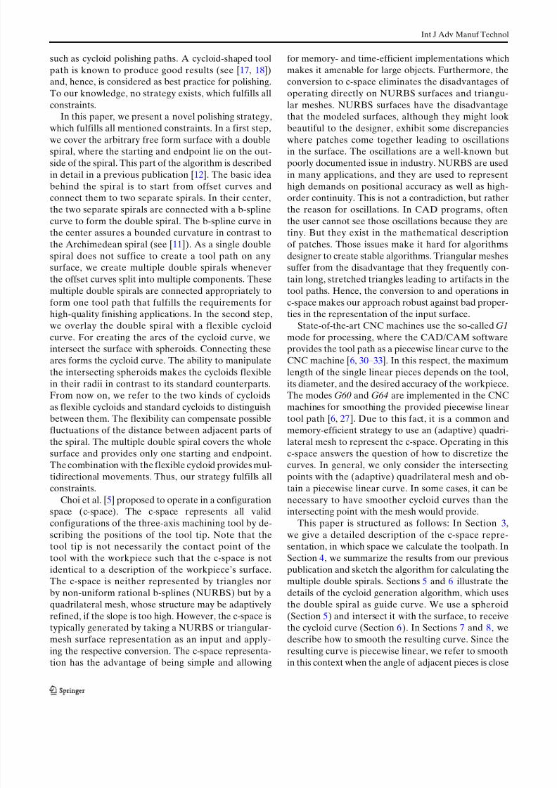
Choi et al. [5] proposed to operate in a configurationspace (c-space). The c-space represents all validconfigurations of the three-axis machining tool by de-scribing the positions of the tool tip. Note that thetool tip is not necessarily the contact point of thetool with the workpiece such that the c-space is notidentical to a description of the workpiece’s surface.The c-space is neither represented by triangles norby non-uniform rational b-splines (NURBS) but by aquadrilateral mesh, whose structure may be adaptivelyrefined, if the slope is too high. However, the c-space istypically generated by taking a NURBS or triangular-mesh surface representation as an input and apply-ing the respective conversion. The c-space representa-tion has the advantage of being simple and allowing

for memory- and time-efficient implementations whichmakes it amenable for large objects. Furthermore, theconversion to c-space eliminates the disadvantages of operating directly on NURBS surfaces and triangu-lar meshes. NURBS surfaces have the disadvantagethat the modeled surfaces, although they might lookbeautiful to the designer, exhibit some discrepancieswhere patches come together leading to oscillationsin the surface. The oscillations are a well-known butpoorly documented issue in industry. NURBS are usedin many applications, and they are used to representhigh demands on positional accuracy as well as high-order continuity. This is not a contradiction, but ratherthe reason for oscillations. In CAD programs, oftenthe user cannot see those oscillations because they aretiny. But they exist in the mathematical descriptionof patches. Those issues make it hard for algorithmsdesigner to create stable algorithms. Triangular meshessuffer from the disadvantage that they frequently con-tain long, stretched triangles leading to artifacts in thetool paths. Hence, the conversion to and operations inc-space makes our approach robust against bad proper-ties in the representation of the input surface.

State-of-the-art CNC machines use the so-called G1mode for processing, where the CAD/CAM softwareprovides the tool path as a piecewise linear curve to theCNC machine [6, 30–33]. In this respect, the maximumlength of the single linear pieces depends on the tool,its diameter, and the desired accuracy of the workpiece.The modes G60 and G64 are implemented in the CNCmachines for smoothing the provided piecewise lineartool path [6, 27]. Due to this fact, it is a common andmemory-efficient strategy to use an (adaptive) quadri-lateral mesh to represent the c-space. Operating in thisc-space answers the question of how to discretize thecurves. In general, we only consider the intersectingpoints with the (adaptive) quadrilateral mesh and ob-tain a piecewise linear curve. In some cases, it can benecessary to have smoother cycloid curves than theintersecting point with the mesh would provide.

This paper is structured as follows: In Section 3,we give a detailed description of the c-space repre-sentation, in which space we calculate the toolpath. InSection 4, we summarize the results from our previouspublication and sketch the algorithm for calculating themultiple double spirals. Sections 5 and 6 illustrate thedetails of the cycloid generation algorithm, which usesthe double spiral as guide curve. We use a spheroid(Section 5) and intersect it with the surface, to receivethe cycloid curve (Section 6). In Sections 7 and 8, wedescribe how to smooth the resulting curve. Since theresulting curve is piecewise linear, we refer to smoothin this context when the angle of adjacent pieces is close




workpiece

c-space

∆ z

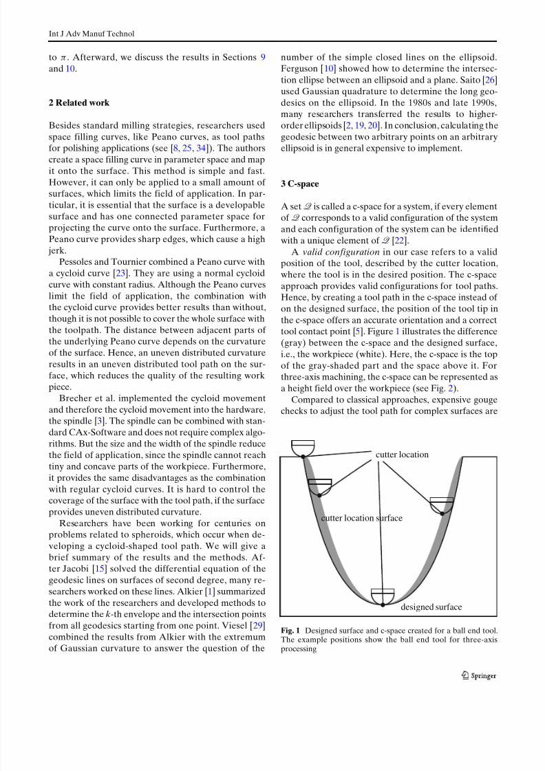
Fig. 2 The c-space (dashed line ) can be represented by a heightfield over the workpiece ( solid line )

obsolete. In Fig. 3, an example illustrates the benefit.Consider, in a first processing step, a tool is used witha large diameter, which cannot reach all parts of thesurface. Classical approaches withoutc-space create thetoolpath directly on the surface, which may lead tounreachable positions. This requires expensive correc-tions by gouge checking afterward.

One can create the c-space by discretizing—withrespect to the desired tolerance—the tooland thework-

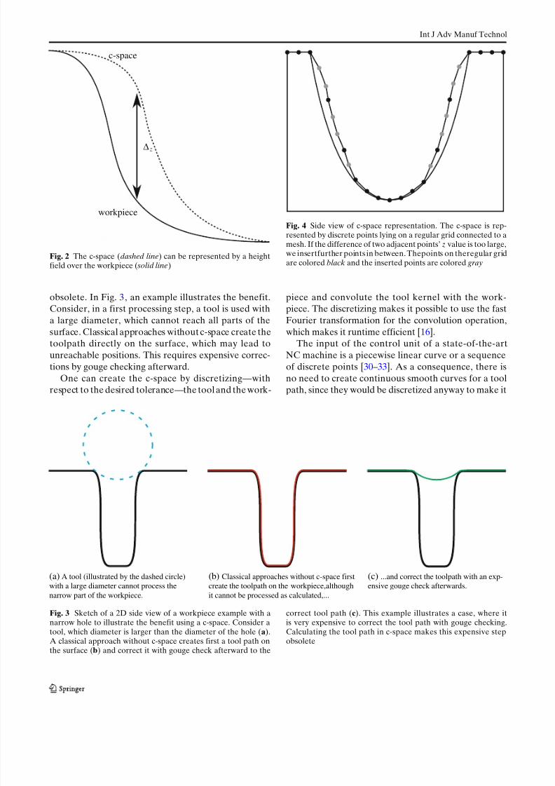
Fig. 4 Side view of c-space representation. The c-space is rep-resented by discrete points lying on a regular grid connected to amesh. If the difference of two adjacent points’ z value is too large,we insertfurther points in between.Thepoints on theregular gridare colored black and the inserted points are colored gray

piece and convolute the tool kernel with the work-piece. The discretizing makes it possible to use the fastFourier transformation for the convolution operation,which makes it runtime efficient [16].

The input of the control unit of a state-of-the-artNC machine is a piecewise linear curve or a sequenceof discrete points [30–33]. As a consequence, there isno need to create continuous smooth curves for a toolpath, since they would be discretized anyway to make it

(a) A tool (illustrated by the dashed circle)with a large diameter cannot process thenarrow part of the workpiece.

(b) Classical approaches without c-space firstcreate the toolpath on the workpiece,althoughit cannot be processed as calculated,...

(c) ...and correct the toolpath with an exp-ensive gouge check afterwards.

Fig. 3 Sketch of a 2D side view of a workpiece example with anarrow hole to illustrate the benefit using a c-space. Consider atool, which diameter is larger than the diameter of the hole (a).A classical approach without c-space creates first a tool path onthe surface (b) and correct it with gouge check afterward to the

correct tool path (c). This example illustrates a case, where itis very expensive to correct the tool path with gouge checking.Calculating the tool path in c-space makes this expensive stepobsolete




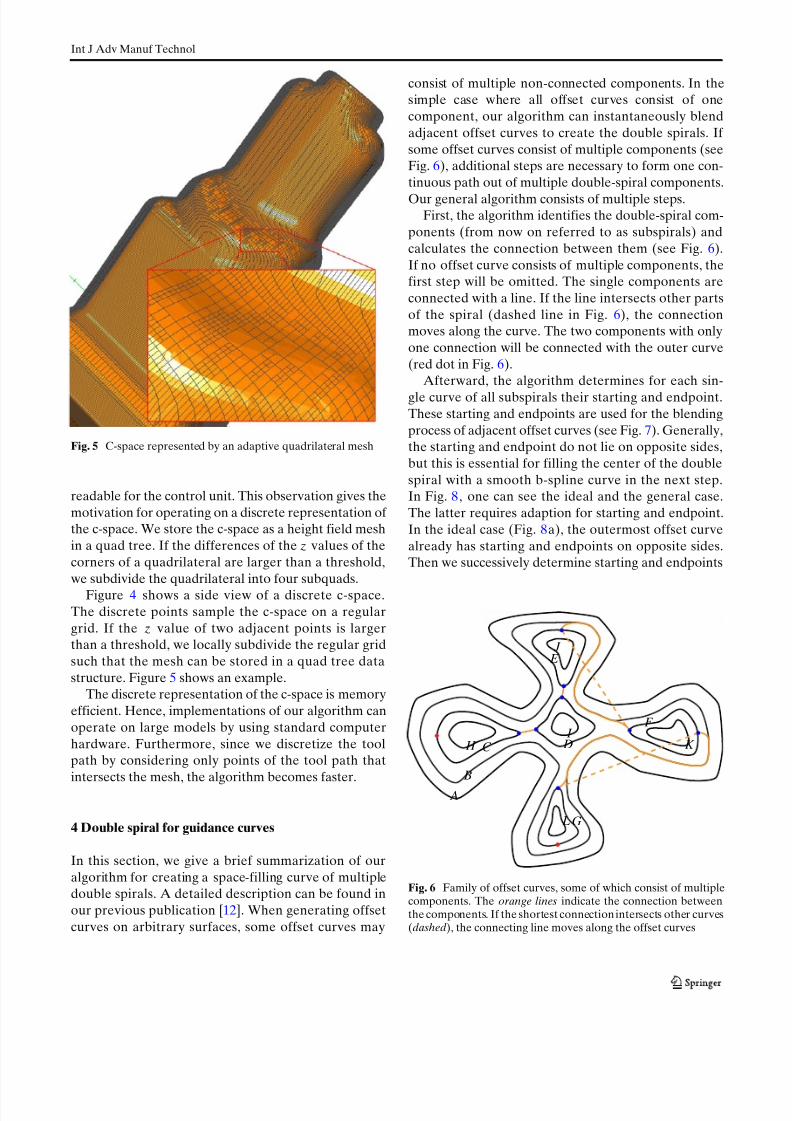
Fig. 5 C-space represented by an adaptive quadrilateral mesh

readable for the control unit. This observation gives themotivation for operating on a discrete representation of the c-space. We store the c-space as a height field meshin a quad tree. If the differences of the z values of thecorners of a quadrilateral are larger than a threshold,we subdivide the quadrilateral into four subquads.

Figure 4 shows a side view of a discrete c-space.The discrete points sample the c-space on a regulargrid. If the z value of two adjacent points is largerthan a threshold, we locally subdivide the regular gridsuch that the mesh can be stored in a quad tree datastructure. Figure 5 shows an example.

The discrete representation of the c-space is memoryefficient. Hence, implementations of our algorithm canoperate on large models by using standard computerhardware. Furthermore, since we discretize the toolpath by considering only points of the tool path thatintersects the mesh, the algorithm becomes faster.

4 Double spiral for guidance curves

In this section, we give a brief summarization of ouralgorithm for creating a space-filling curve of multipledouble spirals. A detailed description can be found inour previous publication [12]. When generating offsetcurves on arbitrary surfaces, some offset curves may

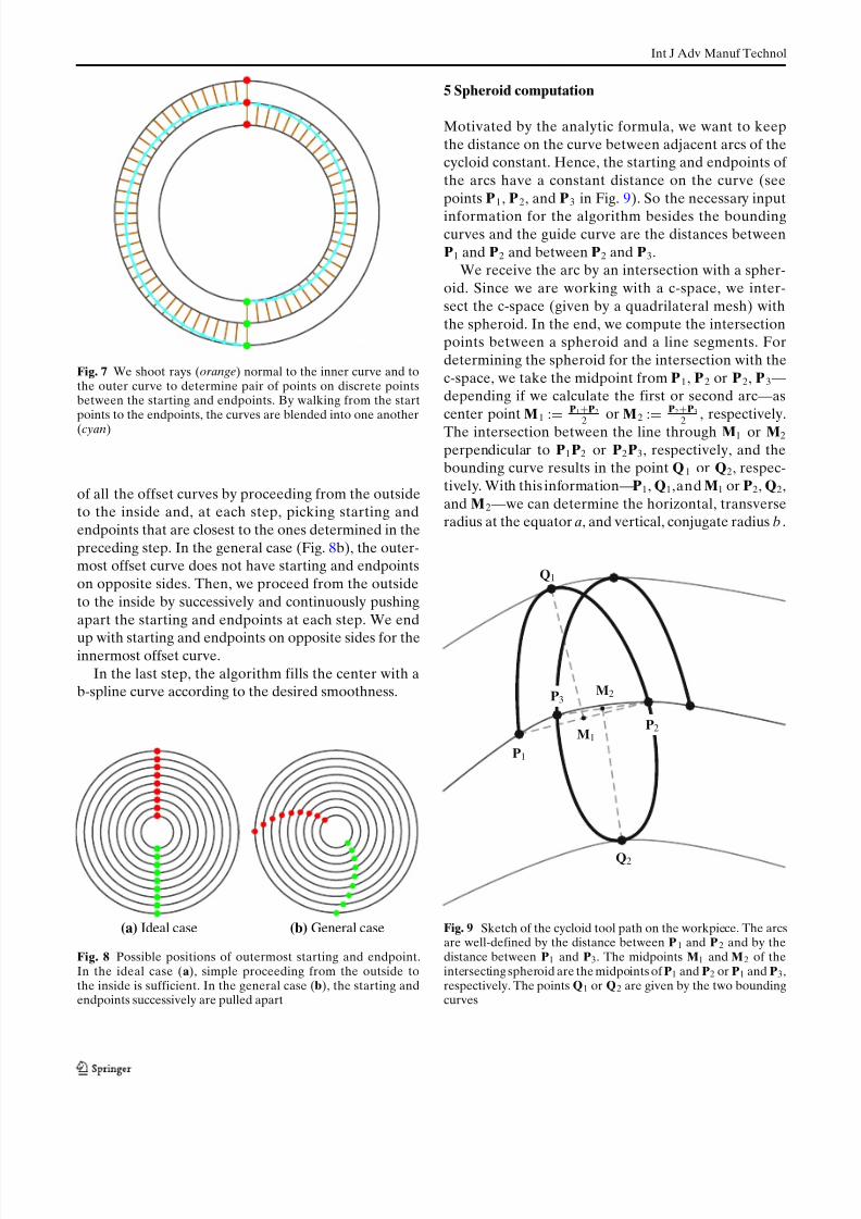
consist of multiple non-connected components. In thesimple case where all offset curves consist of onecomponent, our algorithm can instantaneously blendadjacent offset curves to create the double spirals. If some offset curves consist of multiple components (seeFig. 6), additional steps are necessary to form one con-tinuous path out of multiple double-spiral components.Our general algorithm consists of multiple steps.

First, the algorithm identifies the double-spiral com-ponents (from now on referred to as subspirals) andcalculates the connection between them (see Fig. 6).If no offset curve consists of multiple components, thefirst step will be omitted. The single components areconnected with a line. If the line intersects other partsof the spiral (dashed line in Fig. 6), the connectionmoves along the curve. The two components with onlyone connection will be connected with the outer curve(red dot in Fig. 6).

Afterward, the algorithm determines for each sin-gle curve of all subspirals their starting and endpoint.These starting and endpoints are used for the blendingprocess of adjacent offset curves (see Fig. 7). Generally,the starting and endpoint do not lie on opposite sides,but this is essential for filling the center of the doublespiral with a smooth b-spline curve in the next step.In Fig. 8, one can see the ideal and the general case.The latter requires adaption for starting and endpoint.In the ideal case (Fig. 8a), the outermost offset curvealready has starting and endpoints on opposite sides.Then we successively determine starting and endpoints

A

B

C D

E

F

G

H I

J

K

L

Fig. 6 Family of offset curves, some of which consist of multiplecomponents. The orange lines indicate the connection betweenthecomponents. If the shortest connectionintersects other curves(dashed ), the connecting line moves along the offset curves




Fig. 7 We shoot rays (orange ) normal to the inner curve and tothe outer curve to determine pair of points on discrete pointsbetween the starting and endpoints. By walking from the startpoints to the endpoints, the curves are blended into one another(cyan )

of all the offset curves by proceeding from the outsideto the inside and, at each step, picking starting andendpoints that are closest to the ones determined in thepreceding step. In the general case (Fig. 8b), the outer-most offset curve does not have starting and endpointson opposite sides. Then, we proceed from the outsideto the inside by successively and continuously pushingapart the starting and endpoints at each step. We end

up with starting and endpoints on opposite sides for theinnermost offset curve.In the last step, the algorithm fills the center with a

b-spline curve according to the desired smoothness.

(a) Ideal case (b) General case

Fig. 8 Possible positions of outermost starting and endpoint.In the ideal case (a), simple proceeding from the outside tothe inside is sufficient. In the general case (b), the starting andendpoints successively are pulled apart

5 Spheroid computation

Motivated by the analytic formula, we want to keepthe distance on the curve between adjacent arcs of thecycloid constant. Hence, the starting and endpoints of the arcs have a constant distance on the curve (seepoints P 1 , P 2, and P 3 in Fig. 9). So the necessary inputinformation for the algorithm besides the boundingcurves and the guide curve are the distances betweenP 1 and P 2 and between P 2 and P 3.

We receive the arc by an intersection with a spher-oid. Since we are working with a c-space, we inter-sect the c-space (given by a quadrilateral mesh) withthe spheroid. In the end, we compute the intersectionpoints between a spheroid and a line segments. Fordetermining the spheroid for the intersection with thec-space, we take the midpoint from P 1 , P 2 or P 2, P 3—depending if we calculate the first or second arc—ascenter point M 1 := P1 + P 2

2 or M 2 := P2 + P 32 , respectively.

The intersection between the line through M1 or M2

perpendicular to P1P 2 or P2P 3, respectively, and thebounding curve results in the point Q 1 or Q2, respec-tively. With this information—P 1, Q 1,and M1 or P 2, Q 2,and M 2—we can determine the horizontal, transverseradius at the equator a, and vertical, conjugate radius b .

Q 1

P 1

P 2

Q 2

P 3

M 1

M 2

Fig. 9 Sketch of the cycloid tool path on the workpiece. The arcsare well-defined by the distance between P 1 and P 2 and by thedistance between P1 and P3 . The midpoints M1 and M 2 of theintersectingspheroid are themidpointsof P 1 and P 2 or P 1 and P 3 ,respectively. The points Q 1 or Q 2 are given by the two boundingcurves




In the following, we show how to determine a and bfor the first arc. For the second arc, it is similar.

The implicit equation

xT A3x = 1, x ∈ R 3 (1)

with

A3 := a− 2

0 00 a− 2 00 0 b − 2

describes a spheroid with its center point in the originand its principal axes parallel to the x-, y-, and z-axes.A spheroid in arbitrary position can be described by theimplicit equation

xT T T RT y RT

z A 4 R z R yT x = 1, x ∈ P 3⊂ R 4 , (2)

where P 3 is the 3D projective space imbedded in R 4.Thus, the coordinates are given as homogenous coordi-

nates and

A4 :=

a− 2 0 0 00 a− 2 0 00 0 b − 2 00 0 0 1

.

The matrix T describes a translation and the matricesR y and R z describe a rotation around the y- and z-axis,respectively.

The center point and two points from the surface aresufficient for determining a and b . To make it simpler,we move the points so thatM1 is equal to the origin, and

afterward, we rotate the points so that M1Q 1 is parallelto ex, i.e., the x-axis. Basically, we reduce Eq. 2 to Eq. 1.Let

g := Q 1 − M1

and

gz :=1

g2 x + g2

y

g x, g y, 0 T ,

where g x and g y are the x- and the y-components of g.The sine and cosine of the angle α z for rotation around

the z-axis is determined bycos α z = gz, ex ,

= g x

g2 x + g2

y

,

sin(α z ) = 1 − cos 2 α z for g y ≥ 0,

− 1 − cos 2 α z otherwise.

Let gzx := Rz (g) and gzx0 its normalized vector. Afterdetermining the angles between gzx0 and ex, sine andcosine of all angles are determined. The sine and cosinefor rotation around the y-axis can be determined in asimilar way by

cos α y = gzx0 , ex ,

sin α y = 1 − cos 2 α y for gzx z ≥ 0,

− 1 − cos 2 α y otherwise,

where gzx z is the z-component of gzx.With

u := R y R z q1 − m1 ,

v := R y R z p1 − m1

the values a and b can be determined by

b = u2 xv2

y + u2 xv2

z − u2 yv2

x −u2

z v2 x

u2 x

− v2 x, , (3)

= u xv y, (4)

a = b 2u2 x

b 2 − u2 y − u2

z, (5)

= u x. (6)

The rotation of Q1 − M1 and P1 − M1 by R y R z

causes u to be parallel to the x-axis and v to be parallelto the y-axis. Hence, the denominator in Eqs. 3 and 5is always non-zero, and therefore, these equation canalways be solved.

6 Cycloid computation

The c-space is given by a mesh. Hence, the points fromthe tool path are the intersection points between the c-space and the spheroid. Basically we have to intersectthe spheroid with a line to determine the points. To

simplify the computation of the intersection points, wemove and rotate everything, such that the center of the spheroid is in the origin and the principal axes areparallel to the x-, y-, and z-axes (see Section 5).

Let the spheroid be given by a and b and the linegiven by x1 + sx2. The intersecting points result fromsolving

x1 + sx2T A x1 + sx2 = 1




with respect to s. Let

a :=b 2

a2

a2,

m a := a , x2 ,

mb := 2 a , x1 ,

m c := a , x1 − a2b 2 ,

d := m2b − 4m a m c

then

s = mb ± d

2m a.

7 Elliptic arc representation

The resulting arcs are computed in form of discreterepresentations. If the resulting arcs have the shape of a “flattened” ellipse rather than a circle, the discreterepresentation may lead to a rather jagged tool pathinstead of a smooth one. A solution for this problemis to refine the mesh. Refining is an expensive strategybecause it increases the calculation time for all algo-rithms and increases the memory usage. So it is a betterstrategy to refine the arc representation and insert arcpoints in the interior of the quads, if the arc’s curvatureexceeds a curvature threshold. In our experiments, weachieved good results by refining the representation,when the absolute cosine of the enclosed angle of adjacent parts is smaller than0.995 . We use the cosine ascriteria, since it is cheap to compute it with the scalarproduct.

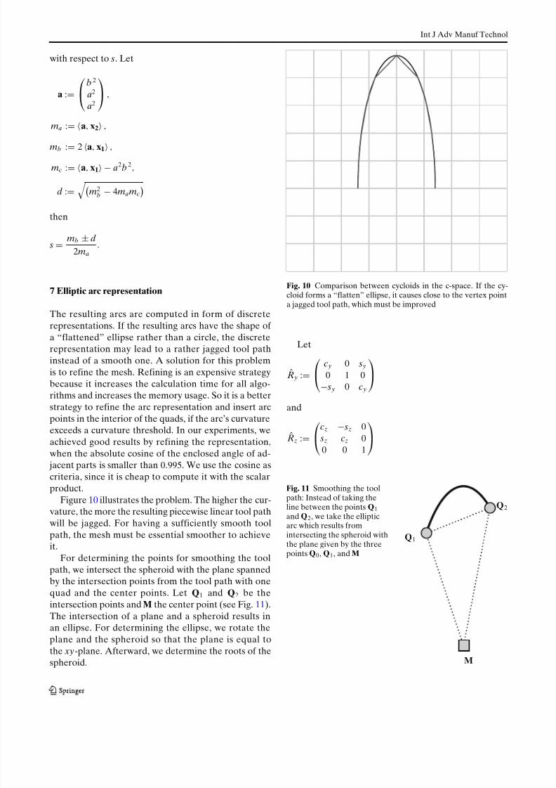
Figure 10 illustrates the problem. The higher the cur-vature, the more the resulting piecewise linear tool pathwill be jagged. For having a sufficiently smooth toolpath, the mesh must be essential smoother to achieveit.

For determining the points for smoothing the toolpath, we intersect the spheroid with the plane spannedby the intersection points from the tool path with onequad and the center points. Let Q1 and Q2 be theintersection points and M the center point (see Fig. 11).The intersection of a plane and a spheroid results inan ellipse. For determining the ellipse, we rotate theplane and the spheroid so that the plane is equal tothe xy-plane. Afterward, we determine the roots of thespheroid.

Fig. 10 Comparison between cycloids in the c-space. If the cy-cloid forms a “flatten” ellipse, it causes close to the vertex pointa jagged tool path, which must be improved

Let

R y :=c y 0 s y0 1 0

− s y 0 c y

and

R z :=cz − sz 0 sz cz 00 0 1

Fig. 11 Smoothing the toolpath: Instead of taking theline between the points Q 1and Q 2 , we take the ellipticarc which results fromintersecting the spheroid withthe plane given by the threepoints Q 0 , Q 1 , and M

Q 1

Q 2

M




with s y := sin(β y), c y := cos (β y), sz := sin(β z ), and cz :=cos (β z ) be the rotation matrices, which rotate the inter-secting plane into the xy-plane. With

B := R T y

R T z A 3 R z R y

=

c yc2z + c1 s2

z

a2 c1 0c yc2

z + c y s2z

a2 s y − s yc y

b 2

0 s2z + c

2z

a2 0

s yc2z + s y s2

z

a2 c1 − s yc y

b 2 0 s yc2

y + s y s2z

a2 s y +c2 y

b 2

the rotated spheroid can be described by

xT Bx = 1.

Now, all the points on the spheroid which lie in the xy-plane are the points on the desired ellipse. Insert-ing xz0 := ( x, y, 0)T in the equation above gives us theformula for the ellipse

xT z0 Bxz0 = x2c2

yc2

z + c2

y s2

za2 +

s2

yb 2 + y2 s

2z + c

2z

a2 .

With

a :=c2

yc2z + c2

y s2z

a2 +

s2 y

b 2

− 1

b := a2

s2z + c2

z

the derived ellipse is given by

x2

a2 + y

2

b 2= 1.

Converting the arc of the ellipse into rational Bézierrepresentation provides the opportunity to use a sub-division algorithm to get sufficiently many points, suchthat the resulting piecewise linear curve will not have a“flattened” shape.

8 Rational Bezier representation

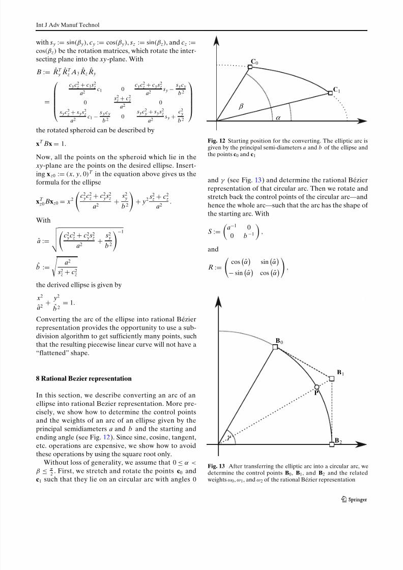
In this section, we describe converting an arc of anellipse into rational Bezier representation. More pre-cisely, we show how to determine the control pointsand the weights of an arc of an ellipse given by theprincipal semidiameters a and b and the starting andending angle (see Fig. 12). Since sine, cosine, tangent,etc. operations are expensive, we show how to avoidthese operations by using the square root only.

Without loss of generality, we assume that0 ≤ α <β ≤ π

2 . First, we stretch and rotate the points c0 andc1 such that they lie on an circular arc with angles0

C 0

C 1

α

β

Fig. 12 Starting position for the converting. The elliptic arc isgiven by the principal semi-diameters a and b of the ellipse andthe points c0 and c1

and γ (see Fig. 13) and determine the rational Bézierrepresentation of that circular arc. Then we rotate and

stretch back the control points of the circular arc—andhence the whole arc—such that the arc has the shape of the starting arc. With

S := a− 1 00 b − 1 ,

and

R :=cos α sin α

− sin α cos α,

γ

B 0

B 1

B 2

P

Fig. 13 After transferring the elliptic arc into a circular arc, wedetermine the control points B0 , B1 , and B2 and the relatedweights ω0 , ω1 , and ω2 of the rational Bézier representation




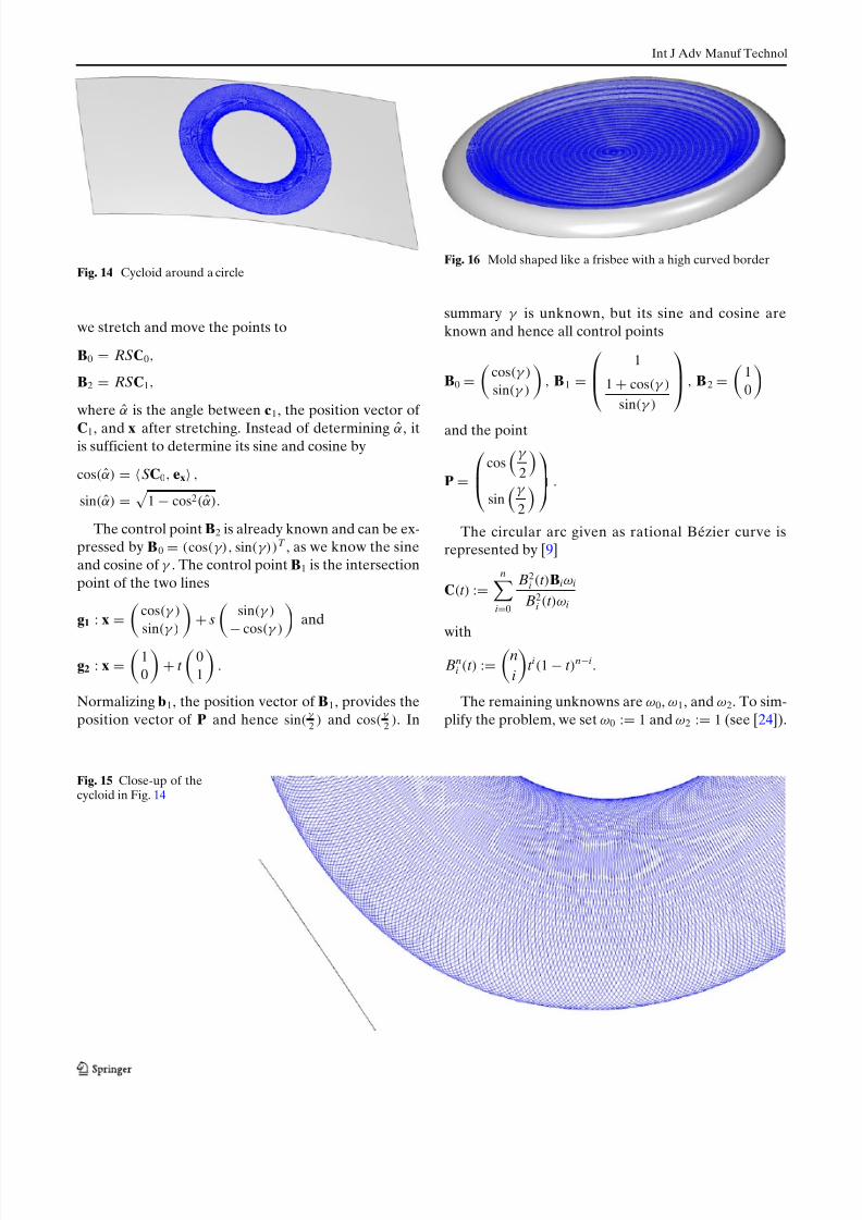
Fig. 14 Cycloid around a circle

we stretch and move the points to

B0 = RSC0 ,

B2 = RSC1 ,

where α is the angle between c1, the position vector of C1, and x after stretching. Instead of determining α , itis sufficient to determine its sine and cosine by

cos (α) = SC0 , ex ,

sin(α) = 1 − cos 2(α).

The control point B2 is already known and can be ex-pressed by B0 = (cos (γ), sin(γ)) T , as we know the sineand cosine of γ . The control point B1 is the intersectionpoint of the two lines

g1 : x =cos (γ )sin(γ )

+ ssin(γ )

− cos (γ ) and

g2 : x = 10

+ t 01

.

Normalizing b1, the position vector of B1 , provides theposition vector of P and hence sin( γ

2 ) and cos ( γ 2 ). In

Fig. 16 Mold shaped like a frisbee with a high curved border

summary γ is unknown, but its sine and cosine areknown and hence all control points

B0 =cos (γ )sin(γ )

, B1 =1

1 + cos (γ )sin(γ )

, B 2 =10

and the point

P =cos

γ 2

sinγ 2

.

The circular arc given as rational Bézier curve isrepresented by [9]

C(t ) :=n

i= 0

B2i (t )B iω i

B2i (t )ω i

with

Bni (t ) :=

ni

t i(1 − t )n− i .

The remaining unknowns are ω0, ω1, and ω2. To sim-plify the problem, we set ω0 := 1 and ω2 := 1 (see [24]).

Fig. 15 Close-up of thecycloid in Fig. 14




Fig. 17 Close up of Fig. 16

The remaining unknown is ω1. Although the parame-trization is not the natural parametrization, we knowfrom the deCasteljau-Algorithm [9] that C(0.5) = P ,with P = (cos ( γ

2 ), sin( γ 2 )) T . By solving the equation

C(0.5) = P for ω1, we receive

ω1 =12

1 + cos (γ ) − 2 cos γ 2

− 1 + cos γ 2

.

Applying the two affine transformations, rotation by

R− 1 =cos α − sin α

sin α cos α,

and stretching by

S− 1 = a 00 b

,

to the control points B i, we receive the desired controlpoints of the elliptic arc.

9 Results and discussion

We developed and implemented the algorithm for cre-ating cycloid curves around a given guide curve. All thecalculating and simulating steps were executed on a PCwith an Intel(R) Core(TM) Duo CPU with 2.2 GHz,3 GB of RAM with Windows Vista as operating system.

The algorithm has only two input parameters: First,the distance between adjacent parts of the spiral curve.Since the spiral is created from offset curves, this pa-rameter refers to the offset. Second, the density of the cycloids. This results in the distance between P1

and P2 and between P2 and P3 shown in Fig. 9. Ourexperiments showed that the first parameter—theoffset parameter—should be chosen in a way that thecurvature circle of the resulting cycloid curves is sig-nificantly smaller than the curvature circle of the multi-ple double-spiral curve. Otherwise, it may possible thatthe surface is not completely covered by the toolpath.

Figures 14 and 15 show a cycloid around a circle ona curved surface. Here the inputs are three interleavedcircles, where the outer and the inner circle bound thecycloid, while the middle circle is the guide curve. Thiscycloid curve contains 643 arcs and was computed inless than a second. The computation time does notinclude the time for creating the c-space.

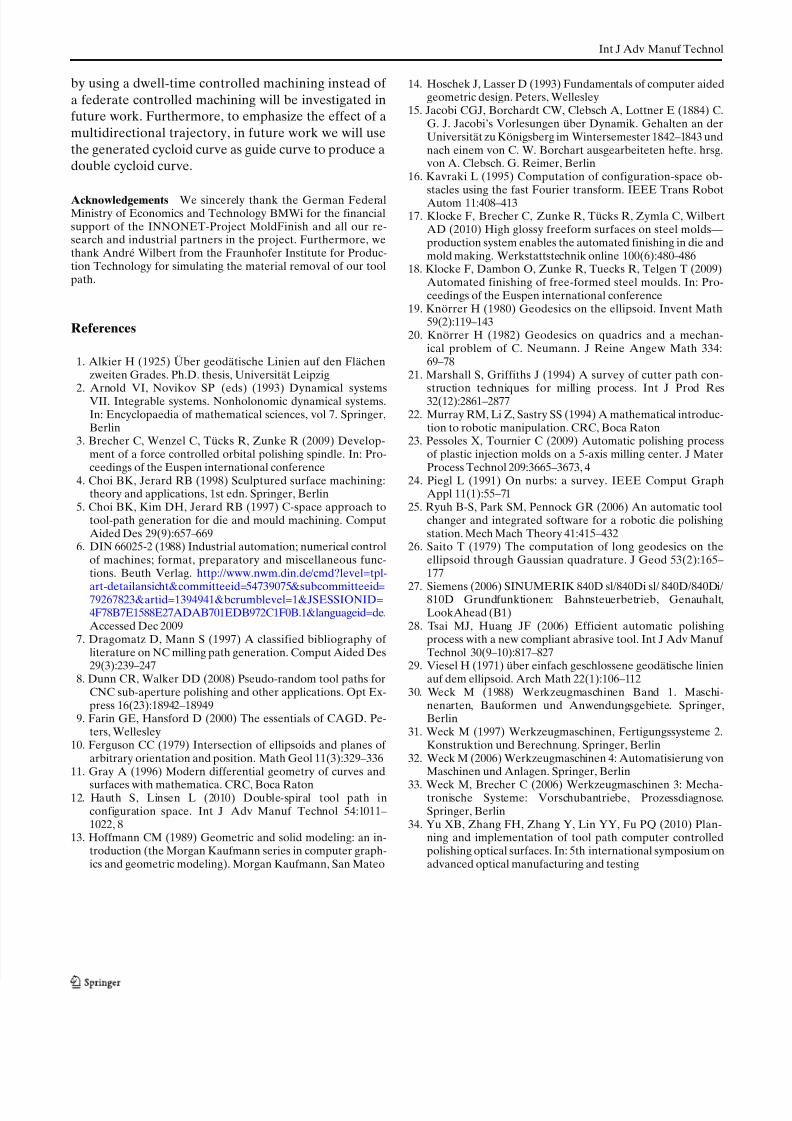
Figures 16, 17, and 18 show an example, where adouble spiral is used as guide and as bounding curve.When using a double-spiral curve as a guide and asa bounding curve, we use Q i :=

12 (Q i − Mi) + Mi for

i ∈ {1, 2} instead of Q1 and Q2 for generation of thecycloid curves (according to Fig. 9). The result is aspace filling cycloid curve. The cycloid in this examplecontains 14,804 arcs and was computed in 10.2 s. Herethe computation time also does not include the time forcreating the c-space and the time for creating the spiral.

Fig. 18 Another close up of Fig. 16




Fig. 19 This figure shows the resulting cycloid curve. Here, thecycloid curve covers the whole surfaces

In Figs. 19 and 20, we present a third example, wherewe used also a spiral curve (see Fig. 21) as guide aswell as bounding curve, which results in a space fillingcycloid curve. This example contains 15,604 arcs of thecycloid and was computed in 11.8 s. Here the computa-tion time also does not include the time for creating thec-space and the time for creating the spiral.

All examples show that the cycloid curve alwaystouches the border and never crosses or misses the

Fig. 21 We use the spiral curve as the guide curve for our cycloidalgorithm. By using this curve, the resulting cycloid curve will bea space filling curve

border. This provides an advantage compared withstandard cycloid curves discussed in literature or cy-cloids created by the spindle, since one can control themachined area. In addition, one can control severalparameters, like the density of the flexible cycloids.Due to the fast computation time, this method providesa cheap and better alternative solution compared to animplementation of the cycloid by the spindle.

Fig. 20 Close up of thecycloid curve




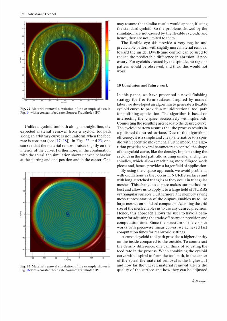
Fig. 22 Material removal simulation of the example shown inFig. 14 with a constant feed rate. Source: Fraunhofer IPT

Unlike a cycloid toolpath along a straight line, theexpected material removal from a cycloid toolpathalong an arbitrary curve is not uniform, when the feedrate is constant (see [17, 18]). In Figs. 22 and 23, onecan see that the material removal raises slightly on theinterior of the curve. Furthermore, in the combinationwith the spiral, the simulation shows uneven behaviorat the starting and end-position and in the center. One

Fig. 23 Material removal simulation of the example shown inFig. 16 with a constant feed rate. Source: Fraunhofer IPT

may assume that similar results would appear, if usingthe standard cycloid. So the problems showed by thesimulation are not caused by the flexible cycloids, andhence, they are not limited to them.

The flexible cycloids provide a very regular andpredictable pattern with slightly more material removaltoward the inside. Dwell-time control can be used toreduce the predictable difference in abrasion, if nec-essary. For cycloids created by the spindle, no regularpattern would be observed, and thus, this would notwork.

10 Conclusion and future work

In this paper, we have presented a novel finishingstrategy for free-form surfaces. Inspired by manuallabor, we developed an algorithm to generate a flexiblecycloid curve to provide a multidirectional tool pathfor polishing application. The algorithm is based onintersecting the c-space successively with spheroids.Connecting the resulting arcs leads to the desired curve.The cycloid pattern assures that the process results ina polished deburred surface. Due to the algorithmsefficiency, it is a simple and cheap alternative to a spin-dle with eccentric movement. Furthermore, the algo-rithm provides several parameters to control the shapeof the cycloid curve, like the density. Implementing thecycloids in the tool path allows using smaller and lighterspindles, which allows machining more filigree workpieces and, hence, provides a larger field of application.

By using the c-space approach, we avoid problemswith oscillations as they occur in NURBS surfaces andwith long, stretched triangles as they occur in triangularmeshes. This change to c-space makes our method ro-bust and allows us to apply it to a large field of NURBSor triangular surfaces. Furthermore, the memory savingmesh representation of the c-space enables us to uselarge meshes on standard computers. Adapting the gridsize of the mesh enables us to use any desired precision.Hence, this approach allows the user to have a para-meter for adjusting the trade-off between precision andcomputation time. Since the structure of the c-spaceworks with piecewise linear curves, we achieved fastcomputation times for real-world settings.

A curved cycloid tool path provides a higher densityon the inside compared to the outside. To counteractthe density difference, one can think of adjusting thefeed rate in the process. When combining the cycloidcurve with a spiral to form the tool path, in the centerof the spiral the material removal is the highest. If and how far the uneven material removal affects thequality of the surface and how they can be adjusted




by using a dwell-time controlled machining instead of a federate controlled machining will be investigated infuture work. Furthermore, to emphasize the effect of amultidirectional trajectory, in future work we will usethe generated cycloid curve as guide curve to produce adouble cycloid curve.

Acknowledgements We sincerely thank the German FederalMinistry of Economics and Technology BMWi for the financialsupport of the INNONET-Project MoldFinish and all our re-search and industrial partners in the project. Furthermore, wethank André Wilbert from the Fraunhofer Institute for Produc-tion Technology for simulating the material removal of our toolpath.

References

1. Alkier H (1925) Über geodätische Linien auf den Flächenzweiten Grades. Ph.D. thesis, Universität Leipzig

2. Arnold VI, Novikov SP (eds) (1993) Dynamical systemsVII. Integrable systems. Nonholonomic dynamical systems.In: Encyclopaedia of mathematical sciences, vol 7. Springer,Berlin

3. Brecher C, Wenzel C, Tücks R, Zunke R (2009) Develop-ment of a force controlled orbital polishing spindle. In: Pro-ceedings of the Euspen international conference

4. Choi BK, Jerard RB (1998) Sculptured surface machining:theory and applications, 1st edn. Springer, Berlin

5. Choi BK, Kim DH, Jerard RB (1997) C-space approach totool-path generation for die and mould machining. ComputAided Des 29(9):657–669

6. DIN 66025-2 (1988) Industrial automation; numerical controlof machines; format, preparatory and miscellaneous func-tions. Beuth Verlag. http://www.nwm.din.de/cmd?level=tpl-

art-detailansicht&committeeid=54739075&subcommitteeid=79267823&artid=1394941&bcrumblevel=1&JSESSIONID=4F78B7E1588E27ADAB701EDB972C1F0B.1&languageid=de.Accessed Dec 2009

7. Dragomatz D, Mann S (1997) A classified bibliography of literature on NC milling path generation. Comput Aided Des29(3):239–247

8. Dunn CR, Walker DD (2008) Pseudo-random tool paths forCNC sub-aperture polishing and other applications. Opt Ex-press 16(23):18942–18949

9. Farin GE, Hansford D (2000) The essentials of CAGD. Pe-ters, Wellesley

10. Ferguson CC (1979) Intersection of ellipsoids and planes of arbitrary orientation and position. Math Geol 11(3):329–336

11. Gray A (1996) Modern differential geometry of curves and

surfaces with mathematica. CRC, Boca Raton12. Hauth S, Linsen L (2010) Double-spiral tool path inconfiguration space. Int J Adv Manuf Technol 54:1011–1022, 8

13. Hoffmann CM (1989) Geometric and solid modeling: an in-troduction (the Morgan Kaufmann series in computer graph-ics and geometric modeling). Morgan Kaufmann, San Mateo

14. Hoschek J, Lasser D (1993) Fundamentals of computer aidedgeometric design. Peters, Wellesley

15. Jacobi CGJ, Borchardt CW, Clebsch A, Lottner E (1884) C.G. J. Jacobi’s Vorlesungen über Dynamik. Gehalten an derUniversität zu Königsberg im Wintersemester 1842–1843 undnach einem von C. W. Borchart ausgearbeiteten hefte. hrsg.von A. Clebsch. G. Reimer, Berlin

16. Kavraki L (1995) Computation of configuration-space ob-stacles using the fast Fourier transform. IEEE Trans RobotAutom 11:408–413

17. Klocke F, Brecher C, Zunke R, Tücks R, Zymla C, WilbertAD (2010) High glossy freeform surfaces on steel molds—production system enables the automated finishing in die andmold making. Werkstattstechnik online 100(6):480–486

18. Klocke F, Dambon O, Zunke R, Tuecks R, Telgen T (2009)Automated finishing of free-formed steel moulds. In: Pro-ceedings of the Euspen international conference

19. Knörrer H (1980) Geodesics on the ellipsoid. Invent Math59(2):119–143

20. Knörrer H (1982) Geodesics on quadrics and a mechan-ical problem of C. Neumann. J Reine Angew Math 334:69–78

21. Marshall S, Griffiths J (1994) A survey of cutter path con-

struction techniques for milling process. Int J Prod Res32(12):2861–287722. Murray RM, Li Z, Sastry SS (1994) A mathematical introduc-

tion to robotic manipulation. CRC, Boca Raton23. Pessoles X, Tournier C (2009) Automatic polishing process

of plastic injection molds on a 5-axis milling center. J MaterProcess Technol 209:3665–3673, 4

24. Piegl L (1991) On nurbs: a survey. IEEE Comput GraphAppl 11(1):55–71

25. Ryuh B-S, Park SM, Pennock GR (2006) An automatic toolchanger and integrated software for a robotic die polishingstation. Mech Mach Theory 41:415–432

26. Saito T (1979) The computation of long geodesics on theellipsoid through Gaussian quadrature. J Geod 53(2):165–177

27. Siemens (2006) SINUMERIK 840D sl/840Di sl/ 840D/840Di/810D Grundfunktionen: Bahnsteuerbetrieb, Genauhalt,LookAhead (B1)

28. Tsai MJ, Huang JF (2006) Efficient automatic polishingprocess with a new compliant abrasive tool. Int J Adv Manuf Technol 30(9–10):817–827

29. Viesel H (1971) über einfach geschlossene geodätische linienauf dem ellipsoid. Arch Math 22(1):106–112

30. Weck M (1988) Werkzeugmaschinen Band 1. Maschi-nenarten, Bauformen und Anwendungsgebiete. Springer,Berlin

31. Weck M (1997) Werkzeugmaschinen, Fertigungssysteme 2.Konstruktion und Berechnung. Springer, Berlin

32. Weck M (2006) Werkzeugmaschinen 4: Automatisierung vonMaschinen und Anlagen. Springer, Berlin

33. Weck M, Brecher C (2006) Werkzeugmaschinen 3: Mecha-tronische Systeme: Vorschubantriebe, Prozessdiagnose.Springer, Berlin

34. Yu XB, Zhang FH, Zhang Y, Lin YY, Fu PQ (2010) Plan-ning and implementation of tool path computer controlledpolishing optical surfaces. In: 5th international symposium onadvanced optical manufacturing and testing

http://www.nwm.din.de/cmd?level=tpl-art-detailansicht&committeeid=54739075&subcommitteeid=79267823&artid=1394941&bcrumblevel=1&JSESSIONID=4F78B7E1588E27ADAB701EDB972C1F0B.1&languageid=de









Hauth 2011 Cycloid

Documents

Transcript of Hauth 2011 Cycloid