Harrod's Model ofGrowth Cycle A Note - CORE · Harrod's Model ofGrowth Cycle A Note TakaoFujimoto...

Harrod's Model of Growth Cycle A Note

Takao Fujimoto

Yasuhiko Namba

1. Introduction

In Harrod (1939), we can read the following paragraph:

"Space forbids an application of this method of analysis to the successive

phases of the trade cycle. In the course of it the values expressed by the

symbols on the right-hand side of the equation undergo considerable

change. As actual growth departs upwards or downwards from the war

ranted level, the warranted rate itself moves, and may chase the actual

rate in either direction. (Harrod (1939), pp.28-29).

Fujimoto (1994) presented a simple model in which the number of

equilibrium relations assumed, explicit or implicit, are kept to the mini

mum, and showed that instability persists. In the model, the capital coef

ficient and the desired saving ratio are constant. Then Kominami (1995)

worked out a numerical example in which a simple model a la Harrod dis

plays cyclical movements, making the desired saving ratio variable

through time. Recently Namba(1995) showed the instability of equilib

rium growth in a model which incorporates micro-foundations for some of

macro relations together with the price level, the wage rate and the profit

rate.

The purpose of this note is to reformulate Fujimoto's model with the

-365-

1110

desired saving ratio being variable, and conduct a preliminary study of

simulations.

2. A Simple Model

The symbols we emply are:

y~ : expected or normal gross output at the beginning of period t.

Y, : actual gross output at the period t.

K, : capital stock at the beginning of period t.

8 : rate of depreciation of capital stock( assumed to be constant).

C* : desired capital-output ratio (assumed to be constant).

g~ : desired rate of accumulation ofK at the beginning ofperiod t.

g, : actual rate of accumulation at the period t.

r: :desired gross investment at the beginning ofperiod t.

I, : actual gross investment at the period t.

D~ : expected demand for goods and services at the period t.

s; : desired (gross) saving ratio at the period t.

s, : actual (gross) saving ratio at the period t.

u, : degree of utilization ofcapital stock at the period t.

In the below, subscript t will be dropped when the explanation is about a

period in general. Note that the rate of accumulation is used in the gross

sense, and the terms expected and desired are loosely interchangeable.

Now suppose at the beginning of period t, the magnitudes K, ge, and

s' are given. The expected gross investment is determined by

Ie =geK.

The expected gross output is

ye = KjC'

-366-

(2)

Harrod's Model of Growth Cycle: A Note 1111

The scheduled demand is then given as

De = (1 - s*)ye +Ie.

We now make the assumption that

Y = midi (ye, De).

(3)

(4)

The mid (x,y) function returns a value which is an intermediate point on

the segment between x and y. (See Fujimoto (1994) for more explanation.)

Below this type of function shall be called a mid function. The degree of

utilization of capital stock u is measured by

u = yjye.

The actual gross investment is determined by

1= mid2 (Ie, s'Ye).

The function mid2 (".) is another mid function. Note here that

(5)

(6)

r > s*ye ifand only if De> yeo

From the ex post identity, the actual gross accumulation rate and saving

ratio can be calculated as

g =I/K. and

s =I/Y.

Eq.(l) is a modified version of accelerator principle, while eq.(6) is a

modified multiplier principle. In the literature published so far, it has

been normally assumed that the expected investment is realized. The

above equations determines all the variables at the period t. The dynamic

equations are described by the following.

(

Kt+1 = K,(1 - 8) + I"

g~+1 =g~ +flu"~ D~/y~), and

S;+I = mid3 (s;, s) +a' (g, - g~).

Here the function flu, v) is such that it is defined on the set

{(u, v) I u, v 2 1 or 1 2 u, v 20},

-367-

1112

flI, 1) = 0 and is non-decreasing in each variable. The coefficient a in the

last equation ofthe adjustment system is a given positive constant.

First note that the above model has the warranted rate of gross accu

mulation at the perios t, g7 == s7 IC. If g~ = g7, this rate g7 and s7 will per

sist into the future, and each expected rate is realized with u, =1. The ac

tual rate of growth in gross output and that of capital stock are the same

and equal to g7 - 8. The intrinsic instability of the model was shown in

Fujimoto(1994) provided the desired saving ratio remains constant. What

will happen if the desired saving ratio is allowed to change, and the war

ranted rate is set to chase the actual rate of accumulation? In this note we

present some results obtained in simulation studies on a personal com

puter.

3. A Simulation

To render our model still more tractable, we take up a simplest form

of mid functions. The functions used are:

midi (x,y) = mi' x+ (1 - mi) 'y,

where mi is a given positive constant coefficient(less than one) in each mid

function. We also take up a simple form for the function flu, v) :

flu,v)=aI'(u-I)+a2'(v-I),

where aI, and a2 are fixed positive constants.

We also put the upper and lower limits for the planned rate of accu

mulation ge. This rate ge has to be in a given segment [gmin,gmax]' In Fig.I,

a result is shown. The constants are:

C* = 3.0, 8 = 0.0125, gmax = 0.08, gmin = -0.05,

ml =0.5, m2=0.5, m3=0.5, aI=0.2, a2=0.1, a=0.5,

-368-


The initial values are:

Ko =10.0, go =0.05, So *=0.12.

After all these complications, the instability still survive. To have cy

clical movements, the desired saving ratio should be allowed to vary more

wildly. So, the adjustment equation for s; is revised as :

S;+1 = mid3 (s;'s,) +a' gr. (7)

Thus, there is no longer the warranted rate as defined by Harrod.

In Fig.l, the darker cyclical curve in the middle shows the series of

the annual gross output Yr' The less darker curve nearby is the series of

Y~. From Fig. 1, we can see the model displays a fairly regular cycles of pe

riod 25 years or so. This period is not very different from the period found

in the simulation studies of Goodwin's growth cycle model.

(The program for simulation is written in Visual Basic(Microsoft Corp.)

ver.1.0, and given in Appendices. This program can be run on Visual Basic

ver.2.0 up to ver.4.0 without modification, with suitable forms defined.)

4. Remarks

In Fig.2, another simulation result is presented. This is obtained by

reducing the depreciation rate from 0.0125 to 0.005. The model economy

has expanded and got out ofthe window. The same result can be obtained

if we raise the minimun accumulation rate from -0.05 to -0.03, while

keeping the depreciation rate fixed at 0.0125.

Fig.3 tells us that the period of cycles can be changed drastically by

modifying the coefficients mi' In the result shown in Fig.3, we modified

as:

m3 =0.85, and gmin =- 0.04.

-369-

1114

The fact that m3 is nearer to unity implies that in revising the desired sav

ing ratio, the actual accumulation rate has less influence. Fig.3 realizes a

period as long as 50 years, which is comparable to Condratiev cycles.

One may make the desired capital-output ratio variable as time goes

on. And eq.(2) is a little awkward in the presence of continuous over- or

under utilization of capital. More importantly, eq.(7) is rather ad hoc, and

excludes the existence of the warranted rate of growth. This should be

modified. For example, we include the natural rate of growth, g", to refor

mulate eq.(7) :

S;+I = mid3 (s; ,s,) +a' (g, - gO). (8)

Now the system has the balanced growth at the warranted rate,

g~ = s; IC*, provided that this warranted rate is equal to the natural rate.

That the natural rate plays a substantial role in the short-run also is not

unrealistic. Since we have adopted simple linear mid functions, the for

mulation is not different from simple linear adaptive adjustment. So we

may try

S;+I =s; + b' (s, - s;), (9)

where b is now allowed to be greater than unity.

One more problem to tackle with is the non-negativity ofvariouscoef

ficients, to which we paid no attention while Harrod (1939) was careful

enough on this matter.

In our next paper, we will consider the above points as well as the

economic meanings of changes in various parameters, and also the impli

cations of government intervention through public spending after incorpo

rating Harrods idea on this point.

Our tentative conclusion in this simulation study is that persuing

Harrods ideas to create trade cycles with a variable desired saving ratio

-370-


may not be successful: a new twist seems necessary as can be seen in eqs.

(7)-(9). A variable desired capital-output ratio may be of help.

References

Fujimoto, T.(1994): Harrodian Instability Principle in Full Disequilibrium, Okayama

Economic Review, Vol.25(4), pp.154-164.

Harrod, R.F. (1939): An Essay in Dynamic Theory, Economic Journal, Vol. 49, pp.l4

33.

Kominami, Atsuko (1995): A Study on Harrod's Instability Principle (in Japanese),

MA Thesis (Dept. ofEcon., Univ. of Okayama).

Namba, Y. (1995): On the Instability of Equilibrium Growth (in Japanese), Studies in

Contemporary Economics (Western Association of Economics), VolA, ppA3-57.

-371-

1116

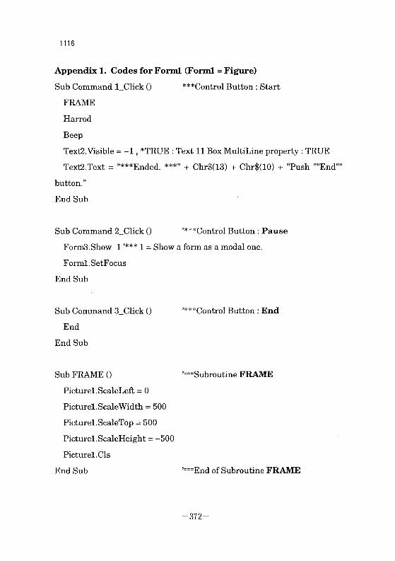
Appendix 1. Codes for Forml (Forml =Figure)

Sub Command CClick 0 ***Control Button: Start

FRAME

Harrod

Beep

Text2.Visible =-1, *TRUE : Text 11 Box MultiLine property: TRUE

Text2.Text = "***Ended. ***" + Chr$(13) + Chr$(10) + "Push ''''End''''

button."

End Sub

Sub Command 2_Click 0 '***Control Button: Pause

FormS.Show 1 ,*** 1 = Show a form as a modal one.

Forml.SetFocus

End Sub

Sub Command 3_Click ()

End

End Sub

Sub FRAME 0

Picture1.ScaleLeft = 0

Picture1.ScaleWidth = 500

Picture1.ScaleTop = 500

Picture1.ScaleHeight =-500

Picture1.Cls

End Sub

'***Control Button: End

'===Subroutine FRAME

'===End ofSubroutine FRAME

-372-


Appendix 2. Codes for Form3 ( Form3 =Dialogue after Pausing)

Sub Commandl_Click () '***Control Button: Continue·

Unload Form3

End Sub

Sub Command2_Click ()

End

End Sub

'***Control Button: End after Pausing

Appendix 3. "HARROD. BAS"

'A Model of Trade Cycle due to R.Harrod : 1995-2-14(Tue).

Declare Function BitBlt Lib "GDI" (ByVal destHdc%, ByVal x2%,

__ByVal y2%, ByVal w%, ByVal h%, ByVal srcHdc%,

__ByVal srcx%, ByVal srcy%, ByVal Rop As Long) As Integer

'*** continuation of a line.

Const SRCCOPY =&HCCD029

Const SRCAND =&H8800C6

Const SRCINVERT = &H660046

Declare Function TextOut Lib "GDI" (ByVal hDC%, ByVal X%,

__ByVal Y%, ByVallpString As String, ByVal n%) As Integer

Declare Function SetBkMode Lib "GDI" (ByVal hDC%,

__ByVal nBkMode%) As Integer

Const Transparent =1

Const Opaque = 2 '*Background erased first.

'/*constants for Harrods Model */

Const Cd = 3.0 '/*desired capital output ratio */

Const m1 = .5 '/*the coefficient for the function mid 1*/

-373-

1118

Const m2 = .5 'I*the coefficient for the function mid 2 *1

Const m3 = .5 'I*the coefficient for the function mid 3 *1

Const a1 =.2 'I*the coef. of adjustment in Ge: Utilization'l

Const a2 = .1 'I*the coef. of adjustment in Ge : Demand/Supply '1

Const asv = .5 'I*the coefficient of adjustment in Sd '1

Const eps = .0001 'I*to avoid round-off errors in functions'l

Const Gmax = .08 'I*upper limit for Get

Const Gmin = -.05 'I*lower limit for Get

Const Dep = .0125 'I*Rate of Depreciation

Sub Harrod 0 '---1996-5-5(Sun)

'1*************************************************************** *)

'(*A Model of Trade Cycle ala R.Harrod (EJ, [1939]. *)

'(* for Visual Basic v.1.0 : *)

'(*Q 1. Change parametrical values, and find out their effects on *)

'(* the periods. *)

'(*Q 2. Note the effect of symmetry of upper & lower limits of *)

'(* expected rate of growth. Break the symmetry, and. *)

'(* Q 3. Set also limits for the expected saving ratio. *)

*(*************************************************************** *1

'***Get, as cannot be used because they are reserved.

'/* variables*1

Dim RD, Kt, Ge 0, Gext As Double

Dim Gt As Double 'I*actual rate of (gross) accumulation*1

Dim let As Double 'I*expected gross investment at period t*1

Dim It As Double 'I*actual investment at period t*1

-374-


Dim Yet As Double

Dim Yt As Double

Dim Det As Double

Dim Ut As Double

Dim SdO, Sd As Double

Dim St As Double

Dim PH, PV As Integer

'/*expected gross output*/

'/*actual gross output*/

'/*expected demand at period t*/

'/*degree of utilization of Kt*/

'/*desired saving ratio*/

'/*actual saving ratio at period t*/

KG = 10#

GED = .05

SdO = .12

'/*capital at the beginning*/

'/*planned rate of accumulation at the beginning*/

'/*desired saving ratio*/

Forml.Text1.Text =Str$(Gmax) : Forml.Text3.Text =Str$(Gmin)

Forml.TextA.Text =Str$(Dep)

Forml.Picture1.Line (0,250)-(500,250), QBColor(15) '*time-axis

Forml.Picture1.Line (0, 350)-(500, 350), QBColor(10) '*10% in green

Forml.Picture1.Line (0, 150)-(500, 150), QBColor(10) '*-10%

Forml.Picture1.Line (100, 0)-(100, 500), QBColor(9) '*100 th year

Kt = KG: Gext = GED: Sd = SdO

For i% =1 To 500 '*****Iteration for 500 years

let = Gext * Kt

Yet =KtlCd

Det =(1# - Sd) * Yet + let

-375-

1120

Yt = mid1(Yet, Det)

Ut = Yt/Yet

It = mid2(Iet, Sd * Yet)

/* It : =Sd*Yt; */ /* *** savings realized as scheduled! */

Gt = It/Kt

St = ItlYt

PH=i%

PV = (Yet * 10#) + 250

Forml.Picture1.PSet (PH, PV), QBColor(13) '/*Yet in magenta */

PV = (It * 1000# / Kt) + 250

Forml.Picture1.PSet (PH, PV), QBColor(11) '/*Gt in cyan =11 */

PV = (Gext * 1000#) + 250

Forml.Picture1.PSet (PH, PV), QBColor(12) '/*Get in red =12 */

PV = (Yt * 10#) + 250

Forml.Picture1.PSet (PH, PV), QBColor(14) '/*Yt in yellow =14 */

'***to The Year After

Kt = Kt * (1# - Dep) + It

Gext = Gext + Gadjust(Ut, Det / Yet)

If (Gext > Gmax) Then Gext = Gmax

If (Gext < Gmin) Then Gext = Gmin

Sd = mid3(Sd, St) + asv * Gt

'/*Limits to Get */

X% = DoEventsO '*To Accept a Mouse_Click while printing to a Form!

Next i% '*****The Bottom ofIteration for 500 years

-376-


End Sub

Function midl (X As Double, Y As Double)

If (Abs(X - Y) < eps) Then

midl =X

Else

midl = ml * X + (1# - ml) * Y

End If

End Function

Function mid2 (X As Double, Y As Double)


mid2 =X

Else

mid2 = m2 * X + (1# - m2) * Y

End If

End Function

Function mid3 (X As Double, Y As Double)


mid3 =X

Else

mid3 = m3 *X + (1# - m3) * Y

End If

End Function

Function Gadjust (X As Double, Y As Double)

-377-

1122

If ((Abs(X - 1#) < eps) And (Abs(Y - 1#) < eps» Then

Gadjust = 0

Else

Gadjust = a1 * (X - 1#) + a2 * (Y - 1#)

End If

End Function

-378-

:~ A Model of Trade Cycle due to R.I-larrod (1939) nfG

Yt

Yet

Gt

Get

10% I-------+------------------------------j

0%I

w--::I<0

I

-10%

()

Gmax = 1.08Gmin = 1-.05

100years

I; Dep=I·Ol25 II

A.... Ended. AAA

Push "End" button.

Fig. 1

500year..--

-NW

IwcoC)

I

~ A Model of Trade Cycle due to A.Harrod (1939:1 Rmi

Yt

Yet

Gt

Get10% /------_+---,---;-0,,.....-,-:'---'-..:-----------------------1

_.~. .......:,-:-,:,

0% /------',~-_+-'--~~----~-----'-----'---".,........--~--'------'-----..:..-----l

... ....: ..

-10%/------_+-----------------------------l

-NJ>.

Gmax = 1.08Gmin = 1-.05

100vears

I;Dep= I .005

I.... Ended. ......

Push "End" button.

Fig, 2

500year--

~ A Model of Trade Cycle due to R.Harrod (1939) ~[[

VI

Gl

Gel,'-. ...

.' . "".-'

-10%1----------;-----------------------------1

0% 1-------'-----;------'-----'---'---------------'--------1I

w00>-"

-----... ~----_..::.:

m3=O.85

------....,. .------,~

0;

<3av,y

0'at>

GlAax = 1.08GlAin = 1-.04

100years

I; Dep=I·Ol25 II

AU Ended. AU

Push "End" button.

Fig. 3

500year---

n'<()

">L:o;;

N

'"

Harrod's Model ofGrowth Cycle A Note - CORE · Harrod's Model ofGrowth Cycle A Note TakaoFujimoto...

Documents

Transcript of Harrod's Model ofGrowth Cycle A Note - CORE · Harrod's Model ofGrowth Cycle A Note TakaoFujimoto...