LI, PORIKLI: HARMONIC VARIANCE 1

Harmonic Variance: A Novel Measure forIn-focus Segmentation

Feng Lihttp://www.eecis.udel.edu/~feli/

Fatih Poriklihttp://www.porikli.com/

Mitsubishi Electric Research LabsCambridge, MA 02139, USA

Abstract

We introduce an efficient measure for estimating the degree of in-focus within an im-age region. This measure, harmonic mean of variances, is computed from the statisticalproperties of the image in its bandpass filtered versions. We incorporate the harmonicvariance into a graph Laplacian spectrum based segmentation framework to accurate-ly align the in-focus measure responses on the underlying image structure. Our resultsdemonstrate the effectiveness of this novel measure for determining and segmenting in-focus regions in low depth-of-field images.

1 IntroductionDetecting in-focus regions in a low depth-of-field (DoF) image has important applicationsin scene understanding, object-based coding, image quality assessment and depth estimationbecause such regions may indicate semantically meaningful objects.

Many approaches consider image sharpness as an in-focus indicator and attempt to detectsuch regions directly from the high-frequency texture components, e.g. edges [10]. How-ever, in-focus edges with low intensity magnitudes and defocus edges with high intensitymagnitudes may give similar responses. As a remedy, some early work [25, 27] normalizethe edge strength with the edge width assuming the in-focus edges have steeper intensitygradients and smaller widths than the defocus edges.

In addition to edges, various statistical and geometric features, such as local variance[29], variance of wavelet coefficients [28], higher order central moments [8], local contrast[26], multi-scale contrast [17], difference of histogram of oriented gradients [18], local powerspectrum slope [16], gradient histogram span, maximum saturation, and local autocorrelationcongruency are exploited to measure the degree of in-focus. These features often generatesparse in-focus boundaries, which are then propagated to the rest of the image. For instance,[4] determines a center line of edges and blur responses in a sparse focus map by using thefirst and second order derivatives from a set of steerable Gaussian kernel filters. To maintainsmoothness, a Markov Random Field (MRF) and a cross-bilateral filter based interpolationscheme are described in [1]. Similarly, [26] imposes the ratio of maximum gradient to thelocal image contrast as a prior to the MRF label estimation for refinement while [20] appliesan inhomogeneous inversion heat diffusion for the same purpose.

c© 2013. The copyright of this document resides with its authors.It may be distributed unchanged freely in print or electronic forms.

2 LI, PORIKLI: HARMONIC VARIANCE

Alternatively, a number of methods analyze the difference between the filtered version-s of the original image to estimate the degree of in-focus. For this purpose, [30] uses aGaussian blur kernel to compute the ratio between the gradients of the original and blurredimages. In a similar manner, [15] determines the blur extent by matching the histogramsof the synthesized and defocus regions. [9] identifies in-focus regions by iterating over alocalized blind deconvolution with frequency and spatial domain constraints starting with agiven initial blur estimate. By sequentially updating the point spread function parameters,[14] applies bilateral and morphological filters to defocus map generated from a reblurringmodel, then uses an error control matting to refine the boundaries of in-focus regions.

In-focus detection can also be viewed as a learning task. [22] proposes a supervisedlearning approach by comparing the in-focus patches and their defocus versions on a trainingset to learn a discriminatively-trained Gaussian MRF that incorporates multi-scale features.[17] extracts multi-scale contrast, center surround histogram, and color spatial distributionfor conditional random field learning. [16] proposes several features to classify the type ofthe blur.

There also exist approaches that use coded aperture imaging [11], active refocus [19] andmultiple DoF images [13] for in-focus detection.

For accuracy, conventional approaches rely heavily on accurate detection of meaningfulboundaries. However, object boundary detection has its own inherent difficulties. Besides,many methods require high blur confidence, i.e. considerably blurred backgrounds for areliable segmentation of in-focus regions. In case the background features are not severelyblurred, the existing statistic measures still give strong response. Dependence on blind mor-phology, initial segmentation, noise model heuristics, and training data bias are also amongother shortcomings.

We note that natural images are not random patterns and exhibit consistent statisticalproperties. A property that has been used to evaluate the power spectrum of images is therotationally averaged spatial power spectrum ψ(ω), which can be approximated as

ψ(ω) = ∑θ

ψ(ω,θ)' kωγ

(1)

where γ is the slope of the power spectrum and k is a scaling factor. Eq.(1) demonstrates alinear dependency of logψ on logω . The value of γ varies from image to image, but lieswithin a fairly narrow range (around 2) for natural images, which could be used for bluridentification as a defocus metric [16, 23].

2 Harmonic VarianceHere, we introduce an efficient in-focus measure to estimate the degree of in-focus withinan image region. A harmonic mean of variances, which we call as harmonic variance, iscomputed from the statistical properties of the given image in its bandpass filtered versions.

To find the bandpass responses, we apply the 2D discrete cosine transform (DCT). For agiven N×N image I, we construct the DCT response F as

F(u,v) = αxαy

N−1

∑x=0

N−1

∑y=0

cos(

πu2N

(2x+1))

cos(

πv2N

(2y+1))

I(x,y) ,

where the normalization factors αx,αy are

αx =

{1/N u = 0√

2/N else, αy =

{1/N v = 0√

2/N else

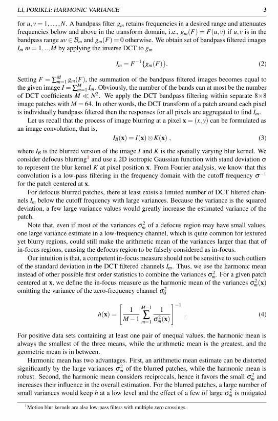
LI, PORIKLI: HARMONIC VARIANCE 3

for u,v = 1, . . . ,N. A bandpass filter gm retains frequencies in a desired range and attenuatesfrequencies below and above in the transform domain, i.e., gm(F) = F(u,v) if u,v is in thebandpass range uv∈Bm and gm(F) = 0 otherwise. We obtain set of bandpass filtered imagesIm m = 1, ..,M by applying the inverse DCT to gm

Im = F−1{gm(F)}. (2)

Setting F = ∑Mm=1 gm(F), the summation of the bandpass filtered images becomes equal to

the given image I = ∑Mm=1 Im. Obviously, the number of the bands can at most be the number

of DCT coefficients M � N2. We apply the DCT bandpass filtering within separate 8×8image patches with M = 64. In other words, the DCT transform of a patch around each pixelis individually bandpass filtered then the responses for all pixels are aggregated to find Im.

Let us recall that the process of image blurring at a pixel x = (x,y) can be formulated asan image convolution, that is,

IB(x) = I(x)⊗K(x) , (3)

where IB is the blurred version of the image I and K is the spatially varying blur kernel. Weconsider defocus blurring1 and use a 2D isotropic Gaussian function with stand deviation σ

to represent the blur kernel K at pixel position x. From Fourier analysis, we know that thisconvolution is a low-pass filtering in the frequency domain with the cutoff frequency σ−1

for the patch centered at x.For defocus blurred patches, there at least exists a limited number of DCT filtered chan-

nels Im below the cutoff frequency with large variances. Because the variance is the squareddeviation, a few large variance values would greatly increase the estimated variance of thepatch.

Note that, even if most of the variances σ2m of a defocus region may have small values,

one large variance estimate in a low-frequency channel, which is quite common for texturedyet blurry regions, could still make the arithmetic mean of the variances larger than that ofin-focus regions, causing the defocus region to be falsely considered as in-focus.

Our intuition is that, a competent in-focus measure should not be sensitive to such outliersof the standard deviation in the DCT filtered channels Im. Thus, we use the harmonic meaninstead of other possible first order statistics to combine the variances σ2

m. For a given patchcentered at x, we define the in-focus measure as the harmonic mean of the variances σ2

m(x)omitting the variance of the zero-frequency channel σ2

0

h(x) =

[1

M−1

M−1

∑m=1

1σ2

m(x)

]−1

. (4)

For positive data sets containing at least one pair of unequal values, the harmonic mean isalways the smallest of the three means, while the arithmetic mean is the greatest, and thegeometric mean is in between.

Harmonic mean has two advantages. First, an arithmetic mean estimate can be distortedsignificantly by the large variances σ2

m of the blurred patches, while the harmonic mean isrobust. Second, the harmonic mean considers reciprocals, hence it favors the small σ2

m andincreases their influence in the overall estimation. For the blurred patches, a large number ofsmall variances would keep h at a low level and the effect of a few of large σ2

m is mitigated

1Motion blur kernels are also low-pass filters with multiple zero crossings.

4 LI, PORIKLI: HARMONIC VARIANCE

by the use of harmonic mean. On the other hand, for the in-focus patches, h still gives largerestimates since most DCT channels have large variances.

Instead of the harmonic mean of variances, the median absolute deviation (MAD) can besubstituted. Nevertheless, MAD disregards the contributions of the variances with small val-ues by pulling the estimate towards the higher values especially when multiple large outliersexist.

2.1 Relation to Noise in Natural ImagesIt is intuitive to draw connections between the proposed in-focus measure and noise analysisof natural images reflecting the super-Gaussian marginal statistics in the bandpass filtereddomains.

We assume the local image noise η(x) is characterized as a Gaussian random variablewith zero mean and σ2

η(x) variance2. The noise contaminated image is then Iη(x) = I(x)+η(x). Based on the observation that noise tends to have more energy in the high frequencybands than natural images, estimation of the global noise variance in an image is usuallybased on the difference image between the noisy image and its low-pass filtered response.

The traditional methodology is to use the relationship between noise variance and otherhigher-order statistics of natural images to obviate the low-pass filtering step. In [24], a noisevariance estimation function is learned by training samples and the Laplacian model for themarginal statistics of natural images in bandpass filtered domains.

Another family of methods uses the relationship between noise variance and image kur-tosis in bandpass filtered domains. Kurtosis is a descriptor of the shape of a probabilitydistribution and defined as κ = µ4/(σ

2)2− 3. It can also be viewed as a measure of non-normality. Due to the independence of noise η to I, and the additive property of cumulants,for each bandpass filtered image Im we have

κm(x) = κ̃m(x)

(σ2

m(x)−σ2η(x)

σ2m(x)

)2

, (5)

where κ̃m(x) and κm(x) represent the kurtosis value of the latent and the noisy Im at x forchannel m.

For natural images, kurtosis has the concentration property in the bandpass filtered do-mains, thus, the kurtosis of an image across the bandpass filtered channels can be approxi-mated by a constant κ(x)≈ κ̃m(x) [21, 31]. In other words, we can estimate the optimal localnoise variance σ2

η(x) and the kurtosis κ by designing a simple least squares minimizationproblem as

minσ2

η ,κ∑m

[√κm(x)−

√κ(x)

(σ2

m(x)−σ2η(x)

σ2m(x)

)]2

, (6)

According to [21], a closed form solution exists

σ2η(x) = α(x) ·h(x) , (7)

where

α(x) =

√κ(x)− 1

M−1 ∑m√

κm(x)√κ(x)

. (8)

2We omit shot noise and other types of noise here. Shot noise follows a Poisson distribution, which can beapproximated by a Gaussian distribution for adequately illuminated images.

LI, PORIKLI: HARMONIC VARIANCE 5

Figure 1: Three regions, defocused (black, red) and focused (blue) from a low DoF image. Thecorresponding kurtosis and variance distributions of blue and red regions in their power spectrum using2D DCT (vectorized, horizontal axis from low-to-high frequencies).

Eqs.(7) and (8) indicate that the noise variance σ2η is related to the in-focus measure h by the

factor α .As we show next, the noise variance estimation algorithms in [21, 31] are limited and do

not apply to low DoF images.Let us take a closer look at α in Eq.(8). Suppose we are given two different patches from

a single image, one extracted from the in-focus region at x1 and the other from the defocusedregion at x2. Since they are extracted from the same image, their local noise variance shouldbe the same, i.e., σ2

η(x1) = σ2η(x2)

3. Moreover, α should be close to 0 for both in-focusand defocused patches since the arithmetic mean of κm is a close estimate of κ regardless ofpatch locations, that is, α(x1) ≈ α(x2) ≈ 0. Since x1 is from the in-focus region, it is verystraightforward that h(x1)� h(x2). Therefore, by Eq.(7), we have σ2

η(x1)� σ2η(x2), which

is inconsistent with our previous assumption. This explains that why the kurtosis estimationin [21, 31] fails for low DoF images and their quadratic formulation shifts high frequency ofthe latent image into noise variance estimations.

This discrepancy can be seen in Fig. 1. As shown, we can easily compute the α and h forboth in-focus region x1 (blue rectangle) and defocused region x2 (red rectangle), and we haveα(x1) = 0.075, h(x1) = 97.12, and α(x2) = 0.016, h(x2) = 0.17, which is consistent withour discussion before. And by Eq.(7) we have σ2

η(x1) = 7.316 and σ2η(x2) = 0.003, contrary

to the assumption of the kurtosis-based noise estimation algorithm. To see our harmonicvariance as a powerful in-focus metric, we mark another defocused region (black) that con-tains slightly more high frequency information than x2. Then we compute the ratio betweenthe in-focus patch x1 and this region for our harmonic variance: 97.12/0.121 = 802, andthe arithmetic mean of the DCT channel variances: 1297.4/84.375 = 15, which intuitive-ly shows that our harmonic variance can competently differentiate the defocus backgroundfrom the in-focus foreground (For clarity, we also show the kurtosis and the variance distri-butions for the blue and red regions in Fig.1).

3 In-Focus Region Segmentation

Contrary to the conventional seeded segmentation algorithms, e.g. graph-cuts [2, 3] and ran-dom walks [6], we use the estimated harmonic variance map h(x) to automatically partitionthe in-focus regions without any user interaction. For more details please refer to [12].

3The assumption is that the input low DoF image is captured under good lighting condition, thus the image ismainly of amplifier noise with Gaussian distribution.

6 LI, PORIKLI: HARMONIC VARIANCE

Algorithm 1: Segmentation Using Laplacian SpectrumInput: Laplacian matrix L of I, harmonic mean h, penalty term β

Output: segmentation fW = I, t = 1 ;while t < itermax & ‖W ( f −h)‖2 < e do

f t = (βL>L+W )−1Wh ;update W according to Eq.(11) ;t = t +1

return the optimal f

To incorporate the harmonic variance values, we compute a graph Laplacian matrix Lfrom the given image I and use it as a constraint. The graph Laplacian spectrum constraintL f = 0 enforces a given image structure on the prior information (in the data fidelity ter-m ‖ f − h‖2). With this constraint, the optimal f should lie in the null-space of L, that is,f should be constant within each connected component of the corresponding graph G. Inmost cases, the binary segmentation results consist of several disconnected components andsegments. Since the estimated f can be represented by a linear combination of the 0 eigen-vectors (the ‘ideal’ basis) of L we are still able to differentiate the foreground componentsfrom the background. In this way, we avoid computing L’s nullity k and its basis, while stillcan use the image structure to regularize the data fidelity term.

The Laplacian matrix L can be used to regularize an optimization formulation by layingit on the structure inherent in I. This enables us to define the in-focus segmentation as aleast-squares constrained optimization problem as

minf‖ f −h‖2, s.t. L f = 0. (9)

From comparative analysis of the harmonic variance maps h and the optimal segmentationf , it is clear that the residual δ (x) = | f −h| has many spatially continuous outliers. The leastsquares fidelity team, however, applies quadratic cost function with equal weighting thatseverely distorts the final estimate in case of outliers. One robust option is to weight largeoutliers less and use the structure information from the Laplacian spectrum constraint torecover the segmentation f . Therefore, we borrow existing principles from robust statistics[7] and adapt a robust functional to replace the least squares term as

minf

ρ( f −h)+β‖L f‖2 , (10)

where ρ is the robust function. We use the Huber function

ρ(x) ={

1 if δ (x)< ε

ε/δ (x) if δ (x)≥ ε(11)

for the reason that it is a parabola in the vicinity of 0 and increases linearly when δ islarge. Thus, the effects of large outliers can be eliminated significantly. When written inmatrix form, we use a diagonal weighting matrix W to represent the Huber weight function.Therefore, the data fidelity term can be simplified as ‖W ( f −h)‖2. As a result, the problemEq.(10) can be solved efficiently in an iterative least square approach. At each iteration, theoptimal f is updated as

f = (βL>L+W )−1Wh . (12)

Our algorithm is shown in Alg. 1.

LI, PORIKLI: HARMONIC VARIANCE 7

input I harmonic variance segmentation GC optimal f segmentation L f = 0

Figure 2: In-focus segmentation results using the proposed harmonic variance measure h.

4 ResultsTo test the performance of the proposed in-focus measure, we conducted experiments onbenchmark images. Fig. 2 shows a typical low DoF scene captured with a large aperturelens. The input image I has gradually changing defocus blurs and the background (fences,farm houses, and etc.) contains strong edges. Our estimated harmonic variance measure ac-curately identifies the in-focus regions (sheep and near grass), and generate nearly consistentvalues for the foreground. When using our harmonic variance to initialize the data cost termof the graph-cut algorithm, it can well model the probability for each pixel belonged to theforeground. However, since our harmonic variance is a patch-based approach, it inevitablygives strong response across the in-focus boundaries, which can cause some artifacts for thegraph-cuts algorithm, as shown in the center of Fig. 2. While the Laplacian based segmenta-tion algorithm can robustly remove the effects of these outliers near the in-focus boundariesand generate an accurate segmentation for this challenging input.

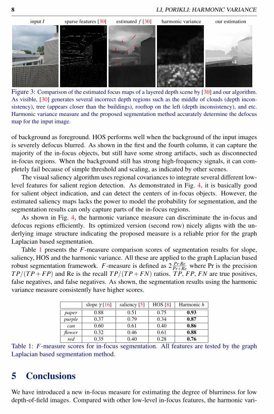
We also compare our method with [30] as shown in Fig. 3. We use a traditional graphLaplacian based segmentation method using `2 norm for a fair comparison instead of thedescribed robust approach in Eq.10. Our measure does not require an edge map (or weightmatrix) yet generates a more accurate defocus map.

Next, we compare our harmonic variance measure with the high-order statistics (HOS) [8],the local power spectrum slope [16, 23], and a state-of-the-art visual saliency estimation al-gorithm [5] for low depth-of-field image feature extraction and in-focus object segmentation.We test the performance of these feature extraction algorithms using the same segmentationalgorithm described in the previous section. In Fig. 4, we show five different natural/man-made scenes with varying defocus conditions and the corresponding defocus maps and seg-mentation results for HOS, saliency, slope and the harmonic variance measure.

In our analysis, we compute the local power spectrum slope γ(x) for a patch size 17×17around each pixel. The local power spectrum slope basically can detect all the in-focusregions, however, it also gives strong responses to complex background, which leads thesegmentation algorithm to mislabel some parts of the background as the foreground.

Instead of computing the image statistics in the frequency domain, HOS works on theimage spatial domain:

HOS(x) = min(C,µ4(x)/D) ,

where µ4(x) is the 4-th order central moment at pixel x computed with local support, and Cand D are empirical parameters for thresholding and scaling. The major drawback of thesestatistic measurements is that they still give strong response if the background features arenot severely defocus blurred, which misleads the segmentation algorithm to label portions

8 LI, PORIKLI: HARMONIC VARIANCE

input I sparse features [30] estimated f [30] harmonic variance our estimation

Figure 3: Comparison of the estimated focus maps of a layered depth scene by [30] and our algorithm.As visible, [30] generates several incorrect depth regions such as the middle of clouds (depth incon-sistency), tree (appears closer than the buildings), rooftop on the left (depth inconsistency), and etc.Harmonic variance measure and the proposed segmentation method accurately determine the defocusmap for the input image.

of background as foreground. HOS performs well when the background of the input imagesis severely defocus blurred. As shown in the first and the fourth column, it can capture themajority of the in-focus objects, but still have some strong artifacts, such as disconnectedin-focus regions. When the background still has strong high-frequency signals, it can com-pletely fail because of simple threshold and scaling, as indicated by other scenes.

The visual saliency algorithm uses regional covariances to integrate several different low-level features for salient region detection. As demonstrated in Fig. 4, it is basically goodfor salient object indication, and can detect the centers of in-focus objects. However, theestimated saliency maps lacks the power to model the probability for segmentation, and thesegmentation results can only capture parts of the in-focus regions.

As shown in Fig. 4, the harmonic variance measure can discriminate the in-focus anddefocus regions efficiently. Its optimized version (second row) nicely aligns with the un-derlying image structure indicating the proposed measure is a reliable prior for the graphLaplacian based segmentation.

Table 1 presents the F-measure comparison scores of segmentation results for slope,saliency, HOS and the harmonic variance. All these are applied to the graph Laplacian basedrobust segmentation framework. F-measure is defined as 2 Pr·Re

Pr+Re where Pr is the precisionT P/(T P+FP) and Re is the recall T P/(T P+FN) ratios. T P, FP, FN are true positives,false negatives, and false negatives. As shown, the segmentation results using the harmonicvariance measure consistently have higher scores.

slope γ [16] saliency [5] HOS [8] Harmonic hpaper 0.88 0.51 0.75 0.93purple 0.37 0.79 0.34 0.87

can 0.60 0.61 0.40 0.86flower 0.32 0.46 0.61 0.88

red 0.35 0.40 0.28 0.76Table 1: F-measure scores for in-focus segmentation. All features are tested by the graphLaplacian based segmentation method.

5 ConclusionsWe have introduced a new in-focus measure for estimating the degree of blurriness for lowdepth-of-field images. Compared with other low-level in-focus features, the harmonic vari-

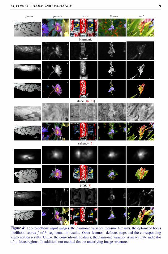
LI, PORIKLI: HARMONIC VARIANCE 9

paper purple can flower red

Harmonic

slope [16, 23]

saliency [5]

HOS [8]

Figure 4: Top-to-bottom: input images, the harmonic variance measure h results, the optimized focuslikelihood scores f of h, segmentation results. Other features: defocus maps and the correspondingsegmentation results. Unlike the conventional features, the harmonic variance is an accurate indicatorof in-focus regions. In addition, our method fits the underlying image structure.

10 LI, PORIKLI: HARMONIC VARIANCE

ance can robustly differentiate the in-focus regions from the defocused background evenwhen the background has strong high frequency responses. We also presented a segmenta-tion algorithm derived from robust statistics and Laplacian spectrum analysis to accuratelypartition out the in-focus regions. In the future, we plan to extend our work for defocusmatting and depth estimation.

References[1] S. Bae and F. Durand. Defocus magnification. Eurographics, 2007.

[2] Y. Boykov and G. Funka-Lea. Graph cuts and efficient ND image segmentation. InternationalJournal on Computer Vision, 70(2):109–131, 2006.

[3] Y. Boykov, O. Veksler, and R. Zabih. Fast approximate energy minimization via graph cuts. IEEETrans. PAMI, 23(11):1222–1239, 2001.

[4] J. Elder and S. Zucker. Local scale control for edge detection and blur estimation. IEEE Trans.PAMI, 20(7):699–716, 1998.

[5] E. Erdem and A. Erdem. Visual saliency estimation by nonlinearly integrating features usingregion covariances. Journal of Vision, 13(4):1–20, 2013.

[6] L. Grady. Random walks for image segmentation. IEEE Trans. PAMI, 28(11):1768–1783, 2006.

[7] P. Huber. Robust statistics. 1981. Wiley, New York.

[8] C. Kim. Segmenting a low-depth-of-field image using morphological filters and region merging.IEEE Trans. on Image Processing, 14(10):1503–1511, 2005.

[9] L. Kovacs and S. Sziranyi. Focus area extraction by blind deconvolution for defining regions ofinterest. IEEE Trans. PAMI, 29(6):1080–1085, 2002.

[10] E. Krotkov. Focusing. International Journal on Computer Vision, 1:223–237, 1987.

[11] A. Levin, B. Fergus, F. Durand, and B. Freeman. Image and depth from a conventional camerawith a coded aperture. ACM Trans. on Graphics, 26(3):70, 2007.

[12] F. Li and F. Porikli. Laplacian spectrum: A unifying approach for enforcing point-wise priors onbinary segmentation. Submitted to ICCV, 2013.

[13] F. Li, J. Sun, J. Wang, and J. Yu. Dual-focus stereo imaging. Journal of Electronic Imaging, 19(4), 2010.

[14] H. Li and K. Ngan. Unsupervised video segmentation with low depth of field. IEEE Trans.Circuits Syst. Video Technol., 17(12):1742–1751, 2007.

[15] H. Lin and X. Chou. Defocus blur parameters identification by histogram matching. J. Opt. Soc.Am. A, 29(8):1694–1706, 2012.

[16] R. Liu, Z. Li, and J. Jia. Image partial blur detection and classification. CVPR, 2008.

[17] T. Liu, J. Sun, N. Zheng, X. Tang, and H. Shum. Learning to detect a salient object. CVPR, 2007.

[18] Z. Liu, W. Li, L. Shen, Z. Han, and Z. Zhang. Automatic segmentation of focused objects fromimages with low depth of field. Pattern Recognition Letters, 31(7):572–581, 2010.

LI, PORIKLI: HARMONIC VARIANCE 11

[19] F. Moreno-Noguer, P. Belhumeur, and S. Nayar. Active refocusing of images and videos. ACMTrans. on Graphics, 26(3):67–75, 2007.

[20] V. Namboodiri and S. Chaudhuri. Recovery of relative depth from a single observation using anuncalibrated camera. CVPR, 2008.

[21] X. Pan, X. Zhang, and S. Lyu. Exposing image splicing with inconsistent local noise variances.ICCP, 2012.

[22] A. Saxena, S.H. Chung, and A.Y. Ng. Learning depth from single monocular images. NIPS,2005.

[23] A. Schaaf and J. Hateren. Modelling the power spectra of natural images: statistics and informa-tion. Vision Research, 36(17):2759–2770, 1996.

[24] A. Stefano, P. White, and W. Collis. Training methods for image noise level estimation on waveletcomponents. EURASIP Journal on Applied Signal Processing, 16:2400–2407, 2004.

[25] C. Swain and T. Chen. Defocus based image segmentation. ICASSP, 1995.

[26] Y. Tai and M. Brown. Single image defocus map estimation using local contrast prior. ICIP,2009.

[27] D. Tsai and H. Wang. Segmenting focused objects in complex visual images. Pattern RecognitionLetters, 19(10):929–949, 1998.

[28] J. Wang, J. Li, and R. Gray. Unsupervised multiresolution segmentation for images with lowdepth of field. IEEE Trans. PAMI, 23(1):85–90, 2001.

[29] C. Won, K. Pyun, and R. Gray. Automatic object segmentation in images with low depth of field.ICIP, 2002.

[30] S. Zhou and T. Sim. Defocus map estimation from a single image. Pattern Recognition, 44(9):1852–1858, 2011.

[31] D. Zoran and Y. Weiss. Scale invariance and noise in natural images. ICCV, 2009.