Harmonic Analysis of Music Using Combinatory Categorial...
183
Harmonic Analysis of Music Using Combinatory Categorial Grammar Mark Granroth-Wilding T H E U N I V E R S I T Y O F E D I N B U R G H Doctor of Philosophy Institute for Language, Cognition and Computation School of Informatics University of Edinburgh 2013
Transcript of Harmonic Analysis of Music Using Combinatory Categorial...
Harmonic Analysis of Music Using
Combinatory Categorial Grammar
Mark Granroth-WildingT
HE
U N I V E RS
IT
Y
OF
ED I N B U
RG
H
Doctor of Philosophy
Institute for Language, Cognition and Computation
School of Informatics
University of Edinburgh
2013


Abstract
Various patterns of the organization of Western tonal music exhibit hierarchical struc-
ture, among them the harmonic progressions underlying melodies and the metre under-
lying rhythmic patterns. Recognizing these structures is an important part of uncon-
scious human cognitive processing of music. Since the prosody and syntax of natural
languages are commonly analysed with similar hierarchical structures, it is reasonable
to expect that the techniques used to identify these structures automatically in natural
language might also be applied to the automatic interpretation of music.
In natural language processing (NLP), analysing the syntactic structure of a sen-
tence is prerequisite to semantic interpretation. The analysis is made difficult by the
high degree of ambiguity in even moderately long sentences. In music, a similar sort of
structural analysis, with a similar degree of ambiguity, is fundamental to tasks such as
key identification and score transcription. These and other tasks depend on harmonic
and rhythmic analyses. There is a long history of applying linguistic analysis tech-
niques to musical analysis. In recent years, statistical modelling, in particular in the
form of probabilistic models, has become ubiquitous in NLP for large-scale practical
analysis of language. The focus of the present work is the application of statistical
parsing to automatic harmonic analysis of music.
This thesis demonstrates that statistical parsing techniques, adapted from NLP with
little modification, can be successfully applied to recovering the harmonic structure
underlying music. It shows first how a type of formal grammar based on one used
for linguistic syntactic processing, Combinatory Categorial Grammar (CCG), can be
used to analyse the hierarchical structure of chord sequences. I introduce a formal
language similar to first-order predicate logical to express the hierarchical tonal har-
monic relationships between chords. The syntactic grammar formalism then serves as
a mechanism to map an unstructured chord sequence onto its structured analysis.
In NLP, the high degree of ambiguity of the analysis means that a parser must
consider a huge number of possible structures. Chart parsing provides an efficient
mechanism to explore them. Statistical models allow the parser to use information
about structures seen before in a training corpus to eliminate improbable interpreta-
tions early on in the process and to rank the final analyses by plausibility. To apply the
same techniques to harmonic analysis of chord sequences, a corpus of tonal jazz chord
sequences annotated by hand with harmonic analyses is constructed. Two statistical
parsing techniques are adapted to the present task and evaluated on their success at
iii

recovering the annotated structures. The experiments show that parsing using a sta-
tistical model of syntactic derivations is more successful than a Markovian baseline
model at recovering harmonic structure. In addition, the practical technique of statis-
tical supertagging serves to speed up parsing without any loss in accuracy.
This approach to recovering harmonic structure can be extended to the analysis of
performance data symbolically represented as notes. Experiments using some simple
proof-of-concept extensions of the above parsing models demonstrate one probabilistic
approach to this. The results reported provide a baseline for future work on the task of
harmonic analysis of performances.
iv

Acknowledgements
The supervision of Mark Steedman has been immensely valuable to me, not only in
bringing the present thesis to fruition, but also for all that I have learned from it regard-
ing academic research, both in the field and more generally. It has, furthermore, been a
great pleasure to work with Mark over the past few years and I shall be sad to lose the
benefit of his vast experience and his deep understanding of computational linguistics
and cognitive science in general. I am also grateful to Sharon Goldwater for valuable
input at various stages of the project and for comments on this thesis.
I have gained a huge amount from meetings and frequent in-depth discussions with
the other members of the research group. Many thanks to Emily Thomforde, Tom
Kwiatkowski, Kira Mourao, Prachya Boonkwan, Michael Auli, Luke Zettlemoyer,
Christos Christodoulopoulos, Aciel Eshky, Greg Coppola, Mike Lewis, Alexandra
Birch, Tejaswini Deoskar, Nathaniel Smith and Bharat Ambati for discussions and ad-
vice. Special thanks must go to Christos, firstly, for all the extensive daily exchanges
over coffee, which have had a substantial impact on my research; and, secondly, for
reading this thesis and providing valuable and detailed comments at a time when he
really should have been concentrating on his own. The parts of this thesis relating to
chord dependencies and dependency evaluation owe much to ideas and insights coming
out of conversations with Joakim Nivre.
My research has benefitted greatly from presenting the work at the following con-
ferences and workshops: Neuromusic IV, SICSA 2011, MML 2012, ICMC 2012. I am
grateful to all concerned for the useful feedback on my work that I received on these
occasions and for the interesting connections that they permitted me to make between
my own work and others’.
I owe a great deal to many of my friends and family members. Two family mem-
bers in particular deserve a special mention. I am immensely grateful to Leonie Wild-
ing for truly remarkable proofreading of this thesis: clear, accurate and amazingly
thorough, not to mention speedy. Hanna Granroth-Wilding has provided invaluable
support through the duration of my PhD and, in particular, during the most stressful
times in the process of writing this thesis. As well as giving me the benefit of the
viewpoint of a quite different scientific discipline, she has helped me to keep things in
perspective and work steadily on, particularly during the final stages of writing.
I gratefully acknowledge the funding I have received to carry out this work from
the Engineering and Social Research Council and FP7 grant 249520 (GRAMPLUS).
v

Declaration
I declare that this thesis was composed by myself, that the work contained herein is
my own except where explicitly stated otherwise in the text, and that this work has not
been submitted for any other degree or professional qualification except as specified.
(Mark Granroth-Wilding)
vi

Table of Contents
1 Introduction 1
2 Structure in Language and Music 52.1 Introduction . . . . . . . . . . . . . . . . . . . . . . . . . . . . . . . 5
2.2 Literature Review: Formal Grammars in the Analysis of Music . . . . 6
2.2.1 Formalizing Music Theory . . . . . . . . . . . . . . . . . . . 7
2.2.2 Syntax and Semantics . . . . . . . . . . . . . . . . . . . . . 8
2.2.3 Musical Grammars . . . . . . . . . . . . . . . . . . . . . . . 11
2.2.4 Probabilistic Music and NLP . . . . . . . . . . . . . . . . . . 20
2.3 Syntax in Language . . . . . . . . . . . . . . . . . . . . . . . . . . . 23
2.4 Combinatory Categorial Grammar . . . . . . . . . . . . . . . . . . . 24
2.5 Functional Structure in Harmony . . . . . . . . . . . . . . . . . . . . 27
2.5.1 The Cadence and Harmonic Function . . . . . . . . . . . . . 28
2.5.2 Coordination . . . . . . . . . . . . . . . . . . . . . . . . . . 30
2.5.3 Jazz Harmony . . . . . . . . . . . . . . . . . . . . . . . . . . 30
2.6 Tonality . . . . . . . . . . . . . . . . . . . . . . . . . . . . . . . . . 31
2.6.1 Consonance and Harmony . . . . . . . . . . . . . . . . . . . 31
2.6.2 Just Intonation . . . . . . . . . . . . . . . . . . . . . . . . . 33
2.6.3 Equal Temperament . . . . . . . . . . . . . . . . . . . . . . 35
2.6.4 Harmonic Interpretation . . . . . . . . . . . . . . . . . . . . 36
2.6.5 Example Interpretations . . . . . . . . . . . . . . . . . . . . 39
2.7 Conclusion . . . . . . . . . . . . . . . . . . . . . . . . . . . . . . . 44
3 A Grammar for Tonal Harmony 453.1 Introduction . . . . . . . . . . . . . . . . . . . . . . . . . . . . . . . 45
3.2 Tonal Harmonic Interpretation Semantics . . . . . . . . . . . . . . . 46
vii

3.2.1 The Lambda Calculus as Notation . . . . . . . . . . . . . . . 47
3.2.2 Interpretation of Tonics . . . . . . . . . . . . . . . . . . . . . 48
3.2.3 Interpretation of Cadences . . . . . . . . . . . . . . . . . . . 50
3.2.4 Coordination of Cadences . . . . . . . . . . . . . . . . . . . 51
3.2.5 Multiple Cadences: Development . . . . . . . . . . . . . . . 53
3.2.6 Colouration: Empty Semantics . . . . . . . . . . . . . . . . . 54
3.2.7 Extracting the Tonal Space Path . . . . . . . . . . . . . . . . 55
3.2.8 Representation as Dependency Graphs . . . . . . . . . . . . . 58
3.3 CCG for Harmonic Syntax . . . . . . . . . . . . . . . . . . . . . . . 59
3.4 A Grammar for Jazz . . . . . . . . . . . . . . . . . . . . . . . . . . . 63
3.4.1 The Rules . . . . . . . . . . . . . . . . . . . . . . . . . . . . 63
3.4.2 The Lexicon . . . . . . . . . . . . . . . . . . . . . . . . . . 65
3.5 Key Structure . . . . . . . . . . . . . . . . . . . . . . . . . . . . . . 70
4 Building an Annotated Corpus 734.1 Introduction . . . . . . . . . . . . . . . . . . . . . . . . . . . . . . . 73
4.2 Chord Sequence Data . . . . . . . . . . . . . . . . . . . . . . . . . . 74
4.2.1 Data Format . . . . . . . . . . . . . . . . . . . . . . . . . . 74
4.2.2 Cross-Validation . . . . . . . . . . . . . . . . . . . . . . . . 76
4.3 Annotating a Unique Gold-Standard Interpretation . . . . . . . . . . 77
4.4 Annotation Procedure . . . . . . . . . . . . . . . . . . . . . . . . . . 82
4.4.1 Analysis Decisions . . . . . . . . . . . . . . . . . . . . . . . 85
4.5 Omissions . . . . . . . . . . . . . . . . . . . . . . . . . . . . . . . . 87
4.5.1 Consistency . . . . . . . . . . . . . . . . . . . . . . . . . . . 88
4.6 Lexical Ambiguity . . . . . . . . . . . . . . . . . . . . . . . . . . . 90
4.7 Conclusion . . . . . . . . . . . . . . . . . . . . . . . . . . . . . . . 91
5 Statistical Parsing of Chord Sequences 935.1 Introduction . . . . . . . . . . . . . . . . . . . . . . . . . . . . . . . 93
5.2 Supertagging Experiments . . . . . . . . . . . . . . . . . . . . . . . 95
5.2.1 Supertagging . . . . . . . . . . . . . . . . . . . . . . . . . . 95
5.2.2 N-Gram Supertagging Models . . . . . . . . . . . . . . . . . 97
5.2.3 Using the C&C Supertagger . . . . . . . . . . . . . . . . . . 102
5.2.4 Evaluation . . . . . . . . . . . . . . . . . . . . . . . . . . . 103
5.2.5 Results . . . . . . . . . . . . . . . . . . . . . . . . . . . . . 104
5.3 Statistical Parsing Experiments . . . . . . . . . . . . . . . . . . . . . 107
viii
5.3.1 Introduction . . . . . . . . . . . . . . . . . . . . . . . . . . . 107
5.3.2 CKY Parsing . . . . . . . . . . . . . . . . . . . . . . . . . . 107
5.3.3 Hockenmaier’s Parsing Model for CCG . . . . . . . . . . . . 109
5.3.4 PCCG for Parsing with the Jazz Grammar . . . . . . . . . . . 112
5.3.5 Tonal Space Path HMM Baseline . . . . . . . . . . . . . . . 116
5.3.6 Aggressive Backoff . . . . . . . . . . . . . . . . . . . . . . . 119
5.3.7 Evaluation . . . . . . . . . . . . . . . . . . . . . . . . . . . 121
5.3.8 Results . . . . . . . . . . . . . . . . . . . . . . . . . . . . . 124
5.4 Discussion and Conclusion . . . . . . . . . . . . . . . . . . . . . . . 126
6 Parsing Note-Level Performance Data 1296.1 Introduction . . . . . . . . . . . . . . . . . . . . . . . . . . . . . . . 129
6.2 Data Representation: MIDI . . . . . . . . . . . . . . . . . . . . . . . 131
6.3 Adding MIDI to the Jazz Corpus . . . . . . . . . . . . . . . . . . . . 131
6.4 Pipeline Approach . . . . . . . . . . . . . . . . . . . . . . . . . . . 132
6.4.1 Chord Recognizer as a Frontend to the Supertagger . . . . . . 132
6.4.2 Supertagging a Chord Lattice . . . . . . . . . . . . . . . . . 135
6.4.3 HMM Baseline . . . . . . . . . . . . . . . . . . . . . . . . . 139
6.4.4 Evaluation . . . . . . . . . . . . . . . . . . . . . . . . . . . 140
6.4.5 Results . . . . . . . . . . . . . . . . . . . . . . . . . . . . . 147
6.4.6 Discussion . . . . . . . . . . . . . . . . . . . . . . . . . . . 148
6.5 Future Work . . . . . . . . . . . . . . . . . . . . . . . . . . . . . . . 149
6.6 Conclusion . . . . . . . . . . . . . . . . . . . . . . . . . . . . . . . 152
7 Conclusion 155
Bibliography 159
ix

Table of Examples
2.1 Linguistic CCG function application . . . . . . . . . . . . . . . . . . . 25
2.2 Linguistic CCG derivation with semantics . . . . . . . . . . . . . . . . 26
2.3 Linguistic composition rule . . . . . . . . . . . . . . . . . . . . . . . . 26
2.4 Linguistic coordination rule . . . . . . . . . . . . . . . . . . . . . . . . 27
2.5 Tonal space analysis of the Basin Street Blues . . . . . . . . . . . . . . 39
2.6 Tonal space analysis of the opening of BWV 553 . . . . . . . . . . . . 41
2.7 Tonal space analysis of Autumn Leaves . . . . . . . . . . . . . . . . . . 42
3.1 Function application with the lambda calculus . . . . . . . . . . . . . . 47
3.2 Function application for the semantics of a passive verb . . . . . . . . . 48
3.3 Logical forms for the interpretation of tonics . . . . . . . . . . . . . . . 50
3.4 Derivation of a harmonic interpretation from its constituents . . . . . . 51
3.5 Derivation of a harmonic interpretation using composition . . . . . . . 51
3.6 Conjunction of cadence logical forms by coordination . . . . . . . . . . 52
3.7 Coordinated cadence logical form applied to its resolution . . . . . . . . 52
3.8 Coordinating more than two cadences . . . . . . . . . . . . . . . . . . 53
3.9 Resolution of a dominant onto a coordination . . . . . . . . . . . . . . 53
3.10 Concatenation of two resolved cadences by the development rule . . . . 54
3.11 Concatenation of a tonic with a resolved cadence . . . . . . . . . . . . 54
3.12 Colouration chord with empty semantics . . . . . . . . . . . . . . . . . 54
3.13 Derivation of a cadence logical form constrained by syntactic types . . . 61
3.14 Syntactic derivation of a cadence by composition . . . . . . . . . . . . 62
3.15 Syntactic derivation of a coordinated cadence . . . . . . . . . . . . . . 62
3.16 Syntactic types for a cadence from Can’t Help Lovin’ Dat Man . . . . . 63
3.17 Repeated tonic chords, including a substitution, interpreted by a category
produced by the tonic repetition rule . . . . . . . . . . . . . . . . . . . 65
xi

3.18 Extended cadence derivation with semantics . . . . . . . . . . . . . . . 69
3.19 Derivation of cadence from Can’t Help Lovin’ Dat Man . . . . . . . . . 69
3.20 Rough sketch of a syntactic derivation permitting interpretation of hier-
archical modulation . . . . . . . . . . . . . . . . . . . . . . . . . . . . 72
4.1 The order of composition and coordination in a derivation does not affect
the result . . . . . . . . . . . . . . . . . . . . . . . . . . . . . . . . . . 78
4.2 Categories assigned to a cadence from Alfie . . . . . . . . . . . . . . . 82
4.3 Categories assigned to a cadence from Alfie, with schema names . . . . 85
5.1 Chord sequence for a cadence from Can’t Help Lovin’ Dat Man (repeated) 93
5.2 Derivation of an implausible interpretation of Can’t Help Lovin’ Dat
Man cadence . . . . . . . . . . . . . . . . . . . . . . . . . . . . . . . 94
xii

Table of Acronyms
AA anotation accuracy 89
AST adaptive supertagging (Clark & Curran, 2004a) 97, 103, 125, 127, 135, 137,
157
CCG Combinatory Categorial Grammar (Steedman, 2000) iii, 2, 5, 9, 15, 20, 24–26,
44–46, 59, 63, 65, 71, 77, 90, 95, 96, 102, 107–109, 113, 114, 155–157
CKY Cocke-Kasami-Younger (Harrison, 1978) 107, 108, 111
DR dependency recovery 88, 89, 123–125, 140, 141, 146, 147, 157
EM expectation-maximization 101, 134
GTTM A Generative Theory of Tonal Music (Lerdahl & Jackendoff, 1983; Jackend-
off, 1991; Lerdahl, 2001) 11–18
HMM hidden Markov model (Rabiner & Juang, 1986) 20, 98–101, 104, 114–118,
127, 133–135, 139, 148–150
MIDI Musical Instrument Digital Interface (MIDI Manufacturers Association, 1996)
131–134, 136–142, 146–153, 157
MIR music information retrieval 21, 130
NLP natural language processing iii, 1–3, 5, 7, 20, 21, 23, 58, 73, 74, 94, 96–98,
100–102, 106, 120, 123, 130, 140, 156, 158
ODR optimized dependency recovery 141, 142, 146–148
xiii

PCCG probabilistic CCG (Hockenmaier, 2001) 109, 110, 112, 125–127
TSED tonal space edit distance 88, 89, 123–125, 140, 148, 157
xiv

CHAPTER 1Introduction
Hierarchical structure can be identified in the organization of Western tonal music, for
example in the rhythmic patterns of the melodies and the harmonic progressions that
underly them. The prosody and syntax of natural languages are commonly analysed
as being organized according to similar hierarchical structures, represented as tree dia-
grams that divide a passage of speech or text recursively into its constituents, down to
the level of individual words. It is, therefore, reasonable to expect that the techniques
used to identify and process these structures automatically in natural language might
profitably be applied to the automatic interpretation of music.
In natural language processing (NLP), analysing the syntactic structure of a sen-
tence is usually a prerequisite to semantic interpretation. The analysis is a non-trivial
task, as a result of the high degree of ambiguity in even moderately long sentences. In
music, a similar sort of structural analysis, over sequences exhibiting a similar degree
of ambiguity, is fundamental to tasks such as key identification and score transcrip-
tion. These and other tasks depend on both a harmonic (tonal) analysis and a rhythmic
(metrical) analysis.
There is a long history of the application of linguistic analysis techniques to musical
analysis (among others, Meyer, 1956; Cooke, 1959; Bernstein, 1976; Smoliar, 1976;
Roads & Wieneke, 1979; Baroni et al., 1983), with varying degrees of formality. Some
of this work has explored various applications of formal grammars to the analysis
1

2 Chapter 1. Introduction
of hierarchical structure (Winograd, 1968; Keiler, 1981; Lerdahl & Jackendoff, 1983;
Steedman, 1996; Rohrmeier & Cross, 2009). Meanwhile, in the field of NLP, statistical
modelling, in particular in the form of probabilistic models, has become ubiquitous for
large-scale practical analysis of language (for example Collins, 1997; Hockenmaier
& Steedman, 2002; Clark & Curran, 2004b; Auli & Lopez, 2011). The focus of the
present thesis is on the application of formal grammars and related statistical models
of language to the task of automatically analysing music. I argue that the structures
that underly the harmonic progressions of Western tonal music have a syntax similar
to that of natural languages and that the unconscious processing of these structures by
listeners can be modelled using a formalism similar to those used to model linguistic
syntactic processing. I address the question that naturally follows of to what extent the
statistical parsing techniques used to perform automatic linguistic analysis in NLP can
be applied to automatic harmonic analysis of music.
This thesis demonstrates that statistical parsing techniques, adapted from NLP with
little modification, can be successfully applied to recovering harmonic structure. It
shows first how a type of formal grammar similar to one used for linguistic syntactic
processing, Combinatory Categorial Grammar (CCG, Steedman, 2000), can be used to
analyse the hierarchical structure of chord sequences. Harmonic structure can be anal-
ysed in terms of relationships between chords expressed in the tonal space of Longuet-
Higgins (1962a,b). Several of the authors cited above have proposed grammars to for-
malize the structure of tonal relationships between chords and the analyses produced
by the grammar presented here bear considerable similarity to these. The proposed
grammar differs from previous work in two main respects. Firstly, it makes the distinc-
tion advocated by Steedman (2000) between semantics – the formal structural analysis
of interest – and syntax – the rules that govern the process of deriving the structure
from an unstructured input. Though the distinction has in general not been made ex-
plicitly, previous work has focused primarily on the former: the structures that underly
harmony as unconsciously understood by a listener. The explicit separation of these
components of the analysis made by CCG permits an account of the process of syntac-
tic derivation in which the structure of a derivation need not strictly follow the structure
that is derived. As a result, a parser is able to perform a more incremental (that is, left-
to-right) analysis and the grammar may use a less constrained notion of constituency.
Secondly, taking advantage of this latter feature of the formalism, the grammar treats
unfinished cadences (or ‘half-cadences’) in a new way. Whilst maintaining an analy-
sis of extended cadences as structures with a right-branching embedding, it permits a

3
left-branching embedding of the constituents built during a derivation, allowing unfin-
ished cadences to be treated as constituents. The interpretation of multiple unfinished
cadences as sharing an eventual resolution is structurally analogous to a type of coordi-
nation common in natural language. Together with a handling of modulation similar to
some of the previous work, the result is a grammar capable of analysing a wide range
of musical structures within a particular genre and easily adaptable to other genres.
The present work introduces a formal language similar to first-order predicate logic to
express tonal relationships. The syntactic grammar formalism then serves as a mech-
anism to map unstructured chord sequences onto their semantics represented in this
language. A grammar using the formalism is presented for analysing chord sequences
of jazz standards, which tend to feature particularly complex patterns of structural
embedding in their harmony. Both the formal language of harmonic analysis and the
grammar formalism are further developments of the previous work of Steedman (1996)
and the author (Wilding, 2008). They are described in full in chapter 3.
In NLP, the high degree of ambiguity of syntactic analysis means that a parser must
consider a huge number of possible structures. Chart parsing provides an efficient
mechanism by which to explore them. The addition of statistical models allows the
parser to use information about the frequency of structures seen before in a training
corpus to eliminate improbable interpretations early on in the process and to rank the
final analyses by plausibility. To apply the same techniques to harmonic analysis,
a corpus of chord sequences annotated with good analyses is required. Chapter 4
documents the construction of such a corpus of analyses using the grammar and some
of the difficulties encountered in the process.
The present work follows in a long tradition of linguistic-style grammatical analy-
ses of music. It is, however, the first to apply statistical models of grammatical structure
to wide-coverage automatic harmonic analysis. Chapter 5 describes the adaptation of
two statistical parsing techniques and their evaluation: a probabilistic model of gram-
matical derivations and a supertagger, allowing fast approximate parsing. The corpus
is small, which puts limitations on the statistical models that can be trained using it.
The experiments in chapter 5 with supertaggers make it clear that the type of history-
based sequence models tested can only use a small amount of contextual information.
Parsing experiments in chapter 5 show that parsing using the model of derivations
is successful at recovering harmonic analyses, improving substantially over a baseline
Markovian model. Using the derivation model together with the supertagger, the parser
achieves a similar improvement over the baseline with much shorter processing time.
4 Chapter 1. Introduction
Chord sequences provide a useful abstraction of musical input to demonstrate the
effectiveness of the parsing techniques and it is an assumption of this analysis tech-
nique that segmentation of the input into passages of similar underlying harmony must
feature in any harmonic analysis of musical data at the level of performed or written
notes. Transcribed chord symbols, of the sort used as input to a parser in the experi-
ments of chapter 5, approximate a segmentation into harmonic units that is required for
a harmonic analysis of the notes of a performance or a score. It should, therefore, be
possible in principle at least to extend the same analysis techniques to the interpreta-
tion of data representing an actual musical performance. Such an extension would have
useful applications in many practical tasks, for example in the field of music informa-
tion retrieval, as well as being of interest to constructing a more convincing account
of human cognition of musical structure. Chapter 6 introduces some extensions of
the parsing techniques to handle musical performance data, symbolically represented
as a stream of notes. The models presented are simple and theoretically rather unsat-
isfactory, but serve to demonstrate one manner in which the models previously used
for chord sequence analysis can be extended to this harder task. The results reported
provide a baseline for future work on the task of harmonic analysis of performance
data.

CHAPTER 2Structure in Language and Music
2.1 Introduction
Many tasks in NLP, such as query understanding and sentiment analysis, are dependent
on analysis of the predicate-argument structure of sentences, performed by parsing.
In this thesis, I argue that the task of natural language parsing is analogous to the
musical task of analysis of the tension-resolution structures found in tonal harmony.
This analogy has previously been exploited for harmonic and other types of musical
analysis. The analogy leads naturally to the question of whether the well-developed
techniques applied to the language parsing task in NLP can equally be applied to a
similar parsing task defined for harmony.
This chapter presents an overview of the important background to the present goal
of adapting parsing techniques to harmonic analysis. Section 2.2 surveys previous
work in this field and discusses the present work’s relation to other grammatical ap-
proaches to musical analysis. Sections 2.3 and 2.4 introduce the concept of syntactic
parsing and the grammatical formalism, CCG, which I later take as the basis for a
grammar of harmony. Section 2.5 describes informally the sorts of structures found
in tonal harmony that this work is concerned with analysing. Section 2.6 outlines a
theory of tonal music which provides a formal model for harmonic analysis of those
structures.
5
6 Chapter 2. Structure in Language and Music
2.2 Literature Review: Formal Grammars in the Analy-
sis of Music
The nature of human response to music, its relationship to the musical signal and the
mechanisms by which a signal is interpreted, internally represented and remembered
by a listener have long been a subject of wide-ranging investigation (Euler, 1739;
Helmholtz, 1862; Meyer, 1956; Cooke, 1959; Desain & Honing, 1992). Music as a
communicative system resembles natural languages in that it requires the unconscious
inference of structures ambiguous in the signal in order to be understood by a listener
(Keiler, 1981). Relating these cognitive structures to the meaning conveyed by the
music is a critical part of understanding the nature of musical communication. Besides
studying the sorts of meaning that music is capable of conveying, it is prerequisite to
such an endeavour to explain the cognitive structures that support communication of
musical meaning – the structures underlying perception of, for example, melody, har-
mony and rhythm – in much the same terms as the corresponding question for language
(Longuet-Higgins, 1978).
A listener hearing a sentence in English must be aware of certain linguistic struc-
tures underlying it in order to derive the speaker’s meaning. Inference of the logical
relationships between the entities, actions and events denoted by the words is an es-
sential part of the semantic interpretation of the sentence. Identifying these relations
requires connections to be made between arbitrarily distant words in the sentence.
Similar close relationships exist between musical elements linearly (that is, chronolog-
ically) distant in the signal processed by a human listener. In both music and language,
the structural organization underlying the signal plays an essential role in interpreting
and memorizing it and, in both cases, this is performed unconsciously by the listener.
This observation is fundamental to much work that has drawn on the links between
music and language (Meyer, 1956; Longuet-Higgins, 1962a,b; Smoliar, 1976; Lerdahl
& Jackendoff, 1983). Cooke (1959, p. 33) takes it as the basis for an attempt to explain
the nature of musical emotional expression. He describes the technical construction of
music as the ‘magnificent craftsmanship whereby composers express their emotions’,
claiming that it is ‘unintelligible to the layman, except emotionally’. In other words, he
recognizes that structural organization must play a part even for an untrained listener
in the emotional effects of music, albeit unconsciously.

2.2. Literature Review: Formal Grammars in the Analysis of Music 7
In this section, I examine some formal approaches to characterizing the struc-
tural processing of music, and in particular harmony, performed by a listener. I relate
them to a particular approach to a related task in NLP – the analysis of the semantic
predicate-argument relations in sentences by syntactic parsing using formal grammars.
2.2.1 Formalizing Music Theory
There is a long history in Western music theory of informal description of musi-
cal structure, most commonly as an aid to composers (for example, Cooke, 1959;
Schenker, 1906). Many authors have advocated the formalization of intuitions regard-
ing musical organization, some drawing on formal tools from linguistics (see below)
and others on other means of formal description, including imperative programming
languages (Smoliar, 1976; Forte, 1967; Longuet-Higgins & Steedman, 1971; Baroni
et al., 1983; Temperley & Sleator, 1999). Baroni et al. (1983) define the fundamen-
tal role of scholarly discussion of music as providing a theoretical framework which
may serve ‘as a formal model for the phenomena it describes and thus be capable of
“explaining” the complexity of music as an instrument of communication and culture.’
Temperley (2007) advocates approaching the theory of music cognition by proposing
computational models on the basis that, whilst the ability of a model to support auto-
matic computation does not prove its suitability as a model of human cognition, it does
satisfy an important requirement of a plausible model.
In his series of six Norton Lectures, Bernstein (1976) proposed the application of
Chomsky’s (1965) formal grammars to the analysis of music. Although the specifics of
Bernstein’s proposal have been widely rejected for a range of reasons, his idea served
as the inspiration for several lines of research exploring the formal and cognitive corre-
spondences between music and language. In a response to Bernstein’s proposal, Keiler
(1978), whilst supporting the exploration of application of formal grammars to musi-
cal analysis, urges caution in drawing correspondences. The approach he proposes is
to look for connections between linguistic and musical analysis only where they are
dictated by characteristics that arise independently in the two domains, emphasizing
the dangers of beginning with assumptions regarding the specific correspondences we
expect to find. Lerdahl & Jackendoff (1983) make a similar point, observing that their
own analysis turns out not to resemble linguistic theories very closely. Katz & Peset-
sky’s (2011) recent approach, on the other hand, is quite different. Although they take
Lerdahl & Jackendoff’s (1983) analysis as their starting point, they attempt to show that

8 Chapter 2. Structure in Language and Music
it can after all be re-expressed in terms very similar to linguistic theories. Contrary to
Keiler’s argument, they begin with the hypothesis that music and language are prod-
ucts of a single cognitive system and that, therefore, theories of musical and linguistic
structure should be maximally aligned. Bernstein’s was one of several early propos-
als for the formal analysis of musical cognition using grammars (Winograd, 1968;
Lindblom & Sundberg, 1969) and subsequently a variety of approaches have been ex-
plored (Longuet-Higgins, 1978; Keiler, 1981; Lerdahl & Jackendoff, 1983; Steedman,
1984; Johnson-Laird, 1991; Steedman, 1996; Pachet, 2000; Chemillier, 2004; de Haas
et al., 2009; Rohrmeier & Cross, 2009), to which much of the remainder of this review
will be devoted. Longuet-Higgins & Lisle (1989) sketch an application of Chomskian
grammars to music in which a language corresponds to a musical idiom, an utterance
to a composition in that idiom and logical meaning to affective meaning. The corre-
spondence is the same that is used by Lerdahl & Jackendoff (1983) (though Longuet-
Higgins & Lisle claim their generative theory of music to be closer to the Chomskian
paradigm).
2.2.2 Syntax and Semantics
Steedman (2002) makes a connection between certain fundamental operations involved
in syntactic processing and operations in the reasoning that underlies planning a series
of actions in order to achieve a goal. The importance of this connection is that it sup-
ports a theory of human linguistic processing which is deeply connected to the more
general human capacity to represent and reason about actions and their consequences,
a connection suggested by neurological literature on language processing and child
language acquisition. If the unconscious structural organization of a linguistic signal
can be explained in terms of a set of operations having their origin in motor planning, it
is likely that a similar explanation can be provided for the organization of structurally
similar musical relationships, such as those formalized by Keiler (1981) or Johnson-
Laird (1991). Furthermore, the possibility that operations from the same evolved ca-
pacity for planning can offer an explanation of cognition of both language and music
provides new grounds for Katz & Pesetsky’s (2011) programme searching for a theory
of musical competence that resembles linguistic theory as closely as possible in the
hope that the result may shed light on the cognitive capacity common to the two1.
1 Honing (2011a,b) even suggests, on the basis of experiments with young babies, that certain typesof cognitive processing of music might be more primitive than language processing, although his exper-iments concern perception of pitch and metre at a level which has little impact on an explanation of our

2.2. Literature Review: Formal Grammars in the Analysis of Music 9
Steedman (2000) argues for a theory of syntax that differs from that underlying
many earlier treatments of linguistic grammar. Rather than being seen as a level of
representation of linguistic structure, it is treated as a characterization of the process
by which a semantic interpretation is derived compositionally from the language’s spo-
ken form. The semantic interpretation includes a logical form, a representation of the
predicate-argument relationships expressed in the surface form. The syntactic com-
ponent of a grammar serves to enforce language-specific constraints on the ordering
and combination of constituents in mapping the linguistic signal to its interpretation.
Under this approach, the meaning representation is quite separate to the syntactic con-
structs available to derive it from sentences. The result is that an account of syntac-
tic processing need not strictly reflect the structure of the meaning representation in
the intermediate structures it builds. For example, the fact that the logical form of
a particular sentence takes the form of a right-branching structure need not prevent
the left-branching syntactic derivation that better explains a hearer’s ability to perform
an incremental analysis. Steedman presents the grammar formalism of CCG, which
expresses a transparent connection between a compositional semantics and the syntac-
tic constituents by which it is induced from the surface form and which permits the
required non-standard derivational structures.
A feature by no means unique to this breed of linguistic theory, but made more
explicit by the transparent pairing of syntax and semantics, is that the purpose of spec-
ifying a grammar for a natural language is not to define a set of sentences permissible
in a language, nor to provide a test for the permissibility of a particular sentence, but to
explain the relationship between the elements of a sentence and the structure of the sen-
tence’s meaning. Lerdahl & Jackendoff (1983) note that a misunderstanding of the role
of a formal grammar in this way has led some to a mistaken understanding, or indeed a
complete rejection, of the applicability of formal grammars to a theory of music. This
separation also provides an answer to Narmour’s rejection of a theory of music based
on Chomsky’s (1965) transformational grammars. Narmour (1977, pp. 116–119) ar-
gues against a transformational grammar approach to music (in particular, against a
grammatical formalization of Schenkerian theory) on the grounds that it is impossi-
ble to separate the structure of the interpretation from the structure that derives it. He
argues about Schenkerism in general that it fails to separate analysis from methodol-
ogy. Steedman’s theory of grammar, however, does just that in its explicit separation
of logical semantics from the rules of syntax constraining its derivational process.
capacity to process complex musical structures.
10 Chapter 2. Structure in Language and Music
Longuet-Higgins (1978) points out that, whilst many authors had previously at-
tempted to define the meaning expressed by music (Hindemith, 1942; Tovey, 1949;
Meyer, 1956; Cooke, 1959) and its relation to musical structure, none had addressed
the issue of providing a theory of the cognitive structures that underly our ability to
interpret, remember and recognize music. That is, they do not explain the structures
that we perceive when we hear a piece of music and how they relate to the sound sig-
nal. This question corresponds to the question in the linguistic domain of what logical
structures are conveyed by a speech signal (for example the logical forms discussed
above) that allow us to interpret it with respect to some notion of the real world and
how the speech signal is processed to retrieve them. In formalizing musical structure
and the syntax that relates it to a musical surface form, it is not particularly impor-
tant that the meaning expressed by music is of a very different kind to that typically
expressed by language. London (2011) rejects a linguistic-style treatment of musical
syntax for several reasons, among them its lack of referential-semantic content. This
criticism is put in a different light by Steedman’s (2000) view of syntax. A logical
form such as eats′(keats′,beets′) for the sentence Keats eats beets cannot serve as an
interpretation of the sentence’s meaning with respect to a model of the world without
some connection between the predicate eats′ and the familiar concept of consuming
food, and so on. Such a connection is assumed to be available in the interpretation
of the sentence as far as the logical form is concerned in the form of a model theory.
Regardless of the meaning associated with eats′, it is essential to understanding the
denotation of the sentence that the listener recognize the particular predicate-argument
structure that the logical form expresses. Likewise, regardless of the affective or in-
dexical meaning that might follow (in the style of Meyer, 1956 or Cooke, 1959), in
order to build the prerequisite cognitive structure to interpret the chord sequence D7
G7 C in the key of C major it is essential to recognize the dominant relation of the G7
with respect to the C and the secondary dominant relation of the D7 to the G7. Despite
the absence of a full account of musical meaning, we do have a fairly good knowledge
of many of the structures essential to perception of music: phrases, metre, polyphony,
harmony, etc. This review focuses on work whose goal is to characterize the cognitive
structures and processes that support the perception of musical meaning. I, therefore,
will not talk here about work on the types of meaning conveyed by music or how they
relate to these structures. (For a thorough review, see Monelle, 1992.)

2.2. Literature Review: Formal Grammars in the Analysis of Music 11
2.2.3 Musical Grammars
In this section, I discuss in more detail several accounts of structure in tonal music that
directly relate to the present thesis. In particular, I consider applications of linguistic-
style grammars in the light of the above view of the role of syntax. In these terms, most
of the works discussed are primarily concerned with a theory of the structures that con-
stitute the semantics of music (in the same sense in which a logical form expresses the
semantics of a sentence) and less with a theory of the computational process required
to derive the structures from a musical surface.
2.2.3.1 Lerdahl and Jackendoff
A Generative Theory of Tonal Music (GTTM, Lerdahl & Jackendoff, 1983; Jackend-
off, 1991; Lerdahl, 2001) has been one of the most influential works on the application
of theories inspired by linguistics to music. GTTM sets out a thorough account of cer-
tain types of structure underlying music. Their analysis begins with two independent
structures: grouping structure, representing the hierarchical segmentation of the music
into phrases, and metrical structure, representing the organization of rhythm to align
with a number of levels of regular patterns formalized as a metrical grid. Both of these
precede and contribute to two further structures: time-span reduction, denoting the rel-
ative structural importance of notes, and prolongation reduction, a structure of tension
and resolution in melody. The structures are derived by a collection of semi-formal
preference rules governing the order in which notes are connected to the structures and
the type of relationship expressed by the connection. Lerdahl & Jackendoff (1983)
state that the theory is concerned not with the cognitive processes of a listener, but
rather with ‘the final state of his understanding’. Jackendoff (1991) describes GTTM
as ‘an account of the abstract structures available to the listener’ and ‘of the principles
available to the listener to assign abstract structure to pieces of music’. Thus GTTM
makes an important contribution to the formalization of the cognitive structures that
underly music, but does not attempt to represent any aspect of the process by which
they are unconsciously produced. Jackendoff (1991) further outlines some principles
for the construction of an interpretative mechanism, a parser, that explain how the lis-
tener can build the structures in real time. These include an approach to ambiguity
now common in statistical parsing of natural language and applied to musical parsing
in the present thesis, though Jackendoff does not propose the use of statistics to model
the relative plausibility of ambiguous interpretations.

12 Chapter 2. Structure in Language and Music
Clarke (1986) claims that Lerdahl & Jackendoff do not take due consideration of
Chomsky’s distinction between competence – an idealized system of linguistic knowl-
edge shared by native speakers – and performance – the practical issues that come
into play in the actual use of a language for communication. From their aim of mod-
elling the final state of understanding of an idealized experienced listener, Lerdahl &
Jackendoff appear, like Chomsky, to position their work firmly in the domain of com-
petence. Clarke (1986) questions this classification, pointing out several psychological
aspects of the theory discussed in GTTM, suggesting that they are after all interested
in the implications for a theory of performance. Nevertheless, a theory of competence
grammar cannot be divorced from issues of performance, since the two must have de-
veloped together as part of a single system (Steedman, 2000, p. 261). This holds for
musical grammar just as for linguistic grammar, since music serves its primary com-
municative purpose through its capacity to be interpreted unconsciously by a listener
in real time. A competence grammar must be able to support a plausible theory of a
performance mechanism, providing, for example, any required notions of constituency
and incrementality. A theory of what is computed, as opposed to one of how the
computation is carried out (to use the terminology of Johnson-Laird, 1991), should,
therefore, not eschew consideration of the computational properties of the processing
that it entails. Rosner (1984) points out the particular danger of dismissing as irrele-
vant this aspect of a theory while making such bold claims as Lerdahl & Jackendoff
do regarding the innateness of musical cognition and consequent universality of some
aspects of their theory.
Jackendoff (1991) sets out four necessary components of a theory of music percep-
tion, accounting for (1) abstract structures available to a listener; (2) the principles by
which a listener may assign these structures to music; (3) how the principles are applied
in real time and (4) the facilities in the mind for applying the principles. He claims that
Lerdahl & Jackendoff (1983) addressed (1) and (2) and sketches an approach to pro-
viding (3) for GTTM. The outlined computational model, a parallel multiple-analysis
parser, is essentially the approach to parsing widely accepted as the basis for statistic
parsers in the natural language parsing community, though Jackendoff does not link the
notion of plausibility to anything as concrete as a statistical model. Simply augmenting
the rules of GTTM with a system of priorities, as originally suggested by Lerdahl &
Jackendoff (1983) and implemented by Hamanaka et al. (2006) might appear to take
a step towards answering the criticism of, among others, Longuet-Higgins (1983) that
GTTM fails to constitute a formal analysis. However, Clarke (1986) notes that Ler-

2.2. Literature Review: Formal Grammars in the Analysis of Music 13
dahl & Jackendoff are mistaken in viewing the indeterminacy of GTTM as a reflection
of the inconsistency of human analysis: instead, the model should provide definite
analyses, with specific points of divergence between alternative, but nonetheless well-
defined, analyses. The theory should explain in precise terms how a human listener
can construct an unambiguous analysis of some passages of music. Where ambiguity
arises in human interpretation, it should be accounted for as a choice between multiple
alternative interpretations, each deemed acceptable by the theory. Jackendoff (1991)
takes quite a different view of ambiguity to Hamanaka et al. (2006), closer to Clarke’s
(1986). His proposed parser would in principle be capable of outputting multiple fully
formed analyses.
The similarities between GTTM and Schenkerian analysis (Schenker, 1906) are
seen by the authors as a happy coincidence, formalization of Schenker’s analysis not
having been a goal in GTTM’s construction. Despite this, they share with Schenkerian
analysis two central and questionable characteristics. Firstly, hierarchical structure is
treated in terms of reductions from one musical surface to another more sparse, but in
essence similar, form. Secondly, a single analysis procedure is applied from the lowest
levels of abstraction – the relationships between individual notes – to the highest – the
overall structure of sections or keys. The use of reductions as the basis for musical
structure is stated in the strong form which they adopt as the strong reduction hypothe-
sis. The essence of this is the idea that the events that make up the musical surface can
be organized into a hierarchical structure of relative perceptual importance. However,
it goes further in assuming that a musical surface can be analysed by a reduction of ad-
jacent constituents, each headed by a single pitch event (note or chord of simultaneous
notes). This appears a reasonable principle, for example, when reducing a suspension
and resolution to just the resolution and thereafter treating the passage as if it were the
resolved chord alone. However, in other circumstances it appears less reasonable. In
an extreme case, for example, the same principle leads to the assumption that a whole
section of a piece is subconsciously identified by a listener with its most salient pitch
event in determining its prominence with respect to surrounding units. It is similarly
questionable in a model of cognition that high-level structural forms which unfold over
long periods of time, such as sonata form, should be a part of the same analysis mech-
anism that interprets relationships at a local level. A quite separate formalism may be
appropriate, such as one based on the models of periodic patterns suggested by Simon
& Sumner (1968).

14 Chapter 2. Structure in Language and Music
Marsden (2010) has addressed the possibility of a computational system that di-
rectly models the process of Schenkerian analysis. Unsurprisingly, his system suffered
from high computational complexity and needed to use aggressive pruning techniques
to eliminate unpromising analyses. However, there is a more fundamental problem
in the present context, even if a computational procedure can be defined to produce
satisfactory Schenkerian analyses. Any such approach suffers from the serious draw-
back that, in contrast to GTTM, it remains a mystery what Schenker’s structures aim
to represent (Temperley, 2011) and it is not clear that there is any reason to suppose
they formalize a cognitive structure built by a listener.
The component of GTTM that relates to the type of harmonic structure examined in
the present thesis is prolongation reduction. The rules for construction of prolongation
reduction trees lead to some structures closely related to those formalized by Keiler
(1981), Steedman (1996) and Rohrmeier (2011). The most fundamental difference of
the analyses of these authors from GTTM is that their structures are strictly confined to
expressing harmonic relationships between chords and tonal regions, whilst the struc-
tures of prolongation reduction incorporate in a single set of rules an analysis ranging
from relationships between individual notes at the lowest level to the highest level of
form dominating the entire piece.
Lerdahl (2001) relates the hierarchical structures of prolongation reduction to a hi-
erarchical model of tension. He notes that this notion of tension is only one of a variety
of musical phenomena that are described as tension and that his model captures only
a notion of tension related to harmonic stability. The degree of tension is related to
the level of embedding of harmonic structure and is presumed to be directly percepti-
ble and quantifiable by a listener (provided it can be distinguished from other sources
of tension). Many other authors who propose hierarchical formalizations of harmonic
structure, including those discussed below and the present thesis, do not make a di-
rect link between the depth of embedding of harmonic relations and perceived tension.
Furthermore, a connection between cognitively constructed harmonic structure and im-
mediately perceived tension is incompatible with an account of the mental process of
construction of the structures that permits multiple ambiguous structures to be main-
tained simultaneously and disambiguated by later musical events (as proposed, for
example, by Jackendoff, 1991), since this entails that a listener must be able to modify
their immediate perception of potentially quite distant past events.
2.2. Literature Review: Formal Grammars in the Analysis of Music 15
2.2.3.2 Katz and Pesetsky
Recently, Katz & Pesetsky (2011) have reassessed GTTM in an attempt to align the the-
ory more closely with linguistic theory. They present a persuasive argument for a spe-
cific correspondence between language and music which they call the identity thesis, in
which the two are distinguished by their building blocks but have in common the struc-
tural operations that must be applied to them to interpret linguistic or musical surfaces.
This proposal is connected to the relationship proposed by Steedman (2002) between
the basic operations of linguistic processing and a general human capacity for planning.
Katz & Pesetsky claim that subsequent developments in linguistics suggest new
ways of looking at GTTM in which many former obstacles to unification of the theo-
ries no longer appear as problematic. They furthermore highlight gaps in the theory,
proposing modifications to remedy them, the result of which is a closer correspon-
dence to linguistic theories. The present thesis proposes a view of the correspondence
between language and music similar to the identity thesis. The major theoretical differ-
ences arise from the quite different tradition of linguistic syntactic theory from which
CCG comes and a view of the harmonic component of musical structure more closely
related to the proposals of Keiler (1981) and Rohrmeier (2011) discussed below than
to GTTM.
2.2.3.3 Temperley
Temperley (2001) introduces a new model of musical structure which, like GTTM, is
based on the concept of preference rules. Its aim is to model the cognitive processes
of a listener and for this reason Temperley rejects the many aspects of music theory
which have as their goal aiding listeners by suggesting new ways of experiencing mu-
sic. He argues that Schenkerian theory is primarily designed for this purpose and not to
model cognitive processes and, therefore, does not attempt to follow Schenkerian anal-
ysis. Whilst closely related to some aspects of GTTM, the model discards GTTM’s
third and fourth components, time-span reduction and prolongation reduction, which
he claims are the less psychologically well established and more controversial. Unlike
GTTM, the rules are precisely defined and computationally implementable, and were
implemented in the Melisma Analyzer program (Temperley & Sleator, 1999). Tem-
perley acknowledges the importance of incrementality and ambiguity in the process
of interpretation and uses an approach similar to Jackendoff’s (1991) suggestion to
incorporate them into the model.
16 Chapter 2. Structure in Language and Music
Later, Temperley (2007) argues for probabilistic models of musical structure and
cognition as a more satisfactory means of modelling ambiguity than preference rules.
He reviews a variety of work that has previously proposed a probabilistic treatment
of music and suggests Bayesian models of many aspects of musical structure. I shall
return to the subject of probabilistic models of music below. Temperley (2009) extends
his previous models to relate harmony, metre and stream structure to one another in a
single generative model accounting for rhythm and pitch. The model is also imple-
mented in a new version of the Melisma Analyzer.
Temperley approaches harmonic analysis in both of these works as the problem
of identifying a sequence of chord roots underlying the musical surface, noting that
given a solution to the problem of key identification this is equivalent to a Roman nu-
meral analysis. This approach does not address the issue of structured relationships
between chords and the models are unable to capture long-distance dependencies be-
tween chords. Temperley (2001) mentions that hierarchical structure in harmony and
tonality is an important issue that he does not consider. However, to a large degree,
models may be developed separately for the identification of chord roots from mu-
sical surface of notes and the identification of the relationships between chords. As
we shall see below, models have been proposed for analysis of the latter that assume
that another component of the system is responsible for segmenting the notes of the
surface into chords and identifying roots. That is not to say that the two components
may not interact and influence one another and the architecture of the model provides
an interesting proposal for a means of capturing interactions between metrical and
other musical structures, such as harmony. It constitutes a general proposal for uni-
fying models of different aspects of musical structure in a general model of musical
cognition.
2.2.3.4 Keiler
Keiler (1978, 1981) offers a different application of linguistic-style analysis to music
from GTTM. He argues for the development of a theory of musical analysis in which
the steps by which an analysis is derived are explicit and objective. Like Lerdahl &
Jackendoff (1983) and Longuet-Higgins (1978), he emphasizes the importance of a
theory of the internal organization of the musical or linguistic object. He argues that
the definition of discovery procedures which yield analyses of this organization in an
explicit form is important because examination of the implications of the discovery
procedures allows us to criticize the proposed structures themselves.

2.2. Literature Review: Formal Grammars in the Analysis of Music 17
The work of Rameau (1722) is the basis for the most common forms of harmonic
analysis today. His work introduced the analysis of tonal harmony as having an un-
derlying series of chords and described principles governing the progression between
chords. A modern form of harmonic analysis based on this theory has formed the basis
for the most common class of approaches to formal and computational harmonic anal-
ysis. This includes those whose end product is an unstructured sequence of segments
labelled with chord names (for example Ulrich, 1977; Pardo & Birmingham, 2002;
Sheh & Ellis, 2003; Bello & Pickens, 2005; Ni et al., 2011), and those concerned with
Roman numeral analysis, relating each to an underlying key (for example Raphael &
Stoddard, 2004; Temperley, 2007). Riemann (1893) introduced an approach to for-
malizing the principles of chord progression based on the concept of chord function
(having its origin in the theory of Euler, 1739). The analysis of harmony presented
by Keiler is in the Euler-Riemannian tradition of functional harmony. The goal is
the identification of relationships between chords, potentially spanning long passages.
The structures, analysed as trees, include a notion of recursion and are closely related
to those described by Winograd (1968), Steedman (1984, 1996), Rohrmeier (2011)
and the present thesis. In Steedman’s (2000) terms, such a tree describes the harmonic
semantics underlying the musical surface and need not necessarily correspond to the
derivational structure that produced it from the surface.
Lerdahl & Jackendoff (1983, notes, p. 338) make several criticisms of Keiler’s
approach, some potentially relevant to related approaches (including Steedman, 1996;
Rohrmeier, 2011; and this thesis). The first is that the theory appears to be restricted to
a particular idiom of tonal music. Of course, a theory concerned with tonal harmonic
structure is somewhat limited in its applicability by definition: non-harmonic musics
are not subject to such analysis. A reasonable starting point for a theory which, like
Keiler’s, sets out to account for the cognition of harmonic structure in a concise set of
rules is to begin by formalizing properties observable in some idiom, but believed to
generalize beyond it. Lerdahl & Jackendoff argue themselves that such a theory should
aim to capture the intuitions of a listener experienced in a particular musical idiom.
Keiler’s analyses may be seen, like those of GTTM, as examples of the application of
a grammar for a particular idiom. Under something like the correspondence between
grammars of language and music suggested by Longuet-Higgins & Lisle (1989), other
idioms can be expected to require at least some changes to the grammar.
Most of the remaining criticisms are based on the inability of the grammar exem-
plified in Keiler’s constituent analyses to handle specific constructions. Far from being
18 Chapter 2. Structure in Language and Music
fatal criticisms of the approach, they are observations on the limitations of the specific
grammar – hardly surprising given the preliminary nature of the discussion and the
limited scope possible in a book chapter. In the present thesis, I shall adopt the view of
a grammar of tonal harmony which attempts to capture harmonic analyses of a specific
musical genre, but which does so by proposing rules of which some apply generally to
a broad spectrum of Western harmonic genres.
2.2.3.5 Rohrmeier
Among recent work on computational analysis of harmony, that of Rohrmeier (2011)
has particular bearing on the approach of the present thesis. Like the harmonic analyses
of Keiler (1978), Steedman (1984, 1996) and Wilding (2008), Rohrmeier’s grammar
assigns a structure to chord sequences. However, unlike the previous work, it provides
grammatical rules demonstrated to be capable of interpreting a wide range of musical
inputs. Like all of these approaches, but in contrast to GTTM, Rohrmeier rejects the
idea of extending the same grammatical analysis to higher levels of structure (such as
the overall form of a piece), stating that the relationship between harmonic structure
and higher-level structure should be viewed as the subject of a separate study.
The harmonic theory embodied in Rohrmeier’s grammar is based on the Rieman-
nian tradition of functional chord analysis (Riemann, 1893). The grammar incorpo-
rates several levels of analysis. At the lowest level, a chord expressed in the musical
surface is interpreted as a Roman numeral scale degree within the current key. At
this level, the analysis resembles the Roman numeral analysis of Raphael & Stoddard
(2004). The next level, the functional level, captures a recursive structure of domi-
nant, subdominant and tonic regions as a phrase-structure grammar. At this level, a
region, made up itself of embedded regions, may be interpreted as fulfilling a particu-
lar function within a larger region. At the highest level, the phrase level, local regions
individually analysed as recursive functional structures are combined in sequence into
a single tree that serves as an interpretation of the whole piece.
Although notational differences between the formalisms obscure the connection,
Rohrmeier notes that his grammar is closely related to Steedman’s (1996). The har-
monic structures that the grammar is capable of analysing are very similar to those han-
dled by Wilding (2008) and the present thesis, differences arising largely as a result of
the musical genres that have served as the primary object of study during development
of the grammars.

2.2. Literature Review: Formal Grammars in the Analysis of Music 19
De Haas et al. (2009) implemented a parser that uses the grammar in a system for
automatic harmonic interpretation. Certain additional constraints needed to be placed
on the grammar’s rules, including limiting modulation, to reduce the ambiguity of in-
terpretation and make parsing practicable. As in natural language parsing, a full parse
using Rohrmeier’s grammar often results in a large number of ambiguous interpreta-
tions. In de Haas et al.’s implementation, a single interpretation was chosen by a score
computed from hand-set weights on each rule. Experience in computational linguistics
has demonstrated that realistic grammars for practical wide-coverage parsing of natural
languages exhibit a high degree of ambiguity. A grammar of harmonic structure which
permits the interpretation of free modulation between keys can be expected to deliver
a very large number of possible interpretations of any reasonable length of chord se-
quence. This thesis examines some ways of using techniques adapted from the parsing
problem in natural language to address the ambiguity of harmonic interpretation in a
parser using a grammar similar to Rohrmeier’s.
2.2.3.6 Longuet-Higgins
Longuet-Higgins (1962a,b) presents a view of the formalization of the perceived mu-
sical object, on the surface quite different to those described above. Tonal harmonic
analysis is related to a formal representation of music theoretic relations between notes
as a discrete three-dimensional tonal space. The tonal space, which has its origins in the
work of Euler (1739), Helmholtz (1862) and Ellis (1874), formalizes theories of West-
ern tonality. Longuet-Higgins & Steedman (1971) formalize as a computer program
the intuitions of a listener that lead to the unconscious interpretation of a sequence of
notes of a melody played on a keyboard in terms of the distinctions made in the tonal
space. Longuet-Higgins (1978) acknowledges that more rules than those implemented
by the program must exist to guide the listener through the tonal space, for example
when a piece modulates to a new key.
The most important contribution of this work was to demonstrate the tonal space
as providing a theoretical model as a basis for a computational theory of the perception
of tonal music. As discussed above, several authors have described hierarchical recur-
sive structures of dependencies underlying the organisation of tonal harmony (Keiler,
1978; Steedman, 1984, 1996; Pachet, 2000; Rohrmeier, 2011). Whilst tonal analysis
in the space of Longuet-Higgins (1962a) may seem at first quite unrelated to the sort
of analysis suggested by these authors, an interpretation of the tonal relations between
the roots of the chords is implied by, for example, Keiler’s tree structures, since they

20 Chapter 2. Structure in Language and Music
represent the tonal relations that connect non-adjacent chords. The fragmentary CCG
grammar of Steedman (1996) shows how both of these relationships may be thought
of as components of the harmonic semantics of the music, in Steedman’s (2000) terms.
Wilding (2008) extends Steedman’s grammar to cover a wider range of tonal jazz chord
sequences. A harmonic grammar constructed in this way provides a formal connection
between harmonic structure and music theoretic tonal interpretation of chord roots and,
consequently, the notes of the musical surface.
Pachet (2000) proposes a system for hierarchical analysis of chords as derived
from familiar structures (for example AABA) and patterns (for example cadences and
turnarounds) resembling a generative grammar. He suggests that harmonic semantics
viewed in terms of the tonal space may provide a valuable alternative to a purely syn-
tactic treatment of harmonic structure.
2.2.4 Probabilistic Music and NLP
A common approach to probabilistic modelling of music has been to use Markov mod-
els, in which the probability of each event is dependent only on the preceding event.
Early models suffered from accounting for patterns without a notion of their depen-
dence on an underlying structure (Temperley, 2007). Hidden Markov models (HMM,
Rabiner & Juang, 1986) assume some level of musical structure underlying the events
of a musical surface, which itself is characterized by Markov models. Piston (1949,
p. 17) provides an early example of this approach in the form of a ‘table of usual root
progressions’, listing the most common transitions between chords in a Roman nu-
meral analysis, with some transitions that occur ‘sometimes’ or ‘less often’. HMMs
have been widely applied to musical analysis. Raphael & Stoddard (2004), for exam-
ple, use an HMM to perform analysis of keys and Roman numeral chords underlying
a musical performance. Illescas et al. (2007) present a graph-based computational
model of harmonic analysis based on the Riemannian notion of chord function and
also exploiting regularities in the transitions between consecutive chords. Such mod-
els may be sufficient for many practical purposes and are attractive for having a diverse
and well-studied array of algorithms for training and efficient analysis. However, they
fall short as a model of musical cognition, since they are unable to capture any long-
distance relationships in the underlying structures (Johnson-Laird, 1991). An HMM
is only able to capture dependencies between adjacent structural elements and, where
non-adjacent relationships exist, they are treated as noise.
2.2. Literature Review: Formal Grammars in the Analysis of Music 21
Lindblom & Sundberg (1969) reject stochastic models on the basis of the inabil-
ity of Markovian models to capture higher-level structures, claiming certain parallels
between the structures underlying language and music. Many of the authors discussed
above have proposed models of musical structure that include structural relationships
between elements not adjacent in the musical surface. Over the intervening decades,
research in computational linguistics has shown Lindblom & Sundberg’s rejection of
all stochastic models to be mistaken, demonstrating that probabilistic models can be
used effectively alongside grammars that capture long-distance dependencies. Recent
research in NLP has seen great progress in the use of statistical models, trained on
large corpora of linguistic data, to overcome the problems of linguistic ambiguity
(Collins, 1999; Hockenmaier, 2003; Charniak, 1997; Nivre, 2010). Statistical parsing
is motivated both by the practical need to make feasible wide-coverage parsing despite
the many ambiguous analyses theoretically possible and by the search for ways of
modelling the heuristic, incremental processing of language that humans perform (At-
tneave, 1959; Hale, 2001, 2011; Levy, 2008). Probabilistic models provide a means
of modelling the relative plausibility of competing syntactic interpretations, including
rejecting the majority of a large number of implausible interpretations, on the basis
of previously observed data. Statistical parsing techniques have not yet been applied
to the task of automatic derivation of the structures underlying music (except by Bod,
2002a,b,c, for a different kind of musical structure to the harmonic structure consid-
ered here). They provide a way in which the benefits a probabilistic approach to music,
as advocated by Temperley (2007), can be combined with a model based on a theory
of the structure of harmony. The present thesis begins to explore this possibility.
Apart from the benefits discussed above to a theoretical account of cognition of
constructing it in explicit formal terms amenable to evaluation on the basis of its com-
putational properties, such an account opens up the possibility of simulating cognitive
processing by automating the formally stated rules and procedures. The field of NLP
explores this possibility for computational models of language processing. The imple-
mentation of a computational account of natural language meaning can be put to use,
for example, in querying databases to answer questions, to retrieve documents from a
corpus relevant to some scenario, or translating a text into a different language. Similar
tasks depend on being able to use a model of musical cognition such as those discussed
above to derive a musical interpretation automatically from an input.
Tasks in music information retrieval (MIR) have received particular attention in
recent years, such as querying a database of songs to find a given a melodic fragment

22 Chapter 2. Structure in Language and Music
and measuring the similarity between two given songs. Two performances which ap-
pear quite different in a comparison between the properties of their sound waves or
between the timings of the performed notes may be easily recognized by a human lis-
tener as the same song. Harmony is one aspect of music on which a human judgement
of similarity may be based. To the extent that the hierarchical harmonic structures
proposed by some of the work discussed above are important to human cognition of
harmony, we can expect to be able to construct better measures of musical similarity
by incorporating a representation of these structures. By automating the derivation of
harmonic structure and other aspects of perceived musical structure, better systems can
be built to make human-like judgements about music. De Haas et al. (2009), for ex-
ample, apply Rohrmeier’s grammar to evaluation of harmonic similarity between two
pieces of music. However, few systems to date have made use of automatically derived
representations of harmonic structure of this sort.
Improvements can be expected from automatic harmonic analysis in other tasks,
also on the basis that a better model of human cognition of music permits a system to
emulate human judgements more accurately. Various forms of automatic generation
may benefit from a good model of harmonic analysis. One example is the genera-
tion of variations on a melody, in which the harmonic progression is typically altered
minimally and in a manner constrained by harmonic structure. Another example is
the generation of accompaniments to a melody, which involves the generation of pos-
sible coherent harmonic progressions to fit a melody, ideally constrained by typical
harmonic characteristics of a particular musical style.
Harmonic analysis also plays a twofold role in the task of transcription of musical
performances in score notation. Firstly, in deciding between multiple possible tran-
scriptions of the same performance – for example, choosing whether to treat a short
note as occupying a short metrical unit, as a grace note or as a mistake to be ignored –
a system may employ a musical equivalent of a language model. This is a model of the
plausibility of any given transcription – for example, how likely it is that a score would
have included a short metrical note at the point where it occurred in the performance.
A harmonic analysis, including a notion of long-distance tonal relations, may help to
construct a better language model for tonal music. Secondly, score notation distin-
guishes between enharmonically equivalent notes – for example, A] and B[ – which
are ambiguous in performed music. Enharmonic equivalents are distinguished in the
tonal space of Longuet-Higgins (1962a,b) and may be disambiguated by a harmonic
analysis, as shown by Steedman (1996).

2.3. Syntax in Language 23
In the present thesis, I apply grammatical analysis techniques to provide an account
of the syntactic mapping from music to its harmonic interpretation. The syntax is
closely related to that of Steedman (1996) and that of Rohrmeier (2011). De Haas
et al. (2009) implemented a parser for Rohrmeier’s grammar, but needed to reduce
the ambiguity of the grammar in order to make parsing of a wide range of harmonic
progressions possible in practice. I use statistical parsing techniques adapted from
NLP to make automatic interpretation feasible and give preliminary consideration to
the question of extending these techniques beyond the analysis of chord sequences,
in the style of Keiler (1978), Steedman (1996) and Rohrmeier (2011), to harmonic
analysis of performance data.
2.3 Syntax in Language
Human languages express structured meaning in a linear form, including relations be-
tween entities and events, often represented in distant parts of the surface form – a
sequence of words or sounds. The meaning of an utterance can be understood, at least
in part, by composition of the meaning of words or phrases of the utterance. It is usu-
ally possible to decompose this aspect of the meaning of a sentence recursively into
constituent phrases down to the level of individual words. In order to understand an
utterance, it is not enough for a listener to know the meaning of each of its words; they
must also know the rules that specify how these are composed and, in general, be able
to select from various possible sets of rules that each constitute a valid explanation of
the relationships between the constituents. The structures that may serve to perform
this composition constitute the syntax of a language.
Steedman (2000) describes the syntax of language as a characterization of the in-
terface between the surface form of a sentence (its words as spoken or written) and its
structured meaning. This approach to syntax requires that syntactic rules interpretable
grammatical constituents and be associated with some operation that combines the se-
mantics of the constituents to produce their combined meaning.
Formalizing the syntax of a natural language has been approached by attempting
to characterize in some concise representation all and only the sentences considered
permissible by native speakers of the language (Chomsky, 1965). Although such at-
tempts do not typically make explicit the semantic relations between constituents, the
syntactic structures are invariably motivated (albeit intuitively) on semantic grounds.
Consider, for example, the sentence Keats, who likes treats, eats beets. No phrase-

24 Chapter 2. Structure in Language and Music
structure grammar of English would fail to treat the relative clause who likes treats
as a constituent. It seems intuitively obvious not only that it should be thought of as
such, but that it must be combined with Keats first, before it can be combined with the
rest of the sentence. This is not simply because this structure permits a more parsi-
monious description of the grammatically legal sentences of a language, but because
semantically the phrase serves as a modifier to the subject Keats. As we shall see
below, some grammar formalisms make explicit the reasons for their constraints on
constituent structure by representing the predicate-argument structure of the semantics
associated with each constituent. It follows that the syntactic part of such a grammar
exists precisely in order to map that structure onto the linearly ordered surface form in
which it is expressed in the language.
2.4 Combinatory Categorial Grammar
Combinatory Categorial Grammar (CCG, Steedman, 2000) is a grammar formalism
used for parsing natural language sentences to produce logical representations of their
semantics. It is lexicalized formalism: a grammar consists of a large set of rich struc-
tures, or categories, associated with lexical items (usually words) and a small set of
rules. The rules specify how the categories assigned to the words of a sentence may
be combined into a single interpretation. It is notable for the fact that it provides a
transparent interface between syntax and semantics along the lines indicated above.
Syntactic categories are used in a sentence’s grammatical derivation, each composed
of a syntactic type, constraining the rules, and a well-formed semantic interpretation.
Each combinatorial rule corresponds to an operation on the semantics of its inputs. The
formalism described in chapter 3 for processing the structures of musical harmony is
based closely on CCG as it is applied to language. This section gives an introduction
to the aspects of CCG relevant to its adaptation to harmonic analysis.
The syntactic structure of a sentence is derived using CCG by assigning a category
to each word in the input with a syntactic type determining what sorts of structure the
word may appear in. The category is chosen from a large lexicon. Pairs of adjacent
categories are combined according to the combinatorial rules, constrained by the syn-
tactic types of the categories, to produce a category spanning the portion of the input
spanned by both input categories2. The result is subject to further combinations with
2 In addition to binary rules, combining two adjacent categories into one, CCG also uses unary rules,operating on a single category. These will not be described here, since no unary rules are used in the
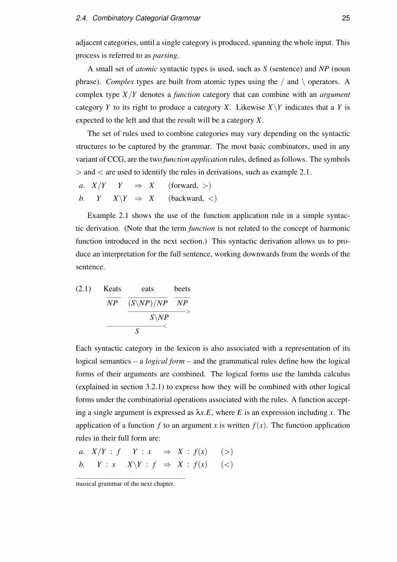
2.4. Combinatory Categorial Grammar 25
adjacent categories, until a single category is produced, spanning the whole input. This
process is referred to as parsing.
A small set of atomic syntactic types is used, such as S (sentence) and NP (noun
phrase). Complex types are built from atomic types using the / and \ operators. A
complex type X/Y denotes a function category that can combine with an argument
category Y to its right to produce a category X . Likewise X\Y indicates that a Y is
expected to the left and that the result will be a category X .
The set of rules used to combine categories may vary depending on the syntactic
structures to be captured by the grammar. The most basic combinators, used in any
variant of CCG, are the two function application rules, defined as follows. The symbols
> and < are used to identify the rules in derivations, such as example 2.1.
a. X/Y Y ⇒ X (forward, >)
b. Y X\Y ⇒ X (backward, <)
Example 2.1 shows the use of the function application rule in a simple syntac-
tic derivation. (Note that the term function is not related to the concept of harmonic
function introduced in the next section.) This syntactic derivation allows us to pro-
duce an interpretation for the full sentence, working downwards from the words of the
sentence.
(2.1) Keats eats beets
NP (S\NP)/NP NP>
S\NP<
S
Each syntactic category in the lexicon is also associated with a representation of its
logical semantics – a logical form – and the grammatical rules define how the logical
forms of their arguments are combined. The logical forms use the lambda calculus
(explained in section 3.2.1) to express how they will be combined with other logical
forms under the combinatorial operations associated with the rules. A function accept-
ing a single argument is expressed as λx.E, where E is an expression including x. The
application of a function f to an argument x is written f (x). The function application
rules in their full form are:
a. X/Y : f Y : x ⇒ X : f (x) (>)
b. Y : x X\Y : f ⇒ X : f (x) (<)
musical grammar of the next chapter.
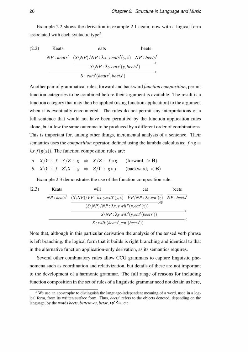
26 Chapter 2. Structure in Language and Music
Example 2.2 shows the derivation in example 2.1 again, now with a logical form
associated with each syntactic type3.
(2.2) Keats eats beets
NP : keats′ (S\NP)/NP : λx,y.eats′(y,x) NP : beets′>
S\NP : λy.eats′(y,beets′)<
S : eats′(keats′,beets′)
Another pair of grammatical rules, forward and backward function composition, permit
function categories to be combined before their argument is available. The result is a
function category that may then be applied (using function application) to the argument
when it is eventually encountered. The rules do not permit any interpretations of a
full sentence that would not have been permitted by the function application rules
alone, but allow the same outcome to be produced by a different order of combinations.
This is important for, among other things, incremental analysis of a sentence. Their
semantics uses the composition operator, defined using the lambda calculus as: f ◦g≡λx. f (g(x)). The function composition rules are:
a. X/Y : f Y/Z : g ⇒ X/Z : f ◦g (forward, > B)
b. X\Y : f Z\X : g ⇒ Z/Y : g◦ f (backward, < B)
Example 2.3 demonstrates the use of the function composition rule.
(2.3) Keats will eat beets
NP : keats′ (S\NP)/V P : λx,y.will′(y,x) V P/NP : λz.eat ′(z) NP : beets′>B
(S\NP)/NP : λx,y.will′(y,eat ′(x))>
S\NP : λy.will′(y,eat ′(beets′))<
S : will′(keats′,eat ′(beets′))
Note that, although in this particular derivation the analysis of the tensed verb phrase
is left branching, the logical form that it builds is right branching and identical to that
in the alternative function application-only derivation, as its semantics requires.
Several other combinatory rules allow CCG grammars to capture linguistic phe-
nomena such as coordination and relativization, but details of these are not important
to the development of a harmonic grammar. The full range of reasons for including
function composition in the set of rules of a linguistic grammar need not detain us here,
3 We use an apostrophe to distinguish the language-independent meaning of a word, used in a log-ical form, from its written surface form. Thus, beets’ refers to the objects denoted, depending on thelanguage, by the words beets, betteraves, betor, teÔtla, etc.
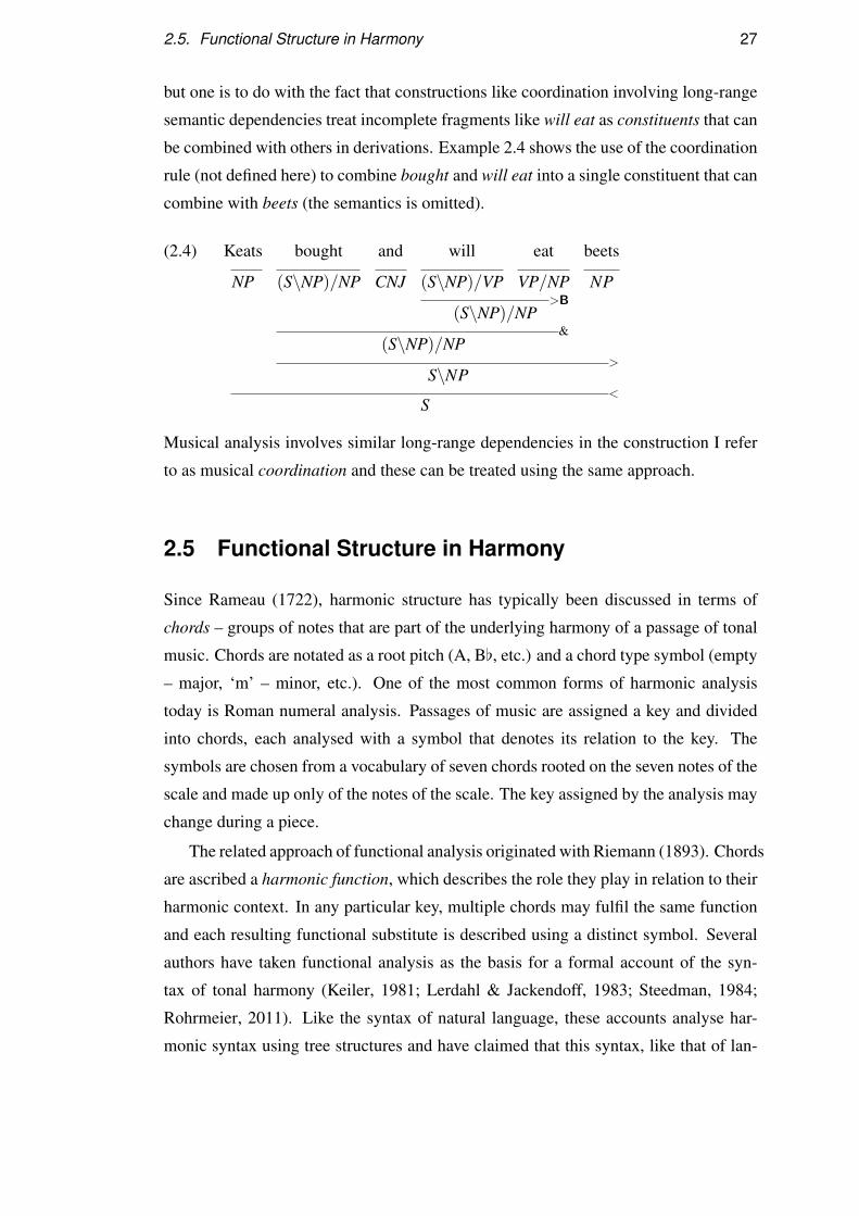
2.5. Functional Structure in Harmony 27
but one is to do with the fact that constructions like coordination involving long-range
semantic dependencies treat incomplete fragments like will eat as constituents that can
be combined with others in derivations. Example 2.4 shows the use of the coordination
rule (not defined here) to combine bought and will eat into a single constituent that can
combine with beets (the semantics is omitted).
(2.4) Keats bought and will eat beets
NP (S\NP)/NP CNJ (S\NP)/VP VP/NP NP>B
(S\NP)/NP&
(S\NP)/NP>
S\NP<
S
Musical analysis involves similar long-range dependencies in the construction I refer
to as musical coordination and these can be treated using the same approach.
2.5 Functional Structure in Harmony
Since Rameau (1722), harmonic structure has typically been discussed in terms of
chords – groups of notes that are part of the underlying harmony of a passage of tonal
music. Chords are notated as a root pitch (A, B[, etc.) and a chord type symbol (empty
– major, ‘m’ – minor, etc.). One of the most common forms of harmonic analysis
today is Roman numeral analysis. Passages of music are assigned a key and divided
into chords, each analysed with a symbol that denotes its relation to the key. The
symbols are chosen from a vocabulary of seven chords rooted on the seven notes of the
scale and made up only of the notes of the scale. The key assigned by the analysis may
change during a piece.
The related approach of functional analysis originated with Riemann (1893). Chords
are ascribed a harmonic function, which describes the role they play in relation to their
harmonic context. In any particular key, multiple chords may fulfil the same function
and each resulting functional substitute is described using a distinct symbol. Several
authors have taken functional analysis as the basis for a formal account of the syn-
tax of tonal harmony (Keiler, 1981; Lerdahl & Jackendoff, 1983; Steedman, 1984;
Rohrmeier, 2011). Like the syntax of natural language, these accounts analyse har-
monic syntax using tree structures and have claimed that this syntax, like that of lan-
28 Chapter 2. Structure in Language and Music
guage, features formally unbounded embedding of structural elements. I give here an
introduction to the aspects of harmonic structure that will be modelled later using for-
mal grammars. The functional view of harmonic structure adopted here has its roots in
the Euler-Riemannian tradition (Riemann, 1893) and closely follows the approaches
to harmonic analysis of Keiler, Steedman and Rohrmeier.
The functional harmonic analysis presented here is concerned only with the re-
lationships between chords which raise harmonic expectation and those which fulfil
that expectation. Huron (2006) discusses this and other forms of expectation in mu-
sic. Tonal expectation, that of relevance here, is described as a cognitive, rather than
perceptual, phenomenon. The structures analysed here are thus relevant to a descrip-
tion of musical perception, but the relationship between the cognitive structures that
underly human interpretation of harmony and perceptual responses is not simple. To
make predictions regarding listener responses to music on the basis of the theory of
cognition of harmony adopted here would additionally require a theory of incremen-
tal processing, taking account of working memory limitations. In particular, no direct
connection can be drawn between cognitive structures describing the final state of a
listener’s understanding and immediate perceptual responses during listening, as dis-
cussed in section 2.2.3.1. Naturally, harmonic expectation is only one aspect of music
contributing to a listener’s perception. Such predictions would, therefore, also rest on
a theory of the contributions of other aspects of music to the listener’s responses and
how these interact with the processing of harmonic structure. These issues are outside
the scope of the present thesis.
2.5.1 The Cadence and Harmonic Function
The key component of harmonic structure is the cadence, built from tension-resolution
patterns between chords. Large structures can be analysed as extended cadences, made
up of successive tension-resolution patterns chained together. The sort of harmonic
analysis that is described below captures the same relationships described by, among
others, Keiler (1981) and Rohrmeier (2011). The term cadence will be used throughout
this thesis to refer to all connected structures of tension-resolution patterns and never
in the more common sense of a particularly strong resolution that by convention marks
the end of a musical line or section.
Cadences come in two varieties. The authentic (or perfect) cadence consists of a
tension chord rooted a perfect fifth (or seven semitones, in equal temperament) above

2.5. Functional Structure in Harmony 29
CA7
D7G7 C
Figure 2.1: An extended authentic cadence in the key of C, a typical example of (tail)
recursion in music. The A7 acts as a dominant resolving to the D7, which in turn resolves
by the same relation to G7, which then resolves to the tonic C.
its resolution. This type of tension chord is defined in relation to its resolution as
having a dominant function. The plagal cadence consists of a tension chord rooted
a perfect fourth (five semitones) above its resolution. This type of tension chord is
referred to in relation to its resolution as having a subdominant function. In both cases,
the resolution chord is classified as a tonic chord in relation to the tension chord. The
classification of a particular occurrence of a chord identifies its harmonic function on
that occasion of use. The function of any particular chord is ambiguous and the same
chord may take on a different function on different occasions of use in the same piece.
An extended cadence occurs when a tension chord resolves by the appropriate in-
terval to a chord that is itself cadential, creating a further tension, which subsequently
resolves. Such a definition is recursive and extended cadences can accordingly be in-
definitely extended. An example is shown in the form of a tree in figure 2.1. Note
that, in terms of harmonic function as defined above, the G7 functions as a dominant
in relation to its resolution C and also as a tonic in relation to the dominant D7 chord4.
Chords that function as dominants are often partially, though never unambiguously,
distinguished by the addition of notes to the chord. In particular, the dominant sev-
enth, realized by the addition of the note a tone below the chord’s root and notated in
chord types with a superscript 7 (as in G7 above), enhances the cadential function of a
dominant chord and heightens the expectation of the corresponding tonic5. However,
this note may be omitted from a dominant chord, or may even be used in chords not
functioning as dominants. There is no similar signal of subdominant function in the
realization of the chords.
In certain contexts, one chord can be used in place of another with a different root
and fulfil the same harmonic function, a phenomenon referred to as chord substitution.
4 The D7 would often be referred to as a secondary dominant. I will use the term dominant to includesuch secondary harmonic function as well as further levels of recursion, or extended dominant where itis necessary to distinguish the recursive phenomenon from a chord with primitive dominant function.
5 The reasons for this are discussed by Steedman (1996) in terms of the tonal theory described below.

30 Chapter 2. Structure in Language and Music
C
&
D7G7 t A7
D7G7 t
t
C
Figure 2.2: An extended authentic cadence featuring coordination, marked here by &.
The shared resolution is marked by a trace symbol t.
In some cases, this can be explained by reference to notes shared between the two
chords, whilst in others it is less clear why a substitution attested by conventional
music practice works as it does. An example of a commonly used substitution is the
tritone substitution, by which a dominant seventh chord appears in place of another
dominant seventh chord rooted three tones above it.
2.5.2 Coordination
A tension chord might not reach its resolution immediately. An unresolved authen-
tic (or plagal) cadence, such as D7 G7, creating an expectation of tonic C, may be
interrupted by a further cadence, say A7 D7 G7, creating the same expectation, where-
upon both expectations/tensions will be resolved by the same tonic C. This cadence
structure is shown as a tree in figure 2.2. I refer to this operation as coordination by
virtue of its similarity to a type of coordination (right-node raising coordination) in
natural language sentences like Keats bought and will eat beets (see the derivation in
example 2.4). A coordinated cadence may itself be embedded in another coordinated
cadence, just as in examples like Keats ((may or may not) have bought) but (certainly
eats) beets. An example of a cadence with several levels of embedded coordination
can be seen in the form of a dependency graph in figure 3.5 in the next chapter.
2.5.3 Jazz Harmony
The typical size and complexity of cadence structures varies with musical period, genre
and composer. The type of harmonic structure discussed above developed with and
was permitted by the tonal system described in detail below and complex structures
2.6. Tonality 31
came about only with the wide acceptance of the equally tempered scale (see sec-
tion 2.6.3). Much previous work on computational music analysis has focused on
genres in which complex extended cadences are rare, such as folk music (Bod, 2002a;
Temperley, 2007) or common practice Western art music (Raphael & Stoddard, 2004).
Tonal jazz standards are of particular interest for the form of analysis described here
because they tend to feature large extended cadences, often with complex embedding.
They also include known harmonic variations created using a well-established system
of harmonic substitutions, embellishments and simplifications.
Jazz standards are rarely transcribed as full scores, but are notated as a melody with
an accompanying chord sequence, such as those analysed in the previous section. Iden-
tification of the times at which chords change in a piece of music and some character-
ization of the chords is usually the first step in harmonic analysis, even when chord la-
bels are not available on a score. The transcribed chord sequences of jazz standards al-
low us to begin defining a grammar of the syntax of tonal harmony by sidestepping the
issue of how this initial analysis is performed. It is an assumption of this approach that
the chord sequences provide a useful approximation to an intermediate analysis that
would necessarily feature in the harmonic analysis of musical performances. In chap-
ter 6 we shall see how a chord-based analysis may provide a starting point for an analy-
sis that incorporates this first phase of analysis in order to operate on performance data.
2.6 Tonality
2.6.1 Consonance and Harmony
In analysing the roles of pitch in music, it is important to distinguish between con-
sonance and harmony. Consonance is the sweetness or harshness of the sound that
results from playing two or more notes together. Harmony refers to the expectation
(or tension) created by particular combinations of notes and the satisfaction of that
expectation (or resolution of the tension)6. Both of these relations over pitches are
determined by small whole-number ratios and are easily confused, but arise in quite
different ways.
6 The word tension in this context refers to a specific type of musical tension associated with har-monic expectation (Huron, 2006). Contrasting consonance and dissonance also create a tension of adifferent sort. A further notion of tension is invoked by Lerdahl (2001), which relates more closely tothe perceived response by a listener and should not be confused with the specific harmonic tension inquestion here.

32 Chapter 2. Structure in Language and Music
The modern understanding of consonance originates with Helmholtz (1862), who
explained the phenomenon in terms of the coincidence and proximity of the secondary
overtones and difference tones that arise when simultaneously sounded notes excite
real non-linear physical resonators, including the human ear itself. These tones include
all integer multiples (and, in some cases, dividends) of the fundamental frequency.
Whilst the coincidence of lower ratios in general has a greater effect than higher on
consonance, there is no limit on the ratios that account for consonance. Helmholtz
(1862) describes first the physical principles that explain and characterize consonance.
He then formalizes the Western harmonic tonal system in terms of some related prin-
ciples, which we shall see below. Helmholtz is at pains to stress the importance of
distinguishing the naturally arising phenomenon of consonance from the relations that
exist between the notes of the tonal system (his italics):
Hence it follows,—and the proposition is not even now sufficientlypresent to the minds of our musical theoreticians and historians—that thesystem of Scales, Modes, and Harmonic Tissues does not rest solely uponinalterable natural laws, but is also, at least partly, the result of estheticalprinciples, which have already changed, and will still further change, withthe progressive development of humanity.
(Helmholtz, 1862, chapter XIII)
Harmonic analysis depends on a theory of tonality, which is concerned with the re-
lations between notes in the tonal system. The issue of consonance is largely irrelevant
to this, except in so far as it bears upon a historical description of the system’s devel-
opment. These two aspects of music both contribute to the same musical surface form
and but are commonly treated as theoretically distinct. Other aspects of music that
contribute to the same surface form, such as voice-leading, are likewise distinguished
on theoretical grounds. A listener’s perception of and responses to music are often a
result of a combination of different aspects of music supposed to require the cognition
of separate musical structures. The experiments of Krumhansl (1990) concern the hu-
man responses that result from this combination and thus incorporate issues of both
harmony and consonance. Johnson-Laird et al. (2012) attempt to account for a notion
of perceived dissonance by explicit combination of two distinct models. Unlike these
authors, I shall pass over the issue of consonance in the following description of tonal
theory. The present thesis is concerned only with the analysis of the structure of har-
mony, without any attempt to combine this, in the manner of Johnson-Laird et al., with
a model of other aspects of musical cognition to make predictions about a listener’s
perception.

2.6. Tonality 33
G[[
B[[
D[
F
A
C]
D[[
F[
A[
C
E
G]
A[[
C[
E[
G
B
D]
E[[
G[
B[
D
F]
A]
B[[
D[
F
A
C]
E]
F[
A[
C
E
G]
B]
C[
E[
G
B
D]
F]]
G[
B[
D
F]
A]
C]]
D[
F
A
C]
E]
G]]
A[
C
E
G]
B]
D]]
E[
G
B
D]
F]]
A]]
Figure 2.3: Part of the space of note names (Longuet-Higgins, 1962a,b). The circles
mark two points separated by the syntonic comma, the squares two points separated
by the diesis.
2.6.2 Just Intonation
Like the theory of consonance, the tonal harmonic system derives from combinations
of small integer pitch ratios. However, the harmonic relation is based solely on the first
three prime ratios in the harmonic series: ratios of 2, 3 and 5 (the octave, perfect fifth
and major third). The tuning based on these exact intervals is known as just intonation.
Any interval between two notes in just intonation corresponds to a frequency ra-
tio defined as the product 2x · 3y · 5z, where x,y,z are positive or negative integers. It
has been observed since Euler (1739) that the harmonic relation can, therefore, be vi-
sualized as an infinitely extending, discrete, three-dimensional space with these three
prime factors as generators. Since notes separated by octaves are essentially equivalent
for tonal purposes, it is convenient to project the space onto the 3,5 plane. The presen-
tation of this theory that is adopted here, which will later form the basis for harmonic
analysis, was originally developed by Ellis (1874) and formally developed in the form
it is seen here by Longuet-Higgins (1962a,b).
A fragment of the space can be seen in figure 2.3. Conventional musical notation,
by which the points in the space are named, does not distinguish notes separated by
the interval corresponding to the vector (4,−1), the so-called syntonic comma (for
example between the two Cs marked by circles in figure 2.3). Notes separated by the
much larger diesis, (3,0), have distinct names (for example G] and A[, marked by
squares) and are referred to as enharmonic tones. The points in figure 2.4 represent
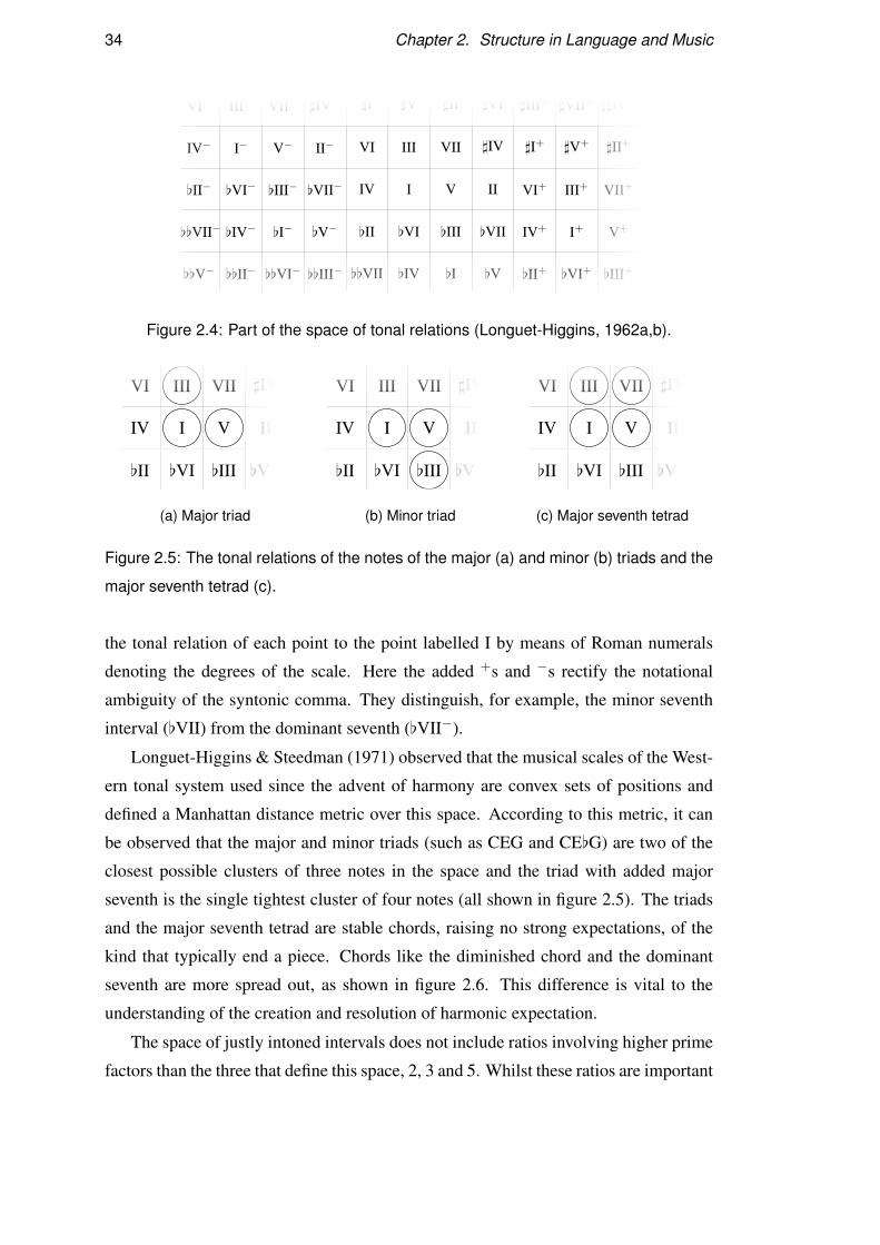
34 Chapter 2. Structure in Language and Music
[[V−
[[VII−
[II−
IV−
VI−
[[II−
[IV−
[VI−
I−
III−
[[VI−
[I−
[III−
V−
VII−
[[III−
[V−
[VII−
II−
]IV−
[[VII
[II
IV
VI
]I
[IV
[VI
I
III
]V
[I
[III
V
VII
]II
[V
[VII
II
]IV
]VI
[II+
IV+
VI+
]I+
]III+
[VI+
I+
III+
]V+
]VII+
[III+
V+
VII+
]II+
]]IV+
Figure 2.4: Part of the space of tonal relations (Longuet-Higgins, 1962a,b).
[II
IV
VI
[VI
I
III
[III
V
VII
[VII
II
]IV
(a) Major triad
[II
IV
VI
[VI
I
III
[III
V
VII
[VII
II
]IV
(b) Minor triad
[II
IV
VI
[VI
I
III
[III
V
VII
[VII
II
]IV
(c) Major seventh tetrad
Figure 2.5: The tonal relations of the notes of the major (a) and minor (b) triads and the
major seventh tetrad (c).
the tonal relation of each point to the point labelled I by means of Roman numerals
denoting the degrees of the scale. Here the added +s and −s rectify the notational
ambiguity of the syntonic comma. They distinguish, for example, the minor seventh
interval ([VII) from the dominant seventh ([VII−).
Longuet-Higgins & Steedman (1971) observed that the musical scales of the West-
ern tonal system used since the advent of harmony are convex sets of positions and
defined a Manhattan distance metric over this space. According to this metric, it can
be observed that the major and minor triads (such as CEG and CE[G) are two of the
closest possible clusters of three notes in the space and the triad with added major
seventh is the single tightest cluster of four notes (all shown in figure 2.5). The triads
and the major seventh tetrad are stable chords, raising no strong expectations, of the
kind that typically end a piece. Chords like the diminished chord and the dominant
seventh are more spread out, as shown in figure 2.6. This difference is vital to the
understanding of the creation and resolution of harmonic expectation.
The space of justly intoned intervals does not include ratios involving higher prime
factors than the three that define this space, 2, 3 and 5. Whilst these ratios are important
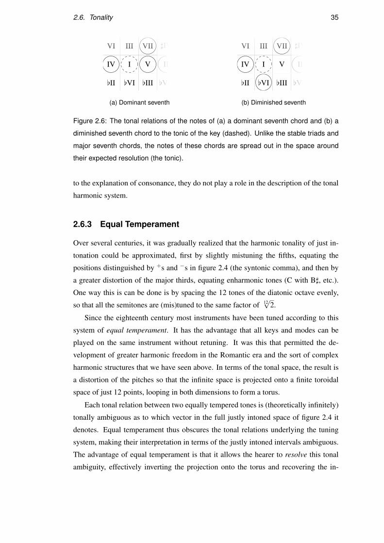
2.6. Tonality 35
[II
IV
VI
[VI
I
III
[III
V
VII
[VII
II
]IV
(a) Dominant seventh
[II
IV
VI
[VI
I
III
[III
V
VII
[VII
II
]IV
(b) Diminished seventh
Figure 2.6: The tonal relations of the notes of (a) a dominant seventh chord and (b) a
diminished seventh chord to the tonic of the key (dashed). Unlike the stable triads and
major seventh chords, the notes of these chords are spread out in the space around
their expected resolution (the tonic).
to the explanation of consonance, they do not play a role in the description of the tonal
harmonic system.
2.6.3 Equal Temperament
Over several centuries, it was gradually realized that the harmonic tonality of just in-
tonation could be approximated, first by slightly mistuning the fifths, equating the
positions distinguished by +s and −s in figure 2.4 (the syntonic comma), and then by
a greater distortion of the major thirds, equating enharmonic tones (C with B], etc.).
One way this is can be done is by spacing the 12 tones of the diatonic octave evenly,
so that all the semitones are (mis)tuned to the same factor of 12√
2.
Since the eighteenth century most instruments have been tuned according to this
system of equal temperament. It has the advantage that all keys and modes can be
played on the same instrument without retuning. It was this that permitted the de-
velopment of greater harmonic freedom in the Romantic era and the sort of complex
harmonic structures that we have seen above. In terms of the tonal space, the result is
a distortion of the pitches so that the infinite space is projected onto a finite toroidal
space of just 12 points, looping in both dimensions to form a torus.
Each tonal relation between two equally tempered tones is (theoretically infinitely)
tonally ambiguous as to which vector in the full justly intoned space of figure 2.4 it
denotes. Equal temperament thus obscures the tonal relations underlying the tuning
system, making their interpretation in terms of the justly intoned intervals ambiguous.
The advantage of equal temperament is that it allows the hearer to resolve this tonal
ambiguity, effectively inverting the projection onto the torus and recovering the in-

36 Chapter 2. Structure in Language and Music
G 44ˇ 3ˇ 4ˇ ˇ 2 ˇ > ˇ ˘
1
Figure 2.7: “Shave and a haircut, six bits”.
terpretation of the intervals in the full harmonic space. This is possible because the
harmonic intervals that are sufficiently close in justly intoned frequency to be equated
on the equally tempered torus are sufficiently distant in the full space for the musical
context to disambiguate them. For example, beginning from a G, an equally tempered
C, which could in isolation be interpreted as any of the points labelled as C or one of its
enharmonic equivalents (five possibilities are visible in figure 2.3), must be interpreted
as the point immediately to the left of the G, because that is the only interpretation that
is anywhere close to G.
It has often been claimed (Jeans, 1937; Bernstein, 1976; Tymoczko, 2006) that
the dominant seventh (the leftmost note in the cluster in figure 2.6a) played in equal
temperament approximates a tone based on the seventh harmonic (that is, a ratio of 7 :
4). Such a claim confuses the tonal harmonic relation, situated in the three-dimensional
system above, with consonance. In the tonal system, an equally tempered B[ may
be interpreted as related to C by either a dominant seventh ([VII− in figure 2.4) or
a minor seventh ([VII). The similarity of the equally tempered interval (21012 ) to the
seventh harmonic (74 ) provides no grounds for the addition of a fourth dimension to
the tonal space, since no combination of the interval with the other generators, or even
with itself, is proposed. This argument applies to the Western tonal harmonic system
only. Varieties of music other than those that use the harmonically motivated tonality
described here might take 7 : 4 as a primitive ratio, although it is doubtful that such a
music could support equal temperament or even a very extensive form of harmony.
2.6.4 Harmonic Interpretation
We are now able to define a more precise notion of harmonic interpretation, expressed
in terms of the theory of harmonic tonality outlined above. A harmonic interpretation,
as performed unconsciously by a listener familiar with the tonal system, can be seen
as a projection of the notes and the underlying chord roots of a piece of music from
the 4×3 space of equal temperament onto the infinite space of tonal relations. It is by
recognizing the tonal relations underlying the equally tempered music that a listener
can identify the key in which the music is played.

2.6. Tonality 37
0
4
8
0
4
7
11
3
7
11
2
6
10
2
6
9
1
5
9
1
4
8
0
4
8
11
3
7
11
3
6
10
2
6
10
1
5
9
1
5
8
0
4
8
0
Figure 2.8: Part of the tonal space labelled according to its projection under equal
temperament onto 12 distinct pitches (Longuet-Higgins & Steedman, 1971).
Let us consider the simple musical example shown in figure 2.7, a cliche of a
melodic conclusion (first used in this context by Longuet-Higgins, 1979). The passage
divides naturally into two parts, corresponding to the two bars as it is notated here. The
first moves in the underlying harmonic progression from the tonic C to the dominant
G, whilst the second returns to the tonic. The first movement, in the second half bar,
to the dominant creates an expectation of a cadential return to the tonic. The second
bar satisfies this expectation, albeit a little later than would seem natural, only reaching
the tonic in the second half of the bar. It is easy to verify this analysis by playing the
melody with accompanying chords: a triad of C major and a triad of G major (with
added dominant seventh). Although the score includes only a melody, a crucial part of
understanding its meaning even when it is performed alone is an unconscious analysis
by the listener of the implicit harmony.
Consider the tonal space shown in figure 2.8, labelled as by Longuet-Higgins &
Steedman (1971) using numbers to refer to the notes of an equally tempered keyboard
(C=0, C]=D[=1, etc.). We can express the above harmonic analysis of figure 2.7 in
terms of the movement of the underlying chord root in the space. The passage begins
on C, let us say the central point labelled 0 (circled). Halfway through the first bar it
moves to the G (7) one step to the right. Halfway through the second bar, it steps back
to the left to land on C (0) again. Equal temperament obscures the distinction between
the tone labelled 7 marked in figure 2.8 and all other 7s. The disambiguation in this
case, however, is trivial. The G is interpreted as a dominant in the key established by
the C (outlined) and is, therefore, at the adjacent position. Likewise, the C to which
the dominant resolves must be that immediately to the left of it.
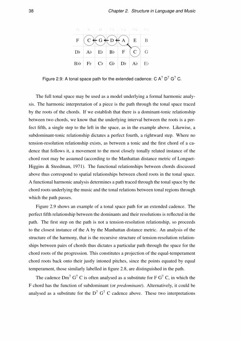
38 Chapter 2. Structure in Language and Music
B[[
D[
F
A
F[
A[
C
E
C[
E[
G
B
G[
B[
D
F]
D[
F
A
C]
A[
C
E
G]
E[
G
B
D]
Figure 2.9: A tonal space path for the extended cadence: C A7 D7 G7 C.
The full tonal space may be used as a model underlying a formal harmonic analy-
sis. The harmonic interpretation of a piece is the path through the tonal space traced
by the roots of the chords. If we establish that there is a dominant-tonic relationship
between two chords, we know that the underlying interval between the roots is a per-
fect fifth, a single step to the left in the space, as in the example above. Likewise, a
subdominant-tonic relationship dictates a perfect fourth, a rightward step. Where no
tension-resolution relationship exists, as between a tonic and the first chord of a ca-
dence that follows it, a movement to the most closely tonally related instance of the
chord root may be assumed (according to the Manhattan distance metric of Longuet-
Higgins & Steedman, 1971). The functional relationships between chords discussed
above thus correspond to spatial relationships between chord roots in the tonal space.
A functional harmonic analysis determines a path traced through the tonal space by the
chord roots underlying the music and the tonal relations between tonal regions through
which the path passes.
Figure 2.9 shows an example of a tonal space path for an extended cadence. The
perfect fifth relationship between the dominants and their resolutions is reflected in the
path. The first step on the path is not a tension-resolution relationship, so proceeds
to the closest instance of the A by the Manhattan distance metric. An analysis of the
structure of the harmony, that is the recursive structure of tension-resolution relation-
ships between pairs of chords thus dictates a particular path through the space for the
chord roots of the progression. This constitutes a projection of the equal-temperament
chord roots back onto their justly intoned pitches, since the points equated by equal
temperament, those similarly labelled in figure 2.8, are distinguished in the path.
The cadence Dm7 G7 C is often analysed as a substitute for F G7 C, in which the
F chord has the function of subdominant (or predominant). Alternatively, it could be
analysed as a substitute for the D7 G7 C cadence above. These two interpretations

2.6. Tonality 39
correspond to distinct analyses of the tonal relations between chord roots, as can be
seen in the corresponding tonal space path. The cadence is ambiguous: it supports
both of these interpretations. In jazz, such a cadence may be, and often is, extended
with recursive dominant-function chords. In these extended cadences, 7 and m7 chords
may be freely substituted without constituting a change to the functional structure of
the harmony. Where a recursive dominant relation is extended in this way, as in the
cadence E7 A7 Dm7 G7 C, only an analysis of the Dm7 as being followed by a left
step in the tonal space presents a satisfactory explanation of the presence of the out-of-
key chords E7 and A7 (by the recursive dominant relation). This type of recursion is
very common in jazz. Consequently, the examples in this thesis will employ the latter
interpretation, accepting that the former may be equally acceptable in some cases.
2.6.5 Example Interpretations
I present here several examples of harmonic interpretations expressed in terms of the
movements of chord roots through the tonal space. The next chapter introduces a
language to describe just such interpretations as these in a form that can be built up
compositionally from interpretations of individual chords.
Basin Street Blues Louis Armstrong
This song, in the key of B[, has a long introduction, mostly on a B[ chord. As is
usual in jazz standards, this is followed by a head, which may be repeated indefinitely
and improvised over. The repeated chords in the head are shown in example 2.5, with
their tonal space analysis.
(2.5) B[ D7 G7 A[6 G7 C9 F7 B[
A[[
C[
E[
G
E[[
G[
B[
D
B[[
D[
F
A
F[
A[
C
E
C[
E[
G
B
G[
B[
D
F]
D[
F
A
C]
Note first the use of the tritone substitution. The fourth chord, A[6 is analysed as a
substitution in place of a D7. The tonal space analysis does not include a A[: this
chord corresponds instead to the rightward movement from G back to the D.

40 Chapter 2. Structure in Language and Music
What makes this chord sequence interesting is that the final resolution of the ca-
dence to a tonic on B[ is shown in the analysis to be the point a row above and four
steps to the left of where we began. This is because the cadence contains enough re-
cursive dominants, which must be analysed as leftward steps, that its starting point is
closer to another instance of B[ than the one it resolves to. The transition from the
initial tonic to the start of the cadence (D7) is taken to be by the closest possible tonal
relation – a major third.
This sort of trickery is permitted by equal temperament. If the piece were per-
formed on a justly intoned instrument with fixed tuning, a distortion of the perfect fifth
would be heard between the G7 and C9. If it were performed on a justly intoned in-
strument capable of adjusting its tuning during a performance7, the result would be a
gradual, but noticeable, drop in pitch with each repetition.
Prelude No. 1 (from Eight Short Preludes and Fugues) J. S. Bach
I have previously presented an analysis (Wilding, 2008) of the first prelude from
J. S. Bach’s Eight Short Preludes and Fugues (BWV 553–560) using the categories
of an earlier development of the musical syntactic formalism described in the next
chapter. The opening section is reproduced below.
�
���
�
�
��� �
��� ���
�����
������
��
���� �
�
�
�
�
��� �
�
� ��
� �� ���
�
�
�
�
� � ��
���
��
�� �
�
mf� � ����� � � �
�
��
�
�� �
�
�
�
�����
�
��
� � ��
�
�
�
���
�
�4
��
�
��� �
����
�
�
����� �� �
�
�
���
� � �� ����
�
�
�
���
�
�� �
�
�
�
� ���
�
���
�
�
�
����
�
����
� �
�
�
����
� �����
�
���
�
���
�
��� ��
��
�
�
�
�
���
�
��� ��
�
����
��
�
��
�
�����
��
7
���� �
�
���
����� �
����
���
�
���� �
��
�
��
�
���
�
��� �
��
�
�� �
�
���
�
���
��
�
� ���
�
������
��
�
�
�
���� �
�
����
7 Thanks to modern technology, this is in fact possible nowadays, even without the services of Ellis’obliging London harmonium manufacturer (Helmholtz, 1862).

2.6. Tonality 41
��
��
��
��
�
�
���
�
��
�
��
����� �
�
����
�
���
10
�
�
�
��
��� �
�
�
��� �
��
���
���
�����
�
�
���
�
��
�
�
�
�
� ��
�����
� �� � ����
� ��
�
�
�
�
�
�
�
��
�
�
�
����
Unsurprisingly, given Bach’s enthusiasm for well temperaments (tuning systems
which, like equal temperament, approximate just intonation in a way that permits free
key changes), this short passage moves through an extraordinary sequence of con-
nected tonalities that would have been impossible without contemporary tuning in-
novations. The tonal space analysis in example 2.6 is labelled with the bar and beat
numbers of the above score (in the form ‘bar.beat’). The function of a chord is made
clear by the voicing in many cases by presence of either a dominant seventh note (such
as the C in the first inversion D major chord of bar 3), implying a dominant function,
or a major seventh note (such as the F] of the G major chord that follows it), implying
a tonic function.
(2.6)
G[[
B[[
D[
F
A
D[[
F[
A[
C
E
A[[
C[
E[
G
B
E[[
G[
B[
D
F]
B[[
D[
F
A
C]
F[
A[
C
E
G]
C[
E[
G
B
D]
G[
B[
D
F]
A]
D[
F
A
C]
E]
A[
C
E
G]
B]
E[
G
B
D]
F]]
B[
D
F]
A]
C]]
F
A
C]
E]
G]]
1.12.3 3.13.3
4.14.35.15.36.1
6.37.17.38.18.3. . .9.1. . .1.1
The piece opens with one and a half bars of a C major chord, establishing the piece’s
main key. The F major chord at 2.3 is interpreted as a subdominant, since the major
seventh of the previous C chord deters us from treating it as a dominant in relation
to this F. Consequently, the D major (3.1) must be interpreted as that closest to the
opening tonality of C (rather than that above and left of the F). The dominant D resolves
to a new tonic G at 3.3. A dominant E at 4.1 resolves briefly to a new tonic again,
this time A minor. Bar 5 contains another dominant D to tonic G resolution and bar
6 returns us momentarily to the main key of C. Whilst the interpretation so far has
moved by pairs of dominant-tonic resolutions, notice that the tonic A is followed by
a dominant a perfect fifth below, D, and the tonic G by an unprepared tonic C, also
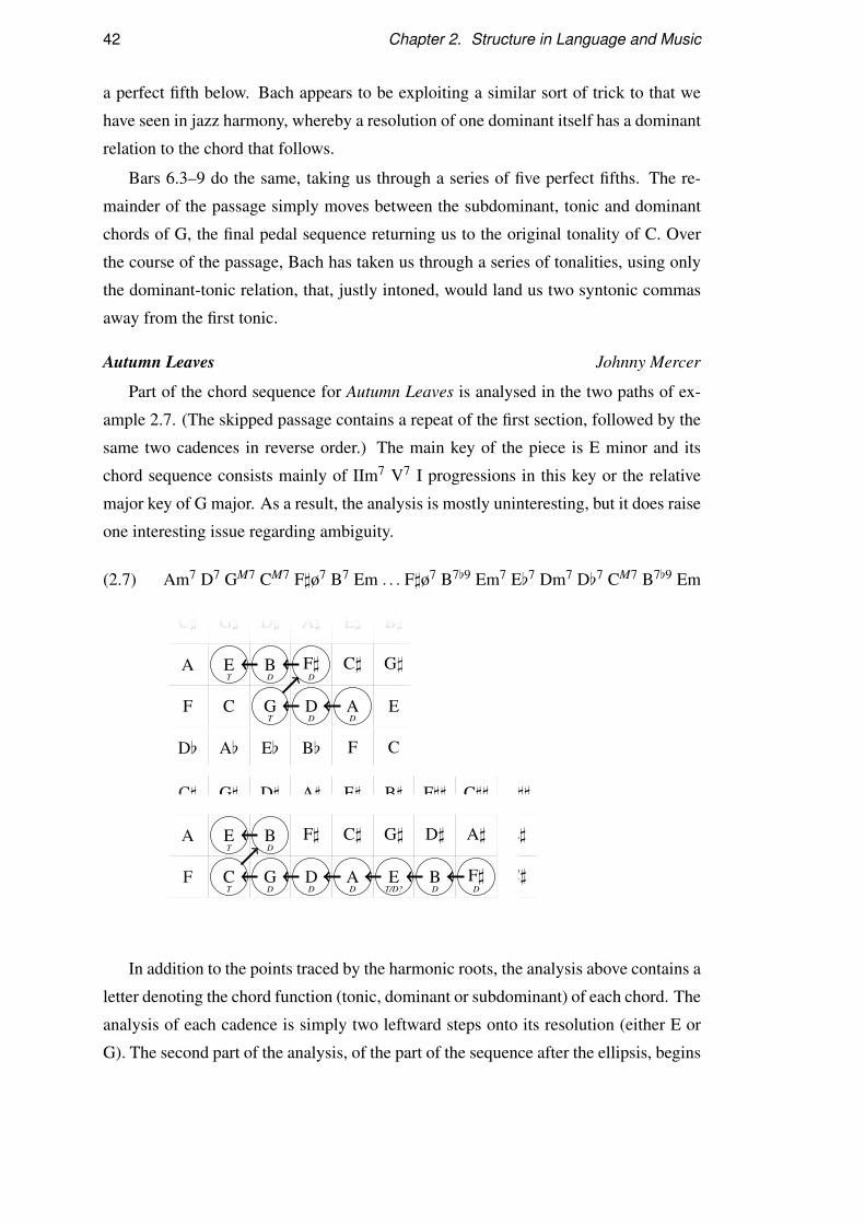
42 Chapter 2. Structure in Language and Music
a perfect fifth below. Bach appears to be exploiting a similar sort of trick to that we
have seen in jazz harmony, whereby a resolution of one dominant itself has a dominant
relation to the chord that follows.
Bars 6.3–9 do the same, taking us through a series of five perfect fifths. The re-
mainder of the passage simply moves between the subdominant, tonic and dominant
chords of G, the final pedal sequence returning us to the original tonality of C. Over
the course of the passage, Bach has taken us through a series of tonalities, using only
the dominant-tonic relation, that, justly intoned, would land us two syntonic commas
away from the first tonic.
Autumn Leaves Johnny Mercer
Part of the chord sequence for Autumn Leaves is analysed in the two paths of ex-
ample 2.7. (The skipped passage contains a repeat of the first section, followed by the
same two cadences in reverse order.) The main key of the piece is E minor and its
chord sequence consists mainly of IIm7 V7 I progressions in this key or the relative
major key of G major. As a result, the analysis is mostly uninteresting, but it does raise
one interesting issue regarding ambiguity.
(2.7) Am7 D7 GM7 CM7 F]ø7 B7 Em . . . F]ø7 B7[9 Em7 E[7 Dm7 D[7 CM7 B7[9 Em
D[
F
A
C]
A[
C
E
G]
E[
G
B
D]
B[
D
F]
A]
F
A
C]
E]
C
E
G]
B]
DDT
DDT
D[
F
A
C]
A[
C
E
G]
E[
G
B
D]
B[
D
F]
A]
F
A
C]
E]
C
E
G]
B]
G
B
D]
F]]
D
F]
A]
C]]
A
C]
E]
G]]
DDT/D?DDDT
DT
In addition to the points traced by the harmonic roots, the analysis above contains a
letter denoting the chord function (tonic, dominant or subdominant) of each chord. The
analysis of each cadence is simply two leftward steps onto its resolution (either E or
G). The second part of the analysis, of the part of the sequence after the ellipsis, begins

2.6. Tonality 43
F]ø7B7[9 Em7 E[7
Dm7D[7 CM7
(a)
F]ø7
B7[9
Em7
E[7
Dm7D[7 CM7
(b)
Figure 2.10: Two ways of interpreting a passage from Autumn Leaves: (a) as two
separate cadences; (b) as a single cadence, in which the Em7 has a dominant function.
with another cadence onto Em, which is followed by a long extended cadence onto C.
The cadence includes two tritone substitutions (E[7 and D[7), resulting in a sequence of
surface chord roots moving down in semitones. Two ways in which this passage could
be interpreted are as follows: as a cadence resolving to an E minor tonic followed by
another resolving to C major; or as a single cadence in which the Em7 chord functions
as an extended dominant resolving to E[7 (which is a tritone substitution for A7). The
only difference between the two interpretations in the tonal space analysis is in the
annotation of the E root as a tonic in the former case or a dominant in the latter. The
fact that many recordings of the song use a chord sequence that does not permit the
second interpretation of this passage, together with the chord types on the first three
chords typical of a minor cadence ending, suggests that we must interpret the Em7 as
a tonic. Nevertheless, when this particular sequence is used, it seems to be possible to
hear the Em7 chord also as a dominant participating in the next cadence. A third, and
perhaps more plausible, way of viewing the connection between the Em7 and E[7 in
this latter analysis is to treat the Em7 as having two functions: a tonic at the right edge
of the first subtree of figure 2.10a and a dominant at the left edge of the second. Such
double functions are represented in the analyses of Rohrmeier (2011).
This is an example of an ambiguity in interpretation: these readings can be dis-
tinguished in the tonal space path analysis, when harmonic functions are included,
allowing us to propose multiple different analyses, expressing both formally and mak-
ing explicit the difference between them in terms of the music theory that underlies
the analysis. Such ambiguities, featuring multiple plausible alternative readings, are
common in music and it is essential to a theory of harmonic structure that it be capable
of explaining precisely the differences between the alternative readings. A similar type
of ambiguity in natural language gives rise to multiple readings of sentences like two
sisters reunited after 18 years at checkout counter.
44 Chapter 2. Structure in Language and Music
2.7 Conclusion
This chapter has put the present thesis in the context of research in music cognition
and computational linguistics and laid out the theoretical background for the approach
taken in later chapters. Constructing models of the structure of tonal harmony is im-
portant both for modelling human cognition of music and for practical tasks in auto-
matic music processing. Formal grammars modelling syntactic processing of natural
language to produce semantic representations will form the basis for the approach to
formal harmonic analysis taken in the next chapter. In particular, the grammar formal-
ism of CCG will be adapted as appropriate to tonal analysis and the basic elements of
the formalism have been described here as they are applied to linguistic analysis.
The result of harmonic analysis is an identification of the tonal relationships be-
tween the chords of the musical material. This chapter has introduced the sorts of
structure formed by these relationships and related them to the interpretation of the
music in terms of the three-dimensional tonal space of Longuet-Higgins (1979). A
formalization of the two views of harmonic analysis introduced here – the decompo-
sition of the hierarchical structure of cadences and the corresponding path of chord
roots through the tonal space – will both be later treated as the output of the process of
automatic harmonic analysis and used as the basis for quantitative evaluation metrics.

CHAPTER 3A Grammar for Tonal Harmony
3.1 Introduction
The process of harmonic analysis involves the inference of tonal relations between the
chord roots underlying passages of a piece of music. As we have seen, in figure 2.2,
a particular analysis may specify the tonal relation between two chords that are not
adjacent in the musical surface. Given some formal language to express these rela-
tions, harmonic analysis becomes the process of mapping the musical surface onto an
expression in that language, or a set of possible expressions representing alternative
analyses. As in linguistics, a generalized mechanism for mapping the surface form to
its analysis can be characterized using a grammar. The grammar expresses the neces-
sary constraints on the types of constituents that can be combined during the analysis
process and the form of the resulting analysis.
Steedman (1996) proposed a small generative grammar, using an adaptation of
CCG to harmonic syntax, covering a narrow musical domain – chord sequences of
variations on the twelve-bar blues – and a formal language sufficient to express har-
monic interpretations of these chord sequences. The present author expanded both
the harmonic analysis language and the syntactic formalism to permit interpretation
of a wider range of chord sequences than just twelve-bar blues (Wilding, 2008). This
chapter presents some small further developments of the harmonic analysis language
45
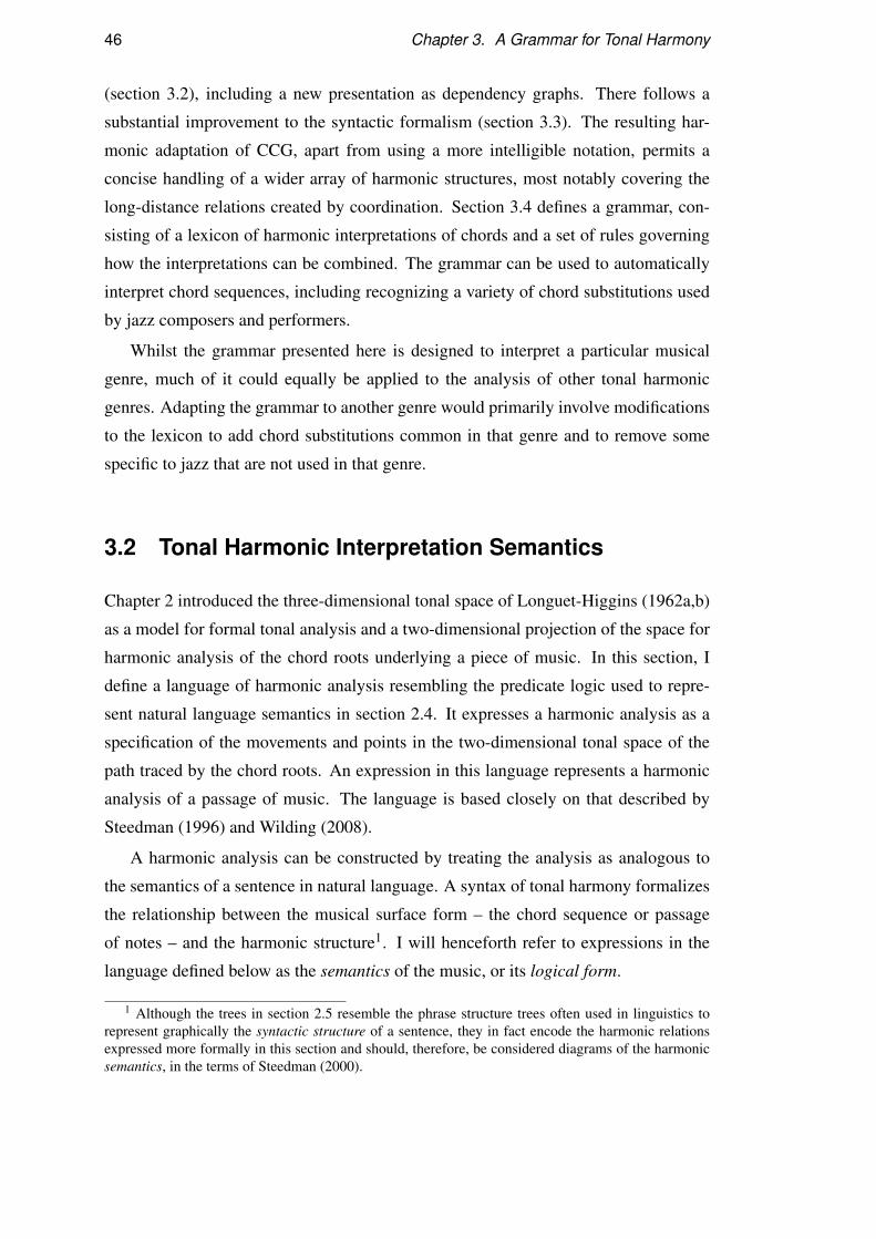
46 Chapter 3. A Grammar for Tonal Harmony
(section 3.2), including a new presentation as dependency graphs. There follows a
substantial improvement to the syntactic formalism (section 3.3). The resulting har-
monic adaptation of CCG, apart from using a more intelligible notation, permits a
concise handling of a wider array of harmonic structures, most notably covering the
long-distance relations created by coordination. Section 3.4 defines a grammar, con-
sisting of a lexicon of harmonic interpretations of chords and a set of rules governing
how the interpretations can be combined. The grammar can be used to automatically
interpret chord sequences, including recognizing a variety of chord substitutions used
by jazz composers and performers.
Whilst the grammar presented here is designed to interpret a particular musical
genre, much of it could equally be applied to the analysis of other tonal harmonic
genres. Adapting the grammar to another genre would primarily involve modifications
to the lexicon to add chord substitutions common in that genre and to remove some
specific to jazz that are not used in that genre.
3.2 Tonal Harmonic Interpretation Semantics
Chapter 2 introduced the three-dimensional tonal space of Longuet-Higgins (1962a,b)
as a model for formal tonal analysis and a two-dimensional projection of the space for
harmonic analysis of the chord roots underlying a piece of music. In this section, I
define a language of harmonic analysis resembling the predicate logic used to repre-
sent natural language semantics in section 2.4. It expresses a harmonic analysis as a
specification of the movements and points in the two-dimensional tonal space of the
path traced by the chord roots. An expression in this language represents a harmonic
analysis of a passage of music. The language is based closely on that described by
Steedman (1996) and Wilding (2008).
A harmonic analysis can be constructed by treating the analysis as analogous to
the semantics of a sentence in natural language. A syntax of tonal harmony formalizes
the relationship between the musical surface form – the chord sequence or passage
of notes – and the harmonic structure1. I will henceforth refer to expressions in the
language defined below as the semantics of the music, or its logical form.
1 Although the trees in section 2.5 resemble the phrase structure trees often used in linguistics torepresent graphically the syntactic structure of a sentence, they in fact encode the harmonic relationsexpressed more formally in this section and should, therefore, be considered diagrams of the harmonicsemantics, in the terms of Steedman (2000).

3.2. Tonal Harmonic Interpretation Semantics 47
Logical forms in this language are compositional: the logical form for a piece of
music can be composed from the logical forms of subsequences of the piece, using
a suitable syntax and using the lambda calculus to express gaps in the analysis that
will be filled by other partial logical forms. Thus individual chords can be assigned an
interpretation as a logical form, along with a syntactic type to constrain the ways this
can combine with the interpretation of other chords (see section 3.3). An interpretation
(or multiple interpretations) of the full piece can be produced by combining them, just
as the meaning of Keats will eat beets was built up from the meaning of its individual
words in example 2.3.
3.2.1 The Lambda Calculus as Notation
The lambda calculus provides a notation for expressing variable binding in functional
expressions.
Consider the semantics of example 2.2, reproduced in example 3.1:
(3.1) Keats eats beets
keats′ λx,y.eats′(y,x) beets′>
λy.eats′(y,beets′)<
eats′(keats′,beets′)
The predicate eats′ represents the action of eating, taking the agent (the eater) as its
first argument and the patient (the eaten) as its second. The semantics of eats is this
predicate, with gaps left for the arguments, marked by the variables x and y. Recall
that the > and < combinatorial rules (forward and backward function application) are
associated with the operation of function application in the semantics.
The lambda calculus allows us to bind a variable x in an expression, creating a
function which, when applied to an argument A, will return the same expression, but
with A substituted for every occurrence of x. The operation of binding a variable is
notated using λ and is referred to as lambda abstraction:
f = λx.E, where E may include x as a free variable
Where more than one variable is bound at the same time by immediate nesting of
lambda abstractions, only one λ is written, with comma-separated variable names:
f = λx,y.E
≡ λx.λy.E

48 Chapter 3. A Grammar for Tonal Harmony
In example 3.1, the lambda calculus allows us to build the semantics of eats as a
function which takes two arguments and produces a new logical form consisting of
the predicate eats′ applied to the function’s arguments (in reverse). The corresponding
syntactic category (S\NP)/NP ensures that the first argument to the function is the
patient of the action, in the object position (right of the verb in English), and the second
argument is the agent, in the subject position (left in English).
Example 3.2 shows how similar logical forms could be used in a passive construc-
tion to produce an identical interpretation of the whole sentence. The only difference
between the logical form for are eaten by here and eats above is the order of the vari-
ables as arguments to the predicate, now eats′(x,y) as opposed to eats′(y,x): the first
argument is now treated as the agent and the second as the patient.
(3.2) Beets are eaten by Keats
beets′ keats′λx,y.eats′(x,y)
>λy.eats′(keats′,y)
<eats′(keats′,beets′)
Using the lambda calculus to express variable binding in functions and a formal lan-
guage for the sort of harmonic interpretations described in section 2.6.4 will allow us
to associate partially formed harmonic interpretations with constituents of a harmonic
progression and compose them into an interpretation of the full progression.
3.2.2 Interpretation of Tonics
The semantics of a tonic chord is represented in a logical form as a point in the tonal
space which is constrained to be one that is mapped by equal temperament to the
chord’s root as written. This still permits a theoretically infinite set of points that could
be used to interpret the chord’s root. For an isolated tonic logical form, there is no
reason to constrain which of these points is chosen: its relation to other points in a full
logical form will be fully determined by constraints imposed by the rest of the logical
form. The logical form is a coordinate in a 4×3 enharmonic space identifying this
infinite set. The enharmonic space can be seen as the projection of the full tonal space
onto equal temperament, or equivalently as an infinite set of 4×3 subspaces in the tonal
space, as shown in figure 3.1. The notation 〈x,y〉 denotes an enharmonic coordinate, as
distinct from the coordinate or vector (x,y) in the full space. The coordinate, therefore,
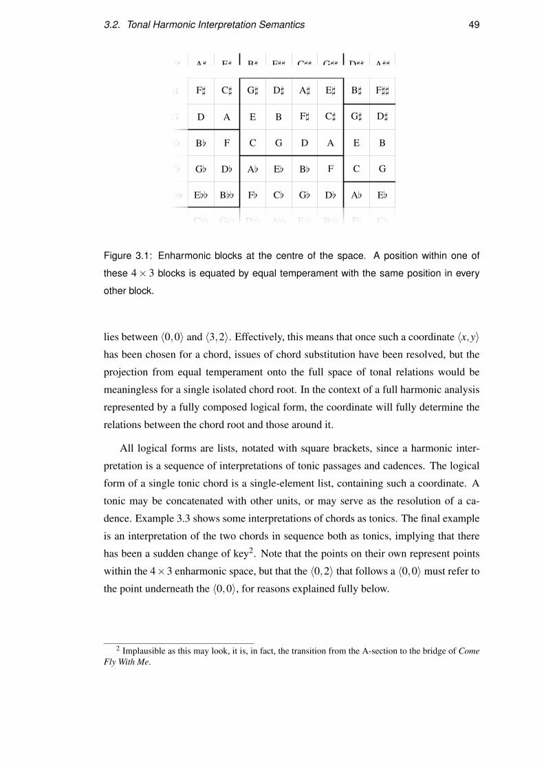
3.2. Tonal Harmonic Interpretation Semantics 49
F[[
A[[
C[
E[
G
B
D]
C[[
E[[
G[
B[
D
F]
A]
G[[
B[[
D[
F
A
C]
E]
D[[
F[
A[
C
E
G]
B]
A[[
C[
E[
G
B
D]
F]]
E[[
G[
B[
D
F]
A]
C]]
B[[
D[
F
A
C]
E]
G]]
F[
A[
C
E
G]
B]
D]]
C[
E[
G
B
D]
F]]
A]]
G[
B[
D
F]
A]
C]]
E]]
Figure 3.1: Enharmonic blocks at the centre of the space. A position within one of
these 4× 3 blocks is equated by equal temperament with the same position in every
other block.
lies between 〈0,0〉 and 〈3,2〉. Effectively, this means that once such a coordinate 〈x,y〉has been chosen for a chord, issues of chord substitution have been resolved, but the
projection from equal temperament onto the full space of tonal relations would be
meaningless for a single isolated chord root. In the context of a full harmonic analysis
represented by a fully composed logical form, the coordinate will fully determine the
relations between the chord root and those around it.
All logical forms are lists, notated with square brackets, since a harmonic inter-
pretation is a sequence of interpretations of tonic passages and cadences. The logical
form of a single tonic chord is a single-element list, containing such a coordinate. A
tonic may be concatenated with other units, or may serve as the resolution of a ca-
dence. Example 3.3 shows some interpretations of chords as tonics. The final example
is an interpretation of the two chords in sequence both as tonics, implying that there
has been a sudden change of key2. Note that the points on their own represent points
within the 4×3 enharmonic space, but that the 〈0,2〉 that follows a 〈0,0〉 must refer to
the point underneath the 〈0,0〉, for reasons explained fully below.
2 Implausible as this may look, it is, in fact, the transition from the A-section to the bridge of ComeFly With Me.

50 Chapter 3. A Grammar for Tonal Harmony
(3.3) CM7 ⇒ [〈0,0〉]
C
E
G]
G
B
D]
D
F]
A]
A
C]
E]
A[6 ⇒ [〈0,2〉]
C
E
G]
G
B
D]
D
F]
A]
A
C]
E]
C A[M7 ⇒ [〈0,0〉,〈0,2〉]
B[[
D[
F
A
F[
A[
C
E
C[
E[
G
B
3.2.3 Interpretation of Cadences
The semantics of an authentic or plagal cadence resolution is a predicate represent-
ing a movement in the tonal space. An extended cadence, of the sort described in
section 2.5.1, is interpreted as the recursive application of each movement to its reso-
lution.
Authentic (dominant) cadences are leftward steps and use the leftonto predicate.
Just as, in the linguistic logical forms, the predicate eats′ served as a notation for the
concept of eating, here the leftonto predicate stands for a direct movement in the tonal
space. Plagal (subdominant) cadences are rightward steps and use the rightonto predi-
cate. For example, a single dominant chord G7 resolving to a tonic C would receive the
logical form leftonto(〈0,0〉), whilst D7 G7 C would receive leftonto(leftonto(〈0,0〉)).A special behaviour is defined in the case of the application of a unary predicate,
like leftonto, to a list. The following reduction causes the predicate to be applied to the
first item in the list, so that the result is a list:
pred([X0,X1, ...])⇒ [pred(X0),X1, ...]

3.2. Tonal Harmonic Interpretation Semantics 51
Example 3.4 shows an interpretation of an extended cadence with two dominants
– the familiar IIm7 V7 I – derived from the logical forms of the individual chords. The
resulting tonal space path movements are shown to the right.
(3.4) Dm7 G7 C
λx. leftonto(x) λx. leftonto(x) [〈0,0〉]>
[leftonto(〈0,0〉)]>
[leftonto(leftonto(〈0,0〉))] D[
F
A
A[
C
E
E[
G
B
B[
D
F]
F
A
C]
We will see later how the syntactic types associated with logical forms constrain the
rules that may combine them in derivations. For now, derivations are shown without
the syntactic types of the constituents.
The ◦ operator denotes function composition, defined as it was for linguistic se-
mantics:
f ◦g≡ λx. f (g(x))
Here f and g may stand for a predicate like leftonto. As in the logical semantics of
language, functions can be combined using composition. The resulting function f ◦g
can then be applied to the argument x, producing the same logical form that would have
been produced by first applying g to x, then f to the result: that is, ( f ◦g)(x)≡ f (g(x)).
In the harmonic semantics, this allows us to derive a functional interpretation of a
whole cadence before seeing its resolution, as in example 3.5. It should be noted
that this particular derivation of the extended cadence is now left branching, but that
its logical form is identical to that given by the alternative derivation in the previous
example (just as in example 2.3 in chapter 2) and has a right-branching embedding.
(3.5) Dm7 G7 C
λx. leftonto(x) λx. leftonto(x) [〈0,0〉]>B
λx. leftonto(leftonto(x))>
[leftonto(leftonto(〈0,0〉))]
3.2.4 Coordination of Cadences
Logical forms representing unresolved cadences can be coordinated to represent their
sharing of the eventual resolution. This is represented by a special operator ∧. This
simply conjoins the cadence logical forms, which are always functions expecting the
resolution as their argument.
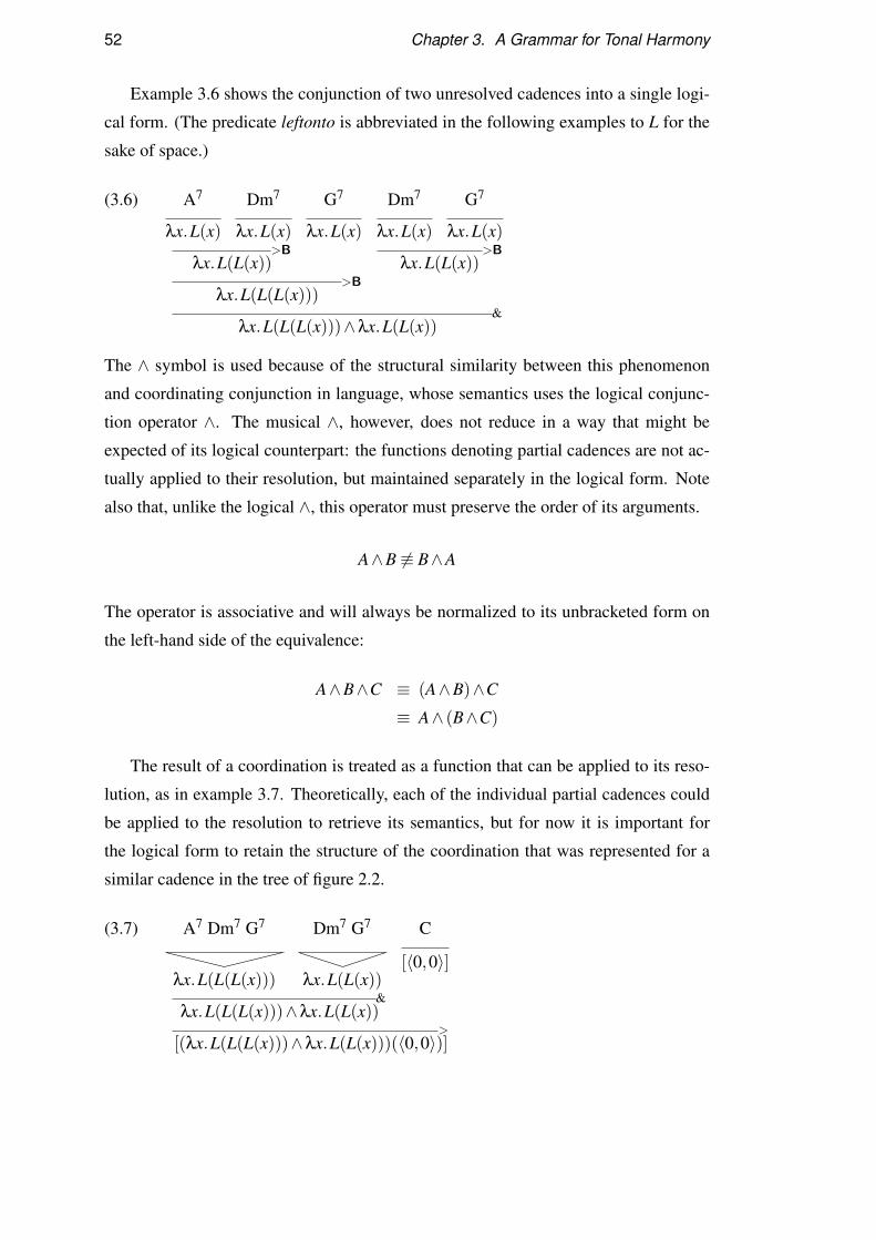
52 Chapter 3. A Grammar for Tonal Harmony
Example 3.6 shows the conjunction of two unresolved cadences into a single logi-
cal form. (The predicate leftonto is abbreviated in the following examples to L for the
sake of space.)
(3.6) A7 Dm7 G7 Dm7 G7
λx.L(x) λx.L(x) λx.L(x) λx.L(x) λx.L(x)>B >B
λx.L(L(x)) λx.L(L(x))>B
λx.L(L(L(x)))&
λx.L(L(L(x)))∧λx.L(L(x))
The ∧ symbol is used because of the structural similarity between this phenomenon
and coordinating conjunction in language, whose semantics uses the logical conjunc-
tion operator ∧. The musical ∧, however, does not reduce in a way that might be
expected of its logical counterpart: the functions denoting partial cadences are not ac-
tually applied to their resolution, but maintained separately in the logical form. Note
also that, unlike the logical ∧, this operator must preserve the order of its arguments.
A∧B 6≡ B∧A
The operator is associative and will always be normalized to its unbracketed form on
the left-hand side of the equivalence:
A∧B∧C ≡ (A∧B)∧C
≡ A∧ (B∧C)
The result of a coordination is treated as a function that can be applied to its reso-
lution, as in example 3.7. Theoretically, each of the individual partial cadences could
be applied to the resolution to retrieve its semantics, but for now it is important for
the logical form to retain the structure of the coordination that was represented for a
similar cadence in the tree of figure 2.2.
(3.7) A7 Dm7 G7 Dm7 G7 C
[〈0,0〉]λx.L(L(L(x))) λx.L(L(x))
&λx.L(L(L(x)))∧λx.L(L(x))
>[(λx.L(L(L(x)))∧λx.L(L(x)))(〈0,0〉)]
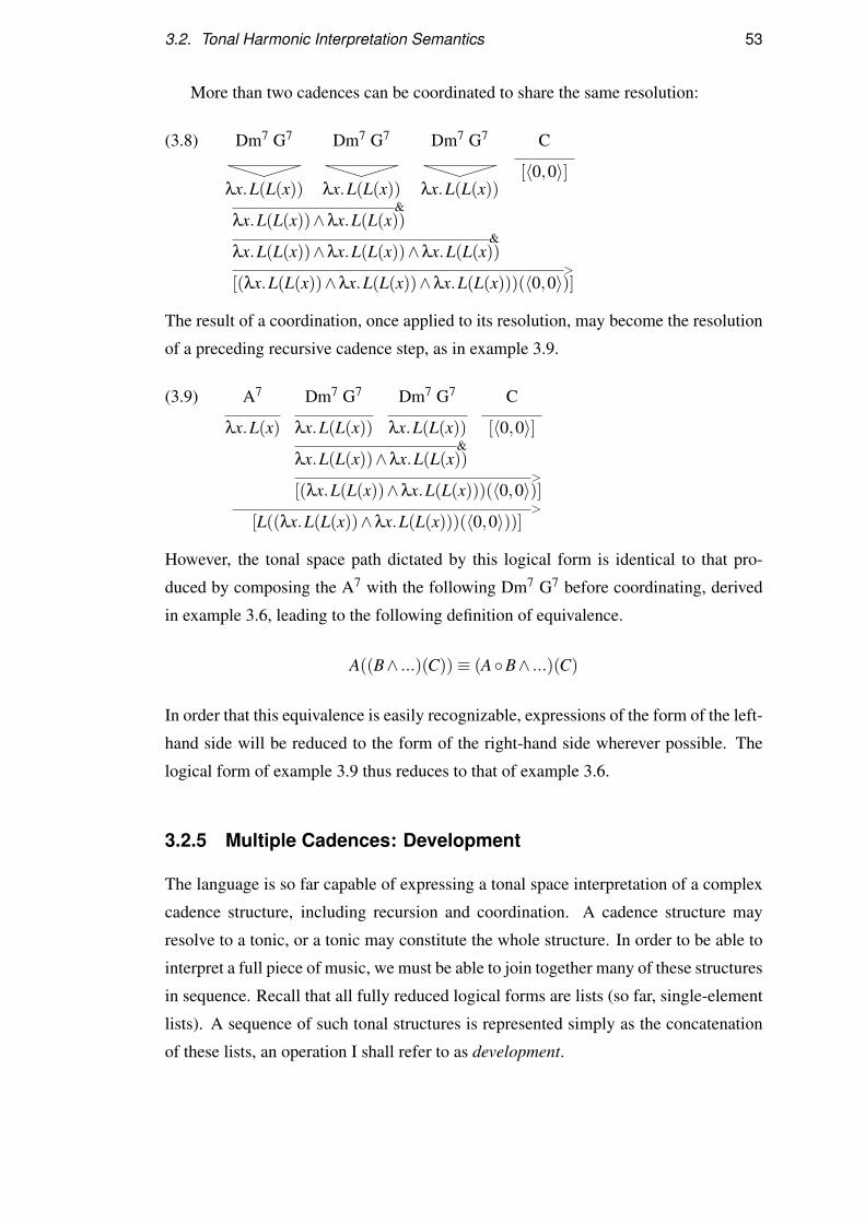
3.2. Tonal Harmonic Interpretation Semantics 53
More than two cadences can be coordinated to share the same resolution:
(3.8) Dm7 G7 Dm7 G7 Dm7 G7 C
[〈0,0〉]λx.L(L(x)) λx.L(L(x)) λx.L(L(x))
&λx.L(L(x))∧λx.L(L(x))
&λx.L(L(x))∧λx.L(L(x))∧λx.L(L(x))
>[(λx.L(L(x))∧λx.L(L(x))∧λx.L(L(x)))(〈0,0〉)]
The result of a coordination, once applied to its resolution, may become the resolution
of a preceding recursive cadence step, as in example 3.9.
(3.9) A7 Dm7 G7 Dm7 G7 C
λx.L(x) λx.L(L(x)) λx.L(L(x)) [〈0,0〉]&
λx.L(L(x))∧λx.L(L(x))>
[(λx.L(L(x))∧λx.L(L(x)))(〈0,0〉)]>
[L((λx.L(L(x))∧λx.L(L(x)))(〈0,0〉))]
However, the tonal space path dictated by this logical form is identical to that pro-
duced by composing the A7 with the following Dm7 G7 before coordinating, derived
in example 3.6, leading to the following definition of equivalence.
A((B∧ ...)(C))≡ (A◦B∧ ...)(C)
In order that this equivalence is easily recognizable, expressions of the form of the left-
hand side will be reduced to the form of the right-hand side wherever possible. The
logical form of example 3.9 thus reduces to that of example 3.6.
3.2.5 Multiple Cadences: Development
The language is so far capable of expressing a tonal space interpretation of a complex
cadence structure, including recursion and coordination. A cadence structure may
resolve to a tonic, or a tonic may constitute the whole structure. In order to be able to
interpret a full piece of music, we must be able to join together many of these structures
in sequence. Recall that all fully reduced logical forms are lists (so far, single-element
lists). A sequence of such tonal structures is represented simply as the concatenation
of these lists, an operation I shall refer to as development.

54 Chapter 3. A Grammar for Tonal Harmony
Example 3.10 shows a pair of resolved cadences being combined in this way and
example 3.11 shows a tonic passage combining with a subsequent resolved cadence.
(3.10) Dm7 G7 C G7 C
λx.leftonto(x) λx.leftonto(x) [〈0,0〉] λx.leftonto(x) [〈0,0〉)]> >
[leftonto(〈0,0〉)] [leftonto(〈0,0〉)]>
[leftonto(leftonto(〈0,0〉))]dev
[leftonto(leftonto(〈0,0〉)), leftonto(〈0,0〉)]
(3.11) C Dm7 G7 C
[〈0,0〉] λx.leftonto(x) λx.leftonto(x) [〈0,0〉]>
[leftonto(〈0,0〉)]>
[leftonto(leftonto(〈0,0〉))]dev
[〈0,0〉, leftonto(leftonto(〈0,0〉))]
3.2.6 Colouration: Empty Semantics
Some brief harmonic excursions add colouration to a piece, but contribute little to the
functional structure of the harmony. It is convenient to ignore these for the purposes
of harmonic analysis. A typical example is the sequence I IV I, often played during
long passages of a I chord. This could be analysed as a form of plagal cadence and in
a fine-grained analysis this might be appropriate. Another example is passing chords,
which resemble diminished seventh chords or diminished triads, but have no harmonic
function.
Such chords can be ignored by assigning them a logical form that is the identity
function: λx.x. Example 3.12 shows this in action on a I IV I sequence.
(3.12) C F C
λx.x λx.x [〈0,0〉]>
[〈0,0〉]>
[〈0,0〉]

3.2. Tonal Harmonic Interpretation Semantics 55
3.2.7 Extracting the Tonal Space Path
3.2.7.1 Path Constraints
A logical form can be seen as denoting a set of constraints on the path through the
tonal space traced by the roots of the chords. The full path can be inferred from a fully
formed logical form, given an arbitrary starting point. Since the tonal space is a space
of tonal relations between chords, absolute position in the space is meaningless. The
arbitrary choice of the starting point of a path sets a reference point to begin the series
of tonal relations.
Let us first examine the constraints encoded in the various types of predicate. The
movement made by leftonto(p) begins one step in the grid to the right of the first
point of the path p. Given an unambiguous resolution to a point (x,y), the whole path
leftonto(leftonto((x,y))) is also unambiguous. Two cadences that share a resolution
through coordination are constrained to end at the same point, since their paths are
constrained relative to their shared resolution. There is no obvious constraint between
items in a list, which are either tonics or resolved cadences. They are, therefore, linked
by the closest tonal relation (the smallest possible Manhattan distance) that satisfies all
other constraints.
For example, consider the two logical forms shown in figure 3.2 with their tonal
space paths. The start of the second item in logical form (a) is dependent, ultimately,
on the cadence resolution 〈0,0〉. This point, as distinct from (0,0), is ambiguous:
we can choose for it any of the infinite points that lie at (0,0) within their enhar-
monic block. Taking the start of the path to be at the central (0,0), we choose the
same point for the end of the second item, since it puts the start of the second item,
leftonto(leftonto(〈0,0〉)), as close as possible to (0,0). A choice of (−4,1) (dashed)
for the final resolution would also have been permitted by other constraints, but would
have resulted in a larger jump between the two path fragments.
In logical form (b), on the other hand, the second item begins at a point further
from its ending, since it includes three left steps. In this case we must choose (−1,1)
as the start point for the second item by putting its resolution 〈0,0〉 at (−4,1).
3.2.7.2 The Algorithm
Algorithm 1 uses the information encoded in a logical form to produce the correspond-
ing interpretation as a path through the tonal space. As well as demonstrating that any
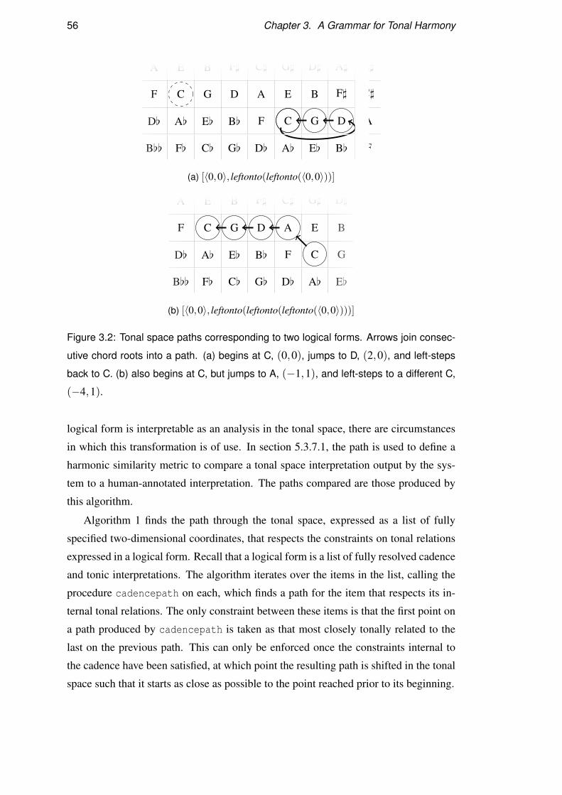
56 Chapter 3. A Grammar for Tonal Harmony
B[[
D[
F
A
F[
A[
C
E
C[
E[
G
B
G[
B[
D
F]
D[
F
A
C]
A[
C
E
G]
E[
G
B
D]
B[
D
F]
A]
F
A
C]
E]
(a) [〈0,0〉, leftonto(leftonto(〈0,0〉))]
B[[
D[
F
A
F[
A[
C
E
C[
E[
G
B
G[
B[
D
F]
D[
F
A
C]
A[
C
E
G]
E[
G
B
D]
(b) [〈0,0〉, leftonto(leftonto(leftonto(〈0,0〉)))]
Figure 3.2: Tonal space paths corresponding to two logical forms. Arrows join consec-
utive chord roots into a path. (a) begins at C, (0,0), jumps to D, (2,0), and left-steps
back to C. (b) also begins at C, but jumps to A, (−1,1), and left-steps to a different C,
(−4,1).
logical form is interpretable as an analysis in the tonal space, there are circumstances
in which this transformation is of use. In section 5.3.7.1, the path is used to define a
harmonic similarity metric to compare a tonal space interpretation output by the sys-
tem to a human-annotated interpretation. The paths compared are those produced by
this algorithm.
Algorithm 1 finds the path through the tonal space, expressed as a list of fully
specified two-dimensional coordinates, that respects the constraints on tonal relations
expressed in a logical form. Recall that a logical form is a list of fully resolved cadence
and tonic interpretations. The algorithm iterates over the items in the list, calling the
procedure cadencepath on each, which finds a path for the item that respects its in-
ternal tonal relations. The only constraint between these items is that the first point on
a path produced by cadencepath is taken as that most closely tonally related to the
last on the previous path. This can only be enforced once the constraints internal to
the cadence have been satisfied, at which point the resulting path is shifted in the tonal
space such that it starts as close as possible to the point reached prior to its beginning.

3.2. Tonal Harmonic Interpretation Semantics 57
Algorithm 1: path(lf) – output tonal space path for a logical form
1 endpoint← (0,0)
2 foreach cadence in lf do3 points← cadencepath(cadence)
4 shift points to make closest connection with endpoint
5 print(points)
6 endpoint← last(points)
Procedure cadencepath(cad) – tonal space path for a cadence (see algorithm 1)
1 path← [root(cad)]
2 foreach predicate applied to root of cad, innermost first do3 if predicate = rightonto then prepend(path,path0 +(−1,0))
4 else if predicate = leftonto then prepend(path,path0 +(1,0))
5 else if predicate = (C0 & . . . & Cn) then6 resolution← path0
7 foreach Ci←Cn, . . . ,C0 do8 cadpath← cadencepath(Ci(resolution))
9 remove last point from cadpath
10 prepend(path,cadpath)
11 return path
The procedure cadencepath produces a path from the logical form of a single
cadence. It begins by taking the root of the predicate structure – that is, the tonic to
which it eventually resolves – to be that closest to (0,0), relative to which the rest of
the path fragment will be built. The algorithm then works its way outwards through
the predicate applications, adding points to the path. Predicates leftonto and rightonto
take a single argument and add a point to the start of the path respectively one step to
the right and left of the current first point. A coordination structure contains several
structures representing unresolved cadences. They all must resolve to the argument to
which the coordination is applied. Therefore, each cadence in turn is transformed into a
path by a recursive call to cadencepath, taking the resolution to be the point currently
at the start of the path. The resulting path fragment for each cadence is prepended to
the path (removing the point that was treated as the resolution, so that it is not repeated
at the end of each cadence).
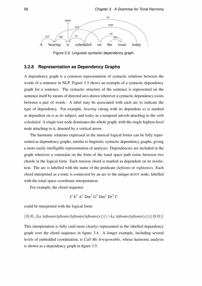
58 Chapter 3. A Grammar for Tonal Harmony
A hearing is scheduled on the issue today .
PRED
ATT
ATT
SBJ
PU
VC
TMP
PCATT
Figure 3.3: Linguistic syntactic dependency graph.
3.2.8 Representation as Dependency Graphs
A dependency graph is a common representation of syntactic relations between the
words of a sentence in NLP. Figure 3.3 shows an example of a syntactic dependency
graph for a sentence. The syntactic structure of the sentence is represented on the
sentence itself by means of directed arcs drawn wherever a syntactic dependency exists
between a pair of words. A label may be associated with each arc to indicate the
type of dependency. For example, hearing (along with its dependent a) is marked
as dependent on is as its subject, and today as a temporal adverb attaching to the verb
scheduled. A single root node dominates the whole graph, with the single highest-level
node attaching to it, denoted by a vertical arrow.
The harmonic relations expressed in the musical logical forms can be fully repre-
sented as dependency graphs, similar to linguistic syntactic dependency graphs, giving
a more easily intelligible representation of analyses. Dependencies are included in the
graph wherever a constraint on the form of the tonal space path exists between two
chords in the logical form. Each tension chord is marked as dependent on its resolu-
tion. The arc is labelled with the name of the predicate (leftonto or rightonto). Each
chord interpreted as a tonic is connected by an arc to the unique ROOT node, labelled
with the tonal space coordinate interpretation.
For example, the chord sequence
C E7 A7 Dm7 G7 Dm7 D[7 C
could be interpreted with the logical form:
[〈0,0〉,(λx. leftonto(leftonto(leftonto(leftonto(x))))∧λx. leftonto(leftonto(x)))(〈0,0〉)]
This interpretation is fully (and more clearly) represented as the labelled dependency
graph over the chord sequence in figure 3.4. A longer example, including several
levels of embedded coordination, is Call Me Irresponsible, whose harmonic analysis
is shown as a dependency graph in figure 3.5.
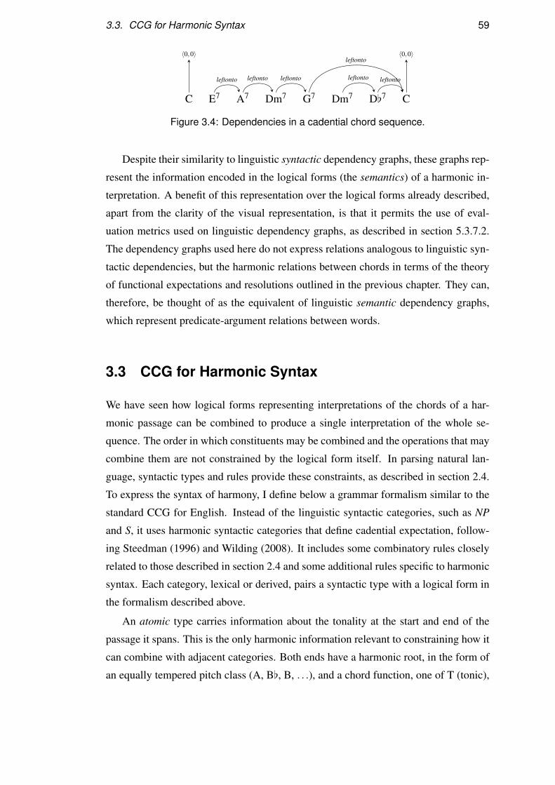
3.3. CCG for Harmonic Syntax 59
C E7 A7 Dm7 G7 Dm7 D[7 C
〈0,0〉 〈0,0〉
leftonto leftonto leftonto
leftonto
leftonto leftonto
Figure 3.4: Dependencies in a cadential chord sequence.
Despite their similarity to linguistic syntactic dependency graphs, these graphs rep-
resent the information encoded in the logical forms (the semantics) of a harmonic in-
terpretation. A benefit of this representation over the logical forms already described,
apart from the clarity of the visual representation, is that it permits the use of eval-
uation metrics used on linguistic dependency graphs, as described in section 5.3.7.2.
The dependency graphs used here do not express relations analogous to linguistic syn-
tactic dependencies, but the harmonic relations between chords in terms of the theory
of functional expectations and resolutions outlined in the previous chapter. They can,
therefore, be thought of as the equivalent of linguistic semantic dependency graphs,
which represent predicate-argument relations between words.
3.3 CCG for Harmonic Syntax
We have seen how logical forms representing interpretations of the chords of a har-
monic passage can be combined to produce a single interpretation of the whole se-
quence. The order in which constituents may be combined and the operations that may
combine them are not constrained by the logical form itself. In parsing natural lan-
guage, syntactic types and rules provide these constraints, as described in section 2.4.
To express the syntax of harmony, I define below a grammar formalism similar to the
standard CCG for English. Instead of the linguistic syntactic categories, such as NP
and S, it uses harmonic syntactic categories that define cadential expectation, follow-
ing Steedman (1996) and Wilding (2008). It includes some combinatory rules closely
related to those described in section 2.4 and some additional rules specific to harmonic
syntax. Each category, lexical or derived, pairs a syntactic type with a logical form in
the formalism described above.
An atomic type carries information about the tonality at the start and end of the
passage it spans. This is the only harmonic information relevant to constraining how it
can combine with adjacent categories. Both ends have a harmonic root, in the form of
an equally tempered pitch class (A, B[, B, . . .), and a chord function, one of T (tonic),
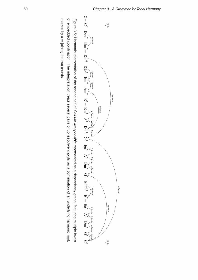
60 Chapter 3. A Grammar for Tonal Harmony
C=
C6
D[◦
7D
m7=
Dm
6D]◦
7E
m7
Am
7E
7=E
m7
A7
Dm
7G
7E
ø7
A7
Dm
7G
7B
sus4,7E
7=E
ø7
A7
Dm
7G
7C
6
〈0,0〉
leftontoleftonto
leftontoleftonto
leftonto
leftonto
leftonto
leftontoleftonto
leftontoleftonto
leftontoleftonto
leftontoleftonto
leftonto
leftonto
leftonto 〈0,0〉
Figure3.5:
Harm
onicinterpretation
ofthesecond
halfofCallM
eIrresponsible
representedas
adependency
graph,featuringm
ultiplelevels
ofem
beddedcoordination.
Theinterpretation
treatsseveralpairs
ofconsecutive
chordsas
acontinuation
ofan
underlyingharm
onicroot,
marked
bya=
joiningthe
two
chords.

3.3. CCG for Harmonic Syntax 61
D (dominant) and S (subdominant), written as a superscript. For example, a passage
starting on a tonic C and ending on a tonic A[ would have syntactic type CT –A[T .
For brevity, where the start and end parts of an atomic type are the same, just one is
written: CT –CT is abbreviated to CT . Such a type is associated with a single tonic
chord.
A forward-facing slash type X/Y gives the starting tonality Y expected for the
category to its right (its argument) and the starting tonality X that will be used for the
result of applying it to such an argument. Such a type is used in the interpretation of
a dominant chord. We are now able to associate syntactic types of this sort with the
logical forms of section 3.2 in order to constrain the ways adjacent constituents can be
combined, according to the definitions of the combinatorial rules, given in full below.
Example 3.13 adds syntactic types to example 3.11. As is conventional, the syntactic
type is given first, separated from the logical form by a colon.
(3.13) C Dm7 G7 C
CT : [〈0,0〉] DD/GD|T GD/CD|T CT : [〈0,0〉]: λx.leftonto(x) : λx.leftonto(x)
>
GD–CT : [leftonto(〈0,0〉)]>
DD–CT : [leftonto(leftonto(〈0,0〉))]dev
CT : [〈0,0〉, leftonto(leftonto(〈0,0〉))]
The categories assumed by Dm7 and G7 are identical, relative to the roots of the chord
labels, and are specified by a single schema ID/IV D|T : λx. leftonto(x) in the lexicon,
using Roman numerals to express pitch relative to the chord root. A primitive domi-
nant chord could be interpreted with the syntactic type schema ID/IV T , reflecting the
expectation of a resolution down a perfect fifth to follow. Extended cadences, such as
the one in example 3.13, are handled syntactically by allowing the dominant category
to take as its resolution either a tonic or another dominant by using the type ID/IV D|T .
The combinatorial rule that performs function composition (as in example 3.5)
performs the appropriate manipulation of the syntactic categories:
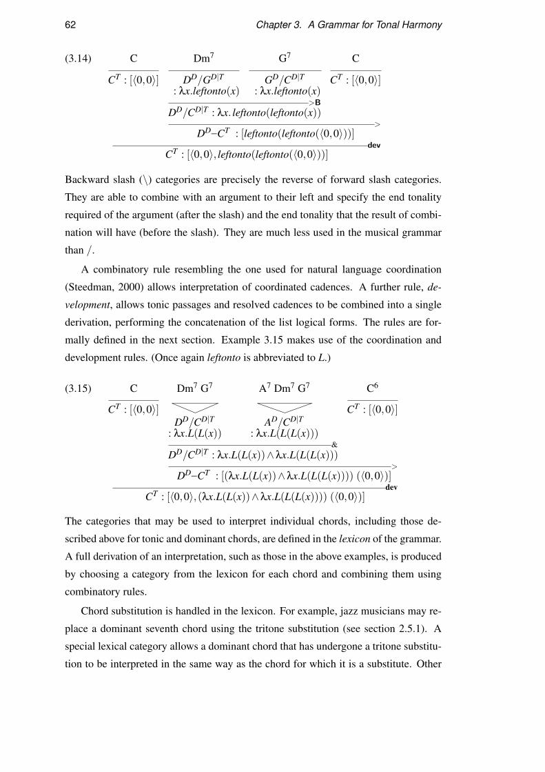
62 Chapter 3. A Grammar for Tonal Harmony
(3.14) C Dm7 G7 C
CT : [〈0,0〉] DD/GD|T GD/CD|T CT : [〈0,0〉]: λx.leftonto(x) : λx.leftonto(x)
>B
DD/CD|T : λx. leftonto(leftonto(x))>
DD–CT : [leftonto(leftonto(〈0,0〉))]dev
CT : [〈0,0〉, leftonto(leftonto(〈0,0〉))]
Backward slash (\) categories are precisely the reverse of forward slash categories.
They are able to combine with an argument to their left and specify the end tonality
required of the argument (after the slash) and the end tonality that the result of combi-
nation will have (before the slash). They are much less used in the musical grammar
than /.
A combinatory rule resembling the one used for natural language coordination
(Steedman, 2000) allows interpretation of coordinated cadences. A further rule, de-
velopment, allows tonic passages and resolved cadences to be combined into a single
derivation, performing the concatenation of the list logical forms. The rules are for-
mally defined in the next section. Example 3.15 makes use of the coordination and
development rules. (Once again leftonto is abbreviated to L.)
(3.15) C Dm7 G7 A7 Dm7 G7 C6
CT : [〈0,0〉] CT : [〈0,0〉]DD/CD|T AD/CD|T
: λx.L(L(x)) : λx.L(L(L(x)))&
DD/CD|T : λx.L(L(x))∧λx.L(L(L(x)))>
DD–CT : [(λx.L(L(x))∧λx.L(L(L(x)))) (〈0,0〉)]dev
CT : [〈0,0〉,(λx.L(L(x))∧λx.L(L(L(x)))) (〈0,0〉)]
The categories that may be used to interpret individual chords, including those de-
scribed above for tonic and dominant chords, are defined in the lexicon of the grammar.
A full derivation of an interpretation, such as those in the above examples, is produced
by choosing a category from the lexicon for each chord and combining them using
combinatory rules.
Chord substitution is handled in the lexicon. For example, jazz musicians may re-
place a dominant seventh chord using the tritone substitution (see section 2.5.1). A
special lexical category allows a dominant chord that has undergone a tritone substitu-
tion to be interpreted in the same way as the chord for which it is a substitute. Other
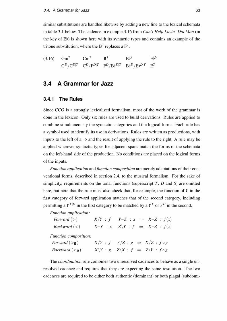
3.4. A Grammar for Jazz 63
similar substitutions are handled likewise by adding a new line to the lexical schemata
in table 3.1 below. The cadence in example 3.16 from Can’t Help Lovin’ Dat Man (in
the key of E[) is shown here with its syntactic types and contains an example of the
tritone substitution, where the B7 replaces a F7.
(3.16) Gm7
GD/CD|TCm7
CD/FD|TB7
FD/B[D|TB[7
B[D/E[D|TE[6
ET
3.4 A Grammar for Jazz
3.4.1 The Rules
Since CCG is a strongly lexicalized formalism, most of the work of the grammar is
done in the lexicon. Only six rules are used to build derivations. Rules are applied to
combine simultaneously the syntactic categories and the logical forms. Each rule has
a symbol used to identify its use in derivations. Rules are written as productions, with
inputs to the left of a⇒ and the result of applying the rule to the right. A rule may be
applied wherever syntactic types for adjacent spans match the forms of the schemata
on the left-hand side of the production. No conditions are placed on the logical forms
of the inputs.
Function application and function composition are merely adaptations of their con-
ventional forms, described in section 2.4, to the musical formalism. For the sake of
simplicity, requirements on the tonal functions (superscript T , D and S) are omitted
here, but note that the rule must also check that, for example, the function of Y in the
first category of forward application matches that of the second category, including
permitting a Y T |D in the first category to be matched by a Y T or Y D in the second.
Function application:Forward (>) X/Y : f Y –Z : x ⇒ X–Z : f (x)
Backward (<) X–Y : x Z\Y : f ⇒ X–Z : f (x)
Function composition:Forward (>B) X/Y : f Y/Z : g ⇒ X/Z : f ◦g
Backward (<B) X\Y : g Z\X : f ⇒ Z\Y : f ◦g
The coordination rule combines two unresolved cadences to behave as a single un-
resolved cadence and requires that they are expecting the same resolution. The two
cadences are required to be either both authentic (dominant) or both plagal (subdomi-

64 Chapter 3. A Grammar for Tonal Harmony
nant). The logical form of the result is treated as a function that will be applied to the
resolution.
Coordination:
(&) XF/Y : f ZF/Y : g ⇒ XF/Y : f ∧g where F ∈ {D,S}
The trivial development rule joins together fully resolved passages. It requires its
inputs to be atomic categories and not slash categories, which need to be combined
with something by function application before they can be considered resolved. Syn-
tactic constraints and the composition of the lexicon ensure that such an atomic cate-
gory will always have a list logical form, so this rule can simply concatenate the two
lists.
Development:
(dev) V –W : l0 X–Y : l1 ⇒ V –Y : l0⊕ l1
This is a permissive rule: it permits any two consecutive passages interpreted in-
dividually as harmonically stable to be conjoined, regardless of key. Modulation (key
change) can occur freely in music at any time. We, therefore, do not use the grammar
to put any restrictions on what sorts of modulation to permit. Whilst some modula-
tions are more common than others, such preferences are better captured by statistical
models, such as those introduced in chapter 5, than by syntactic constraints.
In addition to the lexical schemata given in the next section, the lexicon is expanded
by the application of two unary rules. These provide categories to handle the repeti-
tion of chords without a change in harmonic function. This occurs sometimes simply
because of notational conventions – a chord will often be repeated at the beginning of
a new line or section, even if it is really just a continuation of the previous chord – and
sometimes because there is a change in the chord at a level which is not reflected in
the analysis. The former case could be handled simply by preprocessing the input to
remove repeated chords, but the latter cannot be dismissed as easily.
For example, say a tonic chord CM7 is followed by a chord on the same root with
a different chord type C6. The change in chord type is important for performers, but
is irrelevant to the analysis. A chord might also be followed by another on a different
root which behaves as a substitute for the first. In this case too, the chords should
be combined early in the analysis into a single unit. For example, McCoy Tyner’s
Contemplation begins on a Cm7(11) chord, establishing the tonic of the piece, for the
first two lines. The third line is on an A[M7 chord, behaving as a substitute for the Cm
chord (really nothing more than an inversion). This can be interpreted as a substitution

3.4. A Grammar for Jazz 65
using a special lexical category (Ton-bVI, see the lexicon in the next section). The two
chords are then treated as a single tonic passage.
Dominant and subdominant chords too can be prolonged in this manner, similarly
permitting movement between different substitutions for the same chord. The follow-
ing two rules produce lexical schemata that can be applied to the first of such a pair of
chords in place of the schema that it would have had on its own. The resulting lexical
schemata will be referred to using a mnemonic distinguished from that of the original
schema by the addition of ‘-rep’.
Tonic repetition:
(TRep) XT : f ⇒ XT/XT : λx.x
Cadence repetition:
(CRep) XF/Y : f ⇒ XF/XF : λx.x where F ∈ {D,S}
The tonic passage of Contemplation can now be interpreted as shown in exam-
ple 3.17, using the Ton-bVI schema and Ton-rep, which is produced from the Ton
schema (see next section) using the tonic repetition rule.
(3.17) Cm7(11) A[7
CT/CT : λx.x CT : [〈0,0〉]>
CT : [〈0,0〉]
The unary rules of tonic repetition and cadence repetition are restricted to the role of
expanding the lexicon and cannot be applied at any other point in a derivation3. For
example, the category resulting from the derivation in example 3.17 cannot be used as
input to the tonic repetition rule to produce the category CT/CT : λx.x.
3.4.2 The Lexicon
We are now able to define in full the lexicon of a grammar of jazz chord sequences,
shown in table 3.1. Each entry is a lexical schema and has a mnemonic label to serve
as an identifier, a surface chord class, a syntactic type and a logical form. The surface
chord class generalizes over chord roots X and the syntactic type is given relative to the
root of the surface chord symbol, using Roman numeral notation. For example, if the
first entry, Ton, were assigned to a chord G, the syntactic type of the category would be
GT . During parsing, a lexical schema may be specialized to a particular root pitch to
3 A similar restriction is typically put on the type raising rule in CCG for natural language.
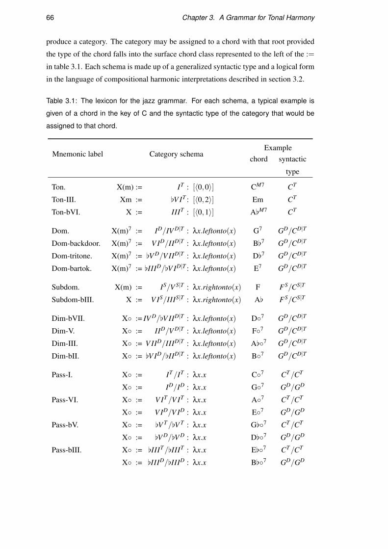
66 Chapter 3. A Grammar for Tonal Harmony
produce a category. The category may be assigned to a chord with that root provided
the type of the chord falls into the surface chord class represented to the left of the :=
in table 3.1. Each schema is made up of a generalized syntactic type and a logical form
in the language of compositional harmonic interpretations described in section 3.2.
Table 3.1: The lexicon for the jazz grammar. For each schema, a typical example is
given of a chord in the key of C and the syntactic type of the category that would be
assigned to that chord.
Mnemonic label Category schemaExample
chord syntactic
type
Ton. X(m) := IT : [〈0,0〉] CM7 CT
Ton-III. Xm := [V IT : [〈0,2〉] Em CT
Ton-bVI. X := IIIT : [〈0,1〉] A[M7 CT
Dom. X(m)7 := ID/IV D|T : λx.leftonto(x) G7 GD/CD|T
Dom-backdoor. X(m)7 := V ID/IID|T : λx.leftonto(x) B[7 GD/CD|T
Dom-tritone. X(m)7 := [V D/V IID|T : λx.leftonto(x) D[7 GD/CD|T
Dom-bartok. X(m)7 := [IIID/[V ID|T : λx.leftonto(x) E7 GD/CD|T
Subdom. X(m) := IS/V S|T : λx.rightonto(x) F FS/CS|T
Subdom-bIII. X := V IS/IIIS|T : λx.rightonto(x) A[ FS/CS|T
Dim-bVII. X◦ := IV D/[V IID|T : λx.leftonto(x) D◦7 GD/CD|T
Dim-V. X◦ := IID/V D|T : λx.leftonto(x) F◦7 GD/CD|T
Dim-III. X◦ := V IID/IIID|T : λx.leftonto(x) A[◦7 GD/CD|T
Dim-bII. X◦ := [V ID/[IID|T : λx.leftonto(x) B◦7 GD/CD|T
Pass-I. X◦ := IT/IT : λx.x C◦7 CT/CT
X◦ := ID/ID : λx.x G◦7 GD/GD
Pass-VI. X◦ := V IT/V IT : λx.x A◦7 CT/CT
X◦ := V ID/V ID : λx.x E◦7 GD/GD
Pass-bV. X◦ := [V T/[V T : λx.x G[◦7 CT/CT
X◦ := [V D/[V D : λx.x D[◦7 GD/GD
Pass-bIII. X◦ := [IIIT/[IIIT : λx.x E[◦7 CT/CT
X◦ := [IIID/[IIID : λx.x B[◦7 GD/GD
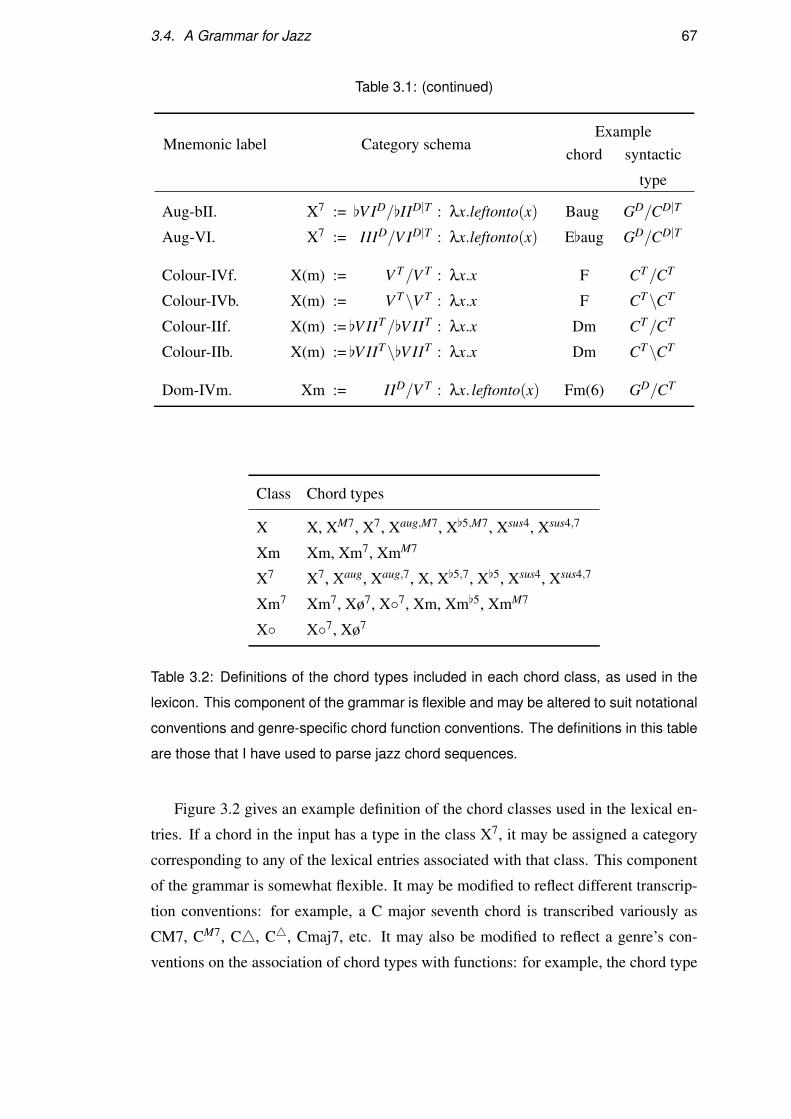
3.4. A Grammar for Jazz 67
Table 3.1: (continued)
Mnemonic label Category schemaExample
chord syntactic
type
Aug-bII. X7 := [V ID/[IID|T : λx.leftonto(x) Baug GD/CD|T
Aug-VI. X7 := IIID/V ID|T : λx.leftonto(x) E[aug GD/CD|T
Colour-IVf. X(m) := V T/V T : λx.x F CT/CT
Colour-IVb. X(m) := V T\V T : λx.x F CT\CT
Colour-IIf. X(m) := [V IIT/[V IIT : λx.x Dm CT/CT
Colour-IIb. X(m) := [V IIT\[V IIT : λx.x Dm CT\CT
Dom-IVm. Xm := IID/V T : λx. leftonto(x) Fm(6) GD/CT
Class Chord types
X X, XM7, X7, Xaug,M7, X[5,M7, Xsus4, Xsus4,7
Xm Xm, Xm7, XmM7
X7 X7, Xaug, Xaug,7, X, X[5,7, X[5, Xsus4, Xsus4,7
Xm7 Xm7, Xø7, X◦7, Xm, Xm[5, XmM7
X◦ X◦7, Xø7
Table 3.2: Definitions of the chord types included in each chord class, as used in the
lexicon. This component of the grammar is flexible and may be altered to suit notational
conventions and genre-specific chord function conventions. The definitions in this table
are those that I have used to parse jazz chord sequences.
Figure 3.2 gives an example definition of the chord classes used in the lexical en-
tries. If a chord in the input has a type in the class X7, it may be assigned a category
corresponding to any of the lexical entries associated with that class. This component
of the grammar is somewhat flexible. It may be modified to reflect different transcrip-
tion conventions: for example, a C major seventh chord is transcribed variously as
CM7, CM7, C4, C4, Cmaj7, etc. It may also be modified to reflect a genre’s con-
ventions on the association of chord types with functions: for example, the chord type
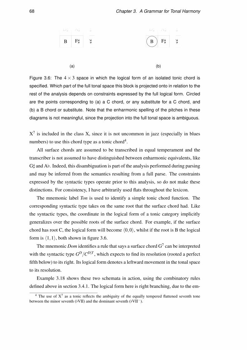
68 Chapter 3. A Grammar for Tonal Harmony
C
E
G]
G
B
D]
D
F]
A]
A
C]
E]
(a)
C
E
G]
G
B
D]
D
F]
A]
A
C]
E]
(b)
Figure 3.6: The 4× 3 space in which the logical form of an isolated tonic chord is
specified. Which part of the full tonal space this block is projected onto in relation to the
rest of the analysis depends on constraints expressed by the full logical form. Circled
are the points corresponding to (a) a C chord, or any substitute for a C chord, and
(b) a B chord or substitute. Note that the enharmonic spelling of the pitches in these
diagrams is not meaningful, since the projection into the full tonal space is ambiguous.
X7 is included in the class X, since it is not uncommon in jazz (especially in blues
numbers) to use this chord type as a tonic chord4.
All surface chords are assumed to be transcribed in equal temperament and the
transcriber is not assumed to have distinguished between enharmonic equivalents, like
G] and A[. Indeed, this disambiguation is part of the analysis performed during parsing
and may be inferred from the semantics resulting from a full parse. The constraints
expressed by the syntactic types operate prior to this analysis, so do not make these
distinctions. For consistency, I have arbitrarily used flats throughout the lexicon.
The mnemonic label Ton is used to identify a simple tonic chord function. The
corresponding syntactic type takes on the same root that the surface chord had. Like
the syntactic types, the coordinate in the logical form of a tonic category implicitly
generalizes over the possible roots of the surface chord. For example, if the surface
chord has root C, the logical form will become 〈0,0〉, whilst if the root is B the logical
form is 〈1,1〉, both shown in figure 3.6.
The mnemonic Dom identifies a rule that says a surface chord G7 can be interpreted
with the syntactic type GD/CD|T , which expects to find its resolution (rooted a perfect
fifth below) to its right. Its logical form denotes a leftward movement in the tonal space
to its resolution.
Example 3.18 shows these two schemata in action, using the combinatory rules
defined above in section 3.4.1. The logical form here is right branching, due to the em-
4 The use of X7 as a tonic reflects the ambiguity of the equally tempered flattened seventh tonebetween the minor seventh ([VII) and the dominant seventh ([VII−).
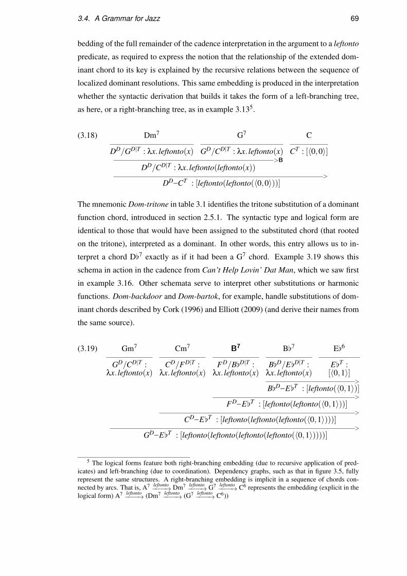
3.4. A Grammar for Jazz 69
bedding of the full remainder of the cadence interpretation in the argument to a leftonto
predicate, as required to express the notion that the relationship of the extended dom-
inant chord to its key is explained by the recursive relations between the sequence of
localized dominant resolutions. This same embedding is produced in the interpretation
whether the syntactic derivation that builds it takes the form of a left-branching tree,
as here, or a right-branching tree, as in example 3.135.
(3.18) Dm7 G7 C
DD/GD|T : λx. leftonto(x) GD/CD|T : λx. leftonto(x) CT : [〈0,0〉]>B
DD/CD|T : λx. leftonto(leftonto(x))>
DD–CT : [leftonto(leftonto(〈0,0〉))]
The mnemonic Dom-tritone in table 3.1 identifies the tritone substitution of a dominant
function chord, introduced in section 2.5.1. The syntactic type and logical form are
identical to those that would have been assigned to the substituted chord (that rooted
on the tritone), interpreted as a dominant. In other words, this entry allows us to in-
terpret a chord D[7 exactly as if it had been a G7 chord. Example 3.19 shows this
schema in action in the cadence from Can’t Help Lovin’ Dat Man, which we saw first
in example 3.16. Other schemata serve to interpret other substitutions or harmonic
functions. Dom-backdoor and Dom-bartok, for example, handle substitutions of dom-
inant chords described by Cork (1996) and Elliott (2009) (and derive their names from
the same source).
(3.19) Gm7 Cm7 B7 B[7 E[6
GD/CD|T : CD/FD|T : FD/B[D|T : B[D/E[D|T : E[T :λx. leftonto(x) λx. leftonto(x) λx. leftonto(x) λx. leftonto(x) [〈0,1〉]
>
B[D–E[T : [leftonto(〈0,1〉)]>
FD–E[T : [leftonto(leftonto(〈0,1〉))]>
CD–E[T : [leftonto(leftonto(leftonto(〈0,1〉)))]>
GD–E[T : [leftonto(leftonto(leftonto(leftonto(〈0,1〉))))]
5 The logical forms feature both right-branching embedding (due to recursive application of pred-icates) and left-branching (due to coordination). Dependency graphs, such as that in figure 3.5, fullyrepresent the same structures. A right-branching embedding is implicit in a sequence of chords con-nected by arcs. That is, A7 leftonto−−−−→ Dm7 leftonto−−−−→ G7 leftonto−−−−→ C6 represents the embedding (explicit in thelogical form) A7 leftonto−−−−→ (Dm7 leftonto−−−−→ (G7 leftonto−−−−→ C6))

70 Chapter 3. A Grammar for Tonal Harmony
T RG
T RG
T RG
T RG
G
T RG
Em
T RG
DRG
SRG
C
DRG
D
T RG
G
DRG
T RD
DRD
SRD
G
DRD
A
T RD
D
Figure 3.7: Harmonic analysis of the first two bars of Bach’s Ermuntre Dich, mein
schwacher Geist, simplified from that of Rohrmeier (2011, figure 3).
3.5 Key Structure
Neither the formal language of harmonic interpretation nor the syntactic grammar pre-
sented above provides a means of interpreting hierarchical relations between resolved
cadences or tonic passages. Each cadence is individually interpreted as a structure
made up of tension-resolution relationships and these structures are presented in se-
quence as an interpretation of an entire piece. Modulation and tonicization (a form of
short-term modulation) are permitted, since the grammar does not constrain the struc-
tures to remain in the same key throughout. However, this analysis overlooks one
aspect of the structure of harmony – the hierarchical relationships between these local
structures.
Rohrmeier (2011) captures these relationships in his harmonic grammar. He per-
mits a full recursive cadence structure to serve not only as an element in the global
sequence of phrases – rather like the top-level list structure of the logical forms pre-
sented here – but also as a functional region within another cadence structure. This
allows an entire local key structure to be interpreted, for example, as functioning as a
dominant chord with respect to a tonic at a higher level.
Consider the analysis of the opening of Bach’s Ermuntre Dich, mein schwacher
Geist given by Rohrmeier (2011, figure 3), presented in a simplified form in figure 3.7.
The non-terminals T R and DR represent tonic and dominant functional regions and

3.5. Key Structure 71
carry a feature denoting their key, written here as a subscript. The first two chords are
interpreted as a tonic passage in G major. The following chords, C D G, are treated as
a subdominant-dominant-tonic progression, still in G major. The jazz grammar of this
chapter does not include rules to handle this progression, reflecting a difference in the
intended domains of the two grammars. Where these five chords are combined, we see
the first example of a level of structural interpretation not analysed in the present the-
sis. The tree6 maintains the hierarchical structure of the combination of tonic regions
T RG into higher-level T RGs: the G and Em first, then this subtree with the tree of the
following three chords.
The final three chords, G A D, are again interpreted as a subdominant-dominant-
tonic progression, but this time in the key of D major. A unary expansion allows
this whole T RD tonic region to be treated as a dominant region DRG in a higher-level
structure. Rohrmeier’s grammar includes a rule T R→ T R DR, allowing a tonic region
to be followed by a dominant region. This leads to the full interpretation, in which
the initial tonic region is combined with the cadence in D major by the same rule that
would allow it to be followed by a single D major chord.
This example includes two types of structure ignored by the present thesis: the
hierarchical structure of tonic regions (as in the combination of T RGs on the left side)
and the analysis of whole tonic regions as fulfilling harmonic function in another key
at a higher level (as in the DRG → T RD expansion). The first extension required to
permit the present grammar to produce these analyses would be to the formal language
of section 3.2. Syntactic rules or lexical entries could then be added to derive the
structures. The hierarchical structure of cadences could be interpreted, for example,
by modification of the development rule. The interpretation of resolved passages as
having a function in the key of an adjacent passage could, at least in some cases, be
lexicalized using the music theoretic concept of a pivot chord – a chord at the junction
of two passages that has one function in the first and another in the second. The concept
was used in Rohrmeier’s example, where the fifth and sixth chords are in fact a single
chord interpreted with respect to both the preceeding and following trees.
Example 3.20 sketches a syntactic derivation that would support a hierarchical in-
terpretation of modulation. It demonstrates how a pivot chord can be used to bear the
lexical interpretation of the modulation structure. A category for a subdominant chord
preparing a dominant is assumed to exist. A full account along these lines would re-
6 Note that Rohrmeier’s trees, unlike CCG derivation trees, represent the harmonic semantics, so arecomparable to the logical forms of this thesis.
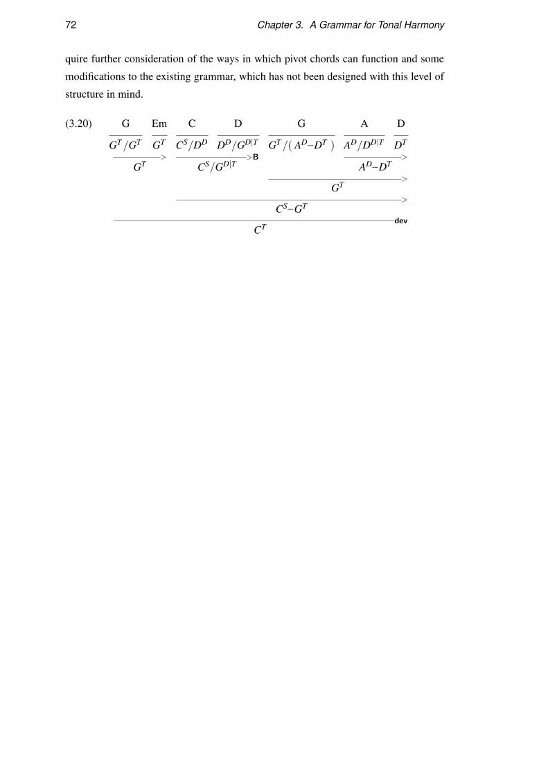
72 Chapter 3. A Grammar for Tonal Harmony
quire further consideration of the ways in which pivot chords can function and some
modifications to the existing grammar, which has not been designed with this level of
structure in mind.
(3.20) G Em C D G A D
GT/GT GT CS/DD DD/GD|T GT/( AD–DT ) AD/DD|T DT
> >B >
GT CS/GD|T AD–DT
>
GT
>
CS–GT
devCT
CHAPTER 4Building an Annotated Corpus
4.1 Introduction
This chapter describes the construction of a corpus of jazz chord sequences annotated
with grammatical analyses using the lexicon and combinatory rules presented in chap-
ter 3. It is common in NLP to use human-annotated datasets to train statistical models
of the parsing process and to use the statistics to guide and speed up the parsing pro-
cess. We shall see in the following chapters how some such techniques from NLP can
be adapted to the music parsing task. Annotated resources serve two purposes: training
the statistical models and testing them to find out how well they can automatically pro-
duce the human annotations. It is common to divide datasets into two parts for these
two purposes, often with a third development (or validation) division used as test data
to compare models during system development.
Whilst some annotated musical datasets exist, none was suitable for training the
current parsing models. Among the most commonly used is the Essen Folksong Col-
lection (Schaffrath & Huron, 1995), a corpus of melodies of European folksongs, with
phrase boundaries annotated, but without harmonic analyses. Temperley (2007) uses
the Kostka-Payne corpus containing metrical and chordal harmonic analyses for 46
short excerpts from tonal music from the common practice era, excerpts and analyses
due to Kostka & Payne (2004). The pieces included do not typically exhibit the sort of
73

74 Chapter 4. Building an Annotated Corpus
hierarchical structures that provide the motivation for the grammatical formalism we
propose. Moreover, the harmonic annotations consist of chord roots only, so, where
such structure does exist, it is not made explicit in the annotations. Other authors, in-
cluding Kroger et al. (2008) and Sapp (2007), use corpora of music by J. S. Bach. As
with the Kostka-Payne corpus, annotations are only in the form of chord roots and lack
further explicit information about hierarchical harmonic structure.
In the absence of any suitable existing corpus, the models described in the follow-
ing chapters are trained on a new corpus of chord sequences annotated with harmonic
analyses. This chapter describes the new corpus of jazz chord sequences and the pro-
cess of annotating them with gold-standard harmonic analyses in a form suitable for
training statistical models in chapter 5. The corpus consists of 76 annotated sequences,
totalling roughly 3,000 chords.
It is worth noting that it is becoming increasingly common in NLP to make use of
unsupervised statistical methods, in which models are trained using unlabelled data,
without annotations of the output that the model should ideally produce and semi-
supervised methods, which use a mix of labelled and unlabelled data or data annotated
with only partial information about the intended output. It would have seemed pre-
mature to explore the application of such learning strategies to harmonic analysis in
the present work, but the models used do have some extensions to unsupervised or
semi-supervised scenarios and in the case of the parsing models this is an active field
of current research.
The dataset is available to download from:
http://jazzparser.granroth-wilding.co.uk/JazzCorpus.
4.2 Chord Sequence Data
4.2.1 Data Format
To train the statistical parsing models, I collected and annotated a small corpus of
jazz chord sequences. The sequences are taken from lead sheets transcribed for jazz
performers to play from.
Table 4.1 shows the data structure used to store each chord. Each chord sequence
is stored as a list of chords, along with the name of the song, the time signature and the
main key1. The roots of the chords are stored as equally tempered pitch classes: that is,
1 Time signature and key do not play a role in any of the models described in this thesis, but were

4.2. Chord Sequence Data 75
Field Description
Root Integer pitch class of transcribed chord root (0, . . . ,11),
relative to the main key
Type Main chord type (tetrad) symbol, chosen from a small
vocabulary (e.g. ‘’, ‘m’, ‘M7’)
Additions (optional) Any further transcribed tones added to the chord, but
not included in the type symbol (e.g. ‘[13’)
Bass (optional) Pitch class of a bass note, if one is given in the chord
symbol (e.g. the B in ‘CM7/B’)
Duration Duration of the chord in beats
Table 4.1: Fields of the data structure used to store each chord in the jazz corpus.
chords rooted on A[ and G] are represented identically in the corpus. Correct enhar-
monic spelling is informative to harmonic analysis (Rohrmeier & Graepel, 2012), but
is excluded from this dataset for two reasons. Firstly, the enharmonic spelling of chord
roots (and melodies) in jazz lead sheets is unreliable and is likely to be misleading
if used as a guide for harmonic analysis. Unlike on classical scores, spelling choices
are often made on the basis of ease of reading for performers, an issue almost entirely
orthogonal to decisions about tonality. Secondly, instead of being considered as a con-
straint on harmonic analysis, enharmonic spelling is treated here as a problem that can
be solved using a harmonic analysis of pitch class-based input. The same approach is
taken by Rohrmeier (2011). This paves the way for extension of the automatic analysis
techniques to take input in the form of symbolic performance data (as demonstrated
in chapter 6) or audio recordings of performances, in which such enharmonic spelling
information is not available. All pitch classes in the chord data structure are given
relative to the key. This is purely for ease of annotation; none of the models in chap-
ter 5 relies on knowing the key of its input and all are invariant under transposition.
Some example chords, decomposed into their representation in the corpus, are given
in table 4.2.
included in case they turn out to be of use in future.

76 Chapter 4. Building an Annotated Corpus
Chord symbol Root Type Additions Bass Duration
E[M7 0 M7 4
Dø7 11 %7 2
Gaug7 4 aug7 2
Cm7 9 m7 4
F7 2 7 4
B[7 7 7 2
Fm7/C 2 m7 9 2
D[m6 10 m 6 2
B[7/D 7 7 11 2
E[6 0 6 4
Table 4.2: Example representation of a chord sequence in the jazz corpus, taken from
the beginning of All the Way.
4.2.2 Cross-Validation
Corpora for supervised training of statistical models are typically divided into two
parts: a training set, used to train the models, and a smaller test set, only ever used
at the end of training to report the models’ performance on unseen data. Often a third
division is made: a development set, used during the development of the models to test
them on data that was not in the training set without compromising the test set, which
is maintained strictly as unseen data until the final experiments. Due to its small size,
the jazz corpus contains no heldout test set or development set. Instead, models are
tested using cross-validation. Each experiment is run 10 times2, using 910 of the data
to train the model and the remaining 110 to evaluate the trained model. This means that
the full corpus is used for evaluation, but no model is tested on the same data that was
used to train it.
It is important to stress that, whilst this reduces the problem of over-fitting models
to their training data, it is not a satisfactory alternative to using completely unseen test
data. Over-fitting still occurs, as models are generally tested repeatedly during devel-
opment and selected or parameterized in response to the results. For example, in the
2 The number of divisions of the dataset may vary, but 10-fold cross-validation, used here, is acommon choice. Another commonly used strategy is leave-one-out cross-validation, in which the modelis tested on every entry in the dataset, each time training on the full dataset minus that entry.
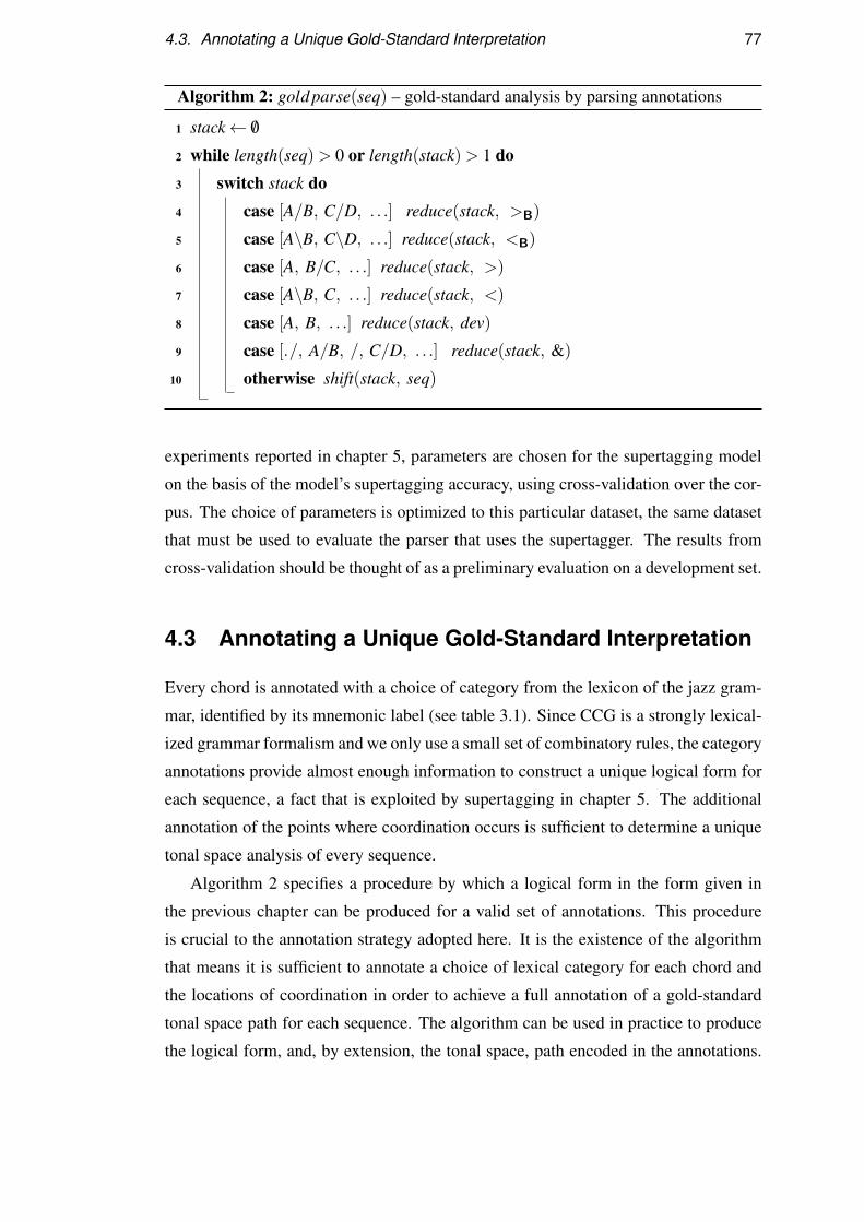
4.3. Annotating a Unique Gold-Standard Interpretation 77
Algorithm 2: gold parse(seq) – gold-standard analysis by parsing annotations
1 stack← /0
2 while length(seq)> 0 or length(stack)> 1 do3 switch stack do4 case [A/B, C/D, . . .] reduce(stack, >B)
5 case [A\B, C\D, . . .] reduce(stack, <B)
6 case [A, B/C, . . .] reduce(stack, >)
7 case [A\B, C, . . .] reduce(stack, <)
8 case [A, B, . . .] reduce(stack, dev)
9 case [./, A/B, /, C/D, . . .] reduce(stack, &)
10 otherwise shift(stack, seq)
experiments reported in chapter 5, parameters are chosen for the supertagging model
on the basis of the model’s supertagging accuracy, using cross-validation over the cor-
pus. The choice of parameters is optimized to this particular dataset, the same dataset
that must be used to evaluate the parser that uses the supertagger. The results from
cross-validation should be thought of as a preliminary evaluation on a development set.
4.3 Annotating a Unique Gold-Standard Interpretation
Every chord is annotated with a choice of category from the lexicon of the jazz gram-
mar, identified by its mnemonic label (see table 3.1). Since CCG is a strongly lexical-
ized grammar formalism and we only use a small set of combinatory rules, the category
annotations provide almost enough information to construct a unique logical form for
each sequence, a fact that is exploited by supertagging in chapter 5. The additional
annotation of the points where coordination occurs is sufficient to determine a unique
tonal space analysis of every sequence.
Algorithm 2 specifies a procedure by which a logical form in the form given in
the previous chapter can be produced for a valid set of annotations. This procedure
is crucial to the annotation strategy adopted here. It is the existence of the algorithm
that means it is sufficient to annotate a choice of lexical category for each chord and
the locations of coordination in order to achieve a full annotation of a gold-standard
tonal space path for each sequence. The algorithm can be used in practice to produce
the logical form, and, by extension, the tonal space, path encoded in the annotations.

78 Chapter 4. Building an Annotated Corpus
During the process of manual annotation, the algorithm can be used as a sanity-checker
for the annotations: a failure of the algorithm to find a full parse or a failure of any of
the rule applications carried out in each of the reductions indicates that there is an error
in annotation3.
The algorithm produces a single gold-standard analysis of any chord sequence fully
annotated with a choice of lexical schema for each chord and chords which occur at
the end of the first constituent of a coordination and those at the end of the second. It
defines deterministic rules for a shift-reduce parser (Kozen, 1997, pp. 181–190) based
on the form of each category (atomic, backward slash or forward slash) and whether
the next input chord is marked as the end of a coordination constituent. The parser
works left to right and greedily performs forward function composition wherever pos-
sible, applying the result to an atomic category when it is reached. This does not rule
out any possible correct results, since any result that can be produced by function ap-
plication alone can also be produced using function composition first, then function
application. Furthermore, the result of coordinating two constituents and then com-
posing with a preceding category (an order which would be excluded by the current
strategy) produces a result identical to that produced by first composing the category
with the first constituent and then performing coordination. This can be seen in ex-
ample 4.1. The logical forms are omitted, but are also identical, due to the reduction
defined in section 3.2.4.
(4.1) A7 Dm7 A[7
AD/DD|T DD/GD|T DD/GD|T
>B
AD/GD|T
&AD/GD|T
A7 Dm7 A[7
AD/DD|T DD/GD|T DD/GD|T
&DD/GD|T
>B
AD/GD|T
The algorithm maintains a stack of categories and iterates, at each step either reduc-
ing the categories on the top of the stack (the left end) or adding the next category from
the annotations onto the stack. The reduction applies one of the rules from section 3.4.1
(identified by its symbol) and replaces the categories on the stack with the single result-
ing category. It does not need to check the syntactic types of the categories other than to
determine whether each is a backward slash category, forward slash category or atomic
category. The function reduce() combines the top two categories using a grammati-
cal rule. The algorithm assumes that this application will succeed without performing
3 Success of the algorithm does not, of course, guarantee that the analysis found is that that wasintended by the annotator, but at least ensures that the corpus contains no nonsensical annotations.

4.3. Annotating a Unique Gold-Standard Interpretation 79
G7 ./ C7 F7 . . . G7 / C
GD/CD|T CD/FD|T FD/B[D|T GD/CD|T CT
>B
CD/CD|T
&GD/CD|T
>
GD–CT
(a)
G7 ./ C7 F7 . . . G7 / C
GD/CD|T CD/FD|T FD/B[D|T GD/CD|T CT
>B×GD/FD|T
>B
GD/CD|T
>
GD–CT
(b)
Figure 4.1: An example that demonstrates the necessity of annotations to mark the
midpoint between two constituents that should be coordinated. The checks on the
form of the syntactic types in algorithm 2 in the absence of the ./ and / annotations
would lead to the composition of the first two cadential chords, as in (b), instead of the
intended interpretation, given by (a). (The two result in the same syntactic type, but a
different semantics.) In this (rather extreme) case, even checking the syntactic types
themselves would not prevent composition. The ./ ensures that the composition made
in (b) is forbidden.
the necessary checks on the syntactic types: failure implies an error in the annotations
which would prevent a full derivation. In addition to the categories themselves, the an-
notations include the special symbols ./, after each category marked by the annotator
as the end of the first constituent of a coordination, and /, after each marked as the end
of the second constituent. The markings are included in figure 4.1, showing how they
ensure that the algorithm performs derivation (a). A category marked as being both (as
happens where more than two constituents are coordinated) is followed by first / and
then ./.
Lines 4–9 define the conditions under which the categories on the top of the stack
are reduced. Although line 4 performs the composition of C/D with A/B4 it does not
4 This might seem back to front, but A/B is the category most recently added to the stack.

80 Chapter 4. Building an Annotated Corpus
check that A=D. Any time categories of this form are seen adjacent to one another, the
only combinatory rule that can combine them is forward composition. The ordering
of the argument conditions ensures that all possible reductions are performed on the
categories on the stack before a new category is shifted. Finally, if no further reductions
can be applied and the input is not exhausted, line 10 shifts the next input category onto
the stack.
The algorithm terminates once all of the categories in the annotations have been
shifted onto the stack and the stack has been reduced to a single category. If there
are no more categories to be shifted, but all reductions are applied and more than one
category remains on the stack, the shift() in line 10 will fail, indicating that there is
an error in the annotations. The algorithm is deterministic and produces exactly one
analysis (by one derivation). This means that, given soundness and completeness of
the algorithm, any valid set of annotations corresponds to a unique harmonic analysis.
A formal proof of soundness and completeness of the algorithm will not be pre-
sented in full here, but could be constructed according to the following form. Proving
soundness involves showing that, if the algorithm produces an analysis from a pairing
of a chord sequence and its annotations, that analysis must be a valid interpretation
permitted by the annotations, and that it is unique. This part of the proof is trivial.
Each of the reductions corresponds to the combination of two adjacent categories by
a grammatical rule and succeeds only if that rule application is permissible under the
grammar. Line 9 is the only reduction that processes the coordination annotations and
it ensures that the coordination rule is used on the constituents they delimit. Since the
algorithm is deterministic, allowing only one derivation, any successful termination
must yield a single legal grammatical interpretation.
Proving completeness involves showing that, if a set of annotations is valid – that is,
if there exists some valid derivation from its lexical categories obeying the constraints
on coordination – the algorithm will find a derivation of the full sequence. A proof
can be constructed by considering in turn each case in which the algorithm could fail,
either by attempting to use an inapplicable rule or by leaving more than one item on
the stack once the entire input is consumed, and showing that there must have been an
error in the annotations – that is, that there is no possible derivation that observes the
constraints of the annotations. For example, consider the first reduction, on line 4:
case [A/B, C/D, . . .] reduce(stack, >B)
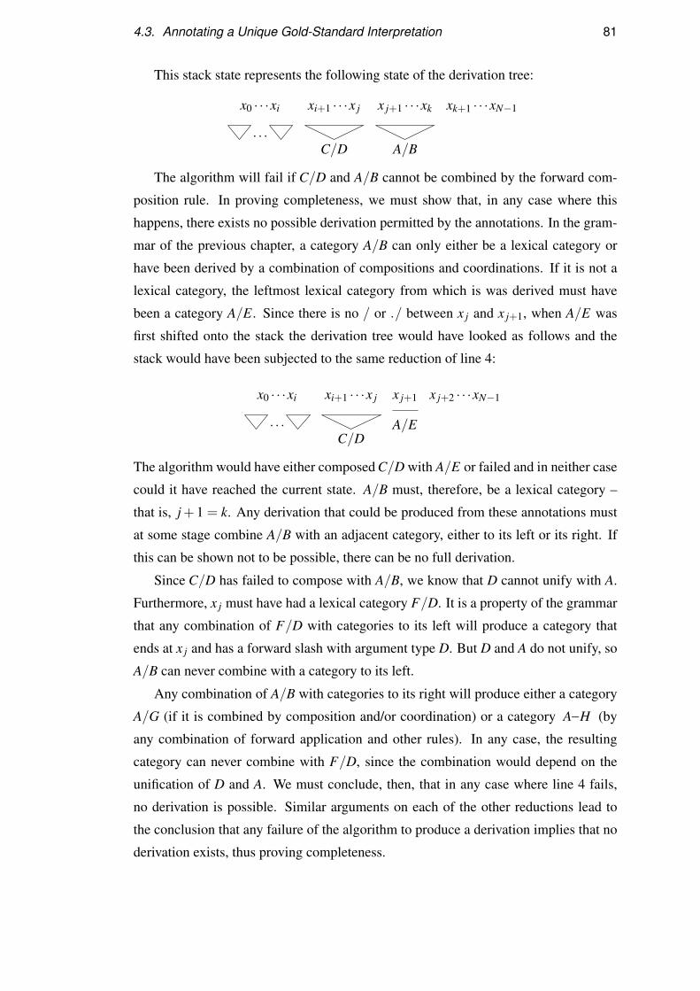
4.3. Annotating a Unique Gold-Standard Interpretation 81
This stack state represents the following state of the derivation tree:
x0 · · ·xi xi+1 · · ·x j x j+1 · · ·xk xk+1 · · ·xN−1
· · ·C/D A/B
The algorithm will fail if C/D and A/B cannot be combined by the forward com-
position rule. In proving completeness, we must show that, in any case where this
happens, there exists no possible derivation permitted by the annotations. In the gram-
mar of the previous chapter, a category A/B can only either be a lexical category or
have been derived by a combination of compositions and coordinations. If it is not a
lexical category, the leftmost lexical category from which is was derived must have
been a category A/E. Since there is no / or ./ between x j and x j+1, when A/E was
first shifted onto the stack the derivation tree would have looked as follows and the
stack would have been subjected to the same reduction of line 4:
x0 · · ·xi xi+1 · · ·x j x j+1 x j+2 · · ·xN−1
· · · A/EC/D
The algorithm would have either composed C/D with A/E or failed and in neither case
could it have reached the current state. A/B must, therefore, be a lexical category –
that is, j+1 = k. Any derivation that could be produced from these annotations must
at some stage combine A/B with an adjacent category, either to its left or its right. If
this can be shown not to be possible, there can be no full derivation.
Since C/D has failed to compose with A/B, we know that D cannot unify with A.
Furthermore, x j must have had a lexical category F/D. It is a property of the grammar
that any combination of F/D with categories to its left will produce a category that
ends at x j and has a forward slash with argument type D. But D and A do not unify, so
A/B can never combine with a category to its left.
Any combination of A/B with categories to its right will produce either a category
A/G (if it is combined by composition and/or coordination) or a category A–H (by
any combination of forward application and other rules). In any case, the resulting
category can never combine with F/D, since the combination would depend on the
unification of D and A. We must conclude, then, that in any case where line 4 fails,
no derivation is possible. Similar arguments on each of the other reductions lead to
the conclusion that any failure of the algorithm to produce a derivation implies that no
derivation exists, thus proving completeness.

82 Chapter 4. Building an Annotated Corpus
Example 4.2 is a cadence from Alfie, using the annotations from the corpus. The
annotations include the markers of points of coordination ./ and /. The series of shift
and reduce operations carried out by the algorithm on this input is shown in table 4.3.
(4.2) CM7
CT
Dm7
CT\CT
Em7
ED/AD|TA7
AD/DD|TDm7
DD/GD|TG7
GD/CD|T ./
Em7
ED/AD|T
A7
AD/DD|TDm7
DD/GD|T ./
E[◦7
AD/DD|TDm7
DD/GD|T /
Gaug7
GD/CD|T /
CM7
CT
4.4 Annotation Procedure
I annotated each chord sequence in the corpus with a single analysis. Each chord
received a single lexical schema, chosen from the lexicon of table 3.1, and any chord
might be marked as the end of a non-final coordination constituent, the end of a final
coordination constituent, or both. Once a sequence was fully annotated, it was parsed
using the annotations according to algorithm 2 by way of a sanity check to detect errors
preventing a normal-form derivation. Furthermore, the result of a successful parse was
examined to ensure that the interpretation was that that was intended.
Ultimately, a decision about a chord’s function or a tension-resolution dependency
must be made on the basis of intuition. Conceivably, some of these decisions could
be made (or at least constrained) on the basis of enharmonic pitch spelling of score
notation or chord roots, reflecting the reading of the composer or transcriber. Two
problems stand in the way of this. Firstly, most chord root motion is by cadences,
along the horizontal dimension of the tonal space. As a result, the most common tonal
ambiguity is between notes separated by the syntonic comma – (4,−1) in the tonal
space – which is not distinguished by pitch spelling. For example, if we were able to
distinguish a dominant seventh tone from a minor seventh tone of a chord we would
know whether the chord has a dominant function. However, pitch spelling leaves us
in the dark as far as this distinction is concerned. Secondly, jazz lead sheets prioritize
ease of reading for performers over music theory. Consequently, even where pitch
spelling in chord roots or melodies appears to give clues as to functional analysis, they
cannot be relied on. The annotation procedure, then, must rely on a lengthy process
of repeatedly listening to recordings, playing from the lead sheets and experimenting
with substitutions and other harmonic modifications that are dependent on particular
interpretations.

4.4. Annotation Procedure 83
Operation Stack
1. Shift CT
2. Shift CT , CT\CT
3. Reduce < CT
4. Shift CT , ED/AD|T
5. Shift CT , ED/AD|T , AD/DD|T
6. Reduce >B CT , ED/DD|T
7. Shift CT , ED/DD|T , DD/GD|T
8. Reduce >B CT , ED/GD|T
9. Shift CT , ED/GD|T , GD/CD|T
10. Reduce >B CT , ED/CD|T
11. Shift CT , ED/CD|T , ./
12. Shift CT , ED/CD|T , ./, ED/AD|T
13. Shift CT , ED/CD|T , ./, ED/AD|T , AD/DD|T
14. Reduce >B CT , ED/CD|T , ./, ED/DD|T
15. Shift CT , ED/CD|T , ./, ED/DD|T , DD/GD|T
16. Reduce >B CT , ED/CD|T , ./, ED/GD|T
17. Shift CT , ED/CD|T , ./, ED/GD|T , ./
18. Shift CT , ED/CD|T , ./, ED/GD|T , ./, AD/DD|T
19. Shift CT , ED/CD|T , ./, ED/GD|T , ./, AD/DD|T , DD/GD|T
20. Reduce >B CT , ED/CD|T , ./, ED/GD|T , ./, AD/GD|T
21. Shift CT , ED/CD|T , ./, ED/GD|T , ./, AD/GD|T , /
22. Reduce & CT , ED/CD|T , ./, ED/GD|T
23. Shift CT , ED/CD|T , ./, ED/GD|T , GD/CD|T
24. Reduce >B CT , ED/CD|T , ./, ED/CD|T
25. Shift CT , ED/CD|T , ./, ED/CD|T , /
26. Reduce & CT , ED/CD|T
27. Shift CT , ED/CD|T , CT
28. Reduce > CT , ED–CT
29. Reduce dev CT
Table 4.3: The series of shift and reduce operations carried out by the algorithm on a
cadence from Alfie.
84 Chapter 4. Building an Annotated Corpus
Harmonic analysis is both somewhat subjective and somewhat ambiguous: of the
many conceivable analyses of a particular piece, some people will hear one whilst oth-
ers another; and there are circumstances where multiple possible analyses may be con-
sidered simultaneously plausible. (Indeed, this is frequently exploited by composers
to disorient listeners.) These are two distinct difficulties for annotation and must be
considered separately.
The problem of subjectivity gives rise to two specific annotation problems: agree-
ment between multiple listeners (annotators) and consistency between analyses pro-
duced by the same listener on different hearings. The first, annotator agreement, can
be measured by involving multiple annotators, each being given a set of inputs to an-
notate such that each input is annotated by several annotators. The second, annotator
consistency, can be measured by asking the same annotator to annotate the same input
again a suitable length of time after the first occasion and measuring the agreement
between the two analyses. Both procedures require a large amount of additional time
and expense, measurement of annotator agreement in particular, since it involves train-
ing multiple annotators. For this reason, I have not attempted to measure annotator
agreement in this work. We must bear in mind, therefore, that the models presented
in chapter 5 are being trained to reproduce the analyses of one individual listener and
that others’ hearings might differ. Measuring annotator consistency, on the other hand,
is a simpler matter. An experiment to judge the annotation consistency is described in
section 4.5.1.
The ambiguity of harmonic analysis is elegantly modelled by the present grammat-
ical approach. Ambiguities of interpretation can be reflected in the choice of lexical
categories and some of the choices of rule application during the derivation process.
For example, different lexical categories interpret a chord as having a dominant or sub-
dominant function, or as a dominant function chord subjected to a tritone substitution.
Decisions about where cadences are left unresolved and which chord eventually sup-
plies their resolution are made by the choice of in what order to apply the combinatory
rules, in particular when the coordination rule is used. The parser described in chap-
ter 5 uses an algorithm that maintains multiple possible interpretations of the chord
sequence at any particular point in the parsing process. A probabilistic model asso-
ciates weights with the alternative interpretations. In this way, a notion of ambiguity is
built into the interpretative mechanism which, given a suitable probabilistic model, em-
ulates the ambiguity of human interpretation. A similar approach to modelling musical
ambiguity is suggested by Jackendoff (1991). When annotating gold-standard deriva-

4.4. Annotation Procedure 85
tions, however, for practical reasons, only one analysis of any particular sequence is
included in the corpus5. Many ambiguities that exist when only a part of a chord se-
quence has been heard are later resolved and it is the resulting final resolution that the
annotations represent. In order to produce the same interpretation, a parser will often
have to allow for local ambiguities – multiple interpretations of a part of the sequence
– of which many will later turn out to be incompatible with other parts of the sequence.
Much of the time, of the remaining ambiguities in a final interpretation, one may be
selected as preferred, as in the Autumn Leaves example of section 2.6.5.
4.4.1 Analysis Decisions
In the process of annotating a chord sequence the annotator must choose a particular
analysis of the harmonic structure by deciding the function of each chord, the substitu-
tion if one is used and the role that the chord plays in the harmonic structure. Certain
principles can be established to help resolve difficult cases of ambiguity, introduced
below by means of an example. It is important to be aware that the annotation deci-
sions discussed below are the conclusion of a process of playing and listening to the
music in question. Some decisions require extensive consideration and experimenta-
tion, whilst others barely warrant discussion. That is not to say that the interpretation
falls unambiguously out of a simple algorithmic analysis, but merely that the intuitions
of a listener familiar with the style of music lead to a strong preference for a particular
interpretation.
Let us consider again example 4.2, repeated here in example 4.3 with the names of
lexical entries used for each chord, chosen from the lexicon of table 3.1.
(4.3) CM7
Ton
CT
Dm7
Colour-IIb
CT\CT
Em7
Dom
ED/AD|T
A7
Dom
AD/DD|T
Dm7
Dom
DD/GD|T
G7
Dom
GD/CD|T ./
Em7
Dom
ED/AD|T
A7
Dom
AD/DD|T
Dm7
Dom
DD/GD|T ./
E[◦7
Dom-tritone
AD/DD|T
Dm7
Dom
DD/GD|T /
Gaug7
Dom
GD/CD|T /
CM7
T
CT
5 Marcus et al. (1993) describe the inclusion of a small amount of ambiguity in the annotation of alinguistic treebank corpus, motivated by a wish to avoid forcing annotators to make arbitrary decisionsin cases of genuine linguistic ambiguity. The ambiguity is limited to permitting multiple part-of-speechtags for individual words and specific attachment ambiguities in syntactic trees, in which one attachmentis chosen as preferred.
86 Chapter 4. Building an Annotated Corpus
Much of the annotation here is uncontroversial, given the treatment of extended ca-
dence structures introduced in chapter 2 and the corresponding grammar of chapter 3.
The first and last chords are tonics of the main key of the piece, so are interpreted using
the Ton schema. Most of the remaining chords are dominant function chords without
substitution, interpreted using the Dom schema, which covers not only a primitive
dominant function but also the extended, recursive function. Their function is strongly
signalled by the addition of the dominant seventh note in each case and the sequence
of downward fifths between roots leads to a clear extended dominant function in each
of the cadential constituents – [Em7 A7 Dm7 G7], [Em7 A7 Dm7] and [Dm7 Gaug7].
The E[◦7 prepares the Dm7 and serves the same harmonic function as an A7 would.
The use of the Dom-tritone schema may seem odd, since this is a much weaker form
of substitution than a tritone substitution: it is in fact merely an inversion an A◦7 chord
and is only written with an E[ root for the performer’s convenience. The grammar’s
lexicon, however, does not include a separate schema for each of the three inversions
of a diminished seventh chord with this interpretation. If schemata were added for
these, they would have both identical syntactic types and identical logical forms to the
schemata for dominant substitutions (Dom-backdoor, Dom-tritone and Dom-bartok).
The inverted A◦7 chord, then, may be interpreted using the Dom-tritone schema.
The addition of annotations to mark points of coordination force the derived struc-
ture to treat the G7 chord’s resolution as delayed until the final tonic (thanks to the
/ preceding the tonic) and the penultimate Dm7’s resolution as momentarily delayed
until the Gaug7.
There remains now one major ambiguity. The Dm7 after the first chord could be
interpreted in two quite different ways. It could be treated as an extended dominant,
using the Dom category, followed by a ./ to delay its resolution until after [Em7 A7
Dm7]. Alternatively, it can be treated (as in these annotations) as a substitute for an F
chord, a small excursion to the subdominant prior to the cadence, comparable to the
IV chord in the common I IV I elaboration of a tonic. In this case, it is no easy matter
to decide between the two quite plausible analyses and the decision to annotate the
latter should not be taken to claim that the other is wrong. In fact, the decision was
made after a lengthy process of playing the chords on a piano with the tune, trying a
variety of alternative substitutions that would be permitted by each interpretation. The
eventual result was a weak preference for the reading given. However, cases with this
degree of difficulty in annotator interpretation are relatively rare, the majority of the
material being closer to the remainder of this example.
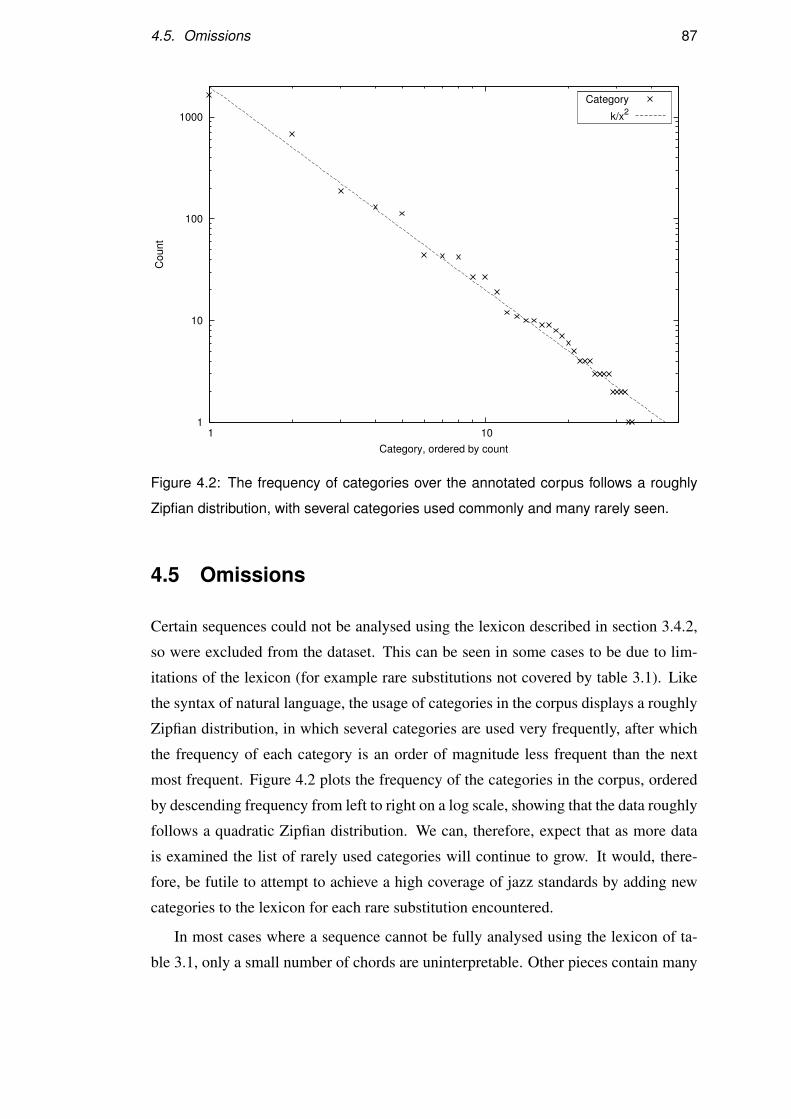
4.5. Omissions 87
1
10
100
1000
1 10
Count
Category, ordered by count
Category
k/x2
Figure 4.2: The frequency of categories over the annotated corpus follows a roughly
Zipfian distribution, with several categories used commonly and many rarely seen.
4.5 Omissions
Certain sequences could not be analysed using the lexicon described in section 3.4.2,
so were excluded from the dataset. This can be seen in some cases to be due to lim-
itations of the lexicon (for example rare substitutions not covered by table 3.1). Like
the syntax of natural language, the usage of categories in the corpus displays a roughly
Zipfian distribution, in which several categories are used very frequently, after which
the frequency of each category is an order of magnitude less frequent than the next
most frequent. Figure 4.2 plots the frequency of the categories in the corpus, ordered
by descending frequency from left to right on a log scale, showing that the data roughly
follows a quadratic Zipfian distribution. We can, therefore, expect that as more data
is examined the list of rarely used categories will continue to grow. It would, there-
fore, be futile to attempt to achieve a high coverage of jazz standards by adding new
categories to the lexicon for each rare substitution encountered.
In most cases where a sequence cannot be fully analysed using the lexicon of ta-
ble 3.1, only a small number of chords are uninterpretable. Other pieces contain many
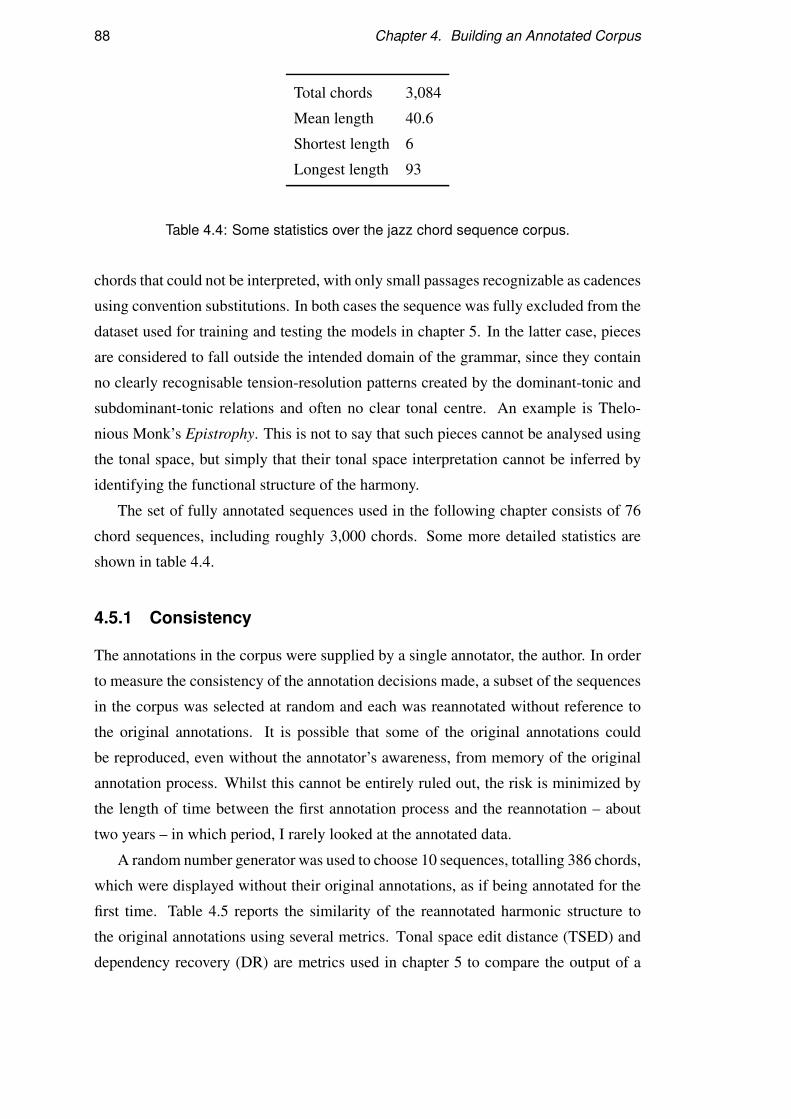
88 Chapter 4. Building an Annotated Corpus
Total chords 3,084
Mean length 40.6
Shortest length 6
Longest length 93
Table 4.4: Some statistics over the jazz chord sequence corpus.
chords that could not be interpreted, with only small passages recognizable as cadences
using convention substitutions. In both cases the sequence was fully excluded from the
dataset used for training and testing the models in chapter 5. In the latter case, pieces
are considered to fall outside the intended domain of the grammar, since they contain
no clearly recognisable tension-resolution patterns created by the dominant-tonic and
subdominant-tonic relations and often no clear tonal centre. An example is Thelo-
nious Monk’s Epistrophy. This is not to say that such pieces cannot be analysed using
the tonal space, but simply that their tonal space interpretation cannot be inferred by
identifying the functional structure of the harmony.
The set of fully annotated sequences used in the following chapter consists of 76
chord sequences, including roughly 3,000 chords. Some more detailed statistics are
shown in table 4.4.
4.5.1 Consistency
The annotations in the corpus were supplied by a single annotator, the author. In order
to measure the consistency of the annotation decisions made, a subset of the sequences
in the corpus was selected at random and each was reannotated without reference to
the original annotations. It is possible that some of the original annotations could
be reproduced, even without the annotator’s awareness, from memory of the original
annotation process. Whilst this cannot be entirely ruled out, the risk is minimized by
the length of time between the first annotation process and the reannotation – about
two years – in which period, I rarely looked at the annotated data.
A random number generator was used to choose 10 sequences, totalling 386 chords,
which were displayed without their original annotations, as if being annotated for the
first time. Table 4.5 reports the similarity of the reannotated harmonic structure to
the original annotations using several metrics. Tonal space edit distance (TSED) and
dependency recovery (DR) are metrics used in chapter 5 to compare the output of a

4.5. Omissions 89
Metric Precision Recall F-score
TSED 99.07 98.76 98.91
DR 99.38 99.69 99.53
AA 98.16 98.16 98.16
Table 4.5: Similarity between reannotated chord sequences and the original annota-
tions measured by the TSED and DR of the harmonic analyses and the AA.
parser that uses the grammar of chapter 3 to the annotated gold-standard harmonic
structure. They measure the similarity of the harmonic structure implied by the anno-
tations, TSED by the closeness of the interpretation as a path through the tonal space,
DR by the accuracy of the tonal relations. For a full description of the metrics, see
section 5.3.7.
A third metric, anotation accuracy (AA), measures directly the accuracy of the
annotated lexical categories and points of coordination. The accuracy of the choice
of lexical categories can be simply measured as the proportion of chords for which
the same lexical category was chosen in the two annotations. A point of coordination
(middle or end) can be annotated on any chord, but in practice only occurs on a small
number chords in each sequence. An f-score measure can be computed to cover both
types of annotation. The precision P is defined as the number of matching category
choices Catm plus the number of matching points of coordination Coordm, divided by
the total number of chords N and annotated points of coordination in the reannotation
Coordr.
P =Catm +Coordm
N +Coordr
The recall is defined as the same count of matching annotations, divided by the total
number of chords N and annotated points of coordination in the original annotation
Coordo.
R =Catm +Coordm
N +Coordo
The f-score in calculated as the harmonic mean of the P and R. In table 4.5, the recall,
precision and f-score are equal, because the number of annotated points of coordination
happened to be the same in the two annotation sets, even though they did not always
coincide.
The results of the comparison in table 4.5 show that, although several different
annotation decisions were made on a second round of annotations, they were for the

90 Chapter 4. Building an Annotated Corpus
Chord class Categories
X 26
Xm 44
X7 26
Xm7 28
X◦7 28
Table 4.6: The number of lexical schemata that may be used for each chord class. Note
that this includes the repetition schemata derived by the tonic repetition and cadence
repetition unary rules.
most part identical. This suggests that a consistent approach was taken to the annota-
tion procedure. This experiment tells us nothing about how easy it would be to train
more annotators to follow the same procedure and what level of agreement could be
expected between them.
4.6 Lexical Ambiguity
Measuring the lexical ambiguity of chords (or words) under the grammar – how many
categories are available as possible lexical interpretations of each chord – helps to give
some idea of the difficulty of the task faced by the parsing models. Hockenmaier
(2003) reports such figures for a CCG grammar whose lexicon was extracted from
syntactic trees of the Penn Treebank converted into CCG derivations. She found that
each word type has on average 1.7 lexical entries, but in practice the ambiguity is much
higher than this. Measured over the training subset of the corpus, each word has on
average 19.2 entries, because many high-frequency words are highly ambiguous.
The grammar of chapter 3 has a very much smaller lexicon, since the syntactic
constructions handled are more constrained. The total set of lexical categories avail-
able to interpret a particular chord are those derived by instantiating each of the lexical
schemata in table 3.1, plus those generated by expanding the lexicon with the repeti-
tion unary rules, using the root of the chord. A particular chord may not legally be
interpreted by any of this set of categories, but only those for which the chord class (on
the left side of the ‘:=’ in the lexicon) contains the chord’s type.
4.7. Conclusion 91
The number of categories available for each chord class (see table 3.2) is shown in
table 4.6. The average number of categories per chord class is 30.4. Like Hockenmaier,
we can take into account how frequently different chord types occur. The average num-
ber of categories available for each chord in the corpus of chord sequences of chapter 4
is 26.8 (with a standard deviation of 4.3). It is unsurprising that the distribution of chord
types has little effect on the average ambiguity, since the chord types are all projected
onto the small set of chord classes, unlike in the grammar for English of Hockenmaier
(2003), in which the level of ambiguity varies greatly between different words.
Although the number of categories in the lexicon of the present grammar is very
much smaller than those in the lexicon for English (Hockenmaier reports 1,224 dis-
tinct lexical categories), the degree of lexical ambiguity encountered in practice when
parsing chord sequences is comparable.
4.7 Conclusion
The corpus described in this chapter contains chord sequences, of the sort used by jazz
performers as the basis for improvisation, each manually annotated with a harmonic
analysis. Although in some cases multiple analyses may be considered plausible by
different annotators, or even by a single annotator, I have attempted to make systematic
decisions where ambiguities arise. An experiment in which a subset of the corpus was
reannotated shows a high level of consistency in the annotation process.
The annotations are in the form of categories chosen from the lexicon of the gram-
mar in chapter 3, with enough information to specify a unique harmonic analysis,
derivable by a deterministic algorithm that parses the sequence using the annotations.
It is a property of the strongly lexicalized grammar formalism that only a small amount
of information beyond the lexical categories themselves is necessary to define a unique
interpretation.
The annotated corpus can be used to train statistical models for guiding a parser.
Since the corpus includes a full harmonic analysis of each chord sequence, it can also
be used to train a model that derives a harmonic analysis for a chord sequence without
using the grammar, using only the pairing of chord sequences with analyses as training
data. In the next chapter, the corpus is used in both ways, the latter for training a
baseline that does not use a grammar. Since the corpus is small, it contains no heldout
test data. Models must, therefore, be evaluated using cross-validation, reducing but not
eliminating the problem of over-fitting the training data.


CHAPTER 5Statistical Parsing of Chord Sequences
5.1 Introduction
Parsing harmony using the grammar of jazz chord sequences described in chapter 3
suffers from a problem familiar from natural language parsing using similar gram-
mars. The lexical ambiguity – that is, the high level of ambiguity in the interpretation
and structural role of each individual chord – prohibits exhaustive parsing to deliver
every syntactically well-formed interpretation. The grammar restricts the possible in-
terpretations of chords on the basis of their context. A bottom-up parser enforces these
constraints by considering every possible interpretation of each individual chord with
a category permitted by the lexicon and exploring the large space of possible combi-
nations of the categories using the grammar’s rules. Using the jazz grammar, as with
any wide-coverage grammar for natural language, the number of possible derivations
to consider makes exhaustive automatic parsing infeasible for even moderately long
inputs.
For instance, consider example 3.16, repeated here:
(5.1) Gm7 Cm7 B7 B[7 E[6
The first chord, Gm7, was interpreted in example 3.16 using the (extended) dominant
lexical schema (Dom), giving it the category GD/CD|T : λx. leftonto(x). Other pos-
93

94 Chapter 5. Statistical Parsing of Chord Sequences
sible interpretations, however, are permitted by the lexicon. It might, for example,
be interpreted as a tritone substitution (Dom-tritone) or one of the rarer of the class
of ‘Bartok’ substitutions that Elliott (2009) describes (Dom-bartok) and so on. The
parser must consider a variety of categories for the other chords too. Many of these will
quickly prove to be dead-ends. Gm7 and Cm7 may combine into a recursive cadence
if they are both treated using the Dom schema, but not if they adopt the Dom-bartok
and Dom schemata. Some categories which in their immediate context appear nonsen-
sical may turn out to be able to combine with more distant chords. Consider then the
hopelessly implausible, but grammatical, interpretation represented by the derivation
in example 5.2, in which the Gm7 is treated as a Bartok substitution whose resolution
is delayed until the final E[6.
(5.2) Gm7 Cm7 B7 B[7 E[6
B[D/E[D|T CD/FD|T FD/B[D|T B[D/E[D|T ET
>B
CD/B[D|T
>B
CD/E[D|T
&B[D/E[D|T
>
B[D–E[T
Moreover, even if the parser were able to consider all possible grammatical interpreta-
tions, example 5.2 demonstrates a second problem. The parser needs a way to distin-
guish the most plausible among the large number of possible interpretations. It is usual
in NLP to use statistical models based on a corpus of hand-annotated sentences to rank
possible interpretations. The same techniques can also be used to speed up parsing by
eliminating apparently improbable interpretations early in the process.
One technique is to associate a probability model with the parser’s derivations. A
set of alternative analyses can be ranked according to the probability of their deriva-
tions under this model, providing a means to distinguish one analysis (or a small set of
analyses) as the most plausible. The model can also provide a solution to the former
problem of the infeasibility of exhaustive parsing if it is defined compositionally over
intermediate constituents of grammatical derivations: a parsing scheme can be used
that eliminates improbable constituents in early stages of parsing on the basis that they
are unlikely to appear in the most probable full analysis.
Bod (2002b), Honingh & Bod (2005) and Temperley (2007) have shown that some
statistical techniques used in NLP can be applied to tasks in music processing. This
5.2. Supertagging Experiments 95
chapter introduces two types of probabilistic statistical model commonly used for nat-
ural language parsing, applied here to the task of parsing chord sequences. The first,
a supertagger, is aimed primarily at speeding up the process to allow some interpreta-
tion to be found quickly. The second, a model of CCG derivations, adopts the natural
language parsing technique of Hockenmaier & Steedman (2002) and Hockenmaier
(2003). Both models estimate probabilities from statistics over the corpus of chapter 4.
In this chapter, I describe the technique of supertagging as it has been applied
to CCG parsing. An experiment with some simple supertagging models trained on
the jazz corpus explores the effectiveness of the proposed class of models for the
task. I then describe the model proposed by Hockenmaier for parsing natural lan-
guage with CCG and report the results of some experiments to demonstrate the suit-
ability of this model for the chord sequence parsing task. The system used in the
experiments, the Jazz Parser, is a new implementation of an algorithm commonly used
for parsing natural language suitable for processing the grammar of chapter 3, aug-
mented with the parsing models of this chapter. The source code is freely available
from http://jazzparser.granroth-wilding.co.uk. Some of the details of the
parsing models and experiments of this chapter, including closely related experimen-
tal results, have been published previously by Granroth-Wilding & Steedman (2011,
2012b).
5.2 Supertagging Experiments
5.2.1 Supertagging
A problem arises when using a statistical model over the derivations performed by
a parser. Both language and, as we have seen, musical harmony involve structures
that span large passages, featuring dependencies between arbitrarily distant parts of
the input. A parser must maintain a very large number of possible interpretations
of different spans of the input and the parsing model described later in this chapter
can be used to eliminate some of these, whilst keeping those that it considers likely
to be used later in the derivation. It is in the nature of a lexicalized grammar that
there may be a large number of possible interpretations of any individual word (or
here chord). For example, over the corpus of the previous chapter, the jazz chord
grammar was found to permit on average 26.8 categories per chord. The parser uses
its compositional model to reduce this set, but must maintain enough low-probability

96 Chapter 5. Statistical Parsing of Chord Sequences
1 2 3 4 5 6 7 8 9 10 11 12 13
1 25 35 103 365 2k 6k 30k 146k 821k 0 0 0 0
2 27 41 103 425 2k 8k 35k 188k 0 0 0 0
3 27 39 113 394 2k 8k 39k 0 0 0 0
4 25 39 106 367 2k 7k 0 0 0 0
5 27 39 110 393 2k 0 0 0 0
6 25 46 109 380 0 0 0 0
7 27 39 113 0 0 0 0
8 25 39 0 0 0 0
9 27 0 0 0 0
10 23 0 0 0
11 36 0 0
12 12 0
13 25
Figure 5.1: The number of categories in each cell of the chart during an exhaustive
parse of 13 chords from Alfie (seen before with gold-standard categories in exam-
ple 4.2). The parser has so far processed nine chords. Row numbers correspond
to the first word in the span of the cell, column numbers to the last. Numbers on the
diagonal are thus numbers of lexical categories.
interpretations that it is unlikely to eliminate categories that would have proved more
probable once considered in a wider context. The larger the set of local interpretations
that are kept, the longer the parsing process takes. Figure 5.1 shows how the number
of partial interpretations grows as an exhaustive chart parser (see section 5.3.2) works
its way through the sequence. Already, after processing nine chords, it is clear that
parsing the full sequence is going to be infeasible. Supertagging is a statistical method
commonly used for NLP parsing with CCG and other strongly lexicalized grammars
to reduce this problem and find a grammatical interpretation quickly.
A supertagger reduces the number of categories the parser must consider in the
first steps of parsing, typically using a probabilistic sequence model. The technique
was first described by Srinivas & Joshi (1994) for a lexicalized formalism similar to
CCG. Supertagging was first applied to CCG parsing by Clark & Curran (2004a). The
term supertag refers to a lexical item (category) that may be used by the parser as an
analysis of a single word. For the grammar of chapter 3, this is a choice of a lexical

5.2. Supertagging Experiments 97
schema to instantiate at the chord’s root. Although the parser itself could narrow down
the possible categories on the basis of statistics over larger spans later in the parsing
process, supertagging has the benefit of being able to speed up parsing by ruling out
some lexical categories using a sequence model that can be evaluated quickly before
parsing begins.
A bad choice of lexical categories could make it impossible to parse a sequence
at all. The adaptive supertagging (AST, Clark & Curran, 2004a) algorithm allows
categories considered less probable by the supertagger to be used only if necessary
to find a full parse. First, the supertagger is used to assign a small set of categories
to each word according to its model. The parser attempts to find a full parse with
these categories, using a statistical model like that described below. If it succeeds, the
result is returned and no further supertags are considered. If it fails, the supertagger
supplies some more, slightly less probable, categories and the parser tries again. This
is repeated until the parser succeeds or some other termination condition is reached
(for example after a fixed maximum number of iterations). If multiple full parses are
found, the parser’s probability model is used in the usual fashion to rank them.
In this section, I evaluate the effectiveness of n-gram models with a variety of
parameters as supertaggers, predicting the annotated categories for the chord sequences
in the corpus of the previous chapter. I also compare this to a naive use of an existing
supertagger written for NLP parsing. On the basis of the results of these experiments,
in section 5.3 I use a supertagging model in conjunction a statistical parser.
5.2.2 N-Gram Supertagging Models
Markovian sequence models have been extensively used in both language and music
processing for sequence analysis. They are an obvious starting point for building a
chord sequence supertagger. Such models can quickly predict a sequence, or multiple
sequences, of categories for a chord sequence and have a wide array of well-understood
associated techniques for dealing with circumstances where large amounts of training
data are not available.
All the experiments reported here are run using the small dataset described in chap-
ter 4 for training and evaluation. Given the size of the dataset, all models can be ex-
pected to suffer from extreme data sparsity problems. This makes the use of smoothing
of vital importance and, as we shall see, it also limits the potential benefit of using more
complex models. In this section, I describe a series of experiments with variants on a

98 Chapter 5. Statistical Parsing of Chord Sequences
. . . xi−2 xi−1 xi . . .
yi−2 yi−1 yi
P(yi) = P(yi|xi)×P(xi|xi−1)
(a)
. . . xi−2 xi−1 xi . . .
yi−2 yi−1 yi
P(yi) = P(yi|xi)×P(xi|xi−1,xi−2)
(b)
Figure 5.2: HMM structure. (a) Bigram HMM: at each timestep, the observed data yi is
generated from a hidden state xi, chosen from a finite set of possible states. (b) Trigram
HMM: xi depends on xi−1 and xi−2.
basic hidden Markov model (HMM, Rabiner & Juang, 1986), all commonly used in
NLP.
5.2.2.1 Model Structure
The general structure of an HMM is shown in figure 5.2a. HMMs can be applied to
the problem of chord sequence supertagging by treating grammatical categories as the
hidden states of the model and the observed chord sequence as the model’s emissions.
Such a model makes the Markov independence assumption: that the probability dis-
tribution over categories for a particular chord depends on the category assigned to
the previous chord, but not on the categories assigned to earlier chords. Further, the
probability of seeing a particular chord label is assumed to be dependent only on the
current category interpretation and not on any others surrounding it.
Recall from chapter 3 that a grammatical category used as a lexical interpretation of
a chord is arrived at by choosing a schema from the lexicon of table 3.1 and specializing
it to the chord’s root. The states of the model, then, which represent grammatical
categories, can be decomposed into a pair (Schi,SRi) of lexical schema and pitch class
root. The probability of emitting any chord from a state whose root does not match the
chord’s is always zero.
In this model, the Markov assumption has the following effect. The probability
P(CT,CR |Sch,SR) of emitting a sequence of chords with types CT and roots CR,
given a sequence of categories made up of schemata Sch and roots SR = CR, is ap-
proximated by ∏i P(CT i |Schi). The probability P(Schi,SRi |Sch0,...,i−1,SR0,...,i−1) of
generating the next in the sequence of hidden category states (Schi,SRi), is approxi-

5.2. Supertagging Experiments 99
mated by P(Schi,SRi |Schi−1,SRi−1). For example, the first three chords of Alfie (first
seen in example 4.2) would be decomposed as: (M7, C), (m7, D), (m7, E). The state
labels corresponding to the gold-standard categories for these chords are: (Ton, C),
(Colour-IIb, D), (Dom, E). The probability distribution over the choice of category for
Em7 is conditioned on the choice of category for Dm7, but not on the preceding CM7.
Much of the time, these assumptions may be reasonable: a chord may, for exam-
ple, be confidently interpreted as a tonic on the basis that its type is M7 and that the
previous category was interpreted as a dominant a perfect fifth above. However, in
other circumstances the assumptions will be violated: in a coordinated cadence a tonic
resolution of a dominant chord might only be reached some time later.
A generalization of the basic HMM is the n-gram HMM, in which the choice of
state is conditioned not only on the single previous state, but on some longer history
of previous states. The order of such an HMM dictates the length of history on which
each state is conditioned. The basic HMM described above is a first-order, or bigram,
model: the probability of transitioning to a state is conditioned only on the previous
state. An n-gram model is an HMM of order n−1. The structure of a second-order, or
trigram, model is shown in figure 5.2b.
Let us make one further modification to the model’s distributions, motivated by a
musical consideration. A requirement common to most models of music is insensitiv-
ity to absolute pitch: the pitch of a note or chord is meaningful only when considered in
relation to other pitches in the same performance, whilst an entire piece may be trans-
posed up or down without significantly affecting its meaning. It is, therefore, desirable
that the probability distribution over categories should be conditioned on the previously
seen categories only taking into account the relative pitch between the categories. Tran-
sitions between states are modelled as follows: a schema is chosen, conditioned on the
available history of n− 1 schemata, and a root is chosen relative to the previous root,
conditioned on the schema. This is represented in the probability distribution by the δ
function which calculates the interval between two pitch classes: δ(r1,r0) = (r1− r0)
mod 12. A first-order HMM of this kind is represented in figure 5.3.
The model’s transition and emission distributions, then, are as follows:
Ptr-st(Schi,SRi |Schi−n+1,...,i−1,SRi−n+1,...,i−1) =
Ptr-sch(Schi |Schi−n+1,...,i−1)×Ptr-rt(δ(SRi,SRi−1)|Schi)
Pem-st(CT i,CRi |Schi,SRi) =
{Pem-tp(CT i |Schi) if CRi = SRi
0 o/w

100 Chapter 5. Statistical Parsing of Chord Sequences
Sch0,
SR0
Sch1,
SR1. . . SchT−1,
SRT−1
CT0,
CR0
CT1,
CR1
CTT−1,
CRT−1
Ptr-sch(Schi |Schi−1)×Ptr-rt(δ(SRi,SRi−1)|Schi)
Pem-tp(CT i |Schi) if SRi = CRi
Figure 5.3: First-order HMM structure for a supertagging model. The transition distri-
bution is decomposed into a distribution over schemata, conditioned on the previous
schema, and a distribution over roots, relative to the previous root. The emission distri-
bution is defined over chord types, conditioned on the schema and is non-zero only for
categories with a root matching the chord.
An HMM is decoded by choosing the sequence of states S that generates the ob-
served data O with maximum probability1:
argmaxS
(P(S,O)) = argmaxS
(∏
iPtr-st(Si|Si−1,...,i−n+1) ·Pem-st(Oi|Si)
)
This can be computed efficiently using the dynamic programming Viterbi algorithm
(Viterbi, 1967; first applied to NLP by Vintsyuk, 1968). Alternatively, we may com-
pute the set of most probable categories for each observed chord using the forward-
backward algorithm (as detailed by Rabiner, 1989). For adaptive supertagging, it is
this latter decoding that is required.
The advantage of an n-gram model of order higher than one is that it is able to cap-
ture frequent patterns of hidden states over a wider window of context. A disadvantage
is that data sparsity becomes a greater problem: in any training dataset, the higher n is
the fewer examples of each n-gram of states will be found. One commonly used solu-
tion to this is introduced in section 5.2.2.3. Since the jazz corpus is small, it contains
too few examples of even the most frequent patterns to support models of order much
larger than bigram.
The experiments reported below evaluate the performance of several orders of n-
gram HMM. The simplest possible model is a unigram model, in which no context is
taken into consideration at all. I report results for unigram, bigram and trigram models.
1 Note that the roots of the categories are fixed by the observed chord sequence, since any stateswith roots not matching the chords have zero emission probability. Decoding, therefore, involves just achoice of schema for each chord: argmaxSch(P(Sch,O)).

5.2. Supertagging Experiments 101
Whilst higher-order models could be used, these results show that data sparsity already
has a heavy impact on the bigram and trigram models.
5.2.2.2 Training
All models are trained using supervised maximum likelihood training over the labelled
corpus described in chapter 4. Each distribution is estimated by maximum likelihood
estimation on the basis of counts of the frequency of events in the corpus: P(A|B) is
estimated by Count(A,B)Count(B) . As is common in NLP (for example Clark & Curran, 2004a),
counts of very rare events are considered untrustworthy, so a threshold is set below
which Count(A,B) is treated as 0.
The parameters of an HMM can also be trained on unlabelled data using the
expectation-maximization (EM) algorithm (Baldridge, 2008 for example uses this
method to train an HMM supertagger). Given unlabelled chord sequences, a model
trained using supervised estimation could be retrained so as to increase the likelihood
of the new chord data. The present experiments do not use this technique, since no
unlabelled data is currently readily available. In principle, however, it would not be
difficult to gather unlabelled chord sequences and this could present a promising solu-
tion to the problems of data sparsity.
5.2.2.3 Backoff and Smoothing
Statistical models of natural language commonly face a problem of data sparsity, due
to the Zipfian nature of many aspects of natural languages. Chapter 4 showed that the
distribution of lexical categories in the corpus follows a roughly Zipfian distribution,
meaning that we can expect severe data sparsity problems with this small training
set and that adding more training data will improve our coverage of rare events with
diminishing returns.
Several techniques are commonly used with n-gram models to deal with this prob-
lem. One is Katz backoff (Katz, 1987). The n-gram model uses counts of all state
sequences xi−n+1, . . . ,xi and xi−n+1, . . . ,xi−1 seen in the training data in order to es-
timate the probability P(xi|xi−1, . . . ,xi−n+1). To avoid assigning a zero probability to
sequences xi−n+1, . . . ,xi which have not been seen in the training data, the probabilities
are smoothed. The probabilities of seen events are scaled down, or discounted slightly
and the remaining probability mass is reserved for unseen events. The probability
of an unseen event is then computed by backing off to a lower-order model condi-

102 Chapter 5. Statistical Parsing of Chord Sequences
tioned on a smaller context, which is more likely to have been seen in the training data.
The probability P(xi|xi−1, . . . ,xi−n+1) is estimated as P(xi|xi−1, . . . ,xi−n+2) (trigram
P(xi|xi−1,xi−2), for instance, backs off to bigram P(xi|xi−1)), scaled by a normalizing
factor so that the probability mass reserved by discounting is distributed among the
unseen events according to the lower-order model. Backoff may continue recursively
until the event is found in the training data or the unigram model is reached. The ad-
vantage of Katz backoff is that it allows a higher-order model to be used only where
counts are available to estimate its probabilities and a lower-order model in all other
cases.
Various suitable discounting techniques can be used to perform the necessary
smoothing for Katz backoff. Laplace smoothing is a straightforward technique, by
which one count is added to all events, including those never seen, and the probabili-
ties are computed from the adjusted counts. Good-Turing estimation (Good, 1953) is
a discounting technique commonly used in NLP. It works well with large datasets, but
requires care when used with limited data. Many variants exist to deal with this prob-
lem (Gale & Sampson, 1995). A simpler method is used here. Witten-Bell smoothing
(Bell et al., 1990) uses a discounting function that computes the amount of probability
mass to reserve for unseen events on the basis of how many of the seen events occur
only rarely. The experiments below include both Laplace and Witten-Bell smoothing.
5.2.3 Using the C&C Supertagger
The supertagging models described above are specific to the interpretation of chord
sequences. It is also possible to use an existing supertagger designed for supertag-
ging as part of a linguistic parser. Clark & Curran (2004a) demonstrated the use of
supertagging for parsing with CCG. Their implementation of a supertagger and sta-
tistical parser, the C&C parser, is publicly available2. The supertagger can be used
independently of the parser, via the msuper tool, to suggest categories from a lexicon
with associated probabilities according to a trained model.
The C&C supertagger uses maximum-entropy feature-based log-linear models to
assign CCG categories to the words of a sentence. It uses a variety of contextual
features to predict categories for words and each of the possible features receives a
weight during training. A model can easily be trained on any training data given in a
suitable form. It can be used as a supertagger for chord input by training it to assign
2 http://svn.ask.it.usyd.edu.au/trac/candc, accessed Dec 2012.
5.2. Supertagging Experiments 103
categories chosen from the lexicon of table 3.1 to chord sequence data preprocessed
to represent the chord’s root relative to the previous root, rather than at its absolute
pitch. This has the effect of making the model insensitive to absolute pitch, a property
that was enforced in the n-gram models by modelling root intervals in the transition
distribution. The supertagger can be made to return a probability for each possible
category allowing the parser to run the AST algorithm. The Jazz Parser can use the
output from a call to msuper in the same way it uses the state occupation probabilities
from the n-gram models. In comparisons with the models below, the C&C supertagger
used in this way will be referred to as CANDC.
5.2.4 Evaluation
A supertagging model is used to help the parser by selecting a small set of categories
for each input word. Ultimately, its performance can only be evaluated on the basis of
the effect its choice of categories has on the parser’s accuracy.
The accuracy of a supertagger’s highest weighted choice of category for each chord
against a human-annotated gold standard may not give a good indication of its perfor-
mance when coupled with a parser. For example, a choice of categories that allows
the parser to produce a full, but poor quality, interpretation of the sequence is more
useful to the parser than a choice that matches the gold standard on a high proportion
of chords, but cannot lead to a full parse. This holds even more strongly when using
the AST algorithm, which allows the parser to request lower probability categories
from the supertagger if it cannot find a parse using those considered most probable.
In this case, we do not know how far down the list of categories provided by the su-
pertagger the parser will go before it finds a full parse, so evaluating the accuracy of
the supertagger’s top category sequence may not be meaningful.
Nevertheless, the ideal approach of evaluating competing supertagging models by
the effect they have on parsing accuracy is impractical, since parsing the full corpus
is a time-consuming process. It is, therefore, useful to have some evaluation metrics
with which to compare supertagging models independently of the parser. I consider
here some metrics which allow us to compare the performance of supertaggers quickly
without having to run the parser in every case.
Using AST, the parser may request more categories from the supertagger if it can-
not find a full parse. Consider a second metric, n-best accuracy, which measures
the proportion of chords for which the gold-standard category is found among the n
104 Chapter 5. Statistical Parsing of Chord Sequences
highest-weighted categories returned by the supertagger. For a small value of n (say
3 or 4), this is likely to be a truer indication of supertagger’s performance. As n in-
creases, the metric becomes more generous, but we do not know how many categories
the parser will request before terminating. Instead, measuring the cross entropy be-
tween the gold-standard selection of categories and the supertagger’s distribution, Ps,
over categories rewards models that give higher probability to the gold-standard cate-
gories.
Let us consider the gold-standard distribution over categories, Pg, to be that in
which the gold-standard category receives a probability of 1 and all others 0. The
cross entropy of this distribution with Ps is the arithmetic mean of the negative log
probabilities assigned by the model to the gold-standard categories. A lower value
means that the correct categories were on average given a higher probability, so lower
is better.
The cross entropy of Pg and Ps is defined as:
H(Pg,Ps) =−∑x
Pg(x) log(Ps(x))
Since the gold-standard distribution is 0 over all categories other than the gold-standard
category, this value is− log(Ps(Schi)), where Schi is the gold-standard category choice.
Averaging this over all the chords in all the sequences of the test set gives the cross
entropy per chord:
H =− 1N ∑
ilog(Ps,i(Schi))
In evaluating the supertagging models, I will report both 1-best accuracy and cross
entropy. The corpus contains no separate training and testing sets, so evaluation is
performed using 10-fold cross validation (see section 4.2.2).
5.2.5 Results
Figures 5.4 and 5.5 compare n-gram supertagging models for a range of settings of each
parameter. The experiment explores a variety of combinations of parameter settings to
see how the supertagger’s performance is affected. Models of three orders are included:
unigram (state probabilities conditioned on no context), bigram (a standard HMM) and
trigram (state probabilities conditioned on two previous states).
In each case, Katz backoff is used for events with zero counts. Bigram models back
off to unigram and trigram models back off to bigram and then to unigram. Different
values of the low-count threshold (cutoff ) are tried – the value below or equal to which
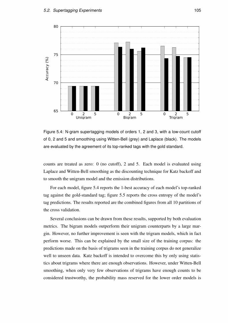
5.2. Supertagging Experiments 105
65
70
75
80
0 2 5 0 2 5 0 2 5
Acc
ura
cy (
%)
TrigramBigramUnigram
Figure 5.4: N-gram supertagging models of orders 1, 2 and 3, with a low-count cutoff
of 0, 2 and 5 and smoothing using Witten-Bell (grey) and Laplace (black). The models
are evaluated by the agreement of its top-ranked tags with the gold standard.
counts are treated as zero: 0 (no cutoff), 2 and 5. Each model is evaluated using
Laplace and Witten-Bell smoothing as the discounting technique for Katz backoff and
to smooth the unigram model and the emission distributions.
For each model, figure 5.4 reports the 1-best accuracy of each model’s top-ranked
tag against the gold-standard tag; figure 5.5 reports the cross entropy of the model’s
tag predictions. The results reported are the combined figures from all 10 partitions of
the cross validation.
Several conclusions can be drawn from these results, supported by both evaluation
metrics. The bigram models outperform their unigram counterparts by a large mar-
gin. However, no further improvement is seen with the trigram models, which in fact
perform worse. This can be explained by the small size of the training corpus: the
predictions made on the basis of trigrams seen in the training corpus do not generalize
well to unseen data. Katz backoff is intended to overcome this by only using statis-
tics about trigrams where there are enough observations. However, under Witten-Bell
smoothing, when only very few observations of trigrams have enough counts to be
considered trustworthy, the probability mass reserved for the lower order models is

106 Chapter 5. Statistical Parsing of Chord Sequences
1
1.5
2
0 2 5 0 2 5 0 2 5
Entr
opy
TrigramBigramUnigram
Figure 5.5: N-gram supertagging models of orders 1, 2 and 3, with a low-count cutoff
of 0, 2 and 5 and smoothing using Witten-Bell (grey) and Laplace (black). The models
are evaluated by the entropy of its predicted tag distribution (lower values are better).
small. The result is that using a higher order model is detrimental where the training
data does not provide enough examples, even when Katz backoff is used. This might
also explain why the low-count cutoff does not help the performance. Where only a
small number of categories have been seen in a particular context, the trigram model
assigns a high probability to them and scales down the bigram probabilities greatly
when backing off. As the threshold is increased, the model backs off more often, but
scales the probabilities from the backoff model down more, giving a higher weight to
its estimates of events it has seen. The results suggest that models of higher orders will
fare still worse on this small dataset.
Models using Witten-Bell smoothing perform better than those with the simpler
Laplace smoothing, except where the low-count cutoff is high. Given the sparsity of
the training data, it is unsurprising that the models benefit from a more sophisticated
smoothing technique. There are other commonly used smoothing techniques that have
not been tested here which could improve performance. For example, Kneser-Ney
smoothing is widely used in NLP, either for backoff, like the smoothing techniques
discussed above, or as a means of interpolating the estimates from different models.

5.3. Statistical Parsing Experiments 107
Model Entropy Accuracy (%)
BESTNGRAM 1.13 77.11
CANDC 1.39 80.22
Table 5.1: Comparison of the best n-gram supertagging model (bigram, no low-count
cutoff, Witten-Bell smoothing) to CANDC.
The best performing n-gram model by both metrics is the bigram model using
Witten-Bell smoothing with no low-count cutoff. Table 5.1 compares this model,
BESTNGRAM, to CANDC. CANDC achieves slightly higher top-tag accuracy, but the
bigram model scores better on the entropy metric. The C&C supertagger is evidently
dealing well with the sparse data. The entropy result indicates that the bigram model is
on average assigning a higher probability to the gold-standard tag. It should be noted
that the C&C supertagger was used only with its default settings and that it is highly
likely that better results could be achieved by a careful choice of parameters. In the
parsing experiments below, the bigram BESTNGRAM model is used.
5.3 Statistical Parsing Experiments
5.3.1 Introduction
In this section, I discuss the application of a model of CCG derivations introduced
for natural language parsing by Hockenmaier & Steedman (2002) and Hockenmaier
(2003). The model is trained on human-annotated CCG derivations for some set of
inputs. It uses statistics over local parts of the derivations to estimate the probability
of different ways of combining categories during a new derivation.
5.3.2 CKY Parsing
A wide variety of parsing algorithms have been described for natural language parsing.
I shall focus on one algorithm here, the Cocke-Kasami-Younger (CKY, Harrison, 1978)
algorithm, since it has been shown to have good time complexity for the class of gram-
mar formalisms containing CCG and has been extensively used in practice for CCG

108 Chapter 5. Statistical Parsing of Chord Sequences
Algorithm 3: CKY parsing algorithm for CCG, as given by Steedman (2000)
1 for j← 1 to n do2 t( j, j)←{A|A is a lexical category for a j}3 for i← j−1 down to 0 do4 for k← i down to 0 do5 t(i, j)← pack{A|for all B ∈ t(k, i),C ∈ t(i+1, j).
such that B C ⇒ A for some combinatory rule in R
and admissible(B C ⇒ A)}
parsing (Auli, 2012). CKY is a bottom-up chart parsing algorithm originally designed
for context-free grammars and applied to CCG by Vijay-Shanker & Weir (1990).
The CKY algorithm uses a chart to store multiple possible interpretations for each
subspan of the input. The Jazz Parser uses the adaptation of the algorithm to CCG
presented by Steedman (2000). The algorithm, without the probabilistic extensions
described below, is reproduced in algorithm 3. The jth input token (word or, here,
chord) is denoted by a j. The chart, t, is a data structure that contains an entry t(i, j)
for every possible subspan of the input that begins with the ith token and ends with the
jth. The function pack stores a category, consisting of syntactic type and logical form,
in the chart in a data structure holding one entry per syntactic type. The applicability
of further rules to a category at a later stage of the derivation will depend only on
its syntactic type. The admissible function performs any necessary tests to decide
whether the category A resulting from a rule application should be included in the
chart. For CCG, admissible cannot simply exclude any category A for which another
already exists in the chart with the same syntactic type, as it may in the case of context-
free grammars, but, because of CCG’s spurious ambiguity (discussed below), must
also check that the existing category does not contain a logical form equivalent to A’s
(Karttunen, 1989).
The algorithm proceeds as follows. The index j points to the end of the span being
considered and moves from left to right through the sentence. Each time a new token
is covered by j, all lexical categories for that token are added to the chart (line 2).
For each token, the index i moves backwards through the preceding tokens, so that
the span (i+ 1, j) always represents a subsequence of the tokens so far encountered
ending at the jth, considering all such subsequences. For each such span, the index k
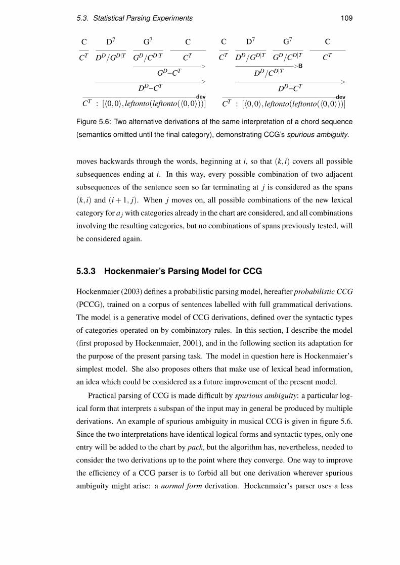
5.3. Statistical Parsing Experiments 109
C D7 G7 C
CT DD/GD|T GD/CD|T CT
>
GD–CT
>
DD–CT
devCT : [〈0,0〉, leftonto(leftonto(〈0,0〉))]
C D7 G7 C
CT DD/GD|T GD/CD|T CT
>B
DD/CD|T
>
DD–CT
devCT : [〈0,0〉, leftonto(leftonto(〈0,0〉))]
Figure 5.6: Two alternative derivations of the same interpretation of a chord sequence
(semantics omitted until the final category), demonstrating CCG’s spurious ambiguity.
moves backwards through the words, beginning at i, so that (k, i) covers all possible
subsequences ending at i. In this way, every possible combination of two adjacent
subsequences of the sentence seen so far terminating at j is considered as the spans
(k, i) and (i+ 1, j). When j moves on, all possible combinations of the new lexical
category for a j with categories already in the chart are considered, and all combinations
involving the resulting categories, but no combinations of spans previously tested, will
be considered again.
5.3.3 Hockenmaier’s Parsing Model for CCG
Hockenmaier (2003) defines a probabilistic parsing model, hereafter probabilistic CCG
(PCCG), trained on a corpus of sentences labelled with full grammatical derivations.
The model is a generative model of CCG derivations, defined over the syntactic types
of categories operated on by combinatory rules. In this section, I describe the model
(first proposed by Hockenmaier, 2001), and in the following section its adaptation for
the purpose of the present parsing task. The model in question here is Hockenmaier’s
simplest model. She also proposes others that make use of lexical head information,
an idea which could be considered as a future improvement of the present model.
Practical parsing of CCG is made difficult by spurious ambiguity: a particular log-
ical form that interprets a subspan of the input may in general be produced by multiple
derivations. An example of spurious ambiguity in musical CCG is given in figure 5.6.
Since the two interpretations have identical logical forms and syntactic types, only one
entry will be added to the chart by pack, but the algorithm has, nevertheless, needed to
consider the two derivations up to the point where they converge. One way to improve
the efficiency of a CCG parser is to forbid all but one derivation wherever spurious
ambiguity might arise: a normal form derivation. Hockenmaier’s parser uses a less

110 Chapter 5. Statistical Parsing of Chord Sequences
X
w
P(exp = leaf|X)
P(w|X ,exp = leaf)
X
H
P(exp = unary|X)
P(H|X ,exp = unary)
X
H D
P(exp = left|X)
P(H|X ,exp = left) P(D|X ,exp = left,H)
Figure 5.7: Three of the four types of local trees in Hockenmaier’s model of CCG deriva-
tions, with the probabilities that are multiplied to compute the local tree’s probability.
strict form of this approach. Non-normal form derivations are not forbidden by the
parser, but the PCCG is constructed in such a way that it will in general prefer the
normal form derivation. She defines a systematic normal form for derivations and uses
this form of the analyses in the training data to train the distributions of parsing model
using maximum likelihood estimation.
The parsing model is defined over binary- and unary-branching derivation trees. A
probability distribution is associated with each node in a candidate derivation over its
children. The distribution is based on the syntactic types of the parent and children, but
does not take into account the combinatory rule by which the children are generated
from their parent3.
The probability of a derivation tree is computed from the product of the proba-
bilities of its local trees – each individual node and its children. A node in the tree
may generate a word (leaf), a single child (unary branch) or a pair of children (binary
branch). In the case of a binary branch, one of the two children is designated the head
and the other the non-head, so that the model can be easily extended to capture lexical
head dependencies. The probability of a local tree with parent X , expansion type exp,
head daughter H (if not a leaf), non-head daughter D (if a binary branch) and word w
(if a leaf) is the product of the following probabilities:
• Expansion probability: P(exp|X), probability of expansions leaf, unary, left
(left-head binary branch) and right (right-head binary branch)
3 Although the chart-parsing algorithm with which the model is used operates bottom-up from thewords of the sentence, since it is a generative model the probability distributions are defined in a top-down fashion from the root of the derivation tree to the surface form (sentence).

5.3. Statistical Parsing Experiments 111
• Head probability: P(H|X ,exp), if exp 6= leaf
• Non-head probability: P(D|X ,exp,H), if exp ∈ {left,right}
• Lexical probability: P(w|X ,exp), if exp = leaf
Figure 5.7 shows the products of probabilities for three of the four types of local
tree (right expansion is trivially the mirror image of left expansion).
The parsing model computes the joint probability of a tree (that is, a particular
derivation) and the words observed at its leaves as the product of all the local tree
probabilities. It can also compute the same for a subtree corresponding to a partial
derivation of a subsequence of the input – the inside probability of that subtree. The
model serves two functions in the parsing process. Firstly, it provides a ranking of the
interpretations output by the parser on the basis of the probabilities of their derivations.
The probability of a full interpretation is computed by summing the probabilities of
each of the derivations that led to it. Secondly, it can be used to allow the parser to
perform a more efficient search for a full interpretation by eliminating unpromising
partial interpretations early on. During parsing, the inside probability is computed for
each partial interpretation that is inserted into the chart by summing the probabilities
from all the derivations that led to it. The probability of the subtree must also take
into account the probability that the parent node features in a derivation in the first
place – the outside probability. This is approximated in Hockenmaier’s model by the
unconditioned probability of the parent node P(X), also estimated from the training
corpus. A beam is applied to every span in the chart: when all categories have been
computed for the span, those with a probability below a certain threshold are thrown
away.
The inside probabilities are computed efficiently following the same dynamic pro-
gramming strategy as the CKY parsing algorithm itself. The probability of a new
category added to the chart as a result of applying a rule is computed as the product
of the local tree probabilities for the rule application, the inside probabilities of the
trees rooted at the rule’s arguments (the subtrees of H and D in figure 5.7) and the
estimated outside probability. Since CKY operates bottom-up from the sentence, all
possible derivations leading to the arguments have already been computed, and their
probabilities summed, by the time the rule is applied. The category’s probability value
is added to the probabilities of any other derivation adding the same category to the
same chart edge.

112 Chapter 5. Statistical Parsing of Chord Sequences
5.3.4 PCCG for Parsing with the Jazz Grammar
The PCCG parsing model of Hockenmaier (2003) described above can be applied di-
rectly to parsing using the musical grammar. This section describes a model suitable
for parsing with the music grammar and the details of the smoothing and beaming
techniques implemented for the experiments in section 5.3.8.
5.3.4.1 Probability Distributions
The distributions that comprise the model are identical to Hockenmaier’s, except for
one alteration. Hockenmaier’s model makes a distinction between expansions in which
the left daughter is classified as the head and those where the right is the head. It is
not clear that a notion of lexical head information like that used in Hockenmaier’s
model would be useful to the present parsing task, so the parsing model for the jazz
grammar abandons this distinction. The jazz grammar uses no unary rule (other than
the repetition lexical expansion rules, which do not feature in derivations). The only
expansions the model needs to consider are, therefore, LEAF and BINARY.
The distributions, then, become:
• Expansion probability: P(exp|X), probability of expansions leaf, binary
• Left probability: P(L|X ,exp), if exp = binary, probability of left category L
• Right probability: P(R|X ,exp,L), if exp = binary, probability of right cate-
gory R
• Lexical probability: P(c|X ,exp), if exp = leaf, probability of chord c
The distributions are trained using counts from the corpus of normal-form deriva-
tions by maximum likelihood estimation.
5.3.4.2 Normal-Form Derivations
Following Hockenmaier (2003), the parser is trained on a set of normal-form deriva-
tions. Algorithm 2 in section 4.3 prescribes a way of producing a gold-standard anal-
ysis corresponding to the annotations for a chord sequence in the chord corpus. The
same algorithm serves as a specification of a normal form for derivations. There is
nothing inherent in either the grammar or the form the annotations take that requires
this particular normal form and alternative algorithms could be given as specification
5.3. Statistical Parsing Experiments 113
of others. However, certain features of the jazz grammar mean that this normal form is
particularly simple to specify.
There is one noteworthy respect in which this normal form differs from Hocken-
maier’s. Hockenmaier’s normal form uses the function application rule by preference
and type-raising and function composition only when there exists no alternative deriva-
tion using function application (for example when a constituent formed by composition
must be coordinated). She justifies this decision on the basis that constructions that re-
quire composition are less common than those that permit a function application-only
derivation. The normal form defined by algorithm 2 takes almost the opposite strat-
egy. It proceeds incrementally, greedily performing forward composition wherever
it can and only applies the composed category to its argument (its resolution) at the
end. The reason for this is that sequences of forward-facing cadence categories can al-
ways be combined by composition first and must be where they are to be coordinated,
but function application is never required to take place before composition. Backward-
facing slash categories are also combined greedily with their arguments, resulting in an
application-first derivation, but these are rare and almost never subject to composition.
It is interesting to note that this normal form favours a maximally incremental
derivation under the grammar as it stands. Incremental derivation is of interest to the-
ories of grammar for reasons of cognitive plausibility as well as for practical reasons
(Roark, 2001; Collins & Roark, 2004). Steedman (2000) argues for the use of com-
binatory grammars on the basis that they permit a strong link between competence
and performance (Chomsky, 1965), a version of the Strong Competence Hypothesis of
Bresnan & Kaplan (1982). However, it is a considerably more difficult affair to build
a strictly incremental parsing scheme for CCG for natural language than it would be
for the present grammar and this is a subject of current research. Training the parsing
model on derivations in the particular normal form used here has the advantage over
other possible normal forms that it will encourage the parser to perform incremental
derivations where a choice exists.
5.3.4.3 Smoothing
The parsing model could be presented with a combination of syntactic types that has
never been seen in the training data. The parsing model uses Witten-Bell smoothing
(seen previously in section 5.2.2.3) to assign some small probability to all such unseen
events. This smoothing technique relies on knowing the number of possible events.
Although CCG in general has an infinite number of possible categories, complex cate-

114 Chapter 5. Statistical Parsing of Chord Sequences
85
90
95
100
0 5 10 15 20
Dependency r
ecovery
f-s
core
(%
)
Max categories, m
α = 0.5
α = 0.1
α = 0.01
α = 0.001
m = 1
Figure 5.8: Dependency recovery of parser with an HMM supertagger over eight inputs
from the chord corpus using a range of beam settings. α is the maximum ratio between
the highest and lowest probabilities of categories in any cell. m is a limit on the number
of categories in any cell. When m = 1, α has no effect.
gories in the jazz grammar are limited to a single functional argument (that is, a single
slash). The lexicon of table 3.1 limits the number of theoretically possible syntactic
types to a fixed number, making it possible to use Witten-Bell smoothing to assign a
small probability to previously unseen combinations of categories.
The parsing models of Hockenmaier (2003) use a backoff technique to assign some
probability to unseen words, but do not use smoothing during derivation in the way I
propose here. Hockenmaier’s parser does not check the validity of combinations of
categories using CCG rules, but instead assign a zero probability to any category com-
binations not seen in the training data. The Jazz Parser must operate with much less
training data. It checks for CCG validity and, in the case of a valid rule application that
has never been observed, assigns the combination some small probability by smooth-
ing.

5.3. Statistical Parsing Experiments 115
0:00
0:30
1:00
1:30
2:00
2:30
3:00
3:30
4:00
0 5 10 15 20
Avera
ge p
ars
e tim
e (
min
s)
Max categories, m
α = 0.5
α = 0.1
α = 0.01
α = 0.001
m = 1
Figure 5.9: Average parse time per sequence using an HMM supertagger over eight
inputs from the chord corpus using a range of beam settings.
5.3.4.4 Beam Search
The parser applies a beam to each span in the chart in the same way as Hockenmaier’s
parser. The beam eliminates partial interpretations that receive a low probability un-
der the model, keeping only a number of more probable interpretations. This allows
efficient parsing, since it limits the number of combinations of categories that must be
considered as input to future rule applications.
A variety of strategies can be used for this kind of beam search. Collins (1999)
applies a threshold probability, defined as a fixed fraction α of the probability of the
most probable interpretation on the span. Any categories with a probability lower than
this threshold are discarded. Note that the higher α is, the tighter the beam – that is,
the fewer alternative categories are entertained. An alternative technique is to set a
threshold m on the number of interpretations that may be stored for any span. The
present parser follows Bodenstab et al. (2011) in using both strategies.
Figures 5.8 and 5.9 show the results of an experiment in which the parser was run
on a small subset of the corpus (eight chord sequences) with a variety of beam settings.
All combinations of α ∈ {0.5,0.1,0.01,0.001} and m ∈ {1,5,10,15,20} were tried.

116 Chapter 5. Statistical Parsing of Chord Sequences
(Note that when m = 1 there is never more than one category on any particular span, so
α has no effect.) Figure 5.8 shows the parser’s accuracy measured by the dependency
recovery f-score evaluation metric (introduced later, in section 5.3.7.2). Figure 5.9
shows the average parse time per chord sequence4.
Increasing the width of the α-beam (decreasing α) improves the accuracy of the
parser up to α = 0.01, but no further gain is seen for α = 0.001. Setting the m-beam
wider (increasing m) has almost no effect on dependency recovery, but does increase
parse times for wide α-beams (0.01 and 0.001). This suggests that when the α-beam is
wide, the m-beam is reducing the number of derivations that the parser must consider,
but that the categories it removes rarely contribute to the top-ranked overall result.
For narrower α-beams, m makes no difference at all: presumably spans rarely have
more than m categories on them after the α-beam has been applied. Unsurprisingly,
the parser performs relatively poorly when it is only allowed to keep the single most
probable category for each span.
Since there is little accuracy gain from higher values of m, there is no point in
using m > 10. There is a considerable gain in accuracy from using a wider α-beam,
up to 0.01, but almost no difference when α = 0.001. Since we do not know how
these results on a small subset of the corpus would generalize to the whole corpus, let
alone to other data, it is safer to use a wider beam setting where the tradeoff between
accuracy and parse times is unclear. In the experiments below, the parser is run using
beam settings of α = 0.01 and m = 10.
5.3.5 Tonal Space Path HMM Baseline
One way to quantify the contribution made by restricting interpretations to those that
are syntactically well formed under the jazz grammar is to construct a baseline model
which assigns interpretations without using the grammar. A tonal space interpretation,
in the form of a path, like those generated from the parser’s output in section 3.2.7 can
be produced directly by a probabilistic sequence model. This can be done using an
HMM structure very similar to that used for the supertagging models described earlier.
The model assigns a tonal space point and harmonic function directly to each chord,
instead of assigning categories to chords, as the supertagger does, and parsing to derive
a tonal space path.
4 Each parse job was run on a 2.6GHz AMD Opteron 6212 CPU.

5.3. Statistical Parsing Experiments 117
D[
F
A
A[
C
E
E[
G
B
B[
D
F]
F
A
C]
C
E
G]
G
B
D]
Figure 5.10: Tonal space analysis for the coordinated cadence G7 E7 A7 Dm7 G7 C. The
initial G7 (square) is followed not by the closest point that equal temperament maps to
E (dashed), but a more distant one, as required for the two G7s resolve to share their
resolution.
A reasonable first approximation to an analysis can be derived by assuming that
no chord substitutions are used and that the tonal space path proceeds by the smallest
possible steps. To be precise, for each chord, a procedure chooses, from the infinite set
of points mapped by equal temperament to the chord’s root, the point that is closest to
the previous point on the path by the Manhattan distance metric. The HMM models
deviations from this naive procedure.
There are two reasons why deviations from the naive path occur. First, it may be
that the correct disambiguation of the equal temperament note is not the point closest
to the previous, as happens at points of coordination, where the resolutions of two
cadences are constrained to be the same. An example is shown in figure 5.10. Second,
it may be that there is a substitution (like the tritone substitution), meaning that the
surface chord’s root is not the root of the chord in the analysis.
The HMM’s state labels consist of three values. The first, the substitution coor-
dinate, is a coordinate between (0,0) and (3,2) and denotes the chord root within its
enharmonic block (see figure 5.11) – in other words, the coordinate after accounting
for substitution, but before projecting from the toroidal space of equal temperament
onto the full tonal space. (0,0) represents a chord root of C (or an enharmonic equiva-
lent – B], etc.). For example, a state with the coordinate (1,0) (G) could be associated
with a D[ chord to interpret it as a tritone substitution5. The second value, the block
coordinate, is a coordinate that denotes the number of enharmonic blocks (see sec-
tion 3.2.2) the chord root must be shifted from the point closest to the previous point
on the path. Most often this is (0,0), since paths proceed most often by small steps in
the tonal space. In this case, of the infinite number of possible coordinates permitted
5 Strictly speaking, this would only be a tritone substitution if a dominant function, D, were alsochosen.
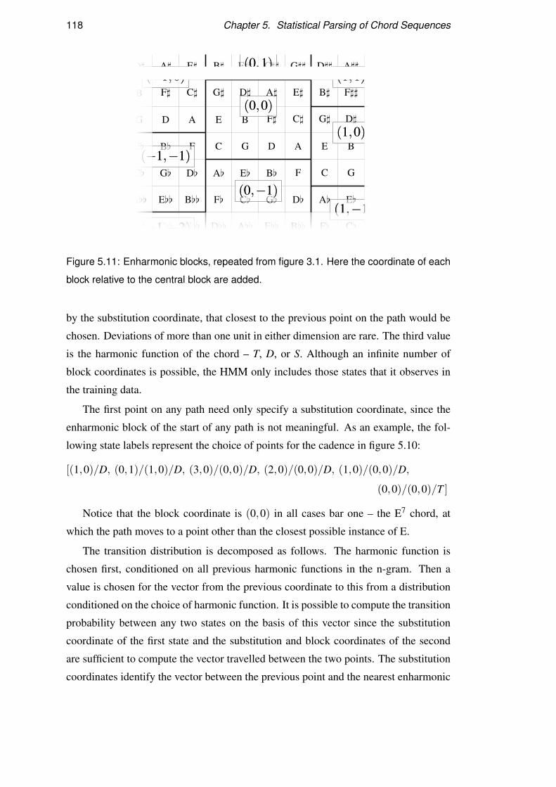
118 Chapter 5. Statistical Parsing of Chord Sequences
F[[
A[[
C[
E[
G
B
D]
C[[
E[[
G[
B[
D
F]
A]
G[[
B[[
D[
F
A
C]
E]
D[[
F[
A[
C
E
G]
B]
A[[
C[
E[
G
B
D]
F]]
E[[
G[
B[
D
F]
A]
C]]
B[[
D[
F
A
C]
E]
G]]
F[
A[
C
E
G]
B]
D]]
C[
E[
G
B
D]
F]]
A]]
G[
B[
D
F]
A]
C]]
E]](0,1)(0,1)
(0,0)(0,0)
(0,−1)(0,−1)
(−1,0)(−1,0)
(−1,−1)(−1,−1)
(−1,−2)(−1,−2)
(1,1)(1,1)
(1,0)(1,0)
(1,−1)(1,−1)
Figure 5.11: Enharmonic blocks, repeated from figure 3.1. Here the coordinate of each
block relative to the central block are added.
by the substitution coordinate, that closest to the previous point on the path would be
chosen. Deviations of more than one unit in either dimension are rare. The third value
is the harmonic function of the chord – T, D, or S. Although an infinite number of
block coordinates is possible, the HMM only includes those states that it observes in
the training data.
The first point on any path need only specify a substitution coordinate, since the
enharmonic block of the start of any path is not meaningful. As an example, the fol-
lowing state labels represent the choice of points for the cadence in figure 5.10:
[(1,0)/D, (0,1)/(1,0)/D, (3,0)/(0,0)/D, (2,0)/(0,0)/D, (1,0)/(0,0)/D,
(0,0)/(0,0)/T ]
Notice that the block coordinate is (0,0) in all cases bar one – the E7 chord, at
which the path moves to a point other than the closest possible instance of E.
The transition distribution is decomposed as follows. The harmonic function is
chosen first, conditioned on all previous harmonic functions in the n-gram. Then a
value is chosen for the vector from the previous coordinate to this from a distribution
conditioned on the choice of harmonic function. It is possible to compute the transition
probability between any two states on the basis of this vector since the substitution
coordinate of the first state and the substitution and block coordinates of the second
are sufficient to compute the vector travelled between the two points. The substitution
coordinates identify the vector between the previous point and the nearest enharmonic

5.3. Statistical Parsing Experiments 119
instance of the current point. The block coordinate then specifies the number of blocks
this must be shifted by to obtain the vector between the two points. Note that this way
of constructing the transition distribution makes it insensitive to transposition.
Ptr-hp(subi, blocki, funi | subi−1, blocki−1, funi−1, . . .) =
Ptr-hp-fn(funi | funi−1, . . .)×Ptr-hp-root(vector(subi−1, subi, blocki) | funi)
The emission distribution is also decomposed. The block coordinate of the state
plays no role in the emission probability distribution. The distribution is once again
made insensitive to absolute pitch by modelling the difference between the pitch class
encoded in the substitution coordinate and the chord root, instead of defining a distribu-
tion over both. In other words, the distribution models the substitution itself, regardless
of the absolute pitch of the chord. The δ function is defined, as in section 5.2.2.1, as the
interval between two pitch classes. The substitution is chosen conditioned on the func-
tion of the state. Then the chord type is chosen, conditioned on both the substitution
and the function.
Pem-hp(CT i, CRi | subi, blocki, funi) =
Pem-hp-root(δ(CRi, subi) | funi)×Pem-hp-type(CT i | δ(CRi, subi), funi)
The baseline model, like the supertagger, is trained using maximum likelihood es-
timation, only this time the training data is chord sequences paired with their annotated
tonal space paths. The model is decoded using the Viterbi algorithm to find a single
optimal sequence of states for a chord sequence. The states are then transformed into
a sequence of tonal space coordinates, with associated harmonic functions.
I shall refer to the baseline model as HMMPATH. Unlike the parser, HMMPATH
assigns some interpretation to any input sequence, since it is not limited to returning
grammatical interpretations.
5.3.6 Aggressive Backoff
The supertagging models described above in section 5.2 used a backoff technique –
Katz backoff – to deal with the problem of data sparsity that arises when training
higher-order n-gram models. A similar idea can be used as a simple way to deal with
the problem of grammar coverage.
The parser fails to find any analysis at all for some inputs. This may happen because
the chord sequence uses substitutions or passing chords not covered by the grammar’s
lexicon or because the correct analysis is erroneously eliminated by the supertagger’s
120 Chapter 5. Statistical Parsing of Chord Sequences
or parser’s beam. Any attempt at manually expanding the lexicon of section 3.4.2 to
reduce this problem is destined to be an uphill struggle. We saw in chapter 4 that the
lexical categories used in the corpus annotations follow roughly Zipfian distribution in
their frequencies. As the lexicon is expanded, we can expect exponentially more train-
ing data to be required to support statistical models such as those discussed above. We
must, therefore, consider other ways of dealing with the lexical coverage problem. Re-
cent parsing literature in NLP has explored techniques for learning new lexical entries
on the basis of an existing lexicon (for example, Thomforde, 2012). Similar approaches
could be applied to expanding the present harmonic grammar, but I shall not consider
this any further here. Instead, let us consider how the parser can deal immediately with
limitations of the lexicon when it encounters passages it cannot interpret.
The baseline model, HMMPATH, described in the previous section provides just
such a possibility. Since the model is not restricted by the grammar to producing well-
formed analyses, it can propose at least some analysis for any input, even where data
sparsity means that its predictions are ill-informed. The analyses it outputs will in
general be of poorer quality than the parser’s output, since it does not have the benefit
of the hand-specified constraints motivated by music theory that are encoded in the
grammar. The backoff technique proposed here, therefore, is to use the baseline model
when the parser cannot find any analysis. If the parser succeeds, its analysis is used;
otherwise, the analysis of HMMPATH is returned instead.
This method ensures that the system is robust, in the sense that it has full coverage
of any input data. However, it is only suitable if the desired output is the tonal space
path analysis. If the logical form itself is required (or its dependency graph represen-
tation), other similarly motivated backoff models can be imagined, taking inspiration,
for example, from the dependency parsing literature. However, I shall not consider any
such model here. For this reason, the results from the model including backoff would
only be able to be evaluated using a metric based on the tonal space path.
Other more subtle backoff techniques could be considered, but are not explored
here. One promising direction for using the present parser in a more robust manner
is to make use of partial parses, found by inspecting the chart after a failed parse.
A simple technique could be used to fill the gaps, assuming a continuation of the
previously established tonal centre or using a local analysis similar to HMMPATH.
This approach is a more satisfactory model of human processing: faced with a tonally
confusing passage of music, humans have no difficulty in picking up the thread again
once a sufficiently clearly interpretable passage is subsequently encountered.
5.3. Statistical Parsing Experiments 121
5.3.7 Evaluation
In order to evaluate the harmonic analyses output by the parser, we must be able to
compute the similarity of an analysis to that specified in the annotated corpus. I shall
propose two metrics to compare analyses and use both in the evaluation experiments
that follow.
5.3.7.1 Tonal Space Edit Distance Evaluation Metric
The first metric compares analyses in the form of paths through the tonal space. Sec-
tion 3.2.7 presented an algorithm to transform a logical form produced by parsing using
the grammar into a sequence of points, relative to some arbitrarily chosen start point,
through the tonal space. The reason for using an evaluation metric based on the parser’s
yield in this form is that a notion of tonal similarity is encapsulated in the Manhattan
distance metric in the space (Longuet-Higgins & Steedman, 1971). Therefore, two
paths through the space that differ only by small divergences denote tonally similar
harmonic analyses. It is not clear that such a metric provides a meaningful measure
of tonal similarity for radically dissimilar paths, such as between an analysis of, say,
the Basin Street Blues and of On Green Dolphin Street. However, in a comparison
between analyses of the Basin Street Blues it should provide a meaningful measure of
the extent of the divergence.
The tonal space distance metric proposed here is computed as the edit distance
between two paths: that is, the smallest number of insertions, deletions or substitutions
of points on one path required to transform it into the other. Edit distance (also known
as Levenshtein distance) can be computed using a dynamic programming algorithm
described by Wagner & Fischer (1974).
A naive metric of this sort would be unjustly harsh on certain types of errors. For
example, if the candidate analysis misinterprets a dominant function chord as a passing
chord, it can end up with a cadence one step shorter than the corresponding cadence
in the gold-standard analysis. In some circumstances, this can result in the remainder
of the path being shifted to a position enharmonically equivalent to the gold-standard
analysis. Instead of penalizing the parser just for the deletion of a leftward step, a
naive metric will end up marking the whole of the rest of the path as incorrect. A
solution is to compare the paths not as a list of coordinates, but as a list of the tonal
relations between consecutive chords. We first transform both paths into a list of the
vectors between pairs of consecutive points and then apply the edit distance metric to
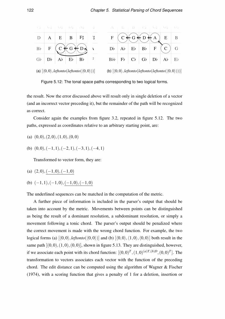
122 Chapter 5. Statistical Parsing of Chord Sequences
G[
B[
D
F]
D[
F
A
C]
A[
C
E
G]
E[
G
B
D]
B[
D
F]
A]
F
A
C]
E]
(a) [〈0,0〉, leftonto(leftonto(〈0,0〉))]
B[[
D[
F
A
F[
A[
C
E
C[
E[
G
B
G[
B[
D
F]
D[
F
A
C]
A[
C
E
G]
E[
G
B
D]
(b) [〈0,0〉, leftonto(leftonto(leftonto(〈0,0〉)))]
Figure 5.12: The tonal space paths corresponding to two logical forms.
the result. Now the error discussed above will result only in single deletion of a vector
(and an incorrect vector preceding it), but the remainder of the path will be recognized
as correct.
Consider again the examples from figure 3.2, repeated in figure 5.12. The two
paths, expressed as coordinates relative to an arbitrary starting point, are:
(a) (0,0),(2,0),(1,0),(0,0)
(b) (0,0),(−1,1),(−2,1),(−3,1),(−4,1)
Transformed to vector form, they are:
(a) (2,0),(−1,0),(−1,0)
(b) (−1,1),(−1,0),(−1,0),(−1,0)
The underlined sequences can be matched in the computation of the metric.
A further piece of information is included in the parser’s output that should be
taken into account by the metric. Movements between points can be distinguished
as being the result of a dominant resolution, a subdominant resolution, or simply a
movement following a tonic chord. The parser’s output should be penalized where
the correct movement is made with the wrong chord function. For example, the two
logical forms (a) [〈0,0〉, leftonto(〈0,0〉)] and (b) [〈0,0〉,〈1,0〉,〈0,0〉] both result in the
same path [(0,0),(1,0),(0,0)], shown in figure 5.13. They are distinguished, however,
if we associate each point with its chord function: [(0,0)T ,(1,0)(a)T,(b)D,(0,0)T ]. The
transformation to vectors associates each vector with the function of the preceding
chord. The edit distance can be computed using the algorithm of Wagner & Fischer
(1974), with a scoring function that gives a penalty of 1 for a deletion, insertion or
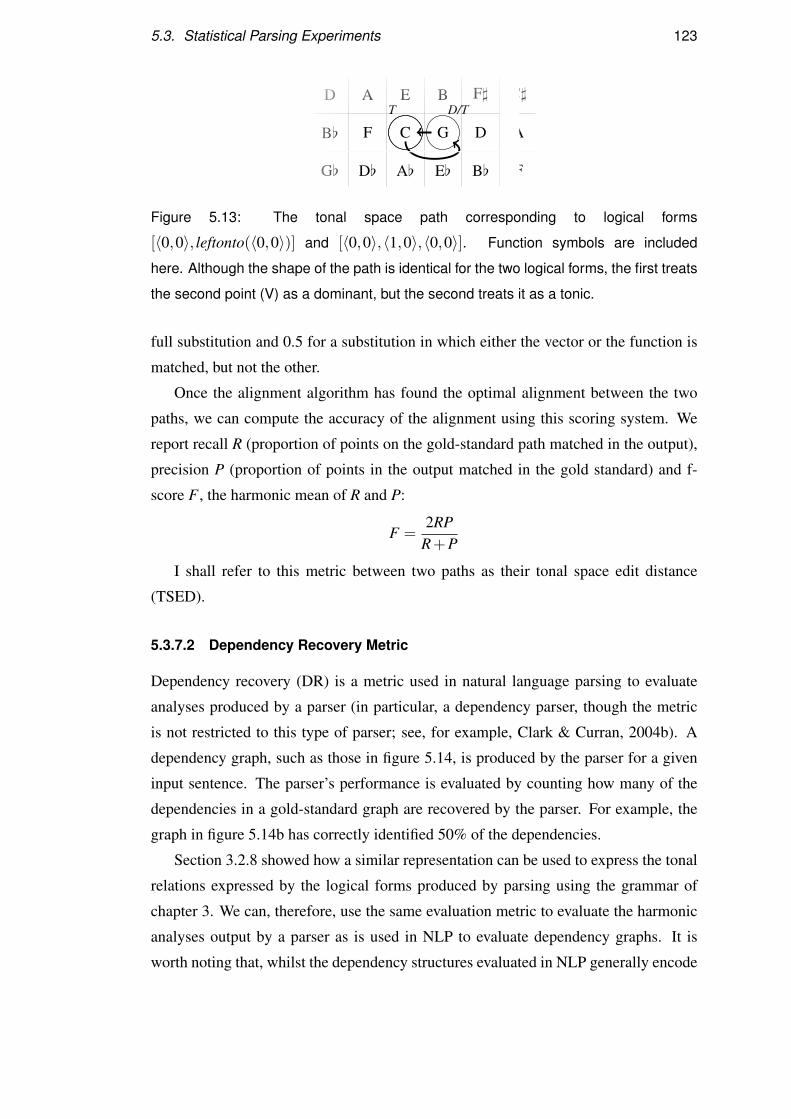
5.3. Statistical Parsing Experiments 123
G[
B[
D
D[
F
A
A[
C
E
E[
G
B
B[
D
F]
F
A
C]T D/T
Figure 5.13: The tonal space path corresponding to logical forms
[〈0,0〉, leftonto(〈0,0〉)] and [〈0,0〉,〈1,0〉,〈0,0〉]. Function symbols are included
here. Although the shape of the path is identical for the two logical forms, the first treats
the second point (V) as a dominant, but the second treats it as a tonic.
full substitution and 0.5 for a substitution in which either the vector or the function is
matched, but not the other.
Once the alignment algorithm has found the optimal alignment between the two
paths, we can compute the accuracy of the alignment using this scoring system. We
report recall R (proportion of points on the gold-standard path matched in the output),
precision P (proportion of points in the output matched in the gold standard) and f-
score F , the harmonic mean of R and P:
F =2RP
R+P
I shall refer to this metric between two paths as their tonal space edit distance
(TSED).
5.3.7.2 Dependency Recovery Metric
Dependency recovery (DR) is a metric used in natural language parsing to evaluate
analyses produced by a parser (in particular, a dependency parser, though the metric
is not restricted to this type of parser; see, for example, Clark & Curran, 2004b). A
dependency graph, such as those in figure 5.14, is produced by the parser for a given
input sentence. The parser’s performance is evaluated by counting how many of the
dependencies in a gold-standard graph are recovered by the parser. For example, the
graph in figure 5.14b has correctly identified 50% of the dependencies.
Section 3.2.8 showed how a similar representation can be used to express the tonal
relations expressed by the logical forms produced by parsing using the grammar of
chapter 3. We can, therefore, use the same evaluation metric to evaluate the harmonic
analyses output by a parser as is used in NLP to evaluate dependency graphs. It is
worth noting that, whilst the dependency structures evaluated in NLP generally encode

124 Chapter 5. Statistical Parsing of Chord Sequences
The princess kissed an unsuspecting frog
ROOT
DET SUBJ
OBJ
DET MOD
(a) A dependency graph representing the structure of a sentence.
The princess kissed an unsuspecting frog
ROOT
DET OBJ
SUBJ
ADVMOD
(b) A dependency graph such as a parser might produce for the same sentence, including
mistakes (marked by bold arcs).
Figure 5.14: Linguistic syntactic dependency graphs for a short sentence.
syntactic information, those described in section 3.2.8 fully express the information
represented in the logical forms, additionally relating it to the specific chords being
interpreted.
The experiments below are evaluated using both DR and TSED. An advantage of
the DR metric is that it is more sensitive to the parser’s performance on recovering
long-distance dependencies. A more thorough investigation of recovery of specifically
long-distance dependencies would be possible using the same technique, following
Rimell et al. (2009). In the experiments below, I report the precision, recall and f-score
(see above) of output dependencies matched against the gold standard6.
5.3.8 Results
The models are evaluated on the basis of the interpretation to which they assign highest
probability. The parser will in general produce a large number of possible interpreta-
tions where it finds any interpretation at all. These are ranked by their probability under
the probabilistic parsing model and only the most probable is used for evaluation.
6 DR is usually reported as a single percentage, since syntactic dependency graphs are typicallyconstrained to contain one dependency per word. Since the present chord dependency graphs maycontain chords not attached to any other (repeated chords, passing chords, etc.) the parser’s output andthe gold standard may have a different number of dependencies, so an f-score metric is used.

5.3. Statistical Parsing Experiments 125
Model TSED DR
P R F P R F Cov.
HMMPATH 77.44 84.87 80.98 — — — 100
PCCG 92.29 88.78 90.50 90.25 86.83 88.51 97.37
ST+PCCG 90.18 92.79 91.46 88.22 90.78 89.48 100
Table 5.2: Evaluation of each model’s prediction using 10-fold cross-validation on the
jazz corpus. Each model is scored on its TSED and DR, reporting precision (P), recall
(R), f-score (F) and coverage (Cov.), all percentages. Since ST+PCCG achieves full
coverage, no result is reported for ST+PCCG+HMMPATH. Bold results are significant
improvements over the baseline.
All models are trained and tested on the jazz corpus of chapter 4 using 10-fold
cross-validation. A timeout is imposed for individual parses of five hours of CPU
time. Table 5.2 reports the results combined from all partitions, evaluated against the
gold-standard interpretation using both TSED and DR7. Three systems are compared.
The HMMPATH model is used as a baseline. The PCCG parser is evaluated on its
own, without a supertagger and using the best supertagging model of those that were
evaluated in section 5.2, BESTNGRAM, with the AST algorithm (ST+PCCG). Since
ST+PCCG achieves full coverage, there is nothing to be gained by backing off to
HMMPATH in this experiment, in the manner suggested in section 5.3.6. Similarly,
PCCG has almost full coverage.
Differences between systems are tested for statistical significance using Dan Bikel’s
stratified shuffling test8, with 100,000 random shuffles of the results from individual
chord sequences. Results are reported as statistically significant below p = 0.05. Re-
sults significantly different from the baseline are marked in bold in table 5.2. All results
for PCCG and ST+PCCG are significantly different to the baseline, with the excep-
tion of PCCG’s recall. Evaluated by TSED, there is a significant difference between
the precision of PCCG and ST+PCCG, but not their f-scores. Evaluated by DR, the
difference in recalls is significant, but again not their f-scores.
7 Granroth-Wilding & Steedman (2012b) reported a slightly different set of results from the sameexperiments carried out with a subtly different model and different beam parameters. The experimentsreported here match more closely the experiments of Hockenmaier (2003) and use the beam settingsdetermined in section 5.3.4.4.
8 http://www.cis.upenn.edu/˜dbikel/software.html, accessed Oct 2012.
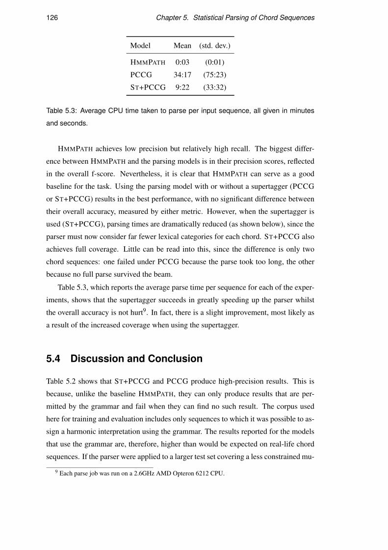
126 Chapter 5. Statistical Parsing of Chord Sequences
Model Mean (std. dev.)
HMMPATH 0:03 (0:01)
PCCG 34:17 (75:23)
ST+PCCG 9:22 (33:32)
Table 5.3: Average CPU time taken to parse per input sequence, all given in minutes
and seconds.
HMMPATH achieves low precision but relatively high recall. The biggest differ-
ence between HMMPATH and the parsing models is in their precision scores, reflected
in the overall f-score. Nevertheless, it is clear that HMMPATH can serve as a good
baseline for the task. Using the parsing model with or without a supertagger (PCCG
or ST+PCCG) results in the best performance, with no significant difference between
their overall accuracy, measured by either metric. However, when the supertagger is
used (ST+PCCG), parsing times are dramatically reduced (as shown below), since the
parser must now consider far fewer lexical categories for each chord. ST+PCCG also
achieves full coverage. Little can be read into this, since the difference is only two
chord sequences: one failed under PCCG because the parse took too long, the other
because no full parse survived the beam.
Table 5.3, which reports the average parse time per sequence for each of the exper-
iments, shows that the supertagger succeeds in greatly speeding up the parser whilst
the overall accuracy is not hurt9. In fact, there is a slight improvement, most likely as
a result of the increased coverage when using the supertagger.
5.4 Discussion and Conclusion
Table 5.2 shows that ST+PCCG and PCCG produce high-precision results. This is
because, unlike the baseline HMMPATH, they can only produce results that are per-
mitted by the grammar and fail when they can find no such result. The corpus used
here for training and evaluation includes only sequences to which it was possible to as-
sign a harmonic interpretation using the grammar. The results reported for the models
that use the grammar are, therefore, higher than would be expected on real-life chord
sequences. If the parser were applied to a larger test set covering a less constrained mu-
9 Each parse job was run on a 2.6GHz AMD Opteron 6212 CPU.

5.4. Discussion and Conclusion 127
sical domain, it would suffer from lack of coverage. The use of HMMPATH as backoff,
as discussed in section 5.3.6, would reduce the model’s precision slightly, but improve
its recall. The resulting ST+PCCG+HMMPATH model is robust in that it is guaranteed
always to produce some tonal space interpretation.
The three key conclusions to draw from these results are as follows. Firstly, they
show that HMMPATH is a reasonable model to use as a baseline for the task and to
back off to when no grammatical result can be found. Experiments on a larger data
set would without doubt suffer more severely from a lack of coverage and HMMPATH
could be used as suggested here or in a less aggressive form of backoff. Secondly, the
results show that the use of a grammar to constrain the interpretations predicted by an
HMM improves substantially over the purely short-distance information captured by
the baseline HMMPATH model. Finally, they show that the use of the AST algorithm
with a simple Markovian supertagging model succeeds in speeding up the parser by
a large factor, with no reduction in accuracy. This can be seen as using a Markovian
model to suggest some interpretations of the chords, but building the final analysis by
enforcing the structural constraints encoded in the grammar. Although this stratagem
is not essential for the present task, it is likely to be important for tasks requiring larger
models or relying on accurate parsing under time constraints, when the gain in speed
offered by supertagging will be critical.


CHAPTER 6Parsing Note-Level Performance Data
6.1 Introduction
In the previous chapters, I have considered the task of harmonic analysis from the
point of view of inferring the harmonic structure underlying a chord sequence. The
reason for approaching the analysis from this level of abstraction, rather than analysing
some representation of all the notes of a performance or an audio signal, lay rather in
the benefit of breaking a difficult analysis task down into smaller, more manageable
subtasks than in a belief that this type of chord sequence is fundamental to a description
of the harmonic analysis performed by human listeners. Indeed, certain aspects of the
grammar, such as some of the lexical entries, exist largely to deal with the fact that the
chord sequences are transcribed with practical considerations of performance in mind,
which are of no relevance to the harmonic analyser.
Nevertheless, chord sequences are a useful abstraction with which to begin the con-
struction of a harmonic analysis technique. They provide a form of the musical surface
which is already divided into units that roughly speaking correspond to the primitive
units of harmonic analysis1. The results of the experiments in the previous chapter
1 Exceptions include the consecutive repetition of a chord label with a changed type, but the sameroot and function (for example C◦7 C7) and the repetition of a chord label for the performer’s conve-nience if it spans multiple lines.
129

130 Chapter 6. Parsing Note-Level Performance Data
demonstrated that, at this level of abstraction at least, statistical parsing techniques
adapted from NLP can be used quite successfully to replicate human decisions in the
analysis of harmonic structure. There is good reason to believe that the same approach
is also applicable to harmonic analysis of less abstract input. Any technique for har-
monic analysis of the notes of a performance, for example, must segment the stream of
notes into units over which an analysis can be defined. These units, like the textual la-
bels taken as input to the parser in the previous chapter, are called chords and, although
there is not a one-to-one relationship between the two, a similar syntactic analysis will
serve to infer a structural interpretation.
An automatic analysis of performance data, note-level score data or an audio sig-
nal is an interesting application of the parsing techniques for two reasons. Firstly, it is
closer to the task that a human listener performs when listening to a piece of music. To
understand the structure of the music, they must recognize where the underlying chords
change and analyse (unconsciously) the tension-resolution relationships between these
units. Secondly, a system that can perform this task is likely to be more useful in prac-
tical applications than the chord-input parser, for example, in MIR systems (de Haas
et al., 2012).
Moving from chord sequence input to note-level information introduces many dif-
ficult problems and it is beyond the scope of this thesis to explore solutions to all of
them. For instance, I have up to now ignored the relationship between metrical and
harmonic structures, but it is clear that metrical structure plays a role for a human
listener in some aspect of harmonic analysis. The aim of this chapter is to show, by
demonstration of some simple techniques, that the approach to harmonic analysis pre-
sented in previous chapters can be extended to analysis of performance data. Some of
the added problems will be sidestepped and left for future work. Indeed, many of them
have been approached as tasks in their own right. There is a body of literature, for
example, devoted to models of metrical structure (Longuet-Higgins, 1976; Lerdahl &
Jackendoff, 1983; Cemgil et al., 2000; Raphael, 2002; Temperley, 2007; van der Weij,
2012). The approach below, therefore, makes some simplifying assumptions that per-
mit an initial approach to the task. The models described in this chapter operate on
performance data represented at the level of keyboard notes in a symbolic, electronic
format. However, the same ideas could be used to extend the system to analysis of
audio data, with the result of introducing extra noise into the models.
Some of the models and experiments described in this chapter have previously been
presented by Granroth-Wilding & Steedman (2012a).

6.2. Data Representation: MIDI 131
6.2 Data Representation: MIDI
MIDI (Musical Instrument Digital Interface, MIDI Manufacturers Association, 1996)
is a digital representation of the notes of a musical performance. It was originally de-
signed for sending instructions between electronic musical instruments. The instruc-
tions, or events, can be stored in MIDI files in the form of a stream of events, each
associated with a time. It can be produced by recording events as they are played on an
instrument or by generating a list of events directly from an electronic representation
of a score. The format of a MIDI file is standardized and included in the specification
of the MIDI protocol.
The events of a MIDI stream may include a wide variety of information besides the
notes played: the instrument type, changes in dynamics, even changes to the tuning of
the instrument. At its simplest, MIDI data is just a stream of note onset and note offset
events, specifying times when played notes begin and end.
MIDI provides a useful symbolic representation of musical performances in which
to take input to a harmonic analysis system. It has the benefit of being a widely ac-
cepted data format in which recorded and score-generated performances are readily
available.
6.3 Adding MIDI to the Jazz Corpus
The corpus described in chapter 4 contains chord sequences annotated with grammati-
cal analyses, used as training and testing data for supertagging and parsing models. In
order to develop note-level models of performances, a similar dataset made up of MIDI
files is required. The laborious process of annotating the MIDI data with grammatical
analyses can be avoided by using MIDI performance data for the same songs as are
already in the corpus.
MIDI files are readily available on the web, but they are of widely varying qual-
ity and few reliable sources of high-quality files exist. I have extended the jazz chord
corpus with MIDI files by first automatically collecting a large number of MIDI files
from several websites that have a good coverage of the domain and then filtering them.
The collection process searched several specialized MIDI search engines, download-
ing files for all results. The retrieved set was filtered both automatically, to remove
duplicates, and manually, to remove poor quality files or performances of the wrong
song. The automatic filter compared the files pairwise to identify exact duplicates and
132 Chapter 6. Parsing Note-Level Performance Data
duplicates with only small modifications (it is common to redistribute files, for exam-
ple, with just the instrumentation changed). The resulting set contained roughly 350
files.
The models described below require some additional information about the MIDI
files. They assume that the performance is metronomic: that is, that the performer
has played with a metronome (or drum backing) during the recording and that the
metronome beat can be recovered from the MIDI data. Fortunately, this assumption
holds for many of the MIDI files collected from the web. The models require further
that they know where the barlines occur relative to the metronome beat – in other
words, that they know the time signature. If a MIDI file is metronomic, it need only be
annotated with the length of a bar expressed in terms of metronome beats and the start
time relative to the start of the MIDI file of the first bar. It is then trivial to divide the
whole file into metrical units, such as bars.
Using the evaluation metrics described below in section 6.4.4, a parser that takes
input in the form of a MIDI file can be evaluated against the harmonic analysis of the
chord sequence for the same song already in the corpus. Jazz performances typically
involve playing the song’s melody once through (the head) and then repeating the
chord sequence many times with improvised melodies. In order for the analysis of the
MIDI data to be comparable to the gold-standard analysis, either the parser must detect
this repetition and produce an analysis of the repeated chord sequence or the input
must have been cut so that it includes only the head. The former approach is beyond
the scope of this project, so MIDI inputs cut down to just the head are evaluated. The
experiments below use a set of the MIDI files which have been cut to contain only the
head and annotated with the metrical information. The set consists of 41 MIDI files.
6.4 Pipeline Approach
6.4.1 Chord Recognizer as a Frontend to the Supertagger
A simple first step towards a system for parsing MIDI input is to apply a strict pipeline
approach that incorporates the chord-input parser of the previous chapter. First, a
model is used to choose a single sequence of chord labels from the MIDI input. I
shall refer to this component of the system as the chord recognizer. The parser and
supertagger can then be used without modification to analyse the chord sequence as
before.

6.4. Pipeline Approach 133
There is good reason to expect such a naive approach to give poor results. The
interpretations of the chord-based parser are severely constrained by the input chord
sequence. In some cases, it is unable to find any analysis of a particular input. There-
fore, if the chord recognizer does a bad job of segmenting and labelling the MIDI data,
the parser will be forced to produce a poor analysis, or no analysis at all. To ensure
that the chord sequence supports a meaningful analysis, the chord recognizer would
need to be able to take into consideration aspects of the harmonic structure like key
(with potential modulation) and cadence structure – exactly the structures the parser is
designed to capture. What is more, it is not clear that the sort of chord labels that are
designed primarily with a performer’s interests in mind, are a useful intermediate level
of representation between the MIDI data and the analysis. Despite these objections,
this approach is an obvious starting point for the task of parsing from MIDI input, since
it is a straightforward extension to the models already presented.
The task of automatic chord recognition2 has been extensively studied, but has
most often been tackled as the task of inferring chord labels from an audio signal
(among others, Sheh & Ellis, 2003; Ni et al., 2011; Harte & Sandler, 2005). Rather
than devising a new model for MIDI-based chord recognition, it is possible to adapt
a recent high-performing, audio-based model to the task. Ni et al. (2011) present an
HMM-based model for audio chord recognition. The MIDI model used here is based
on this and substitutes the emission distribution of their HMM, defined over frequency
bands corresponding to pitch classes, with a similar distribution over pitch classes as
represented in the MIDI data. Each state encodes three pieces of information: the
current key Ki, the root of the current chord CRi and the type of the current chord CT i.
The original model also encoded the bass note, linked by the emission distribution to
a low frequency range. The present model does not include this, since it is not a trivial
task to decide which notes in the MIDI data should be considered bass notes, and
because including it increases the number of model parameters that must be trained,
which is likely to have a negative effect when training on a small dataset.
The notion of tonality captured by the present model as K is in fact more local than
what would usually be meant by key. It corresponds to the resolutions of cadences that
are expressed in the formal language of chapter 3, which include brief tonicizations as
well as longer-term modulations to a new key.
2 I use the term chord recognition to refer to the extraction of chord labels, of the sort taken as inputto the system of the previous chapter, from performance data. The harmonic analysis performed bythe parser could also be thought of as a sort of chord recognition, explicitly representing the structuredrelationships between chords. There exists a variety of forms of analysis between the two (see, forexample, Raphael & Stoddard, 2004).

134 Chapter 6. Parsing Note-Level Performance Data
The transition and emission distributions are constrained in certain ways. The tran-
sition distribution is defined as:
Ptr-cr(Ki, CRi, CT i | Ki−1, CRi−1, CT i−1) =
Ptr-cr-rt(δ(CRi,Ki), CT i | δ(CRi−1,Ki−1), CT i−1)×Ptr-cr-key(δ(Ki,Ki−1))
The chord root is taken relative to the key (using δ, as defined in section 5.2.2.1)
and the chord root and type are conditioned only on the previous chord root and type.
Key transitions are modelled independently and are taken relative to the first key.
The emission distribution treats the MIDI notes as a bag of notes: each is emitted
independently, conditioned on the chord root and type of the state, but ignoring the
key. The distribution is defined as:
Pem-cr(n | CRi, CT i) = ∏n∈n
Pem-cr-nt(δ(n,CRi) | CT i)
The pitches of the notes n are taken relative to the current chord’s root and the
emission distribution for each note is conditioned only on the chord type.
An HMM can be trained in an unsupervised fashion – using data without annotation
of the correct state labels – with the EM algorithm (Rabiner, 1989). The parameters of
the transition and emission distributions are initialized crudely, potentially by super-
vised training on a small dataset, and the model’s parameters are retrained on a large
unlabelled dataset by an iterative algorithm that is guaranteed to increase the likelihood
with which the model predicts the training data. In the present case, the transition dis-
tribution is initialized by maximum likelihood estimation over the chord sequences in
the jazz chord corpus, with chords repeated in proportion to their length. The neces-
sary key information is extracted from the annotated harmonic analyses. The emission
distribution is initialized by assigning an equal, arbitrarilly chosen high probability to
each of the notes in the chord (for example 0, 4, 7 and 11 for the chord type CM7) and
a low probability to any other notes. The model is then retrained using EM over the
entire set of MIDI files.
The HMM can produce a single best chord sequence for a MIDI file using the
Viterbi algorithm (Viterbi, 1967) to find the most probable sequence of states and ex-
tracting chord labels from this (CR and CT). Repeated states are merged into a single
chord label, since self transitions signify a continuation of the same chord.
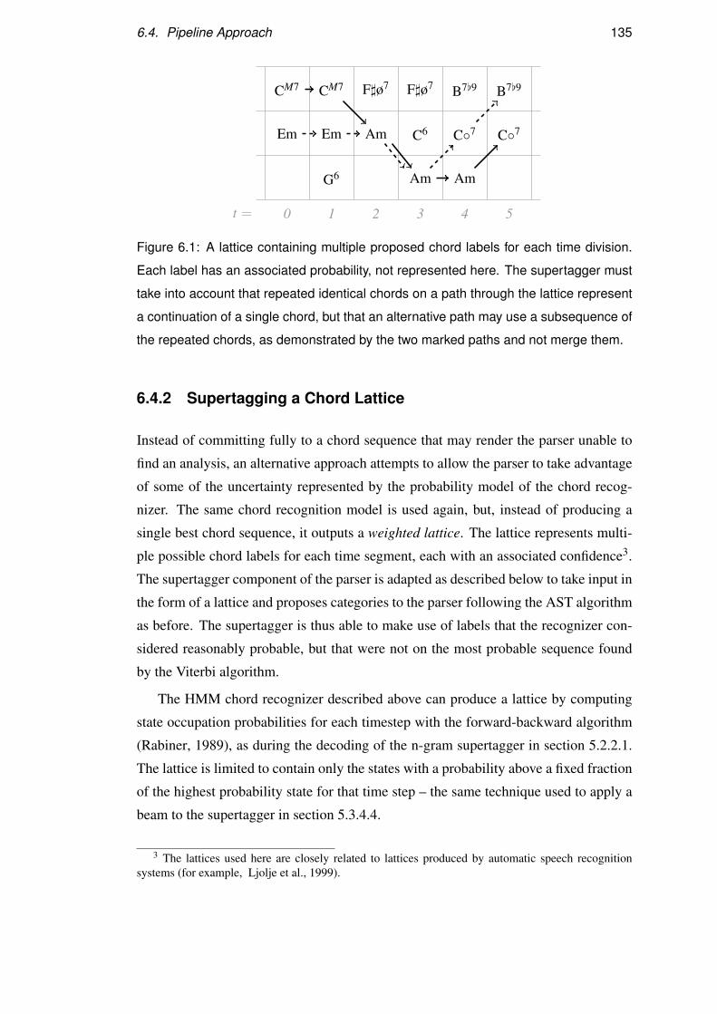
6.4. Pipeline Approach 135
CM7
Em
CM7
Em
G6
F]ø7
Am
F]ø7
C6
Am
B7[9
C◦7
Am
B7[9
C◦7
t = 0 1 2 3 4 5
Figure 6.1: A lattice containing multiple proposed chord labels for each time division.
Each label has an associated probability, not represented here. The supertagger must
take into account that repeated identical chords on a path through the lattice represent
a continuation of a single chord, but that an alternative path may use a subsequence of
the repeated chords, as demonstrated by the two marked paths and not merge them.
6.4.2 Supertagging a Chord Lattice
Instead of committing fully to a chord sequence that may render the parser unable to
find an analysis, an alternative approach attempts to allow the parser to take advantage
of some of the uncertainty represented by the probability model of the chord recog-
nizer. The same chord recognition model is used again, but, instead of producing a
single best chord sequence, it outputs a weighted lattice. The lattice represents multi-
ple possible chord labels for each time segment, each with an associated confidence3.
The supertagger component of the parser is adapted as described below to take input in
the form of a lattice and proposes categories to the parser following the AST algorithm
as before. The supertagger is thus able to make use of labels that the recognizer con-
sidered reasonably probable, but that were not on the most probable sequence found
by the Viterbi algorithm.
The HMM chord recognizer described above can produce a lattice by computing
state occupation probabilities for each timestep with the forward-backward algorithm
(Rabiner, 1989), as during the decoding of the n-gram supertagger in section 5.2.2.1.
The lattice is limited to contain only the states with a probability above a fixed fraction
of the highest probability state for that time step – the same technique used to apply a
beam to the supertagger in section 5.3.4.4.
3 The lattices used here are closely related to lattices produced by automatic speech recognitionsystems (for example, Ljolje et al., 1999).

136 Chapter 6. Parsing Note-Level Performance Data
Figure 6.1 shows an example of a lattice stretching over several timesteps. When
a single chord sequence was decoded from the chord recognizer, repeated chords were
treated as a continuation of the same chord. The lattice-based supertagger must do the
same for paths through the lattice that result in repeated chord labels, but still allow
for all possible paths through the lattice. For example, two possible paths are marked
on figure 6.1. The solid path results in the chord sequence CM7 Am C◦7, the dotted
path Em Am C◦7. However, the solid path remains on Am for three timesteps, but
the dotted one only two. Furthermore, two alternative chords labels may result in the
same category. For example, in timestep 4 the lexicon will permit the same category
to be assigned to B7[9 and C◦7 (by the Dom and Dim-III schemata respectively). One
possible sequence of categories resulting from the dotted path, therefore, involves the
continuation of this category from timestep 4 to 5. To capture this, the supertagger
must handle the continuation of chords after proposing categories, rather than at the
level of the chord lattice.
The n-gram supertagging model of chapter 5 can be adapted to assign categories
to a chord lattice, instead of a single chord sequence, by the following simple modifi-
cation. In section 5.2.2.1, the transition and emission distributions of the supertagging
model were defined as:
Ptr-st(Schi,SRi |Schi−n+1,...,i−1,SRi−n+1,...,i−1) =
Ptr-sch(Schi |Schi−n+1,...,i−1)×Ptr-rt(δ(SRi,SRi−1)|Schi)
Pem-st(CT i,CRi |Schi,SRi) =
{Pem-tp(CT i |Schi) if CRi = SRi
0 o/w
Each state represents a schema Schi and a root SRi. Emissions are treated as a chord
type CT i and root CRi. The emission probability is 0 wherever the state’s root does
not match the chord’s root. A supertagger for a chord lattice can be constructed by
modifying the emission distribution so that it emits a set of chords (types and roots).
The emission distribution then becomes:
Pem-lat(CT0i ,CR0
i , . . . ,CTCi ,CRC
i |Schi,SRi) =
∑c=0,...,C
Pem-st(CTci ,CRc
i |Schi,SRi)×Plat(CRci ,CTc
i |M)
Plat(CRci ,CTc
i |M), the probability of a chord label with the MIDI input data M, is
obtained from the chord recognizer’s state occupation probabilities, computed by the
forward-backward algorithm. This has the effect of weighting the probability of each
chord by the confidence that the chord recognizer had in the chord label, resulting in
a weighted average of the chords in the lattice at each timestep. Note that the matrix
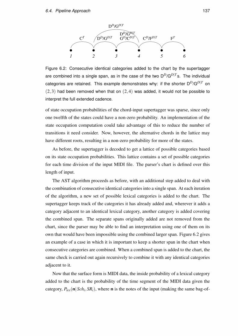
6.4. Pipeline Approach 137
1 2 3 4 5 6
CT DD/GD|TDD/GD|T
GD/CD|T CD/FD|T FT
DD/GD|T
Figure 6.2: Consecutive identical categories added to the chart by the supertagger
are combined into a single span, as in the case of the two DD/GD|T s. The individual
categories are retained. This example demonstrates why: if the shorter DD/GD|T on
(2,3) had been removed when that on (2,4) was added, it would not be possible to
interpret the full extended cadence.
of state occupation probabilities of the chord-input supertagger was sparse, since only
one twelfth of the states could have a non-zero probability. An implementation of the
state occupation computation could take advantage of this to reduce the number of
transitions it need consider. Now, however, the alternative chords in the lattice may
have different roots, resulting in a non-zero probability for more of the states.
As before, the supertagger is decoded to get a lattice of possible categories based
on its state occupation probabilities. This lattice contains a set of possible categories
for each time division of the input MIDI file. The parser’s chart is defined over this
length of input.
The AST algorithm proceeds as before, with an additional step added to deal with
the combination of consecutive identical categories into a single span. At each iteration
of the algorithm, a new set of possible lexical categories is added to the chart. The
supertagger keeps track of the categories it has already added and, wherever it adds a
category adjacent to an identical lexical category, another category is added covering
the combined span. The separate spans originally added are not removed from the
chart, since the parser may be able to find an interpretation using one of them on its
own that would have been impossible using the combined larger span. Figure 6.2 gives
an example of a case in which it is important to keep a shorter span in the chart when
consecutive categories are combined. When a combined span is added to the chart, the
same check is carried out again recursively to combine it with any identical categories
adjacent to it.
Now that the surface form is MIDI data, the inside probability of a lexical category
added to the chart is the probability of the time segment of the MIDI data given the
category, Plex(n|Schi,SRi), where n is the notes of the input (making the same bag-of-

138 Chapter 6. Parsing Note-Level Performance Data
2 3 4
DD/GD|TDD/GD|T
GD/CD|T
DD/GD|T
DD/CD|T
Figure 6.3: Part of the chart shown in figure 6.2. This chart also includes the category
added to the span (2,4) by composition of DD/GD|T and GD/CD|T .
notes assumption as the chord recognizer). This can be estimated using a combination
of the emission distributions of the supertagger and the chord recognizer:
Plex(n|Schi,SRi) = ∑c=0,...,C
Pem-st(CRci ,CTc
i |Schi,SRi)×Pem-cr(n|CRci ,CTc
i )
For each chord in the lattice, the supertagger’s emission distribution gives the probabil-
ity of that chord label conditioned on the state. This is multiplied with the probability
from the chord recognizer’s emission probability: the probability of the observed MIDI
notes conditioned on the chord label. The probability is summed over the chords in the
lattice.
Inside probabilities must also be associated with categories resulting from combi-
nations of adjacent identical categories. Consider again the categories in figure 6.2,
repeated in part in figure 6.3. The DD/GD|T categories on spans (2,3) and (3,4) have
inside probabilities computed as above. They are combined to produce the same cate-
gory for the span (2,4) and this too requires an inside probability. An obvious strategy
would be to give it the product of the probabilities of the combined categories. How-
ever, this gives too high a probability to the category when compared to a category on
the same span produced by rule applications – DD/CD|T in the example, which was
produced by composition of DD/GD|T with GD/CD|T . The inside probability of this
category has been computed as the product of not only the two lexical categories, but
also the probability of their combination in a rule application (see the derivation model
of section 5.3.4). The more consecutive identical categories are combined, the greater
an advantage these will have over categories on the same span produced by rule appli-
cations.
The model penalizes inside probabilities of categories produced by combining
identical rules proportionally to the number of nodes that there would have been in
6.4. Pipeline Approach 139
a derivation tree that produced a category on the same span by binary rule applica-
tions. This number is the nth triangular number, where n is the width of the span. The
nth triangular number is given by the binomial coefficient(n+1
2
). The penalized inside
probability for a span with lexical probabilities L is computed as:
(∏p∈L
p)(|L|+1
2 )
In the example in figure 6.3, the span (2,4) requires the 2nd triangular number,
3. The penalized probability is the product of the two lexical probabilities raised to
the power of 3. This strategy has the effect of scaling the probabilities of combined
categories to approximately the same order of magnitude as others in the same cell of
the chart.
6.4.3 HMM Baseline
The HMM baseline model HMMPATH, described in section 5.3.5, can be adapted to
assign a tonal space interpretation to MIDI data in the same way as the supertagging
model was above. As with the supertagger, experiments are run under two scenarios:
pipeline, in which the input to HMMPATH is the single best chord sequence given
by Viterbi decoding of the chord recognizer, and lattice, in which HMMPATH takes
account of multiple weighted chord labels from the chord recognizer.
The emission distribution of HMMPATH was defined in section 5.3.5 as:
Pem-hp(CT i, CRi | subi, blocki, funi) =
Pem-hp-root(δ(CRi, subi) | funi)×Pem-hp-type(CT i | δ(CRi, subi), funi)
In the lattice case, the emission distribution of HMMPATH is adapted, as the n-gram
supertagging model’s was, to allow it to take account of all the suggested chord labels
and the chord recognizer’s confidence in each. The emission probabilities are averaged
over each of the chords in the lattice, weighted by the chord recognizer’s confidence in
the chord label:
Pem-hp-lat(CT0i , CR0
i , . . . , CTCi , CRC
i | subi, blocki, funi) =
∑c=i,...,C
Pem-hp(CTci , CRc
i | subi, blocki, funi)×P(CTci , CRc
i | O)
Once again, the probability P(CTci , CRc
i | O) is obtained from the chord recog-
nizer’s state occupation matrix. The decoding process is identical to the use of the
model for chord sequence interpretation.

140 Chapter 6. Parsing Note-Level Performance Data
6.4.4 Evaluation
In chapter 5, the chord-input parser was evaluated using two metrics: TSED and DR.
The midi-input parser can be evaluated using both of these metrics, though the lat-
ter requires some modification. The analysis produced by the parser is evaluated by
comparing it to the gold-standard analysis of the same song from the corpus. Since
the analysis in the corpus was defined over the chord sequence and not the specific
performance, it is possible that it is not quite the same as a gold-standard analysis
defined over the performance data would be: the performer may, for example, have
played from a slightly different chord sequence or elaborated or simplified the har-
mony. However, most such changes will not have a great effect on the analysis and
some, like chord substitution, will not affect it at all. It is reasonable to assume that
the gold-standard chord sequence analysis is at least a close approximation to a gold
standard for the performance data.
The TSED metric over paths through the tonal space can be used without modifi-
cation to evaluate the output of a MIDI-input parser, since it can be used to compare
any two analyses, regardless of the input that they analyse. The DR metric, however,
is not directly applicable.
6.4.4.1 Evaluating DR without Token Alignment
Because the parser incorporates the task of chord segmentation, it is not possible to
evaluate its DR directly against the gold standard. This same problem exists for eval-
uation of any system that performs segmentation of its input as a part of the analy-
sis process. Examples from NLP include a parser that incorporates automatic speech
recognition to provide an analysis of spoken input; and a parser for languages that re-
quire morphological segmentation (Tsarfaty et al., 2012). The MIDI parsing task, then,
requires an evaluation metric that can measure the similarity between the structure and
arc labels of two dependency graphs without knowing beforehand the alignment be-
tween their nodes.
One suitable metric can be thought of as an optimized version of the DR metric.
It first finds the alignment between the nodes of the parser’s dependency graph and
the gold-standard graph that maximizes the number of dependencies recovered and
then uses that to compute the precision and recall of DR. Additionally, for the present
task, the key of the MIDI-encoded performance is unknown and may not necessarily
be the same as the key of the sequence in the corpus. The metric, therefore, computes

6.4. Pipeline Approach 141
E7 E[7 A[7 G7 C
leftontoleftontoleftontoleftonto
〈0,0〉
leftonto
〈0,0〉
leftontoleftonto
〈0,2〉
Figure 6.4: Correct and maximal alignment between a gold-standard dependency graph
sequence and a system’s output for MIDI data of a performance. The system has
misinterpreted the tritone substitution A[7 as a tonic resolution. It has correctly identified
the rest of the extended dominants (leftonto) and the final tonic resolution, which the
metric gives it credit for.
the optimal alignment for each of the 12 possible transpositions of the analyses (that
is, transpositions of the tonic labels) and chooses the one which maximizes DR. The
resulting metric is called optimized dependency recovery (ODR).
The reason for finding the optimal alignment is that, given that the true correspon-
dence between the chord labels and times in the unsegmented input is unknown, the
metric must give the system credit for any parts of the dependency graph that can be
matched. Such a metric can be expected to overestimate the performance of the system
in some cases, as shown below, but will never underestimate it.
Figure 6.4 shows an alignment between two analyses of an extended cadence, the
gold-standard analysis on top and an analysis such as might be output by a MIDI parser
underneath. Chord symbols are shown only for the gold-standard analysis, since the
nodes of the graph of the parser’s output correspond to segments of MIDI data. Despite
this, it is possible to see at a glance the mistake the parser has made: it has treated the
third chord as a tonic resolution of the preceding dominant. Using the optimal node
alignment to evaluate ODR gives the parser credit not only for the last dominant and
tonic, but also for the first two dominant relations, which it correctly identified.
Figure 6.5 shows two possible alignments between a gold-standard dependency
graph for a chord sequence and one that might be output for a system processing a
MIDI file for the same song. The correct alignment of the MIDI data with the chord
sequence is unknown. The system has segmented the Dm7 chord too finely and inter-
preted it as several extended dominants (the first three leftontos). It has treated the A7,
D7 and G7 as tonics. Figure 6.5a, therefore, shows the correct alignment between the
nodes of the graphs. However, since information about the chords played in the MIDI
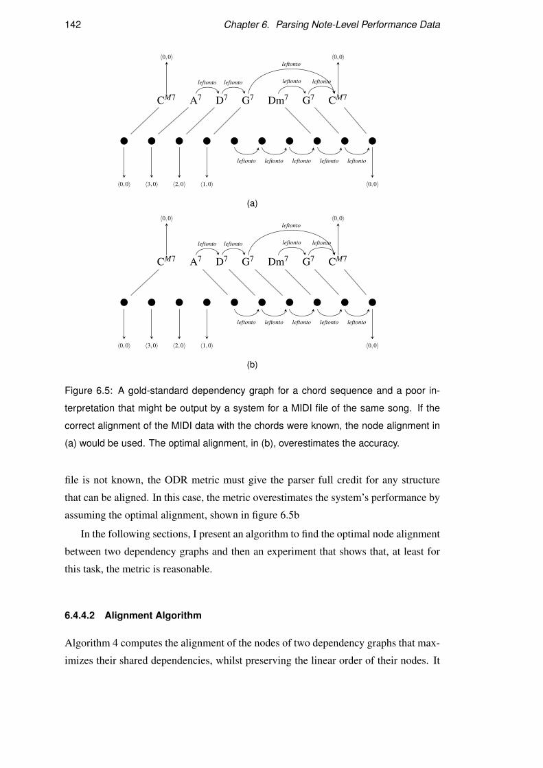
142 Chapter 6. Parsing Note-Level Performance Data
CM7 A7 D7 G7 Dm7 G7 CM7
〈0,0〉
leftonto leftonto
leftonto
leftonto leftonto
〈0,0〉
〈0,0〉 〈3,0〉 〈2,0〉 〈1,0〉
leftonto leftonto leftonto leftonto leftonto
〈0,0〉
(a)
CM7 A7 D7 G7 Dm7 G7 CM7
〈0,0〉
leftonto leftonto
leftonto
leftonto leftonto
〈0,0〉
〈0,0〉 〈3,0〉 〈2,0〉 〈1,0〉
leftonto leftonto leftonto leftonto leftonto
〈0,0〉
(b)
Figure 6.5: A gold-standard dependency graph for a chord sequence and a poor in-
terpretation that might be output by a system for a MIDI file of the same song. If the
correct alignment of the MIDI data with the chords were known, the node alignment in
(a) would be used. The optimal alignment, in (b), overestimates the accuracy.
file is not known, the ODR metric must give the parser full credit for any structure
that can be aligned. In this case, the metric overestimates the system’s performance by
assuming the optimal alignment, shown in figure 6.5b
In the following sections, I present an algorithm to find the optimal node alignment
between two dependency graphs and then an experiment that shows that, at least for
this task, the metric is reasonable.
6.4.4.2 Alignment Algorithm
Algorithm 4 computes the alignment of the nodes of two dependency graphs that max-
imizes their shared dependencies, whilst preserving the linear order of their nodes. It

6.4. Pipeline Approach 143
C E7 A7 Dm7 G7 Dm7 D[7 C
〈0,0〉
leftonto leftonto leftonto
leftonto
leftonto leftonto
〈0,0〉
(a)
〈0,0〉
leftontoleftonto
leftonto
leftonto
leftonto leftonto leftonto
〈0,0〉
(b)
Figure 6.6: Alignment of a subsequence of nodes. The algorithm must keep track of
multiple alignments of the current subsequence (grey box), since its score depends on
later node alignment. The alignment shown contains three matched dependencies, but
may permit one more (thick lines) if the final nodes of (a) and (b) are aligned.
is based on Wagner & Fischer’s (1974) algorithm, which computes the Levenshtein
distance, or edit distance, between two strings by finding a minimal sequence of edits
(deletions, insertions, substitutions) that transforms one string into the other.
The edit distance algorithm uses dynamic programming to compute the optimal
alignment efficiently. It uses the observation that the optimal alignment of the first i
characters of a string S0, written S0〈1 : i〉, with the first j characters of S1, S1〈1 : j〉,can be found by the following procedure. The optimal alignments are found between
S0〈1 : i−1〉with S1〈1 : j〉, S0〈1 : i〉with S1〈1 : j−1〉 and S0〈1 : i−1〉with S1〈1 : j−1〉.Then the alignment is picked that has the smallest cost after the insertion of S1( j), the
deletion of S0(i) or the substitution of S1( j) for S0(i), respectively. After each choice,
only the optimal alignment and its score need be stored, since any alignment including
a non-optimal alignment of subsequences could be improved by using the optimal one.
A similar procedure solves the present node alignment problem. In this case, we
cannot throw away all but the optimal alignment of subsequences of nodes, since those
choices could affect not only the score of the sub-alignment, but also the score available
to later alignments, since it may align one end of a dependency whose other end falls
outside the subsequence. In the example in figure 6.6, the choice of whether to use the
particular alignment in the grey box affects not just the score of the subsequence itself,
but the score of aligning the final nodes, due to the dependencies passing the right edge
of the box (marked by thick lines).

144 Chapter 6. Parsing Note-Level Performance Data
The basic outline of the Wagner-Fischer algorithm can be used to compute all pos-
sible alignments for every pair of subsequences. This gives us a strategy for exploring
every possible node alignment – an approach with exponential complexity, since the
number of possible alignments is (m+n)!m!n! , where m and n are the numbers of nodes in
the two dependency graphs. However, it need not explore every possibility: although
multiple possible subsequence alignments must be kept, we can throw away many of
the sub-alignments on the basis that they can never form a part of the overall optimal
alignment.
For any subsequence alignment L0, such as the grey box in figure 6.6, the subse-
quence contributes to the overall score at least the number of dependencies already
matched, matchedL0 (three, in this case). It could also permit the matching of candL0
further dependencies – those crossing the right border (one here). If an alternative
alignment L1 of the same subsequences has matchedL1 and candL1 such that
matchedL1 +candL1 ≤ matchedL0 , it can be discarded: any full alignment containing
the alignment L1 would achieve at least the same score using L0 instead, without plac-
ing any constraints on the alignment of the nodes that follow.
The full algorithm is shown in algorithm 4. For each possible alignment a↔ b
between the ath node of A and the bth node of B, the table D[a,b] stores a set of pairs
(matched,cand), each representing a particular alignment of the nodes up to Aa and Bb
that ends with Aa aligned with Bb. matched stores the number of dependencies matched
within the aligned subsequences and cand a bag of pairs (i, j) representing future node
alignments that would result in a matched dependency4. T , as in the edit distance
algorithm, stores a trace of the last operation (deletion, insertion or alignment) that led
to each alignment represented in D. In addition to pointing to the relevant cell of D (up,
left or diagonally), it must also specify the index of the relevant alignment pair within
the cell. The tables are filled in a similar way to the edit distance algorithm. Lines 15
and 16 create a list of all the node pairs which, if aligned, will cause dependencies
from a and b to match. The first term (line 15) collects pairs of nodes which have
similarly labelled arcs pointing to the pair currently being aligned. The second (line 16)
collects pairs with similarly labelled arcs from the current pair. Lines 23–25 prune
out of D[a,b] any alignment candidates whose maximum possible score, including
dependencies that might be matched by later alignments, (matchedk+|candk |) is less
than the score matchedmaxk already reached by another alignment.
4 Note that cand could contain the same node pair multiple times, since multiple dependencies mayattach to the same node.

6.4. Pipeline Approach 145
Algorithm 4: nodealign(A,B) – optimal node alignment algorithm
1 roots←{(a,b) | ∀a,b.∃ lab .((a lab→ ROOT) ∈ A∧ (b lab→ ROOT) ∈ B)}2 for a← 0, |A|−1 do D[a,0]←{(0, /0)}3 for b← 1, |B|−1 do D[0,b]←{(0, /0)}4 for a← 1, |A|−1 do
5 for b← 1, |B|−1 do
6 D[a,b], T [a,b]← /0
7 for (matchedk,candk) ∈ D[a−1,b] do
8 cand′← remove all (a,x) from candk
9 add (matchedk,cand′) to D[a,b]
10 add ( ,k) to T [a,b]
11 for (matchedk,candk) ∈ D[a,b−1] do
12 cand′← remove all (x,b) from candk
13 add (matchedk,cand′) to D[a,b]
14 add ( ,k) to T [a,b]
15 newdeps←{(x,x′) | ∃a,b, lab .(a lab→ x) ∈ A ∧ (b lab→ x′) ∈ B ∧ x < a ∧ x′ < b}
16 ] {(x,x′) | ∃a,b, lab .(x lab→ a) ∈ A ∧ (x′ lab→ b) ∈ B ∧ x < a ∧ x′ < b}17 for (matchedk,candk) ∈ D[a−1,b−1] do
18 m← count (a,b) in candk
19 if (a,b) ∈ roots then m← m+1
20 cand′← remove all (a,b) from cand
21 add (matchedk+m,candk]newdeps) to D[a,b]
22 add ( ,k) to T [a,b]
23 (matchedmaxk,candmaxk)←maxmatched(D[a,b])
24 remove all (matchedk,candk) from D[a,b] where
matchedk+|candk | ≤ matchedmaxk and k 6= maxk
25 remove corresponding entries from T

146 Chapter 6. Parsing Note-Level Performance Data
Algorithm 5: trace(T,A,B) – optimal alignment trace retrieval
1 k← 0
2 a← |A|−1
3 b← |B|−1
4 while a > 0 ∧ b > 0 do5 (dir,k)← T [a,b]k6 if dir = then b← b−1
7 else if dir = then b← b−1
8 else if dir = then9 print(a, b)
10 a← a−1
11 b← b−1
The number of dependencies in the maximal alignment can be retrieved at the end
from the last cell, D[|nodes(A)| − 1, |nodes(B)| − 1]. This cell contains exactly one
(matched,cand) pair, where matched is the number of dependencies matched, since
cand must be empty. The trace of an alignment that gave the maximal matching can be
retrieved from T by algorithm 5, as in the edit distance algorithm. The algorithm out-
puts each pair of nodes (a,b) that was aligned in the alignment with maximal matched
dependencies.
6.4.4.3 Faithfulness of the ODR Metric
If the ODR metric is applied to system output for which a correct segment alignment
is known, it will in general overestimate the true DR score. Before using the metric to
evaluate the output of a MIDI parser, for which there is no correct alignment available,
it is helpful to get an idea of how much the results benefit from the optimization of the
segment alignment.
Table 6.1 reports the results of the chord-input parsing experiment, first seen in sec-
tion 5.3.8, evaluated both by DR and ODR. The results show that ODR overestimates
the performance of the parser by only a couple of percentage points on each measure.
One notable difference between ODR and DR is that ODR becomes less mean-
ingful a measure by which to compare two systems the lower their results are. In a
dependency graph differing only slightly from the gold standard, a misalignment of a
node that results in an extra recovered dependency will usually result in the loss of at

6.4. Pipeline Approach 147
P R F
ST+PCCG (DR) 88.22 90.78 89.48
ST+PCCG (ODR) 89.65 92.25 90.93
Table 6.1: Accuracy of the chord sequence parser measured using DR as before and
ODR, which must be used to evaluate the output of a MIDI-input parser. Each is evalu-
ated by precision (P), recall (R) and f-score (F), all percentages.
least one other dependency. As the similarity between the two graphs gets lower, there
is more to be gained by misalignments, so ODR can be expected be more generous to
very low scoring systems.
6.4.5 Results
The results of the MIDI parsing experiments are reported in table 6.2. CR+HMMPATH
is the extension of the HMMPATH chord baseline to MIDI using the chord recognizer
under pipeline and lattice scenarios. Likewise, CR+ST+PCCG is the extension of
ST+PCCG with the chord recognizer.
Certain points should be born in mind when looking at these results. ST+PCCG
results are included in this table (repeated from table 5.2): these are not a baseline
for these experiments, but rather a ceiling, since they are results from an easier task. It
would be surprising if a system processing MIDI input as an extension of the statistical
parsing of ST+PCCG achieved results even close to these. Furthermore, the evaluation
of the system is a little unsatisfactory. It is based on the assumption that a correct anal-
ysis of the relationships between chords in a MIDI-encoded performance will produce
an identical structure to the gold-standard annotated dependency graph for the chord
sequence of the same song. This might not hold in all cases, for reasons mentioned
above. More problematic, however, is that the chord sequence used by the performer
might not match that in the corpus: it is common to find many different transcriptions
and arrangements of any particular song. In this case, a perfect replication of the chord
dependencies according to the annotation procedure described in chapter 4 would not
score 100% when compared to the gold-standard annotations. Nevertheless, we can
expect that the score would not be far from 100%, since the variations between chord
sequences will typically preserve much of the dependency structure.
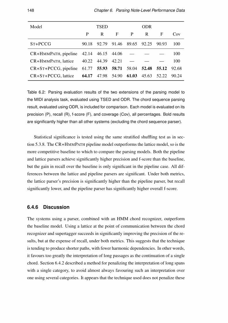
148 Chapter 6. Parsing Note-Level Performance Data
Model TSED ODR
P R F P R F Cov
ST+PCCG 90.18 92.79 91.46 89.65 92.25 90.93 100
CR+HMMPATH, pipeline 42.14 46.15 44.06 — — — 100
CR+HMMPATH, lattice 40.22 44.39 42.21 — — — 100
CR+ST+PCCG, pipeline 61.77 55.93 58.71 58.04 52.48 55.12 92.68
CR+ST+PCCG, lattice 64.17 47.98 54.90 61.03 45.63 52.22 90.24
Table 6.2: Parsing evaluation results of the two extensions of the parsing model to
the MIDI analysis task, evaluated using TSED and ODR. The chord sequence parsing
result, evaluated using ODR, is included for comparison. Each model is evaluated on its
precision (P), recall (R), f-score (F), and coverage (Cov), all percentages. Bold results
are significantly higher than all other systems (excluding the chord sequence parser).
Statistical significance is tested using the same stratified shuffling test as in sec-
tion 5.3.8. The CR+HMMPATH pipeline model outperforms the lattice model, so is the
more competitive baseline to which to compare the parsing models. Both the pipeline
and lattice parsers achieve significantly higher precision and f-score than the baseline,
but the gain in recall over the baseline is only significant in the pipeline case. All dif-
ferences between the lattice and pipeline parsers are significant. Under both metrics,
the lattice parser’s precision is significantly higher than the pipeline parser, but recall
significantly lower, and the pipeline parser has significantly higher overall f-score.
6.4.6 Discussion
The systems using a parser, combined with an HMM chord recognizer, outperform
the baseline model. Using a lattice at the point of communication between the chord
recognizer and supertagger succeeds in significantly improving the precision of the re-
sults, but at the expense of recall, under both metrics. This suggests that the technique
is tending to produce shorter paths, with fewer harmonic dependencies. In other words,
it favours too greatly the interpretation of long passages as the continuation of a single
chord. Section 6.4.2 described a method for penalizing the interpretation of long spans
with a single category, to avoid almost always favouring such an interpretation over
one using several categories. It appears that the technique used does not penalize these
6.5. Future Work 149
spanning categories sufficiently and the question remains open of how best to weight
lexical categories spanning differing lengths in a probabilistic parser of unsegmented
input.
What is clear is that, as in the chord parsing results of chapter 5, using the parser
improves the accuracy of the output harmonic analyses over a Markovian baseline that
does not use the grammar. The parser is able to handle the noisy chord sequences (and
lattices) produced by the HMM chord recognizer and produce a full harmonic analysis
in most cases, as shown by the coverage scores. This is not an obvious outcome, con-
sidering that the supertagger was trained on human-transcribed chord sequence data
potentially quite different to that produced by the chord recognizer. It demonstrates a
high degree of robustness of the parsing system that the cross-validation experiments
of chapter 5 were unable to test. The system could be made fully robust using the
backoff technique suggested in section 5.3.6, backing off to CR+HMMPATH where
the parser fails.
Nevertheless, the accuracy of the parser’s output is still low. These results should
be seen more as a proof of concept that the techniques applied in chapter 5 to parsing
of chord sequences can be used to perform the structural analysis of performance data,
given some low level mechanism for (roughly) segmenting the data and a model to
assign categories from the grammar to the segments. There are many ways in which
the accuracy could be improved whilst broadly maintaining this system anatomy and
several are discussed below. The results above provide a baseline for further work on
less naive extensions of the statistical parsing system to analyse MIDI input.
6.5 Future Work
Many aspects of a musical performance which ought to be informative to harmonic
analysis are ignored by the proof-of-concept system described above. Some of these
could be incorporated into the above model without requiring major changes to the
architecture. A major limitation of the described model is the bottleneck that exists be-
tween the chord recognizer and the supertagger. A choice of chord labels by the chord
recognizer limits the categories that can be chosen by the supertagger, both because
the chord type constrains the available schemata and because the root of the chord
determines the pitch class used to specialize the category schema. Where the correct
interpretation is influenced by long-distance dependencies, such as key and unresolved
tension chords, a Markov model cannot capture the necessary structure. The parser

150 Chapter 6. Parsing Note-Level Performance Data
can capture these dependencies, but is unable to find the correct interpretation using its
knowledge of harmonic structure if it is overly constrained by the chord recognizer’s
choice of labels.
The use of a lattice at the interface between the chord recognizer and the supertag-
ger was introduced to allow the supertagger to make use of multiple chord labels where
the chord recognizer cannot make a clear choice between them. However, in theory
there is no reason why it should be necessary to produce an explicit chord label as an
intermediate step to choosing a category to interpret the segment. The proof-of-concept
system does this simply to allow the previously trained supertagger and parser to be
used with little modification. A theoretically more satisfactory approach would be to
build a full MIDI supertagging model which could assign a sequence of categories di-
rectly to the segmented MIDI data. One possible starting point for such a model is the
HMM of Ni et al. (2011), adapted above to serve as a MIDI chord recognizer. The
states would represent pitch class roots and lexical schemata, instead of chord roots
and types. A slightly different starting point can be found in the work of Raphael
& Stoddard (2004), who use a similar model to Ni et al. to assign Roman numeral
chord labels to MIDI data. Although the authors do not attempt to handle extended
dominant functions, since it is not common in the musical styles they are interested in,
some initial experiments with a reimplementation of their model, using jazz MIDI files
as training data, indicated that certain Roman numeral labels do in fact capture some
notion of this extended function. For example, a II chord has a high probability of
transitioning to V, and VI to II. Some straightforward adaptations of the model to the
supertagging task did not yield promising results. However, the patterns learned by the
Roman numeral labelling model suggest that such a model could be a useful starting
point for a full MIDI supertagging model and finding the appropriate way to adapt the
model structure to support supertagging is left to future work.
The two biggest problems with the model proposed above are its assumption of
conditional independence between notes conditioned on a chord label – the bag-of-
notes assumption – and its projection of the notes’ pitches onto pitch classes. The
bag-of-notes assumption is a common one (see, for example, Raphael & Stoddard,
2004), but one that is clearly an unrealistic model of human perception (as Raphael
& Stoddard point out). We can expect to find useful clues to harmonic interpretation
in conventional patterns, such as rising or falling scales and arpeggios. The use of
pitch classes is a simplifying approximation made on the basis that octave information
does not play a major role in perception. To a limited extent this is true, but certain
6.5. Future Work 151
aspects of the information thrown away are of importance: for example, the relative
octaves of notes have an effect in determining chord inversion and, at the extremities,
high notes and intervals have quite a different impact on chord character to low ones.
In particular, detecting notes that are part of a bass line (obscured by both the bag-
of-notes assumption and the use of pitch classes) could be of assistance in choosing a
chord root, since these notes are in general chosen from a small set of possibilities. Ni
et al. (2011) incorporate this as a component of their model, but it was omitted from the
MIDI chord recognition model, firstly because it was not obvious how the separation
of bass and other components should be adapted to a model of MIDI and secondly in
order to reduce the model’s number of parameters in the light of the small training set.
The current chord recognition model takes no account of rhythmic content and,
therefore, must rely on some annotation of the input MIDI data to mark the points
where some small metrical unit occurs. There has been much work that was focused
on metrical analysis independently of harmony which could be used to determine the
metrical structure of the music automatically (Longuet-Higgins, 1976; Lerdahl & Jack-
endoff, 1983; Cemgil et al., 2000; Raphael, 2002; Temperley, 2007; van der Weij,
2012). The simplest extension of the present model to use metrical information would
just use the inferred metrical structure to split the performance into the segments that
form the minimal units of harmonic analysis (half bars here), removing the require-
ment for this to be specified by a human. However, more metrical information, such
as which notes fall on strong beats or bars and where syncopation occurs, may be in-
corporated into the information used by the model to decide on chord interpretation. A
similar proposal is embodied by the model structure used by Temperley (2009).
The present system models the process of harmonic interpretation independently
of other aspects of a listener’s interpretation. Unlike Lerdahl & Jackendoff (1983), it
does not attempt to account for a wide variety of aspects of music perception in a single
model. This should not be taken as a claim that different aspects of music – harmony,
rhythm, voice-leading, etc. – arise as the result of completely independent processes.
However, this work follows Longuet-Higgins (1976) in making the assumption that
analysis of certain aspects of music may be performed largely independently of others.
It might, for example, be of some use for a model of harmony to account for issues
of voice-leading, using a model of stream (or voice) separation, but it is likely that a
model that ignores this factor will suffer little from the assumption of independence.
Modelling a dependence of harmonic on metrical analysis, on the other hand, is of
much greater potential benefit to the model. Crucially, this is a model of the interpreta-

152 Chapter 6. Parsing Note-Level Performance Data
tion performed by a listener, not of the process of composition. A key component of a
model of composition would be some method to reconcile the constraints of harmony,
metre and voice-leading, but these are most likely quite a different set of constraints to
those modelled here.
6.6 Conclusion
I have argued that analysing the structures underlying chord sequences in the manner
of, among others, Keiler (1981), Steedman (1996) and Rohrmeier & Cross (2009) pro-
vides a convenient abstraction from musical performance to begin tackling the task of
automatic harmonic analysis. This is so because transcribed chord sequences to a large
degree represent an intermediate level of analysis that must feature in any harmonic
analysis process – segmentation of the musical signal into passages underlain by the
same chord. It follows that the same high-level analysis of tension-resolution structure
could theoretically be extended to harmonic analysis of actual performance data, given
a suitable means of segmenting the input and assigning grammatical interpretations to
the segments.
The models presented in this chapter constitute a proof of concept for such an
extension. The results show that the simple approach taken is by itself insufficient
to produce analyses of the harmonic structure with a similar level of accuracy to the
analyses of chord sequences produced by the parser in the experiments of the previous
chapter, although it should be remembered that a lower ceiling is predicted for the
MIDI experiments than the chord sequence experiments as a result of the evaluation
procedure. The results show that even on such noisy input as is produced by the chord
recognizer the parser improves greatly over the Markovian baseline. These results
should be seen as providing a baseline for future approaches to structured harmonic
analysis of performance data by parsing.
The results themselves reported here are less important than the fact that the model
described sketches in concrete terms how the same parsing techniques described in
chapter 5 can be applied to analysis of performance data. I have suggested several
ways in which the present models could be improved to capture informative musical
cues more intelligently. The particular approach of using a separate model to produce
chord labels and applying the chord parsing models directly is by no means the most
promising strategy for tackling this task. However, it does serve to demonstrate how
the supertagging models used in chapter 5 to suggest categories to the parser can be

6.6. Conclusion 153
simply transplanted by a model that suggests categories for some other type of musical
input, such as MIDI data.


CHAPTER 7Conclusion
In this thesis, I have argued for an approach to automatic analysis of tonal harmony
using syntactic grammars of the sort used to analyse the structure of natural language
sentences to derive their semantics. Previous work, surveyed in section 2.2, has pro-
posed a range of formal theories of the structures underlying music and the processes
and representations of musical cognition. The present thesis has presented a technique
for the wide-coverage analysis of structured harmonic relationships between the chords
of chord sequences using an adaptation of the grammar formalism of CCG based on
the work of Steedman (1996) and Wilding (2008). CCG, has several characteristics
that make it attractive for analysis of language and music. It permits a close con-
nection between a compositional semantics – in the present case expressing the tonal
relationships between chords – and the syntactic rules that constrain the ways in which
it can be derived from the musical surface, whilst maintaining a distinction between
the structure of the semantics and that of the derivation. It allows the formulation of
a competence grammar that is not divorced from issues of performance, naturally in-
corporating a theory of incremental processing. Finally, its strongly lexicalized syntax
lends itself well to expressing the syntactic constraints of functional analysis harmony,
putting the bulk of the work of the process of analysis in the choice of an interpretation
for each chord. The size and complexity of the structures that underly tonal harmony
vary between musical styles and tonal jazz is of particular interest in this respect for its
155

156 Chapter 7. Conclusion
extended recursive, embedded structures of harmonic tensions. This thesis has, there-
fore, adopted jazz standards as a particular focus for the construction of a grammar for
harmonic analysis.
Chapter 3 presented a formal mechanism for grammatical analysis of harmonic
structure. A formal language expresses the structure of harmonic relationships in a
chord progression. Logical forms expressed in the language can be decomposed down
to the level of the contribution of each chord to the harmonic structure with a semantic
notation based on the lambda calculus. A new adaptation of CCG, a substantial rework-
ing of the formalism of Wilding (2008), serves to express the syntactic relations that
constrain the derivation of a logical form from interpretations of the individual chords
of a chord sequence. The new formalism was used to define a grammar for jazz chord
sequences, a lexicon made up of a set of category schemata for interpreting chords.
Each schema represents the interpretation of a chord as having a particular harmonic
function (or none), potentially stemming from having been subjected to a substitution,
and generalizes over the pitch of the chord roots, expressing syntactic constraints rel-
ative to a chord’s root. The resulting grammar is specific to the genre of tonal jazz
standards and includes a range of substitutions used in this musical idiom. However,
much of the grammar expresses structures common in Western tonal harmony and the
grammar could be easily adapted to capture the syntax of a different musical style.
Chapter 4 describes the process of building a corpus of chord sequences with
human-annotated harmonic analyses. The analyses are represented as a choice of a
category to interpret each chord, along with a small amount of further structural in-
formation sufficient to determine a full harmonic analysis. The corpus includes gram-
matical derivations so that it may be used to train statistical models of the process of
derivation of a harmonic analysis by parsing with the grammar. Since the process of
annotation is labour-intensive and time-consuming, the corpus built is small, but it is
large enough both to demonstrate the application of the grammar of chapter 3 to har-
monic analysis in practice and to address the problem of practical parsing of chord
sequences using statistical parsing models.
The experiments described in chapter 5 demonstrate the use of some statistically
trained probabilistic models, based on models used in NLP, to model the relative plau-
sibility of analyses produced by parsing. The lexical ambiguity of the grammar is
comparable to that of CCG grammars for natural language. The variety of chord sub-
stitutions that the grammar is able to interpret results in a huge number of possible
analyses of any reasonably long chord sequence, most of which would be considered

157
implausible by a human listener. The statistical parsing techniques applied here – a
simple statistical supertagger combined with a statistical model of CCG derivations
using the AST algorithm – allow a parser to consider rare substitutions in some cases
where they are required to find an analysis, but to eliminate improbable combinations
of chord interpretations early on in the parsing process. The experiments compare
the analyses produced using these techniques to those produced by a closely related
Markovian model, training the models using statistics over the jazz chord corpus. The
output of the system is evaluated by comparison to the human-annotated harmonic
analyses using two metrics. One, TSED, measures the accuracy of the tonal relations
between consecutive chords that are implied by the harmonic analyses. The other, DR,
measures the system’s ability to identify tonal relationships that may span across non-
adjacent chords. The results show that, whilst the Markovian model is able to produce
analyses that match the gold-standard annotated analyses to a high degree of accuracy,
using the parser significantly improves the accuracy.
The main focus of this work has been on the use of the grammar to infer rela-
tionships between the chords of a chord sequence. This approach is based on an as-
sumption that chord labels provide a useful approximation to an intermediate level of
analysis that must be performed in interpreting the harmonic structure of a musical
surface. Chapter 6 makes a preliminary exploration of some simple ways in which
the parsing techniques can be extended to the task of harmonic analysis of a stream
of notes of a performance, symbolically represented in the form of MIDI data. Two
proof-of-concept systems demonstrate some simple ways of applying the existing sys-
tem to this more difficult task by combining it with a model that derives chord labels
from MIDI performance data. Such a system can be evaluated using a new adaptation
of the DR metric used earlier to evaluate harmonic analyses, which is of interest for
evaluating natural language parsers in contexts where segmentation of the input is not
available. The extensions of the parser serve to demonstrate concretely how the ap-
proach can be applied to the analysis of musical performances and provide a baseline
for future work.
The contribution of this thesis is to demonstrate the applicability of linguistic-style
grammatical analyses and in particular statistical parsing to the analysis of the har-
monic structures underlying Western tonal music. For models of human cognition of
music, these techniques have been shown provide a way of combining a precisely de-
fined theory of perceived musical structure in the form of a grammar with data-driven
models of the plausibility of ambiguous analyses in the form of probabilistic models

158 Chapter 7. Conclusion
derived from a labelled corpus. Although the probabilistic models used here to support
the parser are relatively simple when compared to some of the current state-of-the-art
probabilistic modelling techniques used in NLP, they have proved to be a good starting
point for the adaptation of models of linguistic structure to capture musical structure.
A variety of techniques used in NLP to combat the problems of data sparsity have
been shown to be effective in producing a robust parsing system. The large amount of
work that has been carried out in NLP could provide further inspiration for models of
musical structure. Of particular interest is the wide array of unsupervised and semi-
supervised learning algorithms that allow probabilistic models to be trained or refined
on the basis of large amounts of unlabelled data, without costly human annotation of
the underlying structure.
The system developed as a part of this work produces analyses of harmonic struc-
ture that could be useful for many practical applications of music processing, such as
automatic measures of musical similarity for information retrieval or the generation of
harmonically coherent variations. The exploration of such applications is beyond the
scope of this thesis, but the approach to robust, efficient parsing of harmonic structure
presented here opens up a new, practical possibility of a musically motivated method
for tackling these tasks.
Bibliography
Attneave, F. (1959). Applications of Information Theory to Psychology: A Summary
of Basic Concepts, Methods, and Results. New York, NY: Henry Holt.
Auli, M. (2012). Integrated Supertagging and Parsing. Ph.D. thesis, University of
Edinburgh.
Auli, M., & Lopez, A. (2011). Training a log-linear parser with loss functions via
softmax-margin. In Proceedings of the Conference on Empirical Methods in Natural
Language Processing, (pp. 333–343). Edinburgh: Association for Computational
Linguistics.
Baldridge, J. (2008). Weakly supervised supertagging with grammar-informed ini-
tialization. In Proceedings of the 22nd International Conference on Computational
Linguistics (Coling), (pp. 57–64). Manchester: Association for Computational Lin-
guistics.
Baroni, M., Maguire, S., & Drabkin, W. (1983). The concept of musical grammar.
Music Analysis, 2(2), 175–208.
Bell, T. C., Cleary, J. G., & Witten, I. H. (1990). Text Compression. Englewood Cliffs,
NJ: Prentice Hall.
Bello, J. P., & Pickens, J. (2005). A robust mid-level representation for harmonic
content in music signals. In Proceedings of the 6th International Conference on
Music Information Retrieval (ISMIR), (pp. 304–311). London: International Society
for Music Information Retrieval.
Bernstein, L. (1976). The Unanswered Question: Six Talks at Harvard. Cambridge,
MA: Harvard University Press.
159

160 Bibliography
Bod, R. (2002a). A general parsing model for music and language. In C. Anag-
nostopoulou, M. Ferrand, & A. Smaill (Eds.) Proceedings of the 2nd International
Conference on Music and Artificial Intelligence (ICMAI), vol. 2445 of Lecture Notes
in Computer Science, (pp. 77–90). Edinburgh: Springer.
Bod, R. (2002b). Memory-based models of melodic analysis: Challenging the gestalt
principles. Journal of New Music Research, 31, 27–37.
Bod, R. (2002c). A unified model of structural organization in language and music.
Artificial Intelligence, 17, 289–308.
Bodenstab, N., Dunlop, A., Hall, K., & Roark, B. (2011). Beam-width prediction for
efficient context-free parsing. In Proceedings of the 49th Annual Meeting of the
Association for Computational Linguistics, (pp. 440–449). Portland: Association
for Computational Linguistics.
Bresnan, J., & Kaplan, R. (1982). Introduction: Grammars as mental representations of
language. In J. Bresnan (Ed.) The Mental Representation of Grammatical Relations,
(pp. xvii–lii). Cambridge, MA: MIT Press.
Cemgil, A., Desain, P., & Kappen, B. (2000). Rhythm quantization for transcription.
Computer Music Journal, 24(2), 60–76.
Charniak, E. (1997). Statistical techniques for natural language parsing. AI magazine,
18(4), 33–43.
Chemillier, M. (2004). Grammaires, automates, et musique. In J.-P. Briot, & F. Pachet
(Eds.) Informatique musicale, (pp. 195–230). Hermes.
Chomsky, N. (1965). Aspects of the Theory of Syntax. Cambridge, MA: MIT Press.
Clark, S., & Curran, J. R. (2004a). The importance of supertagging for wide-coverage
CCG parsing. In Proceedings of the 20th International Conference on Computa-
tional Linguistics (Coling), (pp. 282–288). Geneva: Association for Computational
Linguistics.
Clark, S., & Curran, J. R. (2004b). Parsing the WSJ using CCG and log-linear models.
In Proceedings of the 42nd Annual Meeting of the Association for Computational
Linguistics, (pp. 104–111). Stroudsburg, PA: Association for Computational Lin-
guistics.

Bibliography 161
Clarke, E. F. (1986). Theory, analysis and the psychology of music: A critical eval-
uation of Lerdahl, F. and Jackendoff, R., A Generative Theory of Tonal Music.
Psychology of Music, 14(1), 3–16.
Collins, M. (1997). Three generative, lexicalised models for statistical parsing. In
Proceedings of the 35th Annual Meeting of the Association for Computational Lin-
guistics, (pp. 16–23). Madrid: Association for Computational Linguistics.
Collins, M. (1999). Head-Driven Statistical Models for Natural Language Parsing.
Ph.D. thesis, University of Pennsylvania.
Collins, M., & Roark, B. (2004). Incremental parsing with the perceptron algorithm. In
Proceedings of the 42nd Meeting of the Association for Computational Linguistics,
(pp. 111–118). Barcelona: Association for Computational Linguistics.
Cooke, D. (1959). The Language of Music. Oxford: Oxford University Press.
Cork, C. (1996). The New Guide to Harmony with LEGO Bricks. Tadley Ewing
Publications.
de Haas, W. B., Magalhaes, J. P., & Wiering, F. (2012). Improving audio chord tran-
scription by exploiting harmonic and metric knowledge. In Proceedings of the 13th
International Conference on Music Information Retrieval (ISMIR), (pp. 295–300).
Porto: International Society for Music Information Retrieval.
de Haas, W. B., Rohrmeier, M., Veltkamp, R. C., & Wiering, F. (2009). Modeling
harmonic similarity using a generative grammar of tonal harmony. In Proceedings
of the 10th International Conference on Music Information Retrieval (ISMIR), (pp.
1–6). Kobe: International Society for Music Information Retrieval.
Desain, P., & Honing, H. (1992). Music, Mind, and Machine: Studies in Computer
Music, Music Cognition, and Artificial Intelligence. Amsterdam: Thesis Publishers.
Elliott, J. (2009). Insights in Jazz. London: Jazzwise Publications.
Ellis, A. J. (1874). On musical duodenes, or the theory of constructing instruments with
fixed tones in just or practically just intonation. Proceedings of the Royal Society of
London, 23, 3–31.
Euler, L. (1739). Tentamen novae theoriae musicae ex certissismis harmoniae prin-
cipiis dilucide expositae. Saint Petersberg Academy.

162 Bibliography
Forte, A. (1967). Syntax-based analytic reading of musical scores. Tech. Rep. MAC-
TR-39, Massachusetts Institute of Technology.
Gale, W., & Sampson, G. (1995). Good-Turing smoothing without tears. Journal of
Quantitative Linguistics, 2(3), 217–237.
Good, I. J. (1953). The population frequencies of species and the estimation of popu-
lation parameters. Biometrika, 40(3-4), 237–264.
Granroth-Wilding, M., & Steedman, M. (2011). Analysis of jazz chord sequences with
Combinatory Categorial Grammar. The Neurosciences and Music IV: Learning and
Memory (poster).
Granroth-Wilding, M., & Steedman, M. (2012a). Harmonic analysis of jazz MIDI
files using statistical parsing. In Proceedings of the 5th International Workshop on
Machine Learning and Music. Edinburgh.
Granroth-Wilding, M., & Steedman, M. (2012b). Statistical parsing for harmonic anal-
ysis of jazz chord sequences. In Proceedings of the International Computer Music
Conference, (pp. 478–485). Ljubljana: International Computer Music Association.
Hale, J. (2001). A probabilistic Earley parser as a psycholinguistic model. In Pro-
ceedings of the 2nd Meeting of the North American Chapter of the Association
for Computational Linguistics, (pp. 1–8). Pittsburgh, PA: Association for Computa-
tional Linguistics.
Hale, J. (2011). What a rational parser would do. Cognitive Science, 35, 399–443.
Hamanaka, M., Hirata, K., & Tojo, S. (2006). Implementing a generative theory of
tonal music. Journal of New Music Research, 35(4), 249–277.
Harrison, M. (1978). Introduction to formal language theory. Reading MA: Addison-
Wesley.
Harte, C., & Sandler, M. (2005). Automatic chord identification using a quantised
chromagram. In Audio Engineering Society Convention 118.
Helmholtz, H. (1862). Die Lehre von den Tonempfindungen. Braunschweig: Vieweg.
Trans. Alexander Ellis (1875, with added notes and appendices) as On the Sensa-
tions of Tone.
Bibliography 163
Hindemith, P. (1942). The Craft of Musical Composition. London: Schott.
Hockenmaier, J. (2001). Statistical parsing for CCG with simple generative models. In
Association for Computational Linguistics 39th Annual Meeting and 10th Confer-
ence of the European Chapter, Proceedings of the Conference, vol. 39, (pp. 7–12).
Toulouse: Association for Computational Linguistics.
Hockenmaier, J. (2003). Data and Models for Statistical Parsing with Combinatory
Categorial Grammar. Ph.D. thesis, University of Edinburgh.
Hockenmaier, J., & Steedman, M. (2002). Generative models for statistical parsing
with Combinatory Categorial Grammar. In Proceedings of the 40th Meeting of the
Association for Computational Linguistics, (pp. 335–342). Philadelphia, PA: Asso-
ciation for Computational Linguistics.
Honing, H. (2011a). The Illiterate Listener: On Music Cognition, Musicality and
Methodology. Amsterdam: Vossiuspers UvA.
Honing, H. (2011b). Musical Cognition: A Science of Listening. New Brunswick and
London: Transaction Publishers.
Honingh, A., & Bod, R. (2005). Convexity and well-formedness of musical objects.
Journal of New Music Research, 34, 293–303.
Huron, D. (2006). Sweet Anticipation: Music and the Psychology of Music. Cam-
bridge, MA, USA: MIT Press.
Illescas, P. R., Rizo, D., & Inesta, J. M. (2007). Harmonic, melodic, and functional au-
tomatic analysis. In Proceedings of the International Computer Music Conference,
(pp. 165–168). Copenhagen: International Computer Music Association.
Jackendoff, R. (1991). Musical parsing and musical affect. Music Perception, 9(2),
199–229.
Jeans, J. (1937). Science and Music. Cambridge: Cambridge University Press.
Johnson-Laird, P. N. (1991). Jazz improvisation: a theory at the computational level.
In P. Howell, R. West, & I. J. Cross (Eds.) Representing Musical Structure, (pp.
291–326). San Diego, CA: Academic Press Ltd.

164 Bibliography
Johnson-Laird, P. N., Kang, O. E., & Leong, Y. C. (2012). On musical dissonance.
Music Perception, 30(1), 19–35.
Karttunen, L. (1989). Radical lexicalism. In M. Baltin, & A. Kroch (Eds.) Alternative
Conceptions of Phrase Structure, (pp. 43–65). Chicago, IL: University of Chicago
Press.
Katz, J., & Pesetsky, D. (2011). The identity thesis for language and music.
URL http://ling.auf.net/lingBuzz/000959
Katz, S. M. (1987). Estimation of probabilities from sparse data for the language
model component of a speech recognizer. IEEE Transactions on Acoustics, Speech
and Signal Processing, (pp. 400–401).
Keiler, A. (1978). Bernstein’s “The Unanswered Question” and the problem of musical
competence. The Musical Quarterly, 64(2), 195–222.
Keiler, A. (1981). Two views of musical semiotics. In W. Steiner (Ed.) The Sign in
Music and Literature, (pp. 138–168). Austin TX: University of Texas Press.
Kostka, S., & Payne, D. (2004). Tonal Harmony, with an Introduction to Twentieth-
Century Music. New York, NY: McGraw-Hill.
Kozen, D. C. (1997). Automata and Computability. New York, NY: Springer.
Kroger, P., Passos, A., Sampaio, M., & De Cidra, G. (2008). Rameau: A system for
automatic harmonic analysis. In Proceedings of the International Computer Music
Conference, (pp. 273–281). Belfast: International Computer Music Association.
Krumhansl, C. (1990). Cognitive Foundations of Musical Pitch. Oxford: Oxford
University Press.
Lerdahl, F. (2001). Tonal pitch space. New York, NY: Oxford University Press.
Lerdahl, F., & Jackendoff, R. (1983). A Generative Theory of Tonal Music. Cambridge,
MA: MIT Press.
Levy, R. (2008). Expectation-based syntactic comprehension. Cognition, 106, 1126–
1177.
Lindblom, B., & Sundberg, J. (1969). Towards a generative theory of melody. Swedish
Journal of Musicology, 10(4), 53–86.

Bibliography 165
Ljolje, A., Pereira, F., & Riley, M. (1999). Efficient general lattice generation and
rescoring. In Sixth European Conference on Speech Communication and Technol-
ogy, (pp. 1251–1254). Budapest: International Speech Communication Association.
London, J. (2011). Schemas, not syntax: A reply to Patel. In P. Rebuschat,
M. Rohrmeier, J. Hawkins, & I. Cross (Eds.) Language and Music as Cognitive
Systems, (pp. 242–247). Oxford: Oxford University Press.
Longuet-Higgins, H. C. (1962a). Letter to a musical friend. The Music Review, 23,
244–248.
Longuet-Higgins, H. C. (1962b). Second letter to a musical friend. The Music Review,
23, 271–280.
Longuet-Higgins, H. C. (1976). The perception of melodies. Nature, 263, 646–653.
Longuet-Higgins, H. C. (1978). The grammar of music. Interdisciplinary Science
Reviews, 3(2), 148–156.
Longuet-Higgins, H. C. (1979). The perception of music. Proceedings of the Royal
Society of London. Series B, Biological Sciences, 205(1160), 307–322.
Longuet-Higgins, H. C. (1983). All in theory – the analysis of music. Nature, 304, 93.
Longuet-Higgins, H. C., & Lisle, E. R. (1989). Modelling musical cognition. Contem-
porary Music Review, 3, 15–27.
Longuet-Higgins, H. C., & Steedman, M. (1971). On interpreting Bach. Machine
Intelligence, 6, 221–241.
Marcus, M. P., Marcinkiewicz, M. A., & Santorini, B. (1993). Building a large an-
notated corpus of English: The Penn Treebank. Computational linguistics, 19(2),
313–330.
Marsden, A. (2010). Schenkerian analysis by computer: A proof of concept. Journal
of New Music Research, 39(3), 269–289.
Meyer, L. B. (1956). Emotion and Meaning in Music. Chicago, IL: University of
Chicago Press.
MIDI Manufacturers Association (1996). The complete MIDI 1.0 detailed specifica-
tion.

166 Bibliography
Monelle, R. (1992). Linguistics and Semiotics in Music. Contemporary Music Studies.
Routledge.
Narmour, E. (1977). Beyond Schenkerism. Chicago, IL: University of Chicago Press.
Ni, Y., Mcvicar, M., Santos-Rodriguez, R., & Bie, T. D. (2011). Harmony Progression
Analyzer for MIREX 2011. In Proceedings of the 6th Music Information Retrieval
Evaluation eXchange (MIREX), (pp. 1–4). Miami: International Society for Music
Information Retrieval.
Nivre, J. (2010). Statistical Parsing, vol. 2. CRC Press, Taylor and Francis Group.
Pachet, F. (2000). Computer analysis of jazz chord sequences: Is Solar a blues? In
E. Miranda (Ed.) Readings in Music and Artificial Intelligence, (pp. 85–113). Har-
wood Academic Publishers.
Pardo, B., & Birmingham, W. P. (2002). Algorithms for chordal analysis. Computer
Music Journal, 26(2), 27–49.
Piston, W. (1949). Harmony. London: Victor Gollancz.
Rabiner, L. (1989). A tutorial on hidden Markov models and selected applications in
speech recognition. Proceedings of the IEEE, 77(2), 257–286.
Rabiner, L., & Juang, B. (1986). An introduction to hidden Markov models. ASSP
Magazine, IEEE, 3(1), 4–16.
Rameau, J. P. (1722). Traite de l’harmonie. Jean-Baptiste-Christophe Ballard.
Raphael, C. (2002). A hybrid graphical model for rhythmic parsing. Artificial Intelli-
gence, 137(1), 217–238.
Raphael, C., & Stoddard, J. (2004). Functional harmonic analysis using probabilistic
models. Computer Music Journal, 28(3), 45–52.
Riemann, H. (1893). Vereinfachte Harmonielehre oder die Lehre von den tonalen
Funktionen der Akkorde. Augener & Co. Trans. H. Bemerunge, as Harmony Sim-
plified, or the Theory of the Tonal Functions of Chords.
Bibliography 167
Rimell, L., Clark, S., & Steedman, M. (2009). Unbounded dependency recovery for
parser evaluation. In Proceedings of the Conference on Empirical Methods in Natu-
ral Language Processing, (pp. 813–821). Stroudsburg, PA: Association for Compu-
tational Linguistics.
Roads, C., & Wieneke, P. (1979). Grammars as representations for music. Computer
Music Journal, 3(1), 48–55.
Roark, B. (2001). Probabilistic top-down parsing and language modeling. Computa-
tional Linguistics, 27(2), 249–276.
Rohrmeier, M. (2011). Towards a generative syntax of tonal harmony. Journal of
Mathematics and Music, 5, 35–53.
Rohrmeier, M., & Cross, I. (2009). Tacit tonality: Implicit learning of context-free
harmonic structure. In Proceedings of the 7th Triennial Conference of the European
Society for the Cognitive Sciences of Music. Jyvaskyla: European Society for the
Cognitive Sciences of Music.
Rohrmeier, M., & Graepel, T. (2012). Comparing feature-based models of harmony. In
Proceedings of the 9th International Symposium on Computer Music Modelling and
Retrieval, (pp. 357–370). London: Centre for Digital Music and CNRS Laboratoire
de Mecanique et d’Acoustique.
Rosner, B. (1984). A Generative Theory of Tonal Music by Fred Lerdahl and Ray
Jackendoff. Music Perception, 2(2), 275–290.
Sapp, C. S. (2007). Computational chord-root identification in symbolic musical data:
Rationale, methods, and applications. Tonal Theory for the Digital Age, (pp. 99–
119).
Schaffrath, H., & Huron, D. (1995). The Essen folksong collection in the Humdrum
Kern format. Menlo Park, CA: Center for Computer Assisted Research in the Hu-
manities.
Schenker, H. (1906). Harmony. Chicago, IL: University of Chicago Press. Trans. E.
Borgese.
Sheh, A., & Ellis, D. P. W. (2003). Chord segmentation and recognition using EM-
trained hidden Markov models. In Proceedings of the 4th International Conference
168 Bibliography
on Music Information Retrieval (ISMIR), (pp. 183–189). Baltimore: International
Society for Music Information Retrieval.
Simon, H. A., & Sumner, R. K. (1968). Pattern in music. In B. Kleinmuntz (Ed.)
Formal Representation of Human Judgement, chap. 8, (pp. 219–250). John Wiley &
Sons, Inc.
Smoliar, S. W. (1976). Music programs: An approach to music theory through com-
putational linguistics. Journal of Music Theory, 20(1), 105–131.
Srinivas, B., & Joshi, A. (1994). Disambiguation of super parts of speech (or su-
pertags): Almost parsing. In Proceedings of the International Conference on Com-
putational Linguistics. Kyoto: Association for Computational Linguistics.
Steedman, M. (1984). A generative grammar for jazz chord sequences. Music Percep-
tion, 2, 52–77.
Steedman, M. (1996). The blues and the abstract truth: Music and mental models.
In A. Garnham, & J. Oakhill (Eds.) Mental Models in Cognitive Science, (pp. 305–
318). Erlbaum.
Steedman, M. (2000). The Syntactic Process. Cambridge, MA: MIT Press.
Steedman, M. (2002). Plans, affordances, and combinatory grammar. Linguistics and
Philosophy, 25(5/6), 723–753.
Temperley, D. (2001). The Cognition of Basic Musical Structures. Cambridge, MA:
MIT Press.
Temperley, D. (2007). Music and Probability. Cambridge, MA: MIT Press.
Temperley, D. (2009). A unified probabilistic model for polyphonic music analysis.
Journal of New Music Research, 38(1), 3–18.
Temperley, D. (2011). Composition, perception, and Schenkerian theory. Music The-
ory Spectrum, 33(2), 146–168.
Temperley, D., & Sleator, D. (1999). Modeling meter and harmony: A preference-rule
approach. Computer Music Journal, 23(1), 10–27.
Thomforde, E. (2012). Semi-Supervised Lexical Acquisition for Wide-Coverage Pars-
ing. Ph.D. thesis, University of Edinburgh.
Bibliography 169
Tovey, D. (1949). Essays and Lectures on Music. London: Oxford University Press.
Tsarfaty, R., Nivre, J., & Andersson, E. (2012). Joint evaluation of morphological
segmentation and syntactic parsing. In Proceedings of the 50th Annual Meeting
of the Association for Computational Linguistics, (pp. 6–10). Jeju: Association for
Computational Linguistics.
Tymoczko, D. (2006). The geometry of musical chords. Science, 313, 72–74.
Ulrich, J. W. (1977). The analysis and synthesis of jazz by computer. In Proceedings
of the 5th International Joint Conference on Artificial Intelligence, (pp. 865–872).
Cambridge, MA: William Kaufmann.
van der Weij, B. (2012). Expression-Aware Subdivision-Based Parsing of Performed
Rhythms. Ph.D. thesis, University of Edinburgh.
Vijay-Shanker, K., & Weir, D. (1990). Polynomial time parsing of Combinatory Cat-
egorial Grammars. In Proceedings of the 28th Annual Meeting of the Association
for Computational Linguistics, (pp. 1–8). Pittsburgh, PA: Association for Computa-
tional Linguistics.
Vintsyuk, T. K. (1968). Speech discrimination by dynamic programming. Cybernetics
and Systems Analysis, 4(1), 52–57.
Viterbi, A. J. (1967). Error bounds for convolutional codes and an asymptotically
optimum decoding algorithm. IEEE Transactions on Information Theory, IT-13(2),
(pp. 260–269).
Wagner, R. A., & Fischer, M. J. (1974). The string-to-string correction problem. Jour-
nal of the ACM, 21(1), 168–173.
Wilding, M. (2008). Automatic Harmonic Analysis of Jazz Chord Progressions Using
a Musical Categorial Grammar. Master’s thesis, University of Edinburgh.
Winograd, T. (1968). Linguistics and the computer analysis of tonal harmony. Journal
of Music Theory, 12, 2–49.