Harmonic Analysis as found in Analytic Number Theory · 271 Harmonic Analysis as found in Analytic...
23
271 Harmonic Analysis as found in Analytic Number Theory Hugh L. Montgomery Department of Mathematics University of Michigan Ann Arbor, MI 48109–1109 USA phone: 734–763–3269 [email protected] ABSTRACT. A wide variety of questions of Harmonic Analysis arise naturally in var- ious contexts of Analytic Number Theory; in what follows we consider a number of examples of this type. The author is grateful to Dr. Ulrike Vorhauer for advice and assistance at all stages of preparation of this paper. 1. Uniform Distribution The definition of uniform distribution is fairly intuitive: DEFINITION 1. A sequence is uniformly distributed if for any , , we have Let be a measure with unit masses at the points for . Then the Fourier transform of is the exponential sum where . (This notation was introduced by I. M. Vinogradov.) H. Weyl [36,37] introduced an important criterion for uniform distribution in terms of the size of the , namely that the following are equivalent statements concerning a sequence : Research supported in part by NSF Grant DMS 0070720.
Transcript of Harmonic Analysis as found in Analytic Number Theory · 271 Harmonic Analysis as found in Analytic...
271
Harmonic Analysis as found in AnalyticNumber Theory
Hugh L. Montgomery
Department of MathematicsUniversity of Michigan
Ann Arbor, MI 48109–1109 USAphone: 734–763–3269
ABSTRACT. A wide variety of questions of Harmonic Analysis arise naturally in var-ious contexts of Analytic Number Theory; in what follows we consider a number ofexamples of this type.
The author is grateful to Dr. Ulrike Vorhauer for advice and assistance at all stagesof preparation of this paper.
1. Uniform Distribution
The definition of uniform distribution is fairly intuitive:
DEFINITION 1. A sequence fung 2 T is uniformly distributed if for any � , 0 6 � < 1 ,we have
limN!1
1
Ncardf1 6 n 6 N : un 2 [0; �) (mod 1)g = �:
Let UN be a measure with unit masses at the points un for 1 6 n 6 N . Then theFourier transform of UN is the exponential sum
bUN(k) = NXn=1
e(�kun)
where e(�) = e2�i� . (This notation was introduced by I. M. Vinogradov.) H. Weyl [36, 37]
introduced an important criterion for uniform distribution in terms of the size of the UN ,namely that the following are equivalent statements concerning a sequence fung :
Research supported in part by NSF Grant DMS 0070720.
272 H.L. Montgomery / Harmonic Analysis as found in Analytic Number Theory
(a) The sequence fung is uniformly distributed;
(b) For each integer k 6= 0 , bUN (k) = o(N) as N !1 ;
(c) If F is properly Riemann-integable on T then
limN!1
1
N
NXn=1
F (un) =
ZT
F (x) dx :
From the formula for the value of a geometric series it is immediate that
��� NXn=1
e(n�)
��� 6 1
j sin��j 61
2k�k
where k�k is the distance from � to the nearest integer, k�k = minn2Z j� � nj . If � isirrational and k is a non-zero integer then k� is not an integer, and hence by the above with� replaced by k� we see that bUN (k) = Ok(1) when un = n� . In this way we see easilythat the sequence n� is uniformly distributed if � is irrational.
The proof of Weyl’s Criterion depends on the existence of one-sided approximations tothe characteristic function �
Iof an interval by trigonometric polynomials; these approxima-
tions should be close in the L1 norm. Of course the existence of such trigonometric polyno-
mials follows easily from the uniform approximation to continuous functions by trigonomet-ric polynomials, but it is also useful to put this in a quantitative form. Erdos and Turan [9]showed that there exist trigonometric polynomials T� and T+ of degree at most K suchthat T�(x) 6 �
I(x) 6 T+(x) for all x and such that
RTT� = � +O(1=K) , and thus that
��� cardf1 6 n 6 N : un 2 [0; �) (mod 1)g �N�
��� 6 CN
K+ C
KXk=1
jbU(k)jk
:
In the 1970’s Selberg considered how the large sieve could be refined, and in doing so discov-ered more natural functions that yield very sharp constants (see Selberg [32], pp. 213–226).Indeed, Beurling [5] defined the entire function
B(z) =�sin�z
�
�2� 2
z+
1Xn=0
1
(z � n)2�
1Xn=1
1
(z + n)2
�;
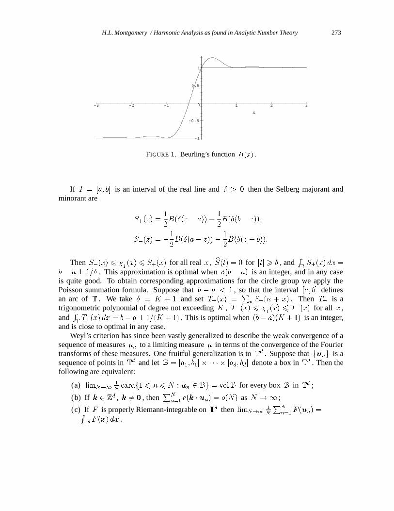
and observed that B(z) = O(e2�j=zj) , that B(x) > sgn(x) for all real x , and thatZR
B(x)� sgn(x) dx = 1 :
Indeed, Beurling showed that among functions with the prior properties, this function unique-ly minimizes the above integral.
H.L. Montgomery / Harmonic Analysis as found in Analytic Number Theory 273
-1
-0.5
0
0.5
1
-3 -2 -1 1 2 3
x
FIGURE 1. Beurling’s function B(x) .
If I = [a; b] is an interval of the real line and Æ > 0 then the Selberg majorant andminorant are
S+(z) =1
2B(Æ(z � a)) +
1
2B(Æ(b� z));
S�(z) = �1
2B(Æ(a� z))� 1
2B(Æ(z � b)):
Then S�(x) 6 �I(x) 6 S+(x) for all real x , bS(t) = 0 for jtj > Æ , and
RRS�(x) dx =
b � a � 1=Æ . This approximation is optimal when Æ(b � a) is an integer, and in any caseis quite good. To obtain corresponding approximations for the circle group we apply thePoisson summation formula. Suppose that b � a < 1 , so that the interval [a; b] definesan arc of T . We take Æ = K + 1 and set T�(x) =
PnS�(n + x) . Then T� is a
trigonometric polynomial of degree not exceeding K , T�(x) 6 �I(x) 6 T+(x) for all x ,
andRTT�(x) dx = b� a� 1=(K + 1) . This is optimal when (b� a)(K + 1) is an integer,
and is close to optimal in any case.Weyl’s criterion has since been vastly generalized to describe the weak convergence of a
sequence of measures �n to a limiting measure � in terms of the convergence of the Fouriertransforms of these measures. One fruitful generalization is to Td . Suppose that fung is asequence of points in Td and let B = [a1; b1]� � � � � [ad; bd] denote a box in Td . Then thefollowing are equivalent:
(a) limN!11
Ncardf1 6 n 6 N : un 2 Bg = volB for every box B in Td ;
(b) If k 2 Zd , k 6= 0 , thenP
N
n=1e(k � un) = o(N) as N !1 ;
(c) If F is properly Riemann-integrable on Td then limN!11
N
PN
n=1F (un) =R
Td F (x) dx .
274 H.L. Montgomery / Harmonic Analysis as found in Analytic Number Theory
Quantitative majorants in Td are easily obtained by forming a product of one-dimen-sional majorants. Minorants are a little more elusive, but Barton, Vaaler and Montgomery [2]have given a construction that works pretty well.
In the same way that we used Weyl’s Criterion to see that the sequence fn�g is uniformlydistributed if � is irrational, we can use Weyl’s Criterion for Td to obtain a sharpening ofKronecker’s Theorem. Suppose that 1; �1; : : : ; �d are linearly independent over the field Q
of rational numbers. Then the points n� = (n�1; n�2; : : : ; n�d) are not only dense in Td
(Kronecker’s Theorem) but are actually uniformly distributed. Indeed, suppose that B is abox in Td , and let T (x) be a trigonometric polynomial that minorizes �
Bwith
RTd T > 0 .
Then
cardfM + 1 6 n 6M +N : n� 2 Bg >M+NXn=M+1
T (n�)
=Xk
bT (k) M+NXn=M+1
e(nk � �)
> N bT (0)� 1
2
Xk 6=0
jbT (k)jkk � �k :
Here the last sum is finite because there are only finitely many k for which bT (k) 6= 0 andbecause k � � is never an integer. Since bT (0) > 0 , the above is positive if N is sufficientlylarge. The remarkable feature here is that the expression above is independent of M . That is,if n1 < n2 < n3 < � � � are the n for which n� 2 B then the gaps ni+1� ni are uniformlybounded above. This insight is critical to Bohr’s definition of almost periodicity.
DEFINITION 2. Let f : R ! C be continuous. We say that a real number t is an "
-almost period of f if jf(x + t) � f(x)j < " for all real x . The function f is almostperiodic if for every " > 0 there is a number C = C(") such that any interval of length atleast C contains an " -almost period.
It is by the strengthened form of Kronecker’s Theorem that we see that the almost periodicpolynomial
T (x) =
NXn=1
ane(�nx)
is indeed an almost periodic function. It can also be shown that the almost periodic poly-nomials are dense in the space of almost periodic functions. Let �(s) =
P1
n=1n�s be the
Riemann zeta function. We write s = �+it . If � is fixed, � > 1 , then �(�+it) is an almostperiodic function of t . The concept of almost periodicity can be generalized to other norms.For example, when � is fixed, 1=2 < � < 1 the function �(�+ it) is a mean-square almostperiodic function, even though it is not an almost periodic function in the uniform norm. One
H.L. Montgomery / Harmonic Analysis as found in Analytic Number Theory 275
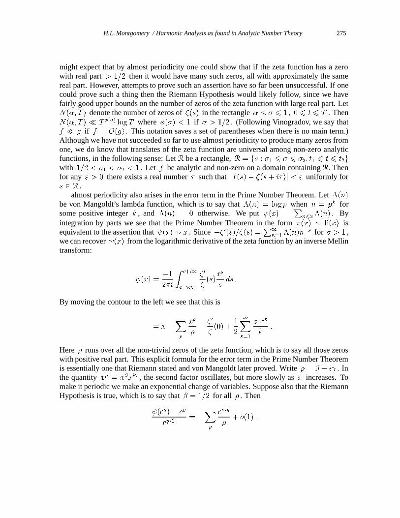
might expect that by almost periodicity one could show that if the zeta function has a zerowith real part > 1=2 then it would have many such zeros, all with approximately the samereal part. However, attempts to prove such an assertion have so far been unsuccessful. If onecould prove such a thing then the Riemann Hypothesis would likely follow, since we havefairly good upper bounds on the number of zeros of the zeta function with large real part. LetN(�; T ) denote the number of zeros of �(s) in the rectangle � 6 � 6 1 , 0 6 t 6 T . ThenN(�; T ) � T
�(�) logT where �(�) < 1 if � > 1=2 . (Following Vinogradov, we say thatf � g if f = O(g) . This notation saves a set of parentheses when there is no main term.)Although we have not succeeded so far to use almost periodicity to produce many zeros fromone, we do know that translates of the zeta function are universal among non-zero analyticfunctions, in the following sense: Let R be a rectangle, R = fs : �1 6 � 6 �2; t1 6 t 6 t2gwith 1=2 < �1 < �2 < 1 . Let f be analytic and non-zero on a domain containing R. Thenfor any " > 0 there exists a real number � such that jf(s)� �(s + i�)j < " uniformly fors 2 R .
almost periodicity also arises in the error term in the Prime Number Theorem. Let �(n)
be von Mangoldt’s lambda function, which is to say that �(n) = log p when n = pk for
some positive integer k , and �(n) = 0 otherwise. We put (x) =P
n6x�(n) . Byintegration by parts we see that the Prime Number Theorem in the form �(x) � li(x) isequivalent to the assertion that (x) � x . Since �� 0(s)=�(s) =P1
n=1�(n)n�s for � > 1 ,
we can recover (x) from the logarithmic derivative of the zeta function by an inverse Mellintransform:
(x) =�12�i
Zc+i1
c�i1
�0
�(s)
xs
sds :
By moving the contour to the left we see that this is
= x�X�
x�
�� �
0
�(0) +
1
2
1Xk=1
x�2k
k:
Here � runs over all the non-trivial zeros of the zeta function, which is to say all those zeroswith positive real part. This explicit formula for the error term in the Prime Number Theoremis essentially one that Riemann stated and von Mangoldt later proved. Write � = � + i . Inthe quantity x
� = x�xi , the second factor oscillates, but more slowly as x increases. To
make it periodic we make an exponential change of variables. Suppose also that the RiemannHypothesis is true, which is to say that � = 1=2 for all � . Then
(ey)� ey
ey=2= �
X�
ei y
�+ o(1) :
276 H.L. Montgomery / Harmonic Analysis as found in Analytic Number Theory
This expression is mean-square almost periodic, and the sum on the right is its Fourier ex-pansion. It is generally believed that the > 0 are linearly independent over Q , so that theterms ei y behave like independent random variables.
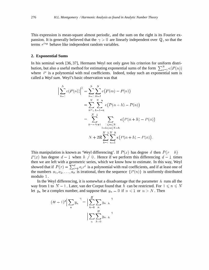
2. Exponential Sums
In his seminal work [36, 37], Hermann Weyl not only gave his criterion for uniform distri-bution, but also a useful method for estimating exponential sums of the form
PN
n=1e(P (n))
where P is a polynomial with real coefficients. Indeed, today such an exponential sum iscalled a Weyl sum. Weyl’s basic observation was that
��� NXn=1
e(P (n))
���2 = NXn=1
NXm=1
e�P (m)� P (n)
�
=
NXn=1
N�nXh=1�n
e�P (n+ h)� P (n)
�
=
N�1Xh=�N+1
X16n6N
1�h6n6N�h
e�P (n+ h)� P (n)
�
= N + 2<N�1Xh=1
N�hXn=1
e�P (n+ h)� P (n)
�:
This manipulation is known as ‘Weyl differencing’. If P (x) has degree d then P (x+ h)�P (x) has degree d � 1 when h 6= 0 . Hence if we perform this differencing d � 1 timesthen we are left with a geometric series, which we know how to estimate. In this way, Weylshowed that if P (x) =
Pd
i=0aix
i is a polynomial with real coefficients, and if at least one ofthe numbers a1; a2; : : : ; ad is irrational, then the sequence fP (n)g is uniformly distributedmodulo 1 .
In the Weyl differencing, it is somewhat a disadvantage that the parameter h runs all theway from 1 to N � 1 . Later, van der Corput found that h can be restricted. For 1 6 n 6 N
let yn be a complex number, and suppose that yn = 0 if n < 1 or n > N . Then
(H + 1)2���X
n
yn
���2 = ��� HXh=0
Xn
yn+h
���2
=
���Xn
HXh=0
yn+h
���2
H.L. Montgomery / Harmonic Analysis as found in Analytic Number Theory 277
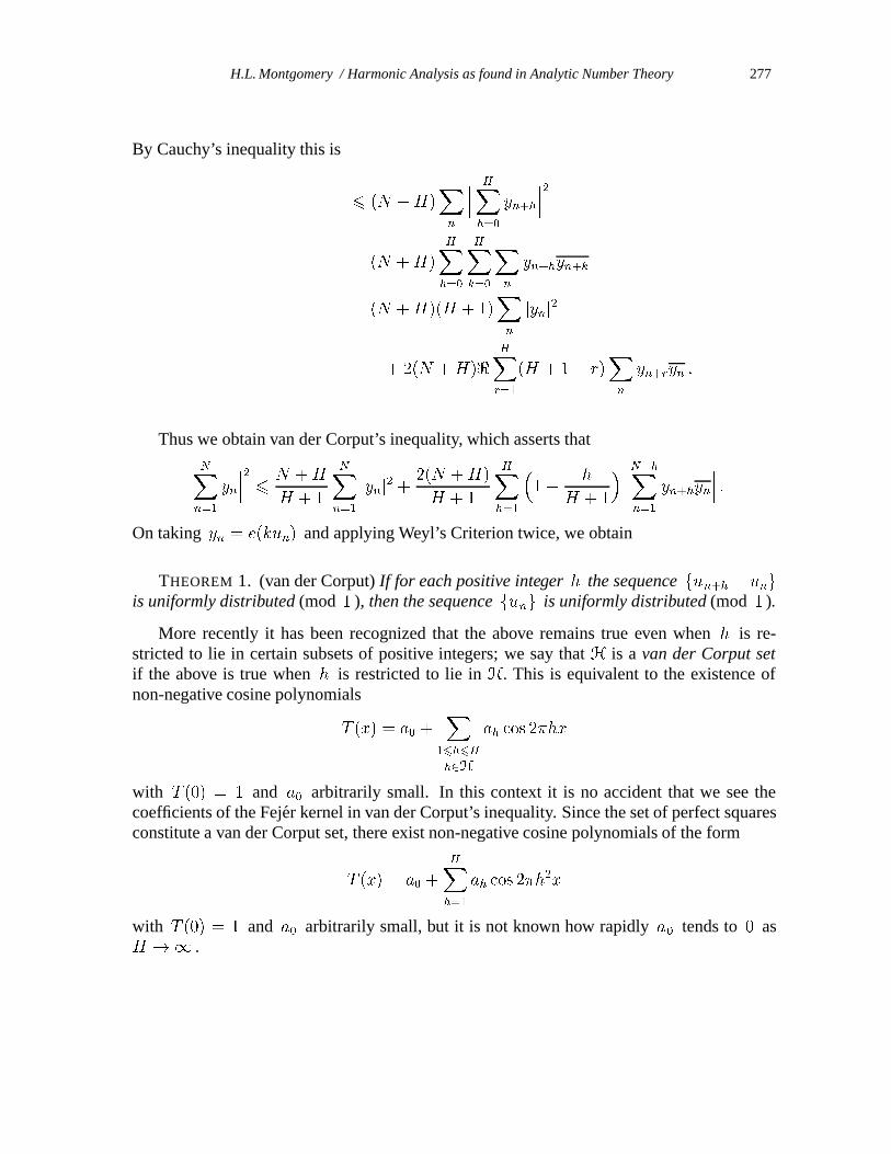
By Cauchy’s inequality this is
6 (N +H)Xn
��� HXh=0
yn+h
���2
= (N +H)
HXh=0
HXk=0
Xn
yn+hyn+k
= (N +H)(H + 1)Xn
jynj2
+ 2(N +H)<HXr=1
(H + 1� r)Xn
yn+ryn :
Thus we obtain van der Corput’s inequality, which asserts that��� NXn=1
yn
���2 6 N +H
H + 1
NXn=1
jynj2 + 2(N +H)
H + 1
HXh=1
�1� h
H + 1
���� N�hXn=1
yn+hyn
��� :On taking yn = e(kun) and applying Weyl’s Criterion twice, we obtain
THEOREM 1. (van der Corput) If for each positive integer h the sequence fun+h � ungis uniformly distributed (mod 1 ), then the sequence fung is uniformly distributed (mod 1 ).
More recently it has been recognized that the above remains true even when h is re-stricted to lie in certain subsets of positive integers; we say that H is a van der Corput setif the above is true when h is restricted to lie in H. This is equivalent to the existence ofnon-negative cosine polynomials
T (x) = a0 +X
16h6H
h2H
ah cos 2�hx
with T (0) = 1 and a0 arbitrarily small. In this context it is no accident that we see thecoefficients of the Fejer kernel in van der Corput’s inequality. Since the set of perfect squaresconstitute a van der Corput set, there exist non-negative cosine polynomials of the form
T (x) = a0 +
HXh=1
ah cos 2�h2x
with T (0) = 1 and a0 arbitrarily small, but it is not known how rapidly a0 tends to 0 asH !1 .
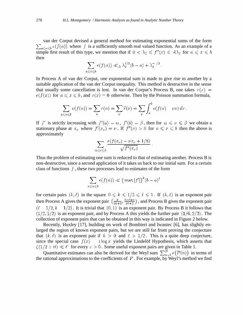
278 H.L. Montgomery / Harmonic Analysis as found in Analytic Number Theory
van der Corput devised a general method for estimating exponential sums of the formPa6n6b
e(f(n)) where f is a sufficiently smooth real valued function. As an example of asimple first result of this type, we mention that if 0 < �2 6 f
00(x) 6 A�2 for a 6 x 6 b
then Xa6n6b
e(f(n))�A �1=2
2(b� a) + �
�1=2
2:
In Process A of van der Corput, one exponential sum is made to give rise to another by asuitable application of the van der Corput inequality. This method is destructive in the sensethat usually some cancellation is lost. In van der Corput’s Process B, one takes r(x) =
e(f(x)) for a 6 x 6 b , and r(x) = 0 otherwise. Then by the Poisson summation formula,
Xa6n6b
e(f(n)) =Xn
r(n) =X�
br(�) =X�
Zb
a
e(f(x)� �x) dx :
If f 0 is strictly increasing with f0(a) = � , f 0(b) = � , then for � 6 � 6 � we obtain a
stationary phase at x� where f0(x�) = � . If f 00(x) > 0 for a 6 x 6 b then the above is
approximately X�6�6�
e(f(x�)� �x� + 1=8)pf 00(x�)
:
Thus the problem of estimating one sum is reduced to that of estimating another. Process B isnon-destructive, since a second application of it takes us back to our initial sum. For a certainclass of functions f , these two processes lead to estimates of the formX
a6n6b
e(f(n))� �max jf 0j�k(b� a)`
for certain pairs (k; `) in the square 0 6 k 6 1=2 6 ` 6 1 . If (k; `) is an exponent pairthen Process A gives the exponent pair
�k
2k+2;k+`+1
2k+2
�, and Process B gives the exponent pair
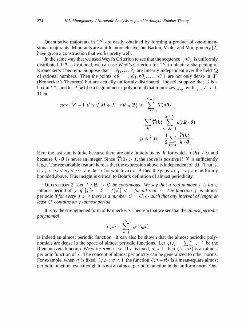
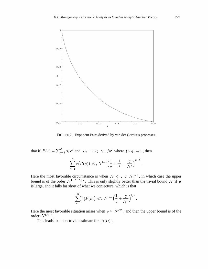
(` � 1=2; k + 1=2) . It is trivial that (0; 1) is an exponent pair. By Process B it follows that(1=2; 1=2) is an exponent pair, and by Process A this yields the further pair (1=6; 2=3) . Thecollection of exponent pairs that can be obtained in this way is indicated in Figure 2 below.
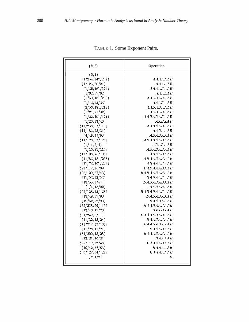
Recently, Huxley [17], building on work of Bombieri and Iwaniec [6], has slightly en-larged the region of known exponent pairs, but we are still far from proving the conjecturethat (k; `) is an exponent pair if k > 0 and ` > 1=2 . This is a quite deep conjecture,since the special case f(x) = t log x yields the Lindelof Hypothesis, which asserts that�(1=2 + it)� t
" for every " > 0 . Some useful exponent pairs are given in Table 1.Quantitative estimates can also be derived for the Weyl sum
PN
n=1e�P (n)
�in terms of
the rational approximations to the coefficients of P . For example, by Weyl’s method we find
H.L. Montgomery / Harmonic Analysis as found in Analytic Number Theory 279
0.5
0.6
0.7
0.8
0.9
1
l
0.1 0.2 0.3 0.4 0.5k
FIGURE 2. Exponent Pairs derived by van der Corput’s processes.
that if P (x) =P
d
i=0�ix
i and j�d � a=qj 6 1=q2 where (a; q) = 1 , then
NXn=1
e�P (n)
��d N1+"
�1q+
1
N+
q
Nd
�21�d
:
Here the most favorable circumstance is when N 6 q 6 Nd�1 , in which case the upper
bound is of the order N 1�21�d
+" . This is only slightly better than the trivial bound N if dis large, and it falls far short of what we conjecture, which is that
NXn=1
e�P (n)
��d N1+"
�1q+
q
Nd
�1=d
:
Here the most favorable situation arises when q � Nd=2 , and then the upper bound is of the
order N1=2+" .This leads to a non-trivial estimate for jS(�)j .
280 H.L. Montgomery / Harmonic Analysis as found in Analytic Number Theory
TABLE 1. Some Exponent Pairs.
(k ;`) Operation
(0;1)
(1=254;247=254) AAAAAAB
(1=126;20=21) AAAAAB
(1=86;161=172) AAAABAAB
(1=62;57=62) AAAAAB
(1=50;181=200) AAABABAAB
(1=42;25=28) AAABAAB
(2=53;181=212) AABABAAAB
(1=24;27=32) AABABAAB
(1=22;101=121) AABABABAAB
(1=20;33=40) AABAAB
(13=238;97=119) AABAABAAB
(11=186;25=31) AABAAAB
(4=49;75=98) ABABAAAB
(11=128;97=128) ABABAABAAB
(1=11;3=4) ABABAAB
(1=10;81=110) ABABABAAB
(13=106;75=106) ABAABAAB
(11=86;181=258) ABAABABAAB
(11=78;161=234) ABAAABAAB
(22=117;25=39) BABAAABAAB
(26=129;27=43) BABAABABAAB
(11=53;33=53) BABAABAAB
(13=55;3=5) BABABABAAB
(1=4;13=22) BABABAAB
(33=128;75=128) BABABAABAAB
(13=49;57=98) BABABAAAB
(19=62;52=93) BAABAAAB
(75=238;66=119) BAABAABAAB
(13=40;11=20) BAABAAB
(81=242;6=11) BAABABABAAB
(11=32;13=24) BAABABAAB
(75=212;57=106) BAABABAAAB
(11=28;11=21) BAAABAAB
(81=200;13=25) BAAABABAAB
(13=31;16=31) BAAAAB
(75=172;22=43) BAAAABAAB
(19=42;32=63) BAAAAAB
(60=127;64=127) BAAAAAAB
(1=2;1=2) B
H.L. Montgomery / Harmonic Analysis as found in Analytic Number Theory 281
3. Power Sums
Although we spend a lot of effort to estimate exponential sums, in the opposite direction it issometimes useful to show that a cancelling sum is not always too cancelling. Turan’s methodof power sums provides tools of exactly this sort. Since error terms in analytic number theoryare often expressed as a sum of oscillatory terms (as we have already seen in the case of theerror term in the Prime Number Theorem), Turan’s method assists us in proving that sucherror terms are sometimes large. To exemplify the method, we describe Turan’s First MainTheorem. Let
s� =
NXn=1
bnz�
n
and suppose that jznj > 1 for all n . Suppose that M is a given non-negative integer. Wewish to show that there is a � , M + 1 6 � 6 M + N , such that js�j is not too smallcompared with js0j . To this end we employ a simple duality argument, which is typical ofTuran’s method. Suppose that numbers a� have been determined so that
(3.1) s0 =
N�1X�=0
a�sM+1+� :
Then
js0j 6� N�1X
�=0
ja�j�
max06�6N�1
jsM+1+�j :
By the definition of s� we see that (3.1) asserts that
NXn=1
bn =
NXn=1
bnzM+1
n
N�1X�=0
a�z�
n:
This identity certainly holds for arbitrary bn provided that
1 = zM+1
n
N�1X�=0
a�z�
n
for 1 6 n 6 N . That is, P (z) =P
N�1
�=0a�z
� should be a polynomial of degree at mostN � 1 that satisfies the N conditions P (zn) = z
�M�1
n. Without loss of generality the zn
are distinct, and hence P (z) is uniquely determined. It can be shown thatP
N�1
�=0ja�j 6P
N�1
k=0
�M+k
k
�2k , and thus we find that
maxM+16�6M+N
js�j > c(M;N)js0j

282 H.L. Montgomery / Harmonic Analysis as found in Analytic Number Theory
where
c(M;N) =
� N�1Xk=0
�M + k
k
�2k��1
:
The constant here is best-possible, but it is disappointingly small, since it is only a little largerthan �
N
2e(M +N)
�N�1
:
Suppose that T (x) is an exponential polynomial of N terms and period 1 , say
T (x) =
NXn=1
bne(�nx)
where the �n are integers. Let I be a closed arc of the circle group T , and let L denote thelength of I . Then by Turan’s First Main Theorem, it is easy to show that
maxx2I
jT (x)j >�L
2e
�N�1
maxx2T
jT (x)j :
Although the constant here depends on the number N of terms in T (x) , it is noteworthythat it is independent of the size of the frequencies �n . This inequality makes it possible togive a simple and motivated proof of the Fabry Gap Theorem.
The small constant c(M;N) can be replaced by a larger constant if one is prepared toallow � to run over a range longer than N . In more restricted situations the lower boundcan be very good indeed. For example, suppose that
(3.2) s� =
NXn=1
e(��n):
ThenKX�=1
�1� �
K + 1
�js�j2 =
NXm=1
NXn=1
KX�=1
�1� �
K + 1
�e(�(�m � �n)):
Since the expression is real, we may take real parts to see that the above is
=
NXm=1
NXn=1
KX�=1
�1� �
K + 1
�cos 2��(�m � �n) =
NXm=1
NXn=1
1
2(�K+1(�m � �n)� 1)
where �K+1(�) denotes the Fejer kernel. Since �K+1(�) > 0 for all � , and �K+1(0) =
K + 1 , it follows that the above is
>1
2(K + 1)N � 1
2N
2:
H.L. Montgomery / Harmonic Analysis as found in Analytic Number Theory 283
Thus if K > (1 + ")N then max16�6K js�j > C(")pN , and in particular
max16�62N
js�j >pN=2 :
By working similarly with higher moments one can obtain still better lower bounds overlonger ranges of � : If s� is given by (3.2) and 1 6 m 6 N=2 then there is a � , 1 6 � 6
(12N=m)m such that js�j > 1
4
pmN . It would be useful to have examples to show that this
is close to best-possible.For a more extensive survey of Turan’s method one may consult Montgomery [21], pp.
85–107. For a detailed account of the subject and important applications, one should see thebook of Turan [33].
4. Irregularities of Distribution
We now consider how well-distributed N points can be. If the points are to fall in [0; 1] thenwe could take un = n=N . These points are extremely well-distributed in the sense that thenumber of them in a subinterval [0; �] is N�+O(1) . However, we find that it is not so easyto distribute points well in T2 . Suppose that our points are un = (u1; u2) , let R(�) be therectangle R(�) = [0; �1]� [0; �2] , and let D(�) be the discrepancy function
D(�) = cardf1 6 n 6 N : un 2 R(�)g �N�1�2 :
Roth [30] used a construction suggestive of wavelets to show thatZT2
D(�)2 d�� logN :
Since it is also possible to construct points that are this well-distributed, this solves the prob-lem as to distribution in mean-square. Ostrowski [27] had observed that D(�) � logN
when un = (n=N; np2) . The problem of showing that in any case kDk1 � logN was
solved by Schmidt [31] by means of a complicated induction. However, a curious differencearises here. Roth’s argument generalizes easily to Tk to show that kDk2 �k (logN)(k�1)=2
for any k > 1 . However, Schmidt’s approach has not been extended to k > 2 . It hasbeen conjectured that kDk1 �k (logN)k�1 . This would be best possible, in view of con-structions of Halton [14]. On the other hand, Pollington has recently mounted a waveletapproach to this problem that has led him to conclude that one should be able to show thatkDk1 �k (logN)k=2 , and that this sup norm need not be larger. Hence one should regardthe question of how large kDk1 need be to be a wide open unsolved problem when k > 2 .Halasz [13] devised a variant of Roth’s method that gives Schmidt’s Theorem concerningkDk1 when k = 2 , and also gives the lower bound kDk1 �
plogN when k = 2 . This
is best possible, since Chen [8] has shown that if 0 < p < 1 and k is given, k > 2 , thenthere exists a configuration of N points in Tk for which kDkp �p;k (logN)(k�1)=2 .
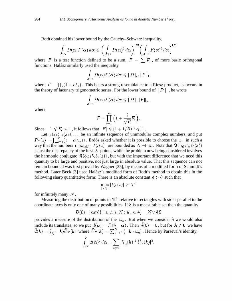
284 H.L. Montgomery / Harmonic Analysis as found in Analytic Number Theory
Roth obtained his lower bound by the Cauchy–Schwarz inequality,ZTk
D(�)F (�) d� 6
�ZTk
D(�)2 d�
�1=2�Z
Tk
F (�)2 d�
�1=2
where F is a test function defined to be a sum, F =PFr , of more basic orthogonal
functions. Halasz similarly used the inequalityZT2
D(�)F (�) d� 6 kDk1kFk1where F =
Qr(1 + cFr) . This bears a strong resemblance to a Riesz product, as occurs in
the theory of lacunary trigonometric series. For the lower bound of kDk1 , he wroteZT2
D(�)F (�) d� 6 kDk1kFk1where
F =
RYr=1
�1 +
ipRFr
�:
Since �1 6 Fr 6 1 , it follows that jF j 6 (1 + 1=R)R � 1 .Let e(x1); e(x2); : : : be an infinite sequence of unimodular complex numbers, and put
PN(z) =Q
N
n=1(z � e(xn)) . Erdos asked whether it is possible to choose the xn in such a
way that the numbers maxjzj61 jPN(z)j are bounded as N !1 . Note that = logPN(e(x))
is just the discrepancy of the first N points, while the problem now being considered involvesthe harmonic conjugate < logPN(e(x)) , but with the important difference that we need thisquantity to be large and positive, not just large in absolute value. That this sequence can notremain bounded was first proved by Wagner [35], by means of a modified form of Schmidt’smethod. Later Beck [3] used Halasz’s modified form of Roth’s method to obtain this in thefollowing sharp quantitative form: There is an absolute constant Æ > 0 such that
maxjzj61
jPN(z)j > NÆ
for infinitely many N .Measuring the distribution of points in Tk relative to rectangles with sides parallel to the
coordinate axes is only one of many possibilities. If S is a measurable set then the quantity
D(S) = cardf1 6 n 6 N : un 2 Sg �N vol S
provides a measure of the distribution of the un . But when we consider S we would alsoinclude its translates, so we put d(�) = D(S+�) . Then bd(0) = 0 , but for k 6= 0 we havebd(k) = b�
S(�k)bUN (k) where bUN(k) =PN
n=1e(�k � un) . Hence by Parseval’s identity,Z
Tk
d(�)2 d� =Xk 6=0
jb�S(k)j2jbUN(k)j2:
H.L. Montgomery / Harmonic Analysis as found in Analytic Number Theory 285
The rate that b�S(k) tends to 0 as k tends to infinity in a particular direction depends on
how much of the boundary of S is orthogonal to the direction in question. Thus in the caseof a rectangle the Fourier coefficients decay slowly in the direction of the coordinate axes,but comparatively rapidly in other directions. Thus one may expect that points may be foundso that bUN (k) is small when b�
S(k) is large, and vice versa. By using the Fejer kernel as in
our discussion of power sums we can show thatXjk1j6X1
jk2j6X2
k 6=0
jbUN (k)j2 > NX1X2 �N2
for any positive real numbers X1; X2 . In this way we can recover Roth’s lower bound forkDk2 . By averaging over disks (and averaging over the radius as well) we find that thereis a disk D for which D(D) � N
1=4 . More generally, if we start with a set S, and areallowed to shrink, translate, and rotate S, then we obtain this larger order of magnitude, inview of a general principle governing the mean square decay of the Fourier transform of thecharacteristic function of a set: If C is a simple, closed, piecewise C
1 curve in R2 , and S isits interior, then Z
jtj>R
jb�S(t)j2 dt � jCj
2�2R
as R!1 . This is due to Montgomery [19], [20] pp. 114–119; see also Herz [15, 16].
5. The Large Sieve
The large sieve was originated by Linnik [18] in a somewhat obscure form. It gained new lifein the hands of Renyi [28], who viewed it as a statement about almost independent vectors.Today we usually think of this as an extension of Bessel’s inequality for vectors in an innerproduct space: Let �1; : : : ; �R be arbitrary vectors in an inner product space. Then thefollowing three assertions concerning the constant C are equivalent:
(a) For any vector � in the space,
RXr=1
j(�; �r)j2 6 Ck�k2;
(b) For any complex numbers ur we have
��� X16r;s6R
urus(�r; �s)
��� 6 C
RXr=1
jcrj2;
(c) C = ��[(�r; �s)]
�.

286 H.L. Montgomery / Harmonic Analysis as found in Analytic Number Theory
(Here �(A) denotes the spectral radius of the matrix A .) Renyi took the coordinates of hisvectors to depend on arithmetic progressions or on Dirichlet characters, but the vectors heobtained in doing so were not very close to orthogonal, so the estimates he obtained wereimperfect. Roth [29] had the excellent idea of taking �r = (e(n�r)) where the �r are well-spaced in T . These vectors are quite close to being orthogonal, and we now think of the mostbasic form of the large sieve as being a statement about the mean square of a trigonometricpolynomial at well-spaced points. That is, we take
S(�) =
M+NXn=M+1
ane(n�);
and we consider inequalities of the shape
RXr=1
jS(�r)j2 6 �
M+NXn=M+1
janj2:
We suppose that k�r � �sk > Æ for r 6= s , and want � to depend on N and Æ . Ifan = e(�n�1) then S(�1) = N , and thus we must have � > N . By averaging overtranslations of the �r we can also show that � > Æ
�1� 1 . We find that � does not have tobe much larger than is required by these considerations.
Gallagher [10] used an inequality of the Sobolev type,
jf(�)j 6 1
Æ
Z�+Æ=2
��Æ=2
jf(x)j dx+1
2
Z�+Æ=2
��Æ=2
jf 0(x)j dx;
to show that one can take � = 1=Æ + �N . This is the best constant with respect to Æ ,but in arithmetic settings the coefficient of N is more important. The main advantage ofGallagher’s approach is that it generalizes readily to other families of functions. To obtaingood dependence on N we note that by duality the stated inequality is equivalent to theinequality
M+NXn=M+1
��� RXr=1
yre(n�r)
���2 6 �
RXr=1
jyrj2:
On the left hand side we square out and take the sum over n inside. The diagonal terms giveNP
rjyrj2 , so it remains to consider the non-diagonal terms. This brings us to Hilbert’s
Inequality, which asserts that ���Xr;s
r 6=s
yrys
r � s
��� 6 �
Xr
jyrj2:
H.L. Montgomery / Harmonic Analysis as found in Analytic Number Theory 287
Montgomery and Vaughan [23], with some assistance from Selberg, found that this can begeneralized, so that ���X
r;s
r 6=s
yrys
�r � �s
��� 6 �
Æ
Xr
jyrj2
provided that j�r � �sj > Æ whenever r 6= s . Moreover for the circle group we have,correspondingly, the inequality���X
r;s
r 6=s
yrys
sin �(�r � �s)
��� 6 1
Æ
Xr
jyrj2
where k�r � �sk > Æ for r 6= s . This gives the large sieve with the factor � = N + 1=Æ .With a little more care one can obtain � = N + 1=Æ � 1 , and with this constant there aresituations in which equality can occur.
In arithmetic situations the �r are usually taken to be the Farey fractions a=q , in which(a; q) = 1 and q 6 Q . Since ka=q � a
0=q0k > 1=(qq0) > 1=Q2 when a=q and a
0=q0 are
distinct modulo 1, we find thatQXq=1
Xa=1
(a;q)=1
jS(a=q)j2 6 (N +Q2)
M+NXn=M+1
janj2:
The generalized Hilbert Inequality can also be established in a weighted form, in whichwe find that ���X
r;s
r 6=s
yrys
�r � �s
��� 6 3
2�
Xr
jyrj2Ær
where j�r � �sj > Ær when s 6= r . Here the constant 3
2� is certainly not best possible. The
above also has a counterpart for the circle group, and hence we have a weighted form of thelarge sieve,
RXr=1
jS(�r)j2N + 3
2Ær
6
M+NXn=M+1
janj2 :
Many other variants of the large sieve have been derived, involving, for example, maxi-mal partial sums (via the Carleson–Hunt Theorem), or the Hardy–Littlewood Maximal Theo-rem. As for further generalizations of Hilbert’s Inequality, Montgomery and Vaaler [22] haveshown that if �r = �r + i r with �r > 0 for all r and j r � sj > Ær for s 6= r , then���X
r;s
r 6=s
yrys
�r + �s
��� 6 84Xr
jyrj2Ær
:
288 H.L. Montgomery / Harmonic Analysis as found in Analytic Number Theory
The proof depends on the theory of H2 functions that are analytic in a half-plane.
6. Dirichlet Series
Let D(s) =P
N
n=1ann
�s . By Hilbert’s Inequality we see thatZT
0
jD(it)j2 dt = (T +O(N))
NXn=1
janj2;
and the weighted Hilbert Inequality givesZT
0
jD(it)j2 dt =NXn=1
janj2(T +O(n)) :
Thus we have some limitation on the amount of time that jDj is large. Suppose that janj 6 1
for all n . Then by applying the above to D2 we find thatZ
T
0
jD(it)j4 dt� (T +N2)N2+"
:
It would be very useful if we could interpolate between these estimates, in the sense thatZT
0
jD(it)jq dt� (T +Nq=2)N q=2+"
for real q , 2 6 q 6 4 . Indeed, this implies the Density Hypothesis concerning the Riemannzeta function. Many years ago, Hardy and Littlewood had conjectured that if j bf(k)j 6 bF (k)
for all k and q > 2 then kfkq �q kFkq , and it can be shown that this majorant conjecturewould imply the conjecture above. However, Bachelis [1] used a method of Katznelson toshow that this is true only when q is an even integer (in which case it holds with constant 1).
In any case there is more that can be said about the number of times a Dirichlet polynomialcan be large than follows from moment estimates. For example, if 0 6 t1 < t2 < : : : < tR 6
T and tr+1 � tr > 1 for all r , if jD(itr)j > V for all r , and if janj 6 1 for all n , thenit is known that R� N
2V�2T" provided that V 2
> NT1=2+" . It has been conjectured that
this estimate for R holds when the last condition is weakened to read V2 > NT
" . However,Bourgain [7] has shown that if this is so then every Kakeya set in Rd , d > 2 , has Hausdorffdimension d . Thus there are those that doubt such a strong conjecture.
7. Spectral Characteristics of Zeros of the Zeta Function
Let h(d) denote the class number of the quadratic number field with discriminant d . In aneffort to derive a useful lower bound for h(d) when d is negative, it was recognized thatit would suffice to have a good supply of pairs of zeros of the Riemann zeta function thatare < c
2�
log tapart where c < 1=2 . With this motivation, an attempt was made in 1971 to
determine the distribution of � 0 as and
0 run over nearby ordinates of zeros of the
H.L. Montgomery / Harmonic Analysis as found in Analytic Number Theory 289
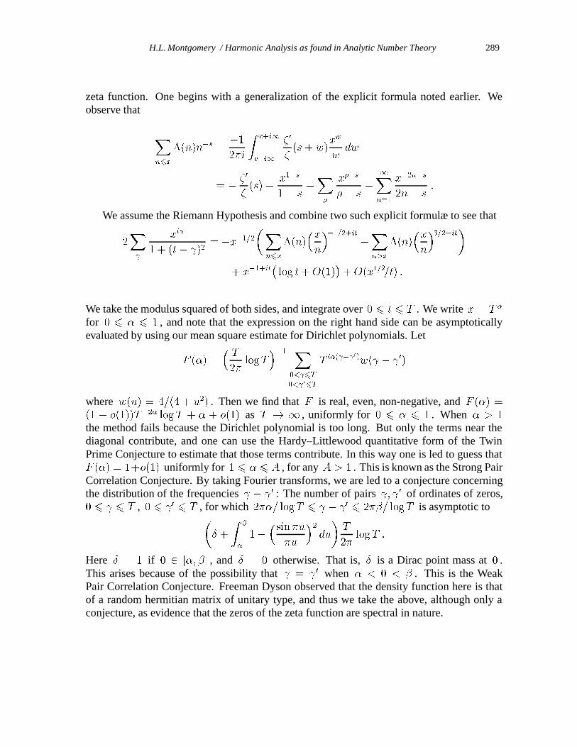
zeta function. One begins with a generalization of the explicit formula noted earlier. Weobserve that
Xn6x
�(n)n�s =�12�i
Zc+i1
c�i1
�0
�(s+ w)
xw
wdw
= � �0
�(s) +
x1�s
1� s�X�
x��s
�� s+
1Xn=1
x�2n�s
2n+ s:
We assume the Riemann Hypothesis and combine two such explicit formulæ to see that
2X
xi
1 + (t� )2= �x�1=2
�Xn6x
�(n)�x
n
��1=2+it
+Xn>x
�(n)�x
n
�3=2+it
�
+ x�1+it
�log t +O(1)
�+O(x1=2=t) :
We take the modulus squared of both sides, and integrate over 0 6 t 6 T . We write x = T�
for 0 6 � 6 1 , and note that the expression on the right hand side can be asymptoticallyevaluated by using our mean square estimate for Dirichlet polynomials. Let
F (�) =�T
2�logT
��1 X0< 6T
0< 06T
Ti�( � 0)
w( � 0)
where w(u) = 4=(4 + u2) . Then we find that F is real, even, non-negative, and F (�) =
(1 + o(1))T�2� logT + � + o(1) as T ! 1 , uniformly for 0 6 � 6 1 . When � > 1
the method fails because the Dirichlet polynomial is too long. But only the terms near thediagonal contribute, and one can use the Hardy–Littlewood quantitative form of the TwinPrime Conjecture to estimate that those terms contribute. In this way one is led to guess thatF (�) = 1+o(1) uniformly for 1 6 � 6 A , for any A > 1 . This is known as the Strong PairCorrelation Conjecture. By taking Fourier transforms, we are led to a conjecture concerningthe distribution of the frequencies �
0 : The number of pairs ; 0 of ordinates of zeros,0 6 6 T , 0 6
0 6 T , for which 2��= logT 6 � 0 6 2��= logT is asymptotic to�
Æ +
Z�
�
1��sin �u
�u
�2
du
�T
2�logT :
Here Æ = 1 if 0 2 [�; �] , and Æ = 0 otherwise. That is, Æ is a Dirac point mass at 0 .This arises because of the possibility that =
0 when � < 0 < � . This is the WeakPair Correlation Conjecture. Freeman Dyson observed that the density function here is thatof a random hermitian matrix of unitary type, and thus we take the above, although only aconjecture, as evidence that the zeros of the zeta function are spectral in nature.
290 H.L. Montgomery / Harmonic Analysis as found in Analytic Number Theory
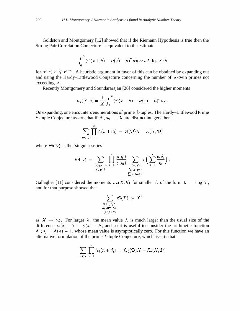
Goldston and Montgomery [12] showed that if the Riemann Hypothesis is true then theStrong Pair Correlation Conjecture is equivalent to the estimate
ZX
0
( (x+ h)� (x)� h)2 dx � hX logX=h
for x" 6 h 6 x1�" . A heuristic argument in favor of this can be obtained by expanding out
and using the Hardy–Littlewood Conjecture concerning the number of d -twin primes notexceeding x .
Recently Montgomery and Soundararajan [26] considered the higher moments
�k(X; h) =1
X
ZX
0
( (x + h)� (x)� h)k dx :
On expanding, one encounters enumerations of prime k-tuples. The Hardy–Littlewood Primek -tuple Conjecture asserts that if d1; d2; : : : dk are distinct integers then
Xn6X
kYi=1
�(n+ di) = S(D)X + E(X;D)
where S(D) is the ‘singular series’
S(D) =X
16qi<1
(16i6k)
kYi=1
�(qi)
�(qi)
X16ai6qi
(ai;qi)=1P
ai=qi2Z
e
� kXi=1
aidi
qi
�:
Gallagher [11] considered the moments �k(X; h) for smaller h of the form h = c logX ,and for that purpose showed that X
06di6X
di distinct
(16i6k)
S(D) � Xk
as X ! 1 . For larger h , the mean value h is much larger than the usual size of thedifference (x + h) � (x) � h , and so it is useful to consider the arithmetic function�0(n) = �(n) � 1 , whose mean value is asymptotically zero. For this function we have analternative formulation of the prime k-tuple Conjecture, which asserts that
Xn6X
kYi=1
�0(n+ di) = S0(D)X + E0(X;D)
H.L. Montgomery / Harmonic Analysis as found in Analytic Number Theory 291
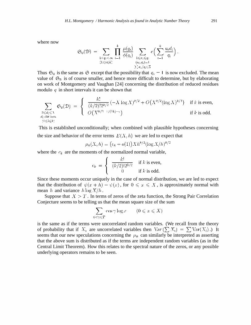
where now
S0(D) =X
1<qi<1
(16i6k)
kYi=1
�(qi)
�(qi)
X16ai6qi
(ai;qi)=1P
ai=qi2Z
e
� kXi=1
aidi
qi
�:
Thus S0 is the same as S except that the possibility that qi = 1 is now excluded. The meanvalue of S0 is of course smaller, and hence more difficult to determine, but by elaboratingon work of Montgomery and Vaughan [24] concerning the distribution of reduced residuesmodulo q in short intervals it can be shown that
X06di6X
di distinct
(16i6k)
S0(D) =
8<:
k!
(k=2)!2k=2(�X logX)k=2 +O
�X
k=2(logX)k=4�
if k is even,
O�X
k=2�1=(7k)+"�
if k is odd.
This is established unconditionally; when combined with plausible hypotheses concerning
the size and behavior of the error terms E(X; h) we are led to expect that
�k(X; h) =�ck + o(1)
�Xh
k=2(logX=h)k=2
where the ck are the moments of the normalized normal variable,
ck =
8<:
k!
(k=2)!2k=2if k is even,
0 if k is odd.
Since these moments occur uniquely in the case of normal distribution, we are led to expectthat the distribution of (x + h) � (x) , for 0 6 x 6 X , is approximately normal withmean h and variance h logX=h .
Suppose that X > T . In terms of zeros of the zeta function, the Strong Pair CorrelationConjecture seems to be telling us that the mean square size of the sumX
0< 6T
cos logx (0 6 x 6 X)
is the same as if the terms were uncorrelated random variables. (We recall from the theoryof probability that if Xi are uncorrelated variables then Var (
PXi) =
PVar(Xi) .) It
seems that our new speculations concerning the �k can similarly be interpreted as assertingthat the above sum is distributed as if the terms are independent random variables (as in theCentral Limit Theorem). How this relates to the spectral nature of the zeros, or any possibleunderlying operators remains to be seen.

292 H.L. Montgomery / Harmonic Analysis as found in Analytic Number Theory
References
[1] G. F. Bachelis, On the upper and lower majorant properties in Lp(G) , Quart. J. Math. (Oxford) (2) 24(1973), 119–128.
[2] J. T. Barton, H. L. Montgomery and J. D. Vaaler, Note on a Diophantine inequality in several variables, toappear.
[3] J. Beck, The modulus of polynomials with zeros on the unit circle: a problem of Erd os, Ann. of Math. (2)134 (1991), 609–651.
[4] J. Beck and W. W. L. Chen, Irregularities of distribution, Cambridge Tract 89, Cambridge University Press,Cambridge, 1987.
[5] A. Beurling, Sur les integrales de Fourier absolument convergentes et leur application a une transforma-tion fonctionelle, Neuvieme congres des mathematiciens scandinaves, Helsingfors, 1938
[6] E. Bombieri and H. Iwaniec, On the order of �( 12+ it) , Ann. Scuola Norm. Sup. Pisa Cl. Sci. (4) 13
(1986), 449–472.[7] J. Bourgain, On the distribution of Dirichlet sums, J. Anal. Math. 60 (1993), 21–32.[8] W. W. L. Chen, On irregularities of distribution, I, Mathematika 27 (1980), 153–170.[9] P. Erdos and P. Turan, On a problem in the theory of uniform distribution I, Nederl. Akad. Wetensch. Proc.
51 (1948), 1146–1154; II, 1262–1269, (= Indag. Math. 10, 370–378; 406–413).[10] P. X. Gallagher, The large sieve, Mathematika 14 (1967), 14–20.[11] , On the distribution of primes in short intervals, Mathematika 23 (1976), 4–9.[12] D. A. Goldston and H. L. Montgomery, On pair correlations of zeros and primes in short intervals, An-
alytic number theory and Diophantine problems (Stillwater, 1984), Birkhauser Verlag, Boston–Basel–Berlin, 1987, 183–203.
[13] G. Halasz, On Roth’s method in the theory of irregularities of point distributions, Recent Progress inAnalytic Number Theory (Durham, 1979), Vol. 2, Academic Press, London, 1981, 79–84.
[14] J. H. Halton, On the efficiency of certain quasirandom sequences of points in evaluating multidimensionalintegrals, Num. Math. 2 (1960), 84–90.
[15] C. S. Herz, Fourier transforms related to convex sets, Ann. of Math. (2) 75 (1961), 81–92.[16] C. S. Herz, On the number of lattice points in a convex set, Amer. J. Math. 84 (1962), 126–133.[17] M. N. Huxley, Area, Lattice Points and Exponential Sums, Clarendon Press, Oxford, 1996.[18] Ju. V. Linnik, The large sieve, Dokl. Akad. Nauk SSSR 30 (1941), 292–294.[19] H. L. Montgomery, The analytic principle of the large sieve, Bull. Amer. Math. Soc. 84 (1978), 547–567.[20] H. L. Montgomery, Irregularities of distribution, Congress of Number Theory (Zarautz, 1984), Universi-
dad del Pais Vasco, Bilbao, 1989, 11–27.[21] H. L. Montgomery, Ten lectures on the interface between analytic number theory and harmonic analysis,
CBMS No. 84, Amer. Math. Soc., Providence, 1994.[22] H. L. Montgomery and J. D. Vaaler, A further generalization of Hilbert’s inequality, Mathematika 45
(1999), 35–39.[23] H. L. Montgomery and R. C. Vaughan, Hilbert’s inequality, J. London Math. Soc. (2) 8 (1974), 73–82.[24] , On the distribution of reduced residues, Annals of Math. 123 (1986), 311–333.[25] H. L. Montgomery and K. Soundararajan, Beyond pair correlation, to appear.[26] H. L. Montgomery and K. Soundararajan, Primes in short intervals, to appear.[27] A. Ostrowski, Bemerkungen zur Theorie der Diophantischen Approximationen I, Abh. Math. Sem. Ham-
burg 1 (1922), 77–98; II, 1 (1922), 250–251; III, 41 (1926), 224.[28] A. Renyi, Un nouveau theoreme concernant les fonctions independantes et ses applications a la theorie
des nombres, J. Math. Pures Appl. 28 (1949), 137–149.[29] K. F. Roth, On irregularities of distribution, Mathematika 1 (1954), 73–79.
H.L. Montgomery / Harmonic Analysis as found in Analytic Number Theory 293
[30] K. F. Roth, On the large sieves of Linnik and Renyi, Mathematika 12 (1965), 1–9.[31] W. M. Schmidt, Irregularities of distribution, VII, Acta Arith. 21 (1972), 49–50.[32] A. Selberg, Collected Papers, Volume II, Springer-Verlag, Berlin, 1991.[33] P. Turan, On a new method of analysis and its applications, Wiley-Interscience, New York, 1984.[34] J. D. Vaaler, Some extremal functions in Fourier analysis, Bull. Amer. Math. Soc. 12 (1985), 183–216.[35] G. S. Wagner, On a problem of Erdos in Diophantine approximation, Bull. London Math. Soc. 12 (1980),
81–88.[36] H. Weyl, Uber ein Problem aus dem Gebiete der diophantischen Approximationen, Nachr. Ges. Wiss.
Gottingen, Math.-phys. Kl. (1914), 234–244; Gesammelte Abhandlungen, Band I, Springer-Verlag,Berlin–Heidelberg–New York, 1968,487–497.
[37] Uber die Gleichverteilung von Zahlen mod. Eins, Math. Ann. 77 (1916), 313–352; Gesammelte Abhand-lungen, Band I, Springer-Verlag, Berlin–Heidelberg–New York, 1968, 563–599; Selecta Hermann Weyl,Birkhauser Verlag, Basel–Stuttgart, 1956, 111–147.