Handbook of Research on Developments and Trends …i.cs.hku.hk/~fcmlau/papers/Chap9.pdfHandbook of...

Handbook of Research on Developments and Trends in Wireless Sensor Networks: From Principle to Practice

Hai JinHuazhong University of Science and Technology, China

Wenbin JiangHuazhong University of Science and Technology, China

Hershey • New YorkInformatIon scIence reference

Director of Editorial Content: Kristin KlingerDirector of Book Publications: Julia MosemannAcquisitions Editor: Mike KillianDevelopment Editor: Beth ArdnerPublishing Assistant: Kurt SmithTypesetter: Devvin EarnestQuality control: Jamie SnavelyCover Design: Lisa TosheffPrinted at: Yurchak Printing Inc.

Published in the United States of America by Information Science Reference (an imprint of IGI Global)701 E. Chocolate AvenueHershey PA 17033Tel: 717-533-8845Fax: 717-533-8661E-mail: [email protected] site: http://www.igi-global.com/reference

Copyright © 2010 by IGI Global. All rights reserved. No part of this publication may be reproduced, stored or distributed in any form or by any means, electronic or mechanical, including photocopying, without written permission from the publisher.

Product or company names used in this set are for identification purposes only. Inclusion of the names of the products or companies does not indicate a claim of ownership by IGI Global of the trademark or registered trademark.

Library of Congress Cataloging-in-Publication Data

Handbook of research on developments and trends in wireless sensor networks : from principle to practice / Hai Jin and Wenbin Jiang, editors. p. cm. Includes bibliographical references and index. Summary: "This book showcases the work many devoted wireless sensor network researchers all over world, and exhibits the up-to-date developments of WSNs from various perspectives"--Provided by publisher. ISBN 978-1-61520-701-5 (hardcover) -- ISBN 978-1-61520-702-2 (ebook) 1. Wireless sensor networks--Research. I. Jin, Hai. II. Jiang, Wenbin. TK7872.D48H357 2010 681'.2--dc22 2009052441

British Cataloguing in Publication DataA Cataloguing in Publication record for this book is available from the British Library.

All work contributed to this book is new, previously-unpublished material. The views expressed in this book are those of the authors, but not necessarily of the publisher.

184

Copyright © 2010, IGI Global. Copying or distributing in print or electronic forms without written permission of IGI Global is prohibited.

Chapter 9

Joint Link Scheduling and Topology Control for

Wireless Sensor Networks with SINR Constraints

Qiang-Sheng HuaThe University of Hong Kong, China

Francis C.M. LauThe University of Hong Kong, China

INTRODUCTION

Cross-layer design of wireless ad-hoc and sensor networks has received increasing attention in the past several years (Goldsmith & Wicker, 2002). Most of these work focused on the interplay among the physical, MAC and network layer, resulting in various joint designs of power control, modulation and coding, link scheduling and routing. Very few

of them, however, have considered joint design with topology control. Topology control (Gao et al., 2008; Santi, 2005) is the strategy to tune the sen-sors’ transmitting powers so that the sensor nodes collectively can maintain a certain global topology such as connectivity. The goal in topology control is to minimize the sensors’ power consumption while trying to provide sufficient network capacity. Topol-ogy control plays a very important role in wireless sensor networks: first, the packets are sent via radio

ABSTRACT

This chapter studies the joint link scheduling and topology control problems in wireless sensor networks. Given arbitrarily located sensor nodes on a plane, the task is to schedule all the wireless links (each representing a wireless transmission) between adjacent sensors using a minimum number of timeslots. There are two requirements for these problems: first, all the links must satisfy a certain property, such as that the wireless links form a data gathering tree towards the sink node; second, all the links simul-taneously scheduled in the same timeslot must satisfy the SINR constraints. This chapter focuses on various scheduling algorithms for both arbitrarily constructed link topologies and the data gathering tree topology. We also discuss possible research directions.

DOI: 10.4018/978-1-61520-701-5.ch009

185

Joint Link Scheduling and Topology Control for Wireless Sensor Networks with SINR Constraints

transmissions by which there must be a connected topology (or other topologies, such as t-spanner) to guarantee that the information collected at each sensor can be forwarded to the other sen-sors; second, since all the sensor nodes are power limited, energy efficiency is a fundamental chal-lenge in sensor networks; third, a high throughput capacity can ensure the collected information to be more quickly sent to the sink nodes, which is crucial in many critical sensor applications. The higher throughput capacity achieved by topol-ogy control in wireless sensor networks can be realized by reducing the network’s interferences (Wattenhofer et al., 2001), the degree of which is generally considered to be directly related to the sensor network’s maximum node degree (Wang & Li, 2003). Such interference degree, as well as the other graph-based interference models devel-oped later by many other researchers (Schmid & Wattenhofer, 2006), however, can not accurately reflect the actual capacity gains of wireless sensor networks in reality. For example, it has been shown that low node degree does not necessarily mean low interference degree (Burkhart et al., 2004), and a higher graph-based interference degree does not necessarily mean lower network capac-ity (Hua & Lau, 2008). In this chapter, we study two related joint link scheduling and topology control problems, the goal of which is to minimize the number of timeslots used to schedule all the wireless links (transmissions) in any given topol-ogy or a specifically constructed topology. Here the number of timeslots used corresponds to the reciprocal of the network capacity.

SYSTEM MODEL AND PROBLEM DEFINITIONS

System Model

We have the following assumptions: (1) All the stationary wireless sensors are arbitrarily located on a plane, and each sensor is equipped

with an omni-directional antenna; (2) we assume a single channel and half-duplex mode, which means each sensor can not send to or receive from more than one node, nor to receive and send at the same time; (3) the link capacity is fixed, which means increasing the transmission power only increases its transmitting range but not its capacity; (4) time is slotted with equal durations; (5) we assume the signal-to-interference-plus-noise ratio (SINR) model is applied, which is a popular model approximating the physical reality of signal transmission in a wireless net-work. The SINR model is more realistic than the graph-based interference models, which also makes our link scheduling problems much more challenging.

The SINR ratio at the receiver of a link i can be represented as (Gupta & Kumar, 2000):

SINRg p

n g pi

ii i

i ij jj j i

Q=

×

+ ×³

= ¹å 1,

b

(The SINR model)

where pidenotes the transmission power of link

i’s transmitter is

; ni is the background noise at

link i’s receiver ir

; gii

andgij are the link gain

from is

to ir

, and that from link j’s transmitterjs to i

r, respectively; Q denotes the number of

simultaneous transmissions with link i; b is the SINR threshold which is larger than or equal to 1. Here the numeratorg p

ii i× means the received

power at ir

. In the denominator,g pij j× means the

attenuated power of pjat i

rand it is regarded as the

interference power for link i, thus g pij jj j i

Q×

= ¹å 1,

means the accumulated interferences caused by all the other simultaneous transmissions. Since we do not consider fading effects and possible obstacles in wireless transmissions, the link gain can be represented by an inverse power law model of the link length, i.e., g d i i

ii s r= 1/ ( , )a

andg d j iij s r= 1/ ( , )a . Here d(, ) is the Euclidean

distance function, anda is the path loss exponent

186


which is equal to 2 in free space, and varies be-tween 2 and 6 in urban areas.

We define a non-negativeQ Q´ link gain matrixH h

ij= ( ) such thath g g

ij ij ii= ×b / , for

i j¹ , andhij= 0 , for i j= . We also define a

noise vector h h= ( )i

such that h bi i ii

n g= × / . With these definitions, we can rewrite the SINR inequality as p h p

i ij j ij

Q= × +

=å h1

. By using a vector-matrix notation, the above inequality be-comesP HP³ + h , or( )I H P- ³ h . If there is only one transmitting link, i.e., no interferences from other links, the SINR model degenerates into the SNR (Signal to Noise Ratio) model, which is shown below:

p n d i ii i s r³ × ×b a( , ) (The SNR model)

Obviously, the SNR model defines the mini-mum power of link i’s transmitteri

sto use such that

the receiver ir

can successfully decode the packet. We now define the spectral radius r( )H of the H matrix asr l( ) max | ( ) |H H

i i= wherel

iH( )stands

for the ith eigenvalue of H. Let riandc

j represent

the ith row sum and jth column sum of H, and we have: r h

i ijj= å andc h

j iji= å . Now according

to (Andersin et al., 1996), we know the matrix H is a non-negative irreducible matrix. Also by compiling the propositions proposed in (Pillai et al., 2005, Zander, 1992b), we have the following useful properties of the H matrix:

Property 1:r( )H increases when any entry of H increases.

Since h d i i d j iij s r s r= ×b a a( , ) / ( , ) , we can

see that r( )H can be reduced by either reducing the threshold valueb , the length of any links or by selecting the links which can result in larger d j i

s r( , )values.

Property 2: min( ) ( ) max( )i i i i

r H r£ £r ;min( ) ( ) max( )

j j j jc H c£ £r .

Property 3: ( )I H- >-1 0 if and only ifr( )H < 1 .

P ro p e r t y 4 : T h e p o w e r v e c t o rP I H* ( )= - ×-1 h is Pareto-optimal in the sense

that P P* ³ component-wise for any other non-negativeP satisfying( )I H P- ³ h .

Problem Definitions

In this chapter, we study two closely related joint link scheduling and topology control problems. The first (MLSAT) is for given arbitrary link to-pologies, and the second (MLSTT) is for forming a data gathering tree topology. Note that, from the following problem definitions, we can easily see that if the tree topology has been constructed, MLSTT becomes a special case of MLSAT. The MLSAT problem is a prominent open problem (Locher, Rickenbach & Wattenhofer, 2008). However, as we will see, how to construct the tree topology plays a very important role in the scheduling length. In addition, for the two prob-lems, we assume each link has one packet to be transmitted. In this case, we can take the totally used timeslots T (the scheduling length) as the frame length, which means that the scheduling sequence will be repeated in the subsequent frames, i.e., X X

i t i t k T, ,= + × ( 0 < £t T ; k is a

positive integer;Xi t,

equals 1 if link i transmits in timeslot t and 0 otherwise).

Problem MLSAT (Minimum Frame Length Link Scheduling for Arbitrary Topologies):

Given n links which are arbitrarily constructed over arbitrarily located sensors on a plane, assign each link’s transmitting sensor a power level and a timeslot, such that all the links scheduled in the same timeslot satisfy the SINR constraints and the number of timeslots used is minimized.

Problem MLSTT (Minimum Frame Length Link Scheduling for a Data Gathering Tree To-pology):

Given n sensors arbitrarily located on a plane, connect these sensors to form a data gathering tree towards the sink such that the number of timeslots used to schedule all the constructed links under the SINR model is minimized.

187


Examples

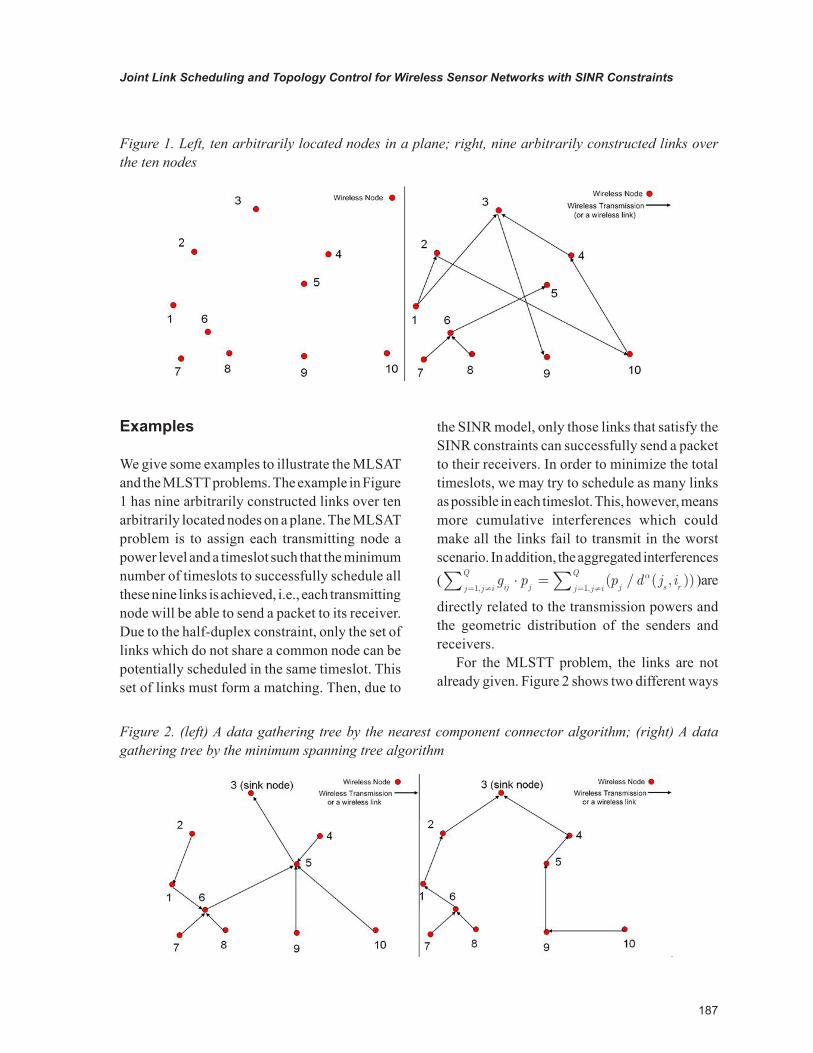
We give some examples to illustrate the MLSAT and the MLSTT problems. The example in Figure 1 has nine arbitrarily constructed links over ten arbitrarily located nodes on a plane. The MLSAT problem is to assign each transmitting node a power level and a timeslot such that the minimum number of timeslots to successfully schedule all these nine links is achieved, i.e., each transmitting node will be able to send a packet to its receiver. Due to the half-duplex constraint, only the set of links which do not share a common node can be potentially scheduled in the same timeslot. This set of links must form a matching. Then, due to

the SINR model, only those links that satisfy the SINR constraints can successfully send a packet to their receivers. In order to minimize the total timeslots, we may try to schedule as many links as possible in each timeslot. This, however, means more cumulative interferences which could make all the links fail to transmit in the worst scenario. In addition, the aggregated interferences ( g p p d j i

ij jj j i

Q

j j i

Q

j s r× =

= ¹ = ¹å å1 1, ,( / ( , ))a ) are

directly related to the transmission powers and the geometric distribution of the senders and receivers.

For the MLSTT problem, the links are not already given. Figure 2 shows two different ways

Figure 1. Left, ten arbitrarily located nodes in a plane; right, nine arbitrarily constructed links over the ten nodes

Figure 2. (left) A data gathering tree by the nearest component connector algorithm; (right) A data gathering tree by the minimum spanning tree algorithm

188


to connect the sensors as a tree towards the sink node. The left side is a tree constructed via the nearest component connector algorithm presented in (Fussen, 2004), and the right side is constructed by a minimum spanning tree algorithm. By our discussion about interferences in the last para-graph, different ways of connecting the nodes may result in different scheduling lengths. In tackling the MLSTT problem, the scheduling strategy must be jointly considered with the topology construction algorithm.

We will give further examples in the following to elucidate our link scheduling problems under the SINR model.

THE FOUR FACTORS THAT IMPACT THE SCHEDULING LENGTH

In this section, we discuss the four factors that have a significant influence on the scheduling length of our scheduling problems.

Power Assignment Strategies Make a Difference

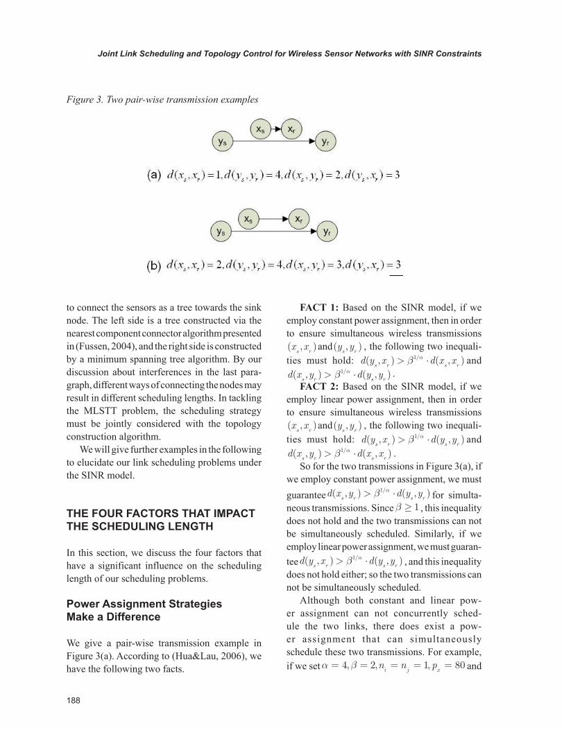
We give a pair-wise transmission example in Figure 3(a). According to (Hua&Lau, 2006), we have the following two facts.

FACT 1: Based on the SINR model, if we employ constant power assignment, then in order to ensure simultaneous wireless transmissions ( , )x x

s rand( , )y y

s r, the following two inequali-

ties must hold: d y x d x xs r s r

( , ) ( , )/> ×b a1 andd x y d y y

s r s r( , ) ( , )/> ×b a1 .

FACT 2: Based on the SINR model, if we employ linear power assignment, then in order to ensure simultaneous wireless transmissions ( , )x x

s rand( , )y y

s r, the following two inequali-

ties must hold: d y x d y ys r s r

( , ) ( , )/> ×b a1 andd x y d x x

s r s r( , ) ( , )/> ×b a1 .

So for the two transmissions in Figure 3(a), if we employ constant power assignment, we must guaranteed x y d y y

s r s r( , ) ( , )/> ×b a1 for simulta-

neous transmissions. Sinceb ³ 1 , this inequality does not hold and the two transmissions can not be simultaneously scheduled. Similarly, if we employ linear power assignment, we must guaran-teed y x d y y

s r s r( , ) ( , )/> ×b a1 , and this inequality

does not hold either; so the two transmissions can not be simultaneously scheduled.

Although both constant and linear pow-er assignment can not concurrently sched-ule the two links, there does exist a pow-er assignment that can simultaneously schedule these two transmissions. For example, if we seta b= = = = =4 2 1 80, , ,n n p

i j x and

Figure 3. Two pair-wise transmission examples

189


py= 3150 , we can compute the SINR values for

transmissions ( , )x xs r and( , )y y

s r . Since

SINRx= + >( / ) / ( / ) .80 1 1 3150 3 2 001 24 4

and SINR

y= + >( / ) / ( / ) .3150 4 1 80 2 2 051 24 4

we can see that these two links can be scheduled in the same timeslot.

From this example, we can conclude that, in order to minimize the total scheduling length, picking the right power assignment strategy is of paramount importance.

Link Topologies Make a Difference

Link topology refers to the geometric distributions of all the senders and receivers of the wireless links. We take the two of the links in Figure 3(b) as an example. Also according to (Hua&Lau, 2006), we have the following fact.

FA C T 3 : B a s e d o n t h e S I N R model, for any pair-wise wireless trans-missions ( , )x x

s r and ( , )y ys r , if we have

d x y d y x d x x d y ys r s r s r s r

( , ) ( , ) ( , ) ( , )/× £ × ×b a2 , then there does not exist any power assignment strategy that can simultaneously schedule the two links.

For example, for the two links in Figure 3(b), if we set a = 4 andb = 2 , then since

2/

2/4

( , ) ( , ) 3 39 ( , ) ( , )2 2 4 11.31

s r s r

s r s r

d x y d y xd x x d y yαβ

⋅ = ⋅

= < ⋅ ⋅

= ⋅ ⋅ �

we can see that there are no power assignment strategies that can schedule the two links in the same timeslot.

From this example, we can see that, in a joint link scheduling and topology control algorithm, we must construct a topology that can avoid as many as possible of these pair-wise wireless links that cannot be simultaneously transmitted. In other words, we must find a topology that can take full

advantage of power control to schedule as many links as possible in every timeslot.

Length Diversities Make a Difference

The link topology shown in Figure 4 has a length diversity of 1. This link topology is called a parallel link array and is borrowed from (Baccelli et al. 2006). We now give a theorem which states that this link topology can be scheduled in a constant number of timeslots.

THEOREM 1: The parallel link array given in Figure 4 can be scheduled in m timeslots where m is a constant that satisfiesm ³ -( / ( )) /2 1 1ab a a .

PROOF: In each timeslot, as shown in Fig-ure 4, we just pick all the links where each pair of nearby links has equal horizontal separation distanced mh= . If we can prove that all of these links can be successfully scheduled in one timeslot, we can then deduce that the total links can be scheduled in m timeslots. So we need to prove that all the links we pick in each timeslot do satisfy the SINR constraints.

Suppose we use constant power assignment, i.e., all the simultaneously scheduled links employ the same transmission power P. The SINR value for every link i scheduled in the same timeslots is:

2 2 /2

/(2 / (( 1) ))

/(2 / ( ))

/ 2 (1 / )

ii

k

ik

ik

P hSINRn P k m h

P hn P k m h

mn m h P k

α

α α

α

α α α

α

α α α

=+ ⋅ +∑

≥+ ⋅∑

=⋅ ⋅ + ⋅∑

Suppose t he t r ansmis s ion powerP n m h

i × ×a a . Then due to a standard Ri-

emann Zeta Function, the above SINR inequality becomes

SINRm

k

mi

k

a

a

a aa2 1

1

2×³

× -×å( / )

( )

190


So as long asm ³ -( / ( )) /2 1 1ab a a , we haveSINR

i³ b . This completes the proof.

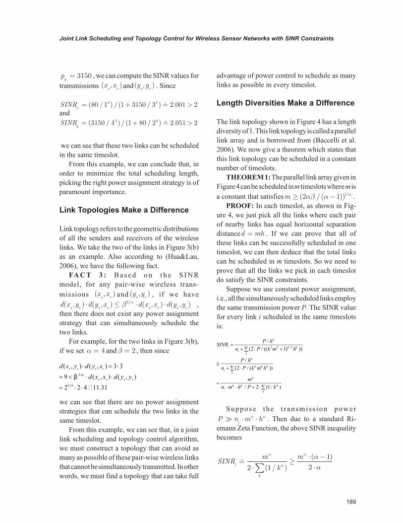
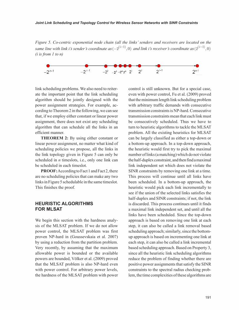
Another link topology is given in Figure 5, whose length diversity equals n which is the number of the links. We call this link topology co-centric exponential node chain and it was first used in (Moscibroda et al. 2007). We set the path loss exponenta = 3 , the background noisen

i= 0 and the thresholdb = 2 . The best heu-

ristic link scheduling algorithm so far employs a novel nonlinear power assignment strategy for this link topology, which is presented in (Moscibroda et al. 2007); it can schedule all of these n links inO n(log ) timeslot. Here we need to point out that, considering arbitrary power assignment strategy, no better upper bound or any lower bound of this link topology’s scheduling length is known.

From the above, we can see that, for a set of links, the length diversity of the link topology plays a very important role in the scheduling length. Since the links which have constant length diversity can be scheduled in constant scheduling length, we can conclude that the smaller the length diversity of the link topology, the smaller the scheduling length it tends to have. So for the joint link scheduling and topology control algorithm, we should try to construct a link topology which has smaller length diversity. In addition, for link topologies which have large length diversity, such as the co-centric exponential node chain, a good power assignment strategy together with a clever scheduling algorithm is necessary for minimizing the scheduling length.

The Scheduling Policies Make a Difference

We consider the co-centric link topology again. We set the path loss exponenta = 3and the thresholdb = 2 . Now according to Fact 3, for any two nearby links, i.e., link i and link i+1, there are no power assignment strategies that can schedule the two links in the same timeslot. Suppose now we employ a kind of link removal based scheduling algorithm: First, we try to schedule all the links in the same timeslot; if failure we then choose in each timeslot to remove either the link with the longest length or the link with the shortest length. We repeat these steps until all links have been scheduled. By using this kind of algorithm, we can see that only one link can be scheduled in each timeslot and thus the scheduling length is n. As we have mentioned earlier, there is a clever algorithm given in (Moscibroda et al. 2007) that can schedule all links in timeO n(log ) . This al-gorithm works as follows: LetL

idenote the set of

links whose lengthsdisatisfy2 2 1i

iid£ < + , then

the algorithm schedules all the links in the link

set i ( Li k n

k

n n

+=

-

log

/log

0

1

) where 0 1£ < -i nlog in

one timeslot. By using their nonlinear power as-signment, it can be shown that the algorithm can schedule all of these links in one timeslot while satisfying the SINR constraints. Thus all the links can be scheduled inO n(log ) timeslots.

From the example, we can see that designing an efficient scheduling algorithm is the key to our

Figure 4. Parallel link array with equal lengths and equal horizontal separation distances. (Solid circles mean the transmitters, the arrows mean the receivers)

191


link scheduling problems. We also need to reiter-ate the important point that the link scheduling algorithm should be jointly designed with the power assignment strategies. For example, ac-cording to Theorem 2 in the following, we can see that, if we employ either constant or linear power assignment, there does not exist any scheduling algorithm that can schedule all the links in an efficient manner.

THEOREM 2: By using either constant or linear power assignment, no matter what kind of scheduling policies we propose, all the links in the link topology given in Figure 5 can only be scheduled in n timeslots, i.e., only one link can be scheduled in each timeslot.

PROOF: According to Fact 1 and Fact 2, there are no scheduling policies that can make any two links in Figure 5 schedulable in the same timeslot. This finishes the proof.

HEURISTIC ALGORITHMS FOR MLSAT

We begin this section with the hardness analy-sis of the MLSAT problem. If we do not allow power control, the MLSAT problem was first proven NP-hard in (Goussevskaia et al. 2007) by using a reduction from the partition problem. Very recently, by assuming that the maximum allowable power is bounded or the available powers are bounded, Völker et al. (2009) proved that the MLSAT problem is also NP-hard even with power control. For arbitrary power levels, the hardness of the MLSAT problem with power

control is still unknown. But for a special case, even with power control, Fu et al. (2009) proved that the minimum length link scheduling problem with arbitrary traffic demands with consecutive transmission constraints is NP-hard. Consecutive transmission constraints mean that each link must be consecutively scheduled. Thus we have to turn to heuristic algorithms to tackle the MLSAT problem. All the existing heuristics for MLSAT can be largely classified as either a top-down or a bottom-up approach. In a top-down approach, the heuristic would first try to pick the maximal number of links (a matching) which do not violate the half-duplex constraint, and then find a maximal link independent set which does not violate the SINR constraints by removing one link at a time. This process will continue until all links have been scheduled. In a bottom-up approach, the heuristic would pick each link incrementally to see if the union of the selected links satisfies the half-duplex and SINR constraints; if not, the link is discarded. This process continues until it finds a maximal link independent set, and until all the links have been scheduled. Since the top-down approach is based on removing one link at each step, it can also be called a link removal based scheduling approach; similarly, since the bottom-up approach is based on incrementing one link at each step, it can also be called a link incremental based scheduling approach. Based on Property 3, since all the heuristic link scheduling algorithms reduce the problem of finding whether there are positive power assignments that satisfy the SINR constraints to the spectral radius checking prob-lem, the time complexities of these algorithms are

Figure 5. Co-centric exponential node chain (all the links’ senders and receivers are located on the same line with link i’s sender’s coordinate as( ( ), )- -2 1 0i and link i’s receiver’s coordinate as( ( ), )2 1 0i- (i is from 1 to n)

192


dominated by the matrix eigenvalue computation. The time complexity for then n´ matrix eigen-value computation and matrix inversion problem isO n( )3 (Pan & Chen, 1999).

Top-Down Approach

The first link removal based scheduling algorithm called SRA (Step-wise Removal Algorithm) is proposed by Zander (1992a). For a set of non-adjacent links, this algorithm defers the link which has the maximum value max( , )r c

i i . The rationale behind this algorithm is based on Property 2, i.e., the spectral radius of the link gain matrix is bounded by the maximum value of the row sumr

i or the column sumci . So the SRA algo-

rithm aims to minimize the upper bound of the spectral radius in each removal step. Note that the CSCS (Combined Sum Criterion Selection) algorithm presented in (Fu et al., 2008) is actu-ally the same as SRA. Instead of minimizing the upper bound of the spectral radius, the Step-wise Optimal Removal Algorithm (SORA) proposed by Wu (1999) defers the link whose removal can minimize the spectral radius directly in each step. However, different from SRA which needs onlyO n( ) eigenvalue computations, SORA needsO n( )2 eigenvalue computations. Zander (1992b) proposed another algorithm called LISRA (Lim-ited Information Stepwise Removal Algorithm). In this algorithm, assuming all the links employ the same transmission powers, the link with the minimum SINR value is excluded in each step. SMIRA (Step-wise Maximum Interference Re-moval Algorithm) (Lee et al.,1995) would com-pute for each link the larger interference value between the received cumulative interferences from other links and the interferences it caused to all the other links, and then it postpones the link which has the largest interference value. For each link in the WCRP algorithm proposed by Wang et al. (2005), the algorithm first computes a so-called MIMSR (Maximum Interference to Minimum Signal Ratio) value, and then all the links whose MIMSR values exceed some pre-

determined threshold are removed in each step. Also for the set of non-adjacent links, the heuristic algorithm in (Das et al., 2005) discards the link with the maximum row sum valuer

i in the link gain matrix.

Having covered the link removal algorithms for non-adjacent links, we now turn to the algorithms for the set of arbitrarily constructed links. To our current knowledge, the two-phase link schedul-ing algorithm in (Elbatt & Ephremides, 2002) is the first solution to the joint link scheduling and power control problem for ad-hoc networks. In the first phase, this algorithm uses a separation distance to find a “valid” link set, which is also a subset of some maximal matching of the original links. Here, the larger the separation distance, the fewer the number of links in the “valid” link set found. In the second phase, this algorithm tries to find an “admissible” link independent set sat-isfying the SINR constraints by using the LISRA algorithm in each link removal step. A variation of the two-phase link scheduling algorithm has been presented in (Li & Ephremides, 2007). This algorithm first defines a link metric which is a combination of the link’s queue length and the number of blocked links (the number of links sharing either a transmitter node or a receiver node of the current link). Then it finds a maximal matching by greedily selecting a link with the longest queue length and the fewest blocked links (the lowest link metric value). There are two dif-ferences between the two-phase scheduling and its variation algorithm: the first is that the varia-tion algorithm sets the separation distance value as zero, which means it tries to find a maximal matching but not a subset; the second difference is that, in order to find an admissible link inde-pendent set, the variation algorithm defers the link with the largest link metric, i.e., the link with the shortest queue length and the maximum number of blocked links.

The ISPA (Integrated link Scheduling and Power control Algorithm) algorithm in (Behzad & Rubin, 2007) first constructs a generalized power-based interference graph, which is very similar

193


to the pair-wise link conflict (infeasible) graph proposed in (Hua & Lau, 2008 & 2006). The subtle difference between the two interference models is that the power-based interference graph takes maximum allowable power into account. Note that the links in this graph form a subset of some maximal matching of the original links. Then, by using the minimum degree greedy algorithm (MDGA), the ISPA algorithm finds a maximal number of links which satisfy the SINR constraints pair-wisely. Third, they use the SMIRA algorithm as the pruning method to find a maximal number of links that satisfy the SINR constraints. Fourthly, in a “maximality stage” they try to find more links to be added to the link independent set.

Different from all the previously mentioned link removal based scheduling algorithms, the Algorithm A in (Kozat et al., 2006) first defines each link’s effective interference as the corre-sponding column sum (ci ) in the link gain matrix, and then it finds a maximum matching of the links directly instead of finding a maximal matching or even a subset of the maximal matching. If the maximum matching does not satisfy the SINR constraints, the link with the maximum effective interference is discarded in each link removal step. This process is repeated until all links have been scheduled.

Bottom-Up Approach

As mentioned earlier, the bottom-up approach is based on scheduling each link incrementally. The main difference between the top-down and bottom-up scheduling approaches is that, for a set of non-adjacent links, the top-down approach always consists of two phases, i.e., the link match-ing searching phase (either a maximum matching, a maximal matching or even just a matching) and the link removal based scheduling phase. The bottom-up approach, however, can directly schedule the links one by one without first finding a link matching. So we can largely classify the bottom-up approach into two categories: match-ing based scheduling and non-matching based

scheduling. We will first study the non-matching based algorithms since most state-of-the-art link incremental based scheduling algorithms directly schedule the links one by one without first finding a link matching.

Non-Matching Based Algorithms

The first polynomial time approximated link scheduling algorithm called GreedyPhysical is given in (Brar et al., 2006). This algorithm, however, is designed for random networks, which means that the approximation bound can not be generalized to arbitrarily constructed links. Moreover, the algorithm does not use packet-level power control, which means that all the links in the same timeslot employ the same transmission powers. Since this algorithm is designed for links with arbitrary link demands, which means different links may have a different number of packets to be transmitted, it can be easily applied to the unit link demand case; the algorithm first sorts all the links in the decreasing order of their interference numbers. The interference number of a link refers to the number of links which do not share a common node with the current link and can not be concurrently scheduled with it under the SINR model. The algorithm then greedily schedules these links, from the link with the largest interference number to the link with the fewest interference number.

Since the algorithm GreedyPhysical is only an approximation for random networks, Hua & Lau (2008) have given the first polynomial time ap-proximate algorithm for arbitrary link topologies, i.e., solving the MLSAT problem. This algorithm is based on the exponential time exact scheduling algorithm for MLSAT. To the best of our knowl-edge, this is also the first nontrivial exponential time exact algorithm for MLSAT. By taking advantage of the inclusion-exclusion principle which has been successfully applied in exact graph coloring algorithms, the authors have devised anO n*( )3 time algorithm called ESA_MLSAT which is also a bottom-up based scheduling algorithm.

194


In addition, if exponential space is allowed, the time complexity can be reduced toO n*( )2 . Here theO *( )× notation is used to suppress the poly-logarithmic factor. With these exact scheduling results, the approximation algorithm first partitions all the links intoO n n( / log ) groups, and then uses the exact scheduling algorithm ESA_MLSAT in each group. It can thus achieve a polynomial time approximation with an approximation factorO n n( / log ) .

The Primal Algorithm proposed in (Borbash & Ephremides, 2006) is designed originally for some kind of “superincreasing” link demands, which means when we sort the link demands in a non-increasing order, each link with a higher demand is greater than or equal to the sum of all the links with lower demands. This algorithm first finds the link with the largest link demand, and then all the other links which can be pair-wisely scheduled with the current link under the SINR model. After that the algorithm schedules these two link sets with the duration of the link with a lower link demand. And then the algorithm checks how many packets have not been transmitted for the link with the largest link demand and schedules this single link packet by packet. The algorithm repeats these steps until all the packets have been transmitted. The authors of this paper have shown that this polynomial time greedy algorithm is opti-mal for these ‘superincreasing’ link demands. We can adapt the algorithm to arbitrary link demands by first sorting the links in a decreasing order of their traffic requirements, and then picking each link in order using the bottom-up approach. Obvi-ously, this method can not guarantee the optimal scheduling length for cases with arbitrary link demands.

Also designed for arbitrary link demands, the IDGS (Increasing Demand Greedy Scheduling) algorithm presented in (Fu et al., 2008) first sorts the links in an increasing order of their link de-mands; and then in each timeslot it picks the link with the lowest link demand, and then it switches to pick the links in a reversed order, i.e., select-

ing the link with the highest link demand using a bottom-up approach.

We now introduce the two non-matching based scheduling algorithms proposed in (Li & Ephremides, 2007). The simplified scheduling algorithm first sorts the links in an increasing order of their link metrics, and then picks each link in order while giving it a power level which is the smaller value of its linear power assignment (a power assignment proportional to its link length to the power of the path loss exponent) and its maximum allowable power level. If any SINR constraints are violated then it defers it to the next timeslot. The second joint link scheduling and power control algorithm (JSPCA) behaves similarly to the simplified scheduling algorithm with the difference that the former one assigns the power levels with the values calculated from the Pareto-optimal power vectorP * (Property 4) rather than the pre-determined power assignments. Compared with the two-phase link removal algo-rithm and the simplified scheduling algorithm, the authors have shown that the JSPCA algorithm can greatly improve the network performance in terms of throughput and delay. The link scheduling and power control algorithm (LSPC) proposed in (Ramamurthi et al., 2008) first constructs a conflict graph based on the node-exclusive interference model (links sharing a common node can not be concurrently scheduled), and then sorts the links either in an increasing order or in a decreasing order of the node degrees. Finally it schedules the links in order using the bottom-up approach. Note that if we employ the increasing order and if we do not consider a backlogged system (without considering the links’ queuing lengths), the LSPC algorithm becomes the same as the JSPCA algo-rithm introduced in (Li & Ephremides, 2007).

For the throughput maximization problem for single hop links, i.e., to compute the maximum number of packets transmitted on these links in a fixed frame length, Tang et al. (2006) first for-mulated it as a mixed integer linear programming (MILP) problem, and then they relaxed it as a linear

195


programming problem. In order to generate a link’s ordering for the proposed serial linear program-ming rounding algorithm (SLPR), the authors also relaxed the SINR requirement. By solving the linear programming problem, they sort the links in a decreasing order of the fractional values of the scheduling variables. Finally the greedy SLPR algorithm incrementally schedules these links us-ing the bottom-up approach. The intuitive idea of this link ordering is that, the larger the fractional value of the scheduling variable calculated from the relaxed SINR model, the higher the probability of this link satisfying the original SINR require-ment. Note that although this is a polynomial time algorithm, it suffers from an extremely high worst case computational complexityO n M

LP( )8 × , where

n is the number of the links andMLP

is the number of binary bits required to store the data.

We now introduce another class of non-matching based scheduling algorithms which feature a kind of nonlinear power assignment. This power assignment can overpower the short links, which means that on one hand, compared with constant power assignment, long links can use larger powers; on the other hand, short links can receive relatively larger power compared with linear power assignment. The nonlinear power assignment is first introduced in an algorithm for the MLSTT problem (Moscibroda & Wattenhofer, 2006) and has subsequently been used for the MLSAT problem. In (Moscibroda, Wattenhofer & Zollinger, 2006), by using the nonlinear power assignment, the authors study the relationship between the graph-based interference model which is called the in-interference degree and the SINR model. The in-interference degree of a node stands for the number of other transmitters whose transmission ranges cover this node. And the largest in-interference degree of a node is called the in-interference degree of the topology. This chapter concludes that the scheduling length of the MLSAT problem is upper bounded by the product of the in-interference degree of the topol-ogy and the square of the logarithmic function of

the number of the links. From this, we can see that a lower in-interference degree greatly shortens the scheduling length. In a later paper (Mosci-broda, Oswald & Wattenhofer, 2007), the authors propose a low disturbance scheduling algorithm called LDS. This algorithm can generate a poly-logarithmic scheduling length for a topology with low disturbances. Here low disturbance is char-acterized by a parameter called r - disturbance

which can also be regarded as the density of the links’ distribution. For a link’s r - disturbance , the algorithm first computes the number of other links’ transmitters (receivers) located in the current link transmitter’s (receiver’s) range (the link’s length divided by the value r which is greater than or equal to 1), and then the larger value is the link’sr - disturbance . The maximum r - disturbance

of all the links becomes the r - disturbance of the topology. With this parameter, the authors prove that the scheduling length of the MLSAT problem is upper bounded by the r - disturbance

of the topology multiplied by the product of the square of the logarithmic function of the number of the links and the square of the r value. From this, we know that a sparse link topology with a lower r - disturbance can significantly reduce the scheduling length.

Matching Based Algorithms

In this section, we discuss some link incremental scheduling algorithms which are based on either a link matching or a superset of a link matching.

The Algorithm B proposed in (Kozat et al., 2006) is originally designed for minimizing the total power consumption, but it can be adapted for the minimum frame length link scheduling prob-lem with a few modifications. Similar to Algorithm A given in the same paper which uses a top-down approach, the Algorithm B first finds a maximum matching of the unscheduled links; second, it sorts all the links in the maximum matching in a decreasing order of their effective interferences; third, the algorithm can then be adjusted to pick

196


each link in order using the bottom-up approach. The authors have shown that Algorithm B can schedule more links in a timeslot than the top-down approach based Algorithm A.

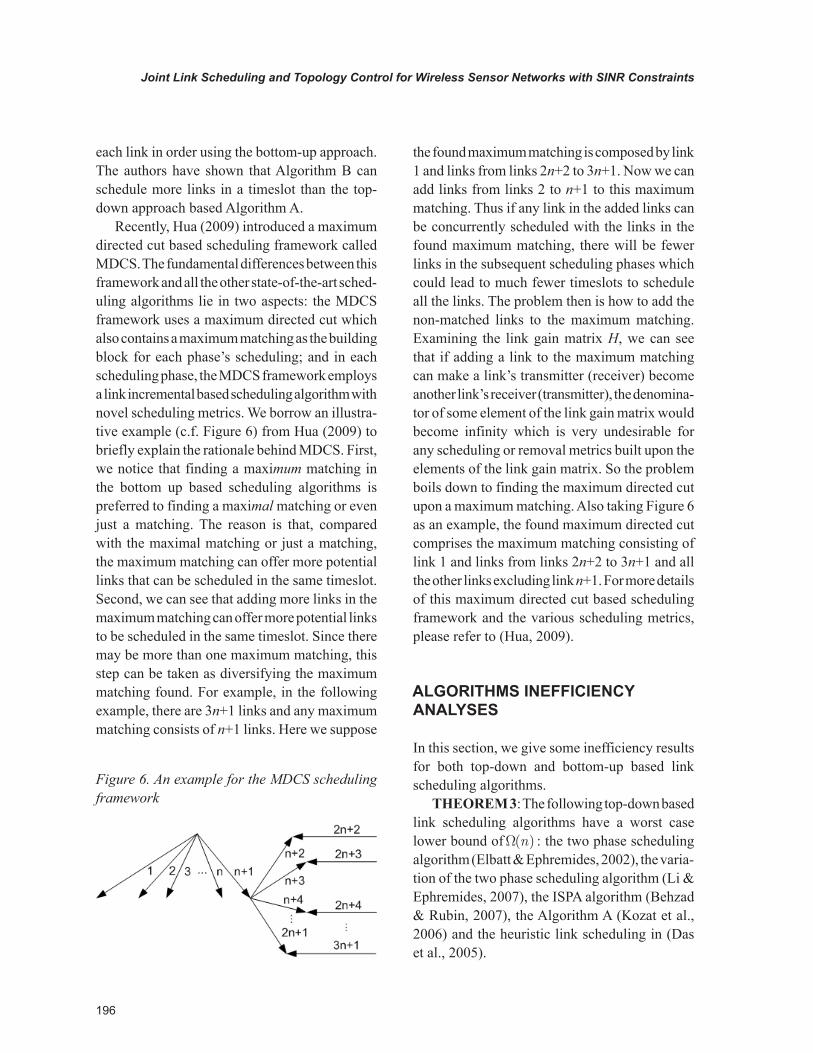
Recently, Hua (2009) introduced a maximum directed cut based scheduling framework called MDCS. The fundamental differences between this framework and all the other state-of-the-art sched-uling algorithms lie in two aspects: the MDCS framework uses a maximum directed cut which also contains a maximum matching as the building block for each phase’s scheduling; and in each scheduling phase, the MDCS framework employs a link incremental based scheduling algorithm with novel scheduling metrics. We borrow an illustra-tive example (c.f. Figure 6) from Hua (2009) to briefly explain the rationale behind MDCS. First, we notice that finding a maximum matching in the bottom up based scheduling algorithms is preferred to finding a maximal matching or even just a matching. The reason is that, compared with the maximal matching or just a matching, the maximum matching can offer more potential links that can be scheduled in the same timeslot. Second, we can see that adding more links in the maximum matching can offer more potential links to be scheduled in the same timeslot. Since there may be more than one maximum matching, this step can be taken as diversifying the maximum matching found. For example, in the following example, there are 3n+1 links and any maximum matching consists of n+1 links. Here we suppose

the found maximum matching is composed by link 1 and links from links 2n+2 to 3n+1. Now we can add links from links 2 to n+1 to this maximum matching. Thus if any link in the added links can be concurrently scheduled with the links in the found maximum matching, there will be fewer links in the subsequent scheduling phases which could lead to much fewer timeslots to schedule all the links. The problem then is how to add the non-matched links to the maximum matching. Examining the link gain matrix H, we can see that if adding a link to the maximum matching can make a link’s transmitter (receiver) become another link’s receiver (transmitter), the denomina-tor of some element of the link gain matrix would become infinity which is very undesirable for any scheduling or removal metrics built upon the elements of the link gain matrix. So the problem boils down to finding the maximum directed cut upon a maximum matching. Also taking Figure 6 as an example, the found maximum directed cut comprises the maximum matching consisting of link 1 and links from links 2n+2 to 3n+1 and all the other links excluding link n+1. For more details of this maximum directed cut based scheduling framework and the various scheduling metrics, please refer to (Hua, 2009).

ALGORITHMS INEFFICIENCY ANALYSES

In this section, we give some inefficiency results for both top-down and bottom-up based link scheduling algorithms.

THEOREM 3: The following top-down based link scheduling algorithms have a worst case lower bound ofW( )n : the two phase scheduling algorithm (Elbatt & Ephremides, 2002), the varia-tion of the two phase scheduling algorithm (Li & Ephremides, 2007), the ISPA algorithm (Behzad & Rubin, 2007), the Algorithm A (Kozat et al., 2006) and the heuristic link scheduling in (Das et al., 2005).

Figure 6. An example for the MDCS scheduling framework

197


PROOF: Since the two phase scheduling algorithm and the ISPA algorithm use LISRA and SMIRA as their link removal algorithms respectively, the inefficiency results of the two link removal algorithms (Theorem 5.2 in (Mo-scibroda, Oswald & Wattenhofer, 2007)) can be directly applied here. For the other three schedul-ing algorithms, we can make use of the co-centric exponential node chain given in Figure 5. We can set the path loss exponenta = 3 , the background noisen

i= 0 and the thresholdb = 2 . For the

variation of the two phase scheduling algorithm, since all the links have the same number of blocked links (zero), the links removed in each step are link 1 to link n-1, so only one link (link n) can be scheduled in the first timeslot. These removal steps will be repeated in the following n-1 timeslots. For the Algorithm A and the heuristic link scheduling, since they either use the link gain matrix column sum or row sum as their link removal metrics, the links removed in each step are either in an increasing order of their links’ lengths or in a decreasing order of their links’ lengths. However, both orders will result in W( )n scheduling lengths. This completes the proof.

THEOREM 4: The two bottom-up based link scheduling algorithms, i.e., the simplified sched-uling algorithm in (Li & Ephremides, 2007) and the GreedyPhysical algorithm in (Brar, Blough & Santi, 2006), have a worst case lower boundW( )n .

PROOF: We make use of the co-centric ex-ponential node chain. Since all the links form a matching, the algorithm can schedule the links in a decreasing order of their lengths. So depending on the value of maximum allowable transmission power, the corresponding power assignments can be either linear power assignments, constant power assignments, or the long links employing constant power assignments while the remaining short links would employ linear power assign-ments. By using the inefficiency results of both constant and linear power assignments (Theorem 3.1 and 3.2 in (Moscibroda & Wattenhofer, 2006))

or Theorem 4.1 in (Hua & Lau, 2006), we can complete the proof for the simplified scheduling algorithm. Similarly since the GreedyPhysical algorithm does not employ packet-level power control, which means that all the links in the same timeslot use the same transmission powers (the links in different timeslots may use different powers), Theorem 4.1 in (Hua & Lau, 2006) can be directly applied here. This completes the proof for the GreedyPhysical algorithm.

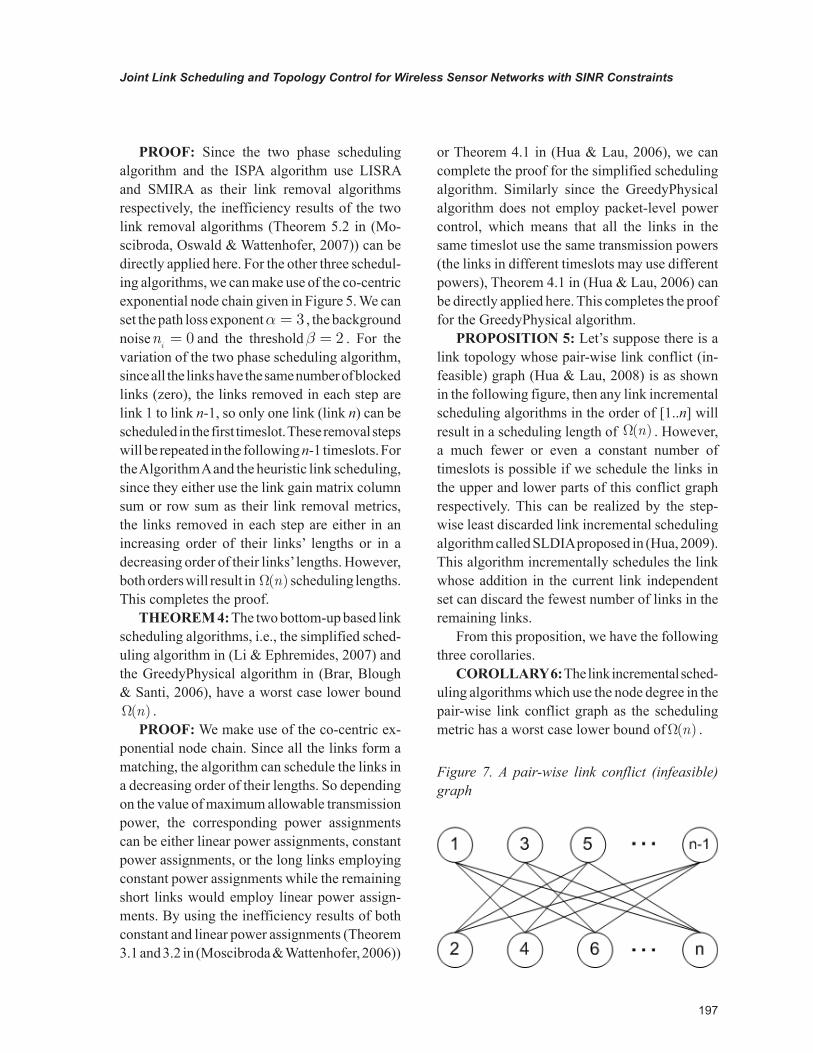
PROPOSITION 5: Let’s suppose there is a link topology whose pair-wise link conflict (in-feasible) graph (Hua & Lau, 2008) is as shown in the following figure, then any link incremental scheduling algorithms in the order of [1..n] will result in a scheduling length of W( )n . However, a much fewer or even a constant number of timeslots is possible if we schedule the links in the upper and lower parts of this conflict graph respectively. This can be realized by the step-wise least discarded link incremental scheduling algorithm called SLDIA proposed in (Hua, 2009). This algorithm incrementally schedules the link whose addition in the current link independent set can discard the fewest number of links in the remaining links.

From this proposition, we have the following three corollaries.

COROLLARY 6: The link incremental sched-uling algorithms which use the node degree in the pair-wise link conflict graph as the scheduling metric has a worst case lower bound ofW( )n .

Figure 7. A pair-wise link conflict (infeasible) graph

198


COROLLARY 7: Since all the links have unit link demand in MLSAT, the link incremental scheduling algorithms which use the link demands as a scheduling metric, such as the Primal Algo-rithm in (Borbash & Ephremides, 2006) and the IDGS algorithm in (Fu, Liew & Huang, 2008), have a worst case lower bound ofW( )n .

COROLLARY 8: Let’s further suppose all the links in this link topology have the same number of blocked links, then the link incremental schedul-ing algorithms which use the number of blocked links as the scheduling metric, such as the JSPCA algorithm in (Li & Ephremides, 2007) and the LSPC Algorithm in (Ramamurthi et al., 2008), have a worst case lower bound ofW( )n .

JOINT TOPOLOGY CONSTRUCTION AND LINK SCHEDULING FOR MLSTT

In this section, we review some joint topology construction and link scheduling algorithms for the MLSTT problem. The first algorithm for this problem is given in (Moscibroda & Wattenhofer, 2006) in the context of fulfilling the connectivity property of all the arbitrarily located nodes on the plane. If we remove the last step of this algorithm, i.e., adding the links from the sink node to all the other nodes, this algorithm can be directly used for MLSTT. Since this algorithm employs the nonlinear power assignment and is targeted for narrow band networks, we call it NPAN. The NPAN proceeds in phases, where each phase comprises all the links in the nearest neighbor forest constructed over the sink nodes of the links in the previous phase. Here the sink node means the node with no outgoing links. This scheduling algorithm partitions the links in each phase into different groups based on the links’ lengths, and then it incrementally schedules each link in the selected groups with the nonlinear power assignment. Since there areO n(log )groups in each scheduling phase (n is the number of the nodes) and there areO n(log )phases, by combin-ing the scheduling length of each group which is

bounded byO n(log )2 , the total scheduling length isO n(log )4 . In a follow-up paper (Hua & Lau, 2006), the authors have studied how the wide-band networks would affect the poly-logarithmic scheduling length. They prove that, for a wide-band network with processing gain m, the scheduling length can be reduced toO n m n(log( / ) log )× 3 . This result shows that a higher processing gain can greatly shorten the scheduling length, espe-cially whenm n= Q( ) . In addition, the paper also points out that the poly-logarithmic scheduling length is achieved at the expense of total power consumption which is an exponential function of the number of the nodes. Now if we do not schedule the links in each phase but rather to schedule the links when the tree topology has been constructed afterO n(log ) steps, the scheduling length can be reduced toO n(log )3 . This result is derived from the paper (Moscibroda, Wattenhofer & Zollinger, 2006) which proves that the schedul-ing length for arbitrary topologies is bounded by the in-interference degree of the topology times O n(log )2 , and the in-interference degree of the iteratively constructed tree topology isO n(log ) . By using a slightly different nonlinear power as-signment in (Moscibroda, 2007), the scheduling length has been further reduced toO n(log )2 . In this chapter, the algorithm first iteratively constructs the tree through the nearest component connector algorithm (Fussen, 2004) which is almost the same as the nearest forest connection algorithm. Second, the algorithm partitions all the links in constant number of groups based on the links’ lengths. The final result is reached since the scheduling length for each group isO n(log )2 . We call this schedul-ing algorithm NPAN-IPSN07. Here we take note that the results of (Hua & Lau, 2006) can be easily extended to all these follow-up nonlinear power assignment based scheduling algorithms.

Instead of iteratively connecting all the arbi-trarily located nodes with either the nearest forest connection algorithm or the nearest component connector algorithm, Hua (2009) has recently

199


proposed another joint topology construction and link scheduling algorithm based on first construct-ing a minimum spanning tree. The algorithm does not use nonlinear power assignment based scheduling algorithms but rather the proposed maximum directed cut based scheduling frame-work (MDCS).

ALGORITHM COMPARISONS

In this section, we compare the scheduling lengths generated by various link scheduling algorithms for both the MLSAT and MLSTT problems in-troduced in this chapter.

Comparisons of Algorithms for MLSAT

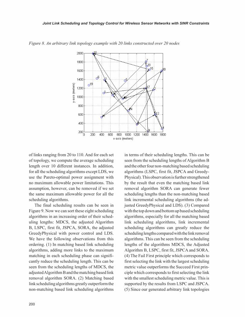
First we show how the arbitrary link topologies are generated. For any n arbitrarily located nodes in a 2000×2000 m2 plane, we randomly select a link’s transmitter and receiver subject to the con-straint that they are different nodes on the plane. We then repeat this process until a number of n different links (either with different transmitters or receivers) have been constructed. So in this topology construction some nodes may not be used (Figure 8 is an example). In this simulation, we set the path loss exponenta = 4 and the threshold b = 2 . In fact we have also tested all the schedul-ing algorithms for the other ( , )a b values. Since the arbitrarily generated link topology is a very dense link topology (c.f. Figure 8), if we choose a smallera value or a largerb value, all of the sched-uling algorithms can schedule at most one link in each timeslot which would make performance comparison impossible. However for some other( , )a b values which either have a largera value or a smallerb value, all the algorithms behave simi-larly with thea = 4 andb = 2 setting. So we only give the simulation results for the ( , )a b= =4 2case. We implemented seven bottom-up based scheduling algorithms: the MDCS scheduling

framework (Hua, 2009), the adjusted Algorithm B (Kozat, Koutsopoulos & Tassiulas, 2006), the GreedyPhysical algorithm in (Brar, Blough & Santi, 2006) with packet level power control, the JSPCA algorithm in (Li & Ephremides, 2007), the LSPC algorithm in (Ramamurthi et al., 2008), the LDS algorithm in (Moscibroda, Oswald & Wattenhofer, 2007) and the first fit based link increment scheduling algorithm. Here by first fit based link incremental scheduling algorithm, we mean that we just greedily schedule the links in its unsorted order with the bottom up approach. In addition, in order to differentiate from the JSPCA algorithm, the LSPC algorithm employs a decreasing order of the number of blocked links to incrementally schedule the links. Note that for the LDS algorithm, since its scheduling length relies on the parameterr , we have tested differentr values and find that LDS can achieve the shortest scheduling length whenr = 1 , so we setr = 1 in our simulation. We also imple-ment one top-down based scheduling algorithm which uses the link removal algorithm SORA. This algorithm first finds a maximum matching in each scheduling phase; then it employs SORA as the link removal algorithm. The reasons we use SORA as a representative for top down based link removal algorithms are: first, the simulation results in (Wu, 1999) have shown that, compared with SRA and SMIRA, SORA has the lowest out-age probability and a better throughput capacity; second, for the co-centric exponential node chain topology, our own simulation result shows that the SORA algorithm can schedule it with the number of timeslots no more than that by the nonlinear power assignment based link scheduling algorithm given in (Moscibroda, Oswald & Wattenhofer, 2007); third, compared with all the other link removal based scheduling algorithms which have worst case lower boundW( )n where n is the number of the links, the scheduling length lower bound for the SORA algorithm is still unknown. Note that, we have tested these scheduling algorithms over ten sets of link topologies with the number

200


of links ranging from 20 to 110. And for each set of topology, we compute the average scheduling length over 10 different instances. In addition, for all the scheduling algorithms except LDS, we use the Pareto-optimal power assignment with no maximum allowable power limitations. This assumption, however, can be removed if we set the same maximum allowable power for all the scheduling algorithms.

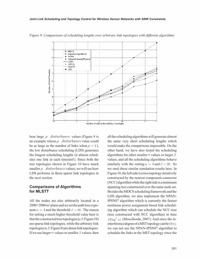
The final scheduling results can be seen in Figure 9. Now we can sort these eight scheduling algorithms in an increasing order of their sched-uling lengths: MDCS, the adjusted Algorithm B, LSPC, first fit, JSPCA, SORA, the adjusted GreedyPhysical with power control and LDS. We have the following observations from this ordering. (1) In matching based link scheduling algorithms, adding more links to the maximum matching in each scheduling phase can signifi-cantly reduce the scheduling length. This can be seen from the scheduling lengths of MDCS, the adjusted Algorithm B and the matching based link removal algorithm SORA. (2) Matching based link scheduling algorithms greatly outperform the non-matching based link scheduling algorithms

in terms of their scheduling lengths. This can be seen from the scheduling lengths of Algorithm B and the other four non-matching based scheduling algorithms (LSPC, first fit, JSPCA and Greedy-Physical). This observation is further strengthened by the result that even the matching based link removal algorithm SORA can generate fewer scheduling lengths than the non-matching based link incremental scheduling algorithms (the ad-justed GreedyPhysical and LDS). (3) Compared with the top down and bottom up based scheduling algorithms, especially for all the matching based link scheduling algorithms, link incremental scheduling algorithms can greatly reduce the scheduling lengths compared with the link removal algorithms. This can be seen from the scheduling lengths of the algorithms MDCS, the Adjusted Algorithm B, LSPC, first fit, JSPCA and SORA. (4) The Fail First principle which corresponds to first selecting the link with the largest scheduling metric value outperforms the Succeed First prin-ciple which corresponds to first selecting the link with the smallest scheduling metric value. This is supported by the results from LSPC and JSPCA. (5) Since our generated arbitrary link topologies

Figure 8. An arbitrary link topology example with 20 links constructed over 20 nodes

201


bear large r -disturbance values (Figure 8 is an example whoser -disturbance value could be as large as the number of links whenr = 1 ), the low disturbance scheduling (LDS) generates the longest scheduling lengths (it almost sched-ules one link in each timeslot!). Since both the tree topologies shown in Figure 10 have much smallerr -disturbance values, we will see how LDS performs in these sparse link topologies in the next section.

Comparisons of Algorithms for MLSTT

All the nodes are also arbitrarily located in a 2000×2000 m2 plane and we set the path loss expo-nenta = 4 and the thresholdb = 20 . The reason for setting a much higher threshold value here is that the constructed tree topologies (c.f. Figure 10) are sparse link topologies, while the arbitrary link topologies (c.f. Figure 8) are dense link topologies. If we use largera values or smallerb values, then

all the scheduling algorithms will generate almost the same very short scheduling lengths which would make the comparisons impossible. On the other hand, we have also tested the scheduling algorithms for other smallera values or largerbvalues, and all the scheduling algorithms behave similarly with the settinga = 4 andb = 20 . So we omit these similar simulation results here. In Figure 10, the left side is a tree topology iteratively constructed by the nearest component connector (NCC) algorithm while the right side is a minimum spanning tree constructed over the same node set. Besides the MDCS scheduling framework and the LDS algorithm, we also implement the NPAN-IPSN07 algorithm which is currently the fastest nonlinear power assignment based link schedul-ing algorithm which can schedule the NCC-tree (tree constructed with NCC algorithm) in timeO n(log )2 (Mosciborda, 2007). And since the in-interference degree of a MST topology can beO n( ) we can not use the NPAN-IPSN07 algorithm to schedule the links in the MST topology since the

Figure 9. Comparisons of scheduling lengths over arbitrary link topologies with different algorithms

202


SINR constraints may not be satisfied. So for the MST topology, we apply the MDCS and the LDS scheduling algorithms, and for the NCC tree, we can also apply the NPAN-IPSN07 algorithm. But for the NPAN-IPSN07 algorithm, we must pay attention to the background noise valueni since the scheduling length is also dependent on this parameter. Note that, in this algorithm, when the background noiseni < - × -( ) / ( ( ))a b a2 2 1 the SINR constraints can not be guaranteed by the proposed nonlinear power assignment (the reason is that the SNR model must be satisfied). So in this simulation, we set all theni to have the same value which is a little bit larger than( ) / ( ( ))a b a- × -2 2 1 since we have found that a much largerni value can greatly increase the scheduling length.

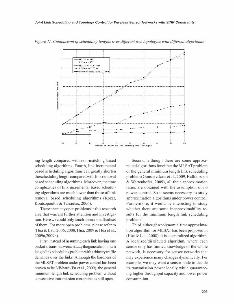
The scheduling results are shown in Figure 11. From this figure we have the following ob-servations: (1) the MST topology always yields much shorter scheduling lengths no matter which scheduling algorithm is used; (2) combined with Figure 4, for the MST and NCC tree topologies having much lowerr -disturbance values, LDS generates shorter scheduling lengths; although the reduction is not that significant, the reduction of

scheduling lengths with MDCS is huge; (3) for both MST and NCC tree topologies, the MDCS algorithm always achieves the shortest schedul-ing lengths; (4) for NCC tree, compared with the NPAN-IPSN07 algorithm, MDCS achieves a much shorter scheduling length.

CONCLUSION

This chapter reviews all the state-of-the-art poly-nomial time link scheduling algorithms under the SINR model. We have studied these algorithms through theoretical analyses as well as using simulation. We can draw some conclusions from the results. First, for both dense and sparse link topologies, the maximum directed cut based sched-uling framework MDCS significantly outperforms all the other state-of-the-art link scheduling algo-rithms in terms of scheduling length. Second, our results show that connecting all the nodes (sensors) on a plane with the minimum spanning tree topol-ogy can greatly shorten the scheduling lengths, which means that the data gathering speed can be significantly increased. Third, matching based scheduling algorithms help reduce the schedul-

Figure 10. Different tree topologies over the same set of nodes (Left: iterative nearest component con-nector construction; Right: minimum spanning tree construction)

203


ing length compared with non-matching based scheduling algorithms. Fourth, link incremental based scheduling algorithms can greatly shorten the scheduling length compared with link removal based scheduling algorithms. Moreover, the time complexities of link incremental based schedul-ing algorithms are much lower than those of link removal based scheduling algorithms (Kozat, Koutsopoulos & Tassiulas, 2006).

There are many open problems in this research area that warrant further attention and investiga-tion. Here we could only touch upon a small subset of them. For more open problems, please refer to (Hua & Lau, 2006, 2008, Hua, 2009 & Hua et al., 2009a,2009b).

First, instead of assuming each link having one packet to transmit, we can study the general minimum length link scheduling problem with arbitrary traffic demands over the links. Although the hardness of the MLSAT problem under power control has been proven to be NP-hard (Fu et al., 2009), the general minimum length link scheduling problem without consecutive transmission constraints is still open.

Second, although there are some approxi-mated algorithms for either the MLSAT problem or the general minimum length link scheduling problem (Goussevskaia et al., 2009, Halldorsson & Wattenhofer, 2009), all their approximation ratios are obtained with the assumption of no power control. So it seems necessary to study approximation algorithms under power control. Furthermore, it would be interesting to study whether there are some inapproximability re-sults for the minimum length link scheduling problems.

Third, although a polynomial time approxima-tion algorithm for MLSAT has been proposed in (Hua & Lau, 2008), it is a centralized algorithm. A localized/distributed algorithm, where each sensor only has limited knowledge of the whole network, is necessary for sensor networks that may experience many changes dynamically. For example, we may want a sensor node to decide its transmission power locally while guarantee-ing higher throughput capacity and lower power consumption.

Figure 11. Comparison of scheduling lengths over different tree topologies with different algorithms

204


Fourth, for the asymptotic upper bound of the scheduling length of the MLSTT problem, our simulation results and analyses have shown that the currently fastest O n(log )2 bound (Moscibroda, 2007) can be further reduced, which needs a novel scheduling algorithm. Moreover, a non-trivial lower bound is also needed.

Fifth, it will be interesting to consider more layers of the sensor networks, such as the network-ing layer. For example, a joint link scheduling, topology control and routing solution with a much shorter provable scheduling length can be very challenging (Chafekar et al., 2007).

Sixth, it will also be interesting to consider other joint link scheduling and topology control problems. For example, we can consider the minimum frame length link scheduling problem for either a k-connected topology or a t-spanner topology.

Seventh, for a small number of links, it is pos-sible to design some efficient exact algorithms for either the MLSAT or the general minimum length link scheduling problems. These problems can be formulated as a set covering problem (Hua & Lau, 2008) or as a set multi-covering problem (Hua et al., 2009a, 2009b).

Finally, it should be worthwhile to take the packets’ arriving rates into account (i.e., stochas-tic network) when trying to solve the joint link scheduling and topology control problems (Joo, Lin & Shroff, 2008).

ACKNOWLEDGMENT

This research is supported in part by a Hong Kong RGC-GRF grant (7136/07E), the national 863 high-tech R&D program of the Ministry of Science and Technology of China under grant No. 2006AA10Z216, the National Science Founda-tion of China under grant No. 60604033, and the National Basic Research Program of China Grant 2007CB807900, 2007CB807901.

REFERENCES

Andersin, M., Rosberg, Z., & Zander, J. (1996). Gradual removals in cellular PCS with constrained power control and noise. Wireless Networks, 2(1), 27–43. doi:10.1007/BF01201460

Baccelli, F., Bambos, N., & Chan, C. (2006). Op-timal Power, Throughput and Routing for Wireless Link Arrays. In 25th IEEE International Conference on Computer Communications, Joint Conference of the IEEE Computer and Communications Societies (INFOCOM). Barcelona, Spain: IEEE.

Behzad, A., & Rubin, I. (2007). Optimum in-tegrated link scheduling and power control for multihop wireless networks. IEEE Transac-tions on Vehicular Technology, 56(1), 194–205. doi:10.1109/TVT.2006.883734

Borbash, S. A., & Ephremides, A. (2006). Wire-less link scheduling with power control and SINR constraints. IEEE Transactions on Infor-mation Theory, 52(11), 5106–5111. doi:10.1109/TIT.2006.883617

Brar, G., Blough, D., & Santi, P. (2006). Compu-tationally efficient scheduling with the physical interference model for throughput improvement in wireless mesh networks. In M. Gerla, C. Petrioli, & R. Ramjee (Ed.), Proceedings of the 12th annual international conference on Mobile computing and networking (MOBICOM) (pp.2-13). Los Angeles: ACM.

Burkhart, M., Rickenbach, P., von Wattenhofer, R., & Zollinger, A. (2004). Does Topology Control Reduce Interference? In J. Murai, C. E. Perkins, & L. Tassiulas (Eds.), Proceedings of the 5th ACM Interational Symposium on Mobile Ad Hoc Networking and Computing (MOBIHOC) (pp.9-19).Tokyo: ACM.

205


Chafekar, D., Kumar, V. S., Marathe, M., Parthasarathy, S., & Srinivasan, A. (2007). Cross-layer latency minimization for wireless networks using SINR constraints. In E. Kranakis, E. M. Belding, & E. Modiano (Eds.), Proceedings of the 8th ACM Interational Symposium on Mobile Ad Hoc Networking and Computing (MOBIHOC) (pp.110-119). Montreal, Quebec: ACM.

Das, A. K., Marks, R. J., II, Arabshahi, P., & Gray, A. (2005). Power controlled minimum frame length scheduling in TDMA wireless networks with sectored antennas. In 24th IEEE International Conference on Computer Communications, Joint Conference of the IEEE Computer and Com-munications Societies (INFOCOM). Miami, FL: IEEE.

ElBatt, T., & Ephremides, A. (2002). Joint sched-uling and power control for wireless ad-hoc net-works. In 21st IEEE International Conference on Computer Communications, Joint Conference of the IEEE Computer and Communications Societ-ies (INFOCOM). New York: IEEE.

Fu, L., Liew, S., & Huang, J. (2008). Joint power control and link scheduling in wireless networks for throughput optimization. In Proceedings IEEE ICC. Beijing, China: IEEE.

Fu, L., Liew, S., & Huang, J. (2009). Power con-trolled scheduling with consecutive transmission constraints: complexity analysis and algorithm design. In 28th IEEE International Conference on Computer Communications, Joint Conference of the IEEE Computer and Communications Societ-ies (INFOCOM). Rio de Janeiro, Brazil: IEEE.

Fussen, M. (2004). Sensor networks: interference reduction and possible applications. Diploma Thesis, Distributed Computing Group, ETH Zurich, Switzerland.

Gao, Y., Hou, J. C., & Nguyen, H. (2008). Topology control for maintaining network connectivity and maximizing network capacity under the physical model. In 27th IEEE International Conference on Computer Communications, Joint Conference of the IEEE Computer and Communications Societ-ies (INFOCOM). Phoenix, AZ: IEEE.

Goldsmith, A. J., & Wicker, S. B. (2002). Design challenges for energy-constrained ad hoc wireless networks. IEEE Wireless Communications, 9(4), 8–27. doi:10.1109/MWC.2002.1028874

Goussevskaia, O., Halldorsson, M., Wattenhofer, R., & Welzl, E. (2009). Capacity of arbitrary wireless networks. In 28th IEEE International Conference on Computer Communications, Joint Conference of the IEEE Computer and Commu-nications Societies (INFOCOM). Rio de Janeiro, Brazil: IEEE.

Goussevskaia, O., Oswald, Y. A., & Wattenhofer, R. (2007). Complexity in geometric SINR. In E. Kranakis, E. M. Belding, & E. Modiano (Eds.), Proceedings of the 8th ACM Interational Symposium on Mobile Ad Hoc Networking and Computing (MOBIHOC) (pp.110-119). Montreal, Quebec: ACM.

Gupta, P., & Kumar, P. R. (2000). The capac-ity of wireless networks. IEEE Transactions on Information Theory, 46(2), 388–404. doi:10.1109/18.825799

Hajek, B. E., & Sasaki, G. H. (1988). Link scheduling in polynomial time. IEEE Transac-tions on Information Theory, 34(5), 910–917. doi:10.1109/18.21215

Halldorsson, M., & Wattenhofer, R. (2009). Wireless communication is in APX. In 36th In-ternational Colloquium on Automata, Languages and Programming (ICALP), Rhodes, Greece: Springer-Verlag.

206


Hua, Q.-S. (2009). Scheduling wireless links with SINR constraints. PhD Thesis, The University of Hong Kong.

Hua, Q.-S., & Lau, F. C. M. (2006). The scheduling and energy complexity of strong connectivity in ultra-wideband networks. In E. Alba, C.-F. Chias-serini, N. B. Abu-Ghazaleh, & R. Lo Cigno (Eds.), Proceedings of the 9th International Symposium on Modeling Analysis and Simulation of Wireless and Mobile Systems (MSWiM) (pp.282-290). Ter-romolinos, Spain: ACM.

Hua, Q.-S., & Lau, F. C. M. (2008). Exact and approximate link scheduling algorithms under the physical interference model. In M. Segal, & A. Kesselman (Eds.), Proceedings of the DIALM-POMC Joint Workshop on Foundations of Mobile Computing (pp.45-54). Toronto, Canada: ACM.

Hua, Q.-S., Wang, Y., Yu, D., & Lau, F. C. M. (2009a). Set multi-covering via Inclusion-Exclu-sion. Theoretical Computer Science, 410(38-40), 3882–3892. doi:10.1016/j.tcs.2009.05.020

Hua, Q.-S., Yu, D., Lau, F. C. M., & Wang, Y. (2009b). Exact algorithms for set multicover and multiset multicover problems. In Y. Dong, D.-Z. Du, O. H. Ibarra (Eds.), Proceedings of the 20th International Symposium on Algorithms and Com-putation (ISAAC) (pp. 34-44). Hawaii: Springer.

Joo, C., Lin, X., & Shroff, N. B. (2008). Under-standing the capacity region of the greedy maximal scheduling algorithm in multi-hop wireless net-works. In 27th IEEE International Conference on Computer Communications, Joint Conference of the IEEE Computer and Communications Societ-ies (INFOCOM). Phoenix, AZ: IEEE.

Kozat, U. C., Koutsopoulos, I., & Tassiulas, L. (2006). Cross-layer design for power efficiency and QoS provisioning in multi-hop wireless networks. IEEE Transactions on Wireless Com-munications, 5(11), 3306–3315. doi:10.1109/TWC.2006.05058

Lee, T. H., Lin, J. C., & Su, Y. T. (1995). Downlink power control algorithms for cellular radio sys-tems. IEEE Transactions on Vehicular Technology, 44(1), 89–94. doi:10.1109/25.350273

Li, Y., & Ephremides, A. (2007). A joint schedul-ing, power control, and routing algorithm for ad hoc wireless networks. Ad Hoc Networks, 5(7), 959–973. doi:10.1016/j.adhoc.2006.04.005

Locher, T., von Rickenbach, P., & Wattenhofer, R. (2008). Sensor networks continue to puzzle: selected open problems. In S. Rao, M. Chatterjee, P. Jayanti, C. S. R. Murthy, & S. K. Saha (Eds.): 9th International Conference on Distributed Computing and Networking (ICDCN) (pp.25-38). Kolkata, India: Springer.

Moscibroda, T. (2007). The worst-case capacity of wireless sensor networks. In T. F. Abdelzaher, L. J. Guibas, & M. Welsh (Eds.), Proceedings of the 6th International Conference on Information Processing in Sensor Networks (IPSN) (pp.1-10). Cambridge, MA: ACM.

Moscibroda, T., Oswald, Y. A., & Wattenhofer, R. (2007). How optimal are wireless scheduling protocols? In 26th IEEE International Conference on Computer Communications, Joint Conference of the IEEE Computer and Communications So-cieties (INFOCOM)(pp. 1433-1441). Anchorage, AK: IEEE.

Moscibroda, T., & Wattenhofer, R. (2006). The complexity of connectivity in wireless networks. In 25th IEEE International Conference on Com-puter Communications, Joint Conference of the IEEE Computer and Communications Societies (INFOCOM). Barcelona, Spain: IEEE.

Moscibroda, T., Wattenhofer, R., & Weber, Y. (2006). Protocol design beyond graph-based models. In Proceedings 5th Workshop on Hot Topics in Networks (HotNets-V) (pp.25-30). Irvine,California: ACM.

207


Moscibroda, T., Wattenhofer, R., & Zollinger, A. (2006). Topology control meets SINR: the scheduling complexity of arbitrary topologies. In S. Palazzo, M. Conti, & R. Sivakumar (Eds.), Proceedings of the 7th ACM International Symposium on Mobile Ad Hoc Networking and Computing (MOBIHOC) (pp.310-321). Florence, Italy: ACM.

Pan, V. Y., & Chen, Z. Q. (1999). The complex-ity of the matrix eigenproblem. In Proceedings of the 31st Annual ACM Symposium on Theory of Computing (STOC) (pp. 507-516). Atlanta, GA: ACM.

Pillai, S. U., Suel, T., & Cha, S. (2005). The perron-frobenius theorem and some of its applications. IEEE Signal Processing Magazine, 22(2), 62–75. doi:10.1109/MSP.2005.1406483

Ramamurthi, V., Reaz, A. S., Dixit, S., & Mukher-jee, B. (2008). Link scheduling and power con-trol in wireless mesh networks with directional antennas. In Proceedings IEEE ICC. Beijing, China: IEEE.

Santi, P. (2005). Topology control in wireless ad hoc and sensor networks. Chichester, UK: John Wiley and Sons.

Schmid, S., & Wattenhofer, R. (2006). Algorithmic models for sensor networks. In Proceedings 20th International Parallel and Distributed Process-ing Symposium (IPDPS). Rhodes Island, Greece: IEEE.

Tang, J., Xue, G., Chandler, C., & Zhang, W. (2006). Link scheduling with power control for throughput enhancement in multi-hop wire-less networks. IEEE Transactions on Vehicular Technology, 55(3), 733–742. doi:10.1109/TVT.2006.873836

Völker, M., Katz, B., & Wagner, D. (2009). On the complexity of scheduling with power control in geometric SINR. Technical Report 15, ITI Wagner, Faculty of Informatics, Universität Karlsruhe.

Wang, K., Chiasserini, C.-F., Rao, R. R., & Proa-kis, J. G. (2005). A joint solution to scheduling and power control for multicasting in wireless ad hoc networks. EURASIP Journal on Applied Signal Processing, (1): 144–152. doi:10.1155/ASP.2005.144

Wang, Y., & Li, X.-Y. (2003). Localized con-struction of bounded degree planar spanner for wireless ad hoc networks. In Proceedings of the DIALM-POMC Joint Workshop on Foundations of Mobile Computing (pp.59-68). San Diego, CA: ACM.

Wattenhofer, R., Li, L., Bahl, P., & Wang, Y.-M. (2001). Distributed topology control for power efficient operation in multihop wireless ad hoc networks. In 20th IEEE International Conference on Computer Communications, Joint Conference of the IEEE Computer and Communications So-cieties (INFOCOM)(pp. 1388-1397). Anchorage, AK: IEEE.

Wu, Q. (1999). Performance of optimum transmit-ter power control in CDMA cellular mobile sys-tems. IEEE Transactions on Vehicular Technology, 48(2), 571–575. doi:10.1109/25.752582

Zander, J. (1992a). Performance of optimum transmitter power control in cellular radio systems. IEEE Transactions on Vehicular Technology, 41(1), 57–62. doi:10.1109/25.120145

Zander, J. (1992b). Distributed cochannel inter-ference control in cellular radio systems. IEEE Transactions on Vehicular Technology, 41(3), 305–311. doi:10.1109/25.155977

KEY TERMS AND DEFINITIONS

Constant (Uniform) Power Assignment: If all the concurrently scheduled links employ the same transmission power, we call it a constant (uniform) power assignment.

208


Length Diversity: A notion to describe the number of magnitudes of lengths in a set of linksN n= { ,..., }1 . In particular, the length diversity ofN is: d N m i N d mii( ) | { | : log( ) } |= $ Î ê

ëêúûú =

is the length of link i)Linear Power Assignment: If each link in

the concurrently scheduled links employs the transmission power which is proportional to the corresponding link’s length (the distance from the transmitter to the receiver) to the power of the path loss exponent, we call it a linear power assignment.

Link Independent Set: A set of links which can be concurrently scheduled under the SINR model.

Nonlinear Power Assignment: We used i({ })to denote the length diversity of all the links{ }ischeduled in the same timeslot. And we sort the links in a non-increasing order of their lengths. Then we assign the t value (the power scaling exponent) to each link (1£ £t d i({ }) ), and the lower the length magnitude of the links, the higher the t value. In particular, the links with the lowest length magnitude have the highest tvalue ofd i({ }) , and the links with the highest length magnitude have the lowest t value of 1. Then if the link i uses the transmission powerp f diii = ×( ) ( )t a , we say it is a nonlinear power

assignment. Here f is a function of the parametersa ,b ,ni and the number of the links.

Pareto-Optimal Power Assignment: Accord-ing to Property 4 of the link gain matrix H, if we set the transmission powers based on the power vectorP I H* ( )= - ×-1 h , we call it a Pareto-optimal power assignment.

SINR Model: A specific interference model which is dependent on the so called signal-to-interference-plus-noise-ratio (SINR). In this model, we say that a link i has been successfully scheduled if and only if the power received by the link’s receiver ir from its corresponding transmit-ter is is at least a factorb higher than the sum of the received powers from the other concurrently scheduled links’ transmitters plus the background noiseni . Here the received power attenuates with distance, i.e., it equals to the transmitted power divided by the distance between the sender and receiver to the power of the path loss exponenta .

Topology Control: Adjustment of the links’ transmission powers so that these links fulfill a network-wide property, such as connectivity, low interference and capacity improvement.

Wireless Link: A wireless transmission comprised by a source node (transmitter) and a destination node (receiver).

Handbook of Research on Developments and Trends …i.cs.hku.hk/~fcmlau/papers/Chap9.pdfHandbook of...

Documents

Transcript of Handbook of Research on Developments and Trends …i.cs.hku.hk/~fcmlau/papers/Chap9.pdfHandbook of...