Handbook of Pneumatic Conveying Engineeringnguyen.hong.hai.free.fr/EBOOKS/SCIENCE AND... · 448...

16Quick Check Design Methods

1 INTRODUCTION

The design of pneumatic conveying systems is usually carried out on the basis ofscaling data obtained from the pneumatic conveying of the material to be trans-ported. If previous experience of conveying a given material is not available, datais generally derived for the purpose by conveying the material through a test facil-ity, as discussed in detail in the previous chapter. Most manufacturers of pneu-matic conveying systems have such test facilities for this purpose.

If it is required to make a quick check on the potential of an existing system,or to provide a check on design proposals, there is little information readily avail-able for the engineer to use. Pneumatic conveying does not lend itself to simplemathematical analysis, and it is l ikely that many engineers would not be able toundertake such a task easily, particularly if it were a low velocity dense phase sys-tem.

Since pneumatic conveying systems tend to have high power ratings, particu-larly for conveying in dilute phase suspension flow, it is useful to be able to obtaina rough estimate of air requirements at the feasibility stage of a project. Most of theoperating cost of a pneumatic conveying system is in the drive for the air mover. Ifan estimate can be made of the system air requirements, it is a simple matter toevaluate the operating cost in Cents per ton conveyed to see if it is at an acceptablelevel before proceeding further.

Copyright 2004 by Marcel Dekker, Inc. All Rights Reserved.

448 Chapter 16

1.1 Methods Presented

A number of straightforward methods are presented that wi l l allow a check to bemade on the design of a pneumatic conveying system in a very short space of time,whether for a new or an existing system. Horizontal and vertical sections of pipe-l ine and bends can all be accommodated, as well as dilute and dense phase convey-ing in some cases. For high pressure systems the influence of stepped pipelines canalso be incorporated.

Three different methods are presented. One is based on the value of the aironly pressure drop for the pipeline, but this is strictly limited to dilute phase con-veying only. Another is based on the use of a universal set of conveying character-istics and the third uses the steady flow energy equation as a basis. Both of thesecan be used for di lute and dense phase conveying.

1.2 Potential Accuracy

It must be emphasized that all three of these methods are strictly quick checkmethods and will provide only a first approximation solution. Although some ofthe methods may appear to be mathematically correct, do not be lulled into a falsesense of security. There is no reference to conveyed material anywhere in any ofthe procedures. In this respect reference to Figures 4.16 and 4.18 will bring anyengineer back to reality with regard to the potential accuracy of these methods,whether for dilute or dense phase conveying.

For a given material to be conveyed it is possible that the accuracy of someof these quick check methods could be improved quite considerably. If conveyingdata is available for a particular material, fine tuning could be undertaken. Con-stants relating to individual pipel ine features such as bends, vertical lift and pipe-line bore could be changed or added. Once again it must be emphasized that theresulting models would only provide more reliable system design and checkinginformation for the material being considered, and only for that particular grade ofthe material.

2 AIR ONLY PRESSURE DROP METHOD

This method uses the value of the air only pressure drop for a pipeline as a basis forevaluating its conveying potential. This resistance due to the air is related to theadditional resistance resulting from the conveying of material. The pressure dropdue to the air can be readily measured, or simply calculated for any pipeline bymeans of the equations presented in Chapter 6.

2.1 Basic Equations

The Ideal Gas Law relates the volumetric flow rate of the air to the pressure andtemperature of the air, as considered in Chapter 5. The volumetric flow rate canalso be expressed in terms of the conveying line inlet air velocity and the pipeline


Quick Check Methods 449

bore. In most conveying situations the volume occupied by the conveyed materialcan be neglected in comparison with that of the air.

These models, therefore, can be used quite reliably in gas-solid flow situa-tions. Material flow rate can be introduced in terms of the solids loading ratio ofthe conveyed material. The solids loading ratio is a parameter that is often knownapproximately, and in these cases quite simple equations can be derived equatingthe variables.

2. /. / Solids Loading Ratio

Solids loading ratio, $, is defined as the ratio of the mass flow rate of the materialconveyed, to the mass flow rate of the air used to convey the material and this wasfirst presented at Equation 4.5:

m(j) = (dimensionless) - - - - - - - (])

m

where «„ = mass flow rate of material - Ib/h

and ma = mass flow rate of air - Ib/h

It is a dimensionless ratio and is a particularly useful parameter since itsvalue remains constant along the length of a pipeline, regardless of the air pressureand conveying air velocity.

2.7.2 Ideal Gas Law

Air mass flow rate is not always a convenient parameter with which to work, andair flow rate is more usually expressed in volumetric terms. From the Ideal GasLaw, for a steady flow situation, however, one can readily be evaluated from theother, as first illustrated at Equation 5.4:

144 p V = ma R T - - - - - - - - - - - - (2)

where p = absolute pressure of gas - Ibf/in2

V = volumetric flow rate ofgas at pressure ;P - fVYmin

ma = mass flow rate of gas - Ib/min

R = characteristic gas constant - ft Ibf/lb Rand T = absolute temperature of gas - R

= / °F + 460


450 Chapter 16

2.1.3 Volumetric Flow Rate

Volumetric flow rate is given by:

V = velocity * area

and for a circular pipe

n d2

576ft'/min - - - - - - (3)

where C = conveying air velocity - ft/minand d = pipe bore - in

This is the actual volumetric flow rate. Since air and other gases are com-pressible, volumetric flow rate will change with both pressure and temperature. Italso means that the conveying air velocity wi l l vary along the length of a pipeline.A full explanation and analysis of this was included in Chapter 5 on Air Require-ments.

2.2 Working Relationships

The three equations presented above are exact equations, and so any combinationof these equations will similarly produce precise relationships. Although theseequations include all the basic parameters in pneumatic conveying, they will notproduce design relationships. This is because they do not include the necessaryfundamental relationships between material flow rate, pressure drop and conveyingair velocity. Combinations of Equations 1 to 3, however, wi l l produce equationsthat can be usefully used to check system designs. They wil l also provide a goodbasis for the inclusion of design relationships.

2.2.1 Material Flow Rate

By substituting Equation 3 into 2 to eliminate V , making ma the subject of the

equation and substituting this into Equation 1 gives:

9n d p C

mn = <p x x ib/hp 4 RT

By putting R = 53-3 ft Ibf/lb R for air gives:

r /2p C dmn = 6 x ib/h - - - - - - - ( 4 )

P v 61.9T



2.2.2 Pipeline Bore

For a given material flow rate and conveying conditions, the diameter of the pipe-line is generally required. An alternative arrangement of the equations gives:

nO-5T

d = 8'24' P

1P

2.2.3 Conveying Line Pressure Drop

An alternative arrangement, in terms of the pressure required to convey the mate-rial gives:

mp Tp = 67-9 —-^— Ibf/in2 abs - - - - - (6 )

C dz 6

2.2.3.1 Reference ConditionsThe variables in these equations can be taken at any point along the pipeline. Inthe case of air pressure and velocity, however, these are generally only known,with any degree of accuracy, at the very start and end of a pipeline. Since the con-veying line inlet air velocity is probably the most critical parameter in system de-sign it is generally conditions at the material feed point, at the start of the pipeline,that are used for this purpose.

2.3 Empirical Relationships

It will be seen from Equations 4 to 6 that, for a given material and pipeline, thereare six variables relating the main conveying parameters. Of these, the conveyingair temperature wil l be known; solids loading ratio is a function of the conveyingair velocity, pipeline bore and material flow rate; and either the material flow raterequired, pipeline bore to be used, or conveying l ine pressure drop available willbe specified. This means that there are three basic variables in each of these equa-tions.

It wi l l be possible to provide solutions to Equations 4 to 6, therefore, if twofurther relationships can be provided. These wil l , by necessity, be empirical, andso the accuracy of any expressions developed wi l l ultimately depend upon theaccuracy of the empirical relationships used. The first of these is a relationship orsuggested value for conveying line inlet air velocity. The second is a relationshipfor solids loading ratio and this is in terms of conveying line pressure drop pa-rameters.


452 Chapter 16

2.3.1 Conveying Line Inlet Air Velocity

The conveying line inlet air velocity to be employed depends upon the min imumconveying air velocity at which the material can be successfully conveyed. Thisdepends very much upon the material to be conveyed and the solids loading ratioat which it is to be conveyed.

A graphical representation of this relationship between minimum conveyingair velocity and solids loading ratio for typical powdered and granular materials ispresented in Figure 16.1. These relationships for different materials were first in-troduced in Chapter 4.

For a material that is capable of being conveyed in dense phase, such as amaterial having good air retention properties like barite, fine fly ash or cement, theconveying limits are defined approximately by:

Cmin = 2300 for ^ < 10

Cmin = (7330 $T°-3 - 1370) for 10 < </> < 80 ft/min - -

Cmin = 600 for <f> > 80

where Cmm = minimum conveying air velocity - ft/minand <b = solids loading ratio - -

(7)

3000

2000>

g 1000u

Material having dilute phaseconveying capability only

Material with dense phaseconveying capability

20 40 60

Solids Loading Ratio

80 100

Figure 16.1 Relationship between min imum conveying air velocity and solids loadingratio for different materials.



For a material that is not capable of being conveyed in dense phase, such asgranular materials having both poor air retention and poor permeability, the con-veying limits are defined approximately by:

Cmm = 2300 to 3200 ft/min (for all (8)

A graphical representation, for typical materials, of these relationships be-tween minimum conveying air velocity and solids loading ratio is also included onFigure 16.1. For most purposes, the use of this graph probably provides the quick-est means of determining the necessary value, but for anyone wanting to programthe analysis, Equations 7 and 8 are offered for this purpose.

Design would generally be based on a conveying line inlet air velocity, C/,20% greater than the min imum conveying air velocity, C,,,,,,:

C, = 1-2 ft/min (9)

2.3.2 Solids Loading Ratio

An approximate relationship between pressure drop and solids loading ratio, fordilute phase conveying, is presented in Figure 16.2. The relationship is based uponthe assumption that the curves on Figure 16.2 are equi-spaced with respect to con-veying line pressure drop. For many materials conveyed in dilute phase this is areasonable approximation.

Air Flow Rate - V0

Figure 16.2 Influence of solids loading ratio and air flow rate on conveying line pres-sure drop for d i lu te phase suspension How.


454 Chapter 16

A mathematical expression for this is:

(10)

where Apc

and Ap,,

2.3.3 Material Flow Rale

Now from Equation I :

conveying line pressure drop - Ibf/irTair only pressure drop - Ibf/in2

mPm.

Directly equating these two expressions for solids loading ratio gives:

mp = Ib/h (11)

If air mass flow rate, ma , is not a convenient parameter, Equation 11 can be

expressed in an alternative form, in terms of air pressure, p, and velocity, C, bysubstituting a combination of Equations 3 and 5 to give:

mP

p n d C

4 R TIb/h

Another alternative is to substitute solids loading ratio, </>, from Equation 10into Equation 4, which gives:

mp =p C d2

67-9 TIb/h (12)

Pipeline inlet conditions are the most convenient to use here.

2.3.3.1 Negative Pressure SystemsFor vacuum systems the pressure, p, wil l be atmospheric.



2.3.3.2 Positive Pressure SystemsFor positive pressure systems the pressure, p, in Equation 12 w i l l be equal to theconveying line pressure drop, A/?c, plus atmospheric pressure, which is:

where A/? r= conveying line pressure drop - lbf/in2

and paln, = atmospheric pressure - lbf/in2

2. 3. 4 Pipeline Bore

By substituting the solids loading ratio, (/), from Equation 10 into Equation 5, theexpression can be in terms of the pipeline bore required:

d = 8-24A/?,,

Pin (13)

The situation for both positive and negative pressure systems is the same asabove.

2.3.5 A ir Supply Pressure

Alternatively, the expression can be in terms of the pressure required to convey the

material. Substituting the solids loading ratio, 0, from Equation 10 into Equation 6gives:

p = 67-9T

C d'lbf/in2 abs - (14)

Pipeline inlet conditions are again the most convenient to use.

2.3.5.1 Negative Pressure SystemsFor negative pressure systems the pressure, p, wi l l be atmospheric and hence Apc

can be determined, which is the value required in this case. Re-arranging Equation14 and expressing in terms of pipeline inlet conditions for this case gives:

67-9md~

.+ 1 | lbf/in2

(15)


456 Chapter 16

2.3.5.2 Positive Pressure SystemsFor a positive pressure system:

A/7C = Pa,

Substituting this into Equation 14 and expressing in terms of pipeline in le tconditions gives:

PllPl = 67'9

mp

This is a quadratic equation, the solution to which is:

P Palm \Patm2 212mpTl&pa

(16)

Note:This wi l l give the correct root.

2.3.6 Air Only Pressure Drop

Since the air only pressure drop, Apa, features prominently in all of these models,a convenient expression for this pressure drop is required. An expression that willgive the air only pressure drop in terms of conveying line inlet, or exit, air velocityis needed. These models were derived in detail in Chapter 6 on The Air Only Da-tum.

2.3.6.1 Negative Pressure SystemsFor negative pressure systems the expression also needs to be in terms of the inletair pressure, p / , since this is generally known (usually atmospheric). Such an ex-pression was developed at Equation 6.20 and is:

,05

j _ lbf/in- (17)



2.3.6.2 Positive Pressure SystemsFor positive pressure systems the expression needs to be in terms of the exit pres-sure, p2, since this is generally known (usually atmospheric). Such an expressionwas developed at Equation 6.17 and is:

,0-5

1 + -1 Ibf/irT (18)

Pipeline Features

This quick check method does not take pipeline features such as vertical sectionsand bends into account very well. Bends are a particular problem because theequivalent length with material flow increases by an order of magnitude above theair only value. This is where the accuracy of the method can be improved, if con-veying data is available, and constants are applied to the component parts of thepipel ine for fine tuning.

2.3.7.1 Vertical ConveyingThe models presented so far relate essentially to horizontal pipelines. Most pneu-matic conveying systems, however, will include a vertical lift and so this needs tobe taken into account. The pressure drop in vertical conveying over a very widerange of solids loading ratio values, is approximately double that for horizontalconveying. Sections of vertical conveying in a pipeline, therefore, can most con-veniently be accounted for by working in terms of an equivalent length and allow-ing double for vertical lifts. This equivalent length needs to be incorporated in theactual pipeline length in the preceding equations.

2.3.7.2 Pipeline BendsA model to give the equivalent length of a bend in terms of straight pipeline waspresented in Chapter 6 at Equation 9:

k d

487(19)

For a radiused 90° bend, k is typically about 0-15 (see Figure 6.6) and an av-erage value of friction factor,/, is about 0-004 (see Figure 6.3). For a 6 inch borepipeline, therefore, the equivalent length of a bend is approximately 4-7 ft. Theperformance of bends within pneumatic conveying systems was considered inChapter 8 and equivalent lengths were presented in Figure 8.18. From this it isevident that a constant needs to be applied to the bend loss coefficient and a mult i-plying factor of three is suggested by way of compromise. With conveying datafor a particular material this is a particular area for fine tuning.


458 Chapter 16

2.4 Procedure

To illustrate the method it is proposed to use the same example as employed in theprevious chapter to demonstrate the procedure with regard to scaling parametersfor dilute phase conveying. This was to investigate the conveying potential of thepipeline system illustrated in Figure 15.12 of 8 inch bore for the conveying ofgranular coal. The pipeline routing included a total of 570 feet of horizontal pipe-line, 80 feet of vertically up pipeline and eight 90° bends.

It was proposed that a conveying line inlet air pressure of 12 psig should beused, with atmospheric pressure at 14-7 psia. The minimum conveying air velocityfor the coal was given as 2600 ft/min and with a 20% margin the conveying lineinlet air velocity was taken as 3120 ft/min. It will assumed that the temperature ofthe air and coal are 520 R (60°F) throughout.

2.4.1 Air Only Pressure Drop

The starting point in the process is to evaluate the air only pressure drop, Apa, forthe pipeline and potential conveying parameters. Possibly the best equation for theair only pressure drop for the given situation is Equation 18 presented above, andthis is repeated below for reference:

P2

The terms in this equation are as follows:

Ibf/in" - - - (20)

. . . i P2 = 14-7 Ibf/in2 absolute. This is the conveying line exit air pressure,which is atmospheric pressure.

C? = 5660 ft/min. This is the conveying line exit air velocity. The con-veying line inlet air velocity is given above as 3120 ft/min and C2 can becalculated using Equations 5.1 and 5.5.

P R = 53'3 ft Ibf/lb Rand is the characteristic gas constant for air. See Ta-b l eS . l .

ij T2 = 520 R. This is the absolute value of conveying line exit air tempera-ture, given above.

gL. = 32'2 ft lb/lbfs~. This is the gravitational constant.\y = the constant relating to pipeline geometry:

The pipeline head loss coefficient, i//, was presented in Chapter 6 with Equa-tion 6.1 1 and is presented below for reference:

W = -- 1 -- (dimensionless) - - - - (21)9-375 d 450




/ = 0-004. This is the pipeline friction coefficient. This is derived fromFigure 6.3, having evaluated the Reynolds number for the flow (see Chap-ter 6 section 2. 1 .4) in the usual way.

! L = 730 feet. This is the equivalent length of the straight sections ofpipeline, comprising 570 ft of horizontal pipeline and 80 ft of vertically uppipeline. [Lf = Lh + 2Lt]

d = 8 inch. This is the diameter of the pipeline.Zk = 3-6. This is the loss coefficient for all the bends in the pipeline. For

an individual bend the value of k for air is about 0-15 (see Figure 6.6).There are 8 bends in the pipeline and it was recommended above that thisloss coefficient should be multiplied by a factor of three.

Substituting the above set of values into Equation 21 gives \$i = 0-0469.

Substituting this value for if/ and the previous set of values into Equation 20gives:

= 14-7

= 1-65 lbf/in2

0-0469x56602

8 x 5 3 - 3 x 4 6 0 x 3 2 - 2

2. 4. 2 Material Flow Rate

Since the diameter of the pipeline is specified as 8 inch and the system is to oper-ate with an air supply pressure of 12 psig, it is the material flow rate that needs tobe evaluated. This is given by Equation 1 1, and requires a value for the air massflow rate in Ib/h. This can be determined by re-arranging Equation 5.4 and substi-

tuting V from Equation 5.2, since a value for volumetric flow rate has not yet beenevaluated:

m =p n d2Cx60

4RTIb/h (22)

Taking conveying line inlet air conditions and substituting the above valuesgives:

2 6 - 7 x ^ x 8 2 x 3 1 2 0 x 6 0-4x53-3x520

= 9065 Ib/h


460 Chapter 16

Substituting these values into Equation 11 gives:

m - 9065 [ —-1" 11.65

= 56,900 Ib/h

In the case study presented in the previous chapter, using conveying data andscaling parameters, a material flow rate of about 71,600 Ib/h was evaluated for theconveying of granular coal. Since the method used here makes no reference to thetype of material being conveyed, a 20% error is to be expected.

3 UNIVERSAL CONVEYING CHARACTERISTICS METHOD

The pressure required to convey a material through a pipeline can be divided into anumber of component parts. The most important are the straight pipeline sectionsand the bends. For each of these elements there are a multitude of sub variablesthat can have an influence, but their incorporation necessarily adds to the compli-cation of the process. A compromise is clearly needed in order to provide a QuickCheck Method [1|.

3.1 Straight Pipeline

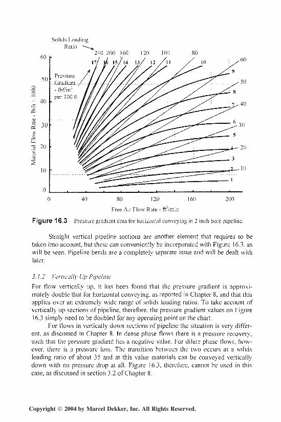
Figure 16.3 is a graph of material flow rate plotted against air flow rate, which isthe usual form for presenting conveying characteristics for materials. In this casethe family of curves that are drawn are lines of constant pressure gradient in Ibf/in2

per 100 ft of pipeline. The data was in i t i a l ly derived from conveying trials withbarite and cement, but has since been found to be reasonably close to that formany other materials. Data in this form has been presented for both horizontal andvertical pipeline runs in earlier sections, notably in Chapters 8 and 15.

3.1.1 Horizontal Pipeline

The data in Figure 16.3 represents the pressure gradient for conveying materialthrough straight horizontal pipeline of 2 inch bore. As will be seen, it covers bothdilute and dense phase conveying, with a smooth transition between the two. ThisQuick Check Method is based on the use of this data and so it w i l l be seen thatthere is no specific reference to material type.

It must be recognized, therefore, that this is also strictly a first approxima-tion method only, but it will provide an entirely different means of obtaining aquick check solution. To the pressure drop for conveying the material must beadded the pressure drop for the air, and this wi l l be considered later. The effect ofpipeline bore must also be considered, and this, of course, is also related to the airflow rate.



Solids LoadingRatio ---.

50

40

oi

o

30

20

10

0

240 200 160 120

\ll \i 15/14 13

100

PressureGradient- lbf/ in2

per 100 ft

20

10

0 40 160 20080 120

Free Air Flow Rate - ft'/min

Figure 16.3 Pressure gradient data for horizontal conveying in 2 ineh bore pipeline.

Straight vertical pipeline sections are another element that requires to betaken into account, but these can conveniently be incorporated with Figure 16.3, aswill be seen. Pipeline bends are a completely separate issue and wi l l be dealt withlater.

3. 1.2 Vertically Up Pipeline

For flow vertically up, it has been found that the pressure gradient is approxi-mately double that for horizontal conveying, as reported in Chapter 8, and that thisapplies over an extremely wide range of solids loading ratios. To take account ofvertically up sections of pipeline, therefore, the pressure gradient values on Figure16.3 simply need to be doubled for any operating point on the chart.

For flows in vertically down sections of pipeline the situation is very differ-ent, as discussed in Chapter 8. In dense phase flows there is a pressure recovery,such that the pressure gradient has a negative value. For dilute phase flows, how-ever, there is a pressure loss. The transition between the two occurs at a solidsloading ratio of about 35 and at this value materials can be conveyed verticallydown with no pressure drop at all. Figure 16.3, therefore, cannot be used in thiscase, as discussed in section 3.2 of Chapter 8.


462 Chapter 16

3.2 Pipeline Bore

Material flow rate varies approximately in proportion to pipe section area, andhence in terms of (diameter)2. Air flow rate, to maintain the same velocity in apipeline of different bore, varies in exactly the same way. To determine the pres-sure gradient for flow in a pipeline having a bore different from that of the refer-ence data in Figure 16.3, both the material and air flow rates should be adjusted inproportion to (d2/2)2, where d2 is the diameter of the plant pipeline in inches. It willbe noted, therefore, that there will be no change in the value of the solids loadingratio.

It must be appreciated that along the length of a pipeline, as the pressuredrops and the conveying air velocity increases, the pressure gradient is likely toincrease. In Figure 16.3 a single value is given for the entire pipeline. This valuecan be taken to be an average for the pipeline, but it is another feature that rein-forces the point that this is only an approximate method.

3.2.1 Stepped Pipelines

When high pressure air is employed it is usual to increase the bore of the pipelineto a larger diameter along the length of the pipeline. This technique was consid-ered in some detail in Chapter 9. By this means the very high velocities that wi l lresult towards the end of a single bore pipeline, from the expansion of the air, canbe prevented.

By this means it is often possible to gain a significant increase in perform-ance of the pipeline. The pressure drop in a stepped pipeline can be evaluated inexactly the same way as outlined above. A critical point in stepped bore pipelinesis the location of the steps along the length of the pipeline. At each step in thepipeline the conveying air velocity must not be allowed to fall below a givenminimum value. The solution, therefore, will be an iterative one since the velocityof the air at the step depends upon the pressure at the step.

3.3 Pipeline Bends

Pressure drop data for bends in pipelines is presented in Figure 16.4. This is anidentical plot to that in Figure 16.3 and covers exactly the same range of convey-ing conditions. The pressure drop in this case is for an individual bend in the pipe-line and hence is in Ibf/in" per bend. The data given in Figure 16.4 relates to 90°radiused bends in a 2 inch bore pipeline. This is also data that was derived fromconveying trials with barite and cement that has since been found to be reasonably-close to that for other materials.

3.3.1 Bend Geometry

As mentioned earlier, it has been found that this pressure drop relationship varieslittle over a range of D/d (bend diameter to pipe bore) ratios from about 5 to 30.



Solids loading

60

50ooo

_0U,

13 20

a

10

ratio60

PressureGradient- tbf/in2

per 100ft

0 40 80 120 160 200

Free Air Flow Rate - ft ' /min

Figure 16.4 Pressure drop data for 90° radius bends in 2 inch bore pipeline.

It has been found that the pressure drop in very sharp or short radius bends,and particularly blind tee bends, however, is significantly higher and so an appro-priate allowance should be made if any such bend has to be used, or is found to befitted into an existing pipeline.

Little data exists for bends other than those having an angle of 90° and so itis suggested that the data in Figure 16.4 is used for all bends, since 90° bends arelikely to be in the majority in any pipeline. In the absence of any reliable data onthe influence of pipeline bore it is suggested that the data in Figure 16.4 is used forall bends, regardless of pipeline bore. For larger bore pipelines the material and airflow rates wil l have to be scaled in the same way as outlined for the straight pipe-line in Figure 16.3.

3.4 Air Only Pressure Drop

As mentioned earlier, the data in Figure 16.3 relates only to the conveying of thematerial through the pipeline, and so the pressure drop required for the air alonemust be added. In Figure 16.5 the influence of pipeline bore on this pressure dropfor 500 ft long pipelines is presented to illustrate the potential influence of thisvariable and is similar to that shown earlier in Figure 6.5.


464 Chapter 16

PipelineBore - 1

Pipe!-500

Conveying Line Exit Air Velocity - ft/min

1000 2000 3000 4000 5000 6000 7000 8000 9000

40 80 120 160

Free Air Flow Rate - ftVmin * (d2/2)2

200

Figure 16.5 Influence of pipel ine bore and air flow rate on the empty pipeline pressuredrop.

Figure 16.5 shows the influence of air flow rate and pipeline bore on con-veying line pressure drop for a representative pipeline length of 500 ft. Since pipebore is on the bottom of Equation 6.3, pressure drop deceases with increase inpipeline bore. Figure 16.5 is presented by way of illustration. The air only pressuredrop for any pipeline can be evaluated as illustrated above in section 2.4.1 and themodels presented in Chapter 6.

It w i l l be seen that conveying line exit air velocity has been added to thehorizontal axis for reference. Conveying line inlet air velocity is the critical designparameter, but this cannot be added conveniently because it is also a function ofthe conveying line inlet air pressure. Because a range of pipeline bores are repre-sented on this plot, the air flow rate is in terms of that for the reference 2 inch borepipeline x (d2/2)2.

From Figure 16.5 it will be seen that the air only pressure drop can be quitesignificant, and particularly so for long, small bore, pipelines. As there are manyvariables in this pressure drop relationship it is probably best to evaluate the pres-sure drop mathematically on an individual basis, using the models presented inChapter 6, as mentioned above

Another graph, plotted for 4 inch bore pipelines, is presented in Figure 16.6to illustrate the influence of pipeline length, with the pressure drop relationshipbeing presented for 100 and 1000 ft long pipelines, as well as the 500 ft long pipe-line of 4 inch bore. This is similar to that shown above in Figure 16.5 and alsoincludes both air flow rate and conveying line exit air velocity on the horizontalaxis.



10

,g

-O

T 6a

I§ 4

PipelineLength - ft

Pipeline Bfrre !- 4 inert

1000

-. 500

100

Conveying Line Exit Air Velocity - ft/min1000 2000 3000 4000 5000 6000 7000 8000 9000

40 80 120 160

Free Air Flow Rate - fVVrnin x (d2/2)2

200

Figure 16.6 Influence of pipeline length and air flow rate on empty pipeline pressuredrop.

3.5 Conveying Parameters

Many of the conveying parameters to be taken into account in the analysis aresimilar to those presented above for the previous method.

5.5.7 Pick-Up Velocity

System design decisions have always to be made with regard to a value of the con-veying line inlet air velocity to be employed. This is critical to the success of anypneumatic conveying system. The data presented in Figure 16.1 and Equations 7to 9 is equally valid here by way of guidance in determining a value for pick-upvelocity. Once again it must be emphasized that if the material is capable of beingconveyed at low velocity in dense phase, then the influence of solids loading ratiowill additionally have to be taken into account.

3.5.2 Influence of Distance and Pressure

The design method presented here is an iterative process, and particularly so fordense phase conveying where the conveying line inlet air velocity is a function ofthe solids loading ratio. Solids loading ratio is an important parameter in this proc-ess, and so the potential influence of conveying distance and air supply pressureon the solids loading ratio is presented in Figures 16.7 and 16.8. These graphswere presented earlier in Figures 4.27 and 4.28 to illustrate the potential capabilityof pneumatic conveying systems.


466 Chapter 16

15

I °tx

-10

150 100 80 60 40

200 300 400Conveying Distance - ft

500

100 80 60 40 30

Figure 16.7 The influence of air supply pressure and conveying distance on solidsloading ratio for low pressure conveying systems.

60

<U

I50

r'c

§ 40

o

30

Q.

% 20C/3

10

ISO 100 80 60

500 1000 1500

Conveying Distance - ft

2000

30

2500

Figure 16.8 The influence of air supply pressure and conveying distance on solidsloading ratio for high pressure conveying systems.



Figure 16.8 is drawn for high pressure, long distance conveying systems,with air supply pressures up to 60 lbf/in2 gauge and pipeline lengths of up to 2500ft. Figure 16.7 is drawn for shorter distance, low pressure systems, up to 15 lbf/in2

500ft.It should be noted that dense phase conveying is possible with low pressure

vacuum conveying systems, as will be seen from Figure 16.7. This is becausedense phase conveying is a function of pressure gradient and does not depend ondistance or pressure drop alone.

Pipeline bore, conveying air velocity, and material type, will all have an in-fluence on the overall relationship and so it must be stressed once again that thesefigures are only approximations for this purpose and on no account should they beused for design purposes alone, as mentioned earlier.

3.6 PROCEDURE

To illustrate the method it is proposed to use the same example as employed in theprevious chapter to demonstrate the procedure with regard to scaling parametersfor dense phase conveying. This was to investigate the conveying potential of thepipeline system illustrated in Figure 15.15 for the conveying of cement. The pipe-line routing included a total of 660 feet of horizontal pipeline, 140 feet of verti-cally up pipeline and eight 90° bends.

It was proposed that a conveying line inlet air pressure of about 30 psigshould be used, with atmospheric pressure at 14-7 psia. It was assumed that thetemperature of the air and cement were 520 R (60°F) throughout. A cement flowrate of 140,000 Ib/h was required and it was considered that an 8 inch bore pipe-line would be required.

The equivalent length of the Figure 15.15 pipeline can be obtained fromEquation 15.9:

Le = Lh + 2 Lv + (N + 2 Leb)

The terms in the equation are as follows:: Lh = total length of horizontal pipeline of 660 ft.i ! Lv= total length of vertically up pipeline of 140 ft._" N = total number of bends, which is eight.

Leh= equivalent length of bends, from Figure 8.18, assuming a convey-ing line inlet air velocity of about 900 ft/min, to be about 10 ft.

Substituting the above set of values into Equation 15.9 gives:

Le = 1040 ft

From Figure 16.8 a typical value of solids loading ratio would be about 40with an air supply pressure of 30 psig and an equivalent length of 1040 ft. FromFigure 13.3 the minimum conveying air velocity for cement conveyed at a solids


468 Chapter 16

loading ratio of 40 is about 700 ft/min and so with a margin of 20% for conveyingline inlet air velocity, the value of 800 ft/min assumed above is satisfactory.

Since a pipeline bore and material flow rate are both specified, it is the ac-tual pressure drop that is required to be evaluated and this comes in three elements.

3.6.1 Straight Pipeline Pressure Drop

This can be obtained from Figure 16.3. This is drawn for a 2 inch bore pipelineand so the material flow rate needs to be scaled down by using Equation 15.12:

d,

= 140,000

= 8750 Ib/h

To use Figure 16.3 any two reference points are required and it will be seenthat for a material flow rate of 8750 Ib/h and a solids loading ratio of 40, the pres-sure gradient is approximately 4 Ibf/in2 per 100 ft of pipeline and the free air flowrate is about 55 ft'/min.

The pressure drop due to the material, therefore, is s imply given by the pres-sure gradient multiplied by the equivalent length:

x [660 + (2 x 140100

= 37-6 Ibf/in2

3.6.2 Pipeline Bends

From exactly the same location on Figure 16.4 the pressure drop due to the bendsis given as 0-6 Ibf/in2 per bend and so the total for the bends is:

Apb = 8 x 0 - 6= 4-8 Ibf/in2

3.6.3 Air Only

From Equation 6.10 the pressure drop due to the air is given by:

f L £ k p C2

21,600 d 1,03 6,800



The terms in the equation are as follows:/ = 0-004. This is the pipeline friction coefficient. This is derived from

Figure 6.3, having evaluated the Reynolds number for the flow (see Chap-ter 6 section 2.1.4) in the usual way.

1 L = 800 ft. This is the actual length of the pipeline in this case.; ! d = 8 inch. This i s the diameter of the pipeline.. ZA= This is the loss coefficient for all the bends in the pipeline. For anindividual bend the value of k is about 0-15 (see Figure 6.6).

i p = 0-0765 Ib/fV. This is the approximate density of the air at the end ofthe pipeline.

i C = 3000 ft/min. This is the approximate velocity at the end of the pipe-line. This is only an estimate at this stage and may have to be re-considered if an iteration is required at the end of the calculation process.

gc = 32-2 ft Ib/lbf s2. This is the gravitational constant.

Substituting values gives:

0 - 0 0 4 x 8 0 0 8 x 0 - 1 5 ^ 1 0 • 0765 x 30002

121,600x8 1,036,800,1 3 2 - 2

= 0-42 lbf/in2

3.6.4 Total System

The total pressure drop for the pipeline, Apc, is the sum of the three elements:

Apc = App + Apt, + Apa

= 37-6 + 4-8 + 0-4= 42-8 lbf/in2

A check now needs to be made on the values obtained to ensure that they are

consistent. The free air flow rate, VQ , was 55 mVmin in the two inch bore pipe-

line. This equates to 880 ft /min in an eight inch bore pipeline. From Equation5.11:

C = 5-19 -^2- ft/min


i . 71/ = conveying line inlet air temperature of 520 R.

T i V0 = volumetric flow rate of free air of 880 m3/min.

i d = pipeline bore of 8 in._! pi = conveying line inlet air pressure of 44-0 + 14-7 lbf/in2 abs


470 Chapter 16

Substituting these values gives:

C, = 632 ft/mm

A check also need to be made on the value of solids loading ratio. For thiscalculation a value of air mass flow rate is required. This can be obtained quitesimply by multiplying the value of free air flow rate by the value of free air den-sity. Thus the solids loading ratio, $ is:

mp _ 140,000

p VH 0 • 0765 x 880 x 60

= 35

It will be seen from this check that both the solids loading ratio and the con-veying line inlet air velocity (and hence free air flow rate) are slightly below theinput values and so it would be recommended that the procedure be repeated onthe basis of the new data. Alternatively a higher air supply pressure could be usedor a larger bore of pipeline. However, since the first estimate is very close, it isalmost certain that with a stepped pipeline the conveying duty would be achievedsatisfactorily. There are many alternatives and possibilities.

Since a wide range of pipeline bore and air supply pressure combinationswill be capable of achieving the duty, it is always worthwhile investigating a num-ber of different options, as they are likely to lead to different system costs andoperating power requirements.

4 STEADY FLOW ENERGY EQUATION METHOD

The steady flow energy equation, in its fu l l form, includes a heat transfer term, aswell as a work transfer term and includes changes of both kinetic energy and po-tential energy, as well as changes in enthalpy. In this application heat transfer be-tween the system and the surroundings can be disregarded and so the only energyinput to the system that needs to be taken into account is that imparted by the airmover. The appropriate thermodynamic model is presented in detail below.

The energy input to the system from the air mover is transferred to both theconveyed material, and the conveying air, and so both must be included. It is con-sidered that changes in enthalpy can also be disregarded, but changes in both ki-netic and potential energy are included in the energy terms, and these are also pre-sented in detail below.

4.1 The Model

In this model the thermodynamic work imparted to the air by the compressor, orexhauster, Wa, is equated to the energies transferred to the conveyed material, Ep,



and to the conveying air, Ea. Energies in this model are expressed in terms of a'head', h, or equivalent potential energy. Thus:

Wa = Ep + Ea hp - - - - - - - - - (23)

4.1.1 Applicability

The influence of conveying air velocity, pipeline bore, horizontal conveying, ver-tical lift, pipeline bends and plant elevation are all taken into account. The modelcan be applied equally to vacuum conveying and to positive pressure conveyingsystems. It will also apply to both dilute and dense phase conveying, provided thatthe conveying parameters are correctly specified. Although the model can theo-retically be applied universally it must be stressed once again that there is no refer-ence to material properties anywhere in the basic equations.

As with the previous methods considered, it is also possible to apply con-stants to the models presented, at appropriate points in the equations. These con-stants can be used to fine tune the model, for a given material, so that the modelcan be applied with a reasonable degree of reliability for the design of pipelinesystems for that specific material. Ideally, actual conveying data for the given ma-terial should be used for this purpose. By this means different sets of constants canbe determined to cater for a range of different materials, or for a number of differ-ent grades of a particular material.

4.2 COMPONENTS OF MODEL

The three basic terms of the model, presented in Equation 16.23 are detailed be-low. The energy input is just a single term as this relates to the work done by thecompressor or exhauster. The energy transfer to both the conveyed material andthe air are split into their component parts and it is with these than fine tuning canbe applied with the use of constants to improve the accuracy of the overall modelfor a given material.

4.2.1 Energy Input to Conveying Pipeline

The compression or expansion of the air, particularly within positive displacementmachines, is an adiabatic process and the useful work imparted to the air, Wa, isgiven by:

m \p v - p vw a v 4 4 3 3 • .Wa = -; r hp - - - - - (24)

229•2(n - l)

where ma = mass flow rate of conveying air - Ib/min

(see Equation 25)p = air pressure - lbf/in2 abs


472 Chapter 16

v = specific volume of air - f t ' / lb(see Equation 27)

and n = adiabatic index for compression of air- 1-2

subscript 3 relates to the inlet conditions to the air moverand 4 relates to the exit conditions from the air mover

(see Figures 16.9 and 16.10at the end of this chapter)

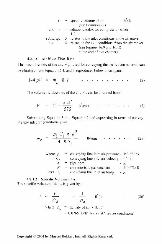
4.2.1.1 Air Mass Flow Rate

The mass flow rate of the air, ma , used for conveying the particulate material can

be obtained from Equation 5.4, and is reproduced below once again:

\44pV = m R T - - - - - - - - - - ( 2 )

The volumetric flow rate of the air, V , can be obtained from:

n d2

V = C * fr'/mjn . . . . . . . (3)576

Substituting Equation 3 into Equation 2 and expressing in terms of convey-ing line inlet air conditions gives:

2P-, C, n d

mn = — Ib/min - - - - - - (25)a 4 R T,

where p/ = conveying line inlet air pressure - lbf/in2 absCt = conveying line inlet air velocity - ft/mind = pipe bore - mR = characteristic gas constant - ft lbf//lb R

and TI = conveying line inlet air temp - R

4.2.1.2 Specific Volume of AirThe specific volume of air, v, is given by:

V 1ft'/lb - - - - - (26)

ma Pawhere pa = density of air - lb/ft3

= 0-0765 Ib/ff for air at 'free air conditions'



and from the Ideal Gas Law (Equation 2)

R Tftj/lb (27)

so that

144 p

R T^

144 p,etc

4.2.1.3 Adiabatic CompressionFor adiabatic processes we have the following basic relationship between/; and v.

P\v\ =

Note also that:

P\v\ _

'1Ti "i

(29)

andT1">

V2 (30)

4.2.2 Energy Transfer to Conveyed Material

As mentioned above, energies are expressed in terms of a head. For the conveyedmaterial, therefore, the vertical l i f t in the pipeline is taken as the reference, ratherthan the length of horizontal pipeline, as is generally common with most otherpneumatic conveying system design methods.

The energy transfer to the conveyed material, Ep, is given by:

m g hP P hp

where trip = flow rate of conveyed material - Ib/h

g = gravitational acceleration = 32-2 ft/s2

(31)


474 Chapter 16

gt. = gravitational constant = 32-2 ft Ib/Ibf s2

and hp = total system head loss forconveyed material - ft

4.2.2.1 System Head LossThe total system head loss for the conveyed material, hp, is the sum of the compo-nent parts of the energy required to accelerate the particles to their terminal veloc-ity, hk, and to convey the material through the horizontal, h/,, and vertical, /!,,, sec-tions of the pipeline, and the bends, Nhb. Thus:

hp = hk + hh + hv + Nhb ft - - - - - (32)

where h/, = average head loss per bend due to particlesand N = total number of bends in pipeline

4.2.2.1.1 Acceleration Loss

0-8 C2]hk = J— f t - - - - - - - - (33)

7200 g

where C? = conveying line exit air velocity - ft/minand g = gravitational acceleration - ft/s2

Note:The constant (0-8) accounts for the fact that the particles will typically be

conveyed to a terminal velocity which is about 80% of that of the convey-ing line exit air velocity, C3 (see Figure 15.10).

4.2.2.1.2 Horizontal Line Loss

hh = lhLh ft - - (34)

where L/, = total length of horizontal pipeline - ftand /I/, = horizontal line constant - -

Note:The constant, 1;, accounts for the fact that the head loss is in terms of an

equivalent length of vertically upward pipeline.1 The value of this constant is clearly influenced by friction forces between

particles, and particles and pipe walls, and is likely to be affected quitesignificantly by material type. It is suggested that a value of 0-5 should beused in the first instance:



4.2.2.1.3 Vertical Line Loss

hv = 1VLV ft (35)

where L,, = total length of vertically upsections of pipeline - ft

and A,, = vertical line constant - -

Note:The value of the constant A,, is also clearly influenced by friction forces

between particles, and particles and pipe walls, and is likely to be affectedquite significantly by material type. It is suggested that a value of 1 -0should be used in the first instance:

[J Vertically downward sections of pipeline can be disregarded, providedthat no individual section is longer than about 15 ft. For longer sections ofconveying vertically down refer to Chapter 8.

4.2.2.1.4 Bend LossesAverage bend loss:

hh = A,C'

7200 g(36)

where C = root mean air velocity

f ? -sO-5Cl+Cl

2

- ft/min

ft/min (37)

C/ = conveying line inlet air velocity - ft/minC2 = conveying line exit air velocity - ft/ming = gravitational acceleration - 32-2 ft/s2

and X\, = pipeline bend constant - -

Note:j The value of the constant ).h will be influenced by both the type of con-veyed material and the bend geometry. It is suggested that a value of 1 -5should be used in the first instance:

'..• The velocity of the air increases through the pipeline from C/ to C2 andso the head loss for every bend will be different. The root mean velocity istaken in order to provide an average value for the head loss. In general thebends are distributed uniformly along the length of the pipeline. Only ifthere is an unbalanced cluster of bends at the end of pipeline wil l this bendloss need to be reconsidered.


476 Chapter 16

4.2.2.2 Total Energy TransferIf the individual elements of head loss are substituted back into Equation 16.32and this, in turn, is substituted into Equation 16.31, the result gives the total energytransfer to the conveyed material.

m 8

x l O 7200g

NC2

7200ghp (38)

4.2.3 Energy Transfer to Conveying A ir

The energy transfer to the conveying air, £„, needs to be considered in terms offriction losses. These are pipe wall friction and bend losses. This is given by:

m g ha a

33,000 ghp (39)

where ma = air mass flow rate - Ib/min

g = gravitational acceleration = 32-2 ft/s"hu = total system head loss for

conveying air - ftand gc = gravitational constant =32-2 ftlb/lbfs2

4.2.3.1 System Head LossThe total system head loss, /?„, is the sum of that due to the pipeline wall friction,h/, and pipeline bends, Nhha. Thus:

+ Nh.'ba ft

where hf = pipeline friction head loss - ftN = number of bends - -

and hf,a = head loss per bend due to air - ft

(40)

4.2.3.1.1 Pipeline Friction Loss

48 / L C2

xd

(41)

where / = pipeline friction coefficient



L

dg

and C

4.2.3.1.2 Bend Loss

d khba =

where dk

f

= 0-0045 typically for p ipel ine~ total pipeline length= Lh + £,.= pipeline bore= gravitational acceleration

= root mean air velocity(see Equation 37)

- ft

- in- 32-2 ft/s2

- ft/min

(42)

- inpipeline borebend head loss coefficient0-15 typically for radiused bendspipeline friction coefficient0-0045 typically

Substituting values for k and/, the total head loss due to the bends wil l be:

Nh baN d

1-44(43)

4.2.3.2 Total Energy TransferIf the individual elements of head loss are substituted back into Equation 41 andthis, in turn, is substituted into Equation 39, the result gives the total energy trans-fer to the conveying air.

hp - - (44)ma g

c

/(V^v)c2

150 g d

N d

1-44

4.3 Procedure

The energy equation model presented in Equation 23 and the three components ofthe equation have been presented in detail above. It is possible to equate the workterm in Equation 24 to the energy terms for the conveyed material and the convey-ing air in Equations 38 and 44 in a single line and solve. This is not included hereas a further numbered equation since it is felt that a better understanding of theprocess will be gained by evaluating the constituent parts individually.


478 Chapter 16

To illustrate the method it is proposed to use the same example as employedearlier in this chapter to illustrate the universal conveying characteristics methodwhich, in turn, was used to demonstrate the procedure with regard to scaling pa-rameters in the previous chapter. By this means the results of all three methods canbe compared, and in particular, these two quick check methods with each other,and with the more reliable method of using scaling parameters based on the use ofactual conveying data.

To recap, a sketch of the pipeline is given in Figure 15.15 and the routingincludes a total of 660 ft of horizontal pipeline, 140 ft of vertically up pipeline andeight 90° bends. It was proposed that a conveying line inlet air pressure of about30 psig (pi = 44-7 psia) should be used, with atmospheric pressure, p2, at 14-7 psia.A cement flow rate of 140,000 Ib/h was required and it was considered that an 8inch bore pipeline would be required.

For the convenience of calculation it was assumed that the temperature ofthe air and cement were 520 R (60°F) throughout, but for this particular method itmust be emphasized that the temperature of the air leaving the compressor must becalculated, since it will be at a very much higher temperature and the value of thespecific volume of the air at this point is a function of this temperature (see Equa-tion 27).

Once again it will have to be an iterative process, since the material is capa-ble of being conveyed in dense phase, and so a conveying line inlet air velocitywill have to be selected in order to allow the calculation to proceed. In terms of asolution it is proposed that the material flow rate achieved in an 8 inch bore pipe-line and with a conveying line inlet air pressure of 30 psig should be investigated.Any one of the three parameters can be chosen but this is probably the easiest interms of solving. Results can be obtained relatively quickly and so a wide range ofconveying parameters can be conveniently investigated.

4.3.1 Compressor Work

The expression for compressor work is given in Equation 24. This requires a valuefor air mass flow rate and so a conveying line inlet air velocity must be specified.This wi l l have to be an estimate to allow the calculation process to proceed, and soa value of 720 ft/min (20% margin on minimum value) is taken in anticipation ofthe solids loading ratio being greater than about 40 (see Figure 15.16). Air massflow rate is given by:

n d1 p Cm = Ib/min - - - - - - - - 6.15

4 R T

Substituting conveying line inlet air values presented above gives an airmass flow rate of 58-4 Ib/min. Specific volume values are also required in Equa-tion 24 and these can be evaluated using Equation 27. 7j, the temperature at inlet



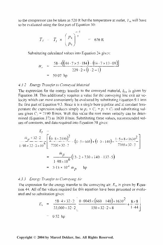
to the compressor can be taken as 520 R but the temperature at outlet, T4, wil l haveto be evaluated using the first part of Equation 30:

T4 = T; = 626 R

Substituting calculated values into Equation 24 gives:

5 8 - 4 [ ( 4 4 - 7 x 5 - 1 8 4 ) - ( l 4 - 7 x l 3 - 0 9 ) ]

2 2 9 - 2 x ( l . 2 - l )

= 50-07 hp

4.3.2 Energy Transfer to Conveyed Material

The expression for the energy transfer to the conveyed material, Ep, is given byEquation 38. This additionally requires a value for the conveying line exit air ve-locity which can most conveniently be evaluated by substituting Equation 9.1 intothe first part of Equation 9.3. Since it is a single bore pipeline and at constant tem-perature the expression reduces simply to pt x C, = p2

x C? and substituting val-ues gives C? = 2190 ft/min. With this value the root mean velocity can be deter-mined (Equation 37) as 1630 ft/min. Substituting these values, recommended val-ues of constants, and data required into Equation 38 gives:

mp x 3 2 - 2

l - 9 8 x 3 2 - 2 x ! 0 6

( 0 - 8 x 2 1 9 0 )

7 2 0 0 x 3 2 - 2,((, 5x66o )n-0 A v 1 Af)\ _i_

• 5 x 8 x l 6 3 0 2

7 2 0 0 x 3 2 - 2

m ,

1 - 9 8 x 1 0

= 3-13 x 10'4 m

-(13-2 + 330 + 140 + 137-5)

p

4. 3. 3 Energy Transfer to Conveying A ir

The expression for the energy transfer to the conveying air, Ea, is given by Equa-tion 44. All of the values required for this equation have been presented or evalu-ated and so substitution gives:

Ea =5 8 - 4 x 3 2 - 2

33 ,000x32-2

= 0-52 hp

1 5 0 x 3 2 - 2 x ! 1 - 4 4


480 Chapter 16

4.3.4 Material Flow Rate

By substituting these component parts into the basic model, Equation 23, gives:

50-07 = 3-13 x 10"4 mp + 0-52

and mp = 158,300 Ib/h

Based on this value of material flow rate the solids loading ratio, for the airflow of 58-4 lb/min, comes to about 45. As a consequence the value of conveyingline inlet air velocity chosen is satisfactory and so the calculation is complete withno iteration required. The flow rate of cement obtained at 158,300 Ib/h is about13% greater than that derived by using the scaling parameters presented in theprevious chapter. If actual conveying data is available it would be recommendedthat the various constants incorporated into the equation should be 'fine tuned' inorder to increase the reliability of the method.

NOMENCLATURE

Symbol SI

A Pipe section area in~ m7

n d= for a circular pipe

4C Conveying air velocity ft/min m/s

C Root mean velocity ft/min m/s

2 2C, +C2

d Pipeline bore in mE Energy transfer hp kW/ Pipeline friction coefficientg Gravitational acceleration ft/s2 m/s2

32-2 9-81gL. Gravitational constant ft Ib/lbf s" kg m/kN s2

32-2 1-0h Head loss or gain ft mk Bend loss coefficientL Pipeline length ft m

ma Air mass flow rate lb/min kg/s



m p Material flow rate

n Adiabatic indexA' Number of bendsp Air pressureP Power requiredR Characteristic gas constant

= for airl TemperatureT Absolute temperature

v Specific volume of air

V Volumetric flow rate of airW Work done

Greek

Air density= at free air conditions

Solids loading ratio

mp

Ib/h

lbf/in2 abshpft Ibf/lb R53-3op

Rt°F + 460ft3/lb

ftYminhp

Ib/ft'0-0765

m

X Conveying parameter constanti// Total pipeline head loss coefficient

Superscripts

n Adiabatic index

Subscripts

a Conveying airatm Atmospheric valueb Bendsc Material conveyinge Equivalent valuef Frictionh Horizontalk Acceleration or kinetic valuemin Minimum valuep Conveyed material or particlesv Vertically up

tonne/h

kN/nr abskWkJ/kg K0-287°CK.t°C + 273m3/kg

nrYskW

kg/m3

I-225

o Free air conditions


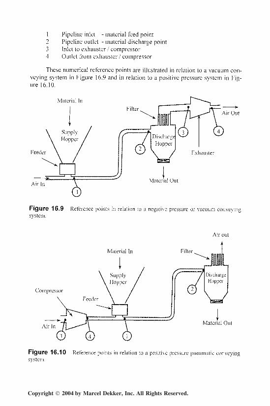
482 Chapter 16

Pipeline inlet - material feed pointPipeline outlet - material discharge pointInlet to exhauster / compressorOutlet from exhauster / compressor

These numerical reference points are illustrated in relation to a vacuum con-veying system in Figure 16.9 and in relation to a positive pressure system in Fig-ure 16.10.

Material In

Feeder

Air In Material Out

Figure 16.9 Reference points in relation to a negative pressure or vacuum conveyingsystem.

Compressor

Air In

Material In

Air out

Filter,

Material Out

Figure 16.10 Reference points in relation to a positive pressure pneumatic conveyingsystem.



Note:;~ In a negative pressure system; pt will be slightly below atmospheric pres-

sure if an artificial resistance is added to the air pipeline inlet for the pur-pose of assisting the feed of material into the pipeline;/}? and Tj will gen-erally be equal to p3 and T3; but the mass flow rate of air at 3 might behigher than that at 2 if there is a leakage of air across the material outletvalve on the discharge hopper.

In a positive pressure system; p, wil l generally be equal \.op4 unless thereis a pressure drop across the feeding device; p2 and p3 will generally beequal to the local atmospheric pressure; and the mass flow rate of air at 1wil l be lower than that at 4 if there is a leakage of air across the feedingdevice.

Prefixes

A Difference in value1. Sum total

REFERENCE

1. D. Mills. A quick check method for the design of pneumatic conveying systems. Proc26th Powder & Bulk Solids Conf. pp 107-124. Chicago. May 2001.Subsequently published in Advances in Dry Processing. Cahners, pp 7-17. Nov 2001.


Handbook of Pneumatic Conveying Engineeringnguyen.hong.hai.free.fr/EBOOKS/SCIENCE AND... · 448...

Documents

Transcript of Handbook of Pneumatic Conveying Engineeringnguyen.hong.hai.free.fr/EBOOKS/SCIENCE AND... · 448...