Handbook for Agrohydrology (NRI) - Your.org
223
Home "" """"> ar .cn .de .en .es .fr .id .it .ph .po .ru .sw Handbook for Agrohydrology (NRI) Chapter 3: Erosion and sedimentation data (introduction...) 3.1 Soil erosion 3.2 Field measurement of sediments (eroded material) 3.3 Laboratory analysis Equipment costs Appendix B: Erosion and sedimentation data Handbook for Agrohydrology (NRI) Chapter 3: Erosion and sedimentation data This chapter covers five main topics: - The estimation of soil loss by the application of empirically derived equations. - Methods of measuring soil loss by the collection of the total amount of eroded material from runoff/soil erosion plots. - Methods of sampling runoff that are carried in suspension to determine overall soil losses. 21/10/2011 Handbook for Agrohydrology (NRI) D:/cd3wddvd/NoExe/Master/dvd001/…/meister11.htm 1/223
Transcript of Handbook for Agrohydrology (NRI) - Your.org

Home"" """"> ar.cn.de.en.es.fr.id.it.ph.po.ru.sw
Handbook for Agrohydrology (NRI)
Chapter 3: Erosion and sedimentation data
(introduction...)
3.1 Soil erosion
3.2 Field measurement of sediments (eroded material)
3.3 Laboratory analysis
Equipment costs
Appendix B: Erosion and sedimentation data
Handbook for Agrohydrology (NRI)
Chapter 3: Erosion and sedimentation data
This chapter covers five main topics:
- The estimation of soil loss by the application of empirically derived
equations.
- Methods of measuring soil loss by the collection of the total amount of
eroded material from runoff/soil erosion plots.
- Methods of sampling runoff that are carried in suspension to determine
overall soil losses.
21/10/2011 Handbook for Agrohydrology (NRI)
D:/cd3wddvd/NoExe/Master/dvd001/…/meister11.htm 1/223
- Methods of laboratory analysis that determine the quantities of
suspended soil material.
- Methods of laboratory analysis that determine soil particle size.
For practical purposes, soil erosion is regarded as the detachment of soil materials
from their previous location. Sedimentation is the transport and deposition of
eroded soil and although erosion due to wind occurs, the main transporting agent
in almost all environments is water. Thus the theoretical calculation of soil losses
are covered by estimates of erosion, whereas the actual measurement of material
lost from a catchment is regarded as the measurement of sedimentation.
The erosion that leads to a wide range of environmental problems is usually the
result of human activity; such as deforestation, cultivation and over-grazing, and
is intimately linked with the runoff process. Agriculture is often a powerfu1 agent
in promoting soil erosion and water harvesting frequently exploits the conditions
that promote runoff and which can intensify rates of soil removal. The processes
of sedimentation are frequently attendant.
Soil loss data are expressed in terms of weight per unit area, for example tonnes
per hectare, per season. The measurement of sedimentation, the quantification of
eroded soil materials, is likely to be of importance to projects that engage in the
activities of agrohydrology and methods of reducing soil erosion are an important
aspect of this book. A background is given to the main methods of erosion control,
below, but the mechanical and constructional aspects of these controls are
discussed in detail in chapter 7, Water Harvesting.
21/10/2011 Handbook for Agrohydrology (NRI)
D:/cd3wddvd/NoExe/Master/dvd001/…/meister11.htm 2/223
3.1 Soil erosion
The climatic factors that influence erosion and sedimentation processes are chiefly
rainfall amount and intensity, which largely determine rainfall energy and runoff
quantity, though the relation between them and soil loss is very complex..
Vegetation cover reduces rainfall energy and retards surface water flow,
encourages infiltration through the physical perforation of soils and the reduction
of the soil moisture reserve. Topography determines land slope and the length of
flow of surface runoff, while the character of soils themselves, in terms of texture,
structure, density, etc., influences the rate at which soil loss and sedimentation
will take place.
Erosion can be summarised as taking five characteristic forms:
Rain splash erosion is the local movement of soil particles under the influence of
raindrop impact. Soil particles are detached from the soil surface, elevated by the
action of splash and return to the surface somewhat lower down the land slope.
Areas with high slopes suffer from such erosion to a much greater extent than flat
land. Large quantities of soil are removed from their original ground location by
the action of raindrops. The energy equation that relates rainfall energy to
intensity, developed by Wischmeier and Smith is of the form:
(kinetic) Energy, E 12.1+8.9 i where (3.1)
E is in m-Mg/ha-mm (metre-metric tonnes per hectare-millimetre) and rainfall
intensity "i" is in mm h-1
21/10/2011 Handbook for Agrohydrology (NRI)
D:/cd3wddvd/NoExe/Master/dvd001/…/meister11.htm 3/223
Clearly such factors as wind direction, drop size, velocity and the nature of the soil
will also affect the quantity of erosion that occurs and although small, clayey
particles are more easily transported than larger sandy ones, they are not so
easily detached from the soil surface.
Sheet erosion is a simplified term for the formation of extremely small channels or
rills. These are created under the influence of rain splash and microscopic
topographical variability and their wandering causes the eventual erosion of soil in
the manner of a sheet. For a given soil and vegetation cover, the erosive power of
the overland flow will be related to its velocity and depth.
When runoff concentrates into small streamlets Rill erosion takes place, forming
small channels. These channels are clearly visible, but their size is such that they
can be obliterated by ploughing. The concentration of flow into rills is particularly
important because it leads to the concentration of runoff, increasing its velocity
and erosive power. On high slopes and shallow soils such erosion can be
destructive.
Gully erosion occurs when channel flow is sufficient to overcome tillage practices
and is yet another stage of the increasing concentration of runoff, even though it
may take place on an ephemeral basis. Gullies extend by the cutting back of their
head and by progressive channel erosion, but stabilisation may occur naturally as
the channel becomes harmonious with its slope and vegetation growth is
established
Stream channel erosion is dissimilar to gully erosion in that it represents a
process that occurs in channels with lower gradients, in which streams often flow
21/10/2011 Handbook for Agrohydrology (NRI)
D:/cd3wddvd/NoExe/Master/dvd001/…/meister11.htm 4/223

continuously. Suspended material is carried along without contact with the bed,
while material moved by the process of saltation bounces or skips along. The bed
load is rolled or pushed along the channel bottom.
Soil erosion is a natural recycling process that has continued throughout
geological time and has been responsible for the formation of sedimentary
deposits that are now the major components of the continental land masses and
sea floor. Tolerable rates of erosion have been suggested as being between 5 and
10 tonnes per hectare per year, but extremely different local circumstances of soil
depth, formation and productivity make such values rather meaningless.
Influences on Sedimentation
Catchment Size. Generally, an increase in catchment size reduces the proportion of
material removed (the "sediment delivery ratio"). This is due the increased
opportunities for the entrapment of sediment within the catchment area. The
presence of flood plain areas adjacent to large streams and rivers provides an
environment for deposition that does not exist with smaller, steeper channels.
Topography and Channel Density. Important topographic factors that influence
sediment removal are channel slope and the channel density of a catchment. The
sediment delivery ratio is highest for steep channels with well defined courses,
rather than low slope streams with ill defined channels. The use of channel density
factors (see chapter 6) is common in the regression analysis of sedimentation
data.
Precipitation and Runoff Regimes are critical factors in determining the removal of
21/10/2011 Handbook for Agrohydrology (NRI)
D:/cd3wddvd/NoExe/Master/dvd001/…/meister11.htm 5/223

sedimentary material. Streams of a flashy nature are effective at its removal. High
intensity storms not only give large runoff amounts, but also increase soil erosion
by rain splash from high energy drops. Catchments that suffer from such storms
display high delivery ratios.
Loss of Vegetation Cover and Agricultural Activity play a major part in creasing
soil erosion.
These influences are built in to the theoretical models of soil erosion that are
discussed below.
3.1.1 Theoretical Estimates of Soil Erosion
a. Universal Soil Loss Equation (USLE)
The Universal Soil Loss Equation (USLE) is widely known and was developed in
many locations of the US by Wischmeier and Smith. In the 1978 publication (USDA
Handbook 537), site data from US locations are given. For example, the full set of
data of which Table 3.3 is a sample, covers 160 crop to fallow conversion ratios of
soil loss (see Appendix B). The USLE is used to determine the value of
conservation measures in farm planning and predicts non-point sediment losses.
As its name suggests, it is the most widely accepted method of estimating soil
loss and has generated variations that are adapted to various local conditions.
Special note is made of the difficulty of applying sod-based rotations in semi-arid
areas as are soil and moisture conservation opportunities of residue/mulch
management (Table 3.3). However, it is important to point out that despite the
simplification of the variables involved in the erosion process by the USLE, its use
21/10/2011 Handbook for Agrohydrology (NRI)
D:/cd3wddvd/NoExe/Master/dvd001/…/meister11.htm 6/223

is often limited because the evaluation of these variables has not been achieved in
many regions of the world. Those wishing to apply the USLE are recommended to
obtain Handbook 537, but an outline of procedures is presented below. The
average annual soil loss is given by:
A = 2.24 RKLSCP where (3.2)
A = average annual loss of soil in Mg ha-1 (tonnes ha-1)
R = rainfall and runoff erosivity index by geographical location
K = soil erodibility factor
LS = topographic factor
C = crop management factor
P = conservation practice factor
The factor R was found (under fallow conditions) to be related to the maximum 30
minute rainfall intensity and the kinetic energy of storms. The factor K in t ha-1
was assessed by measurements of actual soil loss for a series of soils with a range
of physical and chemical properties. The factor LS converts soil losses from the
experimental plot length and slope (22m and 9%, respectively). The conversion
formulae for different slopes and values of L are:
L =(1/22)x and (3.3)
S=(0.43 + 0.30s + 0.043s2)/ 6.574 where (3.4)
x - a constant, 0.5 for slopes > 4%, 0.4 for slopes 4% and 0.3 for slopes < 3%
I = slope length in m
21/10/2011 Handbook for Agrohydrology (NRI)
D:/cd3wddvd/NoExe/Master/dvd001/…/meister11.htm 7/223

s = field slope in %.
C, the cropping management factor includes the effects of cover, crop sequence,
length of season, tillage and storm time distribution. Conversions may be made
from cropping to continuous fallow. P, the conservation practice value,
discriminates between contouring, strips and terraces. Terraces alter the value of
the slope length L, which becomes the terrace interval for losses from the terrace,
whereas if losses from the terrace channel are required, the contour factor is
applied.
Table 3.1: Values of R for Different Return Periods, Annual and Single Storms, USA
Estimates of soil losses can be made and if found to be unacceptable, the
manipulation of farm management and conservation practices can be planned for
its reduction: for example contour and terrace size and intervals. Although soil
loss in terms of t ha-1 (with account taken of economic productivity) is the usual
criterion by which the acceptability of erosion is judged, the effects of
sedimentation may demand that smaller soil losses should be aimed for.
21/10/2011 Handbook for Agrohydrology (NRI)
D:/cd3wddvd/NoExe/Master/dvd001/…/meister11.htm 8/223

Tables 3.1 to 3.3 and Figure 3.1 give typical values for the variables in equation
3.1.
Table 3.2: Soil Erodibility Factor, K, by Soil Texture in Mg ha-1 (t ha-1) *
21/10/2011 Handbook for Agrohydrology (NRI)
D:/cd3wddvd/NoExe/Master/dvd001/…/meister11.htm 9/223

Table 3.3: Ratio of Soil Losses from Crops to Corresponding Loss from Continuous
Fallow
Crop stages:
0 Turnploughing to seabed preparation: 1 Seedbed to first month after seeding: 2
Establishment to second month: 3 Growing cover from 2 months: 4 stubble or
residue to new seedbed.
21/10/2011 Handbook for Agrohydrology (NRI)
D:/cd3wddvd/NoExe/Master/dvd001/…/meister11.htm 10/223
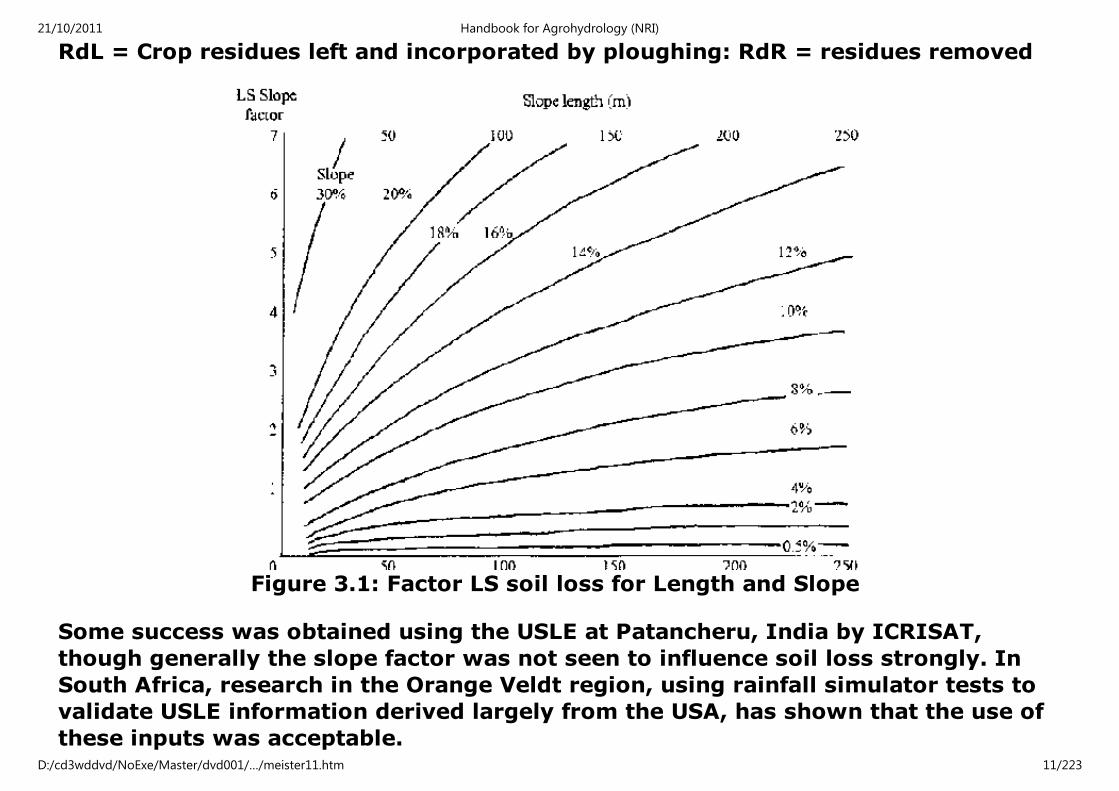
RdL = Crop residues left and incorporated by ploughing: RdR = residues removed
Figure 3.1: Factor LS soil loss for Length and Slope
Some success was obtained using the USLE at Patancheru, India by ICRISAT,
though generally the slope factor was not seen to influence soil loss strongly. In
South Africa, research in the Orange Veldt region, using rainfall simulator tests to
validate USLE information derived largely from the USA, has shown that the use of
these inputs was acceptable.
21/10/2011 Handbook for Agrohydrology (NRI)
D:/cd3wddvd/NoExe/Master/dvd001/…/meister11.htm 11/223

Table 3.4 below gives values for recommended conservation practices. These are
greatly simplified from the complex indices given by Wischmeier and Smith (1978)
which include values for rangeland, pasture, crops, woodland mulches, etc. Slope
length limits are derived from work by the US SCS.
Table 3.4: Recommended Conservation Practices
Worked Example
Calculate the annual soil loss for a location with R= 310, loamy sand soil with K=
0.10 (Table 3.2), C = 0.32 (Table 3.3) length L= 60 m and slope S =12%.
From Figure 3.1, LS=2.5 and the field is to be contoured, therefore from Table 3.4,
PC=0.5.
Annualsoilloss = 2.24 × 310 ×x 0.1 × 2.5 × 0.32 × 0.6 = 33.3 Mg ha-1
A reduction of these levels of soil loss would appear desirable. This must be
undertaken by changing the cropping factor C and/or the conservation practice P
and thereby reducing the value of these indices.
21/10/2011 Handbook for Agrohydrology (NRI)
D:/cd3wddvd/NoExe/Master/dvd001/…/meister11.htm 12/223

b. Modified USLE
The replacement in the USLE, of the rainfall energy factor with a runoff energy
factor, has been undertaken in the USA. The equation of prediction is:
Y = 11.8 (Qqp) 0.56 KCPSL (3.5)
All components of the equation are as for USLE, except the energy factor, 11.8
(Qqp) 0.56 where Q = runoff volume in m³ and qp is the peak flow in m³ s-1.
A combination of measurements from a variety of catchments were tested against
this equation and the results encouraging, however the limitations in this model
must be regarded as being similar to the original USLE model.
c. Soil Loss Estimation for Model for Southern Africa (SLEMSA)
This model was developed in Zimbabwe, following disappointing results using the
USLE. It is based on defined agroecological zones, their physical environments and
soils. In particular, the concentration of the USLE on cropped areas and cropping
systems was regarded as unsuitable in a region where rangeland conditions are
very important. The structure of the model is shown in Figure 3.2 which also
provides details of the model components. However, values of many of these
components have not yet been determined outside Zimbabwe. Some extrapolation
of the model to other countries in the region has been made, but this work has
largely depended upon the direct translocation of experimentally-derived values
from Zimbabwe, in particular the regression coefficients for the bare soil sub
model K, and the soil erodibility factor F. Other components can be measured or
21/10/2011 Handbook for Agrohydrology (NRI)
D:/cd3wddvd/NoExe/Master/dvd001/…/meister11.htm 13/223

determined at a location. Compared to USLE, this model may become more widely
used because of the relative simplicity in obtaining empirical values.
Figure 3.2: Structure and Components of the SLEMSA Model
Empirical studies have defined the values of the parameters K, C, and X in the
following terms.
E = Seasonal rainfall
energy
Joules
m²
Energy of mean annual rainfall
F = Soil erodibility - Index of soil characteristics related to known
erodibilities
i - Rainfall energy
intercepted
% Vegetation cover
21/10/2011 Handbook for Agrohydrology (NRI)
D:/cd3wddvd/NoExe/Master/dvd001/…/meister11.htm 14/223

S = Slope steepness % From contours
L = Slope length metres
Sub-models
K = Bare soil condition tonnes ha-1 linking E and F
C = Canopy cover - Soil loss ratio related to i
X = Topography
Main Model
Z = Predicted soil loss tonnes ha-1 = K•C•X
The value of index K, the bare soil submodel, is obtained by estimating rainfall
energy. For example in Zimbabwe and Botswana, research has indicated that with
an average annual rainfall of 550 mm, the energy received = 10, 000 joules m-² .
Luvisol and Regosols were given an erosion index of 4 (the F value). The equation
combining rainfall energy and erosivity was found to be:
K= exp (0.461 + 0.7663 F) ln E + 2.884 - (8.1209)F (3.6)
The canopy cover submodel converts the bare soil submodel K soil loss prediction,
to a prediction for an area with vegetation, in the form:
C = exp(-0.06) i where (3.7)
i is the intercepted energy and = mean cover.
The topographic submodel, X, takes account of slope with the equation:
21/10/2011 Handbook for Agrohydrology (NRI)
D:/cd3wddvd/NoExe/Master/dvd001/…/meister11.htm 15/223

X= L0.5 ( 0.76 + 0.53 S + 0.076 S2) / 25.65 where (3.8)
L = slope length in m
S = slope in %
Calculations of soil loss were undertaken in grid cells of 1 km².
d. Other Models
The inability of general models to give good results under different geographical
conditions has led many researchers to develop their own for particular localities.
The majority of these have been regression models, whereby the dependent
variable, soil loss, is regressed against a combination of independent variables. In
most cases, erosivity equations giving the highest statistical correlations have
been developed from the use of a rainfall /energy factor.
Some examples of rainfall/energy relations that have been examined and found to
be significantly related to soil loss are given below, but the problems of site
specificity are equally as important with these examples as with more general
types. Variations in soils, slope and vegetation cover, as well as the characteristics
of rainfall, render such equations subject to misuse. However, they do illustrate
the main direction of research into soil erosion studies and the main factors in soil
loss processes.
Some examples are given below:
Index Localities
1. KE > 25 index Nigeria, Zimbabwe
21/10/2011 Handbook for Agrohydrology (NRI)
D:/cd3wddvd/NoExe/Master/dvd001/…/meister11.htm 16/223
1. KE > 25 index Nigeria, Zimbabwe
2. EI30 index USA, Kenya
3. EI5 index Zimbabwe, Kenya
4. E15 index Zimbabwe, Kenya
5. AI30 index Nigeria
6. p2/P index Kenya
7. SUM of pi2/P index West Africa (related to EI30)
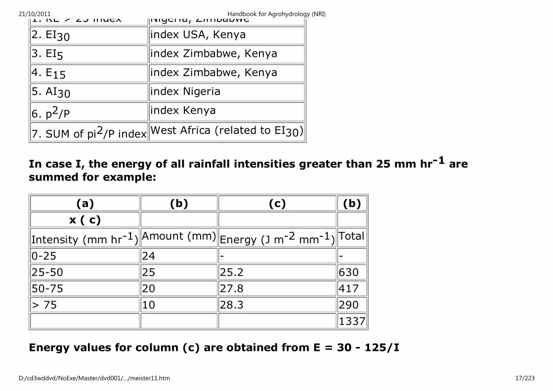
In case I, the energy of all rainfall intensities greater than 25 mm hr-1 are
summed for example:
(a) (b) (c) (b)
x ( c)
Intensity (mm hr-1) Amount (mm) Energy (J m-2 mm-1) Total
0-25 24 - -
25-50 25 25.2 630
50-75 20 27.8 417
> 75 10 28.3 290
1337
Energy values for column (c) are obtained from E = 30 - 125/I
21/10/2011 Handbook for Agrohydrology (NRI)
D:/cd3wddvd/NoExe/Master/dvd001/…/meister11.htm 17/223

In the cases of 2, 3 and 4 (EI indices) the subscript refers to the intensity period
in minutes. The energy values are obtained from E = 11.9 + 8.8 log I, then total
energy is multiplied by the intensity to give an erosivity value.
In example 5, the index is obtained from the total storm rainfall (A) and peak
intensity, I30. In 6 and 7, p is mean rainfall for the wettest month and P is mean
annual rainfall.
Examples of EI regression equations from Kenya are:
Soil loss in tonnes per hectare = 0.026 (EI15) - 1.18 with R2 = 0.71 and standard
error = 4.19
Soil loss = 0.35 (EI30) - 1 11 R2 = 0.69 se = 4.26
Soil Loss = 0.0054 (AI15) -1.35 R2 = 0.73 se = 4.07
3.1.2 Soil Erosion Control Practices
Soil erosion practices are widely known in agricultural practice and a brief
description is given of those most widely implemented.
a. Rotations
Rotations assist in erosion control by ensuring that soils are not exposed to the
same risks each season. Differing crop plant covers, growing period and rooting
densities, especially when periods of grass cover are incorporated, help to reduce
erosion and increase the binding organic matter content of soils.
21/10/2011 Handbook for Agrohydrology (NRI)
D:/cd3wddvd/NoExe/Master/dvd001/…/meister11.htm 18/223

b. Tillage
Tillage helps to increase infiltration and reduce runoff and soil loss, at least for a
short time. However, excessive tillage destroys the natural structure of soils and
exposes organic matter to oxidation. Thus a balance must be made between
sufficient tillage to achieve a good growing environment for crops and too much
tillage which can lead to soil crust development and enhanced runoff. Ploughing
depths should be varied to reduce the risk of a hard plough pan forming beneath
the soil surface.
c. Minimum and Mulch Tillage
Minimum tillage can give better erosion control and reduce costs compared to
conventional methods. Mulch tillage involves covering the soil surface with
suitable residues and can reduce runoff and soil losses considerably. It tends to
even out temperature differences and helps to protect the soil when plants are
small and cannot do so themselves.
d. Grazing Control
The control of stocking rates can be an extremely important factor in preventing
soil erosion by maintaining sufficient vegetation cover, preventing soil compaction
and thereby reducing runoff.
e. Water Conservation
Water control and conservation, which covers a wide range of practices: tillage,
cropping systems, farm planning and physical conservation techniques, is the
21/10/2011 Handbook for Agrohydrology (NRI)
D:/cd3wddvd/NoExe/Master/dvd001/…/meister11.htm 19/223

most effective way to reduce soil erosion. It amounts to an integrated approach to
land management.
Contouring: any farm operation carried out on the contour, ploughing, planting,
weeding, etc. may be regarded as contouring. Surface runoff is reduced by the
physical barriers thus formed which restrict the movement of water to small
distances and low velocities. Ridging increases its effectiveness, but field with
microtopography, drainage and gullies may be unsuitable, especially on high
slopes. Breakage of the features formed by contouring concentrates runoff and
increases soil erosion.
Strip cropping: this practice may be regarded as a type of contouring, but different
crops, grass or fallow are placed alternately on the contour to increase infiltration
and reduce runoff.
The design and construction of physical conservation practices (ridges, bunds,
terraces and flow channels) is covered in detail in chapter 7.
3.2 Field measurement of sediments (eroded material)
3.2.1 Total Sediment Collection
Equipment and Collection of Data
3.2.2 Suspended Sediment Samplers
Equal Transit Rate Method
Depth Integrated Sampling
21/10/2011 Handbook for Agrohydrology (NRI)
D:/cd3wddvd/NoExe/Master/dvd001/…/meister11.htm 20/223
Point Integrated Sampling
3.2.3 Pumping Samplers
Considering the site specific limitations of soil erosion models, it is perhaps not
surprising that erosion losses are still widely quantified by direct measurement.
The practical aspects of the measurement of eroded material are discussed below.
As with runoff studies, the selection of site locations will be largely determined by
their suitability to project objectives. From the agricultural point of view,
sedimentation and the loss of soil is the main focus of attention and in many ways
it is sensible to measure runoff and sediment at the same site and, where possible,
on the same experimental plots. Runoff plots are usually used to measure basic
erosion rates, or total sediment load, under specified soil/cover/ slope conditions,
and replication will probably be necessary. Total sediment loss measurements
obtained from small plots may not reflect real catchment conditions, because the
natural conditions of runoff loss and redistribution are imperfectly represented.
Natural catchment stream-gauging location points are usually suitable for
suspended sediment sampling, as are artificial controls emplaced on catchment
outlets. Little extra investment is needed to obtain sediment samples manually,
though laboratory facilities must be available for soil loss determination. Where
the site is remote and the cost can be justified, pumping sediment samplers are
sometimes used. A wide range of sampling devices are available and may be
adapted to suit local conditions. A number are described below.
3.2.1 Total Sediment Collection
21/10/2011 Handbook for Agrohydrology (NRI)
D:/cd3wddvd/NoExe/Master/dvd001/…/meister11.htm 21/223

Total sediment collection is obtained from the kind of runoff plot described in the
section on volumetric runoff data collection systems, in chapter 2. These systems
are constructed and operated exactly as described in the Runoff chapter, and the
design criteria of the tanks, peak flows and total volume are calculated in the
same way. The limitations of very small catchment size and regular site visits are
also the same. The data from these plots are important in agrohydrological
research and such erosion plots are commonly found on agricultural research
stations. Arrangements for ploughing, cropping will be made and bare or
uncultivated plots may be necessary to provide a controlled comparison. Natural
slopes are best suited to the collection of useful data, as reshaped areas will not
contain normal soil nor slope profiles.
Unlike most plots used for runoff measurement, the surfaces of plots which suffer
from high levels of erosion may become lower over several seasons and it is worth
considering whether or not to build in facilities that allow the collector gutter at
the downslope end of the plot to be lowered accordingly. The gradient of the pipes
leading to the collector tanks must be retained to prevent sediment collecting in
them (a velocity of 0.6 m s-1 is adequate). This may mean lowering the tanks
themselves, and during installation they should not be set in concrete, but put on
stands suitable to accommodate the lowering. Over-deep excavation of their
position may be necessary and this is often a laborious process necessitating the
use of heavy earth moving equipment. Chapter 2 gives details of construction,
installation and maintenance.
Samples taken from multislot and rotary dividers are expected to be
representative of the total runoff and the following equations may be used in the
calculation of sediment discharge.
21/10/2011 Handbook for Agrohydrology (NRI)
D:/cd3wddvd/NoExe/Master/dvd001/…/meister11.htm 22/223

GS =(QxC)/(Ax 103) where (3.9)
GS = Sediment discharge in kilograms ha-1
Q = Discharge in m³
C = Storm weighted concentration in ppm
A =Area of plot in hectares
Instantaneous sediment discharge rates can only be found if records of runoff
rates are available, that is if a control section and water level recorder are
installed on the catchment. If these data are available, then the formula to
calculate instantaneous sediment discharge 'g' is:
g = (q × C) / 103 where (3.10)
q = Instantaneous discharge rate in m³ s-1
C = Concentration in ppm by weight for runoff rate q
Sediments collected in the conduit and tanks of the runoff measuring equipment
are weighed in the field. Samples are taken as the material is weighed and the
percent of dry material is determined in the laboratory. Dry weight of the deposits
is given by:
Wsd = Wsw × Pdm where (3.11)
Wsd = weight of dry sediment
Wsw = weight of wet sediment
Pdm = percent dry material
21/10/2011 Handbook for Agrohydrology (NRI)
D:/cd3wddvd/NoExe/Master/dvd001/…/meister11.htm 23/223

Equipment and Collection of data
a. Multislot Dividers
For details of manufacture, installation and use of this equipment, see chapter 2. It
is likely that some runoff events will provide no soil material, perhaps because the
runoff plot is heavily vegetated or the rainfall is small. In these instances,
sedimentation data will not be available.
In cases where runoff provides sediment that can be suspended by stirring the
following procedure is followed:
- Agitation should be done energetically using flat paddles. It will probably
take two people.
- Fill three 1 litre sample containers, using a smaller container to fill them.
It is best to use 2 or 3 samples to fill each litre container so that examples
from the mix are selected.
- The containers should be pre-labelled to avoid accidental confusion with
date, time, plot, tank and sample no.
- The total measurement of runoff can then be taken, adding the 3 × 1 litre
samples to the total runoff amount.
- It is important to ensure agitation of the mix is continuous, so in total at
least three people will be necessary.
21/10/2011 Handbook for Agrohydrology (NRI)
D:/cd3wddvd/NoExe/Master/dvd001/…/meister11.htm 24/223

- This should be done for all tanks.
- As samples will have to be sent for analysis, it is important to check with
the laboratory that the required number of samples can be dealt with
conveniently. If not, it is probably best to reduce the overall number but
increase sampling dips, so as not to become involved with problems of
storage and the possibility that results will be late, samples lost or
accidentally destroyed. To a large extent this will depend on individual
circumstances, but it is an important point to note.
In cases where sediment is too heavy to be stirred totally into suspension, the
following procedure should be followed to collect samples:
- In the divider system described in chapter 2, the sludge will be trapped in
the first container in line.
- The supernatant (water and suspended) material should be removed to
within about 2 cm of the top of the sludge.
- This should be done carefully, with no disturbance of the deposited
material. It is likely that a syphon will have to be used rather than a pump,
which could suck up the deposited material.
- Allow more time for this procedure than would be needed for runoff
measurement alone.
- The sample bottles can be filled as the supernatant is siphoned and
measured for runoff volume
21/10/2011 Handbook for Agrohydrology (NRI)
D:/cd3wddvd/NoExe/Master/dvd001/…/meister11.htm 25/223

- Stir the sludge aggressively until it is liquid enough to find its own level.
- Measure its depth. It is necessary to ensure that the form of the
tank/container is known. This can be achieved by calibrating the volume of
the container for a given depth (using water), after installation. The
precision of calibration depends on the size of the tank, the advantage
being with smaller tanks, for which greater imprecision of depth
measurement gives smaller inaccuracies.
- Mix the sludge once more and during the process take the samples.
- Tanks and site should be left clean and free of debris.
b. Rotary Samplers
For details of manufacture, installation and use of this equipment, see chapter 2. -
Heavy sediment should be collected and weighed from the collection conduit and
transfer pipes. Tanks samples are taken as outlined above for multislot dividers.
3.2.2 Suspended Sediment Samplers
Suspended sediment samples are taken from water bodies such as streams and
reservoirs and do not involve the wholesale collection of runoff. However,
knowledge of the location of the source of material (other than it being
somewhere within the catchment), is difficult to obtain.
Suspended sediment samplers are designed to sample the sediment/water mix
and should ideally have the following features:
21/10/2011 Handbook for Agrohydrology (NRI)
D:/cd3wddvd/NoExe/Master/dvd001/…/meister11.htm 26/223

- They should sample with the intake at the same velocity as that of the
stream.
- They should sample away from the disturbance they cause.
- They should be able to sample close to the stream bed.
- They should be rugged and inexpensive.
In general it is probably best to purchase specially manufactured equipment,
though one set of such equipment could be used to calibrate the results of any
locally made equipment capable of fulfilling the criteria listed above.
There are two main types of samplers: depth and point integrating samplers.
The former instrument takes a continuous sample as it is lowered and raised from
and back to the water surface. Point samplers are equipped with an electrically-
operated valve which can be opened at desired depths and samples taken. If the
valve is left open, it will operate as a depth integrating device. These samplers are
streamlined bomb-shaped instruments, housing a glass bottle type sampling
container. The samplers can be used by wading in streams, but are often used on
rivers that necessitate the suspension of the instrument from bridges or cable
ways. Several sizes of sampler may be necessary where variations in flow volume
are present. The USDA gives recommendations on sampler types according to
speed of flow and depth (USDA handbook 224), but these relate only to equipment
obtained from within the US. Suspended sediment samplers are especially
important where runoff from river catchment areas is under study. Figure 3.2
shows a typical suspended sediment sampler
21/10/2011 Handbook for Agrohydrology (NRI)
D:/cd3wddvd/NoExe/Master/dvd001/…/meister11.htm 27/223

Figure 3.2: Suspended Sediment Sampler
The concentration of sediment within any flow is not only a function of the
physical characteristics listed earlier in the chapter, but also of time of flow. In
general, the rising limb of a hydrograph is prone to greater changes in
sedimentation as the runoff process gets underway and therefore requires more
frequent sampling. Similarly, small streams undergo a more rapid change in flow
stage than large streams and these too require more frequent sampling.
Table 3.5 gives guidelines for sampling frequencies, but it is important to
determine precise rates of sampling according to experience:
21/10/2011 Handbook for Agrohydrology (NRI)
D:/cd3wddvd/NoExe/Master/dvd001/…/meister11.htm 28/223

Table 3.5: Approximate Frequency of Sediment Sampling
Figure 3.3 shows the theoretical distribution of suspended sediment concentration
in a stream section, compared to the velocity distribution. Coarse, sand-sized
particles count for most of the variation in concentration, fine particles are usually
fairly evenly distributed throughout the stream section. As in many cases actual
concentrations vary with stage and turbulence, samples must be collected
systematically throughout the stream section.
21/10/2011 Handbook for Agrohydrology (NRI)
D:/cd3wddvd/NoExe/Master/dvd001/…/meister11.htm 29/223
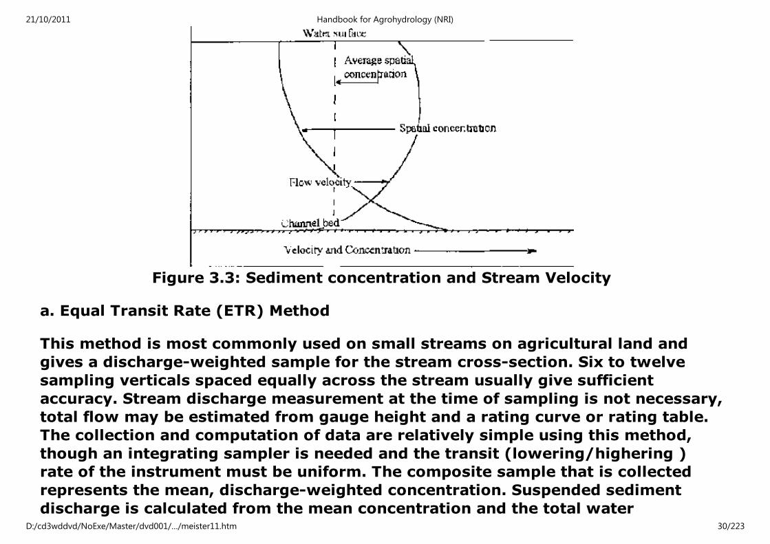
Figure 3.3: Sediment concentration and Stream Velocity
a. Equal Transit Rate (ETR) Method
This method is most commonly used on small streams on agricultural land and
gives a discharge-weighted sample for the stream cross-section. Six to twelve
sampling verticals spaced equally across the stream usually give sufficient
accuracy. Stream discharge measurement at the time of sampling is not necessary,
total flow may be estimated from gauge height and a rating curve or rating table.
The collection and computation of data are relatively simple using this method,
though an integrating sampler is needed and the transit (lowering/highering )
rate of the instrument must be uniform. The composite sample that is collected
represents the mean, discharge-weighted concentration. Suspended sediment
discharge is calculated from the mean concentration and the total water
21/10/2011 Handbook for Agrohydrology (NRI)
D:/cd3wddvd/NoExe/Master/dvd001/…/meister11.htm 30/223

discharge. Because it is commonly used, this method is covered in detail below.
Figure 3.4 shows the path of a sampler during a typical sampling procedure:
Figure 3.4
Path of Sampler During Equal Rate Sampling Procedure
- Select a straight section of stream, with as uniform a cross section as
possible, near the gauging station. Avoid shallow sections.
- Lay out a tape or line across the stream, standing downstream of the line
if wading.
- Determine the position of about 6 verticals (sufficient for a wadeable
stream of 10 m width)
- Record the stage of the stream.
- Rinse the sampler bottle, check for a clear orifice and stand about 1 m
down stream of the line at the first position to take the sample.
21/10/2011 Handbook for Agrohydrology (NRI)
D:/cd3wddvd/NoExe/Master/dvd001/…/meister11.htm 31/223

- Hold the sampler rod and move the sampler down at a constant speed,
touching the stream bed at each vertical.
- Sampling from surface to bed is recommended to avoid sampling
disturbed bed material at higher sampling points.
- The sampling velocity should not exceed 0.4 times the stream velocity.
- When a bottle becomes almost full, replace it and mark the sequence of
verticals and replacement .
- Usually between 1 and 6 bottles are needed.
- Record water temperature.
- Record stage if stream has fallen or risen significantly.
- It is convenient to put as much information on the bottle cap as possible
for ease of future sorting, but in any case ETR; the stream/catchment
name; date and time; stage; bottle sequence numbers; temperature and
signature should be written on the bottle label.
Where sandy bed streams are being sampled, a second sample run will reduce
sampling errors. Deeper streams can be sampled in a similar way, but a sampler
for use with line and winch equipment will be necessary. Different nozzles will
probably be available, so that the rate of collection of samples can be adjusted to
such prevailing stream conditions as depth and velocity. Charts are available that
indicate the speed of sampler transit and whether a single or two way transit is
21/10/2011 Handbook for Agrohydrology (NRI)
D:/cd3wddvd/NoExe/Master/dvd001/…/meister11.htm 32/223

recommended for particular nozzles, but the details will depend on manufacturer.
Errors that may be caused because of different flow velocities close to the stream
banks are not serious.
Where panicle-size analysis is to be undertaken, a second sample must be taken.
For all other methods, discharge must be measured at time of sampling.
b. Depth Integrated Sampling
A relatively large number of depth integrated samples must be taken on verticals
at the midpoint of equal sections of the width of the stream. Usually 6 to 12 are
sufficient, each located within cross-sections of equal discharge. Mean sediment
concentration is found by weighting the mean concentration in each sampling
vertical with respect to the discharge in the vertical.
Total suspended sediment is found by mean cross section concentration and total
water discharge. Discharge must be measured at the time of sampling. Variations
in sediment concentration across the stream may be obtained. Alternatively, the
collection of depth integrated samples at verticals that represent the middle of
sections of equal discharge may be undertaken.
c. Point Integrated Sampling
Samplers used in this method are equipped with an electrically operated valve
which takes samples on command. With the valve continuously open, they perform
in a manner similar to depth integrating samplers. Point samples are taken in
stream verticals which represent equal or known discharge. Mean values are
weighted accordingly, but the number of points depend on the physical character
21/10/2011 Handbook for Agrohydrology (NRI)
D:/cd3wddvd/NoExe/Master/dvd001/…/meister11.htm 33/223

of stream flow.
In general, the ETR method (a.) is most widely used.
3.2.3 Pumping Samplers
These samplers are complex pieces of equipment and relatively costly to obtain
and install. It is probable that their cost can only be justified if soil erosion studies
are a major activity of a project and if suspended sediment sampling from streams
is an important component of this activity. Pumped samples do not represent
discharge weighted samples as they are point measurements. Therefore,
calibration curves that plot pumped samples against discharge weighted samples
(taken simultaneously) must be compiled until a known relation is established.
These must be revised should the relation change with time.
They are located in a shelter at the side of the stream and take samples of the
flow, a portion of which is retained. They are useful for remote locations where
site staff cannot be stationed. Samples are collected and stored in bottles. An
intake is placed in the stream and typically a float activated, battery powered
system comes into operation at a predetermined stream level. Samples are
pumped into bottles at selected, predetermined time intervals until the stream
level falls or the containers are full. Most of the pumped water goes to waste, to
remove any debris drawn in by the previous sampling process, samples only being
taken at the end of the pumping period. It is usual to site the equipment at a
gauging station so that an indicating mark can be made on the water level
recorder chart, when sampling takes place. Records of stage and sampling are
thus linked. Some systems rely on a gravity feed sampling and are usually sited at
21/10/2011 Handbook for Agrohydrology (NRI)
D:/cd3wddvd/NoExe/Master/dvd001/…/meister11.htm 34/223

such locations as reservoirs and weir installations.
Bed samples may be collected from perennial streams using special sampling
dredgers, sampling cores and spuds but in most cases the costs of such equipment
will not be justified by the information returned. Deposits of bed sediment may be
sampled by soil sampling cores for the determination of bulk density and chemical
analysis, during the dry season.
The mapping and surveying of channels, changes in gullies and the upslope
movement of gully scarps can be important aspects of erosion and sedimentation
studies. Mapping is required in great detail
3.3 Laboratory analysis
3.3.1 Sediment Concentration
Evaporation Method
Filtration Method
Separating Fines and Sands
Particle Size Analysis
Pipette Method
Hydrometer (Bouyoucos) Method
Wet Sieving
Dry Sieving
The analysis of samples will probably be undertaken at a specialist laboratory, but
this is an expensive procedure and may even involve the dispatch of samples to
another country. Therefore descriptions of common analysis techniques are given
21/10/2011 Handbook for Agrohydrology (NRI)
D:/cd3wddvd/NoExe/Master/dvd001/…/meister11.htm 35/223

below. In some cases analyses can be undertaken with relatively simple
equipment and is possible even where orthodox laboratory facilities are not
available, if costs can be met. Evaporation and filtration are the two usual
methods of determining sediment concentration. As it is more convenient to work
with weights rather than volumes concentrations are usually determined as a ratio
of dry sediment weight to sediment/water mixture. Conversion to units of
milligrams per litre or parts per million is undertaken afterwards.
Packing and Transport of Soil and Water Samples
The most suitable container for a soil sample is a thick polythene bag which can
be sealed with tape. This can then be put into a second paper or cloth bag for
extra protection. For all analyses except bulk density, there is no problem if the
sample is disturbed. Samples of about 1 kg are suitable, large stones having been
removed. Where gravel content is of interest the sample may be 2-3 kg. Very wet
samples may be dried, but any mixture of samples or contamination should be
avoided. Samples should be placed in small wooden or cardboard boxes for
transport as soon as possible to the laboratory; the addition of tuline to kill
organisms may be necessary if samples are to be tested for nitrate and cannot be
delivered promptly.
Water samples should be carried in screw-top polythene bottles and placed in
boxes that are fitted with sections to separate each bottle from the next. Any
empty space in packing cases or boxes should be packed with wadding to prevent
movement of the samples during transport. Samples of 1 litre are adequate and
soda glass containers should be used if an analysis for boron is to be undertaken.
21/10/2011 Handbook for Agrohydrology (NRI)
D:/cd3wddvd/NoExe/Master/dvd001/…/meister11.htm 36/223

Water and soil sample containers should be clearly marked, at least twice, with a
water proof pen. So should any outer container. Details of samples should be
recorded in a sample book and generally the less detail on the sample the better,
to avoid confusion, however a detailed packing note should accompany any
container of samples. It may be necessary to check with the laboratory in case it
has a preferred system of labelling.
3.3.1 Sediment Concentration
a. Evaporation Method
Basic equipment is as follows:
- Graduated containers 0.5 -1.0 litre capacity.
- Large container, 5 litres or more
- Distilled water
- Vacuum source
- Evaporation dishes of several sizes
- Convection drying oven
- Pipette
- Desiccator
- Flocculating agent
- Balances accurate to 0.1 gram and 0.1 milligram
The procedure is as follows:
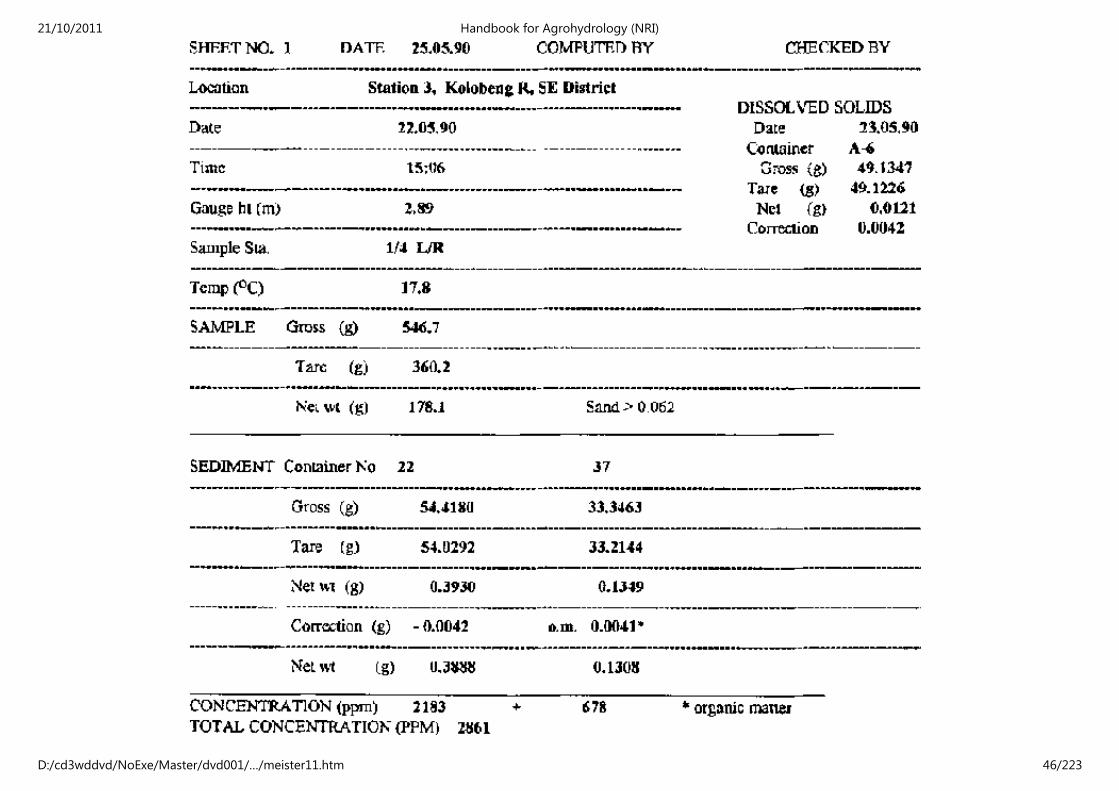
- Prepare a worksheet (see Figure 3.5)
21/10/2011 Handbook for Agrohydrology (NRI)
D:/cd3wddvd/NoExe/Master/dvd001/…/meister11.htm 37/223

- Transfer all sample details from the bottles to the work sheet.
- Weigh the total sample, less the container(s) weight(s) and record.
- If the colloidal material is in suspension, flocculate adding 0.40 millilitre
of 0.2 molar solution of alum (90.7 g l-1).
- Allow the sample to settle overnight or for at least 12 hours.
- Note that flocculant is not usually used for concentrations < 1000
milligrams per litre. If this is done then the introduced error can be
calculated for example: 50 milligram per litre solution added to a
concentration of 1000 milligrams per litre will give an error of 5%, if all the
flocculant is sorbed by the sediment.
- If samples have relatively little colloidal clay, they can be allowed to
settle for a few hours and no flocculant is needed.
- Using the vacuum source and appropriate tubing, remove all water except
30 millilitres from the sample. This amount can be approximate, so long as
it is the same amount for all the samples. All the effluent from the samples
from one sampling site can be combined in one large container.
- Wash the remaining sample into a numbered evaporation dish with
distilled water.
- Place in the oven and dry overnight at 105 - 110°C. It is best to avoid
vigorous boiling and splashing of the sample. The sample container can be
21/10/2011 Handbook for Agrohydrology (NRI)
D:/cd3wddvd/NoExe/Master/dvd001/…/meister11.htm 38/223

used where possible.
- Remove from the oven and place in the desiccator, weigh as soon as
possible after removal.
- Enter gross and tare weights and obtain net weight of sample on the
worksheet.
- Mix effluent thoroughly and withdraw 100 millilitres. Oven dry at 105 -
110°C, weigh sample enter on the worksheet.
- Compute the correction factor for the effluent by dividing the net amount
of dissolved solids (the residue) by the aliquot volume (in this case 100
millilitres) and multiply the volume of water left in the large sample
container × 1 million. (0.3888 g / 178.1 g) × 106 = 2183 ppm
To compute the concentration in milligrams per litre:
Concentration = B × ( weight of sediment × 106/ weight of water-sediment
mixture) in mg l-1.
The value of the factor 'B' can be obtained from Table 3.6 which is based on
specific weights for water and sediment of 1.000 and 2.65 g cm-3.
21/10/2011 Handbook for Agrohydrology (NRI)
D:/cd3wddvd/NoExe/Master/dvd001/…/meister11.htm 39/223

21/10/2011 Handbook for Agrohydrology (NRI)
D:/cd3wddvd/NoExe/Master/dvd001/…/meister11.htm 40/223

Figure 3.5: Example Worksheet for Evaporation Method of Sediment Concentration
Compute sediment concentration (in parts per million) as follows. Figure 3.5, the
worksheet, provides the example:
Subtract correction factor from the net sediment weight. In Figure 3.5 for
example.
0.3930 g - 0.0042 g = 0.3888 g
Divide oven dry weight of the sample by the net sample weight of the sediment
plus water and multiply by one million.
Table 3.6: Values of Factor 'B' for the Computation of Sedimentation Concentration
in mg l-1 When Used with Ratio (x 106) of Weight of Sediment to Weight of
Water/Sediment Mixture (0-29°C)
21/10/2011 Handbook for Agrohydrology (NRI)
D:/cd3wddvd/NoExe/Master/dvd001/…/meister11.htm 41/223

b. Filtration Method
The filtration method works well with low sediment concentrations and obviates
the need for the dissolved solids correction. Compile a work sheet as shown in
Figure 3.6
Equipment is as follows:
- Got crucibles, at least 25 millilitre capacity with perforated bottom,
suitable to be fined to a vacuum system.
- Filters. Commercial glass fibre or cellulose are satisfactory for most
sediments.
- Distilled water
- Vacuum system
- Evaporation dishes of several sizes
- Convection drying oven
- Desiccator
- Flocculating agent
- Balances accurate to 0.1 gram and 0.1 milligram
Set up as follows:
21/10/2011 Handbook for Agrohydrology (NRI)
D:/cd3wddvd/NoExe/Master/dvd001/…/meister11.htm 42/223

- Determine the weight of the sediment/water mixture (the sample).
- Allow to settle until clear then decant the excess liquid into another
beaker.
- Install suitable filter into crucible and determine tare weight.
- Connect crucible to vacuum system and transfer sample.
- When filtration is complete place crucible into oven and dry at 105 -110
°C.
- Remove and place in desiccator. Remove and weigh and compute
concentration. Other methods of filtration can be used.
- A simple glass funnel fitted with a filter paper, the sample draining under
gravity can be used when samples have a relatively high colloidal content
and if care is taken.
Procedure:
- Follow the first three steps of the evaporation method.
- Wet sieve the material using sample water.
- Remove the material < 0.062 mm.
- Dry and weigh this material.
21/10/2011 Handbook for Agrohydrology (NRI)
D:/cd3wddvd/NoExe/Master/dvd001/…/meister11.htm 43/223

- Remove the material > 0.062 mm (sands) and put in a tared evaporation
dish.
- Oven dry and weigh.
- Adjust to pH 3 - 5 with HCl, using pH paper.
- Add about 1 millilitre of 30 percent H2O2 (hydrogen peroxide) per gram
of dry sample, in 40 millilitres of water.
- Allow to stand to oxidise the organic material (this will take a few hours)
and remove any floating organic material.
- Destroy any remaining organic material and hydrogen peroxide by
bringing the sample to a boil.
- Oven dry sand sample and weigh.
- Determine the organic content by subtracting the gross weight of sands
from gross weight of sands before peroxide treatment and record.
- Record gross and tare sand weights on worksheet, compute net sand
weight and record.
- Subtract weight of organic matter from weight of sand and record. No
correction for dissolved solids is necessary as the effluent was washed into
the fines portion during sieving.
21/10/2011 Handbook for Agrohydrology (NRI)
D:/cd3wddvd/NoExe/Master/dvd001/…/meister11.htm 44/223

- Compute sands and fine concentrations as described in the Evaporation
method. Total concentration is equal to sum of fines and sands.
21/10/2011 Handbook for Agrohydrology (NRI)
D:/cd3wddvd/NoExe/Master/dvd001/…/meister11.htm 45/223
21/10/2011 Handbook for Agrohydrology (NRI)
D:/cd3wddvd/NoExe/Master/dvd001/…/meister11.htm 46/223

Figure 3.6 Example Worksheet Filtration Method
c. Separating Fines and Sands
The separation of fines and sands is frequently used in analysis and is normally
made at 0.062 mm, though different preferences can be catered for. The
equipment is the same as the Evaporation method, with the addition of a 0.062
mm (or 0.053 mm) meshed sieve. Figure 3.7 gives an example worksheet.
Procedures:
For the sands:
- Follow the first three steps of the Evaporation method
- Wet sieve on the 0.062 mm sieve using sample water.
- Remove material < 0.062 mm. Dry and weigh to the nearest 0.1 ma.
- Adjust to pH 3 -5 with HCl using pH paper.
- Add about 1 millilitre of 30 percent H2O2 per gram of dry sample in about
40 ml of water.
Allow to stand to oxidise the organic matter.
- Destroy hydrogen peroxide by boiling
- Oven dry sample and weigh to nearest 0.1 ma.
- Determine organic content by deducting weight of sample after from
before hydrogen peroxide treatment.
- Record gross and tare sand weights, compute net sand weight.
- Subtract organic matter weight from sand weight and record.
21/10/2011 Handbook for Agrohydrology (NRI)
D:/cd3wddvd/NoExe/Master/dvd001/…/meister11.htm 47/223

- Compute sand and fines concentrations as for Evaporation method.
- Total concentration is found by totalling concentrations of sands and
fines.
21/10/2011 Handbook for Agrohydrology (NRI)
D:/cd3wddvd/NoExe/Master/dvd001/…/meister11.htm 48/223

Figure 3.7: Example Worksheet Sands and Fines
21/10/2011 Handbook for Agrohydrology (NRI)
D:/cd3wddvd/NoExe/Master/dvd001/…/meister11.htm 49/223

For the fines:
- Continue with the steps of the Evaporation method
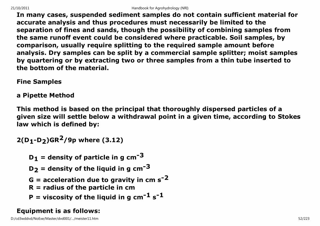
3.3.2 Particle Size Analysis
Particle size analysis is undertaken not only for sedimentation work, but also to
determine soil textural type. Several methods may be employed because of the
wide range of particle sizes frequently present in samples. Table 3.7 gives size
range, analysis concentration quantity of sediment and methods of analysis,
recommended by the USDA SCS. Table 3.8 gives a grade scale of sediment particle
sizes.
Table 3.7 Recommended Particle Size Analyses
21/10/2011 Handbook for Agrohydrology (NRI)
D:/cd3wddvd/NoExe/Master/dvd001/…/meister11.htm 50/223

Table 3.8 Soil Textural Classes and Particle Sizes
The most commonly used methods of analysis are:
Fine sediments: Pipette, Hydrometer and Bottom Withdrawal (B W) Tube
Methods. The former two methods are most commonly used and are
detailed below.
Coarse sediments: Sieving and the Visual Accumulation Tube Methods.
Details of these methods are given below.
21/10/2011 Handbook for Agrohydrology (NRI)
D:/cd3wddvd/NoExe/Master/dvd001/…/meister11.htm 51/223
In many cases, suspended sediment samples do not contain sufficient material for
accurate analysis and thus procedures must necessarily be limited to the
separation of fines and sands, though the possibility of combining samples from
the same runoff event could be considered where practicable. Soil samples, by
comparison, usually require splitting to the required sample amount before
analysis. Dry samples can be split by a commercial sample splitter; moist samples
by quartering or by extracting two or three samples from a thin tube inserted to
the bottom of the material.
Fine Samples
a Pipette Method
This method is based on the principal that thoroughly dispersed particles of a
given size will settle below a withdrawal point in a given time, according to Stokes
law which is defined by:
2(D1-D2)GR2/9p where (3.12)
D1 = density of particle in g cm-3
D2 = density of the liquid in g cm-3
G = acceleration due to gravity in cm s-2
R = radius of the particle in cm
P = viscosity of the liquid in g cm-1 s-1
Equipment is as follows:
21/10/2011 Handbook for Agrohydrology (NRI)
D:/cd3wddvd/NoExe/Master/dvd001/…/meister11.htm 52/223

- 25 millilitre pipette apparatus (see Figure 3. 8 below)
- A vacuum source.
- Sedimentation cylinders of 1,000 millilitre capacity with rubber bungs.
- Stirring rods, brass of 6.4 mm diameter by 61 cm with a perforated plastic
disc 5 cm in diameter, attached to end.
- Thermometers, Evaporating dishes.
- Desiccators, Stopwatch.
- Worksheets, 0.062 mm sieve.
Predetermined depths and times of withdrawal are given below in Table 3.9, based
on the assumptions that particles have a spherical shape and a specific gravity of
2.65. The viscosity of the fluid is assumed to vary from 0.010087 cm²s-1 at 20 ° C
and 0.008004 cm²s-1 at 30 °C. The gravitational constant is 9.80 m s-2.
Procedure:
If an organic matter and soluble salts content is required, the supernate is
removed, the sample dried and weighed before these items are removed.
Otherwise the first step is to remove any organic material by oxidation.
- Use HC1 to adjust the sample pH to 3 - 5 for oxidation.
21/10/2011 Handbook for Agrohydrology (NRI)
D:/cd3wddvd/NoExe/Master/dvd001/…/meister11.htm 53/223

- Add about 1 millilitre of 30% H2O2 for each gram of dry sample. Stir and
allow to stand for several hours.
- Any floating material can be removed.
- Usually samples need to be heated (less than 70°C) and more H2O2
should be added.
- When the reaction has stopped, the sample is boiled or washed with
distilled water to remove the H2O2.
The second step is to remove soluble salt material.
- Effervescence, evident when a little dilute HCl is added to the sample
indicates the presence of carbonates.
- To remove them, add 50 millilitres of a slightly acid sodium acetate (Na O
Ac) buffer solution ( Na C2 H3 O2 3H2O,1N, 136 g l-1 adjusted to pH 5 with
acetic acid) to each 5 grams of sample.
- Bring to suspension by stirring with a rubber tipped glass rod. Digestion
is helped by heating the beaker in a water or sand both at near boiling
temperature.
- After 30 minutes the suspension is washed by filtering with a filter candle
(= to Pasteur-Chamberian or Selas type FP porcelain candle, 02 or 03
porosity). Some samples may need two or more treatments.
21/10/2011 Handbook for Agrohydrology (NRI)
D:/cd3wddvd/NoExe/Master/dvd001/…/meister11.htm 54/223
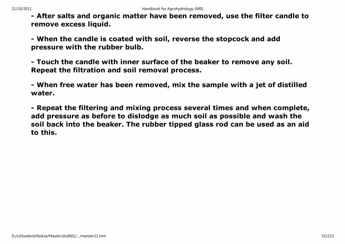
- After salts and organic matter have been removed, use the filter candle to
remove excess liquid.
- When the candle is coated with soil, reverse the stopcock and add
pressure with the rubber bulb.
- Touch the candle with inner surface of the beaker to remove any soil.
Repeat the filtration and soil removal process.
- When free water has been removed, mix the sample with a jet of distilled
water.
- Repeat the filtering and mixing process several times and when complete,
add pressure as before to dislodge as much soil as possible and wash the
soil back into the beaker. The rubber tipped glass rod can be used as an aid
to this.
21/10/2011 Handbook for Agrohydrology (NRI)
D:/cd3wddvd/NoExe/Master/dvd001/…/meister11.htm 55/223

Table 3.9: Time of Pipette Withdrawal for Given Temperature, Depth of Withdrawal
and Diameter of Particle
21/10/2011 Handbook for Agrohydrology (NRI)
D:/cd3wddvd/NoExe/Master/dvd001/…/meister11.htm 56/223

Figure 3.8: Schematic Diagram of Pipette Method Equipment
Thereafter analytical procedures are as follows:
- If both concentration and particle size are needed, weigh the
water/sediment to the nearest 0.1 gram before proceeding.
- Remove excess water with a filter candle and place sample in a tared
evaporation dish, dry at 100 -110° C and weigh to the nearest milligram.
- Deflocculate by adding a dispersing agent (40g sodium
hexametaphosphate (Na P03)6 and 8 grams sodium carbonate in distilled
water to 1 litre) for each 5 to 10 grams of sample.
- Transfer to a 250 millilitre shaker beaker adding distilled water to bring
the volume to 180 millilitres, shake overnight. More convenient is the use
21/10/2011 Handbook for Agrohydrology (NRI)
D:/cd3wddvd/NoExe/Master/dvd001/…/meister11.htm 57/223

of a mechanical analysis stirrer which will complete the mixing in 2 -5
minutes.
21/10/2011 Handbook for Agrohydrology (NRI)
D:/cd3wddvd/NoExe/Master/dvd001/…/meister11.htm 58/223

Figure 3.9: Worksheet for Pipette Method
In some cases, for example where the concentration of suspended sediments is
very low, dispersion may not be necessary. Where it is, the dissolved solids
correction must be determined for each new solution of the dispersing agent as
follows:
- Add 10 millilitres of dispersing agent to a calibrated sedimentation
cylinder, dilute to volume with distilled water, mix thoroughly and remove
25 millilitres, transfer to an evaporation dish and dry overnight at 105 -
110 ° C, weigh the dish and contents to the nearest 0.1 milligram.
- Perform in triplicate and use the average. The net weight of the dissolved
solids is subtracted from the net weight of each pipette withdrawal.
Continue as follows:
- Weigh each sedimentation cylinder while empty then fill to between 500
and 1000 millilitres with distilled water. Weigh again several times and use
the average. Do the same for the 25 millilitre pipettes. The ratio of mean
weight of water in the cylinder: mean weight of water in the pipette is used
as a volume ratio in comparing the results of the withdrawals.
21/10/2011 Handbook for Agrohydrology (NRI)
D:/cd3wddvd/NoExe/Master/dvd001/…/meister11.htm 59/223

- Select particle size determinations and using Table 3.9 set up a schedule
for time and depth of withdrawals.
- Use distilled water to wet sieve (0.062mm) the dispersed sample, passing
material into a sedimentation cylinder. Place the sands into a tared
evaporation dish and dry, weigh to the nearest 0.1 milligram for the net
weight.
- When ready to pipette, bung the cylinder and shake vigorously while
turning end over end then plunge with the brass stirring rod.
- Immediately lower the pipette 10 cm into the sample and take a "zero
time" withdrawal. Take the temperature and plunge again for 1 minute.
After this make withdrawals according to the depth/time schedule, always
measuring the sampling depth from the existing surface of the suspension.
- Each time, the pipette is flushed with distilled water and with the
withdrawn sample, this is put into numbered and tared evaporating dishes.
A rubber bulb may be used to blow out remaining droplets.
- Oven dry the withdrawals overnight (100 - 110 ° C) cool in a desiccator
and weigh to the nearest milligram to determine net weight. Results may
be tabulated as in Figure 3.9.
Calculations are carried out as follows:
- From the "zero time" withdrawal determine the net weight of fines in the
sample and record. Make a dissolved solids correction if a dispersing agent
21/10/2011 Handbook for Agrohydrology (NRI)
D:/cd3wddvd/NoExe/Master/dvd001/…/meister11.htm 60/223
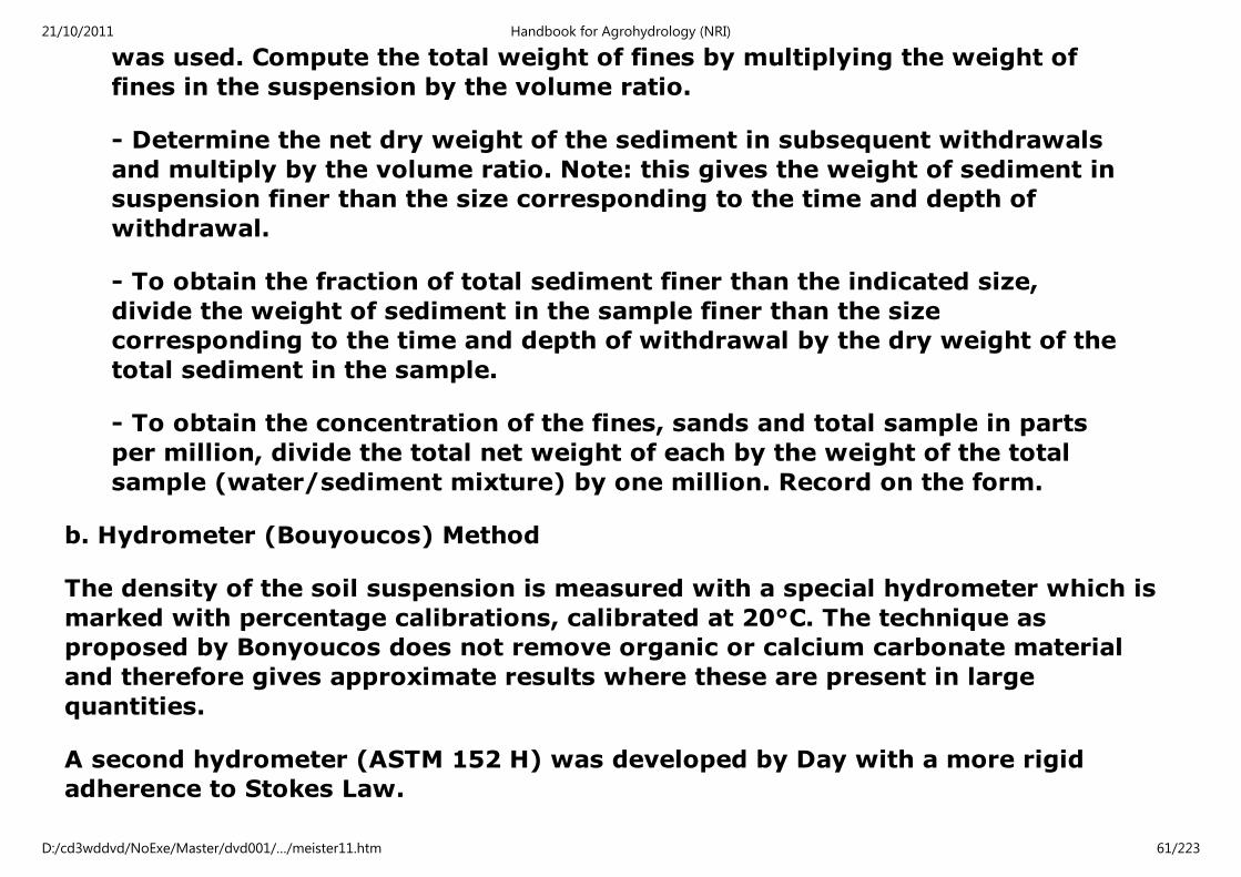
was used. Compute the total weight of fines by multiplying the weight of
fines in the suspension by the volume ratio.
- Determine the net dry weight of the sediment in subsequent withdrawals
and multiply by the volume ratio. Note: this gives the weight of sediment in
suspension finer than the size corresponding to the time and depth of
withdrawal.
- To obtain the fraction of total sediment finer than the indicated size,
divide the weight of sediment in the sample finer than the size
corresponding to the time and depth of withdrawal by the dry weight of the
total sediment in the sample.
- To obtain the concentration of the fines, sands and total sample in parts
per million, divide the total net weight of each by the weight of the total
sample (water/sediment mixture) by one million. Record on the form.
b. Hydrometer (Bouyoucos) Method
The density of the soil suspension is measured with a special hydrometer which is
marked with percentage calibrations, calibrated at 20°C. The technique as
proposed by Bonyoucos does not remove organic or calcium carbonate material
and therefore gives approximate results where these are present in large
quantities.
A second hydrometer (ASTM 152 H) was developed by Day with a more rigid
adherence to Stokes Law.
21/10/2011 Handbook for Agrohydrology (NRI)
D:/cd3wddvd/NoExe/Master/dvd001/…/meister11.htm 61/223

The original hydrometer method was devised to provide a quick and easy method,
the accuracy of which could be established by comparison with pipette analyses
and thereafter be used with confidence. The modifications introduced by Day
increase accuracy, but the analysis is no longer rapid (it takes about as long as the
pipette method) and it is essential that organic matter and calcium be removed by
pretreatment.
Bouyoucos Method
Equipment:
Apparatus and reagents as for pre-treatments and separation of sand
Mixing plunger
Thermometer including the 15 - 25 °C range
Accurate clock or stop watch
Bouyoucos or ASTM hydrometer
Hydrometer jars marked at 1 litre
Procedure:
- Estimate whether sample is sandy (silt and clay < 15%) or not sandy. In
first case transfer 100 g oven dry sample to 250 ml beaker and add 100 ml
5 percent solution of hexametaphosphate-sodium carbonate. In second use
50 g.
- Rest overnight, transfer to mechanical stirrer, washing out the beaker and
making up the volume to 500 ml with water.
21/10/2011 Handbook for Agrohydrology (NRI)
D:/cd3wddvd/NoExe/Master/dvd001/…/meister11.htm 62/223
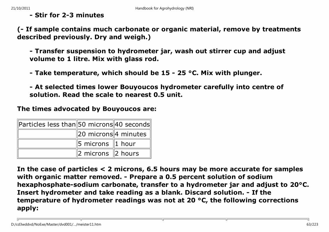
- Stir for 2-3 minutes
(- If sample contains much carbonate or organic material, remove by treatments
described previously. Dry and weigh.)
- Transfer suspension to hydrometer jar, wash out stirrer cup and adjust
volume to 1 litre. Mix with glass rod.
- Take temperature, which should be 15 - 25 °C. Mix with plunger.
- At selected times lower Bouyoucos hydrometer carefully into centre of
solution. Read the scale to nearest 0.5 unit.
The times advocated by Bouyoucos are:
Particles less than 50 microns 40 seconds
20 microns 4 minutes
5 microns 1 hour
2 microns 2 hours
In the case of particles < 2 microns, 6.5 hours may be more accurate for samples
with organic matter removed. - Prepare a 0.5 percent solution of sodium
hexaphosphate-sodium carbonate, transfer to a hydrometer jar and adjust to 20°C.
Insert hydrometer and take reading as a blank. Discard solution. - If the
temperature of hydrometer readings was not at 20 °C, the following corrections
apply:
Temperature Correction (g per Temperature Correction (g per
21/10/2011 Handbook for Agrohydrology (NRI)
D:/cd3wddvd/NoExe/Master/dvd001/…/meister11.htm 63/223
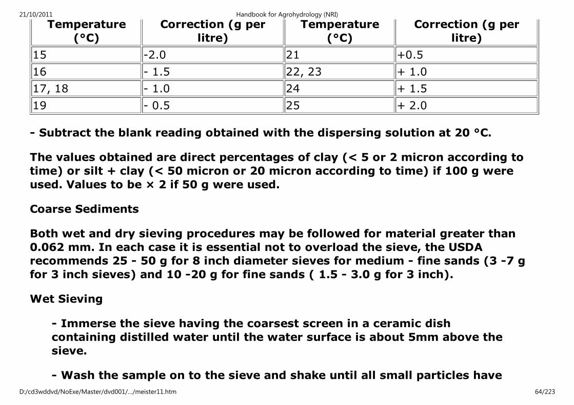
Temperature
(°C)
Correction (g per
litre)
Temperature
(°C)
Correction (g per
litre)
15 -2.0 21 +0.5
16 - 1.5 22, 23 + 1.0
17, 18 - 1.0 24 + 1.5
19 - 0.5 25 + 2.0
- Subtract the blank reading obtained with the dispersing solution at 20 °C.
The values obtained are direct percentages of clay (< 5 or 2 micron according to
time) or silt + clay (< 50 micron or 20 micron according to time) if 100 g were
used. Values to be × 2 if 50 g were used.
Coarse Sediments
Both wet and dry sieving procedures may be followed for material greater than
0.062 mm. In each case it is essential not to overload the sieve, the USDA
recommends 25 - 50 g for 8 inch diameter sieves for medium - fine sands (3 -7 g
for 3 inch sieves) and 10 -20 g for fine sands ( 1.5 - 3.0 g for 3 inch).
Wet Sieving
- Immerse the sieve having the coarsest screen in a ceramic dish
containing distilled water until the water surface is about 5mm above the
sieve.
- Wash the sample on to the sieve and shake until all small particles have
21/10/2011 Handbook for Agrohydrology (NRI)
D:/cd3wddvd/NoExe/Master/dvd001/…/meister11.htm 64/223

passed through.
- Pass the material and washing water onto the next smallest sieve and
continue to repeat the process until the smallest sieve is reached.
- Transfer the material on to a tared container, dry and weigh each fraction.
Any material passing through the 0.062 sieve is to be analysed by other
methods
Dry sieving
- Set a nest of sieves on a mechanical shaker, coarsest on top, proceeding
to the finest.
- Weights for each fraction are determined after about 10 minutes of
shaking.
Equipment costs
All costs of locally made equipment are approximate. The costs of raw materials
and especially labour are highly variable from country to country, but a good idea
of cost magnitude can be gained from the figures quoted below. The costs of
manufactured equipment are based on 1993 prices. Shipping costs, agents fees
and fluctuations in exchange rate cannot be taken into account.
21/10/2011 Handbook for Agrohydrology (NRI)
D:/cd3wddvd/NoExe/Master/dvd001/…/meister11.htm 65/223
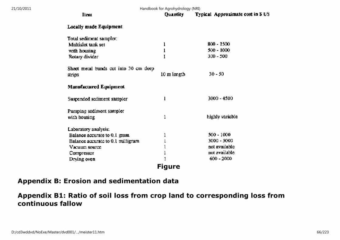
Figure
Appendix B: Erosion and sedimentation data
Appendix B1: Ratio of soil loss from crop land to corresponding loss from
continuous fallow
21/10/2011 Handbook for Agrohydrology (NRI)
D:/cd3wddvd/NoExe/Master/dvd001/…/meister11.htm 66/223

Appendix B1 part I
21/10/2011 Handbook for Agrohydrology (NRI)
D:/cd3wddvd/NoExe/Master/dvd001/…/meister11.htm 67/223

Appendix B1 part II
21/10/2011 Handbook for Agrohydrology (NRI)
D:/cd3wddvd/NoExe/Master/dvd001/…/meister11.htm 68/223
Home"" """"> ar.cn.de.en.es.fr.id.it.ph.po.ru.sw
Handbook for Agrohydrology (NRI)
Chapter 4: Rainfall and other meteorological data
4.1 Rainfall
4.2 Other meteorological data
Equipment costs
Handbook for Agrohydrology (NRI)
Chapter 4: Rainfall and other meteorological data
4.1 Rainfall
The collection of snowfall data is not covered here. If detailed information is
needed, consult a handbook such as USDA No. 224 or approach the local
meteorological service. Ordinary, standard gauges with the collection/funnel
component removed and a measured amount of antifreeze added can be used to
measure snowfall, but errors due to wind effects can be very large.
Rainfall is the most important single factor in determining whether runoff will or
21/10/2011 Handbook for Agrohydrology (NRI)
D:/cd3wddvd/NoExe/Master/dvd001/…/meister11.htm 69/223

will not occur for a given set of environmental conditions. It determines runoff
amount and frequency. There are two measurements of rainfall amount that are
commonly collected for hydrological purposes: Daily and (runoff) Event rainfall.
Daily Rainfall is probably the most ubiquitously measured meteorological variable.
It is the rain that falls awing a 24 how period starting in the morning of one day
(commonly 06:00, 07:00 or 08:00 furs) until measurement is made at the same
time the following day. Event Rainfall by contrast is the rainfall occurring awing an
unspecified time period usually, but not always less than 24 hours, that can be
seen to be responsible for subsequent runoff. The collection and use of each has
advantages and disadvantages.
In the case of daily rainfall, data are usually available from many stations, even in
countries with only the most basic meteorological network. The equipment to
measure daily rainfall is relatively cheap, simple to install, read and maintain. All
projects should easily achieve adequate instrumentation. In most cases, many
years of historical data will be available for analysis from a variety of sources, in
addition to that obtained from meteorological offices: these sources include
various government departments, water resource and construction projects, state
and private farms, schools and interested individuals. Often basic analyses will
have been performed on the data (average monthly and annual totals, spatial
distribution, etc.). For the analysis of runoff relations, however, daily rainfall can
have one serious drawback. It is the lump sum rainfall awing a 24 how period and
in some climatic environments may greatly exaggerate the amount of rainfall
thought to be responsible for runoff, but despite this drawback, it is the most
commonly used climatic variable in runoff studies.
21/10/2011 Handbook for Agrohydrology (NRI)
D:/cd3wddvd/NoExe/Master/dvd001/…/meister11.htm 70/223

Event rainfall, obtained from the careful examination of the records of an
automatically recording rain gauge, can provide a precise and accurate evaluation
of the rainfall responsible for runoff and it is often to be preferred for
rainfall/runoff analyses. However, recording rain gauges are not usually in
widespread use except at important synoptic stations (especially in developing
countries). They are expensive to buy, can be difficult to maintain and staff must
have a higher level of expertise to operate them. The analysis of data is more
complex and time-consuming.
It is possible to determine whether or not daily rainfall and runoff event rainfall
are for all practical purposes, the same, though a number of historical data are
necessary to do this. Values of daily rainfall are plotted against values of runoff
event rainfall, as illustrated in Figure 4.1. A visible correlation exists for these data
from sites around Gaborone in SE Botswana, confirmed by the statistical
significance of the coefficient of determination of the relation (R2 = 0.99) The
gradient of the line which is for all practical purposes 1:1, the regression equation
being y= 1.025x + 0.068. In this case, daily rainfall values could be used instead
of event rainfall, without fear of inaccuracy. The ratio of Daily to Event rainfall may
not be 1:1, but any relation that is highly significant can be used. Where the
relation is not significant, daily rainfall cannot be used to estimate the actual
rainfall that caused runoff. The similarity between daily and event rainfall depends
on climatic regime but it will be more evident in areas that have convective
rainfall, giving heavy, short periods of rain and many thunderstorms. The analysis
of rainfall data is discussed in greater detail in Chapter 8.
Rainfall Intensity defines the amount of rain falling during a specified time within
the most intense period of the rain. This value is then converted into the amount
21/10/2011 Handbook for Agrohydrology (NRI)
D:/cd3wddvd/NoExe/Master/dvd001/…/meister11.htm 71/223

of rain that would fall in one how at this intensity. For example if 5 mm of rain
falls in a 2 minute period, the 2 minute duration rainfall intensity is 150 mm hr-1
and if 27 mm falls in 30 minutes, the 30 minute duration rainfall intensity is 54
mm hr-l. Rainfall intensity can have an important effect on runoff proportion, as it
determines the rate at which rain arrives at the soil surface and, consequently,
whether the infiltration rate of the soil is sufficient to allow absorption. Automatic
recording gauges are needed to measure rainfall intensity The duration under
study will be determined to a large extent by catchment size; small plot runoff is
often closely related to the 2 or 5 minute intensity durations while large
catchment relations are more evident with long durations. The use of daily rainfall
becomes a more attractive proposition under these circumstances, especially as
the use of long duration intensities can lead to a serious reduction in data, when
rainstorms are short-lived.
21/10/2011 Handbook for Agrohydrology (NRI)
D:/cd3wddvd/NoExe/Master/dvd001/…/meister11.htm 72/223

Figure 4.1: The Relation Between Daily Rainfall and Event Rainfall
4.1.1 Non-Recording (Daily) Rain Gauges
All agrohydrological projects will collect daily rainfall from manually read rain
gauges. Even when automatic recording gauges are installed it is important to
cross-check the amounts that they measure and ensure that at least daily values
are collected if they develop faults. Some automatic gauges have integral manual
gauges sited under the recorder to facilitate this. Different models of daily rain
21/10/2011 Handbook for Agrohydrology (NRI)
D:/cd3wddvd/NoExe/Master/dvd001/…/meister11.htm 73/223
gauges are used in different countries. In the case of some developing countries,
which can ill-afford even basic meteorological equipment, national networks may
use more than one type, having been supplied by different aid agencies or having
inherited them from various projects. Usually this does not cause serious
problems. It is essential however, to ensure that the correct measuring vessel into
which the rain is poured from the gauge (and calibrated only for one particular
model) is used to measure the rainfall amount. As a general rule, it is sensible to
purchase equipment compatible to that already used by the national
Meteorological Service. This has several advantages:
- Data will be strictly compatible.
- In the case of loss or breakage of measuring vessels (glass), a temporary
loan may be possible.
- The Service will be familiar with procurement/replacement procedures.
- The Service will be familiar with the most suitable methods of
installation.
- Service staff and other gauge readers who may be called upon to read the
gauges, will be familiar with the equipment. In some cases it may even be
possible to arrange the loan of gauges, if the Service has sufficient reserve.
Types of Gauge
Any open ended vessel can be used as a rain gauge, but uniformity of design to
provide consistent splash characteristics necessitates the use of purchased
21/10/2011 Handbook for Agrohydrology (NRI)
D:/cd3wddvd/NoExe/Master/dvd001/…/meister11.htm 74/223

equipment. Most gauges are made of corrosion-resistant metal such as brass.
Gauges with orifices of different sizes measure rainfall with about the same
degree of accuracy. Results of tests show that readings are within 1% from gauge
openings of between 5 to 50 cm. Differences in measurement usually result from
installation and reader error rather than gauge design.
The standard US Weather Bureau non-recording gauge has an 8 inch (20.3 cm)
orifice, the UK standard gauge (commonly adopted by former colonies) has a 5
inch (12.7 cm) opening. There is little to choose in design accuracy, but in general,
smaller gauges tend to be less expensive. Figure 4.2 shows examples.
21/10/2011 Handbook for Agrohydrology (NRI)
D:/cd3wddvd/NoExe/Master/dvd001/…/meister11.htm 75/223

Figure 4.2 Non-recording Rain Gauges.
Non-recording gauges usually consist of a collector above a funnel which passes
collected rain into a receiving vessel. Important requirements are that the
collector walls should be vertical inside and steeply bevelled outside. It should
prevent rain splashing in or out by having a sufficiently deep wall and a funnel
with steep sides (at least 45 degrees). The area of orifices should be consistent.
The receiving vessel should have a narrow neck (to prevent evaporation losses).
It is usual to use a larger vessel in the same gauge, where it is impractical to visit
the gauge on a daily basis.
21/10/2011 Handbook for Agrohydrology (NRI)
D:/cd3wddvd/NoExe/Master/dvd001/…/meister11.htm 76/223
The measuring (calibration) vessel should be of clear glass with engraved
graduations (usually at 0.1 mm intervals). The type of gauge that it is to be used
with, should be clearly marked. To achieve accurate readings for small rainfall
amounts, the base will be tapered. Dip rods are sometimes used instead of
measuring vessels, but this is unusual.
Plastic rain gauges, often inverted cones in shape and marked with mm
gradations, are available in some countries and can provide a good, cheap
alternative to expensive standard rain gauges. However, three important facts
should be recognized.
- They eventually degrade due exposure to UV light, after one or two
seasons.
- They cannot be recommended in areas of frequent hard frost.
- Not all such gauges are produced to accurate specifications and the
accuracy of the gradations should be checked and if necessary, calibrated
before use.
- They are difficult to install with the orifice exactly horizontal, using a
single post.
Installation of Non-recording Gauges
The location of the gauge is the primary consideration in obtaining accurate
rainfall measurements and the most serious problem is wind turbulence.
Buildings, trees, fences produce eddies and reduce accuracy. Isolated obstructions
21/10/2011 Handbook for Agrohydrology (NRI)
D:/cd3wddvd/NoExe/Master/dvd001/…/meister11.htm 77/223
should not be closer than twice their height to the gauge (further away if
possible). However, openings in woods and orchards are suitable places (so long
as the trees are no closer than specified); they act as windbreaks and reduce
violent air currents. Sloping ground should be avoided and surrounding vegetation
should be cut low. In general, smooth artificial surfaces are not suitable as they
tend cause splashing and may attain high surface temperatures.
It is very important that the height above ground level of gauge orifices should be
the same at all sites. It is preferable that the orifice be as close to the ground as
possible. Wind velocity increases with height and the catch of the gauge is
reduced thereby underestimating rainfall, however gauges positioned at ground
level are prone to in-splashing, which is also undesirable. The UK Meteorological
Office recommends that gauges' orifices be located at 305 mm above ground level
as a compromise to minimise both of these effects. The influence of wind on rain
catch can be expected to be greater in areas of convective rainfall where air
turbulence is inherent.
In difficult field conditions however, the practical limitations of accidental
disturbance and vegetation growth can result in problems with gauges set close to
ground level. From experience, a suitable height is between 0.8-1.2 m. In this
range of heights the gauge should be clearly visible and vegetation growth
between visits from project staff should not affect readings. A consistent height
for all gauges based on local field conditions is probably more important than
following hard and fast recommendations. Ground-level gauges can be seen at
meteorological stations, but here constant attention can be given to vegetation
clearance, animals should not be a problem and checks can easily be made on the
equipment. This may not be so at field sites.
21/10/2011 Handbook for Agrohydrology (NRI)
D:/cd3wddvd/NoExe/Master/dvd001/…/meister11.htm 78/223
The stand supports that hold the gauge should be inexpensive, strong, durable,
rigid and easy to build from local materials. Wood is best avoided due to
susceptibility to termites and rot. Materials should be easy to transport into the
field. Although a concrete base in which stand legs can be set or bolted seems
sensible and is often advocated, in areas where animal damage is possible, it is
better to install the stands with metal pegs or by digging the legs into the ground
to an depth of 50 cm, which is usually adequate. This may lead to the toppling of a
gauge if pushed by cattle, but it can be reset immediately and will not be out of
operation until the stand is replaced and re-cemented. In all cases, the gauge
should be set horizontally by testing with a spirit level.
Gauges may often be placed on private land and it is essential to obtain
permission from the owner before doing so. Usually a discussion as to the aims of
the project, the (realistic) long-term benefits that are hoped for, and the purpose
of the gauge are sufficient to obtain permission. Sometimes and if suitable, land
owners can be recruited as gauge readers. It is important to provide an enclosure
for the rain gauge to reduce the risk of damage from animals and to prevent
interference with normal land use. Barbed wire is most suitable, with strands
placed closer together (10-15 cm apart) at the bottom. Not only does this prevent
access to animals and deter vandals, but also has no discernible effect on rainfall
catch. Cut thorntree branches (e.g. Acacia species) woven into the lowest metre of
the fence are a good deterrent against goats and other agile animals, although in
areas of termite activity this will need to be replaced each season. For the same
reason, enclosure posts are best made of metal, though they are more expensive
than wood. If they are too costly or unavailable, wooden posts will last several
seasons if soaked in creosote or other preservative. In some areas, termite-
resistant tree species can be found for use.
21/10/2011 Handbook for Agrohydrology (NRI)
D:/cd3wddvd/NoExe/Master/dvd001/…/meister11.htm 79/223
Even though wind turbulence is important in reducing rain gauge accuracy, the
use of windshields can generally be discounted. Their main aim is to reduce wind
speed, turbulence and splash over the gauge and allow siting close to the ground,
but in practice they are not easy to make locally and increase problems of
interference by people and animals. Research has shown that differences in
shielded and unshielded gauges are relatively small (2-8%).
When locating rain gauges in the field it is important to keep in mind the problems
of theft and vandalism. Prevention can be aided by the provision of fencing and
enclosures, but the safest action is to enlist the help of local people. Sites placed
by the homes of gauge readers are usually convenient and secure. When
positioned in more public places, such as common village land, it is advisable to
discuss the purpose of the equipment at an open meeting, where the use of rainfall
data can be explained. An agreement for safe custody of the equipment can
(usually) be made without difficulty.
The UK Met Office and US Weather Bureau recommend that rain gauges in exposed
positions be located within a circular turf wall to negate the effects of wind
turbulence. Figure 4.3 illustrates the construction of the protective wall which
should be kept in a good, clean condition. Note that the rain gauge orifice is level
with the top of the wall. It should be stated that in many circumstances, recourse
to such a structure will be very difficult.
21/10/2011 Handbook for Agrohydrology (NRI)
D:/cd3wddvd/NoExe/Master/dvd001/…/meister11.htm 80/223

Figure 4.3 Construction of Turf Wall to Remove the Effect of Wind
Non-Recording Rain Gauges: Routine Data Collection and Site Staff
At field sites that do not have automatic recording gauges, locally-hired gauge
readers will almost certainly be required and it is essential that a good working
relationship be established and maintained with such gauge readers, observers or
site guards. More difficulties in the collection of field data arise from people than
from instruments and reliable field staff are an invaluable asset to any project. The
selection of suitable field staff can be difficult and common sense and judgement
of personality are important criteria in arriving at a suitable choice. The
opportunities to recruit will vary from country to country and will depend on
social as well as educational factors. The following points can help.
- The person should be reliable and suited for the job. They should be
literate and numerate at least to a basic level. It is unlikely that they will
need skills sufficient to understand instrument manuals (this can actually
be a disadvantage if they are "zealous" in the performance of their duties),
but they will be using printed record sheets and measuring and recording
numerical values.
21/10/2011 Handbook for Agrohydrology (NRI)
D:/cd3wddvd/NoExe/Master/dvd001/…/meister11.htm 81/223

- Village school teachers are often used as recorders of rainfall, by national
meteorological services. However, they have other responsibilities and
often take holidays away from their village. Rainfall records often suffer as
a result.
- If possible, it is useful to have someone who can speak your own
language, or an interpreter will always be necessary.
- A permanent resident is preferable, even if less educated. Their new
responsibilities should not be in conflict with their normal day-to-day
business.
- Be aware that the recruitment can give rise to discontent within the
family/community by imparting status and/or financial gain to the
individual.
- It is important to resist the recruitment of individuals who may be using
their status within the community to acquire more and/or who expect
financial gain, without being prepared to carry out the work properly.
- The gauge reader should be able to reach the gauge easily, therefore they
should live close by and have permission for access if it is sited on
someone else's land.
- After selection, the reader should be given a thorough explanation of why
the data are being collected and the importance to the village and project.
- They should be tested for competence in all their responsibilities.
21/10/2011 Handbook for Agrohydrology (NRI)
D:/cd3wddvd/NoExe/Master/dvd001/…/meister11.htm 82/223

A contract should be drawn up covering all duties and rewards in a simple but
comprehensive list. For example:
- Reading the gauge at specified times (check that this can be done, or at
least that the time of reading can be noted).
- Keeping the record book and measuring vessel at a specified place so that
they can be checked on field visits.
- Cleaning the gauge when necessary.
- Noting damage to the gauge, enclosure and keeping down vegetation etc.
- Repairing any such damage when possible.
- Keeping the site clear of vegetation on a routine basis.
- Informing in advance the use of the deputy and expected departures from
site.
- Basic pay, holidays or pay in lieu.
- Deductions or action in the event of neglect of duties.
- Best method of contact in the case of unforeseen events.
Any seasonal changes in these duties should be stated, as should a clause
covering unsatisfactory performance. A suitable deputy should be appointed as it
is inevitable that at some time the gauge reader will have to leave the site. The
21/10/2011 Handbook for Agrohydrology (NRI)
D:/cd3wddvd/NoExe/Master/dvd001/…/meister11.htm 83/223
contract should be translated into the local language if necessary. It is best if
payment is made for the services of the gauge reader. This puts the arrangement
on a business footing and no favours are asked by either side.
Payment should reflect local employment conditions, bearing in mind that while
the work is not arduous, it does restrict the mobility of the gauge reader. All
payments should be recorded, copied and signed for without failure. Most of these
points will be influenced by local conditions, but a friendly involvement by the
project field staff in the reader's work coupled with a direct and business-like
approach seem to get best results.
The maintenance of non-recording gauges is straight forward and should be
carried out by the gauge reader. The gauge should be checked for any blockage
(cobwebs, insects, leaves etc.) in the funnel at each reading by holding the orifice
component to the light. Even partial blockages should be cleared. The collection
vessel should seen to be watertight and clean and the felt washer on the funnel of
the gauge which fits over the vessel mouth (and helps to prevent evaporation)
intact. The measuring (calibration) vessel should be clean and in good repair. It is
useful to have a spare at site as these are made of glass. It should be ensured that
the gauge is correctly seated on or in its stand, often gauges are disturbed when
the tightly-fitting collection component is removed to measure the rainfall
21/10/2011 Handbook for Agrohydrology (NRI)
D:/cd3wddvd/NoExe/Master/dvd001/…/meister11.htm 84/223

Figure 4.4: Routine Data Collection Sheet, Non-Recording Rain Gauges
The stand should be checked for stability and deterioration and repairs effected if
necessary. The area around the gauge should be kept clear of vegetation and the
enclosure fence kept in good condition. Any repairs to or re-instatement of the
gauge, including the date of original installation should be noted in the record
book. The field team should carry a book identical to the site record book, with the
same headings and columns, so that information can be copied from one to the
other with minimum error. A hardback notebook, protected from the weather with
stitched pages (rather than a file with loose, detachable pages) is best. Columns
to be set out in a form similar to those in Figure 4.4, in addition to the name and
address (and telephone number if appropriate) of the project, contact name etc.
being clearly printed, in more than one language if necessary, on the book.
21/10/2011 Handbook for Agrohydrology (NRI)
D:/cd3wddvd/NoExe/Master/dvd001/…/meister11.htm 85/223

Field teams should routinely carry certain items such as a tool kit for impromptu
repairs to gauges and stands (depending on the types used), spare record book,
spare measuring glass, pay sheets, etc.
It is important to remember that meteorological offices "throw back" daily rainfall
records, i.e. to attribute rainfall recorded on a morning to the previous day. This
may not be appropriate for some studies.
4.1.2 Recording (Intensity) Rain Gauges
There are three main types of recording rain gauge systems: Tipping bucket,
Syphon and Weighing. Recent advances have led to the use of electronic loggers
which now frequently replace the usual chart and pen clockwork systems.
Alternatively, very compact intensity gauges measuring to a precision of 1 mm of
rain and reputedly accurate to 2% over 2 years are available, though the cost of
this equipment is not low. A liquid crystal display readout is given via a
connecting cable and daily, weekly and monthly accumulated totals may be
collected.
a. Tipping Bucket Gauge
These are commonly seen as in Figure 4.5, below. There are many different types
and the manufacturers manual must be followed carefully, as is the case for all
recording rain gauges. A dual tipping bucket pivots on a horizontal axis which lies
beneath the funnel of the orifice, such that only one bucket receives rainfall at a
time. When filled to a preset, calibrated amount (for example 0.2 mm) the bucket
tips and is emptied, leaving the second bucket to receive rain. Tips are recorded
21/10/2011 Handbook for Agrohydrology (NRI)
D:/cd3wddvd/NoExe/Master/dvd001/…/meister11.htm 86/223

electronically and individually.
Data are downloaded and analysed by computer software, though hard copies
used for manual analysis are sometimes available via a portable printer carried to
the field. Alternatively, the data may be recorded on a mechanically driven chart.
In general the tipping mechanism works well, but sometimes does not register
very light rain in hot climates. It may also under-register during very intense
storms, because of the finite time taken for the buckets to exchange positions.
Electronic logger type
Advantages:
- Simple download directly to a computer.
- With computer programs, the analysis of intensity data is quick and easy.
- No problems with mechanical clock, ink, pen etc.
- Very large amounts of data can be stored (32 - 120 kb)
- Options for storing data, time, etc. only when rain occurs, thereby saving
memory.
- Can operate for very long periods.
Disadvantages:
- Some designs are new and may not be well field tested.
21/10/2011 Handbook for Agrohydrology (NRI)
D:/cd3wddvd/NoExe/Master/dvd001/…/meister11.htm 87/223

- If the logger or battery fails, then all the data can be lost.
- Needs computer facilities at base (good electricity supply, etc.).
- Needs spare loggers or portable computer, both of which are expensive.
Maintenance
Buckets must move freely and be oiled on a regular basis in some cases.
Mechanism must be checked frequently to ensure that it is horizontal.
Battery and connections must be tested at each visit and replacements made when
necessary. Gauges come precalibrated, but they must be re-calibrated at the end
of each season in the laboratory. This is a simple process whereby known volumes
are emptied into the gauge from a pipette and checked against the record. Check
with the manufacturer's instructions.
The tipping motion closes an electrical contact (usually current is provided by a 6
volt dry battery) which registers a pulse on an electrical counter or logger, each
pulse representing the bucket contents (the example 0.2 mm of rain). The data are
usually in the form of each tip represented by a time (Month: Day: Minute:
Second). The opportunity to record the gauge name/number may or may not be
offered, so it is wise to keep a careful note of from where the logger came. A
'record only with rain' facility is usual.
Various methods of down-loading can be used. In some instances the logger must
be removed and taken to base to be down-loaded via an interface and computer. A
replacement must be provided. In some cases the data can be downloaded in to a
portable computer and the logger can remain at site. In all cases some sort of set-
21/10/2011 Handbook for Agrohydrology (NRI)
D:/cd3wddvd/NoExe/Master/dvd001/…/meister11.htm 88/223

up procedure is necessary to re-activate the logger once the data are extracted.
Figure 4.5: Tipping Bucket Raingauge, Electronic Logger Type
Mechanical (Clockwork drum and chart)
Some gauges provide a chart record of the tipping instead of an electronic
recorder. A permanent pen record is kept of each tip on a clock driven drum chart.
Clocks usually work for about 30 days without attention, but this can be altered in
most cases, by replacement of parts of the gearing mechanism.
Advantages:
- Permanent record is kept on chart, therefore cannot be lost.
- Less likely to be affected by adverse conditions
21/10/2011 Handbook for Agrohydrology (NRI)
D:/cd3wddvd/NoExe/Master/dvd001/…/meister11.htm 89/223

Disadvantages:
- Analysis of data is lengthy and must be entered manually into computer
storage.
- Needs more frequent visits
- Not as flexible in terms of alteration of the instrument settings
Some recorders offer both electronic and mechanical records. This gives a good
back-up facility and some models even record river levels simultaneously. In some
cases the tipped water runs to waste, but some gauges have the provision for the
rainfall to be collected in a vessel below the gauge via a funnel and so the total
rainfall for the period between readings is known. This can be very useful if the
gauge or logger develop problems.
Maintenance
This is a little more complicated than for the electronic gauges, though the bucket
check is the same. Clock accuracy must be tested on a regular basis, even though
charts last 30 days without attention. Chart replacement should be done with an
accurate pen reset and any malfunction noted. Chart drum motor may be
clockwork or electrical.
b. Tilting Syphon Type
Versions of this type suitable for use in tropical countries are available. Figure 4.6
illustrates a typical syphon instrument.
21/10/2011 Handbook for Agrohydrology (NRI)
D:/cd3wddvd/NoExe/Master/dvd001/…/meister11.htm 90/223

Rain is collected and falls into chamber A, and raises float B. In response, the pen
moves upward and its trace is recorded on the chart fixed to the drum, H. The
chamber is on a pivot (C), over-balances when full and empties through the
syphon tube (D). The pen is then reset to the zero position while lifted clear of the
chart by the rod G. The over- balancing is controlled by the trip, E and the
chamber is restored to its original position by F, the counterweight. The siphoning
takes approximately 15 seconds.
Figure 4.6: Tilting Syphon Rain Gauge
It is important to test the mechanism regularly by pouring in water through the
inlet and to keep the syphon tube and its gauze filter clear of blockage at all times.
21/10/2011 Handbook for Agrohydrology (NRI)
D:/cd3wddvd/NoExe/Master/dvd001/…/meister11.htm 91/223

c. Weighing Type
This type is less common than the former kinds, but is especially useful where
snow is frequently experienced. Precipitation is collected from a funnel into a
bucket which, as the frame upon which it stands falls with increasing collection,
stretches an isoelastic spring. The movement of the frame is proportional to
precipitation and linked to a pen by a series of levers. This records on a clock-
driven drum chart.
The maintenance of recording gauges will be the responsibility of visiting field
teams who must be trained to a higher level than the field gauge reader
responsible for daily gauges. Tools, loggers, charts, pens and ink will be carried
routinely. Although gauges are of a type (syphon, tipping bucket, mechanical,
electronic etc.), each will vary according to the manufactures' particular
specifications and it is impossible here to list specific instructions for all gauges.
In addition to the points of particular care noted in the sections describing the
types of recording raingauge, the manufacturers instruction manuals should be
carried to the field and studied carefully.
Factors Affecting Accuracy of Rain gauges
Many factors affect the accuracy of rain gauges. These include evaporation,
adhesion, inclination of the gauge, condensation and splash. However, these are
unlikely to cause differences of more than about +/- 1%, whereas wind
turbulence at a poorly sited and maintained station can account for much larger
errors. The precise effects of wind speed is still contentious despite many years of
research. Some authors predict large deficits (for example 17% with winds of 16
21/10/2011 Handbook for Agrohydrology (NRI)
D:/cd3wddvd/NoExe/Master/dvd001/…/meister11.htm 92/223

km hr-1 and 60% at 48 km hr-1) while others (see Figure 4.7 below) expect the
effect of wind speed on rain gauge catch to be much less. Agreement that wind
effects cause an underestimate of rainfall (and more especially snowfall) is
universal, however.
Damage to the instrument during carriage should be avoided, especially denting
about the orifice, which can cause discrepancies in readings. Splits and cracks in
the receiving vessel can cause serious losses. Care should be taken to ensure that
all the water is emptied into the measuring vessel and that the measurement is
made accurately at the bottom of the meniscus.
Figure 4.7: Catch versus Wind Speed
A list of errors and causes inherent in measuring rainfall from standard, non-
recording gauges are given below. Other factors, notably poor maintenance, faulty
resetting of loggers, pens and charts can affect the accuracy of rainfall records
21/10/2011 Handbook for Agrohydrology (NRI)
D:/cd3wddvd/NoExe/Master/dvd001/…/meister11.htm 93/223

obtained from intensity gauges.
Figure 4.8: Errors in the Observation of Point Rainfall
Rain Gauge Networks
Many projects will be adequately served by the installation of rain gauges at each
experimental site, when the interpolation of data between sites is unnecessary or
can be easily achieved, perhaps using data from the national network. In some
circumstances it may even be best to install two daily gauges, to allow for
occasions when one gauge may be accidentally inoperative, though of course this
must be balanced against cost. If the site area is large, these should be separated,
with one gauge in the centre of the site and one at its boundary. When placed on a
line at right angles to the prevailing wind, it is sometimes possible to collect
information on the distribution of rainfall. If resources allow, the installation of a
recording rain gauge at each site, in addition to at least one non-recording gauge,
is to be preferred for agrohydrological purposes. Rainfall intensity is an important
influence on runoff and its study will undoubtedly play an important part in the
research agenda. However, recording rain gauges are very expensive (even "low
cost" data-logger versions are currently several hundred pounds sterling, each)
and project resources must be considered carefully.
If resources are inadequate for total coverage by recording gauges, then partial
cover must be budgeted for. The success of partial cover will depend on a sound
21/10/2011 Handbook for Agrohydrology (NRI)
D:/cd3wddvd/NoExe/Master/dvd001/…/meister11.htm 94/223
instrumentation strategy, which can only decided upon by the staff of each
individual project. This will be dependent on the number of sites, their proximity
to the base station and each other, the spatial variation of rainfall characteristics,
the time between visits and field staff reliability. The two extreme options are:
1. to place all recording instruments at the most distant stations. This will
provide event, daily and intensity data from widespread, infrequently
visited sites which would otherwise give only rainfall totals from several
days using non-recording gauges. However, it is wise to recognise that
infrequently visited sites are always the most troublesome. Faults in and
damage to the equipment will not be seen for some time, gauges can be
interfered with or even stolen. Data and equipment could be totally lost.
Access may be impossible at times during the wet season.
2. The second extreme option is to place all such valuable equipment at or
near the base station. There is little danger of problems with the equipment
not being rectified quickly, but the opportunity to collect data from diverse
areas is lost. The best solution, clearly, lies between these two examples
and to some extent trial and error (especially becoming familiar with the
reliability of the gauges under field conditions) will be needed to determine
which outlying stations are most suitable. It is essential to monitor one
gauge carefully at the base station and check its readings and reliability of
operation.
In many areas of convective rainfall, a statistical randomness means that over
time, the average number of storms of a given intensity will be experienced at all
locations within the study area. Thus it is reasonable to presume that rainfall
21/10/2011 Handbook for Agrohydrology (NRI)
D:/cd3wddvd/NoExe/Master/dvd001/…/meister11.htm 95/223

intensity can be extrapolated from one site to another, if certain characteristics of
a rainstorm (for example the amount and duration of rain) are known. It is
convenient if a statistically significant relation exists between rainfall amount and
rainfall intensity and allows the substitution of one type of data for another. Figure
4.9 below shows 30 minute duration rainfall intensity against daily rainfall. The
significance exceeds the 99.9% level. In some instances, a clustering into groups
of data points may be seen with a strong correlation among them, probably
indicating that different types of rainfall (for example low intensity frontal and
high intensity local convectional) have been experienced. The 2 minute duration
intensity against daily rainfall showed no significant relation for the data.
If a comprehensive raingauge network is proposed for an agrohydrological
project, the number and density of instruments will depend on several factors.
Those relating to the physical environment are:
- Size of area covered
- Prevailing storm type
- Topography and Aspect
- Variation in seasonal rainfall
In general, more gauges will be needed for large areas and denser networks will
be needed where storms are convective and localised with high intensities (as
opposed to cyclonic areas where rainfall tends to be widespread and of more
uniform, low intensity). Convective rainfall is characterised by the predominance
of thunderstorms. Mountainous areas, which create orographic rainfall, are
21/10/2011 Handbook for Agrohydrology (NRI)
D:/cd3wddvd/NoExe/Master/dvd001/…/meister11.htm 96/223

expected to have localised rainfall regimes and to need a more dense network
than plateau areas (Table 4.1). However in practice, the rainfall in mountainous
areas may be of a more regular distribution than extremes of elevation may
suggest whereas flat plains dominated by very local convective rain storms often
exhibit very large coefficients of variation of rainfall distribution.
It is important to plan with the hydrological characteristics of the area in mind.
For instance it is more important to place a denser network of gauges in areas
which contribute most to runoff, than in homogeneous areas which contribute
little. It is possible to use correlation analysis in determining network densities.
For instance if the correlation of daily rainfall between adjacent gauges is high
(say, r = 0.90 or greater), a firm basis is provided to reduce the number of gauges
in the network. Rainfall is spatially variable to a high degree and even the densest
network of gauges can provide no more than an estimate of areal precipitation.
Networks are best planned in the preliminary stage of a project by the use of a
map desk study to provide a picture of the overall pattern of gauge distribution.
The distribution should not be random; random events are studied by a systematic
arrangement of sampling points. Minor revisions of the network pattern can be
made during installation, if unexpected problems of siting are found. It is useful to
place some gauges outside the study area to ensure that extrapolation is possible
to the boundaries of the study area. More gauges are needed if results are to be
taken to other areas, rather than limited to the original study area.
21/10/2011 Handbook for Agrohydrology (NRI)
D:/cd3wddvd/NoExe/Master/dvd001/…/meister11.htm 97/223

Figure 4.9: Daily Rainfall versus Rainfall Intensity
As stated above, project objectives and resources will determine, to a great
extent, the level of instrumentation. A watershed study that relates total
precipitation and total annual runoff yield would need fewer gauges than a study
of rainfall on a storm-by-storm basis. The USDA regards the following gauge
densities as suitable (see Table 4.1), but states clearly that the size of the study
area is the only criterion used to determine them. Factors such as climate and
21/10/2011 Handbook for Agrohydrology (NRI)
D:/cd3wddvd/NoExe/Master/dvd001/…/meister11.htm 98/223

topography are not considered. These recommendations can be compared to those
of WMO which take into account, in a limited way, climate and topography.
However, it is likely that the needs of the project will be of paramount importance
when compared to such general recommendations.
Table 4.1 Recommended Density of Daily Rain Gauges by Size of Study Area
4.2 Other meteorological data
Rainfall data collected for hydrological purposes will also be useful to other
project members, such as agronomists and soil physicists. The same is true of
other meteorological data which may be important, for example in assessing crop
performance under varying climatic conditions. These other data will help
categorise climate in general and are essential to estimate evapotranspiration and
soil moisture conditions which can have an important effect on runoff production,
soil moisture availability and crop growth. Indeed, the calculation of
evapotranspiration is one the most important uses to which comprehensive
21/10/2011 Handbook for Agrohydrology (NRI)
D:/cd3wddvd/NoExe/Master/dvd001/…/meister11.htm 99/223

climatic data are put during agrohydrological investigations. This chapter
concentrates on instrumentation; the uses and analysis of data are covered in
chapter 8.
Site of Meteorological Stations
The installation of climatic instruments requires a suitable site which should be
representative of the macroclimate of the study area. Where climate varies
greatly, perhaps due to topography, several stations may be necessary, though the
spatial variability of some meteorological variables is greater than others. The site
should not be in an exposed position on a steep slope, nor should it be within the
distance of four times the height of any nearby trees or buildings. In semi-arid
areas, sparsely vegetated open areas make good, representative sites. The site
will probably represent the greatest concentration of instruments for a project and
it is essential that a suitable, secure location be selected. Advice on
instrumentation should be sought from the local Meteorological service and where
possible instruments of the same manufacture should be acquired.
The site can be instrumented according to particular need, but special attention
should be paid to such details as shading from elevated posts and other
instruments. Doors to equipment should be away from direct sunlight, areas of
artificial surfaces should be kept to a minimum. The area should be well fenced
and gated, not higher than 1m, with wire mesh which is fine at the foot of the
fence, to deter animals. Birds can be prevented from roosting on instruments by
the provision of alternative high perches. Fence posts should be of metal to avoid
termite damage. It is useful to retain extra space within the compound, for
instruments that may be added at a later date. Where possible recording
21/10/2011 Handbook for Agrohydrology (NRI)
D:/cd3wddvd/NoExe/Master/dvd001/…/meister11.htm 100/223

instruments should be used. Experience will show that records obtained manually,
during holidays and weekends often appear suspiciously inconsistent when
compared to weekday readings.
Records of equipment should be kept secure at the station. Loose-leafed books are
more prone to damage and loss than those with permanent bindings. A site map of
water pipes, cables etc. is useful if the station acquires permanent buildings.
Longitude and latitude should be noted on any such map. Records of instruments
added or removed are very useful as are schedules for routine repair, painting and
grass mowing. Files should be kept which contain notes on the instruments; when
bought, invoices, serial numbers, calibration tests, instruction manuals, repairs
etc. Having this information easily at hand can save a great deal of time and
frustration. Such details should be kept separate from the day-to-day records of
measurements, and in a secure place.
4.2.1 Air Temperature
Air temperature is one of the most commonly measured meteorological variables.
Maximum and minimum temperatures are used to calculate mean daily values for
use in evapotranspiration estimations. Figure 4.10 illustrates the installation of
maximum/minimum thermometers.
21/10/2011 Handbook for Agrohydrology (NRI)
D:/cd3wddvd/NoExe/Master/dvd001/…/meister11.htm 101/223
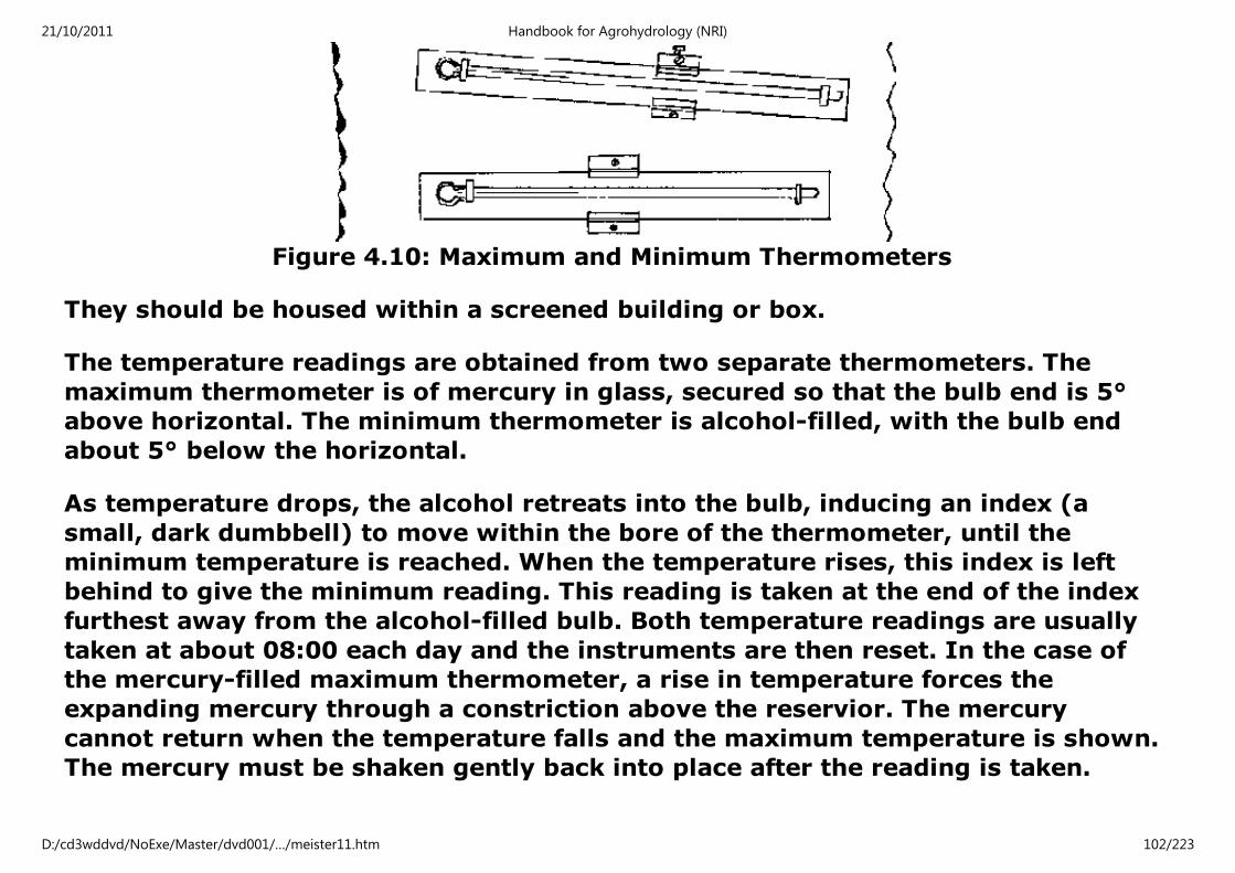
Figure 4.10: Maximum and Minimum Thermometers
They should be housed within a screened building or box.
The temperature readings are obtained from two separate thermometers. The
maximum thermometer is of mercury in glass, secured so that the bulb end is 5°
above horizontal. The minimum thermometer is alcohol-filled, with the bulb end
about 5° below the horizontal.
As temperature drops, the alcohol retreats into the bulb, inducing an index (a
small, dark dumbbell) to move within the bore of the thermometer, until the
minimum temperature is reached. When the temperature rises, this index is left
behind to give the minimum reading. This reading is taken at the end of the index
furthest away from the alcohol-filled bulb. Both temperature readings are usually
taken at about 08:00 each day and the instruments are then reset. In the case of
the mercury-filled maximum thermometer, a rise in temperature forces the
expanding mercury through a constriction above the reservior. The mercury
cannot return when the temperature falls and the maximum temperature is shown.
The mercury must be shaken gently back into place after the reading is taken.
21/10/2011 Handbook for Agrohydrology (NRI)
D:/cd3wddvd/NoExe/Master/dvd001/…/meister11.htm 102/223

4.2.2 Humidity
The moisture status of the air has a strong influence on rates of soil
evapotranspiration (Et) and open water evaporation, both of which are greater
when the humidity of the air is low. Relative humidity values are widely used in
evapotranspiration equations and two main methods are used to measure
humidity:
The first uses thermodynamic principles and measures temperature differences
between wet and dry thermometers ("psychrometers"). They are set together,
with the wet thermometer slightly lower than the dry and are usually housed as
one unit in a secure metal frame. Around the bulb of the wet thermometer is
placed a wick sheath, which trails into a container of clean, distilled water. The
wick should fit tightly; dust, dirt and insects are sometimes a problem and the
wick may need replacement or cleaning each week. The simplest and most
common type of psychrometer (sometimes also called a "hygrometer") is housed
in a screened box. The natural flow of air around the wet bulb thermometer results
in it registering a lower temperature than the dry bulb thermometer. The use of
psychometric tables converts the readings into dew point temperatures and
relative humidity (RH). Hand-held versions are available for spot readings, these
being whirled around on a handle to encourage ventilation; others use the
assistance of electric fans to achieve this effect.
In the second case the instrument uses the hygroscopic properties of a material
(usually human hair) to determine humidity, and is called a "hair hygrometer". A
series of hairs expand and contract according to atmospheric moisture and
oscillate a pen which marks a trace on a chart, moved by a clockwork drum.
21/10/2011 Handbook for Agrohydrology (NRI)
D:/cd3wddvd/NoExe/Master/dvd001/…/meister11.htm 103/223

Adjustments to the instrument can be made by altering the arrangement of linking
levers.
Hygrographs are usually placed on the floor to ensure stability. Shelves used for
such instruments increase the possibility of readings being affected by vibrations
and for this reason the housing fabric should be strong and rigid. The chart can be
annotated with date of chart replacement, station, reader etc. Checks for correct
readings should be made against psychrometer values when the humidity is high
(early morning or during a rainy period) and low (mid afternoon). Hairs that
become dirty should be cleaned with a soft brush, but eventual replacement will
be necessary. Very often this instrument is linked to a temperature sensor that
gives a continuous record on the chart and can be used as a check or back-up to
the maximum and minimum thermometers. In this case the instrument is called a
hygrothermograph. Less costly, non-recording hair hygrometers are also
available.
4.2.3 Wind Speed and Direction
Wind also has an important effect on levels of evaporation and evapotranspiration.
It removes humid surface air layers from above land and water and can physically
damage crops. Anemometers are used to measure wind speed and duration and
thereby windrun, in km day -1. A standard anemometer has three cups mounted at
120° to each other on a vertical axis. The movement of this rotor closes an
electrical contact which measures and records a standard distance of wind
movement. A continuous record of wind speed and direction is also provided.
Wind direction is obtained by the operation of a single-panel vane. Pen and chart
recorders are usual, but electronic recording of these data on data loggers is now
21/10/2011 Handbook for Agrohydrology (NRI)
D:/cd3wddvd/NoExe/Master/dvd001/…/meister11.htm 104/223

common.
A site that is relatively level is to be preferred, with no obstructions within 100 x
the height of the nearest obstacle. The World Meteorological Organisation's
recommended height is 10m for general speeds, but this height imposes the need
for larger and more expensive mast structures. For use in the calculation of Et
values by the widely-used Penman method, 2m is recommended. Fortunately an
estimate of wind speeds for levels other than of the instrument can be obtained by
the formula:
u2 = (ln z2/ln z1) au1 where (4.1)
u2 is the estimate of wind speed
u1 is the known speed at instrument height
z1 and z2 are the heights in cm of the known and estimated wind speeds
a is an exponent between 1 and 0.6 according to ground surface roughness
Empirically this can be stated as Hellmann's formula:
Velocity at height 'h' / Velocity at 10 m = 0.233 + 0.656 log10 (h + 4.75) (4.2)
Hand-held anemometers with digital displays of wind speed are available, but
these do not incorporate a wind direction sensor. Relatively compact, portable
systems that can be quickly assembled at site, can be purchased. It is useful to
21/10/2011 Handbook for Agrohydrology (NRI)
D:/cd3wddvd/NoExe/Master/dvd001/…/meister11.htm 105/223

note that accurate readings of wind speeds less than 5 km per hour are difficult to
achieve.
4.2.4 Solar Radiation
Solar radiation provides energy for evaporation and plant development. Several
methods of calculating Et use solar radiation as a key parameter, often converted
to net radiation, which takes into account the portion of solar radiation that is
reflected back into the atmosphere. Total incoming shortwave radiation is
measured by solarimeters, sometimes called pyranometers, which sense the
intensity of radiation from the sun and sky, that falls in a horizontal plane.
The portion of all radiation that is transformed into other forms of energy is called
"net radiation". Net radiation is measured as the difference between incoming
(downward) and outgoing (upward) radiation of all wavelengths by the net
radiometer. As radiation varies between night and day, counters can be linked to
the radiation measuring device to record these values separately for easy reading.
Electronic pulses may be recorded on a strip chart, but increasingly (especially
with small, automatic meteorological stations) the data are recorded on an
electronic logger and can be downloaded directly in digital form on to a computer,
for viewing and analysis.
Sites should be clear of obstructions, with a view to the horizon that is not
affected by nearby trees or buildings. Under no circumstances should shading
occur and artificial surfaces that can direct radiation to the instrument should be
avoided. The site should be typical of conditions under study, but compromise is
inevitable where conditions of vegetation type and cover, soil reflection, etc. vary
21/10/2011 Handbook for Agrohydrology (NRI)
D:/cd3wddvd/NoExe/Master/dvd001/…/meister11.htm 106/223

from place to place within the local area. Placing the instrument high, perhaps at
3m, increases the field of reception which is useful in areas that are
heterogeneous. Cultivated field situations are more likely to give representative
values that rangeland areas which tend toward heterogeneity. As a guide, an
instrument set at X metres above the ground will receive 90 and 99% of its
upward flux from ground areas with radii 3X and 10X respectively. Figure 4.12(b)
shows a typical net radiometer that would be one component of a small, automatic
weather station.
It is very important to keep the glass or plastic domes clean and undamaged. The
presence of dust is a common problem. A photographer's air brush is very useful
for cleaning, but if not available, soft tissues can be used. Care should be
exercised as the domes are prone to scratching. The instrument should be kept
horizontal at all times. Calibration is important because of deterioration of the
domes and black reception faces and should be carried out every few months.
However, this involves the use of a replacement radiometer to continue the record
and it may only be possible to check the upper and lower sensors during an off-
season period, when a break in the record may not be important. This is best done
at a time of steady radiation, when the faces of the radiometer are inverted for 10-
minute periods. Averages are taken and both faces should give readings within
5% of each other. Alternatively, a second instrument can be kept in good storage
conditions and used only as a standard for the field instrument. As different
ground conditions may be measured by the two adjacent instruments, it is as well
to exchange their positions around to check the first results.
Solarimeters (pyranometers) measure only incoming short-wave radiation and are
sometimes used at meteorological stations. These can be used to calibrate
21/10/2011 Handbook for Agrohydrology (NRI)
D:/cd3wddvd/NoExe/Master/dvd001/…/meister11.htm 107/223

radiometers. They should be shaded from direct solar radiation by placing the
shadow of a black matte disc (about 1m away and held by a thin support) over the
instruments. The response by both sensors should be the same such that Dr/ Cr=
Ds/Cs. As Dr and Ds, the change in response of the radiometer and solarimeter are
measured (in mv) and Cs, the calibration constant of the solarimeter is known, Cr
can be found. This should be done several times.
Sunshine:
Sunshine hours are commonly recorded where the cost and practicability of
maintaining radiation meters are limiting. The widely-used Campbell-Stokes
recorder consists of a glass sphere mounted on a pedestal which concentrates
bright sunlight onto a chart and so burns a trace along it, thus sunlit periods are
recorded. Instruments which are specified by ranges of operation latitude (for
example 0° to 60° N or S) and the correct charts for the N or S hemisphere should
be used.
Electronic meters that measure photosynthetically active radiation (400 - 700 nm)
are also available.
4.2.5 Evaporation
Evaporation Pans:
The measurement of free surface water evaporation depends on air temperature,
wind, humidity and solar radiation. It is a commonly measured index that
integrates these meteorological factors and to some extent, illustrates the
21/10/2011 Handbook for Agrohydrology (NRI)
D:/cd3wddvd/NoExe/Master/dvd001/…/meister11.htm 108/223

behaviour of evaporation from water bodies and evapotranspiration from wet soil,
where the availability of water is not limiting.
The most commonly used instrument, which is an international reference
instrument, is the US Weather Bureau 1.22 m (4 foot diameter) A-pan. This can be
purchased complete, or made from local material such as a suitable gauge,
galvanised steel sheet. Pressed seams should not be allowed to cause buckling.
Welded seams should be treated to prevent rusting The pan should be mounted
horizontally on a wooden platform with tamped soil below, to allow a 13 mm air
space (half an inch). In humid climates the areas around the pan will be grass,
whereas in arid areas, vegetation will come and go according to season. However,
vegetation should not be allowed to grow above the level of the pan. Locations
near areas with artificial surfaces, boggy areas or water surfaces should be
avoided.
The water level in the pan can be measured by an inclined, graduated gauge staff,
but accurate reading in this manner is more difficult than by using a stilling well
and micrometer hook gauge. The level is measured with the hook tip, lowered
below the water and then raised until the tip just pierces the surface. The
mechanism is removed from the stilling well and the reading taken from the
graduated vernier scale. Water levels should be kept at 5 cm below the rim of the
pan (+/- 2.5 cm) and water should be added or removed to maintain this level. A
reading should be taken before and after this has been done. The differences in
daily levels give evaporation, with additions and removals of water and daily
rainfall (measured nearby) being taken into account. Readings are taken at the
same time each day, normally 08:00 hours, though alternatively a WLR could be
used if the cost is not prohibitive.
21/10/2011 Handbook for Agrohydrology (NRI)
D:/cd3wddvd/NoExe/Master/dvd001/…/meister11.htm 109/223
Daily maximum and minimum temperatures of the pan water are often taken by
floating thermometers, kept at least 30 cm from the side. Problems can occur with
birds and animals drinking from the pan. Fences will keep out larger animals, but a
wire screen fixed over the pan itself, may be necessary. This can effect readings by
the suppression of evaporation and in semi-arid climates a correction of 16% is
made to measurements. Algal growth can be prevented by a small addition of
copper sulphate to the water and the pan should be kept clean of debris and
insects. Figure 4.13 shows a hook gauge version of the Type A evaporation pan.
Data may be lost during periods of heavy rainfall and over-topping.
Lysimeters:
Lysimeters most commonly measure evapotranspiration by changes in the weight
of containers filled with soil, to which water is added. Losses by
evapotranspiration are then calculated. Lysimeters can be very large, weighing
several tons, while others used in field locations may only measure water losses
from a few kilogrammes of soil. Crops and vegetation may or may not be grown in
them. Large containers are weighed by permanent pressure transducers, though
the construction of large lysimeters is normally beyond the scope of many
agrohydrological projects and is not practicable under field conditions.
Meteorological services may find it useful to install them.
Evapotranspiration from small lysimeters is measured by their removal and these
instruments are more commonly used for field research. Suitable ones can be
made from PVC water pipe with a diameter of 15 cm and a length of 20 30 cm.
They are filled by attaching a steel cutting edge to the lower edge of the plastic,
and a metal ring to the top. The latter prevents damage when they are hammered
21/10/2011 Handbook for Agrohydrology (NRI)
D:/cd3wddvd/NoExe/Master/dvd001/…/meister11.htm 110/223
into the ground at the required location, when soils are at field capacity and
drainage has ceased. Jacking lysimeters into the ground may be necessary, but the
appropriate equipment must be available.
The lysimeter is removed and the soil is retained by a wire mesh (5 mm is
suitable), which is screwed into the base. They are then replaced into their holes
which have been fitted with tubes, a few millimetres larger in diameter and deeper
than the lysimeters. Lysimeters are removed and weighed every hour or so
throughout the day. Because the cores are isolated from root activity, new cores
should be taken every 2 to 3 days, to account for plant extraction.
There are other problems of representing true conditions with lysimeters: filling
with soil can disturb the profile, edge-effects are great especially with small
models, isolation leads to hydraulic continuity being lost at the sides and affected
at the base. Intermittent, unexpected rainstorms can affect readings.
4.2.6 Soil Temperatures
Soil temperatures have direct effects on the germination and root growth of crops
and natural vegetation, the state of which can greatly affect runoff. Soil
temperatures determine the micro climate of the overlying air and are important
for assessing the growing environment of crops. Soil temperatures are not only
dependent on incoming and outgoing radiation, but also on the thermal properties
of the soil which can change greatly with the addition of water by rain and its
removal by evapotranspiration. Temperatures reach maximum some time after
local noon and minimum after midnight.
21/10/2011 Handbook for Agrohydrology (NRI)
D:/cd3wddvd/NoExe/Master/dvd001/…/meister11.htm 111/223

Continuous records of temperature can be taken with thermocouples
(thermographs) linked to pen and chart or electronic loggers. Thermocouples
should be calibrated with mercury thermometers at least twice a season, at the
beginning and end, and any corrections must be noted. Bent-stem mercury
thermometers for 10 and 20 cm depths and encased mercury types with bulbs in
crystalline wax and suspended in steel tubes for 50 and 100 cm depths, are used
where recording instruments are not available. These depths are recommended by
WMO. Readings are normally taken at 08:00, 14:00 and 20:00 Local Time. Good
contact with the soil is necessary and accidental trampling should be prevented.
4.2.7 Automatic Weather Stations
Research applications may demand the collection of climatic information at sites
in addition to base stations. In such cases the use of automatic weather stations
may be more suitable than an array of individual instruments. Electronic logging is
used to keep records (usually on a multi-channel data logger) and to avoid the
need for frequent visits. The period between visits is determined by the number of
instruments used, the frequency of record and the memory size of the logger.
Different formats for the presentation of data will be used according to
manufacturer.
21/10/2011 Handbook for Agrohydrology (NRI)
D:/cd3wddvd/NoExe/Master/dvd001/…/meister11.htm 112/223

Figure 4.14 Example Meteorological Data sheet
Stations should be enclosed by fences in a suitable position, as discussed in the
sections on individual instruments. Considerable thought should be given to the
possible problems of vandalism and theft because of the cost of automatic
weather stations and the ease with which the array of instruments can be
damaged.
21/10/2011 Handbook for Agrohydrology (NRI)
D:/cd3wddvd/NoExe/Master/dvd001/…/meister11.htm 113/223

Figure 4.15: Typical Weather Station Layout
Figure 4.14 shows an example data sheet for the meteorological variables
discussed above.
Figure 4.15 shows a plan of suitable weather station site, equipped with a basic
list of individually installed instruments. Note that sufficient space is left within
the compound to accommodate instruments that may be installed at a later date.
It is important to select automatic weather stations according to particular project
needs, for example some stations place anemometers below the recommended 10
21/10/2011 Handbook for Agrohydrology (NRI)
D:/cd3wddvd/NoExe/Master/dvd001/…/meister11.htm 114/223

m elevation, and if wind speed and direction are important factors in the research
agenda, this may not be suitable. Automatic weather stations can be very cost
effective when their prices are compared to those of collections of individual
instruments. Generally, the seven following meteorological parameters are
measured:
- rainfall and relative humidity
- air and soil temperature
- wind speed and direction
- solar radiation.
Equipment costs
All costs of locally made equipment are approximate. The costs of raw materials
and especially labour are highly variable from country to country, but a good idea
of cost magnitude can be gained from the figures quoted below. The costs of
manufactured equipment are based on 1993 prices. Shipping, agents' fees and
fluctuations in exchange rate cannot be taken into account.
21/10/2011 Handbook for Agrohydrology (NRI)
D:/cd3wddvd/NoExe/Master/dvd001/…/meister11.htm 115/223
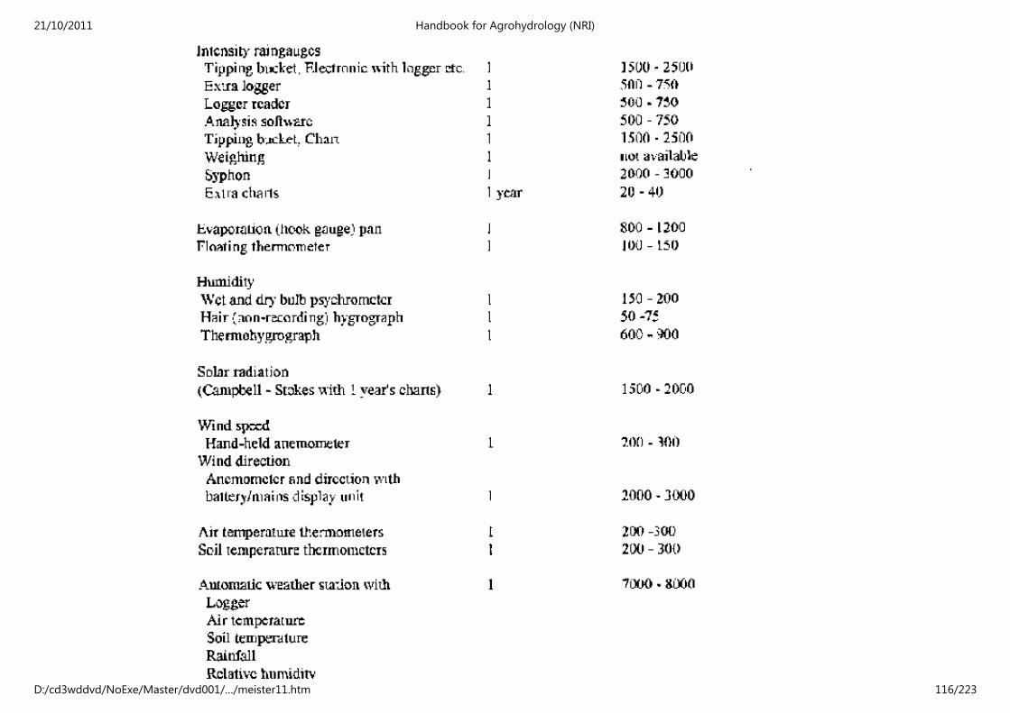
21/10/2011 Handbook for Agrohydrology (NRI)
D:/cd3wddvd/NoExe/Master/dvd001/…/meister11.htm 116/223

Table
Home"" """"> ar.cn.de.en.es.fr.id.it.ph.po.ru.sw
Handbook for Agrohydrology (NRI)
Chapter 5: Soils and soil moisture data
(introduction...)
5.1. Soil classification and soil textures
5.2. Soil moisture
5.3 Infiltration
Equipment costs
Appendix C: Soils and soil moisture
Handbook for Agrohydrology (NRI)
Chapter 5: Soils and soil moisture data
Soil physical, chemical and moisture properties constitute a study in their own
right and it is possible that any agrohydrological or water harvesting project may
have available the services of a soil specialist, but this is not always the case. The
effects of soil physical properties on hydrological behaviour are very important.
21/10/2011 Handbook for Agrohydrology (NRI)
D:/cd3wddvd/NoExe/Master/dvd001/…/meister11.htm 117/223
Four main aspects of soils and their influence on runoff and agriculture are
considered. These are:
1. The physical and textural nature of soils which are influential in
determining runoff.
2. The soil moisture status which can also influence runoff and control
water availability for crops.
3. How to measure soil moisture.
4. The influence of these soil factors on the process of infiltration, the
ability of soils to absorb water.
In many respects soil textures and soil moisture status are closely linked; the
physical characteristics of soils may change with the addition or removal of water,
while the physical characteristics of soils will determine their ability to absorb and
retain rainfall. In terms of the study of soils for agrohydrological purposes and the
quantification of soil characteristics, it is most convenient to study these aspects
separately. Methods of determining infiltration, which is strongly influenced by
texture and moisture status, are also discussed.
5.1. Soil classification and soil textures
5.1.1 Soil Horizons and Their Characteristics
The soil profile, as exposed by the side of a pit is usually divided into 3 horizons
which are frequently further divided into sub-horizons:
21/10/2011 Handbook for Agrohydrology (NRI)
D:/cd3wddvd/NoExe/Master/dvd001/…/meister11.htm 118/223

A horizon constitutes the top soil, where any organic matter is found and within
which cultivation is initiated. B horizon is the subsoil, without organic matter. C
horizon which is composed of weathered rock, usually the parent material.
Soil pits, dug to give an exposure of the soil to the C horizon where possible,
provide a great deal of information which is used in the classification of the soil
types. From the agrohydrological viewpoint however, it is the practical effects on
farming and hydrology of such factors as the effective depth of soil (that is the
depth that can provide a medium for roots) that are important. In most cases the
effective depth is limited by the nature of parent material and the manner in which
it has weathered; climatic influences are often strong. In other cases, gravel bands
may be present and if tightly bound, will restrict the development of crop roots.
Such bands should be noted as the limit of the effective depth. Roots may be
evident in partially weathered parent material but it is unlikely that they
contribute much to the intake of crop water and nutrients. Information on parent
material, erosion, formation history and climate, indicate past periods of
waterlogging and other aspects of the nature of the soil moisture reserve.
Topsoils
Of particular importance is the character of the top 20 cm or so of soil. This is the
soil layer that influences soil surface/rainfall relations by its texture and aeration,
and represents the approximate depth of cultivation. The top soil layer also
determines structural stability, fertility, and the tendency for a soil to cap or
erode. There are obvious limitations to digging large numbers of pits in order to
determine soil characteristics; the job is a long and arduous one and pits must
usually be filled in after examination. The textural definition of surface soils is
21/10/2011 Handbook for Agrohydrology (NRI)
D:/cd3wddvd/NoExe/Master/dvd001/…/meister11.htm 119/223

therefore more commonly assessed by working the soil by hand, when wet. Where
an accurate textural analysis of soils is needed, samples are taken and analysed in
the laboratory (see chapter 3). Table 5.1 below lists the characteristics of soil
textural types when manipulated.
Sandy soils have high rates of infiltration and percent runoff is usually low. They
tend to be infertile, relatively acid and prone to leaching. At the other extreme,
clay textured soils give high percent runoff in general, though cracking vertisol
soils may absorb water until the clay particles swell, the cracks close and runoff
results from later rain. Fine textured soils normally have a higher water holding
capacity than coarse, sandy soils and their chemical mix is more varied and
nutritious for plants.
21/10/2011 Handbook for Agrohydrology (NRI)
D:/cd3wddvd/NoExe/Master/dvd001/…/meister11.htm 120/223

Table 5.1: Soil Textures According to Manipulation When Wet
Soil depths are also important; whatever the inherent water holding capacity of
soils on a unit volume basis, the absolute volume of water available to crops will
be small if soils are shallow. This is an important consideration when the viability
of water harvesting opportunities is being assessed, as it will be a critical factor in
determining how frequently water must be added to the soil moisture reserve.
21/10/2011 Handbook for Agrohydrology (NRI)
D:/cd3wddvd/NoExe/Master/dvd001/…/meister11.htm 121/223
Soil textures are determined precisely and classified most rigorously in the
laboratory as described in chapter 3. The FAO has now adopted the USDA soil
classification triangle which categorises soils into textural types according to the
percentage of silt, sand and clay components, and is shown in Figure 5.1. The
"International" classification (Figure 5.2) is now used in few countries. Relatively
small differences exist between them. Several approaches can be taken to the
selection and collection of soil samples. Spatially, soil textures can be highly
variable, so that when top soil samples are collected to assess the general textural
type of a large area (for instance a whole field), samples are taken at individual
points and combined well before submission for analysis. If the spatial variation of
soil textures is in itself a characteristic under investigation, samples should be
taken systematically on a marked grid basis, with each sample given a point
reference number accordingly. This avoids subjective sampling.
Where microtopographical features are under study, sampling should take place
along defined transects at every one or two metres, according to transect length.
Again, the samples are referenced to the sample points and also to the elevations
above a base level (a levelling survey will be necessary). Wash-ins, ploughing,
crops, vegetation and faunal activity may be recorded. Loose samples (not cores)
are collected and sealed in polythene bags and the depths to which they are taken
are noted. See chapter 3 for details regarding the dispatch of soil samples.
21/10/2011 Handbook for Agrohydrology (NRI)
D:/cd3wddvd/NoExe/Master/dvd001/…/meister11.htm 122/223

Figure 5.1: FAO/USDA Soil Classification Triangle
21/10/2011 Handbook for Agrohydrology (NRI)
D:/cd3wddvd/NoExe/Master/dvd001/…/meister11.htm 123/223

Figure 5.2: International Soil Classification Triangle
Subsoils
Subsoils affect soil water permeability and thereby runoff. In the field,
permeability is usually assessed by the observation of soil physical characteristics
rather than direct or laboratory measurement of hydraulic conductivity. Common
terms used in descriptions are:
21/10/2011 Handbook for Agrohydrology (NRI)
D:/cd3wddvd/NoExe/Master/dvd001/…/meister11.htm 124/223

Compacted: Firm or hard consistency, close packing of particles resulting in a
dense material with reduced pore space.
Cemented: Hard and brittle, soils which do not soften with prolonged moistening.
Deflocculated: Soils in which sodium has entered the exchange complex and
dispersed the colloids. This leads to reductions in pore space, aeration and
permeability. High levels of pH and electrical conductivity are found. Columnar
horizons which are hard and dense may be found.
The colour of soils may give information on aeration and drainage and are
described according to the standard Munsell notation. Colours may vary between
and within horizons, for example:
Drainage: Reds Well drained
Yellows, Greys Poorly drained
Organic Matter: Browns & Blacks High in organic matter
Leaching: Paler Moreleached
Darker Less leached and higher mineral fertility
Wet soil colours are usually darker and there may be the presence or absence of
mottles. The colours on Munsell charts that provide the standard reference
(described in detail below), are arranged to give the three variables used to define
all colours and are recorded in a standard order:
Hue: The dominant spectral colour (increase in redness or yellowness).
21/10/2011 Handbook for Agrohydrology (NRI)
D:/cd3wddvd/NoExe/Master/dvd001/…/meister11.htm 125/223
Value: The lightness of colour and total amount of light reflected.
Chroma: The purity or strength of colour (increases with a reduction of greyness)
On each card the colours are of a constant hue. The colours increase in lightness
vertically and in equally visible steps. The colours increase in chrome to the right
and become greyer to the left. In the field, a 1 cm fragment is selected from the
sub soil, untainted by organic matter. After deciding whether it is predominantly
yellow or red, a colour chart is selected and the sample compared through the
most appropriate hole in the chart. Intermediate matches are not uncommon.
Check that the hue is correct. Avoid sweat on the colour charts (not always easy).
Mottles, very pale and very dark colours indicate reduced permeability or
groundwater near the surface. Rust-coloured mottles along root channels suggest
periodic waterlogging, as does an abrupt change from reddish to greyish
colouration. Grey mottles in an otherwise reddish weathered rock zone indicate a
seasonal water table.
Bulk Density
Soil texture is largely responsible for the bulk density of soils, that is the weight
per unit volume, most commonly expressed as g cm-3. Imperial units of lb ft-3
may be seen. Bulk densities are found by comparing the oven dry weight of
samples and their volume. Samples are taken from soil pits using standard soil
sampling cores, driven into the exposed face below the top soil when the soil is
neither very wet nor completely dry. The sample must not be disturbed, so as to
maintain its original volume. The sample should be oven dried at 105 °C to 110 °C
21/10/2011 Handbook for Agrohydrology (NRI)
D:/cd3wddvd/NoExe/Master/dvd001/…/meister11.htm 126/223

and weighed to the nearest 0.1 gram.
The bulk density (sometimes called the "specific weight") dry weight of sample/
volume of sample The bulk density in g cm-3 can be converted to lb ft-3 by
multiplying by the factor 62.4.
Soils with high bulk densities have a paucity of pore space, impede root
penetration, make cultivation difficult and promote runoff.
5.1.2 Pedological Classification
The pedological classification of soils, although basically created with agriculture
in mind, is described only briefly here. It is relatively complex and includes an
extremely wide range of soil types. Many of the terms and names derive from the
Russian language. Soil surveys and maps use the orthodoxy of pedological
classification, but in developing countries soil mapping is usually at an early stage
or restricted to localities of special interest. Map scales are commonly 1: 250,000
to 1:1,000,000 and cannot be expected to depict the variability of soil types with
accuracy.
The pedological classification of soils is broken into two main groups: Higher and
Lower categories. Of the higher categories, the nature of Zonal soils depends
greatly on the prevailing climate at the time of formation. Intrazonal soils not only
are influenced by climate, but also localised conditions, for instance poor
drainage, and therefore cross the boundaries of zones. Azonal soils such as
lithosols (rocky) and regosols (dry sandy) are not zonal.
In arid and semi-arid regions, regosols, lithosols and lateritic soils (which are red
21/10/2011 Handbook for Agrohydrology (NRI)
D:/cd3wddvd/NoExe/Master/dvd001/…/meister11.htm 127/223
and have a high iron oxide and aluminium hydroxide content) are commonly
found. Variation in soil types is wide and intrazonal soils may commonly occur due
to changes in local conditions of geology and drainage. Calcareous bands may be
common at depth.
Glei are indicative of impeded drainage and a rising and falling of the water table.
These mottled colourations may be red, yellow or brown when the water table is
low, or grey or blue when it is high, resulting from the oxidisation or non-
oxidisation of iron and manganese.
Higher Categories
There are three main orders of soils (Zonal, Intrazonal and Azonal) which are sub-
divided into Suborders and Great Soil Groups:
Zonal Soils Suborder Great Soil Groups
1. Cold zone Tundra,
2. Light coloured arid zone Desert, Red desert, Sierozem,
Brown/Reddish-brown soils
3. Dark coloured soils of semiarid sub humid
and humid grasslands
Chestnut, Reddish-chestnut, Chernozem,
Prairie, Reddish prairie soils
4. Forest grassland transition Degraded Chernozem and Noncalcic
brown soils
5. Light coloured timbered regionsGrey wooded or grey podzolic soils
21/10/2011 Handbook for Agrohydrology (NRI)
D:/cd3wddvd/NoExe/Master/dvd001/…/meister11.htm 128/223

Grey wooded or grey podzolic soils
6. Laterite soils of forested warm temperate
and tropical regions
Reddish brown and Yellow brown lateritic
and Laterite soils
Intrazonal soils
1. Halomorphic
(saline and alkali)
Saline, Soloth, Solonetz soils soils of
imperfectly drained arid regions
2. Hydromorphic soils
of marshes
Humic-glei, Low humic glei, Bog, and swamps Groundwater packed
soils
3. Calcimorphic soils Brown forest soils
Azonal soils Lithosols, Regosols,
Alluvial soils
Further classification is beyond the scope of this book. The Unified System,
developed in the USA, is concerned with the engineering aspects of soil
classification, rather than agriculture.
Lower Orders
The Great soil groups are subdivided into Soil Series and then Types. Series are
soils developed from the same parent material and soils within a series have the
same profile characteristics except for the texture of the surface layer. Types are
determined by the texture of the A horizon. Soil Phases are determined by
deviation from the norm, for example a stony phase.
5.2. Soil moisture
21/10/2011 Handbook for Agrohydrology (NRI)
D:/cd3wddvd/NoExe/Master/dvd001/…/meister11.htm 129/223

The soil moisture content of a soil is of primary importance. Soil moisture is
expressed either in percent by weight (Pw) or volume (Pv) . The relations are:
Pw = (Ww - Wd/Wd) × 100 and (5.1)
Pv = ( Vw / Vs) × 100 (5.2)
respectively, where the subscripts w and d are wet and dry samples and Vs is the
volume of the sample.
Percent weight of water is the most common (gravimetric) determination and is
found by using samples obtained from the field. Samples can be taken with
shovels, augers or soil sampling cores. Samples are best transported for
immediate drying in electric ovens at 105° C in sealed cans to prevent moisture
loss; this temperature removes all moisture, without driving off other volatile
matter.
Balances should weigh to the nearest 0.1 g and samples should each weigh at
least 100 am. With a typical weight of moisture of the sample being 20 g, the
accuracy of measurement will thus be approximately 0.5 %. Several samples will
be needed and areas used continually for sampling may suffer. Soil heterogeneity
can be a problem, though as discussed previously, the manner in which samples
are collected determines the extent of this difficulty.
The usefulness of volumetric determinations of soil moisture content lies in their
easy conversion to surface units. This conversion allows comparison with rainfall
and irrigation applications, although percent volume determinations are not
usually obtained by direct sampling. The volume of water from soils could be
21/10/2011 Handbook for Agrohydrology (NRI)
D:/cd3wddvd/NoExe/Master/dvd001/…/meister11.htm 130/223

estimated by determining the weight of moisture and converting to volume
assuming a specific gravity of 1.0 for water, though the volume of soil is difficult
to measure. Field determination of soil moisture on a volume basis is normally
found using a neutron probe. This is method discussed later.
5.2.1 Soil Moisture Potential
The soil moisture potential (SMP) represents the thermodynamic energy status of
a soil and is conventionally expressed in units of bars (1 bar - 106 dynes cm-2).
Two particularly important specific points of soil moisture conditions are field
capacity and wilting point. Field capacity is the condition whereby moisture is
retained after the gravity drainage of a saturated soil is complete and the soil
moisture tension is equal to one third of an atmosphere. Wilting point is the
condition beyond which plants can no longer extract water and is taken to be a
tension of 15 atmospheres. Soil moisture between these two points is regarded as
that available to plants.
Total SMP is composed of three components:
Potential energy due to the force of gravity, osmotic potential and capillary
potential. The latter is by far the most important and is assumed to be more or
less equal to the total soil moisture potential. Equipment is available to measure
this variable in the field.
Since many occasions arise when either the soil moisture content (SMC) or
capillary potential can be measured, a relation between them is desirable; this
could be used to describe the SMP. Unfortunately, a unique relation does not exist
21/10/2011 Handbook for Agrohydrology (NRI)
D:/cd3wddvd/NoExe/Master/dvd001/…/meister11.htm 131/223

for most soils and the moisture content depends not only on capillary potential,
but also on previous soil moisture history. The effect of this is that two main soil
moisture relations exist (see Figure 5.3), one for the dewatering of the soil (the
soil moisture retention curve) and another for rewetting. These soil
moisture/suction conditions are called the "hysteresis loop" and it is often
represented in graphical form.
In many situations it is suitable to refer only to the dewatering branch of the
hysteresis loop since this has the most profound effect on plant growth. It is
obtained and applied under drying conditions. In very many cases these relations
are unique to the soil, though some generalisation is permitted and related to field
(and sometimes project) conditions. In some soils the two branches of the
hysteresis loop may be relatively close and it can be assumed that they are the
same for all practical purposes, though this is not usually the case. Table 5.2 gives
typical soil moisture values for various soil types.
21/10/2011 Handbook for Agrohydrology (NRI)
D:/cd3wddvd/NoExe/Master/dvd001/…/meister11.htm 132/223

Figure 5.3: Typical Soil Hysteresis Loop
21/10/2011 Handbook for Agrohydrology (NRI)
D:/cd3wddvd/NoExe/Master/dvd001/…/meister11.htm 133/223

Table 5.2: Typical Moisture Values for Various Soil Types
Table 5.3 below gives a field guide for judging how much of the available water
has been removed from different soils.
Equipment for the measurement of SMP, with the exception of the neutron probe,
usually consists of a material that is placed in the soil to reach equilibrium with
the soil moisture and as such measures capillary potential, not SMC. Care should
be exercised in the use of this equipment since the hysteresis behaviour makes the
step from capillary potential to SMC problematic.
The soil retention curve is sometimes called the soil characteristic and is found by
laboratory analysis. Tensiometers can be used in the field, but the limit of the
suction pressure that they exert is very low (about 0.8 bar), whereas the use of a
pressure plate apparatus in the laboratory gives a much wider range and water
content can be found by weighing the sample at each stage of dewatering. The soil
moisture retention curve can then be plotted (Soil moisture in % versus suction in
bars), using the data points.
With regard to sampling, spatial variability in soils is the norm and the
21/10/2011 Handbook for Agrohydrology (NRI)
D:/cd3wddvd/NoExe/Master/dvd001/…/meister11.htm 134/223

representative nature of sites that are selected will be limited. Microtopography,
runon, runoff, the lateral flow water within horizons and land use are some of the
factors that affect soil moisture variability. A number of sites will be needed
within a "homogeneous " area and the extent of study will depend on the aims and
resources of a particular project. Knowledge of the degree of soil variability is in
itself a useful tool in assessing the place of water harvesting and agrohydrological
research in the agricultural agenda. A survey at the outset of a project, that is as
comprehensive as resources permit, will usually be extremely rewarding. Where
possible, work that has been undertaken previously by soil surveys and land use
planning organisations should be consulted.
21/10/2011 Handbook for Agrohydrology (NRI)
D:/cd3wddvd/NoExe/Master/dvd001/…/meister11.htm 135/223

Table 5.3: Field Guide for Judging Available Soil Moisture
5.2.2 In situ Methods of Soil Moisture Measurement
21/10/2011 Handbook for Agrohydrology (NRI)
D:/cd3wddvd/NoExe/Master/dvd001/…/meister11.htm 136/223

a. Tensiometers
Tensiometers are used to measure capillary potential, the sensing elements are
usually porous ceramic membranes or pots. Usually a water and mercury
manometer is attached to these membranes to measure potentials, though dial
type gauges can be used. The manometers are housed to prevent weather damage
(especially sunlight and high temperature) and a set may have perhaps six or ten
sensors, each placed at different depths, to cover the possible range of plant
rooting.
Various manufactures of tensiometers are available and the instruction manual
should be followed carefully. The tensiometer must be saturated with water to
work properly and is installed after the membrane has been boiled to remove
gases, filled with boiled water and transported to the field wrapped in wet rags or
in a container of water. To protect against damage the clear plastic tubing, sealed
into the porous pot and placed in a plastic pipe of suitable internal diameter
(usually about 2 cm) and length, is lowered into a pre-prepared hole. To ensure
good hydraulic contact with the soil, some of the excavated soil from the hole is
mixed with water and poured in as a slurry, to act as a seating. Careful back-filling
of the hole with the soil is necessary to avoid a depression at the surface. Time
must elapse before the slurry dries out, which if below the rooting zone, may take
several weeks. Figure 5. 4 shows the installation of mercury manometer
tensiometers
21/10/2011 Handbook for Agrohydrology (NRI)
D:/cd3wddvd/NoExe/Master/dvd001/…/meister11.htm 137/223

Figure 5.4: Mercury Manometer Tensiometers
The tubing is charged using boiled (degassed) water with a large syringe to
prevent air bubbles. As the porous pot is in contact with aerated soil however, it is
likely that bubbles in the tubing may be a recurrent problem. Modest housing fixed
to metal poles with a hinged door for access and painted white to reflect heat is
adequate. Installations at every 20 cm depth are suitable.
Points to note:
- Tensiometers are used for monitoring moist soils because of their narrow
range of sensitivity.
- Boiled water is always used for filling and flushing.
- Theoretically, tensiometers cannot measure negative pressures greater
than one atmosphere, but in practice their limit is less than this, about 0.8
of one atmosphere, greater tensions will encourage air to enter the system.
21/10/2011 Handbook for Agrohydrology (NRI)
D:/cd3wddvd/NoExe/Master/dvd001/…/meister11.htm 138/223
- In very arid conditions, appreciable volumes of water may be passed
through the membrane and may affect soil conditions.
- Tensiometers are subject to thermal variations and it is best if readings
can be made during early morning, several time a week, depending on
conditions.
- Adequate regard to routine monitoring and rainfall conditions must be
given for remote field sites. Flushing with boiled water to remove air
bubbles (which make the manometer operate incorrectly) must be part of
the routine.
- Vacuum gauges may be used instead of mercury manometers. They are
more robust, but may be less sensitive.
b. Electrical Resistance Method
This method of measurement involves the use of blocks of porous material, usually
gypsum (calcium sulphate), though sometimes units of fibreglass or nylon
construction are preferred. The block material will tend toward a potential
equilibrium with the surrounding medium. They are placed in good contact with
the soil and the electrical resistance of the block gives an estimate of soil moisture
content. Gypsum blocks are best buffered against saline soils, although they are
less sensitive to changes at high moisture contents and generally deteriorate more
quickly than the fibreglass and nylon alternatives. The blocks come provided with
electrical connections in the form of wires or coaxial cables.
Before installation they should be saturated and a resistance reading taken for
21/10/2011 Handbook for Agrohydrology (NRI)
D:/cd3wddvd/NoExe/Master/dvd001/…/meister11.htm 139/223
reference. They are installed in the same manner as tensiometers, but a shallow
horizontal trench should be dug with a slope away from the blocks, in which the
wires can be laid, to avoid water being directed downwards them and resulting in
incorrect readings. Though of simple construction and relatively cheap, the main
disadvantage of these devices is their relative insensitivity to changes in the high
soil moisture content range.
Points to note:
- They can be used in much drier soils than tensiometers.
- Gypsum blocks operate best at tensions 1 to 15 atmospheres (drier soils).
- They will last for 2 or 3 seasons.
- Nylon and fibreglass operate best at tensions of less than 2 atmospheres,
but they are more expensive and are sensitive to salts.
- The materials are relatively cheap, but difficulties include unobserved
deterioration while underground, attack by chemicals with consequent
errors and a possible drift of the calibration curve.
- More than one unit can be used per installation hole, but great care must
be exercised during emplacement.
- The blocks must be calibrated in the laboratory.
Calibration
21/10/2011 Handbook for Agrohydrology (NRI)
D:/cd3wddvd/NoExe/Master/dvd001/…/meister11.htm 140/223

Two methods of laboratory calibration are in general use. The first is to place the
resistance block in a small container surrounded by soil that is initially saturated
and to allow the soil to dry out gradually, reaching various levels of moisture
content, each of which is determined by weighing the whole system. At each level,
a reading of electrical resistance is also taken. The second method is preferable,
but depends upon the availability of a pressure plate or pressure membrane
apparatus. The resistance block is placed in a pad of soil in the pressure apparatus
which is best equipped with the facility of electrical connection through its wall,
thus allowing continuous monitoring of the block. The soil is initially saturated
and when equilibrium is reached (water no longer flowing out) a resistance
measurement is taken. The block is brought progressively, in steps, to various
levels of desorption and the measurements of electrical resistance are repeated.
Where accurate and comprehensive field soil moisture measurements are to be
made, the blocks should be calibrated for both wetting and drying, to overcome
the problems of hysteresis. Soils of different textural characteristics must each be
calibrated separately.
c. Neutron Probe Method of Soil Moisture Determination
Neutron probes emit fast neutrons from a small radioactive source (typically 50 -
100 millicurie mCi ). The neutrons are slowed when they encounter hydrogen
atoms in the soil and these slow neutrons are registered by a boron trifluoride
detector integral to the instrument. Unaffected fast neutrons are not detected. The
detection of slow neutrons is amplified and counted by a rate-scaler. As water is
the main source of hydrogen atoms in the soil (though organic matter, boron and
chlorine will also slow the neutrons), the number of slow neutrons reaching the
detector is a function of soil moisture content. The neutron probe has a limited
21/10/2011 Handbook for Agrohydrology (NRI)
D:/cd3wddvd/NoExe/Master/dvd001/…/meister11.htm 141/223

diameter of detection of about 20 - 30 cm.
The neutron probe consists of the main body which houses the cable, clamps,
rate-scaler and handles. The source and detector are lowered on the cable into an
aluminium access tube in the ground (aluminium being more or less transparent
to neutrons). Readings are taken at required depths. The base of the probe body
usually has a shield to prevent inadvertent irradiation when the cable is wound in.
Figure 5.5 below shows the main components of a neutron probe.
Access tubes
The observation holes that are used for neutron probes are made permanent by
casing them with a thin walled material, usually aluminium. Aluminium is almost
transparent to neutrons, is durable and can be purchased in varying diameters.
The latter is a significant practical point as it is important to select diameters of
tubes that give the practical minimum air gap between the probe and the access
tube wall, while allowing unimpeded access to the source and detector. This air
gap will affect the instrument's count-rate.
Commonly, a single piece of tube is used, with the upper end protruding above the
soil surface. This not only aids location, but in many cases is used as a seat for the
probe. It is essential to match the outside diameter of the access tube with the
inset of the neutron probe or the diameter of the tubes will have to be modified at
a later date. Example (but not exclusive) diameters are: tube outside 44.45 mm,
thickness 2 mm, internal diameter 40.45 mm probe diameter 38.00 mm. The
surface exposed portion of the access tube should be kept to an acceptable
minimum but as
21/10/2011 Handbook for Agrohydrology (NRI)
D:/cd3wddvd/NoExe/Master/dvd001/…/meister11.htm 142/223

it is usually used as seat for the probe body, this portion should be adequate for
the purpose. To prevent dirt and water from entering, a rubber bung is fitted.
Covering this with a soft drinks can gives extra protection. Usually, condensation
is not a problem, butt where it is, small sacks of desiccant should be hung in the
tube.
Figure 5.5: Main Components of a Typical Neutron Probe
Installation
The installation of access tubes can be one of the most difficult and time-
21/10/2011 Handbook for Agrohydrology (NRI)
D:/cd3wddvd/NoExe/Master/dvd001/…/meister11.htm 143/223

consuming aspects of neutron probe field work. Hard, dry soils, gravel, concreted
layers and high bulk densities make observation hole excavation problematic,
despite the development of mechanical installation systems. In fortunate
circumstances, hand excavation by auger is possible. The main criterion of
effectiveness of installation is the snugness of fit of the access tube within the
hole. This depends not only on the method of installation, but also on the type and
wetness of the soil. All sites around the access tube should be protected from
trampling and soil compaction by the use of wooden frames or palettes, upon
which the operator can stand. Vegetation around the tube should not be disturbed
if it constitutes part of the actual environment.
Installation by hand:
Continually hand-auger from within the tube in depth stages of 20 cm, remove the
material, then push the tube down. This should ensure a good fit. The tube will
shear off a little soil material as it is placed, but the undersized hole gives
snugness of fit. Some workers excavate an oversized hole and after the tube is
installed, back-fill with the soil material. Whichever method is used, tropical and
sub-tropical soils are often too hard for hand boring. Ingenuity of the individual
worker is often required to solve the problems of installation, which may be quite
different from site to site.
Mechanical installation:
One example of a field-tested mechanical installation device is given below, it was
developed from a geological sampler, capable of excavating to 25 m. It is
illustrated in Figure 5.6.
21/10/2011 Handbook for Agrohydrology (NRI)
D:/cd3wddvd/NoExe/Master/dvd001/…/meister11.htm 144/223

An initial hole is made to about 0.5 m using a guide tube and sledge hammer. Then
solid steel string sections, joined by threaded joints, push down a 0.6 m cutting
tube head under the force of a hydraulic jack-hammer. Depending on the soil, the
excavation may proceed in stages of 20 -50 cm. It may be necessary for the
cutting tube to be locally manufactured, to the same diameter as the access tubes.
The cutting tube is retrieved by the use of a ball clamp and hydraulic ram which
operate from the hammer compressor, pouered by an 11 hp petrol motor. The soil
is removed from the cutting head by screw augers, though this can be a difficult
task as the soil is highly compacted. Breakages tend to occur in the string joints
and the cutting tubes need to be sharpened frequently. They often how after
prolonged use.
Location
The precise site location of neutron probe access tubes should be considered
carefully. The radius of detection is small and combined with soil spatial
variability, can lead to unrepresentative sampling. Moreover, the variability of
surface water infiltration, sometimes due to soil type, but more usually due to
local runoff distribution, can be very great. Soil moisture in low areas generally
penetrates further and a water table may be present in such locations. It is
advisable not to plumb the water table, to avoid submersion of the probe. If field
crops are under investigation, access tubes to 2 m, possibly 3 m, will be adequate.
Much deeper access tubes will be necessary to study deep drainage, but there is
no value in placing access tubes to great depth unless this is warranted; it merely
increases the cost and time involved in installation, monitoring and analysis, to
little purpose. Where the interest is to monitor the variability of soil moisture due
to pronounced topographic features, access tubes should be located on or within
21/10/2011 Handbook for Agrohydrology (NRI)
D:/cd3wddvd/NoExe/Master/dvd001/…/meister11.htm 145/223

the features. Where a field-wide representation is required, access tubes should
be located on a predetermined grid, so that random sampling operates. The depth
of access tubes should also be considered carefully where there is topographic
variability.
Figure 5.6: Acces Tube Instalation Equipment
Neutron probe access tubes are relatively cheap to install and the temptation to
over-monitor must be resisted; large quantities of raw data will be produced
which must all be quality checked and analysed. Moreover, sites require constant
21/10/2011 Handbook for Agrohydrology (NRI)
D:/cd3wddvd/NoExe/Master/dvd001/…/meister11.htm 146/223

monitoring on a routine basis and additional site visits after important rainfall
events will be necessary. It is important not to over-stretch resources of time,
transport and manpower. Access tubes that have been installed but which cannot
be monitored, or backlogs of data that cannot be processed not only create a
sense of frustration, but are a waste of time, money and effort that could be used
elsewhere.
Operation
Standard counts are used as a routine method of checking the performance of
neutron probe equipment. A variety of faults that cause a drift in the count-rate
under identical conditions may be found, and standard counts should be
performed before each time the probe is used and, preferably, after. An important
use of standard counts is calibration between instruments, thus allowing their
interchangeable use, a great advantage when planning any monitoring schedule.
There are two types of standard count:
Water barrel counts are taken with the probe seated on an access tube section
which can be conveniently mounted in a 200 litre oil drum. The drum should be
thoroughly cleaned, water-proofed and filled with clean water. A three-barred
support welded to the top edge of the barrel and holding the tube section in a
vertical position is suitable. A length of tube, perhaps 25 cm, should extend out of
the water. Ten counts of approximately one minute each are adequate.
Shield counts are taken with the probe retracted into the shield of the unit and
with the unit standing on its carrying case. This method of checking the
instrument is especially useful at field sites where water barrel facilities cannot be
21/10/2011 Handbook for Agrohydrology (NRI)
D:/cd3wddvd/NoExe/Master/dvd001/…/meister11.htm 147/223

maintained, though during this calibration the same prevailing conditions are not
so easy to replicate. Ten shorter duration counts, perhaps 15 seconds each, are
sufficient.
The equipment will vary according to manufacturer, but certain aspects of
operation are common. Care should be taken in packing and in transit. The battery
supplies will need constant recharging at the design rates and cannot be expected
to last more than a year or so; a good supply of spare batteries is essential. The
probe cable is susceptible to damage with use as it carries the weight of the probe
and detector unit and is continually being reeled in and out. Spares should always
be available. Jamming of the source and detector in the access tube may occur and
exacerbate the problem of cable damage.
Modern probes usually have depth indicators integrated with the rate-scalers. On
the whole, rate-scalers that require a manual record of count-rates are best to
purchase, although some types with integral memories are available as
alternatives. The latter are perhaps are less robust and more susceptible to
damage. If they malfunction data may be lost and the equipment is rendered
unusable for some time. Neutron probes, though generally very reliable, are
complex instruments and local repairs are often impossible. It is best to have one
complete unit available as a spare.
Protection to the operator must be given by emphasising that while the
radioactive source used in the instrument is very small, any exposure to radiation
constitutes a needless risk. Radiation badges that are pinned to the clothing of the
operator should be purchased, to monitor any exposure to radiation. In developing
countries, it is likely that these will have to be sent overseas to be evaluated. It is
21/10/2011 Handbook for Agrohydrology (NRI)
D:/cd3wddvd/NoExe/Master/dvd001/…/meister11.htm 148/223
also well worth remembering that the transport of radioactive material, in many
countries, is restricted by certain laws. Although these may not pose problems for
routine movement from site to site, they may require special customs clearance
procedures to be effected. Before purchase is complete, the appropriate local
authority should be consulted so that paths may be cleared and frustrating delays
in obtaining the equipment can be avoided.
Calibration
Neutron probe count-rates need to be calibrated, as both individual instruments
and soils behave differently. For example, high bulk densities give higher count-
rates for the same soil moisture content. Neutron probes are supplied with
calibration curves as a guide, but these are constructed in the laboratory and are
seldom appropriate for the soils under investigation. Calibration curves developed
by other researchers may be of interest, but generally the same problems apply.
Calibration must always be undertaken if soils are suspected as being sufficiently
individual to necessitate this. Different manufactures of instrument will greatly
affect count-rate/soil moisture relations.
Field Calibration
In essence, calibration consists of taking count-rates at specified depths in the
soil profile; for example at 10, 40, 70, etc. cm depths. Soil samples are then taken
at these depths for soil moisture and bulk density analysis. It is important to note
here, that compared to deep readings shallow readings may not be accurate nor
consistent, because of the loss of fast neutrons through the soil surface. As a
consequence count-rates tend to be lower and separate calibration curves should
21/10/2011 Handbook for Agrohydrology (NRI)
D:/cd3wddvd/NoExe/Master/dvd001/…/meister11.htm 149/223

be constructed for the top 30 cm or so of the soil profile. Calibration is a relatively
time-consuming business and due the nature of the method, will destroy the
further usefulness of the access tube location. Proceed as follows:
- An access tube is installed, or an existing tube is used.
- Two wooden pegs are sunk 1 m either side of the tube and made level
using a board and level. The soil surface is scraped level and the height
above the board noted.
- The soil moisture profile is monitored at 10, 40, 70 cm below the soil
surface, first with the probe at the height that readings are usually taken
above the soil surface with the instrument sitting on the access tube
(where applicable), then repeated after the tube has been tapped level with
the soil surface. Several readings at each depth should be averaged, to
minimise random errors.
- Duplicate cores taken close to, but on opposite sides of, the tube are
removed with their mid point at 10 cm depth. At the same time a duplicate
pair of cores are taken in the same way, at right angles to the first pair.
- Excavate a 1 m diameter soil pit accurately to 20 cm below the original
surface and using the level board make it so for 35 cm radius around the
tube.
- The tube is then sawn off, tapped down or replaced with a shorter one
(the former has the advantage of less soil disturbance), then the 40 cm
depth is re-monitored at +5 and 0 cm above the soil surface.
21/10/2011 Handbook for Agrohydrology (NRI)
D:/cd3wddvd/NoExe/Master/dvd001/…/meister11.htm 150/223
- Ten cm of soil is removed and the original 40 cm depth re-monitored.
- Core samples are taken once more.
- A new soil surface is located at SO cm below the original and the last
three steps repeated for the original 70 cm depth.
- The soil samples should be analysed for volumetric water content and
bulk density. The analysis of particle size distribution links calibration to
soil textural type.
- Deeper horizons can be calibrated if it is felt that a need exists.
Each calibration, carried out as above, yields 3 points for the 10 cm calibration and
2 points for the 20 and 30+ cm calibrations. It is probably best to limit the number
of such calibrations to one per day, to ensure good working practice, though two
are possible and should enable soil moisture relations at all research sites to be
established.
Calibration is necessary at the wet, intermediate and dry parts of the calibration
curve, where seasonal variations in rainfall lead to extreme differences in soil
moisture content. This can be undertaken after continual rain (or artificial
wetting), after a period of drying and at the end of the dry season. Figure 5.7
shows an example of the field calibration of neutron probe data.
21/10/2011 Handbook for Agrohydrology (NRI)
D:/cd3wddvd/NoExe/Master/dvd001/…/meister11.htm 151/223

Figure 5.7: Field Calibration of Neutron Probe Data
Cross Calibration of Different Manufactures of Neutron Probe
It is quite possible that different makes of neutron probe may be used by the same
project or associated projects. In this case it is preferable to compare water barrel
and access tube counts rather than to repeat the procedures of field calibration for
both types of instrument. Cross calibration may be regarded as essential and is
undertaken as follows:
21/10/2011 Handbook for Agrohydrology (NRI)
D:/cd3wddvd/NoExe/Master/dvd001/…/meister11.htm 152/223

Count rates are taken in the water barrel access tube at 2 cm intervals from above
the water level to 25 cm below its surface, then at 5 cm intervals to 35 cm.
Averages of duplicate counts are taken for each instrument. In field access tubes,
first one probe is used then the other, and this is repeated for average readings.
Usual probing depths, for example every 10 cm, are used. Where instruments
show accumulated count-rate totals, these must be converted to count-rate.
Figure 5.8 show the 30+ cm calibration curve for some semi-arid soils, with Count
-Rate/ Water Barrel Rate (the Count-Rate Ratio, R/RW) versus Moisture Volume
Fraction. Figure 5.9 shows a graph comparing the countrates of one make of
neutron probe with another.
Figure 5.8: 30+ cm Calibration Curve for 10 Semi-arid Sandy Loam Soils
21/10/2011 Handbook for Agrohydrology (NRI)
D:/cd3wddvd/NoExe/Master/dvd001/…/meister11.htm 153/223

Figure 5.9: Comparison of Count-Rate Ratios for Two Manufactures of Neutron
Probe
d. Time Domain Reflectometry (TDR)
TDR measures soil moisture content by utilising large differences in the dielectric
properties of soils, water and air. Methods exploiting these soil/water properties
have been in development for several decades, but it is only very recently that
TDR has become a convenient, practical tool for soil moisture investigation.
21/10/2011 Handbook for Agrohydrology (NRI)
D:/cd3wddvd/NoExe/Master/dvd001/…/meister11.htm 154/223
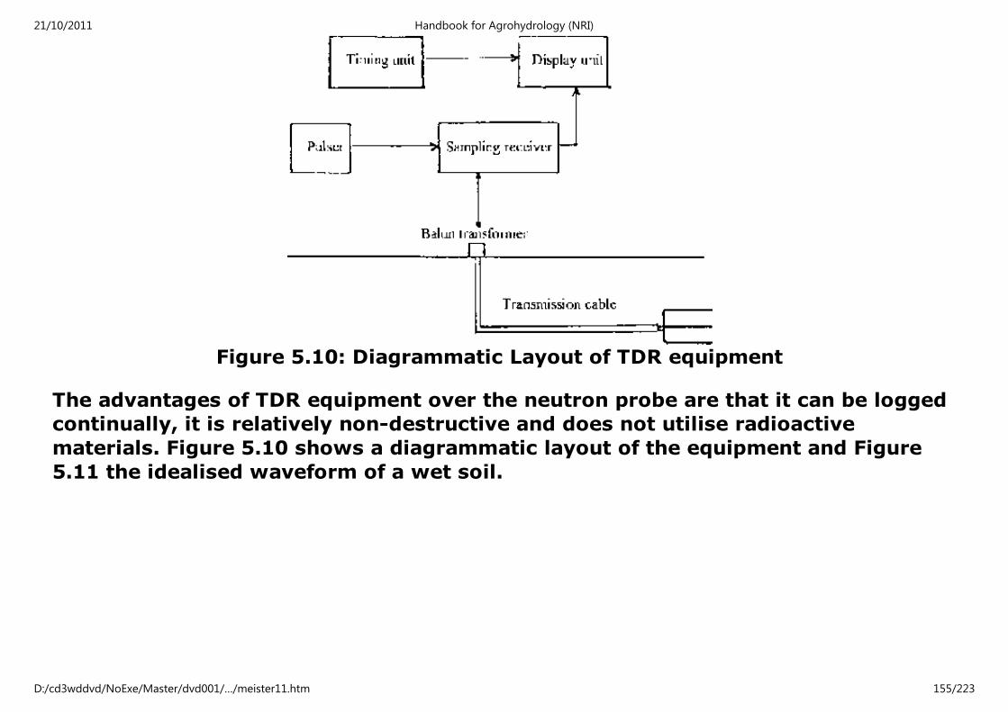
Figure 5.10: Diagrammatic Layout of TDR equipment
The advantages of TDR equipment over the neutron probe are that it can be logged
continually, it is relatively non-destructive and does not utilise radioactive
materials. Figure 5.10 shows a diagrammatic layout of the equipment and Figure
5.11 the idealised waveform of a wet soil.
21/10/2011 Handbook for Agrohydrology (NRI)
D:/cd3wddvd/NoExe/Master/dvd001/…/meister11.htm 155/223

Figure 5.11: Idealised TDR Waveform of a Wet Soil
Principles of Operation
A pulse generator creates a fast rise-time voltage pulse (about 10-10 seconds)
which passes through a transmission line to a balun transformer designed to
achieve maximum transmission into the soil. The pulse then passes to the
waveguide (a pronged "fork" or "probe") in the soil. An impedance mix-match
causes part of the pulse to be reflected back to the instrument, while part is
propagated to the end of the waveguide, from where it is then reflected back to
instrument. The analysis of the waveform (change in voltage) of the pulse that is
21/10/2011 Handbook for Agrohydrology (NRI)
D:/cd3wddvd/NoExe/Master/dvd001/…/meister11.htm 156/223

reflected from the ends of waveguide is the key to measurement. The
interpretation of the waveform is somewhat subjective.
Point C shows the rise-time of the pulse (usually 10-10 to 30-10 seconds), the
point A represents the location of the balun transformer, the distance between C
and A depends upon the length of the transmission cable. Point B is the reflection
from the end of the waveguide. The travel time 't' is the time in nanoseconds for
the pulse to pass from A to B and back. Pulse attenuation, the loss of magnitude of
the signal, increases with moisture content. The calculation of the apparent
dielectric constant, Ka, (approximately 80 for water, 1 for air and 2-4 for soil
minerals) is made by:
Ka = (t c/L)2 where (5.3)
t = travel time
c= speed of light (29.979 cm ns-1) and
L= length off the waveguides in cm.
TDR instruments can be "multiplexed", utilising a variety of waveguide lengths set
to log continuously on a series of channels at a given time interval and controlled
by a small computer. However, it may take half an hour to obtain a set of
measurements and any rainfall during the logging cycle could give confusing
results if the logging cycle were short. Continuous monitoring opens many
opportunities for the detailed examination of moisture changes, especially at
shallow depths, but generates a large amount of data.
Much development has concentrated on waveguide ("probe") form. There are two
21/10/2011 Handbook for Agrohydrology (NRI)
D:/cd3wddvd/NoExe/Master/dvd001/…/meister11.htm 157/223

main types:
Unbalanced waveguides have three prongs, the inner prong, for example, carrying
a positive charge and acting as the centre of a coaxial cable, the two outer prongs
carrying half a negative charge and acting as the shield.
Balanced waveguides have only one outer prong and the lack of shielding is
compensated for by a balun transformer acting as a shield. They are regarded as
more sensitive and less destructive, but are more expensive and can hinder
interpretation by inducing interference on the waveform.
Practical considerations
The sampling volume of the instrument is very small (radius of sampling within
about 1 mm of the waveguide surface) and may be greatly effected by the near-
surface environment, though research into these effects is as yet inconclusive.
Waveguides are (usually) placed horizontally at various depths, avoiding the
penetration of soil layers with different characteristics. This often necessitates the
excavation of a trench behind the locations of the waveguides.
The length of the waveguide prongs is an important consideration. Usually they
are between 0.05m and 1.0m long. The suitability of length is determined by the
attenuation characteristics of the soils under examination. Long prongs offer a
greater volume of sampling, but are more difficult to install and are not suitable
for highly conductive soils. Spacing between prongs of the waveguide is usually
no more than ten times their diameter, with an upper limit of 5 cm. Wider spacing
leads to difficulties in the interpretation of the (greatly attenuated) waveform.
21/10/2011 Handbook for Agrohydrology (NRI)
D:/cd3wddvd/NoExe/Master/dvd001/…/meister11.htm 158/223

Increasing the transmission cable length decreases resolution and a maximum of
30m is recommended.
The effects of soil mineralogical composition on TDR is not fully understood.
Research has indicated that heavy clay soils may give anomalous results and clay
content; bound water and bulk density have been shown to influence calibration.
The dielectric constant of a soil is temperature dependent and therefore diurnal
variations may be significant, especially near the soil surface. The influence of
organic material is not yet fully understood, though increasing organic content
tends to reduce the calibration slope of Ka versus water content. Increasing the
bulk density of soils of a given water content decreases the dielectric constant of
such soils, and the installation of the waveguides should disturb the soil as little
as possible. The reduction of air gaps due to installation may be achieved by
wetting the soil before insertion, though the characteristics of soils will determine
the effectiveness of the installation. TDR is unsuitable for use in stony soils, and in
soils that swell and shrink. Waveguides should not become the focus for cracking
and enhanced percolation, nor be sited cross distinct soil boundaries. Soils high in
iron and titanium (and possibly aluminium) minerals have enhanced dielectric
constants. A guide to operational difficulties in various soil types is given below.
Vertisols: Vertical installation should not be undertaken. They may have a low dry
bulk density due to cracking. Organic content may be high; electrical conductivity
may effect attenuation.
Entisols: Relatively unstructured soils with little organic matter.
Aridisols: Conductivity may be affected by salts and high temperatures close to the
21/10/2011 Handbook for Agrohydrology (NRI)
D:/cd3wddvd/NoExe/Master/dvd001/…/meister11.htm 159/223

soil surface.
Mollisols: Grassland soils, often with high organic contents in the upper horizons.
Alfisols: No obvious problems.
Ultisols: High content of iron and/or aluminium may exaggerate moisture
readings.
Oxisols: Low bulk densities may reduce the slopes of calibration. Temperature
effects may be seen and possible influence of oxides which increase conductivity.
Spodosols: Sharp density changes down the horizon. A high organic matter
content in the A horizon may lead to the underestimation of soil moisture content.
Histisols: High in organic matter and will need separate calibration. Bulk densities
tend to be low.
Calibration
Calibration is undertaken for values of Ka versus volumetric water content and
may be done in the laboratory of field.
Laboratory calibration:
Research in the past has concentrated on the water content of substitute materials
rather than soil, for example vermiculite, glass beads and washed sand. More
recently soils have been used and indicate separate calibration curves for organic
21/10/2011 Handbook for Agrohydrology (NRI)
D:/cd3wddvd/NoExe/Master/dvd001/…/meister11.htm 160/223

and mineral soils. However, as for the neutron probe, laboratory calibrations do
not accurately represent the spatial variability of such factors as texture, bulk
density and organic content.
Field Calibration:
Field calibration may involve the measurement of soil moisture by lysimetery,
neutron probes and gravimetric methods, though sampling and oven drying
gravimetric methods are standard. Sampling may be undertaken in a manner
similar to that described above, for neutron pobes. At water contents of greater
than 20%, laboratory calibrations were seen to overestimate moisture content.
Differences between neutron probe and TDR measurements have been found to be
large (10 - 20%) and may reflect the different sampling volumes of the two
instruments. These results indicate that the use of TDR should be carefully
examined and TDR may not be suitable for water balance studies, though its more
precise and accurate measurements can be effectively used in rooting zones and
areas of marked changes in water content over small distances.
Waveform Interpretation
Interpretation determines the value of Ka that is derived from the waveform. An
example of a Ka calculation is given below, with the use of Figure 5.12.
21/10/2011 Handbook for Agrohydrology (NRI)
D:/cd3wddvd/NoExe/Master/dvd001/…/meister11.htm 161/223

Figure 5.12: Hypothetical Waveform
From equation 5.3, Ka = (6 × 29.979/20)2 = 80.89 (the value of Ka is
dimensionless)
Figures 5.13 (a), and 5.13 (b) show the idealised waveforms of air, water.
Figure 5.14 shows how the waveform changes with increasing and soil moisture
content.
21/10/2011 Handbook for Agrohydrology (NRI)
D:/cd3wddvd/NoExe/Master/dvd001/…/meister11.htm 162/223

Figure 5.13 (a): Waveform, Air
Figure 5.13 (b): Waveform, Water
21/10/2011 Handbook for Agrohydrology (NRI)
D:/cd3wddvd/NoExe/Master/dvd001/…/meister11.htm 163/223

Figure 5.14: Waveform, Different Soil Moisture Contents
Below are example waveforms for different soil conditions that may be
encountered. Figures 5.15 (a) shows the waveforms of a waveguide installed
vertically through a wetting front and (b), a dry zone over a wet zone.
Soils with increasing percentages of iron oxides display a waveform of decreasing
amplitude and increasing travel time. Relatively dry, clay mineral soils frequently
exhibit a large amount of background noise which makes interpretation difficult,
while wet clays often exhibit large pulse attenuations, probably due to high pore
water electrolytic concentrations.
21/10/2011 Handbook for Agrohydrology (NRI)
D:/cd3wddvd/NoExe/Master/dvd001/…/meister11.htm 164/223

Figure 5.15 (a)
Figure 5.15 (b)
Figure 16 shows the effect of increasing salinity. The travel time is not changed,
but the magnitude of the pulse decreases as the salinity, and conductivity, of the
soil increase.
21/10/2011 Handbook for Agrohydrology (NRI)
D:/cd3wddvd/NoExe/Master/dvd001/…/meister11.htm 165/223

Figure 5.16: Waveform, Increasing Salinity
e. Capacitance Probe
Capacitance probes, like TDR, have only recently become practical field
instruments for measuring soil moisture. They also measure the dielectric
constants of soils, like TDR, but are relatively low cost. They are usually utilise an
access tube, but recent designs will allow direct insertion into the soil and
readings are usually taken from a hand-held meter. It is necessary to calibrate
these probes for individual soils.
5.3 Infiltration
Infiltration is the process whereby water on the soil surface percolates
downwards. Infiltration rates represent the speed at which this percolation occurs
and are expressed in mm in-l. The maximum rate for any given soil condition is
21/10/2011 Handbook for Agrohydrology (NRI)
D:/cd3wddvd/NoExe/Master/dvd001/…/meister11.htm 166/223

termed the "infiltration capacity". The controls on infiltration rates are many: soil
texture, cavities and impermeable layers, vegetation cover, air spaces, soil
wetness and topography all may be influential. Land use and cultivation can also
be extremely important as they affect the quantity of suspended material in
surface water which in turn influences rates of infiltration, because the suspended
material blocks pore spaces and increases runoff. Measured rates of infiltration
lump the effects of all these influences together.
Runoff is the proportion of rainfall that does not infiltrate, at least immediately,
but infiltration rates vary greatly with time, especially during rainstorms when the
soil becomes progressively wetter and as rainfall intensities vary. Thus the supply
rate of water to the soil surface and the rate at which it infiltrates are never
constant. Despite the fact that infiltration rates represent a gross generalisation of
soil/water behaviour, they are often important components of hydrological and
runoff models.
Extensive field trials have shown that infiltration rates decrease with time, in the
general form:
I = (aTn + b) where (5.4)
I = infiltration rate
a, b and n are constants and
T= Time elapsed
Thus infiltration rates are exponential. As the rate of infiltration decreases it
approaches, and sometimes achieves, a terminal value. For clay soils, the value of
21/10/2011 Handbook for Agrohydrology (NRI)
D:/cd3wddvd/NoExe/Master/dvd001/…/meister11.htm 167/223

'b' in equation 5.4 may be almost zero, while for sandy soils it will be much
greater; soil texture plays an important part in the determination of infiltration
rates. Infiltration rates are used not only to estimate the likelihood of runoff, but
are also quoted as a general soil characteristic, but it should be noted that the
infiltration rates of soils are notoriously spatially variable, even over distances of
a few metres.
Figure 5.17: Variation of Infiltration Rates Over Small Areas
Variability is important because it can be associated with microtopography in
21/10/2011 Handbook for Agrohydrology (NRI)
D:/cd3wddvd/NoExe/Master/dvd001/…/meister11.htm 168/223

fields and cultivation practices which alter the location of topsoils. For example
Figure 5.17 shows the variation of infiltration rates of 20 tests undertaken over an
area only 15 m square, on an apparently uniform soil. Variation will affect the
redistribution of runoff at the local scale and will be influential in determining the
soil moisture that is available to plants. Important differences between rates on
cultivated and uncultivated land are likely to be seen.
Figure 5.18 shows example infiltration curves for different soil textwal types:
sandy, loamy and clay soils.
Figure 5.18: Example Infiltration Curves for Sandy, Loamy and Clay Soils
Three methods of measuring infiltration are discussed below.
21/10/2011 Handbook for Agrohydrology (NRI)
D:/cd3wddvd/NoExe/Master/dvd001/…/meister11.htm 169/223

5.3.1. Equipment and Methods of Measurement
a. Double Ring Infiltrometers
Double ring infiltrometers consist of two concentrically placed rings, both filled
with water. The rate of infiltration into the ground within the inner ring is
measured, while the water in the outer ring provides a buffer to ensure the direct
downward movement of water below the inner ring.
Infiltrometers can be purchased, but as they are simple to manufacture to specific
requirements, this may be preferred. They can be made by using metal water pipe
cut to a suitable length and given a bevelled, sharpened edge at one end. Example
dimensions are: length 30 cm, diameter 60 cm, the smaller ring should be of the
same length, but half the diameter, also sharpened. The two different sized rings
are inserted into the ground, the depth of insertion will depend on the hardness of
the soil. A more or less constant head of water is maintained at a measured and
marked level (10 cm is suitable) above the ground surface. Water is poured into
both rings until it reaches this level and then another 1 litre of water is added.
When the water in the inner ring falls to the marked level another litre is poured
in, to compensate for infiltration. If infiltration is slow, only 0.5 litre need be
added; the water in the outer ring is also kept to the level and generally it will
take one or two hours to reach a constant (terminal) rate of infiltration. Figure
5.19 shows the installation of the double ring infiltrometer.
21/10/2011 Handbook for Agrohydrology (NRI)
D:/cd3wddvd/NoExe/Master/dvd001/…/meister11.htm 170/223

Figure 5.19: Double ring Infiltrometer.
The accuracy of the data collected from infiltrometers may be affected by the
insertion of the rings, which can alter the physical characteristics of the soil. Soils
with macropores, burrows etc. may show extreme rates of infiltration and prove
to be unsuitable for study by this method. Crusted soils can be prepared by cutting
the crust with a razor blade and inserting the rings through the cuts. The gap
between the ring and soil may be sealed with gypsum paste or hydraulic cement.
The major difficulty with data that are obtained by the double ring method
however, is that they do not represent infiltration under rainfall/runoff conditions:
rainfall impact may increase or reduce infiltration at the soil surface; rain storm
intensities vary greatly and the standing heads of water used by these
infiltrometers are not usually representative of real conditions. Runoff flows away
and is not impounded. The spatial variability of infiltration capacities is common
and results may be relevant only to very small areas. It is important to note,
however, that data from double-ring infiltrometers are widely used and it may be
essential to collect this information if comparisons between a range of sites and
soils are to be made. The dates' main value is as a reference for comparison rather
than the provision of absolute, true infiltration rates, though these may be of
21/10/2011 Handbook for Agrohydrology (NRI)
D:/cd3wddvd/NoExe/Master/dvd001/…/meister11.htm 171/223

direct application to irrigation practice. To overcome the unrealistic results that
double ring infiltrometers often provide, sprinkle infiltrometers have been
developed. An approximate replication of natural rainfall can be obtained by the
use of sprayers and sprinklers. Sprinklers can be complex systems that simulate
duration, rate, drop size etc., but even the smallest versions of these instruments
are not really portable and often require large volumes of water to operate.
Knapsack sprayers are low cost alternatives that can be easily transported and
when used carefully, provide relatively good data.
b. Knapsack Spray Infiltrometer
Spray infiltration tests using knapsack sprayers improve upon the results from
ring infiltrometers by minimising the effect of a standing head of water and by
applying the water as a spray. Further emulation of the rainfall/ infiltration
process is not attempted. Although this method is only a rudimentary attempt to
simulate rainfall it does provide an improved technique which is portable, easily
replicated and inexpensive. Typically, a quadrat is sprayed at a designated rate
which is reduced upon the evidence of standing surface water. Details of the
method are as follows:
An area 1 m square is marked and within it a 50 cm × 50 cm × 5 cm deep wooden
quadrat is placed centrally, pushed 2 -3 cm into the ground. The central quadrat is
divided into quarters. Wind shields should be provided around the site if
necessary. The sprayer is best fitted with a fan nozzle to provide a wide, even
spray. The 1 m² quadrat is sprayed with an even application every 30 seconds. The
period of pumping to prime the sprayer and the duration of application are
regulated (for example pumping and application for 5 and 10 seconds
21/10/2011 Handbook for Agrohydrology (NRI)
D:/cd3wddvd/NoExe/Master/dvd001/…/meister11.htm 172/223

respectively) to give a similar intensity spray each time. When water is seen
standing on two or more of the central quarters, the next spray is omitted. This
may be continued for an hour or more, or until a recognisable uniformity of
application indicates stability of the infiltration rate. The amount of water
delivered is quantified by repeating the spray test procedure into a measuring
vessel before and after the test. The total volume of water that can be applied
during the test will depend upon the nozzle aperture, but depths of 40 mm can
easily be achieved. Variations on this method may be designed to account for local
conditions.
This method, though not representing true rainfall conditions, is relatively simple
and easy to replicate and the data obtained discriminate clearly between soils of
different texture. The rates also resemble those that might be expected under
rainfall conditions. Figure 5.20 shows a vertical view of equipment layout used in
running tests with a knapsack sprayer.
Figure 5.20: Knapsack Infiltration Test Equipment (Vertical View)
21/10/2011 Handbook for Agrohydrology (NRI)
D:/cd3wddvd/NoExe/Master/dvd001/…/meister11.htm 173/223

Testing may be undertaken on cropped, range or fallow land. The simulation of
ploughing effects can be achieved by digging the soil over; this may be necessary
in regions that have distinct dry and wet seasons. In these areas testing is most
suitably undertaken during the dry season, when the influence of rainfall and high
levels of antecedent soil moisture are not evident. It is likely that fields will not be
cultivated at this time.
c. Sprinkler infiltrometers (Rainfall Simulators)
Unlike double-ring infiltrometers, sprinklers are not limited to the study of
infiltration rates. They are often used to investigate such influences on the
rainfal/runoff process as soils, slopes and tillage practices and may be used to
measure rates of soil erosion. It is convenient however, to discuss this type of
equipment here. Sprinklers attempt to simulate the process of rainfall, while
allowing a control over the amount, intensity and drop size of applications in a
manner that is not possible with natural rainfall. Though they represent
rainfal/runoff conditions more realistically than ring infiltrometers and portable
knapsack sprayers, sprinkle infiltrometers also have limitations. An important
question to ask when considering sprinkler design is which of the main rainfall
characteristics should be simulated most closely: for example drop-size or
terminal velocity? Variations in intensity or uniform applications? Difficulties exist
even in measuring the characteristics of the natural rainfall that is being
simulated.
Design
Sprinkler design can be esoteric, and "production models" are not common. Most
21/10/2011 Handbook for Agrohydrology (NRI)
D:/cd3wddvd/NoExe/Master/dvd001/…/meister11.htm 174/223

sprinklers cannot be considered at all portable, they are too large and even small
sprinklers may need compressors, pumps or a mains water supply to operate.
Large, boom type sprinklers are usually confined to agricultural research stations
where there is a plentiful supply of water and where it is preferable to maintain
tight control over the soil, slope, cover and tillage variables under investigation.
As runoff and soil loss are related to rainfall kinetic energy per unit area, this is a
useful parameter by which to make comparisons of sprinklers. In general two
types of rainfall simulations are adopted.
The first type are those using nozzles which most easily reproduce a drop size
distribution akin to natural rainfall, but which have complex intensity reducing
systems.
The second use drop-formers and are simpler in construction, but the drops do not
reach terminal velocities until falling 5 m or more.
It is far beyond the scope of this book to describe the many individual types of
sprinklers that have been developed, often for particular research purposes, and
which are not easily nor commercially available. A comparative list of such
equipment is given in Part 1 of monograph no. 9 of the American Society of
Agronomy and Soil Science Society of America (1986). Most sprinklers of the
"portable" kind apply water to relatively small areas, usually about 1 m². The
problem of spatial variability of soil characteristics is therefore often as great with
these devices as it is with ring infiltrometers and knapsack sprayers, and the
extrapolation of results beyond the locality of application needs careful
consideration.
21/10/2011 Handbook for Agrohydrology (NRI)
D:/cd3wddvd/NoExe/Master/dvd001/…/meister11.htm 175/223

The Type F infiltrometer has been used in the USA on larger plots of approximately
2 m × 4 m in size and is not regarded as portable. the type FA operates over a
smaller area. The manner of operation to obtain infiltration data is recommended
as follows:
- First, several calibration runs are undertaken with the test area covered
by a waterproof sheet, to measure the simulated rainfall application rate.
- A test run is then started with the sheet removed and continued until the
rate of runoff becomes constant (as does the rate of infiltration).
- The analytical run is started when application ceases and runoff stops,
but before any recovery of the infiltration capacity has occurred. The rate
of infiltration is therefore constant throughout the run. Runoff is measured.
Any difference between the application minus infiltration and runoff is due
to depression storage and detention storage.
- The effects of these on the runoff process may be investigated for various
land conditions, if required.
The relation between runoff and infiltration data is discussed further in chapter 8,
Data Analysis
Manufacture
The most important components of sprinklers are the nozzles that control the
characteristics of the water that is applied to simulate rainfall. The testing of
suitable nozzles on an individual basis was undertaken by the Ministry of
21/10/2011 Handbook for Agrohydrology (NRI)
D:/cd3wddvd/NoExe/Master/dvd001/…/meister11.htm 176/223

Agriculture, Harare, Zimbabwe as part of research into the SLEMSA soil erosion
model (see chapter 3), over 1 m² areas. Of the various nozzles tested, several
performed well and details are given in the Ministry's Research Bulletin no 25
(1980). The construction details of a mobile sprinkler taken from this bulletin are
given Appendix C.
Equipment costs
All costs of locally made equipment are approximate. The costs of raw materials
and especially labour are highly variable from country to country, but a good idea
of cost magnitude can be gained from the figures quoted below. The costs of
manufactured equipment are based on 1993 prices. Shipping, agents' fees and
fluctuations in exchange rate cannot be taken into account.
21/10/2011 Handbook for Agrohydrology (NRI)
D:/cd3wddvd/NoExe/Master/dvd001/…/meister11.htm 177/223

21/10/2011 Handbook for Agrohydrology (NRI)
D:/cd3wddvd/NoExe/Master/dvd001/…/meister11.htm 178/223
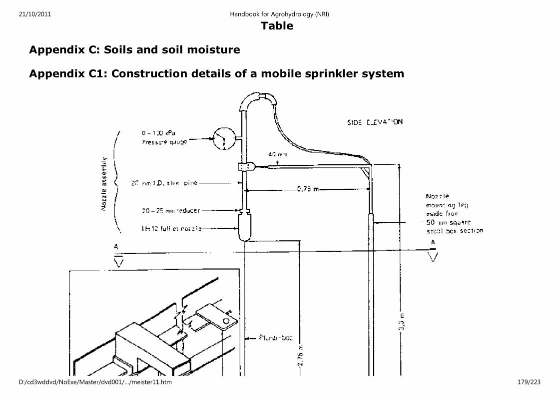
Table
Appendix C: Soils and soil moisture
Appendix C1: Construction details of a mobile sprinkler system
21/10/2011 Handbook for Agrohydrology (NRI)
D:/cd3wddvd/NoExe/Master/dvd001/…/meister11.htm 179/223

Figure
21/10/2011 Handbook for Agrohydrology (NRI)
D:/cd3wddvd/NoExe/Master/dvd001/…/meister11.htm 180/223

21/10/2011 Handbook for Agrohydrology (NRI)
D:/cd3wddvd/NoExe/Master/dvd001/…/meister11.htm 181/223

Plan on A - A
Windshield frame
21/10/2011 Handbook for Agrohydrology (NRI)
D:/cd3wddvd/NoExe/Master/dvd001/…/meister11.htm 182/223

Plan on driving dolly
21/10/2011 Handbook for Agrohydrology (NRI)
D:/cd3wddvd/NoExe/Master/dvd001/…/meister11.htm 183/223

Fig. 1: IH12 nozzle assembly details
21/10/2011 Handbook for Agrohydrology (NRI)
D:/cd3wddvd/NoExe/Master/dvd001/…/meister11.htm 184/223

21/10/2011 Handbook for Agrohydrology (NRI)
D:/cd3wddvd/NoExe/Master/dvd001/…/meister11.htm 185/223

Fig. 2: Size distributions for IH12 nozzle
Home"" """"> ar.cn.de.en.es.fr.id.it.ph.po.ru.sw
Handbook for Agrohydrology (NRI)
Chapter 6: Catchment characteristics
(introduction...)
6.1 Natural vegetation
6.2 Interception
6.3 Catchment size, slope and topography
6.4 Field orientation
6.5 Antecedent soil moisture conditions
6.6 Other catchment influences
Equipment costs
21/10/2011 Handbook for Agrohydrology (NRI)
D:/cd3wddvd/NoExe/Master/dvd001/…/meister11.htm 186/223

Handbook for Agrohydrology (NRI)
Chapter 6: Catchment characteristics
Catchment characteristics interact with variable patterns of rainfall and determine
the character and size of runoff volumes and peak flows. This is true for both
natural catchments where human activity is absent or unimportant and runoff
plots upon which tillage or other agricultural treatments are being tested.
Generally, there is a hierarchy of influence imposed by different characteristics,
but this hierarchy is often difficult to sort out and understand. For example, where
a catchment has high slopes and lime vegetation, slope will play a major role in
determining the runoff regime. This regime would tend to exhibit high runoff
proportions; rapidly increasing flows to high peaks and equally rapid falls. Were
this catchment to be of a more linear form and were its vegetation cover to
increase, then peak flows would be smaller but more prolonged and total runoff
volumes would probably be less. Were the slope lower, runoff would probably be
less.
In the case of catchments with low slopes, the effects of vegetation cover and
microtopographic features often exert a stronger influence over runoff than the
overall land slope. Local slopes are often relatively high and they may direct runoff
either into basins where it can infiltrate or to channels by which it can easily leave
the catchment. Heavy textured soils tend to give a higher proportion of runoff. Soil
textures are related to slope as well as to parent material, and the climatic regime
under which the soil formed will often have been a determining factor of the soil
textural type. Where human interventions have been imposed the natural
21/10/2011 Handbook for Agrohydrology (NRI)
D:/cd3wddvd/NoExe/Master/dvd001/…/meister11.htm 187/223
conditions of a catchment may have been altered radically; grazing, tree-felling
and clearance are obvious examples. Agricultural techniques; ploughing, bunds
and microcatchments are introduced to reduce runoff and usually they do, but the
removal of natural vegetation and badly managed systems can have the opposite
effect. Below, the main catchment characteristics and their influence on runoff are
discussed.
6.1 Natural vegetation
Natural vegetation can be very important in determining runoff amounts; in many
instances it is the most important influence of all, after rainfall. Areas bare of
vegetation can lose more than 40% of seasonal rainfall through runoff and for
intense, individual storms the loss can be much greater. Areas with dense grass
cover and tree canopy cover can retain as much as 99% of the rainfall that reaches
the ground. Vegetation reduces the energy of raindrops making them less erosive
and intercepts rainfall which is then re-evaporated. Thus natural vegetation works
against the occurrence of runoff in several ways. The same can be said of crops,
but most crops provide only temporary cover and their densities, especially at
ground level, rarely attain that of natural vegetation. Examples of increased runoff,
soil erosion and subsequent land degradation due to the removal of natural
vegetation, are common throughout the world and the literature. Consider the
data presented below in Table 6.1, which compares runoff from different
rangeland catchments of the same size catchments, but with various densities of
vegetation cover.
21/10/2011 Handbook for Agrohydrology (NRI)
D:/cd3wddvd/NoExe/Master/dvd001/…/meister11.htm 188/223
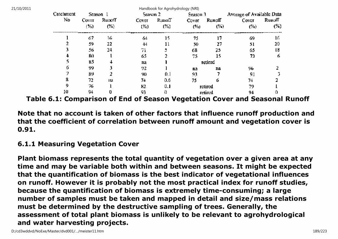
Table 6.1: Comparison of End of Season Vegetation Cover and Seasonal Runoff
Note that no account is taken of other factors that influence runoff production and
that the coefficient of correlation between runoff amount and vegetation cover is
0.91.
6.1.1 Measuring Vegetation Cover
Plant biomass represents the total quantity of vegetation over a given area at any
time and may be variable both within and between seasons. It might be expected
that the quantification of biomass is the best indicator of vegetational influences
on runoff. However it is probably not the most practical index for runoff studies,
because the quantification of biomass is extremely time-consuming; a large
number of samples must be taken and mapped in detail and size/mass relations
must be determined by the destructive sampling of trees. Generally, the
assessment of total plant biomass is unlikely to be relevant to agrohydrological
and water harvesting projects.
21/10/2011 Handbook for Agrohydrology (NRI)
D:/cd3wddvd/NoExe/Master/dvd001/…/meister11.htm 189/223

The form of vegetation; leave-shape, density, branching pattern, etc., is highly
variable between species and groups of plants. Although these differences are
implicit within the classification of plant species, their effect on rainfall/runoff
relations are very difficult to quantify. Research into commonly-occurring trees
(and crops) has been undertaken, but the results of this work is understandably
limited in its applications. Moreover, biomass and vegetation cover are usually
very closely correlated and the use of vegetation cover as a proxy for biomass in
runoff analysis, is a legitimate substitution.
Figure 6.1 show example correlations between biomass and vegetation cover and
vegetation cover and runoff.
21/10/2011 Handbook for Agrohydrology (NRI)
D:/cd3wddvd/NoExe/Master/dvd001/…/meister11.htm 190/223

Figure 6.1: Biomass and Vegetation Cover
21/10/2011 Handbook for Agrohydrology (NRI)
D:/cd3wddvd/NoExe/Master/dvd001/…/meister11.htm 191/223

Figure 6.1: Vegetation cover and Runoff
In contrast to biomass measurement, there are rapid methods of quantifying the
areal extent of total vegetation cover and even though effects due to vegetation
type are not always accounted for, this index makes a good indicator of the
influence that vegetation can have on runoff.
Vegetation cover assessments may be undertaken on a frequent basis to study its
effect on runoff, almost storm by storm. Alternatively, assessments may made
only a few times each season, to understand its role in the production of runoff
over longer periods. The latter case is most common, because the variation in
21/10/2011 Handbook for Agrohydrology (NRI)
D:/cd3wddvd/NoExe/Master/dvd001/…/meister11.htm 192/223

influence of vegetation cover is not dramatic in the short term, except where
wholesale removal is involved. Vegetation cover is not closely correlated to other
factors that influence runoff (except perhaps seasonal changes in rainfall and
temperature), but may considerably alter the soil moisture status by
evapotranspiration. The relative independence of vegetation from other variables
makes it a suitable factor for use in regression analysis. On the other hand
because it does vary with time, unlike factors such as slope, soil type and
catchment size, vegetation cover can provide an extensive range of data points for
individual catchments. It lends itself well to and is often used in, runoff modelling.
In general it has been recognised that the amount of vegetation cover present is a
more influential factor than the type of cover. The pattern of spatial distribution of
vegetation cover may also be very important.
For agrohydrological purposes, there are two conventional methods of cover
measurement, though the collection of aerial photography and satellite remote
sensing data are also discussed below.
a. Quadrats.
A quadrat is a defined area. For field purposes, quadrats are usually permanent
sampling areas retained throughout the season, within which the extent of
vegetation cover is assessed. Prior to the field visit that will install them, a
suitable number of quadrats is decided upon and these are placed on a site map
using a fixed grid pattern. The quadrats are laid out in this predetermined, regular
manner to overcome subjective bias and attain a random sampling of the area. No
strict percentage sampling is required, though the more quadrats, generally the
better. Ten 2m × 2m quadrats to sample 1 ha (10,000 m²) would be adequate. The
21/10/2011 Handbook for Agrohydrology (NRI)
D:/cd3wddvd/NoExe/Master/dvd001/…/meister11.htm 193/223

quadrats are then subdivided into four sectors to facilitate accurate assessment.
The quadrats can be made easily by using steel rods driven into the ground with
perimeters defined by nylon rope or string. Each quarter of the quadrat is
individually assessed by eye for percent total ground cover of live and dead
vegetation. The overall estimate of cover is made as an average of all sectors and
all quadrats. In cases of natural vegetation, any trees are included in the
assessment. Assessments should be made as frequently as is feasible throughout
the season, though the rate of growth will largely determine the need for
inspection The estimates are to some extent subjective and it is a good idea to
compare those made by different field staff, under the same conditions of cover.
This method is suitable for small areas and can be completed quickly, but projects
that need to quantify cover accurately on large plots and small catchments can
utilise a rapid method that is detailed below.
b. Wheel Point Method
This method is based on the simple equipment shown in Figure 6.2.
A bicycle handlebar is fitted with an extended fork assembly. The extension is
made long enough to allow the passage between them of strong, sturdy spokes.
The spokes, made of 5 - 10 mm diameter mild steel, are welded to a supporting
plate which in turn is fixed to the axle. The forks can be any convenient length, but
it is advantageous that when the observed, marked fork completes a revolution, it
travels an easily recorded horizontal distance, for example 1.0 or 1.5 m. Versions
with longer or shorter spokes can be made, according to whether the areas to be
covered are small or large, to maintain a sufficient number of data points per unit
21/10/2011 Handbook for Agrohydrology (NRI)
D:/cd3wddvd/NoExe/Master/dvd001/…/meister11.htm 194/223
area of catchment.
As an example, consider a plot 100 × 40 m in extent. A tape measure is stretched
across one of the longer sides of the plot, 5m from the end. The apparatus is held
with the marked spoke at the start of the tape and then walked along using the
tape as a direction indicator.
If the marked spoke hits a bare area on touching the ground, this is called out. If it
touches a vegetated area on the ground this (and if required the type and species
of plant) is called out. A second person notes the call. The tape is then moved on
10 m and the process is repeated, until the whole plot has been covered, the last
transect being 5 m from the other end of the plot.
This procedure gives approximately 600-700 data points for each hectare that is
surveyed and takes about one hour. Less frequent sampling by using more-widely
spaced transects is permissible in areas where the vegetation cover is relatively
uniform. This method is also easily adapted for larger catchments and can be used
in difficult and wooded terrain, with practice.
21/10/2011 Handbook for Agrohydrology (NRI)
D:/cd3wddvd/NoExe/Master/dvd001/…/meister11.htm 195/223

Figure 6.2: Wheel Point Apparatus
c. Aerial Photography
Aerial photographs and, more recently, satellite imagery can play an important
role in the assessment of many aspects of agrohydrology, vegetation cover being
one of them. Clearly, this method is inappropriate for small runoff plots, but for
natural catchments it can be very useful. Large areas can be viewed quickly and
catchments that are otherwise difficult to survey on the ground (those with dense
tree cover, or that are inaccessible) can often be mapped much more effectively
and cheaply. Additional information on surface flow routes, areas of flooding, land
use, microtopography and agricultural features can also be obtained at the same
time. The simplest methods of obtaining and using aerial photographs are
discussed here.
Aerial photographs are used to compile maps and are often available from local
survey departments. The main advantage of this is that once obtained, no further
effort is needed before assessment can begin. There are, however, some serious
21/10/2011 Handbook for Agrohydrology (NRI)
D:/cd3wddvd/NoExe/Master/dvd001/…/meister11.htm 196/223

drawbacks:
- Aerial photographs are often restricted material in many parts of the
world and you may be refused them.
- When available, they are often at a scale of 1:50,000 or smaller. This is
often unsuitable for detailed mapping.
- Enlargements can be made, at conventional scales, for example 1 :10,000
or 1:5,000. These are much more useful, but facilities for enlargement may
not be available.
- They are almost always in black and white panchromatic format, which is
poorly suited to vegetation studies. - In areas with marked seasonal
differences, they will almost certainly be taken during the dry season when
conditions for photography are best, but little information is available on
vegetation or crop cover.
- Photographs for mapping purposes are not taken frequently and different
sets of photos may be decades apart, ground conditions may have changed
radically since they were obtained.
If suitable orthodox photographs can be obtained, fine, but it is well worth
considering obtaining your own. This is much simpler and cheaper than may be
expected and has several advantages:
- Photographs can be obtained at the most useful scales. The use of slides
allows a range of scales to be obtained.
21/10/2011 Handbook for Agrohydrology (NRI)
D:/cd3wddvd/NoExe/Master/dvd001/…/meister11.htm 197/223

- Colour or infra-red photographs can be obtained (though the latter film
may be difficult to buy and have processed).
- If slides rather than prints are taken, these are very useful for projection,
mapping and conversion to prints.
- They can be taken at critical times during the season.
- Particular sites or areas can be selected.
It is unlikely that the precision of scale and lack of distortion of map survey
photographs can be equalled, but in most cases these are of minor importance
compared to the advantages listed above. The general conditions to obtain good
quality photographs economically are as follows.
Any light aeroplane (2-3 seat) can be used. Enquire if a glass panel can be easily
inserted into the floor to give a vertical view or if this modification has been made
previously. If not, a door will have to be removed and a wind shield fitted (this is
not unusual, but vertical photographs will be more difficult to take). Plan the most
economical route to all sites and submit a flight plan to be discussed with the
pilot. As a guide, three sites situated within a 50 km radius of the airport can be
covered in little more than one hour.
A good 35 mm single lens reflex camera (through-the-lens viewing is essential) is
adequate. The type of lens is a point of preference and the aims of the
photography will play an important part in the choice, because although the focal
length of the lens will determine photographic scale and is technically important,
the ease of use in the confined space of the cabin, the ability to work rapidly and
21/10/2011 Handbook for Agrohydrology (NRI)
D:/cd3wddvd/NoExe/Master/dvd001/…/meister11.htm 198/223

the need for different scales may be paramount.
A 70 - 210 mm focal length zoom lens will probably be suitable for most occasions
since it gives approximately × 1.4 to × 4.0 magnification. This flexibility of
magnification means there is no need to change the lens to cover different sized
areas efficiently. Unless very small areas are to be studied, a 35 - 150 mm zoom
would also be suitable and in this case slightly wide angle views can also be
obtained. Another advantage that zoom lenses have is that their magnifications
obviate the need for the aircraft to change altitude.
Figure 6.3: Scale of Vertical Photograph Over Flat Terrain
In a small plane this can take a long time and can add considerably to the cost
21/10/2011 Handbook for Agrohydrology (NRI)
D:/cd3wddvd/NoExe/Master/dvd001/…/meister11.htm 199/223
when several sites are being photographed at different scales. It is important to
remember, however, that with zoom lenses, the exact focal length currently in use
may be unknown and the scale of the photograph cannot be calculated, unless
ground reference points of known dimensions are available. Sometimes it is best
to preview the area to be photographed and tape the focal length of the lens in a
fixed position with adhesive tape. It is not necessary thereafter to be continually
manipulating the lens and the tape prevents it from accidentally sliding out of
position when held vertically downwards.
Lenses of single focal lengths overcome these problems, but time must be allowed
to change them and only a limited range can be used. As sunny conditions will
undoubtedly prevail, film and shutter speeds are not usually a problem. A large
depth of field is not needed, so wide aperture stops can be used to give high
shutter speeds. To prevent blurring due to vibration, 1/500 th or 1/1000 th of a
second exposures are recommended. Fast films (ASA 400 and above) should not
be necessary and may not be available nor be easily developed. They tend to be
grainy when enlarged.
Films should be at hand and clearly marked with date and location. Ground
location markers may be necessary for site identification. At 2,000 - 3,000 feet
(650 - 1000 m) above ground level, a good operating altitude for light aircraft,
strips of white paper about 30 cm wide and 10 - 20 meters long are clearly visible.
If they are set to known lengths, they make good ground reference markers for
obtaining scales.
Photographs taken over terrain of widely varying altitudes exhibit varying scales
and tilted photographs have nonuniform scales.
21/10/2011 Handbook for Agrohydrology (NRI)
D:/cd3wddvd/NoExe/Master/dvd001/…/meister11.htm 200/223

Table 6.2 below gives a guide to ground coverage with various altitudes and focal
lengths . This is the actual area on the ground that will be captured by a 35 mm
negative or slide diapositive of size 25 mm × 36 mm.
Table 6.2: Ground Cover Area for Different Altitudes and Focal Lengths
The largest area covered in the table above is between five and six square
kilometres. This is the size of a small catchment, but details on the ground are not
easy to see.
A mosaic of photographs, or a continuous transect of frames that cover a large
area but which also show fine detail are possible, but not easy to obtain. Transects
21/10/2011 Handbook for Agrohydrology (NRI)
D:/cd3wddvd/NoExe/Master/dvd001/…/meister11.htm 201/223

can be planned on maps and air speeds calculated so that photographs may be
taken at counted time intervals, without taking account of the view below. In
practice, pilots find it difficult to keep a straight course with only a visual marker
on the horizon and airspeeds vary due to wind. Drifting causes further problems.
To some extent trial and error must play a part, but care and acute observation
must be exercised to obtain reasonable coverage using transect flight paths.
d. Satellite Remote Sensing
During the last two decades or so, satellite imagery has become more widely used
for water resource projects, among others. The importance of such imagery
cannot be overstated, but the area of satellite image analysis is a very complex
one and can only be covered here, very briefly.
The three main factors that dictate the usefulness of satellite imagery to a project
are:
Orbital parameters
These define the potential repeat period for the coverage of an area. For example
the polar orbiting NOAA satellites can obtain imagery at least once per day per
satellite. The Landsat satellites have a repeat period of about two and a half
weeks. The altitudes of various satellites are also greatly different and will affect
ground resolution and size of coverage.
Sensors:
Satellites, their orbits and sensors are designed for particular purposes. For
21/10/2011 Handbook for Agrohydrology (NRI)
D:/cd3wddvd/NoExe/Master/dvd001/…/meister11.htm 202/223

example, Landsat satellites were designed for terrestrial research, Seasat for
oceanographic study and Metsat for meteorological investigation. Different
sensors are used to give the best results within a particular environment and may
have restricted use outside that environment. Visible, infra-red, near infra-red and
micro-wave (radar) sensors are commonly used, each of which is most suited to a
particular application.
Resolution:
The size of an object that can be detected from a satellite, depends upon the
resolution of the sensor, this may vary from a few metres, or even less, to several
kilometres. It will also depend on the kind of sensor that is deployed and the
spectral characteristics, shape and surroundings of the object that is viewed. In
general, the area of coverage is smallest when resolution is finest, but in all cases
coverage is "regional".
Imagery comes in two formats; hard (usually photographic) copy and computer
compatible tapes (CCTs). The former may be colour (a combination of bands) or
black and white (single band) and is relatively cheap and easy to work with. It will
be purchased in a form that has been geometrically corrected for changes in
satellite velocity, altitude, attitude and for Earth rotation and curvature. CCTs must
be viewed using special computer facilities, desk-top versions of which are now
widely available. These images can be extensively processed and enhanced and
are the source of hard copy images. They and the equipment to process them are
usually very expensive, though research institutions can in some cases, gain the
image material for no, or little, cost.
21/10/2011 Handbook for Agrohydrology (NRI)
D:/cd3wddvd/NoExe/Master/dvd001/…/meister11.htm 203/223

Vegetation cover assessment is commonly undertaken using satellite imagery and
the physical characteristics of catchments, their soil moisture status and
hydrology can also be studied. However, the selection of satellite, imagery and
waveband; the selection and utilisation of techniques for analysis is extremely
complex and specialist literature should be consulted.
6.2 Interception
Interception can only be loosely defined as a catchment characteristic as it is the
combined effect of several influential factors such as rainfall, climate and
vegetation cover. However, in other respects it falls conveniently into this chapter
and so is discussed here.
Losses from interception, the rainfall that collects on vegetation and is re-
evaporated, can be highly variable and depends mostly on vegetation type (size,
shape and disposition of leaves and branches); rainfall amount, intensity and drop
size; wind speed, temperature and eddying. Interception is difficult to measure,
especially for crops. It can be attempted by placing rain gauges under vegetation
either randomly to sample average interception, or by the selection of specific
target areas. In wooded catchments, rain gauges should be attached to tree trunks
to assess stem flow, as in Figure 6.6 below, but with multi-stemmed vegetation
this is very difficult.
21/10/2011 Handbook for Agrohydrology (NRI)
D:/cd3wddvd/NoExe/Master/dvd001/…/meister11.htm 204/223

Figure 6.6: Stemflow Measurement on trees
In Figure 6.6, in addition to free-standing gauges under the canopy, a peripheral
collector is wrapped around the trunk to direct flow into a single rain gauge that is
covered.
Empirical work has led to estimates of losses of 10 - 20% of seasonal rainfall and
deduced storage capacities of 0.8 to 1.5 mm of rain per storm. Equation (6.1)
describes an empirical interception relation and Table 6.3 gives examples for
various crops for a 25 mm rainfall.
I = (Si + Etr) (1 - e-kP) where (6.1)
I = total interception
Si = storage capacity per unit of the area
E = evaporation rate
21/10/2011 Handbook for Agrohydrology (NRI)
D:/cd3wddvd/NoExe/Master/dvd001/…/meister11.htm 205/223

tr = duration of rainfall
P = amount of rain k = 1/ (Si + Etr)
e = base of natural logs.
In terms of runoff studies, the situation regarding interception is even more
complex. It is usually lumped with rainfall storage due to ponding and infiltration
for runoff modelling purposes, where it is assigned a purely notional value.
Table 6.3 Interception Losses from a 25 mm Rainfall
Crop Height (m) Interception (mm)
Maize 1.8 0.8
Cotton 1.2 8.4
Tobacco 1.2 1.8
Small grains 0.9 4.1
Meadow Grass 0.3 2.0
Alfalfa 0.3 2.8
6.3 Catchment size, slope and topography
6.3.1 Catchment Size and Land Slope
Catchment size is an important influence on absolute values of runoff amount and
peak flows and is an essential parameter in runoff formulae that predict these
hydrological characteristics. The determination of catchment size will be
21/10/2011 Handbook for Agrohydrology (NRI)
D:/cd3wddvd/NoExe/Master/dvd001/…/meister11.htm 206/223

straightforward in most cases. Runoff plots are usually bounded by bunds or
galvanised metal sheets that prevent runon from outside the proscribed catchment
area. Natural catchments will usually be defined by clear patterns of drainage and
topographies that show the limits of a catchment area. In some cases these
details will be available from topographic maps, in others aerial photography may
be the most suitable source of information. In general, the size of a catchment
that is monitored will be limited by the practicalities of the natural or artificial
controls that can be used as flow measuring sections, the aims of the project and
the resources that can be invested in obtaining runoff data. Catchment size is not a
good indicator of percent runoff; influences such as land use, soil type and slope
are more important, but in terms of absolute values catchment size is very
important. It is unfortunate that a simple proportional reduction or increase of
runoff cannot be deduced from the size of a catchment, even where catchment
conditions are ostensibly the same ( see the section on slope and
microtopography below). To illustrate the difficulties in making assumptions on
runoff proportion and catchment size, Table 6.4 gives percent runoff for large
catchments, R2 0.12 and is not significant.
21/10/2011 Handbook for Agrohydrology (NRI)
D:/cd3wddvd/NoExe/Master/dvd001/…/meister11.htm 207/223

Table 6.4: Relation Between Catchment Area and Runoff
21/10/2011 Handbook for Agrohydrology (NRI)
D:/cd3wddvd/NoExe/Master/dvd001/…/meister11.htm 208/223

Figure 6.7: Catchment Size versus Runoff from Experimental Plots
The scale of these catchments is larger than is often studied for agrohydrological
research, but Figure 6.7 shows a graph of catchment size versus percent runoff,
the data for which were obtained from experimental plots and catchments sited in
and around farmers' fields. These plots are divided into three groups with similar
catchment conditions, to remove any influence that different conditions could
exert on runoff. The conditions are crop (squares); rangeland (triangles) and
21/10/2011 Handbook for Agrohydrology (NRI)
D:/cd3wddvd/NoExe/Master/dvd001/…/meister11.htm 209/223

fallow (circles). The R2 of the analyses were 0.108, 0.066 and 0.602 respectively
and none of the relations were significant.
Suitable Catchment Sizes for Runoff Plots
a. Plots Representing Farmers' Field Conditions
In many cases, it is important to collect data on the actual losses of rainfall, as
runoff, from farmers' fields. These data show whether such runoff is important and
if so, provide the information to design preventative measures. Observations of
runoff which do not involve actual measurement are notoriously misleading and
anecdotal evidence to estimate runoff amounts should not be used. Runoff
channels and other evidence do not provide accurate information on volumes and
frequencies and no decisions should be made on the basis of their observation
It is important at the outset of runoff plot experimentation, to define the most
appropriate size of plot. This size will depend on several factors, but the most
important is that it should be representative of actual field conditions. The use of
very small plots has several advantages; many replicates can be built, they are
easy and cheap to instrument, and they occupy only a small portion of any
research area. It is unlikely, however, that a plot that is only 20 square metres in
extent, for example, can be used to represent the runoff regime of a farmer's field.
The actual dimensions and shape of the any runoff plot are best determined by the
aims of the research agenda, the finance and equipment that are available, the
remoteness of the site etc., but it is essential that the following considerations be
made:
21/10/2011 Handbook for Agrohydrology (NRI)
D:/cd3wddvd/NoExe/Master/dvd001/…/meister11.htm 210/223

- The plot should include representative field topography, so that within
the plot, the overall land slope of the field should be included. Slopes
influence the velocity of runoff and will affect opportunities for it to
infiltrate and overwhelm ploughed ridges. Because runoff velocity
increases by the square root of slope, small differences in slope between
plots will not lead to large differences in runoff velocity or amount. Low
overall land slopes greatly increase the storage capacity of ploughed ridges
and bunds (see chapter 7 on water harvesting for details), thereby
reducing the possibility of runoff.
- Within the plot, the microtopography (the small-scale ups and downs and
ploughed ridges and furrows) of the field should be included. This is
especially important in flat areas where microtopographical features may
have local slopes greatly in excess of the overall land slope and may be
very important in inducing runoff. The redistribution of this local runoff
(which may constitute net runoff from the field) will be determined by the
size, pattern and distribution of microtopography. This can exist as basins
and mounds or ridges and channels, the former could be expected to
impede runoff, the latter to assist its passage to the field margins.
- Ploughed ridges and furrows will inevitably leave the contour at some
point and encourage water movement to low-lying areas. This should be
taken into account when plots are being planned and runoff should not be
impeded by the artificial boundaries of the plot.
- Another important reason to include representative rnicrotopography is
its potential to indicate changes in soil texture and nutrient status.
21/10/2011 Handbook for Agrohydrology (NRI)
D:/cd3wddvd/NoExe/Master/dvd001/…/meister11.htm 211/223
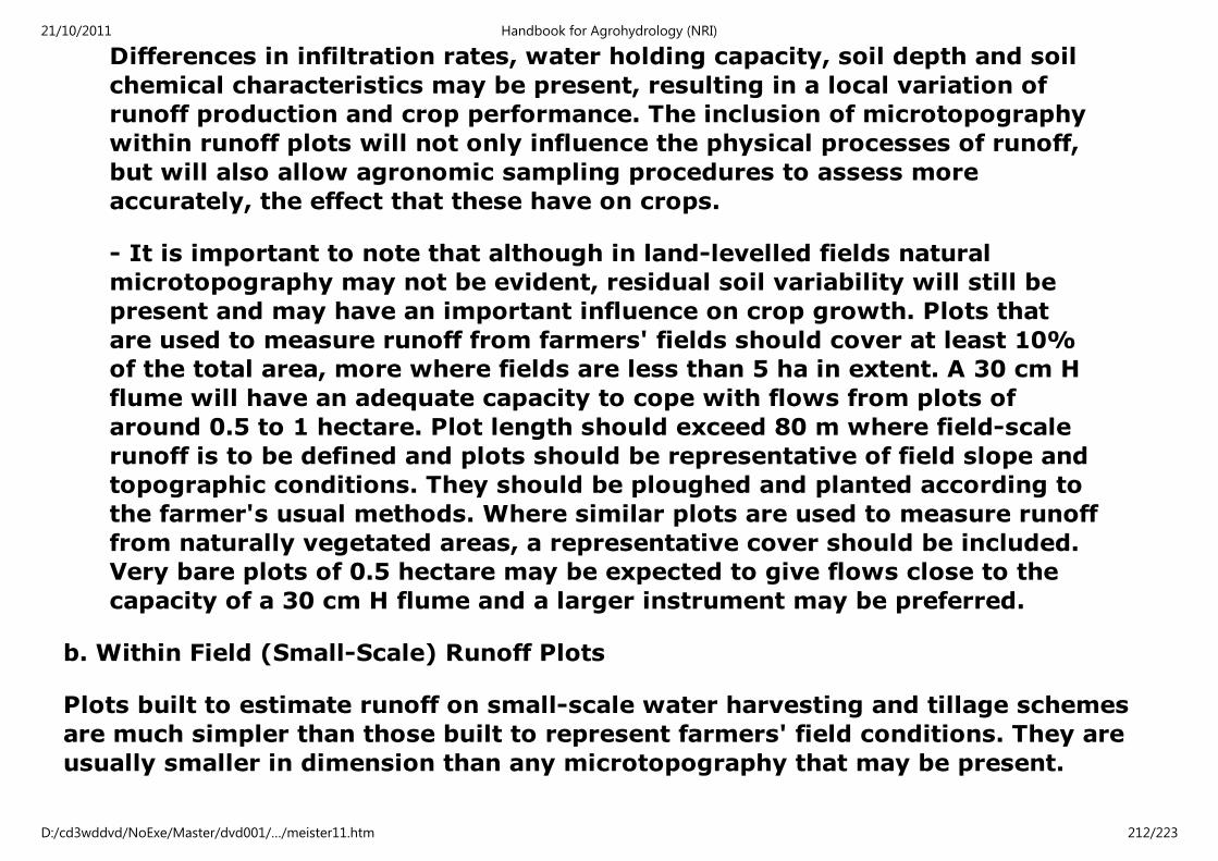
Differences in infiltration rates, water holding capacity, soil depth and soil
chemical characteristics may be present, resulting in a local variation of
runoff production and crop performance. The inclusion of microtopography
within runoff plots will not only influence the physical processes of runoff,
but will also allow agronomic sampling procedures to assess more
accurately, the effect that these have on crops.
- It is important to note that although in land-levelled fields natural
microtopography may not be evident, residual soil variability will still be
present and may have an important influence on crop growth. Plots that
are used to measure runoff from farmers' fields should cover at least 10%
of the total area, more where fields are less than 5 ha in extent. A 30 cm H
flume will have an adequate capacity to cope with flows from plots of
around 0.5 to 1 hectare. Plot length should exceed 80 m where field-scale
runoff is to be defined and plots should be representative of field slope and
topographic conditions. They should be ploughed and planted according to
the farmer's usual methods. Where similar plots are used to measure runoff
from naturally vegetated areas, a representative cover should be included.
Very bare plots of 0.5 hectare may be expected to give flows close to the
capacity of a 30 cm H flume and a larger instrument may be preferred.
b. Within Field (Small-Scale) Runoff Plots
Plots built to estimate runoff on small-scale water harvesting and tillage schemes
are much simpler than those built to represent farmers' field conditions. They are
usually smaller in dimension than any microtopography that may be present.
21/10/2011 Handbook for Agrohydrology (NRI)
D:/cd3wddvd/NoExe/Master/dvd001/…/meister11.htm 212/223

In these instances, it is usually not difficult to place plots to measure runoff on
any slope that is desired. Edge effects can be influential and it is important that
boundaries do not channel runoff to the collection tank in an unrealistic manner.
Rain falling directly into impermeable gutters, drains, etc. should be taken into
account.
Runoff will exploit very small elevation differences and sheet flow is quickly
converted into channel flow. If the aim of the experimentation is to promote the
even redistribution of runoff to the crop rooting zone, this is an important fact to
note.
Ploughed ridges and furrows play an important part in influencing runoff in these
circumstances and dead furrows may be a consequence of ploughing technique.
They can store a considerable amount of runoff (typically about 500 litres or 0.5
m³ per 10 m length) and their location can make a significant difference to runoff
measurement, especially for small runoff events.
It should be noted that such small plots may not behave as on the research station
if they are transferred and installed as extensive systems on farmers' field, where
pronounced microtopography may exist. The importance of placing runoff plots in
full knowledge of the effect of microtopography on runoff measurement cannot be
overstated.
In the first case (location Figure 6.8) average seasonal percent runoff from the
mounds was measured as 29.0 %, while the runoff from the crop plot (marked on
Figure 6.8) and which measures 100 m × 40 m, was only 4.5 % on average, over
three seasons. Slopes of the microtopography were about 5%, of the large plot
21/10/2011 Handbook for Agrohydrology (NRI)
D:/cd3wddvd/NoExe/Master/dvd001/…/meister11.htm 213/223

about 0.5%.
In the second case (location Figure 6.9), local runoff due to microtopography,
from the ridges to the channels, was in excess of 15% whereas average runoff
from four, 100 m × 40 m plots located on farmers' fields, but not shown in Figure
6.8, ranged from 1.7% to 4.5% over three seasons. Slopes from ridges to channels
ranged from about 3-8%,
large plots slopes were approximately 1%. If, in such cases, the results of runoff
measurement from the small plots were extrapolated to estimate net runoff values
from the whole field, they would lead to a gross over-estimation.
In practical terms this over-estimation might lead to the supposition that the
prevention of runoff was of paramount importance and costly (to the farmer in
terms of labour input for reward from increased yields) control measures might be
implemented. Where rainfall amounts are regarded as marginal for crop
production, these results might also suggest that additional supplementary water
should be obtained by water harvesting. The apparent runoff efficiencies of 15 -
29% indicate a high runoff efficiency, and it might be expected that an extra 100 -
125 mm per season could be provided on the basis of a 1:1 crop to water
harvesting area ratio. The actual runoff efficiencies of around 2 - 4% for the larger
plots show that this is not the case and 10 mm might represent the realistic
supplement that would be available for crops (ratio 1:1), unless the harvesting to
crop area ratio was very large.
Figure 6.10 shows a typical simple installation for the measurement of runoff from
field microtopography.
21/10/2011 Handbook for Agrohydrology (NRI)
D:/cd3wddvd/NoExe/Master/dvd001/…/meister11.htm 214/223

Figure 6.10: Installation to Measure Runoff from Field Microtopography
c. Natural Catchments
Natural catchments are usually larger than those that are artificially defined for
the purposes of runoff measurement. They frequently include areas with different
land slopes, soil textures, vegetation and microtopography. In areas with abrupt
changes in geology, different densities of stream networks are often exhibited.
21/10/2011 Handbook for Agrohydrology (NRI)
D:/cd3wddvd/NoExe/Master/dvd001/…/meister11.htm 215/223

Natural catchments are, therefore, more difficult to characterise than artificially
bounded catchments. For the purposes of study they may have to be divided into
subcatchments each with a more homogeneous nature. Runoff may then be
measured at locations to include each of these relatively homogeneous areas.
6.4 Field orientation
Field orientation is particularly important with regard to water conservation
measures that may be attempted on agricultural land. Fields are often defined
according to convenience, exploiting useful land marks such as the position of
roads and access, rivers and natural features. They are rarely oriented with runoff
losses and methods of runoff prevention in mind. Figure 6.11 shows a typical
semi-arid agricultural landscape.
A study of the photograph and the features of drainage shows that most fields are
oriented so that one corner is at the highest topographic elevation. Few of the
boundaries are parallel or at right angles to the overall land slope and the natural
drainage. In practical terms, this means that when a farmer ploughs, he or she will
always plough such that ridges and furrows provide channels that encourage
runoff. To plough along the contour would necessitate a start in the highest or
lowest corner, and ploughing for very short distances. The length of ploughing
would gradually increase until the full diagonal width of the field was attained,
then the distances would decrease until the farmer eventually reached the
opposite corner from where he or she had started. This would be a very difficult
and inefficient exercise from the viewpoint of ploughing, but cultivation would be
on the contour, disregarding local variations, and would inhibit the natural flow
direction of runoff. If contour bunding were to be practiced, similar difficulties
21/10/2011 Handbook for Agrohydrology (NRI)
D:/cd3wddvd/NoExe/Master/dvd001/…/meister11.htm 216/223

would be encountered.
The boundaries set for fields, in areas of agricultural activity where the effects of
urbanisation are small, are often those of roads and tracks. The directions of these
roads and tracks are not often exactly along the contour. They remove natural
vegetation, cross natural drainage systems, redirect runoff and concentrate it into
ditches, under culverts and bridges. This leads to the disruption of the natural
drainage, the concentration of flow and in many cases, serious problems of soil
erosion.
The problems of field orientation are complex. They involve land ownership, the
freedom of access and many other social issues, as well as a consideration of the
physical environment and the behaviour of drainage. The field studies of most
projects will be sited upon land that is already allocated and used for farming, so
few opportunities for the implementation of new allocations will exist. However,
the influence of field orientation is an important factor to note when field sites are
being selected and where the opportunity exists, serious consideration should be
given to the siting of new fields with a favourable aspect to natural drainage. The
problems of contour cultivation and the effects of local microtopography on such
practices are discussed in more detail in chapter 7, Water Harvesting.
6.5 Antecedent soil moisture conditions
Antecedent soil moisture conditions strongly influence the rate at which rainfall
infiltrates into the soil and contribute to the processes of runoff production. Soil
moisture levels at any time are the result of a combination of several factors,
mainly: the time elapsed since the last rainfall; the rainfall amount and intensity;
21/10/2011 Handbook for Agrohydrology (NRI)
D:/cd3wddvd/NoExe/Master/dvd001/…/meister11.htm 217/223

the climatic conditions that have prevailed since rainfall; the type and stage of
development of vegetation and soil texture and depth. Soil moisture levels can be
highly variable both between and within periods of a particular meteorological
activity. A high degree of spatial variability of soil moisture conditions may also be
encountered.
Soil moisture levels can be estimated by accounting procedures that balance the
infiltration of rainfall against losses by drainage and evapotranspiration. The
calculation of evapotranspiration (Et) by different methods is discussed in Chapter
8. A commonly used accounting procedure derives an Antecedent Precipitation
Index, by the application of an estimated factor for Et losses on previous rainfall.
It is generally assumed that the rate of reduction of the soil moisture reserves is
logarithmic, the rate falling as the availability of water decreases. The mechanisms
by which antecedent soil moisture effects runoff are highly variable from soil to
soil, but the general assumption equates higher proportions of runoff with higher
levels of soil moisture. This reflects the behaviour of infiltration rates under
increasingly moist conditions. Figure 6.12 illustrates changes in antecedent soil
moisture according to rainfall.
21/10/2011 Handbook for Agrohydrology (NRI)
D:/cd3wddvd/NoExe/Master/dvd001/…/meister11.htm 218/223

Figure 6.12: Change of Antecedent Soil Moisture Levels as shown by the
Antecedent Precipitation index
It is important early in a study to determine the precision to which antecedent soil
moisture needs to be measured or calculated. In situ measurements can be time-
consuming and calculations of Et usually necessitate the collection of a wide range
of meteorological information (see Chapter 8). General indicators of soil moisture
status may be adequate in some instances, but for use in, for example, regression
analysis against event runoff data, estimates of actual values are necessary.
6.6 Other catchment influences
21/10/2011 Handbook for Agrohydrology (NRI)
D:/cd3wddvd/NoExe/Master/dvd001/…/meister11.htm 219/223

a. Geology
Among the other influences on runoff that can be important is the geological
nature of the area under study. It affects runoff in three main ways:
1. Lithology. Particular rock types that are exposed at the surface of the ground
can have a profound influence on runoff, but generally large areas of exposed rock
are not common. Impermeable rock surfaces such as granite, gneisses, shales etc.
can produce very high percentages of surface flow and may be locally important as
sources of runoff. In semi-arid areas, and where these rocks are highly fractured,
they not only lead to rapid runoff from their impermeable surfaces, but can also
provide ground water that prolongs stream flow beyond the normally short period
of flash-flooding. Permeable lithologies such as limestone and porous sandstone
can limit surface flow to brief periods, only attained when ground water levels are
extremely high. Perennial springs may occur where they overlie impermeable
layers. According to its permeability, the geology of an area will determine surface
drainage density, stream channel length and catchment shape.
2. Soils. The most widespread effect on runoff, of geology, is through the type of
soil that it engenders. Granite, sandstones and quartzites produce sandy soils with
relatively few nutrients and high rates of infiltration. Shales and basic igneous
rocks usually give rise to relatively impermeable clays, though the humidity of the
climate will determine the processes of weathering and erosion, and the type of
soil that is subsequently formed.
3. Topography. Topography is also the result of geology and climate which
determine land form, slopes and local microtopography.
21/10/2011 Handbook for Agrohydrology (NRI)
D:/cd3wddvd/NoExe/Master/dvd001/…/meister11.htm 220/223

b. Stream Density
Stream density is an index of the concentration of a drainage network within a
catchment area. It will not be an important factor when small runoff plots are
studied, but is used frequently as an independent variable in regression analysis
for natural catchments. It should be noted that larger runoff plots, for instance
those greater than about 0.5 hectare especially where they constitute a portion of
a large field or a natural catchment, may well exhibit a stream network, though in
arid and semi arid regions stream flow will be ephemeral. Such networks exhibit
themselves as microtopography and may be influential in determining the runoff
efficiency of the catchment, as they intercept sheet flow and channel it to the
catchment outlet. The measurement of discharge by sheet flow alone is more
difficult to achieve, as it is prone to retention by vegetation, ponding and
subsequent infiltration. In origin, stream density is closely related to structural
geology, Ethology, slope and climate. In general terms the greater the density of a
stream network, the greater the percentage runoff for any given rainfall, because
stream channels conduct runoff efficiently they lead to high, sharp peaks and rapid
recessions. Relatively complicated systems of stream hierarchy are used to derive
a stream density index in hydrological analysis, but they are somewhat beyond the
scope of this book. A simple but appropriate index that can be used for regression
analysis is length of stream per unit area (e.g. km km-2), though the correlation of
such a stream index with other catchment characteristics must be considered
before use in regression.
c. Human Factors and Agriculture
Human influences on runoff can be very great and they work at many scales. The
21/10/2011 Handbook for Agrohydrology (NRI)
D:/cd3wddvd/NoExe/Master/dvd001/…/meister11.htm 221/223

wholesale destruction of huge forested areas has led to disastrous flooding and
extreme environmental degradation. A list of the most important influences that
affect the amount of runoff from the land may include:
Urbanisation
Deforestation
Overgrazing
Dam building
Canalisation
Reduction of flood plains
Draining of marshes and swamps
Arable agriculture appears less harmful, perhaps, but its effect on the hydrological
nature of much of he world's surface is profound.
Equipment costs
All costs of locally made equipment are approximate. The costs of raw materials
and especially labour are highly variable from country to country, but a good idea
of cost magnitude can be gained from the figures quoted below. The costs of
manufactured equipment are based on 1993 prices. Shipping, agents' fees and
fluctuations in exchange rate cannot be taken into account.
Item Typical Approximate Cost in $ US
2 - 3 Seat light aircraft per hour 300 - 500
4 - 5 Seat with global navigation per hour 400 - 700
(sufficient to cover 2 -3 sites within about 30 km radius)
21/10/2011 Handbook for Agrohydrology (NRI)
D:/cd3wddvd/NoExe/Master/dvd001/…/meister11.htm 222/223

(sufficient to cover 2 -3 sites within about 30 km radius)
Wheel point apparatus 1 30 - 60
21/10/2011 Handbook for Agrohydrology (NRI)
D:/cd3wddvd/NoExe/Master/dvd001/…/meister11.htm 223/223


![[NRI] Report](https://static.fdocuments.net/doc/165x107/568c3c231a28ab0235acd82c/nri-report-56f2c44cdd788.jpg)