HANDBOOK – DIGITAL RADIO-RELAY SYSTEMS · 2018-05-25 · - 1 - CHAPTER 1 INTRODUCTION 1.1 Intent...

- iii -

TABLE OF CONTENTS

Page

CHAPTER 1 - INTRODUCTION ........................................................................................ 1

1.1 INTENT OF HANDBOOK ..................................................................................... 1

1.2 EVOLUTION OF DIGITAL RADIO-RELAY SYSTEMS .................................... 2

1.3 DIGITAL RADIO-RELAY SYSTEMS AS PART OF DIGITALTRANSMISSION NETWORKS............................................................................. 3

1.4 GENERAL OVERVIEW OF THE HANDBOOK .................................................. 5

1.5 OUTLINE OF THE HANDBOOK.......................................................................... 5

CHAPTER 2 - BASIC PRINCIPLES .................................................................................. 7

2.1 DIGITAL SIGNALS, SOURCE CODING, DIGITAL HIERARCHIESAND MULTIPLEXING .......................................................................................... 7

2.1.1 Digitization (A/D conversion) of analogue voice signals ........................... 72.1.2 Digitization of video signals........................................................................ 82.1.3 Non voice services, ISDN and data signals ................................................. 82.1.4 Multiplexing of 64 kbit/s channels .............................................................. 82.1.5 Higher order multiplexing, Plesiochronous Digital Hierarchy (PDH) ........ 82.1.6 Other multiplexers ....................................................................................... 112.1.7 Synchronous multiplexing, Synchronous Digital Hierarchy (SDH)............ 11

2.1.7.1 General principles.......................................................................... 112.1.7.2 Synchronous multiplexing scheme................................................ 122.1.7.3 Overhead functions........................................................................ 152.1.7.4 The Sub-STM-1 signal format ...................................................... 162.1.7.5 ATM transport in the SDH, SDH transport via PDH signals ........ 18

2.1.8 Interconnection at baseband, physical interface characteristics .................. 192.1.9 Jitter and wander timing and synchronization ............................................. 20

2.2 FUNDAMENTALS OF TERRESTRIAL DIGITAL RADIO-RELAYSYSTEMS ............................................................................................................... 20

2.2.1 Architecture of digital radio-relay systems.................................................. 222.2.1.1 Digital transmitter ......................................................................... 222.2.1.2 Digital receiver .............................................................................. 242.2.1.3 Radio transmitter and receiver ...................................................... 262.2.1.4 Channel combining and antenna considerations ........................... 282.2.1.5 Radio switching section ................................................................ 29

References to Chapters 1 and 2................................................................................................ 32

- iv -

CHAPTER 3 - LINK DESIGN CONSIDERATIONS ........................................................ 34

3.1 APPLICATIONS OF DIGITAL RADIO-RELAY SYSTEMS ............................... 34

3.1.1 General ....................................................................................................... 343.1.2 Available frequency bands .......................................................................... 353.1.3 Coexistence between analogue and digital radio systems ........................... 383.1.4 Digital channel capacity .............................................................................. 393.1.5 Digital networks .......................................................................................... 41

3.1.5.1 Long haul digital radio systems ..................................................... 413.1.5.2 Short haul digital radio systems .................................................... 413.1.5.3 Digital radio access networks ........................................................ 42

3.1.6 Radio Local Area Networks (RLAN).......................................................... 423.1.6.1 General .......................................................................................... 423.1.6.2 Frequency bands ............................................................................ 433.1.6.3 Multiple access and modulation .................................................... 433.1.6.4 System configuration..................................................................... 443.1.6.5 Examples of RLANs ..................................................................... 45

3.2 PERFORMANCE AND AVAILABILITY OBJECTIVES..................................... 46

3.2.1 Hypothetical digital connection, path and section ....................................... 463.2.2 Error performance parameters and objectives ............................................. 47

3.2.2.1 Error performance parameters and objectives based on ................ 47ITU-T Recommendation G.821 .................................................... 47

3.2.2.2 Error performance parameters and objectives based onITU-T Recommendation G.826 .................................................... 49

3.2.3 Availability performance parameters and objectives .................................. 543.2.4 Bringing-into-service and maintenance ....................................................... 57

3.2.4.1 Relationship between performance limits and objectives ............. 583.2.4.2 Performance limits for bringing-into-service ................................ 59

3.3 UPGRADING FROM ANALOGUE TO DIGITAL RADIO SYSTEMS............... 60

3.3.1 Advantages of a new digital microwave system.......................................... 603.3.2 Existing analogue microwave system characteristics .................................. 623.3.3 Difficult digital microwave paths ................................................................ 623.3.4 Antenna feeder systems ............................................................................... 633.3.5 Digital microwave system overbuild ........................................................... 633.3.6 Analogue/digital RF coupling arrangements ............................................... 633.3.7 Analogue spur links ..................................................................................... 643.3.8 Analogue-to-digital circuit cutover phases.................................................. 643.3.9 The circuit cutover....................................................................................... 64

3.4 RF CHANNEL ARRANGEMENTS....................................................................... 65

3.4.1 Introduction ................................................................................................. 653.4.2 Spectrum related parameters ....................................................................... 653.4.3 Type of channel arrangement ...................................................................... 663.4.4 Homogeneous pattern and channel subdivision .......................................... 693.4.5 Intra-system and inter-system interference criteria...................................... 70

- v -

3.5 BAND SHARING WITH OTHER SERVICES ...................................................... 73

3.5.1 Assessment of interference from other services .......................................... 733.5.1.1 General .......................................................................................... 73

` 3.5.1.2 Degradation in performance and availability ................................ 733.5.1.3 Assessment of aggregate effects of interference from various

sources ........................................................................................... 753.5.2 Basic parameters for sharing considerations ............................................... 77

3.5.2.1 Receiver side ................................................................................. 773.5.2.2 Transmitter side ............................................................................. 79

3.5.3 Status of studies on frequency sharing within RadiocommunicationStudy Group 9.............................................................................................. 82

References to Chapter 3............... ............................................................................................ 83

CHAPTER 4 - DESIGN PARAMETERS ........................................................................... 86

4.1 PROPAGATION RELATED ISSUES.................................................................... 86

4.1.1 Concept of free space loss ........................................................................... 864.1.2 Visibility ...................................................................................................... 87

4.1.2.1 Refractive aspects .......................................................................... 874.1.2.2 Path profiles, clearance and obstructions ...................................... 914.1.2.3 Diffraction aspects ......................................................................... 93

4.1.3 Surface reflection......................................................................................... 984.1.3.1 Introduction ................................................................................... 984.1.3.2 Specular reflection from a plane Earth surface ............................. 984.1.3.3 Specular reflection from a smooth spherical Earth ....................... 984.1.3.4 A practical method to determine specular ground reflections ....... 102

4.1.4 Atmospheric multipath ................................................................................ 1034.1.4.1 Introduction ................................................................................... 1034.1.4.2 Fading due to multipath and related mechanisms ......................... 1044.1.4.3 Atmospheric multipath modelling ................................................. 1104.1.4.4 Outage computation methods ........................................................ 116

4.1.5 Precipitation attenuation .............................................................................. 1194.1.6 Scattering property ...................................................................................... 123

4.1.6.1 Rain scattering ............................................................................... 1234.1.6.2 Terrain scattering ........................................................................... 124

4.1.7 Polarization.................................................................................................. 1244.1.7.1 General aspects .............................................................................. 1244.1.7.2 Explanation for XPD degradation mechanisms ............................ 1254.1.7.3 Computation of cross-polarization degradation ............................ 126

4.1.8 Gaseous attenuation..................................................................................... 128

4.2 EQUIPMENT RELATED ASPECTS ..................................................................... 131

4.2.1 Baseband processing.................................................................................... 1314.2.1.1 General baseband processing function .......................................... 1314.2.1.2 Radio specific processing functions for baseband signals ............ 133

- vi -

4.2.2 Modulation and demodulation..................................................................... 1354.2.2.1 Basic principles ............................................................................. 1354.2.2.2 Linear modulation schemes ........................................................... 1364.2.2.3 Non-linear modulation schemes .................................................... 1384.2.2.4 Coded modulation ......................................................................... 1394.2.2.5 Spectrum shaping .......................................................................... 1414.2.2.6 Probability of error for the additive white Gaussian noise channel . 1464.2.2.7 Aspects relevant to demodulation process .................................... 1504.2.2.8 Modem functional blocks .............................................................. 159

4.2.3 Transmitter .................................................................................................. 1684.2.3.1 Local oscillator (LO) ..................................................................... 1684.2.3.2 Frequency conversion in the mixer ............................................... 1694.2.3.3 Transmission power versus peak factor and modulation format

“(back-off)” with and without linearisation .................................. 1704.2.3.4 Power amplifier ............................................................................. 1704.2.3.5 Spurious emissions (types and requirements) internal/external) ... 1744.2.3.6 Linearisation (requirements and techniques)................................. 1744.2.3.7 Filtering (RF/IF) ............................................................................ 177

4.2.4 Receiver ....................................................................................................... 1774.2.4.1 Frequency conversion .................................................................... 1774.2.4.2 Filtering ......................................................................................... 1784.2.4.3 Noise figure ................................................................................... 1814.2.4.4 Required bandwidth ...................................................................... 1824.2.4.5 Signature........................................................................................ 182

4.2.5 Radio protection switching.......................................................................... 1824.2.5.1 General .......................................................................................... 1824.2.5.2 Types of protection arrangements ................................................. 1824.2.5.3 Architecture of radio protection switching .................................... 1834.2.5.4 Protection switching on set stand-by basis .................................... 1844.2.5.5 Multi-line switching ...................................................................... 1844.2.5.6 Factors influencing the choice of switching criteria...................... 1854.2.5.7 Calculation of link unavailability .................................................. 186

4.2.6 Antennas and feeder systems....................................................................... 1864.2.6.1 Fundamentals of radio-relay antennas ........................................... 1864.2.6.2 Parabolic antenna .......................................................................... 1904.2.6.3 Horn reflector antenna ................................................................... 1934.2.6.4 High performance antenna ............................................................ 1944.2.6.5 Fundamentals of feeder systems .................................................... 1974.2.6.6 System multiplexing filter ............................................................. 203

4.3 COUNTERMEASURES ......................................................................................... 205

4.3.1 General explanation..................................................................................... 2054.3.1.1 Purpose of countermeasures .......................................................... 2054.3.1.2 Classification of countermeasures ................................................. 2064.3.1.3 Evaluation of countermeasures ..................................................... 208

- vii -

4.3.2 Adaptive equalization .................................................................................. 2084.3.2.1 Basic principles ............................................................................. 2084.3.2.2 Equalization structures .................................................................. 2094.3.2.3 Adaptation algorithms ................................................................... 211

4.3.3 Interference cancellers ................................................................................. 2144.3.3.1 Basic principles ............................................................................. 2144.3.3.2 Interference cancellers ................................................................... 2154.3.3.3 Cross-polarization interference cancellers .................................... 216

4.3.4 Adaptive transmitter power control ............................................................. 2194.3.4.1 Basic principles ............................................................................. 2194.3.4.2 Applications .................................................................................. 220

4.3.5 Data coding and error correction ................................................................. 2214.3.5.1 Forward error correction................................................................ 2214.3.5.2 Coded modulation ......................................................................... 222

4.3.6 Space diversity............................................................................................. 2304.3.6.1 Basic principles ............................................................................. 2304.3.6.2 Methods of obtaining diversity signals.......................................... 2314.3.6.3 Signal control methods .................................................................. 2344.3.6.4 Improvement effects ...................................................................... 2384.3.6.5 Triple and quadruple diversity....................................................... 247

4.3.7 Angle diversity ............................................................................................ 2524.3.7.1 Basic principles ............................................................................. 2524.3.7.2 Applications .................................................................................. 252

4.3.8 Polarization diversity................................................................................... 2564.3.9 Frequency diversity ..................................................................................... 257

4.3.9.1 Concept of frequency diversity...................................................... 2574.3.9.2 Improvement effect ....................................................................... 257

4.3.10 Synergistic effects........................................................................................ 2594.3.10.1 Space diversity and adaptive equalizers ........................................ 2594.3.10.2 Space and frequency (hybrid) diversity ......................................... 261

4.3.11 Multi-carrier transmission ........................................................................... 262


CHAPTER 5 - LINK ENGINEERING................................................................................ 273

5.1 GENERAL NETWORK AND LINK DESIGN CONSIDERATIONS ................... 273

5.1.1 Performance objectives and network planning aspects ............................... 2735.1.2 Link and hop design objectives ................................................................... 273

5.2 PRELIMINARY RADIO ROUTE AND SITE SELECTION................................. 274

5.2.1 Introduction ................................................................................................. 2745.2.2 Contour maps .............................................................................................. 2745.2.3 Identification of route alternatives............................................................... 2745.2.4 Use of existing infrastructure and site sharing ............................................ 2755.2.5 Preliminary path profiles ............................................................................. 2755.2.6 Preliminary performance prediction calculations ........................................ 276

- viii -

5.2.7 Selection of route alternatives ..................................................................... 2765.2.8 Cost assessment ........................................................................................... 2765.2.9 Selection of “best route alternatives” .......................................................... 2765.2.10 Field surveys................................................................................................ 276

5.2.10.1 The purpose of field surveys ......................................................... 2765.2.10.2 Location of sites, obstacles and roads ........................................... 2775.2.10.3 Geographical characteristics of roads and sites ............................. 2775.2.10.4 Survey of the terrain in between sites............................................ 2775.2.10.5 Additional issues regarding surveys of existing stations ............... 2775.2.10.6 Survey reporting ............................................................................ 278

5.2.11 Final radio route and site selection .............................................................. 278

5.3 LINK DESIGN PROCEDURES ............................................................................. 278

5.3.1 Introduction ................................................................................................. 2785.3.2 Error performance and availability objectives............................................. 2795.3.3 Frequency band and channel selection ........................................................ 281

5.3.3.1 Frequency band characteristics ...................................................... 2815.3.3.2 Frequency band and channel selection .......................................... 282

5.3.4 Path engineering .......................................................................................... 2825.3.4.1 General considerations .................................................................. 2825.3.4.2 Free-space propagation, receiver threshold, system gain and flat

fade margin .................................................................................... 2825.3.4.3 Outage time prediction for single frequency clear air fading ........ 283

5.3.5 Interference considerations .......................................................................... 2855.3.5.1 Spectrum masks and cross-polarization discrimination (XPD) .... 2855.3.5.2 The threshold-to-interference ratio................................................ 285

5.3.6 Outage prediction for rain............................................................................ 2895.3.7 Short-hand design guide .............................................................................. 291

5.4 LINK AVAILABILITY ENGINEERING ............................................................... 293

5.4.1 Introduction ................................................................................................. 2935.4.2 Factors affecting availability ....................................................................... 2935.4.3 Apportionment of availability objectives .................................................... 2935.4.4 Equipment contribution to unavailability .................................................... 2945.4.5 Effectiveness of maintenance arrangements................................................ 2945.4.6 Calculation of equipment unavailability...................................................... 2955.4.7 Clear air propagation contribution to unavailability.................................... 2955.4.8 Rain-induced unavailability......................................................................... 2955.4.9 Use of redundancy to improve link availability .......................................... 2965.4.10 Calculation of link unavailability ................................................................ 296

ANNEXES to Chapter 5 - Performance prediction methods................................................... 297

Introduction.............................................................................................................................. 297

- ix -

ANNEX I to Chapter 5 - Performance prediction, method 1 (fade margin method)............... 298

5.I.1 Introduction ................................................................................................. 2985.I.2 Single frequency fading ............................................................................... 2995.I.3 Broadband or dispersive fading ................................................................... 301

5.I.3.1 A channel model ............................................................................ 3015.I.3.2 Equipment signature ...................................................................... 3035.I.3.3 Radio outage due to dispersive effects .......................................... 3065.I.3.4 Scaling of signatures with symbol rate .......................................... 3065.I.3.5 Results of propagation measurements ........................................... 307

5.I.4 The total outage ........................................................................................... 3085.I.5 Outage time reduction achieved by diversity systems ................................. 309

5.I.5.1 The concept of dispersive fade margin .......................................... 3095.I.5.2 Relationship with the Bellcore dispersive fade margin ................. 3105.I.5.3 Outage time reduction by diversity systems .................................. 3115.I.5.4 Space diversity and frequency diversity improvement factors ...... 3125.I.5.5 Total outage time in diversity systems .......................................... 312

5.I.6 Outage time reduction achieved by equalizers ............................................ 3125.I.7 Combined use of equalizer and diversity - the synergistic effect ................ 313

ANNEX II to Chapter 5 - Performance prediction, method 2 (normalized signature method)... 314

5.II.1 Flat fade margin and noise contribution ...................................................... 3145.II.1.1 Noise budget assignment ............................................................... 3145.II.1.2 Calculation of noise component .................................................... 317

5.II.2 Dispersive fade margin based on normalized signature method ................ 3195.II.3 Improvement of outage probability by countermeasures............................. 321

5.II.3.1 General .......................................................................................... 3215.II.3.2 Examples of improvement factors ................................................. 321

5.II.4 General assessment procedure..................................................................... 322

ANNEX III to Chapter 5 - Performance prediction, method 3 (“Linear amplitude dispersion”(LAD) statistics method) ......................................................................................... 324

5.III.1 Basis of the method ..................................................................................... 3245.III.2 The fading model, parameter distributions and assumptions ...................... 3255.III.3 Signature scaling and normalised system parameters ................................. 3265.III.4 Outage prediction for non-diversity............................................................. 3275.III.5 Outage prediction for diversity.................................................................... 3285.III.6 Simplified outage prediction for non-diversity and diversity...................... 3295.III.7 Example application of the prediction method and comparison with

measurements .............................................................................................. 3305.III.8 Linear amplitude dispersion (LAD)/in-band (IBAD) method ..................... 331

5.III.8.1 Experimental validation of the method ......................................... 3315.III.8.2 Measured variations of LAD ......................................................... 331


- x -

CHAPTER 6 - OPERATIONS AND MAINTENANCE .................................................... 338

6.1 SYSTEM MAINTENANCE AND ADMINISTRATION ...................................... 338

6.1.1 Maintenance strategy ................................................................................... 3386.1.2 Commissioning and acceptance tests .......................................................... 3386.1.3 Bringing-into-service................................................................................... 340

6.1.3.1 Reference performance objectives ................................................ 3406.1.3.2 BIS limits ....................................................................................... 3416.1.3.3 Calculation of BIS limits ............................................................... 342

6.1.4 Maintenance ................................................................................................ 3436.1.4.1 Maintenance limits ........................................................................ 3446.1.4.2 Fault detection and localization..................................................... 3456.1.4.3 Fault localization information ....................................................... 3456.1.4.4 Fault localization procedures on digital transmission system ....... 347

6.1.5 Alarms ....................................................................................................... 3496.1.5.1 Alarms under pre-ISM conditions ................................................. 3496.1.5.2 Alarms under in-service measurement (ISM) conditions.............. 350

6.1.6 Service channels .......................................................................................... 3516.1.7 Protection switching .................................................................................... 3526.1.8 Digital radio-relay systems in a telecommunication management network ... 352

6.2 MEASUREMENTS................................................................................................. 354

6.2.1 Introduction ................................................................................................. 3546.2.2 Basic criteria for bit error performance evaluation...................................... 3556.2.3 OOS measurements ..................................................................................... 359

6.2.3.1 PRBS test signals .......................................................................... 3596.2.3.2 PRBS generator and error detector ................................................ 3616.2.3.3 Framed digital signal test pattern .................................................. 3616.2.3.4 Block-oriented error performance measurements ......................... 3626.2.3.5 Block sizes for performance measurements on PDH systems ...... 3626.2.3.6 Block sizes for performance measurements on SDH systems ...... 363

6.2.4 ISMs ....................................................................................................... 3666.2.4.1 PDH path performance monitoring ............................................... 3666.2.4.2 External monitoring equipment with tributary stream .................. 3666.2.4.3 Built-in monitoring systems .......................................................... 3676.2.4.4 Test sequence interleaving ............................................................ 3676.2.4.5 Parity-check coding ....................................................................... 3676.2.4.6 Cyclic code error detection ............................................................ 3686.2.4.7 Code-violations detection.............................................................. 3696.2.4.8 FEC facilities ................................................................................. 3696.2.4.9 Pseudo-error detection................................................................... 3696.2.4.10 ISM of PDH paths in conjunction with

ITU-T Recommendation G.826................................................ 3696.2.4.11 ISM of SDH paths ......................................................................... 372

6.2.5 Practical considerations in making in-service performance measurements ... 3746.2.5.1 Monitors used for equipment maintenance and protection ........... 3756.2.5.2 Monitors for checking network performance objectives ............... 375

- xi -

6.2.6 Jitter and wander measurements.................................................................. 3766.2.6.1 Input jitter tolerance measurement ................................................ 3776.2.6.2 Output jitter measurement ............................................................. 3786.2.6.3 Jitter transfer characteristics .......................................................... 3786.2.6.4 Wander measurements .................................................................. 378

6.2.7 Digital radio-relay equipment measurement ............................................... 3796.2.7.1 Equipment signature ...................................................................... 3796.2.7.2 Cross-polarization interference cancellers .................................... 381


LIST OF ABBREVIATIONS .................................................................................................. 389

- xiii -

INTRODUCTION

I am very pleased to introduce this first edition of the Handbook on digital radio-relaysystems, prepared by a group of experts from Radiocommunication Study Group 9 under thechairmanship of Dr. Rudolf Hecken (United States of America). The Handbook provides a detailedcoverage of the state-of-the-art in present-day, high usage, digital microwave transmission equipmentand offers some insight into present and future technological trends. It consists of 6 chapters whichdescribe the basic principles, propagation and layout considerations, design parameters, linkengineering, operation and maintenance of radio-relay systems. Many references are also providedthat can be consulted, if needed, for additional details.

According to Resolution ITU-R 12 of the ITU Radiocommunication Assembly “inestablishing priorities for the preparation and publishing of handbooks, special consideration shouldbe given to the needs of developing countries”. Considering the particular importance of radio-relaysystems in developing countries, this Handbook was developed under Radiocommunication StudyGroup 9 Decision 110. To assist administrations and organizations in the preparation of programmesand the education of personnel, the Handbook includes detailed tutorial texts. Telecommunicationoperators, particularly new operators, will also find valuable information for the planning anddeployment of modern radiocommunication networks, covering both terrestrial point-to-point andpoint-to-multipoint links.

Although several publications on radio-relay systems are currently available on the market,radiocommunication applications, techniques and practices are evolving rapidly. This Handbook’sinclusion of fundamental information formerly in various ITU-R Reports, together with the mostrecent developments in radio-relay systems, will make this comprehensive publication anindispensable reference for radiocommunication engineers.

Robert W. JonesDirector,

Radiocommunication Bureau

- xv -

FOREWORD

Over the past decade or so, national and international telecommunication have beenundergoing a dramatic evolution and transformation in regard to technology, application, scale andpublic policy. One of the foremost driving forces is the liberalization of the telecommunicationmarket from monopolistic or government controlled structures. This shift in public policy has set thestage for the emergence of new enterprises that compete fiercely in the telecommunications marketplace. A further accelerating factor in this period of change has been the rapid innovation in digitaltechnology that continues to perfect the movement and management of information to increasinglyhigher levels of performance and reliability. At the same time, the immense thrust in digitalprocessing capability with its ever-decreasing cost spawns new applications and services almostdaily. Prime examples are the phenomenal growth of mobile communications and new wirelesssystems as well as the increasing number of corporate communication networks. Still two morepotent agents in this progressive transformation must be mentioned: these are the enormousexpansion of world trade along with the ending of the cold war. Clearly, both factors are driving thetelecommunications market to a new, truly global scale.

Digital radio relay systems have become in many ways a central part in this evolutionaryprocess. In mobile communications they are heavily deployed for the economical interconnection ofbase stations. Similar utilization is predicted for the emerging personal wireless networks. Digitalradio links are used for connecting islands of local area networks to backbone trunks, either tobecome part of national or international private networks or to provide access to public switchednetworks. It is gratifying also to see ever increasing deployment of digital radio relay systems indeveloping countries as well as in sparsely populated regions, providing affordable means oftelecommunications for many.

The Radiocommunication Sector of the International Telecommunications Union and itspredecessor, the International Radio Consultative Committee (CCIR) have played a decisive role inguiding telecommunication operators and the pertinent industries towards the most efficient use ofthe microwave spectrum and towards continuous performance enhancements in quality of serviceand link reliability. These guidelines are issued as Recommendations and - in the past - in the form ofReports as an additional official publication. However, at the 1990 Radiocommunication Assemblyof the former CCIR it was decided to discontinue the publication of existing Reports. It was thenrecommended to either convert these Reports to Recommendations or make them part of aHandbook. In its November 1991 meeting ITU-R Study Group 9 took the initiative and decided toform an expert group with the charter to create and publish a Handbook on Digital Radio-RelaySystems based on up-to-date information and existing Reports and Recommendations.

The Handbook Group met for the first time in December of 1992 and thereafter annuallyuntil March of 1996. In spite of a heavy load of unrelated work at their home location, the voluntarymembers of this group were able to complete all the technical writing essentially by mid-1996. AsChairman of the Handbook Group throughout this project, I wish to thank the individual authors andcontributors for their unceasing effort and great cooperation. My gratitude goes also to all sponsoringorganizations that provided continuing support and the necessary funding for our endeavor.

- xvi -

My special thanks go to Dr. Murotani and the Mitsubishi Electric Company of Japan in providing aspecial fund to hire experts for certain sections of the Handbook or for aiding in technical editing.Without this financial support a timely completion of the Handbook would not have been possible.

Members of the Handbook Group came from eleven countries and it is with pleasure andgratitude that I individually acknowledge their personal contributions as well as their sponsors:

Australia (L. Davey, Telecom Australia), Canada (D. Couillard, Harris Farinon), Denmark(E. Stilling, Carl Bro. International Consulting), France (L. Martin, France Telecom), France(G. Karam, S.A.T.), Germany (H.-J. Thaler, Siemens A.G.), Germany (H. Reissmann, DeutscheTelekom), India (V. Mitra, Ministry of Telecommunications), Italy (U. Casiraghi, Alcatel-Telettra),Italy (M. Zaffaroni, Italtel S.p.A), Japan (A. Hashimoto, NTT), Japan (T. Ozaki, Fujitsu), RussianFederation (V. Minkin, NIIR), Russia Federation (L.M. Martinov, Ministry of Communications),United Kingdom (G.D. Richman, British Telecom), United States of America (A. Giger, LucentTechnologies - Bell Laboratories).

Especially, I would like to thank Mr. Lorenzo Casado of the Radiocommunication Bureau(BR) for his countless hours of extra work and dedication to this project. His assistance as principalcoordinator and organizer of our meetings in Geneva has been most effective and invaluable. Equallyexceptional has been Mr. Casado's attention to all the details in coordinating the enormous amount ofprocessing of all the documents, to personally take care of graphics as well as final editing and tosupervise the necessary translations into French and Spanish. Last but not least, I also want toexpress my gratitude to the BR staff and the editing group at the ITU for their support of the manydifficult and exhausting tasks that were necessary to accomplish our challenging goals in such a shortperiod of time. This Handbook would not have been successful without their full commitment.

Rudolf P. HeckenChairman

Handbook Group on Digital Radio-Relay Systems

- xvii -

PREFACE

The present Handbook is published mainly to assist planners and decision-makers in thedeployment of digital radio-relay systems. It has been prepared for tutorial purposes by a group ofexperts within Radiocommunication Study Group 9 and is relatively easy to understand so that it canbe used to update knowledge and training of young engineers in industrialized and developingcountries.

During the last decade, radiocommunication technologies have experienced a tremendousevolution, particularly for radio-relay systems of the terrestrial fixed service, one of the pioneers inradiocommunications. It has been necessary to reduce the cost and size of equipment whilstsimultaneously considerably enhancing performance and availability to better facilitate challengingother modern wired means of transmission, such as fibre optics. The Handbook provides material onthe present and future technological trends in digital radio-relay systems.

Telecommunication, particularly for low populated rural areas and new access networkrequirements, should be provided, as much as possible, through very inexpensive telecommunicationlinks, in order to minimize costs and achieve a quick return on investment. Informative materials foracquiring comprehension in propagation aspects, modulation techniques, system design, operationand maintenance of digital radio-relay systems are illustrated in the Handbook. It will be most usefulwhen establishing new radiocommunication systems by offering a flexible and rapid choicecompared to other available means.

I trust this Handbook will be of significant assistance for those readers desiring to captureand understand the fascinating world of radiocommunications.

Masayoshi MurotaniChairman

Radiocommunication Study Group 9

- 1 -

CHAPTER 1

INTRODUCTION

1.1 Intent of Handbook

During their autumn meeting in Geneva from 5 to 8 November 1991, former CCIR (see Note 1) Study Group 9 decided to establish a Handbook Group. As documented in Decision 110, the charter for the Handbook Group was to prepare a Handbook on Digital Radio-Relay Systems in order to “provide administrations and organizations with tutorial documents to assist them in the preparation of their programmes and in the education of their personnel”. Decision 110 explicitly stated the importance of digital radio-relay systems in developing countries. It further declared that advances in the technology would justify the preparation of the Handbook on Digital Radio-Relay Systems. One other major aspect of this decision was the proclamation that some text from existing Reports in the Annex to Volume IX-1 (Düsseldorf 1990) would not be converted to Recommendations and would, therefore, be more properly used as the material in the Handbook.

NOTE 1 – In 1993, the CCIR was officially renamed ITU Radiocommunication Sector (ITU-R).

In the context of this Handbook, digital radio-relay systems include the equipment, the propagation channel, and operational tools necessary for the terrestrial transport of digitally encoded information using electromagnetic waves at microwave frequencies.

A Handbook, as defined in Resolution ITU-R 1, § 6.1.7 and adopted by the 1995 Radiocommunication Assembly, is “a text which provides a statement of the current knowledge, the present position of studies, or of good operating or technical practice, in certain aspects of radiocommunications”. With this definition and the charter in mind, the Handbook Group consisting of experts of eleven member countries met for the first time during the spring of 1992 in Geneva. At that time a first working outline of the Handbook was established and the contents of the book were refined in several subsequent meetings. During this time the Group has produced a most valuable document. Its practical value shall prove itself during the design and development of new microwave links of any capacity and in any frequency bands.

Contributions to the book in its present form came from international experts most of whom have been associated with ITU-R for many years. They have considerable practical as well as scientific knowledge of the physical principles and current technologies that play a critical role in the design of digital radio links. The breadth of their expertise ranges from link design to operations and maintenance methods.

To be applicable in any part of the world, it is expected that this Handbook will be useful for engineers and technicians of operators of digital radio-relay systems. Most importantly, the Handbook will be invaluable for administrations in many countries relying on digital radio-relay systems as one of their means for providing high quality digital transmission in their communications networks.

- 2 -

1.2 Evolution of digital radio-relay systems

The history of radio-relay systems began in 1947 with the installation of the first experimental radio-relay link by Bell Laboratories between New York and Boston. This analogue system (TD-X) utilized vacuum tubes for signal amplification and employed frequency modulation (FM). From this experimental system evolved the 4 GHz TD-2 system that in 1950 carried the first commercial telephony service. Through continuous improvements and technological advancements, this system would expand by 1960 into a national long distance network connecting the East and West coast of the United States of America. This route had a total length of about 6 500 km with 125 active repeater stations.

Several key elements and characteristics of the TD-2 system did set standards to which manufacturers of long-haul and short-haul radio systems would adhere for some time to come. This permitted the introduction of a new transmission technology in many countries that was capable of carrying a large number of voice circuits over considerable distances. In competition with the existing transmission media this new technology improved the quality of voice transmission significantly.

Beginning in the early 1950s, microwave radio systems similar to TD-2 were installed outside the United States of America on major backbone routes in Australia, Canada, France, Italy and Japan. National manufacturers began developing improved systems based on their own research and new requirements. Important aspects of this research were extended into studies by the CCIR leading to many Recommendations. By 1979, channel capacities of commercial systems reached 3 600 voice circuits in Japan and by 1980, 6 000 analogue voice circuits in the United States of America. By employing single sideband modulation, the AR6A system packed these 6 000 circuits within the 30 MHz wide channels of the 6 GHz band. Although these high capacities lowered transmission cost per circuit to an all-time low, it was the advent of digital technology in cable transmission and the unprecedented voice quality inherent to regenerative digital transmission that stimulated the first introduction of digital radio-relay systems during the late sixties.

History was made in 1968 in Japan when the first digital radio-relay system was put into service in a short-haul network. This system had a limited capacity of 240 voice channels using 4-PSK (phase shift keying) modulation and operated in the 2 GHz band. Becoming aware that this form of digital transmission required large amounts of spectrum for reliable and high quality digital transmission of a large number of voice signals, the increase of spectral efficiency would from now on become one of the most stimulating research objects worldwide. It is not surprising, therefore, that soon the economical deployment of digital radio-relay systems became successful because numerous advancements made it possible to increase the spectral efficiency from initially 1 bit/s/Hz to about 8 bit/s/Hz today.

Since the early 1980s, 16-QAM (Quadrature Amplitude Modulation) and later 64-QAM was implemented extensively in low-to-high capacity systems in the United States of America, Europe and Asian countries. These systems required new methods and countermeasures against multipath fading, a major source of spectral distortion in the radio channel. Adaptive equalization and space diversity reception became vital apparatus in the design of digital radio-relay systems. In addition to the introduction of space diversity combining and the transversal equalizer, hitless and error-free switching, interference cancellation, and forward error correction stand out among many other improvements in signal processing and radio subsystem design.

- 3 -

During the late 1970s, digital fibre optic transmission became increasingly attractive for very high capacity digital transmission, an event that provided additional stimulus for renewed efforts in research and development of advanced high capacity digital radio-relay systems.

Significant results from laboratory work and system studies would soon be reported worldwide:

– The effective utilization of multi-level modulation (e.g. 64-QAM) and co-channel dual polarization transmission increased the spectral efficiency to new high levels;

– the lower cost of digital terminal equipment more than compensated for the higher cost of the radio repeater equipment;

– the increased immunity to radio interference allowed a greater number of radio routes to originate from the same junction.

It now became possible to vigorously advance the deployment of high capacity digital radio-relay systems also for long-haul transmission. Most recent advancements in technology have demonstrated that still higher level modulation schemes such as 256-QAM can be applied to digital radio-relay systems without sacrifice in performance and reliability. Thus, spectrum utilization is still increasing at a performance level that is at least equivalent to that of optical fibre transmission. Today, digital radio-relay systems are a natural complement to digital optical fibre transmission. Their deployment is most useful as a distribution medium and feeder system for super high capacity fibre systems as well as the economical choice in difficult terrain where the cost of burying optical fibre cable becomes unaffordable.

During these years, much standardization work was accomplished by CCIR Study Group 9. It adopted more than 10 Recommendations including those on performance objectives, frequency channel arrangments, interconnections and special applications. Many administrations submitted contributions regarding multipath propagation effects, system characteristics and countermeasures. By 1988 the CCITT (see Note 1) completed its standardization work on SDH (synchronous digital hierarchy) networks which had a great impact on the design of digital radio-relay systems and resulted in new Recommendations specifying architectures and requirements for SDH networks.

NOTE 1 – In 1993, the CCITT was officially renamed the Telecommunication Standardization Sector (ITU-T).

1.3 Digital radio-relay systems as part of digital transmission networks

In most countries radio-relay systems are important parts of transmission media in all segments of their national and international telecommunications networks. Among the advantages of radio-relay systems, in particular of digital radio-relay systems, to be in such widespread use are:

– the ability for rapid installation of radio-relay systems,

– the ability for re-using an existing network infrastructure,

– the ability for critical network segments to traverse difficult terrain,

– the economical and accelerated digitalization of transmission networks,

– the possiblity for point-to-multipoint configuration in rural areas,

– the possibility to utilize digital radio-relay systems for rapid disaster recovery and relief operations,

– the capability for multitransmission mix-media protection.

- 4 -

Many of these reasons apply not only to permanent or temporary junctions and feeder routes in urban areas, but also for large long-haul routes. For example, the Russian operator “Rostelecom” installed an immense long-haul route (having a total length of more than 8 000 km) of SDH digital radio-relay systems. This network is based on an existing infrastructure and has a total capacity of 8 (6 regular + 2 protection) radio channels each carrying 155 Mbit/s.

In large cities and urban areas, the implementation of digital junction and distribution networks is frequently the only possible alternative compared to optical fibre cable. In fact, in addition to the exceedingly high cost of burying underground cable within cities and towns, the authorization to excavate downtown areas is often impossible to obtain.

Similarly, in many countries of the world, radio-relay links may be the only possible high capacity transmission medium capable to cross over thousands of kilometres of woodlands, mountains, steppe, deserts, swampy areas and other difficult terrains. Moreover, because of relatively low power requirements, the use of solar power has become an important factor for the application of digital radio-relay systems in such adverse regions.

Clearly, the choice between the installation of networks consisting of optical fibre and digital radio-relay systems must be based on a diligent and comprehensive study of many critical parameters, such as the information capacity to be carried, transmission quality, reliability and system availability, maintenance aspects, etc. In industrialized countries, for example, such studies have lead to the widespread installation of backbone networks using optical fibre systems with capacities ranging from 565 Mbit/s to SDH equipment carrying 2.5 Gbit/s per fibre. But alongside these backbone tracks considerable amounts of contributory traffic at lower capacity (e.g., 155 Mbit/s or less) originates and is known not to grow substantially within a foreseeable future. In many instances it is necessary to deploy digital radio-relay systems in order to keep the construction cost and thus the unit cost per bit within affordable limits. In this context, it must be noted that digital radio-relay systems designed in accordance with ITU-T Recommendation G.826 and its corresponding Recommendations ITU-R F.1092 and ITU-R F.1189 will adhere to the same performance objectives as digital optical fibre systems although in many cases they will provide better annual availability.

Consequently, with careful and rational network planning for the coverage of territory with appropriate information capacities, radio-relay links support and complement, together with other modern transmission media, the optical fibre telecommunication network.

In the future, digital radio-relay systems will continue to be deployed for:

– use in local, medium and high grade portions of ISDN (integrated services digital network) to provide digital paths at or above primary rates,

– use in closing optical fibre rings,

– use in tandem with or feeding into optical fibre and satellite systems,

– multimedia protection,

– point-to-multipoint transmission,

– trunk connections for mobile communication systems,

– portable systems for disaster recovery and relief operations.

- 5 -

1.4 General overview of the Handbook

The Handbook represents a comprehensive summary of basic principles, design parameters, and current practices for the design and engineering of digital radio-relay systems (DRRS). It is primarily addressed to telecommunication engineers and technicians who are responsible for the design and operation of digital radio-relay systems operating in radio frequency bands up to 60 GHz that carry digital information from low to high capacity, e.g., systems carrying from n x 64 kbit/s up to the largest systems with channel capacity of 155 Mbit/s, 310 Mbit/s and more.

The contents of this book cover three aspects in substantial detail:

– Explanation of basic principles and technology aspects that are essential in the design and configuration of modern radio-relay systems. This includes considerations affecting spectrum utilization, signal processing, and propagation impairments. Included in these fundamental discussions are listings of standard digital hierarchies, explanations of system configurations and functional block diagrams, and the description of methods for establishing link transmission loss budgets.

– Description of methods and calculations for the design of a complete radio-relay link under conditions of multipath spectral distortions or rain dependent impairments. In this context, the discussion addresses common spectral distortions during electromagnetic wave propagation in real troposphere as well as countermeasures including various devices designed to counteract or eliminate transmission impairments.

– Reference to international rules and recommendations that have been documented by the Radiocommunication Sector of the ITU. These documents have been issued either as Recommendations or in form of Reports for information. The book also makes reference to documents containing formal Questions for study by pertinent Study Groups. This reference material comprises the implementation of digital relay systems and such important issues as the coexistence of old analogue and modern digital systems occupying spectral bandwidth within the same or adjacent space and atmosphere.

1.5 Outline of the Handbook

Apart from this introduction the material in this Handbook is divided into five chapters:

Chapter 2 - Basic Principles - describes source coding and basic techniques for generating digital source signals, digital hierarchies and multiplexing. The Chapter continues by SDH definitions and synchronous multiplexing schemes for ATM (asynchronous transfer mode) transport. Interconnection at baseband and physical/optical interfaces are specified to satisfy network integrity requirements. Other principles being addressed refer to fundamentals of DRRS, including its architecture, transmitter and receiver block diagrams and main functions. The Chapter concludes with channel combining networks to connect several transmitters to a single antenna and to combine receivers. Radio protection switching is included that allows protection by using an extra radio channel in a diversity configuration and different radio route interconnection at one of the hierarchical digital rates.

Chapter 3 - Link Design Considerations - starts with applications of digital radio systems and explains how these applications are influenced by the availability of frequency spectrum in the form of radio bands and channels, including the existing analogue radio channels. Applications range from low capacity to high capacity digital radio-relay systems. The chapter then looks at the ITU-R Recommendations for digital signal performance and availability. The process of upgrading from

- 6 -

existing analogue to the new digital radio network is looked at next, followed by a section on the principles that underlie the ITU recommended channel arrangements. The Chapter concludes with a discussion of the interference caused by band sharing between terrestrial radio and satellite systems.

Chapter 4 - Design Parameters - includes propagation and relevant equipment aspects and a list of countermeasures as these are essential for the design of digital radio links. Practical application of adaptive equalization at IF and at baseband, bandpass equalization, interference cancellation, and other methods for performance enhancement are described in much detail. Significant elements for system performance improvements being discussed are forward error correction (FEC), space and frequency diversity, and such methods as signal combining in the receiver and adaptive transmitter power control. Relevant design aspects are supported by applicable references to ITU-R Reports and Recommendations.

In Chapter 5 - Link Engineering - the user of the Handbook is introduced to the very task of designing digital radio links as part of general transmission networks. Beginning with overall network performance and availability objectives, this Chapter shows how to establish design objectives for the radio links and make an appropriate route selection considering possible degradation factors such as antenna side-to-side and front-to-back coupling, over-reach, etc. The discussion leads to site selection criteria as well as the determination of specific path profiles. These considerations are supported by references to available software tools that can simplify the design task considerably.

In Chapter 6 - Operations and Maintenance - the authors deal in great detail with the important subject of the maintenance and administration strategy for digital radio-relay systems. Discussions concentrate on modern transmission management network services (TMNS) like link quality monitoring (e.g., out-of-service measurements and in-service performance monitoring), alarms, service channels, automatic protection switching, etc. A major segment of this Chapter is concerned with bit error rate measurements as basic criteria for performance evaluation, pertinent algorithms for establishing error performance, jitter measurements, equipment signature measurements, and cross polarization interference cancellation.

- 7 -

CHAPTER 2

BASIC PRINCIPLES

2.1 Digital signals, source coding, digital hierarchies and multiplexing

The traditional sources of information provide electronic information signals in analogue form. This explains why voice and video signals were originally transported and routed in telecommunications networks in analogue formats. Theoretical studies later demonstrated the advantages of representing these analogue signals in digital form by using sampling, analogue-to-digital (A/D) conversion and coding. The rapid progress of microelectronics made this conversion from analogue to digital feasible, leading to a low cost and almost error-free technology. The advantages of the new digital technology have become so obvious that it will eventually replace all analogue systems in the telecommunications network.

In addition to analogue source signals that have been converted to digital there are true digital data sources, mainly computers, which play an increasing role in telecommunications networks.

In this section the basic techniques for generating digital source signals are reviewed. Assembly and disassembly techniques for higher capacity bit streams suitable for efficient transport in networks are also covered. Special emphasis is given to the classical A/D conversion techniques such as pulse code modulation (PCM) but also the most advanced assembly method known as Synchronous Digital Hierarchy (SDH).

2.1.1 Digitization (A/D conversion) of analogue voice signals

Telecommunications in its basic terms involves a source of signal, a receiver (sink) for the signal and an intervening medium or media over which the signal has to be transmitted. In the case of telephony the basic source is the human voice and the receiver the human ear. In the transmission a number of transformations are necessary as for instance the conversion to electrical or optical forms. In addition, the signal is processed in a variety of ways to maximize the signal-to-noise ratio in the system.

In order to convert analogue voice signals into digital signals a source coding A/D conversion is required. A popular method is the PCM technique. This coding and modulation technique has been standardized by the former CCITT (now ITU-T) in Recommendation G.711. In this technique a 4 kHz band limited voice signal is sampled at a rate of 8 kHz and the resulting amplitude samples quantized into 256 levels. An eight bit binary word is then associated with each level. Thus a PCM signal with a 64 kbit/s signalling rate is generated. This process generates some background noise, called quantizing noise, because the quantized levels are not exactly equal to the original amplitude samples. The quantizing noise is kept relatively low by the 8-bit quantization but it is further reduced by the use of companders which are voice signal compressors and expanders. Today this compander operation is directly achieved by nonlinear coding. The 64 kbit/s PCM channel is being used throughout the world, either following the North American or the European Conference of Postal and Telecommunication administrations (CEPT) standard. Both are described in ITU-T Recommendation G.711.

- 8 -

It is a well known fact that human speech contains a lot of redundancy. Therefore, in order to exploit this redundancy newer coding techniques have been developed that allow voice compression down to 16 kbit/s or lower from the standard 64 kbit/s. The quality of these voice compression methods are evaluated by subjective tests, conducted in various languages. The ITU-T H-Series Recommendations deal with a large number of such voice coding techniques.

2.1.2 Digitization of video signals

Another important class of signals to be transmitted over communications networks are the video signals. Generated in video cameras or scanners, they can be quantized and coded in many different ways. Starting with a standard video signal with a bandwidth of about 6 MHz the sampling and quantizing technique leads to bit rates of more than 100 Mbit/s. Such high rates are expensive to transmit. By taking advantage of the considerable redundancy of a TV picture, modern digital compression techniques can reduce the bit rate down to 3 Mbit/s, or even lower for video conferencing where some picture quality may be sacrificed. Compressed High Definition TV (HDTV) requires about 20 Mbit/s. The ITU-T Recommendations H.120 and H.130 extensively deal with these standards.

2.1.3 Non voice services, ISDN and data signals

In addition to the digital signals originating from analogue voice and picture sources the percentage of true digital data signals originating directly from computers is increasing rapidly. ISDN (Integrated Services Digital Network) signals may be considered as a version of a true data signal, at least the second B channel and the D channel. Computer data links with capacities up to 140 Mbit/s also show significant growth rates.

2.1.4 Multiplexing of 64 kbit/s channels

The economics of digital transmission requires that a number of 64 kbit/s channels be combined together on a single line using Time Division Multiplexing (TDM). The multiplexing is done in different hierarchical levels. The first order multiplexer is different from the other multiplexers in that PCM coding and signalling functions are associated with every individual voice channel. Thus, thirty 64 kbit/s channels are combined along with two extra channels for signalling resulting in a 2 048 kbit/s rate (i.e. 64 x 32). The actual time division multiplexing is effected by byte interleaving of individual channels.

There are two standards prevalent in the world for multiplexing and channel coding. These are the North American and the CEPT hierarchies. While in the CEPT hierarchy a 2 048 kbit/s output rate, or E1 rate, is obtained, the North American standard combines 24 channels for a 1 544 kbit/s output rate or DS1 rate. See ITU-T Recommendations G.732 and G.736.

2.1.5 Higher order multiplexers, Plesiochronous Digital Hierarchy (PDH) In the second order CEPT multiplexer four 2 048 kbit/s (E1) signals are combined together to obtain an 8 448 kbit/s (or E2) plesiochronous output signal (plesiochronous signals have clock rates that are not exactly equal). The time division multiplexing in all higher order multiplexers is done on the basis of bit interleaving, using pulse stuffing. In the third order CEPT MUX four 8 449 kbit/s signals are combined and the output is at the E3 rate of 34.368 Mbit/s. In the fourth order CEPT MUX four 34.368 Mbit/s signals are combined to get a 139.264 Mbit/s (E4) output bit stream. The North American hierarchy consisting of the DS1, DS2, DS3 and DS4 levels is shown in Fig. 2.1.5-1. We note that only the DS1 and

- 9 -

FIGURE 2.1.5-1

Hierarchical bit rates for networks with the digital hierarchy based on the first level bit rate of 1 544 kbit/s

- 10 -

FIGURE 2.1.5-2

Hierarchical bit rates for networks with the digital hierarchy based on the first level bit rate of 2 048 kbit/s

- 11 -

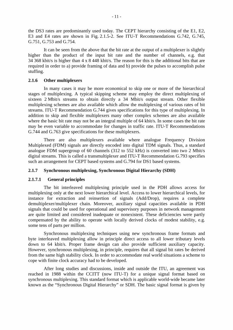
the DS3 rates are predominantly used today. The CEPT hierarchy consisting of the E1, E2, E3 and E4 rates are shown in Fig. 2.1.5-2. See ITU-T Recommendations G.742, G.745, G.751, G.753 and G.754.

It can be seen from the above that the bit rate at the output of a multiplexer is slightly higher than the product of the input bit rate and the number of channels, e.g. that 34 368 kbit/s is higher than 4 x 8 448 kbit/s. The reason for this is the additional bits that are required in order to a) provide framing of data and b) provide the pulses to accomplish pulse stuffing.

2.1.6 Other multiplexers

In many cases it may be more economical to skip one or more of the hierarchical stages of multiplexing. A typical skipping scheme may employ the direct multiplexing of sixteen 2 Mbit/s streams to obtain directly a 34 Mbit/s output stream. Other flexible multiplexing schemes are also available which allow the multiplexing of various rates of bit streams. ITU-T Recommendation G.744 gives specifications for this type of multiplexing. In addition to skip and flexible multiplexers many other complex schemes are also available where the basic bit rate may not be an integral multiple of 64 kbit/s. In some cases the bit rate may be even variable to accommodate for changes in traffic rate. ITU-T Recommendations G.744 and G.763 give specifications for these multiplexers.

There are also multiplexers available where analogue Frequency Division Multiplexed (FDM) signals are directly encoded into digital TDM signals. Thus, a standard analogue FDM supergroup of 60 channels (312 to 552 kHz) is converted into two 2 Mbit/s digital streams. This is called a transmultiplexer and ITU-T Recommendation G.793 specifies such an arrangement for CEPT based systems and G.794 for DS1 based systems.

2.1.7 Synchronous multiplexing, Synchronous Digital Hierarchy (SDH)

2.1.7.1 General principles

The bit interleaved multiplexing principle used in the PDH allows access for multiplexing only at the next lower hierarchical level. Access to lower hierarchical levels, for instance for extraction and reinsertion of signals (Add/Drop), requires a complete demultiplexer/multiplexer chain. Moreover, auxiliary signal capacities available in PDH signals that could be used for operational and supervisory purposes in network management are quite limited and considered inadequate or nonexistent. These deficiencies were partly compensated by the ability to operate with locally derived clocks of modest stability, e.g. some tens of parts per million.

Synchronous multiplexing techniques using new synchronous frame formats and byte interleaved multiplexing allow in principle direct access to all lower tributary levels down to 64 kbit/s. Proper frame design can also provide sufficient auxiliary capacity. However, synchronous multiplexing, in principle, requires that all signal bit rates be derived from the same high stability clock. In order to accommodate real world situations a scheme to cope with finite clock accuracy had to be developed.

After long studies and discussions, inside and outside the ITU, an agreement was reached in 1988 within the CCITT (now ITU-T) for a unique signal format based on synchronous multiplexing. This standard format which is applicable world-wide became later known as the “Synchronous Digital Hierarchy” or SDH. The basic signal format is given by

- 12 -

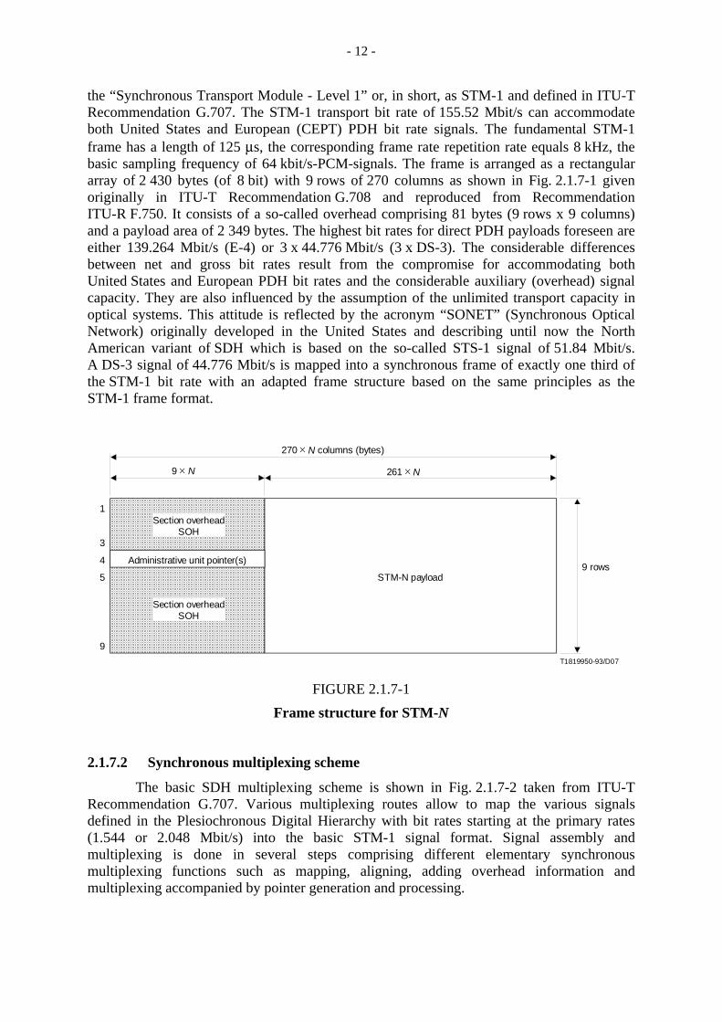
the “Synchronous Transport Module - Level 1” or, in short, as STM-1 and defined in ITU-T Recommendation G.707. The STM-1 transport bit rate of 155.52 Mbit/s can accommodate both United States and European (CEPT) PDH bit rate signals. The fundamental STM-1 frame has a length of 125 µs, the corresponding frame rate repetition rate equals 8 kHz, the basic sampling frequency of 64 kbit/s-PCM-signals. The frame is arranged as a rectangular array of 2 430 bytes (of 8 bit) with 9 rows of 270 columns as shown in Fig. 2.1.7-1 given originally in ITU-T Recommendation G.708 and reproduced from Recommendation ITU-R F.750. It consists of a so-called overhead comprising 81 bytes (9 rows x 9 columns) and a payload area of 2 349 bytes. The highest bit rates for direct PDH payloads foreseen are either 139.264 Mbit/s (E-4) or 3 x 44.776 Mbit/s (3 x DS-3). The considerable differences between net and gross bit rates result from the compromise for accommodating both United States and European PDH bit rates and the considerable auxiliary (overhead) signal capacity. They are also influenced by the assumption of the unlimited transport capacity in optical systems. This attitude is reflected by the acronym “SONET” (Synchronous Optical Network) originally developed in the United States and describing until now the North American variant of SDH which is based on the so-called STS-1 signal of 51.84 Mbit/s. A DS-3 signal of 44.776 Mbit/s is mapped into a synchronous frame of exactly one third of the STM-1 bit rate with an adapted frame structure based on the same principles as the STM-1 frame format.

T1819950-93/D07

4

3

1

9

5

270 × N columns (bytes)

9 × N 261 × N

STM-N payload9 rows

Section overheadSOH

Section overheadSOH

Administrative unit pointer(s)

FIGURE 2.1.7-1

Frame structure for STM-N

2.1.7.2 Synchronous multiplexing scheme

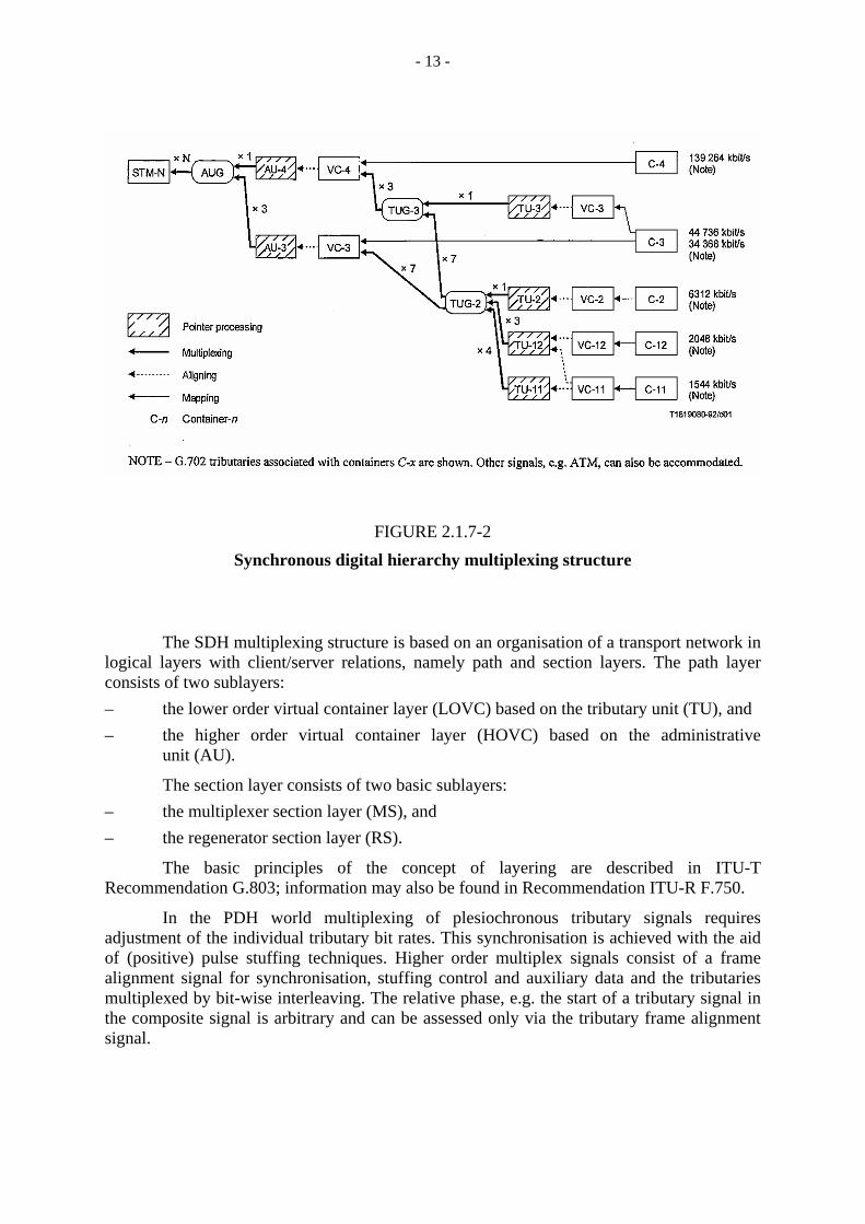
The basic SDH multiplexing scheme is shown in Fig. 2.1.7-2 taken from ITU-T Recommendation G.707. Various multiplexing routes allow to map the various signals defined in the Plesiochronous Digital Hierarchy with bit rates starting at the primary rates (1.544 or 2.048 Mbit/s) into the basic STM-1 signal format. Signal assembly and multiplexing is done in several steps comprising different elementary synchronous multiplexing functions such as mapping, aligning, adding overhead information and multiplexing accompanied by pointer generation and processing.

- 13 -

FIGURE 2.1.7-2

Synchronous digital hierarchy multiplexing structure

The SDH multiplexing structure is based on an organisation of a transport network in logical layers with client/server relations, namely path and section layers. The path layer consists of two sublayers: – the lower order virtual container layer (LOVC) based on the tributary unit (TU), and – the higher order virtual container layer (HOVC) based on the administrative

unit (AU).

The section layer consists of two basic sublayers: – the multiplexer section layer (MS), and – the regenerator section layer (RS).

The basic principles of the concept of layering are described in ITU-T Recommendation G.803; information may also be found in Recommendation ITU-R F.750.

In the PDH world multiplexing of plesiochronous tributary signals requires adjustment of the individual tributary bit rates. This synchronisation is achieved with the aid of (positive) pulse stuffing techniques. Higher order multiplex signals consist of a frame alignment signal for synchronisation, stuffing control and auxiliary data and the tributaries multiplexed by bit-wise interleaving. The relative phase, e.g. the start of a tributary signal in the composite signal is arbitrary and can be assessed only via the tributary frame alignment signal.

- 14 -

For signal synchronization and tributary multiplexing in the SDH, pointer techniques are used in addition to pulse stuffing. Pointer techniques allow to identify the start or relative phase of each tributary signal in an SDH composite signal and can also cope with small rate variations among (quasi) synchronous signals.

The fundamental transformation of plesiochronous signals and rates (with tolerances from 50 to 15 ppm, depending on hierarchical level) to the synchronous domain is accomplished by mapping PDH signal into packets called containers (C-n, with n = 1, 2, 3, 4) which have the basic synchronous repetition rate of 8 kHz. For rate adaptation the classical pulse stuffing procedure is used. Virtual containers (VC-n) are formed by the addition of the related path overhead. They are the basic SDH transport entities. Combining VC-ns with pointers representing phase information (e.g. address of signal byte 1) constitutes (lower order) tributary units (TU-n, with n = 1, 2, 3). They can be synchronously multiplexed into tributary unit groups (TUG-n, n = 2, 3). These TUGs again can be assembled to higher order TUG-3s or VC-ns (with n = 3 or 4). After alignment and combined with the corresponding pointers VC-3s or a VC-4 form administrative units (AU-3 or AU-4). Three multiplexed AU-3 or one AU-4 form the administrative unit group (AUG) which constitutes the payload of an STM-1 signal. The addition of the section overhead (SOH) makes the STM-1 signal complete.

The simplest example for the SDH multiplexing method occurs for the transport of a C-4 container (representing a 139.264 Mbit/s signal) in an STM-1 signal; the assembly steps are illustrated in Fig. 2.1.7-3. Figure 2.1.7-4 shows a relatively complicated case with more multiplexing steps, the transport of a C-1 container in an STM-1 module. The individual processing steps and the constituents of the different entities can be clearly seen in both figures which were taken again from ITU-T Recommendation G.707.

To allow flexible and efficient transport in cases where payload bit rates do not fit very well to the hierarchical levels, concatenation of a multiplicity of suitable virtual containers is foreseen. Concatenated VC-ns (VC-n-c) require coordination in signal handling and present quite demanding signal processing requirements.

Higher capacity synchronous signals are assembled by byte wise interleaving of basic STM-1 signals. STM-4, STM-16 and STM-64 signals with bit rates of 622.08 Mbit/s, 2 488.32 Mbit/s and 9 953.28 Mbit/s respectively are now well established. From channel bandwidth constraints an upper limit for the transport capacity of a single digital radio-relay system can be envisaged at the STM-4 level.

When STM-N signals are demultiplexed the order of the multiplexing steps used at the transmit side is reversed. As prerequisites for the depacking of the SDH transport entities correct identification and evaluation of the section overheads, the path overheads and the different pointers is required. The generation processes for these information signals at the transmit (multiplexing) side correspond to termination processes on the receive (or demultiplexing side).

- 15 -

T1819940-93/D06

VC-4

AU-4

AUG

STM-N

Container-4

VC-4

SOH AUG AUG

AU-4 PTR

Container-4VC-4 POH

AU-4 PTR VC-4

Logical association

Physical association

PointerPTR

NOTE – Unshaded areas are phase aligned. Phase alignment between the unshaded and shaded areas is defined by thepointer (PTR) and is indicated by the arrow.

FIGURE 2.1.7-3

Multiplexing method directly from Container C-4 using AU-4

2.1.7.3 Overhead functions

The 81 section overhead bytes of an STM-1 signal represent a significant capacity of 5 184 Mbit/s. From these bytes 34 are for well-defined standardized use. Additional six bytes are foreseen for radio specific usage and the rest is reserved national usage (6 bytes) or for future international standardization (26 bytes). The overhead bytes are structured in three different groups, as can be seen from Fig. 2.1.7-5 taken from ITU-T Recommendation G.707: – regenerator section overhead (RSOH), rows 1 to 3; – administrative unit (AU) pointers, row 4, and – multiplex section overhead (MSOH), rows 5 to 9.

In the overhead we can for instance identify frame alignment bytes (A1, A2), order wire channel bytes (E1, E2), data communication channel bytes (D1 to D12) and regenerator and multiplex section error monitoring bytes (B1 and B2 respectively). More details are given in ITU-T Recommendation G.707 and Recommendation ITU-R F.750.

- 16 -

T1819910-93/D03

VC-1

TU-1

TUG-2

TUG-3

VC-4

AU-4

AUG

STM-N

Container-1

VC-1 POH Container-1

VC-1

VC-1VC-1

TU-1 PTR

TU-1 PTRTU-1 PTR

TUG-2 TUG-2

VC-4 POH TUG-3 TUG-3

AU-4 PTR VC-4

VC-4AU-4 PTR

SOH AUG AUG

Logical association

Physical association

PointerPTR

NOTE – Unshaded areas are phase aligned. Phase alignment between the unshaded and shaded areas is defined by the pointer (PTR) and is indicated by the arrow.

FIGURE 2.1.7-4

Multiplexing method directly from Container C-1 using AU-4

2.1.7.4 The Sub-STM-1 signal format

In many practical network applications full STM-1 transport capability is not required and quite often the bandwidth of radio channels is too small to support full STM-1 transmission. For applications relying on such band limited terrestrial (or satellite) radio channels a (quasi) synchronous signal format with a bit rate significantly below that of an STM-1 signal would be useful. Within the radio standardization community in ITU-R and at ETSI such a signal format was developed and consensus with ITU-T was achieved. It provides one third of the capacity of an STM-1 signal and maintains most of the benefits of synchronous transmission.

- 17 -

9 bytes

A2

E1

D2

K1

D5

D8

D11

Z2

A2

Z2

A2

M1

A1

B2

Z1

A1

B2

Z1

A1

B1

D1

B2

D4

D7

D10

S1

9rows

C1

F1

D3

K2

D6

D9

D12

E2

* *

Administrative Unit pointer(s)

RSOH

MSOH

Bytes reserved for national use

* Unscrambled bytes.Therefore care should be taken with their content

Note: All unmarked bytes are reserved for future

international standardisation (for media dependent,

additional national use and other purposes)

Media dependant bytes

FIGURE 2.1.7-5

Overhead functions for STM-1 signal

This signal format is called Sub STM-1 and has a gross bit rate of 51.84 Mbit/s which happens to be just the rate of the basic North American Sonet signal called STS-1. The maximum transport capacity is equivalent to one VC-3. A modified and amended multiplexing diagram was derived from the basic SDH multiplexing scheme given in Fig. 2.1.7-2. In Fig. 2.1.7-6 this special multiplexing diagram (as given in Annex A of G.707 and also in Recommendation ITU-R F.750) is presented showing the Sub STM-1 radio frame signal and its relations to the other SDH and PDH transport entities.

The Sub STM-1 signal format does, however, not represent an additional Network Node Interface (NNI). There is also no direct multiplexing path between Sub-STM-1 and STM-1. Interconnection to an SDH network is possible only via standard NNIs based on the STM-1 format. The STM-1 interface signals in these cases are considered to be partially filled only, e.g. carrying only one VC-3.

- 18 -

NNI STM-1x1

AUGx1

AU-4 VC-4

x3

x3

x1

AU-3 VC-3 C-3

x7

RRRP STM-RR TUG-2 TU-2 VC-2 C-2

x3

TU-12 VC-12 C-12

x4

TU-11 VC-11 C-11

*44 736 kbit/s34 368 kbit/s

*

6 312 kbit/s

*

2 048 kbit/s

*

1 544 kbit/s

Pointer processing

Multiplexing

Aligning

Mapping

TUG-3 VC-3TU-3

RR-RP

RR-RP: radio-relay reference point for sub-STM-1 radio-relay

* ITU-T Recommendation G.703 tributaries associated with containers C-x recognised by ITU-T Rec. G.707 are shown. Other signals, e.g. ATM, can also be accommodated.

FIGURE 2.1.7-6

Multiplexing scheme for Sub-STM-1 signal format

The structure of the Sub-STM-1 signal is shown in Fig. 2.1.7-7. The overhead foreseen consists of only three columns with a reduced overhead capability. The overhead structure was derived from the STM-1 signal and is very similar to that of the STS-1 signal. The payload area is filled with one VC-3, the corresponding path overhead and three columns of fixed stuff necessary for capacity alignment.

2.1.7.5 ATM transport in the SDH, SDH transport via PDH signals

The STM-N signal formats are not only suitable for the transport of continuous digital signals but may also be used for cell based transport such as required for B-ISDN with ATM (Asynchronous Transfer Mode), a packet transmission system. The details are covered in ITU-T Recommendation I.432.

On the other hand special synchronous PDH frame formats using the well-known PDH bit rates have been defined in ITU-T Recommendation G.832. The frame repetition rate is set to 8 kHz equivalent to a frame length of 125 µs. The signal formats provide some rudimentary overhead capability and can support the transport of SDH transport entities such

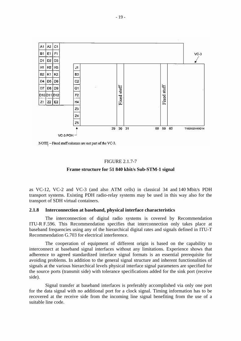
- 19 -

FIGURE 2.1.7-7

Frame structure for 51 840 kbit/s Sub-STM-1 signal

as VC-12, VC-2 and VC-3 (and also ATM cells) in classical 34 and 140 Mbit/s PDH transport systems. Existing PDH radio-relay systems may be used in this way also for the transport of SDH virtual containers.

2.1.8 Interconnection at baseband, physical interface characteristics

The interconnection of digital radio systems is covered by Recommendation ITU-R F.596. This Recommendation specifies that interconnection only takes place at baseband frequencies using any of the hierarchical digital rates and signals defined in ITU-T Recommendation G.703 for electrical interference.

The cooperation of equipment of different origin is based on the capability to interconnect at baseband signal interfaces without any limitations. Experience shows that adherence to agreed standardized interface signal formats is an essential prerequisite for avoiding problems. In addition to the general signal structure and inherent functionalities of signals at the various hierarchical levels physical interface signal parameters are specified for the source ports (transmit side) with tolerance specifications added for the sink port (receive side).

Signal transfer at baseband interfaces is preferably accomplished via only one port for the data signal with no additional port for a clock signal. Timing information has to be recovered at the receive side from the incoming line signal benefiting from the use of a suitable line code.

- 20 -

The primary parameters for baseband interface signals are signal structure and logical format, nominal bit rate and bit rate tolerance. Physical parameters for electrical interfaces contain signal levels, nominal impedances including return loss and type of line coding. Usually asymmetrical interface with a nominal impedance of 75 Ω are used. Line coding is implemented for spectral shaping, to avoid any DC component in the line signal and for ease of clock recovery at the receive end. Prominent ternary and binary line codes are AMI, HDB3, B6ZS and CMI. Signal levels at the transmit side are usually a few volts peak-to-peak. Transmit signals have to meet pulse masks. Signal attenuation up to specified values (6 or 12 dB) must not prohibit correct signal recovery at the receive end. The detailed electrical interface parameters are given in ITU-T Recommendation G.703 for PDH signals and also for the basic SDH STM-1 signal. Digital radio-relay systems could also use an optical interface defined in ITU-T Recommendation G.957.

In addition to the basic interface signal parameters further signal characteristics have to be specified to satisfy network integrity requirements. Examples are performance parameters in general as well as jitter and wander specifications in particular. These are introduced in the next paragraph.

2.1.9 Jitter and wander timing and synchronisation

In extended networks with cascaded clock recovery and multiplex/demultiplex actions signal transport is affected by accumulated signal. These fluctuations have statistical and systematic (quasi-deterministic) components and may be interpreted as phase noise of the clock signals. The slow phase variation (with modulation components well below 1 Hz) are called wander, the faster variations are called jitter. Jitter and wander are usually specified with reference to an idealized high stability reference clock signal, either in the time domain (e.g. as variation of the transitions instants in unit intervals (UI)) or in the modulation frequency domain. They occur in PDH as well as in SDH transport networks. Jitter specifications contain allowed jitter at signal output ports, tolerable jitter at signal input ports and jitter transfer characteristics between input and output ports of single network elements or paths in a network.

In addition to the jitter added in the transmission path by signal regeneration the multiplexing and demultiplexing actions are other sources for jitter and wander. As a consequence of the necessary rate adaptation during multiplexing the flow of tributary signals is disrupted. Continuous tributary baseband signals after demultiplexing are reconstructed from temporary buffered signals and with the aid of smoothing actions based on (not ideally) recovered original clock signals. Careful multiplex signal design can keep systematic jitter within acceptable limits. Additional and highly sophisticated jitter reduction techniques (Dejitteriser) can remove jitter and wander to a large extent but not completely.

Another remedy against jitter and wander is given by synchronizing all clock signal generators in a network, e.g. in multiplexers, to high stability low phase noise reference clock signals and periodically retiming the data signals (see ITU-T Recommendation G.825).

2.2 Fundamentals of terrestrial digital radio-relay systems

Terrestrial digital radio-relay systems (DRRS) use radio waves as an alternative medium to metallic or fibre optic cables for the transport of digital information signals. The large amount of information to be transmitted by these radio systems requires large bandwidths which are only available in the microwave frequency range. This range extends from about 1.5 GHz to above 56 GHz. High capacity radio-relay systems have to be of the

- 21 -

line-of-sight (LOS) type if stable and reliable radio transmission is to be achieved. The predecessors of the digital radio systems were the analogue radio-relay systems that carried FDM and video signals. Analogue radios appeared soon after 1945 and made use of the new microwave technologies that had been developed for radar systems.

Line-of-sight microwave propagation is quasi optical and is helped by the use of highly directional antennas that make it possible to bridge large distances with relatively small transmitter powers. The requirements of low power and large information bandwidth essentially rules out tropospheric or ionospheric scatter systems, a type of radio system which reaches beyond line-of-sight. The line-of-sight requirement limits the path length between two stations, also called the hop length, to the order of about 100 km, with 40 km being typical over flat terrain. Radio-relay systems usually consist of many hops in tandem, with a division between short haul and long haul systems at about 400 km.

Propagation through the atmosphere is normally very stable but occasionally is affected by atmospheric disturbances that will fade, or even enhance the received signal level. One form of disturbance is clear air or multipath fading and another is rain fading. Rain fading, and multipath fading over a narrow bandwidth, are flat with frequency and simply reduce the signal power at the receiving station. At a fade depth equal to the so-called “fade margin” this will cause the digital signal to make errors, for instance at a bit error ratio (BER) of 10-6. Multipath fading is frequency dispersive by nature and will affect the broader digital spectra, with the result that the transmitted pulses become distorted. This, in effect, will reduce the “flat fade margin” just mentioned. Today these phenomena are well understood and they can be effectively counteracted by suitable system and circuit design. This then leads to digital radio-relay systems that meet all the stringent performance (quality) standards set by ITU-R and ITU-T Recommendations.

From the beginning of digital radio in the early 1970s competition with the existing analogue radios required that a certain minimum number of digitized telephone channels be carried by the new digital radio systems. Low-state digital modulation schemes, based on binary or ternary (bipolar) coding used in cable systems, were found to be much too wasteful of frequency space when compared with analogue long haul radios then operating in the 4 and 6 GHz frequency bands. Early systems therefore used 4-state (4-PSK, QPSK, OQPSK, 4-QAM, MSK, TFM) and 8-state (8-PSK) modulation which quickly grew into higher state formats like 16-QAM and 64-QAM, with more recent extensions to 128, 256 or even 512-QAM. The more complex modulations are spectrally very efficient but they require high carrier-to-noise ratios to operate at a given BER. This means that higher transmitter powers are required. They are also more susceptible to degradation from channel impairments. Therefore, where spectrum is relatively plentiful, i.e. in frequency bands above 15 GHz, 4-state modulation schemes like 4-FSK are being used extensively.

With this brief introduction of radio fundamentals the reader is referred to the succeeding chapters for a more detailed description. For instance, we refer to § 4.1 for a detailed explanation of propagation phenomena. Section 4.3 describes the countermeasures used to combat multipath fading. Performance requirements are introduced in § 3.2, and Chapter 5 on Link Engineering describes how radio hops are designed for good performance under fading conditions.

Modulation formats with their bandwidth and carrier-to-noise requirements and their susceptibility to system impairments are described in § 4.2.2.

- 22 -

A discussion of the various digital services carried over radio-relay systems is found in § 3.1 together with information on the available microwave frequency bands. Frequency bands are further subdivided into individual radio channels of various bandwidths, to be found in § 3.4 on RF channel arrangements. The problem of coexistence between digital and analogue radio systems is addressed in § 3.3, microwave interference in § 5.3.5 and sharing between terrestrial and satellite systems in § 3.5.

2.2.1 Architecture of digital radio-relay systems

We now like to introduce digital radio-relay systems through a sequence of block diagrams that describe all the basic functions of the radio equipment. We use as an example a high capacity digital radio system of the long haul and multi channel type. It carries three DS3 bit streams per 30 MHz radio channel, operates in the lower 6 GHz band and uses the 64-QAM modulation format.

We break down the radio equipment into digital transmitters and radio transmitters on the transmitting side and into radio receivers and digital receivers on the receiving side. This break takes place at the 70 MHz IF frequency which is used in this heterodyne radio system. The radio system consists of up to N = 7 regular channels and one protection channel, further arranged into multihop N + 1 switching sections that perform fully automatic protection switching in case of equipment failure or fading. The overall long haul radio system is built up of cascaded switching sections. These basic elements will now be described.

2.2.1.1 Digital transmitter

Figure 2.2.1-1 shows the block diagram of the digital transmitter. According to Recommendation ITU-R F.596 digital radio systems can only be interconnected with other equipment at the well defined hierarchical digital rates. Such an interconnect point is at the input of the transmitter of Fig. 2.2.1-1 and the rate used is the DS3 rate. Disregarding the switches which will be described in § 2.2.1.4, the bipolar DS3 code is first changed into a unipolar format in the DS3 decoder. Three DS3 signals are multiplexed together under a new radio frame that contains stuffing bits and adds about 9 Mbit/s of extra overhead bits to be used for various radio functions. It should be noted that this multiplexing process is strictly internal to the radio system and is not standardized by the ITU-T, with different radio manufacturers employing different multiplexing methods. This has no adverse consequences for the customer because digital radios are sold by switching sections whose inputs and outputs are at the ITU-T standardized hierarchical rates. After this multiplexing operation the effective bit rate over the radio will be about 144 Mbit/s of which 135 Mbit/s are the incoming information bits (which also include framing bits embedded in the DS3 signal). The information bits are transmitted with no change at all, which makes the radio system a clear-channel payload transport facility.

The information bits are further scrambled in a synchronized scrambler which, in contrast to self-synchronized scramblers, avoids any subsequent error multiplication in the descrambler. We note that bit scrambling provides considerable advantages over an unscrambled bit stream. First, the randomized bit sequence assures a smooth emitted spectrum, free of spectral lines that could cause severe co-channel interference into analogue radio channels. Second, it allows simple AC coupling of the bit stream without resorting to the complications of bipolar coding or quantized feedback. Third, it guarantees the necessary spectral components (after suitable signal processing) to facilitate efficient timing and carrier recovery.

FI

GU

RE

2.2

.1-1

Dig

ital

tran

smit

ter

- 23 -

- 24 -

The high bit rate of 144 Mbit/s never directly appears in the radio equipment because the signal is carried on six parallel rails, each with a symbol rate of 24 MBd. Error correction (EC) has been added to modern digital radio systems as a powerful means of reducing bit errors, practically eliminating them at low bit error ratios. The particular EC code used in our example increases the bit rate by 5.5% or about 7.5 Mbit/s. This is a considerably smaller percentage than used in some trellis codes or in codes used for digital mobile radio. The code is an optimal convolutional self-orthogonal code with a rate of 18/19 and the coding gain achieved at a BER = 10-6 is 3 dB (see also § 4.3.5).

Additional bits are added to set up a cyclic redundancy code (CRC) that is able to measure single and double bit errors. This allows isolation of errors to a particular radio hop. The remaining overhead bits form a 384 kbit/s signal providing a total of six 64 kbit/s channels. Four of these channels can be used at the customer's discretion, one is used for order wire and the last one to transmit alarm, status and control information, protection switching signalling, and control signals for Adaptive Transmitter Power Control (ATPC). By adding even more overhead bits it becomes possible to transmit one or two “wayside” channels at the DS1 rate for the customer’s convenience.

Next in the circuit diagram, a D/A converter changes the signal into an 8-level pulse amplitude modulated format on both the in-phase (I) and quadrature (Q) rails that feed the 70 MHz 64-QAM modulator. The Nyquist filter generates a pulse-amplitude spectrum at the modulator input that is equal to the square root of the desired Nyquist spectrum of the received pulses. This assures “matched filter” reception in the receiver. The Nyquist spectrum is often chosen to have a cosine roll-off, in our case with a roll-off factor of 31%. The Nyquist filters shown in Fig. 2.2.1-1 are analogue filters but it is possible to use digital filters, which requires moving the D/A conversion to the filter outputs (see also § 4.2.2).

2.2.1.2 Digital receiver

The digital receiver shown in Fig. 2.2.1-2 coherently demodulates the received 64-QAM signal using a recovered 70 MHz carrier. At the output of the delay equalized Nyquist channel, the baseband pulses are free of intersymbol interference, assuming the radio path is not faded. During periods of multipath fading, however, intersymbol interference can become so severe that useful transmission ceases. By using adaptive transversal equalizers, pulse distortions caused by fading can be considerably reduced. The equalizers are also helpful in mopping up residual linear distortions in the unfaded channel. The block diagram shows a digital transversal equalizer (DTE) which is a modern version of the previously used analogue circuits. The digital form of the baseband input signal is produced by an A/D converter, which may be typically an 8-bit converter, sampling at the symbol rate of 24 MBd.

FI

GU

RE

2.2

.1-2

Dig

ital

rec

eive

r

- 25 -

- 26 -

Internal operation of the DTE is completely binary which includes the decision circuits as well as the decision feedback circuit that generates the various control signals (DTEs use special purpose VLSI devices). The baseband AGC circuit preceding the A/D helps achieve a constant-amplitude eye diagram at the decision circuit.

Advances in integrated circuit technology now make it possible to replace the QAM demodulators and Nyquist filters with their digital equivalents. Since the 70 MHz frequency is too high for the necessary A/D converter in this case, a downconversion to a lower frequency has to take place first.

The DTE may be followed by an adaptive digital linearizer which would replace the analogue IF predistorter normally located in the radio transmitter. Each decision circuit delivers its regenerated 8-level PAM signal (still in binary form) to an A/D converter which generates 24 MBd unipolar pulses appearing on six rails.

Error correction takes place next followed by demultiplexing of the CRC and service channel signals. Finally, the information bits (135 Mbit/s) are demultiplexed, descrambled and put into the DS3 signal format. We note again that the extra 9 Mbit/s overhead bits are only used internally to the radio system and are not passed on to the DS3 interconnect points. Clear-channel operation is therefore guaranteed. The violation monitor restorer (VMR) is used to check the DS3 parity bit and to insert the alarm indication signal (AIS) in case the frame of the DS3 signal is lost. The VMR also restores the parity bit for correct parity, such that the DS3 signal delivered to the network interconnect point looks error-free. This technique allows failure (error) sectionalization in a digital network. To facilitate maintenance, the radio system is connected via a mediation device and a data channel to a remotely located centralized operations system (see also Chapter 6).

Radio repeaters within a switching section regenerate the digital signal. The digital regenerator receives the 64-QAM signal from the 70 MHz output of the radio receiver and delivers it to the 70 MHz input of the radio transmitter (see § 2.2.1.3). Only parts of the circuits shown in Figs. 2.2.1-1 and 2.2.1-2 are required as indicated by arrows REGr and REGt. We note that the regenerator provides access to the service channel and the CRC bits for performance monitoring. The error correction circuits are not used in the regenerator, and access to DS3 is not available.

2.2.1.3 Radio transmitter and receiver

The radio transmitter shown in Fig. 2.2.1-3 follows the conventional heterodyne architecture consisting of upconverter, RF power amplifier and channel combining network. We also show an IF signal attenuator that would be used if adaptive transmitter power control (ATPC) is employed. ATPC is an effective method of reducing microwave interference in a digital network by operating radio transmitters at low power most of the time except during atmospheric fading. ATPC requires a control signal which is derived from the fade depth that is measured in the succeeding radio receiver and sent back to the preceding station transmitter (see also § 4.2.3 , 4.3.4 and 5.3.5.2).

In many applications, GaAsFET amplifiers with linear output powers of several watts will meet system performance requirements. In more demanding cases a Travelling Wave Tube (TWT) with about 10 W output power may be needed. Today, TWTs are the only vacuum tubes still encountered in radio-relay systems. The saturation power of these amplifiers is substantially higher than the linear operating power since adequate linearity can

FIG

UR

E 2

.2.1

-3

Rad

io tr

ansm

itte

r

- 27 -

- 28 -

only be achieved with “backoff” from saturation power. Since backoff is an expensive solution a linearizer circuit, also called a predistorter, is sometimes inserted on the IF side of the radio transmitter. A predistorter is an expanding nonlinear device that is manually adjusted to cancel the compressive nonlinearity of the power amplifier. As a result, backoff can be reduced by several dB. A digital solution to linearization is the adaptive digital linearizer (ADL) circuit previously shown in Fig. 2.2.1-2 (see also § 4.2.3).

Figure 2.2.1-4 shows a radio receiver in a space diversity configuration. Common waveguide low noise GaAsFET preamplifiers are shown in the runs from the receiving antennas (separate transmitting antennas are used in this high capacity digital radio system). The GaAsFET amplifiers cover the full 500 MHz radio band at 6 GHz. Their linearity has to be sufficient in order to keep the intermodulation products generated by the received carriers at a low enough level.

Downconverters become somewhat nonlinear when they are hit by large signal levels during upfades. This nonlinear effect is prevented by a variable attenuator preceding the downconverter, operating under AGC control. An image reject mixer is normally used in this case to eliminate noise originating at the image port.

In space diversity applications using IF combining, the LO signals for the two downconverters have to be derived from the same source, often a dielectric resonator oscillator (DRO). The dielectric used is a ceramic material that has a high dielectric constant (e.g. 40), very low loss (high Q) and is extremely frequency stable. The IF combiner may consist of a hitless soft switch (see also § 4.3.6).

The rest of the receiver requires little explanation except for the adaptive amplitude slope equalizer (AASE). This type of equalizer was first introduced in the late 1970s after it was determined that linear amplitude distortion caused by multipath fading was the major contributor to outage in a digital radio system, even more so than linear delay or other distortions (see also § 4.2.4).

2.2.1.4 Channel combining and antenna considerations

Channel combining networks are used to connect several transmitters, working on separate channel frequencies, to a single antenna. The same networks are also used to combine receivers. Today, these networks consist of a cascade of circulators and multisection bandpass filters (BPF), see Figs. 2.2.1-3 and 2.2.1-4. The BPFs are waveguide filters at 4 GHz and higher frequency bands, and sometimes use ceramic disks for the individual resonator elements.

On high capacity radio routes where all the available channels in a band are occupied, separate transmitting and receiving antennas have to be used in order to reduce harmful interferences between transmitters and receivers. If only a limited number of channels are equipped it becomes possible to connect transmitters and receivers to the same antenna through a circulator. This duplex operation still requires that full attention be given to the correct selection of transmitter and receiver frequencies in order to avoid third order intermodulation problems. Intermodulation products of the 2A-B and A+B-C type will be generated by transmitter frequencies A, B and C in the incidental nonlinearities found in the common circulator, the waveguide or coaxial cable run, the flanges or connectors, and the antenna. Receivers should avoid the intermodulation frequencies because their threshold may

- 29 -

be degraded. If this is not possible, tests should be performed to assure that the loss of receiver threshold (fade margin) is acceptable.

Antennas are typically of the parabolic dish type. The high performance versions are shrouded by a circular cylinder, which results in a marked decrease in sidelobe level. Antenna diameters of 3 m are often employed in long haul radio systems. More sophisticated antennas like horn reflectors are also used in cases where several frequency bands (e.g. 4, 6 and 10 GHz) and two polarizations (V and H) have to be handled simultaneously. Dominant mode waveguides are normally used to feed tower mounted antennas. Horn reflector antennas have the advantage that they can be fed with large diameter (overmoded) circular waveguide that has very low loss, but care has to be taken to transmit only the dominant mode. In order to avoid the problem of feeder losses, which can reduce the fade margin significantly, the radio equipment is sometimes moved very close to the antenna itself. This has led to the construction of concrete towers containing elevated equipment rooms, or to mounting the radio equipment in boxes directly behind the antenna.

2.2.1.5 Radio switching section

The radio switching section is shown in Fig. 2.2.1-5. This basic building block of a radio route interconnects with other switching sections of the same or a different manufacturer, at one of the hierarchical digital rates, e.g. the DS3 rate. Automatic protection switching takes place between the end stations of the switching section (consisting of n + 1 radio hops) by using an extra radio channel in a frequency diversity configuration (see also § 4.2.5 and 4.3.9). This protection channel, working on its own frequency, is automatically substituted for a failed, faded or noisy regular channel. In the 6 GHz band a single protection channel is shared by up to N = 7 regular channels. The block diagram of Fig. 2.2.1-5 emphasizes the switches used in the process with their detailed locations shown in Figs. 2.2.1-1 and 2.2.1-2.

Of the two types of switches provided, the line switch handling the radio line rate of 144 Mbit/s actually consists of six parallel switches operating on the 24 MBd rails. The line switches located in the first transmitter and the last receiver of the switching section are operated when the bit error ratio (BER) in the last receiver exceeds 10-6 as determined by the error correction circuit. Since the receiving line switch is located after the point where error correction takes place, a practically error-free channel (the BER has been reduced to about 10-11 by EC) will be switched over to the (error-free) protection channel. The process of switching itself also has been made error-free by automatically aligning in time and phase the two bit streams that were earlier bridged by the line switch in the first transmitter of the switching section. The line switch is of particular benefit in counteracting the relatively frequent atmospheric fading events. Since fading progresses slowly compared to the switch operating time, a switch is normally completed without making any errors. This errorless feature is also preserved when switches are used for maintenance activities.

The second type of switches are the equipment switches which operate on the three DS3 tributaries in parallel. The switch is initiated from the VMRs, where DS3 parity bits and frame losses are checked. The equipment switches, which normally use small mechanical devices, protect all the equipment located between the DS3 interconnect points and the line switches. Operation of the equipment switch occurs very infrequently because equipment failures are rare.

FIG

UR

E 2

.2.1

-4

Rad

io r

ecei

ver

- 30 -

FIG

UR

E 2

.2.1

-5

Dig

ital

rad

io s

wit

chin

g se

ctio

n

- 31 -

- 32 -

REFERENCES TO CHAPTERS 1 AND 2

ITU-R Recommendations:

Rec. ITU-R F.596 Interconnection of digital radio-relay systems.

Rec. ITU-R F.750 Architectures and functional aspects of radio-relay systems for SDH-based networks.

Rec. ITU-R F.1092 Error performance objectives for constant bit rate digital path at or above the primary rate carried by digital radio-relay systems which may form part of the international portion of a 27 500 km hypothetical reference path.

Rec. ITU-R F.1189 Error-performance objectives for constant bit rate digital paths at or above the primary rate carried by digital radio-relay systems which may form part or all of the national portion of a 27 500 km hypothetical reference path

ITU-T Recommendations:

ITU-T Rec. G.702 Digital hierarchy bit rates.

ITU-T Rec. G.703 Physical/electrical characteristics of hierarchical digital interfaces.

ITU-T Rec. G.707 Synchronous digital hierarchy bit rates.

ITU-T Rec. G.708 Network node interface for the synchronous digital hierarchy.

ITU-T Rec. G.711 Pulse code modulation (PCM) of voice frequencies.

ITU-T Rec. G.732 Characteristics of primary PCM multiplex equipment operating at 2 048 kbit/s.

ITU-T Rec. G.736 Characteristics of primary PCM multiplex equipment operating at 2 048 kbit/s and offering synchronous digital access at 384 kbit/s and/or 64 kbit/s.

ITU-T Rec. G.742 Second order digital multiplex equipment operating at 8 448 kbit/s and using positive justification.

ITU-T Rec. G.744 Second order PCM multiplex equipment operating at 8 448 kbit/s.

ITU-T Rec. G.745 Second order digital multiplex equipment operating at 8 448 kbit/s and using positive/zero/negative justification.

ITU-T Rec. G.751 Digital multiplex equipments operating at the third order bit rate of 34 368 kbit/s and the fourth order bit rate of 139 264 kbit/s and using positive justification.

ITU-T Rec. G.753 Third order digital multiplex equipment operating at 34 368 kbit/s and using positive/zero/negative justification.

- 33 -

ITU-T Rec. G.754 Fourth order digital multiplex equipment operating at 139 264 kbit/s and using positive/zero/negative justification.

ITU-T Rec. G.763 Digital circuit multiplication equipment using ADPCM (Recommendation G.726) and digital speech interpolation.

ITU-T Rec. G.793 Characteristics of 60-channel transmultiplexing equipments.

ITU-T Rec. G.803 Architectures of transport networks based on the synchronous digital hierarchy (SDH).

ITU-T Rec. G.825 The control of jitter and wander within digital networks which are based on the synchronous digital hierarchy (SDH).

ITU-T Rec. G.826 Error performance parameters and objectives for international, constant bit rate digital paths at or above the primary rate.

ITU-T Rec. G.832 Transport of SDH elements on PDH networks - Frame and multiplexing structures.

ITU-T Rec. G.957 Optical interfaces for equipments and systems relating to the synchronous digital hierarchy.

ITU-T Rec. H.120 Codecs for videoconferencing using primary digital group transmission.

ITU-T Rec. H.130 Frame structures for use in the international interconnection of digital codecs for videoconferencing or visual telephony.

- 34 -

CHAPTER 3

LINK DESIGN CONSIDERATIONS

3.1 Applications of digital radio-relay systems

3.1.1 General

Digital radio-relay systems (DRRS) are used in many applications ranging from transporting telephone and TV signals to carrying a wide variety of modern data signals. Distances bridged may range from less than a kilometre to a continent or beyond. Similarly, the capacity of a digital radio system may be as little as a single DS1 signal (1.54 Mbit/s) or as large as 1 000 Mbit/s. Only a small range of the electromagnetic spectrum is suitable for radio-relay applications and within this range only a limited number of bands are available. The bands are further subdivided into channels that can carry either low capacity or high capacity digital signals.

The growth of digital networks was dictated for more than thirty years by the conversion of voice telephone traffic from analogue to digital. Not until recently has pure data traffic been an important factor. Data traffic is now increasingly generated by voice band modems, ISDN terminals, video conferencing and high quality television terminals and other data sources.

The process of digitizing the analogue voice channel started in the United States of America in the early 1960s with the T1 carrier system (using the DS1 signal) that used existing twisted pair cables 24 times more efficiently than analogue circuits. The digital transmission was not only found to be cheap but it provided consistently high quality and required little maintenance. The T1 system found an enormous application in interoffice and toll connecting trunks located mostly in urban areas. With the introduction of digital toll switches (4-ESS) in the mid 1970s, also working at the DS1 rate, growth became even greater. Long haul systems on the other hand remained stubbornly analogue for many years because of low analogue transmission costs. This changed only in the early 1980s with the introduction of cost effective high capacity digital radio systems and later the deployment of optical fibre cables.

The advantages of digital radio-relay systems include:

– Low costs: Radio is cost-effective in comparison with other alternative systems like copper and fibre optic cable. The installation of cable and the cable itself can be very expensive and in urban areas it may be difficult to acquire the necessary rights-of-way.

– Rapid deployment: Radio equipment can be easily moved to new sites to meet rapidly evolving network requirements. Infrastructure requirements are small.

– Ease of maintenance: Maintenance is limited to the infrequent radio stations along the radio path in contrast to cable system where the entire path is exposed to potential cable breaks.

- 35 -

3.1.2 Available frequency bands

The ITU conducts periodic international conferences, the World Radiocommunication Conferences or WRCs, where the electromagnetic spectrum is allocated to various users. Regional Radiocommunication Conferences (RRCs) are also held to develop agreements covering the use of the RF spectrum at the regional level. The results are published in the Radio Regulations as the ITU Table of Frequency Allocations which covers the spectrum from 9 kHz to 400 GHz. In addition to the fixed terrestrial and fixed-satellite services of concern here the spectrum is allocated to many other users like mobile (land, aeronautical, maritime), broadcast, (sound, TV) meteorological, space (operation, research, inter-satellites Earth exploration) radio astronomy, amateur and radiodetermination (radar). The Radio Regulations (RR) allocate the spectrum in only the broadest possible terms.

Most of the countries use the RR as the basis for their own national frequency tables in which they provide additional details, segregated into government and non-government usage.

The frequency tables so far mentioned are only of very general interest to the radio link designer. Over a period of many years the CCIR, now ITU-R, has developed Recommendations on how the available frequency bands should be channelized for analogue and digital radio applications. Radiocommunication Study Group 9 has issued Recommendations and Reports that are contained in its publications under the heading: Section 9B (Radio frequency channel arrangements, spectrum utilization interconnection and maintenance). A very useful list of all the issued Recommendations is contained in Tables 1 and 2 of Recommendation ITU-R F.746 which are reproduced here as Tables 3.1.2-1 and 3.1.2-2. The column labelled “channel spacing” gives a good idea about the digital capacity that can be carried by an individual channel. For details about the channelization plans the reader has to consult the specific Recommendation. An in-depth discussion of the principles underlying the ITU-R recommended channel arrangements is given in § 3.4.

The ITU-R Recommendations may not always reflect the latest channel arrangements used in individual countries. New channel initiatives often start in a particular country and are recognized only some time later in an ITU-R Recommendation. If a manufacturer plans to supply radio equipment into a foreign market it is therefore necessary to become familiar with that country's particular developments. A country may also allow a non-standard channel arrangement or open up a government frequency band to non-government use. Furthermore, in some countries spectrum may be sold by auction with the successful bidder allowed to use it rather freely.

In many countries the distinction between frequencies used by “the telephone company” (also called common carrier or telephone administration) and other private telecommunications enterprises is disappearing. This means that frequency bands that in the past were exclusively reserved for one or the other type of user will be opened up to both.

- 36 -

TABLE 3.1.2-1

Radio frequency channel arrangements for radio-relay systems in frequency bands below about 17 GHz

Band Frequency range Rec. ITU-R Channel spacing (GHz) (GHz) F-Series (MHz)

1.4 1.35-1.53 Rec.[Doc. 9/12] 0.25; 0.5; 1; 2; 3.5

2 1.427-2.69 701 0.5 (pattern) 1.7-2.1; 1.9-2.3 382 29 1.7-2.3 283 14 1.9-2.3 1098 3.5; 2.5 (patterns) 1.9-2.3 1098, Annexes 1 and 2 14 1.9-2.3 1098, Annex 3 10 2.3-2.5 746, Annex 1 1; 2; 4; 14; 28 2.29-2.26 Rec.[Doc. 9/13] 0.25; 0.5; 1; 1.75; 2; 3.5;

7; 14; 2.5 (pattern) 2.5-2.7 283 14

4 3.8-4.2 382 29 3.6-4.2 635 10 (pattern) 3.6-4.2 635, Annex 1 90; 80; 60; 40

5 4.4-5.0 746, Annex 2 28 4.4-5.0 1099 10 (pattern) 4.4-5.0 1099, Annex 1 40; 60; 80 4.54-4.9 1099, Annex 2 40; 20

L6 5.925-6.425 383 29.65 5.85-6.425 383, Annex 1 90; 80; 60

U6 6.425-7.11 384 40; 20 6.425-7.11 384, Annex 1 80

7 7.425-7.725 385 7 7.425-7.725 385, Annex 1 28 7.435-7.75 385, Annex 2 5 7.11-7.75 385, Annex 3 28

8 8.2-8.5 386 11.662 7.725-8.275 386, Annex 1 29.65 7.725-8.275 386, Annex 2 40.74 8.275-8.5 386, Annex 3 14; 7

10 10.3-10.68 746, Annex 3 20; 5; 2 10.5-10.68 747, Annex 1 7; 3.5 (patterns) 10.55-10.68 747, Annex 2 5; 2.5; 1.25 (pattern)

11 10.7-11.7 387, Annex 1 and 2 40 10.7-11.7 387, Annex 3 67 10.7-11.7 387, Annex 4 60 10.7-11.7 387, Annex 5 80

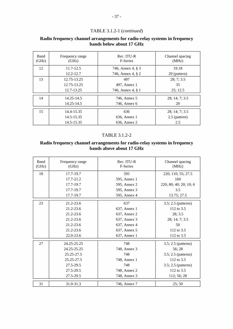
- 37 -

TABLE 3.1.2-1 (continued)

Radio frequency channel arrangements for radio-relay systems in frequency bands below about 17 GHz


12 11.7-12.5 746, Annex 4, § 3 19.18 12.2-12.7 746, Annex 4, § 2 20 (pattern)

13 12.75-13.25 497 28; 7; 3.5 12.75-13.25 497, Annex 1 35 12.7-13.25 746, Annex 4, § 1 25; 12.5

14 14.25-14.5 746, Annex 5 28; 14; 7; 3.5 14.25-14.5 746, Annex 6 20

15 14.4-15.35 636 28; 14; 7; 3.5 14.5-15.35 636, Annex 1 2.5 (pattern) 14.5-15.35 636, Annex 2 2.5

TABLE 3.1.2-2

Radio frequency channel arrangements for radio-relay systems in frequency bands above about 17 GHz


18 17.7-19.7 595 220; 110; 55; 27.5 17.7-21.2 595, Annex 1 160 17.7-19.7 595, Annex 2 220; 80; 40; 20; 10; 6 17.7-19.7 595, Annex 3 3.5 17.7-19.7 595, Annex 4 13.75; 27.5

23 21.2-23.6 637 3.5; 2.5 (patterns) 21.2-23.6 637, Annex 1 112 to 3.5 21.2-23.6 637, Annex 2 28; 3.5 21.2-23.6 637, Annex 3 28; 14; 7; 3.5 21.2-23.6 637, Annex 4 50 21.2-23.6 637, Annex 5 112 to 3.5 22.0-23.6 637, Annex 1 112 to 3.5

27 24.25-25.25 748 3.5; 2.5 (patterns) 24.25-25.25 748, Annex 3 56; 28 25.25-27.5 748 3.5; 2.5 (patterns) 25.25-27.5 748, Annex 1 112 to 3.5 27.5-29.5 748 3.5; 2.5 (patterns) 27.5-29.5 748, Annex 2 112 to 3.5 27.5-29.5 748, Annex 3 112; 56; 28

31 31.0-31.3 746, Annex 7 25; 50

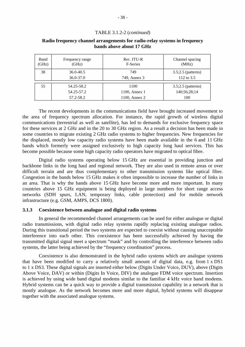
- 38 -

TABLE 3.1.2-2 (continued)

Radio frequency channel arrangements for radio-relay systems in frequency bands above about 17 GHz


38 36.0-40.5 749 3.5;2.5 (patterns) 36.0-37.0 749, Annex 3 112 to 3.5

55 54.25-58.2 1100 3.5;2.5 (patterns) 54.25-57.2 1100, Annex 1 140;56;28;14 57.2-58.2 1100, Annex 2 100

The recent developments in the communications field have brought increased movement to the area of frequency spectrum allocation. For instance, the rapid growth of wireless digital communications (terrestrial as well as satellite), has led to demands for exclusive frequency space for these services at 2 GHz and in the 20 to 30 GHz region. As a result a decision has been made in some countries to migrate existing 2 GHz radio systems to higher frequencies. New frequencies for the displaced, mostly low capacity radio systems have been made available in the 6 and 11 GHz bands which formerly were assigned exclusively to high capacity long haul services. This has become possible because some high capacity radio operators have migrated to optical fibre.

Digital radio systems operating below 15 GHz are essential in providing junction and backbone links in the long haul and regional network. They are also used in remote areas or over difficult terrain and are thus complementary to other transmission systems like optical fibre. Congestion in the bands below 15 GHz makes it often impossible to increase the number of links in an area. That is why the bands above 15 GHz have become more and more important. In many countries above 15 GHz equipment is being deployed in large numbers for short range access networks (SDH spurs, LAN, temporary links, cable protection) and for mobile network infrastructure (e.g. GSM, AMPS, DCS 1800).

3.1.3 Coexistence between analogue and digital radio systems

In general the recommended channel arrangements can be used for either analogue or digital radio transmissions, with digital radio relay systems rapidly replacing existing analogue radios. During this transitional period the two systems are expected to coexist without causing unacceptable interference into each other. This coexistence has been successfully achieved by having the transmitted digital signal meet a spectrum “mask” and by controlling the interference between radio systems, the latter being achieved by the “frequency coordination” process.

Coexistence is also demonstrated in the hybrid radio systems which are analogue systems that have been modified to carry a relatively small amount of digital data, e.g. from 1 x DS1 to 1 x DS3. These digital signals are inserted either below (Digits Under Voice, DUV), above (Digits Above Voice, DAV) or within (Digits In Voice, DIV) the analogue FDM voice spectrum. Insertion is achieved by using wide band digital modems similar to the familiar 4 kHz voice band modems. Hybrid systems can be a quick way to provide a digital transmission capability in a network that is mostly analogue. As the network becomes more and more digital, hybrid systems will disappear together with the associated analogue systems.

- 39 -

Since analogue radio systems contain many circuits that are also suitable for digital transmission a field retrofit of existing analogue with full scale digital radios has also taken place. In the simplest case this has been achieved by substituting a four level digital signal for the FDM baseband spectrum in an analogue FM radio, resulting in a 4-FSK digital radio relay system. With some extra care these digital channels can even be operated in the same protection switching system together with the unchanged analogue channels. More complex retrofits of analogue radios with 64-QAM digital radios have also been made. Although reusing a large installed analogue base can be cost effective the modern approach is to use digital radio equipment especially developed and optimized for digital transmission.

The problems encountered in upgrading from existing analogue to the new digital radio systems are addressed in more detail in § 3.3.

3.1.4 Digital channel capacity

The bit rates carried by digital radio-relay systems are the rates standardized in ITU-T Recommendations G.702, G.703 and G.704 for the plesiochronous digital hierarchies and in ITU-T Recommendations G.707, G.708 and G.709 for the synchronous digital hierarchies (SDH or SONET). Bit rates fb include multiples of DS1 (1.544 Mbit/s) and DS3 (44.736 Mbit/s), E1 (2.048 Mbit/s) and E3 (34.368 Mbit/s), STS1 or Sub-STM1 (51.84 Mbit/s) and STM-1 (155.52 Mbit/s). These are the bit rates delivered to and from the digital radio. Inside the digital radio system the bit rate fbr is often about 6% higher (fbr = 1.06 fb) because of the addition of forward error correction (FEC) and the addition of extra overhead bits for internal radio maintenance and to achieve the radio-internal multiplexing of several standard bit streams.

In order to be able to compete with the existing analogue radio systems which are spectrally very efficient, the simple bipolar bit streams delivered to the radio have to be modulated on a carrier (normally at IF) in a multistate configuration. This reduces the bandwidth requirements of the digital radio or, for a given bandwidth, increases the bit rate transmitted. A popular modulation scheme is Quadrature Amplitude Modulation (s-QAM), where s is the number of states in the 2-dimensional state (phase) plane. Assuming a Nyquist pulse with cosine roll off factor α (0< α<1) we obtain for the width of the signal spectrum:

BRF = fbr (1 + α) / log2 s = 1.06 fb(1 + α) / log2 s (3.1.4-1)

This number is normally made equal to one of the standardized bandwidths given in the ITU-R Recommendations listed in Tables 3.1.2-1 and 3.1.2-2 by making an initial adjustment of the factor α. The final adjustment of α is made such that the digital spectrum fits under the appropriate emission mask prescribed by one of the standards organizations (e.g. United States Federal Communications Commission (FCC), European Telecommunications Standards Institute (ETSI)).

Equation (3.1.4-1) has been used to generate Table 3.1.4-1 which gives the digital channel capacities in standard ITU rates for various channel bandwidths and modulation schemes.

- 40 -

TABLE 3.1.4-1

Channel capacity of digital radio-relay systems

Channel bandwidth

Capacity (roll-off factor α)

0.2 ⟨ α ⟨ 1

BRF (MHz) 4-QAM

(QPSK,MSK, 4-FSK)

s = 4

16-QAM

s = 16

64-QAM

s = 64

256-QAM

s = 256

512-QAM

s = 512

2.5 2DS1 (0.53) 4DS1 (0.53) 6DS1 (0.53) 10DS1 (0.22) 10DS1 (0.37)

5 4DS1 (0.53) 8DS1 (0.53) 12DS1 (0.53) 20DS1 (0.22) 20DS1 (0.37)

10 8DS1 (0.53) 16DS1 0.53) 1DS3 (0.27) 1DS3 (0.69) 1STS1 (0.46)

1DS3 (0.90) 1STS (0.64)

20 16DS1 (0.53) 1DS3 (0.69) 2DS3 (0.27)1STS1 (1.0)

2DS3 (0.69) 2STS1 (0.46)

3DS3 (0.27)2STS1 (0.64)

40 1DS3 (0.69) 2DS3 (0.69)

2STS1 (0.46) 4DS3 (0.27)3STS1 (0.46)1STM1 (0.46)

5DS3 (0.35) 4STS1 (0.46) 1STM1 (0.94)

6DS3 (0.27)5STS1 (0.31)1STM1 (1.0)

3.5 2E1 (0.61) 4E1 (0.61) 8E1 (0.21) 8E1 (0.61) 12E1 (0.21)

7 4E1 (0.61) 8E1 (0.61) 12E1 0.61) 1E3 (0.54) 1E3 (0.73)

14 8E1 (0.61) 1E3 (0.54) 1E3 (1.0) 2E3 (0.54)

1STS1 (1.0) 2E3 (0.73)1STS1 (1.0)

28 1E3 (0.54) 2E3 (0.54)

1STS1 (1.0) 2E3 (0.54)2STS1 (0.53)

5E3 (0.23) 3STS1 (0.36) 1STM1 (0.36)

5E3 (0.38)3STS1 (0.53)1STM1 (0.53)

56 2E3 (0.54)

1STS1 (1.0) 5E3 (0.23)3STS1 (0.36)1STM1 (0.36)

7E3 (0.32)4STS1 (0.53)1STM1 (1.0)

10E3 (0.23) 6STS1 (0.36) 2STM1 (0.36)

10E3 (0.38)7STS1 (0.31)2STM1 (0.53)

We notice that the first 5 rows in the table are for channel bandwidths that are multiples of 2.5 MHz. This applies mostly to the North American hierarchy. The next 5 rows are in multiples of 3.5 MHz , which are bandwidths most often used for the CEPT hierarchy. Modulation methods from 4-QAM to 512-QAM are considered and roll-off factors α are chosen to be larger than 0.2. We then find the largest possible number of digital channels that can be used in the given channel bandwidth, with the constraint that the number of DS1 and E1 signals are either multiples of two or four. We note that single digital radio channels are capable of meeting a wide range of transmission requirements. By operating multiple channels in a n + 1 protection switching configuration the transmission capacity can be further increased by a factor n.

- 41 -

The spectrum efficiency expressed in bits/second per Hertz of bandwidth, or bit/s/Hz, is found from equation (3.1.4-1) to be:

η = fbr / BRF = log2 s / (1 + α) (3.1.4-2)

The efficiency ranges from about 1.25 bit/s/Hz for 4-QAM to about 6 bit/s/Hz for 512-QAM. In the United States of America minimum efficiency requirements for digital radios working in the frequency bands below 15 GHz were established on the basis that they approximately match the number of telephone channels that could be carried by an analogue radio channel occupying the same bandwidth. This leads to modulation methods that have to be either 16-QAM or 64-QAM, resulting in efficiencies ranging from 2.5 to 4.6 bit/s/Hz. It is clear that matching the analogue radio channel loading was also dictated by economic reasons.

Above 15 GHz, where spectrum is more plentiful, the spectrum efficiency requirement was relaxed to be > 1 bit/s/Hz which allows the much simpler 4-QAM or equivalent modulation schemes to be used. For short single or multi hop connections the simple and rugged 4 level FSK modulation (4-FSK) is being extensively employed in the higher frequency bands. 4-FSK, or FSK in general, has a spectrum that is not very well described by equation (3.1.4-1). The spectrum expands rapidly as the FM deviation is increased. For this reason the deviation in an FSK system has to be adjusted to meet the prescribed emission mask. These masks, for radio systems operating above 15 GHz, fall off less rapidly away from the carrier and therefore accommodate FSK spectra very well.

3.1.5 Digital networks

3.1.5.1 Long haul digital radio systems

Long haul, high capacity digital radio systems can be competitive with optical fibre, especially in difficult terrain like mountains, across lakes or rivers and in urban areas with expensive or unavailable rights-of-way or where speed of deployment is important. Also, digital long haul radio systems can re-use a vast system of towers and buildings, previously used by analogue radio systems employed in national backbone telecommunications networks. Channel capacities employed by these systems are the maximum that can be achieved with high-state QAM modulation schemes (see Table 3.1.4-1). A large number of channels may be operated on the same route by using a n + 1 switching system. Because of the long distances involved the lower frequency bands of 4 and 6 GHz have been widely used in many countries.

3.1.5.2 Short haul digital radio systems

Today digital radio systems find a major application in all those cases where cable laying would be difficult, costly and time consuming. Digital radios can be deployed very rapidly, especially if small unobtrusive antennas can be located on existing buildings or towers and distances are relatively short. Equipment operating at frequencies above 15 GHz meet these requirements very well because it is small, rugged and economical. The explosive growth of cellular networks for mobile radio has generated a large market for these millimetre wave radios. They interconnect cell cites with Mobile Switching Centres (MSC) using capacities that are relatively low, ranging from 1-DS1 to 4-DS1 or 1-E1 to 4-E1. Because of the low capacity, protection is sometimes omitted or otherwise provided by automatic hot standby switching. And since hop lengths are often short there is no need for frequency or space diversity protection against multipath fading. Rain attenuation is the overpowering cause of signal outage, which can be kept within ITU requirements by the use of high system gain radios and short hops.

- 42 -

Where larger hop lengths are required, digital radios operating below 15 GHz have to be used. The 2 GHz band was used extensively in the United States of America for low capacity connections by power and gas companies. This band has now been allocated to various PCN uses and the existing radio services can be redeployed in the Lower 6 GHz (L6), Upper 6 GHz (U6) and 11 GHz bands which have been opened up for low capacity digital applications. These bands are not affected by rain fading and therefore provide large distance capabilities. Space and frequency diversity systems are used here as countermeasures for multipath fading with frequency diversity systems normally operated in the form of a n + 1 protection switching system. In the interest of spectrum conservation, the FCC in the United States of America demands that the number n grows to at least 3 within three years after first deployment on a route. This rules out permanent 1 + 1 frequency diversity systems. Other countries may have other rules or no such requirements.

Examples of radio systems and their system parameters are given in the Tables included in Recommendation ITU-R F.758.

3.1.5.3 Digital radio access networks

Access networks may be classified as a very short version of the classical short haul networks, often consisting of only a single radio hop. (“Short haul” has been traditionally defined as connections not exceeding 250 miles or 400 km).

High capacity radios are used for access (spurs) to long haul radio or fibre optic networks where fibre is often found to be too expensive. Another example is a short radio connection that serves as a fibre optic ring closure in difficult terrain. A single high capacity radio channel carrying a STS-1 or STM-1 signal may suffice for these applications and, if the access consists of a single short radio hop, a millimetre wave radio would be very appropriate.

Low capacity access applications, involving up to 4-E1 or 4-DS1, are common in the rapidly evolving mobile cellular networks such as global system for mobile communications (GSM), advanced mobile phone service (AMPS) and digital cellular system, 1 800 MHz, (DCS 1 800). This includes connections between base station controllers (BSC) and mobile switching centres (MSC). In case of microcell or personal communications networks (PCN) the many small base stations, or base transceiver stations (BTS), will be interconnected to BSCs via access radio. These low capacity applications will almost exclusively use frequency bands above 20 GHz.

3.1.6 Radio Local Area Networks (RLAN)

3.1.6.1 General

Today’s computer-based business activity largely depends on communication infrastructure provided by local area networks (LANs). LANs have to be extended in line with the increase of terminal users, and therefore designed to handle bursty traffic in order to efficiently share computer resources. However wired LAN has many constraints in the aspects of cost, maintenance and installation in particular for networks with complicated architecture. In recent days it is well understood by many LAN users that these constraints can be solved by intelligent application of radio techniques.

General advantages that may be provided by RLAN include:

– rapid initial installation of communication infrastructure in users’ premises;

– saving for maintenance cost required for cable networks;

- 43 -

– flexible rearrangement of network configuration associated with office layout changes;

– untethered use of lightweight personal computers.

Reflecting the above situation Radiocommunication Study Group 9 has been studying RLANs since 1990 under the Question adopted specifically for this issue. Much efforts have been made as far as producing a draft Recommendation, which is expected to become a new Recommendation in 1997. This draft Recommendation deals with basic system parameters, interference compatibility and other technical guidance for system designers.

3.1.6.2 Frequency bands

Low capacity RLANs are developed at UHF. However, a wide range of data rates required for various RLAN applications have lead to the exploitation of SHF and EHF bands.

According to the guidance in the draft Recommendation [Doc. 9/14], proposed frequency bands and appropriate data rates for RLANs are given in Table 3.1.6-1

Many of the bands are already used for outdoor fixed services. In this sense interference compatibility has to be studied to meet local frequency sharing criteria. It should also be noted that the use of other frequency bands is not excluded.

TABLE 3.1.6-1

Examples of frequency bands and data rates

Frequency Frequency bands Approximate data rates

UHF (300-3 000 MHz)

900 MHz band 1 900 MHz band 2 400 MHz band

Up to 6 Mbit/s

SHF

(3-30 GHz)

5.2 GHz band 5.7-5.8 GHz band

17.2 GHz band 18.8 GHz band 19.5 GHz band

Up to 50 Mbit/s

EHF (30-300 GHz)

60 GHz

Under study

NOTE 1 – The use of other frequency bands is not excluded.

3.1.6.3 Multiple access and modulation

Studies on suitable schemes for multiple access and modulation for RLANs are now still progressing. Provisional results have been given as shown in Table 3.1.6-2 through the following discussion.

At UHF, since spectrum is becoming an extremely scarce resource, efficient use of spectrum within a limited space (i.e. tolerance of interference) may be an important factor. Direct sequence or frequency hopping CDMA with some form of PSK can be used as it satisfies this requirement.

- 44 -

On the other hand, at higher frequency bands, signalling schemes that are tolerant of phase noise and frequency offsets may be desirable. Also the relative cost increase due to power control or high order diversity system may become a significant factor.

TABLE 3.1.6-2

Multiple access and modulation schemes for RLANs

Frequency Multiple access Modulation

UHF (300-3 000 MHz)

FDMA, TDMA, CDMA (Direct sequence spread

spectrum, frequency hopping)

FSK, QPSK

SHF (3-30 GHz)

FDMA TDMA CDMA

FSK GMSK QPSK

16-QAM

EHF (30-300 GHz

Under study Under study

3.1.6.4 System configuration

Two basic configurations are proposed for RLAN topologies as shown in Fig. 3.1.6-1

FIGURE 3.1.6-1

RLAN topologies

- 45 -

3.1.6.5 Examples of RLANs

Many RLANs have been reported including those already put into service or to be realized in the near future. Table 3.1.6-3 summarizes typical examples of RLANs using frequency bands above 1 GHz and having maximum data rate higher than 1 Mbit/s.

TABLE 3.1.6-3

Examples of RLAN characteristics

Frequency band Modulation and/or access scheme

Data rate (typical)

Application Range(1) (typical)

403-470 MHz 806-869 MHz 946 MHz

4-level FSK 19.2 kbit/s ARDIS(2) subscriber equipment

ARDIS service area

850 MHz (cellular) FSK 14.4 kbit/s 9.6 kbit/s (Fax)

Personal communication via cellular phone

Cellular phone service area

902-928 MHz Frequency hopping (FSK) 64 kbit/s to 500 kbit/s

Point-to-point data link campus and private networks

4 km

Direct sequence 2 Mbit/s 215 kbit/s to 1.0 Mbit/s

Portable LAN Ethernet LANs

250 m 100 to 1 000 m

CDMA/TDMA spread spectrum

1.536 Mbit/s line rate

Personal communication networks

450 to 5 000 m2

Direct sequence with 1.5 MHz frequency channel selection

60 kbit/s Bar-code reading 120 to 210 m

Direct sequence PSK trellis code

5.7 Mbit/s Ethernet LAN (IEEE 802.3)

80 m

2.4 to 2.4835 GHz 2.4 to 2.485 GHz (transceiver to hub) 5.745 to 5.830 GHz (hub to transceiver)

CDMA, direct sequence frequency hopping Direct sequence 16 PSK trellis code

1 Mbit/s (Approx.) 5.7 Mbit/s

– Ethernet LAN (IEEE 802.3)

– 80 m

5.2 GHz GMSK (BT = 0.4)

24 Mbit/s Raw data rate

High performance RLANs (HIPERLANS)

50 m

17.2 GHz Specification in progress Specification in progress

High performance RLANs (HIPERLANS)

Specification in progress

18.8 GHz 19.2 GHz

TDMA-TDD 4-FSK

15 Mbit/s Ethernet LAN 40 m (maximum)

19.5 GHz TDMA-TDD 4-FSK

25 Mbit/s Ethernet LAN 40 m (maximum)

(1) The range of operation of RLAN systems may vary greatly depending on data rate, frequency, RF power, antenna and the propagation environment. (2) ARDIS: advanced radio data information service.

- 46 -

3.2 Performance and availability objectives

The design of digital radio-relay systems is based on the relevant error performance and availability objectives specified by ITU-R and ITU-T. This section provides explanatory information on the basic concepts used in existing ITU-R Recommendations on error performance and availability, and the relationship to the relevant ITU-T Recommendations.

The aim of this section is to introduce the concepts of error performance and availability as preparation for the consideration of error performance prediction in Chapter 5 and performance measurement in Chapter 6.

3.2.1 Hypothetical digital connection, path and section

The ITU-T Recommendation G.801 defines digital transmission network models that are hypothetical entities of a defined length and composition.

A digital HRX (hypothetical reference connection) is a model in which studies relating to overall performance may be conducted, thereby facilitating the formulation of standards and objectives. In order to initiate studies directed at the performance of an ISDN, an all digital 64 kbit/s connection is considered. Since the overall network performance objectives for any performance parameter need to be consistent with user requirements, such objectives, in the main, should relate to a network model which is representative of the very long connection. The HRX 27 500 km length shown in Fig. 3.2-1 (Fig. 1/G.801) serves this purpose.

To facilitate the study of digital transmission impairments (e.g. bit errors, jitter and wander, slip, transmission delay) it is necessary to define network models comprising a combination of different types of transmission elements (e.g. transmission systems, multiplexers, demultiplexers, digital paths, transcoders). Such a model is defined as a hypothetical reference digital link (HRDL). In ITU-R Recommendations the term hypothetical reference digital path (HRDP) is usually used. A length of 2 500 km is considered as a suitable distance for a HRDP. The 2 500 km HRDP for digital radio-relay systems consists of nine digital radio sections, each approximately 280 km in length, which is defined in Recommendation ITU-R F.556.

To accommodate the performance specification of transmission systems a hypothetical reference digital section (HRDS) is used. Such a model is defined in Fig. 4/G.801 for each level in the digital hierarchies defined in ITU-T Recommendation G.702. The input and output ports are the recommended interfaces as given in ITU-T Recommendation G.703 and Recommendation ITU-R F.556 for hierarchical bit rates. The lengths have been chosen to be representative of digital sections likely to be encountered in real operational networks, and are sufficiently long to permit a realistic performance specification for digital radio systems. The model is homogeneous in that it does not include other digital equipments such as multiplexers/demultiplexers. This entity can form a constituent element of a HRDP. The lengths 50 and 280 km are identified for HRDS in ITU-T Recommendation G.921.

ITU-T Recommendation G.102 provides additional information on transmission performance objectives and related Recommendations.

- 47 -

3.2.2 Error performance parameters and objectives

3.2.2.1 Error performance parameters and objectives based on ITU-T Recommendation G.821

HRX, HRDP and HRDS give the base for identification of error performance and availability parameters.

The ITU-T Recommendation G.821 was developed 15 years ago and was the first Recommendation that dealt with error performance of an international digital connection. It established error performance parameters and objectives for 64 kbit/s circuit and had special procedure in its Annex D for recalculating the objectives if measurements were provided at system bit rate (see § 6.2).

Recommendations ITU-R F.594, ITU-R F.634, ITU-R F.696 and ITU-R F.697 were further developed based on this Recommendation.

In the context of error performance of 64 kbit/s circuit-switched connection types and the allocation of performance to the connection elements, an all digital HRX configuration is given in Fig. 3.2-1.

FIGURE 3.2-1

Note 1 – It is not possible to provide a definition of the location of the boundary between the medium and the high grade portions of the HRX. Note 4 to Table 2/G.821 provides further clarification of this point.

Note 2 – LE denotes the “local exchange” or equivalent point.

Error performance should only be evaluated whilst the connection is in the available state.

Error performance parameters are derived from the following events:

– Errored second (ES): it is a 1 s period in which one or more bits are in error.

– Severely errored second (SES): it is a 1 s period which has a bit error ratio ≥ 1.10-3.

Parameters are:

– Errored second ratio (ESR): the ratio of ES to total seconds in available time during a fixed measurement interval;

– severely errored second ratio (SESR): the ratio of SES to total seconds in available time during a fixed measurement interval.

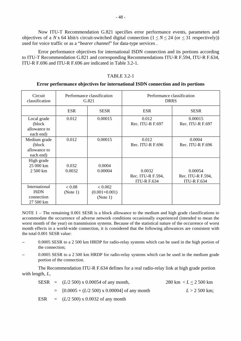
- 48 -

Now ITU-T Recommendation G.821 specifies error performance events, parameters and objectives of a N x 64 kbit/s circuit-switched digital connection (1 < N < 24 (or < 31 respectively)) used for voice traffic or as a “bearer channel” for data-type services .

Error performance objectives for international ISDN connection and its portions according to ITU-T Recommendation G.821 and corresponding Recommendations ITU-R F.594, ITU-R F.634, ITU-R F.696 and ITU-R F.696 are indicated in Table 3.2-1.

TABLE 3.2-1

Error performance objectives for international ISDN connection and its portions

Circuit classification

Performance classification G.821

Performance classification DRRS

ESR SESR ESR SESR

Local grade (block

allowance to each end)

0.012 0.00015 0.012 Rec. ITU-R F.697

0.00015 Rec. ITU-R F.697

Medium grade (block

allowance to each end)

0.012 0.00015 0.012 Rec. ITU-R F.696

0.0004 Rec. ITU-R F.696

High grade 25 000 km 2 500 km

0.032

0.0032

0.0004

0.00004

0.0032 Rec. ITU-R F.594,

ITU-R F.634

0.00054 Rec. ITU-R F.594,

ITU-R F.634 International

ISDN connection 27 500 km

< 0.08 (Note 1)

< 0.002 (0.001+0.001)

(Note 1)

NOTE 1 – The remaining 0.001 SESR is a block allowance to the medium and high grade classifications to accommodate the occurrence of adverse network conditions occasionally experienced (intended to mean the worst month of the year) on transmission systems. Because of the statistical nature of the occurrence of worst month effects in a world-wide connection, it is considered that the following allowances are consistent with the total 0.001 SESR value:

– 0.0005 SESR to a 2 500 km HRDP for radio-relay systems which can be used in the high portion of the connection;

– 0.0005 SESR to a 2 500 km HRDP for radio-relay systems which can be used in the medium grade portion of the connection.

The Recommendation ITU-R F.634 defines for a real radio-relay link at high grade portion with length, L,

SESR = (L/2 500) x 0.00054 of any month, 280 km < L < 2 500 km

= [0.0005 + (L/2 500) x 0.00004] of any month L > 2 500 km;

ESR = (L/2 500) x 0.0032 of any month

- 49 -

3.2.2.2 Error performance parameters and objectives based on ITU-T Recommendation G.826 ITU-T Recommendation G.826 is applicable to international, constant bit rate digital paths at or above the primary rate. These paths may be based on a plesiochronous digital hierarchy, synchronous digital hierarchy or some other transport network such as cell-based. The Recommendation is generic in that it defines the parameters and objectives for paths independent of the physical transport network providing the paths. Compliance with the performance specification of this Recommendation will, in most cases, also ensure that a 64 kbit/s connection will meet the requirements laid out in ITU-T Recommendation G.821. Therefore, G.826 is the only Recommendation required for designing the error performance of transport networks at or above the primary rate.

ITU-T Recommendation G.826 is based upon the error performance measurement of blocks.

A block is a set of consecutive bits associated with the path; each bit belongs to one and only one block. Consecutive bits may not be contiguous in time.

Each block is monitored by means of an inherent error detection code (EDC) (e.g. bit interleaved parity (BIP) or cyclic redundancy code (CRC). The EDC bits are physically separated from the block to which they apply. It is not normally possible to determine whether a block or its controlling EDC bits are in error. If there is a discrepancy between the EDC and its controlled block, it is always assumed that the controlled block is in error.

No specific EDC is given in this generic definition but it is recommended that for in-service monitoring purposes, future designs should be equipped with an EDC capability such that the probability to detect an error event is ≥ 90% assuming Poisson error distribution. CRC-4 and BIP-8 are examples of EDCs currently used which fulfil this requirement.

Estimation of errored blocks on an in-service basis is dependent upon the network fabric employed and the type of EDC available. Annexes to ITU-T Recommendation G.826 offer guidance on how in-service estimates of errored blocks can be obtained from the ISM (in-service measurement) facilities of the PDH.

Error performance parameters are derived from the following events:

– errored block (EB): a block in which one or more bits are in error;

– errored second (ES): a 1 s period with one or more errored blocks or at least one defect;

– severely errored second (SES): a 1 s period which contains ≥ 30 % errored blocks or at least one defect. SES is a subset of ES.

Consecutive severely errored seconds may be precursors to periods of unavailability, especially when there are no restoration/protection procedures in use. Periods of consecutive SES persisting for T s, where 2 < T < 10 (some network operators refer to these events as “failures”), can have a severe impact on service, for example the disconnection of switched services. The only way ITU-T Recommendation G.826 limits the frequency of these events is through the limit for the SES ratio;

– background block error (BBE): an errored block not occurring as part of an SES.

- 50 -

Parameters are:

– errored second ratio (ESR): the ratio of ES to total seconds in available time during a fixed measurement interval;

– severely errored second ratio (SESR): the ratio of SES to total seconds in available time during a fixed measurement interval;

– background block error ratio (BBER): the ratio of BBE to total blocks in available time during a fixed measurement interval. The count of total blocks excludes all blocks during SESs.

Error performance should only be evaluated whilst the path is in the available state.

The ITU-T Recommendation G.826 specifies the end-to-end objectives for a 27 500 km HRDP in terms of the parameters defined above (see Table 3.2-2 (Table 1/G.826)).

An international digital path at or above the primary rate shall meet its allocated objectives for all parameters concurrently. The path fails to meet the error performance requirement if any of these objectives is not met. The evaluation period is 1 month.

TABLE 3.2-2

End-to-end error performance objectives for a 27 500 km international digital HRDP at or above the primary rate

Rate (Mbit/s)

1.5 to 5 >5 to 15 >15 to 55 >55 to 160 >160 to 3500

Bits/block 800-5 000 2 000-8 000 4 000-20 000 6 000-20 000 15 000-30 000 (Note 2)

ESR 0.04 0.05 0.075 0.16 (Note 3)

SESR 0.002 0.002 0.002 0.002 0.002

BBER 2 x 10-4 (Note 1)

2 x 10-4 2 x 10-4 2 x 10-4 10-4

NOTE 1 – For systems designed prior to 1996, the BBER objective is 3 x 10-4.

NOTE 2 – Because bit error ratios are not expected to decrease dramatically as the bit rates of transmission systems increase, the block sizes used in evaluating very high bit rate paths should remain within the range 15 000 to 30 000 bits/block. Preserving a constant block size for very high bit rate paths results in relatively constant BBER and SESR objectives for these paths.

As currently defined, VC-4-4c (ITU-T Recommendation G.707) is a 601 Mbit/s path with a block size of 75 168 bits/block. Since this is outside the recommended range for 160-3 500 Mbit/s paths, performance on VC-4-4c paths should not be estimated in service using this table. The BBER objective for VC-4-4c using the 75 168 bit block size is taken to be 4 x 10-4. There are currently no paths defined for bit rates greater than VC-4-4c (>601 Mbit/s).

- 51 -

Digital sections are defined for higher bit rates and guidance on evaluating the performance of digital sections can be found in § 6.1 and in draft Recommendation ITU-R G.EPMRS.

NOTE 3 – Due to the lack of information on the performance of paths operating above 160 Mbit/s, no ESR objectives are recommended at this time. Nevertheless, ESR processing should be implemented within any error performance measuring devices operating at these rates for maintenance or monitoring purposes. For paths operating at bit rates up to 601 Mbit/s an ESR objective of 0.16 is proposed. This value requires further study.

Digital paths operating at bit rates covered by ITU-T Recommendation G.826 are carried by transmission systems (digital sections) operating at equal or higher bit rates. Such systems must meet their allocations of the end-to-end objectives for the highest bit rate paths which are foreseen to be carried. Meeting the allocated objectives for this highest bit rate path should be sufficient to ensure that all paths through the system are achieving their objective. For example, in SDH, an STM-1 section may carry a VC-4 path and therefore the STM-1 section should be designed such that it will ensure that the objectives as specified in that Recommendation for the bit rate corresponding to a VC-4 path are met.

It is noted that SES events may occur in clusters, not always as isolated events. A sequence of “n” contiguous SES may have a very different impact on performance from “n” isolated SES events.

Objectives are allocated in ITU-T Recommendation G.826 to the national and international portions of a path.

The boundary between the national and international portions is defined to be at an international gateway (IG) which usually corresponds to a cross-connect, a higher-order multiplexer or a switch (N-ISDN or B-ISDN). IGs are always terrestrially based equipment physically resident in the terminating (or intermediate) country. All paths should be engineered to meet their allocated objectives. Network operators should note that if performance could be improved in practical implementations to be superior to allocated objectives, the occurrence of paths exceeding the objectives of Table 3.2-2 can be minimized.

The following apportionment methodology specifies the levels of performance expected from the national and international portions of an HRDP:

a) Allocation to the national portion of the end-to-end path

Each national portion is allocated a fixed block allowance of 17.5% of the end-to-end objective. Furthermore, a distance based allocation is added to the block allowance. The actual route length between the PEP (path end-point) and IG should first be calculated if known. The air-route distance between the PEP and IG should also be used and multiplied by an appropriate routing factor.

b) Allocation to the international portion of the end-to-end path

The international portion is allocated a block allowance of 2% per intermediate country plus 1% for each terminating country. Furthermore, a distance based allocation is added to the block allowance. As the international path may pass through intermediate countries, the actual route length between consecutive IGs (one or two for each intermediate country) should be added to calculate the overall length of the international portion. The air-route distance between consecutive IGs should also be used and multiplied by an appropriate routing factor.

- 52 -

Error performance objectives of ITU-T Recommendation G.826 refer to the hypothetical reference path (HRP) of a length of 27 500 km. ITU-T Recommendation G.826 does not contain information about error performance objectives for path elements.

Now ITU-T is developing draft new Recommendation G. EPMRS which defines error performance events for SDH multiplex sections. SDH equipment functional blocks and SDH management are defined in ITU-T Recommendations G.783 and G.784.

In accordance with ITU-T Recommendation G.826, the events definitions are block-based, making in-service measurement convenient. If required, compliance with this Recommendation may be assessed using out-of-service measurements. This ITU-T Recommendation G.826 is subject to further refinements.

Based on ITU-T Recommendation G.826, ITU-R has developed two new Recommendation for constant bit rate digital path at or above the primary rate carried by digital radio-relay systems which may form part of the international (F.1092) and national (F.1189) portion of a 27 500 km hypothetical reference path accordingly.

Recommendations ITU-R F.1092 and ITU-R F.1189 state that:

– future and, whenever practical, existing digital radio-relay systems at or above the primary rate should comply with error performance objectives aligned to ITU-T Recommendation G 826;

– error performance objectives applicable to radio-relay paths forming part of the international portion of a 27 500 km HRP should be based both on distance-based and on country-based allocations as specified in ITU-T Recommendation G.826;

For national portion the Recommendation ITU-R F.1189 indicates that this portion should consist of three parts:

– long-haul,

– short-haul,

– access,

PEP LE (*) IG

--- --- --- ---

| |-----| |----------| |-----------------| |

--- --- --- ---

Access Short haul Long haul

NOTE (*) – In dependence of the country network architecture, this centre may coincide with a PC, SC or TC (see ITU-T Recommendation G.801).

FIGURE 3.2-2

Basic sections of the national portion of the HRP

- 53 -

where:

– Access : the access network section, including the connections between “path end-point” (PEP) and the corresponding local access switching centre/cross-connector (local exchange (LE));

– Short haul: the short haul inter-exchange network section, including the connections between a local access switching centre/cross-connector (LE) and the “primary centre” (PC), “secondary centre” (SC) or “tertiary centre” (TC) (in dependence of the network architecture);

– Long haul: the long haul inter-exchange network section, including the connections between a PC, SC or TC (in dependence of the network architecture) and the corresponding “international gateway” (IG).

Error performance objectives for DRRS that can form international and national portions of the 27 500 km international digital HRP at or above the primary rate are combined in Table 3.2-3.

TABLE 3.2-3

Error performance objectives for DRRS that can form international and national portions of the 27 500 km international digital HRP at or above

the primary rate up to STM-1

Rate (Mbit/s)

1.5 to 5 (1)

> 5 to 15 > 15 to 55 > 55 to 160

Errored second ratio

0.04 × (FL + BL) 0.05 × (FL + BL) 0.075 × (FL + BL) 0.16 × (FL + BL)

Severely errored seconds ratio 0.002 × (FL + BL)

Background block error ratio 2 × 10–4 × (FL + BL)

(1) For systems designed prior to 1996, the BBER objective is 3x 10-4.

In Table 3.2-3, FL and BL are defined as follows:

a) For international portion

Distance allocation factor (FL) FL = 0.01 x L / 500 L (km) (see Note 1)

Block allowance factor (BL)

– for intermediate countries BL = BR x 0.02 x (L / Lref) for Lmin < L ≤ Lref

BL = BR x 0.02 for Lmin < L > Lref

- 54 -

– for terminating countries BL = BR x 0.01 x (L / Lref) for Lmin < L ≤ Lref

BL = BR x 0.01 for Lmin <L > Lref

Block allowance ratio, (BR) (0 < BR ≤ 1)

Reference length (Lref) Lref = 1 000 km (provisionally)

NOTE 1 – Only the overall length of the international path passing through one or more countries should be rounded up to the nearest multiple of 500 km. This should be taken into account by administrations when they establish the objectives for their countries.

b) For national portion

For long-haul link

Distance allocation factor (FL) FL = 0.01 x L / 500 L (km)

Block allowance factor (BL) BL = A A = 0.01 - 0.02 (1% to 2%)

For short-haul link

Distance allocation factor FL = 0

Block allowance factor (BL) BL = B B = 0.075 - 0.085 (7.5% to 8.5%)

For access link

Distance allocation factor FL = 0

Block allowance factor (BL) BL = C C = 0.075 - 0.085 (7.5% to 8.5%)

The sum of the percentages A% + B% + C% should not exceed 17.5%.

3.2.3 Availability performance parameters and objectives

Error performance should only be evaluated whilst the path is in the available state.

ITU-T Recommendation G.827 (1996) defines the entry/exit criteria for the unavailable state.

Each direction of a path can be in one of two states, available time, or unavailable time. The criteria determining the transition between the two states are as follows:

A period of unavailable time begins at the onset of 10 consecutive Severely Errored Second (SES) events. These 10 s are considered to be part of unavailable time. A new period of available time begins at the onset of 10 consecutive non-SES events. These 10 s are considered to be part of available time. For the definition of SES, refer to above-mentioned Recommendations.

Figure 3.2-3 (Fig. 4/G.827) illustrates the transitions between the availability states.

A path is available if, and only if, both directions are available.

NOTE 1 – For a path to enter the unavailable state, either direction must be unavailable. Thus, if both directions are subject to overlapping consecutive SES events such that neither direction becomes unavailable, but the combined period at the path level is greater than 10 s, the path remains in the available state.

- 55 -

FIGURE 3.2-3

Transition between the availability states

ITU-T Recommendation G.827 is applicable to international constant bit rate digital paths at or above the primary rate. These paths may be based on the plesiochronous digital hierarchy (PDH), the synchronous digital hierarchy (SDH) or some other transport network such as cell-based. The Recommendation is generic in that it defines parameters and objectives independent of the physical transport network providing the paths.

Performance objectives are given in this Recommendation for two availability performance parameters, availability ratio and mean time between digital path outages.

Availability ratio (AR) is defined as the proportion of time that a PE is in the available state during an observation period. AR is calculated by dividing the total available time during the observation period by the duration of the observation period.

The converse of AR, the unavailability ratio (UR) is defined as the proportion of time that a PE is in the unavailable state during an observation period. UR is calculated by dividing the total unavailable time during the observation period by the duration of the observation period.

Either ratio can be used for design, measurement and maintenance applications. The ratios are related by the following equation:

AR + UR = 1

The Mean time between digital path Outages (MO) for a digital path portion is the average duration of any continuous interval during which the portion is available. Consecutive intervals of planned available time are concatenated.

The MO parameter, or the reciprocal of MO, defined as the outage intensity (OI), can be used for design, measurement and maintenance applications. They are related by the following equation:

MO = 1/OI

- 56 -

The values of the availability performance objectives are under study by ITU-T.

The Recommendation ITU-R F.557 (Availability objective for radio-relay systems over a hypothetical reference circuit and a hypothetical reference digital path) was developed in 1978 and was the first Recommendation which defines the availability objective for HRDP.

As is mentioned in this Recommendation in the estimate of unavailability, one must include all causes which are statistically predictable, unintentional and resulting from the radio equipment, power supplies, propagation, interference and from auxiliary equipment and human activity. The estimate of unavailability includes consideration of the mean time to restore.

Overall availability ratio (AR) is defined by the following formula:

AR = 1 – [(T1 + T2 – Tb)/Te] (3.2.3-1)

where:

T1 : total unavailability time for one direction of transmission

T2 : total unavailability time for the other direction of transmission

Tb : bidirectional unavailability time

Te : period of time for evaluation.

For unidirectional transmission T2 = 0; Tb = 0.

Availability objectives for DRRS operating at high grade portion of ISDN are defined in Recommendation ITU-R F.557 and ITU-R F.695. The value of 99.7% is proposed as a provisional one and it is recognized that, in practice, the objectives selected may fall into the range 99.5 to 99.9%. The percentage being considered over a period of time sufficiently long to be statistically valid, this period is probably greater than one year. The choice of a specific value in this range depends on the optimum allocation of outage time among the various causes which may not be the same when local conditions are taken into account (i.e. propagation, geographical size, population distribution, organization of maintenance).

Recommendation ITU-R F.695 defines that for real links the value of 99.7% should be directly proportional to the path length.

Availability objectives for DRRS operating at medium grade portion of ISDN are defined in Recommendation ITU-R F.696. The total bidirectional unavailability due to all causes for the HRDS classes 1 to 4 utilizing digital radio-relay systems and forming part of the medium grade portion of an ISDN connection shall not exceed the following values:

– Class 1: ≤ 0.033%;

– Class 2: ≤ 0.05%;

– Class 3: ≤ 0.05%;

– Class 4: ≤ 0.1%.

Availability objectives for DRRS operating at local grade portion of ISDN are defined in Recommendation ITU-R F.697.

- 57 -

For the time being no standards have been developed by the ITU-T or the ITU-R for local grade unavailability. Annex 1 to Recommendation ITU-R F.697 gives some examples of unavailability objectives used in different countries.

3.2.4 Bringing-into-service and maintenance

Once radio-relay systems have been designed and constructed, they have to be tested to determine if they are satisfactory for “bringing-into-service” (BIS). When systems are placed into service, they are usually monitored continuously on an in-service basis to determine if the performance and availability is satisfactory. If not satisfactory, corrective maintenance action needs to be initiated.

The measurement intervals specified in ITU-T Recommendations G.821 and G.826 and corresponding ITU-R Recommendations (one month) are nominally too long for use as maintenance limits or for circuit provisioning tests. Measurements over much shorter periods (e.g. 2 h, 1 day or 7 days for BIS and 15 min or 1 day for maintenance) may be necessary in order to determine whether a circuit is fit for service or should receive maintenance attention.

ITU-T Study Group 4 has developed Recommendations which provide limits for BIS, and limits for maintenance of international sections, paths and transmission systems at every level of the plesiochronous digital hierarchy from 64 kbit/s to 140 Mbit/s (ITU-T Recommendation M.2100) and international SDH paths and international SDH multiplex sections (ITU-T Recommendation M.2101) in order to achieve the performance objectives given for a multiservice environment. These objectives include error performance (ITU-T Recommendations G.821 and G.826), timing performance (ITU-T Recommendation G.822 ) and availability (ITU-T Recommendation G.827). These Recommendation define the parameters and their associated objectives in order to respect the principles given in ITU-T Recommendations M.20, M.32 and M.34. “International” in these Recommendation refers to PDH sections, paths and transmission systems or SDH paths and multiplex sections which cross international boundaries with a change in jurisdictional responsibility.

The methods and procedures for applying these limits are described in ITU-T Recommendation M.2110 for the bringing-into-service procedures and in ITU-T Recommendation M.2120 for the maintenance procedures.

An international digital path can be subdivided into two national portions and one international portion. The boundary between these portions is defined to be an International Gateway (IG).

The international portion of an end-to-end path begins in one terminating country and ends in the second terminating country. It is not possible to have less than or more than two terminating countries for an international portion. The national portion is outside the scope of these Recommendations.

Path core elements

An international digital path has been partitioned in geographical terms for the purpose of allocating the performance objectives (PO). These portions have been titled path core elements (PCE).

- 58 -

Two types of international PCE are used: – an international path core element (IPCE) is between an IG and a frontier station (fs) in a

terminating country, or between FSs in a transit country.

– an inter-country path core element (ICPCE) is between the adjacent frontier stations of the two countries involved. The ICPCE corresponds to the highest order digital path carried on a digital transmission system linking the two countries. An ICPCE may be transported on a terrestrial, satellite or undersea cable transmission system.

The limits for bringing-into-service, and limits for maintenance based on reference performance objectives (RPO) as well as allocations.

End-to-end error reference performance objectives based on ITU-T Recommendation G.821 and G.826 are shown in Table 3.2-4 (Tables 1/M.2100, 3/M.2101).

TABLE 3.2-4

End-to-end RPO (maximum % of time)

Parameter

PDH at 64 kbit/s Primary Secondary Tertiary Quaternary

SDH (Mbit/s)

1.5< 5 5< 15 15< 55 55< 160

ES 4.0 2 2.5 3.75 8

SES 0.1 0.1 0.1 0.1 0.1

It is the responsibility of each country to design its network in a way that is consistent with its country allocation for the international path. The allocation of each portion of the international path can be determined from the values given in Table 3.2-5 (Table 2b/M.2100).

3.2.4.1 Relationship between performance limits and objectives

The limits in the ITU-R Recommendation on BIS and maintenance are to be used to indicate the need for actions during maintenance and BIS. A network maintained to these limits should meet the performance objectives specified in the ITU-T Recommendations G.821, G.826 and G.EPMRS.

The particular parameters measured, the measurement duration, and the limits used for the procedure need not be identical to those used for specifying the performance objectives as long as they result in network performance which meets these objectives. For example, the error performance objectives refer to long periods, such as one month. However, practical considerations demand that maintenance and BIS limits be based on shorter measurement intervals.

Statistical fluctuations in the occurrence of anomalies and defects means that one cannot be certain that the long-term objectives are met. The limits on the numbers of events and the duration of measurements attempt to ensure that PDH sections, paths and transmission systems or SDH multiplex sections or paths exhibiting unacceptable or degraded performance can be detected. The only way to ensure that they meet network performance objectives is to evaluate continuous measurement over a long period (i.e., months).

- 59 -

TABLE 3.2-5

Allocation of RPOs to international and inter-country path core elements

PCE classification Allocation (% of end-to-end RPOs)

IPCE

Terminating/transit national networks:

d ≤ 500 km 2.0

500 km < d ≤ 1 000 km 3.0

1 000 km < d ≤ 2 500 km 4.0

2 500 km < d ≤ 5 000 km 6.0

5 000 km < d ≤ 7 500 km 8.0

d > 7 500 km 10.0

ICPCE

Terrestrial:

d < 300 km (1), (2) 0.5

International multiplex section 0.2

(1) The terrestrial ICPCE is only intended for use in the calculation of end-to-end path BIS/maintenance thresholding applications. It is not intended to be used as the basis for setting maintenance thresholds for the terrestrial ICPCE itself.

(2) It is assumed that this length will be less than 300 km. In the case of an unusually long terrestrial ICPCE the country could transfer a portion of the allocation of its adjacent IPCE to supplement the 0.5% allocation.

The lengths d referred to in this table are actual route lengths or air-route distances multiplied by an appropriate routing factor (rf), whichever is less.

rf = 1.5 d < 1 000 km

rf = 1.25 d > 1 000 km

Types of limits

Limits are needed for several maintenance functions as defined in ITU-T Recommendation M.20. This Recommendation provides limits for three of these functions:

– bringing-into-service,

– keeping the network operational (maintenance),

– system restoration.

3.2.4.2 Performance limits for bringing-into-service

The BIS testing procedure, including how to deal with any period of unavailability during the test, is defined in § 4.2 of ITU-T Recommendation M.2110.

- 60 -

The difference between the RPO and the BIS limit is called the ageing margin. This margin should be as large as possible to minimize maintenance interventions.

The ageing margin for PDH transmission systems and SDH multiplex sections will depend on the procedures of individual administrations. A stringent limit which is 0.1 times the RPO should be used when previous commissioning tests have not been conducted. When commissioning tests have been made, the out-of-service test for BIS can be conducted for a shorter period and does not require the same stringent limits.

The ageing margin for PDH paths and sections and SDH paths is 0.5 times the RPO. The testing duration will obviously be limited to no more than a few days. For BIS purposes test periods 2 h, 24 h and 7 days are considered in ITU-T Recommendations M.2100 and M.2101

Continuous in-service monitoring is required to provide sufficient confidence in the long-term performance.

Calculation of BIS limits as well as performance limits for maintenance are described in § 6.1.

ITU-T Recommendations M.2100 and M.2101 are not media independent.

The ITU-R is going to develop a Recommendation for BIS for radio-relay sections and paths, taking into account propagation effects. For this target short term propagation statistics are required.

3.3 Upgrading from analogue to digital radio systems

The primary objective of any microwave system upgrade procedure is to impart minimum (preferably no) unplanned degradation or outage to existing voice and data traffic during the installation, testing, commissioning, and cutover of the new facility. Some recommended procedures satisfying this goal are described.

3.3.1 Advantages of a new digital microwave system

The successful replacement or overbuild of an analogue microwave system with digital should consider the reality that these two means of transmission have little in common. With few exceptions (assigning path clearances, optimizing dishes for maximum performance, etc.), analogue link performance prediction, systems engineering, installation, and testing procedures must be relearned for digital. The good news is that nearly all of these dissimilar characteristics (shown on the following chart) favour ( ) digital microwave transmission.

Digital radio, summarised as rugged but brittle, performs essentially error-free over a wide (> 50 dB) dynamic fade range, then crashes (loses frame synchronization) in the last few hundred ms with a deep fade. Because of this brittle characteristic, digital microwave transmission might be compared to fine crystal glass - perfectly clear and transparent until broken.

In contrast, analogue radio, soft but yielding, is not unlike common window-pane glass - always a little distorted and soiled with varying accumulations of dirt and grime with time which emulates fades and increasing levels of radio, echo, and multipath distortion - seldom so severe, however, that no light (signal) is visible through the pane. An analogue microwave receiver will demodulate intelligence down to its AM noise threshold, although with excessive noise, more than 20 dB below the digital radio out-of-frame outage point (yielding characteristic).

- 61 -

A comparison - Digital versus analogue microwave links Performance and testing

Parameter Digital (QAM/QPR/QPSK) Analogue (FM/FDM) Summary “Rugged but Brittle” “Soft but yielding” Typical fade margin Lower, 15-35 dB for low

outage time Higher, 35-50 dB for baseband quieting

Low level interference Threshold only degraded for increased outage

Not service impacting but adds to busy-hour noise

Flat fades No effect until threshold (“Rugged” characteristic)

Noise increases dB-for-dB (“Soft” characteristic)

N tandem links No noise increase Noise increases by N to N2 Mid-air meets Requires identical radios Routine between any

manufacturer’s radios Low level multipath and feeder echoes

No effect on performance Echo distortion adds to increased noise

High level dispersive fades Optimum diversity and/or adaptive equalisers required

Do not degrade performance

Long-term performance (Quality)

No degradation with FEC and adaptive equalisers

Constant degradation requiring maintenance

Power output Lower (linear amps required)

Higher (class C amplifiers are used)

Receiver protection Hitless/errorless data switch Linear baseband combiner VF/partyline access More complex with PDH.

E1 trunk ports Simple. DTL multi-site

VF drops Data throughput Efficient - direct pulse

scream access Inefficient-A/D and D/A modems required

Effect of outage on subscribers

Traffic is disconnected only after a 2 s outage

Traffic may be disconnected immediately (dependant on signalling)

Testing and turn-up after dish alignment and regulatory agency checks

The “5-min turn-up” (no out-of-service tests)

Out-of-service deviation, hop and system levels, frequency response, loaded/idle noise, troubleshooting tests required

Performance testing (link and system)

Simple in-service tests on spare E1 trunks

Complex out-of-service baseband tests

Maintenance Non-skilled card and module replacement

Skilled treating adjustment required

A cutover procedure could, therefore, asymmetrically couple the existing analogue and new digital radios to existing waveguide or coaxial transmission lines with 1-2 dB loss to each RSL-sensitive analogue receiver, and 10-12 dB loss to each rugged digital receiver. The digital links will, during installation, testing, and commissioning, exhibit excellent performance with negligible noise and fade margin degradation added to the paralleling in-service analogue system.

The most important installation feature of digital radio is its unique absence of out-of-service adjustments and alignment points. In marked contrast to analogue radio links which may require weeks of out-of-service baseband access for per-hop and system noise tests, level adjustments, frequency response optimization, linearity and delay equalization, and troubleshooting, digital links

- 62 -

are placed in service immediately (the 5-min turn-up) upon completion of antenna alignments and regulatory agency tests. Some advanced digital radios with error correction, SDH, or other overhead monitoring bits will also internally compute and display link performance (outage and quality), dispensing with BER tester and other external instrumentation.

3.3.2 Existing analogue microwave system characteristics

The conversion or overbuild of an existing analogue microwave route has one major advantage over creating a new digital microwave system from scratch: the existing analogue links have been in operation for many years and their performance is (or should be) documented in maintenance records or known to operations personnel.

Some existing analogue radio impairments, such as high levels of antenna feeder system and multipath echo distortion or low but stable receive signal levels, have no measurable impact on digital microwave performance unless the debilitated condition is extreme. Links have been converted from analogue to digital for no reason other than to economically overcome such problems.

Other sources of marginal analogue link behaviour will adversely affect digital radio performance, and the design or arrangement of the new system should accommodate or correct such existing deficiencies. Excessive multipath fade outages may be decreased in numbers or eliminated with precise dish alignment and/or a changeout to a more optimum antenna size - larger, for improved fade margins or discrimination to a close-in specular ground reflection, or smaller, to lessen nocturnal antenna decoupling caused by wide k-factor variations in an unstable atmosphere. Reconfiguration of one or more links with space diversity antennas may be required if the existing analogue paths are non-diversity and exhibit excessive multipath outage.

Of special concern, since the condition may not be improved by a conversion to digital transmission, are periods of analogue link or system unavailability.

3.3.3 Difficult digital microwave paths

With two infrequent exceptions, medium capacity digital radios will meet performance (outage and quality) objectives over any existing path exhibiting good analogue microwave performance. The two types of paths that are usually good for analogue but possibly difficult for digital typically have the following characteristics:

− path is very long (> 80 km) and affected by elevated atmospheric layers which cause ducting (long-term power fades) with very rapid multipath fade activity. Digital radio outages may occur with this long-term loss of fade margin and less than about 200 ms separation between diversity receiver multipath fade outages;

− path is short (< 40 km) but has excessive clearance over exposed (little path blockage and dish discrimination to) terrain supporting long-delayed (> 20 ns) multipath reflections which may degrade the digital radio link’s dispersive fade margin and performance.

The antenna sizes, diversity schemes, and equipment configurations (including frequency band and adaptive equalization) are assigned to ensure good digital radio performance over any difficult path based upon path geometry computations.

- 63 -

3.3.4 Antenna feeder systems

Any existing antenna feeder system not affecting analogue link performance is suitable for the digital microwave overbuild.

3.3.5 Digital microwave system overbuild

The primary overbuild objective requires careful planning and execution, assuring that unintended degradations and outages introduced into the analogue route by digital installation and testing are reduced to insignificance. This task is vastly simplified if both systems (or, at least, a large portion of both systems) are arranged to operate in parallel during digital radio installation, testing, and commissioning. The result is every telecom network administrator’s aspiration: the casual, unhurried cutover of voice and data circuits from the old to the new transmission facility.

The digital system should preferably be assigned co-ordinated frequencies in the same frequency band (2, 6 GHz, etc.) as the existing system. This permits the reuse of most if not all existing antenna feeder systems, avoids costly tower analyses and modifications, uses existing paths with known propagation characteristics in that band, and simplifies cutover procedures since the analogue and digital links then operate in parallel on the same antennas.

Newly assigned in-band digital link frequencies which co-ordinate with outside systems are not necessarily interference-free with the existing analogue links. Low levels of temporary interference into or from the digital links to expedite the cutover and correct existing non-standard frequency pairings are always acceptable.

3.3.6 Analogue/digital RF coupling arrangements

The new digital microwave system is sometimes assigned to a frequency band other than that in present use for assorted reasons: improve performance or propagation characteristics, dispense with non-compliant or corroded antenna feeder systems, avoid inter-system or urban area PCN interference, effect system rerouting, etc. With all of its disadvantages (see above), this autonomous arrangement does ensure that the new digital system is fully operational end-to-end with existing analogue links connected to separate antenna systems during the digital radio installation, test, commissioning, and cutover phases.

Within the same frequency band, a number of methods for the RF combining of existing analogue with new digital radios to common antenna feeder systems over a path is available:

− digital radio expansion ports,

− asymmetrical couplers,

− symmetrical splitters/combiners,

− dual-polarised dishes,

− dual-band dishes,

− separate dishes.

- 64 -

3.3.7 Analogue spur links

Some analogue-to-digital upgrades address only backbone routes, leaving low capacity spur links and other sections on existing analogue radios. This clever economic choice recognises that such costly changeouts to digital may provide only minimal performance and traffic-carrying enhancements. If, however, 2 Mbit/s E1 connectivity to PABX trunk ports or a number of 56 kbit/s data circuits are required, the upgrade to light-route digital spur link(s) is more easily justified.

Individual VF and data connections between the digital backbone and the analogue spur link DTL multiplex are via 4W E&M cards and data modems.

Modems are available that will transport an E1 signal in an analogue radio supergroup using 256 QAM or above the baseband using QPSK if spur link digital trunk connectivity is required. Group band 56 kbit/s and other modems are also available.

3.3.8 Analogue-to-digital circuit cutover phases

The ideal analogue-to-digital circuit conversion is to cut over the entire system all at once, a usual requirement if the system is loop protected. But this cannot always happen, especially when reusing the same RF frequencies on the new digital system. Further, if the system is too large, the cutover must be completed in phases. In this case, cutover racks are provided to continue traffic. Two cutover racks may be required to convert the system.

The cutover racks of equipment consist of PCM and FDM channel banks equipped with 4 W engineering and maintenance channel units. These channels are connected back-to-back. The FDM channels provide the means to extract all active circuits from the existing baseband and convert them to the new digital system via the 4 W engineering and maintenance VF interconnections. The size of the cutover rack depends on the number of active channels to be converted.

The order wire and alarm system interfaces must also be considered. Baseband filters are provided to extract the order wire (0-3 kHz) and alarm (4-8 kHz) information. The order wire is connected to the new digital service channel VF extension ports. The alarm tones are either sent on a second service channel or translated to a V.24 data signal. At the alarm master site, this signal is translated back to 4-8 kHz.

3.3.9 The circuit cutover

Circuit cutover can be a simple procedure if a careful cutover plan was developed. Test and alignment of circuits are necessary prior to cutover. Two methods of advance wiring can be considered:

Step 1: advance jumpers to the cross-connect blocks, or

Step 2: bridge the existing wires at the blocks, with open plugs temporarily inserted into the jacks.

During the cutover and co-ordination with the far end, these plugs are moved to the analogue multiplex jacks. The cut is then complete. In Step 1, the old jumpers must be removed and the new jumpers connected causing a service interruption.

- 65 -

3.4 RF channel arrangements

3.4.1 Introduction

A “channel arrangement” can be defined as the subdivision of a particular frequency band into smaller portions. Each portion is called “channel” and is intended to accommodate the emitted spectrum of a transmitter. Any channel is usually characterised by its centre frequency and by a progressive numeration. The width depends mainly on the spectrum of the signal transported, i.e. on the capacity and the modulation method adopted.

Recommendations for radio-frequency channel arrangements have been developed by the former CCIR (now ITU-R) and are in continuous evolution. Initially, channel arrangements were produced exclusively for analogue radio-relay systems. The development of digital radio-relay transmission systems resulted in the modification of some channel arrangements to include these systems, whilst several new Recommendations were prepared exclusively for digital radio-relay systems. This section of the Handbook examines the general principles adopted in these new Recommendations.

Recommendation ITU-R F.746 recommends that homogeneous patterns are preferred as the basis for new radio-frequency channel arrangements. The basic pattern in common usage is 2.5 MHz and 3.5 MHz for radio-relay systems supporting North American and European hierarchical bit rates respectively. In the 3.5 MHz solution, a further subdivision of 1.75 MHz could be foreseen in order to permit gradual implementation. The complete list of the channel arrangements from Recommendation ITU-R F.746 is given in Tables 3.1.2-1 and 3.1.2-2.

3.4.2 Spectrum related parameters

The main parameters that affect the choice of a radio-frequency channel arrangement are the spectrum related parameters XS, YS and ZS. These are defined as:

XS: radio-frequency separation between the centre frequencies of adjacent radio frequency channels on the same polarization and in the same direction of transmission;

YS: radio-frequency separation between the centre frequencies of the go and return channels which are nearest to each other;

ZS: radio-frequency separation between the centre frequencies of outermost radio frequency channels and the edge of the frequency band; in the case where the lower and upper separations differ in value, Z1S refers to the lower separation and Z2S to the upper separation.

With these three parameters, together with a fourth one called DS and defined as the Tx/Rx duplex spacing, each channel arrangement can be individuated and the frequency of the single channel defined.

In the majority of radio-frequency channel arrangements recommended by ITU-R, the go and return channels are contained in a contiguous block of spectrum. The structure of the arrangement is shown in Fig. 3.4.2-1.

- 66 -

FIGURE 3.4.2-1

Contiguous blocks of spectrum

In the last few years, due to the reorganization of the frequency allocations in particular bands (e.g. 1-3 GHz range) or in case of opening of new bands, cases exist where the go and return parts are no longer contiguous and the portion of the spectrum between (the so-called “centre gap”) is available for other services.

The structure is shown in Fig. 3.4.2-2. In this case two ZiS (not necessarily the same) must be defined for the innermost edges of both sub-bands and will be included in YS.

FIGURE 3.4.2-2

Separate go/return sub-bands

3.4.3 Type of channel arrangement

Three types of channel arrangements have been specified by the ITU-R. To simplify this description only the case of contiguous block of spectrum for go and return channel is described.

a) The first one, called “alternated pattern” represents the classic arrangement and is normally defined in the main body of each Recommendation. It is shown in Fig. 3.4.3-1a.

Z1S XS

DS

YS Z2S

Lower limit of the band Upper limit of the band

Z1S XS

DS

YS

Z2SZiS ZiS

- 67 -

XS/2 XS/2

FIGURE 3.4.3-1a

Alternated pattern of channel arrangement

b) The second one, shown in Fig. 3.4.3-1b, is a direct derivation of the “alternated” one and permits to double the capacity by reusing the band in a co-channel mode.

XS XS

FIGURE 3.4.3-1b

Co-channel band reuse arrangement

c) The last, again a derivation from the first one, is called “interleaved pattern” (see Fig. 3.4.3-1c) and derives from a reuse of the band by inserting new channels between the main ones.

XS XS

FIGURE 3.4.3-1c

Interleaved channel arrangement for band reuse

- 68 -

Of course, a given frequency channel arrangement can be regarded as either alternated or interleaved as a consequence of the symbol rate transmitted by the radio systems. Alternated frequency channel arrangement may be, in principle, further implemented with co-channel band reuse.

The choice among these three types of arrangement depends on the values of the two parameters XPD (Cross-Polarization Discrimination) and NFD (Net Filter Discrimination).

In Recommendation ITU-R F.746, the two values are defined as:

XPD: ratio between the power received on one polarization and transmitted on the same polarization and the power received on the opposite polarization;

NFD: ratio between the received power of the adjacent channel and the power of adjacent channel received by the main receiver after all the filters (RF, IF, baseband).

Since each type of radio system is characterised by a minimum value of carrier-to-interference (C/Imin) acceptable, the actual value of the protection must be evaluated and compared with the C/I minimum.

If XPDmin is the minimum value reached for the percentage of time required, the total amount of interfering power can be evaluated from this value and from the adjacent channels NDF and the results compared with the C/I minimum.

The following three relationships can be defined according to the different type of frequency arrangements. These relations cannot be strictly considered as arithmetical formula, since the concept of minimum XPD depends on the statistical distribution of the fading phenomena. At the end of this paragraph a note will be added to better characterize the problem.

a) An alternate channel arrangement can be used if:

XPD NFD C Imin XSa min+ − ≤( ) ) /3

where the distance between the adjacent cross polarised channels is equal to half of the reference distance XS. The factor 3 dB is due to the presence of two symmetrical interferences. The effect of the two copolar channels at distance XS can be neglected.

This case is the most simple one and the influence of the XPD is usually less important than the value of NFD itself, normally very high in such type of arrangement.

b) A co-channel band reuse arrangement can be used if:

where NFDXS is the value of NFD at the distance XS and XIF represents the improvement factor of any cross-polar interference countermeasure, if implemented in the interfered receiver.

Since the effect of the two XPOL adjacent channels at distance XS is negligible compared with the cross-polar cochannel and the two adjacent copolar channels, their effect was not considered.

- 69 -

This solution permits to double the capacity of the system, but introduces further complications due to the presence of co-channel interferences.

In very simple systems, like 4-PSK low/medium capacity solutions, the co-channel interference will only limit the length of the hops, whilst the adoption of these solutions for wide band systems will require the use of Cross Polarization Interference Cancellers (XPIC) with consequent impacts on the cost and the complexity of the solution.

c) A band reuse based on an interleaved channel arrangement can be used if:

In this case the combined effect of the adjacent co-polar channels at distance XS and the two cross-polar channels at distance XS/2 must be taken into account.

Compared with the co-channel solution, the interleaved one relies on a further protection provided by the NFD. This value is usually small, but, in principle, could reduce the necessity of XPIC devices.

NOTE 1 – The concept of “minimum XPD” is not simple and needs further explanations.

It is well known that in wide-band digital systems (practically from 8 Mbit/s upwards), the so called “flat fading” phenomena (as the flat components of the multipath or the interferences ) are not the only reasons for the quality degradation and consequently of the outages. Another cause exists and relates to the in-band distortions which can lead to outage situations even in case of acceptable received levels.

Various methods exist to evaluate the impact of the selectiveness of the multipath fading (see Chapter 5), but the general approach is to consider separately the two components (flat and selective) as independent source of outage and to add only at the end of the calculation process the two partial outages to obtain the overall outage.

Since the degradation of XPD is in principle related to the family of the “flat” phenomena, its value should be based and calculated not on the total percentage of time required for that particular hop, but only on the part of that relevant to the “flat” phenomena. Of course this subdivision can vary according to the type of system, modulation, equalization philosophy and to the multipath activity factor of the hop.

Recommendation ITU-R P.530 suggests methods to put into relation the fading depth to the XPD degradation.

3.4.4 Homogeneous pattern and channel subdivision

One approach to channel arrangements, in principle relevant to the “old” arrangements, is based on a subdivision of the frequency band into few main channels, the width of which is directly related to the spectrum of the highest capacity signal foreseen. A direct consequence is that further rules must be defined in order to subdivide each channel into lower capacity channels, if this utilization of the band is required.

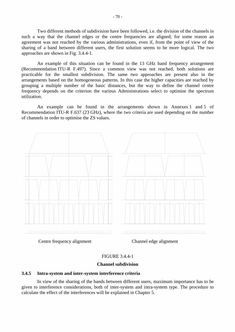
- 70 -

Two different methods of subdivision have been followed, i.e. the division of the channels in such a way that the channel edges or the centre frequencies are aligned; for some reason an agreement was not reached by the various administrations, even if, from the point of view of the sharing of a band between different users, the first solution seems to be more logical. The two approaches are shown in Fig. 3.4.4-1.

An example of this situation can be found in the 13 GHz band frequency arrangement (Recommendation ITU-R F.497). Since a common view was not reached, both solutions are practicable for the smallest subdivision. The same two approaches are present also in the arrangements based on the homogeneous patterns. In this case the higher capacities are reached by grouping a multiple number of the basic distances, but the way to define the channel centre frequency depends on the criterion the various Administrations select to optimise the spectrum utilization.

An example can be found in the arrangements shown in Annexes 1 and 5 of Recommendation ITU-R F.637 (23 GHz), where the two criteria are used depending on the number of channels in order to optimise the ZS values.

Centre frequency alignment Channel edge alignment

FIGURE 3.4.4-1

Channel subdivision

3.4.5 Intra-system and inter-system interference criteria

In view of the sharing of the bands between different users, maximum importance has to be given to interference considerations, both of inter-system and intra-system type. The procedure to calculate the effect of the interferences will be explained in Chapter 5.

- 71 -

This section will deal with the definition of the parameters involved and the impact on the selection of the optimised radio frequency arrangements.

As already anticipated, the choice between the different arrangements is directly related to the level of the interference among the channels and to the sensitivity of the receivers to the interferences. The relationships between the parameters have been shown in § 3.4.3.

It must be noted that, since the digital receivers are resistant against interference, a large overlap of spectra between adjacent channels can be accepted. This is the reason why, for example, it was possible to reuse analogue frequency arrangements (with smaller band occupancy) for digital transmission, where the occupied bands are larger.

It is important to verify, at this point, the applicability of the ITU definitions to the digital radio-relay systems.

As specified in Article 1, RR Nos. 146/147, two different definitions for the necessary bandwidth and the occupied bandwidth are given:

Necessary Bandwidth: For a given class of emission, the width of the frequency band which is just sufficient to ensure the transmission of information at the rate and with the quality required under specified conditions.

Occupied Bandwidth: The width of a frequency band such that, below the lower and above the upper frequency limits, the mean powers emitted are equal to a specified percentage β/2 of the total mean power of a given emission.

In the new Recommendation ITU-R F.1191, for DRRS the value of β/2 should be taken as 0.5%, hence the occupied bandwidth can be calculated by considering the bandwidth corresponding to 99% of the emitted spectrum.

This definition is valid also for other type of emissions covered by Recommendation ITU-R SM.328.

It was also agreed that the necessary bandwidth for DRRS is to be reasonably considered to have the same value as the occupied bandwidth.

Taking into account the effect of NFD and XPD as defined above, it is clear that it is not strictly necessary to make the occupied bandwidth always smaller than, or equal to, the bandwidth of the radio-frequency channel or, conversely, to fix the bandwidth of the radio-frequency channel equal to the necessary bandwidth.

According to the type of channel arrangement, the capacity and the modulation format, it was also agreed that a DRRS could have a necessary bandwidth up to 20% wider than the radio-frequency channel bandwidth.

The remaining 0.5% of the total transmitted mean power above and below the limits of the necessary bandwidth represents the unwanted emissions of the system.

A theoretical subdivision in the family of the Unwanted Emissions is defined in the RR (Article 1, Nos. 138 and 139) and results in:

a) Out-of-band Emission: Emission on a frequency or frequencies immediately outside the necessary bandwidth which results from the modulation process, but excluding spurious emissions.

- 72 -

b) Spurious emission: Emission on a frequency or frequencies which are outside the necessary bandwidth and the level of which may be reduced without affecting the corresponding transmission of information. Spurious emissions include harmonic emissions, parasitic emissions, intermodulation products and frequency conversion products, but exclude out-of band emissions.

As far as DRRS are concerned, since the effect of both will be to increase the level of interference into the system, no distinction has to be made between out-of band and spurious emissions; therefore they have to be considered together as unwanted emissions.

It should be noted that it is unlikely that out-of-band emissions from DRRS will cause significant interference into systems operating in adjacent bands, since the power spectrum of a DRRS decays rapidly outside the occupied bandwidth and the e.i.r.p. is low or medium.

The following Fig. 3.4.5-1 shows the unwanted emissions based on a typical heterodyne digital radio-relay transmitter; other emissions (e.g. conversion products and residual components of the carrier generation) are not shown. For directly modulated radio frequency transmitters, some unwanted emissions (e.g. conversion products and local oscillator leakage) are not applicable.

RF CHANNEL BANDWIDTH ADJACENT RF CHANNELS

Nth CLOCK LINES

IMAGE SIGNAL

LEAKAGE

THE WANTED SIGNAL (NOTE 1) AND OF

IF 2nd HARMONIC

(NOTE 2)(NOTE 2)

(NOTE 1)

THE LOCAL OSCILLATOR.(NOTE 2)

(NOTE 1)

ADJACENT BAND ALLOCATED TO FIXED SERVICE WITH

ESTABLISHED CHANNEL ARRANGEMENTS

NON ADJACENTADJACENT

PRODUCT)

ALLOCATED BANDALLOCATED BANDALLOCATED BAND

GUARDBAND3rd ORDER

(NOTES 1 AND 3) PRODUCT

Nth HARMONIC OF

INTERMODULATION

LOCAL OSCILLATOR

(CONVERSION PRODUCT)

(CONVERSION

NOTE 1 – Example of noise-like component of unwanted emissions. NOTE 2 – Example of discrete component of unwanted emissions. NOTE 3 – Non-linearity due to transmitter results in out-of-band emission which is immediately adjacent to the necessary bandwidth, due to odd-order intermodulation products.

FIGURE 3.4.5-1

Frequency bands and unwanted emissions of a digital radio-relay system (typical scenario)

- 73 -

3.5 Band sharing with other services

This section deals with interference between terrestrial fixed services (FS) and the fixed- satellite services (FSS). This has been the subject of investigation of Joint Radiocommunication Study Groups 4 and 9. This activity started in the early 1960s when it was decided that the new satellite communication systems would be sharing the 4 and 6 GHz bands that were heavily used for the critical long haul national backbone networks. The amount of interference that a satellite system could contribute to a terrestrial radio network has been limited to 11% of the overall interference budget of the terrestrial system. The remaining 89% is allocated to interference between terrestrial systems operating in the same frequency band. The ITU-R has recently issued the following series of Recommendations covering terrestrial interference: Recommendations ITU-R F.1094, ITU-R F.1095, ITU-R F.1096 and ITU-R F.1097. The reader is referred to § 5.3.5 for more information on terrestrial interference.

3.5.1 Assessment of interference from other services

3.5.1.1 General

Frequency sharing consideration has become a very important issue for system planners since many parts of the spectrum have recently been allocated to more than one service on a primary basis.

Radiocommunication Study Group 9 has actively carried out studies on the frequency sharing with the FSS through joint works with Radiocommunication Study Group 4, and successfully established Recommendations on the sharing criteria for both services.

After the Plenary Assembly in 1990 much efforts have been devoted to sharing issues with services other than the FSS. These resulted in Recommendations on protection criteria from the broadcasting-satellite service (BSS) in the bands near 20 GHz (Recommendation ITU-R F.760) or space stations operating in low-Earth-orbits (LEO) (Recommendation ITU-R F.1108).

There may be several stages in developing inter-service sharing studies, the goal of which is to adopt Recommendations on basic system parameters (such as e.i.r.p.) or, from a practical point of view, Recommendations on coordination distance between terrestrial radio stations and earth stations. As a preparation for the above, it may be necessary to establish Recommendations on protection criteria, i.e. allowable performance and availability degradation due to interference from each other service.

An example of the development of frequency sharing studies is presented below: Stage 1: General considerations. Stage 2: Assessment of inter-service interferences using certain models. Stage 3: Adoption of Recommendations on allowable performance and availability degradation objectives. Stage 4: Adoption of Recommendations on basic system parameters.

Studies on sharing with the FSS have reached stage 3 or 4 in many parameters, while many of those on other space or terrestrial services are under 1 or 2 stages.

3.5.1.2 Degradation in performance and availability

In the assessment of interference to the FS, effects on the circuit performance should be analysed by considering not only the absolute power of the interfering wave but also its frequency spectrum and occurrence probability. Interfering waves are subdivided into two categories in terms of amplitude probability distributions: Category 1: Gaussian interference Category 2: Non-Gaussian interference

- 74 -

There are many types of non-Gaussian interference, among which carrier-wave (sinusoidal wave) interference may be a typical one. Since Gaussian noise has a large peak factor in its amplitude distribution, assumption of unknown interference to be Gaussian interference leads to safety assessment for the interfered-with side and, at the same time, tight requirements for the interfering side.

Interfering waves can also be classified in terms of occurrence modes as follows:

i) stationary interference, ii) non-stationary interference,

ii-1) periodic interference, ii-2) non-periodic interference.

Stationary interference noise, as far as its amplitude follows the Gaussian distribution, can be handled in the same way as thermal noise having the same power. As illustrated in Fig. 3.5.1-1, stationary interference noise (Ns) contributes to the reduction of the carrier-to-noise ratio, resulting in smaller fading margin Fd ' and larger occurrence probability of severely errored seconds (SES). Thus, the effects of stationary interference noise (for example that from space stations on the geostationary-satellite orbit (GSO)) can be evaluated by the power ratio to the total noise power. Actually the interference criteria given in Recommendation ITU-R SF.615 specify the increase of the error occurrence probability in the performance and availability objectives for digital radio-relay systems.

time

FIGURE 3.5.1-1

Effects of stationary interference noise

Non-stationary interference can be further subdivided into periodic interference (such as that from low-Earth-orbit satellites) and non-periodic interference (such as unwanted emissions from mobile radar systems). These interferences are normally below a tangible level, however they may produce harmful effects when interference sources traverse the main beam of the antenna of the

- 75 -

interfered-with stations. The effects pose a problem when the interference noise causes bit errors even during non-faded periods. In many cases, a noise burst of the non-stationary interference (Ni) alone dominates the total noise with little contribution from other stationary noises (see Fig. 3.5.1-2). Since simultaneous occurrence probability of an interference-noise burst and deep fading of the desired signal is usually negligible, non-stationary interference therefore could be assessed by only the occurrence probability of harmful noise bursts affecting the increase of SES or ES (see ∆T0, ∆Ti in Fig. 3.5.1-2). Therefore it is necessary to clarify the cumulative distribution of Ni or the corresponding power flux density (PFD) with respect to time percentage.

time

FIGURE 3.5.1-2 Effects of non-stationary interference noise

Also for availability degradation the same discussion on Figs. 3.5.1-1 and 3.5.1-2 can be applied to the rain fade margin reduction or noise burst lasting for more than 10 s.

In case of non-periodic interference it is usually difficult to clarify through statistical approach the relationship between ∆T0 and Ni. The protected criteria have to be derived from analyses using a certain calculation model. It should be noted that non-periodic interference arises not only from mobile sources but also can be observed in emissions from space stations on GSO when the arrival angle is low and the propagation condition becomes anomalous.

The subjects of establishing interference criteria with services in non-shared environments are generally called “compatibility” which means the guarantee for acceptable operation of both services. Radiocommunication Study Group 9 is also studying such a kind of interference issue from radar systems in consultation with Radiocommunication Study Group 8.

3.5.1.3 Assessment of aggregate effects of interference from various sources

In link design of DRRS interference noise should be assessed in its overall contribution to system outage. In this connection ITU-R has adopted a new Recommendation ITU-R F.1094 specifying the limit of relative contribution for various kinds of emissions (see Fig. 3.5.1-3). According to that Recommendation interference noise is categorized into the following three groups:

- 76 -

– Category X: Emissions from radio-relay systems operating in the same band.

– Category Y: Emissions from other radio services which share frequency allocations on a primary basis.

– Category Z: Emissions from radio services which share frequency allocations on a non- primary basis; or

Unwanted emissions (i.e. out-of-band and spurious emissions such as energy spread from radio systems, etc.) in non-shared bands; or

Unwanted radiation (e.g. ISM applications). Assuming that the contribution on performance (or availability) degradation from each category be X%, Y% and Z%, respectively, it is recommended that the aggregate effect of X + Y + Z (=100%) should not cause the violation of error performance (or availability) objectives given in the relevant Recommendations (§ 3.2). As for the subdivision of X, Y and Z the following values are recommended:

X = 89 (%) (3.5.1-1a) Y = 10 (%) (3.5.1-1b) Z = 1 (%) (3.5.1-1c) The value of Y (=10%) is based on the conventional criteria in Recommendation ITU-R SF.615 with the fixed-satellite service. However, in the frequency bands shared by services other than FS and FSS on the primary basis, the value 10% should be further subdivided also into these services.

FIGURE 3.5.1-3

RF interference sources

- 77 -

The ratio given by equations (3.5.1-1a) to (1c) is not necessarily satisfied in each radio hop, but should be assessed over the reference link length specified in each Recommendation (i.e. in case of systems used in the high grade portion; 2 500 km). Therefore, in a certain radio hop where the DRRS is exposed to severe interference from other services, the value of Y can become much larger. Such an example is given below.

Assuming that the total outage period due to long-term interference is in a single hop exposed to interference from an earth station, then the permissible outage on that hop due to thermal noise and interference is 6.55 times that on the remaining hops of the hypothetical reference digital path (HRDP). This can be shown by assuming that the total permissible interference in a 50 hop HRDP should account for 10% of the total permissible outage.

(3.5.1-2)

where:

pu: total permissible outage in the HRDP in percentage of the time.

This yields Yi = 5 = 500(%)

However, in real cases, a minimum value of Yi is usually selected to be less than the above case considering possible increase of satellite interference in the future.

3.5.2 Basic parameters for sharing considerations

3.5.2.1 Receiver side

Power flux density (pfd) produced by the interfering wave is the most important parameter for the interfered-with side in sharing considerations. The maximum allowable pfd can be given by the following equation:

(pfd) + 10 log Ar + 10 log B – Lr = Ir (3.5.2-1)

Ir < C – (C/I)0 (3.5.2-2)

or:

Ir < NTH – P = – 10 log (kTB) + F – P (3.5.2-3)

where:

(pfd) : power flux-density (dB(W/m2/MHz)) Ar : effective receive antenna aperture (m2) B : receiver bandwidth (MHz) Lr : feeder/waveguide loss (dB) Ir : interference noise level (dBW) C : signal power (dBW) (C/I)0 : carrier-to-noise ratio for references BERs (dB) NTH : thermal noise level (dBW) F : receiver noise figure (dB) P : relative reduction factor (dB)

- 78 -

In the method using equation (3.5.2-2) the reference BER is usually selected to be 10-3 (short-term interference) or 10-6 (long-term interference). Then the values (C/I)0 and Ir can be calculated according to the modulation scheme.

On the other hand the method using equation (3.5.2-3) more simply determines the value Ir for every modulation scheme solely depending on the receiver characteristics. The parameter P is decided by how much reduction in the fade margin can be allowed in the presence of the interference. Typically the following values in Table 3.5.2-1 are used.

TABLE 3.5.2.-1

P (dB)

Fade margin reduction (dB)

10 0.5 6 1

It should be noted that the maximum allowable pfd derived from the equation (3.5.2-1) applies to in-beam interference. For off-beam interference more pfd can be allowed according to the directivity of the receive antenna.

Therefore the maximum allowable pfd increase is proportional to the arrival angle θ except when θ is smaller than 5° or larger than 25° (see Fig. 3.5.2-1).

FIGURE 3.5.2-1 Power flux-density limits

Specifications for the PFD limits are generally given in the following manner:

P1 dB(W/m2) for θ ≤ 5º

P1 + 0.05(p2 - p1) (θ - 5) dB(W/m2) for 5º < θ ≤ 25º

P2 dB(W/m2) for 25º < θ ≤ 90º

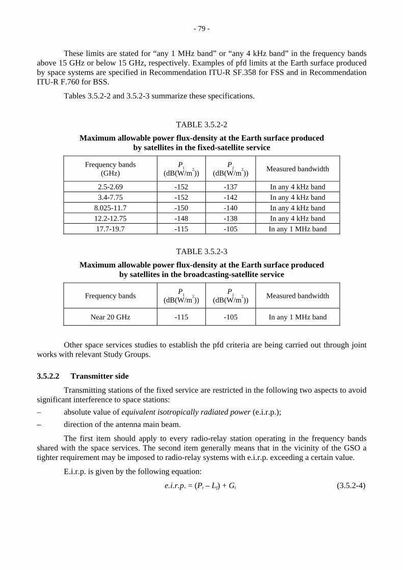
- 79 -

These limits are stated for “any 1 MHz band” or “any 4 kHz band” in the frequency bands above 15 GHz or below 15 GHz, respectively. Examples of pfd limits at the Earth surface produced by space systems are specified in Recommendation ITU-R SF.358 for FSS and in Recommendation ITU-R F.760 for BSS.

Tables 3.5.2-2 and 3.5.2-3 summarize these specifications.

TABLE 3.5.2-2

Maximum allowable power flux-density at the Earth surface produced by satellites in the fixed-satellite service

Frequency bands (GHz)

P1 (dB(W/m

2))

P2 (dB(W/m

2)) Measured bandwidth

2.5-2.69 -152 -137 In any 4 kHz band 3.4-7.75 -152 -142 In any 4 kHz band

8.025-11.7 -150 -140 In any 4 kHz band 12.2-12.75 -148 -138 In any 4 kHz band 17.7-19.7 -115 -105 In any 1 MHz band

TABLE 3.5.2-3

Maximum allowable power flux-density at the Earth surface produced by satellites in the broadcasting-satellite service

Frequency bands P1 (dB(W/m

2))

P2 (dB(W/m

2)) Measured bandwidth

Near 20 GHz -115 -105 In any 1 MHz band

Other space services studies to establish the pfd criteria are being carried out through joint works with relevant Study Groups.

3.5.2.2 Transmitter side

Transmitting stations of the fixed service are restricted in the following two aspects to avoid significant interference to space stations:

– absolute value of equivalent isotropically radiated power (e.i.r.p.);

– direction of the antenna main beam.

The first item should apply to every radio-relay station operating in the frequency bands shared with the space services. The second item generally means that in the vicinity of the GSO a tighter requirement may be imposed to radio-relay systems with e.i.r.p. exceeding a certain value.

E.i.r.p. is given by the following equation:

e.i.r.p. = (Pt – Lf) + Gt (3.5.2-4)

- 80 -

where:

Pt : transmitter power

Lf : feeder loss

Gt : transmit antenna gain.

In equation (3.5.2-4) (Pt – Lf) means the power delivered to the antenna input, which is also a parameter to be specified.

Specifications of e.i.r.p. limits can be represented by Fig. 3.5.2-2. In this figure the angle θ means the azimuth of the transmit antenna. On the other hand the radius of the circles (e1,e2) denotes the limit of e.i.r.p.

Thus, space stations on the GSO are protected by the tighter e.i.r.p. limit with a protection angle, α. In other words the maximum radiation direction of any antenna at a radio-relay station with e.i.r.p higher than e2 should be at least α degrees away from GSO. According to the specifications in Recommendation ITU-R SF.406 the upper limit e1 is +55 dBW in all the frequency bands shared with the fixed-satellite service, while the value e2 and protection angle α depend on the frequency band (see Table 3.5.2-4). For the inter-satellite service it is being studied to specify only the limit e2 in the frequency band above 20 GHz.

FIGURE 3.5.2-2

Concept of the e.i.r.p. limit

- 81 -

TABLE 3.5.2-4

E.i.r.p. limit for radio-relay stations operating in the frequency bands shared with the fixed-satellite service

Frequency bands (GHz)

(Pt - Lf) (dBW)

e1 (dBW)

e2(1) (dBW)

α(1) (degrees)

1 to 10 +13 35 2

10 to 15 +10 +55 45 1.5

Above 15 +10 – –

(1) These values should be met as far as practicable. For the cases that it is impracticable the restrictions are given in Recommendation ITU-R SF.406.

In addition to the above restrictions various protection criteria have been proposed for many space services. However, most of them are now under study.

TABLE 3.5.3-1

Radiocommunication Study Group 9 texts on inter-service frequency sharing

Services Subjects or frequency bands Recommendations

All services General methodology ITU-R F.758 ITU-R F.1094

General methodology ITU-R SF.355

Interference criteria (for analogue systems)

ITU-R SF.357

Fixed-satellite Interference criteria (for digital systems)

ITU-R SF.615

PFD(1) limits e.i.r.p. limits

ITU-R SF.358 ITU-R SF.406

Broadcasting-satellite (17.7-17.8, 21.4-22) GHz ITU-R F.760

Space research 18.6-18.8 GHz ITU-R F.761

Space services using GSO Visibility statistics for all frequency bands

ITU-R F.1107

Space services using LEO FDP(2) limits ITU-R F.1108

Fixed-satellite and other services(3)

Coordination area ITU-R IS.847

(Radar system) Interference mitigation options ITU-R F.1097

Radiodetermination Protection criteria to ensure compatibility

ITU-R F.1190

(1) Power flux-density. (2) Fractional degradation in performance. (3) Meteorological-satellite, Earth exploration-satellite, space research and space operation.

- 82 -

3.5.3 Status of studies on frequency sharing within Radiocommunication Study Group 9

Studies on sharing issues within Radiocommunication Study Group 9 are conducted in two Working Parties. Frequency sharing with Radiocommunication the fixed-satellite service (FSS) has been studied in Radiocommunication Working Party 4-9S, the joint party with Radiocommunication Study Group 4. In this field many Recommendations have already been established and they are incorporated in a separate volume as the ITU-R SF Series. On the other hand sharing subjects with services other than FSS are the terms of reference of Working Party 9D. Working Party-9D are now actively engaged in various sharing criteria through joint works with Radiocommunication Study Groups 7, 8, 10 and 11.

The texts listed in Table 3.5.3-1 summarize typical Recommendations which would provide an informative basis for system planners.

- 83 -

REFERENCES TO CHAPTER 3

ITU-R Recommendations:

Rec. ITU-R F.497 Radio-frequency channel arrangements for radio-relay systems operating in the 13 GHz frequency band.

Rec. ITU-R F.556 Hypothetical reference digital path for radio-relay systems which may form part of an integrated services digital network with a capacity above the second hierarchical level.

Rec. ITU-R F.557 Availability objective for radio-relay systems over a hypothetical reference circuit and a hypothetical reference digital path.

Rec. ITU-R F.594 Allowable bit error ratios at the output of the hypothetical reference digital path for radio-relay systems which may form part of an integrated services digital network.

Rec. ITU-R F.634 Error performance objectives for real digital radio-relay links forming part of a high-grade circuit within an integrated service digital network.

Rec. ITU-R F.637 Radio-frequency channel arrangements for radio-relay systems operating in the 23 GHz band.

Rec. ITU-R F.695 Availability objectives for real digital radio-relay links forming part of a high-grade circuit within an integrated services digital network.

Rec. ITU-R F.696 Error performance and availability objectives for hypothetical reference digital sections utilizing digital radio-relay systems forming part or all of the medium-grade portion of an ISDN connection.

Rec. ITU-R F.697 Error performance and availability objectives for the local-grade portion at each end of an ISDN connection utilizing digital radio-relay systems.

Rec. ITU-R F.746 Radio-frequency channel arrangements for radio-relay systems.

Rec. ITU-R F.756 TDMA point-to-multipoint systems used as radio concentrators.

Rec. ITU-R F.758 Considerations in the development of criteria for sharing between the terrestrial fixed service and other services.

Rec. ITU-R F.760 Protection of terrestrial line-of-sight radio-relay systems against interference from the broadcasting-satellite service in the bands near 20 GHz.

Rec. ITU-R F.761 Frequency sharing between the fixed service and passive sensors in the band 18.6-18.8 GHz.

- 84 -


Rec. ITU-R F.1094 Maximum allowable error performance and availability degradations to digital radio-relay systems arising from interference from emissions and radiations from other sources.

Rec. ITU-R F.1095 A procedure for determining coordination area between radio-relay stations of the fixed service.

Rec. ITU-R F.1096 Methods of calculating line-of-sight interference into radio-relay systems to account for terrain scattering.

Rec. ITU-R F.1097 Interference mitigation options to enhance compatibility between radar systems and digital radio-relay systems.

Rec. ITU-R F.1107 Probabilistic analysis for calculating interference into the fixed service from satellites occupying the geostationary orbit.

Rec. ITU-R F.1108 Determination of the criteria to protect fixed service receivers from the emissions of space stations operating in non-geostationary orbits in shared frequency bands.

Rec. ITU-R F.1190 Protection criteria for digital radio-relay systems to ensure compatibility with radar systems in the radiodetermination service.

Rec. ITU-R F.1191 Bandwidths and unwanted emissions of digital radio-relay systems.

Rec. ITU-R SF.355 Frequency sharing between systems in the fixed-satellite service and radio-relay systems in the same frequency bands.

Rec. ITU-R SF.357 Maximum allowable values of interference in a telephone channel of an analogue angle-modulated radio-relay system sharing the same frequency bands as systems in the fixed-satellite service.

Rec. ITU-R SF.358 Maximum permissible values of power flux-density at the surface of the Earth produced by satellites in the fixed-satellite service using the same frequency bands above 1 GHz as line-of-sight radio-relay systems.

Rec. ITU-R SF.406 Maximum equivalent isotropically radiated power of radio-relay system transmitters operating in the frequency bands shared with the fixed-satellite service.

Rec. ITU-R SF.615 Maximum allowable values of interference from the fixed-satellite service into terrestrial radio-relay systems which may form part of an ISDN and share the same frequency band below 15 GHz.

Rec. ITU-R IS.847 Determination of the coordination area of an earth station operating with a geostationary space station and using the same frequency band as a system in a terrestrial service.

Rec. ITU-R SM.328 Spectra and bandwidth of emissions.

- 85 -

ITU-R Documents (1996)

ITU-R Draft Recommendation [Doc. 9/12] Radio-frequency channel arrangements for digital radio systems operating in the range 1 350 MHz to 1 530 MHz.

ITU-R Draft Recommendation [Doc. 9/13] Radio-frequency channel arrangements for digital radio systems operating in the range 2 290-2 670 MHz.

ITU-R Draft Recommendation [Doc. 9/14] Radio Local Area Networks (RLAN).

ITU-T Recommendations

ITU-T Rec. G.702 Digital hierarchy bit rates.


ITU- T Rec. G.704 Synchronous frame structures used at primary and secondary hierarchical levels.

ITU-T Rec. G.707 Synchronous digital hierarchy bit rates.

ITU-T Rec. G.708 Network node interface for the synchronous digital hierarchy.

ITU-T Rec. G.709 Synchronous multiplexing structure.

ITU-T Rec. G.783 Characteristics of synchronous digital hierarchy (SDH) equipment functional blocks.

ITU-T Rec. G.784 Synchronous digital hierarchy (SDH) management.

ITU-T Rec. G.821 Error performance of an international digital connection forming part of an integrated services digital network.

ITU-T Rec. G.822 Controlled slip rate objectives on an international digital connection.


ITU-T Rec. M.20 Maintenance philosophy for telecommunication networks.

ITU-T Rec. M.32 Principles for using alarm information for maintenance of international transmission systems and equipment.

ITU-T Rec. M.34 Performance monitoring on international transmission systems and equipment.

ITU-T Rec. M.2100 Performance limits for bringing-into-service and maintenance of international PDH paths, sections and transmission systems.

ITU-T Rec. M.2101 Performance limits for bringing-into-service and maintenance of international SDH paths and multiplex sections.

ITU-T Rec. M.2110 Bringing-into-service international digital path, sections and transmission systems.

ITU-T Rec. M.2120 Digital path, section and transmission system fault detection and localization procedures.

- 86 -

CHAPTER 4

DESIGN PARAMETERS

4.1 Propagation related issues

4.1.1 Concept of free space loss

The radiated electromagnetic energy wave front propagates in the direction in which it was focused by the reflector in an ever expanding wave front. This expansion is essentially done according to the well known Inverse Square law of radiation. The free space loss (FSL) is a result of this expanding wave front and its value is given in equation (4.1.1-1) below. In this equation for FSL, the transmitter and the receiver have been assumed as isotropic radiators, meaning that the wave front is expanding uniformly in every direction and that no directive elements have been used. To take into account antenna directivity, the gain of TX and RX antennas have to be added separately.

FSL f d= + +92 44 20 20. log( ) log( ) (4.1.1-1)

where: FSL : free space loss (dB) f : frequency of radio (GHz) d : distance between transmitter and receiver (km).

Figure 4.1.1-1 provides a plot of FSL for various distances and for various frequencies. Also refer to the ITU-R P Series Recommendations (see Recommendation ITU-R P.525).

4 8 12 16 20 24 28 32 36 40 44 48

150

140

130

120

110

2 GHz

4 GHz

6 GHz

7 GHz

10 GHz

15 GHz

Distance (km)

FIGURE 4.1.1-1

Free space loss versus distance (for various frequencies)

- 87 -

4.1.2 Visibility

4.1.2.1 Refractive aspects

Terrestrial line-of-sight propagation is influenced by vertical variations in the refractive index of the atmosphere. Because of refraction, microwaves travel along slightly curved paths.

Under normal propagation conditions the radio path is bent downwards so that the radio horizon is effectively extended. Particular conditions may occur such as positive values of the refractivity gradient so that the radio path is bent upwards. When the radio path is low enough so that part of it grazes the ground, diffraction effects, giving rise to received signal level reductions may occur (obstruction fading). In extreme cases, the ground obstacle may actually intercept the whole radio beam causing a complete loss of visibility between transmitting and receiving antennas with a consequent received signal too small to be used.

An important objective in planning terrestrial microwave links is to design the path in such a way that losses of visibility are extremely rare events. To do that, an accurate knowledge both of terrain profile between the terminals and of refractivity gradient variations is needed. Sufficient path clearance should be guaranteed for the most important subrefractive conditions expected on the path, through a proper choice of antenna heights, which also should not be greater than actually needed.

The parameter generally used to describe the spatial and temporal variations of the radio refractive index n is the radio refractivity N defined as:

N n= −( )1 106 in N-units (4.1.2-1)

At radio frequencies up to 100 GHz with an error less than 0.5 %, the refractivity N can be approximately expressed by the Bean and Dutton relationship [Bean and Dutton, 1966]

NPT

eT

= + ×77 6 373 1052. . (4.1.2-2)

where:

P : atmospheric pressure (hPa)

T : absolute temperature (K)

e : water vapour pressure (hPa).

N varies primarily with height. The vertical variation in the lowest layer of the atmosphere is of most importance to the calculation of refraction effects and is described by the refractivity gradient G as follow:

GNh

= dd

(N-units/km) (4.1.2-3)

where h is the height (km).

In average conditions the refractivity dependence with height is provided by the standard atmosphere model according to the following exponential law (see Recommendation ITU-R P.369):

N N h hs s= −0 0exp( / ) (4.1.2-4)

- 88 -

where Ns is the N value at height hs (km) above sea level and the constants N0 and h0 are given by:

N0 315= N-units, and

h0 7 35= . km

where N0 is the average value of radio refractivity at the surface of the Earth. More precise values of N0 for all the world can be found in Figs. 1 and 2 of Recommendation ITU-R P.453. According to equation (4.1.2-4) the refractivity gradient in the average conditions results in a refractivity gradient value of -43 N-units/km for the lower atmosphere layers.

Under the assumption of a constant refractivity gradient G it can be shown that a radio ray has a curvature radius expressed approximately by:

r

G= − 106

(r (km) and G (N-units/km)) (4.1.2-5)

where the minus sign indicates that the ray bending is towards the Earth’s surface (see Recommendation ITU-R P.834).

A well-known transformation allows propagation to be considered as rectilinear above a hypothetical Earth effective radius ae according to:

1 1 1

a a re= − (4.1.2-6)

where a is the actual Earth radius (a = 6 370 km).

As from equation (4.1.2-5), r depends on the refractivity gradient G, as does the effective equivalent Earth radius ae.

If k (denoted as k-factor) is the multiplication factor between a and ae according to ae= k a, then from equations (4.1.2-5) and (4.1.2-6) k is related to G as follows:

k = 157

157 + G (4.1.2-7)

where the value 157 represents approximately the ratio between 106 and the actual Earth radius a.

In a standard atmosphere k assumes a value of about 4/3.

Figure 4.1.2-1 shows the reference geometry for the equivalent Earth model. For practical reasons a simpler geometry is generally adopted as shown in Fig. 4.1.2-2. The major advantage using the equivalent Earth model is that, with reference to Fig. 4.1.2-2, the ray path trajectory H(x) is immediately obtained and drawn once the two heights h1, h2 and the hop length d are known. It can be shown that the equivalent Earth bulge curve can be B(x) approximately represented by the following equation:

B xk a

d x( ) ( )= × −12

(4.1.2-8)

The ray elevation at a point x along the ground path is E(x) = H(x) - B(x).

- 89 -

d

ka

h1 h2

ray path

FIGURE 4.1.2-1

Equivalent Earth model reference geometry

FIGURE 4.1.2-2

Practical equivalent Earth model reference geometry

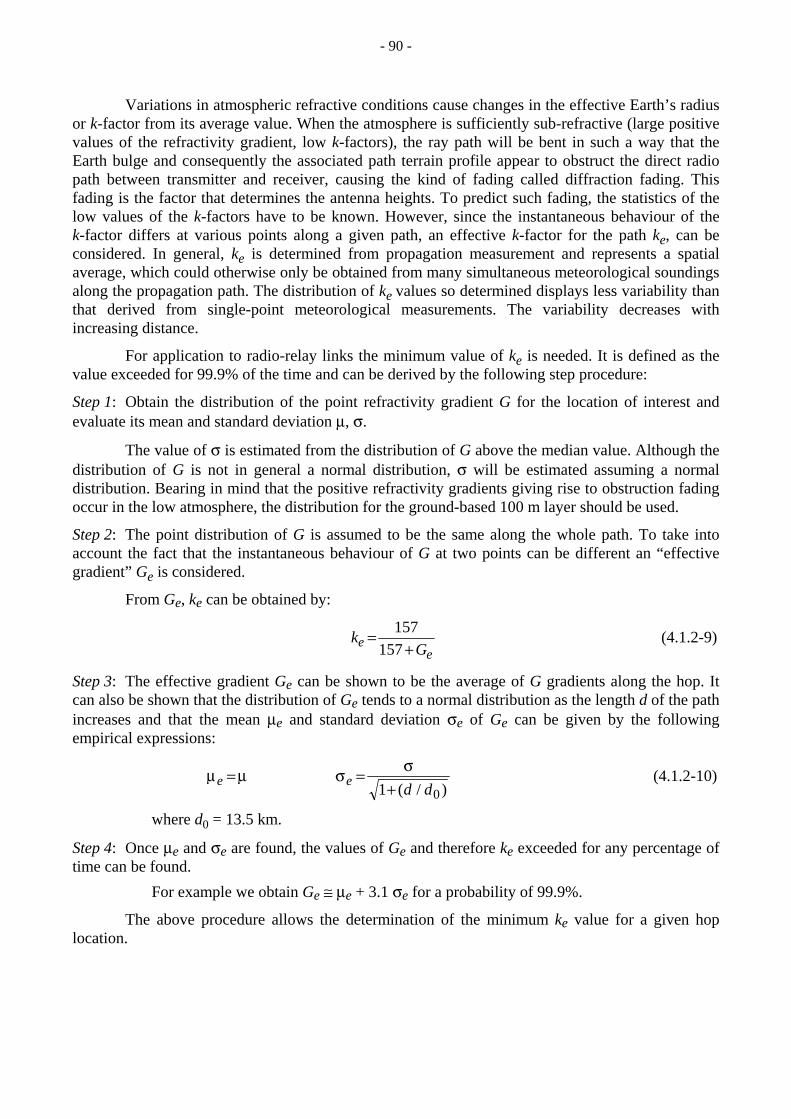
- 90 -

Variations in atmospheric refractive conditions cause changes in the effective Earth’s radius or k-factor from its average value. When the atmosphere is sufficiently sub-refractive (large positive values of the refractivity gradient, low k-factors), the ray path will be bent in such a way that the Earth bulge and consequently the associated path terrain profile appear to obstruct the direct radio path between transmitter and receiver, causing the kind of fading called diffraction fading. This fading is the factor that determines the antenna heights. To predict such fading, the statistics of the low values of the k-factors have to be known. However, since the instantaneous behaviour of the k-factor differs at various points along a given path, an effective k-factor for the path ke, can be considered. In general, ke is determined from propagation measurement and represents a spatial average, which could otherwise only be obtained from many simultaneous meteorological soundings along the propagation path. The distribution of ke values so determined displays less variability than that derived from single-point meteorological measurements. The variability decreases with increasing distance.

For application to radio-relay links the minimum value of ke is needed. It is defined as the value exceeded for 99.9% of the time and can be derived by the following step procedure:

Step 1: Obtain the distribution of the point refractivity gradient G for the location of interest and evaluate its mean and standard deviation µ, σ.

The value of σ is estimated from the distribution of G above the median value. Although the distribution of G is not in general a normal distribution, σ will be estimated assuming a normal distribution. Bearing in mind that the positive refractivity gradients giving rise to obstruction fading occur in the low atmosphere, the distribution for the ground-based 100 m layer should be used.

Step 2: The point distribution of G is assumed to be the same along the whole path. To take into account the fact that the instantaneous behaviour of G at two points can be different an “effective gradient” Ge is considered.

From Ge, ke can be obtained by:

kGe

e=

+157

157 (4.1.2-9)

Step 3: The effective gradient Ge can be shown to be the average of G gradients along the hop. It can also be shown that the distribution of Ge tends to a normal distribution as the length d of the path increases and that the mean µe and standard deviation σe of Ge can be given by the following empirical expressions:

µ µe = σ σe d d

=+1 0( / )

(4.1.2-10)

where d0 = 13.5 km.

Step 4: Once µe and σe are found, the values of Ge and therefore ke exceeded for any percentage of time can be found.

For example we obtain Ge ≅ µe + 3.1 σe for a probability of 99.9%.

The above procedure allows the determination of the minimum ke value for a given hop location.

- 91 -

For continental temperate climate, a ke value exceeded for approximately 99.9% of the worst month can be obtained directly from Fig. 4.1.2-3 (see Recommendation ITU-R P.530).

FIGURE 4.1.2-3

Value of ke, exceeded for approximately 99.9% of the worst month (continental temperate climate)

4.1.2.2 Path profiles, clearance and obstructions

Radio waves would travel through the atmosphere in straight lines if the atmospheric density, or radio refractivity N, were constant. This is normally not the case and refractivity gradually diminishes with height h above the ground. In atmospheres that have a constant refractivity gradient dN/dh but otherwise are uniform, a radio ray travels in a circle. This has to be taken into account when the radio ray is drawn in the vertical plane that contains the terrain profile, the so-called path profiles (see Fig. 4.1.2-4).

d

FIGURE 4.1.2-4 Elevated Earth path profile

- 92 -

There are several possibilities to draw such profiles. One is to show the true radio ray above the Earth’s surface represented by a circle and the actual Earth radius a = 6 370 km. A second method is to straighten the circular radio ray into a straight line and correct for this by changing the Earth radius to k a, where k is the Earth radius factor, as seen in Fig. 4.1.2-1

A third method, to be used in the following, is to make the Earth’s surface flat and use a circle of radius k a for the radio ray. This flat Earth method has the advantage that the terrain profile doesn’t have to be redrawn each time the k factor is changed. It is much simpler to redraw the ray circle than to redraw a complex terrain profile over a changing Earth radius.

An example of using the flat Earth method is shown in Fig. 4.1.2-5 for a 2 GHz hop 40 km long. The profile of the terrain may be obtained from maps by reading at regular intervals along the line-of-sight the highest contour at a distance of 50-100 m on each side. While preliminary path profiles used for path feasibility assessment may only need a few readings in addition to the highest points of the hop, accurate design often requires more to ensure that clearance criteria are met.

It should also be noted that the ITU-R performance prediction methods prescribe reading elevations at 1 km intervals for accurate calculation of the surface roughness factor.

In Fig. 4.1.2-5 four radio trajectories plotted for k values of 0.5, 4/3, ∞ and -2/3. The value k = 4/3 belongs to the standard atmosphere, k = 0.6 refers to a sub refractive atmosphere that can lead to obstruction fading, and k = -2/3 is for a super refractive atmosphere which can be the source of reflecting layers and multipath fading.

20

0

– 20

– 40

– 60

– 80

– 100

– 1204035302520151050

R

T

x (m

)

z (km)

k = – 2/3

∞

4/3

0.5

FIGURE 4.1.2-5

Microwave rays in a constant k atmosphere and path profile - flat Earth model

- 93 -

The circular radio rays in Fig. 4.1.2-5 were generated with the following formulas [Giger, 1991]:

x = [z sin ϕt + z2/2k.a]/ cos ϕt (4.1.2-11)

where:

ϕt = arc tan(xr/zr) - arc sin[ (xr2 + zr2 )0.5/2k.a] (4.1.2-12)

The origin of the (z - x) coordinate system is at the transmitting antenna T and the receiving antenna R is at z = zr (horizontal distance) and x = xr (vertical distance with respect to the transmitting antenna). The radio trajectory leaves the transmitter T at an angle ϕt to the local horizontal. Sometimes we also like to know the angle ϕz that the ray forms with the horizontal anywhere along the path at distance z:

ϕz = arc tan [sin ϕt + z/k.a] / cos ϕt (4.1.2-13)

This formula can be used to calculate the arrival angle at the receiver R or at any point on the ground, if R is moved along the terrain profile for purposes of studying ground reflections, for instance.

4.1.2.3 Diffraction aspects

The property of diffraction manifests itself as a bending of the electromagnetic waves around an obstacle such as a sharp knife edge or a spherical surface. The phenomenon is explained by classical Huyghens’ theory, which assumes that every point on the wave front has the property of generating secondary waves. Thus it is not necessary for the signal to be received only through line-of-sight path, but reception is possible, especially in the shadow regions, through secondary/tertiary or even higher order waves. This property of bending is related to the wavelength and to the dimensions of the obstacle, being more pronounced for higher wavelengths and for sharper obstacles. Also refer to Recommendation ITU-R P.526.

The importance of diffraction for microwave engineers is that obstacles which are in close proximity to the microwave beam can affect propagation conditions and can cause additional losses during propagation. A particular important concept is the Fresnel Zones (FZ) or Fresnel ellipsoides. The Fresnel zones are defined as ellipsoids of revolution, with the major axis lying on the line-of-sight, and the radius (width) at any point determined such that the difference in path length between the direct ray and the ray reflected at the surface of the ellipsoid is an integral multiple n (or nf) of half a wavelength. The focal points of ellipsoids are transmission and reception points. The concept is shown in Fig. 4.1.2-6.

The radius of the “nth” ellipsoid at a point between the transmitter and the receiver is given by the following formula, in practical units:

Fnd d

d d fn =+

⎡

⎣⎢

⎤

⎦⎥5501 2

1 2

1 2( )

/ (4.1.2.-14)

where f is the frequency (MHz) and d1 and d2 are the distances (km) between transmitter and receiver at the point for which the ellipsoid radius is calculated. Fn is in metres.

- 94 -

Going back to Fig. 4.1.2-5 we see that the radio rays pass freely from transmitter to receiver, even for a k factor as low as 0.5. We know from diffraction theory that a ray that just clears the top of a knife edge (which is an approximation for our hill at 12.5 km) would be attenuated by 6 dB compared to free space transmission. This loss can be avoided if there is some clearance between the ray and the obstruction, normally expressed in terms of the first Fresnel zone or ellipse. The major axis of the first Fresnel ellipse lies on the direct ray from T to R, and the ellipse itself is the locus of all reflection points which produce signals at the receiver that are delayed by ∆ = 0.5 λ with respect to the direct ray. The equation of the Fresnel ellipse, superimposed on the direct ray is as follows:

x = [z sin ϕt + z2/2ka]/ cos ϕt + nf λ z [1 - (z/zr) ] 0.5 (4.1.2-15)

where λ is the wavelength and nf the Fresnel number, which is equal to ∆ = 0.5 λ.

Figure 4.1.2-7 shows diffraction losses for the knife edge and other obstacles. We see that a clearance of as little as 30% of the first Fresnel zone produces the free space signal level. It has been the custom, however, to design radio paths that have full first Fresnel zone clearance for k = 4/3. An additional requirement is to avoid obstruction fading by having some clearance left for the lowest expected k factor. Often a value of kmin = 0.5 to 0.7 is used in path design. The clearance at the lower limit of k can be less than one Fresnel zone because during this exceptional atmospheric condition we still have a large fade margin (typically a reserve of 40 dB) available in our radio equipment. It should also be noted, that too large a clearance beyond the first Fresnel zone will produce unwanted variations of signal levels as the k-factor varies.

d2d1

F1

F2

d

d + λ / 2

d + 2 λ / 2

Plane perpendicularto direct ray

RxTx Direct ray

FIGURE 4.1.2-6

Three-dimensional representation of Fresnel zone

The effect of signal strength on path clearances in terms of the first Fresnel zone radius is shown in Fig. 4.1.2-7.

- 95 -

4

0

– 4

– 8

– 12

– 16

– 20

– 24

1 2 3 4 50nf

1

3

2

Rec

eive

d le

vel r

elat

ive

tofr

ee s

pace

val

ue (d

B)

FIGURE 4.1.2-7

Diffraction loss

n f ≅Actual clearance

First Fresnel zone clearance

1: Knife edge 2: Smooth spherical Earth 3: Intermediate terrain

We illustrate the clearance requirements for k = 4/3 in Fig. 4.1.2-8 where equation (4.1.2-15) has been used to draw a number of Fresnel ellipses. We show ellipses beginning with the first Fresnel zone, where nf = 1, and continuing in steps of 0.25 up to the second Fresnel zone, where nf = 2. We see that the peak of the hill, which is the closest obstacle to the direct ray, meets the requirement of first Fresnel zone clearance. If this were not the case either the transmitting or receiving antenna height would have to be increased.

As a practical rule, propagation is assumed to occur in line-of-sight, i.e. with negligible diffraction phenomena, if there is no obstacle within the first Fresnel ellipsoid.

A further point to notice is the inclination of the line-of-sight with respect to the horizontal. In general, it has been practice among many designers to avoid purely horizontal lines-of-sight and possibly to aim at so-called slant paths. The ITU-R performance prediction model makes use of theoretical and practical research on the effects of path-inclination, which in this model contributes explicitly to the outcome of the calculations.

- 96 -

FIGURE 4.1.2-8

Path profile with Fresnel ellipses for k = 4/3 and 2 GHz

Whichever method of path design is chosen, it often requires several iterations to arrive at the optimum result regarding minimum tower heights. The task of profile drawing and path design often has to be done manually. However, it can be very much facilitated when a computer is available, either by applying standard spreadsheet software, utilizing both calculation tables and graphic presentation facilities, or even better, by means of an interactive computer program using equation (4.1.2-15) and a good graphic interface.

Again, using Fig. 4.1.2-5 and assuming kmin = 0.5, we see that the path is sufficiently protected against obstruction fading. A word about the elevation accuracy of terrain profiles is in place here. The accuracy may only be 5 to 10 m for either conventional topographic maps or the newer digital maps that are available in some regions on either tape or CD-ROMs. The uncertainty of the map elevation may become comparable with the clearances required for the radio path. We notice that the Fresnel zone clearances in our example are in the order of 20 to 40 m at 2 GHz. At 20 GHz the necessary clearances would be about one third, or 6 to 12 m (the clearance is proportional to the square root of the wavelength). The uncertainties in the terrain elevation data will require the tower to be higher than required, negating the advantage that a tower can be lower if used for high frequency transmission. Since there are many reasons to keep towers as low as possible, steps have to be taken to survey the critical terrain points to obtain increased elevation accuracy. Barometric altimeters have been used for this purpose, but differential global positioning system (GPS) receivers may be employed today. It should also be emphasized that the ground cover like trees, crop, houses etc. has to be taken into account when drawing the profile.

At last we can summarize the effects of diffraction on propagation conditions as follows.

Once the antenna heights are known, the radio path trajectory is determined by the straight line connecting the two terminal sites if the equivalent Earth model for the ke value in question is used. The associated possible signal loss primarily depends on the amount of obstruction given by the most dominant obstacle as obtained by the terrain profile above the Earth bulge. For conceptual purposes, diffraction theory makes use of first Fresnel-zone and normalized clearance.

- 97 -

Path normalized clearance is defined as the ratio:

chF

=1

(4.1.2-16)

where h is the height (m) of the most significant path blockage above the path trajectory (h is negative if the top of the obstruction of interest is above the virtual line-of-sight) and F1 is the radius (m) of the first Fresnel ellipsoid calculated at the path obstruction location (equation (4.1.2-14)).

Diffraction loss depends on the type of terrain and the vegetation. For a given path ray clearance, the diffraction loss will vary from a minimum value for a single knife-edge obstruction to a maximum for smooth spherical Earth. Methods for calculating diffraction loss for these two cases and also for paths with irregular terrain are discussed in Recommendation ITU-R P.526. These upper and lower limits for the diffraction loss are shown in Fig. 4.1.2-9.

The diffraction loss over average terrain can be approximated for losses greater than about 15 dB by the formula:

AhFd = − +20 10

1dB (4.1.2-17)

h must be calculated from the ray path trajectory obtained from the minimum ke value (see Recommendation ITU-R P.530), where h and F1 are in metres.

FIGURE 4.1.2-9

Diffraction loss for obstructed line-of-sight microwave radio paths

B : theoretical knife-edge loss curve D : theoretical smooth spherical Earth loss curve at 6.5 GHz and k = 4/3 Ad : empirical diffraction loss based on equation (4.1.2-17) for intermediate terrain h : amount by which the radio path clears the Earth’s surface (m) F1 : radius of the first Fresnel zone (m)

- 98 -

4.1.3 Surface reflection

4.1.3.1 Introduction

The influence of the reflection of signals from the surface of the Earth on the performance of telecommunications systems is important when the reflected signal is sufficiently strong to interfere significantly with the direct signal, either constructively or destructively. The strength of the reflected signal at the receiving antenna terminals will depend upon the directivity of the antennas, the height of the terminals above the Earth’s surface, the nature of the surface and the length of the path.

4.1.3.2 Specular reflection from a plane Earth surface

The reflection coefficient, R0, of a plane surface is given by the expression:

RCC0 =

+sin - sin

ϕϕ

(4.1.3-1)

where ϕ is the grazing angle and:

CH = −η ϕcos2 for horizontal polarization

CV =−η ϕ

ηcos2

2 for vertical polarization

with the complex permittivity: ( ) ( )η ε λσ= −r f j f60

where:

εr(f) : relative permittivity of the surface at frequency f (Recommendation ITU-R P.527)

σ( f) : conductivity (S/m) of the surface at frequency f

λ : free space wavelength (m).

This has been studied for various frequencies and two sets of values for εr(f) and σ( f) corresponding to sea water and dry ground, respectively [Hall, 1979].

4.1.3.3 Specular reflection from a smooth spherical Earth

A signal reflected from a smooth spherical Earth, as shown in Fig. 4.1.3-1, is called a specularly reflected signal because the incident grazing angle, ϕ, is equal to the angle of reflection. The amplitude of the reflected signal is equal to the amplitude of the incident signal multiplied by the modules of the reflection coefficient, R. The phase of the reflected signal compared to the direct one is the sum of the phase changes due to reflection plus that due to the path length difference between the direct and reflected signal paths.

- 99 -

Reflection at low grazing angles

In the majority of terrestrial communication systems, reflection occurs at very small grazing angles. In these cases, the reflection coefficient R approaches a value of -1. This results in a received field in which the direct and reflected fields are of equal magnitude and have nearly a 180° phase difference. The actual phase difference is determined by the path length difference. The value of the grazing angle of the reflected ray below which geometrical optics can no longer be used because diffraction phenomena become preponderant is given by the approximate relation:

ϕ =⎡

⎣⎢

⎤

⎦⎥

2.1 13

f (mrad) (4.1.3-2)

with f in GHz, which gives, for example, a limit angle of 2.8 mrad (9.5') at 0.1 GHz, 1.3 mrad (4.4') at 1 GHz and 0.6 mrad (2') at 10 GHz.

FIGURE 4.1.3-1

Geometrical elements of reflection from a spherical Earth

- 100 -

Reflection geometry

An analysis of surface reflections requires a determination of the geometrical specular reflection point located at some distance, d1, from one of the terminals. This is not easy to determine as an exact solution exists only for a flat Earth. Nevertheless a solution can be found for a spherical earth [Boithias, 1987].

First, it is convenient to define two intermediate quantities without dimension, m and c:

md

a h he=

+

2

1 24 ( ) (4.1.3-3)

d, ae, h1 and h2 are expressed in the same unit, and where:

ch h

h h=

−+

1 2

1 2( ) (4.1.3-4)

ae is the equivalent Earth radius (8 500 km) and the other quantities are those in Fig. 4.1.3-1. h1 and h2 are the antenna heights above the average path profile (see § 4.1.4.2). Then one finds a third quantity, b:

bm

mc m

m=

+ ⎡⎣⎢

++

⎛

⎝⎜⎜

⎞

⎠⎟⎟

⎤

⎦

⎥⎥

21

3 cos

313

arc cos 32

3

( 1)3

π (4.1.3-5)

and the quantities of interest, namely the distance d1, the average grazing angle ϕ (rad) and the path length difference ∆, are given by:

d

db

1 2(1 )= +

(4.1.3-6)

ϕ =+

− +h h

dm b1 2 2[1 (1 )] rad (4.1.3-7)

∆ =2 1 2 2d d

dϕ (4.1.3-8)

Divergence factor

When rays are specularly reflected from a spherical surface, there is an effective reduction in the reflection coefficient which is actually a geometrical effect arising from the divergence of the rays [Boithias, 1987]. This effect is taken into account by writing the smooth spherical Earth reflection coefficient as:

R D R= 0 (4.1.3-9)

- 101 -

where R0 is the plane surface coefficient of equation (4.1.3-1) and D is a divergence factor. The divergence factor for a terrestrial path is given by the expression:

D

ka

l l

l l

=

+⎛⎝⎜

⎞⎠⎟

1

12

sin ( )1 2

1 2ϕ++

(4.1.3-10)

The divergence factor concept no longer applies if the value of the grazing angle, ϕ, is less than the limit value given by equation (4.1.3-2).

Partial reflection from the Earth

On a smooth spherical Earth, one can consider the reflection mechanism as the reflection of a single incident ray from a single geometrical point. The entire surface however, contributes to the reflected signal with the major contribution coming from the surface Fresnel zones close to the geometrical reflection point. The previous consideration of reflection from the surface of the Earth is of a smooth uniform sphere. In many practical cases, the surface of the Earth is not smooth. The reflection of radio signals from rough surfaces has been studied extensively [Beckmann and Spizzichino, 1963] but the complexity of the problem has prevented the development of engineering formulas which fully describe the reflection process.

One useful formula is a quantitative definition of the Rayleigh roughness criterion:

gSh=

⎛⎝⎜

⎞⎠⎟4 sin π

λϕ (4.1.3-11)

where:

Sh: standard deviation of the surface height about the local mean value within the first Fresnel zone (m)

λ: free-space wavelength (m)

ϕ: grazing angle measured with respect to a tangent to the surface.

In general, a surface can be considered smooth for g < 0.3. When the surface is rough, the reflected signal has two components: one is a specular component which is coherent with the incident signal, the other is a diffuse component which fluctuates in amplitude and phase with a Rayleigh distribution.

The specular component arises from coherent reflection, in the plane of incidence, from the Fresnel zones located about the geometrical reflection point. It can be described by a reflection coefficient Rs=ρsR where ρs is a reduction factor which is model dependent. For slightly rough surfaces with a random height distribution:

ρs g= −exp(12

)2 (4.1.3-12)

For very rough surfaces equation (4.1.3-12) tends to under-estimate ρs.

A derivation of ρs, for sea surfaces suggests that a better estimate is given by the expression:

ρs g I g= −⎛⎝⎜⎞⎠⎟

⎛⎝⎜

⎞⎠⎟exp

12

12

2 20 (4.1.3-13a)

- 102 -

where I0 is the modified Bessel function of zero order. This expression produces good agreement for measured sea surface reflection coefficients.

A simple approximate expression of this formula is:

ρsg g g

=− + − +

1

1.6 2 (1.6 ) 3.5 92 2 2 2 (4.1.3-13b)

The diffuse component of the reflected signal arises from scattering over a large area with the major contribution coming from regions well outside the first Fresnel zone. The region contributing to the diffuse scatter is known as the glistening surface. Signals are scattered from this surface without any preferential direction. It is possible to define a diffuse amplitude reflection coefficient:

R Rd d= ρ (4.1.3-14)

where ρd is a coefficient which depends only on the surface irregularities.

There is no simple expression for ρd in the literature. It has a value of zero for a smooth Earth. It has a maximum value for very rough surfaces and this upper limit depends on antenna directivity and the nature of the surface. For low directivity antennae over bare ground or the sea, it lies between 0.2 (-14 dB) and 0.4 (-8 dB) with a most probable value of 0.35 for very rough surfaces. For cases where the glistening surface is not fully illuminated because of high directivity antennae, screening or where surface vegetation introduces significant surface absorption, ρd is less than 0.2 (<-14 dB) and may be negligible. Experimental measurements and theoretical analysis indicate that the diffuse component is statistically random with a Rayleigh distribution.

4.1.3.4 A practical method to determine specular ground reflections

Sometimes, strong reflections from limited areas on the ground underneath the radio beam can cause undesirable fading phenomena at the receiving location. It is therefore of great interest to determine whether such reflection areas exist on a given or proposed radio path. For this we can use the techniques developed in § 4.1.2.2 and 4.1.2.3.

Using the path depicted in Fig. 4.1.2-8 we can easily see that there is a region on the ground between 26 and 33 km that will give rise to a strong ground reflection. We notice that the ground in this region is tangential to one of the Fresnel ellipses, nf = 1.5, and based on the well known theory of ellipses this means that we have a region of specular reflection. It is also well known that the reflection coefficient of practically any smooth ground surface for very low grazing angles (0.15° in the example) is equal to -1 (see equation (4.1.3-1)). From Fig. 4.1.2-8 we can actually see that from 26 to 33 km the Fresnel number remains within a range from 1.5 to 1.6. This corresponds to a phase change of less than g = 0.3 radius, which according to the Rayleigh roughness criterion is considered a smooth surface (see equation (4.1.3-11)). The example demonstrates that strong ground reflections are not only due to bodies of water.

The resulting reflections are picked up by the main beam of the receiving antenna and, when combined with the direct ray, can cause signal enhancement or cancellation depending on the rays’ relative phases (see Fig. 4.1.3-2). A quantitative idea of the reflected signal power could actually be obtained from Fresnel integrals. In order to illustrate this interference let us first assume that the reflecting surface is tangential to the first Fresnel ellipse. Then the two signals would be in phase at the receiver and the received signal strength will be enhanced. In our example, nf = 1.5, which

- 103 -

means a 1.5 π = 270° path delay. Added to the 180° at the reflection point the total delay will be 450° (or 90°). The phase difference normally varies with atmospheric changes and this leads to strong fading.

Space or angle diversity is a very effective way to counteract this type of fading. Using equations (4.1.2-11) and (4.1.2-12) for the reflection point S we can draw the rays TS and SR as shown in Fig. 4.1.2-8. It is also straightforward to obtain from equations (4.1.2-12) and (4.1.2-13) the various angles shown in the figure. They tell us how far off boresight the reflected rays are. This is important to know when selecting the vertical separation for space diversity antennas.

4.1.4 Atmospheric multipath

4.1.4.1 Introduction

Any propagation model uses information about the radio hop and joint or conditional probabilities for the distribution of several parameters.

A sample set of descriptive parameters may be:

– climatic zone of the path,

– path length,

– operating frequency,

– antenna,

– elevation above mean sea level,

– antenna radiation pattern,

– surface roughness,

– path clearance,

– reflection characteristics,

– diversity parameters.

The full set of parameters for a multipath model can be viewed as the dimensions (or degrees of freedom) of a multi-dimensional space. Outage is caused when these parameters lie in certain critical regions of the multi-dimensional space. Outage calculation determines the probability of multipath model parameters lying in a critical region (outage space). Such calculation or prediction should, where possible, take account of the wide variations in propagation conditions from year to year. Not having full propagation information, approximate estimates of outage probability may be possible with a reduced number of dimensions (i.e., model parameters).

In digital systems, outages are caused by waveform distortions, due to frequency selective fading, by thermal noise and by interference. The total outage will be dependent on these three contributors. There are various methods for calculating the outage of digital systems which will be discussed in this section. Results from experiments have shown that during selective fading, error in the output bit stream of a digital radio system occurred in bursts, and that the statistics of these error bursts and their duration were directly related to the statistics of dispersive fading.

The conventional method for calculating outages is based on the concept of flat fades and is not therefore directly applicable to high-speed digital radio-relay systems. An increase in the flat fade margin, which in analogue systems will tend to reduce the effect of thermal noise, will not improve the performance of digital systems if multipath fading has already collapsed the eye-diagram amplitude to zero. As a consequence, to increase the transmitter power is not a means of making

- 104 -

digital radio systems meet their outage requirements unless other powerful countermeasures, like base-band equalizers, are used to strongly reduce the equipment sensitivity to channel distortions.

The extent to which the fade margin of a digital system will be eroded by frequency selective effects during multipath propagation is dependent upon:

– the properties of the digital radio system (modulation method, capacity, utilized bandwidth, etc.) and its susceptibility to dispersion effects;

– the degree to which frequency selective effects occur on a given radio path;

– the intensity of channel amplitude distortions due to frequency selective fading.

4.1.4.2 Fading due to multipath and related mechanisms

Four clear-air fading mechanisms caused by extremely refractive layers in the atmosphere must be taken into account in the planning of links of more than a few kilometres in length:

– beam spreading (commonly referred to as defocusing in the English technical literature),

– antenna decoupling,

– surface multipath,

– atmospheric multipath.

Most of these mechanisms can occur by themselves or in combination with each other. A severe form of frequency selective fading occurs when beam spreading of the direct signal combines with a surface reflected signal to produce multipath fading. Scintillation fading due to smaller scale turbulent irregularities in the atmosphere is always present with these mechanisms but at frequencies below about 40 GHz its effect on the overall fading distribution is not significant.

For large fade depths, the percentage of time P(W) that the received power W is not exceeded in the average worst-month on narrow-band systems can be approximated by the asymptotic equation:

P W K Q f dWW

PB CA

( ) ( ) = 100 10 10=−

00 (%) (4.1.4-1)

where:

d : path length (km)

f : frequency (GHz)

K : factor for climate and terrain effects

Q : factor accounting for the effect of path variables other than d and f

B,C : factors for regional effects

W0 : received power in non-fading conditions

A : fade depth (dB)

P0 : reference value for K Q f B d C factor.

Recommendation ITU-R P.530 suggests the use of the long term mean of the received power W for W0. This definition may differ from the non-fading computed value due to some received powers mean depression present specially on long and/or oversea hops.

- 105 -

It must be noted that the fade depth A (dB) is defined by the relationship:

AWW

= −⎛⎝⎜

⎞⎠⎟10 log

0 (4.1.4-2)

Equation (4.1.4-1) is a semi-empirical formula based, in part, on the observation that, for sufficient large fade depths, the measured cumulative distributions of the fade depth, A, can be approximated by a distribution parallel to a Rayleigh distribution (being P0

the probability crossing point for A = 0 of the linear fading distribution approximation with slope 10 dB/decade).

The simplest possible way to use equation (4.1.4-1) is to make use of Table 5.3.4-1 in § 5.3.4.3. It gives numerical values for the parameters of equation (4.1.4-1) applicable in different countries or regions.

Recommendation ITU-R P.530 gives two methods: the first one is suggested for initial planning purposes, the second one for detailed link design. The methods can be applied everywhere around the world, for paths with lengths in the range 7 to 95 km, frequency in the range 2 to 37 GHz and path inclinations (defined below) in the range 0 to 24 mrad.

a) The first ITU-R method gives:

B = 0.89, C = 3.6, Q = (1+|εp|)-1.4 (4.1.4-3)

where εp is the radio path inclination (mrad):

ε pr eh h

d=

− (4.1.4-4)

where:

he and hr : transmitter and receiver antenna heights (m) above mean sea level

d: hop length (km).

The geoclimatic factors, K, are given in Table 4.1.4-1.

TABLE 4.1.4-1

Geoclimatic factors, K, for Recommendation ITU-R P.530 (method 1)

Overland links for which the lower of the transmitting and receiving antennae is less than 700 m above mean sea level

K pLCLat CLon= 1.5 -(6.5- - ) 10

Overland links for which the lower of the transmitting and receiving antennae is higher than 700 m above mean sea level

K p LCLat -CLon= 1.5 -(7.1- )10

Links over medium-sized bodies of water, coastal areas beside such bodies of water, or regions of many lakes

K pLCLat -CLon= 1.5 -(5.9- ) 10

Links over large bodies of water, or coastal areas beside such bodies of water K pL

CLat -CLon= 1.5 -(5.5- ) 10

- 106 -

The link may be considered to be crossing a coastal area if a section of the path profile is less than 100 m above sea level and within 50 km of the coastline of a medium or large body of water, and there is no height of land above 100 m altitude between the link and the coast.

The CLat and CLon coefficients are reported in Table 4.1.4-2.

TABLE 4.1.4-2

Coefficient CLat and CLon

CLat = 0 53º S ≥ Latitude ≤ 53º N

CLat = -53+Latitude/10 53º N ≤ Latitude€≤ 60º N

53º S ≤ Latitude ≤ 60º S

CLat = 7/10 60º N ≤ Latitude€≤ 90º N

60º S ≤ Latitude ≤ 90º S

CLon = 3/10 Longitudes of Europe and Africa

CLon = -3/10 Longitudes of North and South America

CLon = 0 All other Longitudes

The pL value represents the percentage of time with refractive vertical gradients dN/dh ≤−100 N-units/km. The month that has the highest value of pL should be chosen from the four months for which worldwide maps are given in Figs. 4.1.4-1, 4.1.4-2, 4.1.4-3 and 4.1.4-4 hereafter (see Recommendation ITU-R P.453).

b) The second ITU-R method, recommended for detailed link design, gives:

B = 0.93, C = 3.3, with Q = ϕ -1.2 (1+|εp|)-1.1 (4.1.4-5)

where |εp| is the radio path inclination (mrad) given by equation (4.1.4.4) and ϕ is the average grazing angle computed by using equations (4.1.3-3 to 4.1.3-7) with ae = 8 500 km, taking:

h1 = he - h(0); h2 = hr - h(d) (4.1.4-6)

h1 and h2 are the antenna heights above the average path profile, obtained from the two actual antennas heights he and hr above mean sea level and the average profile h(x) computed for x = 0 and x = d.

The average profile h(x) is given by

h(x) = a0⋅x +a1 (4.1.4-7)

- 107 -

To compute the coefficients a0 and a1 one must obtain the terrain heights h at (n) intervals of 1.0 km, beginning 1.0 km from one terminal and ending 1-2 km from the other. Using these heights, a linear regression with the method of least squares is used to obtain the linear equation (4.1.4-7) of the average profile, where x is the distance along the path. The regression coefficients a0 and a1 are reported in equations (4.1.4-8) and (4.1.4-9):

a

x hx h

n

xx

n

n

nn

n

n

0 =

⋅∑ −⋅∑∑⎛

⎝

⎜⎜

⎞

⎠

⎟⎟

∑ −∑⎛⎝⎜

⎞⎠⎟

2

2 (4.1.4-8)

a h a x nnn

1 0 /= − ∑∑⎛⎝⎜

⎞⎠⎟ (4.1.4-9)

The geoclimatic factors, K, for this second method, are listed in Table 4.1.4-3.

TABLE 4.1.4-3

Geoclimatic factors, K, for Recommendation ITU-R P.530 (method 2)

Overland links for which the lower of the transmitting and receiving antennae is less than 700 m above mean sea level

K pLC CLat Lon= − − −15 5 4

10. ( . )

Overland links for which the lower of the transmitting and receiving antennae is higher than 700 m above mean sea level

K pLC CLat Lon= − − −15 6 0

10. ( . )

Links over medium-sized bodies of water, coastal areas beside such bodies of water, or regions of many lakes

K pLC CLat Lon= − − −15 4.8

10. ( )

Links over large bodies of water, or coastal areas beside such bodies of water K pL

C CLat Lon= − − −15 4.410. ( )

The link may be considered to be crossing a coastal area if a section of the path profile is less than 100 m above sea level and within 50 km of the coastline of a medium or large body of water, and there is no height of land above 100 m altitude between the link and the coast.

- 108 -

FIGURE 4.1.4-1

Percentage of time gradient ≤ - 100 (N/km): February

FIGURE 4.1.4-2

Percentage of time gradient ≤ - 100 (N/km): May

- 109 -

FIGURE 4.1.4-3

Percentage of time gradient ≤ - 100 (N/km): August

FIGURE 4.1.4-4

Percentage of time gradient ≤ - 100 (N/km): November

- 110 -

4.1.4.3 Atmospheric multipath modelling

Introduction

It is well established that multipath propagation on line-of-sight radio links can arise from the presence of tropospheric layers/regions where the vertical gradient of refractive index departs from its normal variation with height. Particularly important are so-called ducts, where the anomaly consists of a superficial and/or an elevated layer with negative modified refractive index (see Chapter 4 of the ITU Handbook on Radiometeorology).

During periods of anomalous propagation, the linear transmission channel provided by a line-of-sight radio link will be subject to time-varying perturbations. However, the atmospheric phenomena that cause these fluctuations will generally change sufficiently slowly to allow an assessment of broadband signal distortion with a complex multipath transfer function (MTF) M(x,f) or the equivalent impulse response, m(x,t), where x is the position vector of the receiver relative to the transmitter. The variation of MTF with x shows the effect of path geometry on signal reception and is particularly important in considering the performance of space diversity receivers.

The loss of XPD during deep fadings is of great concern to the designer of DRRS, since in wideband DRRS there is a very high order of interference coupling among the adjacent channels. To reduce this interference, in order to enable use of all RF channels, the alternate channels are usually operated in cross-polarization mode and use is made of XPD of the antenna. Some systems also use co-channel cross-polar operation and the engineering is dependent upon XPD of antenna.

Multipath propagation model

It is now well established that the phenomenon of fading is due to what is known as multi-path propagation. In multi-path propagation, two or more paths of propagation are possible between the transmitter and the receiver. Since the paths are different, relative amplitude, delay and phase of the rays coming from different paths are also different. Some of the extraneous paths come from ground reflections, propagation delays which can vary from fractions of one nanosecond to more than ten nanoseconds. The influence of such additional paths on the channel behaviour can therefore vary strongly from path to path. Moreover, this influence on outage will depend on channel bit rate and on modulation level. The fading phenomenon is a manifestation of vectorial addition of these multi rays following multi paths for propagation. The simplest of these models is what is known as the two-ray model and is discussed below.

Two-ray model

In this model, it is assumed that during multipath propagation, two distinct paths are available for transmitted signals to reach the receiver. One of the paths is obviously the direct path engineered for normal operation. The second path may be due to a ground based reflection or an atmospheric reflection/refraction caused by changes in the physical properties of the atmosphere. Since the second ray (hereafter called the reflected ray) is a reflected ray, it is clear that its relative amplitude “b” would be less than 1 and that its relative time of arrival at receiver site would be delayed by “τ”, compared to the direct ray. The relative phase ϕ of the reflected ray, with respect to the direct ray, would normally vary randomly and widely between 0° and 360°.

- 111 -

The general transfer function of the atmosphere for a two-ray model can be expressed in terms of vectorial representation as:

H(ω) = a(1 - b exp (+ j(ω τ + ϕ))) (4.1.4-10)

or:

H(ω) = a(1 - b exp (+ j(ω - ω0) τ)) (4.1.4-11)

where a expresses a periodic depression of the channel transfer function (frequently a is taken equal to 1), and ω0 is a reference frequency.

The minus sign in the exponential term will be taken hereafter.

The real part of the transfer function H(ω) is:

R(ω) = a(1 - b) cos ((ω - ω0) τ) (4.1.4-12)

and the imaginary part:

X(ω) = a b sin ((ω - ω0) τ) (4.1.4-13)

Therefore the amplitude response can be written as:

( )P a b b( ) ( ) cos ( )ω ω ω τ= + − −1 220 (4.1.4-14)

The amplitude response is plotted in Fig. 4.1.4-5 in a linear scale and in a dB scale.

Taking:

ϕωω

=⎛⎝⎜

⎞⎠⎟

arc tan( )

(XR )

it is of interest to consider the group delay (GD) expressed as:

GD= −dd

ϕω

(4.1.4-15)

The group delay response is plotted in Fig. 4.1.4.-6.

- 112 -

FIGURE 4.1.4-5

2-Ray Amplitude Response

FIGURE 4.1.4-6

2-Ray Group Delay for Fades of 5 dB and 20 dB

- 113 -

It can be seen from Fig. 4.1.4-5 that:

– the response curve shows peaks and troughs corresponding to constructive and destructive interference of the two rays. The peak corresponds to (1 + b) and the trough corresponds to (1 - b);

– the peaks (and the troughs) are separated in frequency by 1/τ;

– the whole pattern moves towards the right or towards the left, depending upon the value of phase ϕ = (ω - ω0) τ.

The group delay also follows the above pattern, though the peaks in this case are more severe and are dependent upon (1 - b). It may also be mentioned that this case of group delay is known as minimum phase condition, where the delayed ray is smaller in magnitude than the direct ray, as opposed to the non-minimum phase condition, where the delayed ray amplitude is larger than that of the direct ray.

The parameters b, τ and ϕ are all variables in time. Of these, ϕ is a particularly fast varying parameter since it changes by 360° due to any change in the path length by a wavelength, which is only 5 cm for the 6 GHz case and is a very small quantity with respect to the path length which could be of the order of about 40-50 km. It is thus reasonable to interpret that, due to the total effect of variations in these parameters during multipath conditions, there would be rapid variations in the response and group delay. If it is assumed that the RF system is located at any particular part of the spectrum, as shown in Fig. 4.1.4-5, the same would also be subjected to rapid fluctuations both in the level and in frequency response. Thus the two ray model is able to explain the occurrence of single frequency and selective fades.

The two-ray model effectively represents the radio electric channel during multipath conditions when two main atmospheric components exist, e.g. when the super refractive layer is located just above the curve joining the two antennas on a radio link. (Refer to the Handbook on Radiometeorology for further details.)

Multiray model

Though the two-ray model is quite simple and is able to explain most of the field observations related to fading, it is not able to simulate one important observation, viz., the occurrence of non-minimum phase (NMP) condition. It has been the field experience that while for shorter hops minimum phase (MP) conditions prevail, for hops of length 35 km or more both MP and NMP conditions occur in equal probability. The basic reason for this limitation of the model is that the delayed ray has been assumed to be of lesser magnitude than the direct ray, as was necessary from physical reasoning. However, in three ray models this limitation is removed by the assumption that the first two rays may cancel each other and reduce the amplitude, while the third ray (now equivalent to the reflected ray of two-ray model) though delayed in time, can be of a magnitude higher than that of the vector sum of first two rays. Thus, NMP conditions can also be taken care of in the model. In most of the radio paths, the ground reflections play an important role and have to be taken into account when selective fadings are considered.

- 114 -

Probabilistic model of two ray parameters

It may be pointed out that the actual physical process is much more complex than the simple models proposed above. However, these models are essential for a simple explanation and for a physical understanding of the phenomenon of multipath propagation. The models are also able to predict and explain many of the actual observations by selection of proper statistical properties for the three parameters viz., b, τ and ϕ.

Apart from the above models, which are by far the most popular among microwave engineers since they give an insight into the physical reasoning of the phenomenon, other models have also been proposed and used by some researchers.

In-band power-difference

The amount of dispersion on a hop has been described with in-band power-difference (IBPD) which is defined as the peak-to-peak difference in the attenuation measured (dB) across the frequency band of the radio channel. The dispersiveness of fading on a hop is represented by the amount of time a chosen IBPD value is exceeded. IBPD depends on the measurement bandwidth, so that the chosen IBPD is exceeded more often in wider bandwidths. To compare different hops for their dispersiveness, the bandwidth used in different experiments must be normalized to a common bandwidth equal to 22 MHz. As a reasonable compromise among experimental power laws (1.5 to 3), it is assumed that IBPD scales with the square of the bandwidths between 10 and 40 MHz.

Dispersion ratio

Dispersion Ratio (DR) is used as a parameter to compare the dispersiveness of different hops in relation to a single frequency fading. DR is given by the following relationship:

DR TT

BFIBPD

SFF= 2 (4.1.4-16)

where: TIBPD : amount of time that a chosen IBPD value is exceeded

TSFF : amount of time that a chosen single frequency fade value is exceeded

BF : bandwidth correction factor that is the ratio of 22 MHz to the measurement bandwidth.

Values ranging from 0.1 to 10 have been reported experimentally for DR.

Inter-Symbol Interference (ISI)

The distorting effects of multipath propagation on digital systems are perhaps best illustrated concerning quadrature modulation schemes (including 4-PSK) which are the most commonly used. For such systems, signal distortions divide into two distinct classes:

– in-phase distortion, arising from channel distortion that preserves symmetry of amplitude and group delay characteristics;

– cross-talk or quadrature distortion, resulting from channel asymmetries.

These can be further analysed by using the channel models.

Referring first to the polynomial model, it can be shown that this representation of imperfections in the channel characteristics can be used to resolve signal distortion into components which (to a first order) are proportional to various time-derivatives of the contributions to the undegraded in-phase signal, as indicated in Table 4.1.4-4:

- 115 -

TABLE 4.1.4-4

Digital signal sensitivity to channel imperfections

Imperfection Interference to in-phase signal

Interference to quadrature signal

Amplitude tilt None ∞ first derivative

Parabolic amplitude ∞ second derivative None

Group delay tilt None ∞ second derivative

Parabolic group delay ∞ third derivative None

∞: proportional to.

These simple results are modified in practice by the operation of the demodulator, which usually acts to eliminate present-bit quadrature cross-talk at the decision instant.

The rapid increase of sensitivity to multipath distortion with increasing symbol rate is related to the above dependencies. For a given fading situation, interference to the quadrature eye arising from the amplitude tilt increases in proportion to the symbol rate. The interference to the in-phase signal arising from parabolic group delay increases in proportion to the cube of the symbol rate, and so on. Conversely, if two quadrature modulation systems have the same information rate, but one has a higher number of levels and lower symbol rate than the other, then the importance of the higher orders of distortion are markedly less for the former, although its basic eye height are also smaller. In particular, the relative importance of amplitude tilts, distortion from which is proportional to only the first power of symbol rate, is enhanced. This may help to explain why, for example, signal distortion causing outage in 16 or higher QAM systems can be approximately characterized by reference to amplitude tilts alone.

Signature curve

Signature can be used to compute outages, and compare the relative sensitivity of different digital radio systems to the effects of frequency selective fading. Signature can be measured by approximating actual fades by a two-ray simulator in the laboratory and determining the model parameters that cause, for example, an error ratio of 10-3 (outage or threshold point) [Emshwiller, 1978; Nardoni et al., 1989].

The two-ray model has the transfer function:

H a b(j ) 1 exp [ j ( ) ]ω ω ω τ= − − − 0 (4.1.4-17)

where a unit amplitude direct ray, and a ray of amplitude, b, delayed by τ is assumed, and a is a scaling factor. The notch point of this fade is f0= ω0/2π away from the channel centre frequency, and has a depth B = -20 log λ with λ = 1 - b. The signature is then plotted for critical value Bc as a function of f0 at the outage error ratio. Although a value of 6.3 ns for τ has been widely used, a signature can be measured for other values of τ in the range 1/10 to 1/4 of the symbol period. Signature width, SW(f0) remains practically constant versus delay, except for the case when delay approaches to zero, when it doubles for halving delay.

- 116 -

Critical amplitude bc(τ) = 1 - 10(-Bc/20) decreases from bc(0) = 1 to a non-zero value bi for very large delays. Values bi is the maximum tolerable amplitude of an interfering signal (at the same frequency). Different scaling rules for bc(τ) have been proposed. The linear one, applicable for small delays, says that the height (λ) is proportional to τ. Fading simulator can be implemented either at RF or at IF. As outage in digital radio systems is highly correlated with the channel dispersion during multipath fading, a dispersion signature can also be used to assess the performance of systems in a multipath environment. A dispersion signature is defined as “the probability that a given BER is exceeded (usually 10-3) for given values of amplitude dispersion”. Dispersion signatures are usually measured over a range of amplitude dispersion values where the probability of the BER being exceeded is determined within many increments (typically 0.5 dB) of the amplitude dispersion. Dispersion signatures can be used for comparison of the laboratory and in-service performance of digital radio equipment.

4.1.4.4 Outage computation methods

Outage computations using signatures

The total outage, P, can be computed taking into account inter-symbol interference (ISI) outage (Ps) and thermal noise outage (Pf) [Emshwiller, 1978; Campbell and Coutts, 1982; Damosso and Ordano, 1989]. The result is close to P = Pf + Ps.The following conservative formula was also proposed:

P P Pf s= +( )α α α2 2

2 (4.1.4-18)

where α is within the range 1.5 to 2.

The outage Pf due to thermal noise is computed by:

P PfM

=−

010 10( ) (4.1.4-19)

where M is the flat fade margin (dB), margin to the thermal threshold; the effect of interfering signals may be considered equivalent to a margin reduction. The fading occurrence factor, P0, is derived from the hop general characteristics as seen in § 4.1.4.2 (equation 4.1.4-1)).

The outage probability due to ISI, Ps, is given by the product of the probability of multipath fading (η) and the probability of outage given by ISI during multipath fading (Ps|mpf):

P P P mpfs s= η 0( ) (4.1.4-20)

The probability of multipath fading , η (0 to 1), is derived from P0 by the relationship:

η = −⎛

⎝⎜⎜

⎞

⎠⎟⎟1 exp -

0P3

4

5 (4.1.4-21)

For the calculation of Ps, a single echo fade model is assumed with the echo delay as a random parameter, the second order moment of which (<τ2>) characterizes the severity of fading. The effect of the modulation scheme on the outage probability can be expressed through the values of normalized system parameters Kn, where these parameters are evaluated from measured system signatures. For the calculation of Ps one must make assumptions about the probability distributions

- 117 -

for the relative echo delay, τ, the relative echo amplitude, b, and the notch frequency offset, f0. The method assumes f0 to be uniformly distributed and echo delay, τ exponential or Gaussian distributed. Several probability densities, Pb(b), have been proposed for the relative echo amplitude b (for example uniform, exponential, Weibull, Rayleigh-over-Rayleigh). When use is made of approximated signatures, all the assumptions lead to the same practical conclusions, which may be summarized according to the following relationship:

P mpf C PK

Ts b

n=< >

( )12

2τ

(4.1.4-22)

where:

T : system Bd period (ns)

<τ2> : second order moment of the echo relative distribution (ns)

(= 2 τm2, for exponentially distributed delays),

(= µ2 + ν2, for Gaussian distributed delays)

Pb(1) : probability density value corresponding to relative amplitude b = 1

Kn : normalized signature (Minimum Phase, MP, or Non-Minimum Phase, NMP)

C : constant factor.

An approximation for the relative outage due to selective fading can be obtained by using a rectangular approximation for the signature λc (f) and integrating over the notch frequency offset f0.

In this case the Kn parameter is simply given by:

K

T

Sn W a

r2 =

λτ

(4.1.4-23)

where:

SW : signature width (GHz)

λa : average critical λc (f) λ = 1 - b τr : reference delay for λa (ns)

Values of Kn, for various modulation methods where no equalizers are employed are for example: 1.0 (4-PSK), 7.0 (8-PSK), 5.5 (16-QAM) and 15.4 (64-QAM). The use of adaptive baseband equalizers improves system performance so the normalized signature area Kn in modern systems are reduced to about 1/20-1/10 or fewer of the previous values (for example: 0.2 for 4-PSK, 0.3 for 16/32-QAM, 0.4 for 64/128-QAM). The given formula for Ps|mpf was verified for several distributions Pb(b),Pτ(τ), with little variation of factor C in the range 1 to 2. When echo amplitude distribution is fixed, no variation on parameter C was found by changing the echo delay distribution.

A good correlation between <τ2> and the hop length, D (km), was determined from the studied paths that did not show significant ground reflections:

< >= ⎛⎝⎜

⎞⎠⎟τ τ2 22 [

d50

mon ] (4.1.4-24)

- 118 -

where the exponent n falls in the range 1 to 1.5 and the average value τmo lies into the 0.5-1.5 ns range. For a 50 km hop the product C Pb(1) <τ2> = C Pb(1) 2 τmo2 within equation (4.1.4-22), is equal to about 2 ns2. Highest values for τmo should be used if strong ground reflections with high delays are present.

The Ps|mpf value must be computed taking into account the relative occurrence of minimum-phase, MP, non-minimum phase, NMP, conditions. A first general approximation is to consider 50% MP and 50% NMP conditions. Some models predict the relative occurrence to tend to be equal (50% MP; 50% NMP) for deep fades, while for shallow fades the MP case predominates. Modern digital systems employing full-digital linear equalization do not show a significant difference between MP and NMP sensitivities, so a good estimation of MP/NMP fractions becomes worthless.

Fade margin model

A statistical channel model represents multipath fading by ascribing probabilities to the parameters (a, b, ω0, τ) of the two-ray model described by equation (4.1.4-17). Outage may be calculated using the channel model and a full set of characterization curves for the radio system. These curves are plots of BER against carrier-to-noise for fixed values of notch depth B, and notch frequency f0 as described by [Lundgren and Rummler, 1979]. Outage calculation includes the effects of thermal noise, and therefore depends on the free space carrier-to-noise ratio of the system.

From a set of characterization curves, a set of critical A-B curves is determined where:

A : residual flat fade margin during fading = -20 log(a);

B : notch depth = -20 log(1-b).

Using the critical A-B curves, outage is determined by integrating the associated probability density function (PDF) of A and B over the region outside each critical curve, weighting each notch frequency according to its associated PDF and multiplying the sum by a time factor, T0, dependent upon the local path condition. Unfortunately, there is not a clear rule to estimate the time factor for a given hop. In the absence of previous measurements on the same hop, a starting value can be the P0 value relevant to the hop (see § 4.1.4-2), and apply the scaling rule of equation (4.1.4-25) proposed by the model author.

T0 = 290 000 P0 s (4.1.4-25)

Outage computations using LAD statistics

Propagation distortion consists of amplitude and delay distortions. Distortions caused by two-path fading have a complex shape and cannot be composed completely by LAD (Linear Amplitude Dispersion) and quadratic distortions. However, linear amplitude dispersion is dominant for high level modulations. The effects of other distortions on outage, such as delay distortions or high-degree amplitude distortions, are described accurately and appropriately by the threshold LAD. This means that outage probability caused by frequency selective fading can be estimated if equivalent LAD is given and LAD occurrence is known. Detailed studies have been conducted on LAD occurrence probability, and a method to calculate the occurrence probability has been established, taking into account path profile feature. This method has advantages in that outages can

- 119 -

be generally estimated for various systems equipped with different kinds of equalizers, and can be calculated depending on path characteristics.

The probability, Pd, to have LAD exceeding a given threshold Z (power ratio) is given by:

PZ

Z Zd =

+ − (1 -

1-

(1 ) 4)

2 ρ (4.1.4-26)

The frequency correlation coefficient, ρ, depends on the multipath characteristics and hop geometry, and can be computed from experimental data [Sakagami and Hosoya, 1982; Tajima et al., 1983; Shafi, 1987. To estimate complete system outage, the probability of outages caused by inter-symbol interference, thermal noise and the synergistic effects must be clarified. Outage probability due to thermal noise and interferences can be calculated by the conventional method corresponding to equation (4.1.4-17).

The complete outage calculation follows the subsequent steps:

Step 1 : Using average b and τ values based on a particular path profile, a frequency correlation coefficient ρ between any two different frequencies is calculated. Details to compute ρ are reported in § 4.3.6 of this Chapter.

Step 2 : The occurrence probability of exceeding any linear amplitude dispersion Z, can be calculated using the frequency-correlation coefficient and equation (4.1.4-26).

Step 3 : When a transmitted waveform characterized by roll-off factor, symbol rate, or modulation scheme is given, the linear amplitude dispersion LAD0 causing outages is determined by calculation or experiment. Examples of LAD0 values are reported for reference in § 4.3.6. The outage probability, Pd, caused by waveform distortion can be estimated by calculating the occurrence probability of the LAD0 (Z0).

Step 4 : The outage probability, Pf, caused by interference and thermal noise can be estimated by calculating the occurrence probability of the flat fade margin of the system during Rayleigh fading (in equation (4.1.4-19)).

Step 5 : Overall outage probability P, is given as:

P P P Pr d f= ⋅ + ⋅ +(1 ) ( )β (4.1.4-27)

where:

Pr : occurrence probability of Rayleigh fading,

(=P0 from equation (4.1.4-1))

β : synergistic effect (0 to 0.3).

4.1.5 Precipitation attenuation

Terrestrial radio-relay systems can suffer received level signal fading due to hydrometers such as rain, snow, hail or fog. Attenuations are experienced as a result of absorption and scattering. Rain induced effects are generally considered significant for operating frequencies above about 5 GHz with a rapidly increasing importance the higher the frequency. For system design

- 120 -

purposes only, rain attenuation prediction methods have been accurately developed. Some information about other kinds of hydrometer can be found in Recommendation ITU-R P.840.

The final objective is to have a method based on a step-by-step procedure with the capability to obtain the probability that a defined attenuation level is exceeded for a given radio system operating on a given hop. The above probability should be determined both for a long-term period (i.e. average year) and for a monthly-based period (i.e. average worst month).

Signal attenuations due to rain typically show non-selective and slow time variation behaviours, that is, the received signal fades the same amount for each frequency inside the transmitted bandwidth and the fading time-history events have, on average, longer duration if compared with those due to multipath. The most important consequence of such behaviour is that rain induced fading events causing signal degradation mainly affect the system availability.

Given a radio-relay system operating on a located hop with length d, at a defined frequency and polarization, the long-term statistics of precipitation intensity should be known for that location.

If no measured experimental data are available, a rough estimation can be obtained from Recommendation ITU-R P.837 where the Earth is divided among fifteen rain climate regions (Figs. 1 to 3) denoted with capital letters ranging from A to Q. Each region is characterized by its associated rainfall intensity statistics. For the purpose of the prediction method below, only the parameter R0.01 is needed, defined as the rainfall intensity value exceeded for 0.01 time percentage.

R0.01 values associated to each rain climate region are reported in Table 4.1.5-1:

TABLE 4.1.5-1

Rain climate region R0.01 (mm/h) values

A B C D E F G H J K L M N P Q

8 12 15 19 22 28 30 32 35 42 60 63 95 145 115

The long term statistics of rain attenuation is estimated according to the following simple technique [Fedi, 1981; Yamada et al., 1987].

For frequency, polarization and rain rate in question the specific attenuation γR (dB/km) is obtained using the power-law relationship:

γ αR kR= (4.1.5-1)

Values of k and α, for the horizontal (H) and vertical (V) polarizations, can be determined from Table 1 of Recommendation ITU-R P.838 that is here partially reported as Table 4.1.5-2 for frequency below 40 GHz where the values have been tested and found reliable.

- 121 -

TABLE 4.1.5-2

Regression coefficients for estimating specific attenuation in equation (4.1.5-1)

Frequency

(GHz) kH kV αH αV

1 0.0000387 0.0000352 0.912 0.880 2 0.000154 0.000138 0.963 0.923 4 0.000650 0.000591 1.121 1.075 6 0.00175 0.00155 1.308 1.265 7 0.00301 0.00265 1.332 1.312 8 0.00454 0.00395 1.327 1.310 10 0.0101 0.00887 1.276 1.264 12 0.0188 0.0168 1.217 1.200 15 0.0367 0.0335 1.154 1.128 20 0.0751 0.0691 1.099 1.065 25 0.124 0.113 1.061 1.030 30 0.187 0.167 1.021 1.000 35 0.263 0.233 0.979 0.963 40 0.350 0.310 0.939 0.929

Values of k and α at frequencies other than those in the above table can be obtained by interpolation using a logarithmic scale for frequency and k, and a linear scale for α.

For linear and circular polarizations, and for all path geometries, the parameters in equation (4.1.5-1) can be calculated from the values given in Table 4.1.5-2 using the following equations (see Recommendation ITU-R P.838):

[ ]k k k (k k ) ( )H V H V= ⋅ + + − ⋅ ⋅0.5 cos cos 22 θ τ (4.1.5-2)

[ ]α

α α α α θ τ=

+ + − ⋅ ⋅

⋅

k k k k

kH H V V H H V V( ) cos cos (2 )

2

2

(4.1.5-3)

where:

θ : path elevation angle

τ : polarization tilt angle relative to the horizontal

(τ = 45° for circular polarization).

For precipitation attenuation calculation, the hop length d is introduced in the prediction method through the effective path length, deff, which is a reduced length that accounts for the fact that a rain intensity rate is not equally distributed along the entire hop length (see Recommendation ITU-R P.530).

The effective path length (deff) is obtained by:

deff = r d (4.1.5-4)

- 122 -

where r is the reduction factor defined as follows:

rd d

=+

11 ( )0

(4.1.5-5)

d0 is a reference distance that depends on the R0.01 parameter as:

d R0 0.0135 exp ( 0.015 )= − (4.1.5-6)

Equation (4.1.5-5) is valid for R0.01 values lower or equal to 100 mm/h. For other values the limit value of 100 mm/h is to be used instead of R0.01 in equation (4.1.5-5). Figure 4.1.5-1 shows the effective path length for several rain intensities R0.01 and path length using equations (4.1.5-4), (4.1.5-5) and (4.1.5-6).

path length, km

effe

ctiv

e pa

th le

ngth

, km

0.0

10.0

20.0

0 10 20 30 40 50 60 70

20 mm/h

40 mm/h

60 mm/h

80 mm/h

>= 100 mm/h

FIGURE 4.1.5-1

Effective path length (deff) for rain attenuation

An estimate of the path attenuation exceeded for 0.01 % of the time is given by:

A dR eff0 01. = γ dB (4.1.5-7)

Attenuation exceeded for other percentages p in the range 0.001% to 1% of the time may be deduced from the power law represented in the following equation (4.1.5-8) (see also Fig. 4.1.5-2):

A

Ap

pp

0.01

100.12 (0.546 0.043 log )= − +

(4.1.5-8)

- 123 -

percentage, p

Ap/

Ao.

o1

0.000

0.500

1.000

1.500

2.000

2.500

0.001 0.010 0.100 1.000

FIGURE 4.1.5-2

Graphical representation of attenuation exceeded for p% in the range 0.001 to 1%

For a defined attenuation value Ap the percentage value p for which Ap is exceeded can be obtained reversing equation (4.1.5-8), provided the resultant p value falls in the above validity range. Conversion from long-term percentages p to worst month percentages pw, when needed, can be calculated according to the procedures reported in Recommendation ITU-R P.841.

The above prediction method is considered to be valid in all parts of the world, at least for frequencies up to 40 GHz and path lengths up to 60 km. In case of overall fading probability on tandem paths some useful considerations may be found in Recommendation ITU-R P.530. Due to the fact that, on two or more links forming a linear series, there may exist some correlation among rain-induced fading events, a simple addition of fading probabilities of each link should be the worst case limit.

For this reason a modification factor K is defined to take into account the overall fading probability reduction. Figures 5 and 6 of Recommendation ITU-R P.530 show that the modification factor is a function of the individual link fading probabilities and of the number and hop lengths forming the whole tandem system.

4.1.6 Scattering property

4.1.6.1 Rain scattering

The scattering of microwaves by rain precipitation is very important at frequencies above about 10 GHz. At these frequencies the rain droplet sizes become appreciable in comparison to the wavelength of the radio waves and hence these droplets cause scattering of microwave energy. The main effect of scattering is a heavy attenuation in the path (see Recommendation ITU-R P.838, and Reports ITU-R P.882-2 and ITU-R P.721-3 (1990)). Since the rain drops are not perfectly symmetrical, but have a shape which is approximately oblate spheroidal with a vertical rotation axis, the attenuation due to rain drops is larger for horizontally polarized waves than that for vertically polarized ones. Various measurements have been taken all over the world in order to develop a

- 124 -

suitable model for this phenomenon and hence to predict attenuation due to rain. More detailed information can be obtained in Report ITU-R P.721-3 (1990) and in Recommendation ITU-R P.530.

4.1.6.2 Terrain scattering

Some studies (see Recommendation ITU-R F.1096 and Report ITU-R F.1054-1 (1990)) have also revealed that if two microwave beams cross in such a way that the ground illumination, and hence scattering of energy, by one path is visible to the other path then substantial amounts of interference may result. While engineering the route, this aspect should be kept in mind and visibility of an illuminated ground should be avoided.

4.1.7 Polarization

4.1.7.1 General aspects

Polarization is the property of electromagnetic waves which characterizes the orientation and rotation of the electrical/ magnetic vector. In linearly polarized waves (which is the most important case for DRRS), this can very easily be affected by a suitable positioning of the feeder. It is well known that in rectangular waveguides TE10 mode is sustained and that the electrical vector in this mode is perpendicular to the longer “a” side of the waveguide, as shown in Fig. 4.1.7-1.

a

RX-SIDE

TX-SIDE

b

FIGURE 4.1.7-1

Therefore, if a waveguide or a feed horn is placed in such a way (viz., with “a” side vertical) that the radiated electrical vector is horizontal, then it is called a Horizontally (“H” for short) polarized wave. Similarly, if the waveguide or the feed horn is given with a perpendicular orientation to the above placement, then a Vertically, or “V”, polarized EM wave is obtained. The plane of polarization is not affected by normal passage of the wave through the atmosphere (except in case of rain or during multipath formation), and the wave is received by the receiver antenna as either “H” or “V” polarized. Again by virtue of TE10 mode in rectangular waveguide (or feeder), while an “H” polarized wave would be accepted by it, if the “a” side is kept vertical, the “V” polarized wave would not be accepted. Thus a very convenient and simple method (i.e. polarization) is available by which it is possible to increase the isolation between two signals and hence to increase the spectrum usage.

The property of polarization is of particular importance in DRRS since the spectrum of DRRS is very wide and in wideband systems there is a substantial amount of interference into the

- 125 -

main channel from adjacent channels. This is reduced by polarizing alternate RF channels differently. Typically about 35 to 40 dB isolation (called cross-polarization isolation, or XPI) can be obtained in commercially available antennas. Refer to Recommendation ITU-R P.310 for the definition of cross-polarization discrimination and cross-polarization isolation. In some cases, even the same RF frequency has successfully been used with cross polar operation. However, it has been observed that during fading periods, the cross-polarization discrimination (XPD) of the antenna is reduced and this can result in high interference from adjacent channels. Adaptive techniques like cross polar interference cancellers (AXPIC) are used to cancel the cross polar interference.

Co-polar - 2

X - Polar - 1

Resultantco-polar

Co-polar - 1

X - Polar - 2 ResultantX - polar

Co-polar - 1

Resultantco-polar

X - Polar - 1

ResultantX - polar

X - Polar - 2

Co-polar - 2 a) Non-faded b) Deep faded

FIGURE 4.1.7-2 Cross-polarization discrimination (XPD) degradation

4.1.7.2 Explanation for XPD degradation mechanisms

The reason for XPD degradation during deep fadings could also be explained with the help of the two-ray model as shown in Fig. 4.1.7-2 and knowing that the reflected/refracted ray would normally arrive at the antenna slightly away from the bore sight. During low fade conditions it is reasonable to expect that the co-polar signals from both paths would be arriving almost in phase and, therefore, their resultant would also be low faded. The XPD pattern for a non boresighted ray may be different, as shown in actual measurements on a particular antenna in Fig. 4.1.7-3.

Though the cross polar signal in the direct ray may be low, in the reflected ray it would be higher. In case of deep fade, the phase of the direct ray and that of the reflected ray are such that the direct rays cancel each other and direct ray amplitude is reduced. However, the phases of the cross polar signals may not be disposed likewise, and the resultant of XPD signals would remain the same as before and, relative to the direct ray, the power of cross polar signal would be much less faded. Thus, with deep fades the relative XPD would be reduced and this would happen almost in proportion to the fade depth of the direct signal.

- 126 -

A method to reduce this problem is to make the antenna pattern such that the XPD is high for non bore sight rays. A suitable pattern in an antenna is shown in Fig. 4.1.7-4.

+ 2.4°

– 2.4°

0

0 + 2.4°– 2.4°∧ 36

∧ 30

∧ 42

∧ 36

∧ 30

∧ 42

∧ 36

∧ 30

∧ 42

∧ 30

∧ 42

∧ 36

Azimuth angle

∧ 42∧ 38

∧ 40

∧ 42

∧ 38

∧ 40

∧ 40

∧ 38

∧ 30

∧ 38

∧ 40

∧ 42

∧ 42

0 + 2.4°– 2.4°

0

+ 2.4°

– 2.4°Azimuth angle

FIGURE 4.1.7-3 FIGURE 4.1.7-4 Actual cross antenna pattern Improved cross polar antenna pattern

In this case, even if the reflected ray arrives at a slightly different angle (normally this happens with elevation), the XPD would be higher by about 8-12 dB (from the other pattern which is unsuitable). For wideband DRRS it is necessary to specify and to control the XPD pattern of antennas in a plane consisting of elevation angles and azimuth angles up to about 2.4°, which is dependent upon the maximum difference in angle of arrival of reflected ray from bore sight.

4.1.7.3 Computation of cross-polarization degradation

Introduction

To increase the channel capacity without increasing bandwidth, orthogonal polarizations may be used independently for transmission at the same frequency over the same path. However, frequency reuse may be impaired by the possibility that in propagating through the atmosphere, some of the energy transmitted in one polarization state can be transferred to the orthogonal polarization state, thus causing interference between the two channels. This phenomenon, usually referred to as cross-polarization, may be caused both by rain and hydrometers other than rain, and may occur during periods of multipath propagation. Additionally, cross-polarization may arise due to the characteristics of the antenna systems at each terminal, and this cross-polarized component will then exist as a base level.

When two signals are transmitted on orthogonal polarizations a and b at the same level, the ratio of the co-polarized signal (ac or bc) in the given receiving channel to the cross-polarized signal (bx or ax) in that channel, is known as the cross-polarization isolation, and this is of prime

- 127 -

importance in system engineering. These two ratios ac/bx and bc/ax are not necessarily the same. Propagation experiments, on the other hand, usually measure cross-polarization discrimination, which is the ratio of the co-polarized received signal ac to the cross-polarized received signal ax when only one polarization, a, is transmitted. That is to say that the co-polar signal ac and the cross-polar signal ax are each measured independently and in the absence of any orthogonally-polarized transmitted signal b [Oguchi, 1975; Watson et al., 1974].

At least from a statistical view-point the above expressions ac/bx and ac/ax may be considered to be the same. Both the cross-polarization isolation (XPI) and cross-polarization discrimination (XPD) are normally expressed in decibels and frequently used as reciprocal synonyms.

XPD degradation during clear-air conditions

All observations of severe deterioration of XPD during clear-air conditions have been associated with the deep fading of the co-polarized signal that occurs during multipath conditions on terrestrial paths. The cross-polarized signal has been observed to be well correlated with the co-polarized signal for small fade depths, whereas it is not correlated during the time intervals of deep fades. It has been suggested that such kind of behaviour is mainly due to the antenna system cross-polarized patterns. In a two-ray model, XPD degradation can be explained supposing that the co-polar and cross-polar patterns discriminate in a different manner the two incoming co-polar and the two incoming cross-polar rays such that the part of interference destroyed on co-polar signals may not be the same as on the cross-polar signals [Olsen, 1981a].

Detailed methods for predicting XPD degradations on a given path are not yet available. A statistically-based approach allows the determination of the unconditional XPD cumulative distribution once the associated co-polar fade depth cumulative distribution is known (see Recommendation ITU-R P.530).

If CPA is a co-polar attenuation level then the following equi-probability relation is retained to hold:

XPD = -CPA + C3 for CPA > 15 dB (4.1.7-1)

with:

C3 = XPD0 + Q

Equation (4.1.7-1) means that the probability of a fade depth higher than CPA is the same as having a cross-polarization discrimination lower than XPD. XPD0 is the static XPD during unfaded conditions and can be obtained from direct measurement of cross-polar antenna radiation pattern. Q is an improvement factor that shows a strong dependence on the slope of the cross-polar antenna pattern in the bore-sight region.

Equation (4.1.7-1) is to be used for low probabilities (CPA values greater than 15 dB) and defines a XPD cumulative distribution that in the tail region has a slope of 10 dB for decade of probability. Typical Q values fall in the range 0 to 15 dB. In Recommendation ITU-R P.530 there are also reported experimental results about the parameters used in defining XPD distributions (see Report ITU-R P.722-3 (1990)).

XPD degradation during precipitation conditions

Intense rain governs the reductions in XPD observed for small percentages of time. Rain-induced depolarization phenomena depend on the rain intensity, on the rain drop size distribution and on the effective canting angle [Pruppacher and Beard, 1970]. Prediction methods for XPD statistics

- 128 -

follow the same approach as used for XPD distribution during clear-air conditions. If CPA is a rain-induced attenuation level (computed for circular polarization), the unconditional XPD cumulative distribution can be obtained from the following equi-probability relationship:

XPD = U - V( f) log (CPA) dB (4.1.7-2)

The coefficients U and V are in general dependent on a number of variables and empirical parameters including frequency [Olsen, 1981b and c]. For line-of-sight paths and for linear polarizations (vertical and horizontal) an approximated relation gives:

U = U0 + 30 log ( f) (4.1.7-3)

and:

V( f) = 12.8 f 0.19 for 8 ≤ f ≤ 20 GHz (4.1.7-4)

V( f) = 22.6 for 20 < f ≤ 35 GHz (4.1.7-5)

An average value of U0 of about 15 dB, with a lower limit of 9 dB for all measurements, has been obtained for attenuations (CPA) greater than 15 dB. The relationship between XPD and CPA is influenced by many factors, including the residual antenna system XPD0 that has not been taken into account in equation (4.1.7-2). A way to scale experimental results from one frequency to another is proposed in Recommendation ITU-R P.530.

4.1.8 Gaseous attenuation Actual terrestrial radio-relay links may operate at radio frequencies ranging up to the millimetre wave-length region. For calculation of the available system margin for a given hop, gaseous attenuation must be taken into consideration. Atmospheric water vapour and oxygen are the gases responsible for the predominant part of the whole absorption [Waters, 1976]. In particular, in the frequency range from 10 to 40 GHz, water vapour plays the most important role with the presence of an absorption peak at 22.2 GHz.

The gaseous attenuation for a terrestrial path can be expressed as (see Recommendation ITU-R P.676):

A = (γo+γw ) d0 (4.1.8-1)

where:

γο : specific attenuation (dB/km) of dry air (oxygen)

γw : specific attenuation (dB/km) of humid air (water vapour)

d0 : hop length (km).

For dry air, the specific attenuation at the reference standard pressure of 1013 hPa and at a temperature of 15° C is given by the approximated relationship:

dB/km (4.1.8-2)

for f < 57 GHz, where f is the frequency (GHz).

- 129 -

For water vapour, the specific attenuation at the reference standard pressure of 1013 hPa and at temperature of 15° C is given by the approximated relationship:

dB/km (4.1.8-3)

for f < 350 GHz, where f is the frequency (GHz), and ρ is the water vapour density g/m3

[Gibbins, 1986].

The above algorithms for dry air and water vapour specific attenuation apply for a pressure range of ± 50 hPa from the reference value of 1013 hPa at temperature of 15° C. Values for other temperatures can be obtained by scaling of -1.0% per °C from 15 °C for dry air and -0.6% per °C for water vapour (attenuation increasing for decreasing temperature).

The validity range for the above scaling is -20 °C to +40 °C. In applying equation (4.1.8-3) for water vapour densities higher than 12 g/m3 (about 95% relative humidity at 15 °C), it must be kept in mind that the water vapour density may not exceed the saturation value at the temperature considered. Recommendation ITU-R P.453 gives the functional dependence of the saturation density on the temperature. The above methods have, inside their validity ranges, an accuracy of ±15%. For more detailed information and a more accurate estimation method (line-by-line summation method) refer to Recommendation ITU-R P.676.

In case of application to real radio-relay links, a reference value of water vapour density for the system under consideration can be chosen from Figs. 1 and 2 of Recommendation ITU-R P.836 where world-wide water vapour density maps of average values for February and August, respectively, are reported.

For normal frequencies used in microwave communications, the wavelength is of the order of a few centimetres and, therefore, the presence of atmospheric gases does not cause any appreciable loss due either to absorption or to scattering. Rain drops, however, do cause attenuation due to scattering. At very high microwave frequencies, known as millimetric range (since the wavelength comes in the range of millimetres), the gaseous absorption becomes significant. Water and oxygen molecules are the main sources of such absorption. At frequencies of the order of 100 GHz and above, attenuation due to clouds and fog can be significant. Figure 4.1.8-1 gives the plot of specific attenuation due to atmospheric gases at different frequencies. (See also Recommendation ITU-R P.676.)

At frequencies of the order of 100 GHz and above, attenuation due to clouds and fog can be significant dependent on the liquid water content of clouds or fog. Some useful information can be found in Recommendation ITU-R P.840 and Report ITU-R P.719-3 (1990).

- 130 -

Frequency, f (GHz)

Pressure: 1 013 hPa Temperature: 15°C Water vapour: 7.5 g/m3

FIGURE 4.1.8-1

Specific attenuation due to atmospheric gases

- 131 -

4.2 Equipment related aspects

This section deals with baseband processing (§ 4.2.1) modulation and demodulation (§ 4.2.2) transmitter (§ 4.2.3), receiver (§ 4.2.4), protection switching (§ 4.2.5), and antennas and feeder links (§ 4.2.6).

4.2.1 Baseband processing

4.2.1.1 General baseband processing function

Digital Microwave Radio (DMR) equipment incorporates various data processing functions for converting input digital signals into a convenient form for transmission over a microwave link.

Line interface

Digital radio-relay systems have different types of baseband interfaces which are defined by ITU-T Recommendations G.703 and G.957. Electrical interface is defined in ITU-T Recommendation G.703 and optical interface in ITU-T Recommendation G.957. Optical fibre cable is defined in ITU-T Recommendations G.652, G.653 and G.654. Baseband interfaces are shown in Tables 4.2.1-1 and 4.2.1-2.

TABLE 4.2.1-1

Electrical transmission interface (ITU-T Recommendation G.703)

Transmission bit rate (kbit/s)

Code Impedance (Ω)

Cable type

1 544 AMI or B8ZS 100 Twisted-pair

2 048 HDB3 75 or 120 Twisted-pair or coaxial

6 312 B6ZS 110 Twisted-pair

B8ZS 75 Coaxial

8 448 HDB3 75 Coaxial

34 368 HDB3 75 Coaxial

44 736 B3ZS 75 Coaxial

139 264 CMI 75 Coaxial

155 520 (STM-1) CMI 75 Coaxial

- 132 -

TABLE 4.2.1-2 Optical transmission interface (ITU-T Recommendation G.957)

Application Intra-office Inter-office

Short-haul Long-haul

Source nominal wavelength (nm)

1 310 1 310 1 550 1 310 1 550

Type of fibre ITU-T Recommendation

G.652 G.652 G.652 G.652 G.652 G.654

G.652

Distance (km)(1) ≤2 ~15 ~40 ~60

STM-1 I-1 S-1.1 S-1.2 L-1.1 L-1.4 L-1.3

STM level STM-4 I-4 S-4.1 S-4.2 L-4.1 L-4.2 L-4.3

STM-16 I-16 S-16.1 S-16.2 L-16.1 L-16.2 L-16.3

(1) These are target distances to be used for classification and not for specification.

Signal regeneration A signal regenerator is composed of the following devices:

a) Line equalizer The line equalizer compensates for the frequency-dependent nature of attenuation in the cable transmission between the radio equipment and the digital multiplexer. Ideally, the equalizer provides a characteristic that is inverse to the cable characteristics, so that overall response is independent of frequency.

b) Waveform conversion The output waveform of digital multiplex equipment generally contains no DC component and allows transmission through cable. A bipolar signal is an example. This type of waveform is not as suitable for digital processing in radio equipment as the Non Return to Zero (NRZ) waveform, so it is converted to the NRZ waveform.

c) Clock recovery An important consideration in the design of a digital transmission link is the build up of jitter at tandem clock recovery circuits. If a recovered clock is used to time the transmission of outgoing data, as in a regenerative repeater, the incoming jitter is embedded into the outgoing clock. The clock recovery circuit in the next receiver tracks its incoming clock but introduces even more jitter due to noise and interference on the second station.

d) Reduction of jitter

Reduction of jitter technique is shown in Fig. 4.2.1-1 where it is used to remove transmission induced timing jitter in a regenerative repeater. Normally, a regenerative repeater establishes the transmit timing directly from the locally derived sample clock. However, the transmit timing is defined by a separate local clock. The elastic store absorbs the short-term instabilities in the receiver clocks, but the long-term frequency of the transmit clock is controlled by maintaining a certain “average level of storage”

- 133 -

in the elastic store. Thus the transmit clock is synchronized to the line clock on a long-term basis, but not on a short-term basis. If the elastic store is large enough to accommodate all transient variations in the data rate, high-frequency instability of the output clock is independent of input clock.

Clockrecovery

Write Read

VCO

TxElastic storeRx

Filter

FIGURE 4.2.1-1 Reduction of jitter technique

e) Signal quality monitoring

To monitor the transmission quality between radio stations, the parity check method is widely used because it allows monitoring with the equipment in-service. At the transmitting side, the number of “Marks” is added (in modulo-2 addition) at each transmission hop, and the result is transmitted to the receiving side using the auxiliary channel.

At the receiving side, the number of “Marks” is added at each transmission hop in the same way as the transmitting side, and the result is compared. When it is identical, there is no bit error in the hop.

In other words, a bit error exists between the communicated radio stations when the calculated number of marks at each station is not identical. The fewer the discrepancy in numbers calculated at both stations, the better the transmission quality and vice versa, thus the BER (transmission quality) is always monitored.

4.2.1.2 Radio specific processing functions for baseband signals

Baseband signals are processed to transform them into standard hierarchical levels being convenient for transmission. Multiplexer, frame formats and coding techniques are explained below.

Radio multiplexer

The transmission capacity of the DMR system is selected to be a multiple of standard hierarchical level. Therefore, a multiplexing technique is required and synchronization is necessary for asynchronous input streams.

The synchronization of multi-asynchronous data streams can be accomplished by using a technique called “pulse stuffing (justification)” which is the same as the stuffing technique employed in a digital multiplexer.

- 134 -

Radio frames

The following is a summary of radio frame structure and complementary requirements.

a) Frame structure An example of radio frame format is provided in Fig. 4.2.1-2. As indicated, aggregated signal is derived in radio equipment by adding the appropriate overhead bits on each channel. A radio equipment super frame is L bit length. Super frame consists of information bits (M bit) and overhead bits (N bit). Since the stuffing bits (S) can be a stuffed bit or an information bit, each channel can send M or M + 1 bits in a super frame. An S bit is designated as an information bit if all five corresponding C bits are “1”. Super frame is established by the frame synchronization bit (F bit) and the C and S bits are identified.

Information bits

Radio complementary overhead bit

Frame structure

Data

FIGURE 4.2.1-2

Example of frame structure

b) Radio frame complementary overhead bit

There are many kinds of radio frame complementary overhead bit. The frame synchronization bit, stuffing information bit and stuffing bit necessary for bit synchronization, service channel bit, wayside bit, and parity check bit which act as auxiliary channels in the digital radio system are inserted into the overhead bit.

c) Wayside channel

“Wayside channel” is called sub-baseband traffic signal. For example, a wayside bit (radio frame complementary overhead bit) is able to transmit 2.048 Mbit/s (equivalent to 30 voice channels). This wayside channel can be accessed at any terminal and repeater station.

Recently, wayside channel is used to transmit mobile telephone signal.

d) Scrambling

Scrambling is quite important for a digital microwave radio system, because the probability that “0” or “1” occurs in the digital signal train coming from the digital multiplexer is not necessarily 1/2. In addition, since the spectrum of a modulated signal varies according to the mark ratio of the digital signal train, direct modulation with an input signal can cause a distorted

- 135 -

modulated spectrum and thus interference may arise. Also when no consecutive transients (0−>1, 1−>0) appear in the digital signal train, clock extraction in the demodulator becomes difficult and high bit error may appear in the regeneration circuit.

To obviate this possibility, both the input and pseudo random signals are scrambled by the “exclusive OR” technique. Random property is brought about by the pseudo random sequence.

The quality of DMR transmission is unaffected by the mark ratio of the input signal by scrambling, assuring independence from the loading factor of the input signal as experienced in the signal-to-noise ratio of an FDM-FM system employing the dispersal method.

Coding and forward error correction (FEC) at baseband

In order to improve the tolerance of the modem to various C/N impairments, data coding and error correction techniques may be used for radio systems employing multi-state modulation schemes (see Recommendation ITU-R F.1101).

The introduction of a forward error correction coding is also useful for reducing the residual bit errors. The various type of codes are employed in multi-state modulation schemes. It should be noted that code efficiency is required for band-limited digital radio applications.

There are several types of error correction techniques [Murase et al., 1991; Nakamura, 1979; Bellini et al., 1983]. One involves the use of error correction codes such as block codes, where redundant bits are inserted into time axis. Representative examples of error correcting code are Bose-Chaudhuri-Hocquenghem (BCH) codes, Lee Error Correction (LEC) codes and Reed-Solomon (RS) codes.

In the conventional method of forward error correction, the incoming data is passed through an encoder which adds check bits. The combined set of information and check bits are then modulated and transmitted. Upon reception, the demodulated data is subjected to a symbol-by-symbol hard decision on each demodulated symbol. The demodulated symbols are then decoded to extract the information bits with appropriate corrections as governed by check bits (see also § 4.2.2.4 “Coded modulation”).

4.2.2 Modulation and demodulation

4.2.2.1 Basic principles

Similarly to analogue modulation, in digital modulation schemes the modulator conveniently maps the sequence of binary information digits, dn, at bit rate R (bit/s), into a set of discrete amplitudes, phases or frequencies of a carrier, or a combination of two or more of these parameters.

The first step in the modulation process is the generation of one or more sequences of discrete symbols, sn, (associated to suitable analogue waveforms). They are obtained through a digital to analogue conversion of blocks of information bits of the dn sequence. The sequence of symbols has a rate, fs, related to R depending on the modulation format. The sequence of symbols modulates the carrier.

Since symbols are generated at a certain rate, the transmitted information does not change for the all symbol period T (1/fs). As a consequence, in the demodulation process it is not necessary to reconstruct the transmitted signal in every instant, but only in a single time instant synchronous with the symbol frequency. In such instants the receiver must decide the state reached by the carrier, and then recover the correct sequence of symbols and bits, through an analogue to digital conversion, conceptually dual to the digital to analogue conversion performed in the modulator.

- 136 -

The choice of the sampling instant, inside the symbol period, must be done in such a way to minimize the probability that the symbol decision is wrong. Errors are possible because of the presence of various disturbances (thermal noise, signal distortion, interferences). The bit error probability is related to the symbol error probability by a constant, representing the average number of errored information bits per (errored) symbol. This constant depends on how information bits are mapped into symbols. Generally this is a fraction of the total bits.

The most general representation of a digitally modulated signal is:

[ ]s t V t t t( ) ( ) cos ( )= +ω ϕ0 (4.2.2-1)

Alternately, equation (4.2.2-1) can be written as:

s t i t t q t t( ) ( ) cos ( ) sin= −ω ω0 0 (4.2.2-2)

where:

i t V t tq t V t t( ) ( ) cos ( )( ) ( ) sin ( )

==

ϕϕ

Equation (4.2.2-2) puts in evidence the in-phase i(t) and quadrature q(t) components of the signal that modulate the amplitude of two orthogonal carriers cos ω0t and sin ω0t.

Modulation schemes may be classified as linear or non-linear. Linearity requires that the principle of superposition applies to signals transmitted in successive time intervals.

An important consequence of linearity is that the modulation process can be seen as a multiplication between a carrier and a modulating signal (amplitude modulation). From this fact it comes out that the spectrum of a linearly modulated signal is just the spectrum of the baseband signal shifted around the carrier frequency.

Conversely, in a non-linear modulation scheme, superposition does not apply, and the modulated spectrum is related to the baseband one in a somewhat complicated manner.

4.2.2.2 Linear modulation schemes

a) ASK (Amplitude Shift Keying)

This modulation is known also as PAM (Pulse Amplitude Modulation). It can be derived from the general equation (4.2.2-2) putting q(t) = 0 and:

i t i g t nTnn

( )= ( )−∑= −∞

∞ (4.2.2-3)

where in is a sequence of symbols. Each symbol represents an amplitude level corresponding to a block of k bits of the dn sequence. So there are L = 2k different symbols representing L different levels. Conventionally the values assigned to in are ±d, ±3d,..., ±(L - 1)d. The symbol frequency is fs = R/k.

The function g(t) is the elementary waveform associated to the in sequence. The design of the shape of the g(t) pulse constitutes an important task when transmission over band-limited channels is concerned.

- 137 -

The ASK modulation is, therefore, an amplitude modulation with L different discrete levels (modulation states), with double sideband. The suppression of the carrier is obtained if the mean value of i(t) is zero. This is true because of the symmetry of the values assigned to the in symbols, and under the additional condition that all symbols are equiprobable, or at least, if the distribution of levels is symmetric with respect to zero. b) QAM (Quadrature Amplitude Modulation)

This modulation is sometime indicated as Quadrature ASK (QASK). Two orthogonal carriers are used, thus doubling the efficiency of spectrum utilization. The modulating signals i(t) and q(t) have expressions as in equation (4.2.2-3). Therefore QAM signals can be expressed as:

s t i g t nT t q g t nT tnn

nn

( ) [ ( )] [ ( )]= −∑ − −∑= −∞

∞

= −∞

∞cos sinω ω0 0 (4.2.2-4)

In the most general case, the bits of the sequence dn are grouped in two blocks of ki and kq bits, with ki ≠ kq and k = ki + kq. From these blocks of bits the sets of symbols in and qn, with Li = 2ki

and Lq = 2kq levels respectively, are formed. The resultant signal constellation has a total number of states L = LiLq. The symbol frequency is R/k.

Usually, only constellations of points with ki = kq = k/2 are used. If k is even, the symbols of the two modulation axes are independent of each other, and the resulting constellation has a square shape (e.g. 16-QAM, 64-QAM, ....). If k is odd, in and qn are not independent and the modulation states are typically positioned to form a “cross” constellation (e.g. 32-QAM, 128-QAM, ....). Other constellation formats are possible, including multidimensional constellations (see Fig. 4.2.2-1).

FIGURE 4.2.2-1

64-QAM constellation

- 138 -

c) PSK (Phase Shift Keying)

These are phase modulations in which blocks of k bits are assigned to a set of M = 2k discrete phases, ϕm = 2π(m - 1)/M (m = 1, 2, ..., M), of the carrier. The transmitted signal is, for each T = 1/fs = 1/(R/k) interval:

s t V t m( ) cos(= +0 0ω ϕ (4.2.2-5)

Alternately a representation as in equation (4.2.2-4) is possible, defining in = cos ϕn and qn = sin ϕn (where ϕn is for every n one of the M possible discrete phases). Therefore, PSK can also be generated by means of a suitable quadrature amplitude modulation.

Other linear modulation schemes are possible. Among them, QPR (Quadrature Partial Response) can be seen as a modification of basic constellations by means of a proper processing performed on the modulating signals. We will introduce this modulation format after discussion of problems related to signal shaping.

4.2.2.3 Non-linear modulation schemes a) FSK (Frequency Shift Keying)

FSK is a frequency modulation in which the carrier frequency ω0 is shifted during the symbol period by an amount equal to (2π∆f/2)in, where in = ±1, ±3, ..., ±(L - 1), with L = 2k.

∆f is the minimum spacing between two instantaneous frequencies. The generation of FSK signals can be accomplished by means of a set of oscillators, tuned at the L desired frequencies. Selection is done according to the symbol sequence at a rate equal to fs = R/k.

In this way, phase discontinuities from symbol to symbol are created, resulting in large spectral sidelobes outside the main spectral band of the signal. Therefore, a way to control sidelobes, and consequently to improve spectral efficiency, is to provide phase continuity from symbol to symbol. b) CPFSK (Continuous Phase FSK)

Phase continuity can be obtained frequency modulating directly the VCO (Voltage Controlled Oscillator) generating the carrier, with a signal m(t) having the following expression:

m t i t nTnn

( ) ( )= −∑= −∞

∞rect (4.2.2-6)

where rect(t) is a rectangular pulse.

The result is that, although m(t) has discontinuities, the phase of the modulated signal is continuous. This kind of modulation is called CPFSK (Continuous Phase FSK). The shape of the spectrum of the modulated signal depends on the modulation index, h, defined as:

h f T= ∆ . (4.2.2-7)

CPFSK is a special case of a more general, and infinite, family of Continuous Phase Modulation (CPM) formats. These are obtained by removing the constraint of rectangular shape of the pulse in

- 139 -

equation (4.2.2-6). More sophisticated modulations allow the change of the modulation index symbol by symbol (multi-h CPM).

The constraint of continuous phase leads to modulation schemes which have memory.

4.2.2.4 Coded modulation

This method is a technique that combines coding and modulation which would have been done independently in the conventional method. Redundant bits are inserted in multi-state numbers of transmitted signal constellations. This is known as “coded modulation”. Representative examples of coded modulation are Block Coded Modulation (BCM) [Baccarini et al., 1983; Di Donna, 1993], Trellis Coded Modulation (TCM) and Multi-Level Coded Modulation (MLCM) [Maeda et al., 1993]. In BCM, plural levels are coded by block codes whereas TCM uses only convolutional codes. On the other hand, different codes can be used for each coded level in MLCM, so that can be seen as a general concept that includes BCM and to some extent TCM. These schemes require added receiver complexity in the form of a maximum likelihood decoder with soft decision. Table 4.2.2-1 provides indications of expected performances.

A technique similar to TCM is the “partial response”, called duo-binary or correlative signalling system. A controlled amount of intersymbol interference, or redundancy, is introduced into the channel. Hence, the signal constellation is expanded without increasing transmitted data bandwidth. There are various methods utilizing this redundancy to detect and then correct errors to improve performance. This process is called Ambiguity Zone Detection (AZD).

TABLE 4.2.2-1

Comparison of different modulation schemes

(Theoretical W and S/N values at 10-6 BER; calculated values may have slightly different assumptions)

a) Basic modulation scheme

System

Variants

W (dB)

S/N (dB)

Nyquist bandwidth

(bn)

FSK 2-state FSK with discriminator detection 3-state FSK (duo-binary) 4-state FSK

13.4 15.9 20.1

13.4 15.9 23.1

B B

B/2

PSK 2-state PSK with coherent detection 4-state PSK with coherent detection 8-state PSK with coherent detection 16-state PSK with coherent detection

10.5 10.5 14.0 18.4

10.5 13.5 18.8 24.4

B B/2 B/3 B/4

QAM 16-QAM with coherent detection 32-QAM with coherent detection 64-QAM with coherent detection 128-QAM with coherent detection 256-QAM with coherent detection 512-QAM with coherent detection

17.0 18.9 22.5 24.3 27.8 28.9

20.5 23.5 26.5 29.5 32.6 35.5

B/4 B/5 B/6 B/7 B/8 B/9

- 140 -

TABLE 4.2.2-1 (Continued)

a) Basic modulation scheme

QPR 9-QPR with coherent detection 25-QPR with coherent detection 49-QPR with coherent detection

13.5 16.0 17.5

16.5 20.8 23.5

B/2 B/3 B/4

Basic modulation schemes with FEC QAM with block

codes (1)

16-QAM with coherent detection 32-QAM with coherent detection 64-QAM with coherent detection 128-QAM with coherent detection 256-QAM with coherent detection 512-QAM with coherent detection

13.9 15.6 19.4 21.1 24.7 25.8

17.6 20.6 23.8 26.7 29.8 23.4

B/4*(1 + r) B/5*(1 + r) B/6*(1 + r) B/7*(1 + r) B/8*(1 + r) B/9*(1 + r)

(1) As an example, BCH error correction with redundancy (r) of 6.7% is used for calculation in this Table. QPR: Quadrature Partial Response modulation.

b) Coded modulation scheme

System

Variants

W (dB)

S/N (dB)

Nyquist bandwidth

(bn)(1) BCM(2) 16 BCM - 8D (QAM, one step partition)

80 BCM - 8D (QAM, one step partition) 88 BCM - 6D (QAM, one step partition) 96 BCM - 4D (QAM, one step partition) 128 BCM - 8D (QAM, one step partition)

15.3 23.5 23.8 24.4 23.6

18.5 28.4 28.8 29.0 28.2

B/3.75 B/6 B/6 B/6 B/6

TCM(3) 16 TCM - 2D 32 TCM - 2D 64 TCM - 4D 128 TCM - 2D 128 TCM - 4D 512 TCM - 2D 512 TCM - 4D

12.1 13.9 18.3 19 20

23.8 24.8

14.3 17.6 21.9 23.6 24.9 29.8 31.1

B/3 B/4

B/5.5 B/6

B/6.5 B/8

B/8.5 MLCM(4) 32-MLCM - 2D (QAM)

64-MLCM - 2D (QAM) 128-MLCM - 2D (QAM)

14.10 18.1 19.6

18.3 21.7 24.5

B/4.5 B/5.5 B/6.5

QPR with AZD

9-QPR with coherent detection and AZD 25-QPR with coherent detection and AZD 49-QPR with coherent detection and AZD

11.5 14.0 15.5

14.5 18.8 21.5

B/2 B/3 B/4

(1) The bit rate B does not include code redundancy.

(2) The block code length is half the number of the BCM signal dimensions. (3) The performances depend upon the implemented decoding algorithm. In this example, an optimum

number is used. (4) In this example, convolutional code is used for lower 2 levels and block codes are used for the third

level to give overall redundancies as those of 4D-TCM. Specially redundancies on the two convolutional coded levels are 3/2, 8/7 and 24/23 on the block coded third level.

- 141 -

4.2.2.5 Spectrum shaping

Transmission through band-limited channels

Radio channels are typically band-limited, frequency bands being a finite resource. A highly desired feature expected from a digital radio system is the capability to transmit information at a rate of R bit/s over a preassigned channel bandwidth of B Hz, maximizing the spectral efficiency defined as η = R/B bit/s/Hz. At the same time, control of the interference towards adjacent channels must be provided. In order to reach these goals, the emitted spectrum has to be shaped conveniently.

As mentioned in § 4.2.2.1, this control can be achieved with a proper design of the elementary waveform associated to the sequence of symbols. For linear modulation schemes, spectrum shaping is done indifferently at baseband and/or at bandpass. The same is not true for non-linear systems.

Classical theory deals with linear transmission channels modelled at baseband. An ideal transmission system is shown in Fig. 4.2.2-2.

FIGURE 4.2.2-2

Baseband equivalent transmission channel

1: ( ) ( )i t i t nTn n= ∑ −δ 4: ( ) ( ) ( )y t i f t nT n tn n= ∑ − +

2: ( ) ( )s t i g t nTn n=∑ − 5: ( ) ( ) ( )y kT i f kT nT n kTn n=∑ − +

3: ( ) ( ) ( )r t i x t nT z tn n= ∑ − + 6: $( ) ( )i t i t nTn n= ∑ −δ

In Fig. 4.2.2.-2, δ(t) is the impulse Dirac function. The overall impulse response of the transmission channel f(t) is the result of the cascade of the transmit and receive filters and of the transfer function of the propagation channel.

Mathematically, the impulse response x(t) is calculated as the convolution of g(t) and c(t) or alternately as the inverse Fourier transform of the product G(f)C(f). Similarly f (t) is calculated as the convolution of the end-to-end individual impulse responses, or as the inverse Fourier transform of the product of the three transfer functions indicated.

In Fig. 4.2.2.-2 it has been assumed that the propagation delay introduced by the channel is completely recovered by a perfect timing synchronization.

- 142 -

The received and filtered signal y(t) is sampled every T s. With a compact notation, the sampled signal at the input of the decision device can be written as follows:

y i f i f i f nk k n k nn

kn k n k

n k= + ∑ + +∑−

=−∞

−−

= +

∞0

1

1 (4.2.2-8)

At the k sampling instant the information to be retrieved is the symbol ik. f0 is the sample of the overall impulse response associated to useful term. nk is the noise sample and the other terms, which depend on the other symbols (i.e. for n ≠ k), represent the so-called inter-symbol interference (ISI). In equation (4.2.2.-8), the first sum of ISI terms depends on the symbols transmitted before ik (i.e. n < k). They are weighted by the corresponding samples of f (t), that are called postcursors because they are the tails of f(t) that follow the main sample f0. Vice versa, the second term is due to symbols transmitted after ik (i.e. n > k), and the corresponding samples of f (t) are due to the tails preceding f0. They are called precursors.

Control of ISI terms is a major task in designing a communication system. In fact ISI reduces the decision distance in front of the decision device, and consequently increases the probability of error.

Also the propagation channel contributes to ISI through its transfer function C(f). It is well known that radio channels do not have a fixed and ideal characteristic, but, during multipath fading periods, C(f) may exhibit a time-varying frequency dependence. The parameters of the channel are known only on a statistical basis. Hence, only a time-varying device (adaptive) can counteract effectively these variation. This is the subject of § 4.3 (Countermeasures).

Optimization of modem filtering is done assuming an ideal propagation channel (i.e. C( f) = 1 and linear phase). Only transmit and receive filters must be determined.

Transmission without inter-symbol interference (ISI) - The Nyquist criterion

From equation (4.2.2.-8) it turns out that the ideal situation for ISI free transmission is when f0 = 1 and fk-n = 0, for n ≠ k. In other words, the pulse shape at the input of the detector (sampler plus decision device) must be such that its samples are:

fkkk =

=≠

1 00 0

forfor

(4.2.2-9)

A pulse satisfying equation (4.2.2-9) has a spectrum shape as follows:

F fT f T

f T( )

/

/=

≤

>

for

for

1 2

0 1 2 (4.2.2-10)

The associated pulse is:

f t t T

t T( )

sin( / )/

=π

π (4.2.2-11)

The use of this pulse allows transmission ISI-free at a rate 1/T over a minimum bandwidth which is half the symbol rate. These are known , respectively, as the Nyquist rate and band. The conditions discussed above constitute the (first) Nyquist criterion.

- 143 -

The pulse in equation (4.2.2-11) is not practical for two reasons. Firstly, the implementation of a rectangular spectrum would require an infinite delay filter. Secondly, it would also require a perfect clock synchronization. In fact, a non ideal sampling instant produces a diverging amount of ISI.

A controlled amount of excess bandwidth is used to overcome these problems. Nyquist provided, to this extent, a corollary to his criterion. A smoothed frequency response is obtained if a function with an odd symmetry with respect to 1/2T (Nyquist frequency) is added to the ideal spectrum in equation (4.2.2-10).

The resulting pulse still satisfies equation (4.2.2-9) and provide a reduced sensitivity to timing misalignment. The added portion of spectrum extends over a band ≤1/2T with respect to the Nyquist frequency.

The most widely used ISI-free signals belong to the raised cosine (spectrum) family. The spectrum and the associated pulse are:

[ ] F fT f m T

TT f T m m T f m T

( )( ) /

sin ( / ) / ( ) / ( ) /=

< < −

− − − ≤ ≤ +

for

for

0 1 2

21 1 2 1 2 1 2π

(4.2.2-12)

f tt T

t Tm t T

m t T( )

sin( / )/

cos( / )

/= ⋅

−π

ππ

1 4 2 2 2 (4.2.2-13)

where m (0 ≤ m ≤ 1) is the roll-off factor.

The greater the roll-off, the greater is the smoothing of the spectrum. The roll-off factor represents also the excess band required. With m = 0 the occupied bandwidth is the minimum (Nyquist). With m = 1 the band required is doubled, i.e. equal to 2/T.

It must be underlined that the previous optimization holds for the timing instants kT. In presence of a static and/or dynamic (jitter) timing error, ISI is generated.

The reconstruction of the timing signal (clock) with low static error and jitter is a critical point in the design of the demodulator, especially for multi-level ASK/QAM modulation formats.

A useful visual representation of a train of pulses is the so-called “eye pattern”. This can be obtained in practice with an oscilloscope, displaying the pulses with the horizontal sweep rate set at 1/T. For examples Fig. 4.2.2-3 illustrates the eye pattern of an 8-level ASK. Some useful information can be obtained from the observation of the eye pattern – in particular, the residual ISI at the sampling point (on the vertical axis), and the sensitivity to clock misalignment (on the horizontal axis).

- 144 -

Ts

0 0.5 1 1.5 2

-11

-9

-7

-5

-3

-1

1

3

5

7

9

Horizontal sweep rate set at 1/T

FIGURE 4.2.2-3

“Eye pattern” measurement for 8-level ASK signal (roll-off = 0.4)

Optimization of filtering in the presence of thermal noise

The conditions derived above refer to the overall filtering. No mention is made about splitting between transmit and receive filters. This last optimization is derived taking into consideration the noise samples nk, and imposing the maximization of the signal-to-noise ratio (i.e. minimum BER for a given noise density) at the output of the receive filter. The result of this optimization leads to the concept of the matched filter. For optimum performance, the receive filter must be “matched” to the incoming signal, whose spectrum is G(f). Mathematically this is expressed as:

H f G f( ) ( )= ∗ (4.2.2-14)

∗ complex conjugate

Including also the condition of no ISI and considering for example a real raised cosine spectrum signal, we have:

H f G f F f( ) ( ) ( )= = (4.2.2-15)

The expression (4.2.2-15) says that the end-to-end filtering should be “equally” split between transmission and reception for optimum BER performance.

- 145 -

Partial Response Signals

Partial Response Signals (PRS) form a class of physically realisable pulses which allow transmission at 1/T rate over the minimum Nyquist band BN = 1/2T. This is achieved by introducing a controlled amount of ISI. PRS have been arranged in many classes. We will briefly discuss class I, otherwise known as “duobinary”.

Starting from a sequence of amplitude symbols in, a partial response signal, class I, can be obtained as in Fig. 4.2.2-4.

FIGURE 4.2.2-4

Duobinary PRS generation

1: ( ) ( )i t i t nTn n= −∑ δ 2 1: ( ) ( ) ( ) ( )w t i i t nT s t nTn n n n n= + −∑ = −∑− δ δ

3: ( ) ( ) ( )y t s g t nT i s t nTn n n n= − =∑ −∑

From a frequency domain viewpoint, the PRS spectrum is the cascade of P( f) and G(f). The amplitude of the resulting spectrum is:

S fT f T f T

f T( )

cos /

/=

≤

>

2 1 2

0 1 2

π for

for (4.2.2-16)

Equation (4.2.2-16) shows how the resulting spectrum is confined in the minimum Nyquist band and its smoothed characteristic.

On the other hand, a time domain viewpoint allows better clarification how the ISI “controlled” the nature of the pulse. From a sequence of independent symbols in, a “correlated” sequence of symbols sn is formed, introducing an interference between two adjacent symbols, in and in - 1.

Assuming that in is a sequence of binary symbols (±d), sn will be a sequence of ternary symbols (0, ± 2 d). In general, starting with an L levels independent symbol set, a (2L - 1) correlated sequence is obtained.

Adopting duobinary pulses in conjunction with QAM signals, a new class of quadrature amplitude modulation schemes is generated. This is known as QPRS (Quadrature PRS). As an example of the most widely used QPRS modulation formats, one can mention the 9-QPRS obtained with a ternary modulating sequence, and 49-QPRS generated with a 7 levels symbol set.

At the receiver side, the detection of PRS requires removal of the inter-symbol interference. This process produces a propagation of errors. Alternatively, a suitable precoding on the information sequence is adopted.

- 146 -

4.2.2.6 Probability of error for the additive white Gaussian noise channel

The additive white Gaussian noise (AWGN) channel has no bandwidth limitations. The channel simply attenuates the signal, delays it and adds a white Gaussian noise. The time delay has a twofold impact. In fact it introduces: a) A time shift of the ideal sampling instant. b) A phase shift of the carrier.

The time shift of the sampling instant must be estimated with reasonable accuracy by means of a suitable timing (clock) recovery circuit.

The carrier phase shift can be estimated in the receiver (by means of a proper carrier recovery circuit) or not. In the first case the demodulation is called (phase) coherent, in the second one (phase) noncoherent.

Coherent demodulation performs better in terms of probability of error at a given signal-to-noise ratio (S/N). For this reason, it is usually preferred whenever possible.

On the other hand, in some cases, e.g. when the carrier phase is rapidly changing and as a consequence may be difficult to estimate, or for reasons of trade-off between cost/complexity and performance, a decision in favour of noncoherent demodulation is made.

Under the assumption of no ISI at sampling instants, the derivation of mathematical expressions of the probability of error for the various modulation formats can be done on a symbol-by-symbol basis.

Generally speaking, an error in the decision occurs if, at the decision instants, the noise sample exceeds, in amplitude, half the distance (decision distance) between the transmitted symbol and the nearest one. In other words, when a threshold positioned midway between two adjacent symbols is crossed.

In the following paragraphs the probabilities of error will be derived for coherent demodulation, unless otherwise specified.

Probability of error for ASK modulation

Let us begin by considering the case of a two-level (binary) ASK (L = 2). The two possible transmitted symbols are ±d. The decision threshold is 0 and the decision distance is equal to d. When the symbol +d is transmitted, an error occurs if the noise sample is <-d. Alternatively, when the symbol -d is transmitted, the error occurs if the noise sample is >+d. So the average symbol error probability (averaged over the two possible transmitted symbols) can be expressed as follows:

( )P P z d P z d erfcd

Qd

es = > = > =⎛⎝⎜

⎞⎠⎟

= ⎛⎝⎜

⎞⎠⎟

12

212 2

( )σ σ

(4.2.2-17)

where: P( ) : probability z : noise sample σ : standard deviation of the noise erfc( ) : complementary error function and:

Q x erfcx

( ) =⎛⎝⎜

⎞⎠⎟

12 2

where:

erfc z u duz( ) exp( )= −∞∫2π

2

- 147 -

The ratio d/σ can be expressed in terms of signal-to-noise ratio (S/N). S is defined as the average signal power and N=fsN0 is the noise power evaluated on a bandwidth equal to the symbol frequency (N0 is the noise density). In this case S/N = d2/2σ2. In conclusion, the symbol error probability is expressed as:

P QS

Nes =⎛

⎝⎜

⎞

⎠⎟

2 (4.2.2-18)

In the binary case, for every symbol there is only one direction to which it is possible to cross the decision threshold: the multiplicity of different ways to make errors is called “error coefficient”. The probability of error is affected by the average error coefficient (averaged over all points of the constellation). The error coefficient is the constant in front of the Q( ) function in equations (4.2.2-17) and (4.2.2-18), i.e., in this case, 1.

For multi-level ASK, the computation of the symbol error probability can be derived decomposing the problem into many binary decisions (decision of each symbol with respect to the adjacent ones) with decision distance d.

In a L-levels constellation, the two extreme points have an error coefficient equal to 1, while for the others L - 2 internal points the decision can be wrong in two directions leading to an error coefficient equal to 2. The closed form of the probability of error is:

PL

LQ

d LL

QS

N Les =

−⎛⎝⎜

⎞⎠⎟

⎡⎣⎢

⎤⎦⎥

=−⎛

⎝⎜⎞⎠⎟ −

⎛

⎝⎜⎜

⎞

⎠⎟⎟

⎡

⎣

⎢⎢

⎤

⎦

⎥⎥

21

21 2 3

12σ (4.2.2-19)

In general, only a fraction ke of the k bits of information, mapped into the symbols, will be errored, on average, as a consequence of the errors in the symbols decision process. The bit error probability is then related to the symbol error probability by the following expression:

Pkk

Pebe

es= (4.2.2-20)

In case of Gray coding ke = 1.

It is also useful to express the various probabilities of error as a function of the signal-to-noise ratio per bit, otherwise known as energy per bit to noise density ratio (Eb/N0). We have the following relationships:

EN

SN k

SN

b

0

1= ⋅

bit symbol (4.2.2-21)

Probability of error for QAM modulation

We will restrict the derivation of the probability of error of QAM systems to the most common case of square constellations with L = 2k and k even. In this case, the ASK-type signals modulating the two quadrature carriers can be treated independently. On each axis we have a L

- 148 -

levels ASK signal. Therefore, the probability of error associated to a symbol decision on each axis can be obtained from equation (4.2.2-19), substituting L with L and expressing the signal-to-noise ratio of the L -level ASK in terms of the signal-to-noise ratio of the L level QAM. The following relation holds:

SN

SNL ASK L QAM− −

= 12

The probability of error of the QAM can be approximated as twice the probability of error of the single ASK, leading to the following final expression:

PL

LQ

SN Les =

−⎛

⎝⎜⎜

⎞

⎠⎟⎟ −

⎛⎝⎜

⎞⎠⎟

⎡

⎣⎢⎢

⎤

⎦⎥⎥

41 3

1 (4.2.2-22)

Further approximations are required in the case of cross constellations, i.e. when k is odd, because the two modulating signals are not independent. However, equation (4.2.2-22) can be considered reasonably accurate in practice in this case also.

The bit error probability is calculated according to equation (4.2.2-20) and can be expressed as a function of Eb/N0 according to equation (4.2.2-21).

Probability of error for PSK modulation

In a M-PSK modulation format an error occurs each time the received signal falls outside the angular region of amplitude ±π/M, centred around the transmitted phase vector. The exact expression of the probability of error in the general case cannot be derived analytically; a numerical approach is required. For 2-PSK and 4-PSK this is possible. However, these cases coincide with a two-level ASK and a 4-QAM respectively.

It is possible to derive an approximated expression for the general case again decomposing the problem into binary decisions, determining the decision distance between adjacent signal points and the relevant average error coefficient. It is easy to see that every point has two adjacent points at the same distance. So the error coefficient is 2. Therefore we can write:

P Qd

es = ⎛⎝⎜

⎞⎠⎟2

σ

We now have to express the ratio d/σ as a function of the parameters of the M-PSK constellation. This can be done in a similar way as in the previous paragraphs. In conclusion, the final expression is:

P QS

Nes=⎡

⎣⎢2

2sin

πM⎤⎦⎥

(4.2.2-23)

- 149 -

Again, the bit error probability is calculated according to equation (4.2.2-20), and can be expressed as a function of Eb/N0 according to equation (4.2.2-21).

Probability of error for PRS modulation

Results for the “duobinary” signal type, for the general case of an L level independent symbol set at the input modulating a single carrier (PRS) and for two quadrature carriers (QPRS), have been reported. Decision is taken on a symbol-by-symbol basis, assuming a suitable precoding on the input sequence to avoid error propagation.

In the first case, the symbol error probability is bounded by the following expression:

PL

LQ

SN L

es ≤−⎛

⎝⎜⎜

⎞

⎠⎟⎟ −

⎡

⎣⎢

⎤

⎦⎥2

14

2 3

1

2

2 2π

(4.2.2-24)

From equation (4.2.2-24) an expression for QPRS can be derived following the procedure used for calculating the QAM probabilities from the equivalent for ASK. This leads to:

PesL

LQ

SN L

≤−⎛

⎝⎜⎞⎠⎟ −

⎡

⎣⎢

⎤

⎦⎥4

14

31

π (4.2.2-25)

Compared to the similar expression for ASK and QAM, PRS signalling shows about 2 dB degradation at same level of Pes. Nevertheless, with proper maximum likelihood sequence estimation techniques this impairment can be completely recovered.

Probability of error for FSK modulation

Since the information is associated with the frequency and not with the phase, FSK and CPFSK have the same performance in terms of error probability. Performance depends on the frequency separation. A special and optimum case is when the frequency separation between

adjacent signals is such that ∆f Tm

⋅ =2

, with m = 1,2,.... In this case signals are called “orthogonal”.

Probability of error for L-levels orthogonal FSK is bounded by the following expression:

( )P L QSNes = ≤ −

⎛

⎝⎜

⎞

⎠⎟1 (4.2.2-26)

Orthogonal signals hold the special property, which can be derived from equation (4.2-2-26), that the probability of error, as a function of Eb/N0, decreases as L increases. The cost to be paid for that is an increase of the bandwidth required to transmit the same amount of information.

FSK signals are often used in conjunction with noncoherent demodulation, that means the use of an envelope detector. In this case FSK signals are orthogonal if the frequency separation is such that ∆f T m⋅ = .

- 150 -

The expression of the error probability for L-levels FSK is quite complicated. For the special case of L = 2 the probability of error is:

Pes

sN=

−12

2e (4.2.2-27)

A practical and popular method for noncoherent FSK detection is the discrimination detection. The error probability performance for such a case is again quite difficult to be reported in a practical formula. Discrimination detection is a non-optimum technique that shows a degradation with respect to noncoherent demodulation. The optimum performance is obtained when the frequency separation is such that ∆f T⋅ = 1.25. In this case, for binary signalling, the degradation with respect to noncoherent demodulation is about 0.7 dB at a probability of error of 10-3.

4.2.2.7 Aspects relevant to demodulation process

Comparison and optimization of modulation schemes

Spectrum efficiency of a transmission system is defined as the bit rate of the input signal divided by the occupied bandwidth and is expressed in bit/s/Hz.

When the goal is a high spectrum efficiency, the most commonly used modulation schemes are QAM with various constellation size. These types of modulation exhibit the maximum versatility: it is possible to match a given frequency plan modifying only the number of bit/symbol per symbol (or in other words the number of constellation points).

Let us mention that fractionary bit/symbol schemes have been proposed (or in other words constellations with number of points not equal to a power of two).

Figure 4.2.2-5 shows symbol error ratio (SER) curves for QAM system with various levels, calculated with an approximate formula (they must be considered upper bounds). As a rule of thumb one needs 3 dB of extra power (i.e. S/N ratio) to keep a constant probability of error for every additional bit/symbol to be transmitted.

As aforementioned, the performance in terms of BER can be derived according to equation (4.2.2-20), if the ratio ke/k is known.

From the system design point of view, it is more useful to express the BER as a function of Eb/N0 , according to equation (4.2.2-21) which can be expressed as follows:

EN

SN

kb

010= − log( ) dB (4.2.2-28)

- 151 -

FIGURE 4.2.2-5

Symbol error ratio (SER) versus signal-to-noise ratio (S/N), with the number of QAM levels as a parameter

In designing the shaping filters of a QAM system, we must balance the effects of the following constraints: ISI, adjacent channel interference (ACI), inaccuracy of the timing instants, and peak factor.

For simplicity we can consider only the raised cosine family of spectrum shaping thus having only the roll-off factor as a parameter. We can find that a greater roll-off factor means wider bandwidth occupancy and larger interference from adjacent channels, but a decreased sensitivity to timing misalignments and a better peak-to-mean power ratio.

Figure 4.2.2-6 is the graph of the Net Filter Discrimination (NFD) as a function of the channel spacing (D), with the roll-off factor as a parameter, for a squared root of Nyquist raised cosine filtering. The NFD is defined as the ratio between the received useful power and the interfering power, measured after the receive side filter. For a given channel spacing one can find the roll-off factor such that the system is not limited by ACI.

- 152 -

10

15

20

25

30

35

40

45

50

1 1.1 1.2 1.3 1.4 1.5 1.6 1.7 1.8

D / Fs

dB

0.1 0.20.3

0.4

0.5

0.6

0.70.8

0.91

FIGURE 4.2.2-6

NFD versus channel spacing, for the case of two adjacent channels, with roll-off factor as a parameter

The peak-to-average power ratio is an important parameter to specify the linearity of the transceiver and in particular the “output back-off” of the power amplifier. This ratio is determined by two factors that have to be added: the first is determined only by the constellation, the second by the roll-off factor.

In Table 4.2.2-1 only squared (for even bit per symbol) and cross (for odd) constellations are considered. For the listed constellations the peak power is divided by the mean power and converted in dB.

TABLE 4.2.2-1

QAM peak power

Bit/symbol QAM level

Peak-to-average power

ratio (dB)

2 4 0.00

4 16 2.55

5 32 2.30

6 64 3.68

7 128 3.17

8 256 4.23

9 512 3.59

10 1024 4.50

- 153 -

Figure 4.2.2-7 shows the peak factor due only to the filtering (a squared root of Nyquist raised cosine is considered).

3

4

5

6

7

8

0.1 0.2 0.3 0.4 0.5 0.6 0.7 0.8 0.9 1

Roll-off

dB

FIGURE 4.2.2-7

Peak-to-average power ratio

Imperfection in the modulation process

A number of imperfections usually affect radio equipments. Some of them are related directly to the modulation process. Others are normally, but not essentially, generated outside the modem itself, being originated in the other radio building blocks.

An analysis of the main impairments is given here, with special attention to QAM modulation formats. This is justified because of the extensive use of such modulation formats in digital radio systems, and because of their known sensitivity to the various imperfections. Parts of the consideration also apply, case by case, to the other modulation formats introduced in previous paragraphs.

a) Modulation and demodulation impairments – Modulation errors

In the modulation process different kinds of errors are possible:

– quadrature phase errors between the sine and cosine carrier signals,

– amplitude errors between the in-phase and quadrature modulating signals,

– relative amplitude inaccuracy, in case of multilevel signals, of the different signal levels,

– different electrical delays between the in-phase and quadrature modulating signals.

- 154 -

All these imperfections produce a spreading of the constellation points around the nominal (ideal) position. The “average” effect on performance of such imperfections is a reduction of the decision distance at the receiver decision point. – Demodulation errors

In the demodulation process different sources of errors are also possible:

– quadrature phase errors between the sine and cosine recovered carrier signals,

– finite accuracy of decision circuits,

– phase error of the recovered carrier,

– phase error of the recovered clock.

The first three terms produce, as a final effect, a reduction of the decision distance. A timing error produces the generation (or an increase depending on the initial optimization) of ISI. It turns out that this last effect depends considerably on the selected roll-off factor.

Imperfections in the carrier and clock synchronizers imply, generally, both static and dynamic (jitter) errors. In order to take into account the effects of jitter, it would be necessary to know its statistical distribution.

Jitter in synchronization circuits arises because of the thermal noise at the input of the synchronizer and/or it is due to the generation of the so-called pattern noise, that is, self-generated in the synchronizer by the data. Being the sum of different and random contributions, jitter can be considered as a first approximation as a random Gaussian variable.

An estimate of the r.m.s. (root mean square) error can be done in practice evaluating the signal-to-noise ratio (SNR) at the output of the synchronizer (from an observation of the recovered signal and its jitter spectrum by means of a spectrum analyser) and then computing the r.m.s. phase error as:

ϑ r.m.s.radSNR

=1

(4.2.2-29)

In Tables 4.2.2-2 and 4.2.2-3 degradations due to static carrier phase errors and timing errors respectively, are reported for different modulation formats. The degradations due to jitter can be evaluated, in a useful first approximation, as if they were produced by a static error equal to the r.m.s. value computed as in equation (4.2.2-29).

TABLE 4.2.2-2

Degradations (Pe = 10-4) due to static phase error

Phase error (degrees)

4-QAM (dB)

16-QAM (dB)

64-QAM (dB)

2 0.05 0.4 1.4

4 0.25 1.3 4.6

6 0.6 2.5 –

8 1 4.1 –

- 155 -

TABLE 4.2.2-3

Degradations (Pe = 10-4) due to static timing error: roll-off factor = 0.5

Timing error (% symbol

period)

4-QAM (dB)

16-QAM (dB)

64-QAM (dB)

2 0.05 0.2 0.7

4 0.15 0.8 3.0

6 0.4 1.6 7.5

8 0.6 2.9 –

b) Linear distortions

We consider distortions consequent to an imperfect shaping of the channel transfer function that can be originated by an imperfect design and/or alignment of any of the filters of the transceiver. These misalignments can also be originated by thermal variation and ageing effects. These imperfections show different shapes. However, due to linearity properties, they can be modelled as a combination (cascade) of some basic linear distortions.

In particular we can identify linear slope and parabolic (amplitude and group delay) distortion. They can conventionally be defined in the Nyquist (bandpass) bandwidth (±1/2T), evaluating the total peak-to-peak gain variation in dB or group delay normalized to the symbol period.

Linear distortions are responsible for an increase of ISI. In Tables 4.2.2-4 to 4.2.2-7, sensitivity in this respect for different modulation formats is given, in the special case of roll-off = 0.5.

TABLE 4.2.2-4

Degradations (Pe = 10-4) due to linear slope amplitude distortion

Peak-to-peak distortion (dB) (1)

4-QAM (dB)

16-QAM (dB)

64-QAM (dB)

1 0.05 0.1 0.55

2 0.1 0.6 2.5

3 0.25 1.2 5.7

4 0.4 2.3 –

(1) In ± fs/2 bandwidth.

- 156 -

TABLE 4.2.2-5

Degradations (Pe = 10-4) due to parabolic amplitude distortion

Peak-to-peak distortion (dB) (1)

4-QAM (dB)

16-QAM (dB)

64-QAM (dB)

0.5 0.15 0.35 0.75

1.0 0.4 0.95 2.8

1.5 0.7 1.7 –

2.0 1.1 2.7 –


TABLE 4.2.2-6

Degradations (Pe = 10-4) due to linear slope group delay distortion

Peak-to-peak distortion

(% symbol period) (1)

4-QAM (dB)

16-QAM (dB)

64-QAM (dB)

10 0.1 0.3 1.1

20 0.3 1.0 4.5

30 0.5 2.5 –

40 0.85 4.2 –


TABLE 4.2.2-7

Degradations (Pe = 10-4) due to parabolic group delay distortion

Peak-to-peak distortion

(% symbol period) (1)

4-QAM (dB)

16-QAM (dB)

64-QAM (dB)

20 0.1 0.3 1.2

40 0.2 1.3 5.0

60 0.5 2.6 –

80 0.8 4.2 –


- 157 -

c) Co-channel and adjacent-channel interference

Any real radio-relay system must operate in the presence of other systems, typically similar, transmitting in adjacent channels (on the same polarization or on the orthogonal one), and/or taking advantage of the full reuse of the same frequency of the orthogonal polarization (co-channel systems). Some degree of interference is unavoidable. Control and evaluation of the effects of these interferences (ACI: Adjacent-Channel Interference; CCI: Co-Channel Interference) is of primary importance.

As already mentioned, ACI is influenced by the NFD parameter, which quantifies the decoupling between systems on the same polarization. An additional decoupling is provided by the XPD (Cross-Polarization Discrimination) for systems operating on the orthogonal polarization. In the case of co-channel systems, only XPD provides decoupling against interference. It is outside the scope of this section to give a comprehensive treatment of this subject. The only purpose is to address the evaluation of impairments.

20 25 30 35 40

10

9

8

7

6

5

4

3

2

1

0

Sign

al-t

o-no

ise

ratio

(S/N

) deg

rada

tion

(dB

)

Signal-to-interference ratio, S/I (dB)

SER = 10– 6

SER = 10– 3

SER: symbol error ratio

FIGURE 4.2.2-8

Co-channel interference (CCI) sensitivity for 64-QAM modulation

Computer simulations and experience show that CCI and ACI can be treated as a thermal noise. This approximation provides slightly pessimistic results at low signal-to-interference ratio levels (S/I). This fact greatly simplifies the evaluation of degradations because we can add the interference noise to the thermal one in a straightforward way. Figure 4.2.2-8 shows the expected

- 158 -

degradations for a 64-QAM as a function of CCI S/I, for a probability of symbol error equal to 10-3 and 10-6. According to Fig. 4.2.2-5, the S/N for these probabilities of error are about 24 dB and 27.2 dB respectively.

Assuming an NFD of 30 dB, the same computation is done for ACI, as reported in Fig. 4.2.2-9.

The two sets of curves look the same in this approximation. The only difference is the S/I value for the same degradation: the difference is equal to the assumed NFD.

From Figs. 4.2.2-8 and 4.2.2-9 it can be seen that in every case, the 1 dB degradation is achieved with an S/I level which is 7 dB lower than the assumed S/N. This is a general result which is useful to bear in mind, and is valid for all QAM modulation formats.

10

9

8

7

6

5

4

3

2

1

0

S/N

deg

rada

tion

(dB

)

S/I (dB)

SER = 10– 6

SER = 10– 3

– 10 – 5 0 5 10

FIGURE 4.2.2-9

Adjacent-channel interference (ACI) sensitivity for 64-QAM modulation (NFD = 30 dB)

d) Non-linear distortions

All high level QAM modulation formats are sensitive to non-linear distortions. Every active circuit is a potential source of non-linearities. However microwave power amplifiers are commonly the main source. For moderate non-linearities the 3rd order intermodulation products are responsible for spectral spreading. The relative level of intermodulation spectral lines (dB of attenuation with respect to the modulated signal spectrum) can be assumed as a measure of the signal-to-intermodulation noise ratio. As a first approximation we can again consider this noise as Gaussian thermal noise. As a consequence, the sensitivity to non-linear (weak) distortions is just like CCI one.

- 159 -

4.2.2.8 Modem functional blocks

a) Modulator

Scrambler S/P Mapping

DAC

DAC LPF

LPFcos

BPF

sin

IF out

90°

Clock

BPF: DAC: LPF: S/P:

band-pass filterdigital-to-analogue converterlow-pass filterserial-to-parallel conversion

dn

f0

FIGURE 4.2.2-10

Example of PSK/QAM modulator – Block diagram

The scheme shown in Fig. 4.2.2-10 is a general view and points out the main functions of a QAM modulator. The scheme is also valid for PSK signals with only slight modifications. For PSK signals (4 or 8-PSK), specific structures can be also implemented.

Main functions description

– Scrambler/Descrambler

The data sequence, dn, at the input (see Fig. 4.2.2-10) has in general statistical properties dependent on the type of traffic (e.g. AIS versus normal traffic).

The probability that “0” or “1” will occur in the digital signal coming from the digital multiplexer is not necessary 1/2. In addition, since the spectrum of a modulated signal varies according to the mark ratio of the digital signal, direct modulation with an input signal can cause a distorted modulated spectrum and therefore interference may arise. Furthermore, when no consecutive transients (0 → 1, 1 → 0) appear in the digital signal, clock extraction in the demodulator becomes difficult and a high BER may appear in the regeneration circuit.

To obviate this possibility, scrambling has become a very important solution in digital radio-relay systems. Both the input data stream, dn, and pseudo random signals are scrambled by the “exclusive OR” technique. Randomness property is brought about by the pseudo random sequence. Therefore, the transmission quality of a DRRS is unaffected by the type of traffic.

- 160 -

They can also be realized at the symbol level, that is after the S/P converter block. Scramblers are either synchronized or self-synchronized. The scheme of a synchronous scrambler/descrambler is shown in Fig. 4.2.2-11.

Module 2 addition

Scrambler Descrambler

Initializationsignal

Initializationsignal

Pseudo-random

generator

Pseudo-random

generator

In

Sn

I'n I'n

Sn

In

FIGURE 4.2.2-11

Synchronous scrambler/descrambler

In is an input sequence, Sn is a pseudo random sequence generated by a suitable generator. I ' n is the randomized output sequence and means : I ' n = In ⊕ Sn (the symbol ⊕ indicates the module 2 addition, practically implemented with an exclusive OR logic function).

The descrambler reconstructs the sequence In multiplying (summing module 2) the I 'n sequence for the same Sn sequence used for scrambling, that must therefore be generated in reception by the same generator as that in transmission. Consequently, synchronization of the two generators is needed. This synchronization is usually obtained by the initialization of the two generators with identical frame words. Through this choice the information bits, apart from the alignment word, are scrambled.

Any other bit of I 'n that should be wrong during transmission, is transferred on the In sequence descrambled in the ratio of one-to-one, that is to say without error multiplication that occurs in asynchronous scramblers.

An asynchronous scrambler consists, practically, of a pseudo random generator in which a further exclusive OR in the feedback path is introduced. Figure 4.2.2-12 shows an example.

Delay element

I'nIn

(n–7)I' (n–10)I'

S'n

FIGURE 4.2.2-12

Self-synchronizing scrambler

- 161 -

The following relations are valid: I ' n = In ⊕ S 'n = In ⊕ I 'n -7 ⊕ I 'n -10.

Figure 4.2.2-13 shows the corresponding descrambler:

S'n

I'n

In

FIGURE 4.2.2-13

Self-synchronizing descrambler

It is easy to verify that the sequence In is an exact replica of the original.

It should be noted that the structure has no feedback paths, and as a consequence it must not synchronize itself. This descrambler is called self-synchronizing. It is actually sufficient that the shift register loads with valid data and then the circuit starts descrambling properly. If the received sequence contains an error, this error will cause 3 errors on the In output sequence, as it can be easily verified.

On the other hand, this simplicity of synchronization will correspond to an error increase of factor 3 in this case, and more if the feedback network contains more than one error. For this reason the simplest scramblers are always used. – Mapping

The mapping network provides the association of k-tuples of bits to the physical point of the constellation. The modulator, from the converters D/A forward, maps the k bit of the D/A to the constellation points in a “natural way”, that depends on its physical realization.

The need to modify this situation, that is to obtain a different association, depends on many factors including the following: – Minimization of the number of wrong bits per symbol, assuming more probable decision

errors towards adjacent symbols (as already mentioned). – Minimization of hardware.

– Marking the system invariant to 90° phase rotations.

The design procedure is as follows: define the desired mapping according to the wishes, then implement a logic network that realizes the requested correspondence. – Pulse shaping techniques

In the modulator block diagram shown in Fig. 4.2.2-10, transmit pulse shaping is implemented by means of analogue filters, in baseband (LPF) and/or passband (BPF).

- 162 -

Once selected an overall filtering for splitting (ideal or not) between transmitter and receiver, the signal spectrum, STX(f), that the modulator must generate, is known.

The global transfer function H(f) of the modulator filters must be determined taking into account that the input signals (outputs of the digital-to-analogue converters, DAC) are PAM signals with associated rectangular wave shape and spectrum [sin( )] ( )π πf f f fs s .

So that H(f) is:

H fS ff f f f

TX

s s( )

( )[sin( )] ( )

=π π

(4.2.2-30)

STX(f) can be real or complex, so that H(f) must be managed both from the amplitude and phase (group delay) points of view. This is not easily done with traditional analogue (LC components) filters. Transversal filters are more flexible in realizing the impulse shaping.

In the following we will only introduce this subject and discuss some solutions usually adopted. The aim is to provide a basic understanding and possibilities of such a technique.

Given an H(f) function to be realized, it corresponds to an impulse response h(t) = F-1[H(f)] (F-1 is the inverse Fourier transform). If H(f) is band-limited (e.g. B Hz), h(t) is then unlimited in the time domain. If h(t) is sampled at a frequency fc ≥ 2B, it is possible to reconstruct, from the samples h(kTc) the original signal through a proper interpolator filter that must eliminate the spectrum harmonics of the sampled signal.

This is the well-known Shannon theorem on sampling. The h(t) can then be expressed as follows:

h t C tk kk( ) ( )= ⋅∑ Θ (4.2.2-31)

where Ck = h(kTc) and Θk(t) is the interpolator function. If the interpolator filter is rectangular of band B, the Θk(t) function is expressed as:

Θ( )sin [( )( )]

( )( )t

T t kTT t kT

c c

c c=

−−

ππ

(4.2.2-32)

The implementation of equation (4.2.2-31) can be done with a transversal filter as shown in Fig. 4.2.2-14.

Interpolatorfilter

Adder

h (t)

CiC– 00 C+ 00

Tc Tc Tc Tc

FIGURE 4.2.2-14

Transversal filter – Block diagram

- 163 -

Of course, in a practical realization there is only a finite number of taps (e.g. 2N + 1). This cutting off in the impulse response has its effect in a deviation of the obtained H(f) from the requested one. In particular, an out-of-band spectrum regrowth and in-band ripples are observed. To minimize this effect, the values of the coefficient Ck can be corrected, according to some well-known signal processing techniques.

Assuming a raised cosine signal, the B band of the signal is always ≤fs. A sampling frequency fc = 2fs (Tc = T/2) is normally used because it is sufficient.

Transversal filters can be implemented in a digital form (except, obviously, the interpolator filter). This structure is also suitable for implementation of the filters of the receive demodulators.

An alternative implementation, and intermediate to full digitalization, is the so-called Binary Transversal Filter (BTF). In this implementation, individual bits representing the symbol are processed in binary filters realized only with binary logical delay elements (flip-flops) and resistors as weighting elements. All signals, corresponding to all bits forming the symbol and filtered in this way, are then summed together scaled in power of two according to their ranking.

b) Demodulator

IF inputAGC IF

90°

VCO Carrierrecovery

AGC

Fine AGC

Fine AGC

AGC A/D

Clockrecovery

Demap P/S Descram.

ClockLPF

LPF

Det

A/D

dn

FIGURE 4.2.2-15

QAM demodulator – Block diagram

As for the demodulator, the scheme shown in Fig. 4.2.2-15 is a general view, and points out the main functions of a QAM demodulator. The scheme can also be considered valid for PSK signals with only some modifications.

Main function description

The largest part of the building blocks of the demodulator performs the reverse operation of the corresponding modulator blocks. For this reason, similar considerations are applicable. However some other blocks that require additional explanation due to their importance are given below. – IF and baseband Automatic Gain Control (AGC)

The need of an AGC is due to the requirement of a correct positioning of demodulated signals in front of the decision devices (particularly, A/D, analogue-to-digital converters). Decision

- 164 -

thresholds, within the A/D converters, are normally kept fixed: to optimize the actual decision distance, thresholds should be put midway every pair of adjacent levels of the ASK signal.

In Fig. 4.2.2-15 an IF AGC, adjusted on a constant power criterion, is used in conjunction with two independent and fine level controls, one for each arm (in-phase and quadrature). Adjustment of these two AGCs can be based, for example, on a Minimum Mean Square Error (MMSE) basis (for more information see also § 4.3.2 dealing with adaptive equalization). Independent level control allows for recovering different gains in the two signal paths that may arise in a practical implementation.

Other solutions and topologies for level control can be implemented. – Carrier synchronization

Phase coherent detection requires the estimation of the transmitted carrier phase.

We consider only the case in which the carrier, frequency and phase, must be recovered from the received signal (i.e. in case of suppressed carrier transmission). This is the most usual and interesting case.

The carrier recovery loop shown in Fig. 4.2.2-15, though quite general, depicts the widely used kind of loop in which also the decided symbols are used. These loops are commonly known as “decision directed”. From a historical point of view and also for a better understanding of the basic principles, it is helpful to start the discussion with other types.

The analysis is primarily done for an ASK or 2-PSK modulation format. Results and circuits can be generalized to QAM and M-PSK signals. – The squaring loop

Firstly, we consider the so-called “squaring loop”. Let us suppose that the received signal in the form of equation (4.2.2-1) is squared. The output of a square-law device is:

s t V t t V t V t t2 2 20 0

2 20 0

12

12

2 2( ) ( ) cos [ ] ( ) ( ) cos[ ]= + = + +ω ϕ ω ϕ (4.2.2-33)

If this signal is passed through a bandpass filter centred around the frequency 2ω0, a replica of twice the transmitted frequency (and phase) is recovered due to the fact that V2(t) has an average value ≠ 0. The original frequency and phase can be obtained by means of a division by a factor of 2. Due to data modulating the signal and eventually, the presence of noise at the input, the wanted spectral line will be embedded in noise, thermal and pattern dependent. In order to remove this noise and so reduce the amount of jitter in the recovered carrier, a narrow band bandpass filtering is generally required (e.g. ≤1% of the symbol rate). A PLL can be used. A block diagram of a squaring loop is shown in Fig. 4.2.2-16.

The presence of the divider introduces a 180° ambiguity in the phase of the recovered carrier. This ambiguity must be solved in some way. An elegant one is to introduce a differential encoding/decoding. In the case of a 2-PSK, the situation is similar to ASK signals: a precoding is done on binary symbols in order to associate information bits to phase variation and not to absolute phases. On the receiver side, comparison between two subsequent detected symbols allows recovery of the original information bits. This encoding process introduces a memory that leads, in case of an error in the decision of one symbols, to an additional error. In general, there is a little cost to be paid.

- 165 -

BPF

VCO

Loopfilter

/2

( )2s(t)

FIGURE 4.2.2-16

Squaring loop

A generalization for higher order modulation formats is possible simply by increasing the order of the non-linearity. A 4th power device (and division by 4 of the recovered frequency) must be used for modulation formats showing a 90° symmetry. An Mth power device is required for M-PSK signals. Suitable differential encoding/decoding circuit can be used, also in this case, to solve the intrinsic phase ambiguities due to the processing.

It must be noted that the jitter performance of this kind of loops becomes poorer and poorer when applied to high level modulation formats. This motivates the search for better performing carrier recovery circuits. – The Costas loop

An intermediate step towards the decision directed loop is the Costas loop. It shows the same performance as the squaring loop, but all the processing is performed at baseband. A Voltage Controlled Oscillator (VCO) at the carrier frequency is controlled by means of an error function generated as in Fig. 4.2.2-17. The Costas loop shows the same 180° phase ambiguity as the squaring loop.

90°

sin

LPF

LPF

VCO

cos

Loopfilter

e(t)s(t)

e(t)

e0–180° –90° 0° 90° 180°

FIGURE 4.2.2-17

The Costas loop

- 166 -

– The decision directed loop

The decision directed loop can be seen as a modification/evolution of the Costas loop, obtained by introducing the decision circuit on the proper arm of the loop. This is shown in Fig. 4.2.2-18.

The delay block in the lower path compensates the delay introduced by the decision process. This loop performs better than the previous ones in as much as the probability of error is low (in any case certainly up to 10-3 ) because noise and ISI is removed from one of the two signals generating the control signal. The improvement is quite remarkable especially for high level modulation formats.

90°

sin

LPF

LPF

VCO

cos

Loopfilter

e(t)s(t)

e(t)

e0

Sampling/decision

DelayT

A(t)

Data out

–180° –90° 0° 90° 180°

FIGURE 4.2.2-18

Decision directed loop

Figures 4.2.2-19 and 4.2.2-20 show generalizations of the Costas loop for 4-PSK signals and decision directed loop for QAM modulation formats.

LPF

sin

LPF

LPF

cos (+ 45°)e(t)s(t)

LPF

cos

sin (+ 45°)

FIGURE 4.2.2-19

Costas loop for 4-PSK signals (VCO not shown)

- 167 -

90°

LPF

LPF

sin

cos

s(t) e(t)

Sampling

Sampling

–

+

FIGURE 4.2.2-20

Decision directed loop for QAM signals (VCO not shown)

– Clock synchronization

Clock recovery circuits show many similarities with carrier recovery ones. In both cases some non-linear operation must be performed on received data to reconstruct a replica of the transmitted clock (or carrier) waveform. We will limit the discussion to clock recovery schemes based on some kind of non-linearity. They are similar to the squaring loop. A general block diagram is shown in Fig. 4.2.2-21.

G( f ) NL H( f )s(t) f (t)

IF/BB

Prefilter( )e

BPFat 1/T

FIGURE 4.2.2-21

Clock recovery scheme based on non-linearity

The s(t) signal can be either the bandpass signal or the baseband signal. The prefilter G(f) optimizes the shape of the signal at the input of the non-linear device. The optimization is in the sense to minimize jitter performance. The analysis of this matter is beyond the scope of this Handbook. A lot of published papers are available in technical literature. The most common non-linearities are the two shown: the modulus and the squarer. They are normally approximated, in practical implementation.

More recently, equivalent algorithms implemented at baseband have been made available in commercial systems.

- 168 -

4.2.3 Transmitter

The transmitter is the device which delivers various kinds of modulated microwave digital signals to free space via an antenna system.

The signal emitted from the transmitter shall be designated according to RR Article 4 and Appendix 6, Part B. The frequency bands and the channel allocations shall be based on the relevant ITU-R Recommendations.

The appropriate notified standards shall be applied to the characteristics of the transmitter, such as frequency stability, output spectrum, spurious emission, e.i.r.p. masks and so on, for an efficient frequency utilisation and coordination.

The main operations performed in a transmitter may be summarised as follows: – generation of a local oscillator (LO) frequency in the suitable RF range; – conversion of the intermediate frequency (IF) signal, coming from the modulator, to the

carrier to be transmitted, by means of LO; – IF or RF pre-distortion of the signal in order to compensate the non-linearity of the RF

amplifier; – linear RF amplification; – RF filtering to eliminate unwanted frequencies (harmonics, image, LO leakage, spurious),

for maintaining the emitted spectrum inside the required mask and for combining a number of carriers in a branching assembly to feed the same antenna.

Figure 4.2.3-1 represents the possible architecture of a transmitter unit

ModulatorSideband

Selection

Filter

OutputTransmitter

FilterNetwork

Branching

OscillatorLocal

B' C'Digital

Signal

Input IF

IF Amplifier Mixer

RFModulated

SignalOutput

PowerAmplifier

FIGURE 4.2.3-1

Architecture of transmitter unit

4.2.3.1 Local oscillator (LO)

Microwave energy must be generated in a transmitter, inter alia, for the local oscillator and to provide frequency translating at the upconverter mixer. The local oscillator is a microwave source which requires high frequency stability and low phase noise for digital radio-relay systems.

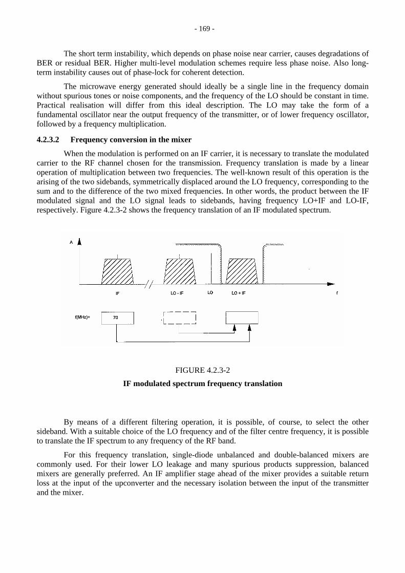
- 169 -

The short term instability, which depends on phase noise near carrier, causes degradations of BER or residual BER. Higher multi-level modulation schemes require less phase noise. Also long-term instability causes out of phase-lock for coherent detection.

The microwave energy generated should ideally be a single line in the frequency domain without spurious tones or noise components, and the frequency of the LO should be constant in time. Practical realisation will differ from this ideal description. The LO may take the form of a fundamental oscillator near the output frequency of the transmitter, or of lower frequency oscillator, followed by a frequency multiplication.

4.2.3.2 Frequency conversion in the mixer

When the modulation is performed on an IF carrier, it is necessary to translate the modulated carrier to the RF channel chosen for the transmission. Frequency translation is made by a linear operation of multiplication between two frequencies. The well-known result of this operation is the arising of the two sidebands, symmetrically displaced around the LO frequency, corresponding to the sum and to the difference of the two mixed frequencies. In other words, the product between the IF modulated signal and the LO signal leads to sidebands, having frequency LO+IF and LO-IF, respectively. Figure 4.2.3-2 shows the frequency translation of an IF modulated spectrum.

FIGURE 4.2.3-2

IF modulated spectrum frequency translation

By means of a different filtering operation, it is possible, of course, to select the other sideband. With a suitable choice of the LO frequency and of the filter centre frequency, it is possible to translate the IF spectrum to any frequency of the RF band.

For this frequency translation, single-diode unbalanced and double-balanced mixers are commonly used. For their lower LO leakage and many spurious products suppression, balanced mixers are generally preferred. An IF amplifier stage ahead of the mixer provides a suitable return loss at the input of the upconverter and the necessary isolation between the input of the transmitter and the mixer.

- 170 -

4.2.3.3 Transmission power versus peak factor and modulation format “(back-off)” with and without linearisation

For the design of the transmitter, two basic concepts are to be taken into consideration: modulation format and non-linearity of the IF and RF devices to be used.

When increasing the complexity of the modulation, the S/N ratio required (with the same BER) increases as well, therefore to maintain the system gain (in spite of the worse receive threshold), it is necessary to increase the transmitted power.

Every modulation format, with an average transmitted power, has a static peak factor, related to the possible states of the carrier.

Depending on the chosen roll-off to the static peak, it is necessary to add a dynamic peak, related to the carrier transition from one state to another. The transmission chain has to allow the dynamic of the carrier, without arriving at the gain saturation. Saturation and non-linearity may be described, in a vectorial way, as AM/AM and AM/PM (as described later), which give inter-symbol interference.

Transmitter non-linearity characterisation may be performed by means of an evaluation of the output spectrum when the inputs of the transmitter are two or more suitable tones. A direct evaluation, with the actual spectrum, is less precise, because the distortion inside the signal bandwidth cannot be evaluated.

4.2.3.4 Power amplifier

Available power at the output of an IF/RF converter is of the order of few milliwatt, and an amplification is therefore necessary for obtaining the required output level. Using GaAs FET (see Note 1) devices for the RF direct amplification is a common practice. Power transistors may be characterised by a parameter, P1 dB, that indicates the minimum output power at which the gain of the stage is 1 dB compressed. Therefore, a point of the transfer function is identified, near the saturation, when the device starts to compromise its linearity. From that point, a rapidly increasing amplitude distortion gives a degradation of BER for the signal containing a significant amount of amplitude modulation, like QAM modulation format.

NOTE 1 – Field effect transistor (FET) using Gallium Arsenide (GaAs).

To guarantee a suitable amount of linearity and for having low distortion, even in the presence of the amplitude peaks of the modulation, it is necessary to fix the output power (Pu) at a value less than P1 dB. The difference between these two values (Pb0 = P1 dB -Pu), is usually called an amplifier “back-off”. On the other hand, increasing the amount of back-off will increase the cost of the amplifier. Consequently, a small amount of residual distortion may be compensated for by techniques such as predistortion.

Figure 4.2.3-3 shows a typical non-linear characteristic of a high power amplifier and an operation point with a back-off. To specify the saturation level, 1 dB gain compression level (P1 dB) is generally used as reference point.

Typical back-off from P1 dB, together with typical roll-off factors, are shown in Table 4.2.3-1 for various modulation schemes.

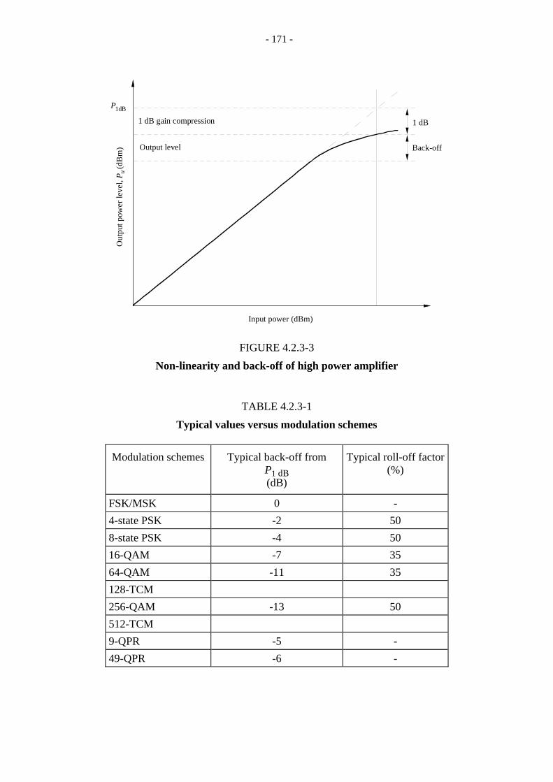
- 171 -

Input power (dBm)

1 dB gain compression

Output level

1 dB

Back-off

Out

put p

ower

leve

l, P

(dB

m)

u

1dBP

FIGURE 4.2.3-3

Non-linearity and back-off of high power amplifier

TABLE 4.2.3-1

Typical values versus modulation schemes

Modulation schemes Typical back-off from P1 dB (dB)

Typical roll-off factor (%)

FSK/MSK 0 -

4-state PSK -2 50

8-state PSK -4 50

16-QAM -7 35

64-QAM -11 35

128-TCM

256-QAM -13 50

512-TCM

9-QPR -5 -

49-QPR -6 -

- 172 -

Output power required by a transmitter of DRRS depends on many parameters such as bit rate, modulation formats, hop distance, fading probability, antenna gain etc.

For small capacity DRRS, thermal noise is the dominant factor and therefore an adequate output power level can increase the quality of a system.

Conversely, as the band increases, distortions become the main source of degradations and increasing of the output power may not be effective.

Adaptive Transmitter Power Control (ATPC) techniques can be used to reduce the output power during normal propagation conditions. This solution and its effects are described in § 4.3.4.

The effects of non-linearity are a displacement of the states of the modulated signal in the phase plane and the generation of intermodulation spectrum. A third-order non-linearity of an amplifier generates over the desired signal an intermodulation spectrum up to three times as wide as the original signal. This spreading, as shown in Fig. 4.2.3-4, can cause interference to the adjacent channel signals.

f0 + IFf

0– IFf0

Frequency

Originalspectrum

Additional spectrumgenerated by non-linearity

Am

plitu

de

FIGURE 4.2.3-4

Example of spectrum spreading due to non-linearities

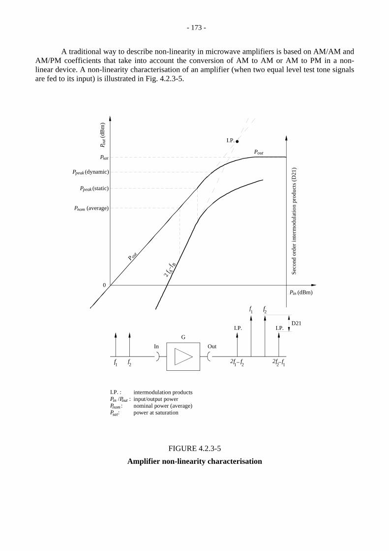
- 173 -

A traditional way to describe non-linearity in microwave amplifiers is based on AM/AM and AM/PM coefficients that take into account the conversion of AM to AM or AM to PM in a non-linear device. A non-linearity characterisation of an amplifier (when two equal level test tone signals are fed to its input) is illustrated in Fig. 4.2.3-5.

D21

P

(dB

m)

out

P sat

P (dynamic)peak

P (static)peak

P (average)nom

P out

0

P out

I.P.

G

In Out

1f 2f

I.P. I.P.

1f

2f

P (dBm)inSe

cond

ord

er in

term

odul

atio

n pr

oduc

ts (D

21)

2f

12f – 1

f2

2f –

–fB

2 f A

I.P. :P /P :P :P :

in outnom

sat

intermodulation productsinput/output powernominal power (average)power at saturation

FIGURE 4.2.3-5

Amplifier non-linearity characterisation

- 174 -

4.2.3.5 Spurious emissions (types and requirements) (internal/external)

Spurious emissions are defined as emissions at frequencies which are outside the necessary bandwidth, as defined in § 3.4.5. The level of these emissions may (and should be) reduced without affecting the corresponding transmission of information.

Spurious emissions include harmonic and parasitic emissions, intermodulation products and frequency conversion products, while emissions resulting from the modulation process are excluded.

Spurious emission limits from transmitter shall be defined for two reasons: to limit interference into systems operating wholly externally to the considered system channel plan and to limit local interference within the considered system where transmitters and receivers are directly connected via filter and branching system.

This leads to two sets of spurious emission limits, where the specific limits given for internal interference shall be no greater than the external level limits at point B' for indoor systems and C' for outdoor systems where a common Tx/Rx duplexer is used (see Fig. 4.2.3-1).

4.2.3.6 Linearisation (requirements and techniques)

The first countermeasure for linearisation is to operate the amplifier sufficiently backed off from its saturation point to prevent signal peaks from becoming saturated.

With high order modulation formats, a predistortion technique may be used to improve linearity of the amplifier. The concept at the base of the different predistortion realisations (in BB or at IF or at RF) is to put somewhere in the amplifier chain some degree of non-linearity for compensating amplifier non-linearity.

These non-linearities typically show two effects:

– non-linearity between input power and output power, called AM/AM conversion;

– output phase variation, in non-linear relation with input power, called AM/PM conversion.

Consequently, the predistorter circuit has characteristics of amplitude-power and phase-power to compensate those of the amplifier.

Predistortion may be performed:

– in a path parallel to the signal, with independent generation and adjustment of phase and amplitude, and subsequent sum to signal itself (as shown in Fig. 4.2.3-6); this operation is generally performed at IF;

– along the signal path, using devices with gain expansion (AM/AM control) and phase modulation (AM/PM control) capabilities, equal and opposite to those of subsequent devices (as shown in Fig. 4.2.3-7); this operation is generally performed at RF.

The effect of the predistortion on the third order intermodulation is shown in Fig. 4.2.3-8.

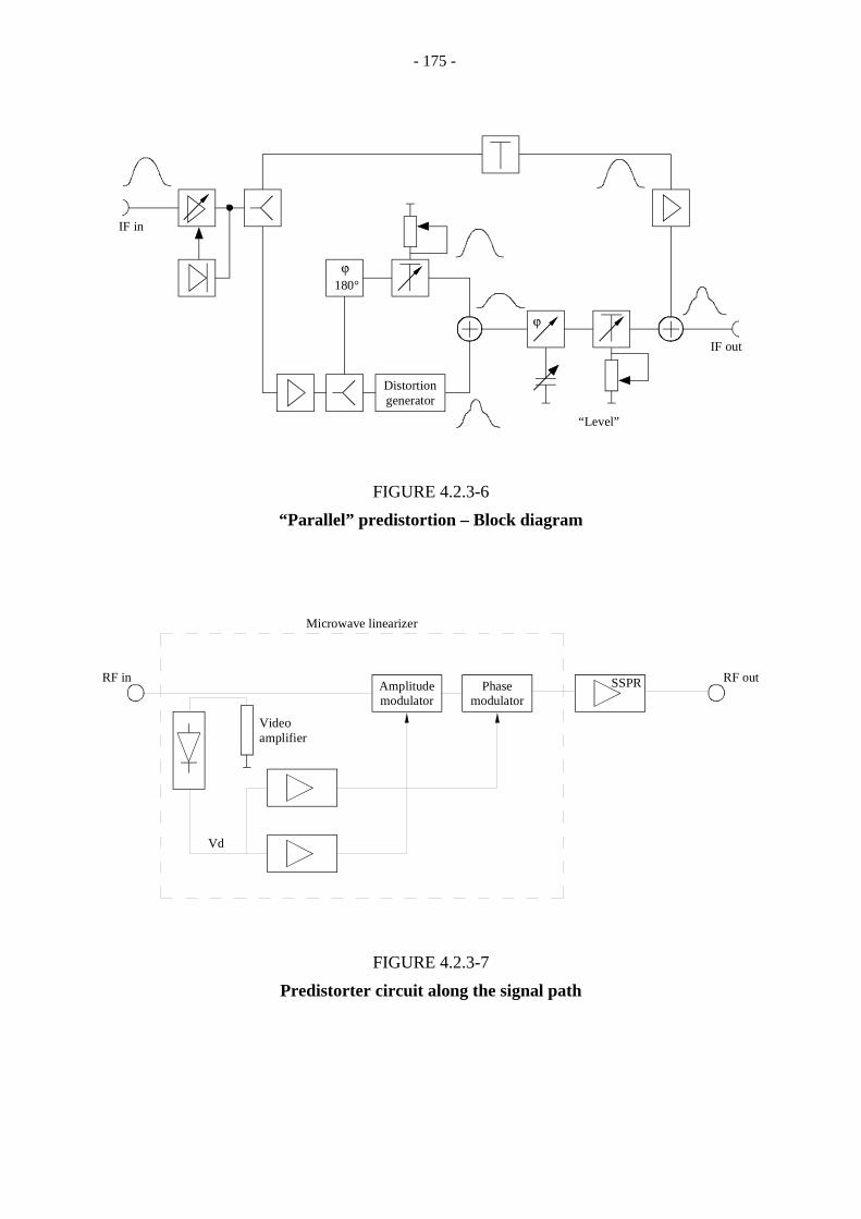
- 175 -

ϕ

ϕ180°

Distortiongenerator

“Level”

IF out

IF in

FIGURE 4.2.3-6

“Parallel” predistortion – Block diagram

RF in RF outAmplitudemodulator

Phasemodulator

SSPR

Vd

Videoamplifier

Microwave linearizer

FIGURE 4.2.3-7

Predistorter circuit along the signal path

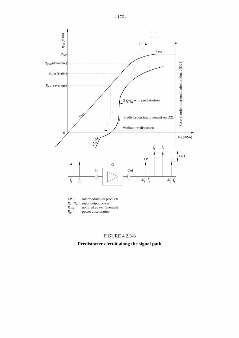
- 176 -

D21

P

(dB

m)

out

P sat

P (dynamic)peak

P (static)peak

P (average)nom

P out

0

P out

I.P.

G

In Out

1f

2f

I.P. I.P.

1f

2f

P (dBm)in

Seco

nd o

rder

inte

rmod

ulat

ion

prod

ucts

(D21

)

I.P. :P /P :P :P :

in outnom

sat

intermodulation productsinput/output powernominal power (average)power at saturation

2f

12f – 1f2

2f –

–fB

2 f A

Without predistortion

Predistortion improvement on D21

with predistortion–fB 2 fA

FIGURE 4.2.3-8

Predistorter circuit along the signal path

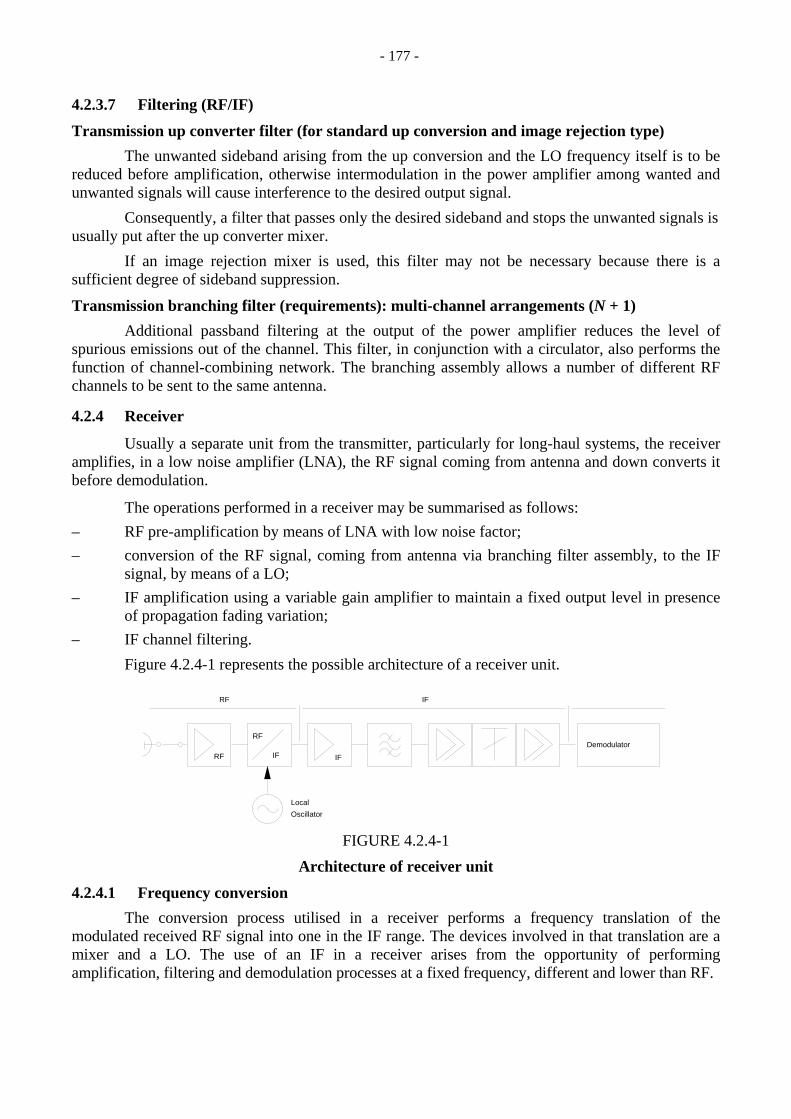
- 177 -

4.2.3.7 Filtering (RF/IF)

Transmission up converter filter (for standard up conversion and image rejection type)

The unwanted sideband arising from the up conversion and the LO frequency itself is to be reduced before amplification, otherwise intermodulation in the power amplifier among wanted and unwanted signals will cause interference to the desired output signal.

Consequently, a filter that passes only the desired sideband and stops the unwanted signals is usually put after the up converter mixer.

If an image rejection mixer is used, this filter may not be necessary because there is a sufficient degree of sideband suppression.

Transmission branching filter (requirements): multi-channel arrangements (N + 1)

Additional passband filtering at the output of the power amplifier reduces the level of spurious emissions out of the channel. This filter, in conjunction with a circulator, also performs the function of channel-combining network. The branching assembly allows a number of different RF channels to be sent to the same antenna.

4.2.4 Receiver

Usually a separate unit from the transmitter, particularly for long-haul systems, the receiver amplifies, in a low noise amplifier (LNA), the RF signal coming from antenna and down converts it before demodulation.

The operations performed in a receiver may be summarised as follows: – RF pre-amplification by means of LNA with low noise factor; – conversion of the RF signal, coming from antenna via branching filter assembly, to the IF

signal, by means of a LO; – IF amplification using a variable gain amplifier to maintain a fixed output level in presence

of propagation fading variation; – IF channel filtering.

Figure 4.2.4-1 represents the possible architecture of a receiver unit.

RF IF

RF

IFDemodulator

OscillatorLocal

RF IF

FIGURE 4.2.4-1

Architecture of receiver unit

4.2.4.1 Frequency conversion

The conversion process utilised in a receiver performs a frequency translation of the modulated received RF signal into one in the IF range. The devices involved in that translation are a mixer and a LO. The use of an IF in a receiver arises from the opportunity of performing amplification, filtering and demodulation processes at a fixed frequency, different and lower than RF.

- 178 -

Frequency translation, performed by a linear operation of multiplication between the two frequencies, generates two sidebands, symmetrically displaced around the LO frequency, corresponding to the sum and to the difference of the two mixed frequencies. The product between the RF modulated signal and the LO signal leads to sidebands, having frequency RF + LO and RF – LO, respectively. Figure 4.2.4-2 shows the frequency translation of an RF modulated spectrum.

70f (MHz) =

Am

plitu

de, A

Frequency, f

RF – IF = LO LO – IF LO RF RE + LO

FIGURE 4.2.4-2

RF modulated spectrum translation

An RF filter plays the important role of suppressing the image frequency, that is the frequency value (LO – IF) symmetrically displaced with respect to LO. With a suitable choice of the LO frequency, it is possible to translate any RF frequency into one IF signal.

4.2.4.2 Filtering

A number of general considerations about filtering are listed below: – RF filter, typically part of a branching assembly, eliminates the unwanted signals and has a

moderate influence in eliminating adjacent channel interference. – IF filter is the so-called channel filter which gives a better selectivity to the adjacent

channels, avoiding possible saturation of the demodulator. – Baseband receiving filter is the post-demodulation filter, which limits the noise bandwidth

and gives the proper shape to the received pulses; it makes the major contribution to suppressing the adjacent channel interference.

– NFD (net filter discrimination) (or IRF, interference reduction factor) is a ratio (dB) related to the transmitted spectrum type and to the filtering process in the receiver. It expresses the residual portion of an interference spectrum (at a certain distance from the received RF signal), which can reach the decision point of the demodulator. NFD is a useful parameter to convert the effects of out-of-band interferences to an equivalent effect, due to a co-channel interference.

- 179 -

Reception branching filter

Branching assembly is a common way to feed a number of receivers, working at different frequencies, with the broadband signal coming from a common antenna system. Typically, the building blocks of a branching assembly are circulators and channel filters.

The passband type channel filters are tuned at the carrier frequencies of the receivers and play the important role of attenuating the image frequencies, avoiding its conversion to the IF signal, and attenuating other unwanted out-of-band signals as well. Moreover, they present, at their input port, a negligible impedance for frequencies external to their passband frequency, reflecting them back.

Multi-channel arrangement (N + 1)

Figure 4.2.4-3 represents an example of the architecture of a multi-channel arrangement.

feeder

Tx Rx

1 1 3 1 13 3 1 3 3

2 2

2

2 2

Ft1 Ft2 Fr1 Fr1

Tx1 Tx2 Rx1 Rx2

FIGURE 4.2.4-3

Multi-channel arrangement layout

Low noise amplifier image filter techniques

After the RF filter stage, generally the first operation performed in a receiver is low noise preamplification, often integrated into the same unit with the mixer. Protection against up fading propagation may be provided by an AGC controlled variable gain stage.

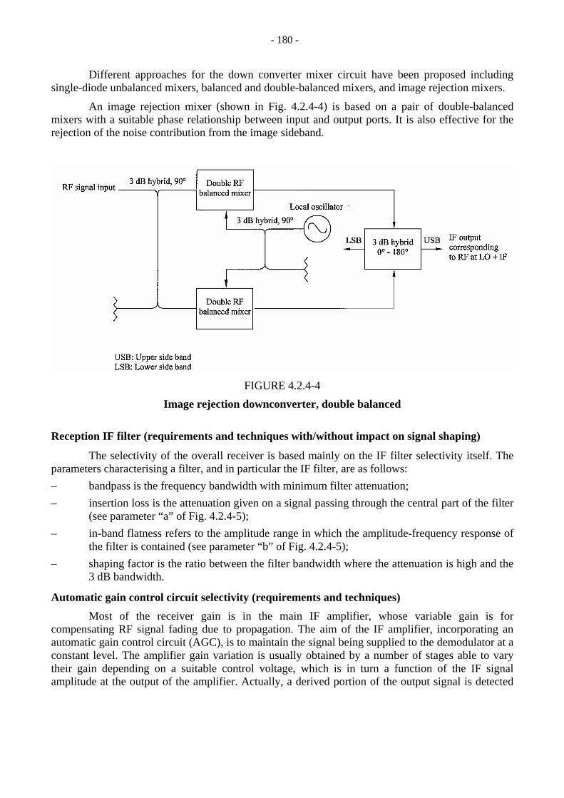
- 180 -

Different approaches for the down converter mixer circuit have been proposed including single-diode unbalanced mixers, balanced and double-balanced mixers, and image rejection mixers.

An image rejection mixer (shown in Fig. 4.2.4-4) is based on a pair of double-balanced mixers with a suitable phase relationship between input and output ports. It is also effective for the rejection of the noise contribution from the image sideband.

FIGURE 4.2.4-4

Image rejection downconverter, double balanced

Reception IF filter (requirements and techniques with/without impact on signal shaping)

The selectivity of the overall receiver is based mainly on the IF filter selectivity itself. The parameters characterising a filter, and in particular the IF filter, are as follows: – bandpass is the frequency bandwidth with minimum filter attenuation; – insertion loss is the attenuation given on a signal passing through the central part of the filter

(see parameter “a” of Fig. 4.2.4-5); – in-band flatness refers to the amplitude range in which the amplitude-frequency response of

the filter is contained (see parameter “b” of Fig. 4.2.4-5); – shaping factor is the ratio between the filter bandwidth where the attenuation is high and the

3 dB bandwidth.

Automatic gain control circuit selectivity (requirements and techniques)

Most of the receiver gain is in the main IF amplifier, whose variable gain is for compensating RF signal fading due to propagation. The aim of the IF amplifier, incorporating an automatic gain control circuit (AGC), is to maintain the signal being supplied to the demodulator at a constant level. The amplifier gain variation is usually obtained by a number of stages able to vary their gain depending on a suitable control voltage, which is in turn a function of the IF signal amplitude at the output of the amplifier. Actually, a derived portion of the output signal is detected

- 181 -

by a diode, filtered by an AGC filter (which prevents signals external to the wanted spectrum from influencing the overall response of the amplifier), amplified and then used as control voltage for the variable gain stages. This way, a feedback path from the output and the intermediate stages allows for compensating input level variation with a variable gain and for maintaining constant IF output level.

50200– 10– 20– 30– 40– 50 10 30 40

– 10

– 20

– 30

– 40

– 50

– 60

– 70

0

ba

x1x1

x2x2

x3 x3

Atte

nuat

ion

(dB

)

Frequency (MHz)

FIGURE 4.2.4-5

IF filter selectivity example

Baseband filters

(See Spectrum shaping - § 4.2.2.5.)

4.2.4.3 Noise figure

The noise figure represents the general formula and criteria of the addition of different components.

The noise figure is defined, in linear terms, as follow:

F = (S/N)in / (S/N)out with T = 290 K (4.2.4-1) where:

(S/N)in : signal-to-noise ratio at the input of the system or of the device under consideration

(S/N)out : signal-to-noise ratio at the output

T : temperature of the system.

Noise figure is usually given in dB: F (dB) = 10 log F (4.2.4-2)

- 182 -

The noise figure value of an individual device allows determination of the noise figure of a cascade of devices by the following:

Ftotal = F1 + (F2 - 1)/G1 +........+ (Fn - 1)/(G1G2... Gn - 1) (4.2.4-3) where:

Ftotal : overall system noise figure Fi and Gi : noise figure, and gain, respectively, of the i-th individual device i : integer between 1 and n.

Many contributions can degrade the receiver noise figure, including losses of filter and circuit, subsequent stages noise, and isolators used to enhance return loss values required by broadband communication equipments.

If the overall system noise figure is too high, the capability of the receiver to process low level or weak signals is greatly reduced.

4.2.4.4 Required bandwidth

(See § 4.2.3.7 – Filtering (RF/IF).)

4.2.4.5 Signature

(See § 4.3 – Countermeasures.)

4.2.5 Radio protection switching

4.2.5.1 General

High availability is very important for a radio-relay system (see § 3.2.3).

In order to achieve the availability objective, it is necessary to provide some kind of redundant equipment in a digital radio-relay system so that the service can be restored when normal equipment fails.

Moreover the protection channel can improve the quality of performance since multipath fading is a frequency selective phenomena and a significant uncorrelation of fading events on different RF carriers has been observed in several propagation experiments.

4.2.5.2 Types of protection arrangements

Single route systems may be protected in one of four ways: – protection switching on a set stand-by basis, – multi-line switching with a dedicated protection channel, – space diversity operation (see § 4.3.6), – polarization, angle and pattern diversity operation (see § 4.3.7).

In theory, the switch may operate at RF, IF or baseband, but in practice, baseband switching is preferred in case of multi-line switching, since this may protect the complete channel from input port to output port with a minimum duplication of equipment outside the switched path.

Dual route diversity protection facilitates the use of greater hop lengths in frequency bands where attenuation due to precipitation plays the key role on availability. Switching from “Route-1-link” to “Route-2-link” is accomplished at the terminal receiver. It may be necessary to equalize the difference in transmission time between the path lengths of each route, in order that the signal on both routes may be aligned at the instant of changeover.

- 183 -

In the case of radio systems used for local access, such redundant equipment may be dispensed with from the economical point of view.

4.2.5.3 Architecture of radio protection switching

With digital transmission, a variation in the number of bits between the frame alignment signals results in loss of alignment in the following demultiplexer, and transmission is interrupted until the demultiplexer has regained alignment. On radio-relay links, fading initially causes a deterioration in transmission quality leading eventually to an interruption. If a high-speed quality monitor were used to switch, without a slip in bit count, to a better protection channel before the signal is interrupted, it would be possible to avoid an interruption altogether.

In order to operate as a countermeasure against multipath fading, the switching system must operate in a truly “error free hitless” mode, preserving the “bit count integrity” of the output bit stream, and the overall switching time must be short enough to counteract fast fading events.

In order to operate “error free” switching and to maintain the “bit count integrity” even in the case of severe multipath fading, two fundamental requirements must be fulfilled: – The switching system must compensate for the different and time-varying transmission

delays on the working channel and on the protection channel: a fast delay adjustment procedure is required before switching.

– The overall switching sequence must be completed before the “outage BER” threshold (BER = 10-3) is reached.

Hitless switch

A functional block diagram of hitless switch is shown in Fig. 4.2.5-1. When fading occurs in the working channel and the quality threshold is exceeded, the distributor at the transmitting end bridges the protection channel to the channel affected.

The same signal is then present at both inputs of hitless switch (HL SW) in the degraded working channel and an alignment procedure can commence.

After the two signals have been aligned, it is possible to switch (select) from the working to the protection channel in a completely error free mode.

As restoral from the protection channel to the working channel is effected in the same way, it is also hitless.

FIGURE 4.2.5-1

Function block diagram of hitless switch

- 184 -

4.2.5.4 Protection switching on set stand-by basis

This is a simple arrangement for protection switching. At each radio station, one receiver, one transmitter or one transmitter/receiver has a stand-by equipment, generally on a cold stand-by basis. Here, “cold” means that the stand-by equipment is usually switched off.

Protection switching on set stand-by basis is suitable for a radio-relay system which is comprised of one working radio channel and, at most, two working radio channels. This scheme has an advantage from the spectrum management viewpoint that no additional radio frequency is necessary for protection.

However, when there are more working channels, the set stand-by protection becomes unjustified from the economical point of view and, therefore, the multi-line switching should be preferred.

4.2.5.5 Multi-line switching

In case of multi-line switching (e.g. using frequency diversity, see § 4.3.9), one or P (P > 1) protection radio channels are prepared for N working channels. When one of the N working channels is interrupted, the signal in the interrupted channel will immediately be recovered by one of the protection channels over m radio hops. In such a case, the unavailability U in one switching section of each both-way radio channels due only to equipment failure, assuming that the failure rate of switching equipments is negligibly small, can be expressed by the following formula:

UN

N PP

mq P=++

⎛⎝⎜

⎞⎠⎟ +2

11( ) (4.2.5-1)

where: m: number of radio hops contained in a switching section q: probability of an interruption of each hop (as far as equipment failure is concerned,

q = MTTR/MTBF, where MTTR is mean time to repair and MTBF is mean time between failures)

and:

N PP

N PP N

++

⎛⎝⎜

⎞⎠⎟ =

++ −1 1 1( )!

( )!( ) (4.2.5-2)

Formula (4.2.5-1) can be derived from the following considerations under the assumption that q is sufficiently small. The probability of a failure of one radio channel (working or protection) in a switching section is mq. The probability of a failure of a specific set of P + 1 radio channels is (mq)P + 1. The value of formula (4.2.5-2) gives the number of combinations of finding P + 1 radio channels out of N + P radio channels. In such a situation, one of the working radio channels fails because the protection channels cannot recover it. Therefore, the value is divided by N. Finally, the factor 2 is multiplied because a failure in one of the two directions causes unavailability.

In many cases the number of protection channels P = 1 and formula (4.2.5-1) can be written as follows:

U N mq= +( )( )1 2 (4.2.5-3)

- 185 -

In rare cases, P = 2 may be chosen for a radio-relay route which traverses over an area difficult to access and formula (4.2.5-1) can be written as follows:

U N N mq= + +13

2 1 3( ) ( ) ( ) (4.2.5-4)

Protection switching is effective not only for equipment failures but also for multipath fading through frequency diversity effects. Information on frequency diversity is given in § 4.3.9.

As an example, assume that the allowable unavailability due to radio equipment failure is 1

3

of the overall unavailability. In this case, assuming a switching section of 280 km length, the allowable value of U is 0.00011, according to Recommendation ITU-R F.695. Further assuming N = 7 and m = 6, in case of one protection channel, from formula (4.2.5-3), we can derive q = 0.00062.

This means that if MTBF is 10 000 h, MTTR of 6.2 h is allowed and that if MTBF is 30 000 h, MTTR of 18.6 h is allowed.

Modern digital radio equipment show a large value of MTBF generally in the order of several tens of thousands of hours. Therefore, radio-relay systems can demonstrate a very high availability.

At the same time, it should be noted that the actual values of the system availability depend very much on the values of MTTR, which are determined by the maintenance organization. Well trained maintenance personnel and a good maintenance organization are key factors for high system availability.

It should also be noted that power supply failure and precipitation attenuation (in particular for frequencies above about 10 GHz) are also important factors in availability considerations, and that multi-line switching is not effective for these factors.

4.2.5.6 Factors influencing the choice of switching criteria

The switching criteria are influenced by the main role of the protection switching.

If switching is used to improve performance during poor propagation conditions, this would require the rapid recognition of switching criteria and it is desirable to switch to a stand-by channel without loss of synchronization. This also facilitates preventive maintenance operations. It should be noted that the addition or loss of bit, due for instance to switching without prior arrangements to ensure coincidence or to a spurious impulse affecting the timing, may completely desynchronize the downstream transmission chain and cannot be considered an isolated error. To realize this, the “hitless switching” should be utilized with suitable switching criteria.

Digital radio-relay systems use a radio-relay frame inserted at the terminal station for monitoring purposes. The frame alignment signal and a parity bit (and/or a syndrome bit) are used to monitor interruptions and quality, respectively.

The monitoring criteria are generated in the radio equipment. When the system judges circuit interruption, such signal is sent to the switchover control equipment for protection switch operation.

- 186 -

If the transmission quality is degraded, the quality alarm (BER alarm) is initiated. The alarm threshold can be matched to the characteristics of the link. Usually, a BER of 10-6 is predetermined as an alarm threshold.

4.2.5.7 Calculation of link unavailability

As the individual causes of unavailability are statistically independent, then the overall link unavailability is calculated by summing the unavailability due to the independent causes. The calculated link unavailability can then be compared with the availability objective to determine if the predicted link availability is satisfactory.

Often one of the causes of unavailability is significantly larger than the others and this cause will then dominate the overall link availability. In this case, it will be most economic to try to economically reduce the largest cause of unavailability, rather than improving the minor causes of unavailability. If equipment unavailability of unprotected equipment is the dominant cause of not satisfying the link availability objective, then equipment redundancy (duplication and/or N + 1 protection switching) will need to be provided.

4.2.6 Antennas and feeder systems

4.2.6.1 Fundamentals of radio-relay antennas

In radio-relay systems, the repeater distance is typically in the range of 40 to 50 km because of path clearance and fading, even if antennas are installed on towers. Furthermore, when the systems are operating at frequencies higher than 10 GHz, antennas are often necessary at every few km because the radio wave may be attenuated by rain and other precipitation. Thus, the antennas must have high efficiency and economical cost.

Some radio-relay routes require more than several tens of thousands of channels of communication capacity. In this case, antennas are required to have a wide band capability to transmit and receive radio signals in multiple frequency bands. Further, when the dual orthogonal polarizations at the same radio frequency are utilized to increase the communication capacity, antennas must have high cross-polarization discrimination (XPD).

As radio-relay networks become dense and the number of routes operating in the same frequency bands increases, the interference between routes will also increase. To suppress the interference, antennas must have good radiation patterns including good wide-angle sidelobe levels.

Gain and radiation patterns

The directivity or directive gain Gd is defined as follows:

GE r

E r d dd

P

P=

∫∫

4 2

002 2

π

θ θ ϕππ

( )

( ) sin (4.2.6-1)

where Ep(r) is the radiated field. Therefore, Gd is a function of θ (off-axis angle) and ϕ (rotational angle from the horizontal plane), independent of r (distance). The maximum value of Gd is called directive gain of the antenna when the direction is not specified.

The power gain G is defined as:

G = ηr Gd (4.2.6-2)

where ηr, radiation efficiency, is the ratio of the power radiated from an antenna to the power accepted at its input terminal from the power source and corresponds to the dissipation loss of the antenna.

- 187 -

When the actual area of the antenna aperture is designated by A, the directivity Gd is given by:

Gd = (4π/λ2)A ηa (4.2.6-3)

where ηa is the aperture efficiency and λ is the wavelength in free space.

The e.i.r.p. is the product of the power gain Gt in a given direction of a transmit antenna and the power Pt transmitted by the antenna from the power source. When two antennas, transmitting and receiving, face each other with distance r, the received power Pr of the receive antenna with gain Gr is:

Pr = (e.i.r.p.)⋅Gr/Ls (4.2.6-4)

where:

e.i.r.p. = Pt⋅Gt

Ls = (4πr/λ)2

and Ls is called free-space loss and r is the hop distance [Kitsuregawa, 1990].

The radiation pattern of an antenna is the spatial distribution of a quantity such as amplitude, phase, polarization, or power flux-density of the radiated field. The radiation pattern of the antenna used for radio-relay system is often a pencil-beam pattern which has a single, relatively narrow beam. A typical amplitude pattern of a pencil-beam antenna is characterized by a main lobe, sidelobes, nulls, and half-power beamwidth as shown in Fig. 4.2.6-1 [Kitsuregawa, 1990].

0 dB

Half-powerbeamwidth

– 3 dB

Side lobe level (dB)

Side lobes (dB)

Back lobe (dB)

Main lobe

0°– 180° 180°Nulls

Off-axis angle (degrees)

Am

plitu

de (d

B)

FIGURE 4.2.6-1

Terms associated with radiation patterns

- 188 -

Recommendation ITU-R F.699 gives the radio-relay antenna characteristics used for interference assessment between line-of-sight radio-relay systems or coordination studies and interference assessment between line-of-sight radio-relay stations and stations in space radiocommunication services sharing the same frequency band and presents the following reference radiation pattern for radio-relay antennas operating at frequencies between 1 GHz and 40 GHz. It should be noted that the radiation pattern of an actual antenna may be worse than the reference radiation pattern over a certain range of angles. Therefore, the reference radiation pattern in this Recommendation should not be interpreted as establishing the maximum limit for radiation patterns of existing or planned radio-relay system antennas.

a) If D/λ is greater than 100:

( )G GD

maxθλ

θ= − × ⎛⎝⎜

⎞⎠⎟

−2 5 10 32

. for 0 ≤ θ <θm (4.2.6-5)

G (θ) = G1 for θm ≤ θ < θr (4.2.6-5)

G (θ) = 32 – 25 log θ for θr ≤ θ < 48° (4.2.6-5)

G (θ) = – 10 for 48° ≤ θ ≤ 180° (4.2.6-5)

where:

D : antenna diameter

λ : wavelength ⎪⎭

⎪⎬⎫

expressed in the same unit

θ : off-axis angle

Gmax : main lobe antenna gain = 7.7 + 20 log (D/λ) (dB)

G1 : gain of first sidelobe = 2 + 15 log (D/λ) (dB)

θλ

m maxDG G= −20 1 (degrees)

θr = 15.85(D/λ)-0.6 (degrees)

b) If D/λ is less than 100

( )G GD

maxθλ

θ= − × ⎛⎝⎜

⎞⎠⎟

−2.5 10 32

for 0 ≤ θ < θm (4.2.6-6)

G (θ) = G1 for θm ≤ θ < 100 (λ/D) (4.2.6-6)

G (θ) = 52 – 10 log (D/λ) – 25 log θ for 100 (λ/D) ≤ θ < 48° (4.2.6-6)

G (θ) = 10 – 10 log (D/λ) for 48° ≤ θ < 180 ° (4.2.6-6)

Polarization

Polarization of a wave radiated by an antenna is expressed by the shape and motion of the locus of the extremity of the time-varying electric field vector at a fixed point. A wave having an electric field vector with its extremity describing a straight line segment as a function of time is

- 189 -

called a linearly polarized wave. When the extremity of field vector describes a circle or an ellipse as a function of time, the wave is called circularly polarized wave or elliptically polarized wave. If this rotates clockwise (or counterclockwise) looking in the direction of propagation, the sense of polarization is said to be right-handed (or left-handed).

If the locus of field vector is plotted, a polarization ellipse will generally be obtained as shown in Fig. 4.2.6-2 [Kitsuregawa, 1990]. Parameters characterizing the elliptical polarization are sense of polarization, axial ratio, and tilt angle. The polarization that the antenna is intended to radiate or receive is called co-polarization. Cross-polarization is the polarization orthogonal to the co-polarization. If the state of polarization of a receive antenna is not adjusted for a maximum received power, loss occurs due to polarization mismatch. This loss corresponds to polarization efficiency or the polarization mismatch factor.

Tilt angle

Reference axis

Minor axis

Major axis

Sense of polarization

E

z

x

y

τ

Direction of propagation: z-axis

Axial ratio Length of major axisLength of minor axis=

Ex

Ey

FIGURE 4.2.6-2

Polarization ellipse

- 190 -

4.2.6.2 Parabolic antenna

A parabolic antenna consists of a paraboloidal reflector and a primary radiator with its phase centre at the focus of the paraboloidal reflector as shown in Fig. 4.2.6-3. The parabolic antenna is very practical because of its good electrical characteristics and its simple structure with low cost.

x

yz

F0

D

θ θaPrimary horn

Parabolic reflector

r

FIGURE 4.2.6-3

Parabolic antenna

The subtended angle of the reflector is usually selected to be between 140° and 180°. The larger the subtended angle, the better the wide-angle radiation pattern but less the aperture efficiency ηa. Aperture efficiency ηa is decreased by the aperture distribution of the field on the reflector, spillover loss, blocking effects of primary radiator and its support strut, alignment error, surface error of the reflector and so on, and is usually between 50% and 60%. The value of Gmax given in § 4.2.6.1 assumes an aperture efficiency of 60%.

Dipole antennas, pyramidal horns or conical horns are used as the primary radiator, taking into account frequency, polarization, desired radiation pattern and so on.

Figure 4.2.6-4 shows an example of a parabolic antenna applied to the 6 GHz band radio-relay system. The aperture diameter is 4 m, the bandwidth is 500 MHz and orthogonal dual polarizations are used. Antenna gain is 45.5 dB, aperture efficiency 53%, XPD better than 38 dB and Voltage Standing Wave Ratio (VSWR) better than 1.05. Figure 4.2.6-5 shows the measured radiation patterns.

Cylindrical metal shields as shown in Fig. 4.2.6-6 are often attached to the reflector rim to improve the radiation pattern performance. Microwave absorbers are placed at critical locations inside the shield to reduce unwanted side and back lobes. Figure 4.2.6-7 shows the radiation patterns of a 2 GHz band antenna of 4 m diameter with and without absorbers. As shown in the figure, the absorbers reduce the unwanted sidelobes by more than 10 dB.

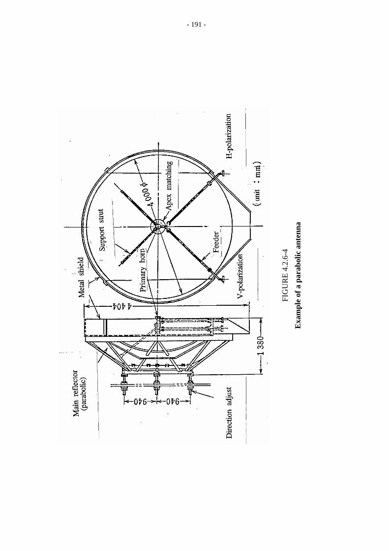
FIG

UR

E 4

.2.6

-4

Exa

mpl

e of

a p

arab

olic

ant

enna

- 191 -

- 192 -

FIGURE 4.2.6-5

Measured radiation patterns

FIGURE 4.2.6-6

Cylindrical metal shield

- 193 -

FIGURE 4.2.6-7

Radiation patterns with and without absorbers

4.2.6.3 Horn reflector antenna

A horn reflector antenna consists of a paraboloidal reflector and a primary radiator close to the reflector as shown in Fig. 4.2.6-8. The feed horn of the antenna is very large in comparison with wavelength, so the horn reflector antenna can be used for wide frequency bands. Further, the antenna has good VSWR characteristics and good radiation patterns in the horizontal plane because of no blockage at the aperture. In addition, the aperture efficiency ηa is high because the field distribution on the aperture is close to uniform. On the other hand, the antenna has disadvantages, such as large volume, heavy weight and high cost. So, the horn reflector antennas have been in wide use in the radio-relay routes where multiple frequency bands are used and the interference conditions are stringent. This type of antenna is generally being replaced by a new type such as shown in the next section.

FIGURE 4.2.6-8

Horn reflector antenna

- 194 -

4.2.6.4 High performance antenna

The combination of route congestion and the conversion from analogue to digital systems in radio-relay links in the 4 to 6 GHz range has given rise to the need for antennas with excellent wide-angle radiation patterns and superior cross-polarization characteristics. Therefore, the antenna must be capable of reducing inter-route and cross-polarization interference below the levels achievable by existing horn-reflector antennas. Further, in digital radio-relay systems, space diversity systems are required in more hops than in analogue systems to overcome multipath fading. So, a small sized and light weight antenna is required to decrease antenna load to towers and antenna set-up space on platforms.

A tri-reflector offset antenna consists of a corrugated conical horn as the primary radiator and the reflector system with three offset reflectors as shown in Fig. 4.2.6-9. The corrugated conical horn has only a small cross-polarization component and the reflector system is constructed so as to ensure that the cross-polarization components generated by the reflectors cancel out, thereby reducing the net cross-polarization component of the antenna.

FIGURE 4.2.6-9

Tri-reflector offset antenna

- 195 -

In case an antenna eliminating cross-polarized component based on geometrical optics is used in lower frequency band, cross-polarized components due to the asymmetry of reflectors remain because field distributions differ from those calculated based on geometrical optics. Beam mode analysis taking account of the change of field distributions due to frequency is applied to the design of tri-reflector type offset antenna.

The wide-angle radiation characteristics of an antenna for use in radio-relay links are especially important for prevention of interference in the horizontal plane, but not so much in the other plane. The sub and main reflectors are therefore shaped so as to obtain the aperture distribution with a low sidelobe type in the horizontal plane and high efficiency type in the elevation plane. As a result, it is possible to realize excellent wide-angle radiation patterns in the horizontal plane while preserving high aperture efficiency.

Figure 4.2.6-10 shows an example of a tri-reflector antenna with a 3.6 m aperture diameter applied to the 4/5/6 GHz bands radio-relay system. The height is about 5.6 m and the weight is about 1.6 t. The shape of the shielding plates are optimized and microwave absorbers, made of rubber and carbon, are attached at critical locations inside the shielding plates to reduce side and back lobes. Thin Fibre Reinforced Plastic (FRP) plates are attached across the opening of the shielding plates with an airtight seal, and the inside of antennas should be pressurized by dry air. The aperture efficiency is more than 59% , the peak level of cross-polarization radiation pattern is less than -40 dB below the peak level of co-polarization one and VSWR in the 4 to 6 GHz range is better than 1.035. Figure 4.2.6-11 shows the measured radiation patterns. The radiation level in the range of angle beyond 30° is less than -23 dBi.

FIGURE 4.2.6-10

Example of a tri-reflector antenna

FI

GU

RE

4.2

.6-1

1

Mea

sure

d ra

diat

ion

patt

erns

- 196 -

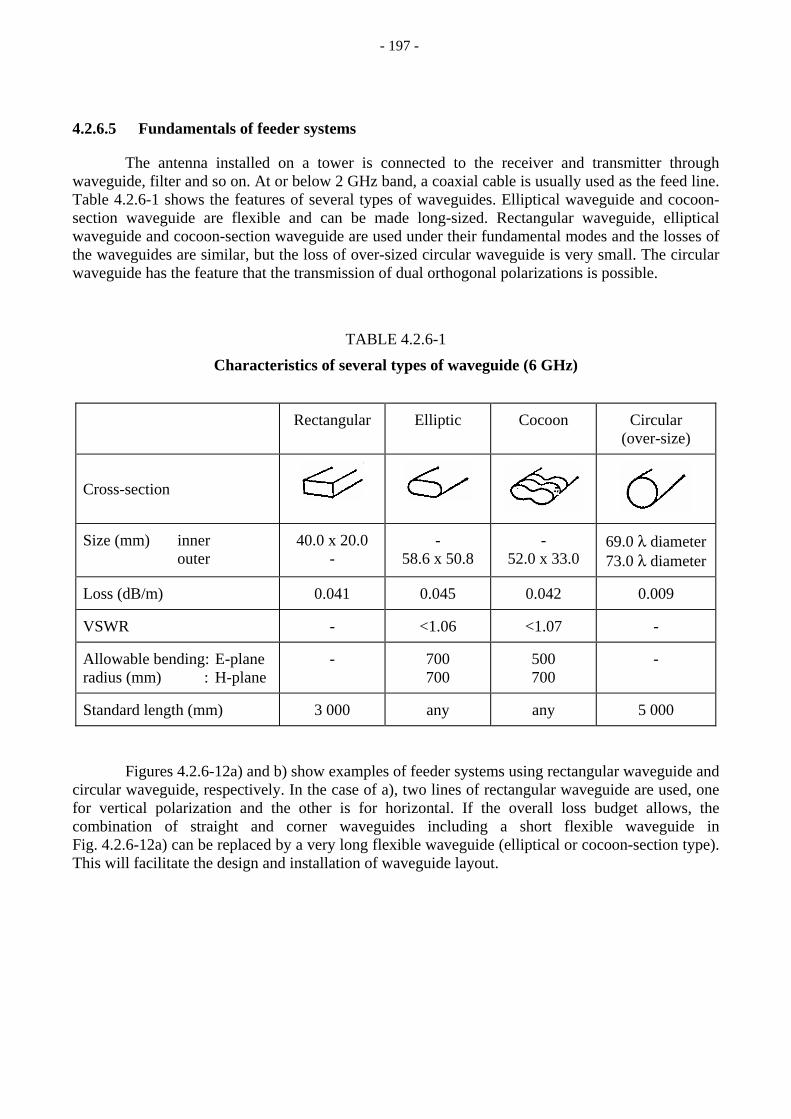
- 197 -

4.2.6.5 Fundamentals of feeder systems

The antenna installed on a tower is connected to the receiver and transmitter through waveguide, filter and so on. At or below 2 GHz band, a coaxial cable is usually used as the feed line. Table 4.2.6-1 shows the features of several types of waveguides. Elliptical waveguide and cocoon-section waveguide are flexible and can be made long-sized. Rectangular waveguide, elliptical waveguide and cocoon-section waveguide are used under their fundamental modes and the losses of the waveguides are similar, but the loss of over-sized circular waveguide is very small. The circular waveguide has the feature that the transmission of dual orthogonal polarizations is possible.

TABLE 4.2.6-1

Characteristics of several types of waveguide (6 GHz)

Rectangular Elliptic Cocoon Circular (over-size)

Cross-section

Size (mm) inner outer

40.0 x 20.0 -

- 58.6 x 50.8

- 52.0 x 33.0

69.0 λ diameter73.0 λ diameter

Loss (dB/m) 0.041 0.045 0.042 0.009

VSWR - <1.06 <1.07 -

Allowable bending: E-plane radius (mm) : H-plane

- 700 700

500 700

-

Standard length (mm) 3 000 any any 5 000

Figures 4.2.6-12a) and b) show examples of feeder systems using rectangular waveguide and circular waveguide, respectively. In the case of a), two lines of rectangular waveguide are used, one for vertical polarization and the other is for horizontal. If the overall loss budget allows, the combination of straight and corner waveguides including a short flexible waveguide in Fig. 4.2.6-12a) can be replaced by a very long flexible waveguide (elliptical or cocoon-section type). This will facilitate the design and installation of waveguide layout.

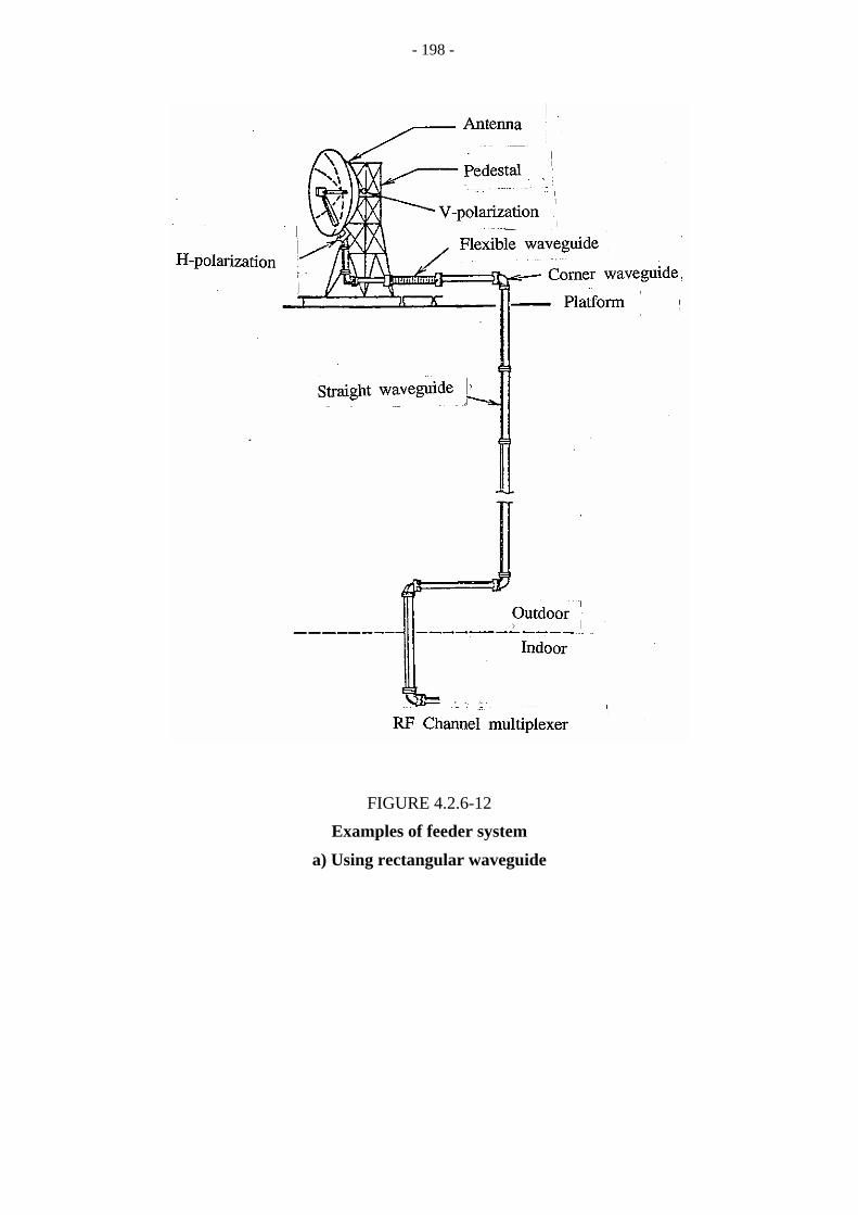
- 198 -

FIGURE 4.2.6-12

Examples of feeder system

a) Using rectangular waveguide

- 199 -

FIGURE 4.2.6-12


b) Using circular waveguide

- 200 -

In the case of b), two polarization components combined at an orthomode transducer (OMT) are transmitted to the other OMT under the tower through over-sized circular waveguide and separated into each polarization component again. In this case, an interference reduction circuit is used to suppress the cross-polarization components caused by the reflector and the over-sized circular waveguide.

Figure 4.2.6-12c) shows a sophisticated feeder system using over-size circular waveguide and handling three different frequency bands (4, 5 and 6 GHz bands). A system multiplexing filter is a key element in this feeder system (see § 4.2.6.6).

FIGURE 4.2.6-12


c) Using over-size frequency bands multiple waveguide handling

- 201 -

Polarizers

A polarizer produces a phase difference between two orthogonally polarized waves. Polarizers with 90° phase difference (90° polarizer) or polarizers with 180° phase difference (180° polarizers) are usually used in antenna feed system: the former for conversion between linearly polarized and circularly polarized waves, and the latter for rotation of the plane of polarization of a linearly polarized wave.

Figure 4.2.6-13 shows a 90° polarizer using a dielectric plate in a circular waveguide operating in the TE11 mode [Kitsuregawa, 1990]. Consider a linearly polarized wave Ei incident with a plane of polarization at an inclination angle of 45° to the dielectric plate. Then, Ei is resolved into two orthogonal components Ei

x and Eiy; Ei

y is parallel to the dielectric plane and Eix perpendicular. Eo

y

(y component of the outgoing wave Eo) is delayed by 90° relative to Eox by passing through the

polarizer, and so the outgoing wave is circularly polarized, but when the phase difference is not equal to 90° or the dielectric plate is lossy, the outgoing wave is elliptically polarized. Figure 4.2.6-14 shows the configuration of a 90° polarizer using a fused quartz plate as the dielectric plate [Kitsuregawa, 1990]. Tapers are provided at both ends of the quartz plate for impedance matching.

FIGURE 4.2.6-13

Conversion from a linearly to a circularly polarized wave by a 90° polarizer using a dielectric plate

- 202 -

FIGURE 4.2.6-14

6 GHz band, 90° polarizer, using a quartz plate

- 203 -

Orthomode transducers

An OMT consists of a common waveguide that transmits two orthogonal dominant modes and two branch waveguides corresponding to these modes; thus, the OMT is a four-port waveguide junction. Figure 4.2.6-15 shows typical examples of OMTs with circular common waveguides. Ports 1 and 2 correspond to the two orthogonal modes, and ports 3 and 4 to the branch waveguides [Kitsuregawa, 1990]. Each branch waveguide couples to each orthogonal mode, respectively; thus, the OMT operates as a polarization coupler. Figures 4.2.6-15a) and b) show OMTs with two longitudinal slots separated by 90° to couple each mode; reflection planes are provided by a short plate in Fig. 4.2.6-15a) and by a tapered waveguide in Fig. 4.2.6-15 b). Figure 4.2.6-15c) shows an OMT with one longitudinal slot and a metallic septum to separate the two modes. The tapered waveguide functions as an open end at the cut-off position. The septum also functions as an open end at the edge for TE11 mode with an electric field parallel to the septum, but does not affect the TE11 mode with a perpendicular electric field.

The position of the longitudinal slots are determined so that the longitudinal magnetic field on the wall of the common waveguide is maximum around the centre of the slots, and the distance d between the centre of the slots and the reflection plane is given as follows. For the short plane:

d ≅ (2n + 1) λg/4

For the tapered waveguide and the septum:

d ≅ nλg/2

where λg is the guide wavelength.

4.2.6.6 System multiplexing filter

The feeder system in Fig. 4.2.6-12c) contains a system multiplexing filter (SMF) which converts 4, 5 and 6 GHz band separate waveguides (six in total) in both polarizations to (or from) a common oversize circular waveguide. This is a particularly important element for wideband antenna and feeder system handling three different frequency bands of 4 GHz (3 600-4 200 MHz), 5 GHz bands (4 400-5 000 MHz) and 6 GHz (5 925-6 425 MHz).

An SMF consists of a 6 GHz band coupler and a 4 and 5 GHz band coupler. The 6 GHz band coupler extracts 6 GHz band signals in both polarizations. A detailed configuration of the 4 and 5 GHz band coupler is shown in Fig. 4.2.6-16. This is the most complicated part of SMF, because the frequency gap between the 4 GHz and 5 GHz bands is as small as 200 MHz.

Radio waves of two polarizations in 4 and 5 GHz bands enter the square waveguide terminal (No. 1 and No. 2). 4 GHz radio waves are reflected at the middle of the waveguide (at the end of the first coupler) and appear at the 4 GHz ports (No. 3 and No. 4), while 5 GHz radio waves pass through the waveguide (first and second coupler) and appear at the 5 GHz ports (No. 5 and No. 6). Operation in the opposite direction is similar. The insertion loss is less than 0.5 dB and cross-polarization coupling is less than -40 dB.

- 204 -

FIGURE 4.2.6-15

Typical examples of orthomode transducers

- 205 -

FIGURE 4.2.6-16

Configuration of 4/5 GHz band coupler in the system multiplexing filter

4.3 Countermeasures

4.3.1 General explanation

4.3.1.1 Purpose of countermeasures

In digital radio-relay systems, circuit performance is often degraded by receiving power reduction or waveform distortion under a multi-path fading environment. System designers should prepare suitable countermeasures so that error performance parameters (e.g. SES probability) could meet the objective.

Basically, countermeasures are intended for the improvement of system performance. ITU-T has recently specified the error performance objectives for end-to-end digital path. In order to achieve radio-relay systems which satisfy these objectives, it is obvious that countermeasures are

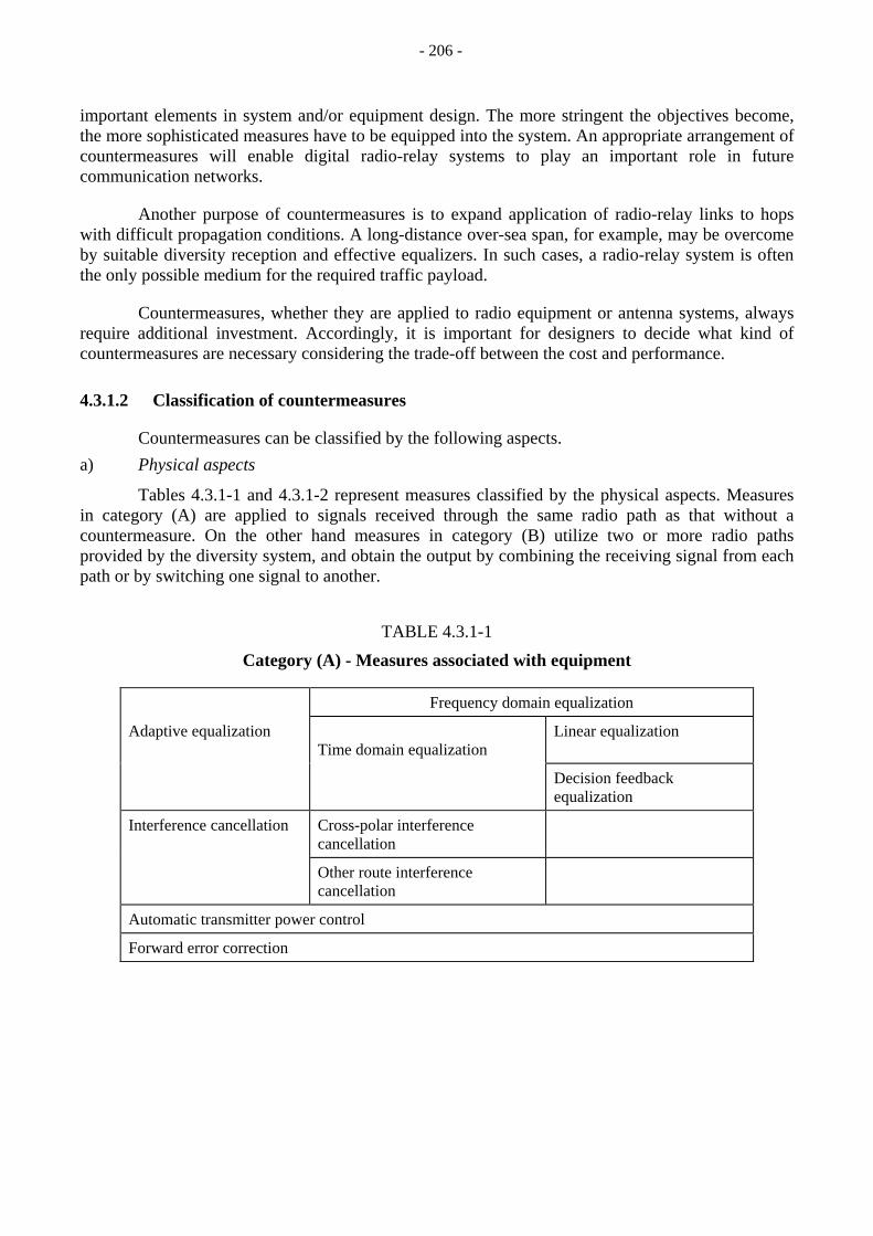
- 206 -

important elements in system and/or equipment design. The more stringent the objectives become, the more sophisticated measures have to be equipped into the system. An appropriate arrangement of countermeasures will enable digital radio-relay systems to play an important role in future communication networks.

Another purpose of countermeasures is to expand application of radio-relay links to hops with difficult propagation conditions. A long-distance over-sea span, for example, may be overcome by suitable diversity reception and effective equalizers. In such cases, a radio-relay system is often the only possible medium for the required traffic payload.

Countermeasures, whether they are applied to radio equipment or antenna systems, always require additional investment. Accordingly, it is important for designers to decide what kind of countermeasures are necessary considering the trade-off between the cost and performance.

4.3.1.2 Classification of countermeasures

Countermeasures can be classified by the following aspects. a) Physical aspects

Tables 4.3.1-1 and 4.3.1-2 represent measures classified by the physical aspects. Measures in category (A) are applied to signals received through the same radio path as that without a countermeasure. On the other hand measures in category (B) utilize two or more radio paths provided by the diversity system, and obtain the output by combining the receiving signal from each path or by switching one signal to another.

TABLE 4.3.1-1

Category (A) - Measures associated with equipment

Frequency domain equalization

Adaptive equalization Time domain equalization

Linear equalization

Decision feedback equalization

Interference cancellation Cross-polar interference cancellation

Other route interference cancellation

Automatic transmitter power control

Forward error correction

- 207 -

TABLE 4.3.1-2

Category (B) - Measures associated with system 3

Space diversity

Dual space diversity

Triple/quadruple space diversity

Angle diversity

Frequency diversity Inband

Crossband

Multi-carrier transmission

b) Functional aspects

Multipath fading brings about power reduction or waveform distortion in the receiving signal, depending on whether the spectrum is reduced totally or partly in the frequency range. The former case, which causes relative increase of thermal and interference noise, can also be observed in analogue systems. The latter case is particularly important in wide-band digital radio systems.

Countermeasures described in a) are designed to compensate for either or both of the above cases.

Table 4.3.1-3 summarizes the classification of countermeasures by the functional aspects.

TABLE 4.3.1-3

Typical countermeasures

Categories Effects

(A) Adaptive equalization Waveform distortion

Interference cancellation Waveform distortion

Measures associated with equipment

Automatic transmitter power control

Power reduction

Forward error correction Power reduction

(B) Space diversity Power reduction and waveform distortion

Measures associated with system

Angle diversity Power reduction and waveform distortion

Frequency diversity Power reduction and waveform distortion

Multi-carrier transmission Waveform distortion

- 208 -

4.3.1.3 Evaluation of countermeasures

An improvement factor of these countermeasures can be defined by the ratio I = P/P ' where P and P ' are system outage probabilities without and with the countermeasures at a given fade depth, respectively. Therefore, the relationship between the degree of the degradation and the corresponding probability has to be clarified. Usually a value “I” depends on the degree of the degradation. In case of space diversity, as shown in Fig. 4.3.1-1, systems with a large fade margin can obtain a larger improvement factor.

Received power reduction (dB)

FIGURE 4.3.1-1

Improvement factor in space diversity

The improvement effects achieved with two different types of countermeasures may not be simply expressed by the simple product of the two improvement factors. For example, in the case of space diversity in combination with adaptive equalizers, there is a synergistic effect, and a larger improvement than the product of the two factors can be expected (see § 4.3.10).

4.3.2 Adaptive equalization


To compensate for signal distortions caused by multipath fading and reduce outage time, the use of adaptive equalizers has become commonplace in digital radio systems. According to the operating frequency, channel equalization can be classified into two types: bandpass equalization and baseband equalization. Usually, the former technique takes place at the intermediate frequency (IF) stage of the receiver and operates in the frequency domain to control the transfer function of the channel.

- 209 -

The simplest frequency-domain equalizer, often referred to as a slope equalizer, only compensates for slope asymmetries which appear in the radio channel response in the presence of multipath fading. It has the function of introducing an amplitude tilt correction which restores symmetry to the power spectral density of the received signal. This can be achieved by monitoring the output power spectrum at two or three frequencies, using a set of narrow-band filters, and comparing the measured powers with each other or with pre-determined undistorted levels. Note that since information on group-delay distortion is generally not obtained in spectrum monitoring process, slope equalizers are usually designed with flat group-delay characteristics. They are primarily able to compensate for frequency-selective fades where any attenuation notch lies outside the passband. Consequently, the main effect of slope equalizers on system signatures is to reduce their frequency width.

Another class of frequency-domain equalizers attempts to produce transfer function that approximates the inverse of channel characteristic conforming to a two-ray propagation model. It consists of a resonator filter whose sharpness factor and centre frequency are controlled to track the fade notch; hence the generic name, notch equalizer. Such circuits always exhibit a concave group-delay characteristic. As a consequence, they tend to produce significant reductions in signal distortion when the channel experiences minimum-phase fading, but double the group-delay distortions for non-minimum phase fading. System signatures for minimum-phase fades can be considerably reduced, while those for non-minimum-phase fades are not improved.

In the following, focus is placed on baseband equalization which operates directly in the time domain and reduces inter-symbol interference (ISI) caused by both amplitude and group-delay distortions. Its basic principle can best be visualized by writing the discrete input/output relationship describing the overall channel response:

(4.3.2-1) where:

xk (τ) = x(kT + τ) is the received complex signal at the sampling instant

ak: data symbol transmitted at time kT

nk: additive white Gaussian noise sample

hi(τ), i = –∝,…,+∝, are the samples of the overall channel impulse response corresponding to the sampling phase τ.

Equation (4.3.2-1) clearly shows that each transmitted symbol is corrupted not only by additive noise, but also by interference from past and future symbols. ISI-free transmission is possible only if the impulse response h(τ) satisfies the Nyquist criterion, i.e., h0(τ) = 1

and

hi(τ) = 0 for i ≠ 0, for some . In practice, the transmit and receive filters are designed to form a Nyquist filter, but the time-variant multipath propagation characterizing the radio channels destroys this property and causes severe ISI. To combat the resulting ISI, an adaptive equalizer is required at the receiver.

4.3.2.2 Equalization structures

There are two basic baseband equalizer structures [Qureshi, 1983; Sari, 1992] to remove the ISI prior to making decisions: linear equalizers and non-linear decision-feedback equalizers. In this subsection, both types of equalizers are described and their potentials discussed. The adaptation algorithms required to make these devices suitable are described in the next subsection.

- 210 -

A linear equalizer (LE) takes the form of a nonrecursive transversal filter with adjustable complex tap-gains (coefficients). Figure 4.3.2-1 shows a LE with N = 2L + 1 taps whose tap-gains are denoted c–L,c–L+1,…,c0,…,cL–1,cL. The equalizer output is given by:

(4.3.2-2)

with ∆ ≤ T denoting a delay element. This output is next passed to a decision circuit which delivers an estimate âk of the data symbol ak. An essential parameter in equalizer design is the number of taps, N . Increasing N improves the static performance (correction capacity) of the equalizer, but also degrades its dynamic performance (convergence and adaptation noise properties).

FIGURE 4.3.2-1

Nonrecursive linear equalizer structure

The equalizer is said to be synchronous when the unit delay ∆ is equal to the symbol period T , and fractionally-spaced when ∆ is smaller than T , e.g., ∆ = T / 2. For synchronous LE, equation (4.3.2-2) can be rewritten in a simpler form:

(4.3.2-3)

Fractionally-spaced equalizers (FSE) were developed to make the receiver insensitive to the sampling phase τ. Performance of synchronous equalizers is indeed strongly dependent on the sampling phase, because the period of its periodic transfer function is 1/ T, and this does not allow it to independently compensate for channel distortions in and outside of the Nyquist bandwidth (−1/ 2T,1/ 2T). More specifically, the equalizer operates on the received signal spectrum folded to the Nyquist bandwidth whose shape depends on the sampler phase. An FSE overcomes this difficulty, because the period of its periodic transfer function is / ∆ ( = 2 / T for ∆ = T / 2 ), which

- 211 -

makes it possible to independently correct the distortions in the Nyquist bandwidth and those in the excess bandwidth.

A decision feedback equalizer (DFE) is a non-linear device composed of two transversal filters as shown in Fig. 4.3.2-2. The inputs to the feedforward filter with N1 taps are the received signal samples, whereas the inputs of the feedback filter with N2 taps are the previously detected data symbols. Using the notation of Fig. 4.3.2-2 and assuming ∆ = T, the DFE output is given by:

(4.3.2-4)

The key idea in DFEs is that if the previous data symbols are decided correctly, their interference on the current data symbol can be removed by feeding them to the feedback filter. DFEs perform better than LEs on severely amplitude-distorted channels such as radio channels which experience multipath fading. An LE can compensate for a spectral notch only at the expense of a substantial noise enhancement. In contrast, a DFE can, in principle, compensate for a spectral notch without noise enhancement, but DFEs suffer from the well-known error propagation phenomenon. A decision error propagates in the delay line of the feedback filter and causes more errors. Despite this phenomenon, DFEs perform better than LEs and turn out to be the appropriate choice for fading channels. Although DFEs yield superior performance to LEs, the latter are often preferred for practical implementations, due to their implementation simplicity. This is particularly true in high-speed digital microwave radio systems.

4.3.2.3 Adaptation algorithms

The algorithms are described considering LEs, but their extension to DFEs is straightforward. Historically, the oldest algorithm for adaptive equalization is the zero-forcing (ZF) algorithm developed by Lucky [1965] at the end of the 1960s. Referring to Fig. 4.3.2-1 which shows an LE with the input signal denoted xk, the tap-gains denoted cj,( j = –L,…,+L), and the output signal denoted yk , the polarity-type ZF algorithm is:

(4.3.2-5)

where:

α : small positive constant denoted step-size

sgn(.) : mathematical sign function

ek : output error signal at time kT, given by ek = yk – âk.

In this algorithm, the reference tap forces the main sample of the equalized impulse response to 1, and every other tap forces one sample of that response to 0.

The most popular algorithm in adaptive channel equalization is the stochastic gradient algorithm which minimizes the mean-square error (MSE) at the equalizer output. It is also known as the least mean square (LMS) algorithm in the literature. Referring back to Fig. 4.3.2-1, the polarity-type version of this algorithm is given by:

(4.3.2-6)

The LMS algorithm minimizes the combined effect of ISI and additive noise, and hence leads to better performance than the ZF algorithm, especially at low signal-to-noise ratios.

FIG

UR

E 4

.3.2

-2

Dec

isio

n-fe

edba

ck e

qual

izer

- 212 -

- 213 -

Unlike the ZF algorithm, the LMS algorithm is easy to analyze in terms of stability, self-noise, and convergence and tracking properties. As the step-size parameter α is increased, convergence of the algorithm becomes faster, but this also increases the algorithm self-noise, i.e., the fluctuation of the tap-gains in the steady-state. The critical step size (the step-size beyond which the algorithm is unstable) is given by:

(4.3.2-7)

where λmax is the largest eigenvalue of the N × N -dimensional autocorrelation matrix R of the

equalizer input signal, and is the signal power at the equalizer input. The optimum value of the step-size parameter is easily shown to be half of the critical value.

The convergence speed of the LMS algorithm is governed by the maximum to the minimum eigenvalue ratio λmax / λmin of the signal autocorrelation matrix R [Proakis, 1989]. The larger this ratio, the slower the convergence speed of the algorithm. On the other hand, λmax / λmin is directly related to the channel amplitude distortion. Consequently, convergence of the LMS algorithm is slow on radio channels with deep spectral nulls.

To minimize outage in digital radio links, it is essential that the equalizer adaptation algorithm does not diverge and keeps tracking the channel variations even if carrier synchronism is lost during deep fades. Otherwise, the equalizer taps require reinitialization after the fade event, and recovery takes a significantly longer time. For this reason, there has been a significant interest by system designers to use blind (or self-recovering) algorithms that are robust to ISI and also to the loss of carrier phase reference.

The first blind algorithm was reported by Sato [1975] for pulse-amplitude modulation (PAM) signals, and blind algorithms for 2-dimensional signals such as PSK and QAM were later developed by Godard [1980] and Benveniste and Goursat [1984]. To our knowledge, none of these approaches to blind equalization has found wide application in digital radio systems, and the simpler maximum level error (MLE) adaptation [Yatsuboshi et al., 1974] remains the preferred choice. This consists of enabling the adaptation algorithm when the sign of the error signal is correct with probability 1 and stopping it otherwise. When the MLE adaptation strategy is applied to the polarity-type LMS algorithm, it reads:

(4.3.2-8)

with:

where W is a predetermined set of windows of the signal constellation plane. For a M 2-state QAM

constellation in which the in-phase and quadrature components take their values from the alphabet ±1,±3,…,±(M – 1), W is defined by |Re(yk)| > M – 1 and |Im(yk)| > M – 1, where Re(.) and Im(.) denote real part and imaginary part respectively.

- 214 -

FSE adaptation has an inherent instability which is due to the fact that the period of the periodic transfer function is usually larger than the received signal bandwidth. In the absence of noise, the equalizer coefficients are not uniquely determined, because the equalizer can synthesize an infinity of different transfer functions in the frequency intervals with vanishing signal spectrum without affecting the output MSE. The equalizer transfer function is unbounded in these regions, and a consequence of this is that the tap-gains may diverge after a long period of stable operation.

To stabilize the FSE operation Gitlin et al. [1981] developed the tap-leakage algorithm which minimizes the cost function:

(4.3.2-9)

where the first term is the conventional MSE, and the second term is proportional to the squared modulus of the equalizer taps. It is given by:

(4.3.2-10)

Stabilization of the FSE operation using the tap-leakage algorithm is naturally achieved at the expense of some increase of the output MSE. It can be shown that this algorithm is equivalent to adding a virtual noise to the signal at the equalizer input. The spectral density of this noise is given by the constant µ in equation (4.3.2-9). This constant must, therefore, be kept small to limit the performance degradation of the FSE.

4.3.3 Interference cancellers


The fading often causes not only a decrease of DRRS desired signal (D) but also an increase of an interference signal (U: undesired signal). One example is a degradation by the interference from another route of the radio-relay system, such as high output power analogue system or wide spread spectrum of DRRS. Another example is a co-channel operation system that uses orthogonal polarization through the same antenna system. The degradation of cross-polarization discrimination (XPD) causes interference between both polarization transmissions.

One of the important degradation factors on path calculation is interference noise from other systems. If interference susceptibility of DRRS becomes better, it facilitates the introduction of same frequency reuse between different systems.

To compensate for the degraded ratio of D/U by fading, an adaptive interference canceller can be applied to DRRS. The basic principle of the interference cancellation is to obtain the source of an interference signal through a certain method, and to control adaptively the phase and amplitude to suppress the interference signal in the desired signal.

Several kinds of interference canceller technology for DRRS have been developed as a countermeasure for fading condition [Murotani and Yamamoto, 1985]. They can be classified into two types: an analogue circuit canceller generally in intermediate frequency (IF) or baseband (BB), and a digital circuit canceller in BB.

With the interference canceller, the performance of DRRS improves rather than without it; it is also effective for efficient spectrum use. A new DRRS can be introduced into an area where severe interference sources exist on the same frequency, if an interference canceller can improve up to

- 215 -

enough D/U on any fading condition. In case of co-channel operation that can transmit the double capacity of DRRS rather than interleaved system, a cross-polarization interference canceller (XPIC) compensates degraded antenna discrimination on multi-path fading condition.

4.3.3.2 Interference cancellers

Other route interference from FM systems with high transmitter power sometimes includes a peak spectrum around the carrier. Figure 4.3.3.-1 shows a block diagram of an example of analogue interference canceller in BB. The analogue interference signal operating at the same channel with DRRS, looks like a line spectrum in the centre of received DRRS signal. It becomes almost a DC component after the detection in the DRRS demodulator, and it degrades the constellation of DRRS signal. The interference DC component can be suppressed by a DC block capacitor. However, the necessary DC component of a digital signal is recovered through the integrator to the input of the decision circuit. At the output of demodulator of DRRS, the interference component is almost cancelled from the received signal. The DRRS equipped with this kind of an interference canceller becomes, under some circumstances, possible to coexist with analogue systems operating on the same frequency channel.

FIGURE 4.3.3-1

Analogue interference canceller

Another method uses a supplementary antenna to receive the interference component as shown in a block diagram in Fig. 4.3.3-2. An analogue interference signal received by a supplementary antenna is controlled the phase and level so as to suppress the interference signal in the desired signal. The control signals are fed from two multipliers, after multiplication of residual interference components (RI and RQ) by a coherent detected interference signal. The cancellation is done in IF or RF, and control signals are processed in BB.

This method does not depend on an interference source, and therefore, it can be applied to any kinds of interference sources. This type of canceller has been realized and applied into 256-QAM system. Then, the D/U was improved by more than 13 dB.

- 216 -

FIGURE 4.3.3-2

Other route interference canceller

4.3.3.3 Cross-polarization interference cancellers

The system operating at the same frequency channel on orthogonal polarization in the same route (co-channel system) can transmit double capacity signal rather than that of the interleaved use. It is possible to achieve high spectral efficiency or to introduce high capacity DRRS in the one route.

Under normal propagation conditions, the improved XPD characteristics of an antenna about the boresight may in some circumstances provide co-channel frequency reuse operation.

However the co-channel systems are seriously affected by co-frequency cross-polarized interference arising from low XPD values that may occur during periods of multi-path fading. The degradations of XPD are caused by propagation phenomena, such as either deep fading into one of the dual polarization signals or severe multi-path reflection signals which include orthogonal

- 217 -

polarization component. In the case of co-channel transmission systems, the required XPD may not be achieved and, therefore, some countermeasures to improve XPD values are required.

Further, propagation conditions vary and depend on many parameters such as path condition, antenna performance, climate, time and so on.

Figure 4.3.3-3 shows a general co-channel transmission model. TV and TH are transmitting signals, Hij are transfer functions of antenna system and space. Kij are transfer functions of equalizers, and XPIC. The channel distortion is compensated at the output signals OV and OH, by an equalizer and the interference signal cancellation by an XPIC, respectively.

FIGURE 4.3.3-3

General co-channel operation model

(4.3.3-1)

(4.3.3-2)

Under the above conditions, there may be a frequency characteristic difference between cross-polar interference signal and its original orthogonal polarization receiving signal. An adaptive canceller shall be applied as a countermeasure against the changing state of cross-polarized interferences at every moment. To cancel the interference signal in the receiving desired signal, it is necessary to make an accurate cancellation signal from another polarization receiving signal.

In digital transmission, a pulse response depends on frequency characteristic of its transmission path. A transversal filter theoretically can generate any shape of a pulse response. An XPIC consisting of transversal filters can compensate the frequency difference between both received polarization signals for an effective cross-polar interference cancellation. XPIC can be implemented in IF or BB stage, but a baseband digitalized processing is easy to introduce LSI technology.

- 218 -

An XPIC with T-space transversal filters compensates nearly at each sampling point (N × T), so it is necessary to adjust different absolute delay time (DADT) correctly between both received signals of orthogonal polarizations.

On the other hand, an XPIC can consist of fractionally tap transversal filters, it has wide tracking range for DADT. It can cover ± N × T/2 in case of a T/2 fractionally tap XPIC, where N is the number of taps of transversal filter and T the 1/symbol rate.

The transversal type XPIC generally employs the correlation algorithm to reduce interference signal as a transversal equalizer reducing inter-symbol interference. The adaptive control algorithm for transversal type XPIC also applies the LMS as described in adaptive equalizers. The LMS algorithm can reduce both noise and interference signal, and converge fast and stable.

Figure 4.3.3-4 shows an example of XPIC cancellation result in 256-QAM system (see Report ITU-R F.378-6, 1990). The digital type of XPIC improves D/U by more than 20 dB.

FIGURE 4.3.3-4

Performance of a cross-polarization interference canceller (XPIC) – One laboratory example

D/U: desired-to-undesired signal ratio C/N: carrier-to-noise ratio

- 219 -

4.3.4 Adaptive transmitter power control


Adaptive transmitter power control (ATPC) is a practice allowing to achieve a number of advantages in radio-relay systems.

As opposed to a fixed operating condition, the microwave transmitter is operated with variable output power in a range from a maximum value Pmax to a minimum (or nominal) value Pnom,at which the transmitter stays for a high percentage of time. Pmax is reached only during unfavourable fading conditions as detected by the far-end receiver, experiencing low receive signal levels.

A backward communication service channel is used to control the transmitter in a feedback loop arrangement.

A possible implementation of an ATPC control loop is shown in Fig. 4.3.4-1.

FIGURE 4.3.4-1

ATPC control loop block diagram

- 220 -

The error signal is derived from the AGC voltage in the receiver IF section and compared with a suitable fixed voltage reference, related to the ATPC threshold (M).

On the transmit side, the processed error signal controls the output power level of the FET amplifier.

The error signal is processed entirely in digital form to take advantage of VLSI integration.

Backward transmission is performed using one of the media dependent bytes of the regenerator section overhead (RSOH) foreseen by ITU-T (see Recommendation ITU-R F.750).

The digital accumulator length determines the main loop time constant and is therefore critical with respect to the maximum fading speed that the loop can control.

4.3.4.2 Applications

The main benefits deriving from the use of an ATPC concept can be listed as follows:

a) Increase of the available system gain in the medium-high BER region (10-6 ≤ BER ≤ 10-3) due to reduction of output back-off (OBO) only under strong fading condition, so that the influence of transmitter lack of linearity is negligible on the BER performance, already impaired by noise or in-band distortion; this leads to a benefit in SES% performances.

b) Sensible reduction in power consumption of the high power amplifier, by possible joint adaptive D.C. feeding of the final stages, with great benefit in MTBF of the FET power devices.

c) Elimination of upfade problems in the receivers.

d) Improvement on outage performance due to reduced influence of adjacent-channel interference (ACI).

e) Easier frequency co-ordination in crowded nodal station due to the reduced nominal received level.

Items a) to d) especially are of fundamental importance for the new generation of SDH radio systems.

In fact the increase of modulation complexity, necessary to cope with the higher rate of the SDH format keeping the radio frequency arrangements unchanged, clearly turns out to be less penalising from a general point of view if the introduction of an ATPC mechanism brings significant improvements both in medium and in the high BER region.

As far as point e) is concerned, the following table reports typical reductions of the minimum angular spacing for frequency reuse or co-polar adjacent frequency operation, between two incoming hops on the same node.

From Table 4.3.4-1 it can be seen that improvements, against “No ATPC” case, in the range of 30% to 70% can be obtained by adopting an ATPC range (R) of 15 dB.

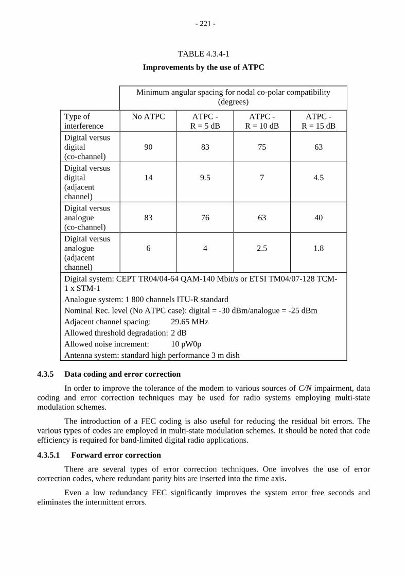
- 221 -

TABLE 4.3.4-1

Improvements by the use of ATPC

Minimum angular spacing for nodal co-polar compatibility (degrees)

Type of interference

No ATPC ATPC - R = 5 dB

ATPC - R = 10 dB

ATPC - R = 15 dB

Digital versus digital (co-channel)

90

83

75

63

Digital versus digital (adjacent channel)

14

9.5

7

4.5

Digital versus analogue (co-channel)

83

76

63

40

Digital versus analogue (adjacent channel)

6

4

2.5

1.8

Digital system: CEPT TR04/04-64 QAM-140 Mbit/s or ETSI TM04/07-128 TCM-1 x STM-1 Analogue system: 1 800 channels ITU-R standard Nominal Rec. level (No ATPC case): digital = -30 dBm/analogue = -25 dBm Adjacent channel spacing: 29.65 MHz Allowed threshold degradation: 2 dB Allowed noise increment: 10 pW0p Antenna system: standard high performance 3 m dish

4.3.5 Data coding and error correction

In order to improve the tolerance of the modem to various sources of C/N impairment, data coding and error correction techniques may be used for radio systems employing multi-state modulation schemes.

The introduction of a FEC coding is also useful for reducing the residual bit errors. The various types of codes are employed in multi-state modulation schemes. It should be noted that code efficiency is required for band-limited digital radio applications.

4.3.5.1 Forward error correction

There are several types of error correction techniques. One involves the use of error correction codes, where redundant parity bits are inserted into the time axis.

Even a low redundancy FEC significantly improves the system error free seconds and eliminates the intermittent errors.

- 222 -

As a matter of fact, FEC coding can be considered as an all-digital alternative to sophisticated RF linearizers, since the big improvement provided at lower BERs is perfectly matched to counteract non-linear distortion effects.

As a consequence, an optimum performance/economy trade-off can be obtained combining the use of moderate IF predistortions and FEC coding.

Two main classes of FEC have been developed: – Block codes

The data sequence is divided into blocks of k symbols and a redundancy of n - k symbols, calculated according to each particular code, is added to the bit stream. In this way it is possible to recover the original transmitted block even in case of dribble errors not exceeding the correction capability of the code. Statistically there is a net coding gain, depending on the added redundancy and the particular algebraic structure of the code.

– Convolutional code In this case the redundancy is added continuously following the coding philosophy; coding

symbols replace the blocks and the distance between the code sequences can be maximized.

4.3.5.2 Coded modulation

This method is a technique that combines coding and modulation which would have been done independently in the conventional method. Redundant bits are inserted in multi-state numbers of transmitted signal constellations. This is known as coded modulation.

Representative examples of coded modulation are block coded modulation (BCM), trellis coded modulation (TCM) and multi-level coded modulation (MLC or MLCM). In BCM, plural levels are coded by block codes whereas TCM uses only convolutional codes. On the other hand, different codes can be used for each coded level in MLCM, so that can be seen as a general concept that includes BCM and to some extent TCM. These schemes require added receiver complexity in the form of a maximum likelihood decoder with soft decision.

A technique similar to TCM is the partial response, sometimes called duo-binary or correlative signalling system. A controlled amount of inter-symbol interference, or redundancy, is introduced into the channel. Hence, the signal constellation is expanded without increasing the transmitted data bandwidth. There are various methods utilizing this redundancy to detect and then correct errors to improve performance. This process is called ambiguity zone detection (AZD).

These various methods are briefly described below.

Block coded modulation

BCM is a technique for generating multidimensional signal constellations which have both large distances (i.e. good error performance) and also regular structures allowing an efficient parallel demodulation architecture called staged decoding. It is to obtain a subset of the Cartesian product of a number of elementary (i.e. low dimensional) signal sets by itself. The staged construction allows demodulation algorithm based on projection of the signal set into lower-dimensional, lower-size constellations. These algorithms lend themselves quite naturally to a pipelined architecture.

- 223 -

Multi-dimensional signals with large distances can be generated by combining algebraic codes of increasing Hamming distance with nested signal constellations of decreasing Euclidean distance.

Compared to TCM, BCM schemes give smaller coding gains, but – BCM often requires a lower demodulator complexity than a TCM scheme with the same

performance; – BCM lends itself to a parallel demodulator architecture, which might prove a bonus if high

processing speeds are necessary.

The construction of practical BCM schemes can be based on the “step partitioning” of the signal constellation. Table 4.3.5-1 gives the coding gains over the uncoded reference system corresponding to the same number of net information bits per transmitted symbol, in the case of BCM families based on one-step partitioning (or “B-partition”) and on two-step partitioning (or “C-partition”). The results are relevant to additive white Gaussian noise (AWGN) channels.

Detection is based on the choice of the codeword which is nearest to the received sequence in the Euclidean distance sense. A particular case of BCM can improve the coding gain in a range of BER from 10-3 to 10-4 without greatly increasing the number of redundant bits, by introducing block codes into multi-state modulation schemes. In the case of a 256-QAM signal transmission system, the introduction of block codes into only 2 of the 8 bit baseband signal streams can improve error correction performance. This is because this method enables the addition of four times the number of redundant bits than conventional error correction schemes.

The code bits (2 bits) are used as “subset” signals and the remaining uncoded bits (6 bits) are mapped into signal space so as to maximize the Euclidean distance based on the Ungerboeck’s Set-Partitioning method. Subset signals are decoded in a process based on a conventional error correcting algorithm. Error correction of uncoded bits is performed only if the subset signal is corrected. At the specific time-slot, the uncoded bits are decoded by selecting a signal point that is located nearest to the received signal point from the coded subset signals using soft-decision information.

When the BCH (31,11) code is employed as the above-mentioned block code modulation, a coding gain of about 5 dB can be obtained at BER of 10-4 . The application of block code modulation has led to a coding gain of about 5 dB at a BER of 10-4.

TABLE 4.3.5-1

Coding gains (dB) over the corresponding uncoded QAM system

Uncoded signal

constellation

BCM signal

constellation

Kind of

partition

Block-code

length (n)

No. of dimensions

(2n)

Asymptoticcoding gain

(dB)

16-QAM 24-QAM 24-QAM

B B

2 4

4 8

1.5 2.6

64-QAM 96-QAM 80-QAM

B B

2 4

4 8

1.8 2.6

64-QAM 128-QAM C 4 8 3.1 256-QAM 368-QAM

368-QAM B B

2 4

4 8

1.7 2.5

- 224 -

Trellis coded modulation

Trellis coded modulations are explained as generalized convolutional coding with non-binary signals optimized to achieve large “free Euclidean distance” dE among sequences of transmitted symbols. As a result, a lower signal-to-noise ratio or a smaller bandwidth is required to transmit data at a given rate and error probability.

To achieve this, a redundant signal alphabet is used. It is obtained by convolutionally encoding k out of n information bits to be transmitted at a certain time. The convolutional code has rate k/(k + 1), and adds 1 bit redundancy. In the symbol-mapping procedure that follows the convolutional encoder, the encoder bits determine the subset (or “sub-modulation”) to which the transmitted symbol belongs, and the uncoded bits determine a particular signal point in that subset. The mapping procedure is also called “set-partitioning” and has the purpose of increasing the minimum distance dE among the symbols.

The optimum receiver for the trellis coded sequence requires a maximum likelihood sequence estimation (MLSE) that can be implemented as a Viterbi algorithm.

Since the redundancy of coding in the time domain, as used in serial FEC, is replaced by a “spatial” redundancy, the cost of coding gain is not an increase of the necessary transmission bandwidth, but a higher modulation complexity.

Another advantage of TCMs is their higher flexibility with respect to serial coding, because of the possibility of increasing the constellation efficiency by 1 bit/symbol (in the case of 4-D codes). On an additive white Gaussian noise channel, the coding gain over an uncoded reference system is represented in Fig. 4.3.5-1.

The coding gain over the uncoded reference system (corresponding to the same number of net information bits per transmitted symbol) is about 2 dB at BER = 10-3 and about 4 dB at BER = 10-10, in the case of 2-D codes. In the case of 4-D codes, such gains are 1.8 dB and 3.5 dB respectively. Some practical values have also been reported (see Fig. 4.3.5-1).

Studies have shown that, when used in conjunction with an adaptive equalizer of medium complexity, uncoded and TCM systems offer nearly the same performance over multipath fading channels. However, the improvement for lower BER values increases as the BER decreases.

Moreover, it has also been shown that the coding gain of a TCM system on a non-linear channel is greater that on a linear one. This advantage of TCMs is of crucial importance to reduce residual BER in case of high complexity modulation schemes.

An application of TCM has been proposed with the aim of not increasing the number of signal symbols, at the cost of a bandwidth expansion of about 14%. In this case, 8 bit baseband signal streams for uncoded 256-QAM are transformed into 7 bit baseband signal streams by a speed converter and then transmitted as 256-TCM.

- 225 -

FIGURE 4.3.5-1

Expected trellis coded modulation (TCM) performance versus the number of net information bits per symbol,

compared against the corresponding uncoded system

Multi-level coded modulation

In MLCM, each level, in set partitioning, is regarded as an independent transmission path with different minimum square distance, and a different code with different strength is applied to each level. An example of set partitioning of 16-QAM is shown in Fig. 4.3.5-2. In that figure, the total set of 16 states (A) is divided into subsets B0 and B1 which are further divided into subsets C0, C2 and C1, C3 respectively. In the subsets Ci (i = 0 to 3), minimum square distance is 4d

2. The same partition is done until the number of state becomes one in each subset. Hence, 16 states are divided into sets of subsets with increased minimum square distance. However, in this stage, error performance of level 1 is determined by the minimum square distance of (A) states set. Then in order to increase “free Euclidean distance” dE, coding is performed to the lower level. Hence the total error performance is improved. Codes used in MLCM are not restricted to only convolutional code.

- 226 -

However, convolutional code may be used for the lower levels, other codes like block code can be used for other levels. Coding rate for MLCM can be selected rather freely because coding rates of each levels are chosen separately. For example, in the case of 16-QAM, if the coding rate of level 1 is 1/2 and 3/4 for level 2 and 23/24 for level 3 and no coding for level 4, the total coding rate R becomes:

R = ( 1/2 + 3/4 + 23/24 + 1 ) /4 = 3.2/4

The outputs of each encoder are converted from parallel to serial and applied into mapping circuit. Therefore the results of one coding corresponds to plural symbols. Consequently, the coding speed is at least half of modulation speed. The coding gain of MLCM depends on its coding rate and coding methods.

Decoding is done by the method called “multi-stage decoding”. At first, the lowest level is decoded and according to the result, the next level is decoded. Further upper levels are decoded in the same way.

Simplified block diagrams of TCM and MLCM are shown in Fig. 4.3.5-3. Figure 4.3.5-4 shows a calculated comparison between BER performance for 128-QAM systems with different redundancies.

FIGURE 4.3.5-2

16-QAM set partitioning

- 227 -

FIGURE 4.3.5-3

Block diagram of coded modulation (transmitter side)

Partial response with soft decoder

Partial response technology is applied as quadrature partial response (QPR) for a digital radio-relay system. In order to improve BER characteristics, QPR may be combined with other coding technologies. One is ambiguity zone detection (AZD), which is a simple form of maximum likelihood (soft) decoder. A detailed explanation of how AZD works follows. “Eye diagram” and “Block diagram of AZD correction” are shown in Figs. 4.3.5-5 and 4.3.5-6, respectively.

Partial response coding forbids certain sequences of symbols. If M is the number of baseband level from partial response coding, then the coded signal cannot transverse more than N level between consecutive symbols, where N is (M + 1)/2. The only way such forbidden sequences can occur is when a symbol has been received in error. The assumption is errors are caused by white Gaussian noise, and are displaced one level only from the correct level into adjacent levels. This is a valid assumption under normal received S/N of interest. When such a forbidden sequence occurs, it is called a partial response violation (PRV). The probability of detecting PRV given a symbol error that has occurred in past D symbol is:

P = 1 - ( 1 - 1/N)D

- 228 -

FIGURE 4.3.5-4

Calculated BER comparison for 128-QAM systems

- 229 -

In an AZD decoder, the eye is divided vertically between the pinpoints (ideal locations of the eye centres) into two types of regions. The symbols sampled in the regions closest to the pinpoints are given an ambiguity weight of 0. Other regions, or the ambiguity zones, are further from the tiny pinpoints and given an ambiguity weight of 1. Their relative ambiguity positions above or below pinpoints are also marked for later error correction. Symbols measured in the ambiguity zones are far more likely to be in error than symbols closer to the pinpoints and are considered to be suspect. The decoded symbols and their ambiguity weights and position markers are fed into the error (PRV) detection and correction circuitry.

When a PRV is detected, the decoder will look back D symbols to see if any decision is made in the ambiguity zone, that is with an ambiguity weight of 1. A correction is made if, and only if, both conditions are met. The decoder tracks only one PRV at a time and associates the nearest ambiguity decision to the PRV. The correction is made by pushing the ambiguity decision one level up or down using the position marker.

FIGURE 4.3.5-5

9 QPR eye diagram

- 230 -

FIGURE 4.3.5-6

AZD correction

4.3.6 Space diversity


Space diversity is usually implemented using two or more receiving antennas with a vertical separation large enough to provide signals in which the impairments due to multi-path fading are sufficiently decorrelated.

Antenna separation is usually designed to correspond to half of the height-pattern pitch of the receiving power. A height-pattern pitch depends on such propagation path parameters as the hop distance, the equivalent Earth radius and the antenna heights at both stations. Detailed information on suitable antenna separation is described in [Yonezawa,1973].

The configuration of space diversity is shown in Fig. 4.3.6-1. The received radio waves travel through different transmission paths so that they are not likely to be affected simultaneously by fading. Therefore, space diversity is effective for both receiving power reduction and signal distortion.

- 231 -

FIGURE 4.3.6-1

Space diversity configuration

4.3.6.2 Methods of obtaining diversity signals

a) Combining methods

Combining diversity reception systems are classified into three configurations according to the frequency band, i.e. radio frequency, intermediate frequency and baseband frequency. Figure 4.3.6-2 shows a space diversity combiner configuration in each frequency band.

Although radio frequency combiners have the simplest configuration with only one receiver, it requires a phase shifter employing waveguide and mechanical devices. Accordingly, it is not considered to be reliable compared to intermediate frequency combiners with an electric endless phase shifter. Base-band combiners using two receivers and demodulators are less cost-effective and more sophisticated than the other two combiners. Therefore, intermediate frequency combiners composed of electric devices generally have the highest reliability and performance compared to other types of the combiners.

There are three types of signal combining methods. The first type is an internal sensing method whose direction of phase variation is driven by the signals derived from phase-modulated received signals [Karabinis, 1983]. The second type is an external sensing method. A phase modulator of the internal sensing method is inserted in the feeder, while the modulator of the external sensing method is inserted in the branched-line from the feeder. The third type is a navigation method whose direction of phase variation is driven by the signal derived from a phase detector which detects the received signal [Ichikawa et al., 1991].

- 232 -

FIGURE 4.3.6-2

Space diversity configuration classified according to frequency band

The features of the above-mentioned methods are as follows. The first method is simplest in the configuration. This method, however, is likely to have degradation caused by the influence of phase-modulation. The second method has no such degradation but the configuration becomes sophisticated. The third method is only applied for co-phase combiner systems and has a comparatively simple configuration.

b) Switching methods

In switching diversity reception, switching is usually done in intermediate frequency (IF) bands. In IF switching diversity, an output signal is selected from the two receivers by a diode switch. Switching control is done in such a way that the level difference between two receiver outputs exceeds 5 dB.

- 233 -

The principle for detecting the level difference is illustrated in Fig. 4.3.6-3. Parts of the IF pre-amplifier outputs are sent to the keying switch, which is driven by an approximately 10 kHz keying signal, and then are sent alternately to an auxiliary IF amplifier equipped with an AGC circuit. The time constant of the AGC circuit is large in comparison with one period of the keying signal but is minimized to always be responsive to the fluctuation of the received signal level caused by fading. The mean signal level of the auxiliary IF amplifier output is kept constant even when there is a great change in input signal strength.

When the auxiliary IF amplifier output is detected, a square wave output corresponding to the relative difference between the two signal levels can be obtained regardless of the absolute value of the IF input levels. Thereafter, by providing the square wave output to a synchronous detector, the positive or negative DC voltage proportional to the relative difference of levels is obtained and then is processed by a logic circuit to obtain a control signal. This control signal is applied to the diode switch selector to choose the signal having the better S/N.

FIGURE 4.3.6-3

Schematic block diagram of IF switching diversity

- 234 -

4.3.6.3 Signal control methods

Signal control methods in combining diversity include the maximum power combiner, the maximal-ratio combiner and the minimum dispersion combiner.

a) Maximum power combiner

The maximum power (MAP) combiner combines two received signals on a co-phase basis in order to maximize the level of the output signal.

A simplified block diagram of the maximum power combiner providing two signal inputs to a continuous combiner is shown in Fig. 4.3.6-4. For the purpose of generating a phase-control signal, the phase of the signal from the diversity antenna is perturbed, resulting in a periodic modulation of the combined-signal power. The fundamental component of the phase modulation contained in the combined-signal is detected and used for a feedback arrangement to control the phase-shifter. The phase correction is chosen to maximize the average power of the combined-signal [Karabinis, 1983].

FIGURE 4.3.6-4

Block diagram of maximum power combiner

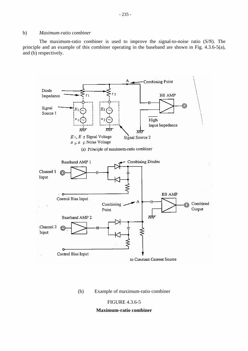
- 235 -

b) Maximum-ratio combiner

The maximum-ratio combiner is used to improve the signal-to-noise ratio (S/N). The principle and an example of this combiner operating in the baseband are shown in Fig. 4.3.6-5(a), and (b) respectively.

(b) Example of maximum-ratio combiner

FIGURE 4.3.6-5

Maximum-ratio combiner

- 236 -

As the two signal voltages E1 and E2 are adjusted to the same value, no current flows through the diodes. Accordingly, the signal level at the combining point A is always equal to the voltage of each signal source regardless of diode impedances, r1 and r2.

Unlike the signal voltages, the noises contained in the two signals have a random level and phase, therefore, their current flows through the diodes. The level of the combined noise at the point A can thus be minimized by changing the diode impedance ratio.

If the diode impedance ratio is so controlled as to satisfy the relation of r2/r1 = (n2/n1)2, the S/N of the combiner can be maintained at maximum at all times [Yonezawa, 1973]. c) Minimum dispersion combiner

The minimum dispersion combiner (MID) can suppress in-band dispersion. An example of the MID combiner configuration is given in Fig. 4.3.6-6. A combined signal spectrum level is monitored at several frequencies by narrow-band filters and detectors. The endless phase shifter is then rotated to an arbitrary direction, and the combined signal spectrum levels are monitored again. From both spectrum levels, two peak-to-peak in-band amplitude dispersions are calculated. After comparing these two in-band amplitude dispersions, the phase shifter is rotated to the direction in which the in-band amplitude dispersion decreases. A microcomputer is used for the control of the above process [Komaki et al., 1984].

FIGURE 4.3.6-6

MID combiner block diagram

- 237 -

In a system using an MID combiner, receiving power attenuation is larger than that employing a MAP combiner when the interfering rays are cancelled out. Therefore, the dual use of a MID combiner and a MAP combiner is necessary to reduce combined-signal level loss. A typical combiner operates as a MID combiner when the combined-signal attenuation is smaller than the pre-designed threshold (usually 10-20 dB) and operates as the MAP combiner when the signal attenuation exceeds the above threshold. d) Specific control method in multi-carrier transmission

For a single-carrier wideband DRRS, the minimum in-band amplitude dispersion space diversity (MID-SD) is generally used. The MID-SD combiner used in multi-carrier systems is an improved notch-detection type (ND-SD) [Ichikawa, 1991]. For multi-carrier systems, an individual in-phase MAP-SD is also effective in multi-path fading condition [Ichikawa et al., 1991].

Figure 4.3.6-7 shows the comparison between the effects of ND-SD and the multi-carrier individual in-phase SD. The latter has about five times a larger improvement factor.

FIGURE 4.3.6-7

Cumulative BER distribution observed in the field test (Daikai - Kishiwada in Japan)

- 238 -

4.3.6.4 Improvement effects

Space diversity on line-of-sight radio-relay systems has two principal functions to improve the transmission quality of radio links. The first is recovering the faded signal and the second is reducing the in-band amplitude dispersion.

1) Improvement on receiving power reduction

In analogue or narrow-band digital radio systems, the effect of the space diversity system is reflected in gaining receiving power level. For these systems, it is sufficient to determine the improvement effect from the statistics of fading at a single frequency. In such a case, a maximum power combiner is usually utilized. This method combines two received signals on a co-phase basis in order to maximize the level of the output signal.

The available improvement from a pair of antennas can be defined as a ratio I0, in which the numerator is the time for which the signal from the main receiving antenna is below the fade margin and the denominator is the time during which the signals from the two receiving antennas are simultaneously below the fade margin. The fraction of a month of high fading activity during which the signal in a radio channel on a space-diversity protected link has a value less than the fade margin is, therefore, P divided by I0, when a perfect switch is used that will always select the stronger of the two received signals.

In terms of variables shown below, the expression for the available improvement on an overland link which has been engineered to have negligible ground reflections is given in Vigants [1975] for values I0 >> 10 by:

(4.3.6-1)

where:

D : path length (km)

f : frequency (GHz)

L : fade margin expressed as a fraction of normal signal voltage

S : vertical separation of receiving antennas (m) centre-to-centre

v : relative voltage (the gain of a secondary antenna relative to the main antenna (dB) is 20 log v)

P : fraction of the month during which the received signal in an unprotected radio channel has a value of less than a particular fade margin, L.

Although the expression for I0 was derived for analogue radio systems, it is widely used for thermal noise considerations in digital radio systems.

- 239 -

Equation (4.3.6-1) has been widely used in the design of DRRS with various parameters. Recent studies on radio propagation within Radiocommunication Study Group 3 adopted the following new equation for improvement factor of space diversity reception (see Recommandation ITU-R P.530):

I0 = [1 − exp F(S,f,D,P0)] x 10 (A − V)/10 (4.3.6-2a)

where:

F(S,f,D,P0) = -3.34 x 10-4 S 0.87 f - 0.12 D 0.48 P0 -1.04

P0 = Pw x 10A/10 /100

V = | G1 – G2 |

with:

A : fade depth (dB) for the unprotected path

Pw : percentage of time fade depth A at single frequency exceeded

P0 : fading occurrence factor

S : vertical separation (centre-to-centre) of receiving antennas (m)

f : frequency (GHz)


G1, G2 : gains of the two antennas.

Recommendation ITU-R P.530 indicates that equation (4.3.6-2a) is valid for the following ranges of variables:

43 ≤ d ≤ 240 km, 2 ≤ f ≤ 11 GHz and 3 ≤ S ≤ 23 m

In the case of a Rayleigh fading model, the improvement factor I0 can be calculated more simply. The slope of cumulative distributions of received power under non-diversity reception is 10 dB/decade, while the slope under space diversity reception is theoretically approximated by 5 dB/decade.

The diversity improvement factor I0 for fade depth A (dB) is defined by:

I0 = P(A)/Pd(A)

where:

Pd(A): percentage of time in the diversity signal branch with fade depth larger than A

P(A): percentage for the unprotected path.

The diversity improvement factor for received power A can be calculated using the above relation in the distribution slope as follows:

(4.3.6-2b)

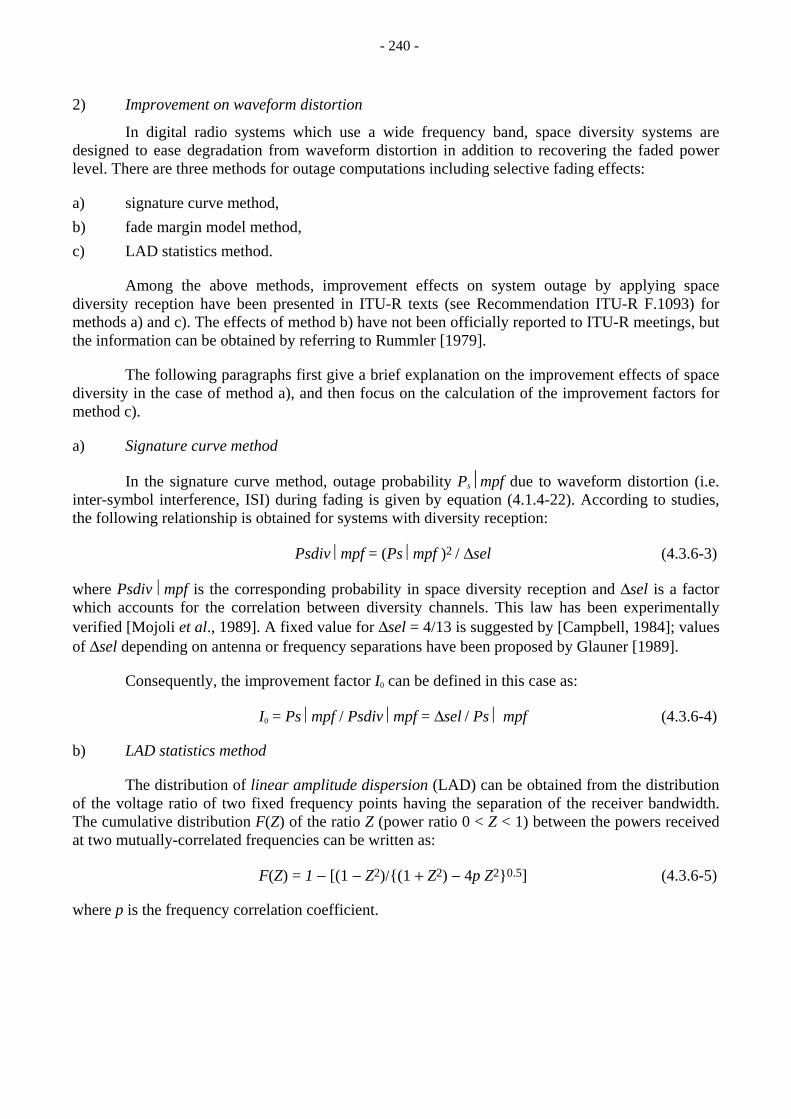
- 240 -

2) Improvement on waveform distortion

In digital radio systems which use a wide frequency band, space diversity systems are designed to ease degradation from waveform distortion in addition to recovering the faded power level. There are three methods for outage computations including selective fading effects:

a) signature curve method, b) fade margin model method, c) LAD statistics method.

Among the above methods, improvement effects on system outage by applying space diversity reception have been presented in ITU-R texts (see Recommendation ITU-R F.1093) for methods a) and c). The effects of method b) have not been officially reported to ITU-R meetings, but the information can be obtained by referring to Rummler [1979].

The following paragraphs first give a brief explanation on the improvement effects of space diversity in the case of method a), and then focus on the calculation of the improvement factors for method c).

a) Signature curve method

In the signature curve method, outage probability Psmpf due to waveform distortion (i.e. inter-symbol interference, ISI) during fading is given by equation (4.1.4-22). According to studies, the following relationship is obtained for systems with diversity reception:

Psdiv ⎢mpf = (Ps ⎢mpf )2 / ∆sel (4.3.6-3)

where Psdiv ⎢mpf is the corresponding probability in space diversity reception and ∆sel is a factor which accounts for the correlation between diversity channels. This law has been experimentally verified [Mojoli et al., 1989]. A fixed value for ∆sel = 4/13 is suggested by [Campbell, 1984]; values of ∆sel depending on antenna or frequency separations have been proposed by Glauner [1989].

Consequently, the improvement factor I0 can be defined in this case as:

I0 = Ps ⎢mpf / Psdiv ⎢mpf = ∆sel / Ps ⎢ mpf (4.3.6-4)

b) LAD statistics method

The distribution of linear amplitude dispersion (LAD) can be obtained from the distribution of the voltage ratio of two fixed frequency points having the separation of the receiver bandwidth. The cumulative distribution F(Z) of the ratio Z (power ratio 0 < Z < 1) between the powers received at two mutually-correlated frequencies can be written as:

F(Z) = 1 − [(1 − Z2)/(1 + Z2) − 4p Z20.5] (4.3.6-5)

where p is the frequency correlation coefficient.

- 241 -

In case of space diversity reception, the cumulative distribution FSD(Z) is expressed by F(Z) as:

FSD(Z) = (3/2)F(Z)2 − (1/2)F(Z)3 (4.3.6.6)

The improvement factor I0 is given by the ratio of F(Z) to FSD(Z).

I0 = F(Z)/FSD(Z) = 1/1.5F(Z) − 0.5F(Z)2

In equation (4.3.6-5) F(Z) depends on the parameter ρ which is a function of the frequency separation ∆f. The parameter ρ can be calculated from several propagation parameters, such as reflected wave strength and path difference between the direct and reflected waves.

The detailed calculation method is described in [Sakagami et al., 1982]. Calculated examples of ρ in typical radio paths are given in Table 4.3.6-1. Basic parameters which affect the value of ρ are the power ratio of the direct-to-reflected wave (D/Ur) and the delay time between the two waves (τ).

TABLE 4.3.6-1

Examples of frequency correlation coefficient, ρ (∆f)

Propagation path

Frequency correlation coefficient

D/Ur

(dB)(1) τ

(ns)(2) Hop

length (km)

Antenna height

(m)

Mountain 0.99985 40 10 50 400

Plain 0.99901 20 5 25 200

Sea 0.97864 6 5 50 100

(1) D/Ur (dB) : power ratio of direct-to-reflected wave. (2) τ (ns) : delay time between the two waves.

Variations of ρ in other conditions are illustrated in Figs. 4.3.6-8a) and b). Using equations (4.3.6-5) and (4.3.6-6), F(Z) and FSD(Z) are easily obtained (see Figs. 4.3.6-9a) and b), respectively). The improvement factors I0 calculated from Fig. 4.3.6-9 are shown in Fig. 4.3.6-10.

- 242 -

a) 50 km plain path

b) 50 km sea path

FIGURE 4.3.6-8 Frequency correlation coefficient

- 243 -

a) Single antenna reception : F(Z)

b) SD antenna reception : FSD(Z)

FIGURE 4.3.6-9

Cumulative distribution of linear in-band amplitude dispersion

- 244 -

Improvement factor I0

FIGURE 4.3.6-10

Improvement factor of space diversity reception for waveform distortion

In the system design it is necessary to clarify threshold values of LAD corresponding to system outage. Figure 4.3.6-11 shows the LAD probability for a 200 Mbit/s 16-QAM system with two different types of combiners and without diversity reception. In this figure, it is clear that the probability of BER = 10-3 corresponds to the probability of LAD = 5.5 dB in all cases. Typical values of LAD threshold for other modulation schemes are presented in Table 4.3.6-2. These LAD limits are measured at the condition where the carrier-to-thermal noise ratio is sufficiently large.

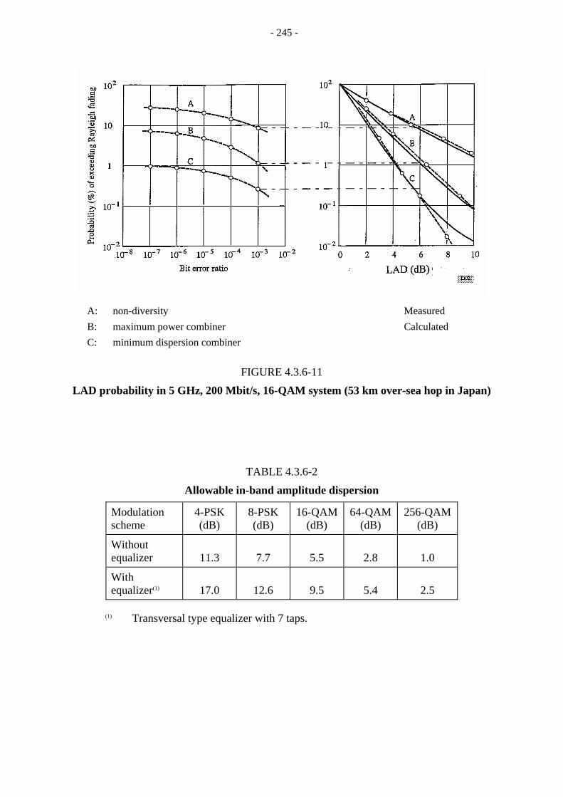
- 245 -

A: non-diversity Measured B: maximum power combiner Calculated C: minimum dispersion combiner

FIGURE 4.3.6-11

LAD probability in 5 GHz, 200 Mbit/s, 16-QAM system (53 km over-sea hop in Japan)

TABLE 4.3.6-2

Allowable in-band amplitude dispersion

Modulation scheme

4-PSK (dB)

8-PSK (dB)

16-QAM(dB)

64-QAM(dB)

256-QAM (dB)

Without equalizer

11.3

7.7

5.5

2.8

1.0

With equalizer(1)

17.0

12.6

9.5

5.4

2.5

(1) Transversal type equalizer with 7 taps.

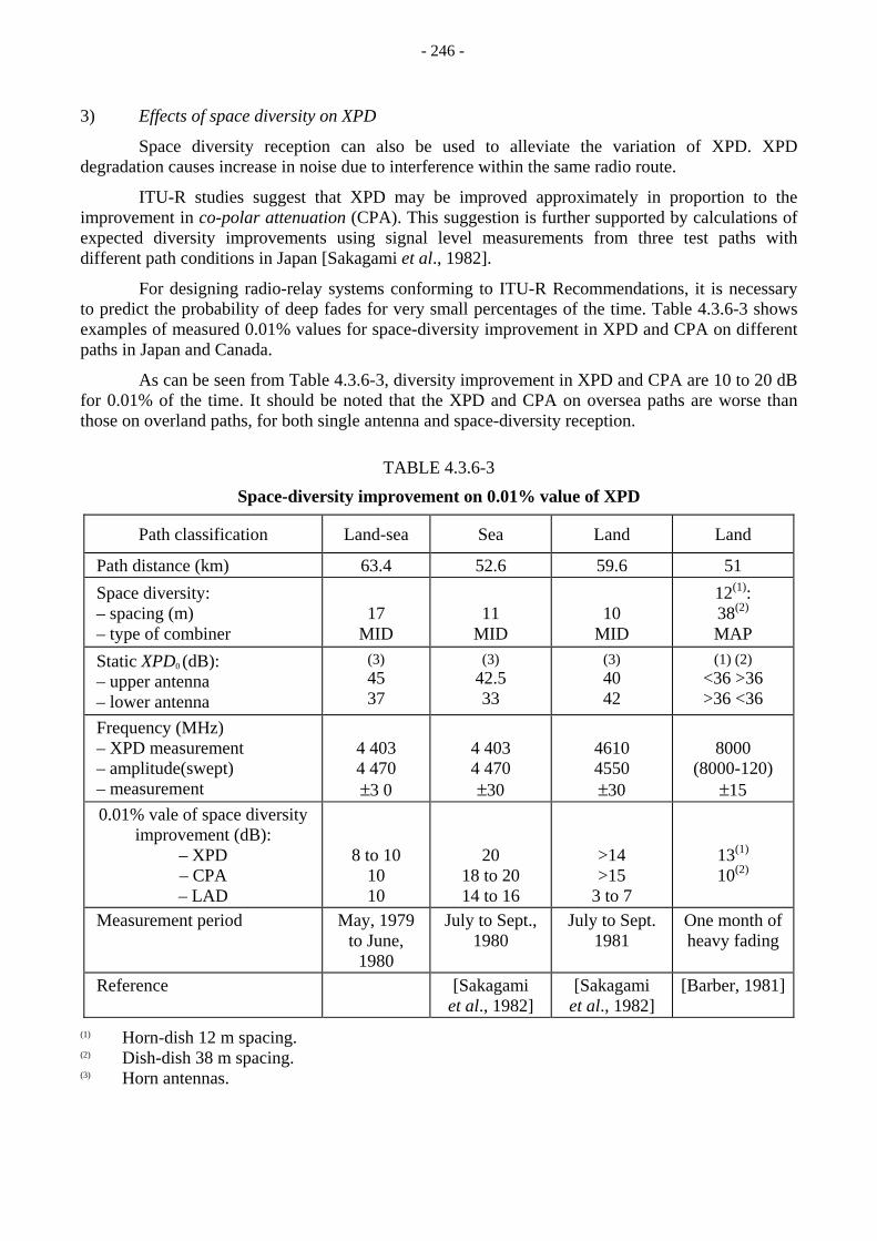
- 246 -

3) Effects of space diversity on XPD

Space diversity reception can also be used to alleviate the variation of XPD. XPD degradation causes increase in noise due to interference within the same radio route.

ITU-R studies suggest that XPD may be improved approximately in proportion to the improvement in co-polar attenuation (CPA). This suggestion is further supported by calculations of expected diversity improvements using signal level measurements from three test paths with different path conditions in Japan [Sakagami et al., 1982].

For designing radio-relay systems conforming to ITU-R Recommendations, it is necessary to predict the probability of deep fades for very small percentages of the time. Table 4.3.6-3 shows examples of measured 0.01% values for space-diversity improvement in XPD and CPA on different paths in Japan and Canada.

As can be seen from Table 4.3.6-3, diversity improvement in XPD and CPA are 10 to 20 dB for 0.01% of the time. It should be noted that the XPD and CPA on oversea paths are worse than those on overland paths, for both single antenna and space-diversity reception.

TABLE 4.3.6-3

Space-diversity improvement on 0.01% value of XPD

Path classification Land-sea Sea Land Land

Path distance (km) 63.4 52.6 59.6 51

Space diversity: – spacing (m) – type of combiner

17

MID

11

MID

10

MID

12(1): 38(2) MAP

Static XPD0 (dB): – upper antenna – lower antenna

(3) 45 37

(3) 42.5 33

(3) 40 42

(1) (2) <36 >36 >36 <36

Frequency (MHz) – XPD measurement – amplitude(swept) – measurement

4 403 4 470 ±3 0

4 403 4 470 ±30

4610 4550 ±30

8000

(8000-120) ±15

0.01% vale of space diversity improvement (dB):

– XPD – CPA – LAD

8 to 10 10 10

20 18 to 20 14 to 16

>14 >15

3 to 7

13(1) 10(2)

Measurement period May, 1979 to June,

1980

July to Sept., 1980

July to Sept. 1981

One month of heavy fading

Reference [Sakagami et al., 1982]

[Sakagami et al., 1982]

[Barber, 1981]

(1) Horn-dish 12 m spacing. (2) Dish-dish 38 m spacing. (3) Horn antennas.

- 247 -

4.3.6.5 Triple and quadruple diversity a) Triple diversity

It sometimes occurs that a space diversity reception with dual antennas does not work well against severe multi-path fadings in extremely anomalous propagation paths. In radio paths such as long-distance over-sea spans, blackout (attenuation type) fading often occurs simultaneously at two receiving antennas with a separation of half of the height-pattern pitch causing the diversity output to be notably degraded. In such cases the third antenna, well-separated from both existing antennas, may provide effective receiving power.

The concept of a triple diversity reception is illustrated in Fig. 4.3.6-12. The output of the dual diversity is combined with the receiving power from the third antenna based on the maximum power algorithm. It is better to obtain a large separation, as far as possible, between the third antenna and the other two antennas so that space correlation in propagation characteristics may become small. Studies on the desirable separation suggests that the following ∆H be recommended:

(4.3.6-7)

where: D : repeater spacing (km) s : path difference between the direct and reflection wave (m) k = [r2/(r2 + 1)]1/2

where r is the reflection coefficient F : frequency (GHz) q : space correlation coefficient (F : 4 GHz → q = 0.5) (F : 6 GHz → q = 0.4)

FIGURE 4.3.6-12

Configuration of triple diversity

- 248 -

In Japan, propagation tests for triple space diversity were carried out on various paths differing in reflection intensity. One of these paths’ profile and antenna arrangement at the receiving station are shown in Fig. 4.3.6-13. This path is classified as a ridge path over water. Figure 4.3.6-14 shows an example of LAD distribution in a 50 MHz band under triple diversity reception measured at the above-mentioned path (Reizan-Itayama link). From the experimental results, the slope of the LAD distribution during fading under triple space diversity reception is 3.3 dB/decade.

FIGURE 4.3.6-13

Example of path profile and receiving antenna allocation for triple diversity

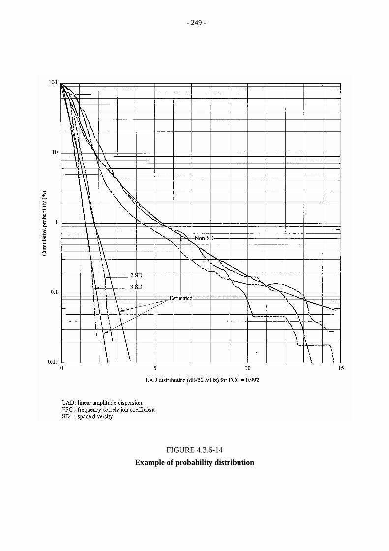
- 249 -

FIGURE 4.3.6-14

Example of probability distribution

- 250 -

b) Quadruple diversity

Field trials of long haul high capacity digital microwave radio systems investigating quadruple diversity were conducted in Australia from 1985 to 1993 [Davey, 1986; 1987; 1989].

The trials, using a combination of dual space and cross band (4 and 6.7 GHz) diversity on long over-water hops, proved that high grade error performance and availability objectives could not be satisfied on these paths with dual space diversity only, and that the addition of cross band diversity achieved useful improvement factors (see Table 4.3.6-4). Operational multi-bearer systems using the quadruple diversity configuration described were successfully established between the mainland of Australia and the island state of Tasmania.

The improvement factors shown in Table 4.3.6-4 were obtained from the error statistics from demodulators simultaneously recording the performance of the different combinations of space and cross frequency band diversity. Refer to Fig. 4.3.6-15.

A field trial of quadruple space diversity was also conducted in Australia in 1983/84 [Davey, 1989]. The IF signals from four vertically spaced antennas were combined, two at a time, with two maximum power combiners. The two signals from the IF combiner were combined in a third IF combiner. The improvement factor of this arrangement was approximately 40 times better than dual space diversity.

Although the quadruple SD trial was a success, and confirmed the predicted large improvement factor, this technique was not adopted for operational systems. Disadvantages of this method are the relatively high cost of the antennas and radio equipment required, and the large tower wind loading associated with the additional antennas.

TABLE 4.3.6-4

Improvement factors – quadruple over dual diversity – worst month (typical month)

Experiment 1 158 km

Experiment 2 116 km

Severely errored seconds

2.6 (15)

6.5 (29)

Degraded min 1.6 (10) 6.2 (30)

Errored seconds 1.4 (7.4) 3.7 (4.5)

Unavailable seconds

2.0 (7.0)

25.0 (>25)

FI

GU

RE

4.3

.6-1

5

Qua

drup

le d

iver

sity

usi

ng d

ual s

pace

and

4 G

Hz

/ 6.7

GH

z cr

oss

band

- 251 -

- 252 -

4.3.7 Angle diversity


Angle diversity is composed of two antenna beams directed in different directions. The second beam is provided either from a separate antenna or from the same antenna with dual-feed dish. The term pattern diversity is often used interchangeably with angle diversity.

Ever since a report indicated that a large improvement could be achieved by angle diversity, many beam tilting propagation tests have been carried out in many countries. Propagation characteristics such as bit error ratio (BER), in-band linear amplitude dispersion (LAD) and cross polarization discrimination (XPD) have been measured in addition to received power. These results have provided various information on improvement effects of angle diversity. For instance, one angle diversity measurement exceeded the improvement effect for a space diversity system, while another did not. These differences suggest that the improvement of angle diversity depends on propagation path conditions and antenna pattern configurations. No theoretical evaluation of the angle diversity effect has been conducted which accounts for the relationship between the angle-of-arrival and the antenna pattern.

Propagation tests to clarify the dependence of path conditions were carried out in certain countries.

4.3.7.2 Applications

In a study on a long (105 km) overwater path, measurements of the power of the received signal, which was an 8-PSK, 45 Mbit/s digital signal at 7.4 GHz, showed significant improvements from angle diversity using a dual-beam antenna [Malaga and Parl, 1985]. In reducing the occurrence of multipath dispersion (LAD) improvement effects were also obtained in an experiment in which two dissimilar antennas with the same boresight angle were mounted side by side [Gardina and Lin, 1985].

The results of two propagation experiments, which were configured to evaluate angle diversity for high capacity digital radio applications, provided further support to the advantages of angle diversity [Lin et al., 1987; Balaban et al.,1987]. The first of these was instrumented at 6 GHz on a 60 km path that was known to provide a strong ground reflection under normal atmospheric conditions. Angle diversity was implemented with a dual-beam antenna, which provided sum and difference voltages as one diversity pair, and a dual beam output as a second pair. In comparison, space diversity was monitored simultaneously with a 3 m conical horn antenna mounted 12.8 m below the main antenna. Diversity signals were obtained by using a maximum power combiner, and fading was monitored by a three-frequency measurement of received power. The distributions of LAD at the output of the combiners (Fig. 4.3.7-1) show that LAD occurred less often with either of the angle diversity input signals than with space diversity inputs during the experiment. In a subsequent period, angle diversity reduced the outage time of a 64-QAM digital radio on this path by factors near 400 [Alley et al.,1987].

- 253 -

FIGURE 4.3.7-1

Distributions showing the effect of angle and space diversity with maximum power combining on the occurrence of in-band power difference (IBPD)

for a 60 km path with ground reflections in the United States of America, at 6 GHz

As part of a series of experiments to determine the effects of small angular and spatial displacements of identical and dissimilar antennas on a 38 km path in Florida [Balaban et al.,1987], angle diversity was implemented in one test with two identical 3 m pyramidal horn antennas mounted side by side. In another experiment in the series, the diversity signal was derived from a smaller (1.8 m) second antenna located just below the main antenna on the tower. The fading was characterized by monitoring the received power at 16 frequencies in a 30 MHz band at 6 GHz. Figure 4.3.7-2 shows the occurrence time statistics of LAD for the two configurations. Although both show substantial reductions in the occurrence time of LAD, the reduction obtained with a vertical separation is significantly greater in this experiment.

- 254 -

FIGURE 4.3.7-2

Distributions showing diversity effects with ideal switching on the occurrence of in-band power difference (IBPD) for a 37 km path near Gainesville, Florida, United States of America, at 6 GHz

Recent propagation experiments comparing angle and space diversity have provided further useful information. In measurements on a 55 km path near Darmstadt, Germany and similarly, on a 51 km path in the east of England, space diversity performed better than angle diversity [Valentin et al., 1987; 1989; Mohamed et al., 1989]. Measurements on a 47.8 km path near Richardson, Texas, United States of America, showed that the advantage of space diversity over angle diversity was dependent on the angle diversity configuration [Allen, 1988; 1989]. A dual-beam antenna with the lower beam crossover aimed at this angle, whereas a configuration using sum and difference signals was better than the dual beam arrangement and almost as good as the space diversity arrangement.

In Japan, similar tests were carried out in several radio paths [Satoh and Sasaki, 1989]. Nagata-Hanase, one of these paths, is an over-water path where a strong sea-reflected wave exists. Since both transmitting and receiving stations are high, the angle separation between the direct and reflected waves is large (0.6-1.1°).

Figure 4.3.7-3 shows the configuration of the antennas. As shown in this figure, two parabolic antennas were installed at the receiving station, having 2.5 m vertical separation, which is not large enough for normal space diversity operation. The beam of the upper antenna was slightly tilted upward.

- 255 -

FIGURE 4.3.7-3

Configuration of receive antennas (Nagata-Hanase, Japan)

Figure 4.3.7-4 shows the improvement effect of space diversity with angle diversity. As shown in this figure, the improvement effect of space diversity with angle diversity is much larger than that of space diversity alone. It is assumed that the large diversity improvement factor on this path is obtained mainly by the beam tilting. This space diversity with angle diversity system is very effective for a path with strong ground-reflection, especially when sufficient vertical separation of two antennas is not ensured.

Comparisons of angle and pattern diversity with space diversity were made by Lin [1988] in experiments in Alabama and Mississippi, United States of America. The results, from one fading season in each location, also showed a performance advantage in a dual-antenna configuration, from aiming one antenna above the nominal angle of arrival, and an advantage of space diversity over angle diversity. The advantage of space diversity in this case was attributed to differences in the fade margins of the radios and to differences in the dispersiveness of the fading on the hops. Based on these, and other, results, the following conclusion was drawn: where digital radio performance is dominated by dispersive effects, angle diversity and space diversity perform equally well; where thermal noise effects predominate, space diversity is a better choice.

- 256 -

FIGURE 4.3.7-4

Received power distribution for space diversity + angle diversity (Nagata-Hanase, Japan)

4.3.8 Polarization diversity

Certain experiments have shown that polarization diversity could be an unexpected but desirable by-product of dual polarized DRRS. In a 1978 investigation [Cronin, 1980] two radios were operated co-channel on V and H polarizations. Even though each channel exhibited the same cumulative fading statistics, there was considerable independence between polarizations in the bit error performance and received signal levels to the channels.

It is however accepted today that the diversity improvement observed by Cronin was a product of the slight differences in the antenna patterns for the two polarizations, effectively providing a pattern or angle diversity effect. Further, by sending the same information on both the V

- 257 -

and H polarizations, use of the orthogonal polarization is effectively denied to another licensee in the area, as if two discrete frequencies (frequency diversity) were used.

True polarization diversity, while effective in systems where propagation is largely by sky wave (such as in the complex multipath fade environment of troposcatter links), has been found to provide little advantage in point-to-point, line-of-sight microwave systems.

4.3.9 Frequency diversity

4.3.9.1 Concept of frequency diversity

One of the most commonly used methods of diversity is frequency diversity, which reduces the effects of multi-path fading. Frequency diversity uses two or more different frequencies to send the same information. The concept of frequency diversity is shown in Fig. 4.3.9-1.

Two advantages can be expected by using frequency diversity. One is to obtain diversity gain and the other is to improve system availability utilizing a redundant path.

As for the frequency separation between the working channel and the protection channel, it is desirable to choose the order of 3 to 5% value of the transmission frequencies.

In actual systems, however, separations around 1 to 2% may give sufficient decorrelation during fading. One experiment reported that dual (1+1) frequency diversity systems with separation of 1 to 5% obtained a 9 to 20 dB diversity gain at 0.01 time percentage level compared to an equivalent non-diversity path [Freeman, 1987].

4.3.9.2 Improvement effect

Theoretical analyses on the improvement effect of frequency diversity have been conducted. One has proposed the following equation for a 1+1 system [Vigants, 1975; Townsend, 1988].

(4.3.9-1)

where:

f : band centre frequecy (GHz)

∆f / f : relative frequency spacing (%)

d : repeater spacing (km)

F : fade depth (dB).

- 258 -

FIGURE 4.3.9-1

Functional block diagram of frequency diversity

In the case that the number of working channels is larger than 1, I decreases from the value calculated by equation (4.3.9-1).

Recent experimental evidence suggests that frequency diversity provides a more effective countermeasure for digital systems than FM systems. In one set of experiments, propagation tests were combined with measurements of the frequency diversity improvement factor for a 16-QAM, 90 Mbit/s digital radio operating in the 6 GHz band on a 42 km path from Atlanta to Palmetto, Georgia, United States of America. By processing the bit error ratio occurrence of the two digital radios, operating in channels with a centre frequency separation of 60 MHz, as the inputs to a 1+1 frequency diversity arrangement with an ideal switch, data from 1980 and 1982 showed frequency diversity improvement factor of 100 and 45 respectively, at a 10-3 bit error ratio. This improvement is comparable to the space diversity improvement factor measured at a 9 m antenna separation with the same radios on this path. In contrast, standard techniques, based on single-frequency fading, predict an improvement factor of 9 for an analogue FM radio with a fade margin between 30 and 35 dB.

- 259 -

An experiment performed at 6 GHz with 90 Mbit/s digital radios in a 1+1 configuration on a 100 km path in Wyoming, United States of America, showed similar frequency diversity improvements for digital radios that exceeded FM predictions by a factor of 10.

However, these results were obtained only at 1+1 configurations. Considering that power spectra of several or more digital systems occupy nearly a whole frequency band, it is likely that more than one radio channel suffers from deep fading at a time. Thus an improvement factor may approximate to, or even become less than, what is predicated for analogue systems.

In an experimental evaluation of a frequency diversity arrangement using a 3+1 multi-line switch, an outage reduction factor of approximately 5 was achieved. The equipment comprised 11 GHz 140 Mbit/s QPSK digital radio which was installed on a single hop. The improvement would be less for the more typical situation of a 5+1 switch protecting a multihop system.

As mentioned above, frequency diversity may be a complementary technique to improve the performance of a digital radio-relay path with a small number of channels.

4.3.10 Synergistic effects

4.3.10.1 Space diversity and adaptive equalizers

As mentioned in § 4.3.1.3, the total effects of two different types of countermeasures usually exceed the simple product of the corresponding individual improvement. This is generally called synergistic effect. Figure 4.3.10-1 illustrates the concept of synergistic effect for space diversity and adaptive equalizers. For the parameters in Fig. 4.3.10-1 it is possible to define the following ξ as the synergistic effect provided that A22 is larger than A12 × A21.

(4.3.10-1)

A value of ξ depends on many factors, such as performances of the applied countermeasures, propagation conditions and so on. It is generally understood that ξ is likely to become larger in systems with small outage probability, i.e. with a large fade margin.

As far as LAD outage is concerned, ξ can be calculated by using equations (4.3.6-2) to (4.3.6-4) and the values in Table 4.3.6-2. A theoretical analysis shows that the synergistic effect is related to the slope of the LAD distribution and as a first approximation is considered to be equal to the equalizer improvement factor A21 [Tajima et al., 1983]. Another approach using signatures also provides the same conclusion [Campbell,1983].

- 260 -

FIGURE 4.3.10-1

Synergistic effect mechanism

Other possible explanations of this synergistic phenomenon are as follows: – A common occurrence during multi-path fading is to observe a flat signal spectrum from the

main antenna simultaneously with the presence of an in-band notch on the diversity antenna, or vice versa. A co-phase combiner processes those signals to give a result having a predominantly linear amplitude slope and significant smaller peak-to-peak amplitude dispersion. Although this distortion can still produce system outage (and hence limit the improvement from diversity alone), it is often almost completely removed by a simple amplitude tilt equalizer [Wang, 1979].

– A statistical analysis of channel characteristics during multi-path fading given in [Anderson et al., 1979] implies that a significant reduction in the proportion of non-minimum phase delay characteristics occurs when diversity signals are processed by a co-phase combiner. Consequently, the use, on the combined signal, of an equalizer designed for minimum phase fades may produce a correspondingly greater improvement in outage factor. This reduction of non-minimum phase delay is even better achieved with an out-of-phase combiner [Komaki et al., 1980].

Experimental studies in several administrations have been reported so far and the results are summarized in Table 4.3.10-1.

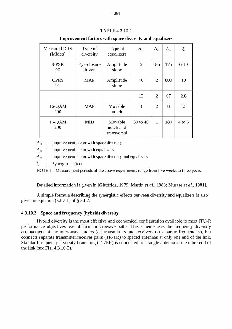
- 261 -

TABLE 4.3.10-1

Improvement factors with space diversity and equalizers

Measured DRS (Mbit/s)

Type of diversity

Type of equalizers

A12 A21 A22 ξ

8-PSK 90

Eye-closure driven

Amplitude slope

6 3-5 175 6-10

QPRS 91

MAP Amplitude slope

40 2 800 10

12 2 67 2.8

16-QAM 200

MAP Movable notch

3 2 8 1.3

16-QAM 200

MID Movable notch and transversal

30 to 40 1 180 4 to 6

A12 : Improvement factor with space diversity A21 : Improvement factor with equalizers A22 : Improvement factor with space diversity and equalizers

ξ : Synergistic effect NOTE 1 – Measurement periods of the above experiments range from five weeks to three years.

Detailed information is given in [Giuffrida, 1979; Martin et al., 1983; Murase et al., 1981].

A simple formula describing the synergistic effects between diversity and equalizers is also given in equation (5.I.7-1) of § 5.I.7.

4.3.10.2 Space and frequency (hybrid) diversity

Hybrid diversity is the most effective and economical configuration available to meet ITU-R performance objectives over difficult microwave paths. This scheme uses the frequency diversity arrangement of the microwave radios (all transmitters and receivers on separate frequencies), but connects separate transmitter/receiver pairs (TR/TR) to spaced antennas at only one end of the link. Standard frequency diversity branching (TT/RR) is connected to a single antenna at the other end of the link (see Fig. 4.3.10-2).

- 262 -

With the highest frequencies (T and R) connected to the top antenna, the link operates standard receive space diversity towards the hybrid diversity site, and transmit space diversity towards the frequency diversity site at the other end. With the upper frequencies transmitting/receiving on the upper dish, an improvement (reduction in outage) over the link is obtained since effective increase in electrical wavelength separation occurs over standard space diversity (same frequency on both antennas).

Probability of worst month outage is computed using standard ITU-R computation procedures. Diversity improvement is computed using only the space diversity improvement factor. An additional improvement is obtained with the frequency diversity assignments, but usually not used to further reduce outage.

The hybrid diversity (separate antennas) end of the link should be at the low end of a high/low path, or at that end nearest any exposed specular reflection (with an exposed point, geometry calculations should be used to optimize the antenna separation for anticorrelated fading). It is also essential that the higher frequencies be assigned the upper antenna so the space diversity improvement factor is enhanced, not partially cancelled, by the frequency diversity assignment.

Hybrid diversity is used all over the world. Costs are greatly reduced: towers at tandem repeaters sites alternate down the system with two and four antennas configurations. Traditional space diversity protection requires four antenna feeder systems at each repeater station.

4.3.11 Multi-carrier transmission

Wideband DRRSs are sensitive to in-band linear amplitude dispersion (LAD). The broader the occupied bandwidth becomes, the more stringent LAD specification the system requires. To cope with this, a high capacity system can be transmitted through some low-bit-rate carriers whose frequency spectra are arranged within the equivalent bandwidth.

The concept of multi-carrier transmission is illustrated in Fig. 4.3.11-1, presenting a 4-carrier system. A multi-carrier system using narrow band transmission can largely ease LAD requirements for frequency selective fading (see Fig. 4.3.11-2).

This fact brings about dramatic improvement on the system outage probability, assuming the calculated results in Fig. 4.3.6-9. It should be noted that system outage occurs not only from LAD but also from thermal noise. Improvement factors in actual cases may saturate with regard to the number of carriers.

Multi-carrier transmission was at first applied to a long-distance over-sea system in Japan [Yoshida et al., 1983] and since then has been utilized in several administrations.

FIG

UR

E 4

.3.1

0-2

Spac

e an

d fr

eque

ncy

(hyb

rid)

div

ersi

ty

- 263 -

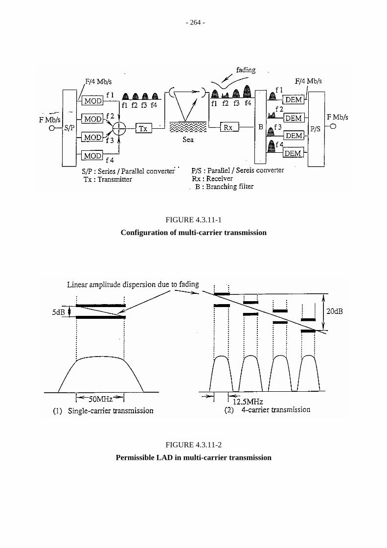
- 264 -

FIGURE 4.3.11-1

Configuration of multi-carrier transmission

FIGURE 4.3.11-2

Permissible LAD in multi-carrier transmission

- 265 -

FIGURE 4.3.11-3

Protection switching in multi-carrier systems

As shown in Fig. 4.3.11-1, the system requires additional modulators, demodulators and other equipment. It depends on the geographical condition of the radio route whether multi-carrier transmission is cost-effective or not. When applying a high capacity DRRS to a route including long-distance hops, multi-carrier transmission may be the best choice. Thus without constructing intermediate stations performance objectives can economically be satisfied.

In general, the use of a multi-carrier method requires the development of linear power amplifiers and the optimization of sub-carrier spacing to avoid intermodulation distortions and intra-system interference produced by adjacent carriers of the same multi-carrier system [D’Aria et al., 1989a].

Examples of the improvement (in terms of signature curves, bit error rate and outage probability) provided by the use of the multi-carrier transmission technique with and without adaptive equalizers are given in [D’Aria et al., 1989b], in the case of 64-QAM radio systems, and in [D’Aria et al., 1989a] in the cases of 256-QAM and TCM radio systems.

Figure 4.3.11-3 shows two methods of protection switching in multi-carrier systems. Method a) is a conventional system switching by a simple control algorithm. For method b), by using a carrier matrix switch more frequency diversity effect can be expected, while it needs a sophisticated control algorithm.

- 266 -


ALLEN, E.W. [1988] Angle diversity test using a single aperture dual-beam antenna. Conf. Record, Vol.3, paper 50.1, 1626-1632. IEEE International Conference on Communications (ICC’88), Philadelphia, PA, United States of America.

ALLEN, E.W. [1989] Angle diversity at 6 GHz: methods of alignment and test results. Conference Record. IEEE International Conference on Communications (ICC’89), Boston, MA, United States of America.

ALLEY, G.D., PENG, W.C., ROBINSON, W.A. and LIN, E.H. [1987] The effect on error performance of angle diversity in a high capacity digital microwave radio system. Conference Record, Vol. 2, Paper 31.4, 1223-1228. Global Telecommunications Conference (Globecom’87), Tokyo, Japan.

ANDERSON, C. W., BARBER, S. G. and PATEL, R. N. [1979] The effect of selective fading on digital radio. IEEE Trans. Comm., Vol. COM-27, 12, 1870-1876.

BACCARINI, L. et al. [1983] Error-Correction Techniques and Adaptive Linialization in SDH Radio. European Conference on Radio-Relay Systems (ECCR’83), 238-243.

BALABAN, P., SWEEDYK, E.A. and AXELING, G.S. [1987] Angle diversity with two antennas; model and experimental results. IEEE International Conference on Communications (ICC’87), Seattle, WA, United States of America.

BARBER, S. [1981] Cofrequency cross-polarized operation of a 91 Mbit/s digital radio. Conference Record, Vol. 3, 46.6.1-46.6.6. IEEE International Conference on Communications (ICC’81), Denver, CO, United States of America.

BEAN, B.R. and DUTTON, E.J. [1966] Radio Meteorology. Dover Publications Inc., New York, NY, United States of America.

BECKMANN, P. and SPIZZICHINO, A. [1963] The Scattering of Electromagnetic Waves from Rough Surfaces. Pergamon Press, Oxford, United Kingdom.

BELLINI, S. et al. [1983] Coding for error correction in high capacity digital radio. European Conference on Radio-Relay Systems (ECRR’83), 166-172.

BENVENISTE, A. and GOURSAT, M. [August, 1984] Blind equalizers. IEEE Trans. Comm., Vol. COM 32, 871-883.

BOITHIAS, L. [1987] Radiowave Propagation. McGraw Hill, New York, United States of America.

CAMPBELL, J. C. [1983] Digital radio outage prediction with space diversity. Electron. Lett. Vol. 19, 23, 1003-1004.

CAMPBELL, J.C. [1984] Outage prediction for the route design of digital radio systems. Australian Telecommunication Research, Vol. 18, 2, 37-49.

CAMPBELL, J.C. and COUTTS, R.P. [1982] Outage prediction of digital radio systems. Electron. Lett. Vol. 18, 25/26, 1071-1072.

- 267 -

CRONIN, P.M. [1980] Dual-polarized digital radio operation in a fading environment. IEEE International Conference on Communications (ICC’80), paper 52.5.

D’ARIA, G., DIONISI, S., PIETROIUSTI, R. and ZINGARELLI, V. [1989a] Advanced transmission techniques for signal and multi-carrier high capacity (2 x 155 Mbit/s) digital radio systems. Conference Record, 209-218. 2nd European Conference on Digital Radio-Relay Systems (ECRR’89), Padua, Italy.

D’ARIA, G., MURATORE, F., PALESTINI V. and ZINGARELLI, V. [1989b] Multi-carrier transmission in 64-QAM microwave digital radio. Conference Record, 52.1.1-52.1.5. IEEE International Conference on Communications (ICC’89), Seattle, WA, United States of America.

DAMOSSO, E. and ORDANO, L. [1989] A prediction model for space frequency and angle diversity improvement evaluation on digital radio links. Proc. 2nd European Conference on Radio-Relay Systems (ECRR’89), Abano Terme, Padua, Italy.

DAVEY, L.J. [1986] Recent High Capacity Digital Radio Field Trials in Australia. Proc. European Conference on Radio-Relay Systems (ECRR’96).

DAVEY, L.J. [September, 1987] High Capacity Digital Radio Field Trials. IREECON’87 Digest, 21.

DAVEY, L.J. [1989] High Capacity Digital Microwave Radio Field Trials. Telecom. Journal of Australia.

DI DONNA, G.D. [1993] A compact BCM modem implementation for SDH access radio. European Conference on Radio-Relay Systems (ECRR’93), 267-272.

EMSHWILLER, M. [June, 1978] Characterization of the performance of PSK digital radio transmission in the presence of multipath fading. Conference Record, Vol. 3, 47.3.1-47.3.6. IEEE International Conference on Communications (ICC’84), Toronto, Canada, 47.3.

FEDI, F. [1981] A simple method for predicting rain attenuation statistics on terrestrial and Earth-space paths. Fondazione Ugo Bardoni, Report 1B1081.

FREEMAN, R.L. [1987] Radio System Design Telecommunications. John Wiley & Sons, Inc.

GARDINA, M.F. and LIN, S.H. [1985] Measured performance of horizontal space diversity on a microwave radio path. Conference Record, Vol. 3, paper 36.6, 1104-1107. IEEE Global Telecommunications Conference (Globecom’85), New Orleans, LA, United States of America.

GIBBINS, C.J. [1986] Improved algorithms for the determination of specific attenuation at sea level by dry air and water vapour, in the frequency range 1-350 GHz. Radio Science, 21, 6, 945-954.

GIGER, A.J. [1991] Low-angle microwave propagation: Physics and Modelling. Artech House, Norwood, MA, United States of America.

GITLIN, R.D., MEADORS, H.C. and WEINSTEIN, S.B. [February, 1981] The tap-leakage algorithm: An algorithm for the stable operation of a digitally implemented, fractionally-spaced adaptive equalizer. Bell Syst. Tech. Journal, Vol. 60, 275-296.

- 268 -

GIUFFRIDA, T.S. [1979] Measurements of the effects of propagation on digital radio systems equipped with space diversity and adaptive equalization. Conf. Record, Vol. 3, 48.1.1-48.1.6. IEEE International Conference on Communications (ICC’79), Boston, MA, United States of America.

GLAUNER, M. [1989] Consideration for the planning of digital radio-relay systems limited by interference and noise. Proc. 2nd European Conference on Radio-Relay Systems (ECRR’89), Abano Terme, Padua, Italy.

GODARD, D. [November, 1980] Self-recovering equalization and carrier tracking in two-dimensional data communications systems. IEEE Trans. Comm., Vol. COM-28, 1867-1875.

HALL, M.P.M. [1979] Effects of the troposphere on radiocommunications. IEE Electromagn. Wave Series, 8. Peter Peregrimus Ltd., London, United Kingdom.

ICHIKAWA, H. et al. [1991] A New Combiner for Multi-antenna Diversity in Multi-carrier Microwave Radio Systems. IEEE International Conference on Communications (ICC’91), 5.4.1-5.4.7.

KARABINIS, P.D. [January, 1983] Maximum-power and amplitude-equalizing algorithms for phase control in space diversity combining. BSTJ, Vol.62, 1, 63-89.

KITSUREGAWA, T. [1990] Advanced Technology in Satellite Communication Antennas: Electrical and Mechanical Design. Artech House Inc., Norwood, MA, United States of America.

KOMAKI, S. et al. [April, 1984] A minimum dispersion combiner for high capacity digital microwave radio. IEEE Trans. Comm., Vol. 32, 4, 419-428.

KOMAKI, S., OKAMOTO, Y. and TAJIMA, K. [1980] Performance of 16-QAM digital radio system using new space diversity. Conf. Record, Vol. 3, 52.2. IEEE International Conference on Communications (ICC’80), Seattle, WA, United States of America.

LIN, S.H. [1988] Measured relative performance of antenna pattern diversity, antenna angle diversity and vertical space diversity in Mississippi. Conference Record, Vol. 3, paper 44.1, 1433-1439. Global Telecommunications Conference (Globecom’88). Hollywood, FL, United States of America.

LIN, E.H., GIGER, A.J. and ALLEY, G.D. [1987] Angle diversity on line-of-sight microwave paths using dual-beam dish antennas. IEEE International Conference on Communications (ICC’87), Seattle, WA, United States of America, paper 23.5.1.

LUCKY, R.W. [April, 1965] Techniques for adaptive equalization of digital communication. BSTJ, Vol. 44, 547-588.

LUNDGREN, C.W. and RUMMLER, W.D. [1979] Digital radio outage due to selective fading: observations versus prediction from laboratory simulations. BSTJ, Vol. 58, 5, 1073-1100.

MAEDA, S. et al. [1993] Advanced SDH radio systems for transport of STM-1. European Conference on Radio-Relay Systems (ECRR’93), 349-354.

MALAGA, A. and PARL, S.A. [1985] Experimental comparison of angle and space diversity for line-of-sight microwave links. Conference Record, Vol. 2, paper 19.2, 382-386. IEEE Military Communications Conference (MILCOM’85), Boston, MA, United States of America.

- 269 -

MARTIN, A. L., CAMPBELL, J. C. and COUTTS. R. P. [1983] Results of a 16-QAM 140 Mbit/s digital radio field experiment. Conference Record, Vol. 3, F 2.2.7-F 2.2.8. IEEE International Conference on Communications (ICC’83), Boston, MA, United States of America.

MOHAMED, S.A., RICHMAN, G.D. and HUISH, P.W. [1989] Results of angle diversity trials by British Telecom. Proc. 2nd European Conference on Radio-Relay Systems (ECRR’89), Abano Terme, Padua, Italy, 321-327.

MOJOLI, L.F., CASIRAGHI, U. and TOMATI, L. [1989] Design method for spectrum efficient digital TV transmission. Proc. 2nd European Conference on Radio-Relay Systems (ECRR’89), Abano Terme, Padua, Italy.

MURASE, T. et al. [1991] Design and Performance of the SDH based microwave digital radio systems. European Conference on Radio-Relay Systems (ECRR’91), 48-55.

MURASE, T., MORITA, K. and KOMAKI, S. [1981] 200 Mbit/s 16-QAM digital radio system with new countermeasure techniques for multipath fading. Conference Record, Vol. 3, 46.1.1-46.1.5. IEEE International Conference on Communications (ICC’81), Denver, CO, United States of America.

MUROTANI, M. and YAMAMOTO, H. [August, 1985] Digital radio transmission (in Japanese). Sangyo Tosho Publishing Co., Tokyo, Japan.

NAKAMURA, K. [1979] A class of error correcting codes for DPSK channels. IEEE International Conference on Communications (ICC’79), 45.4.1-5.

NARDONI, A., BELLANI, R., FILIBERT, G., RICAGNI, A., GIACONI, M. and SEMENZATO, P. [1989] I.F. Signature Measurements. Proc. 2nd European Conference on Radio-Relay Systems (ECRR’89), Abano Terme, Padua, Italy.

OGUCHI, T. [1975] Rain depolarization studies at centimetres and millimetres wavelengths: theory and measurement. J. Radio Res. Labs. (Japan), Vol. 22, 107, 165-211.

OLSEN, R.L. [1981a] Cross-polarization during clear-air conditions on terrestrial links. Radio Science, Vol. 16, 5, 631-647.

OLSEN, R.L. [1981b] Cross-polarization during precipitation on terrestrial links. Radio Science, Vol. 16, 5, 761-779.

OLSEN, R.L. [1981c] A review of theories of coherent radiowave propagation through precipitation media of randomly oriented scatters, and the role of multiple scattering. URSI Open Symposium on Mathematical Model of Radio Propagation, XXth General Assembly of URSI, Washington, DC, United States of America. Radio Science, Vol. 17, 1982.

PROAKIS, J.G. [1989] Digital communications. 2nd Edition, McGraw Hill, New York, United States of America.

PRUPPACHER, H.R. and BEARD, K.V. [1970] A mind tunnel investigation of the internal circulation and shape of water drops falling at terminal velocity in air. Quart. J. Roy. Meteorol. Soc., 96, 247-256.

QURESHI, S.U.H. [March, 1983] Adaptive equalization. IEEE Comm. Magazine, Vol. 20, 2, 1-16.

RUMMLER, W.D. [1979] A new selective fading model: application to fading data. BSTJ, Vol. 58, 1037-1071.

- 270 -

SAKAGAMI, S. and HOSOYA, Y. [1982] Some experimental results on inband amplitude dispersion and a method for estimating inband linear amplitude dispersion. IEEE Trans. Comm., Vol. COM-30, 8.

SAKAGAMI, S., FUKUOKA, H. and HOSOYA, Y. [1982] Multi-path propagation characteristic on digital microwave radio links. Rev. Elec. Comm. Labs., Vol. 30, 5, 907-919.

SARI, H. [July, 1992] Adaptive equalization of digital line-of-sight radio systems. Proc. IFAC International Symposium on Adaptive Systems in Control and Signal Processing, Grenoble, France, 731-736.

SATO, Y. [June, 1975] A method of self-recovering equalization for multilevel amplitude modulation systems. IEEE Trans. Comm., Vol. COM-23, 679-682.

SATOH, A. and SASAKI, O. [1989] Tilted-Beam-, Beam-Width- and Space-Diversity Improvements on Various Paths. IEEE Global Telecomunications Conference (Globecom’89), 2.3.1-2.3.5.

SHAFI, M. [1987] Statistical analysis/simulation of a three ray model for multipath fading with applications to outage prediction. IEEE Journ. on Selected Areas In Comm., 389-402.

TAJIMA, K., KOMAKI, S. and OKAMOTO, Y. [1983] Outage probability of a digital microwave radio equipped with space diversity and adaptive equalizer. Trans. Inst. Electron. Comm. Engrs. (Japan), Vol. J66-B, 5, 583-590.

TOWNSEND, A.A.R. [1988] Digital Line-of-sight Radio Links. Prentice Hall International (United Kingdom) Ltd.

VALENTIN, R., GILOI, H-G. and METZGER, K. [1989] Space versus angle diversity – some results of propagation experiments. Conference Record. IEEE International Conference on Communications (ICC’89), Boston, MA, United States America.

VALENTIN, R., METZGER, K., GILOI, H-G. and DOMBEK, K.-P. [1987] Effects of angle diversity on the performance of line-of-sight digital radio systems. Conference Record, Vol. 2, Paper 31.5, 1229-1232. Global Telecommunications Conference (Globecom'87), Tokyo, Japan.

VIGANTS, A. [January, 1975] Space diversity engineering. BSTJ, Vol. 54, 103-142.

WANG, Y. Y. [1979] Simulation and measured performance of a space diversity combiner for 6 GHz digital radio. IEEE Trans. Comm., Vol. COM-27, 12, 1896.

WATERS, J.W. [1976] Absorption and emission by atmospheric gases. Methods of Experimental Physics, Vol. 12B, Radio Telescopes, 142-176. Ed. M.L. Meeks, Academic Press, New York, United States of America.

WATSON, P.A. et al. [1974] Microphysics of hydrometeors and polarization. Working Group Report III. J. de Recherche Atmos. Vol. 8, 1/2, 477-484.

YAMADA, M., KARASAWA, Y., YASUMAGA, M. and ARBESSER-RASTBURG, B. [1987] An improved prediction method for rain attenuation in satellite communications operating at 10-20 GHz. Radio Science, Vol. 22, 6.

YATSUBOSHI, R., SATA, N. and AOKI, K. [1974] A convergence of automatic equalizers by maximum-level error control. Nat. Conv. Rec., IECE Japan, 2192.

- 271 -

YONEZAWA, S. [1973] Microwave Communication-System Design and New Equipment. Second Edition, Maruzen Company, Ltd. Tokyo, Japan.

YOSHIDA, T., KOMAKI, S. and MORITA, K. [1983] System design and new techniques for an over-water 100 km span digital radio. Conference Record, Vol. 1, Session C2. IEEE International Conference on Communications (ICC’83), Boston, MA, United States of America.

BIBLIOGRAPHY

DAMOSSO, E. [1985] Minimum and non-minimum phase fading effects on digital systems: a new approach to outage prediction, Proc. 4th International Conference on Antennas and Propagation (ICAP 1985), Warwick, United Kingdom.

GREENSTEIN, L.J. and SHAFI, M. [1988] Cancellation of Cross-polarization Interference. Microwave Digital Radio Publication, IEEE Press, 138-140.

RUMMLER, W.D. [1982] A statistical model of multipath fading on a space diversity radio channel. Conference Record, Vol. 2, 3B.4.1-3B.4.6. IEEE International Conference on Communications (ICC’82), Philadelphia, PA, United States of America.

ITU-R Recommendations

Rec. ITU-R F.699 Reference radiation patterns for line-of-sight radio-relay system antennas for use in coordination studies and interference assessment in the frequency range from 1 to about 40 GHz.



Rec. ITU-R F.1101 Characteristics of digital radio-relay systems below about 17 GHz.

Rec. ITU-R P.310 Definitions of terms relating to propagation in non-ionized media.

Rec. ITU-R P.369 Reference atmosphere for refraction.

Rec. ITU-R P.453 The radio refractive index: its formula and refractivity data.

Rec. ITU-R P.525 Calculation of free-space attenuation.

Rec. ITU-R P.526 Propagation by diffraction.

Rec. ITU-R P.527 Electrical characteristics of the surface of the Earth.

- 272 -

Rec. ITU-R P.530 Propagation data and prediction methods required for the design of terrestrial line-of-sight systems.

Rec. ITU-R P.676 Attenuation by atmospheric gases.

Rec. ITU-R P.834 Effects of tropospheric refraction on radiowave propagation.

Rec. ITU-R P.836 Surface water vapour density.

Rec. ITU-R P.837 Characteristics of precipitation for propagation modelling.

Rec. ITU-R P.838 Specific attenuation model for rain for use in prediction methods.

Rec. ITU-R P.840 Attenuation due to clouds and fog.

Rec. ITU-R P.841 Conversion of annual statistics to worst-month statistics.

ITU-R Reports (1990)

Report 378 (Annex to Vol. IX, Part 1) Characteristics of digital radio-relay systems below about 17 GHz.

Report 719 (Annex to Vol. V) Attenuation by atmospheric gases.

Report 721 (Annex to Vol. V) Attenuation by hydrometeors, in particular precipitation, and other atmospheric particles.

Report 722 (Annex to Vol. V) Cross-polarization due to the atmosphere.

Report 784 (Annex to Vol. IX, Part 1) Effects of propagation on the design and operation of line-of-sight radio-relay systems.

Report 882 (Annex to Vol. V) Scattering by precipitation.

Report 1054 (Annex to Vol. IX, Part 1) Interference in radio-relay systems caused by terrain scattering.


ITU-T Rec. G.652 Characteristics of a single-mode optical fibre cable.

ITU-T Rec. G.653 Characteristics of a dispersion-shifted single-mode optical fibre cable.

ITU-T Rec. G.654 Characteristics of a 1550 nm wavelength loss-minimized single-mode optical fibre cable.


ITU-T Rec. G.957 Optical interfaces for equipments and systems relating to the synchronous digital hierarchy.

- 273 -

CHAPTER 5

LINK ENGINEERING

5.1 General network and link design considerations

5.1.1 Performance objectives and network planning aspects

The purpose of link engineering is to produce a design of radio routes and individual radio hops, with performances in the field that are likely to comply with a set of performance objectives. Normally, planning objectives derived from ITU’s Recommendations for international connections are applied. Besides complying with such objectives, the design should also result in an optimum of both costs and performance.

As appears from the previous chapters, the basic ITU-T Recommendations G.826 and G.821 only specify overall end-to-end objectives for error and availability performance as well as the principles of how to allocate amounts of maximum impairments to individual segments or sections of the serial end-to-end connection (i.e. the international and national portions of the Hypothetical Reference Path (HRP)).

The network comprising these sections might be designed in a number of ways while still complying with the Recommendations. To arrive at appropriate design objectives for individual links, the objectives should be derived from within the context of an overall coherent network design, elaborated prior to the design of the individual links. ITU-T Recommendation G.801 describes in a general way stages in a procedure of how to arrive at equipment design objectives from a reference network model.

A national Master Plan, the content of which is a set of so-called Fundamental Technical Plans, is an example of such a coherent network design (see ITU GAS Manuals). Among other things the plan specifies the location of network nodes (e.g. exchanges), the traffic matrix and routes and the physical network topology. Once all the Fundamental Technical Plans have been established, lengths and capacities of each connection between the network nodes (e.g. the exchanges) can be determined and the associated error performance and availability objectives derived.

For connections in the international portion of the HRP, a similar coherent network design and associated performance objectives should be derived before entering the link design process.

5.1.2 Link and hop design objectives

Once network performance objectives have been allocated to individual digital elements, the link designer needs to derive his equipment design objectives for the individual radio hops. To ensure that during operation in the field the link is likely to perform at least according to the network performance objectives, a suitable safety factor sets the equipment design objectives at a certain fraction of the allocated network performance objectives (see Recommendations ITU-R F.1092 and ITU-R F.1189).

- 274 -

5.2 Preliminary radio route and site selection

5.2.1 Introduction

The first step in the design of radio routes is to undertake map studies to identify alternatives for routes and sites between some termination points, A and B, such as the location of exchanges, identified during preceding stages of network planning. The alternatives should be subject to a brief evaluation to sort out at an early stage of the map study, which of the alternatives are unlikely to be technically viable, e.g. with respect to the clearance criteria.

If no contour maps are available, the various route alternatives would have to be investigated in the field (see § 5.2.3).

5.2.2 Contour maps

Map studies are based on equi-height contour maps like the one in Fig. 5.2.2-1.

FIGURE 5.2.2-1

Contour map

While even older contour maps can normally be relied upon regarding the validity of equi-height contours, the extent and height of vegetation and buildings in towns has always to be verified in the field to ensure compliance with appropriate clearance criteria. To provide sufficient details, the maps should have a scale of at least 1: 50 000.

5.2.3 Identification of route alternatives

A first round of selection of possible routes from A to B may apply the following general guidelines with preference given to elevated sites in the terrain: – identify sites along the route, which are close to the locations to be served, if any, as well as

to available roads, power stations or other sources of AC power; – fill in with additional sites while aiming at maximum distances between the sites, depending

on the frequency range you are intending to use on the route.

- 275 -

– if possible, avoid sites which will make a route pass over areas likely to exhibit high fading occurrence. Examples of such terrains are over-water paths, swamps or rice fields and desert areas. Also, hot and humid coastal areas exhibit a high likelihood of ducting;

– identify any additional sites around the ones already found, to provide different route alternatives;

– assess also at each site the clearance conditions in other directions to provide for future network expansions, e.g. junctions and spur routes. Both when the site in question is an established network node as well as when no such plans exist, exploring the potential of the sites in this respect might well save future expense and planning effort.

A few route alternatives should now be drawn between A and B, utilising the sites identified above, observing that: – the routes should be drawn as straight as possible in order both to maximize the protection

against interference from frequency re-use on neighbouring hops and to minimise the length dependant degradation of their error performance;

– the total route lengths should respect any maximum lengths, if any, which might have been decided upon during previous stages of network planning.

The normal distances between the sites to be aimed for initially would be up to 75 km for the frequency bands up to 3 GHz, 60 to 50 km for bands up to 10 GHz, and 25 to 5 km or lower for bands above 15 GHz.

5.2.4 Use of existing infrastructure and site sharing

Significant savings of implementation costs, time or both can be achieved by the re-use of existing infrastructure such as towers and buildings, even when repair or refurbishing is needed. Also potentially advantageous, is site sharing with other services such as broadcasting networks, mobile services as well as with exchanges and line plants.

In general, possibilities for site sharing or re-use should always be taken into account during the map study in order to provide for reduced implementation costs. However, the organizational and legal aspects of site- and cost-sharing arrangements need to be explored at the earliest possible stage of the design process.

5.2.5 Preliminary path profiles

Already at this stage, the designer may wish to determine whether any of the route alternatives should not be subject to further consideration for reasons of insufficient clearance or requirements for excessively high towers. The drawing of complete path profiles can be a time-consuming task unless, for example, computerised methods based on digitised maps are at hand. As the aim at this initial planning stage is only to determine which sites provide viable routes with regard to clearance, and those which do not, the reading of a few of the highest contour levels in between the sites would normally be sufficient. In addition to these readings, the average heights of vegetation should be taken into account as well as known man-made obstacles like buildings.

- 276 -

5.2.6 Preliminary performance prediction calculations

The purpose of a preliminary performance assessment is to see if the route alternatives are likely to comply with the expected level of error performance. This level should be available from earlier stages of network planning.

Several methods are available for the calculation of error performance, and a number are described in the Annexes to this Chapter. However, as the primary purpose of calculations at this stage of the design is an assessment only with the purpose of: – sorting out obviously non-viable routes or, – prioritising the best of the remaining alternatives,

the designer should not spend too much time in refining his calculations.

5.2.7 Selection of route alternatives

From the desk studies described above, the designer should now be in a position to establish the priority of a few technically “best route alternatives”. The next step is to carry out a cost assessment of these alternatives.

5.2.8 Cost assessment

The purpose of the cost assessment for the route alternatives is to establish a priority ranking and see if they are likely to be within budget limits. The estimates should therefore be based only on average costs for units such as repeater and terminal stations, and not be elaborated to the last detail. Central procurement and implementation staff might be consulted regarding experience with unit costs from earlier projects. In this way, a priority ranking regarding costs of the alternatives will appear.

5.2.9 Selection of “best route alternatives”

At this stage, the designer should combine his performance and cost estimates into a final priority ranking of “best alternatives”.

5.2.10 Field surveys

5.2.10.1 The purpose of field surveys

The purpose of a field survey is to evaluate in practice the suitability of the selected sites and hops, and also to verify all other relevant information and assumptions applied during the map study, including both maps and central files. It is recommended that photography be used extensively as it provides indisputable hard evidence of what has been observed.

The surveys may also be looked upon as a kind of insurance premium to be paid in the early stages of network planning and design, where mistakes are still cheap in comparison to the costs of surprises once the implementation work has started.

For projects where international development banks are involved, detailed survey reports are normally a mandatory prerequisite for assessment and appraisal of the project and the necessary funding. Furthermore, for some banks it is common practice to freeze the funding budget during an appraisal mission ahead of the project implementation. After appraisal, expansion of the budget or scope of the project might be very difficult to have approved.

- 277 -

5.2.10.2 Location of sites, obstacles and roads

The map location of sites and obstacles have to be confirmed during the site survey. Often the presence of triangulation fix points will help confirm the positions of the sites. In cases where either maps are not reliable or even non-existent, the locations should be verified by means of triangulation or modern positioning equipment like GPS receivers.

5.2.10.3 Geographical characteristics of roads and sites

Main and access roads leading to the sites are important regarding their ability to provide for transportation of heavy building materials and equipment to new sites as well as for regular access by operation and maintenance staff and their often sensitive instruments.

The access roads must be able to sustain all local weather conditions and in particular the effects of heavy rain, for example by means of adequate draining ducts along the roadside.

For the part of the sites where construction is going to take place, the survey should make sure that sufficient ground space is available to provide both for the building and the mast or tower. Guyed masts are the most demanding in this respect, compared to stand-alone masts or towers. Also the ability of the ground to sustain the concentrated load from the foundation of e.g. a guyed mast needs to be considered.

In the light of the importance of proper earthing of masts and buildings, the soil on new sites should be assessed with regard to its conductivity, which would influence the extent of the underground earthing grids. Information in existing ITU-R Reports shows a clear positive effect of earthing with regard to damage from lightning, when the resistance to true earth is below 1 Ω.

Distances to power stations or lines and possible needs for transformer stations should also be assessed. Emergency power supplies such as diesel engine plants might be necessary, especially in remote sites.

All in all, it is recommended that experienced engineers assist the surveying telecommunications staff to provide qualified assessments of suitability and approximate costs of site construction or repair of existing sites.

5.2.10.4 Survey of the terrain in between sites

While travelling between the sites, if possible, the surveying staff should try to assess both the terrain types and current heights of the vegetation and compare these with existing maps.

5.2.10.5 Additional issues regarding surveys of existing stations

Surveys of existing stations should at least address the following in addition to relevant parts of the above sections by assessing: – masts and towers: wind load capacity compared to existing number of antennas, appearance

and need for repair, space for new antennas at required height and directions, mounting of new antennas and waveguides, traces of corrosion on joints and assemblies, including earthing connections;

– buildings: types (construction material), appearance and need for repair, distance to tower or mast, dimensions of rooms, available space for new equipment, installation requirements for new equipment racks and their compatibility with existing ones, cable and waveguide outlets;

- 278 -

– installations: cable and waveguide ducts, waveguide air pressuring system, AC/DC power supplies and in particular battery capacity and condition, emergency power supply such as diesel engine, AC/DC power distribution plant, air cooling and/or heating system, condition and appearance of earthing plant for building and mast, earthing resistance;

– compatibility with existing equipment: interconnection with existing equipment (waveguide circuitry, baseband interfaces), sources and frequencies of interference (e.g. from mobile base stations, electrostatic discharge from room illumination).

5.2.10.6 Survey reporting

Following the site and field survey, a concise survey report should be elaborated, including any preparatory or corrective actions needed prior to the construction or implementation works.

The survey report may provide valuable information for assessment of construction and implementation costs, as well as for constructors seeking advance information on the project area prior to their elaboration of bidding proposals for the project.

Survey reporting is also recommended for system evaluations after a project has been completed.

5.2.11 Final radio route and site selection

Following the map study and the site survey, the designer should carry out a review of his map study, make adjustments to his earlier priority rankings, if any, and continue with the radio route design.

In the following sections, design methods and procedures are described in detail.

5.3 Link design procedures

5.3.1 Introduction

The link design procedures are to a great extent based on material introduced in previous Chapters, in particular Chapters 3 and 4.

The purpose of radio link design is to ensure that the radio system meets certain performance objectives with regard to error and availability performance. We will emphasize the ITU performance objectives for digital transmission which are widely accepted throughout the world. The very short outages caused by multipath fading fall into the error performance category. Performance objectives may be prescribed for the entire radio system, and subdivided into the individual radio hops. Availability objectives apply only to outages that last longer than 10 s and they are much more lenient than the error objectives used to control short error bursts. Because of their long durations, rain outages and equipment failures are governed by the availability objectives.

Interference to and from other terrestrial microwave systems also has to be considered. This could include co-channel or adjacent-channel interference from transmitters belonging to the same or another company. Mutual interference between terrestrial and satellite systems, the subject of sharing, is an important subject of negotiations in bands that are used by both services.

- 279 -

Next, one has to determine whether the radio hop will be affected by rain. This is normally only a problem for radio systems operating at frequencies above 10 GHz. Calculations of rain outage have to be performed and compared with the availability objectives (or requirements) for the hop. Since rain outages typically last longer than 10 s only the availability and not the error performance is affected.

The last and most difficult part of designing a radio hop is estimating the error performance (outage prediction) caused by multipath fading. The outage prediction methods consist of two parts, one for estimating the probability of single frequency fading and the other for estimating the outage due to dispersiveness of the path. The standard ITU-R approach reduces these complex physical phenomena into formulas that can be easily applied on worldwide path design. During the years prediction methods have been developed in many countries and some developments still continue. In the Annexes to this Chapter three such methods have been described.

5.3.2 Error performance and availability objectives

Performance and availability objectives for digital transmission networks have been introduced in § 3.2.

Objectives on error performance for digital transmission systems are covered in ITU-T Recommendations G.821 and G.826 and corresponding Recommendations ITU-R F.594 (High Grade), ITU-R F.634 (High Grade, Real Links), ITU-R F.696 (Medium Grade) and ITU-R F.697 (Local Grade), and new Recommendations ITU-R F.1092 and ITU-R F.1189. Availability is now covered in Recommendations ITU-R F.557 (High Grade), ITU-R F.695 (High Grade, Real Links), ITU-R F.696 (Medium Grade) and ITU-R F.697 (Local Grade). ITU-T is also working on a new availability Recommendation G.827. Radio hop design will be affected to some extent by the revisions contained in ITU-T Recommendation G.826 for the following reasons: – The radio outage objectives in the past were based on the number of severely errored

seconds (SES) allowed in ITU-T Recommendation G.821 and its ITU-R derivatives. Because an SES is defined as a second where the average bit error ratio exceeds 10-3 this meant that a radio outage was defined by a period of time where BER > 10-3 for STM-1. Also, the 1 s integration time used for SES corresponds reasonably well with the measurement periods normally used for the collection of propagation data. ITU-T Recommendation G.826 replaces the old SES with the new SES which is defined as a 1 s period that contains more than 30 % Errored Blocks (EB). Using the definition of EBs and assuming randomly occurring errors it has been calculated [Shafi and Smith, 1993] that the new SES correspond to seconds where the BER exceeds 1.7 x 10-5. Since the outage now has to be determined at BER = 1.7 x 10-5 instead of 10-3, the thermal fade margin will be reduced by about 2.5 dB. The dispersive fade margin will also be affected, and this requires that the equipment signature be measured at BER = 1.7 x 10-5 instead of 10-3. Smaller fade margins will increase the radio outage time.

– The old degraded minute (DM) has been dropped in ITU-T Recommendation G.826. Since DMs were never a consideration in path design, this change will have no effect.

– The old errored second (ES) is being replaced with a new ES. Also replaced is the ITU-R residual bit error ratio (RBER) with a new background bit error ratio (BBER). It has been shown [Shafi and Smith, 1993] that both the new ES and BBER requirements can be met if the BER (excluding SES) is maintained at better than 10-12. Good radio circuit design will help here but the use of “forward error correction” (FEC) techniques may be required.

- 280 -

– Another change in ITU-T Recommendation G.826 is the disappearance of a special allowance for radio systems to account for periods of anomalous propagation (fading). The new Recommendation is media independent, a trend that has been foreseen by radio designers for some time.

– The overall objectives for the 27 500 km hypothetical reference path are being apportioned to shorter sections in a slightly different way in the new Recommendation.

The overall effect of the changes is shown in Table 5.3.2-1 for the number of SES that can be tolerated per month on a 40 km radio hop. We have taken the liberty of linearly extrapolating to a hop length of 40 km, which is beyond the lower limit of 280 km given in Recommendation ITU-R F.634.

TABLE 5.3.2-1

SES performance objectives

Rec. ITU-R F.634

ITU-T Rec. G.821

ITU-T Rec. G.826

SES/month/40 km 22.7 1.7 4.1

The first two (old) numbers in the Table are for the high grade portion of the hypothetical reference path, the last (new) number applies to any portion since no distinction will be made in the future between grades of service. The ITU-R number is considerably higher because of the special allowance that was given to radio systems in the past. The old ITU-T number of 1.7 SES/month/40 km began to be used in several countries for high quality digital radio equipment. However, it is expected that in the future, radio manufacturers will be using the new value of 4.1 SES/month/40 km. For those that met the 1.7 number in the past, this will be a welcome relaxation but part of it will be used to accommodate the new SES with the more stringent BER requirement of 1.7 x 10-5. The 4.1 SES per month on the 40 km hop means that only 1.58 x 10-4% of the time is there a major disturbance allowed on the hop, the remaining 99.999842% of the time has to be free of SES. These are very strict requirements which, however, can be met with modern digital radio equipment and good path design. Often, a single radio hop may be used as an end link in a much longer connection. Such end links can be assigned a larger SES allowance than shown in Table 5.3.2-1. This allowance must come out of the block allowance assigned for this purpose and also described in ITU-T Recommendation G.826.

In ITU-R, the availability is given for a 2 500 km long circuit in Recommendation ITU-R F.557 as 99.7% of the time, normally taken as a period of at least one year. Unavailability, as the complement of availability, would be 0.3%. Some unavailability objectives are shown in Table 5.3.2-2. We again have linearly extrapolated to a hop length of 40 km.

We recall from Fig. 3.2-3 that a period of unavailable time begins when the BER in each second is worse than 1 x 10-3 for a period of ten consecutive seconds. These 10 s are considered to be unavailable time. The period of unavailable time terminates when the BER in each second is better than 1 x 10-3 for a period of ten consecutive seconds. These 10 s are considered to be available time.

- 281 -

TABLE 5.3.2-2

Unavailability objectives in percent of time for two-way transmission

Rec. ITU-R F.557 40 km

(%)

Rec. ITU-R F.697 short hop

(%)

0.0048 0.001 to 0.01

It should be noted that availability comprises all causes of unavailability, i.e. both propagation and equipment related causes. Since outages due to multipath fading are generally very short (shorter than 10 s) they contribute little to unavailability. Propagation outages caused by rain, on the other hand, have durations that are normally much longer than 10 s and they become the main contributor to unavailability at the higher microwave frequencies. Equipment reliability affects availability equally in all frequency ranges. Availability is further discussed in § 5.4.

As all engineering is faced with the problem that performance objectives may not be achieved in the field, a safety factor or margin is often introduced. As depicted in Fig. 6.1.2-1 of § 6.1.2 this problem is addressed by introducing a margin between the Network Performance Objective (NPO), given in ITU Recommendations, and the Equipment Design Objective (EDO) that have to be met by the equipment supplier. This safety margin is affected by external interferences that may not be accurately known, including radar interference (Recommendation ITU-R F.1191) in particular, by uncertainties in the prediction methods described in the Annexes to this Chapter. The designer should be aware that more demanding objectives may increase the implementation costs.

5.3.3 Frequency band and channel selection

5.3.3.1 Frequency band characteristics

Frequency bands for line-of-sight terrestrial radio transmission range from 1.5 to 56 GHz. The bands with their specific channel arrangements are summarized in Recommendation ITU-R F.746, and basic considerations underlying the channel arrangements are given in § 3.4.

Traditionally, the bands below about 10 GHz have been considered suitable for long haul, high capacity transmission. This can involve large numbers of hops with hop lengths of typically 40 to 50 km. In many climates, rain attenuation above 10 GHz becomes a serious impediment to long hop radio transmission and for that reason the higher frequency bands accommodate mostly short hops of less than 30 km down to a few km. Because frequency spectrum is more plentiful above 10 GHz and less costly to implement, modulation schemes that are less spectrally efficient are normally employed.

As existing frequency bands and channelling arrangements cannot be easily changed because of the need for compatibility with existing links, still higher spectral efficiency has become important as needs for higher capacity per radio channel have emerged. Also, in some regions of the world,

- 282 -

present users of bands up to the 3 GHz band are in the process of being moved to higher frequencies to make room for mobile and wireless Personal Communications Networks (PCN).

5.3.3.2 Frequency band and channel selection

In the process of selecting frequency bands the designer may be faced with potential constraints such as: – an established national frequency plan; – frequency plans utilised in border areas by neighbouring countries, which may have to be

consulted; – an existing infrastructure to be re-used such as established towers defining hop lengths to be

utilised.

Following an investigation of these issues and finding out which option is left for him to choose from, he should then clarify the following: – available frequency bands and their potential to cater both for present as well as future

capacity requirements on the radio routes; – the feasibility of his preferred bands regarding worst-case rain attenuation to be expected

compared to hop lengths to be covered; – the commercial availability of equipment from more than one supplier to ensure that

competitive equipment prices can be expected during the tendering process.

5.3.4 Path engineering

5.3.4.1 General considerations

Path engineering establishes a line-of-sight (LOS) path between a transmitting and a receiving antenna that has sufficient clearance to obstacles on the ground such that free-space propagation will exist under most atmospheric conditions. This process is essentially geometric involving the drawing of path profiles and radio rays. Whereas most emphasis is given to the direct ray, some consideration also has to be given to rays reflected from the ground, especially to specular reflections from large flat surfaces. Such reflections can be sources of strong multipath fading.

Path engineering should also address the problem of co-channel interference between radio stations because the geometrical layout of a radio hop with respect to other existing radio stations will determine how much interference will be picked up. This interference can be received either directly through antenna sidelobes or indirectly through terrain scattering and the antenna main lobe.

The fundamentals of wave propagation are addressed in § 4.1 where detailed information about problems of path clearance, reflection and signal obstruction can be found. The link designer can also find there the methods to predict outage time due to multipath and due to rain. Other sources of path engineering information are Recommendations ITU-R F.1093 and ITU-R-F.752.

5.3.4.2 Free-space propagation, receiver threshold, system gain and flat fade margin

The main purpose of path engineering is to assure that free-space propagation conditions exist on the LOS path during the long and stable periods when both rain and multipath fading are absent. The free-space path loss (dB) is (see also § 4.1.1):

PL = 20 log ( 4πd/λ ) (5.3.4-1)

- 283 -

where:

d : distance between transmitting and receiving antennas

λ : wavelength.

The power available at the input of a receiver can then be obtained from the following formula:

Pr = Pt − (BL + FL)t + Gt − PL + Gr − (BL + FL)r (5.3.4-2)

where:

Pt : power at output of transmitter (dBm)

Pr : power at input of receiver (dBm)

Gt : transmitting antenna gain (dB)

Gr : receiving antenna gain (dB)

(BL + FL)t : branching and feeder losses in transmitter

(BL + FL)r : branching and feeder losses in receiver.

For radio link design it is important to know the receiver threshold Prth (dBm). This number is normally quoted by the equipment manufacturer for a BER of 10-6. Values depend on the modulation format and the receiver noise figure. With Prth two other important parameters can be derived. One is the System Gain (SG), an equipment parameter normally quoted by the radio manufacturer and the other the thermal or flat fade margin (Ft), which depends on what is between the transmitter and receiver:

SG = Pt − Prth (5.3.4-3)

Ft = Pr − Prth = SG − (BL + FL)t + Gt − PL + Gr − (BL + FL)r (5.3.4-4)

The thermal or flat fade margin is often dictated by prescribed outage time. This then determines hop length and antenna gains.

5.3.4.3 Outage time prediction for single frequency clear air fading

To predict outage time for clear air conditions, link designers can use one of the two methods proposed in § 4.1.4.2 for single frequency conditions. These two methods, developed in Recommendation ITU-R P.530, are the latest results of the work undertaken in Radiocommunication Study Group 3 using a large database. These methods use many parameters. For some countries a simpler way to compute this outage time due to multipath exists. The numerical values of the parameters for this simpler method to be used with equation (4.1.4-1) are given here in Table 5.3.4-1. This Table comes from Report ITU-R 338 (Geneva, 1990).

Em

piri

cal v

alue

s of

par

amet

ers

for

equa

tion

(4.1

.4-1

) (C

hapt

er 4

)

Prop

osed

for

Japa

n N

W

Eur

ope

Uni

ted

Kin

gdom

U

SA

ex-U

SSR

N

orth

ern

Eur

ope

B

1.2

1.0

0.85

1.

0 1.

5 1.

0 C

3.

5 3.

5 3.

5 3.

0 2.

0 3.

0 K

Q fo

r mar

itim

e te

mpe

rate

, Med

iterr

anea

n,

coas

tal o

r hig

h-hu

mid

ity-a

nd-t

empe

ratu

re

clim

atic

regi

ons

4

103

113

..−

S

210

3×

−

KQ

for m

ariti

me

sub-

trop

ical

clim

atic

regi

ons

31

03

113

..−

S

KQ

for c

ontin

enta

l tem

pera

te c

limat

es o

r mid

-la

titud

e in

land

clim

atic

regi

ons

with

ave

rage

ro

lling

terr

ain

1 x

10-7

1.

4 x

10-6

81

104

010

5

213

4

213

..

..

××

−−

SS

to

2

110

3

113

..−

S

4.1

x 10

-4

23

103

113

..

×−

S

KQ

for t

empe

rate

clim

ates

, coa

stal

regi

ons

with

fair

ly fl

at te

rrai

n 9

910

6

12

.× +

−

hh

23

103

.×

−

to

49

103

.×

−

65

103

113

..

×−

S

KQ

for h

igh

dry

mou

ntai

nous

clim

atic

regi

ons

3.9

x 10

-8

110

3

113

×−

S.

110

6×

−

KQ

for t

empe

rate

clim

ates

, inl

and

regi

ons

with

fa

irly

flat

terr

ain

76

103

.×

−

to

210

3×

−

33

103

113

..

×−

S

NO

TE

1 –

h 1

and

h2 :

ant

enna

hei

ghts

(m).

S 1 :

terr

ain

roug

hnes

s m

easu

red

in m

etre

s by

the

sta

ndar

d de

viat

ion

of t

erra

in e

leva

tions

at

1 km

int

erva

ls (

6 m

< S

1 <

42 m

).

The

hei

ght o

f the

radi

o si

tes

has

to b

e ex

clud

ed.

S 2 :

r.m.s

. val

ue o

f the

slo

pes

(mra

d) m

easu

red

betw

een

poin

ts s

epar

ated

by

1 km

alo

ng th

e pa

th b

ut e

xclu

ding

the

firs

t and

the

last

com

plet

e km

inte

rval

(1 <

S2 <

80)

.

- 284 -

- 285 -

5.3.5 Interference considerations

5.3.5.1 Spectrum masks and cross-polarization discrimination (XPD)

It is important that the spectrum of a digital signal be reasonably well contained within the channel bandwidth such that interference into an adjacent channel is minimized. Both ETSI and the FCC have prescribed masks within which the transmitted digital spectrum has to fall. Adjacent channels are normally operated cross-polarized and this provides at least 25 dB of isolation. However, during deep fades the XPD can shrink to 0 dB, resulting in a complete loss of isolation. Section 4.1.7.3 discusses cross-polarization degradation at the same frequency where, for moderate fade depths, the two signals fade equally and the XPD is maintained at the unfaded high level. For deeper fades, however, the XPD drops dB for dB with the increase in fade depth, indicating the presence of a residual constant amount of crosspol energy. XPD between frequency spaced signals (adjacent channels) will go into the dB for dB slope earlier because the two signals become more and more decorrelated as the frequency separation is increased.

5.3.5.2 The threshold-to-interference ratio

XPD = 0 dB is assumed when a digital radio system is characterized for its sensitivity to adjacent-channel interference. This is done by measuring the threshold-to-interference ratio T/Ia. T is defined as the receiver threshold power for which the BER is 10-6 and Ia as the power of a like interfering digital signal, operating on the adjacent channel, that degrades the threshold by 1 dB. A 1 dB degradation of receiver threshold will increase the outage on the radio hop by 26% if the outage is entirely due to the thermal fade margin (see § 5.I.2 in Annex 5.I). Typical values of T/Ia range from 10 dB to -10 dB or lower, where high negative values are most desirable. For instance, a T/Ia of -10 dB means that an interfering signal 10 dB above the desired signal will cause a 1 dB degradation in the receiver threshold. In order to achieve good isolation between adjacent channels it is necessary to keep the transmitted spectra well confined and to use effective filtering (e.g. SAW filters) in the receiver. The sensitivity of a digital radio to co-channel interference can also be described by a T/I value. This T/Ic is about 6 dB higher than the threshold signal-to-noise ratio (S/N) for a BER = 10-6. For a 16-QAM radio a practical S/N, also called (C/I)0, is about 23 dB. This makes T/Ic = 23 + 6 = 29 dB. It is obvious that filtering cannot be used to improve T/Ic. Digital radio systems have been built that operate cross-polarized on the same frequency (co-channel). Since the isolation provided by the antenna XPD is not sufficient during normal as well as fading conditions powerful crosspol cancellers are required to make this kind of operation possible. Restrictions imposed on transmitted digital spectra (through the mask) and on the sensitivity of radio receivers to co-channel (the T/Ic ratio) and adjacent channel (the T/Ia ratio) interference are fundamental parameters required for interference analysis, also called frequency coordination. In order to determine the interfering power we also have to know the power and antenna diagram of the interfering transmitter, the distance to the victim receiver and the receiver antenna diagram. In many cases it is not sufficient to calculate the interfering signal on the basis of the antenna sidelobe characteristics because this direct coupling may be weaker than the interference due to energy scattered from the ground, a process identical to ground clutter reception in radar systems. There are a number of interference configurations that have to be considered. Two of them are shown in Fig. 5.3.5-1. In part a) of this figure we have the case of intrasystem interference, a co-channel interference that is prevalent in large and dense radio networks operated by a single company. Signals, operating on the same frequency, come into station 2 from different directions. The signal of the interfering transmitter Ti can reach the interfered-with receiver Ri directly through a

- 286 -

sidelobe (including backlobe) of the receiving antenna, as well as by back scattering from the foreground through the main lobe of the receiving antenna.

Part b) of the figure shows intersystem interference, where radio hops belonging to different companies, but operating on the same frequency, cross each other. This can lead to very serious interference, caused by terrain scattering, if the terrain where the beams cross is visible from both the Ti and Ri stations. Terrain scattered interference is not limited to the area where the main antenna lobes intersect. Although it is often strongest there, terrain exposed to sidelobes can also be a contributor (see also Recommendation ITU-R F.1096).

Station 3

Station 4

Station 3Station 1, Ti

Station 2, Ri

Station 2, Ri

Scatterer

Pti

Pti

Pri

Pri

Prd

Prd

Ptd

Ptd

Scatterer

b) Intersystem interference

a) Intrasystem interference

Station 1, Ti

FIGURE 5.3.5-1 Interference in terrestrial microwave radio systems

- 287 -

For all practical purposes we can assume that the desired and the interfering signals are decorrelated, which means when the desired signal fades the interfering signal will remain unchanged. This is a consequence of the space diversity effect which is quite strong even for signals that travel in exactly the same direction but over slightly different paths in elevation.

In order to quantify the interference effect we have to determine the dB difference between the desired received signal Prd and the interference power at the receiver Pri. Referring to Fig. 5.3.5-1 we can write:

Prd − Pri = Ptd − Pti + D (5.3.5-1)

where:

Prd : desired power at receiver input (dBm) Pri : interference power at receiver input (dBm) Ptd : power output of desired transmitter (dBm) Pti : power output of interfering transmitter (dBm) D : discrimination between desired and interfering signal.

As mentioned above, the discrimination D is mainly provided by antenna sidelobe attenuation and/or terrain scattering effects. In an existing system D can be easily measured by transmitting the same power from the two stations, Ptd = Pti, and measuring the dB difference between the received powers, or D = Prd − Pri. The requirement for D will now be determined, which hopefully will be exceeded by the measured value.

In order to determine the requirement for D, we assume that the desired radio path is faded to its maximum value given by the thermal fade margin Ft and that the interference may degrade the receiver threshold by 1 dB. As we have seen above, this can increase the outage time on a radio hop by 26%. The received power will then be at its threshold value, i.e. associated with BER = 10-6, and Prd - Pri = T/Ic. The fully faded desired signal can be represented by a transmitter that is transmitting below its maximum power Ptdm, or at Ptd = Ptdm - Ft. Inserting these numbers into equation (5.3.5-1) we obtain for the required discrimination:

Dreq = T/Ic + Pti − Ptdm + Ft (5.3.5-2)

As an example we take a 16-QAM system with T/Ic = 29 dB, equal transmitted powers Pti = Ptdm and a fade margin Ft = 40 dB. This yields Dreq = 69 dB. A 50 dB fade margin would require a discrimination of 79 dB. In many installations such discriminations can easily be achieved but in a significant number of cases one may find discriminations below 60 dB. If the interference cannot be tolerated, antenna changes or even relocation of radio stations may be necessary. The problem is further exacerbated in a dense network by a multitude of interference exposures. Multiple exposures are not allowed to reduce the fade margin of the victim system by more than 1 dB; in other words the T/Ic requirement still has to be met.

A very effective method to mitigate network interference problems is to use Adaptive (or Automatic) Transmitter Power Control (ATPC) (see also § 4.3.4). Let us assume that a radio hop has a 40 dB flat fade margin and that the transmitter power is reduced by 10 dB under normal, non-fading conditions. The normal received power level therefore is only 30 dB instead of 40 dB above the receiver threshold, but this has absolutely no effect on performance which continues to be

- 288 -

error-free. If a 40 dB fade occurs, the transmitted power is raised by 10 dB to full power, beginning at a 25 dB fade depth and reaching full power at about 35 dB. Since full power was provided when it was needed, the outage time was kept low. The periods of increased power are actually very short. According to the Rice distribution (Fig. 5.I.2-1 of Annex 5.I) on a heavily fading hop the 25 dB fade depth is exceeded about 0.1% of the time and the 35 dB depth 0.01%. In the United States of America, the National Spectrum Managers Association (NSMA) has recommended that the ATPC range be limited to 10 dB and that the 10 dB periods not exceed 0.01% of the time. The short spurts of power will cause negligible interference into other systems because those systems are not likely to be deeply faded at exactly the same time (recall that only faded channels are affected by interference). For frequency coordination purposes in ATPC systems the low transmitter power is used to determine interference into other systems, while the high power is used to determine the susceptibility to interference from other systems. Therefore ATPC allows a reduction of the required discrimination Dreq by the amount of power change. This result also comes directly out of equation (5.3.5-2) if we reduce the interfering transmitter power Pti by 10 dB. We would also like to mention that without the high amounts (25 dB) of ATPC used in cellular mobile radio these systems would not be as successful as they are.

Serious interference cases discovered by field measurements have occasionally led to legal disputes and costly field modifications. The problem of reliably predicting interference, especially the scattered type, and the inclusion of possibly hundreds of stations over a very large coordination area is enormous. In the United States of America, which early on had a very dense radio network, these problems were initially addressed, at the stipulation of the FCC, by the prevailing telephone company (AT&T) together with private organizations. Today interference coordination is done mostly in the private domain. For instance, the NSMA was formed exclusively to be active in this field and to prepare recommendations. Also, the EIA/TIA organizations have issued Bulletins that have addressed this subject (TIA TSB-10F: Interference Criteria for Microwave Systems in the Private Radio Services). Finally, a number of “Coordination Houses” are available to do frequency coordination for a fee. Recently the ITU-R has issued the following series of Recommendations covering terrestrial interference: ITU-R F.1094, ITU-R F.1095, ITU-R F.1096 and ITU-R F.1097.

For many years the ITU-R Joint Study Groups 4 and 9 (Working Party 4-9S) have spent a lot of effort studying interference or sharing between terrestrial and satellite systems. Frequency bands that are shared by both services, the fixed service (FS) and the fixed-satellite service (FSS) are the lower 6 GHz band for commercial satellite uplinks, the 4 GHz band for the downlinks and the 11 GHz band which is used for both directions of transmission.

The powerful earth station transmitters in the 6 GHz band can be serious interferers to terrestrial radio systems. The solution is normally found in large geographic separations between the two types of stations and the use of natural shielding like hills and mountains. According to § 3.5 the contribution to outage on a terrestrial radio system caused by FSS interference should be only 11% of the increase due to all interferences, or about 2.6% if we use 26% for the total. The degradation in receiver threshold then amounts to an average 0.1 dB per hop for the 50 hops in a 2 500 km radio system. Since earth station transmitters can be powerful interferers, most or all of the 2 500 km allowance may be given to a single hop which translates into a 3.6 dB reduction of receiver threshold (or Ft) on that particular hop.

Interference from satellite transmitters at 4 GHz is less of a problem because the energy, or power flux-density, is more uniformly distributed over a very large area on the surface of the Earth. Finally the interference caused by 6 GHz terrestrial transmitters into satellite receivers can be controlled by avoiding certain azimuth directions where the stationary satellites are located.

- 289 -

A special class of interference is cross-polarization interference in digital radio systems that operate cross-polarized on the same frequency over exactly the same path. The idea is to use the same frequency spectrum twice. Section 4.1.7.3 gives the basic relationship that describes the drop of XPD with fade depth. Some of the first digital radio systems ever built operated cross-polarized but because of the loss of isolation during fading they were not very successful and they eventually disappeared. More recently they have returned but only with the important addition of cross-polarization cancellers (see § 4.3.3.3).

5.3.6 Outage prediction for rain

In areas with high rain rates radio hops operating on frequencies above 10 GHz have to be very short because of rain attenuation and above 15 GHz they may not be affected by multipath fading at all. Rain induced outage just below 10 GHz should at least be checked.

The determination of rain attenuation on a radio hop is described in § 4.1.5. It follows the procedures given in Recommendations ITU-R P.530, ITU-R P.837, and ITU-R P.838. We briefly summarize the procedure and then give an example of determining the hop length for various unavailability requirements and equipment parameters like system gain and antenna gain. The procedure follows steps 1 to 6:

Step 1: Using the world map on Figs. 1 to 3 of Recommendation ITU-R P.837, determine the rain climate region where the hop will be located. Then use Table 1 of Recommendation ITU-R P.837 to obtain the rain rate R0.01 (mm/h) that is exceeded for p = 0.01% of the time.

Step 2: From Recommendation ITU-R P.838 calculate the specific attenuation γR in (dB/km) for the

0.01% rain rate R0.01 using the formula:

γRV = k RV v0 01. α for vertical polarization

and:

γRH = k RH H0 01. α for horizontal polarization (5.3.6-1)

Step 3: From Recommendation ITU-R P.530 obtain the effective length of the rain cell:

deff = d / (1 + d /d0) = d d0 / (d + d0) (5.3.6-2)

where:

d0 = 35 e-0.015 R0.01 for R0.01 ≤ 100 mm/h (5.3.6-3)

and:

d0 = 7.81 km (use R0.01 = 100 mm/h) for R0.01 > 100 mm/h (5.3.6-4)

We note that the effective length of the rain cell is always smaller than d0. In particular, for high rain rates R0.01 >100 mm/h the rain cell is always smaller than 7.81 km.

Step 4: Calculate the path attenuation exceeded 0.01% of the time given by:

A0.01 = γR deff using either γRV or γRH (5.3.6-5)

- 290 -

Step 5: Calculate the path attenuation exceeded p% of the time using the expression:

Ap = 0.12 A0.01 p-(0.546 + 0.043 log10 p) (5.3.6-6)

We notice that this formula extends to time percentages p based entirely on R0.01, the rain rate exceeded 0.01% of the time. No other points on the cumulative rain rate distribution given in Table 1 of Recommendation ITU-R P.837 are needed.

Step 6: The radio outage or unavailability is p% if:

Ap = Ft (5.3.6-7)

where the fade margin Ft = SG − (BL + FL)t + Gt − PL + Gr − (BL + FL)r was given in equation (5.3.4-4), and where the path loss PL = 20 log (4πd /λ) is the only term dependent on path length d. Equation (5.3.6-7) is a transcendental equation for d and a solution gives the maximum path length d = dmax for which the unavailability requirement p% can still be met. Because of the way in which rain statistics were taken, the percentage is taken of a long period of time like at least one year, which is also the time period used in the definition of unavailability. Because of this there appears to be no reason to translate the unavailabilities to a worst month period. Equation (5.3.6-7) is solved either graphically or by using a computer program that can find the roots of arbitrary transcendental equations.

We now apply this procedure to the following practical example. The radio hop is to be built in South-East Asia, in Region P where R0.01 = 145 mm/h, and the operating frequency will be 15 GHz. The maximum effective length of the rain cell is fixed at d0 = 7.81 km. At 15 GHz we find kV = 0.0335, kH = 0.0367, αV = 1.128 and α H = 1154. , which yields: γ RV = 918. dB/km and γRH = 1145. dB/km.

Using Table 5.3.2-2 as a general guide we choose three values for the unavailability p = 0.001, 0.003 and 0.01%, which is defined by BER > 10-3. For the equipment we choose the following values:

SG = 100 dB and 110 dB at BER = 10-3

Gt = Gr = 36.4 and 46.0 dB, and (BL+FL) t = (BL+FL)r = 0 dB.

The computer program then yields the following values for dmax (see Table 5.3.6-1).

TABLE 5.3.6-1

The maximum length of a radio path, dmax, due to rain fading (Location: South-East Asia, frequency 15 GHz)

n SG (dB)

G (dB)

p (%)

Polari- zation

dmax (km)

1 100.0 36.0 0.001 V 3.3 2 100.0 36.0 0.001 H 2.6 3 100.0 36.0 0.003 V 4.9 4 100.0 36.0 0.003 H 3.8 5 100.0 36.0 0.010 V 8.5

- 291 -

TABLE 5.3.6-1 (Continued)

The maximum length of a radio path, dmax, due to rain fading (Location: South-East Asia, frequency 15 GHz)

n SG (dB)

G (dB)

p (%)

Polari- zation

dmax (km)

6 100.0 36.0 0.010 H 6.3 7 100.0 46.0 0.001 V 5.2 8 100.0 46.0 0.001 H 3.9 9 100.0 46.0 0.003 V 8.6 10 100.0 46.0 0.003 H 6.2 11 100.0 46.0 0.010 V 18.8 12 100.0 46.0 0.010 H 12.2 13 110.0 36.0 0.001 V 4.2 14 110.0 36.0 0.001 H 3.2 15 110.0 36.0 0.003 V 6.5 16 110.0 36.0 0.003 H 4.9 17 110.0 36.0 0.010 V 12.5 18 110.0 36.0 0.010 H 8.8 19 110.0 46.0 0.001 V 6.5 20 110.0 46.0 0.001 H 4.8 21 110.0 46.0 0.003 V 11.4 22 110.0 46.0 0.003 H 7.8 23 110.0 46.0 0.010 V 29.5 24 110.0 46.0 0.010 H 17.2

5.3.7 Short-hand design guide

To summarise and assist the designer in carrying out the design process, a short-hand design guide is presented below, referencing the appropriate sections within this Chapter. The sequencing and interrelation of the design steps is applicable, but not the only procedure to follow. Depending on existing knowledge of existing links, some design steps might be unnecessary.

I Desk studies and field surveys

Step 1: Performance and design error/availability performance objectives (see § 5.1). a) Identify link error and availability objectives between route terminations (e.g. exchanges), e.g.

from a national network or Master Plan.

Step 2: Preliminary radio route and site selection (see § 5.2.1). a) Identify alternatives for physical routing. b) Investigate applicability of existing infrastructure. c) Decide on preferred route alternatives.

- 292 -

d) Decide on minimum k-value, draw sketches of path profiles and assess compliance with clearance criteria.

e) Assess/calculate error performance by applying preferred prediction model. f) Compare assessed performance with link objectives. g) Roughly assess installation costs of route alternatives. h) Decide on the best alternative. j) If satisfactory results do not appear, repeat appropriate steps.

Step 3: Field surveys (see § 5.2.2). a) Confirm location of sites, obstacles and roads. b) Assess geographical characteristics and conditions of sites, stations, access-roads, power

stations, etc., supplemented by photos. c) Complete the field survey report, including recommendations.

II Link design procedures (see § 5.3)

Step 1: Link objective apportionment and design objectives. a) Apportion the link allocation of 1a) above into individual hops according to ITU-R

Recommendations. b) Derive design objectives for the individual hops as e.g. a percentage of the above

apportionment, to include a design safety factor.

Step 2: Selection of frequency bands and channel arrangements. a) Select the frequency band according to the existing national frequency plan and

commercially available equipments.

Step 3: Drawing of path profiles. a) Draw exact path profiles, including existing towers, if any.

Step 4: Calculation of optimum antenna-heights. a) Find and calculate reflection points, if any. b) Select clearance criteria according to climate. c) Calculate clearance for the minimum/maximum k-factors expected, both for main and

diversity antennas, if any. d) Utilise hills/mountains on terrain to block reflected rays if possible. e) Finally, aim at steepest possible path inclinations.

Step 5: Preliminary power budget. a) Find or calculate the mean receive level from equipment data sheets, corresponding to the

threshold BER. b) Calculate expected interference levels from co-sited and neighbouring links. c) Calculate worst-case rain attenuations for the climate in question.

- 293 -

d) Select antennas for suitable gains, XPD and C/I-ratio, calculating the link power budget with respect to the threshold BER to arrive at the flat-fade margin.

e) Repeat step d) if necessary to arrive at an optimum of gain, XPD and C/I.

Step 6: Calculations of error performance. a) Calculate the expected performance (outage) according to the preferred prediction model,

based on preliminary path designs and power budgets. b) Compare to design objectives, deciding on the need to include diversity reception, equalisers

or both. c) If necessary, improve calculated performance by applying approximate minimum

improvement factors. d) Compare to design objective, deciding on design adjustments. e) If performance is worse than design objectives, adjust and repeat steps 4 to 6. f) Designs are within design objectives.

5.4 Link availability engineering

5.4.1 Introduction

This Section discusses the factors affecting the availability of a radio-relay link, and how to design a link to satisfy the availability objectives discussed in § 5.3.2.

The events that cause link unavailability are serious long-term effects (longer than 10 s from the definition of unavailability) caused by equipment failure or interruption due to anomalous propagation (fading or precipitation).

5.4.2 Factors affecting availability

The availability of a radio-relay link is influenced by a number of factors. The main factors are: – the reliability of the radio equipment (depends on quality of equipment redundancy

provided); – the reliability of the plant providing power to the radio equipment; – anomalous propagation (clear air fading and precipitation).

Each of these factors will be discussed in later sections together with other factors such as the following which also influence link availability: – the effectiveness of the maintenance arrangements; – unplanned interruptions due to human intervention; – interference.

5.4.3 Apportionment of availability objectives

The apportionment of the availability objective to real links was discussed in previous sections. To design real links it is necessary to further apportion the distance scaled objective between the three main causes of unavailability specified above.

- 294 -

As the influence of the three factors will be dependent, to some extent, on the actual conditions prevailing in particular countries, it will be necessary for each Administration to determine an apportionment to each of the factors based on an examination of the long-term statistics of the causes of unavailability for existing links in its own country.

For example, in some countries the statistics might indicate that the unavailability caused by radio equipment reliability, power plant reliability, and anomalous propagation is similar. In this case it would be appropriate to allocate one third of the unavailability objective to each of the three causes.

In other countries, radio equipment reliability and propagation might be the dominant causes of unavailability and hence it would be more appropriate to allocate one half of the unavailability objective to each of these two causes.

5.4.4 Equipment contribution to unavailability

The reliability of the radio equipment and the associated plant used to provide power for the link equipment will have a significant effect on link availability. In this section the reliability of unprotected equipment will first be discussed, and in a later section the improvement that can be achieved by providing equipment redundancy.

The reliability of modern microwave equipment has improved significantly through the use of improved semiconductor technology and modern construction practices. Normally it is assumed that the active (powered) equipment will be the main cause of equipment unavailability but passive equipment such as antennas and feeders can also fail or be damaged and cause unavailability.

The reliability of power plant equipment will depend on the plant used and in particular on the source of the primary power (reticulated AC power, diesel generator, solar, etc.).

The reliability of equipment is usually characterised by specifying the equipment “mean time between failure (MTBF)”. MTBF specifications for particular equipment can be obtained from the equipment manufacturer for use in link availability calculations.

For example, the MTBF specified for a modern unprotected microwave terminal may be around 100 000 hours. However, some care has to be exercised in using the manufacturers’ MTBF specifications as the actual link environmental operating conditions may be different to the conditions for which the figures were derived.

The unavailability due to equipment failure will depend on the link MTBF but will also depend on how quickly the failure can be repaired. This will depend on the effectiveness of the link maintenance arrangements and will be discussed in the next section.

5.4.5 Effectiveness of maintenance arrangements

For an unprotected link the effectiveness of the maintenance arrangements will have a significant influence on the link unavailability. The effectiveness of the maintenance arrangements will depend on whether the site is normally staffed or unstaffed, the link supervisory system, the diagnostic skill, training and experience of the maintenance staff, the level of spares held and the distances and time involved in attending to the fault.

The effectiveness of fault repair is usually specified as the “mean time to repair (MTTR)”. Depending on the location, MTTR might be 2 to 4 h for urban locations or significantly longer in the case of remote microwave sites.

- 295 -

Another factor that can be significant is unplanned interruptions due to human intervention. Effective training and good procedures are necessary to minimise this problem.

5.4.6 Calculation of equipment unavailability

The unavailability of an unprotected system due to equipment unreliability can be calculated from the equipment MTBF and the MTTR as follows:

Equipment unavailability = 100 - (MTBF * 100/(MTBF + MTTR) (%)

For a radio link which might consist of several hops of identical equipment in tandem, the equipment caused unavailability of the overall link will be the sum of the unavailabilities of the equipment in each hop. If the equipment MTBF is specified for each of the parts of the radio equipment (transceiver, modem, power supply, etc.), then the unavailability of the equipment in each hop will be the sum of the unavailability of each part in tandem.

5.4.7 Clear air propagation contribution to unavailability

The clear air propagation conditions that contribute to link unavailability are long-term mechanisms such as obstruction (k-factor) fading and ducting. These mechanisms are described in detail in Chapter 4 and the ITU-R Radiocommunication Study Group 3 Propagation Handbook.

Unfortunately no accurate method is currently available to predict the occurrence and duration of these causes of unavailability. However, for typical length hops operating below 10 GHz, not subject to severe ducting, operational experience indicates that if the error performance objectives are satisfied, then the availability objectives will also be satisfied.

The duration of individual outage events caused by multipath fading are generally less than 10 s and do not cause link unavailability, although the fading conditions may persist for long periods.

5.4.8 Rain-induced unavailability

Unavailability due to rain attenuation becomes increasingly important for longer links operating in frequency bands above 10 GHz, particularly in tropical climates that experience high rain rates.

ITU-R has developed a prediction method for rain attenuation which can be used to predict rain-induced unavailability. This is achieved by assuming that rain events will generally last longer than 10 s and will therefore effect availability rather than error performance. The ITU-R method is used to predict the specific rain attenuation for a particular rain rate, for a particular polarization, and an effective path length, for 0.01% of time. The ITU-R time scaling law is then used to calculate the percentage of time that the system flat fade margin (for BER = 10-3) will be exceeded, which will correspond to the unavailable time due to rain. The ITU-R method is summarized in § 4.1.5 and applied in § 5.3.6.

Care needs to be taken with the rain rate statistics used, as local terrain and weather patterns can have a significant effect on rain rates, and rain cell sizes. Local long-term distributions of rain rates should be used where these are available and have been validated. Rain rates may also vary significantly from month to month and year to year. Care also needs to be taken with the Radiocommunication Study Group 3 time scaling expression. Refer to the Study Group 3 Propagation Handbook which provides details of the rain attenuation prediction method, the time scaling method, and a method for converting annual predictions to worst month predictions.

- 296 -

5.4.9 Use of redundancy to improve link availability

See § 4.2.5 “Radio protection switching”.

5.4.10 Calculation of link unavailability

As the individual causes of unavailability are statistically independent, then the overall link unavailability is calculated by summing the unavailability due to the independent causes. The calculated link unavailability can then be compared with the availability objective to determine if the predicted link availability is satisfactory.

Often one of the causes of unavailability is significantly larger than the others and this cause will then dominate the overall link availability. In this case it will be most economic to try to reduce the largest cause of unavailability, rather than improving the minor causes of unavailability. If equipment unavailability of unprotected equipment is the dominant cause of not satisfying the link availability objective, then equipment redundancy (duplication and/or N + 1 protection switching) will need to be provided.

- 297 -

ANNEXES TO CHAPTER 5

Performance prediction methods

Introduction

Many performance prediction methods are based on prediction of fade depths at a single frequency on the radio path concerned. Two detailed methods of such a calculation are given in § 4.1.4 of Chapter 4. These two methods are based particularly on the climatic and geographical characteristics of locations where the radio paths are under study. For these two methods it is necessary to know not only the frequency and the path length, but also the transmitter and receiver

antenna heights (m), above mean sea level in order to compute the radio path inclination ε p .

Prediction method 1 is easy to use because the parameter ε p is easy to compute for the radio-link

designer. For the second method in Chapter 4 it is also necessary to know ϕ , the average grazing angle (equation 4.1.3-7 in Chapter 4). To compute ϕ one must know the detailed path profile with the terrain heights at intervals of 1 km. The radio-link designer can obtain these terrain heights from geographical maps, but they can be obtained more easily from a geographical data bank of the region of interest. Consequently method 2 of Recommendation ITU-R P.530 is not as easy to use as method 1.

While it is recommended that either method 1 or 2 be used for performance prediction, previously some other methods were used to compute percentages of time to exceed fade depths, and these are summarized in Table 5.3.4-1.

The former CCIR Reports contain descriptions of a number of performance prediction methods, developed in countries that had been very active in the research and modelling of radio propagation. Throughout the world the radio community of researchers and designers have therefore developed their field experiences based on these different methods.

The intention of these Annexes is to preserve some of this experience and the methods on which it is based, and to provide a reference for those radio designers who are more familiar with the methods described below, and who prefer to continue planning in this way.

It should be emphasized that the inclusion of these methods in these Annexes does not mean that the ITU-R recommends them in favour of other unmentioned methods.

- 298 -

ANNEX I TO CHAPTER 5

Performance prediction, method 1 (fade margin method)

5.I.1 Introduction

Much of the techniques for multipath outage prediction described here are based on work carried out at AT&T Bell Laboratories starting in the 1960s. Early work was concentrated on the problem of understanding multipath fading as it affects a single transmitted carrier frequency. These results were important for narrow-band radio systems or low index analogue FM radio systems where most of the transmitted energy is concentrated in the carrier.

When the first digital radio systems were introduced in the early 1970s it rapidly became very clear that the single frequency results of the previous fading studies were insufficient to understand and predict propagation of these new signals. Since digital radio spectra are spread over a frequency band about equal to the symbol rate of the digital signal, knowledge about the frequency dispersive nature of fading was needed. Considerable work was done in this area, with published results starting in the late 1970s. This resulted in procedures for outage calculations that are being used in the United States of America and elsewhere, many of which can be found in various ITU-R Recommendations appearing in Volumes V and IX of the XVIIth Plenary Assembly (1990).

Fade depth, F (dB)

0

– 2

– 4

– 6

– 8

– 10

Rayleigh

r =

1

0.1

0.01

0.001

Prob

abili

ty P

that

F is

exc

eede

dlo

g P

6050403020100

FIGURE 5.I.2-1

Cumulative distributions for single-frequency signals on line-of-sight radio paths – the Rice distribution

- 299 -

5.I.2 Single frequency fading

First we have to address the problem of single frequency fading in a multipath environment. This type of fading requires the existence of multiple parallel paths from transmitter to receiver.

Physical theory has been able to describe the resulting statistical fluctuations of the signal level at the receiver in terms of a Rice distribution which is a generalized case of the Rayleigh distribution. The Rayleigh distribution is obtained if there is a steady presence of multiple parallel rays of about equal amplitude and random phase. Propagation experiments have disclosed that this is practically never the case. Instead, the parallel rays are normally much smaller in amplitude than the direct ray and this case can be described by the Rice distribution shown in Fig. 5.I.2-1.

This well known cumulative probability distribution gives the probability that a certain fade depth F (measured at a fixed frequency) is exceeded. F is related to the normalized received voltage level L by F = -20 log L . In terms of the variables used in Chapter 4, § 4.1.4.2 we have L2 = W/W0. The fade depth at which the receiver noise makes the radio system non-working is called the thermal fade margin Ft of the radio system. And, going back to the single frequency definition of the Rice distribution, Ft can also be called the single frequency or flat fade margin. For the sake of simplicity we assume from here on that Ft also includes the effects of interferences which, according to § 5.3.5.2, normally reduce the thermal fade margin by 1 dB.

In the important asymptotic region of the Rice distribution, the probability is given by P = r L2 , where r is called the fade occurrence factor. We notice that the straight line asymptote in Fig. 5.I.2-1 intersects the ordinate at r and that it drops one decade in probability per 10 dB increase in fade margin. We now can determine the outage time Tt of our radio system for the total observation period T0. Since P = Tt/T0 we have:

Tt = T0 r 10 -F t / 1 0 (5.I.2-1)

The only unknown in this formula is the fade occurrence factor. Many attempts have been made over the years to determine r for a particular path. The results are presented in Chapter 4, § 4.1.4.2 and in Table 5.3.4-1. With P0 = r, we can rewrite equation (4.1.4-1):

r = 10-2 (KQ) fB dC (5.I.2-2)

where:


f : frequency (GHz)

K : factor for climate and terrain effects on climate; the geoclimatic factor

Q : factor accounting for the effect of path variables other than d and f

B, C : exponents depending on methods 1 or 2 (see § 4.1.4.2), or on climate regions.

- 300 -

c = 4

c = 1c = 0.25

c = 4

c = 1

c = 6

c=2

FIGURE 5.I.2-2

c-factor map of the United States of America

T0 is normally taken as one month and r is the value for the average worst month. If r is determined experimentally, then the propagation experiment should continue for a duration of at least one year.

In the United States of America, values of B = 1 and C = 3 are used and the c-factor is substituted for (KQ), using the definition:

c = 1.66 x 104 (KQ) (5.I.2-3)

Figure 5.I.2-2 shows a c-factor map of the United States of America.

Measured results [Giger, 1991] of r and c for eight radio hops in the United States of America are given in Table 5.I.2-1 together with calculated values for r using ITU-R method 1, and c-values taken from the map. We notice that there can be substantial differences between measured results and calculated numbers.

NOTE 1 – ∆ h is the difference in transmitter and receiver antenna heights in method 1.

- 301 -

TABLE 5.I.2-1

Measured and calculated propagation parameters

Path Terrain/ climate

f

(GHz)

d

(km)

∆h

(m)

pL

(%)

r

measured

r

calculated

c

measured

c

map

τm

measured(ns)

τm

calculated(ns)

1.Salton- Brawley, California

Hot rolling desert and flat irrigated desert

6.404 59.6 221 25 0.63 0.58 0.77 3 1.23 0.6 to 2.0

2.Brawley- Salton California

Same 6.153 59.6 221 25 0.72 0.56 0.92 3 1.61 0.6 to 2.0

3.ProspValley- Strasburg, Colorado

Flat to rolling farm land

6.286 42.2 160 20 0.060 0.12 0.21 0.8 2.57 0.4 to 1.2

4.Copper Mine- Mt.Elden, Arizona

Hot desert to mountain top

6.153 151.3 863 20 0.093 1.75 0.0073 0.25 0.57 1.5 to 7.9

5.Mt.Pleasant- Newtown, Virginia

Rolling wooded terrain

4.090 44.4 15 0.15 0.70 2.5 0.74 0.4 to 1.3

6.Hillsboro- Richwood, Missouri

Rolling farm land

5.945 39.7 90.9 25 0.0087 0.21 0.039 1 0.44 0.4 to 1.1

7.Richwoods- Rosati, Missouri

Same 6.197 55.2 53.2 25 0.061 1.46 0.1 1 0.17 0.6 to 1.7

8.Atlanta- Palmetto, Georgia

Rolling farm and wooded area

4.070 42.4 76.3 30 0.12 0.30 0.64 2.5 0.28 0.4 to 1.2

We now concern ourselves with the effects of dispersive or broadband fading on digital radio systems.

5.I.3 Broadband or dispersive fading

5.I.3.1 A channel model Multipath fading always leads to frequency dispersion in the transmission channel between transmitting and receiving antennas. Multiple rays of varying amplitude, delay and phase arriving at the receiver result in complicated transfer functions. Fitting these complex functions with a simple two-ray function has been very successful, in part because actual fading events may often involve only two rays. The following two-ray fitting function is able to represent real world fades very well:

F(ω) = 1 - b e -j(ω−ω0) τ (5.I.3-1)

The absolute value of F(ω) is shown in Fig. 5.I.3-1. The example uses b = 0.9 for the amplitude of the second ray resulting in a notch depth B = − 20 log λ = 20 dB , where λ = 1 − b. The delay is 6.3 ns, which is much larger than normally encountered on a typical hop. This delay has been used for explanatory purposes only because it enhances the effect across the 30 MHz channel shown in the figure and because it is the standardized delay for the measurement of the equipment signature to be introduced below. Note that f0 is the frequency where the deepest fade (notch) is located.

- 302 -

f0

– 10

0

10

20

f0

f - (MHz)

3 dB

Channel bandwidth

Channel centre

b3

– 20

log

|F| (

dB)

B = 20 log λ

b = 0.9 (λ = 0.1)τ = 6.3 ns

40200– 20– 40– 60– 80

FIGURE 5.I.3-1

Typical two-ray fade

A measurement of the delay distribution τ, made on a radio hop in the Midwest of the United States of America and using a three tone method, is shown in Fig. 5.I.3-2. This was done by fitting the absolute value of F(ω) to the actual fade shape in real time. By only using fades deeper than 15 dB more than 99% of all fades could be fitted to equation (5.I.3-1). It should be cautioned that Fig. 5.I.3-2 does not represent the complete distribution because of the 15 dB limitation. For this reason the actual distribution taken over all times is expected to be much narrower than shown. The distribution shown can only give a general idea because the distributions will change from hop to hop depending on ground reflections and the presence of atmospheric layers. An exponential distribution has often been used as an approximation, i.e. the probability density function:

( )pdfm

mττ

τ τ= −1e / (5.I.3-2)

where τm is the average or mean value of the distribution. In addition, the probability density function of b, near b = 1, is given by pdf(b) = 2 as determined from measurements and theoretical

- 303 -

considerations [Giger, 1991] We note that pdf(b) is identical to Pb(1) given in equation (4.1.4-22), § 4.1.4.4. The distribution of f0 is found to be uniform. In the following analysis we also need the expectation of τ2 , also called the mean of τ2 or the second moment of τ, defined by:

E(τ2) = τ2

0

∞

∫ pdf d m( )τ τ τ= 2 2 (5.I.3-3)

We will find that E(τ2) characterizes a radio hop in terms of its dispersive effects on a digital radio system.

5.I.3.2 Equipment signature

A digital radio system is designed such that ideal pulses having no intersymbol interference arrive at the decision circuit in the receiver. This is the case in an unfaded situation where the eye diagram looks like the one in Fig. 5.I.3-3a). The fade shape shown in Fig. 5.I.3-1 distorts the digital modulation transmitted over the radio hop and produces severe intersymbol interference. The eye diagram then may look like the one in Fig. 5.I.3-3b).

0

400

800

1 200

1 600

2 000

2 400

0 0.5 1 1.5 2 2.5

Seco

nds

Path: Richwoods-Rosati, 55.2 km May to December 1985

Delay τ (ns) Bin size = 0.05 ns

FIGURE 5.I.3-2

Delay distribution (tail) for a radio hop in the Midwestern United States of America

- 304 -

1.5

1

0.5

0

– 0.5

– 1

– 1.5T/20– T/2

Eye-diagram of 4-FSK at receiver output

b) Severely faded conditions

Vol

ts

1.5

1

0.5

0

– 0.5

– 1

– 1.5T/20– T/2

Eye-diagram of 4-FSK at receiver output

a) Normal, unfaded conditions

Vol

ts

FIGURE 5.I.3-3 Eye diagrams of a digital radio system

- 305 -

We can test a digital radio system in the laboratory with the artificially generated fading functions given by equation (5.I.3.-1). Both notch depth and notch position are changed until the BER in the radio system exceeds 10-3. Such a test is normally performed with a standardized delay τs of 6.3 ns. These critical notch depths Bc (dB) are then plotted versus the notch frequency and the resultant curve is called the equipment signature as shown in Fig. 5.I.3-4. This particular signature belongs to a 6 GHz 64-QAM digital radio carrying 135 Mbit/s in a 30 MHz channel and which is equipped with adaptive IF amplitude slope and baseband transversal equalizers.

40

30

20

0– 10 + 10

Channel centre frequency

w

f0 f (MHz)-

τ = 6.3 nss

λ = 0.0707s

B = – log λn s

B = – 20 log λ (dB)

s= mτ

P = 10– 3e

FIGURE 5.I.3-4

Measured equipment signature for a modern digital radio system (64-QAM, 144 Mbit/s) and its approximation by a rectangle

Specialized test sets have been designed to measure signatures. Signature tests are performed at a high enough signal level to make thermal noise a negligible contributor to error rate. Modern digital radio signatures are almost rectangular, with a width w approximately equal to the symbol rate. The height of the signature, expressed either by λs, m or Bn, depends on the modulation format, the symbol rate and on whether equalizers are used or not. We are simplifying the following discussion and analysis by approximating a measured signature by a rectangle. The signature is a true equipment parameter and unrelated to such radio hop characteristics as the fade occurrence factor r or E(τ2).

- 306 -

5.I.3.3 Radio outage due to dispersive effects

Using the above introduced parameters, the radio outage time due to dispersive effects can be computed from the following formula [Emshwiller, 1978]:

Td = T0 r 4 (w m) E(τ2) (5.I.3-4)

where m = λs / τs (see Fig. 5.I.3-4). The derivation is based on the two-ray model described by equation (5.I.3-1). Equation (5.I.3-4) is identical to equations (4.1.4-20) and (4.1.4-22) found in Chapter 4, § 4.1.4.4 if we set η P0 = r and C Pb(1) = 4, and where the normalized signature is defined by:

Kn = (w m) Ts2 (5.I.3-5)

with Ts : symbol period. For the signature shown in Fig. 5.I.3-4 we find Kn = 0.4 for Ts = 1/fs and fs : symbol rate = 22.5 MBd. We will find next that the normalized signature is independent of the system symbol rate for a fixed modulation scheme.

5.I.3.4 Scaling of signatures with symbol rate

We often need to know how a certain type of digital radio system would behave during dispersive fading on a particular radio hop if the bit (or symbol) rate were changed. This would be particularly useful if no new signature measurement had to be made. Simple scaling of signatures is indeed possible if the same modulation format (e.g. 64-QAM), roll-off factor and radio design (including equalizers) are maintained.

We start with the two-ray fade expression given in equation (5.I.3-1) by setting ω − ω0 = 2 π ∆ f:

F b f( )ω π∆ τ= −1 e-j2 (5.I.3-6)

Around the fade notch we have 2π∆ƒτ << 1 , leading to the approximation:

F(ω) = 1 − b [1 − j 2π ∆ƒτ] (5.I.3-7)

From this expression we can easily find the 3 dB bandwidth of the fade notch, measured upwards from the bottom of the notch and assuming that λ = 1 − b < 0.1 (see Fig. 5.I.3-1):

b3 = λ / πτ (5.I.3-8)

For a fixed modulation format and roll-off factor the shape of the radio spectrum is fixed and its width is proportional to the symbol rate fs. (The bandwidth of a transmitted QAM spectrum, measured at the 3 dB points is about equal to fs). Intersymbol interference caused by a fade notch is the same for different transmitted symbol rates if the ratio of symbol rate to notch bandwidth is kept constant, or:

fs1/b31 = fs2/b32 (5.I.3-9)

This relationship holds for any intersymbol interference including the one leading to a bit error ratio (BER) of 10-3 at which the signature is measured. With equation (5.I.3-8), and still maintaining the same standardized delay τ = τs = 6.3 ns , we can rewrite the last equation:

- 307 -

λs1/λs2 = fs1/fs2 (5.I.3-10)

The height λs of the signature (Fig. 5.I.3-4), therefore, varies linearly with the symbol rate. With Bn = −20 log λs, the dB value of the signature height, equation (5.I.3-10) becomes:

Bn2 = Bn1 + 20 log( f s1/ f s2) (5.I.3-11)

The width of the signature also scales linearly with fs, or:

w1/w2 = fs1/fs2 (5.I.3-12)

Using equation (5.I.3-4) for the dispersive outage time and m = λs/τs we find with equations (5.I.3-10) and (5.I.3-12) the following expression for the dispersive outages on a given radio hop:

Td1/Td2 = (w1 m1)/(w2 m2) = (w1 λs1)/(w2 λs2) = (fs1/ fs2)2 (5.I.3-13)

We observe that outage times increase with the square of the symbol rate.

For the normalized signature we finally find the following result:

Kn1/Kn2 = (w1 m1) fs22 / (w2 m2) fs1

2 = 1 (5.I.3-14)

Therefore, Kn does not change with symbol rate for a particular modulation format and radio design.

5.I.3.5 Results of propagation measurements

Equation (5.I.3-4) allows a determination of E(τ2), and through equation (5.I.3-3), of τm. This requires that a propagation experiment be made on the radio hop in question, using a digital radio system. The experiment yields the total outage time Td, for which the BER exceeds 10-3, and the fade occurrence factor r, measured at the centre of the digital spectrum. Together with the laboratory measured signature product (w m) a value for E(τ2) can then be obtained. Long term propagation measurements have yielded the values of τm given in Table 5.I.2-1. We have also shown in the Table the extreme low and high values of τm calculated from equation (4.1.4-24) of Chapter 4:

τm = τmo (d/50)n (5.I.3-15)

where:

τmo = 0.5 to 1.5 ns

n = 1 to 1.5

d : hop length (km).

Values for τm vary considerably from hop to hop and they do not always follow the general trend given by equation (4.1.4-24) of Chapter 4. The usefulness of measurements like the above is twofold. Firstly they give an idea of the possible range of τm and secondly they can be used if similarities between one of the measured hops and a new hop can be established.

Another instructive way of presenting the measured data of Table 5.I.2-1 is to plot r and τm in the rectangular coordinate system of Fig. 5.I.3-5. Instead of τm we have displayed it in:

dBns = 20 log τm ns (5.I.3-16)

- 308 -

– 15

– 10

– 5

0

5

10

0.5 10.10.050.010.005

3

2

1

5

4

8

7

6

Fade occurrence factor, r

20 lo

g τ

(d

Bns

)m

FIGURE 5.I.3-5

Path characteristics of typical radio hops

The eight paths are labelled 1 to 8 in the figure. Paths in the upper right hand corner are difficult hops, those in the lower left-hand corner easy hops.

5.I.4 The total outage

The total outage time of a digital radio system can be approximately calculated by summing the contributions due to single frequency outage given in equation (5.I.2-1) and dispersion outage given in equation (5.I.3-4):

Ttot = Tt + Td (5.I.4-1)

This equation gives everything necessary to determine the outage time of a digital radio system on a particular hop.

Example of outage calculations

In order to compute the total outage time of a LOS radio path we use equation (5.I.4-1) with T0 taken as one month. The digital radio for this example is the 64-QAM, 135 Mbits/s system whose signature was shown in Fig. 5.I.3-4 and for which Kn = 0.4. We further assume a thermal fade margin Ft = 51 dB (for a path length of 40 km) . Since the propagation parameters r and τm may not be well known for this hop we calculate Ttot for a wide range of the propagation parameters. For the fade occurrence factor we choose r = 0.01, 0.1 and 1 to cover the full range from low to very high

- 309 -

fading. To describe the dispersive path effects ranging from low to high dispersion we have chosen six values for dBns, namely −18, −12, −6, 0, 6 and 12, corresponding to 0.125, 0.25, 0.5, 1.0, 2.0 and 4.0 ns, respectively. Taking all the possible combinations we obtain 18 path types, and the corresponding 18 values for Ttot are plotted in Table 5.I.4-1, arranged in the same coordinate system that was used in Fig. 5.I.3-5.

TABLE 5.I.4-1

Total outage time (s/month) for a particular radio system (64-QAM, 135 Mbit/s, Kn = 0.4)

τm (dBns)

r = 0.01 r = 0.1 r = 1

12 737.5 7374.9 73749.0

6 185.4 1854.0 18540.3

0 46.7 467.3 4672.5

-6 11.9 118.9 1189.1

-12 3.1 31.4 314.1

-18 0.9 9.4 94.3

At this point one normally compares the calculated outages against the objectives for SES given in Table 5.3.2-1, which happens to be 4.1 SES for the 40 km hop. Depending on the propagation parameters expected for the hop, the radio design is either acceptable or has to be modified to reduce outage time. In the above example practically no hop would be able to meet the stated requirement including the “typical” United States hop from Atlanta to Palmetto, with r = 0.12 and −11.05 dBns. Lower capacity radio systems, however could easily meet the objective.

The most effective way to further reduce outage for our high capacity digital radio system, which already includes a transversal equalizer, is to add space or frequency diversity. Improvement factors for outage time can reach values of several hundred, especially on highly dispersive hops where the improvement is most needed.

5.I.5 Outage time reduction achieved by diversity systems

Before we look at the effects of diversity we would introduce the concept of dispersive fade margin [Rummler, 1982] because it is especially helpful to understand the improvements that can be achieved by frequency, space or angle diversity systems.

5.I.5.1 The concept of dispersive fade margin

By analogy to equation (5.I.2-1) the dispersive outage time given in equation (5.I.3-4) can also be expressed as follows:

Td = T0 r 10 - Fd/10 (5.I.5-1)

where Fd is called the dispersive fade margin (dB) . The dispersive fade margin thus becomes a new fade margin similar to the thermal fade margin but it describes the signal distorting effects of a

- 310 -

fade instead of the thermal noise effects. This concept is helpful because it associates the dispersive effects of the channel with the physical picture of a fade margin, something with which radio engineers are familiar. In high capacity digital radio systems Fd is often much smaller than Ft, indicating that the intersymbol distortion caused by fading is a much more serious limitation than thermal noise. High transmitter power and high system gain are less important features in those radio systems. This situation is reversed in low capacity digital radio systems where Fd may be larger than Ft.

The total radio outage time can now also be expressed using the concept of the composite fade margin Fc:

Ttot = Tt + Td = T0 r 10 -Fc/10 (5.I.5-2)

where:

Fc = −10 log (10 -Ft /10 + 10 -Fd /10) (5.I.5-3)

By equating equations (5.I.3-4) and (5.I.5-1), and using E(τ2) = 2τm2, we are able to give the dispersive fade margin still another physical meaning:

Fd = −10 log [8(w m) τm2] = −10 log [8(w m)] −20 log τm (5.I.5-4)

We see that the dispersive fade margin has an equipment component and a path component.

Since m = λs/τs, with τs = 6.3 ns, Bn = -20 log λs and dBns = 20 log τm we can write the last expression also in the following form:

Fd = 28.96 − 10 log w + 0.5 Bn − dBns (5.I.5-5)

where w (MHz), τm (ns) and Bn (dB).

Finally, using equation (5.I.3-13) from the signature scaling section, the dispersive fade margin on a given radio hop increases as the symbol rate is decreased as follows:

Fd2 = Fd1 + 20 log( fs1/fs2) (5.I.5-6)

5.I.5.2 Relationship with the Bellcore dispersive fade margin

Very often product literature quotes a dispersive fade margin that has been determined according to Bellcore Technical Reference TR-TSY-000752, Issue 1, October 1989. The Bellcore dispersive fade margin FdB is also computed in the Hewlett-Packard test set HP 11757B after the signature has been measured by the test set. The Bellcore document gives in its equation (8):

FdB = 17.6 - 10 log (Sw/158.4) dB (5.I.5-7)

Sw is obtained from Bellcore equation (9) by integrating the signature. We have simplified the procedure here by approximating the signature with a rectangle of height Bn (dB) and width w (MHz), leading to:

Sw = 2 w e-Bn/3.8 (5.I.5-8) and:

FdB = 36.6 − 10 log w + 1.143 Bn (5.I.5-9)

From equations (5.I.5-5) and (5.I.5-9) we then obtain the desired relationship:

Fd = FdB − 7.64 − 0.643 Bn − dBns (5.I.5-10)

- 311 -

5.I.5.3 Outage time reduction by diversity systems

Improvements beyond those obtainable by transversal equalizers are often required in high capacity digital radio systems when operated on difficult hops (upper-right hand corner of Table 5.I.4-1). Fortunately, frequency, space and angle diversity can produce considerable reduction in signal outage. In these systems two versions of the same signal are received and the better of the two is automatically selected, often using errorless switching. A low correlation between the two received signals is desirable. A small correlation coefficient ρ is obtained in frequency diversity systems if the separation between the two received frequencies is large. In space diversity the antenna separation can be chosen to produce small correlation coefficients.

In order to describe the statistical behaviour of diversity systems we use the Middleton distribution, which is the cumulative probability distribution for diversity operation based on the Rice distribution. This distribution is plotted in Fig. 5.I.5-1 for r = 0.1 and correlation coefficients of ρ = 0, 0.5, 0.9, 0.99 and 1.0. We notice that the asymptotic region of the Middleton distribution drops two decades in probability per 10 dB increase in fade margin.

0 10 20 30 40 50 60

0

– 2

– 4

– 6

– 8

– 10

Fd Fde

1.0

0.990.9

0.5ρ=0

I = 5(ratio)e

Id

Id

Ide

Ie

Ricer = 0.1

Prob

abili

ty P

that

F is

exc

eede

dlo

g P

Fade depth, F (dB)

FIGURE 5.I.5-1 Cumulative distributions for single-frequency signals on radio paths

with diversity – the Middleton distribution

The Middleton distribution, like the Rice distribution, is only derived for single frequency phenomena but we use it here for multipath fading as well by applying the concept of dispersive fade margin. We now give an example where Fd = 28 dB and the correlation coefficient is ρ = 0.9 and obtain an improvement factor for the dispersive outage of I = Id = 15.8 from the figure. Note that the ratio Id can be obtained from the logarithmic ordinates of Fig. 5.I.5-1 by performing:

I P Pd = −10 1 2(log log ) (5.I.5-11)

- 312 -

5.I.5.4 Space diversity and frequency diversity improvement factors

As seen from the Middleton distribution the improvement factor can be obtained if the correlation coefficient and the fade margin are known. The main problem is to determine the correlation coefficients for a particular hop, which are different for space, angle and frequency diversity. A physical attack on this problem has been made in [Giger, 1991], where it has been found that the controlling parameter for frequency diversity is the same delay τm that also determines the dispersive outage. For space diversity, aside from the antenna spacing, the determining parameter is the angular range over which the rays arrive at the receiving antenna. Angle diversity was found to be a special case of space diversity.

Normally, empirical improvement formulas derived from propagation measurements are used in path design. Recommendation ITU-R P.530 contains a formula for space diversity improvement and Chapter 4, § 4.3.6.4 and 4.3.9.2 contain additional formulas for space and frequency diversity improvements. These formulas were derived for narrow-band (single frequency) applications. However, using the concept of dispersive fade margin they can be used for broadband digital radio systems as well.

5.I.5.5 Total outage time in diversity systems

Finally, we obtain the total outage time due to thermal and dispersive effects in a diversity system from:

Ttot = Tt / It + Td / Id (5.I.5-12)

where:

Tt : thermal (single frequency) outage time given by equation (5.I.2-1)

Td : dispersive outage time given by equation (5.I.3-4) or equation (5.I.5-1)

It : diversity improvement factor for thermal outage time from Fig. 5.I.5-1 (Middleton distribution), using the thermal fade margin Ft and correlation coefficient ρ, or by directly using formulas for space or frequency diversity improvement where the fade margin (or L) used is Ft

Id : diversity improvement factor for dispersive outage time from Fig. 5.I.5-1 (Middleton distribution), using the dispersive fade margin Fd and correlation coefficient ρ, or by directly using formulas for space or frequency diversity improvement where the fade margin (or L) used is Fd.

5.I.6 Outage time reduction achieved by equalizers

An adaptive transversal equalizer at baseband (TE) is often used in digital radio receivers to improve the equipment signature and thus increase the dispersive fade margin. Such equalizers, which today are mostly of the digital type, have up to 11 taps and typically improve the height of the signature Bn by 14 dB and, according to equation (5.I.5-5), the dispersive fade margin by half that number or 7 dB. The improvement (reduction) in dispersive outage time due to the addition of a TE can be obtained by using equation (5.I.5-1):

Ie = Td / Tde = 10 (Fde − Fd) /10 (5.I.6-1)

where Fde and Fd are the dispersive fade margins with and without TE, respectively. With Fde – Fd = 7 dB the improvement is found to be Ie = 5.

- 313 -

An example is shown in Fig. 5.I.5-1 for a Rice distribution with r = 0.1 (dotted curve). The dispersive fade margins are assumed to be 28 dB without TE, and 35 dB with TE. The example is typical for a high capacity digital radio system (3 DS3, 144 Mbit/s) using 64-QAM modulation and operating over an average dispersive radio hop. It is clear that a TE is required in this high capacity system because a dispersive fade margin of 28 dB would cause too much signal outage.

On the other hand, a low capacity digital radio system with 8 DS1 (14.4 Mbit/s) loading, using again the 64-QAM modulation format, would have a dispersive fade margin that is 20 dB higher or 48 dB according to the scaling formula, equation (5.I.5-6.). An increase in fade margin of 20 dB decreases the dispersive outage time by a factor of one hundred according to equation (5.I.6-1). In this low capacity radio system a TE would increase the dispersive fade margin by another 7 dB, from 48 to 55 dB, but this would probably be considered an unnecessary luxury in most cases.

5.I.7 Combined use of equalizer and diversity – the synergistic effect

The combined use of diversity and TE can be very powerful. From Fig. 5.I.5-1 we can derive the improvement factor for this combination [Giger and Barnett, 1981]:

Ide = Id Ie2 (5.I.7-1)

With Ie = 5 and Id = 15.8 from the previous examples, we obtain Ide = 15.8 x 52 = 395.

- 314 -

ANNEX II TO CHAPTER 5

Performance prediction, method 2 (normalized signature method)

This Annex provides a practical example of a performance assessment procedure for the link design of digital radio-relay systems.

5.II.1 Flat fade margin and noise contribution

In this section, effects of interference noise from various sources are considered in addition to thermal noise, since interference often becomes a serious problem in the actual link design.

Flat fade margin Ff is expressed by the following equation, using carrier-to-noise ratios (dB):

Ff = (C/N)0 − (C/N)TH (5.II.1-1)

where:

(C/N)0 : carrier-to-noise ratio under normal conditions (without fading) (dB)

(C/N)TH : carrier-to-noise ratio corresponding to the threshold BER (dB).

Degradation in C/N is normally caused by the desired signal power being reduced due to fading while the absolute noise power is kept constant. In equation (5.II.1-1) “N” means total noise power, i.e. the sum of the thermal noise and all the interference noises observed at the receiver. It is assumed that interference noise contributes to bit error performance of DRRS in the same way as thermal noise with the equivalent power provided that their amplitudes follow a Gaussian distribution.

5.II.1.1 Noise budget assignment

Noise factors are classified into the following categories: – Stationary component – Variable component

For the stationary component the received level varies simultaneously with the desired signal level, and thus the relative power ratio of both waves is always kept constant during fading. This kind of interference may occur when exact correlation in the received levels is maintained. However this condition is limited to only a few examples, such as interference due to feeder echo or from the same radio path using the same frequency and same polarization. Therefore most of the work for noise budget assignment is devoted to the assessment of variable components.

Supposing that (C/NV) and (C/NS) refer to carrier-to-variable noise and carrier-to-stationary noise, respectively, the following equation is given:

(C/N)TH = − 10 log10 10−(C/NV) /10 + 10−(C/NS) /10 (5.II.1-2)

As the variable components require flat fade margin Ff , the carrier-to-noise-ratio under normal conditions can be expressed by the following:

(C/N)0 = − 10 log10 10−(Ff +C/NV) /10 + 10−(C/NS) /10 (5.II.1-3)

- 315 -

From equation (5.II.1-3), Ff is derived as follows:

Ff = − 10 log10 10−(C/N)0 /10 + 10−(C/NS) /10 − (C/NV) (5.II.1-4)

When the effects of the stationary components are negligible, (5.II.1-4) will become the same expression as (5.II.1-1).

The outage probability of systems with flat fade margin Ff is given in Chapter 4 by equation (4.1.4-19).

Pf = P0 x pf = P0 x 10-Ff /10 (5.II.1-5)

where:

P0 : fade occurrence factor defined in Chapter 4, equation (4.1.4-1)

pf = 10− Ff /10

Bearing the above definitions in mind, we can classify noise components, for example, as shown in Fig. 5.II.1-1.

* This interference should be considered only for those channels arranged near the band centre dividing the go and return channel.

where:

(C/N)0 : carrier to total noise ratio under normal conditions C/NV : carrier to variable noise ratio during fading C/NS : carrier to stationary noise ratio Ff : flat fade margin F/B : antenna front-to-back coupling F/S : antenna front-to-side coupling

FIGURE 5.II.1-1

Example of noise budget assignment

- 316 -

FIGURE 5.II.1-2

Conceptual sketch of interference

- 317 -

5.II.1.2 Calculation of noise component

Calculation methods for individual noise components are presented below using the parameters given in Table 5.II.1-1.

TABLE 5.II.1-1

Parameters used in the (C/N) calculation

Desired signal side

Undesired signal side

Transmit ouput power (dBm) Pt Ptu

Free space receiver input level (dBm) Pr0 -

Receiver noise figure (dB) F -

Receiver effective noise bandwidth (MHz) B -

Boltzmann constant = 1.38 x 10-20 (mWs/K) K -

Absolute temperature = 293 (K) T -

10 log KT = −113.9 (dB)

Transmit antenna gain (dB) Gt Gtu

Receive antenna gain (dB) Gr -

Branching circuit and feeder loss (dB) Lf Lfu

Free-space loss (dB) Ls Lsu

Ls = 92.4 + 20 log f + 20 log d (dB)

f : frequency (GHz)

d : hop length (km)

Antenna directivity at the direction of θ (in the same polarization) (dB)

Dθ (receive antenna)

Dθu (transmit antenna)

Antenna directivity improvement factor for Dθ in the cross polarization (dB)

XPDθ

Antenna side-to-side coupling loss (dB) Dss -

Cross-polarization discrimination without fading (dB)

XPDa

-

Interference reduction factor for one adjacent-channel interference with a frequency spacing (∆fx) (dB)

IRF(∆fx)

-

Interference reduction factor of XPIC (dB) IRFXPIC -

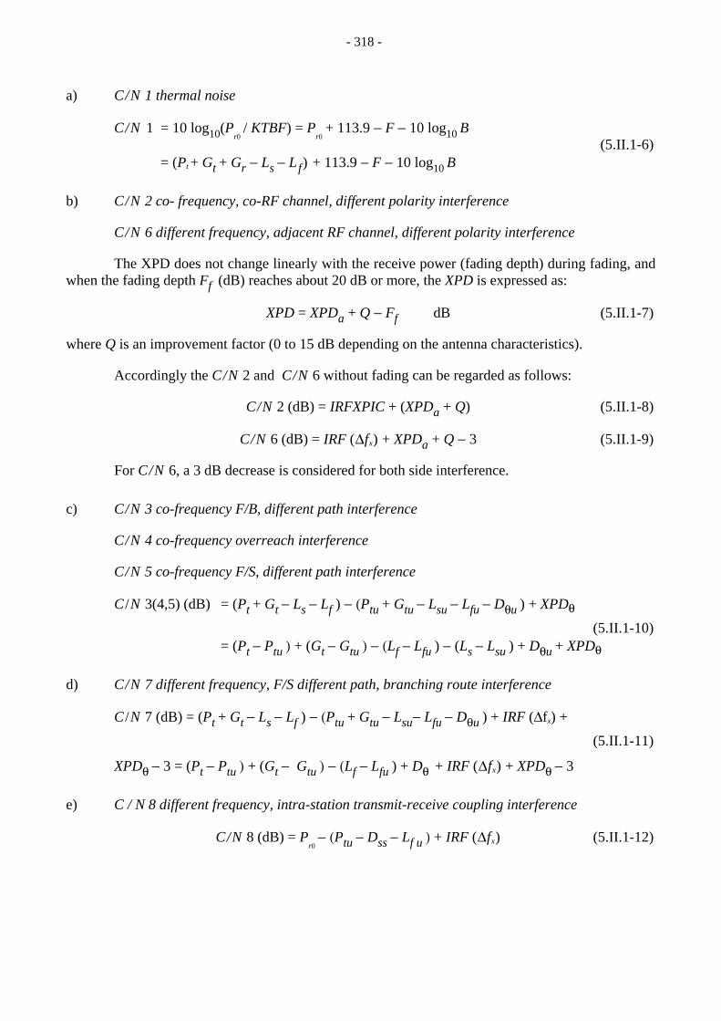
- 318 -

a) C/N 1 thermal noise

C/N 1 = 10 log10(Pr0

/ KTBF) = Pr0 + 113.9 − F − 10 log10 B

(5.II.1-6) = (Pt + Gt + Gr − Ls − Lf) + 113.9 − F − 10 log10 B

b) C/N 2 co- frequency, co-RF channel, different polarity interference

C/N 6 different frequency, adjacent RF channel, different polarity interference

The XPD does not change linearly with the receive power (fading depth) during fading, and when the fading depth Ff (dB) reaches about 20 dB or more, the XPD is expressed as:

XPD = XPDa + Q − Ff dB (5.II.1-7)

where Q is an improvement factor (0 to 15 dB depending on the antenna characteristics).

Accordingly the C/N 2 and C/N 6 without fading can be regarded as follows:

C/N 2 (dB) = IRFXPIC + (XPDa + Q) (5.II.1-8)

C/N 6 (dB) = IRF (∆fx) + XPDa + Q − 3 (5.II.1-9)

For C/N 6, a 3 dB decrease is considered for both side interference.

c) C/N 3 co-frequency F/B, different path interference

C/N 4 co-frequency overreach interference

C/N 5 co-frequency F/S, different path interference

C/N 3(4,5) (dB) = (Pt + Gt − Ls − Lf ) − (Ptu + Gtu − Lsu − Lfu − Dθu ) + XPDθ

(5.II.1-10) = (Pt − Ptu ) + (Gt − Gtu ) − (Lf − Lfu ) − (Ls − Lsu ) + Dθu + XPDθ

d) C/N 7 different frequency, F/S different path, branching route interference

C/N 7 (dB) = (Pt + Gt − Ls − Lf ) − (Ptu + Gtu − Lsu− Lfu − Dθu ) + IRF (∆fx) +

(5.II.1-11)

XPDθ − 3 = (Pt − Ptu ) + (Gt − Gtu ) − (Lf − Lfu ) + Dθ + IRF (∆fx) + XPDθ − 3

e) C / N 8 different frequency, intra-station transmit-receive coupling interference

C/N 8 (dB) = Pr0

− (Ptu − Dss − Lf u ) + IRF (∆fx) (5.II.1-12)

- 319 -

5.II.2 Dispersive fade margin based on normalized signature method

After the introduction of the equipment signature method described in the previous Annex 5.I, other approaches using a signature have been developed [Campbell and Coutts, 1982; Casiraghi and Mengali, 1987; Mojoli et al., 1989]. ITU-R has adopted Recommendation ITU-R F.1093 which summarizes the results of these studies. Features of the new methods are as follows. a) For broadband fading, occurrence factor P0 should be different to what is defined in

equation (5.I.2-2) or Chapter 4, equation (4.1.4-1). b) Instead of the signature product (w m), the values of the normalized signature Kn defined in

equation (5.I.3-5) are given for various modulation schemes.

c) Since it may be difficult to measure τm (mean value of the echo delay distribution) for all the radio hops, an approximation for τm using the hop length d (km) as a parameter has been proposed.

As given in Chapter 4, equation (4.1.4-21), the fade occurrence factor for broadband fading can be replaced with the following expression [Casiraghi and Mengali, 1987]:

P0d = η P0 = 1 − exp(−0.2 P0 0.75 )P0 (5.II.2-1)

where η is the reduction factor.

The relation P0d = P0 (η = 1) is also adopted in some countries as a worst-case prediction.

According to studies conducted in the 1980s [Casiraghi and Mengali, 1987; Mojoli et al., 1989; Damosso, 1985; Mojoro and Mengali, 1983], the following relationship for outage probability Pd is derived from Chapter 4, equation (4.1.4-22):

Pd = P0d CPb(1)·Kn<τ2> / T2 (5.II.2-2)

where: CPb(1) : constant factor related to the echo amplitude distribution Kn : normalized signature

<τ2> : second order moment of the echo delay distribution (ns) (see equation (5.I.3-3)) T : symbol rate period of the system (ns).

The value CPb(1) depends on the probability density function of the echo amplitude b. The calculated results for CPb(1) are given in Table 5.II.2-1.

TABLE 5.II.2-1

Values of CPb(1)

References [Campbell and Coutts, 1982]

[Mojoro and Mengali, 1983]

[Emshwiller, 1978; Damosso, 1985]

Pb (b) Uniform Exponential Weibull

CPb (1) 1.0 2.16 4.0

Pb(b) : assumed probability density function of echo amplitude.

The normalized signature Kn defined in equation (4.1.4-23) is given for each modulation scheme (see Table 5.II.2-2).

- 320 -

TABLE 5.II.2-2

Normalized signature

Modulation scheme Kn

64-QAM 15.4

16-QAM 5.5

8-PSK 7.0

4-PSK 1.0

For these values adaptive equalizers are not employed.

An approximation for <τ2> using correlation with the hop length d (km) has been proposed [Casiraghi and Mengali, 1987], as presented in Chapter 4, equation (4.1.4-24).

<τ2> = 2 τm2 = 2τm0 (d / 50)2 (5.II.2-3)

where:

τm : mean value of echo delay

τm 0 : reference value of τm for a 50 km hop

d : hop length

n : parameter depending on the propagation characteristics.

Proposed values for τm0 and n are given in Table 5.II.2-3.

TABLE 5.II.2-3

Values for τm0 and n

References [Campbell and Coutts, 1982]

[Mojoro and Mengali, 1983]

[Emshwiller, 1978; Damosso, 1985]

Pτ(τ) Exponential Exponential Exponential

τm0 1.0 ns 0.7 ns 0.5 ns

n 1.3-1.5

Pτ(τ) : assumed probability density function of echo delay.

In order to calculate Pd , we have to determine CPb(1), Kn, τm0 and n. The dispersive fade margin Fd is defined by:

Fd = − 10 log10 CPb(1)· Kn <τ2> / T 2 (5.II.2-4)

By using Fd and Ff , the total outage probability Pc is given by:

Pc = Pf + Pd = P0 ( 10−Ff /10 + η 10−Fd /10 ) (5.II.2-5)

- 321 -

5.II.3 Improvement of outage probability by countermeasures

5.II.3.1 General

Typical countermeasures used for outage improvement are space diversity, adaptive equalizers and interference cancellers. Their functions and improvement effects are described in the relevant sections of Chapter 4 (§ 4.3.6, 4.3.2 and 4.3.3, respectively).

Among the above countermeasures, space diversity improves both Pf and Pd in equations (5.II.1-5) and (5.II.2-2). On the other hand, adaptive equalizers are used for the improvement of Pd , and interference cancellers for the improvement of Pf by reducing a certain noise contribution.

The relationship between fade margin and outage probability during fading in DRRS with countermeasures can be represented by the curves shown in Fig. 5.I.5-1.

Improvement factors for space diversity are theoretically calculated in most cases; however, effects of adaptive equalizers or interference cancellers cannot be uniquely determined since the individual compensation performance is different. In the case of a normalized signature factor Kn the values in Table 5.II.2-2 are expected to become smaller by 1/10 to 1/20 in systems with modern transversal equalizers.

In this section, improvement factors for various countermeasures are presented for use by link designers.

5.II.3.2 Examples of improvement factors

5.II.3.2.1 Improvement of flat fade degradation a) Improvement factor with frequency diversity (Infd) [Vigants, 1975; Lee and Lin, 1985]:

If d

ffnfd

Ff

=⋅

⋅⎛⎝⎜

⎞⎠⎟ ⋅

0 810 10. ∆

(5.II.3-1)

where: f : band centre frequency (GHz) d : hop length (km)

(∆f/f) : relative frequency spacing as a percentage Ff : flat fade margin (dB).

The maximum Infd is limited to 5. b) Improvement factor with space diversity (Insd ) [Sadaki and Akiyama, 1979]:

Ifdnsd

Ff V

= ⋅⎛⎝⎜⎞⎠⎟ ⋅ ⋅ ×

−−S2 10 310 12 10. (5.II.3-2)

where:

S : vertical separation of receiving antennas, centre-to- centre (m)

V = | G1−G2 | where G1 and G2 are the gains of the two antennas.

The maximum Insd is limited to 200.

- 322 -

5.II.3.2.2 Improvement of dispersive fade degradation a) Improvement factor with frequency diversity (Idfd )

Idfd = 5 (constant) b) Improvement factor with space diversity (Idsd )

The outage probability with space diversity effect P 0 dd is given by the following formula:

PT

Kdd

n 0

04

212= ⎛⎝⎜

⎞⎠⎟ ⋅ ⋅

τ (5.II.3-3)

The improvement factor with space diversity is:

IP

P

TKdsd

d

dd

n=⎛

⎝

⎜⎜

⎞

⎠

⎟⎟ =

⎛⎝⎜

⎞⎠⎟ ⋅0

0 0

2 16τ

(5.II.3-4)

c) Improvement on dispersive fade degradation by equalizers (Ie )

Applying the parameter Kn given in Chapter 4, equation (4.1.4-22), the improvement factor of equalizers is obtained as follows:

( )

IK DEM

K DEM e n

ne =

for only(for with equalizers)

(5.II.3-5)

d) Synergistic effect [Meyer, 1984]

When both space diversity and equalizers are employed, a synergistic effect (ξ) can be expected as follows:

Id + e = Idsd ⋅ Ie ⋅ ξ (5.II.3-6)

Referring to [Tajima et al., 1983], ξ = Ie, then:

Id + e = Idsd ⋅ Ie 2 (5.II.3-7)

However, this result seems to be a little optimistic, judging from the field measurements.

Accordingly, one half of the synergistic effect is adopted as follows:

II I

d edsd e

+ =⋅ 2

2 (5.II.3-8)

General considerations on synergistic effects including experimental results are given in § 4.3.10.

5.II.4 General assessment procedure

Many parameters are discussed in Annexes 5.I and 5.II which deal with performance aspects of the link design. It may be helpful to clarify how these parameters relate to each other, and present a general work flow for the performance assessment of digital radio-relay systems. One example is given in Fig. 5.II.4-1.

- 323 -

FIGURE 5.II.4-1

Example of performance assessment procedure

- 324 -

ANNEX III TO CHAPTER 5

Performance prediction, method 3 (“linear amplitude dispersion” (LAD) statistics method)

5.III.1 Basis of the method

The LAD statistics outage prediction method was developed out of the observations and results of a 140 Mbit/s, 16-QAM digital radio field experiment which was conducted by the Research Laboratories of Telstra (formerly Telecom Australia) over the period November 1982 to April 1984. The radio equipment was operated in the 6.7 GHz band and was configured differently for each of the three years to allow different combinations of equalisation and diversity to be trialled. Descriptions of the equipment configurations and associated results were reported in [Martin et al., 1983; Campbell et al., 1984 and 1987].

The key conclusions of the field experiment provided the basis for the outage prediction method. In summary these were: – Digital radio outage occurs almost exclusively during periods of frequency selective fading

(FSF), which was defined as periods in which the pilot level of a working analogue system on the same path exhibited level enhancements.

– The severity of the FSF events to digital radio outage varied significantly. Defining the “intensity” of the digital radio outage without fading countermeasures as:

γ =System outage without countermeasures

Time FSF (5.III.1-1)

where Time FSF is the duration of the fading exhibiting frequency selective characteristics,

then over the three years of the field experiment γ ranged from 6 to 690 (outage s/h). Further, no strong correlation was observed between γ and the duration of the respective FSF event. Consequently, it was concluded that for the purpose of outage prediction separate consideration needs to be given to the duration of FSF and the severity of the FSF to digital radio performance. (As defined below, γ provides a measure of the mean echo delay.)

– The outage improvement factor obtained from adaptive amplitude equalisation (AEQ) demonstrated only a weak correlation with γ (reduced with increasing γ) and for most of the time was within the range 2 to 4. However, the outage improvement factor for space diversity was highly correlated with γ (reduced significantly with increasing γ). It was thus concluded that while equalisers can be well characterised by a constant improvement factor, such a concept is meaningless for space diversity (with or without equalisation).

– Because of the wideband nature of the digital signal, the statistics of the digital signal fade level during FSF generally will not follow the “10 dB per decade of probability” law, but rather falls away such that the probability of the deep fade decreases. The extent of the roll-off provides a measure of the channel dispersion statistics and can be used to estimate the mean echo delay.

- 325 -

– A significant year-to-year variation existed in the amount and severity of the FSF. This is seen to be true of all radio paths in general.

– The performance objective as defined in ITU-T Recommendations G.821 and G.826 is the most difficult to meet. Consequently, it was concluded that satisfying the performance objectives will ensure to a high degree of confidence that the associated availability objectives are met.

Like other reported outage prediction methods, the present method predicts the total time (s) due to inter-symbol interference (ISI) during which the system bit error ratio (BER) exceeds a given BER threshold (typically 10-3). A key outcome of the above conclusions is that the channel model used must possess the flexibility to model via parameters the effect of the severity of the FSF over a given time period (e.g. one month) on digital radio outage, and further, that the sensitivity of the radio equipment to FSF also be able to be expressed via parameters. A key feature of the developed outage prediction methods is that it also provides a framework by which arbitrary distributions of the channel parameters can be applied.

The outage probability from ISI is expressed as the product of the probability of FSF (η) and the probability of outage, given FSF (Ps | FSF):

( )P P FSFs s= η (5.III.1-2)

5.III.2 The fading model, parameter distributions and assumptions

The two-ray model is used to describe mathematically the radio channel for FSF. The channel function is expressed as:

( ) ( )( )[ ]C f a b j f f= − ⋅ − −1 2 0exp π τ (5.III.2-1)

where the channel parameters a, b, τ and f0 have their usual meaning [Coutts and Cambpell, 1982]. The notch frequency offset is denoted by F. For the prediction of outage from ISI the channel gain a is normalised to unity.

The two-ray model accommodates both minimum-phase (MP) state (b < 1) and non-minimum-phase (NMP) state (b > 1). As these conditions can impart a different performance on digital radio systems, (Ps | FSF) is expanded as:

( ) ( ) ( ) ( )P FSF P FSF P FSFs M s MP M s NMP= ⋅ + − ⋅η η1 (5.III.2-2)

where ηM is the probability of MP for FSF, and (Ps | FSFMP), (Ps | FSFNMP) are the outage probabilities for FSF, MP and MNP conditions respectively. ηM is usually assumed to be approximately 0.5 (for b approximately 1.0).

For the calculation of (Ps | FSFMP) and (Ps | FSFNMP) assumptions are required for the distributions of the two-ray model parameters. The outage prediction method recognises that the FSF characteristics of different radio paths will in general be different. This will also generally be true of the same radio path between different months or years. However, the outage probability for any radio path will be dominated by the severe fading events. With this understanding, statistical distributions are chosen which best capture the character of such fading periods. For this purpose the following distributions are assumed for both the MP and NMP conditions:

- 326 -

– Relative echo delay τ: negative exponential, possibly truncated (to negate unrealistic large delays), with the “mean echo delay” a parameter which reflects the severity of the FSF to digital radio outage:

( )Pk

eττ ττ

τ= ⋅

−Φ( ) /

00 0 0≤ ≤τ τk

– notch depth b: triangular distribution over the range 0 to 1:

( )P b bb = 2 for 0 1≤ ≤b

– Notch frequency offset F: uniform over the range -1/2τ to 1/2τ:

( )P FF = τ for − ≤ ≤12

12τ τ

F

5.III.3 Signature scaling and normalised system parameters

The approach of modelling the random nature of the echo delay necessitates a method to scale equipment signatures to other echo delays. For particular radio equipment which operates with baud period Tr, denote λc (F,τr,Tr) as the notch depth for outage (critical notch depth) at the notch frequency offset F and echo delay τr, where λ = 1 − b. λc (F,τr,Tr) thus represents the measured equipment signature and shall be termed the “reference signature”. The outage calculation requires the reference signature to be scaled to the echo delays over the distribution assumed. For the echo delay τ the following general scaling equation was proposed [Campbell and Coutts, 1982; Campbell, 1984]:

( ) ( )λ τ λ ττ

τ

β

c r c r rr

F T F T, , , ,= ⋅⎛⎝⎜

⎞⎠⎟

where β is chosen according to some rule, for example, that for a particular notch frequency offset the scaling gives the critical notch depth given from a second signature measurement at some echo delay different to τr [Coutts and Campbell, 1982]. A very convenient result appears if signatures are also scaled to unity baud period (in the units used, usually ns). This is achieved by applying a time scaling [Coutts and Campbell, 1982; Campbell, 1984]. Time scaling to the baud period T gives:

( )λ τ λ ττ

τ

β

c cr

r rr

rF T

TT

F TTT

, , , ,=⎛⎝⎜

⎞⎠⎟ ⋅⎛⎝⎜

⎞⎠⎟

(5.III.3-2)

Applying this scaling to the calculation of (Ps | FSF) yields a sequence of parameters which are given by an integral over the signature under the scaling of T = τ = 1.0 (ns units assumed):

( ) ( )Knc

F dF TT

F, ,T dFn rr

r

n

c r r= =⎛⎝⎜

⎞⎠⎟∫ ∫λ

τλ τ

β, . , .10 10 n = 1, 2, 3 .. (5.III.3-3)

- 327 -

Signatures with this normalisation have been called “normalised system signatures” while the parameters Kn have been called “normalised system parameters” [Campbell et al., 1987; Cambpell and Coutts, 1982; Campbell, 1984]. Because of the normalisation applied, the parameters Kn assume characteristic values dependent on the modulation method and equalisation used (see also ITU-R Report 784 (Volume IX, Part 1, 1990).

It should be understood that normalised system signatures are not measured signatures, and that the purpose for their introduction has simply been to provide a convenient means by which to describe the calculation of the normalised system parameters Kn. Also, the parameter β defines the rule for scaling the respective system signature to arbitrary echo delays. Thus the parameters Kn and β provide the characterisation of the radio equipment to two-ray fading.

As a consequence of equipment characteristics, for the same equipment different values of β may be appropriate for different ranges of expected echo delay. For example, without equalisation the scaling β = 1 has been found to be good for small delays, but for large delays β < 1 is often appropriate (typically 0.5 to 1.0). For this reason it is convenient to evaluate the parameters Kn for β = 1 then correct to other β values if appropriate later using the relationship:

K KT

n nr

r

n

β β β

β

τ= =

−

= ⋅⎛⎝⎜

⎞⎠⎟1

1( )

(5.III.3-4)

Values for K1 and K2 with β = 1 scaling obtained from signature measurements for various modulation methods (without equalisation) are presented in Table 5.III.3-1.

TABLE 5.III.3-1

Values for K1 and K2 (scaling β = 1) for various modulation methods without equalisation

Modulation method K1 K2

64-QAM 15.4 84.0

16-QAM 5.5 15.9

8-PSK 7.0 18.0

4-PSK 0.9 1.0

5.III.4 Outage prediction for non-diversity

The probability of outage (for both MP and NMP cases) is calculated as the probability that the state of the channel falls “under” the system signature.

For convenience the probability density function (pdf) of the echo delay is expressed as:

( )P fr ττ

ττ

=⎛⎝⎜

⎞⎠⎟

1

0 0 τ ≤ 0 (5.III.4-1)

- 328 -

where f (.) satisfies the properties of a pdf of unit mean and is characterised through the parameters cj,n defined by :

( )c f x n xnj, j d= ⋅ + ⋅∞

∫ ( ) exp β0

(5.III.4-2)

Further, the pdf of the notch depth λ, where λ = 1 − b, is defined through:

( )P ae

cn

λ

λ

λ λ λ0∫ ∑⋅ = ⋅d (5.III.4-3)

With the assumed uniform pdf for F the outage probability for ISI (MP or NMP case) becomes [Coutts and Campbell, 1982]:

( )P FSF a c KTS n

nl n n

n= ⋅ ⋅ ⎛

⎝⎜⎞⎠⎟∑

+

,τ β

01

(5.III.4-4)

The assumed pdfs for the notch depth gives a1 = 2, a2 = -1, while that for the echo delay with truncation at 5 times the mean (K = 5) gives c1,1 = 1.76, c1,2 = 4.45 with β = 1 scaling.

Predictions using this calculation have shown good agreement with measurements [Campbell et al., 1987]. Although not immediately apparent, an interesting result is that the predicted equaliser improvement decreases slightly with increasing mean echo delay, a result which was observed in the field experiment.

5.III.5 Outage prediction for diversity

For the calculation of outage from ISI with diversity (for both MP and NMP cases), the two-ray model is applied to each diversity branch. Each channel is thus described by the model parameters bi, Fi and τi for dual diversity i = 1,2. Individually, each channel is modelled statistically as that for non-diversity. To describe the interdependence between the diversity channels, it is hypothesised that the FSF on each diversity channel is the result of almost identical meteorological conditions, thus τ1 approximately equals τ2 and is denoted as τ, and that the channel parameters bi, Fi and τ are statistically independent. For dual diversity the outage probability for ISI is then [Campbell, 1984]:

( ) ( ) [ ]P FSF P d P F f F Fs divF

rF

− = ∫∫ ∫ττ

τ τ τ τ τ1

21 2

2

1 2,

, ,Outage d d d (5.III.5-1)

For baseband bit combining (BBC), for outage, both diversity branches must suffer outage simultaneously. The outage probability for ISI becomes [Campbell, 1984]:

( )P FSF a a .c K KTs div n m ,n m n m

mn

n m

− ⋅ + ⋅ ⋅+ +

= ⎛⎝⎜

⎞⎠⎟∑∑ 2 .

( )τ β0

2 (5.III.5-2)

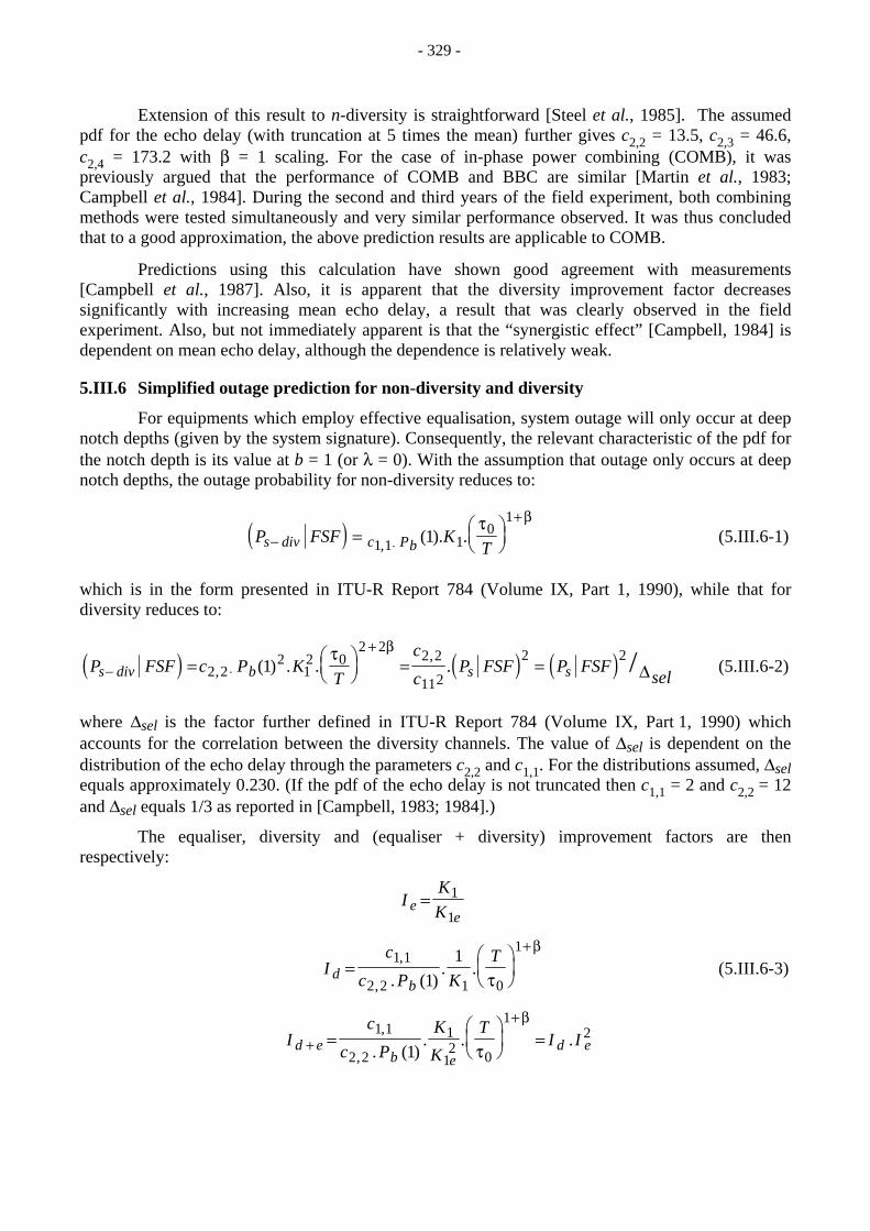
- 329 -

Extension of this result to n-diversity is straightforward [Steel et al., 1985]. The assumed pdf for the echo delay (with truncation at 5 times the mean) further gives c2,2 = 13.5, c2,3 = 46.6, c2,4 = 173.2 with β = 1 scaling. For the case of in-phase power combining (COMB), it was previously argued that the performance of COMB and BBC are similar [Martin et al., 1983; Campbell et al., 1984]. During the second and third years of the field experiment, both combining methods were tested simultaneously and very similar performance observed. It was thus concluded that to a good approximation, the above prediction results are applicable to COMB.

Predictions using this calculation have shown good agreement with measurements [Campbell et al., 1987]. Also, it is apparent that the diversity improvement factor decreases significantly with increasing mean echo delay, a result that was clearly observed in the field experiment. Also, but not immediately apparent is that the “synergistic effect” [Campbell, 1984] is dependent on mean echo delay, although the dependence is relatively weak.

5.III.6 Simplified outage prediction for non-diversity and diversity

For equipments which employ effective equalisation, system outage will only occur at deep notch depths (given by the system signature). Consequently, the relevant characteristic of the pdf for the notch depth is its value at b = 1 (or λ = 0). With the assumption that outage only occurs at deep notch depths, the outage probability for non-diversity reduces to:

( )P FSF KTs div c Pb− ⋅

+= ⎛

⎝⎜⎞⎠⎟1 1 1

01

1, ( ). .τ β

(5.III.6-1)

which is in the form presented in ITU-R Report 784 (Volume IX, Part 1, 1990), while that for diversity reduces to:

( ) ( ) ( )P FSF c P KT

c

cP FSF P FSF

sels div b s s− ⋅

+= ⎛

⎝⎜⎞⎠⎟

= =2 22

12 0

2 22 2

112

2 21,

,( ) . . . /τ β

∆ (5.III.6-2)

where ∆sel is the factor further defined in ITU-R Report 784 (Volume IX, Part 1, 1990) which accounts for the correlation between the diversity channels. The value of ∆sel is dependent on the distribution of the echo delay through the parameters c2,2 and c1,1. For the distributions assumed, ∆sel equals approximately 0.230. (If the pdf of the echo delay is not truncated then c1,1 = 2 and c2,2 = 12 and ∆sel equals 1/3 as reported in [Campbell, 1983; 1984].)

The equaliser, diversity and (equaliser + diversity) improvement factors are then respectively:

IKKe

e= 1

1

Ic

c P KT

db

=⎛⎝⎜

⎞⎠⎟

+1 1

2 2 1 0

1

11,

, . ( ). .

τ

β (5.III.6-3)

Ic

c PK

K

TI Id e

b ed e+

+=

⎛⎝⎜

⎞⎠⎟ =

1 1

2 2

1

12

0

12

1,

, . ( ). . .

τ

β

- 330 -

where K1e is that with equalisation. These equations give the equaliser improvement factor independent of the mean echo delay, but the diversity improvement factor inversely proportional to the mean echo delay to the power 1+ β. Also, the synergistic effect is given as the equaliser improvement factor.

5.III.7 Example application of the prediction method and comparison with measurements

Application of the prediction method to the field experiment system has been reported in [Campbell et al., 1987; Campbell, 1984] while that to a long overwater path with both dual and quad-diversity has been reported in [Steel et al., 1985]. In the latter case, outage probability measurements were used to estimate the mean echo delay experienced on the radio path, and this was then used to estimate the outage probability when quad-diversity is employed.

As an example application of the prediction method and comparison with measurements, the results and respective predictions for the 140 Mbit/s, 16-QAM digital radio field experiment are considered for the cases of no fading countermeasures (DEMOD), adaptive amplitude equalisation (AEQ), power combining (COMB), and adaptive amplitude equalisation with power combining (COMB+AEQ).

Signature measurements for the MP channel were available for the radio equipment under test. Denoting B(F) dB as the critical notch depth for the notch frequency offset F, Tr as the system baud period (28.6 ns for the test system) and τr the echo delay at which the signature is measured, then for the scaling β = 1, K1 and K2 are calculated as:

K TT

dF nn rr

r

nB F=

⎛⎝⎜

⎞⎠⎟ =−∫τ

10 1 220( ) / , (5.III.7-1)

The values obtained for K1 and K2 are given in Table 5.III.7-1. For the equipment under test the scaling β = 1 was found to be satisfactory. Under the distributions assumed, the simplified prediction equations presented above become:

( )P FSFs =⎛⎝⎜

⎞⎠⎟19 5

28 60

2

..

τ ( )P FSFs equ− =

⎛⎝⎜

⎞⎠⎟7 78

28 60

2

..

τ

(5.III.7-2)

( )P FSFs div− =⎛⎝⎜

⎞⎠⎟1 663

28 60

4τ.

( )P FSFs div equ− + =⎛⎝⎜

⎞⎠⎟264

28 60

4τ.

where the mean echo delay τ0 is in ns. From these results, the respective equaliser and diversity improvement factors and synergistic effect can be calculated.

TABLE 5.III.7-1

Values for K1 and K2 for the radio equipment under test

Equipment K1 K2

DEMOD 5.55 15.9 AEQ 2.21 4.36

- 331 -

The worst fading month over each of the three years of the field experiment, the propagation parameters η and τ0 were determined from the AGC and pilot level measurements of a working analogue system that operated on the same path. The results are given in Table 5.III.7-2.

TABLE 5.III.7-2

Propagation parameters for worst fading months

Year τ0 (ns)

η

1981-82 1.05 0.033 1982-83 1.84 0.068 1983-84 1.70 0.032

Using these parameters, the system outage time for the various equipment configurations was predicted. The results, together with the actual measured outages, are presented in Table 5.III.7-3.

TABLE 5.III.7-3

Comparison of measured and predicted system outages

Equipment 1981-82 1982-83 1983-84

Measured Predicted Measured Predicted Measured Predicted DEMOD 803 2 248 12 191 14 230 3 414 5 714

AEQ # 895 5 215 5 665 # 2 276 COMB # 258 4 034 5 021 684 1 722

COMB+AEQ 12 40 1 522 796 269 273

# : no measurement taken.

It is noted that the use of the simplified outage prediction equations lead to higher predicted outages than would be given by the general expressions presented.

5.III.8 Linear amplitude dispersion (LAD)/in-band (IBAD) method

5.III.8.1 Experimental validation of the method The benefits of using LAD or In-Band Amplitude Dispersion (IBAD) to provide a direct and simple graphical method of predicting outage have been discussed in the preceding sections. This section reports the results of field trial and laboratory measurements that validate the LAD prediction method and discusses some prediction method issues. In particular, the effectiveness of some implementations of modems and equalisers are sensitive to the % non-minimum phase.

5.III.8.2 Measured variations of LAD The first issue is to show from measurements that the LAD value holds constant over a range of propagation parameters and to verify that this value is a true characterisation of the modem only. The values of LAD or IBADT [Martin, 1987] were measured using a digital radio analyser over a range of delays and a range of non-minimum phase values. The percentage of non-minimum phase fading is important, as in the non-minimum phase channel the delayed ray arrives earlier than

- 332 -

the direct ray and to counter this effect the modem/equaliser should have a means of minimising same otherwise modem/equaliser performance will be degraded. This leads to the need to estimate the percentage non-minimum phase fading for modem/equalisers that are sensitive to this parameter. The fade simulator used for these measurements used a uniform distribution of notch frequency, a uniform distribution of the second ray amplitude and a maximum phase velocity of 0.6 π rad/s (300 MHz/s notch speed at 1 ns delay to 30 MHz/s notch speed at 10 ns delay) [Martin, 1987]. The results of this measurement for a modem are shown in Table 5.III.8-1

TABLE 5.III.8-1

Variation of LAD for different delays and percentage non-minimum phase

(For BER ≥ 10-3, 16-QAM, 140 Mbit/s modem without equalisers, LAD spacing = 30.0 MHz, S/N ratio > 60 dB)

Percentage non-minimum phase 1% 5% 10%

Delay (ns) (dB) (dB) (dB)

1 5.5 5.5 5.5 2 5.5 5.5 5.5 4 5.0 5.0 5.0 6 4.5 5.0 5.0 8 4.0 4.5 4.5

As can be seen from the above table the variation of LAD is minimal for a wide variation of delay and percentage non-minimum phase thus showing that LAD alone can be used to characterise a modem in dispersive fading. The decrease of the LAD value at high delays is due to the delay starting to become a significant fraction of the modem baud period.

Using the LAD value of 5.5 dB and applying it to data from a field trial [Campbell et al., 1987; Martin, 1984] yields the following predicted results which are compared with the actual results in Table 5.III.8-2.

TABLE 5.III.8-2

Predicted and actual seconds

(For BER ≥ 10-3, 16-QAM, 140 Mbit/s modem without equalisers, non diversity, LAD spacing = 30.0 MHz)

Event date Predicted using LAD

Actual

14 December 1983 576 967

18 December 1983 63 226

12 January 1984 1 576 2 192

TOTAL 2 215 3 385

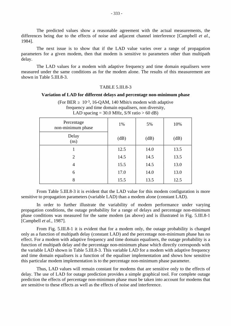
- 333 -

The predicted values show a reasonable agreement with the actual measurements, the differences being due to the effects of noise and adjacent channel interference [Campbell et al., 1984].

The next issue is to show that if the LAD value varies over a range of propagation parameters for a given modem, then that modem is sensitive to parameters other than multipath delay.

The LAD values for a modem with adaptive frequency and time domain equalisers were measured under the same conditions as for the modem alone. The results of this measurement are shown in Table 5.III.8-3.

TABLE 5.III.8-3

Variation of LAD for different delays and percentage non-minimum phase

(For BER ≥ 10-3, 16-QAM, 140 Mbit/s modem with adaptive frequency and time domain equalisers, non diversity,

LAD spacing = 30.0 MHz, S/N ratio > 60 dB)

Percentage non-minimum phase

1% 5% 10%

Delay (ns)

(dB) (dB) (dB)

1 12.5 14.0 13.5

2 14.5 14.5 13.5

4 15.5 14.5 13.0

6 17.0 14.0 13.0

8 15.5 13.5 12.5

From Table 5.III.8-3 it is evident that the LAD value for this modem configuration is more sensitive to propagation parameters (variable LAD) than a modem alone (constant LAD).

In order to further illustrate the variability of modem performance under varying propagation conditions, the outage probability for a range of delays and percentage non-minimum phase conditions was measured for the same modem (as above) and is illustrated in Fig. 5.III.8-1 [Campbell et al., 1987].

From Fig. 5.III.8-1 it is evident that for a modem only, the outage probability is changed only as a function of multipath delay (constant LAD) and the percentage non-minimum phase has no effect. For a modem with adaptive frequency and time domain equalisers, the outage probability is a function of multipath delay and the percentage non-minimum phase which directly corresponds with the variable LAD shown in Table 5.III.8-3. This variable LAD for a modem with adaptive frequency and time domain equalisers is a function of the equaliser implementation and shows how sensitive this particular modem implementation is to the percentage non-minimum phase parameter.

Thus, LAD values will remain constant for modems that are sensitive only to the effects of delay. The use of LAD for outage prediction provides a simple graphical tool. For complete outage prediction the effects of percentage non-minimum phase must be taken into account for modems that are sensitive to these effects as well as the effects of noise and interference.

- 334 -

0 1 2 3 4 5 6 7 8 9 10

100

10

1

0.1

0.01

0.001

Delay (ns)

Out

age

prob

abili

ty in

mul

tipat

h fa

ding

(%)

Modem only, 1 to 10%non-minimum phase

10% non-minimum phase



Modem plus adaptive frequency and time domain equalisers

FIGURE 5.III.8-1

Measured outage probability for a range of delays

(For a 16-QAM, 140 Mbit/s system in multipath fading. Fading simulator used a uniform distribution of notch frequency offset and a uniform distribution of second ray amplitude with a

maximum phase velocity of 0.6 π rad/s, S/N ratio > 60 dB)

- 335 -


CAMPBELL, J.C. [10 November, 1983] Digital radio outage prediction with space diversity. Electron. Lett., Vol. 19, 23.

CAMPBELL, J.C. [1984] Outage prediction for the route design of digital radio systems. Australian Telecommunication Research, Vol. 18, 2.

CAMPBELL, J.C. and COUTTS, R.P. [9 December, 1982] Outage prediction of digital radio systems. Electron. Lett., Vol. 18, 25, 1071-1072.

CAMPBELL, J.C., COUTTS, R.P., MARTIN, A.L. and REID R.L. [April, 1987] Observations and conclusions from a three year digital radio field experiment in Australia. IEEE JSAC, Vol. SAC-5, 3, 416-426.

CAMPBELL, J.C., MARTIN, A.L. and COUTTS, R.P. [1984] 140 Mbit/s digital radio field experiment – Further results. IEEE International Conference on Communications (ICC'84).

CASIRAGHI, U. and MENGALI, U. [1987] Comparison between some outage prediction methods for microwave digital radio. 17th European Microwave Conference, Rome, Italy.

COUTTS, R.P. and CAMPBELL, J.C. [1982] Mean square error analysis of QAM digital radio systems subjected to frequency selective fading. Australian Telecommunication Research, Vol. 16, 1.

DAMOSSO, E. [1985] Minimum and non-minimum phase fading effects on digital systems: a new approach to outage prediction. Proc. 4th International Conference on Antennas and Propagation (ICAP'85), Warwick, United Kingdom.

EMSHWILLER, M. [June, 1978] Characterization of the performance of PSK digital radio transmission in the presence of multipath fading. Conference Record, Vol. 3, 47.3.1-47.3.6. IEEE International Conference on Communications (ICC '84), Toronto, Canada.

GIGER, A.J. [1991] Low-Angle Microwave Propagation: Physics and Modeling. Artech House, Norwood, MA, United States of America.

GIGER, A.J. and BARNETT, T. [September, 1981] Effects of multipath propagation on digital radio. IEEE Trans. Comm., 1345-1352.

LEE, T.C. and LIN, S.H. [1985] A model of frequency diversity improvement for digital radio. Proceedings of ISAP’85, 509-512.

MARTIN, A.L. [13 September, 1984] Amplitude distortion: A means of characterising line-of-sight microwave radio paths during multipath fading. Electron. Lett., Vol. 20, 19, 798-799.

MARTIN, A.L. [April, 1987] Dispersion signatures, a statistically based, dynamic digital microwave radio measurement technique. IEEE JSAC, Vol. SAC-5, 3, 427-436.

MARTIN, A.L., COUTTS, R.P. and CAMPBELL, J.C. [1983] 140 Mbit/s digital radio field experiment. IEEE International Conference on Communications (ICC'78), Melbourne, Australia.

MEYER, M.H. [1984] Multipath fading outage estimates incorporating path and equipment characteristics. IEEE Global Telecommunications Conference (Globecom’84), 1466-1470.

- 336 -

MOJOLI, L.F., CASIRAGHI, U. and TOMATI, L. [1989] Design method for spectrum efficient digital TV transmission. Proc. 2nd European Conference on Radio-Relay Systems (ECRR'89), Abano Terme, Padua, Italy.

MOJORO, L. F. and MENGALI, U. [1983] Propagation in line-of-sight radio links. TELETTRA Review, Special Edition, Part II (Multipath Fading).

RUMMLER, W.D. [July, 1982] A comparison of calculated and observed performance of digital radio in the presence of interference. IEEE Trans. Comm., 1693-1700.

SADAKI, O. and AKIYAMA, T. [December, 1979] Multipath delay characteristics on line-of-sight microwave systems. IEEE Trans. Comm., Vol. COM-27, 12, 1876-1886.

SHAFI, M. and SMITH, P. [September, 1993] The impact of ITU-T Recommendation G.826. IEEE Communications Magazine.

STEEL, J., CAMPBELL, J.C. and DAVEY, L. [5 December, 1985] Measurement and prediction of digital radio performance on a long overwater path. Electron. Lett., Vol. 21, 25/26.

TAJIMA, K., KOMAKI, S. and OKAMOTO, Y. [May, 1983] Outage probability of a digital microwave radio equipped with space diversity and adaptive equalizer. Trans. IECE (Japan), Vol. J-66B, 5, 584-590.

VIGANTS, A. [1975] Space diversity engineering. BSTJ, 103-142.

BIBLIOGRAPHY

IVANEK, F. [1989] Terrestrial Digital Microwave Communications. Artech House, Norwood, MA, United States of America.

KURIHARA, N., KOBAYASHI, M. and ITO, K. [1982] 4/5/6 L-D1 field research results. Rev. Elec. Comm. Labs., Vol. 30, 5.

SIEMENS [1987] Equipment/system availability calculation in digital microwave radio systems. Siemens Publication.


Rec. ITU-R F.557 Availability objective for radio-relay systems over a hypothetical reference circuit and a hypothetical reference digital path.




- 337 -

Rec. ITU-R F.697 Error performance and availability objectives for the local-grade portion at each end of an ISDN connection utilising digital radio-relay systems.

Rec. ITU-R F.746 Radio-frequency channel arrangements for radio-relay systems.

Rec. ITU-R F.752 Diversity techniques for radio-relay systems.


Rec. ITU-R F.1093 Effects of multipath propagation on the design and operation of line-of-sight digital radio-relay systems.

Rec. ITU-R F.1094 Maximum allowable error performance and availability degradations to digital radio-relay systems arising from interference from emissions and radiations from other sources.

Rec. ITU-R F.1095 A procedure for determining coordination area between radio-relay stations of the fixed service.


Rec. ITU-R F.1097 Interference mitigation options to enhance compatibility between radar systems and digital radio-relay systems.

Rec. ITU-R F.1189 Error-performance objectives for constant bit rate digital paths at or above the primary rate carried by digital radio-relay systems which may form part or all of the national portion of a 27 500 km hypothetical reference path.

Rec. ITU-R P.530 Propagation data and prediction methods required for the design of terrestrial line-of-sight systems.

Rec. ITU-R P.837 Characteristics of precipitation for propagation modelling.

Rec. ITU-R P.838 Specific attenuation model for rain for use in prediction methods.

ITU-R Reports (1990)

Report 338 (Annex to Vol. V) Propagation data and prediction methods required for terrestrial line-of sight systems.

Report 784 (Annex to Vol. IX, Part 1) Effects of propagation on the design and operation of line-of-sight radio-relay systems.


ITU-T Rec. G.801 Digital transmission models.

ITU-T Rec. G.821 Error performance of an international digital connection forming part of an integrated services digital network.


- 338 -

CHAPTER 6

OPERATIONS AND MAINTENANCE

6.1 System maintenance and administration

6.1.1 Maintenance strategy

Degradations of performance of radio-relay systems occur consequences of ageing processes of radio-relay equipment, which, just as all other systems, require maintenance for keeping performance within defined limits according to relevant Recommendations adopted by ITU Sectors.

Globalisation of telecommunication networks now requires standardization of equipment used within the main process of signal transmission. The procedures to be performed in subordinate process of management, supervision and control of national and international networks have to be stimulated, taking into account a rapid transition in maintenance procedures from remote control/remote supervision to Telecommunications Management Network (TMN). This transition is mandatory for network operators in order to satisfy one of the main aspects of TMN: reduction of the delay between the occurrence of any event and the appropriate reaction to it in order to increase the availability of the connections.

6.1.2 Commissioning and acceptance tests

Commissioning and acceptance tests refer to the so-called “factory acceptance tests” and “field acceptance tests”.

Factory acceptance tests are performed at the supplier’s plant, where all test set-ups and means are available to verify that equipment ordered meets all the specifications agreed to in the contract. This control will be performed in common measurements by employees or commissioned persons of buyer and supplier respectively. It is thus ensured that equipment production was successfully finalized and equipment non-defective, prior to transportation to buyer’s stores. Cost and time effective reduction of these factory tests can proceed when “insurance quality procedures” (e.g., ISO 9000) are implemented by the supplier on its development and production line and are consequently applicable.

Field acceptance tests (FAT) are carried out by the supplier (manufacturer or distributor) in order to verify the proper operating conditions of the entities that he provides. These FATs result from the contract between the buyer (e.g. the network operator) and the supplier and therefore are not standardized by ITU.

Various administrative and technical measures are applicable to bringing-into-service (BIS) and maintenance operations, as later discussed. Such measures are distinct from FATs.

Difficulties in connection with acceptance tests may sometimes arise, as ITU Recommendations define error performance objectives for networks and links only, but they give no guidance related to equipment design objectives (see Fig. 6.1.2-1). It can be seen from the example given in this figure, that the Network Performance Objective (NPO) does not represent the figure to be checked in acceptance tests, because in test set-up measurements under simulated conditions, all interferences that are otherwise present under real environmental conditions and which cause unavoidable degradations, are missing. Main interferences originate from other radio-relay

- 339 -

equipment operating at the same frequencies and, for example, from the fixed-satellite service sharing fixed-terrestrial service’s frequency bands with equal priority. Details can be found in the ITU-R Report on performance limits for BIS and maintenance [ITU-R, 1996a].

Number of severely errored seconds in any month

Margin between networkperformance objective(NPO) and equipmentdesign objective (EDO) fornon-deterministic effects

Performance predictionexcluding interferencefrom the FSS

Total degradationallocated tointerference fromthe FSS (10%)

Increasing interference power (dB)

Network performanceobjective for hope.g. 36 SES

D01

FIGURE 6.1.2-1

Example of performance degradations due to the fixed-satellite service

Another difficulty in acceptance tests arises from the fact that error performance objectives defined by ITU-R Recommendations are “long term mean values” to be met within any month, but such periods of observation are not available in acceptance tests (see § 6.1.3.1).

Considering the above-mentioned time constraints and interferences affecting radio-relay systems via their receiving antennas, it might be concluded that Equipment Design Objective (EDO) (see Fig. 6.1.2-1) should be more stringent than NPO, although no safety margin has yet been recommended by the ITU-R. The margin should be agreed between buyer and supplier in their contract.

- 340 -

6.1.3 Bringing-into-service (BIS)

For the planning of digital hierarchy networks, the ITU-R has drawn up Recommendations regarding performance objectives for real digital radio-relay links; these objectives apply to a 64 kbit/s connection in accordance with ITU-T Recommendation G.821 (version 1990). These Recommendations are:

– Recommendation ITU-R F.634 for links in the high-grade portion of international links;

– Recommendation ITU-R F.696 for links in the medium-grade portion (national links);

– Recommendation ITU-R F.697 for the local-grade portion at each end of the connection.

ITU-R Recommendations based on the new version of ITU-T Recommendations G.821 and G.826 have been established for bit rates at or above the primary rate (1.5 Mbit/s, 2 Mbit/s or above). These Recommendations are dedicated to the Hypothetical Digital Reference Path (HDRP); ITU-R Recommendations for radio-relay digital path based on ITU-T Recommendation G.826 are Recommendations ITU-R F.1092 (international portion) and ITU-R F.1189 (national portion). Others may be established in the near future.

In addition, ITU-T Recommendations M.2100 (for Plesiochronous Digital Hierarchy (PDH)) and M.2101 (for Synchronous Digital Hierarchy (SDH)) give a method of calculating error performance thresholds for BIS and maintenance of digital transmission systems.

On the basis of the above-mentioned Recommendations, this section describes a method for identifying performance objectives to be respected at the system bit rate, applicable for BIS and maintenance of digital radio-relay systems used in PDH and SDH [ITU-R, 1996a].

ITU-R is currently studying a new Recommendation, aligned to ITU-T Recommendation G.826, which will cover PDH, SDH and cell-based paths at primary rate level and above for BIS.

For the sake of consistency with ITU-T Recommendations M.2100 and M.2101, only the parameters ES and SES will be used in setting the performance limits for BIS and maintenance of digital radio sections, that is:

– ES (Errored Second ): period of 1 s with one or more bit errors.

The sensitivity of the ESd (one single bit error is sufficient to cause an ESd) makes it a highly suitable parameter for checking the performance of radio-relay sections during BIS and maintenance;

– SES (Severely Errored Second): a 1 s period which contains ≥ 30% errored blocks or at least one defect, for instance frame synchronization loss(es) detected or the transmission of the Alarm Indication Signal (AIS) (a list of defect conditions is included in ITU-T Recommendation G.826 for SDH systems).

NOTE 1 – The abbreviations ESd and SESd, with a “d”, are used to designate performance limits which are specific of the system bit rate.

6.1.3.1 Reference performance objectives

The proposed method for setting up the different performance limits is derived from ITU-T Recommendations M.2100 and M.2101 and is based on the Reference Performance Objectives (RPO). The RPO may be expressed in terms of errored seconds at the system bit rate (i.e. RPO (ESd)) and severely errored seconds at the system bit rate (i.e. RPO (SESd)) (see § 3.2.4).

- 341 -

The limits applicable to BIS and maintenance are based on measurement periods much shorter than one month. These short periods are assumed not to be significantly affected by adverse propagation. Thus, the end-to-end RPO values identified in Table 3.2-4, extracted from ITU-T Recommendation M.2100, do not take into account the additional allocation for adverse propagation conditions given in relevant ITU-R Recommendations.

The ITU-T Recommendations M.2100 and M.2101 have defined RPO at or above the primary rate which is derived from ITU-T Recommendation G.826. Work to adopt these Recommendations to digital radio-relay systems is currently under progress within Radiocommunication Study Group 9; this work will result in Recommendations defining performance limits for BIS and maintenance for digital radio-relay systems operating in PDH and SDH based international paths and sections.

A part of the global RPO is allocated to each Path Core Element (PCE) being part of an international path or section. The allocation is attributed according to the distance as defined in ITU-T Recommendations M.2100 and M.2101. RPO and its allocation are reported in Tables 3.2-3 and 3.2-4.

The DRRSs have to be designed in such a way that the PCEs of which they take part satisfy these objectives. Objectives of error performance for BIS and maintenance of real DRRSs should be defined accordingly.

6.1.3.2 BIS limits

Performance limits should be used as an objective during BIS and for maintenance periods. These procedures are intended to result in network performance compliant with the objectives of ITU-T G-Series Recommendations. Practical considerations require that BIS and maintenance limits be based on shorter test periods (i.e. shorter than 1 month) which correspond to the test period for long-term performance objectives.

In § 3.2.4-1 it was mentioned that statistical fluctuations in the occurrence of anomalies and defects means that we cannot be certain that long-term objectives are met. The limits of the numbers of events and the duration of measurements attempt to ensure that systems or paths exhibiting unacceptable or degraded performances can be detected. The only way to ensure that a system or path meets network performance objectives is to do continuous measurement over a long period (i.e. months), but the definition of margins for BIS period measurement ensures a high level of confidence that the long-term objectives will be encompassed by the path or section. This margin provides for both ageing and severe propagation conditions. The way to cope with severe fading conditions during BIS procedure is under study in Radiocommunication Study Group 9 with the assistance of Radiocommunication Study Group 3. Limits are needed for several maintenance functions as defined in ITU-T Recommendation M.20. This Recommendation provides limits for three of these functions:

– BIS,

– keeping the network operational (maintenance),

– system restoration.

Once radio-relay links have been placed into service, network supervision requires operational/maintenance limits, as described in ITU-T Recommendation M.20. Such supervision is done on an in-service basis using performance monitoring equipment. The supervision process involves analysing anomalies and defects to determine if the performance level is normal, degraded

- 342 -

or unacceptable. Thus, degraded and unacceptable performance limits are required. In addition, a limit on performance after repair is also required which may differ from the BIS limits.

6.1.3.3 Calculation of BIS limits

The BIS testing procedure is defined in ITU-T Recommendation M.2110, and is under study by Radiocommunication Study Group 9 [ITU-R, 1996b]. The derivation of the limits is a function of a given allocation and test period and based on a pragmatic rule. As explained in § 6.1.3.1, these limits depend on the parameters and objectives of ITU-T Recommendation G.826.

The difference between RPO and BIS limits is called the ageing margin. This margin should be as large as possible to minimize maintenance interventions. Practical values may be chosen from RPO/10 to RPO/2.

Two limits, S1 and S2, are provided for use in short-term BIS testing, as shown in Fig. 6.1.3-1. If performance is better than the first limit S1, the entity can be brought into service with some confidence. If performance is between the two limits, further testing is necessary and the entity can only be provisionally accepted. Corrective action is required if performance is worse than the second limit S2.

D

D

S2

S1

T0403830-93/d05

The objectiveis likely to be

satisfiedBringing-into-

service accepted

Bringing-into-service aborted

uncertainty

No. of events

BIS objective(RPO/2)

Provisionalbringing-into-service

andfurther testing

The objectiveis unlikely to be

satisfied

FIGURE 6.1.3-1

Bringing-into-service limits and conditions

The ageing margin for transmission systems depends on the procedures of each administration (Buyer). A stringent limit which is RPO/10 should be used when previous commissioning tests have not been carried out.

The methodology of calculation of BIS performance limits can be found in [ITU-R, 1996b], Annex, titled “Performance limits and methodology for BIS”.

If commissioning tests have been made before BIS measurement, the out-of-service tests for BIS can be carried out for a shorter period and do not require the same stringent limits.

- 343 -

The practical process for BIS measurement for path elements including DRRSs is under study at ITU-R. As an example, the procedure defined by the ITU-T Recommendations M.2100 and M.2101 is reported below. The adequacy of this procedure to DRRSs is under discussion.

The practical BIS procedure may be split into two steps. In an initial 15 min period, Out-of-Service Measurement (OSM) of the link to be brought into service shall be loaded by an appropriate Pseudo-Random Binary Sequence (PRBS) signal. During this period, no error or unavailability event should occur. This step must be repeated up to two times, if any event is observed. If there is any event during the third (and last) test, the BIS procedure for fault localization and correction shall be interrupted.

After successfully passing the first step, a 24-h test is applied. Real traffic could be carried on the path, if In-Service Measurement (ISM) is applicable, or the test is applied again using a PRBS signal as in the previous test. Should an unavailability event occur during the BIS testing, the cause should be investigated and a new BIS test re-scheduled. Should a further unavailability event occur in the second test, the procedure should be postponed until the origin of the irregularity has been cleared.

At the end of the 24-h period, the results of the measurement are compared to the BIS limits S1 and S2. Depending on the results of the tests (ES, SES or both, are below the limit values S1, between S1, S2 or outside S2) different scenarios are possible. Decisions to be derived from test results may be:

– acceptance of the path,

– provisional acceptance of the path, but subject to an extended 7-day BIS testing period,

– rejection and entry into the fault localization/maintenance mode.

For routes with new equipment, a 7-day test should be used and performance must satisfy the BIS 7-day limit for each parameter (ES or SES).

Further details are given in ITU-T Recommendation M.2110 and [ITU-R, 1996a and b]. Continuous in-service monitoring is required to provide sufficient confidence on the long-term performance.

6.1.4 Maintenance

This section reports on the limits and procedures which are defined in ITU-T Recommendations M.2100, M.2101, M.20 and M.34. Their suitability to radio links is currently under study in Radiocommunication Study Group 9.

A progressive degradation of the equipment performances of digital radio-relay systems will usually not cause errors or raise any alarms but will reduce the available fade margin. Thus, in normal free-space propagation conditions, the system will continue to operate with no errors despite the progressive degradation. During fading, however, greater outages will result from the degraded threshold. To be protected against such effects, appropriate maintenance efforts are necessary so that maintenance personnel become aware of equipment degradations.

It should be noted, that different administrations/authorities/network operators will employ different criteria to supervise their network, to initiate the maintenance periods, and will have their own methods regarding required data and in what way they should be communicated to neighbouring monitoring stations in international connections.

To make easier maintenance processes by means of forthcoming Telecommunications Management Networks (TMNs) it is highly desirable to standardize datas, equipment, interfaces, protocols etc. related to this matter.

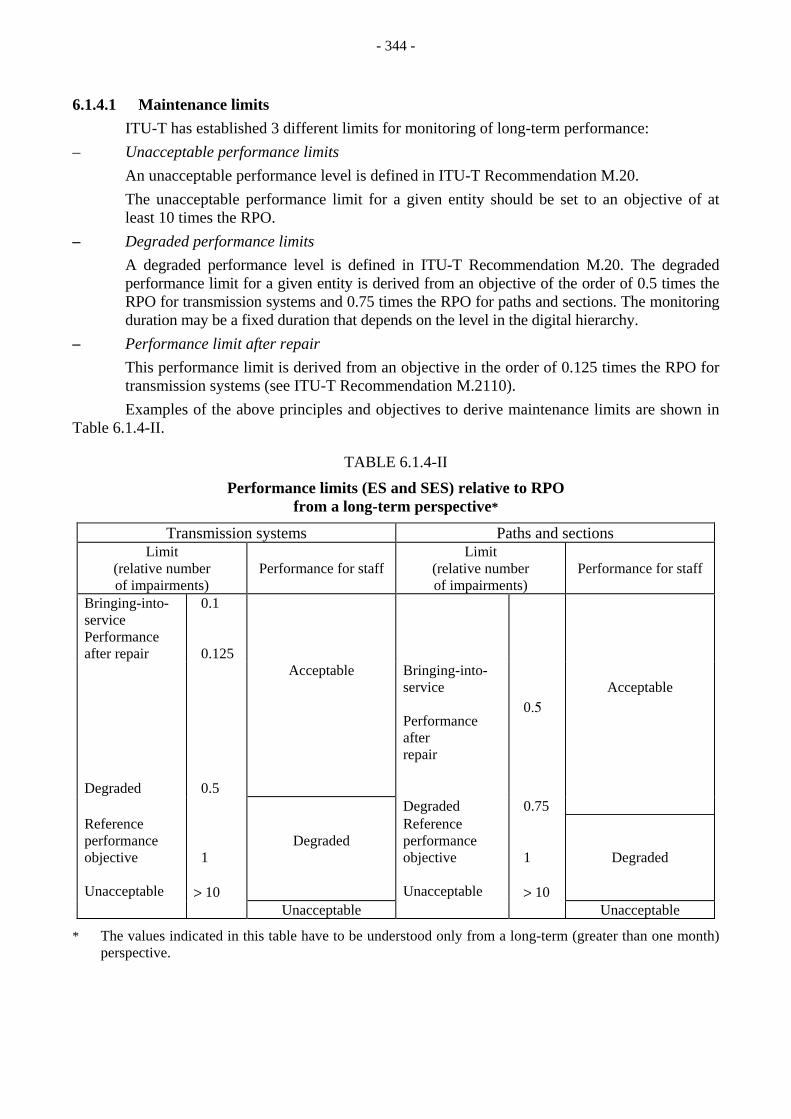
- 344 -

6.1.4.1 Maintenance limits ITU-T has established 3 different limits for monitoring of long-term performance: – Unacceptable performance limits An unacceptable performance level is defined in ITU-T Recommendation M.20. The unacceptable performance limit for a given entity should be set to an objective of at

least 10 times the RPO. – Degraded performance limits A degraded performance level is defined in ITU-T Recommendation M.20. The degraded

performance limit for a given entity is derived from an objective of the order of 0.5 times the RPO for transmission systems and 0.75 times the RPO for paths and sections. The monitoring duration may be a fixed duration that depends on the level in the digital hierarchy.

– Performance limit after repair This performance limit is derived from an objective in the order of 0.125 times the RPO for

transmission systems (see ITU-T Recommendation M.2110). Examples of the above principles and objectives to derive maintenance limits are shown in Table 6.1.4-II.

TABLE 6.1.4-II

Performance limits (ES and SES) relative to RPO from a long-term perspective*

Transmission systems Paths and sections Limit

(relative number of impairments)

Performance for staff

Limit (relative number of impairments)

Performance for staff

Bringing-into-service

0.1

Performance after repair

0.125

Degraded

0.5

Acceptable

Bringing-into-service Performance after repair

0.5

Acceptable

Degraded 0.75 Reference performance objective Unacceptable

1 > 10

Degraded

Reference performance objective Unacceptable

1 > 10

Degraded

Unacceptable Unacceptable

* The values indicated in this table have to be understood only from a long-term (greater than one month) perspective.

- 345 -

The general strategy for the use of performance monitoring information and thresholds is described in ITU-T Recommendations M.20 and M.34. These thresholds and information will be reported to operations systems via the TMN for both real time and longer term analysis. When thresholds of unacceptable or degraded performance levels are reached, maintenance action should be initiated.

6.1.4.2 Fault detection and localization

All possible BIS and maintenance activities are based on satisfying/exceeding defined limits of performance related to RPOs. This concept requires that bit errors be recognized by means of error detection monitors having a minimum error detection capability > 90% (see ITU-T Recommendation G.826). Evaluation of error performance parameters ES and SES is based on standardized signals using “anomalies” and “defects”, the concepts of which are defined in ITU-T Recommendation M.20.

Details connected to the field of measuring error performance parameters of digital radio-relay systems are dealt with in § 6.2 of this Handbook.

TMN, as described in ITU-T Recommendation M.30, is being progressively implemented by many administrations. The maintenance procedures described here cover both the case where full In-Service Measurement (ISM) is available (as in the TMN) and the case where no ISM or partial ISM is available. The latter case is referred to as pre-ISM.

Information processing will then be more integrated or less integrated depending on the TMN’s degree of development.

ISM should be understood as a situation where a dedicated performance monitor exists for each path and transmission system. This facilitates performance data collection, setting thresholds, and filing historical performance data in archives.

A pre-ISM situation exists if any condition does not meet the definition of ISM (e.g., existence of time shared monitoring or no monitoring at all). The concept of “network elements” then allows a “local operation” of a radio-relay section using all technical means of inherent remote control/remote supervision equipment installed at a monitoring station to identify any kind and location of a fault.

6.1.4.3 Fault localization information

Once an alarm indication is received under ISM-conditions, the fault localization process must begin. For this purpose several categories of information are required:

– performance information,

– performance level information,

– primitive performances,

– any additional information.

Performance level information (unacceptable performance level, degraded performance level, normal performance level) is derived from performance information (or the equivalent primitive performances). This is the information which will start the alarm information process shown in Fig. 6.1.4-1 (see ITU-T Recommendation M.2120) when a performance limit is reached. The performance limits are also referred to as alarm thresholds. The alarm generated (i.e. prompt maintenance alarm, delayed maintenance alarm or maintenance event information), determines the urgency of consequent actions.

- 346 -

T0403860-93

Performanceinformation

SEF MEF Othersources

Level of performance

Alarminformation

process

Maintenance process

Supplementaryinformation

Performanceevaluation

Figure 9/M.20 [6]

Performanceprimitives

Defectsupervision

process

Supervisionprocess foranomalies

Figure 7/M.20

FIGURE 6.1.4-1

Process of elaboration of information used for maintenance

SEF: Support Entity Function MEF: Maintenance Entity Function

Primitive performances are the basic information in the form of anomalies and defects used to determine the parameter counts of ITU-T Recommendation M.2100. Primitive performances depend on the type of monitored entity.

Additional information is information other than that obtained from monitoring. It includes derived information such as the identification of a faulty equipment or sub-entity. It also includes administrative information such as the structure of a path or the availability of means of direct transmission restoration (protection switching).

- 347 -

All of this information is needed to initiate suitable measures by maintenance staff to restore the “normal operation” of the considered paths. The data (time of occurrence, duration etc. ...) of error performance parameters ES and SES and periods of unavailability should be stored to form a basis for further analysis.

In order to provide a better service to customers, many administrations use, or intend to use, a preventive approach for maintenance and fault localization. Preventive maintenance implies locating and correcting faults before a performance impairment reaches an unacceptable or degraded performance level.

Among available tools for preventive maintenance, the “trend” analysis can be used. Information is gathered from several points in the network, date/time-stamped and stored. Continuous automatic comparisons of measurements from a particular point may indicate by the trend of the measurements that there is a potential fault. The results of the trend analysis may generate the equivalent of a low level deferred maintenance alarm. Economic studies will determine at what point an administration may decide to apply this action.

An indication which may be useful in the trend or comparison analysis is error performances. A path or section which has poorer error performance than similar paths or sections, or which is showing a trend of increasing errors, may become the target of reinforced maintenance.

Trend analysis of this type implies a well developed TMN with wide deployment of ISM techniques.

6.1.4.4 Fault localization procedures on digital transmission system

Fault localization on digital transmission systems largely depends on the fault localization means available to the monitoring station. However, the following guidelines can be used.

Fault localization in a pre-ISM environment

In a pre-ISM environment, a transmission system may not yield standardized parameters and may not have the capability to record performance history. In this situation the only opportunity is to monitor the faulted link after the event on a forward-going basis, using an appropriate test equipment.

This process cannot guarantee the identification of the source of the original performance problem, particularly if it is of a transient nature.

The monitoring station in charge of the faulty path should:

– determine the path routing;

– split the path into sections. If traffic is not totally interrupted, an in-service measuring instrument as described in ITU-T Recommendations O.161 and O.162 should be placed at various accessible points along the path to determine which part is at fault. These measurements are made at protected monitoring points;

– coordinate the measurement process in such a way that subcontrol and participating centres start and stop their measurements at the same time;

– centralize results, either at the control station or at the fault report point, and compare to determine the faulty section;

- 348 -

– ensure that there are no monitoring “blind spots” on the path. A “blind spot” is a portion of the path which exists between two monitored sections. As an example, cross-connect equipment may not be covered by the monitors of the transmission systems connected to the input and the output. Unless such a cross-connect has its own monitoring system, it may be overlooked.

If several sections are in fault, the fault localization will normally concentrate first on the most severely degraded section. Where additional maintenance effort is available, the total out-of-service (OOS) time may be reduced by utilizing this additional effort on less degraded sections. However, control is needed so that the efforts of the technical staff in charge do not mask a problem being worked on by another.

If the traffic is totally interrupted, or ISM instruments are not available, the same fault localization procedure as before will be used, but entering a pseudo-random bit sequence.

The input points and the monitoring locations should be chosen for efficiency of localization. This includes the possibility of loopback.

Fault localization in an ISM environment

The monitoring station of the path is informed of problems by unacceptable or degraded performance level information, trend analysis, and/or by a user’s complaint.

When such performance level is reached, the following should be carried out:

– immediately send a message to the control stations of the paths carried by the transmission system;

– store the message for access by those control stations which do receive the message directly. The storage will normally be at the fault report point;

– initiate the fault localization capability of the Maintenance Entities (MEs) to find the faulty maintenance sub-entity. This should be done in a time frame appropriate to the prompt or deferred maintenance alarm levels;

– undertake corrective action in a time frame appropriate to the alarm level (prompt or deferred maintenance alarm or special instructions);

– confirm the unacceptable or degraded level of the path by consulting the history of the path (BIS data, daily book etc.).

Once the above-mentioned procedures are initiated, the control station of the ME concerned is expected to provide supplementary information to the TMN data base.

The control stations of paths supported by the ME will be able to determine from the data base such information as the expected return into service time, taking into consideration information on any other faulty MEs which affect the path.

If the above-mentioned procedure cannot be implemented, path routing should be determined and the higher level path control stations questioned for determining the origin of the fault. This interrogation can be carried out directly or by consulting data bases. The information exchanged must be expressed in terms of performance information as indicated in ITU-T Recommendations M.2100 and M.2101, with all events date/time-stamped, and the affected direction

- 349 -

indicated. This procedure must lead to assigning the problem to the ME control station where the degradation exists.

When the repair action on a faulty ME is completed, an appropriate assurance of satisfactory performance should be made.

Depending on the type and the origin of the fault and the repair process, this assurance may be as simple as the ability to carry a signal, or may be more complex.

When the path is returned to service it should be monitored on a reinforced basis. By analogy with the values of Performance Limits for BIS (PLBIS) corresponding values of Post-Maintenance Performance Limits (PMPL) should apply ( the values given below are provisional):

PMPL = 0.125 x APO for PDH Transmission Systems or SDH Multiplex Sections

= 0.5 x APO for PDH and SDH Paths or SDH Sections

where APO: Allocated Performance Objective

6.1.5 Alarms

Alarms are considered as a means to indicate to maintenance staff any deviation from a state of normal operation. Supervision of DRRS is therefore mandatory in order to operate a network on a level of performance required by buyers and defined by relevant ITU Recommendations. Early discovery of failures and appropriate counteractions are required. Information on the faulty equipment, the degraded or even unacceptable performances, will be transmitted to the supervisory or control centre and weighted due to their urgency.

6.1.5.1 Alarms under pre-ISM conditions

A digital radio-relay system is usually equipped with supervision/monitoring facilities in order to help maintenance staff in the following actions:

– rapid localization of a fault which has interrupted traffic on a channel (type a): prompt alarm),

– detection of signal degradations (type b): deferred alarm).

Alarms arising from type a) events, are considered as “prompt” alarms, but type b) events will initiate “deferred” alarms. Built-in supervision modules will automatically detect such events, activate both local visual indicators and alarm signal generators to extend the alarm to a supervisory station.

It is a special feature of DRRS that alarms due to unacceptable BER may occur during adverse propagation conditions when there is no fault in the equipment itself. “Corrective action” is therefore not relevant. To determine the true source of an alarm, additional criteria providing propagation information (automatic gain control voltage, activity of time-domain equalizers if any) should be analysed, bearing in mind that the duration of adverse propagation conditions may last between a few seconds and several hours.

Plesiochronous DRRS will generally generate maintenance alarm signals on both terminals:

– transmitter side in case of loss of baseband signal at the modulator input and due to equipment faults,

- 350 -

– receiver side in case of BER >10-3, loss of frame (LOF), loss of channel identification and equipment faults.

In these cases DRRS will transmit in downstream direction, instead of interrupted traffic, an Alarm Indication Signal (AIS), give in upstream direction an Upstream Failure Indication (UFI) and initiate a service alarm to the monitoring station.

As is noted by ITU-T, AIS should be sent immediately (e.g. in a few ms) after detection with appropriate confidence of a fault condition. In order to avoid frequent insertion and removal of AIS, it is necessary to verify the persistence of the fault condition (e.g. high error ratio) for a longer time interval. In any case, the AIS should be sent within 500 ms after the beginning of the fault conditions, including detection time.

All demultiplexers are able to identify AIS and receive in this way the information that a fault occurred in a previous network element. Thus generation of AIS by all subsequent demodulators/demultiplexers on lower order paths is avoided.

6.1.5.2 Alarms under in-service measurement (ISM) conditions

ISM is understood as a situation where a dedicated performance monitor exists for each path and transmission system. This facilitates performance data collection, setting thresholds and filing historical performance data in archives (see ITU-T Recommendation M.2120). This situation is given when TMN is fully implemented in a SDH-network and maintenance will function on principles defined in ITU-T Recommendations of the M.20 Series. All criteria, information, data and voice channels for maintenance and management of a modern SDH-network are available in the SOH of the STM-N signal. The great volume of information to be exchanged and processed can be handled by computer-assistance only.

Any performance information will start the alarm information process as shown in Fig. 6.1.4-1 when a performance limit (= alarm threshold) is exceeded. The alarms then generated are categorized as (see ITU-T Recommendations of the M.20 Series):

a) Prompt Maintenance Alarm (PMA)

A prompt maintenance alarm is generated in order to initiate maintenance activities (normally immediately) to remove from the service a defective equipment and for the purpose of restoring good service and effecting repair of the failed equipment.

b) Deferred Maintenance Alarm (DMA)

A deferred maintenance alarm is generated when immediate action is not required, e.g., when performance falls below standard but the effect does not justify removal from the service, or generally if automatic changeover to standby equipment has been used to restore service.

c) Maintenance Event Information (MEI)

This information has to be generated as a consequence of events when no immediate actions are required because the total performance is not degraded. The maintenance actions can be performed on a scheduled basis, or after the accumulation of maintenance event information indications.

- 351 -

Both the malfunction supervisory process and the alarm information process, including the use of PMAs, DMAs and MEIs, can also be applied to other non-telecommunications equipment (e.g. power, diesel generators, temperature control, etc.).

The failure information at the alarm interface is used to determine the faulty maintenance entity or part of the maintenance entity. The information can be presented either locally, or remotely via an alarm collection system.

The great amount of alarm signals that may exist in extended DRRS forming one Network Element (NE) (including for example up to 10 hops in tandem and 10 channels in parallel) decisively assist operation of the network and help to find the place and the real cause of faults. At the same time they give necessary information to all services/supervisory centres of lower order paths thus avoiding useless maintenance efforts. Examples of the great variety of SDH-alarm signals are:

– LOS Loss of Signal: initiated by a demodulator in case of receiver input levels below a threshold value causing BER >10-3. The LOS state is left when two consecutive error-free frame alignment signals have been received.

– OOF Out of Frame: the signal is generated after having received four or five consecutive erroneous Frame Alignment Word (FAW). The alarm signal OOF disappears after detection of two consecutive valid FAW.

– LOF Loss of Frame: this signal is generated when OOF is present for more than some ms. It is proposed to define the appropriate time within a period < 3 ms.

– LOP Loss of Pointer: the signal is generated after having received 8 to 10 erroneous pointer signals. The reception of 3 consecutive correct pointer signals is sufficient to delete LOP indication.

These basic alarms are accompanied in SDH-systems by many additional alarms sent in up-/downstream directions to indicate with more details the nature of failures and thus enabling a TMN to monitor NE failures nearly in real time. The received TMN weighting alarm information determine the nature and severity of a fault and its effect on the services supported by the faulty equipment.

6.1.6 Service channels

Recommendation ITU-R F.753 gives in its Annex, § 4, three proposals to provide service channels:

a) transmission by inserting supervision and control signals into the main signal pulse sequence, e.g. Radio Frame Complementary Over-Head (RFCOH). Providing service channels in this way will produce no degradation of the main signal and forms an economical way to utilize the capacities of DRRS. Some administrations built up in this way 2 Mbit/s channels in parallel to long-haul trunk traffic to meet local/regional requirements (way-side traffic);

b) transmission separately from the main signal pulse sequence. This includes the use of additional modulation of the main carrier;

- 352 -

c) transmission means other than the main signal path.

For supervising and controlling intermediate repeater stations and to meet the needs of maintenance staff, insertion and detection of the supervision and control signal and at least of one Engineering Order Wire (EOW) channel for voice communication must be accomplished at each station.

The second method proposed in b) above can be suitable in some cases for the transmission of small capacity supervision and control signals. In particular, additional FSK or FM modulation of the main carrier is suitable for supervision and control signal transmission, because these modulation methods typically exhibit longer transmission availability than the main signal, during fading conditions. However, the upper limitation of transmission capacity depends on the main signal modulation method and supervision and control signalling pulse shape.

Considering the implementation of radio systems in SDH networks, the supervision and control signal transmission method given below should also be taken into account.

Forward Error Correction (FEC) may be used to achieve high quality in multi-state modulation. In radio-relay systems installed with FEC, it is possible to synchronize supervision and control signals at regenerator stations without special frame signals and to transmit them. This is achieved by the access to the additional supervision and control bits that are added by the FEC.

In the Synchronous Digital Hierarchy (SDH), Regenerator and Multiplex Section Overhead (RSOH, MSOH) bytes are provided for the transmission of information for maintenance and operation as an alternative to the three methods described above. Six bytes of the overhead have been allocated for media specific use. These six bytes may be accessible at both terminal and regenerator stations and may be suitable for the transmission of maintenance and operation signals such as supervision and control, and protection switching (see Recommendations ITU-R F.750 and ITU-R F.751).

There are also included in the SOH of STM-1 signals two bytes (E1, E2) for voice communications of maintenance staff. Both voice channels are available on stations of SDH-DRRS, where the E-bytes can by isolated from the 155 Mbit/s data stream. The E1-based EOW channel is available on every station (regenerators section), the E2-based channel on terminal stations of a multiplex section.

6.1.7 Protection switching

(See § 4.2.5 of this Handbook.)

6.1.8 Digital radio-relay systems in a telecommunication management network

Management control, including maintenance of telecommunication networks and services, has so far been carried out through data, collected manually or with semi-automatic systems. With the penetration of digital technology to a very large extent and programme-controlled transmission and switching, the volume and complexity of networks and services have grown up rapidly. Against this background, the existing practices for maintenance and management are becoming time consuming, expensive and inadequate. The purpose of a TMN is to enable administrations and telecommunication operating agencies to manage their networks and services efficiently through centralized and decentralized management nodes.

The basic concept behind a TMN is to provide an organized network structure based on an agreed architecture, with Open System Interconnection (OSI) based standardized interfaces and

- 353 -

protocols, to interconnect various types of Operation Systems (OSs) and telecommunication equipment. The TMN includes functions such as planning, installation, provisioning, operation, maintenance, administration and customer services.

A telecommunication network may consist of many types of analogue and digital equipment, such as transmission systems, switching systems, multiplexers, signalling systems etc., which are generically known as Network Elements (NEs). But a TMN is conceptually a separate network that interfaces a telecommunication network at different points to control its operations. A TMN may use parts of the telecommunication network to provide its communications. It may vary in size from a very simple connection between an OS and a single NE to a complex network, interconnecting many different types of OSs and telecommunication equipment.

The main purposes of TMN are:

– to provide a standard language to communicate,

– to support multi-vendor environment,

– to meet traditional needs for:

– provisioning and testing,

– data collection and analysis ( performance, traffic, billing ),

– alarm collection and analysis,

– fault locating,

– customer reconfiguration and control,

– software management (e.g., down-load, version management, up-grade strategy),

– network and software, restoration,

– dynamic bandwidth (capacity) management.

Although TMN principles were elaborated for application in SDH-networks on fibre optical transmission medium, the same management architecture is applicable with microwave radio. Many international standards related to TMN are still pending, so that fibre optic (media dependent) parts in SDH/TMN standards should be augmented by radio-relay specific parts to enable radio in future to continue its important role in telecommunication areas. There is an increased impetus for unifying the management of a wide variety of telecommunication networks, based on different media and equipment. The general architecture of TMN is described in ITU-T Recommendations of the M.30 Series.

The TMN supports management activities of administrations associated with planning, installation, operation, maintenance and administration of telecommunication networks.

ITU-T categorizes management into five broad management functional areas providing a framework within which the appropriate applications can be determined to support an administration’s business needs (see ITU-T Recommendation X.700). These management functional areas are:

– performance management,

– fault management,

– configuration management,

- 354 -

– accounting management,

– security management.

It is evident that security and accounting management will hardly affect network elements such as digital radio-relay systems, but configuration management is of concern to DRRS because radio specifics have to be taken into account. The main area of mutual interaction between TMN and radio-relay systems is thus concentrated on performance and fault management.

Every telecommunication network is formed by NEs including transmission systems (cable, fibre, radio-relay etc. ...), transmission terminals (multiplexers, cross-connectors etc. ...), digital and analogue exchanges, limited area networks (LAN, MAN ...) etc.

In the case of radio-relay systems under conditions of centralized (TMN-type) management, the NE “RRS” may advantageously be defined as a whole microwave link with several channels over several hops in parallel, possibly associated with its N + 1 automatic protection switching equipments and including the system of remote supervision/control installed. Status reports of supervised stations and indications of alarms detected may be forwarded to the maintenance/monitoring centre responsible for the NE, which is forming the “interface” of the NE to the forthcoming TMN.

Such a NE-definition is justified for the following reasons:

– no compatibility between transmission equipments from different suppliers is required;

– no creation of specific radio relay “NEs” is required. Therefore the TMN information modelling can be completed only by considering the whole link and not one of its internal constituent parts.

NOTE 1 – Radio-relay equipment requires distinction between propagation matters and device problems.

Most of world-wide operating DRRS are based on PDH. Therefore the most appropriate method of adaptation of PDH-DRRSs to a TMN has to be defined. A possible first approach is indicated in Appendix 2 (Migration strategy to SDH-based networks) of Recommendation ITU-R F.750.

TMN information will be available on each side of the radio link. The management process is carried out in the monitoring station which is connected to the TMN by a Q interface. ITU-T Recommendation G.773 defines characteristics of protocol suites for Q-interfaces of transmission systems/equipments, as defined in ITU-T Recommendations M.30 and G.771. The interfaces will support bidirectional data transfer for the management of telecommunication systems.

In each radio-relay station the access to management information should be possible by means of a standard local or portable unit.

6.2 Measurements

6.2.1 Introduction

This section discusses the measurement of error performance and availability objectives specified in ITU-R Recommendations, as well as jitter and wander measurements. Methods for out-of-service performance measurements, when the entire transmission channel is available for sending

- 355 -

a known test signal, and methods for in-service error detection and performance evaluation will be discussed. The suitability of such methods depends upon the operational requirements of DRRS. The aim of performance measurements is to validate conformance to system performance and availability objectives specified in ITU-R Recommendations. The assessment may be performed for a complete DRRS, or for a single section.

For information on detailed equipment measurements, the reader should refer to the measurement methods specified by the International Electrotechnical Commission (IEC) (Subcommittee 12E) in Publication 835 “Methods of measurement for equipment used in digital microwave transmission systems”.

6.2.2 Basic criteria for bit error performance evaluation

The parameter used to describe the digital system performance is the bit error probability, that is the probability of incorrect reception of a single bit. Experimentally the most-used parameter is the so-called error ratio, defined as:

Error ratio = N

N =

N

B te

t

e

0 (6.2.2-1)

where:

Ne : number of bit errors in time interval t0

Nt : total number of transmitted bits in the time interval t0

B : bit rate of binary signal at the point where the measurement is performed

t0 : measuring time interval (error counting time).

When the error generation process is random and stationary and the errors are counted in a sufficiently long interval t0, the expression (6.2.2-1) can give an estimate of the error probability. The accuracy of this estimation increases as Ne increases, but practical requirements on the measuring time interval usually limit the values of Ne.

The minimum acceptable value of Ne seems to be about 10 and in this case the true error probability is contained in a range equal ± 50% around Ne /Nt with a confidence coefficient of 90%.

The data required in the basic formula (6.2.2-1) may be obtained by means of different procedures. In particular, measurement could be made of:

– the number of errors detected in a fixed time interval t0;

– the time interval required to detect exactly Ne errors (or, more conveniently, the number Nt of bits transmitted in such an interval).

Each of the described procedures to measure the bit error ratio has specific advantages so the procedure to be preferred should be chosen in relation to the application.

The first criterion presents an advantage for extensive statistical measurements of performance and availability. The measurement at the system bit rate interface and the processing of results are described in Recommendation ITU-R F.700.

- 356 -

The second criterion presents the advantages of:

– a nearly constant measurement accuracy for any value of the error ratio;

– a minimum time to perform the measurement with the required accuracy.

Another possibility is to measure the residual bit error ratio (RBER).

Provisional RBER measuring methods are described in Recommendation ITU-R F.634.

During in-service measurements, (e.g. using parity bit violations) the true bit error ratio may differ from the measured value. An allowance must be made for this possibility in the calculation.

Transmission errors may also occur in a burst mode, i.e. in groups of short duration with relatively high error frequency, separated by much longer intervals with a much lower error rate. The occurrence probability of such a phenomenon, its statistical characteristics (burst duration, error density during the burst, low-error interval duration, etc.), and the effect on the services carried by the digital link, in particular any framing structures which might be necessary, require further study to arrive at a definition of a suitable performance parameter.

Performance objectives measurements are generally carried out at the system bit rate, whereas the error performance objectives given in Recommendation ITU-R F.594 and also the errored seconds objective in Recommendation ITU-R F.634, refer to the 64 kbit/s channel.

This Recommendation uses the same provisional transformation algorithm for ES, and SES as used in ITU-T Recommendation G.821 (version 1988).

For the purpose of evaluating error performance objectives normalized to 64 kbit/s on the basis of measurement results obtained at the bit rate of a primary digital system or higher order systems, the following method may be used:

– an error sub-stream corresponding to the 64 kbit/s channel is formed by selective demultiplexing from the error stream extracted from the signal transmitted over the system;

– the 64 kbit/s channel error signal thus obtained is processed in accordance with the algorithm given in ITU-T Recommendation G.821.

The error stream selective demultiplexing method can also be used to evaluate the performance objectives of various services with bit rates exceeding 64 kbit/s (e.g. sound broadcasting of television) which are component parts of a high bit-rate signal.

Error performance and availability measurement algorithm for digital radio-relay links at the system bit rate interface are given in Recommendation ITU-R F.700. This Recommendation used the same provisional transformation algorithm for ES and SES as used in ITU-T Recommendation G.821 (version 1990). The measurement algorithm is shown in Fig. 6.2.2-1.

The RBER is defined as the error ratio in the absence of fading that includes allowance for system inherent errors, environmental and ageing effects and long-term interference.

A difficulty arises when defining a measurement procedure for RBER, as it cannot be easily verified that fading is absent on all hops within a section during the measurement period.

A provisional method of measuring RBER has been given in Note 6 to Recommendation ITU-R F.634 where the 50% of the 15 min intervals, taken over one month and containing the worst BER measurements, are discarded, in order to eliminate periods affected by significant fading.

It should be noted that periods containing error due to effects other than fading may also be discarded by this procedure, and in some circumstances, periods affected by fading may be included in the measurement procedure.

- 357 -

Nj,k > xk > j + 9

Nj,k < xk > j + 9

Ni > x

Ni > 0

S (>10–3)

Stotal

Stotal

1∑• Pi = Ni' (0 < Ni' <1)

Pi = 1 (Ni' ≥ 1)

Savail

Savail i = 1Pi

YesSet

No

End

Yes

No

End

10 sdelay

Gate(Note 5)

Yes

No

End

Savail

Yes

End

Reset No

Yes

a) Availability (Note 3)

(Note 4)

b) Errored seconds

c) Severely errored seconds (Note 7)

(Note 1)Sunavail Sunavail

Stotal – Sunavail

No

FIGURE 6.2.2-1 Measurement algorithm

______ : Flow of bit error measurement

________ : Flow of logic information

Stotal : total measured seconds: one month

- 358 -

Sunavail : unavailable time (s)

Savail : available time (s)

Mavail : available time (min) = S Stotal unavail−

60 (The result is rounded off to the next higher integer)

Nj, k : number of bit errors in each second interval at the system bit rate between jth second and kth second inclusive

Ni : number of bit errors in the ith second at the system bit rate

Ni' : Ni (number of bit errors normalized to the 64 kbit/s level)

Pi : probability of an errored second at the 64 kbit/s level being caused by Ni bit errors at the system bit rate (see Note 4)

S(> 10−3) : total time (s) during which the BER exceeds 10−3 in each second interval

x : number of errors (rounded off to the next higher integer) corresponding to a BER of a 10−3 over a 1 s interval at the system bit rate (x = 10-3 × system bit rate (Mbit/s))

y : number of errors (rounded off to the next higher integer) corresponding to a BER of 10−6 over 60 1 s intervals at the system bit rate (y = 60 × system bit rate (Mbit/s))

NOTE 1 – With the algorithm shown, a small inaccuracy exists in the case where the measurement is stopped during a period of unavailability. In this case the first 10 s of the unavailability time are missing. The detailed algorithm, realized in error performance monitoring equipment, has to provide for this.

NOTE 2 – The last packet which may be incomplete is treated as if it were a complete packet with the same rules being applied (see Annex B to ITU-T Recommendation G.821 (version 1988)).

NOTE 3 – The availability figure calculated in this way refers to one transmission direction of the radio-relay link only, whereas the availability concept of Recommendation ITU-R F.557 specifies objectives taking into account the behaviour of both transmission directions simultaneously. To compare the results with these objectives, further processing is needed (see Recommendation ITU-R F.557).

NOTE 4 – The translation of errored seconds at the system bit rate to errored second statistics at 64 kbit/s follows a linear law as proposed in ITU-T Recommendation G.821 and Recommendation ITU-R F.634.

NOTE 5 – The purpose of the gate is to discount the periods of unavailable time from the calculation of errored seconds, severely errored seconds and degraded minutes.

NOTE 6 – The measurement of RBER is under study (see Recommendation ITU-R F.634).

NOTE 7 – The percentage of severely errored seconds normalized to 64 kbit/s can be assessed from measurements made at the system bit rate (see Annex 1 to Recommendation ITU-R F.634).

In determining the percentage of intervals to be discarded, account needs to be taken of the need to ensure that the errors in concatenated digital sections do not accumulate to form additional degraded minutes within the overall HRDP. If measurements are made over a shorter period than one month, it may be appropriate to discard a higher percentage of intervals. The percentage of intervals to be discarded therefore requires further study.

Currently a 15 min integration period has been provisionally adopted for the measurement of RBER. However, particularly in the case of low capacity systems (see Recommendation ITU-R F.634 ) other values may also be suitable.

- 359 -

It should be noted that radio-relay links with especially bursty error distributions may not be correctly represented by this algorithm, especially for ES. It should also be noted that ITU-T Recommendation G.821 contains a measurement-oriented method, therefore care must be taken when using it to obtain equipment design objectives from network performance objectives.

A measurement algorithm may be used during set-up and BIS measurements using objectives and measuring intervals differing from the ones in the above-mentioned Recommendation.

The algorithm may also be used in maintenance tests. If it is used during the OOS time, the test duration should be kept as short as possible.

The results of ISMs on the basis of parity bit violations, may be different from the results of Pseudo Random Binary Sequence (PRBS) measurements. This must be taken into account if the above-mentioned algorithm is used for ISM.

6.2.3 OOS measurements

6.2.3.1 PRBS test signals

Most measurement methods and equipment use a PRBS, obtained by a shift register generator. Main characteristics of such a sequence, when obtained by a register of “n” bits, and when the structure of the generator is optimum, are:

– a repetition period equal to 2n - 1;

– the presence of every possible sub-sequence made up by combinations of n bits, each sub-sequence once in the period (one of these sequences, usually that containing n zeros, is not allowed);

– a good balance among the sets of sub-sequences of lengths lower than n.

To obtain a reliable measurement of the intersymbol interference effects, the register length n should be greater than, or equal to, the number of pulses which are affected by the channel response to a single pulse.

Another way of checking the suitability of the test sequence could be obtained by comparing the error rates measured with different register lengths.

The coding operations should also be considered, as they are likely to modify the symbol sequence in the modulated signal. On the other hand, the increase in detected errors due to decoding or self descrambling operations must also be taken into account in the evaluation of the measurement accuracy.

It should be emphasized that there are a large number of devices (test equipment, transmission systems, collecting devices, operating systems, software applications) currently designed to estimate the ITU-T Recommendation G.821 or M.2100 parameters ESR and SESR at bit rates up to the fourth level of the PDH. For such devices, the ITU-T Recommendation G.826 parameters ESR and SESR may be approximated using the ITU-T Recommendation G.821 criteria, but an approximation of BBER is not possible from measurements based on ITU-T Recommendation G.821. As the block-based concept and the BBER parameter are not defined for ITU-T Recommendation G.821, converting those devices to measure the parameters of ITU-T Recommendation G.826 is not required.

Error performance and availability measurement algorithm for performance objectives for constant bit rate digital paths at or above the primary rate carried by DRRS based on ITU-T Recommendation G.826 is under study.

- 360 -

The unit under test may contain scramblers. This may yield unexpected measurement results if the value n has common integer multiples with the number of stages of the scrambler. To reduce the probability that this problem will occur, the value of n for test sequences specified more recently is a prime number.

The measurement equipment for digital systems should be in accordance with ITU-T Recommendations of the O-Series.

Digital test sequences used in the O-Series Recommendations and recommended for error and jitter measurements are listed in Table 6.2.3-1.

It should be noted that in carrying out measurements on digital paths by means of a test pattern, it is important to distinguish between error bursts and slip, since they may have a different effect on the digital multiplex equipment.

Further study is required on the effect of slip on the operation of digital multiplex equipment.

TABLE 6.2.3-1

Length of sequence

(bits)/ generating polynomial

Consecutive

zeros

Used in ITU-T

Rec.

Use of sequence

209 - 1 / 1+x5+x9

8 (non-inverted signal)

O.153 Error measurements on data circuits at bit rates up to 14 400 bit/s

211 - 1/ 1+ x9 + x11


O.152 Error and jitter measurements at bit rates of 64 kbit/s and N x 64 kbit/s

215 - 1 / 1+ x14 + x15

15 (inverted signal)

O.151 Error and jitter measurements at bit rates of 1 544, 2 048, 6 312, 8 448, 32 064 and 44 736 kbit/s

220 - 1 / 1+ x3 + x20


O.153 Error measurements on data circuits at bit rates up to 72 kbit/s

220 - 1 / 1+ x17 + x20

14(1) O.151 Error and jitter measurements at bit rates of 1 544, 6 312, 32 064 and 44 736 kbit/s

223 - 1 / 1+ x18 + x23


O.151 Error and jitter measurements at bit rates of 34 368 and 139 264 kbit/s

229 - 1 / 1+ x27 + x29


– Specific measurement tasks

231 - 1 / 1+ x28 + x31


– Specific measurement tasks

(1) This pseudo-random pattern for systems using 220 – 1 pattern length may be generated by a twenty stage shift register with feedback taken from the seventeenth and twentieth stages. The output signal is taken from the twentieth stage, and an output bit is forced to be a “one” whenever the next 14 bits are all “zero”.

- 361 -

6.2.3.2 PRBS generator and error detector

The structures of PRBS generators for digital systems are defined by ITU-T Recommendation O.150. Pseudo-random patterns are to be produced by means of shift registers incorporating appropriate feedback.

Fixed patterns of all ones, alternating ones and zeros and a 1000 1000 repetitive pattern may be provided for all bit rates and also as an option:

– two freely programmable 8-bit patterns,

– a freely programmable 16-bit pattern.

The mode of operation of error detector should be such that the signal to be tested is first converted into a unipolar (binary) signal from interface code signal and subsequently the bit comparison is made also with a reference signal in binary form.

Bit error measurements using pseudo-random sequences can only be performed if the reference sequence produced on the receiving side of the test set-up is correctly synchronized to the sequence coming from the object under test. In order to achieve compatible measurement results, it is necessary that the sequence synchronization characteristics are specified.

The following requirement is applicable to all O-Series Recommendations dealing with error performance measurements using pseudo-random sequences.

Sequence synchronization shall be considered to be lost and resynchronization shall be started if:

– the bit error ratio is > 0.20 during an integration interval of 1 s; or

– it can be unambiguously identified that the test sequence and the reference sequence are out of phase.

NOTE 1 – One method to recognize the out-of-phase condition is the evaluation of the error pattern resulting from the bit-by-bit comparison. If the error pattern has the same structure as the pseudo-random test sequence, the out-of-phase condition is reached.

Other methods based on multiplication of the input binary signal on the generating polynomial with following division on the same polynomial, could simplify and speed up the resynchronization procedure and distinguish slips (resynchronization) and error bursts.

Facilities may optionally be provided to allow the direct comparison at line code (e.g. Alternate Mark Inversion (AMI) or High Density Bipolar (HDB-3)) with correspondingly coded reference signals.

6.2.3.3 Framed digital signal test pattern

Certain test objectives require specific bit sequences at their input to operate correctly.

Typical examples of such devices are digital demultiplexers which need a test signal containing at least the correct frame alignment signal. Additional information (e.g. parity bits, alarm bits) may need to be set to a defined state.

In the general case, measurements shall be performed through a digital demultiplexer and a correctly structured test signal is required. This signal shall contain the appropriate frame alignment word, stuffing (justification) bits and all required path overhead bits to provide proper operation of the path termination. Thus, the test signal should be structured as it would appear at the output of a correctly operating digital multiplexer. This structure is shown in the following example:

- 362 -

One frame

Set 1 Set 2 Set 3 Set 4

FAS TS 1,TS 2, TS 3,TS 4

Cj1 TS 1,TS 2,TS 3,TS 4

Cj2 TS 1,TS 2,TS 3,TS 4

Cj3 TS 1, TS 2,

TS 3,TS 4

FAS : Frame Alignment Signal plus alarm bits. TS m : interleaved Test Sequence bits from tributaries 1 to 4. Cjn : justification Control bits.

Detailed information on multiplex structures is given in ITU-T Recommendation O.150.

In the other case, only the behaviour of the input sections of a demultiplexer shall be tested. Examples of such tests are the measurement of tolerable input jitter, framing tests, indication of alarms, etc. For this type of measurement, the test signal is not required to contain the correct stuffing information, nor is it necessary to structure the higher order digital input signal in such a way that meaningful digital signals appear at the tributary outputs. Such a signal is structured as shown below:

Frame 1 Frame 2 Frame 3 ........ Frame n

FAS TS 1 to u FAS TS u+1 to v FAS TS v+1 to w ........ FAS TS x+1 to y

FAS : Frame Alignment Signal plus alarm bits. TS 1 to TS y : Test Sequence bits which may belong to one sequence.

6.2.3.4 Block-oriented error performance measurements

ITU-T Recommendation G.826 defines error performance parameters and objectives applicable to digital paths operating at or above the primary rate. The Recommendation requires that error performance measurements are based upon the evaluation of blocks.

Measurement instrumentation intended to perform error measurements conforming to ITU-T Recommendation G.826 shall also adhere to the block-based concept. In this case, measurement results will be obtained in the form of block errors or block error ratios.

However, this requirement does not preclude the optional measurement and evaluation of single bit errors resulting in bit errors or bit error ratios.

In order to obtain compatible measurement results, block-oriented error performance measurements need to be based on identical block sizes.

6.2.3.5 Block sizes for performance measurements on PDH systems

ITU-T Recommendation G.826 defines block sizes for ISMs at bit rates at which inherent error detection codes are in use. These block sizes shall also be used for OOS measurements. In addition, block sizes for bit rates not covered in ITU-T Recommendation G.826 are given in ITU-T Recommendation O.150. The size of these additional blocks is in accordance with the general requirements of ITU-T Recommendation G.826. Table 6.2.3-2 lists examples of block sizes for PDH systems.

- 363 -

TABLE 6.2.3-2 Block sizes for PDH error performance monitoring

Bit rate (kbit/s)

PDH block size

(bits)

PDH block length

Basis


1 544 4 632 3 ms CRC-6 G.704 G.826

2 048 2 048 1 ms CRC-4 G.704 G.826

6 312 3 156 500 µs CRC-5 G.704 G.826

8 448 4 224 500 µs (1)

32 064 4 008 125 µs (1)

34 368 4 296 125 µs (1)

44 736 4 760 106 µs Single bit parity check

G.752 G.826

97 728 12 216 125 µs (1)

139 264 17 408 125 µs (1)

(1) Where reference is made to an Error Detection Code (EDC), the block size is given by the EDC mechanism. Where no EDC is defined, the block size is based upon multiples of 125 µs. The actual “block size/block length” ratio may deviate from the nominal value given in the Table by ± 5%.

6.2.3.6 Block sizes for performance measurements on SDH systems

Table 6.2.3-3 gives block sizes for error performance measurements of SDH paths. These block sizes are defined in ITU-T Recommendation G.826 for OOSs measurements and shall also be used for ISMs.

Block sizes for measurements at other levels (e.g. multiplex sections, regenerator sections) can be found in draft new Recommendation ITU-T G.EPMRS which is under development in ITU-T (see Report COM13-R73 dated June 1996).

The ITU-T Recommendation O.181 specifies the functions of a measuring equipment capable of assessing SDH error performance at STM-N interfaces. For OOS measurement modes after setting up a path through the Entity Under Test (EUT) by appropriate means, a suitable test sequence is applied to the input at one side of the EUT. The received information is analysed at an access point at the same or the other side of the EUT. The measurement modes are defined according to the different types of SDH network entities under test (e.g. multiplex section, regenerator section, path, ...), that is according to the structure of the measured STM-N signal at the connection point and according to the characteristics of the SDH network elements passed by the measuring signal.

In order to specify the error performance measurement, it is necessary to define the network events to be monitored and the test signal structures with associated test sequences to be used.

The Test Signal Structures (TSS) named TSS-X (X being a number) which shall be used for such measurements modes are defined in ITU-T Recommendation O.181.

- 364 -

TABLE 6.2.3-3

Block sizes for SDH error performance monitoring

Bit rate of path SDH

(kbit/s)

SDH path type

SDH block size(bits)

EDC(1)

ITU-T Recommendation

1 664 VC-11 832 BIP-2 G.826

2 240 VC-12 1 120 BIP-2 G.826

6 848 VC-2 3 424 BIP-2 G.826

48 960 VC-3 6 120 BIP-8 G.826

150 336 VC-4 18 792 BIP-8 G.826

34 240 VC-2-5c 17 120 BIP-2 G.826

601 344 000 VC-4-4c 75 168 BIP-8 G.826 (1) The block size is based upon the inherent SDH Error Detection Code (EDC). BIP: Bit Interleaved Parity VC: Virtual Container

OOS measurements of SDH systems

Events to be monitored, such as defects and anomalies, are listed in ITU-T Recommendation O.181 and based on ITU-T Recommendation G.826. Criteria for detecting anomalies and defects are given in Annex A of ITU-T Recommendation O.181. Annex B of this Recommendation classifies the indications available in SDH, according to those defined in ITU-T Recommendations G.783 and G.784. It separates events related or not related to error performance. Monitoring of network events shall be complemented by the following events directly related to the test signal structure when performing OOS measurements:

– loss of sequence synchronisation (LSS),

– test sequence error (TSE).

For some measurement modes, two test signal structures can be used: one non-mapped test signal structure (TSS1 to TSS4) and one mapped test signal structure (TSS5 to TSS8) as defined in Annex C of ITU-T Recommendation O.181.

Mapped test signal structures can always be used whatever the measurement mode for error performance measurement purpose.

Non-mapped test signal structures may be used for certain measurement modes for error performance measurement purpose except in 2 cases:

– when cross-testing or interworking is required between PDH and SDH ports of the entity under test, or

– if the network elements crossed by the test signal structure do not manage the specific signal labels defined for these non-mapped test signal structures within ITU-T Recommendation G.707.

- 365 -

For a given test, measurement mode selection depends on the type of SDH network entity under test which is considered to transport transparently, from end-to-end, an SDH signal structure as defined in ITU-T Recommendation G.707 (VC-N, C-N, ...). An SDH signal structure is considered to be end-to-end transparent if, not taking into account any performance impairments, a digital signal is transmitted from end-to-end without any bit change, with each bit of this signal allowed to take any value at the input of the entity under test. A flow chart illustrating the recognition of anomalies, defects, errored blocks, ES and SES is shown in Fig. 6.2.3-2.

FIGURE 6.2.3-2

Flow chart illustrating the recognition of anomalies, defects, errored blocks, ES and SES

- 366 -

6.2.4 ISMs

6.2.4.1 PDH path performance monitoring

Digital radio-relay link error performance degradation is occasionally bursty, sometimes transitory, often elusive, and clearly onerous in the absence of an effective in-service monitoring capability.

The main problem for ISM is the detection of bit errors in the unknown digital pulse stream. Some methods for error detection are described, which make use of the a priori knowledge of some characteristics of the received signal. Other problems are the measurement duration and the error ratio estimation accuracy.

The measurement duration may have to be limited by the following factors:

– necessity of an immediate action (for instance, in protection switching initiations),

– non-stationary behaviour of the transmission channel, when a recording of error ratio is performed.

The estimation accuracy depends on the number of independent events counted.

All types of bit error ratio monitoring methods described below would ideally require nearly stationary error rate statistics. The behaviour of the various methods and the errors in estimation of the instantaneous BER should be tested in practical conditions when the received signal and thus the BER are rapidly varying. Such signal characteristics occur during multipath fading. It is expected that the monitoring methods which require less time to give an estimate of the BER will be less affected by such phenomena.

6.2.4.2 External monitoring equipment with tributary stream

The in-service monitoring of exacting error performance on spare 64 kbit/s, 1 544 or 2 048 kbit/s digital trunks, with external BER Test Sets (BERTS), has always been a capability unique to digital radio links. In contrast, analogue radio link performance verification, monitoring, and evaluation usually require OOS access to complex test instrumentation and lengthy often-subjective analyses of the collected data.

Performance measurements on in-service digital radio links, carried out with external BER test sets on one-way or looped-back spare 64 kbit/s, 1 544 or 2 048 kbit/s digital trunks, are often in three phases:

– Static tests, with variable RF attenuators, verify error performance, thermal noise, and interference and flat fade margins to 10-3 ,10-6 and 10-10 BER.

– Short-term (<24 h duration) dynamic tests verify link error performance (equipment, antenna alignments, fading) to 10-3 BER.

– Long-term (>24 h duration) dynamic tests are executed to resolve degraded error performance on selected links, also to 10-3 BER.

- 367 -

6.2.4.3 Built-in monitoring systems

In the absence of an ITU-compliant monitoring capability internal to each digital radio link, Administrations connect external BERTS on unused digital trunks to locate, identify, and resolve degraded error performance. The many disadvantages of deploying external BERTS to remote digital radio-relay sites for this purpose include the following:

– The source (site or link) of error performance degradation must be identified by other means prior to the BERTS deployment, a difficult task if the ES events are transitory and not on-going.

– Off-line receiver and path performance in diversity links cannot be monitored until a diversity switch to that standby receiver is initiated. Diversity improvement analyses are thus a more difficult task.

– Spare digital trunks are sometimes unavailable for external BERTS instrumentation.

– Monitoring is often done at the slower 64 kbit/s, 1 544 or 2 048 kbit/s trunk data rates which are typically only no more than 6% of the digital radio’s transmission rate.

– BERTS and other instrumentation (including data printers and chart recorders) are costly and must be obtained, transported, accurately time/date-calibrated, maintained, and the data retrieved periodically for analysis, usually from remote sites.

– The resulting error performance data analyses are delayed (not “real time”), thus an immediate cause-and-effect relationship is more difficult to establish.

Continuous real-time and statistical (over a time interval) internal monitoring capability exposes performance-degrading situations before they become service-impacting with no need to deploy BERTS and other external instrumentation to distant sites.

Real-time and statistical in-service monitoring provide an efficient, system-wide, high visibility means of identifying radio links with degrading or impaired error performance. Performance monitoring is independent of fault detection circuitry identifying failed paths and equipment which activate alarms and initiate protection switches to standby cards and modules.

6.2.4.4 Test sequence interleaving

The error performance may be estimated by inserting sample pulses into the digital pulse stream at a rate of 1/N of the clock rate. At the receiver, these pulses are extracted and their errors counted. The error performance of the system is estimated from this count of the errors within the sample pulses. Using this method the time taken to recognise a specific error ratio is N times that required by counting the errors of all the transmitted pulses. The error performance of the radio-relay circuit can be estimated independently of the signal content at the line interconnection interface TT'.

A separate synchronising frame is not always needed to extract the sample pulses at the receiver. The interleaved pulses should be independent of the digital multiplexer frame.

6.2.4.5 Parity-check coding

The error performance of a digital radio system can be estimated by using a parity-check technique. At the transmit end a parity-check symbol is added to each group of γ symbols. The value

- 368 -

of the added symbol equals the sum of the γ symbol module M, where M is the number of possible symbol values (i.e. the numbered levels being transmitted). This can be expressed mathematically as:

Value of parity symbol = n

n

=

=

∑1

γSn module-M (6.2.4-1)

where:

Sn : value of the n-th symbol of the group of γ symbols.

At the receiver, the modulo-M sum of the γ group of received symbols is compared to the value of the received parity check symbol. It is assumed that, if there is agreement, no errors have occurred, whereas if there is disagreement an error has occurred.

Since most parity schemes use only a single overhead parity bit per data block (frame), only an odd number of errors will appear as a disagreement with the parity bit. (In some multi-hop parity schemes, the modulo-2 sum of information bits in the previous data block sets the parity bit.) Some error events will not be recognised because they generate an even number of parity errors in the data block (frame) that parity was measured. For example, four bit errors in a single block will thus not be reported, whereas the same error count on adjacent blocks (1 and 3 parity bit errors respectively) will be detected as two parity ES events.

The ratio of 34 or 45 Mbit/s parity-bit errors to the data stream bit-error count, accurately measured with external BERTS, is thus a statistical ratio (perhaps 1:2 to 1:20) proprietary to the modulation scheme (64-QAM, QPSK, etc.) and the multiplexer design. Each demultiplexer has a built-in error multiplication factor to assure that the RBER reported internally by parity error count precisely agrees with external BERTS at all data rates.

In contrast to parity bit errors, parity burst ESs and parity SESs similarly appear as burst ES and SES events at all data rates, so no error multiplication factor is applied to these parity ES events.

For low error probability (below about 10-3) the number of disagreements obtained from the parity check comparison is approximately equal to the total errors of all the pulses in the digital signal. Therefore the error performance of the radio-relay circuit can be estimated by counting the number of disagreements.

This method requires a synchronising frame.

6.2.4.6 Cyclic code error detection

The error performance of a digital radio-relay system can be estimated by cyclic code error detection. This technique is used in data transmission (e.g. ITU-T Recommendation V.41) due to its ability to detect multiple bit errors.

Note that this method requires a synchronising frame.

For in-service monitoring on signals having frame structure that are in accordance with ITU-T Recommendation G.704, the equipment that can provide a Cyclic Redundancy Code (CRC) procedure (CRC-4 for 2 048 kbit/s and CRC-6 for 1 544 kbit/s) are described in ITU-T Recommendations O.162 and O.163.

In this case an additional synchronising frame for DRRS is not required.

- 369 -

6.2.4.7 Code-violations detection

The same criteria used in baseband digital transmission may be usable in some areas also on radio-relay links.

Bipolar or partial response line codes have an intrinsic redundancy that can be used to detect line errors. Obviously the choice of such coding and modulation methods is made on the basis of considerations other than the error ratio measurement.

Synchronisation of the receiver output sequence is not required.

6.2.4.8 FEC facilities

The FEC is used in digital radio-relay equipment to provide error detection before correction in the decoder, and therefore an estimation of error ratio more rapid than parity detection. The FEC may be used to provide a continuous display of the error ratio for the operator.

This method does not require any additional synchronising frame for FEC.

It also provides an opportunity for “early warning error detection” using as a criteria for controlling protection hitless switching when real BER only reached values of about 10-12.

6.2.4.9 Pseudo-error detection These methods make use of “secondary decision devices which are connected in parallel with the main signal path, and which have an intentionally degraded performance. Such devices give rise to digital output sequences affected by an error ratio much greater than the error ratio (unknown) of the main receiver. A measurement of these “amplified” error ratios may be obtained by taking the main output sequence as a reference and counting the number of disagreements between it and a secondary output sequence. Every disagreement is called “pseudo-error” because it does not necessarily correspond to an error on the main output sequence. There are different ways of introducing a controlled degradation of the secondary receiver performance e.g., by modifying the decision regions, with respect to the optimum ones. It may then be possible, by means of a previous calibration, to relate the pseudo-error ratio to the error ratio on the main receiver. However, measurement error can be caused by multipath fading and interferences from adjacent channel and/or co-channel signals. Ideally in such circumstances the accuracy of this method of measurement should be verified for the particular application in mind. In a practical situation, the influence of the difference in the probability density functions will be low for adjacent channel and co-channel interference. The effect of multipath fading requires detailed study. The main advantage of the method is the possibility of performing the measurement in a shorter time, and for smaller error rates, than with the previous methods considered, particularly in the case of one regenerative section. Also it is not necessary to insert extra bits, thereby eliminating the need for bit-insertion facilities.

6.2.4.10 ISM of PDH paths in conjunction with ITU-T Recommendation G.826

The block sizes for in-service performance monitoring of PDH paths are given in Table 6.2.4-2.

- 370 -

In-service anomaly conditions are used to determine the error performance of a PDH path when the path is not in a defect state. The two following categories of anomalies related to the incoming signal are:

– a1: an errored frame alignment signal,

– a2: an error block as indicated by an Error Detection Code (EDC).

In-service defect conditions are used in the G.730 to G.750 Series of ITU-T Recommendations, relevant to PDH multiplex equipment, to determine the change of performance state which may occur on a path. The three following categories of defects related to the incoming signal are:

– d1: loss of signal (LOS),

– d2: alarm indication signal (AIS),

– d3: loss of frame alignment (LOF).

For the 2 Mbit/s hierarchy, the definition of the LOF defect condition is given in the G.730 to G.750 Series of ITU-T Recommendations.

For some formats of the 1.5 Mbit/s hierarchy, the definition of the LOF defect condition requires further study.

For both hierarchies, the definitions of LOS and AIS defect detection criteria are given in ITU-T Recommendation G.775.

Depending on the type of ISM facility associated with the PDH path under consideration, it may not be possible to derive the full set of performance parameters. Four types of paths are identified :

– Type 1: Frame and block structured paths

The full set of defect indications d1 to d3 and anomaly indications a1 and a2 are provided by the ISM facilities.

– Type 2: Frame structured paths

The full set of defect indications d1 to d3 and the anomaly indication a1 are provided by the ISM facilities.

– Type 3: Other frame structured paths

A limited set of defect indications d1 and d2 and the anomaly indication a1 are provided by the ISM facilities. In addition the number of consecutive errored FAS per second is available.

– Type 4: Unframed paths A limited set of defect indications d1 and d2 is provided by the ISM facilities which do not include any error check. No FAS control is available.

Table 6.2.4-1 (see ITU-T Recommendation G.826) gives information on which set of parameters should be estimated and the related measurement criteria according to the type of path considered.

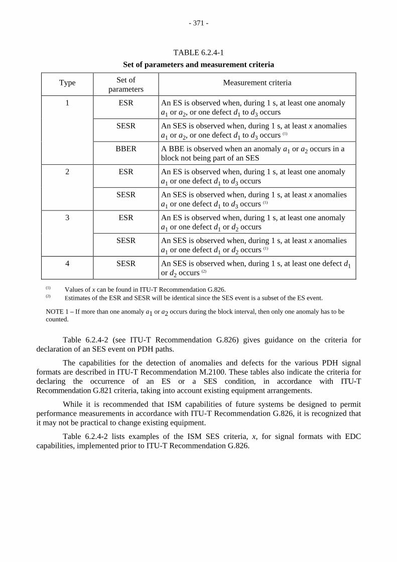
- 371 -

TABLE 6.2.4-1 Set of parameters and measurement criteria

Type Set of parameters

Measurement criteria

1 ESR An ES is observed when, during 1 s, at least one anomaly a1 or a2, or one defect d1 to d3 occurs

SESR An SES is observed when, during 1 s, at least x anomalies a1 or a2, or one defect d1 to d3 occurs (1)

BBER A BBE is observed when an anomaly a1 or a2 occurs in a block not being part of an SES

2 ESR An ES is observed when, during 1 s, at least one anomaly a1 or one defect d1 to d3 occurs

SESR An SES is observed when, during 1 s, at least x anomalies a1 or one defect d1 to d3 occurs (1)

3 ESR An ES is observed when, during 1 s, at least one anomaly a1 or one defect d1 or d2 occurs

SESR An SES is observed when, during 1 s, at least x anomalies a1 or one defect d1 or d2 occurs (1)

4 SESR An SES is observed when, during 1 s, at least one defect d1 or d2 occurs (2)

(1) Values of x can be found in ITU-T Recommendation G.826. (2) Estimates of the ESR and SESR will be identical since the SES event is a subset of the ES event.

NOTE 1 – If more than one anomaly a1 or a2 occurs during the block interval, then only one anomaly has to be counted.

Table 6.2.4-2 (see ITU-T Recommendation G.826) gives guidance on the criteria for declaration of an SES event on PDH paths.

The capabilities for the detection of anomalies and defects for the various PDH signal formats are described in ITU-T Recommendation M.2100. These tables also indicate the criteria for declaring the occurrence of an ES or a SES condition, in accordance with ITU-T Recommendation G.821 criteria, taking into account existing equipment arrangements.

While it is recommended that ISM capabilities of future systems be designed to permit performance measurements in accordance with ITU-T Recommendation G.826, it is recognized that it may not be practical to change existing equipment.

Table 6.2.4-2 lists examples of the ISM SES criteria, x, for signal formats with EDC capabilities, implemented prior to ITU-T Recommendation G.826.

- 372 -

TABLE 6.2.4-2 Criteria for declaration of an SES event on PDH paths

Bit rate (kbit/s) 1 544 2 048 44 736

ITU-T Recommendation G.704 G.704 G.752

EDC type CRC-6 CRC-4 Single bit parity check

Block/s 333 1 000 9 398

Bit/block 4 632 2 048 4 760

SES threshold used on equipment developed prior to the acceptance of ITU-T Rec. G.826

x = 320

x = 805

x = 45 or x = 2 444

as suggested in ITU-T Rec. M.2100

ISM threshold based on ITU-T Rec. G.826 SES (30% errored blocks)

(1)

(1)

x = 2 444 (2)

(1) Due to the fact that there is a large population of systems in service, the criteria for declaration of an SES will not change for the frame formats of these systems.

(2) This figure takes into account the fact that, although 30% of the blocks could contain errors, a smaller value will be detected by the EDC due to the inability of the simple parity code to detect even numbers of errors in a block. It should be noted that such a simple EDC is non-compliant with the intent of ITU-T Recommendation G.826.

The available remote in-service indications such as RDI or, if provided, REI are used at the near end to estimate the number of SES occurring at the far end.

6.2.4.11 ISM of SDH paths

For ISM estimation of SDH-DRRS error performance and availability objectives the special overhead bits could be used (see § 6.1). The specification of an equipment for error performance monitoring on SDH signals is contained in ITU-T Recommendation O.181. In this Recommendation the different measurement modes are defined depending on the structure of the received STM-N signal at the connection point and also on the type of SDH network entities (i.e. multiplex section, regeneration section, path...) crossed by the measured signal.

For each measurement mode, and according to the type of STM-N signal considered, a subset of network events to be monitored is given in § 6.2.5.

In-service anomaly conditions are used to determine the error performance of an SDH path when the path is not in a defect state. The following anomaly is defined:

– a1: an EB as indicated by an EDC.

In-service defect conditions are used in ITU-T Recommendations G.707 and G.783 relevant to SDH equipment to determine the change of performance state which may occur on a path. Tables 6.2.4-3 and 6.2.4-4 show the defects used in ITU-T Recommendation G.826.

- 373 -

TABLE 6.2.4-3

Defects resulting in a near-end severely errored second (SES)

Defect No. Near-end defects Kind of path

d14 LP UNEQ

d13 LP TIM Applicable to

d12 TU LOP lower order paths

d11 TU AIS

d10 HP LOM (1)

d9 HP PLM

d8 HP UNEQ

d7 HP TIM Applicable to

d6 AU LOP higher order paths

d5 AU AIS

(1) This defect is not related to VC-3.

NOTE 1 – VC AIS defect is not included above as it only applies to a segment of a path.

NOTE 2 – The above defects are path defects only. Section defects such as MS AIS, RS TIM, STM LOF and STM LOS give rise to an AIS defect in the path layers.

AIS : Alarm Indication Signal HP : Higher order Path LOM : Loss of Multiframe LOP : Loss of Pointer LP: : Lower order Path TIM : Trace Identifier Mismatch TU : Tributary Unit UNEQ : UnEquipped

TABLE 6.2.4-4

Defects resulting in a far-end severely errored second (SES)

Defect No. Far-end defects Kind of path d16 LP RDI Applicable to

lower order paths d15 HP RDI Applicable to

higher order paths

RDI : Remote Defect Indication

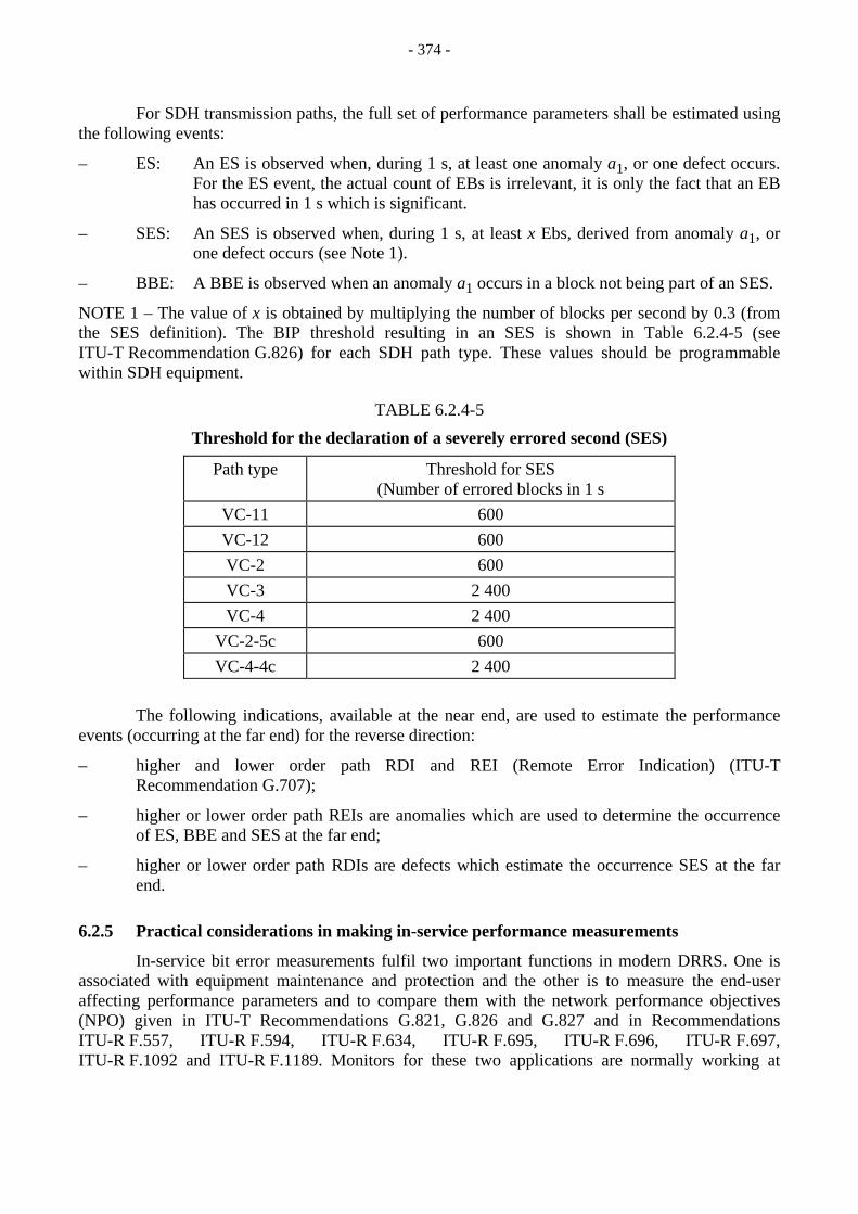
- 374 -

For SDH transmission paths, the full set of performance parameters shall be estimated using the following events:

– ES: An ES is observed when, during 1 s, at least one anomaly a1, or one defect occurs. For the ES event, the actual count of EBs is irrelevant, it is only the fact that an EB has occurred in 1 s which is significant.

– SES: An SES is observed when, during 1 s, at least x Ebs, derived from anomaly a1, or one defect occurs (see Note 1).

– BBE: A BBE is observed when an anomaly a1 occurs in a block not being part of an SES.

NOTE 1 – The value of x is obtained by multiplying the number of blocks per second by 0.3 (from the SES definition). The BIP threshold resulting in an SES is shown in Table 6.2.4-5 (see ITU-T Recommendation G.826) for each SDH path type. These values should be programmable within SDH equipment.

TABLE 6.2.4-5

Threshold for the declaration of a severely errored second (SES)

Path type Threshold for SES (Number of errored blocks in 1 s

VC-11 600 VC-12 600 VC-2 600 VC-3 2 400 VC-4 2 400

VC-2-5c 600 VC-4-4c 2 400

The following indications, available at the near end, are used to estimate the performance events (occurring at the far end) for the reverse direction:

– higher and lower order path RDI and REI (Remote Error Indication) (ITU-T Recommendation G.707);

– higher or lower order path REIs are anomalies which are used to determine the occurrence of ES, BBE and SES at the far end;

– higher or lower order path RDIs are defects which estimate the occurrence SES at the far end.

6.2.5 Practical considerations in making in-service performance measurements

In-service bit error measurements fulfil two important functions in modern DRRS. One is associated with equipment maintenance and protection and the other is to measure the end-user affecting performance parameters and to compare them with the network performance objectives (NPO) given in ITU-T Recommendations G.821, G.826 and G.827 and in Recommendations ITU-R F.557, ITU-R F.594, ITU-R F.634, ITU-R F.695, ITU-R F.696, ITU-R F.697, ITU-R F.1092 and ITU-R F.1189. Monitors for these two applications are normally working at

- 375 -

different bit rates and most importantly, they are located at different points in the digital radio system. It might be advantageous to provide both types of monitors in a DRRS.

These monitors often have some local displays but their outputs will normally be transmitted to the central location of a telecommunications management network. Several monitors in one location will first be reconnected (the Q1 and Q2 interfaces) to a mediation device which, in turn, delivers the maintenance signals over the data communications network (the Q3 interface) to the central management location. Monitors could also be connected to the central location using the Q3 interface.

6.2.5.1 Monitors used for equipment maintenance and protection

The radio system bit rate is normally higher than the hierarchical rate existing at the T-T' interconnection points of digital radio switching sections. This is because within a switch section several hierarchical rate signals may be multiplexed together with special overhead bits that may be used for error monitoring, forward error correction and voice order wires. Using parity bits, errors can be checked at the receiving end of the switch section and, sometimes, at individual radio repeaters. The main reason for this kind of error monitoring is to provide internal radio system maintenance and to initiate automatic protection switching. The monitor in these applications is typically located before error correction has taken place and ahead of the receive-end protection switch. Therefore, the performance seen by the monitor will be considerably worse than seen by the end user. This is very useful for radio system maintenance because degradations are detected before they become noticeable by the end user.

Improvements by error correction (EC) and protection switching can be very substantial. EC, for instance, can reduce the number of errors by many orders of magnitude and protection switching, especially errorless switching, can reduce channel outages caused by fading or equipment failures by another large factor. For this reason error measurements within a switch section are not used for comparison with NPOs. Requirements for these measurements have to be derived from the NPOs, but this can only be done in a very approximate way.

6.2.5.2 Monitors for checking network performance objectives

These monitors are most appropriately bridged on to the receive side interconnect point TT' where they measure the bit errors at the hierarchical rate as seen by the end user. ISMs require the presence of parity bits that are transmitted in the hierarchical frame structure. The DS3 signal (44 736 Mbit/s) of the North American hierarchy has the P-parity bits available, but they are normally reset at the end of each switch section and are therefore not useful at the interconnect points RR'. More recently, so-called C-parity bits have become available in DS3. They are set in the multiplexer at the beginning of the digital path and can be monitored along the path at points TT'.

As indicated earlier, an estimate of error performance can also be obtained by observing special sample pulses that were inserted in the bit stream. In the case of the DS3 signal, F and M framing pulses are being used for this purpose. The use of framing pulses for bit error measurements requires a longer measuring time compared to systems that are parity bits, as mentioned earlier.

After having been estimated by one of these methods, the bit errors are then processed according to the algorithm given in Recommendation ITU-R F.700. This yields errored seconds, severely errored seconds, degraded minutes and unavailable time, and allows direct comparison with the ISDN objectives at the 64 kbit/s basic rate. Monitors connected to the TT' points measure the performance along a digital path beginning with the originating multiplexer. By forming the

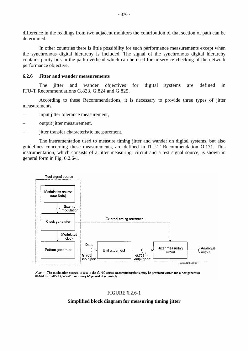
- 376 -

difference in the readings from two adjacent monitors the contribution of that section of path can be determined.

In other countries there is little possibility for such performance measurements except when the synchronous digital hierarchy is included. The signal of the synchronous digital hierarchy contains parity bits in the path overhead which can be used for in-service checking of the network performance objective.

6.2.6 Jitter and wander measurements

The jitter and wander objectives for digital systems are defined in ITU-T Recommendations G.823, G.824 and G.825.

According to these Recommendations, it is necessary to provide three types of jitter measurements:

– input jitter tolerance measurement,

– output jitter measurement,

– jitter transfer characteristic measurement.

The instrumentation used to measure timing jitter and wander on digital systems, but also guidelines concerning these measurements, are defined in ITU-T Recommendation O.171. This instrumentation, which consists of a jitter measuring, circuit and a test signal source, is shown in general form in Fig. 6.2.6-1.

FIGURE 6.2.6-1

Simplified block diagram for measuring timing jitter

- 377 -

6.2.6.1 Input jitter tolerance measurement

Equipment jitter tolerance is specified with jitter tolerance templates. Each template defines the region over which the equipment must operate without suffering the designated degradation of error performance. The difference between the template and actual equipment tolerance curve represents the operating jitter margin, illustrated in Fig. 6.2.6-2.

The sinusoidal jitter amplitudes that an equipment actually tolerated at a given frequency are defined as all amplitudes up to, but not including, that which causes the designated degradation of error performance.

The designated degradation of error performance may be expressed in terms of either BER penalty or onset of error criteria. The existence of two criteria arises because the input jitter tolerance of an individual digital equipment is primarily determined by the following two factors:

– the ability of the input clock recovery circuit to accurately recover clock from a jittered data signal, possibly in the presence of other degradations (pulse distribution, cross-talk, noise, etc.);

– the ability of other components to accommodate dynamically varying input data rates (e.g., pulse justification capacity and synchronizer or desynchronizer buffer size in an asynchronous digital multiplex).

The BER penalty criterion allows environment independent determination of the decision circuit alignment jitter allocation, which is critical for evaluating the first factor.

FIGURE 6.2.6-2

Actual tolerance measurement and tolerance template relationship

- 378 -

6.2.6.2 Output jitter measurement

Output jitter measurement falls within two categories:

– network output jitter at hierarchical interfaces,

– intrinsic jitter generated by individual digital equipment.

Measurement of output jitter may be in terms of r.m.s and peak-to-peak amplitudes over designated frequency ranges, and may require statistical characterization.

Output jitter measurements utilise either live traffic or controlled data patterns.

Output jitter measurements at network hierarchical interfaces typically use a live traffic signal. This technique involves demodulating the jitter from the live traffic at the output of a network interface, selectively filtering the jitter, and measuring the true r.m.s or true peak-to-peak amplitude of the jitter over the specified measurement time interval.

Measurement of intrinsic jitter in individual digital equipment requires the application of controlled data patterns. Controlled data patterns are generally applicable in laboratory, factory and out-of-service situation.

Where it is desirable to obtain more detailed information regarding output jitter power (specifically, jitter generated in digital regenerators), jitter may be further categorized in terms of random and systematic components. The primary reasons for distinguishing between random and systematic jitter are to enable the comparison of measurement results with theoretical computation, and to refine equipment design.

6.2.6.3 Jitter transfer characteristics

The jitter transfer characteristic of an individual digital equipment is defined as the ratio of the output jitter to the applied input jitter as a function of frequency. If the relationship between the jitter appearing at the input and output ports of digital equipment can be described in terms of a linear process (a process which is both additive and homogeneous), the term “jitter transfer function” is used. The relationship between jitter appearing at the input and output ports of some types of digital equipment cannot be described in terms of a “jitter transfer function”. In such cases, different measurement techniques may be necessary to obtain meaningful results.

Jitter transfer measurements are commonly required for clock recovery circuits and desynchronizer phase smoothing circuits. Measurement of the jitter transfer function of a linear clock recovery circuit is generally straightforward. However, measurement of the jitter transfer function of a linear desynchronizer phase smoothing circuit requires specialised techniques because it is embedded in a non-linear asynchronous digital multiplex.

For more details concerning jitter measurements see ITU-T Recommendation O.171.

6.2.6.4 Wander measurements

Because of the low frequency of the phase variations to be evaluated, wander is a quantity which requires a special test configuration. When performing jitter measurements, the required reference timing signal is normally produced locally. By means of a phase-locked loop it is derived

- 379 -

from the average phase of the signal to be measured. Such a phase-locked loop cannot be realized to cope with the requirements of wander measurements.

Therefore, wander measurements always require an external reference signal of adequate stability.

ITU-T Recommendation O.171 contains information on test configurations for wander measurements which are in accordance with ITU-T Recommendation G.810.

If the stability of a clock is to be measured, the measurement set-up is similar to that described above.

The following wander quantities should be measured:

– time deviation,

– maximum time interval error,

– Allan deviation.

Especially for the measurement of wander, an input for an external reference signal is required. This input shall accept clock signals of the bit rate of 1 544 kbit/s or 2 048 kbit/s and sinusoidal signals at 1 544 kHz or 2 048 kHz as a reference.

6.2.7 Digital radio-relay equipment measurement

The International Electrotechnical Commission (IEC) is currently adopting standards for measurements of digital radio systems. The use of these standards will enable easy comparison of different equipment and manufacturers of test equipment will be able to provide standard test equipment for compatible measurement solutions.

It may be useful to note that certain characteristics of digital radio-relay equipment are specific (such as signature, constellation, XPIC improvement factor, interference sensitivity etc).

More detailed information about the measurement of equipment signature and XPIC is given below as examples. For further information see IEC, SC 12E, Publication 835.

6.2.7.1 Equipment signature

Signatures can be measured by approximating actual fades by two-ray simulator in the laboratory and determining the model parameters that cause, for example, an error ratio of 10-3. The simplified three-ray model has the transfer function:

H(ω) = α [1 − b exp(-j(ω - ω0 )τ)] (6.2.7-1)

where a unity amplitude direct ray, and a ray of amplitude “b” delayed by τ, is assumed, and “α” is a scaling factor. The “notch” point of this fade is f0

away from the channel centre frequency, and has a depth B = − 20 log λ (λ = 1 − b).

- 380 -

FIGURE 6.2.7-1

Basic arrangement for the measurement of signatures

The signature is then a plot of critical value B, as a function of f0 at the outage error ratio. The most often used value for τ is 6.3 ns but sometimes signatures are measured for other values of τ. The signature width remains practically constant versus delay, except for the case when delay approaches to zero, when it doubles for halving delay.

Critical amplitude bc (τ) = 1 – 10(-Bc /20) decreases from bc (0) = 1 to a non-zero value bi

for a very large delay. Different rules for bc (τ) have been proposed. The linear one, applicable for small delays only, says that the height (λ) is proportional to τ.

A fading simulator may be implemented at IF or RF. A typical IF two-ray simulator is shown in Fig. 6.2-7-1. An example of measured signature is shown in Fig. 6.2.7-2.

FIGURE 6.2.7-2

Example of a signature MP : Minimum Phase NMP : Non-Minimum Phase

- 381 -

6.2.7.2 Cross-polarization interference cancellers

This section deals with measurement for “cross-polarization interference cancellers” (XPIC) used in digital microwave radio-relay systems.

a) C/N versus cross-polarization isolation

Cross-Polarization Isolation (XPI) as defined for two radio waves transmitted with the same power and orthogonal polarizations, is the ratio at the reception point of the power received from one of the powers from the other wave, in the expected polarization of the first wave.

The set-up for the measurement is shown in Fig. 6.2.7-3. The two modulators are driven by different pseudo random binary signals with each other. After the H- and V-polarization signals are divided into main (cross-polarization main signal) and leaky (cross-polarization interference) paths, the four path-lengths are adjusted at the inputs of the receivers to have the same static path length. Adjustable noise (n) and adjustable cross-polarization interference (i) are added to the two main signals.

FIGURE 6.2.7-3

Set-up for C/N versus XPI measurement

- 382 -

C/N and XPI should be set for both cross-polarized main signal at the demodulator input as follows (two bandpass filters which pass the main signals without noticeable degradation may be needed to measure the noise power):

– noise and cross-polarization interference are switched off, then the main signal power, s, is measured at the output port of the combiner through the calibrated bandpass filter;

– cross-polarization interference and the main signal are switched off, and the noise power, n, is measured at the above-mentioned port;

– the main signal and noise are switched off, and the cross-polarization interference, i, is measured at the above-mentioned port;

– C/N and XPI are defined as follows: C/N = s/n + 10 log (BCAL/B) dB (6.2.7-2) XPI = s/i,

where:

BCAL : equivalent noise bandwidth of the bandpass filter,

B : equivalent noise bandwidth of the main signal receiver.

Cross-polarization interference levels, i, necessary for obtaining the specified BER (e.g. 10-4) are measured by increasing interference levels from the small value, for several noise levels, n, (the ordinary performance). Vary the phase of the phase shifter and determine C/N as indicated above in order to find the worst case value. When noise and/or interference are added to both paths, C/N and XPI should have the same values for both paths, for simplicity.

The “improvement factor” is the XPI difference between the performance with and without the XPIC at the specified C/N and BER.

The measurement of the “improvement factor” requires the XPIC to be disabled. If this is not possible, only the performance with the XPIC is measured. The lock-in performance is measured by decreasing the value of the cross-polarization interference, i, from a lock-out state (high value of interference) of the equipment in the same way as the above-mentioned ordinary measurement.

The above measurements should be carried out for either polarization signal or both polarization signals, if required.

b) XPI (or improvement factor) versus delay difference

The performance of the XPICs is generally sensitive to the delay difference between the cross-polarization interference path and the cross-polarization main signal path.

The set-up for the measurement is shown in Fig. 6.2.7-4. This set-up is the same as the one for C/N versus XPI measurement in Fig. 6.2.7-3 except that a variable delay line (DV) is inserted into the cross-polarization main signal path, e.g. V-polarization. Accordingly, the delay difference between the cross-polarization main signal path can be changed by adjusting DV, and XPI or “improvement factor” at the specified BER (e.g. 10-4 and at the specified C/N) is measured versus the delay difference. Calibration methods of C/N and XPI are the same as above.

- 383 -

The above measurement should be repeated for H-polarization signal inserting DH instead of DV , or for the H- and V-polarization signals inserting both DV and DH, if required.

FIGURE 6.2.7-4

Set-up for XPI versus delay difference measurement

c) XPI (or improvement factor) versus notch depth with dispersive signal

In the above sub-clauses, a non-dispersive cross-polarization interference is used to evaluate XPIC performance. To evaluate the XPIC performance during multipath propagation, a dispersive cross-polarization main signal and a non-dispersive cross-polarization interference should be used.

XPI or “improvement factor” degrades as the notch depth increases, because the equalized waveform distortion of the main signal increases. The XPI or “improvement factor” strongly depends on the adaptive equalizers within the demodulators in the main signal paths.

The measurement set-up is shown in Fig. 6.2.7-5. This arrangement is similar to that for C/N versus XPI measurement in Fig. 6.2.7-3, except that Fading Simulators (FS) are inserted into the main signal paths. The dispersive frequency characteristics are generated by the two-path propagation model. Fading simulators are inserted into the indicated paths and notch frequency, Fn, and two-ray delay difference, τ, are set at the specified values. The measurement should be carried out at the specified C/N and at the specified notch depth, B, by slowly decreasing the XPI from a large value until the BER reaches the specified value (e.g. 10-4). The corresponding XPI value should be noted. The measurement should be repeated for several constant notch depths. There are many sets of the fading characteristics. For simplicity, the two fading simulators should be set to the same notch depth and the same notch frequency.

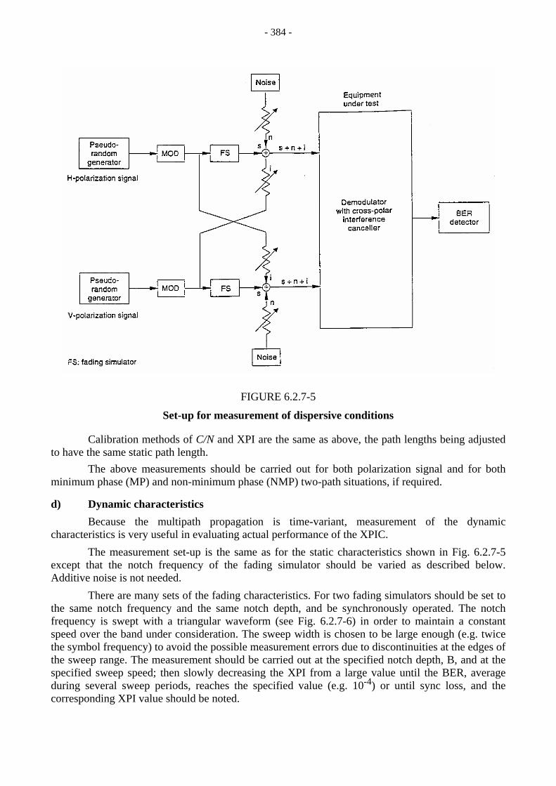
- 384 -

FIGURE 6.2.7-5

Set-up for measurement of dispersive conditions

Calibration methods of C/N and XPI are the same as above, the path lengths being adjusted to have the same static path length. The above measurements should be carried out for both polarization signal and for both minimum phase (MP) and non-minimum phase (NMP) two-path situations, if required.

d) Dynamic characteristics

Because the multipath propagation is time-variant, measurement of the dynamic characteristics is very useful in evaluating actual performance of the XPIC.

The measurement set-up is the same as for the static characteristics shown in Fig. 6.2.7-5 except that the notch frequency of the fading simulator should be varied as described below. Additive noise is not needed.

There are many sets of the fading characteristics. For two fading simulators should be set to the same notch frequency and the same notch depth, and be synchronously operated. The notch frequency is swept with a triangular waveform (see Fig. 6.2.7-6) in order to maintain a constant speed over the band under consideration. The sweep width is chosen to be large enough (e.g. twice the symbol frequency) to avoid the possible measurement errors due to discontinuities at the edges of the sweep range. The measurement should be carried out at the specified notch depth, B, and at the specified sweep speed; then slowly decreasing the XPI from a large value until the BER, average during several sweep periods, reaches the specified value (e.g. 10-4) or until sync loss, and the corresponding XPI value should be noted.

- 385 -

The measurement should be repeated for several sweep speeds. The measurement should be carried out for both minimum phase (MP) and non-minimum phase (NMP) two-path situations, if required.

FIGURE 6.2.7-6

Illustration of sweep waveform for measurement of dynamic characteristics

- 386 -


International Electrotechnical Commission (IEC) SC12E. Publication 835, Part 2, Methods of measurement for equipment used in digital microwave transmission systems.

ITU-R Documents

[1996]: a. 9A/31, 73-78. ITU-R Report on performance limits to be respected for bringing-into-service and maintenance of digital radio relay systems; b. 9A/31, 58-63. ITU-R Preliminary draft new Recommendation. Performance limits for bringing-into-service of digital radio-relay systems operating in PDH and SDH based international paths and sections.

BIBLIOGRAPHY


Rec. ITU-R F.557 Availability objectives for radio-relay systems over a hypothetical reference circuit and a hypothetical reference digital path.



Rec. ITU-R F.695 Availability objectives for real digital radio-relay links forming part of a high-grade circuit within an integrated services digital network.


Rec. ITU-R F.697 Error performance and availability objectives for the local-grade portion at each end of an ISDN connection utilizing digital radio-relay systems.

Rec. ITU-R F.700 Error performance and availability measurement algorithm for digital radio-relay links at the system bit-rate interface.


Rec. ITU-R F.751 Transmission characteristics and performance requirements of radio-relay systems for SDH-based networks.

Rec. ITU-R F. 1094 Maximum allowable error performance and availability degradations to digital radio-relay systems arising from interference from emissions and radiations from other sources.

- 387 -


ITU-T Rec. G.704 Synchronous frame structures used at 1 544, 6 312, 2 408, 8 488 and 44 736 kbit/s hierarchical levels.

ITU-T Rec. G.773 Protocol suits for Q-interferences for management of transmission systems.

ITU-T Rec. G.775 Loss of signal (LOS) and alarm indication signal (AIS) defect detection and clearance criteria.

ITU-T Rec. G.821 Error performance of an international digital connection operating at a bit rate below the primary rate and forming part of an integrated services digital network.

ITU-T Rec. G.823 The control of jitter and wander within digital networks which are based on the 2 048 kbit/s hierarchy.

ITU-T Rec. G.824 The control of jitter and wander within digital networks which are based on the 1 544 kbit/s hierarchy.

ITU-T Rec. G.825 The control of jitter and wander within digital networks which are based on the synchronous digital hierarchy (SDH).

ITU-T Rec. G.826 Error performances parameters and objectives for international, constant bit rate digital paths at or above the primary rate.

ITU-T Rec. M.20 Maintenance philosophy for telecommunication networks.

ITU-T Rec. M.34 Performance monitoring on international transmission systems and equipment.

ITU-T Rec. M.2100 Performance limits for bringing-into-service and maintenance of international PDH paths, sections and transmission systems.

ITU-T Rec. M.2101 Performance limits for bringing-into-service and maintenance of international SDH paths and multiplex sections.

ITU-T Rec. M.2110 Bringing-into-service international digital path, sections and transmission systems.

ITU-T Rec. M.2120 Digital path, section and transmission system fault detection and localization procedures.

ITU-T Rec. M.3000 Overview of TMN Recommendations.

ITU-T Rec. O.150 Digital test patterns for performance measurements on digital transmission equipment.

ITU-T Rec. O.151 Error performance measuring equipment operating at the primary rate and above.

ITU-T Rec. O.152 Error performance measuring equipment for bit rates of 64 kbit/s and N x 64 kbit/s.

ITU-T Rec. O.153 Basic parameters for measurements of error performance at bit rates below the primary rate.

ITU-T Rec. O.161 In-service code violation monitors for digital systems.

- 388 -

ITU-T Rec. O.162 Equipment to perform in-service monitoring on 2 048, 8 448, 34 368 and 139 264 kbit/s signals.

ITU-T Rec. O.163 Equipment to perform in-service monitoring on 1 544 kbit/s signals.

ITU-T Rec. O.171 Timing jitter measuring equipment for digital systems.

ITU-T Rec. O.181 Equipment to assess error performance on STM-N SDH interfaces.

ITU-T Rec. V.41 Code independent error control system.

- 389 -

LIST OF ABBREVIATIONS

A/D Analogue-to-Digital

AASE Adaptive Amplitude Slope Equalizer

ACI Adjacent-Channel Interference

ADL Adaptive Digital Linearizer

AEQ Adaptive Amplitude Equalisation

AGC Automatic Gain Control

AIS Alarm Indication Signal

AMPS Advanced Mobile Phone Service

APO Allocated Performance Objective

AR Availability Ratio

ARDIS Advanced Radio Data Information Service

ASK Amplitude Shift Keying

ATM Asynchronous Transfer Mode

ATPC Adaptive Transmitter Power Control

ATT Adjustable Attenuator

AU Administrative Unit

AUG Administrative Unit Group

AWGN Additive White Gaussian Noise

AXPIC Adaptive Cross Polar Interference Canceller

AZD Ambiguity Zone Detection

BB Baseband

BBC Baseband Bit Combining

BBE Background Block Error

BBER Background Block Error Ratio

BCH Bose-Chaudhuri-Hocquenghem codes

BCM Block Coded Modulation

BER Bit Error Ratio

BERTS Bit Error Ratio Test Sets

BF Bandwidth correction Factor

BIP Bit Interleaved Parity

- 390 -

BIS Bringing-Into-Service

BPF Bandpass Filters

BSC Base Station Controllers

BSS Broadcasting-Satellite Service

BTF Binary Transversal Filter

BTS Base Transceiver Stations

C-n Container-n

CCI Co-Channel Interference

CEPT European Conference of Postal and Telecommunication Administrations

COMB In-Phase Power Combining

COMB + AEQ Adaptive Amplitude Equalisation With Power Combining

CPA Co-Polar Attenuation

CPFSK Continuous Phase FSK

CPM Continuous Phase Modulation

CRC Cyclic Redundancy Code

DADT Different Absolute Delay Time

DAV Digits Above Voice

DCS Digital Cellular System

DEC Decision Circuit

DEC FB Decision Feedback circuit

DEMOD No Fading Countermeasures

DFE Decision Feedback Equalizer

DIV Digits In Voice

DM Degraded Minute

DMA Deferred Maintenance Alarm

DMR Digital Microwave Radio

DR Dispersion Ratio

DRO Dielectric Resonator Oscillator

DRRS Digital Radio-Relay Systems

DTE Digital Transversal Equalizer

DUV Digits Under Voice

e.i.r.p. Equivalent isotropically radiated power

- 391 -

EB Errored Block

EC Error Correction

EDC Error Detection Code

EDO Equipment Design Objective

EOW Engineering Order Wire

EQ Slope Equalizer

EQPM SW Equipment Switch

ES Errored Second

ESR Errored Second Ratio

ETSI European Telecommunication Standards Institute

EUT Entity Under Test

FAS Frame Alignment Signal

FAT Field Acceptance Tests

FAW Frame Alignment Word

FCC Federal Communication Commission (United States of America)

FEC Forward Error Correction

FDM Frequency Division Multiplexing

FDP Fractional Degradation in Performance

FEC Forward Error Correction

FET Field Effect Transistor

FM Frequency Modulation

FRP Fibre Reinforced Plastic

FS Fixed Service

fs Frontier station

FSE Fractionally-Spaced Equalizers

FSF Frequency Selective Fading

FSK Frequency Shift Keying

FSL Free Space Loss

FSS Fixed-Satellite Service

FZ Fresnel Zones

GaAs Gallium Arsenide

GD Group Delay

- 392 -

GPS Global Positioning System

GSM Global System for Mobile communications

GSO Geostationary-Satellite Orbit

HDRP Hypothetical Digital Reference Path

HDTV High Definition TV

HL SW Hitless Switch

HOVC Higher Order Virtual Container Layer

HP Higher Order Path

HRDL Hypothetical Reference Digital Link

HRDP Hypothetical Reference Digital Path

HRDS Hypothetical Reference Digital Section

HRP Hypothetical Reference Path

HRX Hypothetical Reference Connection

IBAD In-Band Amplitude Dispersion

IBPD In-Band Power-Difference

ICPCE Inter-Country Path Core Element

IEC International Electrotechnical Commission

IF Intermediate Frequency

IG International Gateway

IP Intermodulation Products

IPCE International Path Core Element

IRF Interference Reduction Factor

IRFXPIC Interference Reduction Factor of XPIC

ISDN Integrated Services Digital Network

ISI Inter-Symbol Interference

ISM In-Service Measurement

ITU International Telecommunication Union

ITU-R Radiocommunication Sector of the ITU

ITU-T Telecommunication Standardization Sector of the ITU

LAD Linear Amplitude Dispersion

LAN Local Area Networks

LE Local Exchange

- 393 -

LEC Lee Error Correction codes

LEO Low-Earth-Orbits

LMS Least Mean Square

LNA Low Noise Amplifier

LO Local Oscillator

LOF Loss Of Frame

LOM Loss Of Multiframe

LOP Loss of Pointer

LOS Line-of-Sight

LOVC Lower Order Virtual Container layer

LP Lower Order Path

LSB Lower Side Band

LSS Loss of Sequence Synchronisation

MAN Metropolitan Area Network

MAP Maximum Power

ME Maintenance Entity

MED DEV Mediation Device

MEF Maintenance Entity Function

MEI Maintenance Event Information

MID Minimum Dispersion Combiner

MID-SD Minimum In-Band Amplitude Dispersion Space Diversity

MLCM Multi-Level Coded Modulation

MLE Maximum Level Error

MLSE Maximum Likelihood Sequence Estimation

MMSE Minimum Mean Square Error

MO Mean time between digital path Outages

MP Minimum Phase

MS Multiplexer Section layer

MSC Mobile Switching Centres

MSE Mean-Square Error

MSOH Multiplex Section Overhead

MTBF Mean Time Between Failure

- 394 -

MTF Multipath Transfer Function

MTTR Mean Time To Repair

NE Network Element

NFD Net Filter Discrimination

NMP Non-Minimum Phase

NNI Network Node Interface

NPO Network Performance Objective

NRZ Non Return to Zero

NSMA United States National Spectrum Managers Association

NYQ Nyquist Filter

OBO Output Back-Off

OI Outage Intensity

OMT Orthomode Transducer

OOF Out Of Frame

OOS Out-Of-Service

OS Operation System

OSI Open System Interconnection

OSM Out-of-Service Measurement

PAM Pulse-Amplitude Modulation

PC Primary Centre

PCE Path Core Element

PCM Pulse Code Modulation

PCN Personal Communications Networks

PDF Probability Density Function

PDH Plesiochronous Digital Hierarchy

PEP Path End-Point

PFD Power Flux-Density

PLBIS Performance Limits for Bringing-Into-Service

PMA Prompt Maintenance Alarm

PMPL Post Maintenance Performance Limits

PO Performance Objectives

PRBS Pseudo-Random Binary Sequence

- 395 -

PROT SW CONT Protection Switch Control

PRS Partial Response Signals

PRV Partial Response Violation

PSK Phase Shift Keying

PTR Pointer

QAM Quadrature Amplitude Modulation

QASK Quadrature ASK

QPR Quadrature Partial Response modulation

QPRS Quadrature PRS

RBER Residual Bit Error Ratio

RDI Remote Defect Indication

REI Remote Error Indication

rf Routing factor

RF Radio Frequency

RFCOH Radio Frame Complementary Over-Head

RLAN Radio Local Area Networks

r.m.s Root mean square

RPO Reference Performance Objectives

RR-RP Radio-Relay Reference Point

RRCs ITU Regional Radiocommunication Conferences

RS Reed-Solomon codes

RSOH Regenerator Section Overhead

SC Secondary Centre

SCR Scrambler

SDH Synchronous Digital Hierarchy

SEF Support Entity Function

SER Symbol Error Ratio

SES Severely Errored Second

SESR Severely Errored Second Ratio

SFF Single Frequency Fade

SG System Gain

SMF System Multiplexing Filter

- 396 -

SNR Signal-to-Noise Ratio

SOH Section Overhead

SONET Synchronous Optical Network

STM-1 Synchronous Transport Module - Level 1 (155.52 Mbit/s)

STS-1 Sub-STM-1 Signal Format (51.84 Mbit/s = STM-1:3)

SVC Service Channel

TC Tertiary Centre

TCM Trellis Coded Modulation

TDM Time Division Multiplexing

TE Transversal Equalizer

TIM Trace Identifier Mismatch

TMN Telecommunications Management Network

TMNS Transmission Management Network Services

TSE Test Sequence Error

TSS Test Signal Structures

TU Tributary Unit

TWT Travelling Wave Tube

UFI Upstream Failure Indication

UI Unit Intervals

UNEQ UnEquipped

UR Unavailability Ratio

USB Upper Side Band

VC Virtual Containers

VCO Voltage Controlled Oscillator

VMR Violation Monitor Restorer

VSWR Voltage Standing Wave Ratio

WRCs ITU World Radiocommunication Conferences

XPD Cross-Polarization Discrimination

XPI Cross-Polarization Isolation

XPIC Cross-Polarization Interference Canceller

ZF Zero-Forcing (algorithm)

HANDBOOK – DIGITAL RADIO-RELAY SYSTEMS · 2018-05-25 · - 1 - CHAPTER 1 INTRODUCTION 1.1 Intent...

Documents

Transcript of HANDBOOK – DIGITAL RADIO-RELAY SYSTEMS · 2018-05-25 · - 1 - CHAPTER 1 INTRODUCTION 1.1 Intent...