Reconciling forecasts of infant mortality rates at national and

sub-national levels: Grouped time-series methods

Han Lin Shang 1

Australian National University

Abstract

Mortality rates are often disaggregated by different attributes, such as sex, state,

education, religion or ethnicity. Forecasting mortality rates at the national and sub-

national levels plays an important role in making social policies associated with the

national and sub-national levels. However, base forecasts at the sub-national levels may

not add up to the forecasts at the national level. To address this issue, we consider

the problem of reconciling mortality rate forecasts from the viewpoint of grouped

time-series forecasting methods (Hyndman, Ahmed, Athanasopoulos and Shang, 2011).

A bottom-up method and an optimal combination method are applied to produce point

forecasts of infant mortality rates that are aggregated appropriately across the different

levels of a hierarchy. We extend these two methods by considering the reconciliation of

interval forecasts through a bootstrap procedure. Using the regional infant mortality

rates in Australia, we investigate the one-step-ahead to 20-step-ahead point and interval

forecast accuracies among the independent and these two grouped time-series forecasting

methods. The proposed methods are shown to be useful for reconciling point and

interval forecasts of demographic rates at the national and sub-national levels, and

would be beneficial for government policy decisions regarding the allocations of current

and future resources at both the national and sub-national levels.

Keywords bottom-up forecasts – hierarchical forecasting – optimal combination – reconciling

forecasts – Australian infant mortality rates

1Postal address: Research School of Finance, Actuarial Studies and Statistics, Australian NationalUniversity, Acton ACT 2601, Australia; Telephone number: +61(2) 6125 0535; Fax number: +61(2) 61250087; Email address: hanlin.shang@anu.edu.au

1

arX

iv:1

608.

0871

8v1

[st

at.A

P] 3

1 A

ug 2

016

1 Introduction

The infant mortality rate is a useful indicator of a country’s level of health or development

and it is a component of the physical quality of life index. In some societies, sex-specific

infant mortality may reveal gender inequalities. For instance, many Asian countries are

known to have a preference for sons, which has stimulated research into gender bias, such

as in India (Griffiths, Matthews and Hinde, 2000), Bangladesh (Rahman and DaVanzo,

1993), China (Coale and Banister, 1996), the Republic of Korea (Park and Cho, 1995), and

sub-Saharan Africa (Flatøand Kotsadam, 2014). Anomalous female infant mortality is a sign

of gender stratification, and as such is in need of detailed investigation by social and medical

scientists.

As a part of the United Nations Millennium Development Goals, the infant mortality rate

has been widely studied by official statistical agencies worldwide, including the United Nations

Statistics Division (http://unstats.un.org/unsd/demographic/products/vitstats), the

United Nations International Children’s Emergency Fund (http://www.unicef.org), the

World Health Organization (http://www.who.int/whosis/mort/en), the World Bank (data

.worldbank.org/indicator/SP.DYN.IMRT.IN), as well as demographic and medical re-

search communities. For example, Fuse and Crenshaw (2006) investigated the gender

imbalance in infant mortality in a cross-national study consisting of many developing nations,

while Drevenstedt, Crimmins, Vasunilashorn and Finch (2008) studied the rise and fall of

excess male infant mortality in a cross-national study consisting of many developed nations.

Furthermore, Abdel-Latif, Bajuk, Oei, Vincent, Sutton and Lui (2006) studied the differences

in infant mortality between rural and urban areas in Australia.

It is not only important to analyze infant mortality by state and examine variations

across different states, but also important to analyze the infant mortality rate by sex and

examine the hypothesis whether or not the female infant mortality rate will continue to

be higher than the male infant mortality rate. With both aggregated and disaggregated

historical time series, we aim to model and forecast sex-specific infant mortality rates at

national and sub-national levels. When these data are forecast independently without any

constraint, we often confront the account balancing problem, where the forecasts at the

2

sub-national level may not add up to the forecasts at the national level. This is known as

forecast reconciliation, which has long been studied by Stone, Champernowne and Meade

(1942) and further studied by Weale (1988) and Sefton and Weale (2009), in the context of

balancing the national economic account. Here, we extend this forecast reconciliation from

economics to demography.

The reconciliation methods proposed will not only enhance interpretation of mortality

forecasts, but can also improve forecast accuracy as it obeys a group structure. Any

improvements in the forecast accuracy of mortality would be beneficial for governments, in

particular for determining age of retirements; annuity providers and corporate pension funds

for allocating pension benefits at the national and sub-national levels.

To the best of our knowledge, there is little or no work on reconciling forecasts of

infant mortality rates at the different levels of a hierarchy, where infant mortality rates

can be disaggregated by sex and state. We consider a bottom-up method and an optimal

combination method of Hyndman et al. (2011), and extend these methods to model rates

instead of counts. These methods do not only produce point forecasts for infant mortality

rates at the national and sub-national levels, but also the point forecasts at the sub-national

level sum up to the forecasts at the national level. As a result, the point forecasts and the

original time series both preserve the group structure. The main contribution of this paper is

to put forward a bootstrap procedure for constructing prediction intervals for the bottom-up

and optimal combination methods, since forecast uncertainty can never be overlooked.

When we observe multiple time series that are correlated, we often confront the so-called

grouped time series. Grouped time series are typically time series organized in a hierarchical

structure based on different attributes, such as sex, state, education, religion or ethnicity.

For example, Athanasopoulos, Ahmed and Hyndman (2009) disaggregate the Australian

tourism demand by states. Tourism demand within each state is then disaggregated into

different zones. Tourism demand within each zone is further divided into different regions.

In demographic forecasting, the infant mortality rates in Australia can first be disaggregated

by sex. Within each sex, mortality rates can then be further disaggregated by the different

Australian states. The first example is referred to as a hierarchical time series, in which

3

the order of disaggregation is unique. The second example, which will be studied here, is

called a grouped time series. Grouped time series can be thought of as hierarchical time

series without a unique hierarchical structure. In other words, the infant mortality rates in

Australia can also be first disaggregated by state and then by sex.

Existing approaches to hierarchical/grouped time-series forecasting in econometrics and

statistics usually consider a top-down method, bottom-up method, middle-out method or an

optimal combination method. A top-down method predicts the aggregated series at the top

level and then disaggregates the forecasts based on historical or forecast proportions (see for

example, Gross and Sohl, 1990). The bottom-up method involves forecasting each of the

disaggregated series at the lowest level of the hierarchy and then using simple aggregation

to obtain forecasts at the higher levels of the hierarchy (see for example, Kahn, 1998). In

practice, it is common to combine both methods, where forecasts are obtained for each series

at an intermediate level of the hierarchy, before aggregating them to the series at the top

level and disaggregating them to the series at the bottom level. This method is referred

to as the middle-out method. Hyndman et al. (2011) and Hyndman, Lee and Wang (2016)

proposed an optimal combination method, where base forecasts are obtained independently

for all series at all levels of the hierarchy and then a linear regression model is used with an

ordinary least squares (OLS) or a generalized least squares (GLS) estimator to optimally

combine and reconcile these forecasts. They showed that the revised forecasts do not only

add up across the hierarchy, but they are also unbiased and have minimum variance amongst

all combined forecasts under some simple assumptions (Hyndman et al., 2011).

To the best of our knowledge, these four hierarchical time-series methods are only

applicable to counts not rates. Among the four hierarchical time-series forecasting methods,

the top-down and middle-out methods are not suitable for analyzing grouped time series

because of the non-unique structure of the hierarchy. In Section 2, we first revisit a bottom-up

and an optimal combination method to produce point forecasts of infant mortality rates, and

then propose a bootstrap method to reconcile interval forecasts. Using the Australian infant

mortality rates described in Section 3, we investigate the one-step-ahead to 20-step-ahead

point and interval forecast accuracies in Sections 4 and 5, respectively. Conclusions are given

4

in Section 6, along with some reflections on how the methods developed here might be further

extended. In the Appendix, we present some details on maximum entropy bootstrapping.

2 Some grouped time-series forecasting methods

2.1 Notation

For ease of explanation, we will introduce the notation using the Australian data example

(see Section 3.1 for more details). The generalization to other contexts should be apparent.

The Australian data follow a multilevel geographical hierarchy coupled with a sex grouping

variable. The geographical hierarchy is shown in Fig. 1, where Australia is split into eight

regions.

[Figure 1 about here.]

Let Ct =[Ct,C

>1,t, . . . ,C

>K,t

]>, where Ct is the total of all series at time t = 1, 2, . . . , n,

Ck,t represents the vector of all observations at level k at time t and > symbolizes the matrix

transpose. As shown in Fig. 1, counts at higher levels can be obtained by summing the series

below.

Ct = CR1,t + CR2,t + · · ·+ CR8,t,

CR1,t = CR1∗F,t + CR1∗M,t.

Alternatively, we can also express the hierarchy using a matrix notation (see Athanasopoulos

et al., 2009). Note that

Ct = S ×CK,t,

where S is a “summing” matrix of order m×mK , m represents the total number of series

(1 + 2 + 8 + 16 = 27 for the hierarchy in Fig. 1) and mK represents the total number of

bottom-level series. The summing matrix S, which delineates how the bottom-level series

are aggregated, is consistent with the group structure. For modeling mortality counts, we

5

can express the hierarchy in Fig. 1 as

CT,t

CF,t

CM,t

CR1*T,t

CR2*T,t

...

CR8*T,t

CR1*F,t

CR1*M,t

CR2*F,t

CR2*M,t

...

CR8*F,t

CR8*M,t

︸ ︷︷ ︸

Ct

=

1 1 1 1 1 1 · · · 1 1

1 0 1 0 1 0 · · · 1 0

0 1 0 1 0 1 · · · 0 1

1 1 0 0 0 0 · · · 0 0

0 0 1 1 0 0 · · · 0 0

......

......

...... · · ·

......

0 0 0 0 0 0 · · · 1 1

1 0 0 0 0 0 · · · 0 0

0 1 0 0 0 0 · · · 0 0

0 0 1 0 0 0 · · · 0 0

0 0 0 1 0 0 · · · 0 0

......

......

...... · · ·

......

0 0 0 0 0 0 · · · 1 0

0 0 0 0 0 0 · · · 0 1

︸ ︷︷ ︸

St

CR1*F,t

CR1*M,t

CR2*F,t

CR2*M,t

...

CR8*F,t

CR8*M,t

︸ ︷︷ ︸

CK,t

.

For modeling mortality rates, we can express the hierarchy in Fig. 1 as

RT,t

RF,t

RM,t

RR1*T,t

RR2*T,t

...

RR8*T,t

RR1*F,t

RR1*M,t

RR2*F,t

RR2*M,t

...

RR8*F,t

RR8*M,t

︸ ︷︷ ︸

Rt

=

ER1*F,t

ET,t

ER1*M,t

ET,t

ER2*F,t

ET,t

ER2*M,t

ET,t

ER3*F,t

ET,t

ER3*M,t

ET,t· · · ER8*F,t

ET,t

ER8*M,t

ET,t

ER1*F,t

EF,t0

ER2*F,t

EF,t0

ER3*F,t

EF,t0 · · · ER8*F,t

EF,t0

0ER1*M,t

EM,t0

ER2*M,t

EM,t0

ER3*M,t

EM,t· · · 0

ER8*M,t

EM,t

ER1*F,t

ER1*T,t

ER1*M,t

ER1*T,t0 0 0 0 · · · 0 0

0 0ER2*F,t

ER2*T,t

ER2*M,t

ER2*T,t0 0 · · · 0 0

......

......

...... · · ·

......

0 0 0 0 0 0 · · · ER8*F,t

ER8*T,t

ER8*M,t

ER8*T,t

1 0 0 0 0 0 · · · 0 0

0 1 0 0 0 0 · · · 0 0

0 0 1 0 0 0 · · · 0 0

0 0 0 1 0 0 · · · 0 0

......

......

...... · · ·

......

0 0 0 0 0 0 · · · 1 0

0 0 0 0 0 0 · · · 0 1

︸ ︷︷ ︸

St

RR1*F,t

RR1*M,t

RR2*F,t

RR2*M,t

...

RR8*F,t

RR8*M,t

︸ ︷︷ ︸

RK,t

,

6

where ER1∗F,t/ET,t represents the ratio between the exposure-to-risk for female series in

Region 1 and the exposure-to-risk for total series in entire Australia at time t, and RR1∗F,t =

DR1∗F,t/ER1∗F,t represents the mortality rate given by the ratio between the number of deaths

and exposure-to-risk for female series in region 1 at time t, for t = 1, . . . , n.

Based on the information available up to and including time n, we are interested in

computing forecasts for each series at each level, giving m base forecasts for the forecasting

period n+ h, . . . , n+ w, where h represents the forecast horizon and w ≥ h represents the

last year of the forecasting period. We denote

• RT,n+h as the h-step-ahead base forecast of Series Total in the forecasting period,

• RR1,n+h as the h-step-ahead forecast of the series Region 1, and

• RR1∗F,n+h as the h-step-ahead forecast of the female series in Region 1.

These base forecasts can be obtained for each series in the hierarchy using a suitable forecasting

method, such as the automatic autoregressive integrated moving average (ARIMA) (Hyndman

and Khandakar, 2008) implemented here. They are then combined in such ways to produce

final forecasts for the whole hierarchy that aggregate in a manner which is consistent with

the structure of the hierarchy. We refer to these as revised forecasts and denote them as

RT,n+h and Rk,n+h for level k = 1, . . . , K.

In the following sections, we describe two ways of combining the base forecasts in order

to obtain revised forecasts. These two methods were originally proposed for modeling counts,

here we extend these methods for modeling rates.

2.2 Bottom-up method

One of the commonly used methods for hierarchical/grouped time-series forecasting is

the bottom-up method (e.g., Kinney, 1971; Dangerfield and Morris, 1992; Zellner and

Tobias, 2000). This method involves first generating base forecasts for each series at

the bottom level of the hierarchy and then aggregating these upwards to produce re-

vised forecasts for the whole hierarchy. As an example, let us consider the hierarchy

of Fig. 1. We first generate h-step-ahead base forecasts for the bottom-level series, namely

7

RR1∗F,n+h, RR1∗M,n+h, RR2∗F,n+h, RR2∗M,n+h, · · · , RR8∗F,n+h, RR8∗M,n+h. Aggregating these up

the hierarchy, we get h-step-ahead forecasts for the rest of series, as stated below.

• RF,n+h =ER1*F,n+h

ET,n+h× RR1*F,n+h +

ER2*F,n+h

ET,n+h× RR2*F,n+h + · · ·+ ER8*F,n+h

ET,n+h× RR8*F,n+h,

• RM,n+h =ER1*M,n+h

ET,n+h×RR1*M,n+h+

ER2*M,n+h

ET,n+h×RR2*M,n+h+· · ·+ER8*M,n+h

ET,n+h×RR8*M,n+h, and

• Rn+h =EF,n+h

ET,n+h×RF,n+h +

EM,n+h

ET,n+h×RM,n+h,

where RF,n+h and RM,n+h represent reconciled forecasts. The revised forecasts for the

bottom-level series are the same as the base forecasts in the bottom-up method (i.e.,

RR1*F,n+h = RR1*F,n+h).

The bottom-up method can also be expressed by the summing matrix and we write

Rn+h = S × RK,n+h,

where Rn+h =[Rn+h,R

>1,n+h, . . . ,R

>K,n+h

]>represents the revised forecasts for the whole

hierarchy and RK,n+h represents the bottom-level forecasts.

The bottom-up method has an agreeable feature in that no information is lost due to

aggregation, and it performs well when the signal-to-noise ratio is strong at the bottom-level

series. On the other hand, it may lead to inaccurate forecasts of the top-level series, when

there are many missing or noisy data at the bottom level (see for example, Shlifer and Wolff,

1979; Schwarzkopf, Tersine and Morris, 1988).

2.3 Optimal combination

This method involves first producing base forecasts independently for each time series at

each level of a hierarchy. As these base forecasts are independently generated, they will

not be ‘aggregate consistent’ (i.e., they will not sum appropriately according to the group

structure). The optimal combination method optimally combines the base forecasts through

linear regression by generating a set of revised forecasts that are as close as possible to the

base forecasts but that also aggregate consistently within the group. The essence is derived

from the representation of h-step-ahead base forecasts for the entire hierarchy by linear

8

regression. That is,

Rn+h = S × βn+h + εn+h,

where Rn+h is a vector of the h-step-ahead base forecasts for the entire hierarchy, stacked

in the same hierarchical order as for original data matrix Rt for t = 1, . . . , n; βn+h =

E[RK,n+h|R1, . . . ,Rn] is the unknown mean of the base forecasts of the bottom level K; and

εn+h represents the estimation errors in the regression, which has zero mean and unknown

covariance matrix Σh.

Given the base forecasts approximately satisfy the group aggregation structure (which

should occur for any reasonable set of forecasts), the errors approximately satisfy the same

aggregation structure as the data. That is,

εn+h ≈ S × εK,n+h, (1)

where εK,n+h represents the forecast errors in the bottom level. Under this assumption,

Hyndman et al. (2011, Theorem 1) show that the best linear unbiased estimator for βn+h is

βn+h =(S>Σ+

hS)−1

S>Σ+h Rn+h,

where Σ+h denotes the Moore-Penrose generalized inverse of Σh. The revised forecasts are

then given by

Rn+h = S × βn+h.

The revised forecasts are unbiased, since S(S>Σ+

hS)−1

S>Σ+h = Im where Im denotes

(m×m) identity matrix and m represents the total number of series; the revised forecasts

have minimum variances Var[Rn+h|R1, . . . ,Rn] = S(S>Σ+

hS)−1

S>.

Under the assumption given in Eq. (1), the estimation problem reduces from GLS to OLS,

thus it is ideal for handling large-dimensional covariance structures. Even if the aggregation

errors do not satisfy this assumption, the OLS solution will still be a consistent way of

reconciling the base forecasts (Hyndman et al., 2016). On the other hand, it is possible that

assumption (1) becomes less and less adequate, in particular for a longer and longer forecast

9

horizon.

Hyndman et al. (2016) proposed a GLS estimator, where the elements of Σ+h are set to

the inverse of the variances of the base forecasts, Var(yn+1 − yn+1|n). Note that we use the

one-step-ahead forecast variances, not the h-step-ahead forecast variances. This is because

the one-step-ahead forecast variances are readily available as the residual variances for each

of the base forecasting models. We assume that these are approximately proportional to the

h-step-ahead forecast variances, which is true for almost all standard time series forecasting

models (see e.g., Hyndman, Koehler, Ord and Snyder, 2008).

2.4 Univariate time-series forecasting method

For each series given in Table 1, we consider a univariate time-series forecasting method,

namely the automatic ARIMA method. This univariate time-series forecasting method is

able to model non-stationary time series containing a stochastic trend component. As the

yearly mortality data do not contain seasonality, the ARIMA has the general form:

(1− φ1B − · · · − φpBp) (1−B)d xt = γ + (1 + θ1B + · · ·+ θqBq)wt,

where γ represents the intercept, (φ1, · · · , φp) represent the coefficients associated with the

autoregressive component, (θ1, · · · , θq) represent the coefficients associated with the moving

average component, B denotes the backshift operator, and d denotes the order of integration.

We use the automatic algorithm of Hyndman and Khandakar (2008) to choose the optimal

orders of autoregressive p, moving average q and difference order d. d is selected based on

successive Kwiatkowski-Phillips-Schmidt-Shin (KPSS) unit-root test (Kwiatkowski, Phillips,

Schmidt and Shin, 1992). KPSS tests are used for testing the null hypothesis that an

observable time series is stationary around a deterministic trend. We first test the original

time series for a unit root; if the test result is significant, then we test the differenced

time series for a unit root. The procedure continues until we obtain our first insignificant

result. Having determined d, the orders of p and q are selected based on the optimal Akaike

information criterion (AIC) with a correction for small sample sizes (Akaike, 1974). Having

10

identified the optimal ARIMA model, maximum likelihood method can then be used to

estimate the parameters.

Note that instead of ARIMA, other univariate time-series forecasting methods (such as

exponential smoothing models (Hyndman et al., 2008)) or multivariate time-series forecasting

methods (such as vector autoregressive models (Lutkepohl, 2006)) can be used. However,

as the effort in comparing forecast accuracy obtained from these models might distract too

much from our emphasis on forecast reconciliation, we do not address these other methods

in this paper. Instead, we save discussion of these other models for future research.

2.5 Prediction interval construction

To construct a prediction interval, we consider a combination of the maximum entropy

bootstrap proposed by Vinod (2004) and a parametric bootstrap. The parametric bootstrap

captures the forecast uncertainty in the underlying time-series extrapolation models. In

contrast to nonparametric bootstrap, the parametric bootstrap method is comparably

fast to compute when the group structure contains many sub-national series; and it also

enjoys an optimal convergence rate when the underlying parametric model assumptions are

satisfied. These assumptions include: the order of ARIMA model is selected correctly and

the parameters are estimated correctly.

Kilian (2001) pointed out that the adverse consequences of bootstrapping an over-

parameterized model are much less severe than those of bootstrapping an under-parameterized

model, and suggested the optimal order selection be based on the AIC rather than the Bayesian

Information Criterion. By using the AIC, the parametric bootstrap algorithm conditions

on the lag order estimates from the original time series as though they were the true lag

orders. In other words, the parametric bootstrapping ignores the sampling uncertainty

associated with the lag order estimates and may lead to erroneous inferences (see Chernick

and LaBudde, 2011, Chapter 8 for examples when parametric bootstrap is invalid). As a

possible remedy, the maximum entropy bootstrap generates a set of bootstrap samples from

the original time series. From bootstrapped samples, the optimal orders selected are allowed

to be different and do not necessarily condition on the lag order estimates from the original

11

time series. Instead, the maximum entropy bootstrap re-estimates the lag order in each

bootstrap sample.

The maximum entropy bootstrap possesses several advantages:

(1) stationarity is not required;

(2) the bootstrap technique computes the ranks of a time series; since the ranks of obser-

vations are invariant under a large class of monotone transformations, this invariance

property yields robustness of rank-based statistics against outliers and other distributional

departures;

(3) bootstrap samples satisfy the ergodic theorem, central limit theorem and mean-preserving

constraint;

(4) it is suitable for panel time series, where the cross covariance of the original time series

is reasonably well preserved.

The methodology and an algorithm of the maximum entropy bootstrap are described in

Vinod and Lopez-de-Lacalle (2009). In the Appendix, we have briefly outlined the maximum

entropy bootstrap algorithm. Computationally, the meboot.pdata.frame function in the

meboot package (Vinod and Lopez-de-Lacalle, 2009) in R language (R Core Team, 2016)

was utilized for producing bootstrap samples for all the time series at different levels of a

hierarchy. These bootstrap samples are capable of mimicking the correlation within and

between original multiple time series.

For each bootstrapped time series, we then fitted an optimal ARIMA model (see Section 4).

Assuming the fitted ARIMA model is correct, future sample paths of mortality rates and

exposure-to-risk are separately simulated. As for the two grouped time-series forecasting

methods, those simulated forecasts are reconciled through the summing matrix. With a

set of the bootstrapped forecasts, we can assess the forecast uncertainty by constructing

the prediction intervals using corresponding α/2 and 1 − α/2 quantiles, at a specified

nominal coverage probability denoted by 1− α. By averaging the prediction intervals over

all bootstrapped samples, we obtained an averaged prediction interval. For a reasonably

12

large level of significance α, such as α = 0.2, averaging prediction intervals works well as we

estimate the center distribution of the quantiles.

3 Data sets

3.1 Australian infant mortality rates

We apply the bottom-up and optimal combination methods to model and forecast infant

mortality rates across the different sexes and states in Australia. For each series, we have

yearly observations on the infant mortality rates from 1933 to 2003. This data set was

obtained from the Australian Social Science Data Archive (http://www.assda.edu.au/)

and is also publicly available in the addb package (Hyndman, 2010) in the R language.

The structure of the hierarchy is displayed in Table 1. At the top level, we have the total

infant mortality rates for Australia. At Level 1, we can split these total rates by sex, although

we note the possibility of splitting the total rates by region. At Level 2, the total rates are

disaggregated by eight different regions of Australia: New South Wales (NSW), Victoria

(VIC), Queensland (QLD), South Australia (SA), Western Australia (WA), Tasmania (TAS),

the Australian Capital Territory and the Overseas Territories (ACTOT), and the Northern

Territory (NT). At the bottom level, the total rates are disaggregated by different regions of

Australia for each sex. This gives 16 series at the bottom level and 27 series in total.

[Table 1 about here.]

Figure 2 shows a few selected series of the infant mortality rates disaggregated by sex,

state, and sex and state. As an illustration, based on the data from 1933 to 1983, we apply

the bottom-up method to forecast infant mortality rates from 1984 to 2003. The forecasts

indicate a continuing decline in infant mortality rates, due largely to improved health services.

Moreover, the male infant mortality rates are slightly higher than the female infant mortality

rates in Australia. This confirms the early findings of Drevenstedt et al. (2008) and Pongou

(2013), and it can be explained by environmental causes and also by sex differences in genetic

structure and biological makeup, with boys being biologically weaker and more susceptible

13

to diseases and premature death.

[Figure 2 about here.]

4 Results of the point forecasts

4.1 Point forecast evaluation

A rolling window analysis of a time-series model is commonly used to assess model and

parameter stabilities over time. It assesses the constancy of a model’s parameter by computing

parameter estimates and their forecasts over a rolling window of a fixed size through the

sample (see Zivot and Wang, 2006, Chapter 9 for details). Using the first 51 observations

from 1933 to 1983 in the Australian infant mortality rates, we produce one to 20-step-ahead

point forecasts. Through a rolling windows approach, we re-estimate the parameters in the

univariate time-series forecasting models using the first 52 observations from 1933 to 1984.

Forecasts from the estimated models are then produced for one to 19-step-ahead. We iterate

this process by increasing the sample size by one year until reaching the end of the data period

in 2003. This process produces 20 one-step-ahead forecasts, 19 two-step-ahead forecasts, 18

three-step-ahead forecasts, etc., and one 20-step-ahead forecast. We compare these forecasts

with the holdout samples to determine the out-of-sample point forecast accuracy.

To evaluate the point forecast accuracy, we use the mean absolute forecast error (MAFE)

and root mean squared forecast error (RMSFE), which are the absolute and squared percent-

age errors averaged across years in the forecasting period. As two measures of accuracy, the

MAFE and RMSFE show the average difference between estimated and actual populations,

regardless of whether the individual estimates were too high or too low. As a measure of

bias, the mean forecast error (MFE) shows the average of errors. For each series j, they can

14

be defined as

MFEj(h) =1

(21− h)

n+(20−h)∑ω=n

(Rω+h,j − Rω+h,j),

MAFEj(h) =1

(21− h)

n+(20−h)∑ω=n

∣∣∣Rω+h,j − Rω+h,j

∣∣∣, and

RMSFEj(h) =

√√√√ 1

(21− h)

n+(20−h)∑ω=n

(Rω+h,j − Rω+h,j

)2,

where n denotes the sample size used for the fitting period for h = 1, 2, . . . , 20. By averaging

MFEj(h), MAFEj(h) and RMSFEj(h) across the number of series within each level of a

hierarchy, we obtain an overall assessment of the bias and point forecast accuracy for each

level and horizon within a hierarchy, denoted by MFE(h), MAFE(h) and RMSFE(h). They

are defined as

MFE(h) =1

mk

mk∑j=1

MFEj(h),

MAFE(h) =1

mk

mk∑j=1

MAFEj(h), and

RMSFE(h) =1

mk

mk∑j=1

RMSFEj(h),

where mk denotes the number of series at the kth level of the hierarchy, for k = 1, . . . , K.

4.2 Point forecast accuracy of Australian infant mortality rates

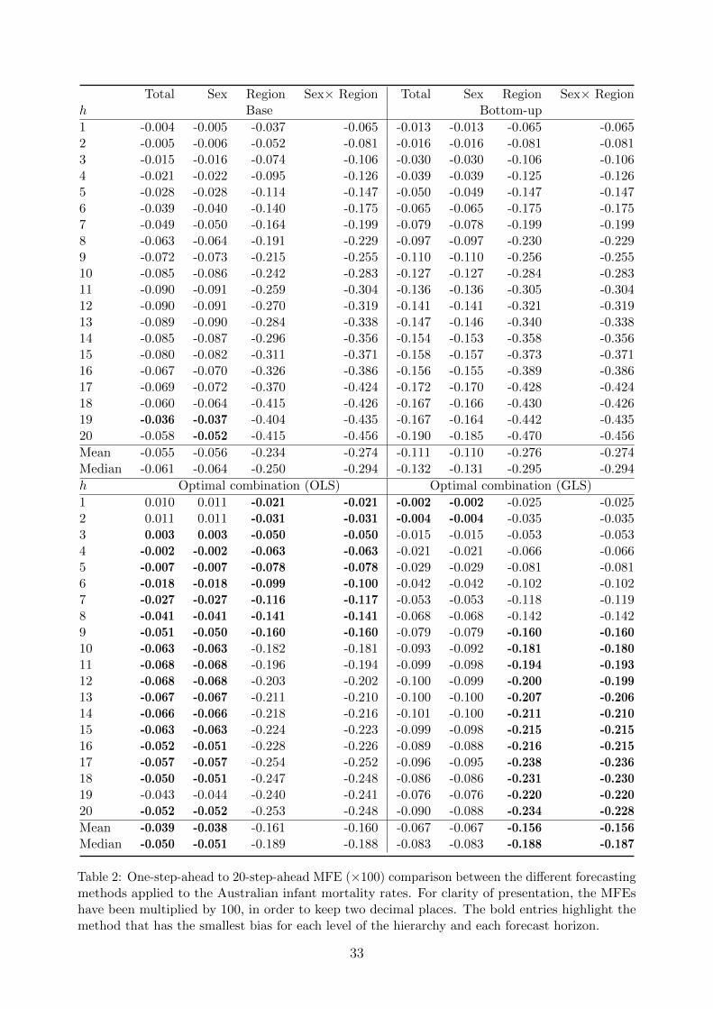
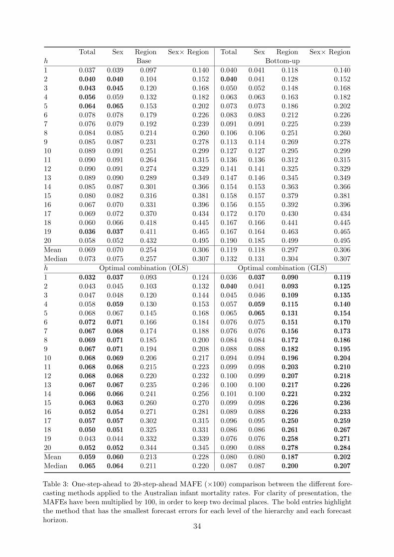
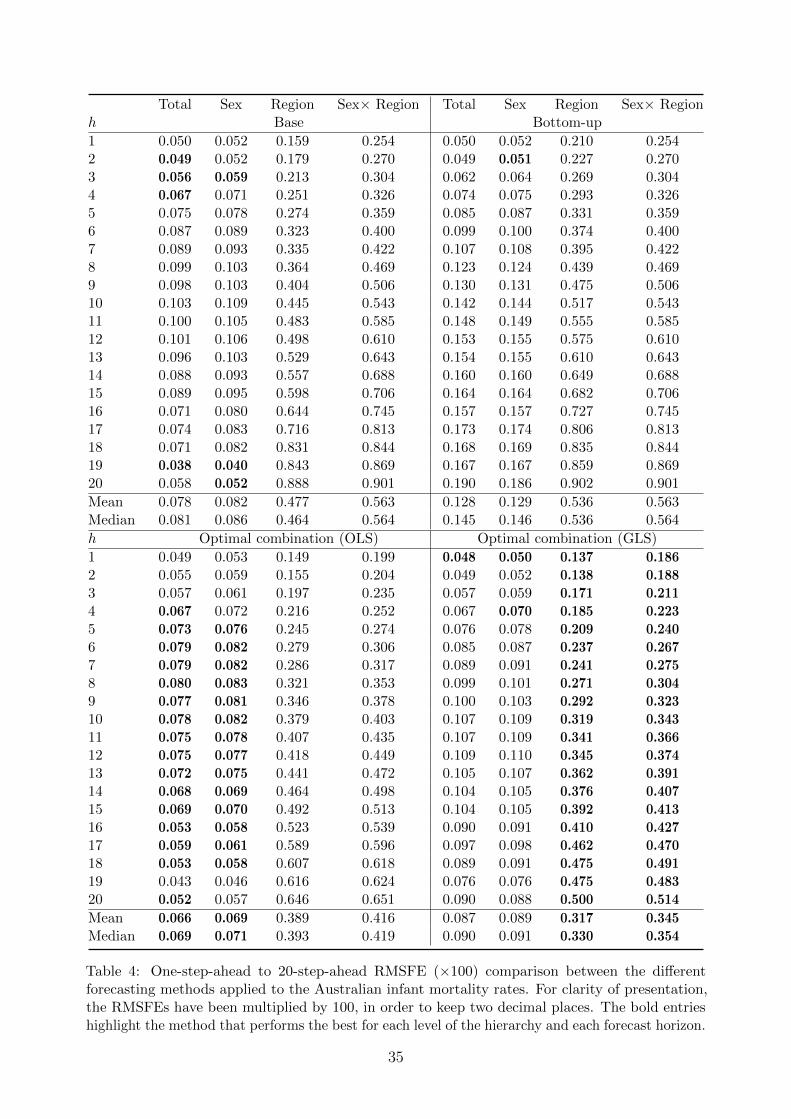
In Tables 2, 3 and 4, we present the MFE(h), MAFE(h) and RMSFE(h) for each level of

the hierarchy using the bottom-up and optimal combination methods, and a base forecasting

method (i.e., without reconciling forecasts). For ease of comparison, we highlight in bold

the method that performs the best for each level of the hierarchy and each forecast horizon,

defined as the method with the smallest MFE(h), MAFE(h) and RMSFE(h).

[Table 2 about here.]

[Table 3 about here.]

15

[Table 4 about here.]

Based on the MFE(h), the optimal combination methods generally outperform the base

and bottom-up forecasting methods. In the top level and Level 1, the optimal combination

(OLS) method has smaller forecast bias than the optimal combination (GLS) method at all

horizons, with exceptions of h = 1 and h = 2. At Level 2 and the bottom level, the forecasts

obtained from the optimal combination (OLS) method have smaller forecast bias than the

optimal combination (GLS) method at the shorter forecast horizons from h = 1 to h = 9,

but less so at the longer forecast horizons.

Based on the MAFE(h) and RMSFE(h), the optimal combination methods generally

outperform the base and bottom-up forecasting methods. In the top level and Level

1, the optimal combination (OLS) method has smaller forecast errors than the optimal

combination (GLS) method at the medium to long forecast horizons, but less so at the

shorter forecast horizons. At Level 2 and the bottom level, the forecasts obtained from the

optimal combination (GLS) method outperforms the optimal combination (OLS) method

for every forecast horizon. Averaging across all levels of a hierarchy, the point forecasts

obtained from the optimal combination (GLS) method are the most accurate in all methods

investigated, and the method produces reconciled forecasts that obey a grouped structure.

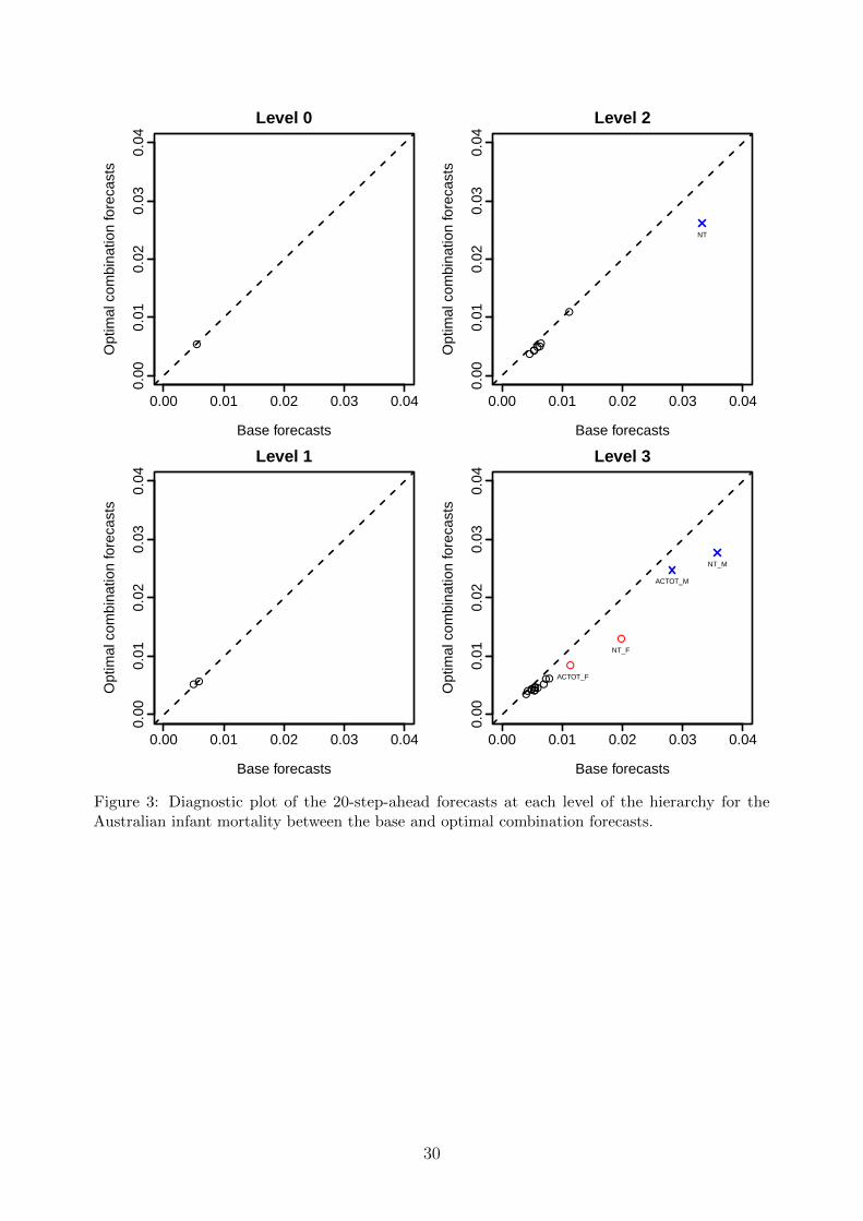
To highlight the discrepancy in point forecasts between the base forecasts and optimal

combination forecasts, we present a diagnostic plot showing the 20-step-ahead forecasts

obtained from these two methods. As an illustration, since the base forecasts provide a

foundation for the reconciled forecasts obtained from the optimal combination (OLS) method,

the diagnostic plot allows us to visualize the forecasts that are similar or different between

the two methods. As shown in Fig. 3, there are almost no difference between the two methods

at the top level and Level 1. At Level 2, there is only a difference for the NT region. At the

bottom level, the largest differences for both sexes are ACTOT and NT regions.

[Figure 3 about here.]

16

4.3 Influence of the S matrix on point forecast accuracy

The potential improvement in point forecast accuracy in the reconciliation methods relies

crucially on the accurate forecast of the S matrix. Recall that the S matrix includes ratios

of forecast exposure-at-risk. To forecast these exposure-at-risk, we again use the automatic

ARIMA method to model and forecast exposure-at-risk at the logarithmic scale. By taking

the exponential back-transformation, forecast exposure-at-risk in the original scale is obtained.

In Tables 5, 6 and 7, we compare the MAFE among the reconciliation methods with forecast

and holdout S matrices.

[Table 5 about here.]

[Table 6 about here.]

[Table 7 about here.]

At the top two levels, more accurate point forecasts can be obtained by using the holdout

S matrix. At the bottom two levels, there are comparably smaller differences in point forecast

accuracy between the forecast and actual S matrices.

5 Results of the interval forecasts

As described in Section 2.5, we constructed pointwise prediction intervals using the maximum

entropy and parametric bootstrap methods. The maximum entropy bootstrap method

generates bootstrap samples that preserve the correlation in the original time series, whereas

the parametric bootstrap method generates bootstrap forecasts for each bootstrap sample.

Based on these bootstrap forecasts, we assess the variability of point forecasts by constructing

prediction intervals based on quantiles. By averaging over all bootstrap prediction intervals,

we obtain the averaged prediction intervals. For a reasonably large level of significance

α, such as α = 0.2, averaging prediction intervals works well as we estimate the center

distribution of the quantiles. Due to heavy computational cost, there are 100 bootstrap

samples obtained by a maximum entropy bootstrap. Within each bootstrap sample, the

number of parametric bootstrap forecasts is 100.

17

Figure 4 shows the 80% pointwise averaged prediction intervals of the direct 20-steps-

ahead Australian infant mortality rate forecasts for a few selected series at each level of

the hierarchy from 1984 to 2003. At the top level, there seems to be a larger difference

in interval forecasts between the base forecasting and two grouped time-series methods.

From the middle to bottom levels, the interval forecasts are very similar between the three

methods. For the optimal combination (GLS) method, the construction of prediction interval

is hindered by the difficulty in measuring forecast uncertainty associated with Σ+, and thus

we leave this for future research.

[Figure 4 about here.]

5.1 Interval forecast evaluation

At a nominal level of 80%, prediction intervals are constructed by taking corresponding

quantiles, where the lower bound is denoted by Lω+h,j and the upper bound is denoted by

Uω+h,j for j = 1, . . . ,m and m representing the total number of series in a hierarchy. With

a pointwise prediction interval and its corresponding holdout data point in the forecasting

period, we can assess interval forecast accuracy by the interval score of Gneiting and Raftery

(2007), defined as

Sα,j

(Lω+h,j , Uω+h,j , Yω+h,j

)=(Uω+h,j − Lω+h,j

)+

2

α

(Lω+h,j − Yω+h,j

)1{Yω+h,j < Lω+h,j

}+

2

α

(Yω+h,j − Uω+h,j

)1{Yω+h,j > Uω+h,j

},

where Yω+h,j represents the holdout samples in the forecasting period for the series j, and 1{·}

is a binary indicator function. This interval score combines the halfwidth of the prediction

intervals with the coverage probability difference between the nominal and empirical coverage

probabilities. Intuitively, a forecaster is rewarded for narrow prediction intervals, but a

penalty is incurred, the size of which depends on the level of significance α, if the holdout

samples lie outside the prediction intervals.

18

For each series j at each forecast horizon, we obtain

Sα,j(h) =1

(21− h)

n+(20−h)∑ω=n

Sα,j

(Lω+h,j, Uω+h,j, Yω+h,j

), h = 1, . . . , 20,

where Sα,j

(Lω+h,j, Uω+h,j, Yω+h,j

)denotes the interval score at each level of the hierarchy

for the holdout samples in the forecasting period. By averaging the interval score Sα,j(h)

across the number of series within each level of a hierarchy, we obtain an overall assessment

of the interval forecast accuracy for each level within a hierarchy. The mean interval score is

then defined by

Sα,k(h) =1

mk

mk∑j=1

Sα,j(h),

where mk denotes the number of series at the kth level of the hierarchy, for k = 1, . . . , K.

5.2 Interval forecast accuracy of Australian infant mortality

In Table 8, we present the mean interval scores for the one-step-ahead to 20-step-ahead

forecasts at each level of the hierarchy between the three methods. For ease of comparison,

we highlight in bold the method that performs the best for each level of the hierarchy and

each forecast horizon, based on the smallest Sα,k(h).

[Table 8 about here.]

Based on the overall interval forecast accuracy Sα,k(h), the base forecasting method gives

the most accurate interval forecasts at the top three levels, but the optimal combination

method demonstrates the best interval forecast accuracy for the bottom-level series. Averaged

over all levels of the hierarchy, the base forecasting method outperforms the two grouped time-

series methods in terms of mean interval scores. A possible explanation for the inferior interval

accuracy of the grouped time-series forecasting methods is that they require the accurate

forecasts of the S matrix consisting of the forecast exposure-to-risk, which may introduce

additional forecast uncertainty. However, from a viewpoint of forecast interpretation, the

grouped time series methods produce interval forecasts that obey a grouped time-series

structure.

19

Due to the limited space, although not shown in the paper, the grouped time-series

forecasting methods can improve interval forecast accuracy in another data set, namely

the Japanese data set (Japanese Mortality Database, 2016). When the forecasts of the

exposure-to-risk are accurate, the reconciliation of interval mortality forecasts are more

accurate than the base interval forecasts. These results can be obtained upon request from

the author.

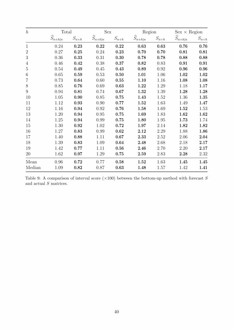
5.3 Influence of the S matrix on interval forecast accuracy

The potential improvement in interval forecast accuracy in the reconciliation methods relies

crucially on the accurate forecast of the S matrix. Recall that the S matrix includes ratios of

forecast exposure-at-risk. To obtain bootstrap forecasts of these exposure-at-risk, we use the

parametric bootstrap and maximum entropy bootstrap methods to simulate future samples of

the exposure-at-risk at the logarithmic scale. By taking the exponential back-transformation,

bootstrap forecasts of exposure-at-risk in the original scale are obtained. In Tables 9 and 10,

we compare the interval score among the reconciliation methods with forecast and holdout S

matrices.

[Table 9 about here.]

[Table 10 about here.]

At the top two levels, more accurate interval forecasts can be obtained by using the

holdout S matrix. At the Region level, the forecast S matrix gives a smaller interval score

than the holdout S matrix. This rather surprising result may due to the forecast uncertainty

associated with the mortality rates. At the bottom level, there is no difference in terms of

interval forecast accuracy between the forecast and actual S matrices.

6 Conclusions

This article adapts a bottom-up method and an optimal combination method for modeling

and forecasting grouped time series of infant mortality rates. The bottom-up method models

20

and forecasts time series at the bottom level and then aggregates to the top level using the

summing matrix. The optimal combination method optimally combines the base forecasts

through linear regression by generating a set of revised forecasts that are as close as possible

to the base forecasts but that also aggregate consistently within the group. Under a mild

assumption, regression coefficient can be estimated by either OLS or GLS estimator.

Using the regional infant mortality rates in Australia, we implemented these two grouped

time-series forecasting methods that reconcile forecasts across different levels of a hierarchy.

Furthermore, we compared the one-step-ahead to 20-step-ahead point forecast accuracy, and

found that the optimal combination method has the smallest overall forecast error in the

Australian data set considered.

Through the maximum entropy and parametric bootstrap methods, we present a means

of constructing pointwise prediction intervals for grouped time series. The maximum entropy

bootstrap is capable of mimicking the correlation within and between the original time series.

For each bootstrapped time series, we can then fit an optimal ARIMA model and generate

forecasts; from these forecasts the corresponding prediction intervals are obtained. Averaging

over all prediction intervals, we obtain averaged prediction intervals to evaluate forecast

uncertainty associated with the point forecasts.

In the Australian data set, we found that the base forecasting method gives the best

overall interval forecast accuracy, but the two grouped time-series forecasting methods

produce interval forecasts that obey a group structure and thus ease of interpretation. It is

noteworthy that the accuracy of the reconciliation methods crucially depends on the forecast

accuracy of the summing matrix. Although the forecast S matrix does not differ much from

the holdout S matrix, the reconciliation methods enjoy improved forecast accuracy with the

holdout S matrix at the top and middle levels, but less so at the bottom level.

There are several ways in which this study could be further extended and we briefly

outline five of these. First, the methods are proposed from a frequentist viewpoint, and

they can be compared with a hierarchical Bayesian method. Secondly, the methodology

can be applied to cause-specific mortality, considered in Murray and Lopez (1997), Girosi

and King (2008) and Gaille and Sherris (2015). Thirdly, the methodology can be applied to

21

other demographic data, such as population size. Fourthly, forecasts can also be obtained

by multivariate time-series forecasting methods, such as vector autoregressive models, in

order to take into account possible correlations between and within multiple time series.

Finally, the idea of grouped time series can be extended to functional time series (see Shang

and Hyndman, 2016), where each series is a time series of functions, such as age-specific

demographic rates. This work provides a natural foundation for such extensions.

22

REFERENCES

Abdel-Latif, M. E., Bajuk, B., Oei, J., Vincent, T., Sutton, L. and Lui, K. (2006), ‘Does rural

or urban residence make a difference to neonatal outcome in premature birth? A regional

study in Australia’, Archives of Disease in Childhood: Fetal & Neonatal 91(4), F251–F256.

Akaike, H. (1974), ‘A new look at the statistical model identification’, IEEE Transactions on

Automatic Control 19(6), 716–723.

Athanasopoulos, G., Ahmed, R. A. and Hyndman, R. J. (2009), ‘Hierarchical forecasts for

Australian domestic tourism’, International Journal of Forecasting 25(1), 146–166.

Chernick, M. R. and LaBudde, R. A. (2011), An introduction to bootstrap methods with

applications to R, Wiley, Hoboken, New Jersey.

Coale, A. J. and Banister, J. (1996), ‘Five decades of missing females in China’, Proceedings

of the American Philosophical Society 140(4), 421–450.

Dangerfield, B. J. and Morris, J. S. (1992), ‘Top-down or bottom-up: Aggregate versus

disaggregate extrapolations’, International Journal of Forecasting 8(2), 233–241.

Drevenstedt, G. L., Crimmins, E. M., Vasunilashorn, S. and Finch, C. E. (2008), ‘The rise

and fall of excess male infant mortality’, Proceedings of the National Academy of Sciences

of the United States of America 105(13), 5016–5021.

Flatø, M. and Kotsadam, A. (2014), Droughts and gender bias in infant mortality in

sub-Saharan Africa, Working paper 2, Department of Economics, University of Oslo.

Retrieved from: https://www.sv.uio.no/esop/forskning/aktuelt/aktuelle-saker/

2015/dokumenter/flato-kotsadam.pdf.

Fuse, K. and Crenshaw, E. M. (2006), ‘Gender imbalance in infant mortality: A cross-national

study of social structure and female infanticide’, Social Science & Medicine 62(2), 360–374.

Gaille, S. A. and Sherris, M. (2015), ‘Causes-of-death mortality: What do we know on their

dependence?’, North American Actuarial Journal 19(2), 116–128.

23

Girosi, F. and King, G. (2008), Demographic Forecasting, Princeton University Press, Prince-

ton.

Gneiting, T. and Raftery, A. E. (2007), ‘Strictly proper scoring rules, prediction and

estimation’, Journal of the American Statistical Association 102(477), 359–378.

Griffiths, P., Matthews, Z. and Hinde, A. (2000), ‘Understanding the sex ratio in India: A

simulation approach’, Demography 37(4), 477–488.

Gross, C. W. and Sohl, J. E. (1990), ‘Disaggregation methods to expedite product line

forecasting’, Journal of Forecasting 9(3), 233–254.

Hyndman, R. J. (2010), addb: Australian Demographic Data Bank. Retrieved from: http://

robjhyndman.com/software/addb/.

Hyndman, R. J., Ahmed, R. A., Athanasopoulos, G. and Shang, H. L. (2011), ‘Optimal

combination forecasts for hierarchical time series’, Computational Statistics and Data

Analysis 55(9), 2579–2589.

Hyndman, R. J. and Khandakar, Y. (2008), ‘Automatic time series forecasting: the forecast

package for R’, Journal of Statistical Software 27(3).

Hyndman, R. J., Koehler, A., Ord, J. and Snyder, R. (2008), Forecasting with Exponential

Smoothing: the State-Space Approach, Springer, New York.

Hyndman, R. J., Lee, A. J. and Wang, E. (2016), ‘Fast computation of reconciled forecasts

for hierarchical and grouped time series’, Computational Statistics and Data Analysis

97, 16–32.

Japanese Mortality Database (2016), National Institute of Population and Social Security

Research. Retrieved from http://www.ipss.go.jp (data downloaded on 18/June/2015).

Kahn, K. B. (1998), ‘Revisiting top-down versus bottom-up forecasting’, The Journal of

Business Forecasting 17(2), 14–19.

24

Kilian, L. (2001), ‘Impulse response analysis in vector autoregressions with unknown lag

order’, Journal of Forecasting 20(3), 161–179.

Kinney, W. R. (1971), ‘Predicting earnings: Entity versus subentity data’, Journal of

Accounting Research 9(1), 127–136.

Kwiatkowski, D., Phillips, P. C. B., Schmidt, P. and Shin, Y. (1992), ‘Testing the null

hypothesis of stationarity against the alternative of a unit root: How sure are we that

economic time series have a unit root?’, Journal of Econometrics 54(1-3), 159–178.

Lutkepohl, H. (2006), New Introduction to Multiple Time Series Analysis, Springer, Berlin.

Murray, C. J. L. and Lopez, A. D. (1997), ‘Alternative projections of mortality and disability

by cause 1990-2020: Global burden of disease study’, The Lancet 349(9064), 1498–1504.

Park, C. B. and Cho, N. (1995), ‘Consequences of son preference in a low-fertility society:

Imbalance of the sex ratio at birth in Korea’, Population and Development Review 21(1), 59–

84.

Pongou, R. (2013), ‘Why is infant mortality higher in boys than in girls? a new hypoth-

esis based on preconception environment and evidence from a large sample of twins’,

Demography 50(2), 421–444.

R Core Team (2016), R: A Language and Environment for Statistical Computing, R

Foundation for Statistical Computing, Vienna, Austria. Retrieved from: http://

www.R-project.org/.

Rahman, M. and DaVanzo, J. (1993), ‘Gender preference and birth spacing in Matlab,

Bangladesh’, Demography 30(3), 315–332.

Schwarzkopf, A. B., Tersine, R. J. and Morris, J. S. (1988), ‘Top-down versus bottom-up

forecasting strategies’, International Journal of Production Research 26(11), 1833–1843.

Sefton, J. and Weale, M. (2009), Reconciliation of National Income and Expenditure: Balanced

Estimates of National Income for the United Kingdom, 1920-1990, Cambridge University

Press, Cambridge.

25

Shang, H. L. and Hyndman, R. J. (2016), Grouped functional time series forecasting: an

application to age-specific mortality rates, Working paper 04/16, Monash University.

URL: http://business.monash.edu/econometrics-and-business-

statistics/research/publications/ebs/wp04-16.pdf

Shlifer, E. and Wolff, R. W. (1979), ‘Aggregation and proration in forecasting’, Management

Science 25(6), 594–603.

Stone, R., Champernowne, D. G. and Meade, J. E. (1942), ‘The precision of national income

estimates’, The Review of Economic Studies 9(2), 111–125.

Vinod, H. D. (2004), ‘Ranking mutual funds using unconventional utility theory and stochastic

dominance’, Journal of Empirical Finance 11(3), 353–377.

Vinod, H. D. and Lopez-de-Lacalle, J. (2009), ‘Maximum entropy bootstrap for time series:

the meboot R package’, Journal of Statistical Software 29(5).

Weale, M. (1988), ‘The reconciliation of values, volumes and prices in the national accounts’,

Journal of the Royal Statistical Society, Series A 151(1), 211–221.

Zellner, A. and Tobias, J. (2000), ‘A note on aggregation, disaggregation and forecasting

performance’, Journal of Forecasting 19(5), 457–469.

Zivot, E. and Wang, J. (2006), Modeling Financial Time Series with S-PLUS, Springer, New

York.

26

Appendix: Maximum entropy bootstrap algorithm

An overview of the maximum entropy bootstrap algorithm is provided for generating a

random realization of a univariate time series xt. Consult Vinod (2004) for more details and

an example. In the maximum entropy bootstrap algorithm,

1. Sort the original data in increasing order to create order statistics x(t) and store the

ordering index vector.

2. Compute intermediate points zt =x(t)+x(t+1)

2for t = 1, . . . , n−1 from the order statistics.

3. Compute the trimmed mean, denoted by mtrim of deviations xt − xt−1 among our

consecutive observations. Compute the lower limit for the left tail as z0 = x(1) −mtrim

and the upper limit for the right tail as zn = x(n) + mtrim. These limits become the

limiting intermediate points.

4. Compute the mean of the maximum entropy density within each interval such that the

“mean-preserving constraint” is satisfied. Interval means are denoted as mt. The means

for the first and last intervals have simpler formulas:

m1 = 0.75x(1) + 0.25x(2)

mk = 0.25x(k−1) + 0.5x(k) + 0.25x(k+1), k = 2, . . . , n

mn = 0.25x(n−1) + 0.75x(n)

5. Generate random numbers from Uniform[0, 1], compute sample quantiles of the maxi-

mum entropy density at those points and sort them.

6. Re-order the sorted sample quantiles by using the ordering index of Step 1. This

recovers the time dependence relationships of the originally observed data.

7. Repeat Steps 2 to 6 several times.

27

Australia

R1

F M

R2

F M

· · · R8

F M

Figure 1: A two-level hierarchical tree diagram, with eight regions. In the top level, we have themortality for Australia; in Level 1, total mortality of Australia can be disaggregated by eightregions; in Level 2, total mortality of each region can be disaggregated by sex within each region.

28

Level 0

Year

Mor

talit

y ra

te

1940 1960 1980 2000

0.01

0.02

0.03

0.04

Total

1940 1960 1980 2000

0.01

0.02

0.03

0.04

Level 1

Year

Mor

talit

y ra

te

FemaleMale

1940 1960 1980 2000

0.01

0.02

0.03

0.04

Level 2

YearM

orta

lity

rate

Region 1 (Victoria)Region 2 (New South Wales)

1940 1960 1980 2000

0.00

0.01

0.02

0.03

0.04

0.05

0.06

Level 3

Year

Mor

talit

y ra

te

Region 1 (Female)Region 1 (Male)

Figure 2: Infant mortality rates can be disaggregated by sex in Level 1, region in Level 2, and sexand region in Level 3. For clarity of presentation, we plot only two regions in Level 2, and twosexes of region 1 in Level 3. Based on the data from 1933 to 1983, the bottom-up method is usedto produce 20-steps-ahead forecasts from 1984 to 2003 across different levels of the hierarchy. Thethicker line(s) represent(s) the historical data, while the thinner line(s) represent(s) the forecasts.

29

●

0.00 0.01 0.02 0.03 0.04

0.00

0.01

0.02

0.03

0.04

Level 0

Base forecasts

Opt

imal

com

bina

tion

fore

cast

s

●●●●●

●

●

0.00 0.01 0.02 0.03 0.04

0.00

0.01

0.02

0.03

0.04

Level 2

Base forecastsO

ptim

al c

ombi

natio

n fo

reca

sts

NT

●●

0.00 0.01 0.02 0.03 0.04

0.00

0.01

0.02

0.03

0.04

Level 1

Base forecasts

Opt

imal

com

bina

tion

fore

cast

s

●●●●●● ●●

●●●

●

0.00 0.01 0.02 0.03 0.04

0.00

0.01

0.02

0.03

0.04

Level 3

Base forecasts

Opt

imal

com

bina

tion

fore

cast

s

●

●

ACTOT_F

ACTOT_M

NT_F

NT_M

Figure 3: Diagnostic plot of the 20-step-ahead forecasts at each level of the hierarchy for theAustralian infant mortality between the base and optimal combination forecasts.

30

1985 1990 1995 2000

0.00

40.

006

0.00

80.

010

0.01

2Level 0: Total mortality

Year

Mor

talit

y ra

te

ObservationsIndependent prediction intervalsBottom−up prediction intervalsOptimal combination prediction intervals

1985 1990 1995 2000

0.00

40.

006

0.00

80.

010

0.01

2

Level 2: Total mortality in state Victoria

Year

Mor

talit

y ra

te

1985 1990 1995 2000

0.00

40.

006

0.00

80.

010

0.01

2

Level 1: Female mortality

Year

Mor

talit

y ra

te

1985 1990 1995 2000

0.00

40.

006

0.00

80.

010

0.01

2

Level 3: Female mortality in state Victoria

Year

Mor

talit

y ra

te

Figure 4: Based on the Australian infant mortality data from 1933 to 1983, we produce 20-steps-ahead prediction intervals for years 1984 to 2003, at the nominal coverage probability of 80%. Forease of presentation, we show the 80% prediction intervals for a few selected series at each level ofthe hierarchy.

31

Level Number of seriesAustralia 1Sex 2State 8Sex × State 16Total 27

Table 1: Hierarchy of Australian infant mortality rates.

32

Total Sex Region Sex× Region Total Sex Region Sex× Regionh Base Bottom-up

1 -0.004 -0.005 -0.037 -0.065 -0.013 -0.013 -0.065 -0.0652 -0.005 -0.006 -0.052 -0.081 -0.016 -0.016 -0.081 -0.0813 -0.015 -0.016 -0.074 -0.106 -0.030 -0.030 -0.106 -0.1064 -0.021 -0.022 -0.095 -0.126 -0.039 -0.039 -0.125 -0.1265 -0.028 -0.028 -0.114 -0.147 -0.050 -0.049 -0.147 -0.1476 -0.039 -0.040 -0.140 -0.175 -0.065 -0.065 -0.175 -0.1757 -0.049 -0.050 -0.164 -0.199 -0.079 -0.078 -0.199 -0.1998 -0.063 -0.064 -0.191 -0.229 -0.097 -0.097 -0.230 -0.2299 -0.072 -0.073 -0.215 -0.255 -0.110 -0.110 -0.256 -0.25510 -0.085 -0.086 -0.242 -0.283 -0.127 -0.127 -0.284 -0.28311 -0.090 -0.091 -0.259 -0.304 -0.136 -0.136 -0.305 -0.30412 -0.090 -0.091 -0.270 -0.319 -0.141 -0.141 -0.321 -0.31913 -0.089 -0.090 -0.284 -0.338 -0.147 -0.146 -0.340 -0.33814 -0.085 -0.087 -0.296 -0.356 -0.154 -0.153 -0.358 -0.35615 -0.080 -0.082 -0.311 -0.371 -0.158 -0.157 -0.373 -0.37116 -0.067 -0.070 -0.326 -0.386 -0.156 -0.155 -0.389 -0.38617 -0.069 -0.072 -0.370 -0.424 -0.172 -0.170 -0.428 -0.42418 -0.060 -0.064 -0.415 -0.426 -0.167 -0.166 -0.430 -0.42619 -0.036 -0.037 -0.404 -0.435 -0.167 -0.164 -0.442 -0.43520 -0.058 -0.052 -0.415 -0.456 -0.190 -0.185 -0.470 -0.456

Mean -0.055 -0.056 -0.234 -0.274 -0.111 -0.110 -0.276 -0.274Median -0.061 -0.064 -0.250 -0.294 -0.132 -0.131 -0.295 -0.294

h Optimal combination (OLS) Optimal combination (GLS)

1 0.010 0.011 -0.021 -0.021 -0.002 -0.002 -0.025 -0.0252 0.011 0.011 -0.031 -0.031 -0.004 -0.004 -0.035 -0.0353 0.003 0.003 -0.050 -0.050 -0.015 -0.015 -0.053 -0.0534 -0.002 -0.002 -0.063 -0.063 -0.021 -0.021 -0.066 -0.0665 -0.007 -0.007 -0.078 -0.078 -0.029 -0.029 -0.081 -0.0816 -0.018 -0.018 -0.099 -0.100 -0.042 -0.042 -0.102 -0.1027 -0.027 -0.027 -0.116 -0.117 -0.053 -0.053 -0.118 -0.1198 -0.041 -0.041 -0.141 -0.141 -0.068 -0.068 -0.142 -0.1429 -0.051 -0.050 -0.160 -0.160 -0.079 -0.079 -0.160 -0.16010 -0.063 -0.063 -0.182 -0.181 -0.093 -0.092 -0.181 -0.18011 -0.068 -0.068 -0.196 -0.194 -0.099 -0.098 -0.194 -0.19312 -0.068 -0.068 -0.203 -0.202 -0.100 -0.099 -0.200 -0.19913 -0.067 -0.067 -0.211 -0.210 -0.100 -0.100 -0.207 -0.20614 -0.066 -0.066 -0.218 -0.216 -0.101 -0.100 -0.211 -0.21015 -0.063 -0.063 -0.224 -0.223 -0.099 -0.098 -0.215 -0.21516 -0.052 -0.051 -0.228 -0.226 -0.089 -0.088 -0.216 -0.21517 -0.057 -0.057 -0.254 -0.252 -0.096 -0.095 -0.238 -0.23618 -0.050 -0.051 -0.247 -0.248 -0.086 -0.086 -0.231 -0.23019 -0.043 -0.044 -0.240 -0.241 -0.076 -0.076 -0.220 -0.22020 -0.052 -0.052 -0.253 -0.248 -0.090 -0.088 -0.234 -0.228

Mean -0.039 -0.038 -0.161 -0.160 -0.067 -0.067 -0.156 -0.156Median -0.050 -0.051 -0.189 -0.188 -0.083 -0.083 -0.188 -0.187

Table 2: One-step-ahead to 20-step-ahead MFE (×100) comparison between the different forecastingmethods applied to the Australian infant mortality rates. For clarity of presentation, the MFEshave been multiplied by 100, in order to keep two decimal places. The bold entries highlight themethod that has the smallest bias for each level of the hierarchy and each forecast horizon.

33

Total Sex Region Sex× Region Total Sex Region Sex× Regionh Base Bottom-up

1 0.037 0.039 0.097 0.140 0.040 0.041 0.118 0.1402 0.040 0.040 0.104 0.152 0.040 0.041 0.128 0.1523 0.043 0.045 0.120 0.168 0.050 0.052 0.148 0.1684 0.056 0.059 0.132 0.182 0.063 0.063 0.163 0.1825 0.064 0.065 0.153 0.202 0.073 0.073 0.186 0.2026 0.078 0.078 0.179 0.226 0.083 0.083 0.212 0.2267 0.076 0.079 0.192 0.239 0.091 0.091 0.225 0.2398 0.084 0.085 0.214 0.260 0.106 0.106 0.251 0.2609 0.085 0.087 0.231 0.278 0.113 0.114 0.269 0.27810 0.089 0.091 0.251 0.299 0.127 0.127 0.295 0.29911 0.090 0.091 0.264 0.315 0.136 0.136 0.312 0.31512 0.090 0.091 0.274 0.329 0.141 0.141 0.325 0.32913 0.089 0.090 0.289 0.349 0.147 0.146 0.345 0.34914 0.085 0.087 0.301 0.366 0.154 0.153 0.363 0.36615 0.080 0.082 0.316 0.381 0.158 0.157 0.379 0.38116 0.067 0.070 0.331 0.396 0.156 0.155 0.392 0.39617 0.069 0.072 0.370 0.434 0.172 0.170 0.430 0.43418 0.060 0.066 0.418 0.445 0.167 0.166 0.441 0.44519 0.036 0.037 0.411 0.465 0.167 0.164 0.463 0.46520 0.058 0.052 0.432 0.495 0.190 0.185 0.499 0.495

Mean 0.069 0.070 0.254 0.306 0.119 0.118 0.297 0.306Median 0.073 0.075 0.257 0.307 0.132 0.131 0.304 0.307

h Optimal combination (OLS) Optimal combination (GLS)

1 0.032 0.037 0.093 0.124 0.036 0.037 0.090 0.1192 0.043 0.045 0.103 0.132 0.040 0.041 0.093 0.1253 0.047 0.048 0.120 0.144 0.045 0.046 0.109 0.1354 0.058 0.059 0.130 0.153 0.057 0.059 0.115 0.1405 0.068 0.067 0.145 0.168 0.065 0.065 0.131 0.1546 0.072 0.071 0.166 0.184 0.076 0.075 0.151 0.1707 0.067 0.068 0.174 0.188 0.076 0.076 0.156 0.1738 0.069 0.071 0.185 0.200 0.084 0.084 0.172 0.1869 0.067 0.071 0.194 0.208 0.088 0.088 0.182 0.19510 0.068 0.069 0.206 0.217 0.094 0.094 0.196 0.20411 0.068 0.068 0.215 0.223 0.099 0.098 0.203 0.21012 0.068 0.068 0.220 0.232 0.100 0.099 0.207 0.21813 0.067 0.067 0.235 0.246 0.100 0.100 0.217 0.22614 0.066 0.066 0.241 0.256 0.101 0.100 0.221 0.23215 0.063 0.063 0.260 0.270 0.099 0.098 0.226 0.23616 0.052 0.054 0.271 0.281 0.089 0.088 0.226 0.23317 0.057 0.057 0.302 0.315 0.096 0.095 0.250 0.25918 0.050 0.051 0.325 0.331 0.086 0.086 0.261 0.26719 0.043 0.044 0.332 0.339 0.076 0.076 0.258 0.27120 0.052 0.052 0.344 0.345 0.090 0.088 0.278 0.284

Mean 0.059 0.060 0.213 0.228 0.080 0.080 0.187 0.202Median 0.065 0.064 0.211 0.220 0.087 0.087 0.200 0.207

Table 3: One-step-ahead to 20-step-ahead MAFE (×100) comparison between the different fore-casting methods applied to the Australian infant mortality rates. For clarity of presentation, theMAFEs have been multiplied by 100, in order to keep two decimal places. The bold entries highlightthe method that has the smallest forecast errors for each level of the hierarchy and each forecasthorizon.

34

Total Sex Region Sex× Region Total Sex Region Sex× Regionh Base Bottom-up

1 0.050 0.052 0.159 0.254 0.050 0.052 0.210 0.2542 0.049 0.052 0.179 0.270 0.049 0.051 0.227 0.2703 0.056 0.059 0.213 0.304 0.062 0.064 0.269 0.3044 0.067 0.071 0.251 0.326 0.074 0.075 0.293 0.3265 0.075 0.078 0.274 0.359 0.085 0.087 0.331 0.3596 0.087 0.089 0.323 0.400 0.099 0.100 0.374 0.4007 0.089 0.093 0.335 0.422 0.107 0.108 0.395 0.4228 0.099 0.103 0.364 0.469 0.123 0.124 0.439 0.4699 0.098 0.103 0.404 0.506 0.130 0.131 0.475 0.50610 0.103 0.109 0.445 0.543 0.142 0.144 0.517 0.54311 0.100 0.105 0.483 0.585 0.148 0.149 0.555 0.58512 0.101 0.106 0.498 0.610 0.153 0.155 0.575 0.61013 0.096 0.103 0.529 0.643 0.154 0.155 0.610 0.64314 0.088 0.093 0.557 0.688 0.160 0.160 0.649 0.68815 0.089 0.095 0.598 0.706 0.164 0.164 0.682 0.70616 0.071 0.080 0.644 0.745 0.157 0.157 0.727 0.74517 0.074 0.083 0.716 0.813 0.173 0.174 0.806 0.81318 0.071 0.082 0.831 0.844 0.168 0.169 0.835 0.84419 0.038 0.040 0.843 0.869 0.167 0.167 0.859 0.86920 0.058 0.052 0.888 0.901 0.190 0.186 0.902 0.901

Mean 0.078 0.082 0.477 0.563 0.128 0.129 0.536 0.563Median 0.081 0.086 0.464 0.564 0.145 0.146 0.536 0.564

h Optimal combination (OLS) Optimal combination (GLS)

1 0.049 0.053 0.149 0.199 0.048 0.050 0.137 0.1862 0.055 0.059 0.155 0.204 0.049 0.052 0.138 0.1883 0.057 0.061 0.197 0.235 0.057 0.059 0.171 0.2114 0.067 0.072 0.216 0.252 0.067 0.070 0.185 0.2235 0.073 0.076 0.245 0.274 0.076 0.078 0.209 0.2406 0.079 0.082 0.279 0.306 0.085 0.087 0.237 0.2677 0.079 0.082 0.286 0.317 0.089 0.091 0.241 0.2758 0.080 0.083 0.321 0.353 0.099 0.101 0.271 0.3049 0.077 0.081 0.346 0.378 0.100 0.103 0.292 0.32310 0.078 0.082 0.379 0.403 0.107 0.109 0.319 0.34311 0.075 0.078 0.407 0.435 0.107 0.109 0.341 0.36612 0.075 0.077 0.418 0.449 0.109 0.110 0.345 0.37413 0.072 0.075 0.441 0.472 0.105 0.107 0.362 0.39114 0.068 0.069 0.464 0.498 0.104 0.105 0.376 0.40715 0.069 0.070 0.492 0.513 0.104 0.105 0.392 0.41316 0.053 0.058 0.523 0.539 0.090 0.091 0.410 0.42717 0.059 0.061 0.589 0.596 0.097 0.098 0.462 0.47018 0.053 0.058 0.607 0.618 0.089 0.091 0.475 0.49119 0.043 0.046 0.616 0.624 0.076 0.076 0.475 0.48320 0.052 0.057 0.646 0.651 0.090 0.088 0.500 0.514

Mean 0.066 0.069 0.389 0.416 0.087 0.089 0.317 0.345Median 0.069 0.071 0.393 0.419 0.090 0.091 0.330 0.354

Table 4: One-step-ahead to 20-step-ahead RMSFE (×100) comparison between the differentforecasting methods applied to the Australian infant mortality rates. For clarity of presentation,the RMSFEs have been multiplied by 100, in order to keep two decimal places. The bold entrieshighlight the method that performs the best for each level of the hierarchy and each forecast horizon.

35

h Total Sex Region Sex × Region

Sn+h|n Sn+h Sn+h|n Sn+h Sn+h|n Sn+h Sn+h|n Sn+h

1 0.0399 0.0399 0.0406 0.0405 0.1175 0.1173 0.1397 0.13972 0.0404 0.0404 0.0407 0.0406 0.1275 0.1277 0.1516 0.15163 0.0504 0.0496 0.0515 0.0504 0.1482 0.1483 0.1681 0.16814 0.0629 0.0611 0.0627 0.0608 0.1625 0.1625 0.1816 0.18165 0.0728 0.0695 0.0727 0.0692 0.1862 0.1861 0.2022 0.20226 0.0831 0.0804 0.0831 0.0802 0.2120 0.2123 0.2264 0.22647 0.0908 0.0843 0.0907 0.0840 0.2253 0.2254 0.2387 0.23878 0.1059 0.0970 0.1058 0.0967 0.2511 0.2514 0.2598 0.25989 0.1126 0.1016 0.1145 0.1026 0.2693 0.2693 0.2782 0.278210 0.1270 0.1111 0.1266 0.1108 0.2953 0.2943 0.2990 0.299011 0.1364 0.1169 0.1360 0.1163 0.3125 0.3115 0.3145 0.314512 0.1414 0.1184 0.1411 0.1179 0.3252 0.3245 0.3289 0.328913 0.1467 0.1188 0.1464 0.1183 0.3454 0.3435 0.3487 0.348714 0.1536 0.1188 0.1527 0.1183 0.3627 0.3613 0.3661 0.366115 0.1576 0.1167 0.1566 0.1161 0.3787 0.3752 0.3806 0.380616 0.1560 0.1078 0.1547 0.1073 0.3915 0.3903 0.3961 0.396117 0.1720 0.1147 0.1703 0.1141 0.4302 0.4267 0.4341 0.434118 0.1673 0.1065 0.1659 0.1059 0.4413 0.4381 0.4453 0.445319 0.1670 0.0966 0.1643 0.0961 0.4632 0.4566 0.4651 0.465120 0.1898 0.1222 0.1847 0.1218 0.4988 0.4861 0.4951 0.4951

Mean 0.1187 0.0936 0.1181 0.0934 0.2972 0.2954 0.3060 0.3060Median 0.1317 0.1041 0.1313 0.1043 0.3039 0.3029 0.3067 0.3067

Table 5: A comparison of MAFE (×100) between the bottom-up method with forecast S and actualS matrices.

36

h Total Sex Region Sex×Region

Sn+h|n Sn+h Sn+h|n Sn+h Sn+h|n Sn+h Sn+h|n Sn+h

1 0.0324 0.0324 0.0374 0.0377 0.0927 0.0926 0.1238 0.12382 0.0434 0.0438 0.0452 0.0456 0.1026 0.1028 0.1322 0.13223 0.0466 0.0472 0.0484 0.0488 0.1198 0.1196 0.1442 0.14424 0.0578 0.0579 0.0594 0.0595 0.1299 0.1299 0.1535 0.15355 0.0678 0.0678 0.0671 0.0673 0.1455 0.1455 0.1675 0.16756 0.0717 0.0707 0.0713 0.0703 0.1656 0.1656 0.1842 0.18427 0.0672 0.0658 0.0675 0.0658 0.1742 0.1747 0.1884 0.18848 0.0695 0.0644 0.0706 0.0672 0.1849 0.1849 0.1998 0.19989 0.0674 0.0606 0.0709 0.0630 0.1945 0.1940 0.2080 0.208010 0.0681 0.0556 0.0686 0.0574 0.2065 0.2056 0.2167 0.216711 0.0683 0.0520 0.0685 0.0536 0.2149 0.2144 0.2232 0.223212 0.0682 0.0493 0.0678 0.0489 0.2204 0.2202 0.2324 0.232413 0.0672 0.0446 0.0669 0.0465 0.2354 0.2347 0.2463 0.246314 0.0662 0.0384 0.0656 0.0381 0.2412 0.2403 0.2555 0.255515 0.0632 0.0397 0.0626 0.0424 0.2596 0.2581 0.2700 0.270016 0.0516 0.0173 0.0542 0.0269 0.2707 0.2701 0.2814 0.281417 0.0573 0.0192 0.0569 0.0222 0.3019 0.3010 0.3151 0.315118 0.0499 0.0205 0.0508 0.0331 0.3253 0.3226 0.3309 0.330919 0.0429 0.0123 0.0442 0.0161 0.3325 0.3308 0.3391 0.339120 0.0518 0.0025 0.0515 0.0294 0.3438 0.3366 0.3446 0.3446

Mean 0.0589 0.0431 0.0598 0.0470 0.2131 0.2122 0.2278 0.2278Median 0.0647 0.0459 0.0641 0.0477 0.2107 0.2100 0.2200 0.2200

Table 6: A comparison of MAFE (×100) between the optimal combination method (the OLSestimator) with forecast S and actual S matrices.

37

h Total Sex Region Sex × Region

Sn+h|n Sn+h Sn+h|n Sn+h Sn+h|n Sn+h Sn+h|n Sn+h

1 0.0363 0.0362 0.0366 0.0367 0.0897 0.0897 0.1189 0.11892 0.0404 0.0406 0.0407 0.0410 0.0935 0.0936 0.1247 0.12473 0.0450 0.0450 0.0462 0.0461 0.1089 0.1087 0.1354 0.13544 0.0567 0.0569 0.0587 0.0587 0.1151 0.1151 0.1400 0.14005 0.0646 0.0649 0.0651 0.0650 0.1313 0.1311 0.1538 0.15386 0.0756 0.0739 0.0752 0.0738 0.1512 0.1512 0.1705 0.17057 0.0761 0.0737 0.0765 0.0737 0.1561 0.1569 0.1733 0.17338 0.0840 0.0788 0.0839 0.0796 0.1725 0.1726 0.1864 0.18649 0.0879 0.0811 0.0880 0.0808 0.1822 0.1821 0.1948 0.194810 0.0939 0.0849 0.0941 0.0855 0.1961 0.1953 0.2043 0.204311 0.0986 0.0871 0.0981 0.0866 0.2032 0.2028 0.2101 0.210112 0.0995 0.0864 0.0992 0.0860 0.2069 0.2071 0.2178 0.217813 0.1004 0.0846 0.1001 0.0842 0.2166 0.2151 0.2258 0.225814 0.1007 0.0810 0.0999 0.0805 0.2210 0.2204 0.2318 0.231815 0.0990 0.0757 0.0982 0.0753 0.2262 0.2241 0.2357 0.235716 0.0888 0.0623 0.0880 0.0620 0.2264 0.2258 0.2332 0.233217 0.0957 0.0648 0.0947 0.0645 0.2498 0.2486 0.2590 0.259018 0.0865 0.0546 0.0864 0.0550 0.2614 0.2593 0.2667 0.266719 0.0764 0.0395 0.0760 0.0394 0.2580 0.2553 0.2709 0.270920 0.0899 0.0594 0.0875 0.0596 0.2776 0.2707 0.2837 0.2837

Mean 0.0798 0.0666 0.0797 0.0667 0.1872 0.1863 0.2018 0.2018Median 0.0872 0.0693 0.0869 0.0693 0.1996 0.1991 0.2072 0.2072

Table 7: A comparison of MAFE (×100) between the optimal combination method (the GLSestimator) with forecast S and actual S matrices.

38

Total Sex Region Sex× Region Total Sex Region Sex× Regionh Base Bottom-up

1 0.17 0.18 0.55 0.77 0.24 0.22 0.63 0.762 0.17 0.21 0.59 0.81 0.27 0.24 0.70 0.813 0.21 0.26 0.65 0.88 0.36 0.31 0.78 0.884 0.23 0.28 0.69 0.91 0.46 0.38 0.82 0.915 0.26 0.32 0.74 0.96 0.54 0.45 0.89 0.966 0.31 0.35 0.80 1.02 0.65 0.53 1.01 1.027 0.34 0.37 0.81 1.08 0.73 0.60 1.10 1.088 0.37 0.39 0.87 1.18 0.85 0.68 1.22 1.189 0.35 0.38 0.93 1.28 0.94 0.74 1.32 1.2810 0.37 0.40 1.02 1.36 1.05 0.85 1.43 1.3611 0.35 0.38 1.07 1.47 1.12 0.90 1.52 1.4912 0.36 0.38 1.07 1.52 1.16 0.92 1.58 1.5213 0.29 0.34 1.13 1.62 1.20 0.95 1.69 1.6214 0.26 0.29 1.16 1.74 1.25 0.99 1.80 1.7315 0.30 0.31 1.17 1.84 1.30 1.02 1.97 1.8216 0.24 0.24 1.26 1.89 1.27 0.99 2.12 1.8817 0.24 0.24 1.46 2.05 1.40 1.11 2.33 2.0618 0.25 0.25 1.78 2.19 1.39 1.09 2.48 2.1819 0.24 0.24 1.96 2.19 1.42 1.11 2.46 2.2020 0.25 0.24 2.19 2.36 1.62 1.29 2.59 2.28

Mean 0.28 0.30 1.10 1.46 0.96 0.77 1.52 1.45Median 0.26 0.30 1.04 1.42 1.09 0.87 1.48 1.42

h Optimal combination (OLS)1 0.27 0.21 0.60 0.722 0.28 0.23 0.68 0.763 0.37 0.30 0.76 0.834 0.48 0.37 0.82 0.865 0.55 0.44 0.91 0.926 0.66 0.54 1.05 0.977 0.74 0.59 1.15 1.028 0.87 0.69 1.27 1.119 0.95 0.75 1.37 1.2010 1.06 0.85 1.49 1.2711 1.13 0.89 1.59 1.3612 1.16 0.90 1.64 1.4113 1.19 0.92 1.73 1.5014 1.22 0.95 1.83 1.5815 1.24 0.96 2.00 1.6716 1.21 0.91 2.16 1.7117 1.31 1.01 2.44 1.8818 1.31 1.00 2.66 2.0919 1.34 1.01 2.78 2.1920 1.56 1.22 2.99 2.40Mean 0.94 0.74 1.59 1.37Median 1.09 0.87 1.54 1.32

Table 8: One-step-ahead to 20-step-ahead interval score (×100) comparison between the differentforecasting methods applied to the Australian infant mortality rates. Note that the slight discrepancybetween the base forecasts and bottom-up forecasts at the bottom level is due to different randomseeds used in bootstrapping.

39

h Total Sex Region Sex × Region

Sn+h|n Sn+h Sn+h|n Sn+h Sn+h|n Sn+h Sn+h|n Sn+h

1 0.24 0.23 0.22 0.22 0.63 0.63 0.76 0.762 0.27 0.25 0.24 0.23 0.70 0.70 0.81 0.813 0.36 0.33 0.31 0.30 0.78 0.78 0.88 0.884 0.46 0.42 0.38 0.37 0.82 0.83 0.91 0.915 0.54 0.49 0.45 0.43 0.89 0.92 0.96 0.966 0.65 0.59 0.53 0.50 1.01 1.06 1.02 1.027 0.73 0.64 0.60 0.55 1.10 1.16 1.08 1.088 0.85 0.76 0.69 0.63 1.22 1.29 1.18 1.179 0.94 0.81 0.74 0.67 1.32 1.39 1.28 1.2810 1.05 0.90 0.85 0.75 1.43 1.52 1.36 1.3511 1.12 0.93 0.90 0.77 1.52 1.63 1.49 1.4712 1.16 0.94 0.92 0.76 1.58 1.69 1.52 1.5313 1.20 0.94 0.95 0.75 1.69 1.83 1.62 1.6214 1.25 0.94 0.99 0.75 1.80 1.95 1.73 1.7415 1.30 0.92 1.02 0.72 1.97 2.14 1.82 1.8216 1.27 0.83 0.99 0.62 2.12 2.29 1.88 1.8617 1.40 0.88 1.11 0.67 2.33 2.52 2.06 2.0418 1.39 0.83 1.09 0.64 2.48 2.68 2.18 2.1719 1.42 0.77 1.11 0.56 2.46 2.70 2.20 2.1720 1.62 0.97 1.29 0.75 2.59 2.83 2.28 2.32

Mean 0.96 0.72 0.77 0.58 1.52 1.63 1.45 1.45Median 1.09 0.82 0.87 0.63 1.48 1.57 1.42 1.41

Table 9: A comparison of interval score (×100) between the bottom-up method with forecast Sand actual S matrices.

40

h Total Sex Region Sex × Region

Sn+h|n Sn+h Sn+h|n Sn+h Sn+h|n Sn+h Sn+h|n Sn+h

1 0.27 0.27 0.21 0.23 0.60 0.61 0.72 0.732 0.28 0.27 0.23 0.23 0.68 0.69 0.76 0.763 0.37 0.35 0.30 0.30 0.76 0.78 0.83 0.844 0.48 0.46 0.37 0.37 0.82 0.85 0.86 0.875 0.55 0.51 0.44 0.43 0.91 0.94 0.92 0.926 0.66 0.61 0.54 0.52 1.05 1.09 0.97 0.987 0.74 0.67 0.59 0.56 1.15 1.19 1.02 1.038 0.87 0.79 0.69 0.64 1.27 1.33 1.11 1.129 0.95 0.85 0.75 0.69 1.37 1.44 1.20 1.2110 1.06 0.94 0.85 0.77 1.49 1.58 1.27 1.2811 1.13 0.98 0.89 0.79 1.59 1.67 1.36 1.3612 1.16 0.98 0.90 0.78 1.64 1.75 1.41 1.4113 1.19 0.98 0.92 0.77 1.73 1.88 1.50 1.5014 1.22 0.97 0.95 0.76 1.83 1.99 1.58 1.5815 1.24 0.94 0.96 0.73 2.00 2.19 1.67 1.6716 1.21 0.85 0.91 0.63 2.16 2.34 1.71 1.6917 1.31 0.90 1.01 0.67 2.44 2.62 1.88 1.8718 1.31 0.84 1.00 0.64 2.66 2.84 2.09 2.0219 1.34 0.77 1.01 0.55 2.78 2.94 2.19 2.1620 1.56 0.98 1.22 0.74 2.99 3.17 2.40 2.38

Mean 0.94 0.75 0.74 0.59 1.59 1.70 1.37 1.37Median 1.09 0.85 0.87 0.64 1.54 1.63 1.32 1.32

Table 10: A comparison of interval score (×100) between the optimal combination method withforecast S and actual S matrices.

41