Hakan Cebeci Nu¨lifer Ozdemir¨ Sec¸il S¸entorun · or examine the effect on the motion of...
31
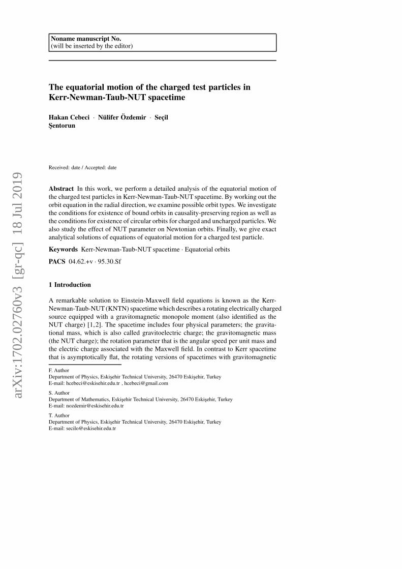
arXiv:1702.02760v3 [gr-qc] 18 Jul 2019 Noname manuscript No. (will be inserted by the editor) The equatorial motion of the charged test particles in Kerr-Newman-Taub-NUT spacetime Hakan Cebeci · N¨ ulifer ¨ Ozdemir · Sec ¸il S ¸ entorun Received: date / Accepted: date Abstract In this work, we perform a detailed analysis of the equatorial motion of the charged test particles in Kerr-Newman-Taub-NUT spacetime. By working out the orbit equation in the radial direction, we examine possible orbit types. We investigate the conditions for existence of bound orbits in causality-preserving region as well as the conditions for existence of circular orbits for charged and uncharged particles. We also study the effect of NUT parameter on Newtonian orbits. Finally, we give exact analytical solutions of equations of equatorial motion for a charged test particle. Keywords Kerr-Newman-Taub-NUT spacetime · Equatorial orbits PACS 04.62.+v · 95.30.Sf 1 Introduction A remarkable solution to Einstein-Maxwell field equations is known as the Kerr- Newman-Taub-NUT (KNTN) spacetime which describes a rotating electrically charged source equipped with a gravitomagnetic monopole moment (also identified as the NUT charge) [1,2]. The spacetime includes four physical parameters; the gravita- tional mass, which is also called gravitoelectric charge; the gravitomagnetic mass (the NUT charge); the rotation parameter that is the angular speed per unit mass and the electric charge associated with the Maxwell field. In contrast to Kerr spacetime that is asymptotically flat, the rotating versions of spacetimes with gravitomagnetic F. Author Department of Physics, Eskis ¸ehir Technical University, 26470 Eskis ¸ehir, Turkey E-mail: [email protected] , [email protected] S. Author Department of Mathematics, Eskis ¸ehir Technical University, 26470 Eskis ¸ehir, Turkey E-mail: [email protected] T. Author Department of Physics, Eskis ¸ehir Technical University, 26470 Eskis ¸ehir, Turkey E-mail: [email protected]
Transcript of Hakan Cebeci Nu¨lifer Ozdemir¨ Sec¸il S¸entorun · or examine the effect on the motion of...
arX
iv:1
702.
0276
0v3
[gr
-qc]
18
Jul 2
019
Noname manuscript No.(will be inserted by the editor)
The equatorial motion of the charged test particles in
Kerr-Newman-Taub-NUT spacetime
Hakan Cebeci · Nulifer Ozdemir · Secil
Sentorun
Received: date / Accepted: date
Abstract In this work, we perform a detailed analysis of the equatorial motion of
the charged test particles in Kerr-Newman-Taub-NUT spacetime. By working out the
orbit equation in the radial direction, we examine possible orbit types. We investigate
the conditions for existence of bound orbits in causality-preserving region as well as
the conditions for existence of circular orbits for charged and uncharged particles. We
also study the effect of NUT parameter on Newtonian orbits. Finally, we give exact
analytical solutions of equations of equatorial motion for a charged test particle.
Keywords Kerr-Newman-Taub-NUT spacetime · Equatorial orbits
PACS 04.62.+v · 95.30.Sf
1 Introduction
A remarkable solution to Einstein-Maxwell field equations is known as the Kerr-
Newman-Taub-NUT (KNTN) spacetime which describes a rotating electrically charged
source equipped with a gravitomagnetic monopole moment (also identified as the
NUT charge) [1,2]. The spacetime includes four physical parameters; the gravita-
tional mass, which is also called gravitoelectric charge; the gravitomagnetic mass
(the NUT charge); the rotation parameter that is the angular speed per unit mass and
the electric charge associated with the Maxwell field. In contrast to Kerr spacetime
that is asymptotically flat, the rotating versions of spacetimes with gravitomagnetic
F. Author
Department of Physics, Eskisehir Technical University, 26470 Eskisehir, Turkey
E-mail: [email protected] , [email protected]
S. Author
Department of Mathematics, Eskisehir Technical University, 26470 Eskisehir, Turkey
E-mail: [email protected]
T. Author
Department of Physics, Eskisehir Technical University, 26470 Eskisehir, Turkey
E-mail: [email protected]
2 Hakan Cebeci et al.
monopole moment (Kerr-Taub-NUT and Kerr-Newman-Taub- NUT spacetimes) are
asymptotically non-flat due to existence of the NUT charge. Although the Kerr-Taub-
NUT and the KNTN spacetimes involve no curvature singularities, there exist conical
singularities on the axis of symmetry. As discussed in [3], one can get rid off conical
singularities by imposing a periodicity condition over the time coordinate. However,
this inevitably leads to the emergence of closed timelike curves in the spacetime that
makes it unphysical in the context of causality. To make the spacetime with the NUT
charge physically relevant, one can investigate the global analysis of such spacetimes
as in [4,5]. In this manner, an alternative physical interpretation of the spacetime with
NUT charge has been given in [4] where the NUT metric is interpreted as a semi-
infinite massless source of angular momentum (involving the singularity on the axis
where θ = π). Despite some unpleasing physical features of Taub-NUT spacetimes,
the physical meaning of gravitomagnetic monopole moment and the physical interac-
tions including NUT parameter have been comprehensively investigated. In [6,7], the
physical meaning of NUT parameter has been exploited by examining the twisting
effect of monopole moment on the orbit of the light rays. In [8,9], interaction of the
massless scalar fields with gravitomagnetic monopole moment and gravitomagnetic
effects regarding the NUT parameter have been investigated respectively. In [10,11,
12], some physical applications have been illustrated in the background of space-
times involving the NUT parameter; namely in [10], gyromagnetic ratio related to
KNTN spacetime has been obtained, in [11], hidden symmetries of Kerr-Taub-NUT
spacetime in Kaluza-Klein theory have been explored, while in [12], acceleration of
particles on the background of Kerr-Taub-NUT spacetime has been studied.
In order to detect the existence of a NUT source in the universe, one can either
investigate the effect of this parameter on the motion of light or examine the effect
on the motion of massive test particles. To accomplish and exploit such effect, one
can study geodesics or the orbital motion on the background of spacetimes involving
the NUT parameter. Such a study was initiated by [13] where the Schwarzschild type
geodesics on the background of NUT spacetime has been examined by concluding
that such geodesics lie on the cones with the apex located at r = 0. Later in [14],
a comprehensive analytic investigation of complete and incomplete geodesics in a
(non-rotating) Taub-NUT spacetime has been realised. On the other hand, the motion
of particles in a Kerr-Taub-NUT gravitational source immersed in a magnetic field
has been investigated in [15]. In addition, in [16], energy extraction process (Penrose
process) has been examined in rotating Kerr-Taub-NUT spacetime. In the work [17],
an analytic expression for shadows (known as a special lensing property) of a Kerr-
Newman-NUT spacetime has been obtained while examining the motion of photon in
this background. In a recent work [18], circular geodesics of uncharged test particles
has been analysed in KNTN spacetime while in [19], timelike circular geodesics in
(non-rotating) NUT spacetime has been studied while also discussing the Von Zeipel
cylinders with respect to stationary observers and determining the relation of such
cylinders to inertial forces. Recently the motion of charged particles has been inves-
tigated in an Einstein-Maxwell spacetime with NUT parameter [20], where in such
a spacetime the causality violation has also been examined. Very recently in [21],
the equations of motion of a test particle have been examined in a special class of
Kerr-Newman-NUT spacetime background where a specific relation is imposed on

The equatorial motion of the charged test particles in Kerr-Newman-Taub-NUT spacetime 3
the NUT charge, electric charge and rotation parameter of the spacetime. In addition
to study of geodesics of light and massive test particles in spacetimes with NUT pa-
rameter, gravitational waves can also be viewed as a possible third method to detect
a NUT charge in the universe [22].
This work is devoted to the study of equatorial orbits of charged massive test
particle in KNTN spacetime. In previous works, the motion of charged massive test
particles has been analytically investigated in Reissner-Nordstrom [23,25], Reissner-
Nordstrom-(Anti)-de-Sitter [26], Kerr-Newman [27] and Kerr-Newman-AdS (in f (R)gravity) [28] respectively. Our aim is to make a detailed analysis of the equatorial mo-
tion of the charged massive test particles in KNTN spacetime and to investigate the
effect of the rotation and the NUT parameters on the equatorial motion. In fact, we
have recently examined the non-equatorial orbital motion of charged massive test par-
ticles in KNTN background in [29], where we have briefly mentioned the conditions
for the existence of the equatorial orbits in rotating NUT spacetime without making
a detailed analysis and investigation of such orbits. In this work, we present a more
elaborate analysis of the equatorial motion of charged massive test particles in KNTN
spacetime where we particularly examine the existence of bound and circular orbits
over equatorial plane. We should remark that, the study of equatorial orbits in rotating
NUT spacetime deserves a separate care and investigation. As is also mentioned in
[9], the equatorial orbits in rotating NUT spacetimes do not exist for arbitrary rotation
and the NUT parameters. In [29], we have shown that, there exist equatorial orbits in
such spacetimes provided that either the NUT parameter should vanish or a certain
relation between the angular momentum and the energy of the test particle and the
rotation parameter should exist (for arbitrary NUT parameter). In this work, we con-
centrate on the latter, i.e. we examine the equatorial orbits of the charged test particles
in which such a relation holds. We examine the possible orbit types depending on the
value of the energy of the test particle while a special investigation is devoted to the
study of the existence of bound orbits in causality-preserving region and existence of
circular orbits. To our knowledge, the study of circular orbits in rotating spacetimes
has been initiated by Bardeen et al. [30] for Kerr spacetime. Later, the investigation
of the existence of circular geodesics has been accomplished in Kerr-Newman space-
time [31,32]. A detailed investigation of such orbits has also been realised in Kerr-de
Sitter and Kerr-Anti-de Sitter spacetimes including cosmological constant together
with mass and rotation parameters [33,34]. In our study, we derive necessary con-
ditions for the existence of equatorial bound orbits in causality-preserving region as
well as the existence circular orbits in KNTN spacetime. In addition, we study the
effect of the NUT parameter on the equatorial Newtonian orbits. Finally, we present
the analytical solutions of the equations of motion over the equatorial plane by ex-
pressing them in terms of Weierstrass ℘, σ , and ζ functions. We also provide plots
of possible orbit types and calculate the perihelion shift for an equatorial bound orbit.
Organisation of the paper is as follows: In Section 2, we provide an introduction
to KNTN spacetime. In Section 3, we obtain the governing equations of equatorial
motion of the charged test particles. In Section 4, we make a comprehensive anal-
ysis of possible orbit types. In the same section, we examine the conditions for the
existence of equatorial bound orbits in causality-preserving region and existence of
circular orbits. Moreover, the Newtonian limit of the equatorial orbits are discussed

4 Hakan Cebeci et al.
while investigating the physical effect of the NUT parameter on the Newtonian orbits
as well. In Section 5, we present the exact analytic solutions of the equatorial orbits
while also calculating the perihelion shift for an equatorial bound orbit. We end up
with some comments and conclusions.
2 Kerr-Newman-Taub-NUT spacetime
The KNTN spacetime is known as a stationary rotating solution of the Einstein-
Maxwell field equations. The metric is asymptotically non-flat due to the existence
of a NUT charge which is also identified as the gravitomagnetic monopole moment.
In Boyer-Lindquist coordinates, KNTN spacetime can be written as (with asymptot-
ically non-flat structure),
g =−∆
Σ(dt − χdϕ)2 +Σ
(
dr2
∆+ dθ 2
)
+sin2 θ
Σ
(
adt − (r2 + ℓ2 + a2)dϕ)2
(1)
where
Σ = r2 +(ℓ+ acosθ )2,
∆ = r2 − 2Mr+ a2 − ℓ2+Q2, (2)
χ = asin2 θ − 2ℓcosθ .
Here, M can be identified as the parameter related to the physical mass of the grav-
itational source, a is associated with its angular momentum per unit mass while ℓspecifies gravitomagnetic monopole moment of the source which is also identified as
the NUT charge. Also, Q is specified as the electric charge. The electromagnetic field
of the source can be expressed as the potential 1-form
A = Aµdxµ =−Qr
Σ(dt − χdϕ). (3)
We use geometrized units such that c = 1 and G = 1. As is also remarked in [5],
there exist two types of singularities related to that spacetime; one coming from the
singularities of the metric components and the other resulting from vanishing of the
determinant of the metric. The former results in the singularities at the spacetime
coordinates where ∆(r) = 0 and Σ(r,θ ) = 0 producing singularities at the horizons
r = r∓ and a conical singularity (at r = 0 and cosθ =− ℓa
with ℓ2 < a2) respectively.
The latter occurs at θ = 0 and θ = π . When the NUT parameter ℓ = 0, the conical
singularity obviously turns into the equatorial ring singularity at r = 0 and θ = π2
.
We further remark that, the metric singularities related to radial coordinate exist at
the locations
r± = M±√
M2 − a2 + ℓ2 −Q2, (4)
where ∆(r±) = 0 provided that M2 − a2 + ℓ2 −Q2 ≥ 0. The singularity r− can be
identified as inner (or Cauchy) horizon while r+ can be named as outer (or event)

The equatorial motion of the charged test particles in Kerr-Newman-Taub-NUT spacetime 5
horizon. It can also be seen that, the spacetime allows a family of locally non-rotating
observers which rotate with coordinate angular velocity given by
Ω =− gtϕ
gϕϕ=
∆ χ − asin2 θ (r2 + ℓ2 + a2)
∆ χ2 − sin2 θ (r2 + ℓ2 + a2)2(5)
which is known as the frame dragging effect arising due to the presence of the off-
diagonal component gtϕ of the metric. We also remark that at the outermost singular-
ity r+, the angular velocity can be calculated as
Ω+ =−(
gtϕ
gϕϕ
)∣
∣
∣
∣
r=r+
=a
r2++ ℓ2 + a2
· (6)
It can also be easily seen that the Killing vectors ξ(t) and ξ(ϕ) generate two constants
of motion namely the energy and the angular momentum of the test particle. More-
over, it is straightforward to show that the Killing vector ξ = ξ(t)+Ω+ξ(ϕ) becomes
null at the metric singularity where r = r+.
3 The equations of motion
In this section, we examine the motion of charged test particle over the equatorial
plane in KNTN spacetime. Traditionally, to obtain the equation of motions over the
equatorial plane, one usually starts with the Lagrangian expression [36] and sim-
ply substitute θ = π2
in the resulting expressions. However, this standard technique
cannot be directly applied for the KNTN spacetime since as is explicitly illustrated
in [9] and [29], the existence of the equatorial orbits requires either the vanishing
of the NUT parameter (ℓ = 0) or a specific relation between the rotation parame-
ter a, the energy E, the angular momentum L of the test particle to hold. For that
reason, one cannot directly substitute θ = π2
for the equatorial orbital motion. In-
stead, to get the field equations over the equatorial plane, one should start with the
celebrated Hamilton-Jacobi equation, and then obtain the condition for the existence
of equatorial orbits and substitute such a relation in the remaining governing equa-
tions. Therefore, governing orbit equations over equatorial plane can be obtained by
using Hamilton-Jacobi method discussed in [29]. To summarize, one can start with
Hamilton-Jacobi equation [37,38,39,40]
2∂S
∂τ= gµν
(
∂S
∂xµ− qAµ
)(
∂S
∂xν− qAν
)
(7)
where τ denotes an affine parameter and q is the electric charge of the test particle.
Also, the existence of the timelike Killing vector ξ(t) and spacelike Killing vector
ξ(ϕ) for the KNTN spacetime (1) lead to the identifications
Pt =−E, Pϕ = L, (8)
where the expression for the canonical momenta Pµ can be written as
Pµ =∂S
∂xµ= mgµν
dxν
dτ+ qAµ. (9)

6 Hakan Cebeci et al.
Here m is the mass of the test particle while E and L correspond to the energy and
the angular momentum of the test particle. Now, it has been shown in [29] that if the
relation
L =a(2E2 − 1)
2E, (E 6= 0), (10)
with
E =E
m, L =
L
m(11)
is imposed between the rotation parameter a, rescaled energy E and the angular mo-
mentum L of the test particle, the particle is confined to move over the equatorial
plane. One can infer from this relation that if a 6= 0, but 2E2 = 1 (L = 0), the orbits of
the charged test particle can be identified as the motion with vanishing orbital angular
momentum. One more crucial remark is that, if 2E2 > 1, L > 0 implying that equa-
torial orbits are direct (or prograde) orbits (L and a have the same sign also assuming
that a > 0). If on the other hand, 2E2 < 1, L < 0 which implies that the orbits are
retrograde orbits (L and a have opposite signs).
In addition, to get the complete governing equations of motion over the equatorial
plane, one can introduce a new time parameter λ as in [41,42] such that
dλ
dτ=
1
Σ(12)
and substitute θ = π2
, L = a(2E2−1)2E
together with Carter constant Km2 = ℓ2 + a2
4E2 in
the orbit equations presented in [29]. To conclude, the governing orbit equations take
the following form:(
dr
dλ
)2
= Pr(r), (13)
(
dr
dϕ
)2
=∆ 2(r)Pr(r)
a2([
E(r2 + ℓ2)+ a2
2E− qQr
]
− ∆ (r)2E
)2, (14)
(
dr
dt
)2
=∆ 2(r)Pr(r)
(
(r2 + a2 + ℓ2)[
E(r2 + ℓ2)+ a2
2E− qQr
]
− a2∆ (r)2E
)2(15)
where we define
Pr(r) =
[
E(r2 + ℓ2)+a2
2E− qQr
]2
−∆(r)
(
r2 + ℓ2 +a2
4E2
)
. (16)
Here q = qm
. Now writing the radial potential Pr(r) over the equatorial plane in the
form
Pr(r) = r4
(
E
(
1+ℓ2
r2
)
+a2
2Er2− qQ
r
)2
−∆(r)
(
r2 + ℓ2 +a2
4E2
)
, (17)
The equatorial motion of the charged test particles in Kerr-Newman-Taub-NUT spacetime 7
one can physically interpret the term a2
2Er2 as the spin orbit coupling potential arising
from the orbital motion of the test particle around the rotating spacetime (due to rela-
tion aLr2 = a2
r2 (E − 12E) over equatorial plane) and term
qQr
as electrostatic interaction
potential (between charge of test particle and charge of the spacetime).
Finally, we note that the equations (13)-(15) have been obtained under the assumption
that ℓ 6= 0. When ℓ = 0 (vanishing of the NUT parameter), one does not require the
relation (10), since relation (10) should be used for the existence of equatorial orbits
in a spacetime with NUT parameter (i.e in a spacetime with ℓ 6= 0). Therefore, for
ℓ = 0, one should consider the equations of motion outlined in [29]. Indeed, if one
substitutes ℓ = 0 (taking θ = π2
for the equatorial orbits) in the equations of motion
presented in [29], one obtains the orbit equations for the charged test particle in Kerr-
Newman spacetime where in this case, the angular momentum L and energy E of the
test particle appear as independent parameters of the radial potential (see also [27]).
3.1 Ergoregion in KNTN spacetime
Before moving to next section, we should note that there exists another feature of
KNTN spacetime that is worth mentioning. Such a property that deserves special in-
vestigation is the existence of an ergoregion (or existence of ergosurface) and it is
seen as characteristic of stationary spacetimes. The existence of an ergoregion in sta-
tionary spacetimes require that norm of timelike Killing field (i.e metric component
gtt ) becomes positive. It means that the coordinate t in this region is no longer a time-
like coordinate but it becomes spacelike. We note that in recent works [43] and [44],
the characteristics of such a region on the equatorial plane of Kerr spacetime has been
examined in detail. For KNTN spacetime, in the region where the relation
∆ − a2 sin2 θ < 0 (18)
holds, the metric component gtt becomes positive. Therefore, the location of ergosur-
face for KNTN spacetime, also known as the stationary limit surface, can be obtained
from
r2 − 2Mr+ a2 cos2 θ +Q2 − ℓ2 = 0 (19)
whose solution leads to
r∓e (θ ) = M∓√
M2 + ℓ2 −Q2 − a2 cos2 θ .
Here r−e (θ ) can be identified as inner ergosurface while r+e (θ ) is identified as outer
ergosurface. One can immediately see that the relation
r−e < r− < r+ < r+e (20)
holds between inner and outer ergosurfaces and Cauchy (inner horizon r− ) and event
(outer horizon r+) horizons. We note that ergosurfaces coincide with Cauchy and
event horizons when θ = 0 and θ = π . When θ = π2
, i.e over the equatorial plane of
KNTN spacetime, expression for ergosurfaces takes the form
r∓e = M∓√
M2 + ℓ2 −Q2 . (21)
8 Hakan Cebeci et al.
It is interesting to observe that ergosurfaces over equatorial plane of KNTN spacetime
are independent of spacetime rotation parameter a but they depend on other spacetime
parameters. Another remarkable feature of the ergoregion is that static observers can-
not exist in ergoregion (where r+ < r < r+e ) of equatorial KNTN spacetime. It means
that there is no static observer with drdτ = 0, dθ
dτ = 0 anddϕdτ = 0 where τ denotes
proper time. Referring to our previous work [29] , this fact can be seen from angular
velocity expression
dϕ
dτ=
a
(r2 + ℓ2)∆
(
1
2E(a2 −∆)+ E(r2 + ℓ2)− qQr
)
(22)
such that expression never vanishes in ergoregion where r+ < r < r+e . Looking at this
expression, owing to
a2 −∆ > 0
in the ergoregion r+ < r < r+e over equatorial plane, expression is strictly positive for
an uncharged particle (q = 0) that enters into ergoregion with positive energy. For a
charged particle with positive energy, expression is positive provided that
4E2ℓ2 − q2Q2 > 0 . (23)
In addition, angular velocity expression has same sign with spacetime rotation pa-
rameter a which implies that test particles that enter into ergoregion are forced to
rotate in direction of rotation of KNTN black hole. Obviously, it is zero when a = 0
where spacetime is static in that case.
Also, another characteristics of ergoegion that deserves further mentioning is that
Killing vector ξ(t) =∂∂ t
becomes spacelike [35,36]. Physically, it means that, in the
ergoregion, energy E of the test particle measured with respect to an observer at
spatial infinity can be negative. Then from physical point of view, an immediate con-
sequence of existence of such a region between event horizon and stationary limit
surface is that it can allow Penrose process that results in the extraction of energy
from KNTN black hole [16]. In addition, it should be noted that negative energy par-
ticles within ergoregion cannot exit from ergoregion, while particles with positive
energy can enter that region and exit from ergoregion. The fact that energy of test
particle in ergoregion can be negative also requires that angular momentum L of par-
ticle measured with respect to an observer at spatial infinity can be negative as well.
Especially, if one considers circular motion in ergoregion, the energy E and angular
momentum L turns out to be negative [36,43] . As a final comment, for the motion
over equatorial plane of KNTN spacetime, the negativity of angular momentum also
agrees with constraint relation (10) such that when E < 0 (provided that 2E2 > 1),
it requires that L < 0 as well. At this point, we should point out that a more detailed
investigation of motion in ergoregion of KNTN spacetime as done for Kerr spacetime
in [43,44], could be subject of another future work.
4 Analysis of the orbit configurations
In this section, we make a classification of possible orbit configurations with respect
to radial motion expressed by the radial potential Pr(r). Next, we make a detailed
The equatorial motion of the charged test particles in Kerr-Newman-Taub-NUT spacetime 9
investigation of the existence of bound orbits in causality-preserving region and exis-
tence of circular orbits. Finally, we illustrate the effect of the NUT parameter on the
equatorial Newtonian orbits.
First, one can easily see that radial potential Pr(r) is a fourth order polynomial in r
with real coefficients, where it can be expressed in the form
Pr(r) = B0 +B1r+B2r2 +B3r3 +B4r4 (24)
where the coefficients read
B4 = E2 − 1, (25)
B3 = 2(M− EqQ), (26)
B2 = 2E2ℓ2 +Q2(q2 − 1)− a2
4E2, (27)
B1 = 2(M− qQE)
(
ℓ2 +a2
4E2
)
− qQa2
2E, (28)
and
B0 = ℓ4E2 +(ℓ2 −Q2)
(
ℓ2 +a2
4E2
)
. (29)
Also we note that the radial motion is possible if Pr(r) ≥ 0. Then, according to the
roots of the radial polynomial Pr(r), one can identify the following orbit types in gen-
eral [14,45]:
i. Bound orbit: When the particle moves in a region r2 ≤ r ≤ r1 (either r1 > r2 > 0
or r2 < r1 < 0), the motion of the particle can be identified as bound where the point
r = 0 is not crossed. On the other hand if the bound orbit exists in a region r2 < r < r1
with r2 < 0 and r1 > 0, the orbit can be identified as crossover bound orbit where the
point r = 0 is crossed twice. In addition, the bound orbit can be identified as many-
world bound orbit [23,24], if r2 < r− and r1 > r+. In such a case the test particle
moves in a bound orbit stretching from one part of the spacetime region into another
part several times where particle crosses two metric singularities at r = r− and r = r+and turns back at r = r2. The bound orbits are possible if Pr(r) has four real roots or
two real roots (with two complex roots) or two real double roots or one real triple root
and one real root. In such cases, depending on the real roots of the radial potential,
there may exist one or two bound regions.
ii. Circular Orbit: The orbit is called circular if Pr(r) has a real double root at r = rc
where rc denotes the radius of the circular orbit.
iii. Escape orbit: The orbit is called escape if the particle moves either in the range
r1 < r < ∞ (with r1 > 0) or −∞ < r < r2 (with r2 < 0) where the point r = 0 is not
crossed. The orbit can be identified as crossover escape orbit if the particle moves
either in the range r1 < r < ∞ (with r1 < 0) or −∞ < r < r2 (with r2 > 0). In such
a case the particle crosses the point r = 0 twice. If the motion of the particle is re-
stricted to be either in the interval r1 < r < ∞ with r1 < r− < r+ or −∞ < r < r2 with

10 Hakan Cebeci et al.
r− < r+ < r2, then the orbit can be referred as two-world escape orbit. In such a case,
the particle passes through from one part of the spacetime region into another part
where again the particle will cross two metric singularities twice. Likewise, escape
orbits can arise when Pr(r) has four real roots or two real roots (with two complex
roots) or two real double roots or one real triple root and one real root. We note that
there may exist one or two escape orbits depending on the number of real roots.
iv. Transit orbit: The orbit is said to be transit if the particle starts from ∓∞, crosses
r = 0 and moves to ±∞. This can be possible if Pr(r) has no real roots. It is obvious
that if Pr(0)> 0, the particle can cross the point r = 0. This can happen if
B0 = ℓ4E2 +(ℓ2 −Q2)
(
ℓ2 +a2
4E2
)
> 0. (30)
It is seen that if ℓ≥ Q, the particle can always cross the point r = 0.
One can further examine the possible orbit configurations depending on the value of
the energy of the test particle:
1. The case for E2 6= 1:
If Pr(r) has four different real roots, one can obtain two bound orbits for E2 < 1,
while for E2 > 1 one can get one bound and two escape orbits. If Pr(r) has two dif-
ferent real zeros (and two complex conjugate roots), then one can get only one bound
orbit for E2 < 1, while for E2 > 1, one can obtain two escape orbits. If Pr(r) has no
real zeros, then the radial motion is not possible for E2 < 1 since Pr(r) < 0 for all r,
while one can get a transit orbit for E2 > 1 since r →∓∞, Pr(r)→ ∞ .
2. The case for E2 = 1:
For E2 = 1, Pr(r) becomes a third order polynomial. Moreover, the orbit configu-
rations can change according to the sign of the coefficient of the first term (i.e. the
coefficient of r3). For both of the cases M > qQ and M < qQ, if Pr(r) has three dis-
tinct real roots, there exist one bound and one escape orbits. If on the other hand
Pr(r) has only one real root (together with two complex roots), then there exists only
one escape orbit. For this case, for M > qQ, escape orbit is observed in the inter-
val r1 ≤ r < +∞ while for M < qQ, the escape orbit can be realised in the interval
−∞ < r ≤ r1 where r1 is the real root of Pr(r).It is also of interest to examine the case where E2 = 1 and M = qQ. For this special
case, Pr(r) becomes a second order polynomial:(
2ℓ2 +Q2(q2 − 1)− a2
4
)
r2 − a2
2qQr+ ℓ2 +(ℓ2 −Q2)
(
ℓ2 +a2
4
)
= 0. (31)
In this case, the orbit configurations can modify according to the sign of the coeffi-
cient of r2 term. Then, if
2ℓ2 +Q2(q2 − 1)− a2
4> 0, (32)

The equatorial motion of the charged test particles in Kerr-Newman-Taub-NUT spacetime 11
one can obtain two escape or a transit orbit according to whether Pr(r) has two dif-
ferent real zeros (or one double zero) or no zeros respectively. If on the other hand,
2ℓ2 +Q2(q2 − 1)− a2
4< 0, (33)
one can get one bound orbit or no radial motion according to whether Pr(r) has two
different real zeros or no zeros respectively.
As a final remark, to see the effect of NUT parameter on the formation of possi-
ble orbit configurations, it will be useful to obtain the plots of the effective potential
Pr(r) for different values of NUT parameter and to make an analysis of possible or-
bit configurations as NUT parameter changes. Such plots are given in Figures 1-3.
In these plots, the parameters can be chosen to obtain a physically acceptable ra-
dial motion (i.e Pr(r) ≥ 0). Looking at plots, one can observe that for case E2 > 1,
for positively charged particle, while bound and circular orbits are formed for suffi-
ciently small and critical values of NUT parameter (for the critical values ℓ= 0.67272
and ℓ = 0.758142 of the NUT parameter circular orbits can form), transit orbits are
observed as ℓ increases. However, for negatively charged particle, (for same energy
and spacetime parameters chosen) while escape orbits are formed for small values
of NUT parameter, as in motion of charged test particle, a transit orbit is observed
for sufficiently large values of ℓ. On the other hand, for uncharged particle, all re-
sulting orbit configurations are transit for same energy and spacetime parameters. As
for case E2 < 1, for a positively charged particle, while two bound and circular or-
bits can be formed for sufficiently small and critical values of NUT parameter (for
the critical value ℓ = 0.437329 of the NUT parameter, a circular orbit forms), only
one bound orbit can be observed as value of NUT parameter increases. On the other
hand, for negatively charged and uncharged particles, only one bound orbit (actually
a many-world bound) is formed for all values of NUT parameter (again for same
energy and spacetime parameters). Finally, for case E2 = 1, for motion of positively
charged test particle, while bound (a many-world bound) and circular orbits can be
observed for sufficiently small and critical values of NUT parameter (for the critical
value ℓ = 0.747708 of the NUT parameter, again a circular orbit forms), a crossover
escape orbit (for region −∞ < r < r1, r1 being the root of radial polynomial) can be
formed for sufficiently large values of ℓ. On the other hand, for a negatively charged
particle, while one can observe one bound and escape orbits for small values of NUT
parameter, one can encounter crossover escape orbits (for region r1 < r < ∞) for
sufficiently large values of NUT parameter. As for an uncharged particle, for same
spacetime parameters chosen, only crossover escape orbits are observed for all values
of NUT parameter.
4.1 Existence of bound orbits in causality-preserving region
It is obvious that the particle moves in a bound orbit if the radial motion is constrained
in the interval r2 ≤ r ≤ r1 (r2 and r1 are finite) where r2 and r1 correspond to turning
points of radial potential Pr(r) such that Pr(r2) = Pr(r1) = 0. From physical point of

12 Hakan Cebeci et al.
(a) Effective potential for radial motion of positively charged test
particle (q = 10)
(b) Effective potential for radial motion of nega-
tively charged test particle (q =−5)
(c) Effective potential for radial motion of un-
charged test particle (q = 0)
Fig. 1: Effective radial potentials for different values of NUT parameter ℓ when E > 1.
Black solid, black dashed, black dotted and black dot-dashed curves are obtained for
ℓ= 0.4, ℓ= 0.672720, ℓ= 0.758142 and ℓ= 1.2 respectively. In all the plots, we take
E = 2, M = 1, Q = 0.4 and a = 0.9.
view, it will be of great interest to investigate existence of bound orbits in causality-
preserving region. As discussed in [36], extending spacetime to allow negative r val-
ues, it is certain that causality is violated in the domain for which gϕϕ < 0 and ϕbecomes a time-like coordinate. Hence, the domains for which gϕϕ > 0 and space-
like character of ϕ-coordinate is preserved can be identified as causality-preserving
regions. For KNTN spacetime, it is obvious from metric structure that gϕϕ
∣
∣
θ= π2> 0
for r > r+ which implies that the region where r > r+ is a causality-preserving region.
Of course, for KNTN spacetime, there exist other regions where metric component
gϕϕ
∣
∣
θ= π2> 0. However, as done in [46], we concentrate on existence of bound or-
bits in the causality-preserving region where r > r+ (i.e outside outer singularity). In
what follows, we will investigate conditions for which a bound orbit exists in region
where r > r+ for E2 > 1, E2 < 1 and E2 = 1. We should remark that it has been
shown in [46] for Kerr spacetime that for E2 > 1 there exist no bound orbit in causal-
ity preserving region (bound orbit in region where r > r+). To make an analysis of
such a bound motion for our spacetime, we follow a similar procedure outlined in

The equatorial motion of the charged test particles in Kerr-Newman-Taub-NUT spacetime 13
(a) Effective potential for radial motion of
positively charged test particle (q = 5)
(b) Effective potential for radial motion of
negatively charged test particle (q =−2)
(c) Effective potential for radial motion of uncharged
test particle (q = 0)
Fig. 2: Effective radial potentials for different values of NUT parameter ℓ when E <1. Black solid, black dashed and black dotted curves are obtained for ℓ = 0.1, ℓ =0.437329 and ℓ= 0.8 respectively. In all the plots, we take E = 0.3, M = 1, Q = 0.4and a = 0.9.
[46]. In this sense, the conditions for the existence of bound orbits can be determined
by using Descartes’ rule of sign. According to Descartes’ rule of sign, a polynomial
possessing real coefficients can not have more positive roots than the number of vari-
ations of sign in its coefficients. First of all, the conditions that we will obtain will
imply that a radial bound interval r2 ≤ r ≤ r1 may exist such that for that region,
Pr(r) > 0 and r2 > r+. Now following a similar procedure as done in [46], we can
affect a transformation r = R+ r+, where r+ describes the metric singularity (i.e.
∆(r+) = 0), assuming that at least one region of binding exists where r > r+. To this
end, we express Pr(r) in terms of new variable R. Then in terms of R, we obtain
PR(R) = A4R4 +A3R3 +A2R2 +A1R+A0 (34)
where
A0 =1
4E2
[
a2 + 2E(
ℓ2E + r+(Er+− qQ))]2
, (35)
A1 =a2
2E2
[
M− 2qQE + r+(4E2 − 1)]
+ 2ℓ2[
M− qQE + r+(2E2 − 1)]

14 Hakan Cebeci et al.
(a) Effective potential for radial motion of positively charged test par-
ticle (q = 10)
(b) Effective potential for radial motion of
negatively charged test particle (q =−12)
(c) Effective potential for radial motion of un-
charged test particle (q = 0)
Fig. 3: Effective radial potentials for different values of NUT parameter ℓ when E =1. Black solid, black dashed and black dotted curves are obtained for ℓ = 0.4, ℓ =0.747708 and ℓ = 1.2 respectively. In all the plots, we take M = 1, Q = 0.4 and
a = 0.9.
+2r+[
q2Q2 + r+(M− 3qQE)+ r2+(2E2 − 1)
]
, (36)
A2 = q2Q2 + a2
(
1− 1
4E2
)
+ ℓ2(2E2 − 1)
+2r+(2M− 3qQE)+ r2+(6E2 − 5), (37)
A3 = 2[
M− qQE + 2r+(E2 − 1)
]
(38)
and
A4 = E2 − 1. (39)
At this stage, let us consider in what conditions this polynomial has positive roots
(which will lead to the existence of bound orbit for r > r+). We remark that A0 > 0.

The equatorial motion of the charged test particles in Kerr-Newman-Taub-NUT spacetime 15
Then according to Descartes’ rule of sign if A4 > 0 (E2 > 1), a bound region for
r > r+ may be realised under the conditions
A1 < 0, A2 > 0, A3 < 0 (40)
since we also have A0 > 0. Then four variations of sign would be possible and there-
fore there may exist four (distinct) real positive roots for PR(R). If the above inequal-
ity conditions are simultaneously met, we have the possibility of having a bound
motion for E2 > 1 in the region where r > r+. Such a bound orbit for E > 1 and
r > r+ can be realised for the parameters E = 1.1, M = 1, Q = 5, ℓ = 6, a = 3.4and q = 5. With these parameters, the conditions (40) are simultaneously met and
therefore an interval bound region exists in the region where r+ < r3 < r < r2 (r2
and r3 corresponds to zeros of radial potential Pr(r)). As a further remark, we should
state that for an uncharged particle (q = 0), there exist no bound region for r > r+since all Ai’s (i = 1,2,3,4) will be positive for q = 0. Furthermore, as can be seen
from the coefficients Ai, we should also remark that for E2 > 1 and qQE < 0, all Ai’s
become positive such that there would be no sign change for the polynomial PR(R).Therefore Pr(r) will not possess (real) roots for r > r+ and as a result there would be
no bound orbit for r > r+ for the case where E2 > 1. It means that, for a test particle
with positive energy (E > 1) but possessing electric charge q with opposite sign (i.e
q < 0, Q > 0), a bound orbit in causality-preserving region cannot form in a black
hole spacetime with NUT charge. Similarly, a bound orbit in such a region cannot ex-
ist in a black hole spacetime if the test particle with charge q having same sign with
charge Q of spacetime possesses negative energy (E <−1). With a similar reasoning,
if the condition M > 3qQE (with qQE > 0) holds, again a bound orbit cannot form
in the causality-preserving region where r > r+.
On the other hand, if A4 < 0 (E2 < 1), there exist at most three variations of sign
since A0 > 0. For this case, then either of the following inequalities should be simul-
taneously fulfilled for the existence of bound region(s):
A1 < 0, A2 < 0, A3 > 0,
A1 > 0, A2 < 0, A3 > 0,
A1 < 0, A2 > 0, A3 > 0,
A1 < 0, A2 > 0, A3 < 0.
Similarly, this implies that if any one of the above conditions are simultaneously met,
there may exist at most one region of binding outside the outer singularity where
r > r+.
On the other hand, for E2 = 1 (A4 = 0), the existence of such orbits for r > r+ de-
pends on the sign of A3. For a third order polynomial, there should be at most three
variations of sign in order to obtain a bound orbit for r > r+. Then, one can con-
clude that, if A3 > 0 (M > qQ) there would be at most two variations of sign (since
A0 > 0) and therefore no bound orbit is seen for r > r+. On the other hand, if A3 < 0
(M < qQ) and the conditions A2 > 0, A1 < 0 are simultaneously met, there would be
three variations of sign and therefore a bound motion can be realised in the region
where r > r+.
16 Hakan Cebeci et al.
4.2 Existence of circular orbits
In this section, we investigate the existence of circular orbits and determine required
conditions for the existence of them at rc = 0 and rc 6= 0. It is clear that, when the
conditions
Pr(rc) = 0,dPr
dr
∣
∣
∣
∣
r=rc
= 0 (41)
are satisfied, one gets a circular orbital motion over the equatorial plane. These two
conditions require that
(E2 − 1)r4c + 2(M− qQE)r3
c +
(
2E2ℓ2 +Q2(q2 − 1)− a2
4E2
)
r2c
+
(
2(M− qQE)
(
ℓ2 +a2
4E2
)
− qQa2
2E
)
rc
+E2ℓ4 +(ℓ2 −Q2)
(
ℓ2 +a2
4E2
)
= 0, (42)
4(E2 − 1)r3c + 6(M− qQE)r2
c + 2
(
2E2ℓ2 +Q2(q2 − 1)− a2
4E2
)
rc
+2(M− qQE)
(
ℓ2 +a2
4E2
)
− qQa2
2E= 0. (43)
We notice that the former (i.e. equation (42)) can also be written in the equivalent
form
3(E2 − 1)r4c + 4(M− qQE)r3
c +
(
2E2ℓ2 +Q2(q2 − 1)− a2
4E2
)
r2c
−E2ℓ4 − (ℓ2 −Q2)
(
ℓ2 +a2
4E2
)
= 0. (44)
In what follows, we try to obtain physically acceptable conditions for the existence
of circular orbits at rc = 0 and rc 6= 0.
i. Existence of circular orbits at rc = 0 :
It is obvious from the equations (42) and (43), if the conditions
E2ℓ4 +(ℓ2 −Q2)
(
ℓ2 +a2
4E2
)
= 0, (45)
2(M− qQE)
(
ℓ2 +a2
4E2
)
− qQa2
2E= 0
are simultaneously satisfied, a circular orbit exists at the point rc = 0. Then it is clear
from (45) that irrespective of spacetime parameters, a circular orbit at rc = 0 cannot

The equatorial motion of the charged test particles in Kerr-Newman-Taub-NUT spacetime 17
form for an uncharged test particle. On the other hand, expressions above suggest that
for a charged test particle if condition ℓ ≥ Q holds between spacetime parameters, a
circular orbit at rc = 0 again cannot exist.
ii. Existence of circular orbits for rc 6= 0 :
Now, we discuss the conditions for existence of circular orbits for rc 6= 0. Before
making such an analysis, we find it useful to remark that, the radial potential Pr(r)can also be expressed in the form
Pr(r) = (r− rc)2(
(E2 − 1)r2 + µ1r+ µ2
)
(46)
where
µ1 = 2(
(E2 − 1)rc +M− qQE)
, (47)
µ2 = 3(E2 − 1)r2c + 4(M− qQE) rc + 2E2ℓ2 +Q2(q2 − 1)− a2
4E2(48)
(i.e. Pr(r) has one double zero at r = rc) for which the conditions (41) are respected.
It is obvious that when the extra condition
µ21 − 4(E2 − 1)µ2 = 0 (49)
is satisfied, Pr(r) can be written in the form
Pr(r) = (E2 − 1)(r− rc)2(r− r′c)
2 (50)
which implies that there exist another circular orbit at r = r′c (in addition to circular
orbit at r = rc) where r′c can be calculated as
r′c =(qQE −M)
E2 − 1− rc , E2 6= 1. (51)
Now, our aim is to make an analysis of equations (43) and (44) to investigate condi-
tions for existence of circular orbits at rc 6= 0.
First, we should note that, in most of the works in literature (as in [33,34]), the con-
ditions for the existence of circular orbit are analytically obtained for energy E and
angular momentum L of the test particle. However, in our case, the angular momen-
tum L of the test particle has already been constrained to be given by expression
(10) for existence of equatorial motion in a spacetime with NUT charge. Therefore,
looking at equations (43) and (44), these equations involve Ec, rc, q and spacetime
parameters. Considering a test particle with charge q fixed moving in a spacetime
with parameters M, Q, ℓ and a also kept fixed, one can see that equations (43) and
(44) should be solved for Ec and rc for a physical analysis of circular orbits. How-
ever, we note that these equations are fourth order in both Ec and rc and therefore a
simultaneous exact analytical solution of equations (43) and (44) for energy Ec and
circular radius rc in terms of the charge q and spacetime parameters do not seem to
be possible.
On the other hand, looking at the equations, one can see that equation (43) is a lin-
ear equation in a2 and ℓ2 while (44) is a second order equation in ℓ2. Then, if one

18 Hakan Cebeci et al.
eliminates a2 from (43) and substitute the resulting equation into (44), one obtains a
second order equation in ℓ2. It means that, equations (43) and (44) can simultaneously
be solved analytically for ℓ2 and a2 yielding
a2 =4E2
c
(rc −M+ 2EcqQ)
[(
2E2c rc +M− EcqQ
)
ℓ2
+ 2(E2c − 1)r3
c + 3(M− qQEc)r2c +Q2(q2 − 1)rc
]
(52)
where
ℓ2 =1
2 [(2E2c + 1)(qQEc + rc)+ E2
c (rc −M)]
[
qQ(EcQ2 − qQrc) (53)
+ 2rc
(
E2c + 1
)(
Q2 + rc(rc −M+ 2qQEc))
− 2r2c
(
2E2c rc +M
)
∓(
2Ecrc(rc −M+ 2qQEc)+ qQrc + EcQ2)
√
(qQ− 2rcEc)2 + 4rc(M− rc)
]
.
Provided that the right hand sides of the expressions (52) and (53) are positive, these
relations can be regarded as the required conditions for the existence of circular orbits
for a charged test particle. In addition, there also exists a reality condition given by
the inequality relation
(qQ− 2rcEc)2 + 4rc(M− rc)≥ 0 (54)
which makes the expression inside the square root in (53) positive. We should remark
that for circular orbit conditions (52) and (53), NUT and rotation parameters cannot
be considered as a function of rc and Ec since it is obvious that test particle moves
in a spacetime with parameters a, M, ℓ, Q fixed. These two conditions imply that
a test particle with charge q can move in a circular orbit in a spacetime with fixed
parameters such that the energy Ec of the particle and the circular radius rc are related
to each other with the conditions given by (52) and (53).
Next, let us discuss the stability of circular orbits whose existence is determined by
the expressions (52) and (53). It is clear that if the inequality
d2Pr
dr2
∣
∣
∣
∣
r=rc
< 0 (55)
holds, one can obtain stable circular orbits for which the stability condition reads
12(E2c − 1)r2
c + 12(M− qQEc)rc +
(
4E2c ℓ
2 + 2Q2(q2 − 1)− a2
2E2c
)
< 0. (56)
It would also be of great interest to examine the circular orbits for an uncharged test
particle (q = 0). Then by solving equations (43) and (44) for an uncharged particle,
one can analytically obtain the energy of the test particle as
E2c =
α(rc)+√
α2(rc)+ a2(r2c + ℓ2)(3r2
c − ℓ2)(r2c + ℓ2 −Q2)
2(r2c + ℓ2)(3r2
c − ℓ2)(57)
The equatorial motion of the charged test particles in Kerr-Newman-Taub-NUT spacetime 19
where rc should obey the relation
2r2c α(rc)− 3(r2
c − ℓ2)β (rc)− (3r2c − ℓ2)
√
β 2(rc)+ 2a2r3c (r
2c + ℓ2)(rc −M)
+2r2c
√
α2(rc)+ a2(r2c + ℓ2)(3r2
c − ℓ2)(r2c + ℓ2 −Q2) = 0 (58)
as well. Here, we define
α(rc) = (r2c + ℓ2)2 +(r2
c − ℓ2)(2r2c + ℓ2)− 4Mr3
c (59)
and
β (rc) = r2c (2r2
c +Q2)− (3r2c + ℓ2)Mrc. (60)
Obviously, the existence of circular orbits for an uncharged particle (q = 0) depends
on the positivity of the right hand side of the equation (57). It should also be noted
that, equation (58) satisfied by circular radius can be solved (at least numerically) in
terms of spacetime parameters. If a physical solution exists for rc, then from (57),
one can obtain the energy Ec of an uncharged test particle in terms of spacetime
parameters as well. Nevertheless, an exact analytical solution does not seem to be
possible.
4.3 Equatorial Newtonian orbits
To further exploit the physical effect of the NUT parameter on the motion over equa-
torial plane, we make an analysis of the Newtonian orbits as well, where the radial
variable r for those orbits is assumed to be much larger than the Schwarzschild ra-
dius of the gravitational source (r >> rS = 2M). For that, we analyse the orbit equa-
tion (14) over the equatorial plane and utilise the physically oriented approximations
raised in [47]. First, one can express the orbit equation (14) in terms of a new variable
u such that r = 1u. With this substitution, the orbital equation (14) turns into
(
du
dϕ
)2
=∆ 2
u
(
[
2(ℓ2u2 + 1)E2 + a2u2 − 2qQEu]2 −∆u
(
4E2(ℓ2u2 + 1)+ a2u2)
)
a2 (2(ℓ2u2 + 1)E2 + a2u2 −∆u − 2qQEu)2
(61)
where we define
∆u = 1− 2Mu+(a2− ℓ2 +Q2)u2. (62)
Thus, if one assumes that the radius of a Newtonian orbit is much larger than the cor-
responding Schwarzschild radius of the gravitational source, the orbital equation (61)
may be expanded around u = 0 up to third order in order to compare its relativistic
corrections to Newtonian orbits with those in a Schwarzschild background [36]:
(
du
dϕ
)2
≃ f (u) = D0 +D1u+D2u2 +D3u3, (63)
where
D0 =4E2(E2 − 1)
a2(2E2 − 1)2, (64)
20 Hakan Cebeci et al.
D1 =16(2ME − qQ)(1− E2)E3
a2(2E2 − 1)3+
8(M− qQE)E2
a2(2E2 − 1)2, (65)
D2 =48
(
E2 − 1)
(qQ− 2ME)2E4
a2(2E2 − 1)4
+16E4
a2(2E2 − 1)3
[
2ME(3qQ− 2ME)− 2q2Q2 +(E2 − 1)(Q2 − 2ℓ2)]
+4E2
a2(2E2 − 1)2
[
3a2(E2 − 1)+Q2(
q2 − 1)
+ 2ℓ2E2]
− 1, (66)
D3 =128E5
a2(2E2 − 1)5(qQ− 2ME)3(E2 − 1)
+96E4(qQ− 2ME)
a2(2E2 − 1)4
[
(E2 − 1)(Q2 − 2ℓ2)E − (qQ− 2ME)(E qQ+M(1− 2E2))]
+16E3
a2(2E2 − 1)3
[
3a2(qQ− 2ME)(E2 − 1)+ 2E2(qQ−ME)(2ℓ2 −Q2)
+(qQ− 2ME)(
4ME(ME − qQ)+ ℓ2(3E2 − 1)+Q2(q2 − E2))]
+8E2
a2(2E2 − 1)2
[
(M− qQE)(a2(2E2 + 1)+ ℓ2)+Ma2(E2 − 1)]
+ 2M (67)
provided that 2E2 − 1 6= 0 and a 6= 0. Now we concentrate on elliptical type New-
tonian orbits. For these type of orbits, it requires that both D0 and D2 be negative
provided that D3 > 0. This can happen for E2 < 1. First, we should point out that
classical (elliptical type) Newtonian orbits are described by the equation
(
du
dϕ
)2
= D0 +D1u− u2 (68)
(where we omit correction terms) whose solution leads to Kepler solution
u =1
r=
1
r0
(1+ ε cosφ) (69)
where we identify r0 = 2D1
as Newtonian Kepler orbit parameter and eccentricity
ε =√
4D0
D21
+ 1.
In this sense, looking at the orbit equation (63), one can see that all the terms in
D2 except −1 and all the terms in D3 describe general relativistic corrections (or
improvements) to the classical Newtonian orbits. It is remarkable that, unlike the
other spacetime parameters (a, Q and M), the effect of the NUT parameter can be
explicitly seen as the general relativistic correction (improvement) to the classical
Newtonian orbits, where the NUT parameter contributes at least at the order u2 (and
the higher orders).

The equatorial motion of the charged test particles in Kerr-Newman-Taub-NUT spacetime 21
At this point, we remark that rotation parameter a appears at the zeroth order of orbital
equation (63). Usually at zeroth order of orbit equation, the angular momentum L
(as an independent parameter) appears as in [36] and [48]. However, the existence
of equatorial orbits in a spacetime with NUT parameter requires that the angular
momentum L is related to rotation parameter a and energy E through the relation
L = a(2E2−1)2E
. Since we have already used this relation in Section 3 to express our
equations of motion over the equatorial plane, rotation parameter a appears at the
zeroth order of our orbital equation.
Before closing this section, we would like to point out that the solution of orbital
equation (63) can be expressed in terms of Jacobian elliptic functions. Then for el-
liptical type orbits, following the physical arguments raised in [47] and [48] and re-
calling periodicity of Jacobian elliptic functions, one can obtain perihelion shift per
revolution as
Σ =2π
√
|D2|
(
1+3
2(1− ε2)r0
D3
|D2|
)
− 2π (70)
in terms of orbit parameters r0 and ε . Here, the effect of NUT parameter can be
explicitly seen through the coefficients D2 and D3.
5 Analytical solutions of the orbit equations
In this section, to obtain the trajectory of charged test particle in equatorial KNTN
spacetime, we solve orbit equations (13)-(15) analytically where Pr(r) is given by
(16). The solutions of orbit equations describe the trajectory of non-geodesic motion
of massive charged test particle in KNTN spacetime. These exact solutions also illus-
trate the effect of the NUT parameter on the equatorial trajectory of the test particle.
5.1 The solution of (13) :
To obtain the exact analytical solution of the radial equation (13), one can perform
the transformation (for E2 6= 1)
r =α3
(
4y− α23
) + r1 (71)
where r1 is assumed to be one real root of Pr(r). Defining
α1 = B3 + 4B4r1, (72)
α2 = B2 + 3B3r1 + 6B4r21, (73)
α3 = B1 + 2B2r1 + 3B3r21 + 4B4r3
1, (74)
where the coefficients Bi, i = 0,1,2,3,4 are given in (25)-(29), equation (13) can be
brought into the standard Weierstrass form
(
dy
dλ
)2
= P3(y) = 4y3 − g2y− g3 (75)
22 Hakan Cebeci et al.
whose solution can be written in terms of Weierstrass ℘ function [49]
y(λ ) =℘((λ −λ0);g2,g3) (76)
with
g2 =1
12
(
α22 − 3α1α3
)
, g3 =1
8
(
α1α2α3
6− B4α2
3
2− α3
2
27
)
. (77)
Then, the solution for radial coordinate r can be given by
r =α3
[
4℘((λ −λ0);g2,g3)− α23
] + r1. (78)
5.2 The solution of (14) :
Next, from the integration of (14), one obtains
1
a(ϕ −ϕ0) =
∫ r
(
E(r2 + ℓ2)+ a2
2E− qQr− ∆ (r)
2E
)
∆(r)√
Pr(r)dr. (79)
Using the remark that∫ r dr√
Pr(r)=
∫ y dy√P3(y)
= λ −λ0, one can accomplish the inte-
gration of the right hand side with respect to radial coordinate r resulting in
1
a(ϕ −ϕ0) =
[(
Eℓ2 +1
2E
(
ℓ2 −Q2)
)
ω0 +
(
M
E− qQ
)
ω0 +
(
2E2 − 1
2E
)
ω0
]
(λ −λ0)
+2
∑i=1
2
∑j=1
[(
Eℓ2 +1
2E
(
ℓ2 −Q2)
)
ωi +
(
M
E− qQ
)
ωi +
(
2E2 − 1
2E
)
ωi
]
× 1
℘′(yi j)
[
ζ (yi j)(λ −λ0)+ ln
(
σ(s− yi j)
σ(s0 − yi j)
)]
. (80)
Here, ℘(yi j) = yi with ℘(y11) =℘(y12) = y1, ℘(y21) =℘(y22) = y2 where
y1 =1
4∆(r1)
(α2
3∆(r1)−α3r1 +α3r−
)
, (81)
y2 =1
4∆(r1)
(α2
3∆(r1)−α3r1 +α3r+
)
, (82)
and the variables s and λ are related by s− s0 = λ −λ0, s0 and λ0 being integration
constants. We further identify
ω0 =1
∆(r1), (83)
ω1 =− α3(r1 − r−)2
4∆ 2(r1)(r+− r−), (84)
ω2 =α3(r1 − r+)
2
4∆ 2(r1)(r+− r−), (85)
The equatorial motion of the charged test particles in Kerr-Newman-Taub-NUT spacetime 23
ω0 =r1
∆(r1), (86)
ω1 =α3(r1 − r−)
4∆ 2(r1)(r+− r−)[∆(r1)+ r1(r−− r1)] , (87)
ω2 =α3(r+− r1)
4∆ 2(r1)(r+− r−)[∆(r1)+ r1(r+− r1)] , (88)
ω0 =r2
1
∆(r1), (89)
ω1 =− α3
4∆ 2(r1)(r+− r−)[∆(r1)+ r1(r−− r1)]
2 , (90)
ω2 =α3
4∆ 2(r1)(r+− r−)[∆(r1)+ r1(r+− r1)]
2 . (91)
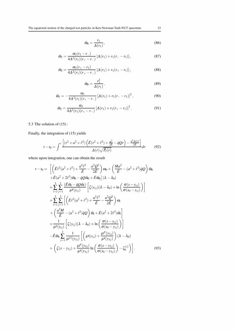
5.3 The solution of (15) :
Finally, the integration of (15) yields
t − t0 =∫ r
[
(r2 + a2 + ℓ2)(
E(r2 + ℓ2)+ a2
2E− qQr
)
− a2∆ (r)2E
]
∆(r)√
Pr(r)dr (92)
where upon integration, one can obtain the result
t − t0 =
[(
Eℓ2(a2 + ℓ2)+a2ℓ2
E− a2Q2
2E
)
ω0 +
(
Ma2
E− (a2 + ℓ2)qQ
)
ω0
+E(a2 + 2ℓ2)ω0 − qQω0 + Eω0
]
(λ −λ0)
+3
∑i=1
2
∑j=1
(Eωi − qQωi)
℘′(yi j)
[
ζ (yi j)(λ −λ0)+ ln
(
σ(s− yi j)
σ(s0 − yi j)
)]
+2
∑i=1
2
∑j=1
[(
Eℓ2(a2 + ℓ2)+a2ℓ2
E− a2Q2
2E
)
ωi
+
(
a2M
E− (a2 + ℓ2)qQ
)
ωi + E(a2 + 2ℓ2)ωi
]
× 1
℘′(yi j)
[
ζ (yi j)(λ −λ0)+ ln
(
σ(s− yi j)
σ(s0 − yi j)
)]
−Eω4
2
∑j=1
1
℘′2(y3 j)
[(
℘(y3 j)+℘′′(y3 j)
℘′(y3 j)
)
(λ −λ0)
+
(
ζ (s− y3 j)+℘′′(y3 j)
℘′(y3 j)ln
(
σ(s− y3 j)
σ(s0 − y3 j)
)
− ζ( j)0
)]
. (93)

24 Hakan Cebeci et al.
In addition, we identify℘(y3 j) = y3 =α212
( j = 1,2) with℘(y31) =℘(y32) = y3 =α212
.
We further calculate
ω0 =r3
1
∆(r1), (94)
ω1 =α3 [∆(r1)+ r1(r−− r1)]
3
4∆ 2(r1)(r+− r−)(r1 − r−), (95)
ω2 =α3 [∆(r1)+ r1(r+− r1)]
3
4∆ 2(r1)(r+− r−)(r+− r1), (96)
ω3 =α3∆(r1)
4(r1 − r−)(r1 − r+), (97)
ω0 =r4
1
∆(r1), (98)
ω1 =∆ 2(r1)r
41α2
2 [∆(r1)α2 + 3(r−− r1)α3]2 + 81 [∆(r1)+ (r−− r1)r1]
4 α43
324∆ 2(r1)(r−− r+)(r−− r1)2α33
, (99)
ω2 =∆ 2(r1)r
41α2
2 [∆(r1)α2 + 3(r+− r1)α3]2 + 81 [∆(r1)+ (r+− r1)r1]
4 α43
324∆ 2(r1)(r+− r−)(r+− r1)2α33
, (100)
ω3 =∆(r1)
[
r41α3
2 (∆(r1)(M− r1)α2 + 3(r−− r1)(r+− r1)α3)+ 81∆(r1)(r1 +M)α43
]
162(r1 − r−)2(r1 − r+)2α33
,
(101)
ω4 =∆(r1)
(
r41α4
2 + 81α43
)
1296(r1 − r−)(r1 − r+)α23
. (102)
Before closing this section, again we should point out that these solutions have been
obtained for non-zero NUT parameter where the relation (10) has been used as a
constraint between energy and angular momentum of test particle moving over the
equatorial plane of KNTN spacetime. To examine limiting cases, we note that when
ℓ= 0 (vanishing NUT parameter), the analytical solutions presented in [27] are recov-
ered provided that if one takes L = a(2E2−1)2E
for the angular momentum and Km2 =
a2
4E2
for Carter constant in the related paper (by taking θ = π2
and magnetic charge to be
zero as well in that work).
As a final remark, using analytical solutions presented above, we obtain trajectories of
charged test particle for bound and escape orbits over the equatorial plane for E2 > 1,
E2 < 1 and E2 = 1. These are illustrated in Figures 4-7.

The equatorial motion of the charged test particles in Kerr-Newman-Taub-NUT spacetime 25
(a)
(b) (c)
Fig. 4: Bound and escape orbits for E2 > 1 with parameters M = 1, a = 0.9, Q = 0.4,
ℓ= 0.05. Here, the roots of the radial potential P(r) satisfy r4 < 0 < r−e < r3 < r− <r+ < r2 < r+e < r1. Figure 4b illustrates the bound orbit in the ergoregion where
r+ < r < r2 < r+e for the test particle with q = −10 and E = −2. Here, the test
particle cannot exit from ergoregion. The dashed circles indicate the bounds of the
radial motion. Figure 4c illustrates the escape orbit in region where r > r1 for the test
particle with q = 10 and E = 2.
5.4 Calculation of the perihelion shift for a bound orbit
Here, to get an expression for the perihelion shift for a bound orbit, we consider that
the motion in the radial direction is bounded in the interval r2 ≤ r ≤ r1. Then, one
can evaluate the fundamental period Λr for the radial motion as
Λr = 2
∫ r1
r2
dr√
Pr(r)= 2
∫ ∞
y0
dy√
P3(y)(103)

26 Hakan Cebeci et al.
(a) (b)
Fig. 5: Bound orbit for E2 < 1 with parameters M = 1, a = 3.3, Q = 5 and ℓ = 5.94.
Here, the roots of the radial potential P(r) satisfy r4 < r−e < 0 < r− < r+ < r3 <r2 < r+e < r1. Figure 5b illustrates the bound orbit in the region where r2 < r < r1 for
the test particle with q = 5 and E = 0.9 (direct orbits with L > 0). The test particle
with positive energy enters into ergoregion and can exit from that region.The dashed
circles indicate the bounds of the radial motion. On the Pr(r) graph the smallest root
cannot be illustrated since r4 =−240.773 is out of the scale range of the radial coor-
dinate.
(a) (b)
Fig. 6: Bound orbit for E2 < 1 with parameters M = 1, a = 0.9, Q = 0.4 and ℓ= 0.1.
Here, the roots of the radial potential P(r) satisfy r4 < r3 < 0 < r−e < r2 < r− < r+ <r+e < r1. Figure 6b illustrates the bound orbit in the region where r+ < r < r1 for the
test particle with q = 18.74 and E = 0.073 (retrograde orbits with L < 0). Again the
test particle with positive energy enters into ergoregion and can exit from that region.
The dashed circles indicate the bounds of the radial motion.

The equatorial motion of the charged test particles in Kerr-Newman-Taub-NUT spacetime 27
(a) (b)
(c)
Fig. 7: Bound and escape orbits for E = 1 with parameters M = 1, a= 3.4, Q = 5 and
ℓ= 6. Here, the roots of the radial potential P(r) satisfy r−e < 0< r− < r+ < r3 < r2 <r+e < r1. Figure 7b illustrates the bound orbit in the region where r2 < r < r1 for the
test particle with q = 5. For the bound motion, test particle with positive unity energy
can enter into ergoregion where r+ < r+e and can exit from that region. The dashed
circles indicate the bounds of the radial motion. Figure 7c illustrates the crossover
escape orbit in region where −∞ < r < r− for the test particle with q = 5. Here the
test particle can enter into ergoregion where r−e < r− and can escape from that region
to negative infinity.
where P3(y) = 4y3 − g2y− g3 with g2 and g3 introduced in (77). The integral can be
calculated via the transformation
ξ =1
κ
(
y2 − y3
y− y3
)1/2
(104)
where y1, y2 and y3 correspond to the roots of the polynomial P3(y) = 0 (ordered
as y3 < y2 < y1) with κ2 = y2−y3y1−y3
. We also choose y0 = y1. Then one gets the radial
period as
Λr =2√
y1 − y3
K(κ) (105)
where K(κ) denotes the complete elliptic function with modulus κ . Then, one can
also evaluate the corresponding angular frequency
ϒr =2π
Λr
=π√
y1 − y3
K(κ)(106)
for the radial motion. Furthermore, one can obtain the angular frequencies ϒϕ and ϒt
for the ϕ-motion and t-motion respectively from the solutions of ϕ(λ ) and t(λ ). By

28 Hakan Cebeci et al.
using the arguments exposed in [50], one can notice that the solutions ϕ(λ ) and t(λ )can both be written in the forms
ϕ(λ ) =ϒϕ (λ −λ0)+ ϕ(λ ) (107)
and
t(λ ) =ϒt (λ −λ0)+ t(λ ), (108)
where ϒϕ and ϒt correspond to frequencies with respect to time parameter λ for ϕ-
motion and t-motion respectively. From these two solutions, one can get the corre-
sponding angular frequencies as
ϒϕ = a
[(
Eℓ2 +1
2E
(
ℓ2 −Q2)
)
ω0 +
(
M
E− qQ
)
ω0 +
(
2E2 − 1
2E
)
ω0
]
(109)
+ a2
∑i=1
2
∑j=1
[(
Eℓ2 +1
2E
(
ℓ2 −Q2)
)
ωi +
(
M
E− qQ
)
ωi +
(
2E2 − 1
2E
)
ωi
]
ζ (yi j)
℘′(yi j)
and
ϒt =
[(
Eℓ2(a2 + ℓ2)+a2ℓ2
E− a2Q2
2E
)
ω0 +
(
Ma2
E− (a2 + ℓ2)qQ
)
ω0
+E(a2 + 2ℓ2)ω0 − qQω0 + Eω0
]
+3
∑i=1
2
∑j=1
(Eωi − qQωi)
℘′(yi j)ζ (yi j)− Eω4
2
∑j=1
1
℘′2(y3 j)
(
℘(y3 j)+℘′′(y3 j)
℘′(y3 j)
)
+2
∑i=1
2
∑j=1
ζ (yi j)
℘′(yi j)
[(
Eℓ2(a2 + ℓ2)+a2ℓ2
E− a2Q2
2E
)
ωi
+
(
a2M
E− (a2 + ℓ2)qQ
)
ωi + E(a2 + 2ℓ2)ωi
]
. (110)
Finally, as is also outlined in [50], [51] and [52], the angular frequencies obtained
using the time parameter λ can be related to the angular frequencies Ωr and Ωϕ
obtained with respect to a distant observer time as
Ωr =ϒr
ϒt
, Ωϕ =ϒϕ
ϒt
. (111)
Obviously, these frequencies are not equal to each other. Therefore, it enables us to
calculate the perihelion shift in the form
Ωperihelion = Ωϕ −Ωr. (112)
It is clear that, the perihelion shift explicitly depends on the NUT parameter and other
physical spacetime parameters as well as the charge and the energy of the test par-
ticle. If one makes a comparison of this theoretical expression with those provided
in astronomical observations, one can possibly comment about the existence of the
NUT parameter in the real physical world [53]. Although we couldn’t provide a nu-
merical value for the perihelion precision, one can see that the NUT parameter and
the charge of the test particle have a definite influence on the perihelion shift.

The equatorial motion of the charged test particles in Kerr-Newman-Taub-NUT spacetime 29
6 Conclusion
In this study, we have comprehensively examined the equatorial orbits of a charged
test particle in the background of KNTN spacetime. Having obtained the governing
orbit equations, we have made an analysis of possible orbit types that would come
out via the analysis of radial potential Pr(r). We have accomplished a comprehensive
investigation of equatorial orbit types with respect to the value of the energy E of the
test particle and the form of the radial potential Pr(r). To see the effect of NUT pa-
rameter on the formation of possible orbit configurations, we have made a graphical
analysis with respect to change in NUT parameter. Next, by using Descartes’ rule of
sign, we have made a detailed investigation of the existence of bound orbits in the
causality-preserving region (outside the event horizon where r > r+) and obtained
required conditions for the existence (or non-existence) of them. In addition, we have
investigated the required conditions for the existence of equatorial circular orbits for
charged and uncharged particles. It is seen that the relations (52) and (53) determine
the existence of equatorial circular orbits for a charged test particle in KNTN space-
time while the expressions (57) and (58) fix the conditions for the existence of circular
orbits for an uncharged test particle.
As a further remark, we have worked out elliptical Newtonian orbits over equatorial
plane in presence of NUT charge. We have explicitly seen that unlike the other space-
time parameters (a, Q and M), the effect of the NUT parameter can be observed as the
general relativistic correction (improvement) to classical Newtonian orbits. Finally,
to obtain trajectory of charged test particle in equatorial KNTN spacetime, we have
solved orbit equations and obtained the exact analytical solutions in terms of Weier-
strass ℘, σ and ζ functions. Using these analytical solutions, we have also plotted
trajectories of charged test particle for bound and escape orbits in the regions where
r < r− and r > r+. In addition, as a physical observable, we have calculated the per-
ihelion shift for a bound orbit over the equatorial plane where it obviously depends
on the NUT and other physical parameters. We believe that, one can surely comment
on the existence of the NUT parameter in the universe if the theoretical expression
for the perihelion shift is compared with the numerical values provided through as-
tronomical observations. Also we can comment that a comprehensive investigation
of gravitational waves can lead to detection of NUT charge in the universe as well.
For a future study, it would also be physically interesting to investigate the equatorial
orbits of the charged test particles in rotating Taub-NUT spacetimes with cosmolog-
ical constant (Kerr-Newman-Taub-NUT-(A)dS spacetimes). In particular, the inves-
tigation of the existence of equatorial circular orbits in such a spacetime deserves
further study to see the effect of the cosmological constant. These are devoted to
future research.
Acknowledgements We would like to thank anonymous reviewers for their suggestions and comments.
References
1. E. Newman, L. Tamburino, T. Unti, Empty space generalization of the Schwarzschild metric, J. Math.
Phys. 4, 915 (1963).
30 Hakan Cebeci et al.
2. M. Demianski and E. T. Newman, A combined Kerr-NUT solution of the Einstein field equations,
Bull. Acad. Polon. Sci. Math. Astron. Phys. 14, 653 (1966).
3. C. W. Misner, The flatter regions of Newman, Unti and Tamburino’s generalized Schwarzschild
space, J. Math. Phys. 4, 924 (1963).
4. W. B. Bonnor, A new interpretation of the NUT metric in general relativity, Math. Proc. Camb. Phil.
Soc. 66, 145 (1969).
5. J. G. Miller, Global analysis of the Kerr-Taub-NUT metric, J. Math. Phys. 14, 486 (1973).
6. M. Nouri-Zonoz and D. Lynden-Bell, Gravitomagnetic lensing by NUT space, Mon. Not. Astron.
Soc. 292, 714 (1997).
7. D. Lynden-Bell, M. Nouri-Zonoz, Classical monopoles: Newton, NUT space, gravitomagnetic lens-
ing and atomic spectra, Rev. Mod. Phys. 70, 427 (1998).
8. D. Bini, C. Cherubini, R. T. Jantzen, On the interaction of massless fields with a gravitomagnetic
monopole, Class. Quant. Grav. 19, 5265 (2002).
9. D. Bini, C. Cherubini, R. T. Jantzen, B. Mashhoon, Gravitomagnetism in the Kerr-Newman-Taub-
NUT spacetime, Class. Quant. Grav. 20, 457 (2003).
10. A. N. Aliev, Rotating spacetimes with asymptotic non-flat structure and the gyromagnetic ratio ,
Phys. Rev. D 77, 044038 (2008).
11. G. D. Esmer, Separability and hidden symmetries of Kerr-Taub-NUT spacetime in Kaluza-Klein
theory , Grav. Cosmol. 19, 139 (2013).
12. C. Liu, S. Chen, C. Ding, J. Jing, Particle Acceleration on the Background of the Kerr-Taub-NUT
Spacetime, Phys. Lett. B 701, 285 (2011).
13. R. L. Zimmerman, B. Y. Shahir, Geodesics for the NUT metric and gravitational monopoles, Gen.
Relativ. Gravit. 21, 8, 821 (1989).
14. V. Kagramanova, J. Kunz, E. Hackmann and C. Lammerzahl, Analytic treatment of complete and
incomplete geodesics in Taub-NUT space-times, Phys. Rev. D 81, 124044 (2010).
15. A. A. Abdujabbarov, B. J. Ahmedov, V. G. Kagramanova, Particle motion and electromagnetic fields
of rotating compact gravitating objects with gravitomagnetic charge, Gen. Relativ. Gravit. 40, 2515
(2008).
16. A. A. Abdujabbarov, B. J. Ahmedov, S. R. Shaymatov, A. S. Rakhmatov, Penrose process in Kerr-
Taub-NUT spacetime, Astrophys. Space Sci. 334, 237 (2011).
17. A. Grenzebach, V. Perlick and C. Lammerzahl, Photon regions and shadows of Kerr-Newman-NUT
black holes with a cosmological constant, Phys. Rev. D 89, 124004 (2014).
18. Pradhan, P., Circular geodesics in the Kerr-Newman-Taub-NUT spacetime, Class. Quant. Grav. 32,
165001 (2015).
19. P. I. Jefremov and V. Perlick, Circular motion in NUT space-time, Class. Quant. Grav. 33, 245014
(2016).
20. G. Clement, M, Guenouche, Motion of charged particles in a NUTty Einstein-Maxwell spacetime
and causality violation, Gen. Rel. Grav. 50 60 (2018).
21. Mukharjee, S., Chakraborty, S., Dadhich, N., On some novel features of the Kerr-Newman-NUT
spacetime, Eur. Phys. J. C 79, 161 (2019).
22. B. P. Abbott et al. [LIGO Scientific and Virgo Collaborations], Observation of gravitational waves
from a binary black hole merger, Phys. Rev. Lett. 116, 061102 (2016).
23. S. Grunau, V. Kagramanova, Geodesics of electrically and magnetically charged test particles in the
Reissner-Nordstrom spacetime: Analytical solutions, Phys. Rev. D 83, 044009 (2011).
24. K. Flathmann, S. Grunau, Analytic solutions of the geodesic equation for Einstein-Maxwell-dilaton-
axion black holes, Phys. Rev. D 92, 104027 (2015).
25. D. Pugliese, H. Quevedo and R. Ruffini, Motion of charged test particles in Reissner-Nordstrom
spacetime, Phys. Rev. D 83, 104052 (2011).
26. M. Olivares, J. Saavedra, C. Leiva and J. Villanueva, Motion of charged particles on the Reissner-
Nordstrom (Anti)-de Sitter black holes, Mod. Phys. Lett. A 26, 2923 (2011).
27. E. Hackmann, H. Xu, Charged particle motion in Kerr-Newmann space-times, Phys. Rev. D 87,
124030 (2013).
28. S. Soroushfar, R. Saffari, S. Kazempour, S. Grunau and J. Kunz, Detailed study of geodesics in the
Kerr-Newman-(A)dS spacetime and the rotating charged black hole spacetime in f (R) gravity, Phys.
Rev. D 94, 024052 (2016).
29. H. Cebeci, N. Ozdemir, S. Sentorun, Motion of the charged test particles in Kerr-Newman-Taub-NUT
spacetime and analytical solutions, Phys. Rev. D 93, 104031 (2016).
30. J. M. Bardeen, W. H. Press and S. A. Teukolsky, Rotating black holes: Locally nonrotating frames,
energy extraction and scalar synchrotron radiation, Astrophys. J. 178, 347 (1972).

The equatorial motion of the charged test particles in Kerr-Newman-Taub-NUT spacetime 31
31. N. Dadhich and P. P. Kale, Equatorial circular geodesics in the Kerr-Newman geometry, J. Math.
Phys. 18, 1727 (1977).
32. D. Pugliese, H. Quevedo and R. Ruffini, Equatorial circular orbits of neutral test particles in the
Kerr-Newman spacetime, Phys. Rev. D 88, 024042 (2013).
33. Z. Stuchlık and P. Slany, Equatorial circular orbits in the Kerr-de Sitter spacetimes, Phys. Rev. D
69, 064001 (2004).
34. P. Slany, M. Pokorna, Z. Stuchlık , Equatorial circular orbits in Kerr-anti-de Sitter spacetimes, Gen.
Rel. Grav. 45, 2611 (2013).
35. R. M. Wald, General Relativity (Chicago: The University of Chicago Press) (1984).
36. S. Chandrasekhar, The Mathematical Theory of Black Holes (London: Clarendon Press) (1983).
37. B. Carter, Hamilton-Jacobi and Schrodinger separable solutions of Einstein’s equations ,Commun.
Math. Phys. 10, 280 (1968).
38. B. Carter, Phys. Rev.,Global structure of the Kerr family of gravitational fields, 174, 1559 (1968).
39. R. Debever, N. Kamran and R. G. Mc Lenaghan, Exhaustive integration and a single expression for
the general solution of the type D vacuum and electrovac field equations with cosmological constant
for a nonsingular aligned Maxwell field, J. Math. Phys. 25, 1955 (1984).
40. V. P. Frolov, P. Krtous, and D. Kubiznak, Separability of Hamilton-Jacobi and Klein-Gordon equa-
tions in general Kerr-NUT-AdS spacetimes, J. High Energy Phys. 02, 005 (2007).
41. A. F. Zakharov, On the hotspot near a Kerr black hole: Monte Carlo simulations, Mon. Not. R.
Astron. Soc. 269, 283 (1994).
42. Y. Mino, Perturbative approach to an orbital evolution around a supermassive black hole, Phys.
Rev. D 67, 084027 (2003).
43. D. Pugliese , H. Quevedo, The ergoregion in the Kerr spacetime : properties of the equatorial circu-
lar motion, Eur. Phys. J. C 75, 234 (2015).
44. D. Pugliese, H. Quevedo, Observers in Kerr spacetimes , Eur. Phys. J. C 78, 69 (2018).
45. B. O’Neill, The Geometry of Kerr Black Holes (Massachusetts: A K Peters/CRC Press) (1995).
46. D. C. Wilkins, Bound geodesics in the Kerr metric, Phys. Rev. D 5, 814 (1972).
47. T. Dereli, R. W. Tucker, On the detection of scalar field induced space-time torsion, Mod. Phys. Lett.
A 17, 421 (2002).
48. H. Cebeci, T. Dereli, R. W. Tucker, Autoparallel orbits in Kerr Brans-Dicke spacetimes, International
Journal of Modern Physics D 13, 137 (2004).
49. Z. X. Wang, D. R. Guo, Special Functions, (Singapore: World Scientific Publishing Co.) (1989).
50. S. Drasco, S. A. Hughes, Rotating black hole orbit functionals in the frequency domain, Phys. Rev.
D 69, 044015 (2004).
51. R. Fujita, W. Hikida, Analytical Solutions of bound timelike geodesic orbits in Kerr spacetime, Class.
Quant. Grav. 26, 135002 (2009).
52. E. Hackmann and C. Lammerzahl, Observables for bound orbital motion in axially symmetric space-
times, Phys. Rev. D 85, 044049 (2012).
53. C. Chakraborty and S. Bhattacharyya, Does the gravitomagnetic monopole exist? A clue from a black
hole x-ray binary, , Phys. Rev. D 98, 043021 (2018).