SECOND EDITION

Hadoop: The Definitive Guide

Tom Whiteforeword by Doug Cutting

Beijing • Cambridge • Farnham • Köln • Sebastopol • Tokyo

Hadoop: The Definitive Guide, Second Editionby Tom White

Copyright © 2011 Tom White. All rights reserved.Printed in the United States of America.

Published by O’Reilly Media, Inc., 1005 Gravenstein Highway North, Sebastopol, CA 95472.

O’Reilly books may be purchased for educational, business, or sales promotional use. Online editionsare also available for most titles (http://my.safaribooksonline.com). For more information, contact ourcorporate/institutional sales department: (800) 998-9938 or corporate@oreilly.com.

Editor: Mike LoukidesProduction Editor: Adam ZarembaProofreader: Diane Il Grande

Indexer: Jay Book ServicesCover Designer: Karen MontgomeryInterior Designer: David FutatoIllustrator: Robert Romano

Printing History:June 2009: First Edition. October 2010: Second Edition.

Nutshell Handbook, the Nutshell Handbook logo, and the O’Reilly logo are registered trademarks ofO’Reilly Media, Inc. Hadoop: The Definitive Guide, the image of an African elephant, and related tradedress are trademarks of O’Reilly Media, Inc.

Many of the designations used by manufacturers and sellers to distinguish their products are claimed astrademarks. Where those designations appear in this book, and O’Reilly Media, Inc. was aware of atrademark claim, the designations have been printed in caps or initial caps.

While every precaution has been taken in the preparation of this book, the publisher and author assumeno responsibility for errors or omissions, or for damages resulting from the use of the information con-tained herein.

ISBN: 978-1-449-38973-4

[SB]

1285179414

For Eliane, Emilia, and Lottie

Table of Contents

Foreword . . . . . . . . . . . . . . . . . . . . . . . . . . . . . . . . . . . . . . . . . . . . . . . . . . . . . . . . . . . . . . . . . . . xv

Preface . . . . . . . . . . . . . . . . . . . . . . . . . . . . . . . . . . . . . . . . . . . . . . . . . . . . . . . . . . . . . . . . . . . . xvii

1. Meet Hadoop . . . . . . . . . . . . . . . . . . . . . . . . . . . . . . . . . . . . . . . . . . . . . . . . . . . . . . . . . . . 1Data! 1Data Storage and Analysis 3Comparison with Other Systems 4

RDBMS 4Grid Computing 6Volunteer Computing 8

A Brief History of Hadoop 9Apache Hadoop and the Hadoop Ecosystem 12

2. MapReduce . . . . . . . . . . . . . . . . . . . . . . . . . . . . . . . . . . . . . . . . . . . . . . . . . . . . . . . . . . . 15A Weather Dataset 15

Data Format 15Analyzing the Data with Unix Tools 17Analyzing the Data with Hadoop 18

Map and Reduce 18Java MapReduce 20

Scaling Out 27Data Flow 28Combiner Functions 30Running a Distributed MapReduce Job 33

Hadoop Streaming 33Ruby 33Python 36

Hadoop Pipes 37Compiling and Running 38

v

3. The Hadoop Distributed Filesystem . . . . . . . . . . . . . . . . . . . . . . . . . . . . . . . . . . . . . . . 41The Design of HDFS 41HDFS Concepts 43

Blocks 43Namenodes and Datanodes 44

The Command-Line Interface 45Basic Filesystem Operations 46

Hadoop Filesystems 47Interfaces 49

The Java Interface 51Reading Data from a Hadoop URL 51Reading Data Using the FileSystem API 52Writing Data 55Directories 57Querying the Filesystem 57Deleting Data 62

Data Flow 62Anatomy of a File Read 62Anatomy of a File Write 65Coherency Model 68

Parallel Copying with distcp 70Keeping an HDFS Cluster Balanced 71

Hadoop Archives 71Using Hadoop Archives 72Limitations 73

4. Hadoop I/O . . . . . . . . . . . . . . . . . . . . . . . . . . . . . . . . . . . . . . . . . . . . . . . . . . . . . . . . . . . 75Data Integrity 75

Data Integrity in HDFS 75LocalFileSystem 76ChecksumFileSystem 77

Compression 77Codecs 78Compression and Input Splits 83Using Compression in MapReduce 84

Serialization 86The Writable Interface 87Writable Classes 89Implementing a Custom Writable 96Serialization Frameworks 101Avro 103

File-Based Data Structures 116SequenceFile 116

vi | Table of Contents

MapFile 123

5. Developing a MapReduce Application . . . . . . . . . . . . . . . . . . . . . . . . . . . . . . . . . . . . 129The Configuration API 130

Combining Resources 131Variable Expansion 132

Configuring the Development Environment 132Managing Configuration 132GenericOptionsParser, Tool, and ToolRunner 135

Writing a Unit Test 138Mapper 138Reducer 140

Running Locally on Test Data 141Running a Job in a Local Job Runner 141Testing the Driver 145

Running on a Cluster 146Packaging 146Launching a Job 146The MapReduce Web UI 148Retrieving the Results 151Debugging a Job 153Using a Remote Debugger 158

Tuning a Job 160Profiling Tasks 160

MapReduce Workflows 163Decomposing a Problem into MapReduce Jobs 163Running Dependent Jobs 165

6. How MapReduce Works . . . . . . . . . . . . . . . . . . . . . . . . . . . . . . . . . . . . . . . . . . . . . . . . 167Anatomy of a MapReduce Job Run 167

Job Submission 167Job Initialization 169Task Assignment 169Task Execution 170Progress and Status Updates 170Job Completion 172

Failures 173Task Failure 173Tasktracker Failure 175Jobtracker Failure 175

Job Scheduling 175The Fair Scheduler 176The Capacity Scheduler 177

Table of Contents | vii

Shuffle and Sort 177The Map Side 177The Reduce Side 179Configuration Tuning 180

Task Execution 183Speculative Execution 183Task JVM Reuse 184Skipping Bad Records 185The Task Execution Environment 186

7. MapReduce Types and Formats . . . . . . . . . . . . . . . . . . . . . . . . . . . . . . . . . . . . . . . . . . 189MapReduce Types 189

The Default MapReduce Job 191Input Formats 198

Input Splits and Records 198Text Input 209Binary Input 213Multiple Inputs 214Database Input (and Output) 215

Output Formats 215Text Output 216Binary Output 216Multiple Outputs 217Lazy Output 224Database Output 224

8. MapReduce Features . . . . . . . . . . . . . . . . . . . . . . . . . . . . . . . . . . . . . . . . . . . . . . . . . . 225Counters 225

Built-in Counters 225User-Defined Java Counters 227User-Defined Streaming Counters 232

Sorting 232Preparation 232Partial Sort 233Total Sort 237Secondary Sort 241

Joins 247Map-Side Joins 247Reduce-Side Joins 249

Side Data Distribution 252Using the Job Configuration 252Distributed Cache 253

MapReduce Library Classes 257

viii | Table of Contents

9. Setting Up a Hadoop Cluster . . . . . . . . . . . . . . . . . . . . . . . . . . . . . . . . . . . . . . . . . . . . 259Cluster Specification 259

Network Topology 261Cluster Setup and Installation 263

Installing Java 264Creating a Hadoop User 264Installing Hadoop 264Testing the Installation 265

SSH Configuration 265Hadoop Configuration 266

Configuration Management 267Environment Settings 269Important Hadoop Daemon Properties 273Hadoop Daemon Addresses and Ports 278Other Hadoop Properties 279User Account Creation 280

Security 281Kerberos and Hadoop 282Delegation Tokens 284Other Security Enhancements 285

Benchmarking a Hadoop Cluster 286Hadoop Benchmarks 287User Jobs 289

Hadoop in the Cloud 289Hadoop on Amazon EC2 290

10. Administering Hadoop . . . . . . . . . . . . . . . . . . . . . . . . . . . . . . . . . . . . . . . . . . . . . . . . . 293HDFS 293

Persistent Data Structures 293Safe Mode 298Audit Logging 300Tools 300

Monitoring 305Logging 305Metrics 306Java Management Extensions 309

Maintenance 312Routine Administration Procedures 312Commissioning and Decommissioning Nodes 313Upgrades 316

11. Pig . . . . . . . . . . . . . . . . . . . . . . . . . . . . . . . . . . . . . . . . . . . . . . . . . . . . . . . . . . . . . . . . . 321Installing and Running Pig 322

Table of Contents | ix

Execution Types 322Running Pig Programs 324Grunt 324Pig Latin Editors 325

An Example 325Generating Examples 327

Comparison with Databases 328Pig Latin 330

Structure 330Statements 331Expressions 335Types 336Schemas 338Functions 342

User-Defined Functions 343A Filter UDF 343An Eval UDF 347A Load UDF 348

Data Processing Operators 351Loading and Storing Data 351Filtering Data 352Grouping and Joining Data 354Sorting Data 359Combining and Splitting Data 360

Pig in Practice 361Parallelism 361Parameter Substitution 362

12. Hive . . . . . . . . . . . . . . . . . . . . . . . . . . . . . . . . . . . . . . . . . . . . . . . . . . . . . . . . . . . . . . . . 365Installing Hive 366

The Hive Shell 367An Example 368Running Hive 369

Configuring Hive 369Hive Services 371The Metastore 373

Comparison with Traditional Databases 375Schema on Read Versus Schema on Write 376Updates, Transactions, and Indexes 376

HiveQL 377Data Types 378Operators and Functions 380

Tables 381

x | Table of Contents

Managed Tables and External Tables 381Partitions and Buckets 383Storage Formats 387Importing Data 392Altering Tables 394Dropping Tables 395

Querying Data 395Sorting and Aggregating 395MapReduce Scripts 396Joins 397Subqueries 400Views 401

User-Defined Functions 402Writing a UDF 403Writing a UDAF 405

13. HBase . . . . . . . . . . . . . . . . . . . . . . . . . . . . . . . . . . . . . . . . . . . . . . . . . . . . . . . . . . . . . . . 411HBasics 411

Backdrop 412Concepts 412

Whirlwind Tour of the Data Model 412Implementation 413

Installation 416Test Drive 417

Clients 419Java 419Avro, REST, and Thrift 422

Example 423Schemas 424Loading Data 425Web Queries 428

HBase Versus RDBMS 431Successful Service 432HBase 433Use Case: HBase at Streamy.com 433

Praxis 435Versions 435HDFS 436UI 437Metrics 437Schema Design 438Counters 438Bulk Load 439

Table of Contents | xi

14. ZooKeeper . . . . . . . . . . . . . . . . . . . . . . . . . . . . . . . . . . . . . . . . . . . . . . . . . . . . . . . . . . . 441Installing and Running ZooKeeper 442An Example 443

Group Membership in ZooKeeper 444Creating the Group 444Joining a Group 447Listing Members in a Group 448Deleting a Group 450

The ZooKeeper Service 451Data Model 451Operations 453Implementation 457Consistency 458Sessions 460States 462

Building Applications with ZooKeeper 463A Configuration Service 463The Resilient ZooKeeper Application 466A Lock Service 470More Distributed Data Structures and Protocols 472

ZooKeeper in Production 473Resilience and Performance 473Configuration 474

15. Sqoop . . . . . . . . . . . . . . . . . . . . . . . . . . . . . . . . . . . . . . . . . . . . . . . . . . . . . . . . . . . . . . . 477Getting Sqoop 477A Sample Import 479Generated Code 482

Additional Serialization Systems 482Database Imports: A Deeper Look 483

Controlling the Import 485Imports and Consistency 485Direct-mode Imports 485

Working with Imported Data 486Imported Data and Hive 487

Importing Large Objects 489Performing an Export 491Exports: A Deeper Look 493

Exports and Transactionality 494Exports and SequenceFiles 494

16. Case Studies . . . . . . . . . . . . . . . . . . . . . . . . . . . . . . . . . . . . . . . . . . . . . . . . . . . . . . . . . 497Hadoop Usage at Last.fm 497

xii | Table of Contents

Last.fm: The Social Music Revolution 497Hadoop at Last.fm 497Generating Charts with Hadoop 498The Track Statistics Program 499Summary 506

Hadoop and Hive at Facebook 506Introduction 506Hadoop at Facebook 506Hypothetical Use Case Studies 509Hive 512Problems and Future Work 516

Nutch Search Engine 517Background 517Data Structures 518Selected Examples of Hadoop Data Processing in Nutch 521Summary 530

Log Processing at Rackspace 531Requirements/The Problem 531Brief History 532Choosing Hadoop 532Collection and Storage 532MapReduce for Logs 533

Cascading 539Fields, Tuples, and Pipes 540Operations 542Taps, Schemes, and Flows 544Cascading in Practice 545Flexibility 548Hadoop and Cascading at ShareThis 549Summary 552

TeraByte Sort on Apache Hadoop 553Using Pig and Wukong to Explore Billion-edge Network Graphs 556

Measuring Community 558Everybody’s Talkin’ at Me: The Twitter Reply Graph 558Symmetric Links 561Community Extraction 562

A. Installing Apache Hadoop . . . . . . . . . . . . . . . . . . . . . . . . . . . . . . . . . . . . . . . . . . . . . . 565

B. Cloudera’s Distribution for Hadoop . . . . . . . . . . . . . . . . . . . . . . . . . . . . . . . . . . . . . . 571

C. Preparing the NCDC Weather Data . . . . . . . . . . . . . . . . . . . . . . . . . . . . . . . . . . . . . . . 573

Table of Contents | xiii

Index . . . . . . . . . . . . . . . . . . . . . . . . . . . . . . . . . . . . . . . . . . . . . . . . . . . . . . . . . . . . . . . . . . . . . 577

xiv | Table of Contents

Foreword

Hadoop got its start in Nutch. A few of us were attempting to build an open sourceweb search engine and having trouble managing computations running on even ahandful of computers. Once Google published its GFS and MapReduce papers, theroute became clear. They’d devised systems to solve precisely the problems we werehaving with Nutch. So we started, two of us, half-time, to try to re-create these systemsas a part of Nutch.

We managed to get Nutch limping along on 20 machines, but it soon became clear thatto handle the Web’s massive scale, we’d need to run it on thousands of machines and,moreover, that the job was bigger than two half-time developers could handle.

Around that time, Yahoo! got interested, and quickly put together a team that I joined.We split off the distributed computing part of Nutch, naming it Hadoop. With the helpof Yahoo!, Hadoop soon grew into a technology that could truly scale to the Web.

In 2006, Tom White started contributing to Hadoop. I already knew Tom through anexcellent article he’d written about Nutch, so I knew he could present complex ideasin clear prose. I soon learned that he could also develop software that was as pleasantto read as his prose.

From the beginning, Tom’s contributions to Hadoop showed his concern for users andfor the project. Unlike most open source contributors, Tom is not primarily interestedin tweaking the system to better meet his own needs, but rather in making it easier foranyone to use.

Initially, Tom specialized in making Hadoop run well on Amazon’s EC2 and S3 serv-ices. Then he moved on to tackle a wide variety of problems, including improving theMapReduce APIs, enhancing the website, and devising an object serialization frame-work. In all cases, Tom presented his ideas precisely. In short order, Tom earned therole of Hadoop committer and soon thereafter became a member of the Hadoop ProjectManagement Committee.

Tom is now a respected senior member of the Hadoop developer community. Thoughhe’s an expert in many technical corners of the project, his specialty is making Hadoopeasier to use and understand.

xv

Given this, I was very pleased when I learned that Tom intended to write a book aboutHadoop. Who could be better qualified? Now you have the opportunity to learn aboutHadoop from a master—not only of the technology, but also of common sense andplain talk.

—Doug CuttingShed in the Yard, California

xvi | Foreword

Preface

Martin Gardner, the mathematics and science writer, once said in an interview:

Beyond calculus, I am lost. That was the secret of my column’s success. It took me solong to understand what I was writing about that I knew how to write in a way mostreaders would understand.*

In many ways, this is how I feel about Hadoop. Its inner workings are complex, restingas they do on a mixture of distributed systems theory, practical engineering, and com-mon sense. And to the uninitiated, Hadoop can appear alien.

But it doesn’t need to be like this. Stripped to its core, the tools that Hadoop providesfor building distributed systems—for data storage, data analysis, and coordination—are simple. If there’s a common theme, it is about raising the level of abstraction—tocreate building blocks for programmers who just happen to have lots of data to store,or lots of data to analyze, or lots of machines to coordinate, and who don’t have thetime, the skill, or the inclination to become distributed systems experts to build theinfrastructure to handle it.

With such a simple and generally applicable feature set, it seemed obvious to me whenI started using it that Hadoop deserved to be widely used. However, at the time (inearly 2006), setting up, configuring, and writing programs to use Hadoop was an art.Things have certainly improved since then: there is more documentation, there aremore examples, and there are thriving mailing lists to go to when you have questions.And yet the biggest hurdle for newcomers is understanding what this technology iscapable of, where it excels, and how to use it. That is why I wrote this book.

The Apache Hadoop community has come a long way. Over the course of three years,the Hadoop project has blossomed and spun off half a dozen subprojects. In this time,the software has made great leaps in performance, reliability, scalability, and manage-ability. To gain even wider adoption, however, I believe we need to make Hadoop eveneasier to use. This will involve writing more tools; integrating with more systems; and

* “The science of fun,” Alex Bellos, The Guardian, May 31, 2008, http://www.guardian.co.uk/science/2008/may/31/maths.science.

xvii

writing new, improved APIs. I’m looking forward to being a part of this, and I hopethis book will encourage and enable others to do so, too.

Administrative NotesDuring discussion of a particular Java class in the text, I often omit its package name,to reduce clutter. If you need to know which package a class is in, you can easily lookit up in Hadoop’s Java API documentation for the relevant subproject, linked to fromthe Apache Hadoop home page at http://hadoop.apache.org/. Or if you’re using an IDE,it can help using its auto-complete mechanism.

Similarly, although it deviates from usual style guidelines, program listings that importmultiple classes from the same package may use the asterisk wildcard character to savespace (for example: import org.apache.hadoop.io.*).

The sample programs in this book are available for download from the website thataccompanies this book: http://www.hadoopbook.com/. You will also find instructionsthere for obtaining the datasets that are used in examples throughout the book, as wellas further notes for running the programs in the book, and links to updates, additionalresources, and my blog.

What’s in This Book?The rest of this book is organized as follows. Chapter 1 emphasizes the need for Hadoopand sketches the history of the project. Chapter 2 provides an introduction toMapReduce. Chapter 3 looks at Hadoop filesystems, and in particular HDFS, in depth.Chapter 4 covers the fundamentals of I/O in Hadoop: data integrity, compression,serialization, and file-based data structures.

The next four chapters cover MapReduce in depth. Chapter 5 goes through the practicalsteps needed to develop a MapReduce application. Chapter 6 looks at how MapReduceis implemented in Hadoop, from the point of view of a user. Chapter 7 is about theMapReduce programming model, and the various data formats that MapReduce canwork with. Chapter 8 is on advanced MapReduce topics, including sorting and joiningdata.

Chapters 9 and 10 are for Hadoop administrators, and describe how to set up andmaintain a Hadoop cluster running HDFS and MapReduce.

Later chapters are dedicated to projects that build on Hadoop or are related to it.Chapters 11 and 12 present Pig and Hive, which are analytics platforms built on HDFSand MapReduce, whereas Chapters 13, 14, and 15 cover HBase, ZooKeeper, andSqoop, respectively.

Finally, Chapter 16 is a collection of case studies contributed by members of the ApacheHadoop community.

xviii | Preface

What’s New in the Second Edition?The second edition has two new chapters on Hive and Sqoop (Chapters 12 and 15), anew section covering Avro (in Chapter 4), an introduction to the new security featuresin Hadoop (in Chapter 9), and a new case study on analyzing massive network graphsusing Hadoop (in Chapter 16).

This edition continues to describe the 0.20 release series of Apache Hadoop, since thiswas the latest stable release at the time of writing. New features from later releases areoccasionally mentioned in the text, however, with reference to the version that theywere introduced in.

Conventions Used in This BookThe following typographical conventions are used in this book:

ItalicIndicates new terms, URLs, email addresses, filenames, and file extensions.

Constant widthUsed for program listings, as well as within paragraphs to refer to program elementssuch as variable or function names, databases, data types, environment variables,statements, and keywords.

Constant width boldShows commands or other text that should be typed literally by the user.

Constant width italicShows text that should be replaced with user-supplied values or by values deter-mined by context.

This icon signifies a tip, suggestion, or general note.

This icon indicates a warning or caution.

Using Code ExamplesThis book is here to help you get your job done. In general, you may use the code inthis book in your programs and documentation. You do not need to contact us forpermission unless you’re reproducing a significant portion of the code. For example,writing a program that uses several chunks of code from this book does not requirepermission. Selling or distributing a CD-ROM of examples from O’Reilly books does

Preface | xix

require permission. Answering a question by citing this book and quoting examplecode does not require permission. Incorporating a significant amount of example codefrom this book into your product’s documentation does require permission.

We appreciate, but do not require, attribution. An attribution usually includes the title,author, publisher, and ISBN. For example: “Hadoop: The Definitive Guide, SecondEdition, by Tom White. Copyright 2011 Tom White, 978-1-449-38973-4.”

If you feel your use of code examples falls outside fair use or the permission given above,feel free to contact us at permissions@oreilly.com.

Safari® Books OnlineSafari Books Online is an on-demand digital library that lets you easilysearch over 7,500 technology and creative reference books and videos tofind the answers you need quickly.

With a subscription, you can read any page and watch any video from our library online.Read books on your cell phone and mobile devices. Access new titles before they areavailable for print, and get exclusive access to manuscripts in development and postfeedback for the authors. Copy and paste code samples, organize your favorites, down-load chapters, bookmark key sections, create notes, print out pages, and benefit fromtons of other time-saving features.

O’Reilly Media has uploaded this book to the Safari Books Online service. To have fulldigital access to this book and others on similar topics from O’Reilly and other pub-lishers, sign up for free at http://my.safaribooksonline.com.

How to Contact UsPlease address comments and questions concerning this book to the publisher:

O’Reilly Media, Inc.1005 Gravenstein Highway NorthSebastopol, CA 95472800-998-9938 (in the United States or Canada)707-829-0515 (international or local)707-829-0104 (fax)

We have a web page for this book, where we list errata, examples, and any additionalinformation. You can access this page at:

http://oreilly.com/catalog/0636920010388/

The author also has a site for this book at:

http://www.hadoopbook.com/

xx | Preface

To comment or ask technical questions about this book, send email to:

bookquestions@oreilly.com

For more information about our books, conferences, Resource Centers, and theO’Reilly Network, see our website at:

http://www.oreilly.com

AcknowledgmentsI have relied on many people, both directly and indirectly, in writing this book. I wouldlike to thank the Hadoop community, from whom I have learned, and continue to learn,a great deal.

In particular, I would like to thank Michael Stack and Jonathan Gray for writing thechapter on HBase. Also thanks go to Adrian Woodhead, Marc de Palol, Joydeep SenSarma, Ashish Thusoo, Andrzej Białecki, Stu Hood, Chris K. Wensel, and OwenO’Malley for contributing case studies for Chapter 16.

I would like to thank the following reviewers who contributed many helpful suggestionsand improvements to my drafts: Raghu Angadi, Matt Biddulph, Christophe Bisciglia,Ryan Cox, Devaraj Das, Alex Dorman, Chris Douglas, Alan Gates, Lars George, PatrickHunt, Aaron Kimball, Peter Krey, Hairong Kuang, Simon Maxen, Olga Natkovich,Benjamin Reed, Konstantin Shvachko, Allen Wittenauer, Matei Zaharia, and PhilipZeyliger. Ajay Anand kept the review process flowing smoothly. Philip (“flip”) Kromerkindly helped me with the NCDC weather dataset featured in the examples in this book.Special thanks to Owen O’Malley and Arun C. Murthy for explaining the intricacies ofthe MapReduce shuffle to me. Any errors that remain are, of course, to be laid at mydoor.

For the second edition, I owe a debt of gratitude for the detailed review and feedbackfrom Jeff Bean, Doug Cutting, Glynn Durham, Alan Gates, Jeff Hammerbacher, AlexKozlov, Ken Krugler, Jimmy Lin, Todd Lipcon, Sarah Sproehnle, Vinithra Varadhara-jan, and Ian Wrigley, as well as all the readers who submitted errata for the first edition.I would also like to thank Aaron Kimball for contributing the chapter on Sqoop, andPhilip (“flip”) Kromer for the case study on graph processing.

I am particularly grateful to Doug Cutting for his encouragement, support, and friend-ship, and for contributing the foreword.

Thanks also go to the many others with whom I have had conversations or emaildiscussions over the course of writing the book.

Halfway through writing this book, I joined Cloudera, and I want to thank mycolleagues for being incredibly supportive in allowing me the time to write, and to getit finished promptly.

Preface | xxi

I am grateful to my editor, Mike Loukides, and his colleagues at O’Reilly for their helpin the preparation of this book. Mike has been there throughout to answer my ques-tions, to read my first drafts, and to keep me on schedule.

Finally, the writing of this book has been a great deal of work, and I couldn’t have doneit without the constant support of my family. My wife, Eliane, not only kept the homegoing, but also stepped in to help review, edit, and chase case studies. My daughters,Emilia and Lottie, have been very understanding, and I’m looking forward to spendinglots more time with all of them.

xxii | Preface

CHAPTER 1

Meet Hadoop

In pioneer days they used oxen for heavy pulling, and when one ox couldn’t budge a log,they didn’t try to grow a larger ox. We shouldn’t be trying for bigger computers, but formore systems of computers.

—Grace Hopper

Data!We live in the data age. It’s not easy to measure the total volume of data stored elec-tronically, but an IDC estimate put the size of the “digital universe” at 0.18 zettabytesin 2006, and is forecasting a tenfold growth by 2011 to 1.8 zettabytes.* A zettabyte is1021 bytes, or equivalently one thousand exabytes, one million petabytes, or one billionterabytes. That’s roughly the same order of magnitude as one disk drive for every personin the world.

This flood of data is coming from many sources. Consider the following:†

• The New York Stock Exchange generates about one terabyte of new trade data perday.

• Facebook hosts approximately 10 billion photos, taking up one petabyte of storage.

• Ancestry.com, the genealogy site, stores around 2.5 petabytes of data.

• The Internet Archive stores around 2 petabytes of data, and is growing at a rate of20 terabytes per month.

• The Large Hadron Collider near Geneva, Switzerland, will produce about 15petabytes of data per year.

* From Gantz et al., “The Diverse and Exploding Digital Universe,” March 2008 (http://www.emc.com/collateral/analyst-reports/diverse-exploding-digital-universe.pdf).

† http://www.intelligententerprise.com/showArticle.jhtml?articleID=207800705, http://mashable.com/2008/10/15/facebook-10-billion-photos/, http://blog.familytreemagazine.com/insider/Inside+Ancestrycoms+TopSecret+Data+Center.aspx, and http://www.archive.org/about/faqs.php, http://www.interactions.org/cms/?pid=1027032.

1

So there’s a lot of data out there. But you are probably wondering how it affects you.Most of the data is locked up in the largest web properties (like search engines), orscientific or financial institutions, isn’t it? Does the advent of “Big Data,” as it is beingcalled, affect smaller organizations or individuals?

I argue that it does. Take photos, for example. My wife’s grandfather was an avidphotographer, and took photographs throughout his adult life. His entire corpus ofmedium format, slide, and 35mm film, when scanned in at high-resolution, occupiesaround 10 gigabytes. Compare this to the digital photos that my family took in 2008,which take up about 5 gigabytes of space. My family is producing photographic dataat 35 times the rate my wife’s grandfather’s did, and the rate is increasing every year asit becomes easier to take more and more photos.

More generally, the digital streams that individuals are producing are growing apace.Microsoft Research’s MyLifeBits project gives a glimpse of archiving of personal infor-mation that may become commonplace in the near future. MyLifeBits was an experi-ment where an individual’s interactions—phone calls, emails, documents—were cap-tured electronically and stored for later access. The data gathered included a phototaken every minute, which resulted in an overall data volume of one gigabyte a month.When storage costs come down enough to make it feasible to store continuous audioand video, the data volume for a future MyLifeBits service will be many times that.

The trend is for every individual’s data footprint to grow, but perhaps more important,the amount of data generated by machines will be even greater than that generated bypeople. Machine logs, RFID readers, sensor networks, vehicle GPS traces, retailtransactions—all of these contribute to the growing mountain of data.

The volume of data being made publicly available increases every year, too. Organiza-tions no longer have to merely manage their own data: success in the future will bedictated to a large extent by their ability to extract value from other organizations’ data.

Initiatives such as Public Data Sets on Amazon Web Services, Infochimps.org, and theinfo.org exist to foster the “information commons,” where data can be freely (or inthe case of AWS, for a modest price) shared for anyone to download and analyze.Mashups between different information sources make for unexpected and hithertounimaginable applications.

Take, for example, the Astrometry.net project, which watches the Astrometry groupon Flickr for new photos of the night sky. It analyzes each image and identifies whichpart of the sky it is from, as well as any interesting celestial bodies, such as stars orgalaxies. This project shows the kind of things that are possible when data (in this case,tagged photographic images) is made available and used for something (image analysis)that was not anticipated by the creator.

It has been said that “More data usually beats better algorithms,” which is to say thatfor some problems (such as recommending movies or music based on past preferences),

2 | Chapter 1: Meet Hadoop

however fiendish your algorithms are, they can often be beaten simply by having moredata (and a less sophisticated algorithm).‡

The good news is that Big Data is here. The bad news is that we are struggling to storeand analyze it.

Data Storage and AnalysisThe problem is simple: while the storage capacities of hard drives have increased mas-sively over the years, access speeds—the rate at which data can be read from drives—have not kept up. One typical drive from 1990 could store 1,370 MB of data and hada transfer speed of 4.4 MB/s,§ so you could read all the data from a full drive in aroundfive minutes. Over 20 years later, one terabyte drives are the norm, but the transferspeed is around 100 MB/s, so it takes more than two and a half hours to read all thedata off the disk.

This is a long time to read all data on a single drive—and writing is even slower. Theobvious way to reduce the time is to read from multiple disks at once. Imagine if wehad 100 drives, each holding one hundredth of the data. Working in parallel, we couldread the data in under two minutes.

Only using one hundredth of a disk may seem wasteful. But we can store one hundreddatasets, each of which is one terabyte, and provide shared access to them. We canimagine that the users of such a system would be happy to share access in return forshorter analysis times, and, statistically, that their analysis jobs would be likely to bespread over time, so they wouldn’t interfere with each other too much.

There’s more to being able to read and write data in parallel to or from multiple disks,though.

The first problem to solve is hardware failure: as soon as you start using many piecesof hardware, the chance that one will fail is fairly high. A common way of avoiding dataloss is through replication: redundant copies of the data are kept by the system so thatin the event of failure, there is another copy available. This is how RAID works, forinstance, although Hadoop’s filesystem, the Hadoop Distributed Filesystem (HDFS),takes a slightly different approach, as you shall see later.

The second problem is that most analysis tasks need to be able to combine the data insome way; data read from one disk may need to be combined with the data from anyof the other 99 disks. Various distributed systems allow data to be combined frommultiple sources, but doing this correctly is notoriously challenging. MapReduce pro-vides a programming model that abstracts the problem from disk reads and writes,

‡ The quote is from Anand Rajaraman writing about the Netflix Challenge (http://anand.typepad.com/datawocky/2008/03/more-data-usual.html). Alon Halevy, Peter Norvig, and Fernando Pereira make the samepoint in “The Unreasonable Effectiveness of Data,” IEEE Intelligent Systems, March/April 2009.

§ These specifications are for the Seagate ST-41600n.

Data Storage and Analysis | 3

transforming it into a computation over sets of keys and values. We will look at thedetails of this model in later chapters, but the important point for the present discussionis that there are two parts to the computation, the map and the reduce, and it’s theinterface between the two where the “mixing” occurs. Like HDFS, MapReduce hasbuilt-in reliability.

This, in a nutshell, is what Hadoop provides: a reliable shared storage and analysissystem. The storage is provided by HDFS and analysis by MapReduce. There are otherparts to Hadoop, but these capabilities are its kernel.

Comparison with Other SystemsThe approach taken by MapReduce may seem like a brute-force approach. The premiseis that the entire dataset—or at least a good portion of it—is processed for each query.But this is its power. MapReduce is a batch query processor, and the ability to run anad hoc query against your whole dataset and get the results in a reasonable time istransformative. It changes the way you think about data, and unlocks data that waspreviously archived on tape or disk. It gives people the opportunity to innovate withdata. Questions that took too long to get answered before can now be answered, whichin turn leads to new questions and new insights.

For example, Mailtrust, Rackspace’s mail division, used Hadoop for processing emaillogs. One ad hoc query they wrote was to find the geographic distribution of their users.In their words:

This data was so useful that we’ve scheduled the MapReduce job to run monthly and wewill be using this data to help us decide which Rackspace data centers to place new mailservers in as we grow.

By bringing several hundred gigabytes of data together and having the tools to analyzeit, the Rackspace engineers were able to gain an understanding of the data that theyotherwise would never have had, and, furthermore, they were able to use what theyhad learned to improve the service for their customers. You can read more about howRackspace uses Hadoop in Chapter 16.

RDBMSWhy can’t we use databases with lots of disks to do large-scale batch analysis? Why isMapReduce needed?

4 | Chapter 1: Meet Hadoop

The answer to these questions comes from another trend in disk drives: seek time isimproving more slowly than transfer rate. Seeking is the process of moving the disk’shead to a particular place on the disk to read or write data. It characterizes the latencyof a disk operation, whereas the transfer rate corresponds to a disk’s bandwidth.

If the data access pattern is dominated by seeks, it will take longer to read or write largeportions of the dataset than streaming through it, which operates at the transfer rate.On the other hand, for updating a small proportion of records in a database, a tradi-tional B-Tree (the data structure used in relational databases, which is limited by therate it can perform seeks) works well. For updating the majority of a database, a B-Treeis less efficient than MapReduce, which uses Sort/Merge to rebuild the database.

In many ways, MapReduce can be seen as a complement to an RDBMS. (The differencesbetween the two systems are shown in Table 1-1.) MapReduce is a good fit for problemsthat need to analyze the whole dataset, in a batch fashion, particularly for ad hoc anal-ysis. An RDBMS is good for point queries or updates, where the dataset has been in-dexed to deliver low-latency retrieval and update times of a relatively small amount ofdata. MapReduce suits applications where the data is written once, and read manytimes, whereas a relational database is good for datasets that are continually updated.

Table 1-1. RDBMS compared to MapReduce

Traditional RDBMS MapReduce

Data size Gigabytes Petabytes

Access Interactive and batch Batch

Updates Read and write many times Write once, read many times

Structure Static schema Dynamic schema

Integrity High Low

Scaling Nonlinear Linear

Another difference between MapReduce and an RDBMS is the amount of structure inthe datasets that they operate on. Structured data is data that is organized into entitiesthat have a defined format, such as XML documents or database tables that conformto a particular predefined schema. This is the realm of the RDBMS. Semi-structureddata, on the other hand, is looser, and though there may be a schema, it is often ignored,so it may be used only as a guide to the structure of the data: for example, a spreadsheet,in which the structure is the grid of cells, although the cells themselves may hold anyform of data. Unstructured data does not have any particular internal structure: forexample, plain text or image data. MapReduce works well on unstructured or semi-structured data, since it is designed to interpret the data at processing time. In otherwords, the input keys and values for MapReduce are not an intrinsic property of thedata, but they are chosen by the person analyzing the data.

Comparison with Other Systems | 5

Relational data is often normalized to retain its integrity and remove redundancy.Normalization poses problems for MapReduce, since it makes reading a record a non-local operation, and one of the central assumptions that MapReduce makes is that itis possible to perform (high-speed) streaming reads and writes.

A web server log is a good example of a set of records that is not normalized (for ex-ample, the client hostnames are specified in full each time, even though the same clientmay appear many times), and this is one reason that logfiles of all kinds are particularlywell-suited to analysis with MapReduce.

MapReduce is a linearly scalable programming model. The programmer writes twofunctions—a map function and a reduce function—each of which defines a mappingfrom one set of key-value pairs to another. These functions are oblivious to the size ofthe data or the cluster that they are operating on, so they can be used unchanged for asmall dataset and for a massive one. More important, if you double the size of the inputdata, a job will run twice as slow. But if you also double the size of the cluster, a jobwill run as fast as the original one. This is not generally true of SQL queries.

Over time, however, the differences between relational databases and MapReduce sys-tems are likely to blur—both as relational databases start incorporating some of theideas from MapReduce (such as Aster Data’s and Greenplum’s databases) and, fromthe other direction, as higher-level query languages built on MapReduce (such as Pigand Hive) make MapReduce systems more approachable to traditional databaseprogrammers.‖

Grid ComputingThe High Performance Computing (HPC) and Grid Computing communities havebeen doing large-scale data processing for years, using such APIs as Message PassingInterface (MPI). Broadly, the approach in HPC is to distribute the work across a clusterof machines, which access a shared filesystem, hosted by a SAN. This works well forpredominantly compute-intensive jobs, but becomes a problem when nodes need toaccess larger data volumes (hundreds of gigabytes, the point at which MapReduce reallystarts to shine), since the network bandwidth is the bottleneck and compute nodesbecome idle.

‖ In January 2007, David J. DeWitt and Michael Stonebraker caused a stir by publishing “MapReduce: Amajor step backwards” (http://databasecolumn.vertica.com/database-innovation/mapreduce-a-major-step-backwards), in which they criticized MapReduce for being a poor substitute for relational databases. Manycommentators argued that it was a false comparison (see, for example, Mark C. Chu-Carroll’s “Databasesare hammers; MapReduce is a screwdriver,” http://scienceblogs.com/goodmath/2008/01/databases_are_hammers_mapreduc.php), and DeWitt and Stonebraker followed up with “MapReduce II” (http://databasecolumn.vertica.com/database-innovation/mapreduce-ii), where they addressed the main topicsbrought up by others.

6 | Chapter 1: Meet Hadoop

MapReduce tries to collocate the data with the compute node, so data access is fastsince it is local.# This feature, known as data locality, is at the heart of MapReduce andis the reason for its good performance. Recognizing that network bandwidth is the mostprecious resource in a data center environment (it is easy to saturate network links bycopying data around), MapReduce implementations go to great lengths to conserve itby explicitly modelling network topology. Notice that this arrangement does not pre-clude high-CPU analyses in MapReduce.

MPI gives great control to the programmer, but requires that he or she explicitly handlethe mechanics of the data flow, exposed via low-level C routines and constructs, suchas sockets, as well as the higher-level algorithm for the analysis. MapReduce operatesonly at the higher level: the programmer thinks in terms of functions of key and valuepairs, and the data flow is implicit.

Coordinating the processes in a large-scale distributed computation is a challenge. Thehardest aspect is gracefully handling partial failure—when you don’t know if a remoteprocess has failed or not—and still making progress with the overall computation.MapReduce spares the programmer from having to think about failure, since theimplementation detects failed map or reduce tasks and reschedules replacements onmachines that are healthy. MapReduce is able to do this since it is a shared-nothingarchitecture, meaning that tasks have no dependence on one other. (This is a slightoversimplification, since the output from mappers is fed to the reducers, but this isunder the control of the MapReduce system; in this case, it needs to take more carererunning a failed reducer than rerunning a failed map, since it has to make sure it canretrieve the necessary map outputs, and if not, regenerate them by running the relevantmaps again.) So from the programmer’s point of view, the order in which the tasks rundoesn’t matter. By contrast, MPI programs have to explicitly manage their own check-pointing and recovery, which gives more control to the programmer, but makes themmore difficult to write.

MapReduce might sound like quite a restrictive programming model, and in a sense itis: you are limited to key and value types that are related in specified ways, and mappersand reducers run with very limited coordination between one another (the mapperspass keys and values to reducers). A natural question to ask is: can you do anythinguseful or nontrivial with it?

The answer is yes. MapReduce was invented by engineers at Google as a system forbuilding production search indexes because they found themselves solving the sameproblem over and over again (and MapReduce was inspired by older ideas from thefunctional programming, distributed computing, and database communities), but ithas since been used for many other applications in many other industries. It is pleasantlysurprising to see the range of algorithms that can be expressed in MapReduce, from

#Jim Gray was an early advocate of putting the computation near the data. See “Distributed ComputingEconomics,” March 2003, http://research.microsoft.com/apps/pubs/default.aspx?id=70001.

Comparison with Other Systems | 7

image analysis, to graph-based problems, to machine learning algorithms.* It can’t solveevery problem, of course, but it is a general data-processing tool.

You can see a sample of some of the applications that Hadoop has been used for inChapter 16.

Volunteer ComputingWhen people first hear about Hadoop and MapReduce, they often ask, “How is itdifferent from SETI@home?” SETI, the Search for Extra-Terrestrial Intelligence, runsa project called SETI@home in which volunteers donate CPU time from their otherwiseidle computers to analyze radio telescope data for signs of intelligent life outside earth.SETI@home is the most well-known of many volunteer computing projects; others in-clude the Great Internet Mersenne Prime Search (to search for large prime numbers)and Folding@home (to understand protein folding and how it relates to disease).

Volunteer computing projects work by breaking the problem they are trying tosolve into chunks called work units, which are sent to computers around the world tobe analyzed. For example, a SETI@home work unit is about 0.35 MB of radio telescopedata, and takes hours or days to analyze on a typical home computer. When the analysisis completed, the results are sent back to the server, and the client gets another workunit. As a precaution to combat cheating, each work unit is sent to three differentmachines and needs at least two results to agree to be accepted.

Although SETI@home may be superficially similar to MapReduce (breaking a probleminto independent pieces to be worked on in parallel), there are some significant differ-ences. The SETI@home problem is very CPU-intensive, which makes it suitable forrunning on hundreds of thousands of computers across the world,† since the time totransfer the work unit is dwarfed by the time to run the computation on it. Volunteersare donating CPU cycles, not bandwidth.

MapReduce is designed to run jobs that last minutes or hours on trusted, dedicatedhardware running in a single data center with very high aggregate bandwidth inter-connects. By contrast, SETI@home runs a perpetual computation on untrustedmachines on the Internet with highly variable connection speeds and no data locality.

* Apache Mahout (http://mahout.apache.org/) is a project to build machine learning libraries (such asclassification and clustering algorithms) that run on Hadoop.

† In January 2008, SETI@home was reported at http://www.planetary.org/programs/projects/setiathome/setiathome_20080115.html to be processing 300 gigabytes a day, using 320,000 computers (most of whichare not dedicated to SETI@home; they are used for other things, too).

8 | Chapter 1: Meet Hadoop

A Brief History of HadoopHadoop was created by Doug Cutting, the creator of Apache Lucene, the widely usedtext search library. Hadoop has its origins in Apache Nutch, an open source web searchengine, itself a part of the Lucene project.

The Origin of the Name “Hadoop”The name Hadoop is not an acronym; it’s a made-up name. The project’s creator, DougCutting, explains how the name came about:

The name my kid gave a stuffed yellow elephant. Short, relatively easy to spell andpronounce, meaningless, and not used elsewhere: those are my naming criteria.Kids are good at generating such. Googol is a kid’s term.

Subprojects and “contrib” modules in Hadoop also tend to have names that are unre-lated to their function, often with an elephant or other animal theme (“Pig,” forexample). Smaller components are given more descriptive (and therefore more mun-dane) names. This is a good principle, as it means you can generally work out whatsomething does from its name. For example, the jobtracker‡ keeps track of MapReducejobs.

Building a web search engine from scratch was an ambitious goal, for not only is thesoftware required to crawl and index websites complex to write, but it is also a challengeto run without a dedicated operations team, since there are so many moving parts. It’sexpensive, too: Mike Cafarella and Doug Cutting estimated a system supporting a1-billion-page index would cost around half a million dollars in hardware, with amonthly running cost of $30,000.§ Nevertheless, they believed it was a worthy goal, asit would open up and ultimately democratize search engine algorithms.

Nutch was started in 2002, and a working crawler and search system quickly emerged.However, they realized that their architecture wouldn’t scale to the billions of pages onthe Web. Help was at hand with the publication of a paper in 2003 that described thearchitecture of Google’s distributed filesystem, called GFS, which was being used inproduction at Google.‖ GFS, or something like it, would solve their storage needs forthe very large files generated as a part of the web crawl and indexing process. In par-ticular, GFS would free up time being spent on administrative tasks such as managingstorage nodes. In 2004, they set about writing an open source implementation, the Nutch Distributed Filesystem (NDFS).

‡ In this book, we use the lowercase form, “jobtracker,” to denote the entity when it’s being referred togenerally, and the CamelCase form JobTracker to denote the Java class that implements it.

§ Mike Cafarella and Doug Cutting, “Building Nutch: Open Source Search,” ACM Queue, April 2004, http://queue.acm.org/detail.cfm?id=988408.

‖ Sanjay Ghemawat, Howard Gobioff, and Shun-Tak Leung, “The Google File System,” October 2003, http://labs.google.com/papers/gfs.html.

A Brief History of Hadoop | 9

In 2004, Google published the paper that introduced MapReduce to the world.# Earlyin 2005, the Nutch developers had a working MapReduce implementation in Nutch,and by the middle of that year all the major Nutch algorithms had been ported to runusing MapReduce and NDFS.

NDFS and the MapReduce implementation in Nutch were applicable beyond the realmof search, and in February 2006 they moved out of Nutch to form an independentsubproject of Lucene called Hadoop. At around the same time, Doug Cutting joinedYahoo!, which provided a dedicated team and the resources to turn Hadoop into asystem that ran at web scale (see sidebar). This was demonstrated in February 2008when Yahoo! announced that its production search index was being generated by a10,000-core Hadoop cluster.*

In January 2008, Hadoop was made its own top-level project at Apache, confirming itssuccess and its diverse, active community. By this time, Hadoop was being used bymany other companies besides Yahoo!, such as Last.fm, Facebook, and the New YorkTimes. Some applications are covered in the case studies in Chapter 16 and on theHadoop wiki.

In one well-publicized feat, the New York Times used Amazon’s EC2 compute cloudto crunch through four terabytes of scanned archives from the paper converting themto PDFs for the Web.† The processing took less than 24 hours to run using 100 ma-chines, and the project probably wouldn’t have been embarked on without the com-bination of Amazon’s pay-by-the-hour model (which allowed the NYT to access a largenumber of machines for a short period) and Hadoop’s easy-to-use parallel program-ming model.

In April 2008, Hadoop broke a world record to become the fastest system to sort aterabyte of data. Running on a 910-node cluster, Hadoop sorted one terabyte in 209seconds (just under 3½ minutes), beating the previous year’s winner of 297 seconds(described in detail in “TeraByte Sort on Apache Hadoop” on page 553). In Novemberof the same year, Google reported that its MapReduce implementation sorted one ter-abyte in 68 seconds.‡ As the first edition of this book was going to press (May 2009),it was announced that a team at Yahoo! used Hadoop to sort one terabyte in 62 seconds.

#Jeffrey Dean and Sanjay Ghemawat, “MapReduce: Simplified Data Processing on Large Clusters ,” December2004, http://labs.google.com/papers/mapreduce.html.

* “Yahoo! Launches World’s Largest Hadoop Production Application,” 19 February 2008, http://developer.yahoo.net/blogs/hadoop/2008/02/yahoo-worlds-largest-production-hadoop.html.

† Derek Gottfrid, “Self-service, Prorated Super Computing Fun!” 1 November 2007, http://open.blogs.nytimes.com/2007/11/01/self-service-prorated-super-computing-fun/.

‡ “Sorting 1PB with MapReduce,” 21 November 2008, http://googleblog.blogspot.com/2008/11/sorting-1pb-with-mapreduce.html.

10 | Chapter 1: Meet Hadoop

Hadoop at Yahoo!Building Internet-scale search engines requires huge amounts of data and thereforelarge numbers of machines to process it. Yahoo! Search consists of four primary com-ponents: the Crawler, which downloads pages from web servers; the WebMap, whichbuilds a graph of the known Web; the Indexer, which builds a reverse index to the bestpages; and the Runtime, which answers users’ queries. The WebMap is a graph thatconsists of roughly 1 trillion (1012) edges each representing a web link and 100 billion(1011) nodes each representing distinct URLs. Creating and analyzing such a large graphrequires a large number of computers running for many days. In early 2005, the infra-structure for the WebMap, named Dreadnaught, needed to be redesigned to scale upto more nodes. Dreadnaught had successfully scaled from 20 to 600 nodes, but requireda complete redesign to scale out further. Dreadnaught is similar to MapReduce in manyways, but provides more flexibility and less structure. In particular, each fragment in aDreadnaught job can send output to each of the fragments in the next stage of the job,but the sort was all done in library code. In practice, most of the WebMap phases werepairs that corresponded to MapReduce. Therefore, the WebMap applications wouldnot require extensive refactoring to fit into MapReduce.

Eric Baldeschwieler (Eric14) created a small team and we started designing andprototyping a new framework written in C++ modeled after GFS and MapReduce toreplace Dreadnaught. Although the immediate need was for a new framework forWebMap, it was clear that standardization of the batch platform across Yahoo! Searchwas critical and by making the framework general enough to support other users, wecould better leverage investment in the new platform.

At the same time, we were watching Hadoop, which was part of Nutch, and its progress.In January 2006, Yahoo! hired Doug Cutting, and a month later we decided to abandonour prototype and adopt Hadoop. The advantage of Hadoop over our prototype anddesign was that it was already working with a real application (Nutch) on 20 nodes.That allowed us to bring up a research cluster two months later and start helping realcustomers use the new framework much sooner than we could have otherwise. Anotheradvantage, of course, was that since Hadoop was already open source, it was easier(although far from easy!) to get permission from Yahoo!’s legal department to work inopen source. So we set up a 200-node cluster for the researchers in early 2006 and putthe WebMap conversion plans on hold while we supported and improved Hadoop forthe research users.

Here’s a quick timeline of how things have progressed:

• 2004—Initial versions of what is now Hadoop Distributed Filesystem and Map-Reduce implemented by Doug Cutting and Mike Cafarella.

• December 2005—Nutch ported to the new framework. Hadoop runs reliably on20 nodes.

• January 2006—Doug Cutting joins Yahoo!.

• February 2006—Apache Hadoop project officially started to support the stand-alone development of MapReduce and HDFS.

A Brief History of Hadoop | 11

• February 2006—Adoption of Hadoop by Yahoo! Grid team.

• April 2006—Sort benchmark (10 GB/node) run on 188 nodes in 47.9 hours.

• May 2006—Yahoo! set up a Hadoop research cluster—300 nodes.

• May 2006—Sort benchmark run on 500 nodes in 42 hours (better hardware thanApril benchmark).

• October 2006—Research cluster reaches 600 nodes.

• December 2006—Sort benchmark run on 20 nodes in 1.8 hours, 100 nodes in 3.3hours, 500 nodes in 5.2 hours, 900 nodes in 7.8 hours.

• January 2007—Research cluster reaches 900 nodes.

• April 2007—Research clusters—2 clusters of 1000 nodes.

• April 2008—Won the 1 terabyte sort benchmark in 209 seconds on 900 nodes.

• October 2008—Loading 10 terabytes of data per day on to research clusters.

• March 2009—17 clusters with a total of 24,000 nodes.

• April 2009—Won the minute sort by sorting 500 GB in 59 seconds (on 1,400nodes) and the 100 terabyte sort in 173 minutes (on 3,400 nodes).

—Owen O’Malley

Apache Hadoop and the Hadoop EcosystemAlthough Hadoop is best known for MapReduce and its distributed filesystem (HDFS,renamed from NDFS), the term is also used for a family of related projects that fallunder the umbrella of infrastructure for distributed computing and large-scale dataprocessing.

Most of the core projects covered in this book are hosted by the Apache SoftwareFoundation, which provides support for a community of open source software projects,including the original HTTP Server from which it gets its name. As the Hadoop eco-system grows, more projects are appearing, not necessarily hosted at Apache, whichprovide complementary services to Hadoop, or build on the core to add higher-levelabstractions.

The Hadoop projects that are covered in this book are described briefly here:

CommonA set of components and interfaces for distributed filesystems and general I/O(serialization, Java RPC, persistent data structures).

AvroA serialization system for efficient, cross-language RPC, and persistent datastorage.

MapReduceA distributed data processing model and execution environment that runs on largeclusters of commodity machines.

12 | Chapter 1: Meet Hadoop

HDFSA distributed filesystem that runs on large clusters of commodity machines.

PigA data flow language and execution environment for exploring very large datasets.Pig runs on HDFS and MapReduce clusters.

HiveA distributed data warehouse. Hive manages data stored in HDFS and provides aquery language based on SQL (and which is translated by the runtime engine toMapReduce jobs) for querying the data.

HBaseA distributed, column-oriented database. HBase uses HDFS for its underlyingstorage, and supports both batch-style computations using MapReduce and pointqueries (random reads).

ZooKeeperA distributed, highly available coordination service. ZooKeeper provides primitivessuch as distributed locks that can be used for building distributed applications.

SqoopA tool for efficiently moving data between relational databases and HDFS.

Apache Hadoop and the Hadoop Ecosystem | 13

CHAPTER 2

MapReduce

MapReduce is a programming model for data processing. The model is simple, yet nottoo simple to express useful programs in. Hadoop can run MapReduce programs writ-ten in various languages; in this chapter, we shall look at the same program expressedin Java, Ruby, Python, and C++. Most important, MapReduce programs are inherentlyparallel, thus putting very large-scale data analysis into the hands of anyone withenough machines at their disposal. MapReduce comes into its own for large datasets,so let’s start by looking at one.

A Weather DatasetFor our example, we will write a program that mines weather data. Weather sensorscollecting data every hour at many locations across the globe gather a large volume oflog data, which is a good candidate for analysis with MapReduce, since it is semi-structured and record-oriented.

Data FormatThe data we will use is from the National Climatic Data Center (NCDC, http://www.ncdc.noaa.gov/). The data is stored using a line-oriented ASCII format, in which eachline is a record. The format supports a rich set of meteorological elements, many ofwhich are optional or with variable data lengths. For simplicity, we shall focus on thebasic elements, such as temperature, which are always present and are of fixed width.

Example 2-1 shows a sample line with some of the salient fields highlighted. The linehas been split into multiple lines to show each field: in the real file, fields are packedinto one line with no delimiters.

15

Example 2-1. Format of a National Climate Data Center record

0057332130 # USAF weather station identifier99999 # WBAN weather station identifier19500101 # observation date0300 # observation time4+51317 # latitude (degrees x 1000)+028783 # longitude (degrees x 1000)FM-12+0171 # elevation (meters)99999V020320 # wind direction (degrees)1 # quality codeN0072100450 # sky ceiling height (meters)1 # quality codeCN010000 # visibility distance (meters)1 # quality codeN9-0128 # air temperature (degrees Celsius x 10)1 # quality code-0139 # dew point temperature (degrees Celsius x 10)1 # quality code10268 # atmospheric pressure (hectopascals x 10)1 # quality code

Data files are organized by date and weather station. There is a directory for each yearfrom 1901 to 2001, each containing a gzipped file for each weather station with itsreadings for that year. For example, here are the first entries for 1990:

% ls raw/1990 | head010010-99999-1990.gz010014-99999-1990.gz010015-99999-1990.gz010016-99999-1990.gz010017-99999-1990.gz010030-99999-1990.gz010040-99999-1990.gz010080-99999-1990.gz010100-99999-1990.gz010150-99999-1990.gz

Since there are tens of thousands of weather stations, the whole dataset is made up ofa large number of relatively small files. It’s generally easier and more efficient to processa smaller number of relatively large files, so the data was preprocessed so that each

16 | Chapter 2: MapReduce

year’s readings were concatenated into a single file. (The means by which this wascarried out is described in Appendix C.)

Analyzing the Data with Unix ToolsWhat’s the highest recorded global temperature for each year in the dataset? We willanswer this first without using Hadoop, as this information will provide a performancebaseline, as well as a useful means to check our results.

The classic tool for processing line-oriented data is awk. Example 2-2 is a small scriptto calculate the maximum temperature for each year.

Example 2-2. A program for finding the maximum recorded temperature by year from NCDC weatherrecords

#!/usr/bin/env bashfor year in all/*do echo -ne `basename $year .gz`"\t" gunzip -c $year | \ awk '{ temp = substr($0, 88, 5) + 0; q = substr($0, 93, 1); if (temp !=9999 && q ~ /[01459]/ && temp > max) max = temp } END { print max }'done

The script loops through the compressed year files, first printing the year, and thenprocessing each file using awk. The awk script extracts two fields from the data: the airtemperature and the quality code. The air temperature value is turned into an integerby adding 0. Next, a test is applied to see if the temperature is valid (the value 9999signifies a missing value in the NCDC dataset) and if the quality code indicates that thereading is not suspect or erroneous. If the reading is OK, the value is compared withthe maximum value seen so far, which is updated if a new maximum is found. TheEND block is executed after all the lines in the file have been processed, and it prints themaximum value.

Here is the beginning of a run:

% ./max_temperature.sh1901 3171902 2441903 2891904 2561905 283...

The temperature values in the source file are scaled by a factor of 10, so this works outas a maximum temperature of 31.7°C for 1901 (there were very few readings at thebeginning of the century, so this is plausible). The complete run for the century took42 minutes in one run on a single EC2 High-CPU Extra Large Instance.

Analyzing the Data with Unix Tools | 17

To speed up the processing, we need to run parts of the program in parallel. In theory,this is straightforward: we could process different years in different processes, using allthe available hardware threads on a machine. There are a few problems with this,however.

First, dividing the work into equal-size pieces isn’t always easy or obvious. In this case,the file size for different years varies widely, so some processes will finish much earlierthan others. Even if they pick up further work, the whole run is dominated by thelongest file. A better approach, although one that requires more work, is to split theinput into fixed-size chunks and assign each chunk to a process.

Second, combining the results from independent processes may need further process-ing. In this case, the result for each year is independent of other years and may becombined by concatenating all the results, and sorting by year. If using the fixed-sizechunk approach, the combination is more delicate. For this example, data for a par-ticular year will typically be split into several chunks, each processed independently.We’ll end up with the maximum temperature for each chunk, so the final step is tolook for the highest of these maximums, for each year.

Third, you are still limited by the processing capacity of a single machine. If the besttime you can achieve is 20 minutes with the number of processors you have, then that’sit. You can’t make it go faster. Also, some datasets grow beyond the capacity of a singlemachine. When we start using multiple machines, a whole host of other factors comeinto play, mainly falling in the category of coordination and reliability. Who runs theoverall job? How do we deal with failed processes?

So, though it’s feasible to parallelize the processing, in practice it’s messy. Using aframework like Hadoop to take care of these issues is a great help.

Analyzing the Data with HadoopTo take advantage of the parallel processing that Hadoop provides, we need to expressour query as a MapReduce job. After some local, small-scale testing, we will be able torun it on a cluster of machines.

Map and ReduceMapReduce works by breaking the processing into two phases: the map phase and thereduce phase. Each phase has key-value pairs as input and output, the types of whichmay be chosen by the programmer. The programmer also specifies two functions: themap function and the reduce function.

The input to our map phase is the raw NCDC data. We choose a text input format thatgives us each line in the dataset as a text value. The key is the offset of the beginningof the line from the beginning of the file, but as we have no need for this, we ignore it.

18 | Chapter 2: MapReduce

Our map function is simple. We pull out the year and the air temperature, since theseare the only fields we are interested in. In this case, the map function is just a datapreparation phase, setting up the data in such a way that the reducer function can doits work on it: finding the maximum temperature for each year. The map function isalso a good place to drop bad records: here we filter out temperatures that are missing,suspect, or erroneous.

To visualize the way the map works, consider the following sample lines of input data(some unused columns have been dropped to fit the page, indicated by ellipses):

0067011990999991950051507004...9999999N9+00001+99999999999...0043011990999991950051512004...9999999N9+00221+99999999999...0043011990999991950051518004...9999999N9-00111+99999999999...0043012650999991949032412004...0500001N9+01111+99999999999...0043012650999991949032418004...0500001N9+00781+99999999999...

These lines are presented to the map function as the key-value pairs:

(0, 0067011990999991950051507004...9999999N9+00001+99999999999...)(106, 0043011990999991950051512004...9999999N9+00221+99999999999...)(212, 0043011990999991950051518004...9999999N9-00111+99999999999...)(318, 0043012650999991949032412004...0500001N9+01111+99999999999...)(424, 0043012650999991949032418004...0500001N9+00781+99999999999...)

The keys are the line offsets within the file, which we ignore in our map function. Themap function merely extracts the year and the air temperature (indicated in bold text),and emits them as its output (the temperature values have been interpreted asintegers):

(1950, 0)(1950, 22)(1950, −11)(1949, 111)(1949, 78)

The output from the map function is processed by the MapReduce framework beforebeing sent to the reduce function. This processing sorts and groups the key-value pairsby key. So, continuing the example, our reduce function sees the following input:

(1949, [111, 78])(1950, [0, 22, −11])

Each year appears with a list of all its air temperature readings. All the reduce functionhas to do now is iterate through the list and pick up the maximum reading:

(1949, 111)(1950, 22)

This is the final output: the maximum global temperature recorded in each year.

The whole data flow is illustrated in Figure 2-1. At the bottom of the diagram is a Unixpipeline, which mimics the whole MapReduce flow, and which we will see again laterin the chapter when we look at Hadoop Streaming.

Analyzing the Data with Hadoop | 19

Java MapReduceHaving run through how the MapReduce program works, the next step is to express itin code. We need three things: a map function, a reduce function, and some code torun the job. The map function is represented by an implementation of the Mapperinterface, which declares a map() method. Example 2-3 shows the implementation ofour map function.

Example 2-3. Mapper for maximum temperature example

import java.io.IOException;

import org.apache.hadoop.io.IntWritable;import org.apache.hadoop.io.LongWritable;import org.apache.hadoop.io.Text;import org.apache.hadoop.mapred.MapReduceBase;import org.apache.hadoop.mapred.Mapper;import org.apache.hadoop.mapred.OutputCollector;import org.apache.hadoop.mapred.Reporter;

public class MaxTemperatureMapper extends MapReduceBase implements Mapper<LongWritable, Text, Text, IntWritable> {

private static final int MISSING = 9999; public void map(LongWritable key, Text value, OutputCollector<Text, IntWritable> output, Reporter reporter) throws IOException { String line = value.toString(); String year = line.substring(15, 19); int airTemperature; if (line.charAt(87) == '+') { // parseInt doesn't like leading plus signs airTemperature = Integer.parseInt(line.substring(88, 92)); } else { airTemperature = Integer.parseInt(line.substring(87, 92)); } String quality = line.substring(92, 93); if (airTemperature != MISSING && quality.matches("[01459]")) { output.collect(new Text(year), new IntWritable(airTemperature)); } }}

Figure 2-1. MapReduce logical data flow

20 | Chapter 2: MapReduce

The Mapper interface is a generic type, with four formal type parameters that specify theinput key, input value, output key, and output value types of the map function. For thepresent example, the input key is a long integer offset, the input value is a line of text,the output key is a year, and the output value is an air temperature (an integer). Ratherthan use built-in Java types, Hadoop provides its own set of basic types that are opti-mized for network serialization. These are found in the org.apache.hadoop.io package.Here we use LongWritable, which corresponds to a Java Long, Text (like Java String),and IntWritable (like Java Integer).

The map() method is passed a key and a value. We convert the Text value containingthe line of input into a Java String, then use its substring() method to extract thecolumns we are interested in.

The map() method also provides an instance of OutputCollector to write the output to.In this case, we write the year as a Text object (since we are just using it as a key), andthe temperature is wrapped in an IntWritable. We write an output record only if thetemperature is present and the quality code indicates the temperature reading is OK.

The reduce function is similarly defined using a Reducer, as illustrated in Example 2-4.

Example 2-4. Reducer for maximum temperature example

import java.io.IOException;import java.util.Iterator;

import org.apache.hadoop.io.IntWritable;import org.apache.hadoop.io.Text;import org.apache.hadoop.mapred.MapReduceBase;import org.apache.hadoop.mapred.OutputCollector;import org.apache.hadoop.mapred.Reducer;import org.apache.hadoop.mapred.Reporter;

public class MaxTemperatureReducer extends MapReduceBase implements Reducer<Text, IntWritable, Text, IntWritable> {

public void reduce(Text key, Iterator<IntWritable> values, OutputCollector<Text, IntWritable> output, Reporter reporter) throws IOException { int maxValue = Integer.MIN_VALUE; while (values.hasNext()) { maxValue = Math.max(maxValue, values.next().get()); } output.collect(key, new IntWritable(maxValue)); }}

Again, four formal type parameters are used to specify the input and output types, thistime for the reduce function. The input types of the reduce function must match theoutput types of the map function: Text and IntWritable. And in this case, the outputtypes of the reduce function are Text and IntWritable, for a year and its maximum

Analyzing the Data with Hadoop | 21

temperature, which we find by iterating through the temperatures and comparing eachwith a record of the highest found so far.

The third piece of code runs the MapReduce job (see Example 2-5).

Example 2-5. Application to find the maximum temperature in the weather dataset

import java.io.IOException;

import org.apache.hadoop.fs.Path;import org.apache.hadoop.io.IntWritable;import org.apache.hadoop.io.Text;import org.apache.hadoop.mapred.FileInputFormat;import org.apache.hadoop.mapred.FileOutputFormat;import org.apache.hadoop.mapred.JobClient;import org.apache.hadoop.mapred.JobConf;

public class MaxTemperature {

public static void main(String[] args) throws IOException { if (args.length != 2) { System.err.println("Usage: MaxTemperature <input path> <output path>"); System.exit(-1); } JobConf conf = new JobConf(MaxTemperature.class); conf.setJobName("Max temperature");

FileInputFormat.addInputPath(conf, new Path(args[0])); FileOutputFormat.setOutputPath(conf, new Path(args[1])); conf.setMapperClass(MaxTemperatureMapper.class); conf.setReducerClass(MaxTemperatureReducer.class);

conf.setOutputKeyClass(Text.class); conf.setOutputValueClass(IntWritable.class);

JobClient.runJob(conf); }}

A JobConf object forms the specification of the job. It gives you control over how thejob is run. When we run this job on a Hadoop cluster, we will package the code into aJAR file (which Hadoop will distribute around the cluster). Rather than explicitly spec-ify the name of the JAR file, we can pass a class in the JobConf constructor, whichHadoop will use to locate the relevant JAR file by looking for the JAR file containingthis class.

Having constructed a JobConf object, we specify the input and output paths. An inputpath is specified by calling the static addInputPath() method on FileInputFormat, andit can be a single file, a directory (in which case, the input forms all the files in thatdirectory), or a file pattern. As the name suggests, addInputPath() can be called morethan once to use input from multiple paths.

22 | Chapter 2: MapReduce

The output path (of which there is only one) is specified by the static setOutputPath() method on FileOutputFormat. It specifies a directory where the output files fromthe reducer functions are written. The directory shouldn’t exist before running the job,as Hadoop will complain and not run the job. This precaution is to prevent data loss(it can be very annoying to accidentally overwrite the output of a long job withanother).

Next, we specify the map and reduce types to use via the setMapperClass() andsetReducerClass() methods.

The setOutputKeyClass() and setOutputValueClass() methods control the output typesfor the map and the reduce functions, which are often the same, as they are in our case.If they are different, then the map output types can be set using the methodssetMapOutputKeyClass() and setMapOutputValueClass().

The input types are controlled via the input format, which we have not explicitly setsince we are using the default TextInputFormat.

After setting the classes that define the map and reduce functions, we are ready to runthe job. The static runJob() method on JobClient submits the job and waits for it tofinish, writing information about its progress to the console.

A test run

After writing a MapReduce job, it’s normal to try it out on a small dataset to flush outany immediate problems with the code. First install Hadoop in standalone mode—there are instructions for how to do this in Appendix A. This is the mode in whichHadoop runs using the local filesystem with a local job runner. Let’s test it on the five-line sample discussed earlier (the output has been slightly reformatted to fit the page):

% export HADOOP_CLASSPATH=build/classes% hadoop MaxTemperature input/ncdc/sample.txt output09/04/07 12:34:35 INFO jvm.JvmMetrics: Initializing JVM Metrics with processName=JobTracker, sessionId=09/04/07 12:34:35 WARN mapred.JobClient: Use GenericOptionsParser for parsing the arguments. Applications should implement Tool for the same.09/04/07 12:34:35 WARN mapred.JobClient: No job jar file set. User classes may not be found. See JobConf(Class) or JobConf#setJar(String).09/04/07 12:34:35 INFO mapred.FileInputFormat: Total input paths to process : 109/04/07 12:34:35 INFO mapred.JobClient: Running job: job_local_000109/04/07 12:34:35 INFO mapred.FileInputFormat: Total input paths to process : 109/04/07 12:34:35 INFO mapred.MapTask: numReduceTasks: 109/04/07 12:34:35 INFO mapred.MapTask: io.sort.mb = 10009/04/07 12:34:35 INFO mapred.MapTask: data buffer = 79691776/9961472009/04/07 12:34:35 INFO mapred.MapTask: record buffer = 262144/32768009/04/07 12:34:35 INFO mapred.MapTask: Starting flush of map output09/04/07 12:34:36 INFO mapred.MapTask: Finished spill 009/04/07 12:34:36 INFO mapred.TaskRunner: Task:attempt_local_0001_m_000000_0 is done. And is in the process of commiting09/04/07 12:34:36 INFO mapred.LocalJobRunner: file:/Users/tom/workspace/htdg/input/ncdc/sample.txt:0+52909/04/07 12:34:36 INFO mapred.TaskRunner: Task 'attempt_local_0001_m_000000_0' done.

Analyzing the Data with Hadoop | 23

09/04/07 12:34:36 INFO mapred.LocalJobRunner: 09/04/07 12:34:36 INFO mapred.Merger: Merging 1 sorted segments09/04/07 12:34:36 INFO mapred.Merger: Down to the last merge-pass, with 1 segments left of total size: 57 bytes09/04/07 12:34:36 INFO mapred.LocalJobRunner: 09/04/07 12:34:36 INFO mapred.TaskRunner: Task:attempt_local_0001_r_000000_0 is done.And is in the process of commiting09/04/07 12:34:36 INFO mapred.LocalJobRunner: 09/04/07 12:34:36 INFO mapred.TaskRunner: Task attempt_local_0001_r_000000_0 is allowed to commit now09/04/07 12:34:36 INFO mapred.FileOutputCommitter: Saved output of task 'attempt_local_0001_r_000000_0' to file:/Users/tom/workspace/htdg/output09/04/07 12:34:36 INFO mapred.LocalJobRunner: reduce > reduce09/04/07 12:34:36 INFO mapred.TaskRunner: Task 'attempt_local_0001_r_000000_0' done.09/04/07 12:34:36 INFO mapred.JobClient: map 100% reduce 100%09/04/07 12:34:36 INFO mapred.JobClient: Job complete: job_local_000109/04/07 12:34:36 INFO mapred.JobClient: Counters: 1309/04/07 12:34:36 INFO mapred.JobClient: FileSystemCounters09/04/07 12:34:36 INFO mapred.JobClient: FILE_BYTES_READ=2757109/04/07 12:34:36 INFO mapred.JobClient: FILE_BYTES_WRITTEN=5390709/04/07 12:34:36 INFO mapred.JobClient: Map-Reduce Framework09/04/07 12:34:36 INFO mapred.JobClient: Reduce input groups=209/04/07 12:34:36 INFO mapred.JobClient: Combine output records=009/04/07 12:34:36 INFO mapred.JobClient: Map input records=509/04/07 12:34:36 INFO mapred.JobClient: Reduce shuffle bytes=009/04/07 12:34:36 INFO mapred.JobClient: Reduce output records=209/04/07 12:34:36 INFO mapred.JobClient: Spilled Records=1009/04/07 12:34:36 INFO mapred.JobClient: Map output bytes=4509/04/07 12:34:36 INFO mapred.JobClient: Map input bytes=52909/04/07 12:34:36 INFO mapred.JobClient: Combine input records=009/04/07 12:34:36 INFO mapred.JobClient: Map output records=509/04/07 12:34:36 INFO mapred.JobClient: Reduce input records=5

When the hadoop command is invoked with a classname as the first argument, itlaunches a JVM to run the class. It is more convenient to use hadoop than straightjava since the former adds the Hadoop libraries (and their dependencies) to the class-path and picks up the Hadoop configuration, too. To add the application classes to theclasspath, we’ve defined an environment variable called HADOOP_CLASSPATH, which thehadoop script picks up.

When running in local (standalone) mode, the programs in this bookall assume that you have set the HADOOP_CLASSPATH in this way. The com-mands should be run from the directory that the example code isinstalled in.

The output from running the job provides some useful information. (The warningabout the job JAR file not being found is expected, since we are running in local modewithout a JAR. We won’t see this warning when we run on a cluster.) For example,we can see that the job was given an ID of job_local_0001, and it ran one map taskand one reduce task (with the IDs attempt_local_0001_m_000000_0 and

24 | Chapter 2: MapReduce

attempt_local_0001_r_000000_0). Knowing the job and task IDs can be very useful whendebugging MapReduce jobs.

The last section of the output, titled “Counters,” shows the statistics that Hadoopgenerates for each job it runs. These are very useful for checking whether the amountof data processed is what you expected. For example, we can follow the number ofrecords that went through the system: five map inputs produced five map outputs, thenfive reduce inputs in two groups produced two reduce outputs.

The output was written to the output directory, which contains one output file perreducer. The job had a single reducer, so we find a single file, named part-00000:

% cat output/part-000001949 1111950 22

This result is the same as when we went through it by hand earlier. We interpret thisas saying that the maximum temperature recorded in 1949 was 11.1°C, and in 1950 itwas 2.2°C.

The new Java MapReduce API

Release 0.20.0 of Hadoop included a new Java MapReduce API, sometimes referred toas “Context Objects,” designed to make the API easier to evolve in the future. The newAPI is type-incompatible with the old, however, so applications need to be rewrittento take advantage of it.*

There are several notable differences between the two APIs:

• The new API favors abstract classes over interfaces, since these are easier to evolve.For example, you can add a method (with a default implementation) to an abstractclass without breaking old implementations of the class. In the new API, theMapper and Reducer interfaces are now abstract classes.

• The new API is in the org.apache.hadoop.mapreduce package (and subpackages).The old API can still be found in org.apache.hadoop.mapred.

• The new API makes extensive use of context objects that allow the user code tocommunicate with the MapReduce system. The MapContext, for example, essen-tially unifies the role of the JobConf, the OutputCollector, and the Reporter.

• The new API supports both a “push” and a “pull” style of iteration. In both APIs,key-value record pairs are pushed to the mapper, but in addition, the new APIallows a mapper to pull records from within the map() method. The same goes forthe reducer. An example of how the “pull” style can be useful is processing recordsin batches, rather than one by one.

* The new API is not complete (or stable) in the 0.20 release series (the latest available at the time of writing).This book uses the old API for this reason. However, a copy of all of the examples in this book, rewritten touse the new API (for releases 0.21.0 and later), will be made available on the book’s website.

Analyzing the Data with Hadoop | 25

• Configuration has been unified. The old API has a special JobConf object for jobconfiguration, which is an extension of Hadoop’s vanilla Configuration object(used for configuring daemons; see “The Configuration API” on page 130). In thenew API, this distinction is dropped, so job configuration is done through aConfiguration.

• Job control is performed through the Job class, rather than JobClient, which nolonger exists in the new API.

• Output files are named slightly differently: part-m-nnnnn for map outputs, and part-r-nnnnn for reduce outputs (where nnnnn is an integer designating the part number,starting from zero).

Example 2-6 shows the MaxTemperature application rewritten to use the new API. Thedifferences are highlighted in bold.

When converting your Mapper and Reducer classes to the new API, don’tforget to change the signature of the map() and reduce() methods to thenew form. Just changing your class to extend the new Mapper orReducer classes will not produce a compilation error or warning, sincethese classes provide an identity form of the map() or reduce() method(respectively). Your mapper or reducer code, however, will not be in-voked, which can lead to some hard-to-diagnose errors.

Example 2-6. Application to find the maximum temperature in the weather dataset using the newcontext objects MapReduce API

public class NewMaxTemperature { static class NewMaxTemperatureMapper extends Mapper<LongWritable, Text, Text, IntWritable> {

private static final int MISSING = 9999; public void map(LongWritable key, Text value, Context context) throws IOException, InterruptedException { String line = value.toString(); String year = line.substring(15, 19); int airTemperature; if (line.charAt(87) == '+') { // parseInt doesn't like leading plus signs airTemperature = Integer.parseInt(line.substring(88, 92)); } else { airTemperature = Integer.parseInt(line.substring(87, 92)); } String quality = line.substring(92, 93); if (airTemperature != MISSING && quality.matches("[01459]")) { context.write(new Text(year), new IntWritable(airTemperature)); } } }

26 | Chapter 2: MapReduce

static class NewMaxTemperatureReducer extends Reducer<Text, IntWritable, Text, IntWritable> { public void reduce(Text key, Iterable<IntWritable> values, Context context) throws IOException, InterruptedException { int maxValue = Integer.MIN_VALUE; for (IntWritable value : values) { maxValue = Math.max(maxValue, value.get()); } context.write(key, new IntWritable(maxValue)); } }

public static void main(String[] args) throws Exception { if (args.length != 2) { System.err.println("Usage: NewMaxTemperature <input path> <output path>"); System.exit(-1); } Job job = new Job(); job.setJarByClass(NewMaxTemperature.class);

FileInputFormat.addInputPath(job, new Path(args[0])); FileOutputFormat.setOutputPath(job, new Path(args[1])); job.setMapperClass(NewMaxTemperatureMapper.class); job.setReducerClass(NewMaxTemperatureReducer.class);

job.setOutputKeyClass(Text.class); job.setOutputValueClass(IntWritable.class); System.exit(job.waitForCompletion(true) ? 0 : 1); }}

Scaling OutYou’ve seen how MapReduce works for small inputs; now it’s time to take a bird’s-eyeview of the system and look at the data flow for large inputs. For simplicity, theexamples so far have used files on the local filesystem. However, to scale out, we needto store the data in a distributed filesystem, typically HDFS (which you’ll learn aboutin the next chapter), to allow Hadoop to move the MapReduce computation to eachmachine hosting a part of the data. Let’s see how this works.

Scaling Out | 27

Data FlowFirst, some terminology. A MapReduce job is a unit of work that the client wants to beperformed: it consists of the input data, the MapReduce program, and configurationinformation. Hadoop runs the job by dividing it into tasks, of which there are two types:map tasks and reduce tasks.

There are two types of nodes that control the job execution process: a jobtracker anda number of tasktrackers. The jobtracker coordinates all the jobs run on the system byscheduling tasks to run on tasktrackers. Tasktrackers run tasks and send progressreports to the jobtracker, which keeps a record of the overall progress of each job. If atask fails, the jobtracker can reschedule it on a different tasktracker.

Hadoop divides the input to a MapReduce job into fixed-size pieces called inputsplits, or just splits. Hadoop creates one map task for each split, which runs the user-defined map function for each record in the split.

Having many splits means the time taken to process each split is small compared to thetime to process the whole input. So if we are processing the splits in parallel, the pro-cessing is better load-balanced if the splits are small, since a faster machine will be ableto process proportionally more splits over the course of the job than a slower machine.Even if the machines are identical, failed processes or other jobs running concurrentlymake load balancing desirable, and the quality of the load balancing increases as thesplits become more fine-grained.

On the other hand, if splits are too small, then the overhead of managing the splits andof map task creation begins to dominate the total job execution time. For most jobs, agood split size tends to be the size of an HDFS block, 64 MB by default, although thiscan be changed for the cluster (for all newly created files), or specified when each fileis created.

Hadoop does its best to run the map task on a node where the input data resides inHDFS. This is called the data locality optimization. It should now be clear why theoptimal split size is the same as the block size: it is the largest size of input that canbe guaranteed to be stored on a single node. If the split spanned two blocks, it wouldbe unlikely that any HDFS node stored both blocks, so some of the split would haveto be transferred across the network to the node running the map task, which is clearlyless efficient than running the whole map task using local data.

Map tasks write their output to the local disk, not to HDFS. Why is this? Map outputis intermediate output: it’s processed by reduce tasks to produce the final output, andonce the job is complete the map output can be thrown away. So storing it in HDFS,with replication, would be overkill. If the node running the map task fails before themap output has been consumed by the reduce task, then Hadoop will automaticallyrerun the map task on another node to re-create the map output.

28 | Chapter 2: MapReduce

Reduce tasks don’t have the advantage of data locality—the input to a single reducetask is normally the output from all mappers. In the present example, we have a singlereduce task that is fed by all of the map tasks. Therefore, the sorted map outputs haveto be transferred across the network to the node where the reduce task is running, wherethey are merged and then passed to the user-defined reduce function. The output ofthe reduce is normally stored in HDFS for reliability. As explained in Chapter 3, foreach HDFS block of the reduce output, the first replica is stored on the local node, withother replicas being stored on off-rack nodes. Thus, writing the reduce output doesconsume network bandwidth, but only as much as a normal HDFS write pipelineconsumes.

The whole data flow with a single reduce task is illustrated in Figure 2-2. The dottedboxes indicate nodes, the light arrows show data transfers on a node, and the heavyarrows show data transfers between nodes.

Figure 2-2. MapReduce data flow with a single reduce task

The number of reduce tasks is not governed by the size of the input, but is specifiedindependently. In “The Default MapReduce Job” on page 191, you will see how tochoose the number of reduce tasks for a given job.

When there are multiple reducers, the map tasks partition their output, each creatingone partition for each reduce task. There can be many keys (and their associated values)in each partition, but the records for any given key are all in a single partition. Thepartitioning can be controlled by a user-defined partitioning function, but normally thedefault partitioner—which buckets keys using a hash function—works very well.

Scaling Out | 29

The data flow for the general case of multiple reduce tasks is illustrated in Figure 2-3.This diagram makes it clear why the data flow between map and reduce tasks is collo-quially known as “the shuffle,” as each reduce task is fed by many map tasks. Theshuffle is more complicated than this diagram suggests, and tuning it can have a bigimpact on job execution time, as you will see in “Shuffle and Sort” on page 177.

Figure 2-3. MapReduce data flow with multiple reduce tasks

Finally, it’s also possible to have zero reduce tasks. This can be appropriate when youdon’t need the shuffle since the processing can be carried out entirely in parallel (a fewexamples are discussed in “NLineInputFormat” on page 211). In this case, the onlyoff-node data transfer is when the map tasks write to HDFS (see Figure 2-4).

Combiner FunctionsMany MapReduce jobs are limited by the bandwidth available on the cluster, so it paysto minimize the data transferred between map and reduce tasks. Hadoop allows theuser to specify a combiner function to be run on the map output—the combiner func-tion’s output forms the input to the reduce function. Since the combiner function is anoptimization, Hadoop does not provide a guarantee of how many times it will call itfor a particular map output record, if at all. In other words, calling the combiner func-tion zero, one, or many times should produce the same output from the reducer.

30 | Chapter 2: MapReduce

Figure 2-4. MapReduce data flow with no reduce tasks

The contract for the combiner function constrains the type of function that may beused. This is best illustrated with an example. Suppose that for the maximum temper-ature example, readings for the year 1950 were processed by two maps (because theywere in different splits). Imagine the first map produced the output:

(1950, 0)(1950, 20)(1950, 10)

And the second produced:

(1950, 25)(1950, 15)

The reduce function would be called with a list of all the values:

(1950, [0, 20, 10, 25, 15])

with output:

(1950, 25)

since 25 is the maximum value in the list. We could use a combiner function that, justlike the reduce function, finds the maximum temperature for each map output. Thereduce would then be called with:

(1950, [20, 25])

and the reduce would produce the same output as before. More succinctly, we mayexpress the function calls on the temperature values in this case as follows:

max(0, 20, 10, 25, 15) = max(max(0, 20, 10), max(25, 15)) = max(20, 25) = 25

Scaling Out | 31

Not all functions possess this property.† For example, if we were calculating meantemperatures, then we couldn’t use the mean as our combiner function, since:

mean(0, 20, 10, 25, 15) = 14

but:

mean(mean(0, 20, 10), mean(25, 15)) = mean(10, 20) = 15

The combiner function doesn’t replace the reduce function. (How could it? The reducefunction is still needed to process records with the same key from different maps.) Butit can help cut down the amount of data shuffled between the maps and the reduces,and for this reason alone it is always worth considering whether you can use a combinerfunction in your MapReduce job.

Specifying a combiner function

Going back to the Java MapReduce program, the combiner function is defined usingthe Reducer interface, and for this application, it is the same implementation as thereducer function in MaxTemperatureReducer. The only change we need to make is to setthe combiner class on the JobConf (see Example 2-7).

Example 2-7. Application to find the maximum temperature, using a combiner function for efficiency

public class MaxTemperatureWithCombiner {

public static void main(String[] args) throws IOException { if (args.length != 2) { System.err.println("Usage: MaxTemperatureWithCombiner <input path> " + "<output path>"); System.exit(-1); } JobConf conf = new JobConf(MaxTemperatureWithCombiner.class); conf.setJobName("Max temperature");

FileInputFormat.addInputPath(conf, new Path(args[0])); FileOutputFormat.setOutputPath(conf, new Path(args[1])); conf.setMapperClass(MaxTemperatureMapper.class); conf.setCombinerClass(MaxTemperatureReducer.class); conf.setReducerClass(MaxTemperatureReducer.class);

conf.setOutputKeyClass(Text.class); conf.setOutputValueClass(IntWritable.class);

JobClient.runJob(conf); }}

† Functions with this property are called distributive in the paper “Data Cube: A Relational AggregationOperator Generalizing Group-By, Cross-Tab, and Sub-Totals,” Gray et al. (1995).

32 | Chapter 2: MapReduce

Running a Distributed MapReduce JobThe same program will run, without alteration, on a full dataset. This is the point ofMapReduce: it scales to the size of your data and the size of your hardware. Here’s onedata point: on a 10-node EC2 cluster running High-CPU Extra Large Instances, theprogram took six minutes to run.‡

We’ll go through the mechanics of running programs on a cluster in Chapter 5.

Hadoop StreamingHadoop provides an API to MapReduce that allows you to write your map and reducefunctions in languages other than Java. Hadoop Streaming uses Unix standard streamsas the interface between Hadoop and your program, so you can use any language thatcan read standard input and write to standard output to write your MapReduceprogram.

Streaming is naturally suited for text processing (although, as of version 0.21.0, it canhandle binary streams, too), and when used in text mode, it has a line-oriented view ofdata. Map input data is passed over standard input to your map function, which pro-cesses it line by line and writes lines to standard output. A map output key-value pairis written as a single tab-delimited line. Input to the reduce function is in the sameformat—a tab-separated key-value pair—passed over standard input. The reduce func-tion reads lines from standard input, which the framework guarantees are sorted bykey, and writes its results to standard output.

Let’s illustrate this by rewriting our MapReduce program for finding maximum tem-peratures by year in Streaming.

RubyThe map function can be expressed in Ruby as shown in Example 2-8.

Example 2-8. Map function for maximum temperature in Ruby

#!/usr/bin/env ruby

STDIN.each_line do |line| val = line year, temp, q = val[15,4], val[87,5], val[92,1] puts "#{year}\t#{temp}" if (temp != "+9999" && q =~ /[01459]/)end

‡ This is a factor of seven faster than the serial run on one machine using awk. The main reason it wasn’tproportionately faster is because the input data wasn’t evenly partitioned. For convenience, the input fileswere gzipped by year, resulting in large files for later years in the dataset, when the number of weather recordswas much higher.

Hadoop Streaming | 33

The program iterates over lines from standard input by executing a block for each linefrom STDIN (a global constant of type IO). The block pulls out the relevant fields fromeach input line, and, if the temperature is valid, writes the year and the temperatureseparated by a tab character \t to standard output (using puts).

It’s worth drawing out a design difference between Streaming and theJava MapReduce API. The Java API is geared toward processing yourmap function one record at a time. The framework calls the map()method on your Mapper for each record in the input, whereas withStreaming the map program can decide how to process the input—forexample, it could easily read and process multiple lines at a time sinceit’s in control of the reading. The user’s Java map implementation is“pushed” records, but it’s still possible to consider multiple lines at atime by accumulating previous lines in an instance variable in theMapper.§ In this case, you need to implement the close() method so thatyou know when the last record has been read, so you can finish pro-cessing the last group of lines.

Since the script just operates on standard input and output, it’s trivial to test the scriptwithout using Hadoop, simply using Unix pipes:

% cat input/ncdc/sample.txt | ch02/src/main/ruby/max_temperature_map.rb1950 +00001950 +00221950 -00111949 +01111949 +0078

The reduce function shown in Example 2-9 is a little more complex.

Example 2-9. Reduce function for maximum temperature in Ruby

#!/usr/bin/env ruby

last_key, max_val = nil, 0STDIN.each_line do |line| key, val = line.split("\t") if last_key && last_key != key puts "#{last_key}\t#{max_val}" last_key, max_val = key, val.to_i else last_key, max_val = key, [max_val, val.to_i].max endendputs "#{last_key}\t#{max_val}" if last_key

§ Alternatively, you could use “pull” style processing in the new MapReduce API—see “The newJava MapReduce API” on page 25.

34 | Chapter 2: MapReduce

Again, the program iterates over lines from standard input, but this time we have tostore some state as we process each key group. In this case, the keys are weather stationidentifiers, and we store the last key seen and the maximum temperature seen so farfor that key. The MapReduce framework ensures that the keys are ordered, so we knowthat if a key is different from the previous one, we have moved into a new key group.In contrast to the Java API, where you are provided an iterator over each key group, inStreaming you have to find key group boundaries in your program.

For each line, we pull out the key and value, then if we’ve just finished a group (last_key&& last_key != key), we write the key and the maximum temperature for that group,separated by a tab character, before resetting the maximum temperature for the newkey. If we haven’t just finished a group, we just update the maximum temperature forthe current key.

The last line of the program ensures that a line is written for the last key group in theinput.

We can now simulate the whole MapReduce pipeline with a Unix pipeline (which isequivalent to the Unix pipeline shown in Figure 2-1):

% cat input/ncdc/sample.txt | ch02/src/main/ruby/max_temperature_map.rb | \ sort | ch02/src/main/ruby/max_temperature_reduce.rb1949 1111950 22

The output is the same as the Java program, so the next step is to run it using Hadoopitself.

The hadoop command doesn’t support a Streaming option; instead, you specify the Streaming JAR file along with the jar option. Options to the Streaming program specifythe input and output paths, and the map and reduce scripts. This is what it looks like:

% hadoop jar $HADOOP_INSTALL/contrib/streaming/hadoop-*-streaming.jar \ -input input/ncdc/sample.txt \ -output output \ -mapper ch02/src/main/ruby/max_temperature_map.rb \ -reducer ch02/src/main/ruby/max_temperature_reduce.rb

When running on a large dataset on a cluster, we should set the combiner, using the -combiner option.

From release 0.21.0, the combiner can be any Streaming command. For earlier releases,the combiner had to be written in Java, so as a workaround it was common to do manualcombining in the mapper, without having to resort to Java. In this case, we could changethe mapper to be a pipeline:

% hadoop jar $HADOOP_INSTALL/contrib/streaming/hadoop-*-streaming.jar \ -input input/ncdc/all \ -output output \ -mapper "ch02/src/main/ruby/max_temperature_map.rb | sort | ch02/src/main/ruby/max_temperature_reduce.rb" \ -reducer ch02/src/main/ruby/max_temperature_reduce.rb \

Hadoop Streaming | 35

-file ch02/src/main/ruby/max_temperature_map.rb \ -file ch02/src/main/ruby/max_temperature_reduce.rb

Note also the use of -file, which we use when running Streaming programs on thecluster to ship the scripts to the cluster.

PythonStreaming supports any programming language that can read from standard input, andwrite to standard output, so for readers more familiar with Python, here’s the sameexample again.‖ The map script is in Example 2-10, and the reduce script is in Exam-ple 2-11.

Example 2-10. Map function for maximum temperature in Python

#!/usr/bin/env python

import reimport sys

for line in sys.stdin: val = line.strip() (year, temp, q) = (val[15:19], val[87:92], val[92:93]) if (temp != "+9999" and re.match("[01459]", q)): print "%s\t%s" % (year, temp)

Example 2-11. Reduce function for maximum temperature in Python

#!/usr/bin/env python

import sys

(last_key, max_val) = (None, 0)for line in sys.stdin: (key, val) = line.strip().split("\t") if last_key and last_key != key: print "%s\t%s" % (last_key, max_val) (last_key, max_val) = (key, int(val)) else: (last_key, max_val) = (key, max(max_val, int(val)))

if last_key: print "%s\t%s" % (last_key, max_val)

‖ As an alternative to Streaming, Python programmers should consider Dumbo (http://www.last.fm/dumbo),which makes the Streaming MapReduce interface more Pythonic and easier to use.

36 | Chapter 2: MapReduce

We can test the programs and run the job in the same way we did in Ruby. For example,to run a test:

% cat input/ncdc/sample.txt | ch02/src/main/python/max_temperature_map.py | \ sort | ch02/src/main/python/max_temperature_reduce.py1949 1111950 22

Hadoop PipesHadoop Pipes is the name of the C++ interface to Hadoop MapReduce. Unlike Stream-ing, which uses standard input and output to communicate with the map and reducecode, Pipes uses sockets as the channel over which the tasktracker communicates withthe process running the C++ map or reduce function. JNI is not used.

We’ll rewrite the example running through the chapter in C++, and then we’ll see howto run it using Pipes. Example 2-12 shows the source code for the map and reducefunctions in C++.

Example 2-12. Maximum temperature in C++

#include <algorithm>#include <limits>#include <stdint.h>#include <string>

#include "hadoop/Pipes.hh"#include "hadoop/TemplateFactory.hh"#include "hadoop/StringUtils.hh"

class MaxTemperatureMapper : public HadoopPipes::Mapper {public: MaxTemperatureMapper(HadoopPipes::TaskContext& context) { } void map(HadoopPipes::MapContext& context) { std::string line = context.getInputValue(); std::string year = line.substr(15, 4); std::string airTemperature = line.substr(87, 5); std::string q = line.substr(92, 1); if (airTemperature != "+9999" && (q == "0" || q == "1" || q == "4" || q == "5" || q == "9")) { context.emit(year, airTemperature); } }};

class MapTemperatureReducer : public HadoopPipes::Reducer {public: MapTemperatureReducer(HadoopPipes::TaskContext& context) { } void reduce(HadoopPipes::ReduceContext& context) { int maxValue = INT_MIN; while (context.nextValue()) {

Hadoop Pipes | 37

maxValue = std::max(maxValue, HadoopUtils::toInt(context.getInputValue())); } context.emit(context.getInputKey(), HadoopUtils::toString(maxValue)); }};

int main(int argc, char *argv[]) { return HadoopPipes::runTask(HadoopPipes::TemplateFactory<MaxTemperatureMapper, MapTemperatureReducer>());}

The application links against the Hadoop C++ library, which is a thin wrapper forcommunicating with the tasktracker child process. The map and reduce functions aredefined by extending the Mapper and Reducer classes defined in the HadoopPipes name-space and providing implementations of the map() and reduce() methods in each case.These methods take a context object (of type MapContext or ReduceContext), whichprovides the means for reading input and writing output, as well as accessing job con-figuration information via the JobConf class. The processing in this example is verysimilar to the Java equivalent.

Unlike the Java interface, keys and values in the C++ interface are byte buffers, repre-sented as Standard Template Library (STL) strings. This makes the interface simpler,although it does put a slightly greater burden on the application developer, who has toconvert to and from richer domain-level types. This is evident in MapTemperatureReducer where we have to convert the input value into an integer (using a conven-ience method in HadoopUtils) and then the maximum value back into a string beforeit’s written out. In some cases, we can save on doing the conversion, such as in MaxTemperatureMapper where the airTemperature value is never converted to an integer sinceit is never processed as a number in the map() method.

The main() method is the application entry point. It calls HadoopPipes::runTask, whichconnects to the Java parent process and marshals data to and from the Mapper orReducer. The runTask() method is passed a Factory so that it can create instances of theMapper or Reducer. Which one it creates is controlled by the Java parent over the socketconnection. There are overloaded template factory methods for setting a combiner,partitioner, record reader, or record writer.

Compiling and RunningNow we can compile and link our program using the Makefile in Example 2-13.

Example 2-13. Makefile for C++ MapReduce program

CC = g++CPPFLAGS = -m32 -I$(HADOOP_INSTALL)/c++/$(PLATFORM)/include

max_temperature: max_temperature.cpp $(CC) $(CPPFLAGS) $< -Wall -L$(HADOOP_INSTALL)/c++/$(PLATFORM)/lib -lhadooppipes \ -lhadooputils -lpthread -g -O2 -o $@

38 | Chapter 2: MapReduce

The Makefile expects a couple of environment variables to be set. Apart fromHADOOP_INSTALL (which you should already have set if you followed the installationinstructions in Appendix A), you need to define PLATFORM, which specifies the operatingsystem, architecture, and data model (e.g., 32- or 64-bit). I ran it on a 32-bit Linuxsystem with the following:

% export PLATFORM=Linux-i386-32% make

On successful completion, you’ll find the max_temperature executable in the currentdirectory.

To run a Pipes job, we need to run Hadoop in pseudo-distributed mode (where all thedaemons run on the local machine), for which there are setup instructions in Appen-dix A. Pipes doesn’t run in standalone (local) mode, since it relies on Hadoop’sdistributed cache mechanism, which works only when HDFS is running.

With the Hadoop daemons now running, the first step is to copy the executable toHDFS so that it can be picked up by tasktrackers when they launch map and reducetasks:

% hadoop fs -put max_temperature bin/max_temperature

The sample data also needs to be copied from the local filesystem into HDFS:

% hadoop fs -put input/ncdc/sample.txt sample.txt

Now we can run the job. For this, we use the Hadoop pipes command, passing the URIof the executable in HDFS using the -program argument:

% hadoop pipes \ -D hadoop.pipes.java.recordreader=true \ -D hadoop.pipes.java.recordwriter=true \ -input sample.txt \ -output output \ -program bin/max_temperature

We specify two properties using the -D option: hadoop.pipes.java.recordreader andhadoop.pipes.java.recordwriter, setting both to true to say that we have not specifieda C++ record reader or writer, but that we want to use the default Java ones (which arefor text input and output). Pipes also allows you to set a Java mapper, reducer,combiner, or partitioner. In fact, you can have a mixture of Java or C++ classes withinany one job.

The result is the same as the other versions of the same program that we ran.

Hadoop Pipes | 39

CHAPTER 3

The Hadoop Distributed Filesystem

When a dataset outgrows the storage capacity of a single physical machine, it becomesnecessary to partition it across a number of separate machines. Filesystems that managethe storage across a network of machines are called distributed filesystems. Since theyare network-based, all the complications of network programming kick in, thus makingdistributed filesystems more complex than regular disk filesystems. For example, oneof the biggest challenges is making the filesystem tolerate node failure without sufferingdata loss.

Hadoop comes with a distributed filesystem called HDFS, which stands for HadoopDistributed Filesystem. (You may sometimes see references to “DFS”—informally or inolder documentation or configurations—which is the same thing.) HDFS is Hadoop’sflagship filesystem and is the focus of this chapter, but Hadoop actually has a general-purpose filesystem abstraction, so we’ll see along the way how Hadoop integrates withother storage systems (such as the local filesystem and Amazon S3).

The Design of HDFSHDFS is a filesystem designed for storing very large files with streaming data accesspatterns, running on clusters of commodity hardware.* Let’s examine this statement inmore detail:

Very large files“Very large” in this context means files that are hundreds of megabytes, gigabytes,or terabytes in size. There are Hadoop clusters running today that store petabytesof data.†

* The architecture of HDFS is described in “The Hadoop Distributed File System” by Konstantin Shvachko,Hairong Kuang, Sanjay Radia, and Robert Chansler (Proceedings of MSST2010, May 2010, http://storageconference.org/2010/Papers/MSST/Shvachko.pdf).

† “Scaling Hadoop to 4000 nodes at Yahoo!,” http://developer.yahoo.net/blogs/hadoop/2008/09/scaling_hadoop_to_4000_nodes_a.html.

41

Streaming data accessHDFS is built around the idea that the most efficient data processing pattern is awrite-once, read-many-times pattern. A dataset is typically generated or copiedfrom source, then various analyses are performed on that dataset over time. Eachanalysis will involve a large proportion, if not all, of the dataset, so the time to readthe whole dataset is more important than the latency in reading the first record.

Commodity hardwareHadoop doesn’t require expensive, highly reliable hardware to run on. It’s designedto run on clusters of commodity hardware (commonly available hardware availablefrom multiple vendors‡) for which the chance of node failure across the cluster ishigh, at least for large clusters. HDFS is designed to carry on working without anoticeable interruption to the user in the face of such failure.

It is also worth examining the applications for which using HDFS does not work sowell. While this may change in the future, these are areas where HDFS is not a good fittoday:

Low-latency data accessApplications that require low-latency access to data, in the tens of millisecondsrange, will not work well with HDFS. Remember, HDFS is optimized for deliveringa high throughput of data, and this may be at the expense of latency. HBase(Chapter 13) is currently a better choice for low-latency access.

Lots of small filesSince the namenode holds filesystem metadata in memory, the limit to the numberof files in a filesystem is governed by the amount of memory on the namenode. Asa rule of thumb, each file, directory, and block takes about 150 bytes. So, forexample, if you had one million files, each taking one block, you would need atleast 300 MB of memory. While storing millions of files is feasible, billions is be-yond the capability of current hardware.§

Multiple writers, arbitrary file modificationsFiles in HDFS may be written to by a single writer. Writes are always made at theend of the file. There is no support for multiple writers, or for modifications atarbitrary offsets in the file. (These might be supported in the future, but they arelikely to be relatively inefficient.)

‡ See Chapter 9 for a typical machine specification.

§ For an in-depth exposition of the scalability limits of HDFS, see Konstantin V. Shvachko’s “Scalability of theHadoop Distributed File System,” (http://developer.yahoo.net/blogs/hadoop/2010/05/scalability_of_the_hadoop_dist.html) and the companion paper “HDFS Scalability: The limits to growth,” (April 2010, pp. 6–16. http://www.usenix.org/publications/login/2010-04/openpdfs/shvachko.pdf) by the same author.

42 | Chapter 3: The Hadoop Distributed Filesystem

HDFS Concepts

BlocksA disk has a block size, which is the minimum amount of data that it can read or write.Filesystems for a single disk build on this by dealing with data in blocks, which are anintegral multiple of the disk block size. Filesystem blocks are typically a few kilobytesin size, while disk blocks are normally 512 bytes. This is generally transparent to thefilesystem user who is simply reading or writing a file—of whatever length. However,there are tools to perform filesystem maintenance, such as df and fsck, that operate onthe filesystem block level.

HDFS, too, has the concept of a block, but it is a much larger unit—64 MB by default.Like in a filesystem for a single disk, files in HDFS are broken into block-sized chunks,which are stored as independent units. Unlike a filesystem for a single disk, a file inHDFS that is smaller than a single block does not occupy a full block’s worth of un-derlying storage. When unqualified, the term “block” in this book refers to a block inHDFS.

Why Is a Block in HDFS So Large?HDFS blocks are large compared to disk blocks, and the reason is to minimize the costof seeks. By making a block large enough, the time to transfer the data from the diskcan be made to be significantly larger than the time to seek to the start of the block.Thus the time to transfer a large file made of multiple blocks operates at the disk transferrate.

A quick calculation shows that if the seek time is around 10 ms, and the transfer rateis 100 MB/s, then to make the seek time 1% of the transfer time, we need to make theblock size around 100 MB. The default is actually 64 MB, although many HDFS in-stallations use 128 MB blocks. This figure will continue to be revised upward as transferspeeds grow with new generations of disk drives.

This argument shouldn’t be taken too far, however. Map tasks in MapReduce normallyoperate on one block at a time, so if you have too few tasks (fewer than nodes in thecluster), your jobs will run slower than they could otherwise.

Having a block abstraction for a distributed filesystem brings several benefits. The firstbenefit is the most obvious: a file can be larger than any single disk in the network.There’s nothing that requires the blocks from a file to be stored on the same disk, sothey can take advantage of any of the disks in the cluster. In fact, it would be possible,if unusual, to store a single file on an HDFS cluster whose blocks filled all the disks inthe cluster.

HDFS Concepts | 43

Second, making the unit of abstraction a block rather than a file simplifies the storagesubsystem. Simplicity is something to strive for all in all systems, but is especiallyimportant for a distributed system in which the failure modes are so varied. The storagesubsystem deals with blocks, simplifying storage management (since blocks are a fixedsize, it is easy to calculate how many can be stored on a given disk) and eliminatingmetadata concerns (blocks are just a chunk of data to be stored—file metadata such aspermissions information does not need to be stored with the blocks, so another systemcan handle metadata separately).

Furthermore, blocks fit well with replication for providing fault tolerance and availa-bility. To insure against corrupted blocks and disk and machine failure, each block isreplicated to a small number of physically separate machines (typically three). If a blockbecomes unavailable, a copy can be read from another location in a way that is trans-parent to the client. A block that is no longer available due to corruption or machinefailure can be replicated from its alternative locations to other live machines to bringthe replication factor back to the normal level. (See “Data Integrity” on page 75 formore on guarding against corrupt data.) Similarly, some applications may choose toset a high replication factor for the blocks in a popular file to spread the read load onthe cluster.

Like its disk filesystem cousin, HDFS’s fsck command understands blocks. For exam-ple, running:

% hadoop fsck / -files -blocks

will list the blocks that make up each file in the filesystem. (See also “Filesystem check(fsck)” on page 301.)

Namenodes and DatanodesAn HDFS cluster has two types of node operating in a master-worker pattern: a name-node (the master) and a number of datanodes (workers). The namenode manages thefilesystem namespace. It maintains the filesystem tree and the metadata for all the filesand directories in the tree. This information is stored persistently on the local disk inthe form of two files: the namespace image and the edit log. The namenode also knowsthe datanodes on which all the blocks for a given file are located, however, it doesnot store block locations persistently, since this information is reconstructed fromdatanodes when the system starts.

A client accesses the filesystem on behalf of the user by communicating with the name-node and datanodes. The client presents a POSIX-like filesystem interface, so the usercode does not need to know about the namenode and datanode to function.

Datanodes are the workhorses of the filesystem. They store and retrieve blocks whenthey are told to (by clients or the namenode), and they report back to the namenodeperiodically with lists of blocks that they are storing.

44 | Chapter 3: The Hadoop Distributed Filesystem

Without the namenode, the filesystem cannot be used. In fact, if the machine runningthe namenode were obliterated, all the files on the filesystem would be lost since therewould be no way of knowing how to reconstruct the files from the blocks on thedatanodes. For this reason, it is important to make the namenode resilient to failure,and Hadoop provides two mechanisms for this.

The first way is to back up the files that make up the persistent state of the filesystemmetadata. Hadoop can be configured so that the namenode writes its persistent stateto multiple filesystems. These writes are synchronous and atomic. The usual configu-ration choice is to write to local disk as well as a remote NFS mount.

It is also possible to run a secondary namenode, which despite its name does not act asa namenode. Its main role is to periodically merge the namespace image with the editlog to prevent the edit log from becoming too large. The secondary namenode usuallyruns on a separate physical machine, since it requires plenty of CPU and as muchmemory as the namenode to perform the merge. It keeps a copy of the merged name-space image, which can be used in the event of the namenode failing. However, thestate of the secondary namenode lags that of the primary, so in the event of total failureof the primary, data loss is almost certain. The usual course of action in this case is tocopy the namenode’s metadata files that are on NFS to the secondary and run it as thenew primary.

See “The filesystem image and edit log” on page 294 for more details.

The Command-Line InterfaceWe’re going to have a look at HDFS by interacting with it from the command line.There are many other interfaces to HDFS, but the command line is one of the simplestand, to many developers, the most familiar.

We are going to run HDFS on one machine, so first follow the instructions for settingup Hadoop in pseudo-distributed mode in Appendix A. Later you’ll see how to run ona cluster of machines to give us scalability and fault tolerance.

There are two properties that we set in the pseudo-distributed configuration that de-serve further explanation. The first is fs.default.name, set to hdfs://localhost/, which isused to set a default filesystem for Hadoop. Filesystems are specified by a URI, andhere we have used an hdfs URI to configure Hadoop to use HDFS by default. The HDFSdaemons will use this property to determine the host and port for the HDFS namenode.We’ll be running it on localhost, on the default HDFS port, 8020. And HDFS clientswill use this property to work out where the namenode is running so they can connectto it.

The Command-Line Interface | 45

We set the second property, dfs.replication, to 1 so that HDFS doesn’t replicatefilesystem blocks by the default factor of three. When running with a single datanode,HDFS can’t replicate blocks to three datanodes, so it would perpetually warn aboutblocks being under-replicated. This setting solves that problem.

Basic Filesystem OperationsThe filesystem is ready to be used, and we can do all of the usual filesystem operationssuch as reading files, creating directories, moving files, deleting data, and listing direc-tories. You can type hadoop fs -help to get detailed help on every command.

Start by copying a file from the local filesystem to HDFS:

% hadoop fs -copyFromLocal input/docs/quangle.txt hdfs://localhost/user/tom/ quangle.txt

This command invokes Hadoop’s filesystem shell command fs, which supports anumber of subcommands—in this case, we are running -copyFromLocal. The local filequangle.txt is copied to the file /user/tom/quangle.txt on the HDFS instance running onlocalhost. In fact, we could have omitted the scheme and host of the URI and pickedup the default, hdfs://localhost, as specified in core-site.xml:

% hadoop fs -copyFromLocal input/docs/quangle.txt /user/tom/quangle.txt

We could also have used a relative path and copied the file to our home directory inHDFS, which in this case is /user/tom:

% hadoop fs -copyFromLocal input/docs/quangle.txt quangle.txt

Let’s copy the file back to the local filesystem and check whether it’s the same:

% hadoop fs -copyToLocal quangle.txt quangle.copy.txt% md5 input/docs/quangle.txt quangle.copy.txtMD5 (input/docs/quangle.txt) = a16f231da6b05e2ba7a339320e7dacd9MD5 (quangle.copy.txt) = a16f231da6b05e2ba7a339320e7dacd9

The MD5 digests are the same, showing that the file survived its trip to HDFS and isback intact.

Finally, let’s look at an HDFS file listing. We create a directory first just to see how itis displayed in the listing:

% hadoop fs -mkdir books% hadoop fs -ls .Found 2 itemsdrwxr-xr-x - tom supergroup 0 2009-04-02 22:41 /user/tom/books-rw-r--r-- 1 tom supergroup 118 2009-04-02 22:29 /user/tom/quangle.txt

The information returned is very similar to the Unix command ls -l, with a few minordifferences. The first column shows the file mode. The second column is the replicationfactor of the file (something a traditional Unix filesystem does not have). Rememberwe set the default replication factor in the site-wide configuration to be 1, which is whywe see the same value here. The entry in this column is empty for directories since the

46 | Chapter 3: The Hadoop Distributed Filesystem

concept of replication does not apply to them—directories are treated as metadata andstored by the namenode, not the datanodes. The third and fourth columns show thefile owner and group. The fifth column is the size of the file in bytes, or zero for direc-tories. The sixth and seventh columns are the last modified date and time. Finally, theeighth column is the absolute name of the file or directory.

File Permissions in HDFSHDFS has a permissions model for files and directories that is much like POSIX.

There are three types of permission: the read permission (r), the write permission (w),and the execute permission (x). The read permission is required to read files or list thecontents of a directory. The write permission is required to write a file, or for a directory,to create or delete files or directories in it. The execute permission is ignored for a filesince you can’t execute a file on HDFS (unlike POSIX), and for a directory it is requiredto access its children.

Each file and directory has an owner, a group, and a mode. The mode is made up of thepermissions for the user who is the owner, the permissions for the users who aremembers of the group, and the permissions for users who are neither the owners normembers of the group.

By default, a client’s identity is determined by the username and groups of the processit is running in. Because clients are remote, this makes it possible to become an arbitraryuser, simply by creating an account of that name on the remote system. Thus, permis-sions should be used only in a cooperative community of users, as a mechanism forsharing filesystem resources and for avoiding accidental data loss, and not for securingresources in a hostile environment. (Note, however, that the latest versions of Hadoopsupport Kerberos authentication, which removes these restrictions, see “Secur-ity” on page 281.) Despite these limitations, it is worthwhile having permissions ena-bled (as it is by default; see the dfs.permissions property), to avoid accidental modifi-cation or deletion of substantial parts of the filesystem, either by users or by automatedtools or programs.

When permissions checking is enabled, the owner permissions are checked if the cli-ent’s username matches the owner, and the group permissions are checked if the clientis a member of the group; otherwise, the other permissions are checked.

There is a concept of a super-user, which is the identity of the namenode process.Permissions checks are not performed for the super-user.

Hadoop FilesystemsHadoop has an abstract notion of filesystem, of which HDFS is just one implementa-tion. The Java abstract class org.apache.hadoop.fs.FileSystem represents a filesystemin Hadoop, and there are several concrete implementations, which are described inTable 3-1.

Hadoop Filesystems | 47

Table 3-1. Hadoop filesystems

Filesystem URI scheme Java implementation(all under org.apache.hadoop)

Description

Local file fs.LocalFileSystem A filesystem for a locally connected disk with client-side checksums. Use RawLocalFileSystem for alocal filesystem with no checksums. See “LocalFileSys-tem” on page 76.

HDFS hdfs hdfs.DistributedFileSystem

Hadoop’s distributed filesystem. HDFS is designed towork efficiently in conjunction with MapReduce.

HFTP hftp hdfs.HftpFileSystem A filesystem providing read-only access to HDFS overHTTP. (Despite its name, HFTP has no connection withFTP.) Often used with distcp (see “Parallel Copying withdistcp” on page 70) to copy data between HDFSclusters running different versions.

HSFTP hsftp hdfs.HsftpFileSystem A filesystem providing read-only access to HDFS overHTTPS. (Again, this has no connection with FTP.)

HAR har fs.HarFileSystem A filesystem layered on another filesystem for archivingfiles. Hadoop Archives are typically used for archivingfiles in HDFS to reduce the namenode’s memory usage.See “Hadoop Archives” on page 71.

KFS (Cloud-Store)

kfs fs.kfs.KosmosFileSystem

CloudStore (formerly Kosmos filesystem) is a dis-tributed filesystem like HDFS or Google’s GFS, written inC++. Find more information about it athttp://kosmosfs.sourceforge.net/.

FTP ftp fs.ftp.FTPFileSystem A filesystem backed by an FTP server.

S3 (native) s3n fs.s3native.NativeS3FileSystem

A filesystem backed by Amazon S3. See http://wiki.apache.org/hadoop/AmazonS3.

S3 (block-based)

s3 fs.s3.S3FileSystem A filesystem backed by Amazon S3, which stores filesin blocks (much like HDFS) to overcome S3’s 5 GB filesize limit.

Hadoop provides many interfaces to its filesystems, and it generally uses the URIscheme to pick the correct filesystem instance to communicate with. For example, thefilesystem shell that we met in the previous section operates with all Hadoop filesys-tems. To list the files in the root directory of the local filesystem, type:

% hadoop fs -ls file:///

Although it is possible (and sometimes very convenient) to run MapReduce programsthat access any of these filesystems, when you are processing large volumes of data,you should choose a distributed filesystem that has the data locality optimization, suchas HDFS or KFS (see “Scaling Out” on page 27).

48 | Chapter 3: The Hadoop Distributed Filesystem

InterfacesHadoop is written in Java, and all Hadoop filesystem interactions are mediated throughthe Java API.‖ The filesystem shell, for example, is a Java application that uses the JavaFileSystem class to provide filesystem operations. The other filesystem interfaces arediscussed briefly in this section. These interfaces are most commonly used with HDFS,since the other filesystems in Hadoop typically have existing tools to access the under-lying filesystem (FTP clients for FTP, S3 tools for S3, etc.), but many of them will workwith any Hadoop filesystem.

Thrift

By exposing its filesystem interface as a Java API, Hadoop makes it awkward for non-Java applications to access Hadoop filesystems. The Thrift API in the “thriftfs” contribmodule remedies this deficiency by exposing Hadoop filesystems as an Apache Thriftservice, making it easy for any language that has Thrift bindings to interact with aHadoop filesystem, such as HDFS.

To use the Thrift API, run a Java server that exposes the Thrift service and acts as aproxy to the Hadoop filesystem. Your application accesses the Thrift service, which istypically running on the same machine as your application.

The Thrift API comes with a number of pregenerated stubs for a variety of languages,including C++, Perl, PHP, Python, and Ruby. Thrift has support for versioning, so it’sa good choice if you want to access different versions of a Hadoop filesystem from thesame client code (you will need to run a proxy for each version of Hadoop to achievethis, however).

For installation and usage instructions, please refer to the documentation in thesrc/contrib/thriftfs directory of the Hadoop distribution.

C

Hadoop provides a C library called libhdfs that mirrors the Java FileSystem interface(it was written as a C library for accessing HDFS, but despite its name it can be usedto access any Hadoop filesystem). It works using the Java Native Interface (JNI) to calla Java filesystem client.

The C API is very similar to the Java one, but it typically lags the Java one, so newerfeatures may not be supported. You can find the generated documentation for the CAPI in the libhdfs/docs/api directory of the Hadoop distribution.

‖ The RPC interfaces in Hadoop are based on Hadoop’s Writable interface, which is Java-centric. In the future,Hadoop will adopt Avro, a cross-language, RPC framework, which will allow native HDFS clients to bewritten in languages other than Java.

Hadoop Filesystems | 49

Hadoop comes with prebuilt libhdfs binaries for 32-bit Linux, but for other platforms,you will need to build them yourself using the instructions at http://wiki.apache.org/hadoop/LibHDFS.

FUSE

Filesystem in Userspace (FUSE) allows filesystems that are implemented in user spaceto be integrated as a Unix filesystem. Hadoop’s Fuse-DFS contrib module allows anyHadoop filesystem (but typically HDFS) to be mounted as a standard filesystem. Youcan then use Unix utilities (such as ls and cat) to interact with the filesystem, as wellas POSIX libraries to access the filesystem from any programming language.

Fuse-DFS is implemented in C using libhdfs as the interface to HDFS. Documentationfor compiling and running Fuse-DFS is located in the src/contrib/fuse-dfs directory ofthe Hadoop distribution.

WebDAV

WebDAV is a set of extensions to HTTP to support editing and updating files. WebDAVshares can be mounted as filesystems on most operating systems, so by exposing HDFS(or other Hadoop filesystems) over WebDAV, it’s possible to access HDFS as a standardfilesystem.

At the time of this writing, WebDAV support in Hadoop (which is implemented bycalling the Java API to Hadoop) is still under development, and can be tracked at https://issues.apache.org/jira/browse/HADOOP-496.

Other HDFS Interfaces

There are two interfaces that are specific to HDFS:

HTTPHDFS defines a read-only interface for retrieving directory listings and data overHTTP. Directory listings are served by the namenode’s embedded web server(which runs on port 50070) in XML format, while file data is streamed fromdatanodes by their web servers (running on port 50075). This protocol is not tiedto a specific HDFS version, making it possible to write clients that can use HTTPto read data from HDFS clusters that run different versions of Hadoop. HftpFileSystem is a such a client: it is a Hadoop filesystem that talks to HDFS over HTTP(HsftpFileSystem is the HTTPS variant).

FTPAlthough not complete at the time of this writing (https://issues.apache.org/jira/browse/HADOOP-3199), there is an FTP interface to HDFS, which permits the useof the FTP protocol to interact with HDFS. This interface is a convenient way totransfer data into and out of HDFS using existing FTP clients.

50 | Chapter 3: The Hadoop Distributed Filesystem

The FTP interface to HDFS is not to be confused with FTPFileSystem, which ex-poses any FTP server as a Hadoop filesystem.

The Java InterfaceIn this section, we dig into the Hadoop’s FileSystem class: the API for interacting withone of Hadoop’s filesystems.# While we focus mainly on the HDFS implementation,DistributedFileSystem, in general you should strive to write your code against theFileSystem abstract class, to retain portability across filesystems. This is very usefulwhen testing your program, for example, since you can rapidly run tests using datastored on the local filesystem.

Reading Data from a Hadoop URLOne of the simplest ways to read a file from a Hadoop filesystem is by using ajava.net.URL object to open a stream to read the data from. The general idiom is:

InputStream in = null;try { in = new URL("hdfs://host/path").openStream(); // process in} finally { IOUtils.closeStream(in);}

There’s a little bit more work required to make Java recognize Hadoop’s hdfs URLscheme. This is achieved by calling the setURLStreamHandlerFactory method on URLwith an instance of FsUrlStreamHandlerFactory. This method can only be called onceper JVM, so it is typically executed in a static block. This limitation means that if someother part of your program—perhaps a third-party component outside your control—sets a URLStreamHandlerFactory, you won’t be able to use this approach for reading datafrom Hadoop. The next section discusses an alternative.

Example 3-1 shows a program for displaying files from Hadoop filesystems on standardoutput, like the Unix cat command.

Example 3-1. Displaying files from a Hadoop filesystem on standard output using aURLStreamHandler

public class URLCat {

static { URL.setURLStreamHandlerFactory(new FsUrlStreamHandlerFactory()); }

#From release 0.21.0, there is a new filesystem interface called FileContext with better handling of multiplefilesystems (so a single FileContext can resolve multiple filesystem schemes, for example) and a cleaner, moreconsistent interface.

The Java Interface | 51

public static void main(String[] args) throws Exception { InputStream in = null; try { in = new URL(args[0]).openStream(); IOUtils.copyBytes(in, System.out, 4096, false); } finally { IOUtils.closeStream(in); } }}

We make use of the handy IOUtils class that comes with Hadoop for closing the streamin the finally clause, and also for copying bytes between the input stream and theoutput stream (System.out in this case). The last two arguments to the copyBytesmethod are the buffer size used for copying and whether to close the streams when thecopy is complete. We close the input stream ourselves, and System.out doesn’t need tobe closed.

Here’s a sample run:*

% hadoop URLCat hdfs://localhost/user/tom/quangle.txtOn the top of the Crumpetty TreeThe Quangle Wangle sat,But his face you could not see,On account of his Beaver Hat.

Reading Data Using the FileSystem APIAs the previous section explained, sometimes it is impossible to set a URLStreamHandlerFactory for your application. In this case, you will need to use the FileSystem APIto open an input stream for a file.

A file in a Hadoop filesystem is represented by a Hadoop Path object (and nota java.io.File object, since its semantics are too closely tied to the local filesystem).You can think of a Path as a Hadoop filesystem URI, such as hdfs://localhost/user/tom/quangle.txt.

FileSystem is a general filesystem API, so the first step is to retrieve an instance for thefilesystem we want to use—HDFS in this case. There are two static factory methodsfor getting a FileSystem instance:

public static FileSystem get(Configuration conf) throws IOExceptionpublic static FileSystem get(URI uri, Configuration conf) throws IOException

A Configuration object encapsulates a client or server’s configuration, which is set usingconfiguration files read from the classpath, such as conf/core-site.xml. The first methodreturns the default filesystem (as specified in the file conf/core-site.xml, or the defaultlocal filesystem if not specified there). The second uses the given URI’s scheme and

* The text is from The Quangle Wangle’s Hat by Edward Lear.

52 | Chapter 3: The Hadoop Distributed Filesystem

authority to determine the filesystem to use, falling back to the default filesystem if noscheme is specified in the given URI.

With a FileSystem instance in hand, we invoke an open() method to get the input streamfor a file:

public FSDataInputStream open(Path f) throws IOExceptionpublic abstract FSDataInputStream open(Path f, int bufferSize) throws IOException

The first method uses a default buffer size of 4 K.

Putting this together, we can rewrite Example 3-1 as shown in Example 3-2.

Example 3-2. Displaying files from a Hadoop filesystem on standard output by using the FileSystemdirectly

public class FileSystemCat {

public static void main(String[] args) throws Exception { String uri = args[0]; Configuration conf = new Configuration(); FileSystem fs = FileSystem.get(URI.create(uri), conf); InputStream in = null; try { in = fs.open(new Path(uri)); IOUtils.copyBytes(in, System.out, 4096, false); } finally { IOUtils.closeStream(in); } }}

The program runs as follows:

% hadoop FileSystemCat hdfs://localhost/user/tom/quangle.txtOn the top of the Crumpetty TreeThe Quangle Wangle sat,But his face you could not see,On account of his Beaver Hat.

FSDataInputStream

The open() method on FileSystem actually returns a FSDataInputStream rather than astandard java.io class. This class is a specialization of java.io.DataInputStream withsupport for random access, so you can read from any part of the stream:

package org.apache.hadoop.fs;

public class FSDataInputStream extends DataInputStream implements Seekable, PositionedReadable { // implementation elided}

The Java Interface | 53

The Seekable interface permits seeking to a position in the file and a query method forthe current offset from the start of the file (getPos()):

public interface Seekable { void seek(long pos) throws IOException; long getPos() throws IOException;}

Calling seek() with a position that is greater than the length of the file will result in anIOException. Unlike the skip() method of java.io.InputStream that positions thestream at a point later than the current position, seek() can move to an arbitrary, ab-solute position in the file.

Example 3-3 is a simple extension of Example 3-2 that writes a file to standard outtwice: after writing it once, it seeks to the start of the file and streams through it onceagain.

Example 3-3. Displaying files from a Hadoop filesystem on standard output twice, by using seek

public class FileSystemDoubleCat {

public static void main(String[] args) throws Exception { String uri = args[0]; Configuration conf = new Configuration(); FileSystem fs = FileSystem.get(URI.create(uri), conf); FSDataInputStream in = null; try { in = fs.open(new Path(uri)); IOUtils.copyBytes(in, System.out, 4096, false); in.seek(0); // go back to the start of the file IOUtils.copyBytes(in, System.out, 4096, false); } finally { IOUtils.closeStream(in); } }}

Here’s the result of running it on a small file:

% hadoop FileSystemDoubleCat hdfs://localhost/user/tom/quangle.txtOn the top of the Crumpetty TreeThe Quangle Wangle sat,But his face you could not see,On account of his Beaver Hat.On the top of the Crumpetty TreeThe Quangle Wangle sat,But his face you could not see,On account of his Beaver Hat.

FSDataInputStream also implements the PositionedReadable interface for reading partsof a file at a given offset:

public interface PositionedReadable {

public int read(long position, byte[] buffer, int offset, int length)

54 | Chapter 3: The Hadoop Distributed Filesystem

throws IOException; public void readFully(long position, byte[] buffer, int offset, int length) throws IOException; public void readFully(long position, byte[] buffer) throws IOException;}

The read() method reads up to length bytes from the given position in the file into thebuffer at the given offset in the buffer. The return value is the number of bytes actuallyread: callers should check this value as it may be less than length. The readFully()methods will read length bytes into the buffer (or buffer.length bytes for the versionthat just takes a byte array buffer), unless the end of the file is reached, in which casean EOFException is thrown.

All of these methods preserve the current offset in the file and are thread-safe, so theyprovide a convenient way to access another part of the file—metadata perhaps—whilereading the main body of the file. In fact, they are just implemented using theSeekable interface using the following pattern:

long oldPos = getPos();try { seek(position); // read data} finally { seek(oldPos);}

Finally, bear in mind that calling seek() is a relatively expensive operation and shouldbe used sparingly. You should structure your application access patterns to rely onstreaming data, (by using MapReduce, for example) rather than performing a largenumber of seeks.

Writing DataThe FileSystem class has a number of methods for creating a file. The simplest is themethod that takes a Path object for the file to be created and returns an output streamto write to:

public FSDataOutputStream create(Path f) throws IOException

There are overloaded versions of this method that allow you to specify whether toforcibly overwrite existing files, the replication factor of the file, the buffer size to usewhen writing the file, the block size for the file, and file permissions.

The create() methods create any parent directories of the file to bewritten that don’t already exist. Though convenient, this behavior maybe unexpected. If you want the write to fail if the parent directory doesn’texist, then you should check for the existence of the parent directoryfirst by calling the exists() method.

The Java Interface | 55

There’s also an overloaded method for passing a callback interface, Progressable, soyour application can be notified of the progress of the data being written to thedatanodes:

package org.apache.hadoop.util;

public interface Progressable { public void progress();}

As an alternative to creating a new file, you can append to an existing file using theappend() method (there are also some other overloaded versions):

public FSDataOutputStream append(Path f) throws IOException

The append operation allows a single writer to modify an already written file by openingit and writing data from the final offset in the file. With this API, applications thatproduce unbounded files, such as logfiles, can write to an existing file after a restart,for example. The append operation is optional and not implemented by all Hadoopfilesystems. For example, HDFS supports append, but S3 filesystems don’t.

Example 3-4 shows how to copy a local file to a Hadoop filesystem. We illustrate pro-gress by printing a period every time the progress() method is called by Hadoop, whichis after each 64 K packet of data is written to the datanode pipeline. (Note that thisparticular behavior is not specified by the API, so it is subject to change in later versionsof Hadoop. The API merely allows you to infer that “something is happening.”)

Example 3-4. Copying a local file to a Hadoop filesystem

public class FileCopyWithProgress { public static void main(String[] args) throws Exception { String localSrc = args[0]; String dst = args[1]; InputStream in = new BufferedInputStream(new FileInputStream(localSrc)); Configuration conf = new Configuration(); FileSystem fs = FileSystem.get(URI.create(dst), conf); OutputStream out = fs.create(new Path(dst), new Progressable() { public void progress() { System.out.print("."); } }); IOUtils.copyBytes(in, out, 4096, true); }}

Typical usage:

% hadoop FileCopyWithProgress input/docs/1400-8.txt hdfs://localhost/user/tom/ 1400-8.txt...............

56 | Chapter 3: The Hadoop Distributed Filesystem

Currently, none of the other Hadoop filesystems call progress() during writes. Progressis important in MapReduce applications, as you will see in later chapters.

FSDataOutputStream

The create() method on FileSystem returns an FSDataOutputStream, which, likeFSDataInputStream, has a method for querying the current position in the file:

package org.apache.hadoop.fs;

public class FSDataOutputStream extends DataOutputStream implements Syncable {

public long getPos() throws IOException { // implementation elided } // implementation elided

}

However, unlike FSDataInputStream, FSDataOutputStream does not permit seeking. Thisis because HDFS allows only sequential writes to an open file or appends to an alreadywritten file. In other words, there is no support for writing to anywhere other than theend of the file, so there is no value in being able to seek while writing.

DirectoriesFileSystem provides a method to create a directory:

public boolean mkdirs(Path f) throws IOException

This method creates all of the necessary parent directories if they don’t already exist,just like the java.io.File’s mkdirs() method. It returns true if the directory (and allparent directories) was (were) successfully created.

Often, you don’t need to explicitly create a directory, since writing a file, by callingcreate(), will automatically create any parent directories.

Querying the Filesystem

File metadata: FileStatus

An important feature of any filesystem is the ability to navigate its directory structureand retrieve information about the files and directories that it stores. The FileStatusclass encapsulates filesystem metadata for files and directories, including file length,block size, replication, modification time, ownership, and permission information.

The method getFileStatus() on FileSystem provides a way of getting a FileStatusobject for a single file or directory. Example 3-5 shows an example of its use.

The Java Interface | 57

Example 3-5. Demonstrating file status information

public class ShowFileStatusTest { private MiniDFSCluster cluster; // use an in-process HDFS cluster for testing private FileSystem fs;

@Before public void setUp() throws IOException { Configuration conf = new Configuration(); if (System.getProperty("test.build.data") == null) { System.setProperty("test.build.data", "/tmp"); } cluster = new MiniDFSCluster(conf, 1, true, null); fs = cluster.getFileSystem(); OutputStream out = fs.create(new Path("/dir/file")); out.write("content".getBytes("UTF-8")); out.close(); } @After public void tearDown() throws IOException { if (fs != null) { fs.close(); } if (cluster != null) { cluster.shutdown(); } } @Test(expected = FileNotFoundException.class) public void throwsFileNotFoundForNonExistentFile() throws IOException { fs.getFileStatus(new Path("no-such-file")); } @Test public void fileStatusForFile() throws IOException { Path file = new Path("/dir/file"); FileStatus stat = fs.getFileStatus(file); assertThat(stat.getPath().toUri().getPath(), is("/dir/file")); assertThat(stat.isDir(), is(false)); assertThat(stat.getLen(), is(7L)); assertThat(stat.getModificationTime(), is(lessThanOrEqualTo(System.currentTimeMillis()))); assertThat(stat.getReplication(), is((short) 1)); assertThat(stat.getBlockSize(), is(64 * 1024 * 1024L)); assertThat(stat.getOwner(), is("tom")); assertThat(stat.getGroup(), is("supergroup")); assertThat(stat.getPermission().toString(), is("rw-r--r--")); } @Test public void fileStatusForDirectory() throws IOException { Path dir = new Path("/dir"); FileStatus stat = fs.getFileStatus(dir); assertThat(stat.getPath().toUri().getPath(), is("/dir")); assertThat(stat.isDir(), is(true)); assertThat(stat.getLen(), is(0L)); assertThat(stat.getModificationTime(), is(lessThanOrEqualTo(System.currentTimeMillis())));

58 | Chapter 3: The Hadoop Distributed Filesystem

assertThat(stat.getReplication(), is((short) 0)); assertThat(stat.getBlockSize(), is(0L)); assertThat(stat.getOwner(), is("tom")); assertThat(stat.getGroup(), is("supergroup")); assertThat(stat.getPermission().toString(), is("rwxr-xr-x")); } }

If no file or directory exists, a FileNotFoundException is thrown. However, if you areinterested only in the existence of a file or directory, then the exists() method onFileSystem is more convenient:

public boolean exists(Path f) throws IOException

Listing files

Finding information on a single file or directory is useful, but you also often need to beable to list the contents of a directory. That’s what FileSystem’s listStatus() methodsare for:

public FileStatus[] listStatus(Path f) throws IOExceptionpublic FileStatus[] listStatus(Path f, PathFilter filter) throws IOExceptionpublic FileStatus[] listStatus(Path[] files) throws IOExceptionpublic FileStatus[] listStatus(Path[] files, PathFilter filter) throws IOException

When the argument is a file, the simplest variant returns an array of FileStatus objectsof length 1. When the argument is a directory, it returns zero or more FileStatus objectsrepresenting the files and directories contained in the directory.

Overloaded variants allow a PathFilter to be supplied to restrict the files and directoriesto match—you will see an example in section “PathFilter” on page 61. Finally, if youspecify an array of paths, the result is a shortcut for calling the equivalent single-pathlistStatus method for each path in turn and accumulating the FileStatus object arraysin a single array. This can be useful for building up lists of input files to process fromdistinct parts of the filesystem tree. Example 3-6 is a simple demonstration of this idea.Note the use of stat2Paths() in FileUtil for turning an array of FileStatus objects toan array of Path objects.

Example 3-6. Showing the file statuses for a collection of paths in a Hadoop filesystem

public class ListStatus {

public static void main(String[] args) throws Exception { String uri = args[0]; Configuration conf = new Configuration(); FileSystem fs = FileSystem.get(URI.create(uri), conf); Path[] paths = new Path[args.length]; for (int i = 0; i < paths.length; i++) { paths[i] = new Path(args[i]); }

The Java Interface | 59

FileStatus[] status = fs.listStatus(paths); Path[] listedPaths = FileUtil.stat2Paths(status); for (Path p : listedPaths) { System.out.println(p); } }}

We can use this program to find the union of directory listings for a collection of paths:

% hadoop ListStatus hdfs://localhost/ hdfs://localhost/user/tomhdfs://localhost/userhdfs://localhost/user/tom/bookshdfs://localhost/user/tom/quangle.txt

File patterns

It is a common requirement to process sets of files in a single operation. For example,a MapReduce job for log processing might analyze a month’s worth of files containedin a number of directories. Rather than having to enumerate each file and directory tospecify the input, it is convenient to use wildcard characters to match multiple fileswith a single expression, an operation that is known as globbing. Hadoop providestwo FileSystem method for processing globs:

public FileStatus[] globStatus(Path pathPattern) throws IOExceptionpublic FileStatus[] globStatus(Path pathPattern, PathFilter filter) throws IOException

The globStatus() method returns an array of FileStatus objects whose paths matchthe supplied pattern, sorted by path. An optional PathFilter can be specified to restrictthe matches further.

Hadoop supports the same set of glob characters as Unix bash (see Table 3-2).

Table 3-2. Glob characters and their meanings

Glob Name Matches

* asterisk Matches zero or more characters

? question mark Matches a single character

[ab] character class Matches a single character in the set {a, b}

[^ab] negated character class Matches a single character that is not in the set {a, b}

[a-b] character range Matches a single character in the (closed) range [a, b], where a is lexicographicallyless than or equal to b

[^a-b] negated character range Matches a single character that is not in the (closed) range [a, b], where a islexicographically less than or equal to b

{a,b} alternation Matches either expression a or b

\c escaped character Matches character c when it is a metacharacter

60 | Chapter 3: The Hadoop Distributed Filesystem

Imagine that logfiles are stored in a directory structure organized hierarchically bydate. So, for example, logfiles for the last day of 2007 would go in a directorynamed /2007/12/31. Suppose that the full file listing is:

• /2007/12/30

• /2007/12/31

• /2008/01/01

• /2008/01/02

Here are some file globs and their expansions:

Glob Expansion

/* /2007 /2008

/*/* /2007/12 /2008/01

/*/12/* /2007/12/30 /2007/12/31

/200? /2007 /2008

/200[78] /2007 /2008

/200[7-8] /2007 /2008

/200[^01234569] /2007 /2008

/*/*/{31,01} /2007/12/31 /2008/01/01

/*/*/3{0,1} /2007/12/30 /2007/12/31

/*/{12/31,01/01} /2007/12/31 /2008/01/01

PathFilter

Glob patterns are not always powerful enough to describe a set of files you want toaccess. For example, it is not generally possible to exclude a particular file using a globpattern. The listStatus() and globStatus() methods of FileSystem take an optionalPathFilter, which allows programmatic control over matching:

package org.apache.hadoop.fs;

public interface PathFilter { boolean accept(Path path);}

PathFilter is the equivalent of java.io.FileFilter for Path objects rather than Fileobjects.

Example 3-7 shows a PathFilter for excluding paths that match a regular expression.

The Java Interface | 61

Example 3-7. A PathFilter for excluding paths that match a regular expression

public class RegexExcludePathFilter implements PathFilter { private final String regex;

public RegexExcludePathFilter(String regex) { this.regex = regex; }

public boolean accept(Path path) { return !path.toString().matches(regex); }}

The filter passes only files that don’t match the regular expression. We use the filter inconjunction with a glob that picks out an initial set of files to include: the filter is usedto refine the results. For example:

fs.globStatus(new Path("/2007/*/*"), new RegexExcludeFilter("^.*/2007/12/31$"))

will expand to /2007/12/30.

Filters can only act on a file’s name, as represented by a Path. They can’t use a file’sproperties, such as creation time, as the basis of the filter. Nevertheless, they can per-form matching that neither glob patterns nor regular expressions can achieve. For ex-ample, if you store files in a directory structure that is laid out by date (like in theprevious section), then you can write a PathFilter to pick out files that fall in a givendate range.

Deleting DataUse the delete() method on FileSystem to permanently remove files or directories:

public boolean delete(Path f, boolean recursive) throws IOException

If f is a file or an empty directory, then the value of recursive is ignored. A nonemptydirectory is only deleted, along with its contents, if recursive is true (otherwise anIOException is thrown).

Data Flow

Anatomy of a File ReadTo get an idea of how data flows between the client interacting with HDFS, the name-node and the datanodes, consider Figure 3-1, which shows the main sequence of eventswhen reading a file.

62 | Chapter 3: The Hadoop Distributed Filesystem

Figure 3-1. A client reading data from HDFS

The client opens the file it wishes to read by calling open() on the FileSystem object,which for HDFS is an instance of DistributedFileSystem (step 1 in Figure 3-1).DistributedFileSystem calls the namenode, using RPC, to determine the locations ofthe blocks for the first few blocks in the file (step 2). For each block, the namenodereturns the addresses of the datanodes that have a copy of that block. Furthermore, thedatanodes are sorted according to their proximity to the client (according to the top-ology of the cluster’s network; see “Network Topology and Hadoop” on page 64). Ifthe client is itself a datanode (in the case of a MapReduce task, for instance), then itwill read from the local datanode, if it hosts a copy of the block.

The DistributedFileSystem returns an FSDataInputStream (an input stream that sup-ports file seeks) to the client for it to read data from. FSDataInputStream in turn wrapsa DFSInputStream, which manages the datanode and namenode I/O.

The client then calls read() on the stream (step 3). DFSInputStream, which has storedthe datanode addresses for the first few blocks in the file, then connects to the first(closest) datanode for the first block in the file. Data is streamed from the datanodeback to the client, which calls read() repeatedly on the stream (step 4). When the endof the block is reached, DFSInputStream will close the connection to the datanode, thenfind the best datanode for the next block (step 5). This happens transparently to theclient, which from its point of view is just reading a continuous stream.

Blocks are read in order with the DFSInputStream opening new connections to datanodesas the client reads through the stream. It will also call the namenode to retrieve thedatanode locations for the next batch of blocks as needed. When the client has finishedreading, it calls close() on the FSDataInputStream (step 6).

Data Flow | 63

During reading, if the DFSInputStream encounters an error while communicating witha datanode, then it will try the next closest one for that block. It will also rememberdatanodes that have failed so that it doesn’t needlessly retry them for later blocks. TheDFSInputStream also verifies checksums for the data transferred to it from the datanode.If a corrupted block is found, it is reported to the namenode before the DFSInputStream attempts to read a replica of the block from another datanode.

One important aspect of this design is that the client contacts datanodes directly toretrieve data and is guided by the namenode to the best datanode for each block. Thisdesign allows HDFS to scale to a large number of concurrent clients, since the datatraffic is spread across all the datanodes in the cluster. The namenode meanwhile merelyhas to service block location requests (which it stores in memory, making them veryefficient) and does not, for example, serve data, which would quickly become a bot-tleneck as the number of clients grew.

Network Topology and HadoopWhat does it mean for two nodes in a local network to be “close” to each other? In thecontext of high-volume data processing, the limiting factor is the rate at which we cantransfer data between nodes—bandwidth is a scarce commodity. The idea is to use thebandwidth between two nodes as a measure of distance.

Rather than measuring bandwidth between nodes, which can be difficult to do in prac-tice (it requires a quiet cluster, and the number of pairs of nodes in a cluster grows asthe square of the number of nodes), Hadoop takes a simple approach in which thenetwork is represented as a tree and the distance between two nodes is the sum of theirdistances to their closest common ancestor. Levels in the tree are not predefined, butit is common to have levels that correspond to the data center, the rack, and the nodethat a process is running on. The idea is that the bandwidth available for each of thefollowing scenarios becomes progressively less:

• Processes on the same node

• Different nodes on the same rack

• Nodes on different racks in the same data center

• Nodes in different data centers†

For example, imagine a node n1 on rack r1 in data center d1. This can be representedas /d1/r1/n1. Using this notation, here are the distances for the four scenarios:

• distance(/d1/r1/n1, /d1/r1/n1) = 0 (processes on the same node)

• distance(/d1/r1/n1, /d1/r1/n2) = 2 (different nodes on the same rack)

• distance(/d1/r1/n1, /d1/r2/n3) = 4 (nodes on different racks in the same data center)

• distance(/d1/r1/n1, /d2/r3/n4) = 6 (nodes in different data centers)

† At the time of this writing, Hadoop is not suited for running across data centers.

64 | Chapter 3: The Hadoop Distributed Filesystem

This is illustrated schematically in Figure 3-2. (Mathematically inclined readers willnotice that this is an example of a distance metric.)

Finally, it is important to realize that Hadoop cannot divine your network topology foryou. It needs some help; we’ll cover how to configure topology in “Network Topol-ogy” on page 261. By default though, it assumes that the network is flat—a single-levelhierarchy—or in other words, that all nodes are on a single rack in a single data center.For small clusters, this may actually be the case, and no further configuration isrequired.

Figure 3-2. Network distance in Hadoop

Anatomy of a File WriteNext we’ll look at how files are written to HDFS. Although quite detailed, it is instruc-tive to understand the data flow since it clarifies HDFS’s coherency model.

The case we’re going to consider is the case of creating a new file, writing data to it,then closing the file. See Figure 3-3.

The client creates the file by calling create() on DistributedFileSystem (step 1 inFigure 3-3). DistributedFileSystem makes an RPC call to the namenode to create a newfile in the filesystem’s namespace, with no blocks associated with it (step 2). The name-node performs various checks to make sure the file doesn’t already exist, and that theclient has the right permissions to create the file. If these checks pass, the namenodemakes a record of the new file; otherwise, file creation fails and the client is thrown anIOException. The DistributedFileSystem returns an FSDataOutputStream for the client

Data Flow | 65

to start writing data to. Just as in the read case, FSDataOutputStream wraps a DFSOutputStream, which handles communication with the datanodes and namenode.

As the client writes data (step 3), DFSOutputStream splits it into packets, which it writesto an internal queue, called the data queue. The data queue is consumed by the DataStreamer, whose responsibility it is to ask the namenode to allocate new blocks bypicking a list of suitable datanodes to store the replicas. The list of datanodes forms apipeline—we’ll assume the replication level is three, so there are three nodes in thepipeline. The DataStreamer streams the packets to the first datanode in the pipeline,which stores the packet and forwards it to the second datanode in the pipeline. Simi-larly, the second datanode stores the packet and forwards it to the third (and last)datanode in the pipeline (step 4).

Figure 3-3. A client writing data to HDFS

DFSOutputStream also maintains an internal queue of packets that are waiting to beacknowledged by datanodes, called the ack queue. A packet is removed from the ackqueue only when it has been acknowledged by all the datanodes in the pipeline (step 5).

If a datanode fails while data is being written to it, then the following actions are taken,which are transparent to the client writing the data. First the pipeline is closed, and anypackets in the ack queue are added to the front of the data queue so that datanodesthat are downstream from the failed node will not miss any packets. The current blockon the good datanodes is given a new identity, which is communicated to the name-node, so that the partial block on the failed datanode will be deleted if the failed

66 | Chapter 3: The Hadoop Distributed Filesystem

datanode recovers later on. The failed datanode is removed from the pipeline and theremainder of the block’s data is written to the two good datanodes in the pipeline. Thenamenode notices that the block is under-replicated, and it arranges for a further replicato be created on another node. Subsequent blocks are then treated as normal.

It’s possible, but unlikely, that multiple datanodes fail while a block is being written.As long as dfs.replication.min replicas (default one) are written, the write will succeed,and the block will be asynchronously replicated across the cluster until its target rep-lication factor is reached (dfs.replication, which defaults to three).

When the client has finished writing data, it calls close() on the stream (step 6). Thisaction flushes all the remaining packets to the datanode pipeline and waits for ac-knowledgments before contacting the namenode to signal that the file is complete (step7). The namenode already knows which blocks the file is made up of (via DataStreamer asking for block allocations), so it only has to wait for blocks to be minimallyreplicated before returning successfully.

Replica PlacementHow does the namenode choose which datanodes to store replicas on? There’s a trade-off between reliability and write bandwidth and read bandwidth here. For example,placing all replicas on a single node incurs the lowest write bandwidth penalty sincethe replication pipeline runs on a single node, but this offers no real redundancy (if thenode fails, the data for that block is lost). Also, the read bandwidth is high for off-rackreads. At the other extreme, placing replicas in different data centers may maximizeredundancy, but at the cost of bandwidth. Even in the same data center (which is whatall Hadoop clusters to date have run in), there are a variety of placement strategies.Indeed, Hadoop changed its placement strategy in release 0.17.0 to one that helps keepa fairly even distribution of blocks across the cluster. (See “balancer” on page 304 fordetails on keeping a cluster balanced.) And from 0.21.0, block placement policies arepluggable.

Hadoop’s default strategy is to place the first replica on the same node as the client (forclients running outside the cluster, a node is chosen at random, although the systemtries not to pick nodes that are too full or too busy). The second replica is placed on adifferent rack from the first (off-rack), chosen at random. The third replica is placed onthe same rack as the second, but on a different node chosen at random. Further replicasare placed on random nodes on the cluster, although the system tries to avoid placingtoo many replicas on the same rack.

Once the replica locations have been chosen, a pipeline is built, taking network topol-ogy into account. For a replication factor of 3, the pipeline might look like Figure 3-4.

Overall, this strategy gives a good balance among reliability (blocks are stored on tworacks), write bandwidth (writes only have to traverse a single network switch), readperformance (there’s a choice of two racks to read from), and block distribution acrossthe cluster (clients only write a single block on the local rack).

Data Flow | 67

Coherency ModelA coherency model for a filesystem describes the data visibility of reads and writes fora file. HDFS trades off some POSIX requirements for performance, so some operationsmay behave differently than you expect them to.

After creating a file, it is visible in the filesystem namespace, as expected:

Path p = new Path("p");fs.create(p);assertThat(fs.exists(p), is(true));

However, any content written to the file is not guaranteed to be visible, even if thestream is flushed. So the file appears to have a length of zero:

Path p = new Path("p");OutputStream out = fs.create(p);out.write("content".getBytes("UTF-8"));out.flush();assertThat(fs.getFileStatus(p).getLen(), is(0L));

Once more than a block’s worth of data has been written, the first block will be visibleto new readers. This is true of subsequent blocks, too: it is always the current blockbeing written that is not visible to other readers.

Figure 3-4. A typical replica pipeline

68 | Chapter 3: The Hadoop Distributed Filesystem

HDFS provides a method for forcing all buffers to be synchronized to the datanodesvia the sync() method on FSDataOutputStream. After a successful return from sync(),HDFS guarantees that the data written up to that point in the file is persisted and visibleto all new readers:‡

Path p = new Path("p");FSDataOutputStream out = fs.create(p);out.write("content".getBytes("UTF-8"));out.flush();out.sync();assertThat(fs.getFileStatus(p).getLen(), is(((long) "content".length())));

This behavior is similar to the fsync system call in POSIX that commits buffered datafor a file descriptor. For example, using the standard Java API to write a local file, weare guaranteed to see the content after flushing the stream and synchronizing:

FileOutputStream out = new FileOutputStream(localFile);out.write("content".getBytes("UTF-8"));out.flush(); // flush to operating systemout.getFD().sync(); // sync to diskassertThat(localFile.length(), is(((long) "content".length())));

Closing a file in HDFS performs an implicit sync(), too:

Path p = new Path("p");OutputStream out = fs.create(p);out.write("content".getBytes("UTF-8"));out.close();assertThat(fs.getFileStatus(p).getLen(), is(((long) "content".length())));

Consequences for application design

This coherency model has implications for the way you design applications. With nocalls to sync(), you should be prepared to lose up to a block of data in the event ofclient or system failure. For many applications, this is unacceptable, so you should callsync() at suitable points, such as after writing a certain number of records or numberof bytes. Though the sync() operation is designed to not unduly tax HDFS, it does havesome overhead, so there is a trade-off between data robustness and throughput. Whatis an acceptable trade-off is application-dependent, and suitable values can be selectedafter measuring your application’s performance with different sync() frequencies.

‡ Releases of Hadoop up to and including 0.20 do not have a working implementation of sync(); however, thishas been remedied from 0.21.0 onward. Also, from that version, sync() is deprecated in favor of hflush(),which only guarantees that new readers will see all data written to that point, and hsync(), which makes astronger guarantee that the operating system has flushed the data to disk (like POSIX fsync), although datamay still be in the disk cache.

Data Flow | 69

Parallel Copying with distcpThe HDFS access patterns that we have seen so far focus on single-threaded access. It’spossible to act on a collection of files, by specifying file globs, for example, but forefficient, parallel processing of these files you would have to write a program yourself.Hadoop comes with a useful program called distcp for copying large amounts of datato and from Hadoop filesystems in parallel.

The canonical use case for distcp is for transferring data between two HDFS clusters.If the clusters are running identical versions of Hadoop, the hdfs scheme isappropriate:

% hadoop distcp hdfs://namenode1/foo hdfs://namenode2/bar

This will copy the /foo directory (and its contents) from the first cluster to the /bardirectory on the second cluster, so the second cluster ends up with the directory struc-ture /bar/foo. If /bar doesn’t exist, it will be created first. You can specify multiple sourcepaths, and all will be copied to the destination. Source paths must be absolute.

By default, distcp will skip files that already exist in the destination, but they can beoverwritten by supplying the -overwrite option. You can also update only files thathave changed using the -update option.

Using either (or both) of -overwrite or -update changes how the sourceand destination paths are interpreted. This is best shown with an ex-ample. If we changed a file in the /foo subtree on the first cluster fromthe previous example, then we could synchronize the change with thesecond cluster by running:

% hadoop distcp -update hdfs://namenode1/foo hdfs://namenode2/bar/foo

The extra trailing /foo subdirectory is needed on the destination, as nowthe contents of the source directory are copied to the contents of thedestination directory. (If you are familiar with rsync, you can think ofthe -overwrite or -update options as adding an implicit trailing slash tothe source.)

If you are unsure of the effect of a distcp operation, it is a good idea totry it out on a small test directory tree first.

There are more options to control the behavior of distcp, including ones to preserve fileattributes, ignore failures, and limit the number of files or total data copied. Run it withno options to see the usage instructions.

distcp is implemented as a MapReduce job where the work of copying is done by themaps that run in parallel across the cluster. There are no reducers. Each file is copiedby a single map, and distcp tries to give each map approximately the same amount ofdata, by bucketing files into roughly equal allocations.

70 | Chapter 3: The Hadoop Distributed Filesystem

The number of maps is decided as follows. Since it’s a good idea to get each map tocopy a reasonable amount of data to minimize overheads in task setup, each map copiesat least 256 MB (unless the total size of the input is less, in which case one map handlesit all). For example, 1 GB of files will be given four map tasks. When the data size isvery large, it becomes necessary to limit the number of maps in order to limit bandwidthand cluster utilization. By default, the maximum number of maps is 20 per (tasktracker)cluster node. For example, copying 1,000 GB of files to a 100-node cluster will allocate2,000 maps (20 per node), so each will copy 512 MB on average. This can be reducedby specifying the -m argument to distcp. For example, -m 1000 would allocate 1,000maps, each copying 1 GB on average.

If you try to use distcp between two HDFS clusters that are running different versions,the copy will fail if you use the hdfs protocol, since the RPC systems are incompatible.To remedy this, you can use the read-only HTTP-based HFTP filesystem to read fromthe source. The job must run on the destination cluster so that the HDFS RPC versionsare compatible. To repeat the previous example using HFTP:

% hadoop distcp hftp://namenode1:50070/foo hdfs://namenode2/bar

Note that you need to specify the namenode’s web port in the source URI. This isdetermined by the dfs.http.address property, which defaults to 50070.

Keeping an HDFS Cluster BalancedWhen copying data into HDFS, it’s important to consider cluster balance. HDFS worksbest when the file blocks are evenly spread across the cluster, so you want to ensurethat distcp doesn’t disrupt this. Going back to the 1,000 GB example, by specifying -m1 a single map would do the copy, which—apart from being slow and not using thecluster resources efficiently—would mean that the first replica of each block wouldreside on the node running the map (until the disk filled up). The second and thirdreplicas would be spread across the cluster, but this one node would be unbalanced.By having more maps than nodes in the cluster, this problem is avoided—for this rea-son, it’s best to start by running distcp with the default of 20 maps per node.

However, it’s not always possible to prevent a cluster from becoming unbalanced. Per-haps you want to limit the number of maps so that some of the nodes can be used byother jobs. In this case, you can use the balancer tool (see “balancer” on page 304) tosubsequently even out the block distribution across the cluster.

Hadoop ArchivesHDFS stores small files inefficiently, since each file is stored in a block, and blockmetadata is held in memory by the namenode. Thus, a large number of small files caneat up a lot of memory on the namenode. (Note, however, that small files do not takeup any more disk space than is required to store the raw contents of the file. For

Hadoop Archives | 71

example, a 1 MB file stored with a block size of 128 MB uses 1 MB of disk space, not128 MB.)

Hadoop Archives, or HAR files, are a file archiving facility that packs files into HDFSblocks more efficiently, thereby reducing namenode memory usage while still allowingtransparent access to files. In particular, Hadoop Archives can be used as input toMapReduce.

Using Hadoop ArchivesA Hadoop Archive is created from a collection of files using the archive tool. The toolruns a MapReduce job to process the input files in parallel, so to run it, you need aMapReduce cluster running to use it. Here are some files in HDFS that we would liketo archive:

% hadoop fs -lsr /my/files-rw-r--r-- 1 tom supergroup 1 2009-04-09 19:13 /my/files/adrwxr-xr-x - tom supergroup 0 2009-04-09 19:13 /my/files/dir-rw-r--r-- 1 tom supergroup 1 2009-04-09 19:13 /my/files/dir/b

Now we can run the archive command:

%hadoop archive -archiveName files.har /my/files /my

The first option is the name of the archive, here files.har. HAR files always havea .har extension, which is mandatory for reasons we shall see later. Next comes the filesto put in the archive. Here we are archiving only one source tree, the files in /my/filesin HDFS, but the tool accepts multiple source trees. The final argument is the outputdirectory for the HAR file. Let’s see what the archive has created:

% hadoop fs -ls /myFound 2 itemsdrwxr-xr-x - tom supergroup 0 2009-04-09 19:13 /my/filesdrwxr-xr-x - tom supergroup 0 2009-04-09 19:13 /my/files.har% hadoop fs -ls /my/files.harFound 3 items-rw-r--r-- 10 tom supergroup 165 2009-04-09 19:13 /my/files.har/_index-rw-r--r-- 10 tom supergroup 23 2009-04-09 19:13 /my/files.har/_masterindex-rw-r--r-- 1 tom supergroup 2 2009-04-09 19:13 /my/files.har/part-0

The directory listing shows what a HAR file is made of: two index files and a collectionof part files—just one in this example. The part files contain the contents of a numberof the original files concatenated together, and the indexes make it possible to look upthe part file that an archived file is contained in, and its offset and length. All thesedetails are hidden from the application, however, which uses the har URI scheme tointeract with HAR files, using a HAR filesystem that is layered on top of the underlyingfilesystem (HDFS in this case). The following command recursively lists the files in thearchive:

72 | Chapter 3: The Hadoop Distributed Filesystem

% hadoop fs -lsr har:///my/files.hardrw-r--r-- - tom supergroup 0 2009-04-09 19:13 /my/files.har/mydrw-r--r-- - tom supergroup 0 2009-04-09 19:13 /my/files.har/my/files-rw-r--r-- 10 tom supergroup 1 2009-04-09 19:13 /my/files.har/my/files/adrw-r--r-- - tom supergroup 0 2009-04-09 19:13 /my/files.har/my/files/dir-rw-r--r-- 10 tom supergroup 1 2009-04-09 19:13 /my/files.har/my/files/dir/b

This is quite straightforward if the filesystem that the HAR file is on is the defaultfilesystem. On the other hand, if you want to refer to a HAR file on a different filesystem,then you need to use a different form of the path URI to normal. These two commandshave the same effect, for example:

% hadoop fs -lsr har:///my/files.har/my/files/dir% hadoop fs -lsr har://hdfs-localhost:8020/my/files.har/my/files/dir

Notice in the second form that the scheme is still har to signify a HAR filesystem, butthe authority is hdfs to specify the underlying filesystem’s scheme, followed by a dashand the HDFS host (localhost) and port (8020). We can now see why HAR files haveto have a .har extension. The HAR filesystem translates the har URI into a URI for theunderlying filesystem, by looking at the authority and path up to and including thecomponent with the .har extension. In this case, it is hdfs://localhost:8020/my/files.har. The remaining part of the path is the path of the file in the archive: /my/files/dir.

To delete a HAR file, you need to use the recursive form of delete, since from theunderlying filesystem’s point of view the HAR file is a directory:

% hadoop fs -rmr /my/files.har

LimitationsThere are a few limitations to be aware of with HAR files. Creating an archive createsa copy of the original files, so you need as much disk space as the files you are archivingto create the archive (although you can delete the originals once you have created thearchive). There is currently no support for archive compression, although the files thatgo into the archive can be compressed (HAR files are like tar files in this respect).

Archives are immutable once they have been created. To add or remove files, you mustre-create the archive. In practice, this is not a problem for files that don’t change afterbeing written, since they can be archived in batches on a regular basis, such as daily orweekly.

As noted earlier, HAR files can be used as input to MapReduce. However, there is noarchive-aware InputFormat that can pack multiple files into a single MapReduce split,so processing lots of small files, even in a HAR file, can still be inefficient. “Small filesand CombineFileInputFormat” on page 203 discusses another approach to thisproblem.

Hadoop Archives | 73

CHAPTER 4

Hadoop I/O

Hadoop comes with a set of primitives for data I/O. Some of these are techniques thatare more general than Hadoop, such as data integrity and compression, but deservespecial consideration when dealing with multiterabyte datasets. Others are Hadooptools or APIs that form the building blocks for developing distributed systems, such asserialization frameworks and on-disk data structures.

Data IntegrityUsers of Hadoop rightly expect that no data will be lost or corrupted during storage orprocessing. However, since every I/O operation on the disk or network carries with ita small chance of introducing errors into the data that it is reading or writing, when thevolumes of data flowing through the system are as large as the ones Hadoop is capableof handling, the chance of data corruption occurring is high.

The usual way of detecting corrupted data is by computing a checksum for the datawhen it first enters the system, and again whenever it is transmitted across a channelthat is unreliable and hence capable of corrupting the data. The data is deemed to becorrupt if the newly generated checksum doesn’t exactly match the original. This tech-nique doesn’t offer any way to fix the data—merely error detection. (And this is a reasonfor not using low-end hardware; in particular, be sure to use ECC memory.) Note thatit is possible that it’s the checksum that is corrupt, not the data, but this is very unlikely,since the checksum is much smaller than the data.

A commonly used error-detecting code is CRC-32 (cyclic redundancy check), whichcomputes a 32-bit integer checksum for input of any size.

Data Integrity in HDFSHDFS transparently checksums all data written to it and by default verifies checksumswhen reading data. A separate checksum is created for every io.bytes.per.checksum

75

bytes of data. The default is 512 bytes, and since a CRC-32 checksum is 4 bytes long,the storage overhead is less than 1%.

Datanodes are responsible for verifying the data they receive before storing the dataand its checksum. This applies to data that they receive from clients and from otherdatanodes during replication. A client writing data sends it to a pipeline of datanodes(as explained in Chapter 3), and the last datanode in the pipeline verifies the checksum.If it detects an error, the client receives a ChecksumException, a subclass of IOException, which it should handle in an application-specific manner, by retrying the opera-tion, for example.

When clients read data from datanodes, they verify checksums as well, comparing themwith the ones stored at the datanode. Each datanode keeps a persistent log of checksumverifications, so it knows the last time each of its blocks was verified. When a clientsuccessfully verifies a block, it tells the datanode, which updates its log. Keeping sta-tistics such as these is valuable in detecting bad disks.

Aside from block verification on client reads, each datanode runs a DataBlockScannerin a background thread that periodically verifies all the blocks stored on the datanode.This is to guard against corruption due to “bit rot” in the physical storage media. See“Datanode block scanner” on page 303 for details on how to access the scannerreports.

Since HDFS stores replicas of blocks, it can “heal” corrupted blocks by copying one ofthe good replicas to produce a new, uncorrupt replica. The way this works is that if aclient detects an error when reading a block, it reports the bad block and the datanodeit was trying to read from to the namenode before throwing a ChecksumException. Thenamenode marks the block replica as corrupt, so it doesn’t direct clients to it, or try tocopy this replica to another datanode. It then schedules a copy of the block to be re-plicated on another datanode, so its replication factor is back at the expected level.Once this has happened, the corrupt replica is deleted.

It is possible to disable verification of checksums by passing false to the setVerifyChecksum() method on FileSystem, before using the open() method to read a file. Thesame effect is possible from the shell by using the -ignoreCrc option with the -get orthe equivalent -copyToLocal command. This feature is useful if you have a corrupt filethat you want to inspect so you can decide what to do with it. For example, you mightwant to see whether it can be salvaged before you delete it.

LocalFileSystemThe Hadoop LocalFileSystem performs client-side checksumming. This means thatwhen you write a file called filename, the filesystem client transparently creates a hiddenfile, .filename.crc, in the same directory containing the checksums for each chunk ofthe file. Like HDFS, the chunk size is controlled by the io.bytes.per.checksum property,which defaults to 512 bytes. The chunk size is stored as metadata in the .crc file, so the

76 | Chapter 4: Hadoop I/O

file can be read back correctly even if the setting for the chunk size has changed.Checksums are verified when the file is read, and if an error is detected,LocalFileSystem throws a ChecksumException.

Checksums are fairly cheap to compute (in Java, they are implemented in native code),typically adding a few percent overhead to the time to read or write a file. For mostapplications, this is an acceptable price to pay for data integrity. It is, however, possibleto disable checksums: typically when the underlying filesystem supports checksumsnatively. This is accomplished by using RawLocalFileSystem in place of LocalFileSystem. To do this globally in an application, it suffices to remap the implementa-tion for file URIs by setting the property fs.file.impl to the valueorg.apache.hadoop.fs.RawLocalFileSystem. Alternatively, you can directly create a RawLocalFileSystem instance, which may be useful if you want to disable checksum veri-fication for only some reads; for example:

Configuration conf = ... FileSystem fs = new RawLocalFileSystem();fs.initialize(null, conf);

ChecksumFileSystemLocalFileSystem uses ChecksumFileSystem to do its work, and this class makes it easyto add checksumming to other (nonchecksummed) filesystems, as ChecksumFileSystem is just a wrapper around FileSystem. The general idiom is as follows:

FileSystem rawFs = ... FileSystem checksummedFs = new ChecksumFileSystem(rawFs);

The underlying filesystem is called the raw filesystem, and may be retrieved using thegetRawFileSystem() method on ChecksumFileSystem. ChecksumFileSystem has a fewmore useful methods for working with checksums, such as getChecksumFile() for get-ting the path of a checksum file for any file. Check the documentation for the others.

If an error is detected by ChecksumFileSystem when reading a file, it will call itsreportChecksumFailure() method. The default implementation does nothing, butLocalFileSystem moves the offending file and its checksum to a side directory on thesame device called bad_files. Administrators should periodically check for these badfiles and take action on them.

CompressionFile compression brings two major benefits: it reduces the space needed to store files,and it speeds up data transfer across the network, or to or from disk. When dealingwith large volumes of data, both of these savings can be significant, so it pays to carefullyconsider how to use compression in Hadoop.

Compression | 77

There are many different compression formats, tools and algorithms, each with differ-ent characteristics. Table 4-1 lists some of the more common ones that can be usedwith Hadoop.*

Table 4-1. A summary of compression formats

Compression format Tool Algorithm Filename extension Multiple files Splittable

DEFLATEa N/A DEFLATE .deflate No No

gzip gzip DEFLATE .gz No No

bzip2 bzip2 bzip2 .bz2 No Yes

LZO lzop LZO .lzo No Noa DEFLATE is a compression algorithm whose standard implementation is zlib. There is no commonly available command-line tool for

producing files in DEFLATE format, as gzip is normally used. (Note that the gzip file format is DEFLATE with extra headers and a footer.)The .deflate filename extension is a Hadoop convention.

All compression algorithms exhibit a space/time trade-off: faster compression and de-compression speeds usually come at the expense of smaller space savings. All of thetools listed in Table 4-1 give some control over this trade-off at compression time byoffering nine different options: –1 means optimize for speed and -9 means optimize forspace. For example, the following command creates a compressed file file.gz using thefastest compression method:

gzip -1 file

The different tools have very different compression characteristics. Gzip is a general-purpose compressor, and sits in the middle of the space/time trade-off. Bzip2 com-presses more effectively than gzip, but is slower. Bzip2’s decompression speed is fasterthan its compression speed, but it is still slower than the other formats. LZO, on theother hand, optimizes for speed: it is faster than gzip (or any other compression ordecompression tool†), but compresses slightly less effectively.

The “Splittable” column in Table 4-1 indicates whether the compression format sup-ports splitting; that is, whether you can seek to any point in the stream and start readingfrom some point further on. Splittable compression formats are especially suitable forMapReduce; see “Compression and Input Splits” on page 83 for further discussion.

CodecsA codec is the implementation of a compression-decompression algorithm. In Hadoop,a codec is represented by an implementation of the CompressionCodec interface. So, for

* At the time of this writing, Hadoop does not support ZIP compression. See https://issues.apache.org/jira/browse/MAPREDUCE-210.

† Jeff Gilchrist’s Archive Comparison Test at http://compression.ca/act/act-summary.html contains benchmarksfor compression and decompression speed, and compression ratio for a wide range of tools.

78 | Chapter 4: Hadoop I/O

example, GzipCodec encapsulates the compression and decompression algorithm forgzip. Table 4-2 lists the codecs that are available for Hadoop.

Table 4-2. Hadoop compression codecs

Compression format Hadoop CompressionCodec

DEFLATE org.apache.hadoop.io.compress.DefaultCodec

gzip org.apache.hadoop.io.compress.GzipCodec

bzip2 org.apache.hadoop.io.compress.BZip2Codec

LZO com.hadoop.compression.lzo.LzopCodec

The LZO libraries are GPL-licensed and may not be included in Apache distributions,so for this reason the Hadoop codecs must be downloaded separately from http://code.google.com/p/hadoop-gpl-compression/ (or http://github.com/kevinweil/hadoop-lzo,which includes bugfixes and more tools). The LzopCodec is compatible with the lzoptool, which is essentially the LZO format with extra headers, and is the one you nor-mally want. There is also a LzoCodec for the pure LZO format, which uses the .lzo_de-flate filename extension (by analogy with DEFLATE, which is gzip without theheaders).

Compressing and decompressing streams with CompressionCodec

CompressionCodec has two methods that allow you to easily compress or decompressdata. To compress data being written to an output stream, use the createOutputStream(OutputStream out) method to create a CompressionOutputStream to which youwrite your uncompressed data to have it written in compressed form to the underlyingstream. Conversely, to decompress data being read from an input stream, callcreateInputStream(InputStream in) to obtain a CompressionInputStream, which allowsyou to read uncompressed data from the underlying stream.

CompressionOutputStream and CompressionInputStream are similar tojava.util.zip.DeflaterOutputStream and java.util.zip.DeflaterInputStream, exceptthat both of the former provide the ability to reset their underlying compressor or de-compressor, which is important for applications that compress sections of the datastream as separate blocks, such as SequenceFile, described in “Sequence-File” on page 116.

Example 4-1 illustrates how to use the API to compress data read from standard inputand write it to standard output.

Example 4-1. A program to compress data read from standard input and write it to standard output

public class StreamCompressor {

public static void main(String[] args) throws Exception { String codecClassname = args[0]; Class<?> codecClass = Class.forName(codecClassname);

Compression | 79

Configuration conf = new Configuration(); CompressionCodec codec = (CompressionCodec) ReflectionUtils.newInstance(codecClass, conf); CompressionOutputStream out = codec.createOutputStream(System.out); IOUtils.copyBytes(System.in, out, 4096, false); out.finish(); }}

The application expects the fully qualified name of the CompressionCodec implementa-tion as the first command-line argument. We use ReflectionUtils to construct a newinstance of the codec, then obtain a compression wrapper around System.out. Then wecall the utility method copyBytes() on IOUtils to copy the input to the output, whichis compressed by the CompressionOutputStream. Finally, we call finish() onCompressionOutputStream, which tells the compressor to finish writing to the com-pressed stream, but doesn’t close the stream. We can try it out with the followingcommand line, which compresses the string “Text” using the StreamCompressor pro-gram with the GzipCodec, then decompresses it from standard input using gunzip:

% echo "Text" | hadoop StreamCompressor org.apache.hadoop.io.compress.GzipCodec \ | gunzip -Text

Inferring CompressionCodecs using CompressionCodecFactory

If you are reading a compressed file, you can normally infer the codec to use by lookingat its filename extension. A file ending in .gz can be read with GzipCodec, and so on.The extension for each compression format is listed in Table 4-1.

CompressionCodecFactory provides a way of mapping a filename extension to aCompressionCodec using its getCodec() method, which takes a Path object for the file inquestion. Example 4-2 shows an application that uses this feature to decompress files.

Example 4-2. A program to decompress a compressed file using a codec inferred from the file’sextension

public class FileDecompressor {

public static void main(String[] args) throws Exception { String uri = args[0]; Configuration conf = new Configuration(); FileSystem fs = FileSystem.get(URI.create(uri), conf); Path inputPath = new Path(uri); CompressionCodecFactory factory = new CompressionCodecFactory(conf); CompressionCodec codec = factory.getCodec(inputPath); if (codec == null) { System.err.println("No codec found for " + uri); System.exit(1); }

80 | Chapter 4: Hadoop I/O

String outputUri = CompressionCodecFactory.removeSuffix(uri, codec.getDefaultExtension());

InputStream in = null; OutputStream out = null; try { in = codec.createInputStream(fs.open(inputPath)); out = fs.create(new Path(outputUri)); IOUtils.copyBytes(in, out, conf); } finally { IOUtils.closeStream(in); IOUtils.closeStream(out); } }}

Once the codec has been found, it is used to strip off the file suffix to form the outputfilename (via the removeSuffix() static method of CompressionCodecFactory). In thisway, a file named file.gz is decompressed to file by invoking the program as follows:

% hadoop FileDecompressor file.gz

CompressionCodecFactory finds codecs from a list defined by theio.compression.codecs configuration property. By default, this lists all the codecs pro-vided by Hadoop (see Table 4-3), so you would need to alter it only if you have a customcodec that you wish to register (such as the externally hosted LZO codecs). Each codecknows its default filename extension, thus permitting CompressionCodecFactory tosearch through the registered codecs to find a match for a given extension (if any).

Table 4-3. Compression codec properties

Property name Type Default value Description

io.compression.codecs comma-separatedClass names

org.apache.hadoop.io.compress.DefaultCodec,org.apache.hadoop.io.compress.GzipCodec,org.apache.hadoop.io.compress.Bzip2Codec

A list of theCompressionCodec classesfor compression/decompression.

Native libraries

For performance, it is preferable to use a native library for compression anddecompression. For example, in one test, using the native gzip libraries reduced de-compression times by up to 50% and compression times by around 10% (compared tothe built-in Java implementation). Table 4-4 shows the availability of Java and nativeimplementations for each compression format. Not all formats have native implemen-tations (bzip2, for example), whereas others are only available as a native implemen-tation (LZO, for example).

Compression | 81

Table 4-4. Compression library implementations

Compression format Java implementation Native implementation

DEFLATE Yes Yes

gzip Yes Yes

bzip2 Yes No

LZO No Yes

Hadoop comes with prebuilt native compression libraries for 32- and 64-bit Linux,which you can find in the lib/native directory. For other platforms, you will need tocompile the libraries yourself, following the instructions on the Hadoop wiki at http://wiki.apache.org/hadoop/NativeHadoop.

The native libraries are picked up using the Java system property java.library.path.The hadoop script in the bin directory sets this property for you, but if you don’t usethis script, you will need to set the property in your application.

By default, Hadoop looks for native libraries for the platform it is running on, and loadsthem automatically if they are found. This means you don’t have to change any con-figuration settings to use the native libraries. In some circumstances, however, you maywish to disable use of native libraries, such as when you are debugging a compression-related problem. You can achieve this by setting the property hadoop.native.lib tofalse, which ensures that the built-in Java equivalents will be used (if they are available).

If you are using a native library and you are doing a lot of compression ordecompression in your application, consider using CodecPool, which allows you to re-use compressors and decompressors, thereby amortizing the cost of creating theseobjects.

The code in Example 4-3 shows the API, although in this program, which only createsa single Compressor, there is really no need to use a pool.

Example 4-3. A program to compress data read from standard input and write it to standard outputusing a pooled compressor

public class PooledStreamCompressor {

public static void main(String[] args) throws Exception { String codecClassname = args[0]; Class<?> codecClass = Class.forName(codecClassname); Configuration conf = new Configuration(); CompressionCodec codec = (CompressionCodec) ReflectionUtils.newInstance(codecClass, conf); Compressor compressor = null; try { compressor = CodecPool.getCompressor(codec); CompressionOutputStream out = codec.createOutputStream(System.out, compressor); IOUtils.copyBytes(System.in, out, 4096, false); out.finish();

CodecPool.

82 | Chapter 4: Hadoop I/O

} finally { CodecPool.returnCompressor(compressor); } }}

We retrieve a Compressor instance from the pool for a given CompressionCodec, whichwe use in the codec’s overloaded createOutputStream() method. By using a finallyblock, we ensure that the compressor is returned to the pool even if there is anIOException while copying the bytes between the streams.

Compression and Input SplitsWhen considering how to compress data that will be processed by MapReduce, it isimportant to understand whether the compression format supports splitting. Consideran uncompressed file stored in HDFS whose size is 1 GB. With an HDFS block size of64 MB, the file will be stored as 16 blocks, and a MapReduce job using this file as inputwill create 16 input splits, each processed independently as input to a separate map task.

Imagine now the file is a gzip-compressed file whose compressed size is 1 GB. As before,HDFS will store the file as 16 blocks. However, creating a split for each block won’twork since it is impossible to start reading at an arbitrary point in the gzip stream, andtherefore impossible for a map task to read its split independently of the others. Thegzip format uses DEFLATE to store the compressed data, and DEFLATE stores dataas a series of compressed blocks. The problem is that the start of each block is notdistinguished in any way that would allow a reader positioned at an arbitrary point inthe stream to advance to the beginning of the next block, thereby synchronizing itselfwith the stream. For this reason, gzip does not support splitting.

In this case, MapReduce will do the right thing and not try to split the gzipped file,since it knows that the input is gzip-compressed (by looking at the filename extension)and that gzip does not support splitting. This will work, but at the expense of locality:a single map will process the 16 HDFS blocks, most of which will not be local to themap. Also, with fewer maps, the job is less granular, and so may take longer to run.

If the file in our hypothetical example were an LZO file, we would have the sameproblem since the underlying compression format does not provide a way for a readerto synchronize itself with the stream.‡ A bzip2 file, however, does provide a synchro-nization marker between blocks (a 48-bit approximation of pi), so it does supportsplitting. (Table 4-1 lists whether each compression format supports splitting.)

‡ It is possible to preprocess gzip and LZO files to build an index of split points, effectively making themsplittable. See https://issues.apache.org/jira/browse/MAPREDUCE-491 for gzip. For LZO, there is an indexertool available with the Hadoop LZO libraries, which you can obtain from the site listed in“Codecs” on page 78.

Compression | 83

Which Compression Format Should I Use?Which compression format you should use depends on your application. Do you wantto maximize the speed of your application or are you more concerned about keepingstorage costs down? In general, you should try different strategies for your application,and benchmark them with representative datasets to find the best approach.

For large, unbounded files, like logfiles, the options are:

• Store the files uncompressed.

• Use a compression format that supports splitting, like bzip2.

• Split the file into chunks in the application and compress each chunk separatelyusing any supported compression format (it doesn’t matter whether it is splittable).In this case, you should choose the chunk size so that the compressed chunks areapproximately the size of an HDFS block.

• Use Sequence File, which supports compression and splitting. See “Sequence-File” on page 116.

• Use an Avro data file, which supports compression and splitting, just like SequenceFile, but has the added advantage of being readable and writable from manylanguages, not just Java. See “Avro data files” on page 109.

For large files, you should not use a compression format that does not support splittingon the whole file, since you lose locality and make MapReduce applications veryinefficient.

For archival purposes, consider the Hadoop archive format (see “Hadoop Ar-chives” on page 71), although it does not support compression.

Using Compression in MapReduceAs described in “Inferring CompressionCodecs using CompressionCodecFac-tory” on page 80, if your input files are compressed, they will be automaticallydecompressed as they are read by MapReduce, using the filename extension to deter-mine the codec to use.

To compress the output of a MapReduce job, in the job configuration, set themapred.output.compress property to true and the mapred.output.compression.codecproperty to the classname of the compression codec you want to use, as shown inExample 4-4.

Example 4-4. Application to run the maximum temperature job producing compressed output

public class MaxTemperatureWithCompression {

public static void main(String[] args) throws IOException { if (args.length != 2) { System.err.println("Usage: MaxTemperatureWithCompression <input path> " + "<output path>");

84 | Chapter 4: Hadoop I/O

System.exit(-1); } JobConf conf = new JobConf(MaxTemperatureWithCompression.class); conf.setJobName("Max temperature with output compression");

FileInputFormat.addInputPath(conf, new Path(args[0])); FileOutputFormat.setOutputPath(conf, new Path(args[1])); conf.setOutputKeyClass(Text.class); conf.setOutputValueClass(IntWritable.class); conf.setBoolean("mapred.output.compress", true); conf.setClass("mapred.output.compression.codec", GzipCodec.class, CompressionCodec.class);

conf.setMapperClass(MaxTemperatureMapper.class); conf.setCombinerClass(MaxTemperatureReducer.class); conf.setReducerClass(MaxTemperatureReducer.class);

JobClient.runJob(conf); }}

We run the program over compressed input (which doesn’t have to use the same com-pression format as the output, although it does in this example) as follows:

% hadoop MaxTemperatureWithCompression input/ncdc/sample.txt.gz output

Each part of the final output is compressed; in this case, there is a single part:

% gunzip -c output/part-00000.gz1949 1111950 22

If you are emitting sequence files for your output, then you can set the mapred.output.compression.type property to control the type of compression to use. The defaultis RECORD, which compresses individual records. Changing this to BLOCK, whichcompresses groups of records, is recommended since it compresses better (see “TheSequenceFile format” on page 122).

Compressing map output

Even if your MapReduce application reads and writes uncompressed data, it may ben-efit from compressing the intermediate output of the map phase. Since the map outputis written to disk and transferred across the network to the reducer nodes, by using afast compressor such as LZO, you can get performance gains simply because the volumeof data to transfer is reduced. The configuration properties to enable compression formap outputs and to set the compression format are shown in Table 4-5.

Compression | 85

Table 4-5. Map output compression properties

Property name Type Default value Description

mapred.compress.map. output boolean false Compress map outputs.

mapred.map.output.compression.codec

Class org.apache.hadoop.io.compress.DefaultCodec

The compression codec to use formap outputs.

Here are the lines to add to enable gzip map output compression in your job:

conf.setCompressMapOutput(true); conf.setMapOutputCompressorClass(GzipCodec.class);

SerializationSerialization is the process of turning structured objects into a byte stream for trans-mission over a network or for writing to persistent storage. Deserialization is the reverseprocess of turning a byte stream back into a series of structured objects.

Serialization appears in two quite distinct areas of distributed data processing: forinterprocess communication and for persistent storage.

In Hadoop, interprocess communication between nodes in the system is implementedusing remote procedure calls (RPCs). The RPC protocol uses serialization to render themessage into a binary stream to be sent to the remote node, which then deserializes thebinary stream into the original message. In general, it is desirable that an RPC seriali-zation format is:

CompactA compact format makes the best use of network bandwidth, which is the mostscarce resource in a data center.

FastInterprocess communication forms the backbone for a distributed system, so it isessential that there is as little performance overhead as possible for the serializationand deserialization process.

ExtensibleProtocols change over time to meet new requirements, so it should bestraightforward to evolve the protocol in a controlled manner for clients and serv-ers. For example, it should be possible to add a new argument to a method call,and have the new servers accept messages in the old format (without the new ar-gument) from old clients.

InteroperableFor some systems, it is desirable to be able to support clients that are written indifferent languages to the server, so the format needs to be designed to make thispossible.

86 | Chapter 4: Hadoop I/O

On the face of it, the data format chosen for persistent storage would have differentrequirements from a serialization framework. After all, the lifespan of an RPC is lessthan a second, whereas persistent data may be read years after it was written. As it turnsout, the four desirable properties of an RPC’s serialization format are also crucial for apersistent storage format. We want the storage format to be compact (to make efficientuse of storage space), fast (so the overhead in reading or writing terabytes of data isminimal), extensible (so we can transparently read data written in an older format),and interoperable (so we can read or write persistent data using different languages).

Hadoop uses its own serialization format, Writables, which is certainly compact andfast, but not so easy to extend or use from languages other than Java. Since Writablesare central to Hadoop (most MapReduce programs use them for their key and valuetypes), we look at them in some depth in the next three sections, before looking atserialization frameworks in general, and then Avro (a serialization system that wasdesigned to overcome some of the limitations of Writables) in more detail.

The Writable InterfaceThe Writable interface defines two methods: one for writing its state to a DataOutputbinary stream, and one for reading its state from a DataInput binary stream:

package org.apache.hadoop.io; import java.io.DataOutput;import java.io.DataInput;import java.io.IOException;

public interface Writable { void write(DataOutput out) throws IOException; void readFields(DataInput in) throws IOException;}

Let’s look at a particular Writable to see what we can do with it. We will useIntWritable, a wrapper for a Java int. We can create one and set its value using theset() method:

IntWritable writable = new IntWritable(); writable.set(163);

Equivalently, we can use the constructor that takes the integer value:

IntWritable writable = new IntWritable(163);

To examine the serialized form of the IntWritable, we write a small helper method thatwraps a java.io.ByteArrayOutputStream in a java.io.DataOutputStream (an implemen-tation of java.io.DataOutput) to capture the bytes in the serialized stream:

public static byte[] serialize(Writable writable) throws IOException { ByteArrayOutputStream out = new ByteArrayOutputStream(); DataOutputStream dataOut = new DataOutputStream(out); writable.write(dataOut); dataOut.close();

Serialization | 87

return out.toByteArray(); }

An integer is written using four bytes (as we see using JUnit 4 assertions):

byte[] bytes = serialize(writable); assertThat(bytes.length, is(4));

The bytes are written in big-endian order (so the most significant byte is written to thestream first, this is dictated by the java.io.DataOutput interface), and we can see theirhexadecimal representation by using a method on Hadoop’s StringUtils:

assertThat(StringUtils.byteToHexString(bytes), is("000000a3"));

Let’s try deserialization. Again, we create a helper method to read a Writable objectfrom a byte array:

public static byte[] deserialize(Writable writable, byte[] bytes) throws IOException { ByteArrayInputStream in = new ByteArrayInputStream(bytes); DataInputStream dataIn = new DataInputStream(in); writable.readFields(dataIn); dataIn.close(); return bytes; }

We construct a new, value-less, IntWritable, then call deserialize() to read from theoutput data that we just wrote. Then we check that its value, retrieved using theget() method, is the original value, 163:

IntWritable newWritable = new IntWritable(); deserialize(newWritable, bytes); assertThat(newWritable.get(), is(163));

WritableComparable and comparators

IntWritable implements the WritableComparable interface, which is just a subinterfaceof the Writable and java.lang.Comparable interfaces:

package org.apache.hadoop.io; public interface WritableComparable<T> extends Writable, Comparable<T> {}

Comparison of types is crucial for MapReduce, where there is a sorting phase duringwhich keys are compared with one another. One optimization that Hadoop providesis the RawComparator extension of Java’s Comparator:

88 | Chapter 4: Hadoop I/O

package org.apache.hadoop.io; import java.util.Comparator;

public interface RawComparator<T> extends Comparator<T> { public int compare(byte[] b1, int s1, int l1, byte[] b2, int s2, int l2); }

This interface permits implementors to compare records read from a stream withoutdeserializing them into objects, thereby avoiding any overhead of object creation. Forexample, the comparator for IntWritables implements the raw compare() method byreading an integer from each of the byte arrays b1 and b2 and comparing them directly,from the given start positions (s1 and s2) and lengths (l1 and l2).

WritableComparator is a general-purpose implementation of RawComparator forWritableComparable classes. It provides two main functions. First, it provides a defaultimplementation of the raw compare() method that deserializes the objects to be com-pared from the stream and invokes the object compare() method. Second, it acts as afactory for RawComparator instances (that Writable implementations have registered).For example, to obtain a comparator for IntWritable, we just use:

RawComparator<IntWritable> comparator = WritableComparator.get(IntWritable.class);

The comparator can be used to compare two IntWritable objects:

IntWritable w1 = new IntWritable(163); IntWritable w2 = new IntWritable(67); assertThat(comparator.compare(w1, w2), greaterThan(0));

or their serialized representations:

byte[] b1 = serialize(w1); byte[] b2 = serialize(w2); assertThat(comparator.compare(b1, 0, b1.length, b2, 0, b2.length), greaterThan(0));

Writable ClassesHadoop comes with a large selection of Writable classes in the org.apache.hadoop.iopackage. They form the class hierarchy shown in Figure 4-1.

Writable wrappers for Java primitives

There are Writable wrappers for all the Java primitive types (see Table 4-6) exceptshort and char (both of which can be stored in an IntWritable). All have a get() anda set() method for retrieving and storing the wrapped value.

Serialization | 89

Figure 4-1. Writable class hierarchy

Table 4-6. Writable wrapper classes for Java primitives

Java primitive Writable implementation Serialized size (bytes)

boolean BooleanWritable 1

byte ByteWritable 1

int IntWritable 4

VIntWritable 1–5

float FloatWritable 4

long LongWritable 8

VLongWritable 1–9

90 | Chapter 4: Hadoop I/O

Java primitive Writable implementation Serialized size (bytes)

double DoubleWritable 8

When it comes to encoding integers, there is a choice between the fixed-length formats(IntWritable and LongWritable) and the variable-length formats (VIntWritable andVLongWritable). The variable-length formats use only a single byte to encode the valueif it is small enough (between –112 and 127, inclusive); otherwise, they use the firstbyte to indicate whether the value is positive or negative, and how many bytes follow.For example, 163 requires two bytes:

byte[] data = serialize(new VIntWritable(163)); assertThat(StringUtils.byteToHexString(data), is("8fa3"));

How do you choose between a fixed-length and a variable-length encoding? Fixed-length encodings are good when the distribution of values is fairly uniform across thewhole value space, such as a (well-designed) hash function. Most numeric variablestend to have nonuniform distributions, and on average the variable-length encodingwill save space. Another advantage of variable-length encodings is that you can switchfrom VIntWritable to VLongWritable, since their encodings are actually the same. So bychoosing a variable-length representation, you have room to grow without committingto an 8-byte long representation from the beginning.

Text

Text is a Writable for UTF-8 sequences. It can be thought of as the Writable equivalentof java.lang.String. Text is a replacement for the UTF8 class, which was deprecatedbecause it didn’t support strings whose encoding was over 32,767 bytes, and becauseit used Java’s modified UTF-8.

The Text class uses an int (with a variable-length encoding) to store the number ofbytes in the string encoding, so the maximum value is 2 GB. Furthermore, Text usesstandard UTF-8, which makes it potentially easier to interoperate with other tools thatunderstand UTF-8.

Because of its emphasis on using standard UTF-8, there are some differencesbetween Text and the Java String class. Indexing for the Text class is in terms of positionin the encoded byte sequence, not the Unicode character in the string, or the Javachar code unit (as it is for String). For ASCII strings, these three concepts of indexposition coincide. Here is an example to demonstrate the use of the charAt() method:

Text t = new Text("hadoop"); assertThat(t.getLength(), is(6)); assertThat(t.getBytes().length, is(6)); assertThat(t.charAt(2), is((int) 'd')); assertThat("Out of bounds", t.charAt(100), is(-1));

Indexing.

Serialization | 91

Notice that charAt() returns an int representing a Unicode code point, unlike theString variant that returns a char. Text also has a find() method, which is analogousto String’s indexOf():

Text t = new Text("hadoop"); assertThat("Find a substring", t.find("do"), is(2)); assertThat("Finds first 'o'", t.find("o"), is(3)); assertThat("Finds 'o' from position 4 or later", t.find("o", 4), is(4)); assertThat("No match", t.find("pig"), is(-1));

When we start using characters that are encoded with more than a single byte,the differences between Text and String become clear. Consider the Unicode charactersshown in Table 4-7.§

Table 4-7. Unicode characters

Unicode code point U+0041 U+00DF U+6771 U+10400

Name LATIN CAPITALLETTER A

LATIN SMALL LETTERSHARP S

N/A (a unifiedHan ideograph)

DESERET CAPITAL LETTERLONG I

UTF-8 code units 41 c3 9f e6 9d b1 f0 90 90 80

Java representation \u0041 \u00DF \u6771 \uuD801\uDC00

All but the last character in the table, U+10400, can be expressed using a single Javachar. U+10400 is a supplementary character and is represented by two Java chars,known as a surrogate pair. The tests in Example 4-5 show the differences betweenString and Text when processing a string of the four characters from Table 4-7.

Example 4-5. Tests showing the differences between the String and Text classes

public class StringTextComparisonTest {

@Test public void string() throws UnsupportedEncodingException { String s = "\u0041\u00DF\u6771\uD801\uDC00"; assertThat(s.length(), is(5)); assertThat(s.getBytes("UTF-8").length, is(10)); assertThat(s.indexOf("\u0041"), is(0)); assertThat(s.indexOf("\u00DF"), is(1)); assertThat(s.indexOf("\u6771"), is(2)); assertThat(s.indexOf("\uD801\uDC00"), is(3)); assertThat(s.charAt(0), is('\u0041')); assertThat(s.charAt(1), is('\u00DF')); assertThat(s.charAt(2), is('\u6771')); assertThat(s.charAt(3), is('\uD801')); assertThat(s.charAt(4), is('\uDC00'));

Unicode.

§ This example is based on one from the article Supplementary Characters in the Java Platform.

92 | Chapter 4: Hadoop I/O

assertThat(s.codePointAt(0), is(0x0041)); assertThat(s.codePointAt(1), is(0x00DF)); assertThat(s.codePointAt(2), is(0x6771)); assertThat(s.codePointAt(3), is(0x10400)); } @Test public void text() { Text t = new Text("\u0041\u00DF\u6771\uD801\uDC00"); assertThat(t.getLength(), is(10)); assertThat(t.find("\u0041"), is(0)); assertThat(t.find("\u00DF"), is(1)); assertThat(t.find("\u6771"), is(3)); assertThat(t.find("\uD801\uDC00"), is(6));

assertThat(t.charAt(0), is(0x0041)); assertThat(t.charAt(1), is(0x00DF)); assertThat(t.charAt(3), is(0x6771)); assertThat(t.charAt(6), is(0x10400)); } }

The test confirms that the length of a String is the number of char code units it contains(5, one from each of the first three characters in the string, and a surrogate pair fromthe last), whereas the length of a Text object is the number of bytes in its UTF-8 encoding(10 = 1+2+3+4). Similarly, the indexOf() method in String returns an index in charcode units, and find() for Text is a byte offset.

The charAt() method in String returns the char code unit for the given index, whichin the case of a surrogate pair will not represent a whole Unicode character. The codePointAt() method, indexed by char code unit, is needed to retrieve a single Unicodecharacter represented as an int. In fact, the charAt() method in Text is more like thecodePointAt() method than its namesake in String. The only difference is that it isindexed by byte offset.

Iterating over the Unicode characters in Text is complicated by the use of byteoffsets for indexing, since you can’t just increment the index. The idiom for iterationis a little obscure (see Example 4-6): turn the Text object into a java.nio.ByteBuffer,then repeatedly call the bytesToCodePoint() static method on Text with the buffer. Thismethod extracts the next code point as an int and updates the position in the buffer.The end of the string is detected when bytesToCodePoint() returns –1.

Example 4-6. Iterating over the characters in a Text object

public class TextIterator { public static void main(String[] args) { Text t = new Text("\u0041\u00DF\u6771\uD801\uDC00"); ByteBuffer buf = ByteBuffer.wrap(t.getBytes(), 0, t.getLength());

Iteration.

Serialization | 93

int cp; while (buf.hasRemaining() && (cp = Text.bytesToCodePoint(buf)) != -1) { System.out.println(Integer.toHexString(cp)); } } }

Running the program prints the code points for the four characters in the string:

% hadoop TextIterator41df677110400

Another difference with String is that Text is mutable (like all Writable im-plementations in Hadoop, except NullWritable, which is a singleton). You can reuse aText instance by calling one of the set() methods on it. For example:

Text t = new Text("hadoop"); t.set("pig"); assertThat(t.getLength(), is(3)); assertThat(t.getBytes().length, is(3));

In some situations, the byte array returned by the getBytes() methodmay be longer than the length returned by getLength():

Text t = new Text("hadoop"); t.set(new Text("pig")); assertThat(t.getLength(), is(3)); assertThat("Byte length not shortened", t.getBytes().length, is(6));

This shows why it is imperative that you always call getLength() whencalling getBytes(), so you know how much of the byte array is valid data.

Text doesn’t have as rich an API for manipulating strings asjava.lang.String, so in many cases, you need to convert the Text object to a String.This is done in the usual way, using the toString() method:

assertThat(new Text("hadoop").toString(), is("hadoop"));

BytesWritable

BytesWritable is a wrapper for an array of binary data. Its serialized format is an integerfield (4 bytes) that specifies the number of bytes to follow, followed by the bytes them-selves. For example, the byte array of length two with values 3 and 5 is serialized as a4-byte integer (00000002) followed by the two bytes from the array (03 and 05):

BytesWritable b = new BytesWritable(new byte[] { 3, 5 }); byte[] bytes = serialize(b); assertThat(StringUtils.byteToHexString(bytes), is("000000020305"));

Mutability.

Resorting to String.

94 | Chapter 4: Hadoop I/O

BytesWritable is mutable, and its value may be changed by calling its set() method.As with Text, the size of the byte array returned from the getBytes() method for BytesWritable—the capacity—may not reflect the actual size of the data stored in theBytesWritable. You can determine the size of the BytesWritable by calling getLength(). To demonstrate:

b.setCapacity(11); assertThat(b.getLength(), is(2)); assertThat(b.getBytes().length, is(11));

NullWritable

NullWritable is a special type of Writable, as it has a zero-length serialization. No bytesare written to, or read from, the stream. It is used as a placeholder; for example, inMapReduce, a key or a value can be declared as a NullWritable when you don’t needto use that position—it effectively stores a constant empty value. NullWritable can alsobe useful as a key in SequenceFile when you want to store a list of values, as opposedto key-value pairs. It is an immutable singleton: the instance can be retrieved by callingNullWritable.get().

ObjectWritable and GenericWritable

ObjectWritable is a general-purpose wrapper for the following: Java primitives, String,enum, Writable, null, or arrays of any of these types. It is used in Hadoop RPC to marshaland unmarshal method arguments and return types.

ObjectWritable is useful when a field can be of more than one type: for example, if thevalues in a SequenceFile have multiple types, then you can declare the value type as anObjectWritable and wrap each type in an ObjectWritable. Being a general-purposemechanism, it’s fairly wasteful of space since it writes the classname of the wrappedtype every time it is serialized. In cases where the number of types is small and knownahead of time, this can be improved by having a static array of types, and using theindex into the array as the serialized reference to the type. This is the approach that GenericWritable takes, and you have to subclass it to specify the types to support.

Writable collections

There are four Writable collection types in the org.apache.hadoop.io package: ArrayWritable, TwoDArrayWritable, MapWritable, and SortedMapWritable.

ArrayWritable and TwoDArrayWritable are Writable implementations for arrays andtwo-dimensional arrays (array of arrays) of Writable instances. All the elements of anArrayWritable or a TwoDArrayWritable must be instances of the same class, which isspecified at construction, as follows:

ArrayWritable writable = new ArrayWritable(Text.class);

Serialization | 95

In contexts where the Writable is defined by type, such as in SequenceFile keys orvalues, or as input to MapReduce in general, you need to subclass ArrayWritable (orTwoDArrayWritable, as appropriate) to set the type statically. For example:

public class TextArrayWritable extends ArrayWritable { public TextArrayWritable() { super(Text.class); }}

ArrayWritable and TwoDArrayWritable both have get() and set() methods, as well as atoArray() method, which creates a shallow copy of the array (or 2D array).

MapWritable and SortedMapWritable are implementations of java.util.Map<Writable,Writable> and java.util.SortedMap<WritableComparable, Writable>, respectively. Thetype of each key and value field is a part of the serialization format for that field. Thetype is stored as a single byte that acts as an index into an array of types. The array ispopulated with the standard types in the org.apache.hadoop.io package, but customWritable types are accommodated, too, by writing a header that encodes the type arrayfor nonstandard types. As they are implemented, MapWritable and SortedMapWritableuse positive byte values for custom types, so a maximum of 127 distinct nonstandardWritable classes can be used in any particular MapWritable or SortedMapWritable in-stance. Here’s a demonstration of using a MapWritable with different types for keys andvalues:

MapWritable src = new MapWritable(); src.put(new IntWritable(1), new Text("cat")); src.put(new VIntWritable(2), new LongWritable(163)); MapWritable dest = new MapWritable(); WritableUtils.cloneInto(dest, src); assertThat((Text) dest.get(new IntWritable(1)), is(new Text("cat"))); assertThat((LongWritable) dest.get(new VIntWritable(2)), is(new LongWritable(163)));

Conspicuous by their absence are Writable collection implementations for sets andlists. A set can be emulated by using a MapWritable (or a SortedMapWritable for a sortedset), with NullWritable values. For lists of a single type of Writable, ArrayWritable isadequate, but to store different types of Writable in a single list, you can useGenericWritable to wrap the elements in an ArrayWritable. Alternatively, you couldwrite a general ListWritable using the ideas from MapWritable.

Implementing a Custom WritableHadoop comes with a useful set of Writable implementations that serve most purposes;however, on occasion, you may need to write your own custom implementation. Witha custom Writable, you have full control over the binary representation and the sortorder. Because Writables are at the heart of the MapReduce data path, tuning the binaryrepresentation can have a significant effect on performance. The stock Writable

96 | Chapter 4: Hadoop I/O

implementations that come with Hadoop are well-tuned, but for more elaborate struc-tures, it is often better to create a new Writable type, rather than compose the stocktypes.

To demonstrate how to create a custom Writable, we shall write an implementationthat represents a pair of strings, called TextPair. The basic implementation is shownin Example 4-7.

Example 4-7. A Writable implementation that stores a pair of Text objects

import java.io.*;

import org.apache.hadoop.io.*;

public class TextPair implements WritableComparable<TextPair> {

private Text first; private Text second; public TextPair() { set(new Text(), new Text()); } public TextPair(String first, String second) { set(new Text(first), new Text(second)); } public TextPair(Text first, Text second) { set(first, second); } public void set(Text first, Text second) { this.first = first; this.second = second; } public Text getFirst() { return first; }

public Text getSecond() { return second; }

@Override public void write(DataOutput out) throws IOException { first.write(out); second.write(out); }

@Override public void readFields(DataInput in) throws IOException { first.readFields(in); second.readFields(in);

Serialization | 97

} @Override public int hashCode() { return first.hashCode() * 163 + second.hashCode(); } @Override public boolean equals(Object o) { if (o instanceof TextPair) { TextPair tp = (TextPair) o; return first.equals(tp.first) && second.equals(tp.second); } return false; }

@Override public String toString() { return first + "\t" + second; } @Override public int compareTo(TextPair tp) { int cmp = first.compareTo(tp.first); if (cmp != 0) { return cmp; } return second.compareTo(tp.second); }}

The first part of the implementation is straightforward: there are two Text instancevariables, first and second, and associated constructors, getters, and setters. AllWritable implementations must have a default constructor so that the MapReduceframework can instantiate them, then populate their fields by calling readFields().Writable instances are mutable and often reused, so you should take care to avoidallocating objects in the write() or readFields() methods.

TextPair’s write() method serializes each Text object in turn to the output stream, bydelegating to the Text objects themselves. Similarly, readFields() deserializes the bytesfrom the input stream by delegating to each Text object. The DataOutput andDataInput interfaces have a rich set of methods for serializing and deserializing Javaprimitives, so, in general, you have complete control over the wire format of yourWritable object.

Just as you would for any value object you write in Java, you should override thehashCode(), equals(), and toString() methods from java.lang.Object. The hashCode() method is used by the HashPartitioner (the default partitioner in MapReduce)to choose a reduce partition, so you should make sure that you write a good hashfunction that mixes well to ensure reduce partitions are of a similar size.

98 | Chapter 4: Hadoop I/O

If you ever plan to use your custom Writable with TextOutputFormat,then you must implement its toString() method. TextOutputFormat callstoString() on keys and values for their output representation. For TextPair, we write the underlying Text objects as strings separated by a tabcharacter.

TextPair is an implementation of WritableComparable, so it provides an implementationof the compareTo() method that imposes the ordering you would expect: it sorts by thefirst string followed by the second. Notice that TextPair differs from TextArrayWritable from the previous section (apart from the number of Text objects it can store), sinceTextArrayWritable is only a Writable, not a WritableComparable.

Implementing a RawComparator for speed

The code for TextPair in Example 4-7 will work as it stands; however, there is a furtheroptimization we can make. As explained in “WritableComparable and compara-tors” on page 88, when TextPair is being used as a key in MapReduce, it will have tobe deserialized into an object for the compareTo() method to be invoked. What if it werepossible to compare two TextPair objects just by looking at their serializedrepresentations?

It turns out that we can do this, since TextPair is the concatenation of two Text objects,and the binary representation of a Text object is a variable-length integer containingthe number of bytes in the UTF-8 representation of the string, followed by the UTF-8bytes themselves. The trick is to read the initial length, so we know how long the firstText object’s byte representation is; then we can delegate to Text’s RawComparator, andinvoke it with the appropriate offsets for the first or second string. Example 4-8 givesthe details (note that this code is nested in the TextPair class).

Example 4-8. A RawComparator for comparing TextPair byte representations

public static class Comparator extends WritableComparator { private static final Text.Comparator TEXT_COMPARATOR = new Text.Comparator(); public Comparator() { super(TextPair.class); }

@Override public int compare(byte[] b1, int s1, int l1, byte[] b2, int s2, int l2) { try { int firstL1 = WritableUtils.decodeVIntSize(b1[s1]) + readVInt(b1, s1); int firstL2 = WritableUtils.decodeVIntSize(b2[s2]) + readVInt(b2, s2); int cmp = TEXT_COMPARATOR.compare(b1, s1, firstL1, b2, s2, firstL2); if (cmp != 0) { return cmp; }

Serialization | 99

return TEXT_COMPARATOR.compare(b1, s1 + firstL1, l1 - firstL1, b2, s2 + firstL2, l2 - firstL2); } catch (IOException e) { throw new IllegalArgumentException(e); } } }

static { WritableComparator.define(TextPair.class, new Comparator()); }

We actually subclass WritableComparator rather than implement RawComparator di-rectly, since it provides some convenience methods and default implementations. Thesubtle part of this code is calculating firstL1 and firstL2, the lengths of the firstText field in each byte stream. Each is made up of the length of the variable-lengthinteger (returned by decodeVIntSize() on WritableUtils) and the value it is encoding(returned by readVInt()).

The static block registers the raw comparator so that whenever MapReduce sees theTextPair class, it knows to use the raw comparator as its default comparator.

Custom comparators

As we can see with TextPair, writing raw comparators takes some care, since you haveto deal with details at the byte level. It is worth looking at some of the implementationsof Writable in the org.apache.hadoop.io package for further ideas, if you need to writeyour own. The utility methods on WritableUtils are very handy, too.

Custom comparators should also be written to be RawComparators, if possible. Theseare comparators that implement a different sort order to the natural sort order definedby the default comparator. Example 4-9 shows a comparator for TextPair, called FirstComparator, that considers only the first string of the pair. Note that we override thecompare() method that takes objects so both compare() methods have the samesemantics.

We will make use of this comparator in Chapter 8, when we look at joins and secondarysorting in MapReduce (see “Joins” on page 247).

Example 4-9. A custom RawComparator for comparing the first field of TextPair byte representations

public static class FirstComparator extends WritableComparator { private static final Text.Comparator TEXT_COMPARATOR = new Text.Comparator(); public FirstComparator() { super(TextPair.class); }

@Override public int compare(byte[] b1, int s1, int l1, byte[] b2, int s2, int l2) {

100 | Chapter 4: Hadoop I/O

try { int firstL1 = WritableUtils.decodeVIntSize(b1[s1]) + readVInt(b1, s1); int firstL2 = WritableUtils.decodeVIntSize(b2[s2]) + readVInt(b2, s2); return TEXT_COMPARATOR.compare(b1, s1, firstL1, b2, s2, firstL2); } catch (IOException e) { throw new IllegalArgumentException(e); } } @Override public int compare(WritableComparable a, WritableComparable b) { if (a instanceof TextPair && b instanceof TextPair) { return ((TextPair) a).first.compareTo(((TextPair) b).first); } return super.compare(a, b); } }

Serialization FrameworksAlthough most MapReduce programs use Writable key and value types, this isn’t man-dated by the MapReduce API. In fact, any types can be used; the only requirement isthat there be a mechanism that translates to and from a binary representation of eachtype.

To support this, Hadoop has an API for pluggable serialization frameworks. A seriali-zation framework is represented by an implementation of Serialization (in theorg.apache.hadoop.io.serializer package). WritableSerialization, for example, isthe implementation of Serialization for Writable types.

A Serialization defines a mapping from types to Serializer instances (for turning anobject into a byte stream) and Deserializer instances (for turning a byte stream intoan object).

Set the io.serializations property to a comma-separated list of classnames to registerSerialization implementations. Its default value is org.apache.hadoop.io.serializer.WritableSerialization, which means that only Writable objects can be serializedor deserialized out of the box.

Hadoop includes a class called JavaSerialization that uses Java Object Serialization.Although it makes it convenient to be able to use standard Java types in MapReduceprograms, like Integer or String, Java Object Serialization is not as efficient as Writa-bles, so it’s not worth making this trade-off (see the sidebar on the next page).

Serialization | 101

Why Not Use Java Object Serialization?Java comes with its own serialization mechanism, called Java Object Serialization (oftenreferred to simply as “Java Serialization”), that is tightly integrated with the language,so it’s natural to ask why this wasn’t used in Hadoop. Here’s what Doug Cutting saidin response to that question:

Why didn’t I use Serialization when we first started Hadoop? Because it lookedbig and hairy and I thought we needed something lean and mean, where we hadprecise control over exactly how objects are written and read, since that is centralto Hadoop. With Serialization you can get some control, but you have to fight forit.

The logic for not using RMI was similar. Effective, high-performance inter-processcommunications are critical to Hadoop. I felt like we’d need to precisely controlhow things like connections, timeouts and buffers are handled, and RMI gives youlittle control over those.

The problem is that Java Serialization doesn’t meet the criteria for a serialization formatlisted earlier: compact, fast, extensible, and interoperable.

Java Serialization is not compact: it writes the classname of each object being writtento the stream—this is true of classes that implement java.io.Serializable orjava.io.Externalizable. Subsequent instances of the same class write a reference han-dle to the first occurrence, which occupies only 5 bytes. However, reference handlesdon’t work well with random access, since the referent class may occur at any point inthe preceding stream—that is, there is state stored in the stream. Even worse, referencehandles play havoc with sorting records in a serialized stream, since the first record ofa particular class is distinguished and must be treated as a special case.

All these problems are avoided by not writing the classname to the stream at all, whichis the approach that Writable takes. This makes the assumption that the client knowsthe expected type. The result is that the format is considerably more compact than JavaSerialization, and random access and sorting work as expected since each record isindependent of the others (so there is no stream state).

Java Serialization is a general-purpose mechanism for serializing graphs of objects, soit necessarily has some overhead for serialization and deserialization operations. What’smore, the deserialization procedure creates a new instance for each object deserializedfrom the stream. Writable objects, on the other hand, can be (and often are) reused.For example, for a MapReduce job, which at its core serializes and deserializes billionsof records of just a handful of different types, the savings gained by not having to allocatenew objects are significant.

In terms of extensibility, Java Serialization has some support for evolving a type, but itis brittle and hard to use effectively (Writables have no support: the programmer hasto manage them himself).

In principle, other languages could interpret the Java Serialization stream protocol (de-fined by the Java Object Serialization Specification), but in practice there are no widely

102 | Chapter 4: Hadoop I/O

used implementations in other languages, so it is a Java-only solution. The situation isthe same for Writables.

Serialization IDL

There are a number of other serialization frameworks that approach the problem in adifferent way: rather than defining types through code, you define them in a language-neutral, declarative fashion, using an interface description language (IDL). The systemcan then generate types for different languages, which is good for interoperability. Theyalso typically define versioning schemes that make type evolution straightforward.

Hadoop’s own Record I/O (found in the org.apache.hadoop.record package) has anIDL that is compiled into Writable objects, which makes it convenient for generatingtypes that are compatible with MapReduce. For whatever reason, however, RecordI/O was not widely used, and has been deprecated in favor of Avro.

Apache Thrift and Google Protocol Buffers are both popular serialization frameworks,and they are commonly used as a format for persistent binary data. There is limitedsupport for these as MapReduce formats;‖ however, Thrift is used in parts of Hadoopto provide cross-language APIs, such as the “thriftfs” contrib module, where it is usedto expose an API to Hadoop filesystems (see “Thrift” on page 49).

In the next section, we look at Avro, an IDL-based serialization framework designedto work well with large-scale data processing in Hadoop.

AvroApache Avro# is a language-neutral data serialization system. The project was createdby Doug Cutting (the creator of Hadoop) to address the major downside of HadoopWritables: lack of language portability. Having a data format that can be processed bymany languages (currently C, C++, Java, Python, and Ruby) makes it easier to sharedatasets with a wider audience than one tied to a single language. It is also more future-proof, allowing data to potentially outlive the language used to read and write it.

But why a new data serialization system? Avro has a set of features that, taken together,differentiate it from other systems like Apache Thrift or Google’s Protocol Buffers.* Likethese systems and others, Avro data is described using a language-independentschema. However, unlike some other systems, code generation is optional in Avro,

‖ You can find the latest status for a Thrift Serialization at https://issues.apache.org/jira/browse/HADOOP-3787, and a Protocol Buffers Serialization at https://issues.apache.org/jira/browse/HADOOP-3788.Twitter’s Elephant Bird project (http://github.com/kevinweil/elephant-bird) includes tools for working withProtocol Buffers in Hadoop.

#Named after the British aircraft manufacturer from the 20th century.

* Avro also performs favorably compared to other serialization libraries, as the benchmarks at http://code.google.com/p/thrift-protobuf-compare/ demonstrate.

Serialization | 103

which means you can read and write data that conforms to a given schema even if yourcode has not seen that particular schema before. To achieve this, Avro assumes thatthe schema is always present—at both read and write time—which makes for a verycompact encoding, since encoded values do not need to be tagged with a field identifier.

Avro schemas are usually written in JSON, and data is usually encoded using a binaryformat, but there are other options, too. There is a higher-level language called AvroIDL, for writing schemas in a C-like language that is more familiar to developers. Thereis also a JSON-based data encoder, which, being human-readable, is useful for proto-typing and debugging Avro data.

The Avro specification precisely defines the binary format that all implementations mustsupport. It also specifies many of the other features of Avro that implementationsshould support. One area that the specification does not rule on, however, is APIs:implementations have complete latitude in the API they expose for working with Avrodata, since each one is necessarily language-specific. The fact that there is only onebinary format is significant, since it means the barrier for implementing a new languagebinding is lower, and avoids the problem of a combinatorial explosion of languagesand formats, which would harm interoperability.

Avro has rich schema resolution capabilities. Within certain carefully defined con-straints, the schema used to read data need not be identical to the schema that was usedto write the data. This is the mechanism by which Avro supports schema evolution.For example, a new, optional field may be added to a record by declaring it in theschema used to read the old data. New and old clients alike will be able to read the olddata, while new clients can write new data that uses the new field. Conversely, if an oldclient sees newly encoded data, it will gracefully ignore the new field and carry onprocessing as it would have done with old data.

Avro specifies an object container format for sequences of objects—similar to Hadoop’ssequence file. An Avro data file has a metadata section where the schema is stored,which makes the file self-describing. Avro data files support compression and are split-table, which is crucial for a MapReduce data input format. Furthermore, since Avrowas designed with MapReduce in mind, in the future it will be possible to use Avro tobring first-class MapReduce APIs (that is, ones that are richer than Streaming, like theJava API, or C++ Pipes) to languages that speak Avro.

Avro can be used for RPC, too, although this isn’t covered here. The Hadoop projecthas plans to migrate to Avro RPC, which will have several benefits, including supportingrolling upgrades, and the possibility of multilanguage clients, such as an HDFS clientimplemented entirely in C.

Avro data types and schemas

Avro defines a small number of data types, which can be used to build application-specific data structures by writing schemas. For interoperability, implementations mustsupport all Avro types.

104 | Chapter 4: Hadoop I/O

Avro’s primitive types are listed in Table 4-8. Each primitive type may also be specifiedusing a more verbose form, using the type attribute, such as:

{ "type": "null" }

Table 4-8. Avro primitive types

Type Description Schema

null The absence of a value "null"

boolean A binary value "boolean"

int 32-bit signed integer "int"

long 64-bit signed integer "long"

float Single precision (32-bit) IEEE 754 floating-point number "float"

double Double precision (64-bit) IEEE 754 floating-point number "double"

bytes Sequence of 8-bit unsigned bytes "bytes"

string Sequence of Unicode characters "string"

Avro also defines the complex types listed in Table 4-9, along with a representativeexample of a schema of each type.

Table 4-9. Avro complex types

Type Description Schema example

array An ordered collection of objects. All objects in a partic-ular array must have the same schema.

{ "type": "array", "items": "long"}

map An unordered collection of key-value pairs. Keys mustbe strings, values may be any type, although within aparticular map all values must have the same schema.

{ "type": "map", "values": "string"}

record A collection of named fields of any type. { "type": "record", "name": "WeatherRecord", "doc": "A weather reading.", "fields": [ {"name": "year", "type": "int"}, {"name": "temperature", "type": "int"}, {"name": "stationId", "type": "string"} ]}

enum A set of named values. { "type": "enum", "name": "Cutlery", "doc": "An eating utensil.", "symbols": ["KNIFE", "FORK", "SPOON"]}

fixed A fixed number of 8-bit unsigned bytes. { "type": "fixed", "name": "Md5Hash",

Serialization | 105

Type Description Schema example "size": 16}

union A union of schemas. A union is represented by a JSONarray, where each element in the array is a schema.Data represented by a union must match one of theschemas in the union.

[ "null", "string", {"type": "map", "values": "string"}]

Each Avro language API has a representation for each Avro type that is specific to thelanguage. For example, Avro’s double type is represented in C, C++, and Java by adouble, in Python by a float, and in Ruby by a Float.

What’s more, there may be more than one representation, or mapping, for a language.All languages support a dynamic mapping, which can be used even when the schemais not known ahead of run time. Java calls this the generic mapping.

In addition, the Java and C++ implementations can generate code to represent the datafor an Avro schema. Code generation, which is called the specific mapping in Java, isan optimization that is useful when you have a copy of the schema before you read orwrite data. Generated classes also provide a more domain-oriented API for user codethan generic ones.

Java has a third mapping, the reflect mapping, which maps Avro types onto preexistingJava types, using reflection. It is slower than the generic and specific mappings, and isnot generally recommended for new applications.

Java’s type mappings are shown in Table 4-10. As the table shows, the specific mappingis the same as the generic one unless otherwise noted (and the reflect one is the sameas the specific one unless noted). The specific mapping only differs from the genericone for record, enum, and fixed, all of which have generated classes (the name of whichis controlled by the name and optional namespace attribute).

Why don’t the Java generic and specific mappings use Java String torepresent an Avro string? The answer is efficiency: the Avro Utf8 typeis mutable, so it may be reused for reading or writing a series of values.Also, Java String decodes UTF-8 at object construction time, while AvroUtf8 does it lazily, which can increase performance in some cases. Notethat the Java reflect mapping does use Java’s String class, since it isdesigned for Java compatibility, not performance.

Table 4-10. Avro Java type mappings

Avro type Generic Java mapping Specific Java mapping Reflect Java mapping

null null type

boolean boolean

int int short or int

106 | Chapter 4: Hadoop I/O

Avro type Generic Java mapping Specific Java mapping Reflect Java mapping

long long

float float

double double

bytes java.nio.ByteBuffer Array of byte

string org.apache.avro.util.Utf8

java.lang.String

array org.apache.avro.generic.GenericArray

Array or java.util.Collection

map java.util.Map

record org.apache.avro.generic.GenericRecord

Generated class implementingorg.apache.avro.specific.SpecificRecord.

Arbitrary user class with a zero-argument constructor. All inheritednontransient instance fields are used.

enum java.lang.String Generated Java enum Arbitrary Java enum

fixed org.apache.avro.generic.GenericFixed

Generated class implementingorg.apache.avro.specific.SpecificFixed.

org.apache.avro.generic.GenericFixed

union java.lang.Object

In-memory serialization and deserialization

Avro provides APIs for serialization and deserialization, which are useful when youwant to integrate Avro with an existing system, such as a messaging system where theframing format is already defined. In other cases, consider using Avro’s data file format.

Let’s write a Java program to read and write Avro data to and from streams. We’ll startwith a simple Avro schema for representing a pair of strings as a record:

{ "type": "record", "name": "Pair", "doc": "A pair of strings.", "fields": [ {"name": "left", "type": "string"}, {"name": "right", "type": "string"} ]}

If this schema is saved in a file on the classpath called Pair.avsc (.avsc is the conven-tional extension for an Avro schema), then we can load it using the following statement:

Schema schema = Schema.parse(getClass().getResourceAsStream("Pair.avsc"));

We can create an instance of an Avro record using the generic API as follows:

Serialization | 107

GenericRecord datum = new GenericData.Record(schema); datum.put("left", new Utf8("L")); datum.put("right", new Utf8("R"));

Notice that we construct Avro Utf8 instances for the record’s string fields.

Next, we serialize the record to an output stream:

ByteArrayOutputStream out = new ByteArrayOutputStream(); DatumWriter<GenericRecord> writer = new GenericDatumWriter<GenericRecord>(schema); Encoder encoder = new BinaryEncoder(out); writer.write(datum, encoder); encoder.flush(); out.close();

There are two important objects here: the DatumWriter and the Encoder. ADatumWriter translates data objects into the types understood by an Encoder, which thelatter writes to the output stream. Here we are using a GenericDatumWriter, which passesthe fields of GenericRecord to the Encoder, in this case the BinaryEncoder.

In this example only one object is written to the stream, but we could call write() withmore objects before closing the stream if we wanted to.

The GenericDatumWriter needs to be passed the schema since it follows the schema todetermine which values from the data objects to write out. After we have called thewriter’s write() method, we flush the encoder, then close the output stream.

We can reverse the process and read the object back from the byte buffer:

DatumReader<GenericRecord> reader = new GenericDatumReader<GenericRecord>(schema); Decoder decoder = DecoderFactory.defaultFactory() .createBinaryDecoder(out.toByteArray(), null); GenericRecord result = reader.read(null, decoder); assertThat(result.get("left").toString(), is("L")); assertThat(result.get("right").toString(), is("R"));

We pass null to the calls to createBinaryDecoder() and read() since we are not reusingobjects here (the decoder or the record, respectively).

Let’s look briefly at the equivalent code using the specific API. We can generate thePair class from the schema file, by using the Avro tools JAR file:†

% java -jar $AVRO_HOME/avro-tools-*.jar compile schema \> avro/src/main/resources/Pair.avsc avro/src/main/java

Then instead of a GenericRecord we construct a Pair instance, which we write to thestream using a SpecificDatumWriter, and read back using a SpecificDatumReader:

Pair datum = new Pair(); datum.left = new Utf8("L"); datum.right = new Utf8("R");

ByteArrayOutputStream out = new ByteArrayOutputStream();

† Avro can be downloaded in both source and binary forms from http://avro.apache.org/releases.html.

108 | Chapter 4: Hadoop I/O

DatumWriter<Pair> writer = new SpecificDatumWriter<Pair>(Pair.class); Encoder encoder = new BinaryEncoder(out); writer.write(datum, encoder); encoder.flush(); out.close();

DatumReader<Pair> reader = new SpecificDatumReader<Pair>(Pair.class); Decoder decoder = DecoderFactory.defaultFactory() .createBinaryDecoder(out.toByteArray(), null); Pair result = reader.read(null, decoder); assertThat(result.left.toString(), is("L")); assertThat(result.right.toString(), is("R"));

Avro data files

Avro’s object container file format is for storing sequences of Avro objects. It is verysimilar in design to Hadoop’s sequence files, which are described in “Sequence-File” on page 116. The main difference is that Avro data files are designed to be portableacross languages, so, for example, you can write a file in Python and read it in C (wewill do exactly this in the next section).

A data file has a header containing metadata, including the Avro schema and a syncmarker, followed by a series of (optionally compressed) blocks containing the serializedAvro objects. Blocks are separated by a sync marker that is unique to the file (the markerfor a particular file is found in the header) and that permits rapid resynchronizationwith a block boundary after seeking to an arbitrary point in the file, such as an HDFSblock boundary. Thus, Avro data files are splittable, which makes them amenable toefficient MapReduce processing.

Writing Avro objects to a data file is similar to writing to a stream. We use aDatumWriter, as before, but instead of using an Encoder, we create a DataFileWriterinstance with the DatumWriter. Then we can create a new data file (which, by conven-tion, has a .avro extension) and append objects to it:

File file = new File("data.avro"); DatumWriter<GenericRecord> writer = new GenericDatumWriter<GenericRecord>(schema); DataFileWriter<GenericRecord> dataFileWriter = new DataFileWriter<GenericRecord>(writer); dataFileWriter.create(schema, file); dataFileWriter.append(datum); dataFileWriter.close();

The objects that we write to the data file must conform to the file’s schema, otherwisean exception will be thrown when we call append().

This example demonstrates writing to a local file (java.io.File in the previous snippet),but we can write to any java.io.OutputStream by using the overloaded create() methodon DataFileWriter. To write a file to HDFS, for example, get an OutputStream by callingcreate() on FileSystem (see “Writing Data” on page 55).

Serialization | 109

Reading back objects from a data file is similar to the earlier case of reading objectsfrom an in-memory stream, with one important difference: we don’t have to specify aschema since it is read from the file metadata. Indeed, we can get the schema from theDataFileReader instance, using getSchema(), and verify that it is the same as the one weused to write the original object with:

DatumReader<GenericRecord> reader = new GenericDatumReader<GenericRecord>(); DataFileReader<GenericRecord> dataFileReader = new DataFileReader<GenericRecord>(file, reader); assertThat("Schema is the same", schema, is(dataFileReader.getSchema()));

DataFileReader is a regular Java iterator, so we can iterate through its data objects bycalling its hasNext() and next() methods. The following snippet checks that there isonly one record, and that it has the expected field values:

assertThat(dataFileReader.hasNext(), is(true)); GenericRecord result = dataFileReader.next(); assertThat(result.get("left").toString(), is("L")); assertThat(result.get("right").toString(), is("R")); assertThat(dataFileReader.hasNext(), is(false));

Rather than using the usual next() method, however, it is preferable to use the over-loaded form that takes an instance of the object to be returned (in this case,GenericRecord), since it will reuse the object and save allocation and garbage collectioncosts for files containing many objects. The following is idiomatic:

GenericRecord record = null; while (dataFileReader.hasNext()) { record = dataFileReader.next(record); // process record }

If object reuse is not important, you can use this shorter form:

for (GenericRecord record : dataFileReader) { // process record }

For the general case of reading a file on a Hadoop file system, use Avro’s FsInput tospecify the input file using a Hadoop Path object. DataFileReader actually offers randomaccess to Avro data file (via its seek() and sync() methods); however, in many cases,sequential streaming access is sufficient, for which DataFileStream should be used.DataFileStream can read from any Java InputStream.

Interoperability

To demonstrate Avro’s language interoperability, let’s write a data file using onelanguage (Python) and read it back with another (C).

The program in Example 4-10 reads comma-separated strings from standardinput and writes them as Pair records to an Avro data file. Like the Java code for writinga data file, we create a DatumWriter and a DataFileWriter object. Notice that we have

Python API.

110 | Chapter 4: Hadoop I/O

embedded the Avro schema in the code, although we could equally well have read itfrom a file.

Python represents Avro records as dictionaries; each line that is read from standard inis turned into a dict object and appended to the DataFileWriter.

Example 4-10. A Python program for writing Avro record pairs to a data file

import osimport stringimport sys

from avro import schemafrom avro import iofrom avro import datafile

if __name__ == '__main__': if len(sys.argv) != 2: sys.exit('Usage: %s <data_file>' % sys.argv[0]) avro_file = sys.argv[1] writer = open(avro_file, 'wb') datum_writer = io.DatumWriter() schema_object = schema.parse("""\{ "type": "record", "name": "Pair", "doc": "A pair of strings.", "fields": [ {"name": "left", "type": "string"}, {"name": "right", "type": "string"} ]}""") dfw = datafile.DataFileWriter(writer, datum_writer, schema_object) for line in sys.stdin.readlines(): (left, right) = string.split(line.strip(), ',') dfw.append({'left':left, 'right':right}); dfw.close()

Before we can run the program, we need to install Avro for Python:

% easy_install avro

To run the program, we specify the name of the file to write output to (pairs.avro) andsend input pairs over standard in, marking the end of file by typing Control-D:

% python avro/src/main/py/write_pairs.py pairs.avro a,1c,2b,3b,2^D

Next we’ll turn to the C API and write a program to display the contents ofpairs.avro; see Example 4-11.‡C API.

Serialization | 111

Example 4-11. A C program for reading Avro record pairs from a data file

#include <avro.h>#include <stdio.h>#include <stdlib.h>

int main(int argc, char *argv[]) { if (argc != 2) { fprintf(stderr, "Usage: dump_pairs <data_file>\n"); exit(EXIT_FAILURE); } const char *avrofile = argv[1]; avro_schema_error_t error; avro_file_reader_t filereader; avro_datum_t pair; avro_datum_t left; avro_datum_t right; int rval; char *p;

avro_file_reader(avrofile, &filereader); while (1) { rval = avro_file_reader_read(filereader, NULL, &pair); if (rval) break; if (avro_record_get(pair, "left", &left) == 0) { avro_string_get(left, &p); fprintf(stdout, "%s,", p); } if (avro_record_get(pair, "right", &right) == 0) { avro_string_get(right, &p); fprintf(stdout, "%s\n", p); } } avro_file_reader_close(filereader); return 0;}

The core of the program does three things:

1. opens a file reader of type avro_file_reader_t by calling Avro’savro_file_reader function,§

2. reads Avro data from the file reader with the avro_file_reader_read function in awhile loop until there are no pairs left (as determined by the return value rval), and

3. closes the file reader with avro_file_reader_close.

The avro_file_reader_read function accepts a schema as its second argument to sup-port the case where the schema for reading is different to the one used when the file

‡ For the general case, the Avro tools JAR file has a tojson command that dumps the contents of a Avro datafile as JSON.

§ Avro functions and types have a avro_ prefix and are defined in the avro.h header file.

112 | Chapter 4: Hadoop I/O

was written (this is explained in the next section), but we simply pass in NULL, whichtells Avro to use the data file’s schema. The third argument is a pointer to aavro_datum_t object, which is populated with the contents of the next record read fromthe file. We unpack the pair structure into its fields by calling avro_record_get, andthen we extract the value of these fields as strings using avro_string_get, which weprint to the console.

Running the program using the output of the Python program prints the original input:

% ./dump_pairs pairs.avroa,1c,2b,3b,2

We have successfully exchanged complex data between two Avro implementations.

Schema resolution

We can choose to use a different schema for reading the data back (the reader’sschema) to the one we used to write it (the writer’s schema). This is a powerful tool,since it enables schema evolution. To illustrate, consider a new schema for string pairs,with an added description field:

{ "type": "record", "name": "Pair", "doc": "A pair of strings with an added field.", "fields": [ {"name": "left", "type": "string"}, {"name": "right", "type": "string"}, {"name": "description", "type": "string", "default": ""} ]}

We can use this schema to read the data we serialized earlier, since, crucially, we havegiven the description field a default value (the empty string‖), which Avro will use whenthere is no field defined in the records it is reading. Had we omitted the defaultattribute, we would get an error when trying to read the old data.

To make the default value null, rather than the empty string, we wouldinstead define the description field using a union with the null Avrotype:

{"name": "description", "type": ["null", "string"], "default": "null"}

‖ Default values for fields are encoded using JSON. See the Avro specification for a description of this encodingfor each data type.

Serialization | 113

When the reader’s schema is different from the writer’s, we use the constructor forGenericDatumReader that takes two schema objects, the writer’s and the reader’s, in thatorder:

DatumReader<GenericRecord> reader = new GenericDatumReader<GenericRecord>(schema, newSchema); Decoder decoder = DecoderFactory.defaultFactory() .createBinaryDecoder(out.toByteArray(), null); GenericRecord result = reader.read(null, decoder); assertThat(result.get("left").toString(), is("L")); assertThat(result.get("right").toString(), is("R")); assertThat(result.get("description").toString(), is(""));

For data files, which have the writer’s schema stored in the metadata, we only need tospecify the readers’s schema explicitly, which we can do by passing null for the writer’sschema:

DatumReader<GenericRecord> reader = new GenericDatumReader<GenericRecord>(null, newSchema);

Another common use of a different reader’s schema is to drop fields in a record, anoperation called projection. This is useful when you have records with a large numberof fields and you only want to read some of them. For example, this schema can beused to get only the right field of a Pair:

{ "type": "record", "name": "Pair", "doc": "The right field of a pair of strings.", "fields": [ {"name": "right", "type": "string"} ]}

The rules for schema resolution have a direct bearing on how schemas may evolve fromone version to the next, and are spelled out in the Avro specification for all Avro types.A summary of the rules for record evolution from the point of view of readers andwriters (or servers and clients) is presented in Table 4-11.

Table 4-11. Schema resolution of records

New schema Writer Reader Action

Added field Old New The reader uses the default value of the new field, since it is not written by the writer.

New Old The reader does not know about the new field written by the writer, so it is ignored.(Projection).

Removed field Old New The reader ignores the removed field. (Projection).

New Old The removed field is not written by the writer. If the old schema had a default definedfor the field, then the reader uses this, otherwise it gets an error. In this case, it is bestto update the reader’s schema at the same time as, or before, the writer’s.

114 | Chapter 4: Hadoop I/O

Sort order

Avro defines a sort order for objects. For most Avro types, the order is the natural oneyou would expect—for example, numeric types are ordered by ascending numericvalue. Others are a little more subtle—enums are compared by the order in which thesymbol is defined and not by the value of the symbol string, for instance.

All types except record have preordained rules for their sort order as described in theAvro specification; they cannot be overridden by the user. For records, however, youcan control the sort order by specifying the order attribute for a field. It takes one ofthree values: ascending (the default), descending (to reverse the order), or ignore (sothe field is skipped for comparison purposes).

For example, the following schema (SortedPair.avsc) defines an ordering of Pair recordsby the right field in descending order. The left field is ignored for the purposes ofordering, but it is still present in the projection:

{ "type": "record", "name": "Pair", "doc": "A pair of strings, sorted by right field descending.", "fields": [ {"name": "left", "type": "string", "order": "ignore"}, {"name": "right", "type": "string", "order": "descending"} ]}

The record’s fields are compared pairwise in the document order of the reader’s schema.Thus, by specifying an appropriate reader’s schema, you can impose an arbitraryordering on data records. This schema (SwitchedPair.avsc) defines a sort order by theright field, then the left:

{ "type": "record", "name": "Pair", "doc": "A pair of strings, sorted by right then left.", "fields": [ {"name": "right", "type": "string"}, {"name": "left", "type": "string"} ]}

Avro implements efficient binary comparisons. That is to say, Avro does not have todeserialize a binary data into objects to perform the comparison, since it can insteadwork directly on the byte streams.# In the case of the original Pair schema (with noorder attributes), for example, Avro implements the binary comparison as follows.

#A useful consequence of this property is that you can compute an Avro datum’s hash code from either theobject or the binary representation (the latter by using the static hashCode() method on BinaryData) and getthe same result in both cases.

Serialization | 115

The first field, left, is a UTF-8-encoded string, for which Avro can compare the byteslexicographically. If they differ, then the order is determined, and Avro can stop thecomparison there. Otherwise, if the two byte sequences are the same, it compares thesecond two (right) fields, again lexicographically at the byte level since the field isanother UTF-8 string.

Notice that this description of a comparison function has exactly the same logic as thebinary comparator we wrote for Writables in “Implementing a RawComparator forspeed” on page 99. The great thing is that Avro provides the comparator for us, so wedon’t have to write and maintain this code. It’s also easy to change the sort order justby changing the reader’s schema. For the SortedPair.avsc or SwitchedPair.avsc schemas,the comparison function Avro uses is essentially the same as the one just described: thedifference is in which fields are considered, the order in which they are considered, andwhether the order is ascending or descending.

Avro MapReduce

Avro provides a number of classes for making it easy to run MapReduce programs onAvro data. For example, AvroMapper and AvroReducer in the org.apache.avro.mapredpackage are specializations of Hadoop’s (old style) Mapper and Reducer classes. Theyeliminate the key-value distinction for inputs and outputs, since Avro data files are justa sequence of values. However, intermediate data is still divided into key-value pairsfor the shuffle. Avro’s MapReduce integration was being added as this edition went topress, but you can find example code at the website accompanying this book.

For languages other than Java, Avro provides a connector framework (in theorg.apache.avro.mapred.tether package). At the time of writing, there are no bindingsfor other languages, but it is expected these will be added in future releases.

File-Based Data StructuresFor some applications, you need a specialized data structure to hold your data. Fordoing MapReduce-based processing, putting each blob of binary data into its own filedoesn’t scale, so Hadoop developed a number of higher-level containers for thesesituations.

SequenceFileImagine a logfile, where each log record is a new line of text. If you want to log binarytypes, plain text isn’t a suitable format. Hadoop’s SequenceFile class fits the bill in thissituation, providing a persistent data structure for binary key-value pairs. To use it asa logfile format, you would choose a key, such as timestamp represented by a LongWritable, and the value is a Writable that represents the quantity being logged.

116 | Chapter 4: Hadoop I/O

SequenceFiles also work well as containers for smaller files. HDFS and MapReduceare optimized for large files, so packing files into a SequenceFile makes storingand processing the smaller files more efficient. (“Processing a whole file as a re-cord” on page 206 contains a program to pack files into a SequenceFile.*)

Writing a SequenceFile

To create a SequenceFile, use one of its createWriter() static methods, which returnsa SequenceFile.Writer instance. There are several overloaded versions, but they allrequire you to specify a stream to write to (either a FSDataOutputStream or a FileSystem and Path pairing), a Configuration object, and the key and value types. Optionalarguments include the compression type and codec, a Progressable callback to be in-formed of write progress, and a Metadata instance to be stored in the SequenceFileheader.

The keys and values stored in a SequenceFile do not necessarily need to be Writable.Any types that can be serialized and deserialized by a Serialization may be used.

Once you have a SequenceFile.Writer, you then write key-value pairs, using theappend() method. Then when you’ve finished, you call the close() method (SequenceFile.Writer implements java.io.Closeable).

Example 4-12 shows a short program to write some key-value pairs to a SequenceFile, using the API just described.

Example 4-12. Writing a SequenceFile

public class SequenceFileWriteDemo { private static final String[] DATA = { "One, two, buckle my shoe", "Three, four, shut the door", "Five, six, pick up sticks", "Seven, eight, lay them straight", "Nine, ten, a big fat hen" }; public static void main(String[] args) throws IOException { String uri = args[0]; Configuration conf = new Configuration(); FileSystem fs = FileSystem.get(URI.create(uri), conf); Path path = new Path(uri);

IntWritable key = new IntWritable(); Text value = new Text(); SequenceFile.Writer writer = null; try { writer = SequenceFile.createWriter(fs, conf, path,

* In a similar vein, the blog post “A Million Little Files” by Stuart Sierra includes code for converting a tar fileinto a SequenceFile, http://stuartsierra.com/2008/04/24/a-million-little-files.

File-Based Data Structures | 117

key.getClass(), value.getClass()); for (int i = 0; i < 100; i++) { key.set(100 - i); value.set(DATA[i % DATA.length]); System.out.printf("[%s]\t%s\t%s\n", writer.getLength(), key, value); writer.append(key, value); } } finally { IOUtils.closeStream(writer); } }}

The keys in the sequence file are integers counting down from 100 to 1, represented asIntWritable objects. The values are Text objects. Before each record is appended to theSequenceFile.Writer, we call the getLength() method to discover the current positionin the file. (We will use this information about record boundaries in the next sectionwhen we read the file nonsequentially.) We write the position out to the console, alongwith the key and value pairs. The result of running it is shown here:

% hadoop SequenceFileWriteDemo numbers.seq[128] 100 One, two, buckle my shoe[173] 99 Three, four, shut the door[220] 98 Five, six, pick up sticks[264] 97 Seven, eight, lay them straight[314] 96 Nine, ten, a big fat hen[359] 95 One, two, buckle my shoe[404] 94 Three, four, shut the door[451] 93 Five, six, pick up sticks[495] 92 Seven, eight, lay them straight[545] 91 Nine, ten, a big fat hen...[1976] 60 One, two, buckle my shoe[2021] 59 Three, four, shut the door[2088] 58 Five, six, pick up sticks[2132] 57 Seven, eight, lay them straight[2182] 56 Nine, ten, a big fat hen...[4557] 5 One, two, buckle my shoe[4602] 4 Three, four, shut the door[4649] 3 Five, six, pick up sticks[4693] 2 Seven, eight, lay them straight[4743] 1 Nine, ten, a big fat hen

Reading a SequenceFile

Reading sequence files from beginning to end is a matter of creating an instance ofSequenceFile.Reader and iterating over records by repeatedly invoking one of thenext() methods. Which one you use depends on the serialization framework you areusing. If you are using Writable types, you can use the next() method that takes a key

118 | Chapter 4: Hadoop I/O

and a value argument, and reads the next key and value in the stream into thesevariables:

public boolean next(Writable key, Writable val)

The return value is true if a key-value pair was read and false if the end of the file hasbeen reached.

For other, nonWritable serialization frameworks (such as Apache Thrift), you shoulduse these two methods:

public Object next(Object key) throws IOExceptionpublic Object getCurrentValue(Object val) throws IOException

In this case, you need to make sure that the serialization you want to use has been setin the io.serializations property; see “Serialization Frameworks” on page 101.

If the next() method returns a non-null object, a key-value pair was read from thestream, and the value can be retrieved using the getCurrentValue() method. Otherwise,if next() returns null, the end of the file has been reached.

The program in Example 4-13 demonstrates how to read a sequence file that hasWritable keys and values. Note how the types are discovered from the SequenceFile.Reader via calls to getKeyClass() and getValueClass(), then ReflectionUtils isused to create an instance for the key and an instance for the value. By using this tech-nique, the program can be used with any sequence file that has Writable keys and values.

Example 4-13. Reading a SequenceFile

public class SequenceFileReadDemo { public static void main(String[] args) throws IOException { String uri = args[0]; Configuration conf = new Configuration(); FileSystem fs = FileSystem.get(URI.create(uri), conf); Path path = new Path(uri);

SequenceFile.Reader reader = null; try { reader = new SequenceFile.Reader(fs, path, conf); Writable key = (Writable) ReflectionUtils.newInstance(reader.getKeyClass(), conf); Writable value = (Writable) ReflectionUtils.newInstance(reader.getValueClass(), conf); long position = reader.getPosition(); while (reader.next(key, value)) { String syncSeen = reader.syncSeen() ? "*" : ""; System.out.printf("[%s%s]\t%s\t%s\n", position, syncSeen, key, value); position = reader.getPosition(); // beginning of next record } } finally { IOUtils.closeStream(reader); }

File-Based Data Structures | 119

}}

Another feature of the program is that it displays the position of the sync points in thesequence file. A sync point is a point in the stream that can be used to resynchronizewith a record boundary if the reader is “lost”—for example, after seeking to an arbitraryposition in the stream. Sync points are recorded by SequenceFile.Writer, which insertsa special entry to mark the sync point every few records as a sequence file is beingwritten. Such entries are small enough to incur only a modest storage overhead—lessthan 1%. Sync points always align with record boundaries.

Running the program in Example 4-13 shows the sync points in the sequence file asasterisks. The first one occurs at position 2021 (the second one occurs at position 4075,but is not shown in the output):

% hadoop SequenceFileReadDemo numbers.seq[128] 100 One, two, buckle my shoe[173] 99 Three, four, shut the door[220] 98 Five, six, pick up sticks[264] 97 Seven, eight, lay them straight[314] 96 Nine, ten, a big fat hen[359] 95 One, two, buckle my shoe[404] 94 Three, four, shut the door[451] 93 Five, six, pick up sticks[495] 92 Seven, eight, lay them straight[545] 91 Nine, ten, a big fat hen[590] 90 One, two, buckle my shoe...[1976] 60 One, two, buckle my shoe[2021*] 59 Three, four, shut the door[2088] 58 Five, six, pick up sticks[2132] 57 Seven, eight, lay them straight[2182] 56 Nine, ten, a big fat hen...[4557] 5 One, two, buckle my shoe[4602] 4 Three, four, shut the door[4649] 3 Five, six, pick up sticks[4693] 2 Seven, eight, lay them straight[4743] 1 Nine, ten, a big fat hen

There are two ways to seek to a given position in a sequence file. The first is theseek() method, which positions the reader at the given point in the file. For example,seeking to a record boundary works as expected:

reader.seek(359); assertThat(reader.next(key, value), is(true)); assertThat(((IntWritable) key).get(), is(95));

But if the position in the file is not at a record boundary, the reader fails when thenext() method is called:

reader.seek(360); reader.next(key, value); // fails with IOException

120 | Chapter 4: Hadoop I/O

The second way to find a record boundary makes use of sync points. The sync(longposition) method on SequenceFile.Reader positions the reader at the next sync pointafter position. (If there are no sync points in the file after this position, then the readerwill be positioned at the end of the file.) Thus, we can call sync() with any position inthe stream—a nonrecord boundary, for example—and the reader will reestablish itselfat the next sync point so reading can continue:

reader.sync(360); assertThat(reader.getPosition(), is(2021L)); assertThat(reader.next(key, value), is(true)); assertThat(((IntWritable) key).get(), is(59));

SequenceFile.Writer has a method called sync() for inserting a syncpoint at the current position in the stream. This is not to be confusedwith the identically named but otherwise unrelated sync() methoddefined by the Syncable interface for synchronizing buffers to theunderlying device.

Sync points come into their own when using sequence files as input to MapReduce,since they permit the file to be split, so different portions of it can be processed inde-pendently by separate map tasks. See “SequenceFileInputFormat” on page 213.

Displaying a SequenceFile with the command-line interface

The hadoop fs command has a -text option to display sequence files in textual form.It looks at a file’s magic number so that it can attempt to detect the type of the file andappropriately convert it to text. It can recognize gzipped files and sequence files; oth-erwise, it assumes the input is plain text.

For sequence files, this command is really useful only if the keys and values have ameaningful string representation (as defined by the toString() method). Also, if youhave your own key or value classes, then you will need to make sure they are on Ha-doop’s classpath.

Running it on the sequence file we created in the previous section gives the followingoutput:

% hadoop fs -text numbers.seq | head100 One, two, buckle my shoe99 Three, four, shut the door98 Five, six, pick up sticks97 Seven, eight, lay them straight96 Nine, ten, a big fat hen95 One, two, buckle my shoe94 Three, four, shut the door93 Five, six, pick up sticks92 Seven, eight, lay them straight91 Nine, ten, a big fat hen

File-Based Data Structures | 121

Sorting and merging SequenceFiles

The most powerful way of sorting (and merging) one or more sequence files is to useMapReduce. MapReduce is inherently parallel and will let you specify the number ofreducers to use, which determines the number of output partitions. For example, byspecifying one reducer, you get a single output file. We can use the sort example thatcomes with Hadoop by specifying that the input and output are sequence files, and bysetting the key and value types:

% hadoop jar $HADOOP_INSTALL/hadoop-*-examples.jar sort -r 1 \ -inFormat org.apache.hadoop.mapred.SequenceFileInputFormat \ -outFormat org.apache.hadoop.mapred.SequenceFileOutputFormat \ -outKey org.apache.hadoop.io.IntWritable \ -outValue org.apache.hadoop.io.Text \ numbers.seq sorted% hadoop fs -text sorted/part-00000 | head1 Nine, ten, a big fat hen2 Seven, eight, lay them straight3 Five, six, pick up sticks4 Three, four, shut the door5 One, two, buckle my shoe6 Nine, ten, a big fat hen7 Seven, eight, lay them straight8 Five, six, pick up sticks9 Three, four, shut the door10 One, two, buckle my shoe

Sorting is covered in more detail in “Sorting” on page 232.

As an alternative to using MapReduce for sort/merge, there is a SequenceFile.Sorterclass that has a number of sort() and merge() methods. These functions predate Map-Reduce and are lower-level functions than MapReduce (for example, to get parallelism,you need to partition your data manually), so in general MapReduce is the preferredapproach to sort and merge sequence files.

The SequenceFile format

A sequence file consists of a header followed by one or more records (see Figure 4-2).The first three bytes of a sequence file are the bytes SEQ, which acts a magic number,followed by a single byte representing the version number. The header contains otherfields including the names of the key and value classes, compression details, user-defined metadata, and the sync marker.† Recall that the sync marker is used to allowa reader to synchronize to a record boundary from any position in the file. Each file hasa randomly generated sync marker, whose value is stored in the header. Sync markersappear between records in the sequence file. They are designed to incur less than a 1%storage overhead, so they don’t necessarily appear between every pair of records (suchis the case for short records).

† Full details of the format of these fields may be found in SequenceFile’s documentation and source code.

122 | Chapter 4: Hadoop I/O

The internal format of the records depends on whether compression is enabled, and ifit is, whether it is record compression or block compression.

If no compression is enabled (the default), then each record is made up of the recordlength (in bytes), the key length, the key, and then the value. The length fields arewritten as four-byte integers adhering to the contract of the writeInt() method ofjava.io.DataOutput. Keys and values are serialized using the Serialization defined forthe class being written to the sequence file.

The format for record compression is almost identical to no compression, except thevalue bytes are compressed using the codec defined in the header. Note that keys arenot compressed.

Block compression compresses multiple records at once; it is therefore more compactthan and should generally be preferred over record compression because it has theopportunity to take advantage of similarities between records. (See Figure 4-3.) Recordsare added to a block until it reaches a minimum size in bytes, defined by theio.seqfile.compress.blocksize property: the default is 1 million bytes. A sync markeris written before the start of every block. The format of a block is a field indicating thenumber of records in the block, followed by four compressed fields: the key lengths,the keys, the value lengths, and the values.

MapFileA MapFile is a sorted SequenceFile with an index to permit lookups by key. MapFile canbe thought of as a persistent form of java.util.Map (although it doesn’t implement thisinterface), which is able to grow beyond the size of a Map that is kept in memory.

Figure 4-2. The internal structure of a sequence file with no compression and record compression

File-Based Data Structures | 123

Writing a MapFile

Writing a MapFile is similar to writing a SequenceFile: you create an instance ofMapFile.Writer, then call the append() method to add entries in order. (Attempting toadd entries out of order will result in an IOException.) Keys must be instances ofWritableComparable, and values must be Writable—contrast this to SequenceFile,which can use any serialization framework for its entries.

The program in Example 4-14 creates a MapFile, and writes some entries to it. It is verysimilar to the program in Example 4-12 for creating a SequenceFile.

Example 4-14. Writing a MapFile

public class MapFileWriteDemo { private static final String[] DATA = { "One, two, buckle my shoe", "Three, four, shut the door", "Five, six, pick up sticks", "Seven, eight, lay them straight", "Nine, ten, a big fat hen" }; public static void main(String[] args) throws IOException { String uri = args[0]; Configuration conf = new Configuration(); FileSystem fs = FileSystem.get(URI.create(uri), conf);

IntWritable key = new IntWritable(); Text value = new Text(); MapFile.Writer writer = null; try { writer = new MapFile.Writer(conf, fs, uri, key.getClass(), value.getClass()); for (int i = 0; i < 1024; i++) { key.set(i + 1); value.set(DATA[i % DATA.length]);

Figure 4-3. The internal structure of a sequence file with block compression

124 | Chapter 4: Hadoop I/O

writer.append(key, value); } } finally { IOUtils.closeStream(writer); } }}

Let’s use this program to build a MapFile:

% hadoop MapFileWriteDemo numbers.map

If we look at the MapFile, we see it’s actually a directory containing two files calleddata and index:

% ls -l numbers.maptotal 104-rw-r--r-- 1 tom tom 47898 Jul 29 22:06 data-rw-r--r-- 1 tom tom 251 Jul 29 22:06 index

Both files are SequenceFiles. The data file contains all of the entries, in order:

% hadoop fs -text numbers.map/data | head1 One, two, buckle my shoe2 Three, four, shut the door3 Five, six, pick up sticks4 Seven, eight, lay them straight5 Nine, ten, a big fat hen6 One, two, buckle my shoe7 Three, four, shut the door8 Five, six, pick up sticks9 Seven, eight, lay them straight10 Nine, ten, a big fat hen

The index file contains a fraction of the keys, and contains a mapping from the key tothat key’s offset in the data file:

% hadoop fs -text numbers.map/index1 128129 6079257 12054385 18030513 24002641 29976769 35947897 41922

As we can see from the output, by default only every 128th key is included in the index,although you can change this value either by setting the io.map.index.intervalproperty or by calling the setIndexInterval() method on the MapFile.Writer instance.A reason to increase the index interval would be to decrease the amount of memorythat the MapFile needs to store the index. Conversely, you might decrease the intervalto improve the time for random selection (since fewer records need to be skipped onaverage) at the expense of memory usage.

File-Based Data Structures | 125

Since the index is only a partial index of keys, MapFile is not able to provide methodsto enumerate, or even count, all the keys it contains. The only way to perform theseoperations is to read the whole file.

Reading a MapFile

Iterating through the entries in order in a MapFile is similar to the procedure for aSequenceFile: you create a MapFile.Reader, then call the next() method until it returnsfalse, signifying that no entry was read because the end of the file was reached:

public boolean next(WritableComparable key, Writable val) throws IOException

A random access lookup can be performed by calling the get() method:

public Writable get(WritableComparable key, Writable val) throws IOException

The return value is used to determine if an entry was found in the MapFile; if it’s null,then no value exists for the given key. If key was found, then the value for that key isread into val, as well as being returned from the method call.

It might be helpful to understand how this is implemented. Here is a snippet of codethat retrieves an entry for the MapFile we created in the previous section:

Text value = new Text(); reader.get(new IntWritable(496), value); assertThat(value.toString(), is("One, two, buckle my shoe"));

For this operation, the MapFile.Reader reads the index file into memory (this is cachedso that subsequent random access calls will use the same in-memory index). The readerthen performs a binary search on the in-memory index to find the key in the index thatis less than or equal to the search key, 496. In this example, the index key found is 385,with value 18030, which is the offset in the data file. Next the reader seeks to this offsetin the data file and reads entries until the key is greater than or equal to the search key,496. In this case, a match is found and the value is read from the data file. Overall, alookup takes a single disk seek and a scan through up to 128 entries on disk. For arandom-access read, this is actually very efficient.

The getClosest() method is like get() except it returns the “closest” match to thespecified key, rather than returning null on no match. More precisely, if the MapFilecontains the specified key, then that is the entry returned; otherwise, the key in theMapFile that is immediately after (or before, according to a boolean argument) thespecified key is returned.

A very large MapFile’s index can take up a lot of memory. Rather than reindex to changethe index interval, it is possible to load only a fraction of the index keys into memorywhen reading the MapFile by setting the io.map.index.skip property. This property isnormally 0, which means no index keys are skipped; a value of 1 means skip one keyfor every key in the index (so every other key ends up in the index), 2 means skip twokeys for every key in the index (so one third of the keys end up in the index), and so

126 | Chapter 4: Hadoop I/O

on. Larger skip values save memory but at the expense of lookup time, since moreentries have to be scanned on disk, on average.

Converting a SequenceFile to a MapFile

One way of looking at a MapFile is as an indexed and sorted SequenceFile. So it’s quitenatural to want to be able to convert a SequenceFile into a MapFile. We covered howto sort a SequenceFile in “Sorting and merging SequenceFiles” on page 122, so here welook at how to create an index for a SequenceFile. The program in Example 4-15 hingesaround the static utility method fix() on MapFile, which re-creates the index for aMapFile.

Example 4-15. Re-creating the index for a MapFile

public class MapFileFixer {

public static void main(String[] args) throws Exception { String mapUri = args[0]; Configuration conf = new Configuration(); FileSystem fs = FileSystem.get(URI.create(mapUri), conf); Path map = new Path(mapUri); Path mapData = new Path(map, MapFile.DATA_FILE_NAME); // Get key and value types from data sequence file SequenceFile.Reader reader = new SequenceFile.Reader(fs, mapData, conf); Class keyClass = reader.getKeyClass(); Class valueClass = reader.getValueClass(); reader.close(); // Create the map file index file long entries = MapFile.fix(fs, map, keyClass, valueClass, false, conf); System.out.printf("Created MapFile %s with %d entries\n", map, entries); }}

The fix() method is usually used for re-creating corrupted indexes, but since it createsa new index from scratch, it’s exactly what we need here. The recipe is as follows:

1. Sort the sequence file numbers.seq into a new directory called number.map that willbecome the MapFile (if the sequence file is already sorted, then you can skip thisstep. Instead, copy it to a file number.map/data, then go to step 3):

% hadoop jar $HADOOP_INSTALL/hadoop-*-examples.jar sort -r 1 \ -inFormat org.apache.hadoop.mapred.SequenceFileInputFormat \ -outFormat org.apache.hadoop.mapred.SequenceFileOutputFormat \ -outKey org.apache.hadoop.io.IntWritable \ -outValue org.apache.hadoop.io.Text \ numbers.seq numbers.map

2. Rename the MapReduce output to be the data file:

% hadoop fs -mv numbers.map/part-00000 numbers.map/data

File-Based Data Structures | 127

3. Create the index file:

% hadoop MapFileFixer numbers.mapCreated MapFile numbers.map with 100 entries

The MapFile numbers.map now exists and can be used.

128 | Chapter 4: Hadoop I/O

CHAPTER 5

Developing a MapReduce Application

In Chapter 2, we introduced the MapReduce model. In this chapter, we look at thepractical aspects of developing a MapReduce application in Hadoop.

Writing a program in MapReduce has a certain flow to it. You start by writing yourmap and reduce functions, ideally with unit tests to make sure they do what you expect.Then you write a driver program to run a job, which can run from your IDE using asmall subset of the data to check that it is working. If it fails, then you can use yourIDE’s debugger to find the source of the problem. With this information, you canexpand your unit tests to cover this case and improve your mapper or reducer as ap-propriate to handle such input correctly.

When the program runs as expected against the small dataset, you are ready to unleashit on a cluster. Running against the full dataset is likely to expose some more issues,which you can fix as before, by expanding your tests and mapper or reducer to handlethe new cases. Debugging failing programs in the cluster is a challenge, but Hadoopprovides some tools to help, such as an IsolationRunner, which allows you to run atask over the same input on which it failed, with a debugger attached, if necessary.

After the program is working, you may wish to do some tuning, first by running throughsome standard checks for making MapReduce programs faster and then by doing taskprofiling. Profiling distributed programs is not trivial, but Hadoop has hooks to aid theprocess.

Before we start writing a MapReduce program, we need to set up and configure thedevelopment environment. And to do that, we need to learn a bit about how Hadoopdoes configuration.

129

The Configuration APIComponents in Hadoop are configured using Hadoop’s own configuration API. Aninstance of the Configuration class (found in the org.apache.hadoop.conf package)represents a collection of configuration properties and their values. Each property isnamed by a String, and the type of a value may be one of several types, including Javaprimitives such as boolean, int, long, float, and other useful types such as String, Class,java.io.File, and collections of Strings.

Configurations read their properties from resources—XML files with a simple structurefor defining name-value pairs. See Example 5-1.

Example 5-1. A simple configuration file, configuration-1.xml

<?xml version="1.0"?><configuration> <property> <name>color</name> <value>yellow</value> <description>Color</description> </property> <property> <name>size</name> <value>10</value> <description>Size</description> </property> <property> <name>weight</name> <value>heavy</value> <final>true</final> <description>Weight</description> </property> <property> <name>size-weight</name> <value>${size},${weight}</value> <description>Size and weight</description> </property></configuration>

Assuming this configuration file is in a file called configuration-1.xml, we can access itsproperties using a piece of code like this:

Configuration conf = new Configuration(); conf.addResource("configuration-1.xml"); assertThat(conf.get("color"), is("yellow")); assertThat(conf.getInt("size", 0), is(10)); assertThat(conf.get("breadth", "wide"), is("wide"));

130 | Chapter 5: Developing a MapReduce Application

There are a couple of things to note: type information is not stored in the XML file;instead, properties can be interpreted as a given type when they are read. Also, theget() methods allow you to specify a default value, which is used if the property is notdefined in the XML file, as in the case of breadth here.

Combining ResourcesThings get interesting when more than one resource is used to define a configuration.This is used in Hadoop to separate out the default properties for the system, definedinternally in a file called core-default.xml, from the site-specific overrides, in core-site.xml. The file in Example 5-2 defines the size and weight properties.

Example 5-2. A second configuration file, configuration-2.xml

<?xml version="1.0"?><configuration> <property> <name>size</name> <value>12</value> </property> <property> <name>weight</name> <value>light</value> </property></configuration>

Resources are added to a Configuration in order:

Configuration conf = new Configuration(); conf.addResource("configuration-1.xml"); conf.addResource("configuration-2.xml");

Properties defined in resources that are added later override the earlier definitions. Sothe size property takes its value from the second configuration file, configuration-2.xml:

assertThat(conf.getInt("size", 0), is(12));

However, properties that are marked as final cannot be overridden in later definitions.The weight property is final in the first configuration file, so the attempt to override itin the second fails, and it takes the value from the first:

assertThat(conf.get("weight"), is("heavy"));

Attempting to override final properties usually indicates a configuration error, so thisresults in a warning message being logged to aid diagnosis. Administrators mark prop-erties as final in the daemon’s site files that they don’t want users to change in theirclient-side configuration files or job submission parameters.

The Configuration API | 131

Variable ExpansionConfiguration properties can be defined in terms of other properties, or system prop-erties. For example, the property size-weight in the first configuration file is definedas ${size},${weight}, and these properties are expanded using the values found in theconfiguration:

assertThat(conf.get("size-weight"), is("12,heavy"));

System properties take priority over properties defined in resource files:

System.setProperty("size", "14"); assertThat(conf.get("size-weight"), is("14,heavy"));

This feature is useful for overriding properties on the command line by using-Dproperty=value JVM arguments.

Note that while configuration properties can be defined in terms of system properties,unless system properties are redefined using configuration properties, they are not ac-cessible through the configuration API. Hence:

System.setProperty("length", "2"); assertThat(conf.get("length"), is((String) null));

Configuring the Development EnvironmentThe first step is to download the version of Hadoop that you plan to use and unpackit on your development machine (this is described in Appendix A). Then, in your fa-vorite IDE, create a new project and add all the JAR files from the top level of theunpacked distribution and from the lib directory to the classpath. You will then be ableto compile Java Hadoop programs and run them in local (standalone) mode within theIDE.

For Eclipse users, there is a plug-in available for browsing HDFS andlaunching MapReduce programs. Instructions are available on the Ha-doop wiki at http://wiki.apache.org/hadoop/EclipsePlugIn.

Alternatively, Karmasphere provides Eclipse and NetBeans plug-ins fordeveloping and running MapReduce jobs and browsing Hadoop clus-ters.

Managing ConfigurationWhen developing Hadoop applications, it is common to switch between running theapplication locally and running it on a cluster. In fact, you may have several clustersyou work with, or you may have a local “pseudo-distributed” cluster that you like totest on (a pseudo-distributed cluster is one whose daemons all run on the local machine;setting up this mode is covered in Appendix A, too).

132 | Chapter 5: Developing a MapReduce Application

One way to accommodate these variations is to have Hadoop configuration files con-taining the connection settings for each cluster you run against, and specify which oneyou are using when you run Hadoop applications or tools. As a matter of best practice,it’s recommended to keep these files outside Hadoop’s installation directory tree, asthis makes it easy to switch between Hadoop versions without duplicating or losingsettings.

For the purposes of this book, we assume the existence of a directory called conf thatcontains three configuration files: hadoop-local.xml, hadoop-localhost.xml, andhadoop-cluster.xml (these are available in the example code for this book). Note thatthere is nothing special about the names of these files—they are just convenient waysto package up some configuration settings. (Compare this to Table A-1 in Appen-dix A, which sets out the equivalent server-side configurations.)

The hadoop-local.xml file contains the default Hadoop configuration for the defaultfilesystem and the jobtracker:

<?xml version="1.0"?><configuration>

<property> <name>fs.default.name</name> <value>file:///</value> </property> <property> <name>mapred.job.tracker</name> <value>local</value> </property> </configuration>

The settings in hadoop-localhost.xml point to a namenode and a jobtracker both run-ning on localhost:

<?xml version="1.0"?><configuration>

<property> <name>fs.default.name</name> <value>hdfs://localhost/</value> </property> <property> <name>mapred.job.tracker</name> <value>localhost:8021</value> </property> </configuration>

Configuring the Development Environment | 133

Finally, hadoop-cluster.xml contains details of the cluster’s namenode and jobtrackeraddresses. In practice, you would name the file after the name of the cluster, ratherthan “cluster” as we have here:

<?xml version="1.0"?><configuration>

<property> <name>fs.default.name</name> <value>hdfs://namenode/</value> </property> <property> <name>mapred.job.tracker</name> <value>jobtracker:8021</value> </property> </configuration>

You can add other configuration properties to these files as needed. For example, if youwanted to set your Hadoop username for a particular cluster, you could do it in theappropriate file.

Setting User IdentityThe user identity that Hadoop uses for permissions in HDFS is determined by runningthe whoami command on the client system. Similarly, the group names are derived fromthe output of running groups.

If, however, your Hadoop user identity is different from the name of your user accounton your client machine, then you can explicitly set your Hadoop username and groupnames by setting the hadoop.job.ugi property. The username and group names arespecified as a comma-separated list of strings (e.g., preston,directors,inventors wouldset the username to preston and the group names to directors and inventors).

You can set the user identity that the HDFS web interface runs as by settingdfs.web.ugi using the same syntax. By default, it is webuser,webgroup, which is not asuper user, so system files are not accessible through the web interface.

Notice that, by default, there is no authentication with this system. See “Secur-ity” on page 281 for how to use Kerberos authentication with Hadoop.

With this setup, it is easy to use any configuration with the -conf command-line switch.For example, the following command shows a directory listing on the HDFS serverrunning in pseudo-distributed mode on localhost:

% hadoop fs -conf conf/hadoop-localhost.xml -ls .Found 2 itemsdrwxr-xr-x - tom supergroup 0 2009-04-08 10:32 /user/tom/inputdrwxr-xr-x - tom supergroup 0 2009-04-08 13:09 /user/tom/output

134 | Chapter 5: Developing a MapReduce Application

If you omit the -conf option, then you pick up the Hadoop configuration in the confsubdirectory under $HADOOP_INSTALL. Depending on how you set this up, this may befor a standalone setup or a pseudo-distributed cluster.

Tools that come with Hadoop support the -conf option, but it’s also straightforwardto make your programs (such as programs that run MapReduce jobs) support it, too,using the Tool interface.

GenericOptionsParser, Tool, and ToolRunnerHadoop comes with a few helper classes for making it easier to run jobs from thecommand line. GenericOptionsParser is a class that interprets common Hadoopcommand-line options and sets them on a Configuration object for your application touse as desired. You don’t usually use GenericOptionsParser directly, as it’s moreconvenient to implement the Tool interface and run your application with theToolRunner, which uses GenericOptionsParser internally:

public interface Tool extends Configurable { int run(String [] args) throws Exception;}

Example 5-3 shows a very simple implementation of Tool, for printing the keys andvalues of all the properties in the Tool’s Configuration object.

Example 5-3. An example Tool implementation for printing the properties in a Configuration

public class ConfigurationPrinter extends Configured implements Tool { static { Configuration.addDefaultResource("hdfs-default.xml"); Configuration.addDefaultResource("hdfs-site.xml"); Configuration.addDefaultResource("mapred-default.xml"); Configuration.addDefaultResource("mapred-site.xml"); }

@Override public int run(String[] args) throws Exception { Configuration conf = getConf(); for (Entry<String, String> entry: conf) { System.out.printf("%s=%s\n", entry.getKey(), entry.getValue()); } return 0; } public static void main(String[] args) throws Exception { int exitCode = ToolRunner.run(new ConfigurationPrinter(), args); System.exit(exitCode); }}

Configuring the Development Environment | 135

We make ConfigurationPrinter a subclass of Configured, which is an implementationof the Configurable interface. All implementations of Tool need to implementConfigurable (since Tool extends it), and subclassing Configured is often the easiest wayto achieve this. The run() method obtains the Configuration using Configurable’sgetConf() method and then iterates over it, printing each property to standard output.

The static block makes sure that the HDFS and MapReduce configurations are pickedup in addition to the core ones (which Configuration knows about already).

ConfigurationPrinter’s main() method does not invoke its own run() method directly.Instead, we call ToolRunner’s static run() method, which takes care of creating aConfiguration object for the Tool, before calling its run() method. ToolRunner also usesa GenericOptionsParser to pick up any standard options specified on the command lineand set them on the Configuration instance. We can see the effect of picking up theproperties specified in conf/hadoop-localhost.xml by running the following command:

% hadoop ConfigurationPrinter -conf conf/hadoop-localhost.xml \ | grep mapred.job.tracker=mapred.job.tracker=localhost:8021

Which Properties Can I Set?ConfigurationPrinter is a useful tool for telling you what a property is set to in yourenvironment.

You can also see the default settings for all the public properties in Hadoop by lookingin the docs directory of your Hadoop installation for HTML files called core-default.html, hdfs-default.html and mapred-default.html. Each property has a descrip-tion that explains what it is for and what values it can be set to.

Be aware that some properties have no effect when set in the client configuration. Forexample, if in your job submission you set mapred.tasktracker.map.tasks.maximum withthe expectation that it would change the number of task slots for the tasktrackers run-ning your job, then you would be disappointed, since this property only is only honoredif set in the tasktracker’s mapred-site.html file. In general, you can tell the componentwhere a property should be set by its name, so the fact that mapred.tasktracker.map.tasks.maximum starts with mapred.tasktracker gives you a clue that it canbe set only for the tasktracker daemon. This is not a hard and fast rule, however, so insome cases you may need to resort to trial and error, or even reading the source.

We discuss many of Hadoop’s most important configuration properties throughoutthis book. You can find a configuration property reference on the book’s website athttp://www.hadoopbook.com.

GenericOptionsParser also allows you to set individual properties. For example:

% hadoop ConfigurationPrinter -D color=yellow | grep colorcolor=yellow

136 | Chapter 5: Developing a MapReduce Application

The -D option is used to set the configuration property with key color to the valueyellow. Options specified with -D take priority over properties from the configurationfiles. This is very useful: you can put defaults into configuration files and then overridethem with the -D option as needed. A common example of this is setting the numberof reducers for a MapReduce job via -D mapred.reduce.tasks=n. This will override thenumber of reducers set on the cluster or set in any client-side configuration files.

The other options that GenericOptionsParser and ToolRunner support are listed in Ta-ble 5-1. You can find more on Hadoop’s configuration API in “The ConfigurationAPI” on page 130.

Do not confuse setting Hadoop properties using the -Dproperty=value option to GenericOptionsParser (and ToolRunner) withsetting JVM system properties using the -Dproperty=value option to thejava command. The syntax for JVM system properties does not allowany whitespace between the D and the property name, whereasGenericOptionsParser requires them to be separated by whitespace.

JVM system properties are retrieved from the java.lang.System class,whereas Hadoop properties are accessible only from a Configurationobject. So, the following command will print nothing, since theSystem class is not used by ConfigurationPrinter:

% hadoop -Dcolor=yellow ConfigurationPrinter | grep color

If you want to be able to set configuration through system properties,then you need to mirror the system properties of interest in theconfiguration file. See “Variable Expansion” on page 132 for furtherdiscussion.

Table 5-1. GenericOptionsParser and ToolRunner options

Option Description

-D property=value Sets the given Hadoop configuration property to the given value. Overrides any defaultor site properties in the configuration, and any properties set via the -conf option.

-conf filename ... Adds the given files to the list of resources in the configuration. This is a convenient wayto set site properties or to set a number of properties at once.

-fs uri Sets the default filesystem to the given URI. Shortcut for -D fs.default.name=uri

-jt host:port Sets the jobtracker to the given host and port. Shortcut for -Dmapred.job.tracker=host:port

-files file1,file2,... Copies the specified files from the local filesystem (or any filesystem if a scheme isspecified) to the shared filesystem used by the jobtracker (usually HDFS) and makesthem available to MapReduce programs in the task’s working directory. (See “DistributedCache” on page 253 for more on the distributed cache mechanism for copying files totasktracker machines.)

-archivesarchive1,archive2,...

Copies the specified archives from the local filesystem (or any filesystem if a scheme isspecified) to the shared filesystem used by the jobtracker (usually HDFS), unarchives

Configuring the Development Environment | 137

Option Descriptionthem, and makes them available to MapReduce programs in the task’s workingdirectory.

-libjars jar1,jar2,... Copies the specified JAR files from the local filesystem (or any filesystem if a scheme isspecified) to the shared filesystem used by the jobtracker (usually HDFS), and adds themto the MapReduce task’s classpath. This option is a useful way of shipping JAR files thata job is dependent on.

Writing a Unit TestThe map and reduce functions in MapReduce are easy to test in isolation, which is aconsequence of their functional style. For known inputs, they produce known outputs.However, since outputs are written to an OutputCollector, rather than simply beingreturned from the method call, the OutputCollector needs to be replaced with a mockso that its outputs can be verified. There are several Java mock object frameworks thatcan help build mocks; here we use Mockito, which is noted for its clean syntax, althoughany mock framework should work just as well.*

All of the tests described here can be run from within an IDE.

MapperThe test for the mapper is shown in Example 5-4.

Example 5-4. Unit test for MaxTemperatureMapper

import static org.mockito.Mockito.*;

import java.io.IOException;import org.apache.hadoop.io.*;import org.apache.hadoop.mapred.OutputCollector;import org.junit.*;

public class MaxTemperatureMapperTest {

@Test public void processesValidRecord() throws IOException { MaxTemperatureMapper mapper = new MaxTemperatureMapper(); Text value = new Text("0043011990999991950051518004+68750+023550FM-12+0382" + // Year ^^^^ "99999V0203201N00261220001CN9999999N9-00111+99999999999"); // Temperature ^^^^^ OutputCollector<Text, IntWritable> output = mock(OutputCollector.class);

mapper.map(null, value, output, null);

* See also the MRUnit contrib module, which aims to make unit testing MapReduce programs easier.

138 | Chapter 5: Developing a MapReduce Application

verify(output).collect(new Text("1950"), new IntWritable(-11)); }}

The test is very simple: it passes a weather record as input to the mapper, then checksthe output is the year and temperature reading. The input key and Reporter are bothignored by the mapper, so we can pass in anything, including null as we do here. Tocreate a mock OutputCollector, we call Mockito’s mock() method (a static import),passing the class of the type we want to mock. Then we invoke the mapper’s map()method, which executes the code being tested. Finally, we verify that the mock objectwas called with the correct method and arguments, using Mockito’s verify() method(again, statically imported). Here we verify that OutputCollector’s collect() methodwas called with a Text object representing the year (1950) and an IntWritable repre-senting the temperature (−1.1°C).

Proceeding in a test-driven fashion, we create a Mapper implementation that passes thetest (see Example 5-5). Since we will be evolving the classes in this chapter, each is putin a different package indicating its version for ease of exposition. For example, v1.MaxTemperatureMapper is version 1 of MaxTemperatureMapper. In reality, of course, you wouldevolve classes without repackaging them.

Example 5-5. First version of a Mapper that passes MaxTemperatureMapperTest

public class MaxTemperatureMapper extends MapReduceBase implements Mapper<LongWritable, Text, Text, IntWritable> { public void map(LongWritable key, Text value, OutputCollector<Text, IntWritable> output, Reporter reporter) throws IOException { String line = value.toString(); String year = line.substring(15, 19); int airTemperature = Integer.parseInt(line.substring(87, 92)); output.collect(new Text(year), new IntWritable(airTemperature)); }}

This is a very simple implementation, which pulls the year and temperature fields fromthe line and emits them in the OutputCollector. Let’s add a test for missing values,which in the raw data are represented by a temperature of +9999:

@Testpublic void ignoresMissingTemperatureRecord() throws IOException { MaxTemperatureMapper mapper = new MaxTemperatureMapper(); Text value = new Text("0043011990999991950051518004+68750+023550FM-12+0382" + // Year ^^^^ "99999V0203201N00261220001CN9999999N9+99991+99999999999"); // Temperature ^^^^^ OutputCollector<Text, IntWritable> output = mock(OutputCollector.class);

mapper.map(null, value, output, null);

Writing a Unit Test | 139

verify(output, never()).collect(any(Text.class), any(IntWritable.class));}

Since records with missing temperatures should be filtered out, this test uses Mockitoto verify that the collect method on the OutputCollector is never called for any Text keyor IntWritable value.

The existing test fails with a NumberFormatException, as parseInt() cannot parse integerswith a leading plus sign, so we fix up the implementation (version 2) to handle missingvalues:

public void map(LongWritable key, Text value, OutputCollector<Text, IntWritable> output, Reporter reporter) throws IOException { String line = value.toString(); String year = line.substring(15, 19); String temp = line.substring(87, 92); if (!missing(temp)) { int airTemperature = Integer.parseInt(temp); output.collect(new Text(year), new IntWritable(airTemperature)); }} private boolean missing(String temp) { return temp.equals("+9999");}

With the test passing, we move on to writing the reducer.

ReducerThe reducer has to find the maximum value for a given key. Here’s a simple test forthis feature:

@Testpublic void returnsMaximumIntegerInValues() throws IOException { MaxTemperatureReducer reducer = new MaxTemperatureReducer(); Text key = new Text("1950"); Iterator<IntWritable> values = Arrays.asList( new IntWritable(10), new IntWritable(5)).iterator(); OutputCollector<Text, IntWritable> output = mock(OutputCollector.class); reducer.reduce(key, values, output, null); verify(output).collect(key, new IntWritable(10));}

We construct an iterator over some IntWritable values and then verify thatMaxTemperatureReducer picks the largest. The code in Example 5-6 is for an implemen-tation of MaxTemperatureReducer that passes the test. Notice that we haven’t tested the

140 | Chapter 5: Developing a MapReduce Application

case of an empty values iterator, but arguably we don’t need to, since MapReducewould never call the reducer in this case, as every key produced by a mapper has a value.

Example 5-6. Reducer for maximum temperature example

public class MaxTemperatureReducer extends MapReduceBase implements Reducer<Text, IntWritable, Text, IntWritable> {

public void reduce(Text key, Iterator<IntWritable> values, OutputCollector<Text, IntWritable> output, Reporter reporter) throws IOException { int maxValue = Integer.MIN_VALUE; while (values.hasNext()) { maxValue = Math.max(maxValue, values.next().get()); } output.collect(key, new IntWritable(maxValue)); }}

Running Locally on Test DataNow that we’ve got the mapper and reducer working on controlled inputs, the nextstep is to write a job driver and run it on some test data on a development machine.

Running a Job in a Local Job RunnerUsing the Tool interface introduced earlier in the chapter, it’s easy to write a driver torun our MapReduce job for finding the maximum temperature by year (seeMaxTemperatureDriver in Example 5-7).

Example 5-7. Application to find the maximum temperature

public class MaxTemperatureDriver extends Configured implements Tool {

@Override public int run(String[] args) throws Exception { if (args.length != 2) { System.err.printf("Usage: %s [generic options] <input> <output>\n", getClass().getSimpleName()); ToolRunner.printGenericCommandUsage(System.err); return -1; } JobConf conf = new JobConf(getConf(), getClass()); conf.setJobName("Max temperature");

FileInputFormat.addInputPath(conf, new Path(args[0])); FileOutputFormat.setOutputPath(conf, new Path(args[1])); conf.setOutputKeyClass(Text.class); conf.setOutputValueClass(IntWritable.class);

Running Locally on Test Data | 141

conf.setMapperClass(MaxTemperatureMapper.class); conf.setCombinerClass(MaxTemperatureReducer.class); conf.setReducerClass(MaxTemperatureReducer.class);

JobClient.runJob(conf); return 0; } public static void main(String[] args) throws Exception { int exitCode = ToolRunner.run(new MaxTemperatureDriver(), args); System.exit(exitCode); }}

MaxTemperatureDriver implements the Tool interface, so we get the benefit of being ableto set the options that GenericOptionsParser supports. The run() method constructsand configures a JobConf object, before launching a job described by the JobConf.Among the possible job configuration parameters, we set the input and output filepaths, the mapper, reducer and combiner classes, and the output types (the input typesare determined by the input format, which defaults to TextInputFormat and has LongWritable keys and Text values). It’s also a good idea to set a name for the job so thatyou can pick it out in the job list during execution and after it has completed. By default,the name is the name of the JAR file, which is normally not particularly descriptive.

Now we can run this application against some local files. Hadoop comes with a localjob runner, a cut-down version of the MapReduce execution engine for running Map-Reduce jobs in a single JVM. It’s designed for testing and is very convenient for use inan IDE, since you can run it in a debugger to step through the code in your mapper andreducer.

The local job runner is only designed for simple testing of MapReduceprograms, so inevitably it differs from the full MapReduce implemen-tation. The biggest difference is that it can’t run more than one reducer.(It can support the zero reducer case, too.) This is normally not a prob-lem, as most applications can work with one reducer, although on acluster you would choose a larger number to take advantage of paral-lelism. The thing to watch out for is that even if you set the number ofreducers to a value over one, the local runner will silently ignore thesetting and use a single reducer.

The local job runner also has no support for the DistributedCache fea-ture (described in “Distributed Cache” on page 253).

Neither of these limitations is inherent in the local job runner, and futureversions of Hadoop may relax these restrictions.

142 | Chapter 5: Developing a MapReduce Application

The local job runner is enabled by a configuration setting. Normally,mapred.job.tracker is a host:port pair to specify the address of the jobtracker, but whenit has the special value of local, the job is run in-process without accessing an externaljobtracker.

From the command line, we can run the driver by typing:

% hadoop v2.MaxTemperatureDriver -conf conf/hadoop-local.xml \ input/ncdc/micro max-temp

Equivalently, we could use the -fs and -jt options provided by GenericOptionsParser:

% hadoop v2.MaxTemperatureDriver -fs file:/// -jt local input/ncdc/micro max-temp

This command executes MaxTemperatureDriver using input from the local input/ncdc/micro directory, producing output in the local max-temp directory. Note that althoughwe’ve set -fs so we use the local filesystem (file:///), the local job runner will actuallywork fine against any filesystem, including HDFS (and it can be handy to do this if youhave a few files that are on HDFS).

When we run the program, it fails and prints the following exception:

java.lang.NumberFormatException: For input string: "+0000"

Fixing the mapper

This exception shows that the map method still can’t parse positive temperatures. (Ifthe stack trace hadn’t given us enough information to diagnose the fault, we could runthe test in a local debugger, since it runs in a single JVM.) Earlier, we made it handlethe special case of missing temperature, +9999, but not the general case of any positivetemperature. With more logic going into the mapper, it makes sense to factor out a parser class to encapsulate the parsing logic; see Example 5-8 (now on version 3).

Example 5-8. A class for parsing weather records in NCDC format

public class NcdcRecordParser { private static final int MISSING_TEMPERATURE = 9999; private String year; private int airTemperature; private String quality; public void parse(String record) { year = record.substring(15, 19); String airTemperatureString; // Remove leading plus sign as parseInt doesn't like them if (record.charAt(87) == '+') { airTemperatureString = record.substring(88, 92); } else { airTemperatureString = record.substring(87, 92); } airTemperature = Integer.parseInt(airTemperatureString); quality = record.substring(92, 93);

Running Locally on Test Data | 143

} public void parse(Text record) { parse(record.toString()); }

public boolean isValidTemperature() { return airTemperature != MISSING_TEMPERATURE && quality.matches("[01459]"); } public String getYear() { return year; }

public int getAirTemperature() { return airTemperature; }}

The resulting mapper is much simpler (see Example 5-9). It just calls the parser’sparse() method, which parses the fields of interest from a line of input, checks whethera valid temperature was found using the isValidTemperature() query method, and if itwas, retrieves the year and the temperature using the getter methods on the parser.Notice that we also check the quality status field as well as missing temperatures inisValidTemperature() to filter out poor temperature readings.

Another benefit of creating a parser class is that it makes it easy to write related mappersfor similar jobs without duplicating code. It also gives us the opportunity to write unittests directly against the parser, for more targeted testing.

Example 5-9. A Mapper that uses a utility class to parse records

public class MaxTemperatureMapper extends MapReduceBase implements Mapper<LongWritable, Text, Text, IntWritable> { private NcdcRecordParser parser = new NcdcRecordParser(); public void map(LongWritable key, Text value, OutputCollector<Text, IntWritable> output, Reporter reporter) throws IOException { parser.parse(value); if (parser.isValidTemperature()) { output.collect(new Text(parser.getYear()), new IntWritable(parser.getAirTemperature())); } }}

With these changes, the test passes.

144 | Chapter 5: Developing a MapReduce Application

Testing the DriverApart from the flexible configuration options offered by making your application im-plement Tool, you also make it more testable because it allows you to inject an arbitraryConfiguration. You can take advantage of this to write a test that uses a local job runnerto run a job against known input data, which checks that the output is as expected.

There are two approaches to doing this. The first is to use the local job runner and runthe job against a test file on the local filesystem. The code in Example 5-10 gives anidea of how to do this.

Example 5-10. A test for MaxTemperatureDriver that uses a local, in-process job runner

@Test public void test() throws Exception { JobConf conf = new JobConf(); conf.set("fs.default.name", "file:///"); conf.set("mapred.job.tracker", "local"); Path input = new Path("input/ncdc/micro"); Path output = new Path("output"); FileSystem fs = FileSystem.getLocal(conf); fs.delete(output, true); // delete old output MaxTemperatureDriver driver = new MaxTemperatureDriver(); driver.setConf(conf); int exitCode = driver.run(new String[] { input.toString(), output.toString() }); assertThat(exitCode, is(0)); checkOutput(conf, output); }

The test explicitly sets fs.default.name and mapred.job.tracker so it uses the localfilesystem and the local job runner. It then runs the MaxTemperatureDriver via its Toolinterface against a small amount of known data. At the end of the test, the checkOutput() method is called to compare the actual output with the expected output, line byline.

The second way of testing the driver is to run it using a “mini-” cluster. Hadoop has apair of testing classes, called MiniDFSCluster and MiniMRCluster, which provide a pro-grammatic way of creating in-process clusters. Unlike the local job runner, these allowtesting against the full HDFS and MapReduce machinery. Bear in mind, too, that task-trackers in a mini-cluster launch separate JVMs to run tasks in, which can make de-bugging more difficult.

Mini-clusters are used extensively in Hadoop’s own automated test suite, but they canbe used for testing user code, too. Hadoop’s ClusterMapReduceTestCase abstract classprovides a useful base for writing such a test, handles the details of starting and stopping

Running Locally on Test Data | 145

the in-process HDFS and MapReduce clusters in its setUp() and tearDown() methods,and generates a suitable JobConf object that is configured to work with them. Subclassesneed populate only data in HDFS (perhaps by copying from a local file), run a Map-Reduce job, then confirm the output is as expected. Refer to the MaxTemperatureDriverMiniTest class in the example code that comes with this book for the listing.

Tests like this serve as regression tests, and are a useful repository of input edge casesand their expected results. As you encounter more test cases, you can simply add themto the input file and update the file of expected output accordingly.

Running on a ClusterNow that we are happy with the program running on a small test dataset, we are readyto try it on the full dataset on a Hadoop cluster. Chapter 9 covers how to set up a fullydistributed cluster, although you can also work through this section on a pseudo-distributed cluster.

PackagingWe don’t need to make any modifications to the program to run on a cluster ratherthan on a single machine, but we do need to package the program as a JAR file to sendto the cluster. This is conveniently achieved using Ant, using a task such as this (youcan find the complete build file in the example code):

<jar destfile="job.jar" basedir="${classes.dir}"/>

If you have a single job per JAR, then you can specify the main class to run in the JARfile’s manifest. If the main class is not in the manifest, then it must be specified on thecommand line (as you will see shortly). Also, any dependent JAR files should be pack-aged in a lib subdirectory in the JAR file. (This is analogous to a Java Web applicationarchive, or WAR file, except in that case the JAR files go in a WEB-INF/lib subdirectoryin the WAR file.)

Launching a JobTo launch the job, we need to run the driver, specifying the cluster that we want to runthe job on with the -conf option (we could equally have used the -fs and -jt options):

% hadoop jar job.jar v3.MaxTemperatureDriver -conf conf/hadoop-cluster.xml \ input/ncdc/all max-temp

The runJob() method on JobClient launches the job and polls for progress, writing aline summarizing the map and reduce’s progress whenever either changes. Here’s theoutput (some lines have been removed for clarity):

09/04/11 08:15:52 INFO mapred.FileInputFormat: Total input paths to process : 10109/04/11 08:15:53 INFO mapred.JobClient: Running job: job_200904110811_000209/04/11 08:15:54 INFO mapred.JobClient: map 0% reduce 0%

146 | Chapter 5: Developing a MapReduce Application

09/04/11 08:16:06 INFO mapred.JobClient: map 28% reduce 0%09/04/11 08:16:07 INFO mapred.JobClient: map 30% reduce 0%...09/04/11 08:21:36 INFO mapred.JobClient: map 100% reduce 100%09/04/11 08:21:38 INFO mapred.JobClient: Job complete: job_200904110811_000209/04/11 08:21:38 INFO mapred.JobClient: Counters: 1909/04/11 08:21:38 INFO mapred.JobClient: Job Counters 09/04/11 08:21:38 INFO mapred.JobClient: Launched reduce tasks=3209/04/11 08:21:38 INFO mapred.JobClient: Rack-local map tasks=8209/04/11 08:21:38 INFO mapred.JobClient: Launched map tasks=12709/04/11 08:21:38 INFO mapred.JobClient: Data-local map tasks=4509/04/11 08:21:38 INFO mapred.JobClient: FileSystemCounters09/04/11 08:21:38 INFO mapred.JobClient: FILE_BYTES_READ=1266721409/04/11 08:21:38 INFO mapred.JobClient: HDFS_BYTES_READ=3348584127509/04/11 08:21:38 INFO mapred.JobClient: FILE_BYTES_WRITTEN=98939709/04/11 08:21:38 INFO mapred.JobClient: HDFS_BYTES_WRITTEN=90409/04/11 08:21:38 INFO mapred.JobClient: Map-Reduce Framework09/04/11 08:21:38 INFO mapred.JobClient: Reduce input groups=10009/04/11 08:21:38 INFO mapred.JobClient: Combine output records=448909/04/11 08:21:38 INFO mapred.JobClient: Map input records=120990150909/04/11 08:21:38 INFO mapred.JobClient: Reduce shuffle bytes=1914009/04/11 08:21:38 INFO mapred.JobClient: Reduce output records=10009/04/11 08:21:38 INFO mapred.JobClient: Spilled Records=948109/04/11 08:21:38 INFO mapred.JobClient: Map output bytes=1028230699509/04/11 08:21:38 INFO mapred.JobClient: Map input bytes=27460020555809/04/11 08:21:38 INFO mapred.JobClient: Combine input records=114248294109/04/11 08:21:38 INFO mapred.JobClient: Map output records=114247855509/04/11 08:21:38 INFO mapred.JobClient: Reduce input records=103

The output includes more useful information. Before the job starts, its ID is printed:this is needed whenever you want to refer to the job, in logfiles for example, or wheninterrogating it via the hadoop job command. When the job is complete, its statistics(known as counters) are printed out. These are very useful for confirming that the jobdid what you expected. For example, for this job we can see that around 275 GB ofinput data was analyzed (“Map input bytes”), read from around 34 GB of compressedfiles on HDFS (“HDFS_BYTES_READ”). The input was broken into 101 gzipped filesof reasonable size, so there was no problem with not being able to split them.

Job, Task, and Task Attempt IDsThe format of a job ID is composed of the time that the jobtracker (not the job) startedand an incrementing counter maintained by the jobtracker to uniquely identify the jobto that instance of the jobtracker. So the job with this ID:

job_200904110811_0002

is the second (0002, job IDs are 1-based) job run by the jobtracker which started at08:11 on April 11, 2009. The counter is formatted with leading zeros to make job IDssort nicely—in directory listings, for example. However, when the counter reaches10000 it is not reset, resulting in longer job IDs (which don’t sort so well).

Running on a Cluster | 147

Tasks belong to a job, and their IDs are formed by replacing the job prefix of a job IDwith a task prefix, and adding a suffix to identify the task within the job. For example:

task_200904110811_0002_m_000003

is the fourth (000003, task IDs are 0-based) map (m) task of the job with IDjob_200904110811_0002. The task IDs are created for a job when it is initialized, so theydo not necessarily dictate the order that the tasks will be executed in.

Tasks may be executed more than once, due to failure (see “Task Fail-ure” on page 173) or speculative execution (see “Speculative Execu-tion” on page 183), so to identify different instances of a task execution, task attemptsare given unique IDs on the jobtracker. For example:

attempt_200904110811_0002_m_000003_0

is the first (0, attempt IDs are 0-based) attempt at running tasktask_200904110811_0002_m_000003. Task attempts are allocated during the job run asneeded, so their ordering represents the order that they were created for tasktrackersto run.

The final count in the task attempt ID is incremented by 1,000 if the job is restartedafter the jobtracker is restarted and recovers its running jobs.

The MapReduce Web UIHadoop comes with a web UI for viewing information about your jobs. It is useful forfollowing a job’s progress while it is running, as well as finding job statistics and logsafter the job has completed. You can find the UI at http://jobtracker-host:50030/.

The jobtracker page

A screenshot of the home page is shown in Figure 5-1. The first section of the page givesdetails of the Hadoop installation, such as the version number and when it was com-piled, and the current state of the jobtracker (in this case, running), and when it wasstarted.

Next is a summary of the cluster, which has measures of cluster capacity and utilization.This shows the number of maps and reduces currently running on the cluster, the totalnumber of job submissions, the number of tasktracker nodes currently available, andthe cluster’s capacity: in terms of the number of map and reduce slots available acrossthe cluster (“Map Task Capacity” and “Reduce Task Capacity”), and the number ofavailable slots per node, on average. The number of tasktrackers that have been black-listed by the jobtracker is listed as well (blacklisting is discussed in “Tasktracker Fail-ure” on page 175).

Below the summary, there is a section about the job scheduler that is running (here thedefault). You can click through to see job queues.

148 | Chapter 5: Developing a MapReduce Application

Further down, we see sections for running, (successfully) completed, and failed jobs.Each of these sections has a table of jobs, with a row per job that shows the job’s ID,owner, name (as set using JobConf’s setJobName() method, which sets themapred.job.name property) and progress information.

Finally, at the foot of the page, there are links to the jobtracker’s logs, and the job-tracker’s history: information on all the jobs that the jobtracker has run. The maindisplay displays only 100 jobs (configurable via the mapred.jobtracker.completeuserjobs.maximum property), before consigning them to the history page. Note also that thejob history is persistent, so you can find jobs here from previous runs of the jobtracker.

Figure 5-1. Screenshot of the jobtracker page

Running on a Cluster | 149

Job HistoryJob history refers to the events and configuration for a completed job. It is retainedwhether the job was successful or not. Job history is used to support job recovery aftera jobtracker restart (see the mapred.jobtracker.restart.recover property), as well asproviding interesting information for the user running a job.

Job history files are stored on the local filesystem of the jobtracker in a history subdir-ectory of the logs directory. It is possible to set the location to an arbitrary Hadoopfilesystem via the hadoop.job.history.location property. The jobtracker’s history filesare kept for 30 days before being deleted by the system.

A second copy is also stored for the user in the _logs/history subdirectory of thejob’s output directory. This location may be overridden by settinghadoop.job.history.user.location. By setting it to the special value none, no user jobhistory is saved, although job history is still saved centrally. A user’s job history filesare never deleted by the system.

The history log includes job, task, and attempt events, all of which are stored in a plain-text file. The history for a particular job may be viewed through the web UI, or via thecommand line, using hadoop job -history (which you point at the job’s outputdirectory).

The job page

Clicking on a job ID brings you to a page for the job, illustrated in Figure 5-2. At thetop of the page is a summary of the job, with basic information such as job owner andname, and how long the job has been running for. The job file is the consolidatedconfiguration file for the job, containing all the properties and their values that were ineffect during the job run. If you are unsure of what a particular property was set to, youcan click through to inspect the file.

While the job is running, you can monitor its progress on this page, which periodicallyupdates itself. Below the summary is a table that shows the map progress and the reduceprogress. “Num Tasks” shows the total number of map and reduce tasks for this job(a row for each). The other columns then show the state of these tasks: “Pending”(waiting to run), “Running,” “Complete” (successfully run), “Killed” (tasks that havefailed—this column would be more accurately labeled “Failed”). The final columnshows the total number of failed and killed task attempts for all the map or reduce tasksfor the job (task attempts may be marked as killed if they are a speculative executionduplicate, if the tasktracker they are running on dies or if they are killed by a user). See“Task Failure” on page 173 for background on task failure.

Further down the page, you can find completion graphs for each task that show theirprogress graphically. The reduce completion graph is divided into the three phases ofthe reduce task: copy (when the map outputs are being transferred to the reduce’stasktracker), sort (when the reduce inputs are being merged), and reduce (when the

150 | Chapter 5: Developing a MapReduce Application

reduce function is being run to produce the final output). The phases are described inmore detail in “Shuffle and Sort” on page 177.

In the middle of the page is a table of job counters. These are dynamically updatedduring the job run, and provide another useful window into the job’s progress andgeneral health. There is more information about what these counters mean in “Built-in Counters” on page 225.

Retrieving the ResultsOnce the job is finished, there are various ways to retrieve the results. Each reducerproduces one output file, so there are 30 part files named part-00000 to part-00029 inthe max-temp directory.

As their names suggest, a good way to think of these “part” files is asparts of the max-temp “file.”

If the output is large (which it isn’t in this case), then it is important tohave multiple parts so that more than one reducer can work in parallel.Usually, if a file is in this partitioned form, it can still be used easilyenough: as the input to another MapReduce job, for example. In somecases, you can exploit the structure of multiple partitions to do a map-side join, for example, (“Map-Side Joins” on page 247) or a MapFilelookup (“An application: Partitioned MapFile lookups” on page 235).

This job produces a very small amount of output, so it is convenient to copy it fromHDFS to our development machine. The -getmerge option to the hadoop fs commandis useful here, as it gets all the files in the directory specified in the source pattern andmerges them into a single file on the local filesystem:

% hadoop fs -getmerge max-temp max-temp-local% sort max-temp-local | tail1991 6071992 6051993 5671994 5681995 5671996 5611997 5651998 5681999 5682000 558

We sorted the output, as the reduce output partitions are unordered (owing to the hashpartition function). Doing a bit of postprocessing of data from MapReduce is verycommon, as is feeding it into analysis tools, such as R, a spreadsheet, or even a relationaldatabase.

Running on a Cluster | 151

Figure 5-2. Screenshot of the job page

152 | Chapter 5: Developing a MapReduce Application

Another way of retrieving the output if it is small is to use the -cat option to print theoutput files to the console:

% hadoop fs -cat max-temp/*

On closer inspection, we see that some of the results don’t look plausible. For instance,the maximum temperature for 1951 (not shown here) is 590°C! How do we find outwhat’s causing this? Is it corrupt input data or a bug in the program?

Debugging a JobThe time-honored way of debugging programs is via print statements, and this is cer-tainly possible in Hadoop. However, there are complications to consider: with pro-grams running on tens, hundreds, or thousands of nodes, how do we find and examinethe output of the debug statements, which may be scattered across these nodes? Forthis particular case, where we are looking for (what we think is) an unusual case, wecan use a debug statement to log to standard error, in conjunction with a message toupdate the task’s status message to prompt us to look in the error log. The web UImakes this easy, as we will see.

We also create a custom counter to count the total number of records with implausibletemperatures in the whole dataset. This gives us valuable information about how todeal with the condition—if it turns out to be a common occurrence, then we mightneed to learn more about the condition and how to extract the temperature in thesecases, rather than simply dropping the record. In fact, when trying to debug a job, youshould always ask yourself if you can use a counter to get the information you need tofind out what’s happening. Even if you need to use logging or a status message, it maybe useful to use a counter to gauge the extent of the problem. (There is more on countersin “Counters” on page 225.)

If the amount of log data you produce in the course of debugging is large, then you’vegot a couple of options. The first is to write the information to the map’s output, ratherthan to standard error, for analysis and aggregation by the reduce. This approach usu-ally necessitates structural changes to your program, so start with the other techniquesfirst. Alternatively, you can write a program (in MapReduce of course) to analyze thelogs produced by your job.

We add our debugging to the mapper (version 4), as opposed to the reducer, as wewant to find out what the source data causing the anomalous output looks like:

public class MaxTemperatureMapper extends MapReduceBase implements Mapper<LongWritable, Text, Text, IntWritable> {

enum Temperature { OVER_100 } private NcdcRecordParser parser = new NcdcRecordParser();

Running on a Cluster | 153

public void map(LongWritable key, Text value, OutputCollector<Text, IntWritable> output, Reporter reporter) throws IOException { parser.parse(value); if (parser.isValidTemperature()) { int airTemperature = parser.getAirTemperature(); if (airTemperature > 1000) { System.err.println("Temperature over 100 degrees for input: " + value); reporter.setStatus("Detected possibly corrupt record: see logs."); reporter.incrCounter(Temperature.OVER_100, 1); } output.collect(new Text(parser.getYear()), new IntWritable(airTemperature)); } }}

If the temperature is over 100°C (represented by 1000, since temperatures are in tenthsof a degree), we print a line to standard error with the suspect line, as well as updatingthe map’s status message using the setStatus() method on Reporter directing us tolook in the log. We also increment a counter, which in Java is represented by a field ofan enum type. In this program, we have defined a single field OVER_100 as a way to countthe number of records with a temperature of over 100°C.

With this modification, we recompile the code, re-create the JAR file, then rerun thejob, and while it’s running go to the tasks page.

The tasks page

The job page has a number of links for look at the tasks in a job in more detail. Forexample, by clicking on the “map” link, you are brought to a page that lists informationfor all of the map tasks on one page. You can also see just the completed tasks. Thescreenshot in Figure 5-3 shows a portion of this page for the job run with our debuggingstatements. Each row in the table is a task, and it provides such information as the startand end times for each task, any errors reported back from the tasktracker, and a linkto view the counters for an individual task.

The “Status” column can be helpful for debugging, since it shows a task’s latest statusmessage. Before a task starts, it shows its status as “initializing,” then once it startsreading records it shows the split information for the split it is reading as a filenamewith a byte offset and length. You can see the status we set for debugging for tasktask_200904110811_0003_m_000044, so let’s click through to the logs page to find theassociated debug message. (Notice, too, that there is an extra counter for this task, sinceour user counter has a nonzero count for this task.)

The task details page

From the tasks page, you can click on any task to get more information about it. Thetask details page, shown in Figure 5-4, shows each task attempt. In this case, there was

154 | Chapter 5: Developing a MapReduce Application

one task attempt, which completed successfully. The table provides further useful data,such as the node the task attempt ran on, and links to task logfiles and counters.

The “Actions” column contains links for killing a task attempt. By default, this is dis-abled, making the web UI a read-only interface. Set webinterface.private.actions totrue to enable the actions links.

Figure 5-3. Screenshot of the tasks page

Figure 5-4. Screenshot of the task details page

By setting webinterface.private.actions to true, you also allow anyonewith access to the HDFS web interface to delete files. The dfs.web.ugiproperty determines the user that the HDFS web UI runs as, thus con-trolling which files may be viewed and deleted.

Running on a Cluster | 155

For map tasks, there is also a section showing which nodes the input split was locatedon.

By following one of the links to the logfiles for the successful task attempt (you can seethe last 4 KB or 8 KB of each logfile, or the entire file), we can find the suspect inputrecord that we logged (the line is wrapped and truncated to fit on the page):

Temperature over 100 degrees for input:0335999999433181957042302005+37950+139117SAO +0004RJSN V02011359003150070356999999433201957010100005+35317+139650SAO +000899999V02002359002650076249N004000599+0067...

This record seems to be in a different format to the others. For one thing, there arespaces in the line, which are not described in the specification.

When the job has finished, we can look at the value of the counter we defined to seehow many records over 100°C there are in the whole dataset. Counters are accessiblevia the web UI or the command line:

% hadoop job -counter job_200904110811_0003 'v4.MaxTemperatureMapper$Temperature' \ OVER_1003

The -counter option takes the job ID, counter group name (which is the fully qualifiedclassname here), and the counter name (the enum name). There are only three mal-formed records in the entire dataset of over a billion records. Throwing out bad recordsis standard for many big data problems, although we need to be careful in this case,since we are looking for an extreme value—the maximum temperature rather than anaggregate measure. Still, throwing away three records is probably not going to changethe result.

Hadoop User LogsHadoop produces logs in various places, for various audiences. These are summarizedin Table 5-2.

As you have seen in this section, MapReduce task logs are accessible through the webUI, which is the most convenient way to view them. You can also find the logfiles onthe local filesystem of the tasktracker that ran the task attempt, in a directory namedby the task attempt. If task JVM reuse is enabled (“Task JVM Reuse” on page 184),then each logfile accumulates the logs for the entire JVM run, so multiple task attemptswill be found in each logfile. The web UI hides this by showing only the portion thatis relevant for the task attempt being viewed.

It is straightforward to write to these logfiles. Anything written to standard output, orstandard error, is directed to the relevant logfile. (Of course, in Streaming, standardoutput is used for the map or reduce output, so it will not show up in the standardoutput log.)

In Java, you can write to the task’s syslog file if you wish by using the Apache CommonsLogging API. The actual logging is done by log4j in this case: the relevant log4j appenderis called TLA (Task Log Appender) in the log4j.properties file in Hadoop’s configurationdirectory.

156 | Chapter 5: Developing a MapReduce Application

There are some controls for managing retention and size of task logs. By default, logsare deleted after a minimum of 24 hours (set using the mapred.userlog.retain.hoursproperty). You can also set a cap on the maximum size of each logfile using the mapred.userlog.limit.kb property, which is 0 by default, meaning there is no cap.

Table 5-2. Hadoop logs

Logs Primary audience Description Furtherinformation

System daemon logs Administrators Each Hadoop daemon produces a logfile (usinglog4j) and another file that combines standardout and error. Written in the directory definedby the HADOOP_LOG_DIR environmentvariable.

“System log-files” on page 271.

HDFS audit logs Administrators A log of all HDFS requests, turned off by default.Written to the namenode’s log, although this isconfigurable.

“Audit Log-ging” on page 300.

MapReduce job history logs Users A log of the events (such as task completion)that occur in the course of running a job. Savedcentrally on the jobtracker, and in the job’s out-put directory in a _logs/history subdirectory.

“Job His-tory” on page 150.

MapReduce task logs Users Each tasktracker child process produces a logfileusing log4j (called syslog), a file for data sent tostandard out (stdout), and a file for standarderror (stderr). Written in the userlogs subdirec-tory of the directory defined by theHADOOP_LOG_DIR environment variable.

See next section.

Handling malformed data

Capturing input data that causes a problem is valuable, as we can use it in a test tocheck that the mapper does the right thing:

@Test public void parsesMalformedTemperature() throws IOException { MaxTemperatureMapper mapper = new MaxTemperatureMapper(); Text value = new Text("0335999999433181957042302005+37950+139117SAO +0004" + // Year ^^^^ "RJSN V02011359003150070356999999433201957010100005+353"); // Temperature ^^^^^ OutputCollector<Text, IntWritable> output = mock(OutputCollector.class); Reporter reporter = mock(Reporter.class);

mapper.map(null, value, output, reporter); verify(output, never()).collect(any(Text.class), any(IntWritable.class)); verify(reporter).incrCounter(MaxTemperatureMapper.Temperature.MALFORMED, 1); }

Running on a Cluster | 157

The record that was causing the problem is of a different format to the other lines we’veseen. Example 5-11 shows a modified program (version 5) using a parser that ignoreseach line with a temperature field that does not have a leading sign (plus or minus).We’ve also introduced a counter to measure the number of records that we are ignoringfor this reason.

Example 5-11. Mapper for maximum temperature example

public class MaxTemperatureMapper extends MapReduceBase implements Mapper<LongWritable, Text, Text, IntWritable> { enum Temperature { MALFORMED }

private NcdcRecordParser parser = new NcdcRecordParser(); public void map(LongWritable key, Text value, OutputCollector<Text, IntWritable> output, Reporter reporter) throws IOException { parser.parse(value); if (parser.isValidTemperature()) { int airTemperature = parser.getAirTemperature(); output.collect(new Text(parser.getYear()), new IntWritable(airTemperature)); } else if (parser.isMalformedTemperature()) { System.err.println("Ignoring possibly corrupt input: " + value); reporter.incrCounter(Temperature.MALFORMED, 1); } }}

Using a Remote DebuggerWhen a task fails and there is not enough information logged to diagnose the error,you may want to resort to running a debugger for that task. This is hard to arrangewhen running the job on a cluster, as you don’t know which node is going to processwhich part of the input, so you can’t set up your debugger ahead of the failure. Instead,you run the job with a property set that instructs Hadoop to keep all the intermediatedata generated during the job run. This data can then be used to rerun the failing taskin isolation with a debugger attached. Note that the task is run in situ, on the samenode that it failed on, which increases the chances of the error being reproducible.†

First, set the configuration property keep.failed.task.files to true, so that when tasksfail, the tasktracker keeps enough information to allow the task to be rerun over thesame input data. Then run the job again and note which node the task fails on, and thetask attempt ID (it begins with the string attempt_) using the web UI.

† This feature is currently broken in Hadoop 0.20.2 but will be fixed in 0.21.0.

158 | Chapter 5: Developing a MapReduce Application

Next we need to run a special task runner called IsolationRunner with the retained filesas input. Log into the node that the task failed on and look for the directory for thattask attempt. It will be under one of the local MapReduce directories, as set by the mapred.local.dir property (covered in more detail in “Important Hadoop DaemonProperties” on page 273). If this property is a comma-separated list of directories (tospread load across the physical disks on a machine), then you may need to look in allof the directories before you find the directory for that particular task attempt. The taskattempt directory is in the following location:

mapred.local.dir/taskTracker/jobcache/job-ID/task-attempt-ID

This directory contains various files and directories, including job.xml, which containsall of the job configuration properties in effect during the task attempt, and whichIsolationRunner uses to create a JobConf instance. For map tasks, this directory alsocontains a file containing a serialized representation of the input split, so the same inputdata can be fetched for the task. For reduce tasks, a copy of the map output, whichforms the reduce input, is stored in a directory named output.

There is also a directory called work, which is the working directory for the task attempt.We change into this directory to run the IsolationRunner. We need to set some optionsto allow the remote debugger to connect:‡

% export HADOOP_OPTS="-agentlib:jdwp=transport=dt_socket,server=y,suspend=y,\address=8000"

The suspend=y option tells the JVM to wait until the debugger has attached beforerunning code. The IsolationRunner is launched with the following command:

% hadoop org.apache.hadoop.mapred.IsolationRunner ../job.xml

Next, set breakpoints, attach your remote debugger (all the major Java IDEs supportremote debugging—consult the documentation for instructions), and the task will berun under your control. You can rerun the task any number of times like this. With anyluck, you’ll be able to find and fix the error.

During the process, you can use other, standard, Java debugging techniques, such askill -QUIT pid or jstack to get thread dumps.

More generally, it’s worth knowing that this technique isn’t only useful for failing tasks.You can keep the intermediate files for successful tasks, too, which may be handy ifyou want to examine a task that isn’t failing. In this case, set the propertykeep.task.files.pattern to a regular expression that matches the IDs of the tasks youwant to keep.

‡ You can find details about debugging options on the Java Platform Debugger Architecture web page.

Running on a Cluster | 159

Tuning a JobAfter a job is working, the question many developers ask is, “Can I make it run faster?”

There are a few Hadoop-specific “usual suspects” that are worth checking to see if theyare responsible for a performance problem. You should run through the checklist inTable 5-3 before you start trying to profile or optimize at the task level.

Table 5-3. Tuning checklist

Area Best practice Further information

Number ofmappers

How long are your mappers running for? If they are only running for a few secondson average, then you should see if there’s a way to have fewer mappers andmake them all run longer, a minute or so, as a rule of thumb. The extent towhich this is possible depends on the input format you are using.

“Small files and Com-bineFileInputFor-mat” on page 203

Number of reducers For maximum performance, the number of reducers should be slightly less thanthe number of reduce slots in the cluster. This allows the reducers to finish inone wave and fully utilizes the cluster during the reduce phase.

“Choosing the Num-ber of Reduc-ers” on page 195

Combiners Can your job take advantage of a combiner to reduce the amount of data inpassing through the shuffle?

“Combiner Func-tions” on page 30

Intermediatecompression

Job execution time can almost always benefit from enabling map outputcompression.

“Compressing mapoutput” on page 85

Customserialization

If you are using your own custom Writable objects, or custom comparators,then make sure you have implemented RawComparator.

“Implementing aRawComparator forspeed” on page 99

Shuffle tweaks The MapReduce shuffle exposes around a dozen tuning parameters for memorymanagement, which may help you eke out the last bit of performance.

“Configuration Tun-ing” on page 180

Profiling TasksLike debugging, profiling a job running on a distributed system like MapReducepresents some challenges. Hadoop allows you to profile a fraction of the tasks in a job,and, as each task completes, pulls down the profile information to your machine forlater analysis with standard profiling tools.

Of course, it’s possible, and somewhat easier, to profile a job running in the local jobrunner. And provided you can run with enough input data to exercise the map andreduce tasks, this can be a valuable way of improving the performance of your mappersand reducers. There are a couple of caveats, however. The local job runner is a verydifferent environment from a cluster, and the data flow patterns are very different.Optimizing the CPU performance of your code may be pointless if your MapReducejob is I/O-bound (as many jobs are). To be sure that any tuning is effective, you shouldcompare the new execution time with the old running on a real cluster. Even this iseasier said than done, since job execution times can vary due to resource contentionwith other jobs and the decisions the scheduler makes to do with task placement. Toget a good idea of job execution time under these circumstances, perform a series of

160 | Chapter 5: Developing a MapReduce Application

runs (with and without the change) and check whether any improvement is statisticallysignificant.

It’s unfortunately true that some problems (such as excessive memory use) can be re-produced only on the cluster, and in these cases the ability to profile in situ isindispensable.

The HPROF profiler

There are a number of configuration properties to control profiling, which are alsoexposed via convenience methods on JobConf. The following modification toMaxTemperatureDriver (version 6) will enable remote HPROF profiling. HPROF is aprofiling tool that comes with the JDK that, although basic, can give valuable infor-mation about a program’s CPU and heap usage:§

conf.setProfileEnabled(true); conf.setProfileParams("-agentlib:hprof=cpu=samples,heap=sites,depth=6," + "force=n,thread=y,verbose=n,file=%s"); conf.setProfileTaskRange(true, "0-2");

The first line enables profiling, which by default is turned off. (This is equivalent tosetting the configuration property mapred.task.profile to true).

Next we set the profile parameters, which are the extra command-line arguments topass to the task’s JVM. (When profiling is enabled, a new JVM is allocated for eachtask, even if JVM reuse is turned on; see “Task JVM Reuse” on page 184.) The defaultparameters specify the HPROF profiler; here we set an extra HPROF option, depth=6,to give more stack trace depth than the HPROF default. The setProfileParams()method on JobConf is equivalent to setting the mapred.task.profile.params.

Finally, we specify which tasks we want to profile. We normally only want profileinformation from a few tasks, so we use the setProfileTaskRange() method to specifythe range of task IDs that we want profile information for. We’ve set it to 0-2 (whichis actually the default), which means tasks with IDs 0, 1, and 2 are profiled. The firstargument to the setProfileTaskRange() method dictates whether the range is for mapor reduce tasks: true is for maps, false is for reduces. A set of ranges is permitted, usinga notation that allows open ranges. For example, 0-1,4,6- would specify all tasks exceptthose with IDs 2, 3, and 5. The tasks to profile can also be controlled using themapred.task.profile.maps property for map tasks, and mapred.task.profile.reducesfor reduce tasks.

When we run a job with the modified driver, the profile output turns up at the end ofthe job in the directory we launched the job from. Since we are only profiling a fewtasks, we can run the job on a subset of the dataset.

§ HPROF uses byte code insertion to profile your code, so you do not need to recompile your application withspecial options to use it. For more information on HPROF, see “HPROF: A Heap/CPU Profiling Tool in J2SE5.0,” by Kelly O’Hair at http://java.sun.com/developer/technicalArticles/Programming/HPROF.html.

Tuning a Job | 161

Here’s a snippet of one of the mapper’s profile files, which shows the CPU samplinginformation:

CPU SAMPLES BEGIN (total = 1002) Sat Apr 11 11:17:52 2009rank self accum count trace method 1 3.49% 3.49% 35 307969 java.lang.Object.<init> 2 3.39% 6.89% 34 307954 java.lang.Object.<init> 3 3.19% 10.08% 32 307945 java.util.regex.Matcher.<init> 4 3.19% 13.27% 32 307963 java.lang.Object.<init> 5 3.19% 16.47% 32 307973 java.lang.Object.<init>

Cross-referencing the trace number 307973 gives us the stacktrace from the same file:

TRACE 307973: (thread=200001) java.lang.Object.<init>(Object.java:20) org.apache.hadoop.io.IntWritable.<init>(IntWritable.java:29) v5.MaxTemperatureMapper.map(MaxTemperatureMapper.java:30) v5.MaxTemperatureMapper.map(MaxTemperatureMapper.java:14) org.apache.hadoop.mapred.MapRunner.run(MapRunner.java:50) org.apache.hadoop.mapred.MapTask.runOldMapper(MapTask.java:356)

So it looks like the mapper is spending 3% of its time constructing IntWritable objects.This observation suggests that it might be worth reusing the Writable instances beingoutput (version 7, see Example 5-12).

Example 5-12. Reusing the Text and IntWritable output objects

public class MaxTemperatureMapper extends MapReduceBase implements Mapper<LongWritable, Text, Text, IntWritable> { enum Temperature { MALFORMED }

private NcdcRecordParser parser = new NcdcRecordParser(); private Text year = new Text(); private IntWritable temp = new IntWritable(); public void map(LongWritable key, Text value, OutputCollector<Text, IntWritable> output, Reporter reporter) throws IOException { parser.parse(value); if (parser.isValidTemperature()) { year.set(parser.getYear()); temp.set(parser.getAirTemperature()); output.collect(year, temp); } else if (parser.isMalformedTemperature()) { System.err.println("Ignoring possibly corrupt input: " + value); reporter.incrCounter(Temperature.MALFORMED, 1); } }}

162 | Chapter 5: Developing a MapReduce Application

However, we know if this is significant only if we can measure an improvement whenrunning the job over the whole dataset. Running each variant five times on an otherwisequiet 11-node cluster showed no statistically significant difference in job executiontime. Of course, this result holds only for this particular combination of code, data,and hardware, so you should perform similar benchmarks to see whether such a changeis significant for your setup.

Other profilers

At the time of this writing, the mechanism for retrieving profile output is HPROF-specific. Until this is fixed, it should be possible to use Hadoop’s profiling settings totrigger profiling using any profiler (see the documentation for the particular profiler),although it may be necessary to manually retrieve the profiler’s output from tasktrack-ers for analysis.

If the profiler is not installed on all the tasktracker machines, consider using the Dis-tributed Cache (“Distributed Cache” on page 253) for making the profiler binaryavailable on the required machines.

MapReduce WorkflowsSo far in this chapter, you have seen the mechanics of writing a program using Map-Reduce. We haven’t yet considered how to turn a data processing problem into theMapReduce model.

The data processing you have seen so far in this book is to solve a fairly simple problem(finding the maximum recorded temperature for given years). When the processinggets more complex, this complexity is generally manifested by having more MapReducejobs, rather than having more complex map and reduce functions. In other words, asa rule of thumb, think about adding more jobs, rather than adding complexity to jobs.

For more complex problems, it is worth considering a higher-level language than Map-Reduce, such as Pig, Hive, or Cascading. One immediate benefit is that it frees you upfrom having to do the translation into MapReduce jobs, allowing you to concentrateon the analysis you are performing.

Finally, the book Data-Intensive Text Processing with MapReduce by Jimmy Lin and Chris Dyer (Morgan & Claypool Publishers, 2010, http://mapreduce.me/) is a great re-source for learning more about MapReduce algorithm design, and is highlyrecommended.

Decomposing a Problem into MapReduce JobsLet’s look at an example of a more complex problem that we want to translate into aMapReduce workflow.

MapReduce Workflows | 163

Imagine that we want to find the mean maximum recorded temperature for every dayof the year and every weather station. In concrete terms, to calculate the mean maxi-mum daily temperature recorded by station 029070-99999, say, on January 1, we takethe mean of the maximum daily temperatures for this station for January 1, 1901;January 1, 1902; and so on up to January 1, 2000.

How can we compute this using MapReduce? The computation decomposes mostnaturally into two stages:

1. Compute the maximum daily temperature for every station-date pair.

The MapReduce program in this case is a variant of the maximum temperatureprogram, except that the keys in this case are a composite station-date pair, ratherthan just the year.

2. Compute the mean of the maximum daily temperatures for every station-day-month key.

The mapper takes the output from the previous job (station-date, maximum tem-perature) records and projects it into (station-day-month, maximum temperature)records by dropping the year component. The reduce function then takes the meanof the maximum temperatures for each station-day-month key.

The output from first stage looks like this for the station we are interested in (themean_max_daily_temp.sh script in the examples provides an implementation inHadoop Streaming):

029070-99999 19010101 0029070-99999 19020101 -94...

The first two fields form the key, and the final column is the maximum temperaturefrom all the readings for the given station and date. The second stage averages thesedaily maxima over years to yield:

029070-99999 0101 -68

which is interpreted as saying the mean maximum daily temperature on January 1 forstation 029070-99999 over the century is −6.8°C.

It’s possible to do this computation in one MapReduce stage, but it takes more workon the part of the programmer.‖

The arguments for having more (but simpler) MapReduce stages are that doing so leadsto more composable and more maintainable mappers and reducers. The case studiesin Chapter 16 cover a wide range of real-world problems that were solved using Map-Reduce, and in each case, the data processing task is implemented using two or moreMapReduce jobs. The details in that chapter are invaluable for getting a better idea ofhow to decompose a processing problem into a MapReduce workflow.

‖ It’s an interesting exercise to do this. Hint: use “Secondary Sort” on page 241.

164 | Chapter 5: Developing a MapReduce Application

It’s possible to make map and reduce functions even more composable than we havedone. A mapper commonly performs input format parsing, projection (selecting therelevant fields), and filtering (removing records that are not of interest). In the mappersyou have seen so far, we have implemented all of these functions in a single mapper.However, there is a case for splitting these into distinct mappers and chaining theminto a single mapper using the ChainMapper library class that comes with Hadoop.Combined with a ChainReducer, you can run a chain of mappers, followed by a reducerand another chain of mappers in a single MapReduce job.

Running Dependent JobsWhen there is more than one job in a MapReduce workflow, the question arises: howdo you manage the jobs so they are executed in order? There are several approaches,and the main consideration is whether you have a linear chain of jobs, or a more com-plex directed acyclic graph (DAG) of jobs.

For a linear chain, the simplest approach is to run each job one after another, waitinguntil a job completes successfully before running the next:

JobClient.runJob(conf1);JobClient.runJob(conf2);

If a job fails, the runJob() method will throw an IOException, so later jobs in the pipelinedon’t get executed. Depending on your application, you might want to catch the ex-ception and clean up any intermediate data that was produced by any previous jobs.

For anything more complex than a linear chain, there are libraries that can help or-chestrate your workflow (although they are suited to linear chains, or even one-off jobs,too). The simplest is in the org.apache.hadoop.mapred.jobcontrol package: theJobControl class. An instance of JobControl represents a graph of jobs to be run. Youadd the job configurations, then tell the JobControl instance the dependencies betweenjobs. You run the JobControl in a thread, and it runs the jobs in dependency order. Youcan poll for progress, and when the jobs have finished, you can query for all the jobs’statuses and the associated errors for any failures. If a job fails, JobControl won’t runits dependencies.

Oozie

Unlike JobControl, which runs on the client machine submitting the jobs, Oozie(http://yahoo.github.com/oozie/) runs as a server, and a client submits a workflow to theserver. In Oozie, a workflow is a DAG of action nodes and control-flow nodes. An actionnode performs a workflow task, like moving files in HDFS, running a MapReduce jobor running a Pig job. A control-flow node governs the workflow execution betweenactions by allowing such constructs as conditional logic (so different executionbranches may be followed depending on the result of an earlier action node) or parallelexecution. When the workflow completes, Oozie can make an HTTP callback to the

MapReduce Workflows | 165

client to inform it of the workflow status. It is also possible to receive callbacks everytime the workflow enters or exits an action node.

Oozie allows failed workflows to be re-run from an arbitrary point. This is useful fordealing with transient errors when the early actions in the workflow are time-consuming to execute.

166 | Chapter 5: Developing a MapReduce Application

CHAPTER 6

How MapReduce Works

In this chapter, we look at how MapReduce in Hadoop works in detail. This knowledgeprovides a good foundation for writing more advanced MapReduce programs, whichwe will cover in the following two chapters.

Anatomy of a MapReduce Job RunYou can run a MapReduce job with a single line of code: JobClient.runJob(conf). It’svery short, but it conceals a great deal of processing behind the scenes. This sectionuncovers the steps Hadoop takes to run a job.

The whole process is illustrated in Figure 6-1. At the highest level, there are four inde-pendent entities:

• The client, which submits the MapReduce job.

• The jobtracker, which coordinates the job run. The jobtracker is a Java applicationwhose main class is JobTracker.

• The tasktrackers, which run the tasks that the job has been split into. Tasktrackersare Java applications whose main class is TaskTracker.

• The distributed filesystem (normally HDFS, covered in Chapter 3), which is usedfor sharing job files between the other entities.

Job SubmissionThe runJob() method on JobClient is a convenience method that creates a newJobClient instance and calls submitJob() on it (step 1 in Figure 6-1). Having submittedthe job, runJob() polls the job’s progress once a second and reports the progress to theconsole if it has changed since the last report. When the job is complete, if it wassuccessful, the job counters are displayed. Otherwise, the error that caused the job tofail is logged to the console.

167

The job submission process implemented by JobClient’s submitJob() method does thefollowing:

• Asks the jobtracker for a new job ID (by calling getNewJobId() on JobTracker) (step2).

• Checks the output specification of the job. For example, if the output directory hasnot been specified or it already exists, the job is not submitted and an error isthrown to the MapReduce program.

• Computes the input splits for the job. If the splits cannot be computed, becausethe input paths don’t exist, for example, then the job is not submitted and an erroris thrown to the MapReduce program.

• Copies the resources needed to run the job, including the job JAR file, the config-uration file, and the computed input splits, to the jobtracker’s filesystem in adirectory named after the job ID. The job JAR is copied with a high replicationfactor (controlled by the mapred.submit.replication property, which defaults to10) so that there are lots of copies across the cluster for the tasktrackers to accesswhen they run tasks for the job (step 3).

Figure 6-1. How Hadoop runs a MapReduce job

168 | Chapter 6: How MapReduce Works

• Tells the jobtracker that the job is ready for execution (by calling submitJob() onJobTracker) (step 4).

Job InitializationWhen the JobTracker receives a call to its submitJob() method, it puts it into an internalqueue from where the job scheduler will pick it up and initialize it. Initialization involvescreating an object to represent the job being run, which encapsulates its tasks, andbookkeeping information to keep track of the tasks’ status and progress (step 5).

To create the list of tasks to run, the job scheduler first retrieves the input splits com-puted by the JobClient from the shared filesystem (step 6). It then creates one map taskfor each split. The number of reduce tasks to create is determined by themapred.reduce.tasks property in the JobConf, which is set by the setNumReduceTasks() method, and the scheduler simply creates this number of reduce tasks to berun. Tasks are given IDs at this point.

Task AssignmentTasktrackers run a simple loop that periodically sends heartbeat method calls to thejobtracker. Heartbeats tell the jobtracker that a tasktracker is alive, but they also doubleas a channel for messages. As a part of the heartbeat, a tasktracker will indicate whetherit is ready to run a new task, and if it is, the jobtracker will allocate it a task, which itcommunicates to the tasktracker using the heartbeat return value (step 7).

Before it can choose a task for the tasktracker, the jobtracker must choose a job to selectthe task from. There are various scheduling algorithms as explained later in this chapter(see “Job Scheduling” on page 175), but the default one simply maintains a prioritylist of jobs. Having chosen a job, the jobtracker now chooses a task for the job.

Tasktrackers have a fixed number of slots for map tasks and for reduce tasks: for ex-ample, a tasktracker may be able to run two map tasks and two reduce tasks simulta-neously. (The precise number depends on the number of cores and the amount ofmemory on the tasktracker; see “Memory” on page 269.) The default scheduler fillsempty map task slots before reduce task slots, so if the tasktracker has at least oneempty map task slot, the jobtracker will select a map task; otherwise, it will select areduce task.

To choose a reduce task, the jobtracker simply takes the next in its list of yet-to-be-runreduce tasks, since there are no data locality considerations. For a map task, however,it takes account of the tasktracker’s network location and picks a task whose input splitis as close as possible to the tasktracker. In the optimal case, the task is data-local, thatis, running on the same node that the split resides on. Alternatively, the task may be rack-local: on the same rack, but not the same node, as the split. Some tasks are neitherdata-local nor rack-local and retrieve their data from a different rack from the one they

Anatomy of a MapReduce Job Run | 169

are running on. You can tell the proportion of each type of task by looking at a job’scounters (see “Built-in Counters” on page 225).

Task ExecutionNow that the tasktracker has been assigned a task, the next step is for it to run the task.First, it localizes the job JAR by copying it from the shared filesystem to the tasktracker’sfilesystem. It also copies any files needed from the distributed cache by the applicationto the local disk; see “Distributed Cache” on page 253 (step 8). Second, it creates alocal working directory for the task, and un-jars the contents of the JAR into thisdirectory. Third, it creates an instance of TaskRunner to run the task.

TaskRunner launches a new Java Virtual Machine (step 9) to run each task in (step 10),so that any bugs in the user-defined map and reduce functions don’t affect the task-tracker (by causing it to crash or hang, for example). It is, however, possible to reusethe JVM between tasks; see “Task JVM Reuse” on page 184.

The child process communicates with its parent through the umbilical interface. Thisway it informs the parent of the task’s progress every few seconds until the task iscomplete.

Streaming and Pipes

Both Streaming and Pipes run special map and reduce tasks for the purpose of launchingthe user-supplied executable and communicating with it (Figure 6-2).

In the case of Streaming, the Streaming task communicates with the process (whichmay be written in any language) using standard input and output streams. The Pipestask, on the other hand, listens on a socket and passes the C++ process a port numberin its environment, so that on startup, the C++ process can establish a persistent socketconnection back to the parent Java Pipes task.

In both cases, during execution of the task, the Java process passes input key-valuepairs to the external process, which runs it through the user-defined map or reducefunction and passes the output key-value pairs back to the Java process. From thetasktracker’s point of view, it is as if the tasktracker child process ran the map or reducecode itself.

Progress and Status UpdatesMapReduce jobs are long-running batch jobs, taking anything from minutes to hoursto run. Because this is a significant length of time, it’s important for the user to getfeedback on how the job is progressing. A job and each of its tasks have a status, whichincludes such things as the state of the job or task (e.g., running, successfully completed,failed), the progress of maps and reduces, the values of the job’s counters, and a status

170 | Chapter 6: How MapReduce Works

message or description (which may be set by user code). These statuses change overthe course of the job, so how do they get communicated back to the client?

When a task is running, it keeps track of its progress, that is, the proportion of the taskcompleted. For map tasks, this is the proportion of the input that has been processed.For reduce tasks, it’s a little more complex, but the system can still estimate the pro-portion of the reduce input processed. It does this by dividing the total progress intothree parts, corresponding to the three phases of the shuffle (see “Shuffle andSort” on page 177). For example, if the task has run the reducer on half its input, thenthe task’s progress is ⅚, since it has completed the copy and sort phases (⅓ each) andis halfway through the reduce phase (⅙).

Figure 6-2. The relationship of the Streaming and Pipes executable to the tasktracker and its child

Anatomy of a MapReduce Job Run | 171

What Constitutes Progress in MapReduce?Progress is not always measurable, but nevertheless it tells Hadoop that a task is doingsomething. For example, a task writing output records is making progress, even thoughit cannot be expressed as a percentage of the total number that will be written, sincethe latter figure may not be known, even by the task producing the output.

Progress reporting is important, as it means Hadoop will not fail a task that’s makingprogress. All of the following operations constitute progress:

• Reading an input record (in a mapper or reducer)

• Writing an output record (in a mapper or reducer)

• Setting the status description on a reporter (using Reporter’s setStatus() method)

• Incrementing a counter (using Reporter’s incrCounter() method)

• Calling Reporter’s progress() method

Tasks also have a set of counters that count various events as the task runs (we saw anexample in “A test run” on page 23), either those built into the framework, such as thenumber of map output records written, or ones defined by users.

If a task reports progress, it sets a flag to indicate that the status change should be sentto the tasktracker. The flag is checked in a separate thread every three seconds, and ifset it notifies the tasktracker of the current task status. Meanwhile, the tasktracker issending heartbeats to the jobtracker every five seconds (this is a minimum, as theheartbeat interval is actually dependent on the size of the cluster: for larger clusters,the interval is longer), and the status of all the tasks being run by the tasktracker is sentin the call. Counters are sent less frequently than every five seconds, because they canbe relatively high-bandwidth.

The jobtracker combines these updates to produce a global view of the status of all thejobs being run and their constituent tasks. Finally, as mentioned earlier, theJobClient receives the latest status by polling the jobtracker every second. Clients canalso use JobClient’s getJob() method to obtain a RunningJob instance, which containsall of the status information for the job.

The method calls are illustrated in Figure 6-3.

Job CompletionWhen the jobtracker receives a notification that the last task for a job is complete, itchanges the status for the job to “successful.” Then, when the JobClient polls for status,it learns that the job has completed successfully, so it prints a message to tell the userand then returns from the runJob() method.

172 | Chapter 6: How MapReduce Works

The jobtracker also sends an HTTP job notification if it is configured to do so. Thiscan be configured by clients wishing to receive callbacks, via the job.end.notification.url property.

Last, the jobtracker cleans up its working state for the job and instructs tasktrackers todo the same (so intermediate output is deleted, for example).

FailuresIn the real world, user code is buggy, processes crash, and machines fail. One of themajor benefits of using Hadoop is its ability to handle such failures and allow your jobto complete.

Task FailureConsider first the case of the child task failing. The most common way that this happensis when user code in the map or reduce task throws a runtime exception. If this happens,

Figure 6-3. How status updates are propagated through the MapReduce system

Failures | 173

the child JVM reports the error back to its parent tasktracker, before it exits. The errorultimately makes it into the user logs. The tasktracker marks the task attempt asfailed, freeing up a slot to run another task.

For Streaming tasks, if the Streaming process exits with a nonzero exit code, it is markedas failed. This behavior is governed by the stream.non.zero.exit.is.failure property(the default is true).

Another failure mode is the sudden exit of the child JVM—perhaps there is a JVM bugthat causes the JVM to exit for a particular set of circumstances exposed by the Map-Reduce user code. In this case, the tasktracker notices that the process has exited andmarks the attempt as failed.

Hanging tasks are dealt with differently. The tasktracker notices that it hasn’t receiveda progress update for a while and proceeds to mark the task as failed. The child JVMprocess will be automatically killed after this period.* The timeout period after whichtasks are considered failed is normally 10 minutes and can be configured on a per-jobbasis (or a cluster basis) by setting the mapred.task.timeout property to a value inmilliseconds.

Setting the timeout to a value of zero disables the timeout, so long-running tasks arenever marked as failed. In this case, a hanging task will never free up its slot, and overtime there may be cluster slowdown as a result. This approach should therefore beavoided, and making sure that a task is reporting progress periodically will suffice (see“What Constitutes Progress in MapReduce?” on page 172).

When the jobtracker is notified of a task attempt that has failed (by the tasktracker’sheartbeat call), it will reschedule execution of the task. The jobtracker will try to avoidrescheduling the task on a tasktracker where it has previously failed. Furthermore, if atask fails four times (or more), it will not be retried further. This value is configurable:the maximum number of attempts to run a task is controlled by themapred.map.max.attempts property for map tasks and mapred.reduce.max.attempts forreduce tasks. By default, if any task fails four times (or whatever the maximum numberof attempts is configured to), the whole job fails.

For some applications, it is undesirable to abort the job if a few tasks fail, as it may bepossible to use the results of the job despite some failures. In this case, the maximumpercentage of tasks that are allowed to fail without triggering job failure can be setfor the job. Map tasks and reduce tasks are controlled independently, usingthe mapred.max.map.failures.percent and mapred.max.reduce.failures.percentproperties.

* If a Streaming process hangs, the tasktracker does not try to kill it (although the JVM that launched it willbe killed), so you should take precautions to monitor for this scenario, and kill orphaned processes by someother means.

174 | Chapter 6: How MapReduce Works

A task attempt may also be killed, which is different from it failing. A task attempt maybe killed because it is a speculative duplicate (for more, see “Speculative Execu-tion” on page 183), or because the tasktracker it was running on failed, and the job-tracker marked all the task attempts running on it as killed. Killed task attempts donot count against the number of attempts to run the task (as set bymapred.map.max.attempts and mapred.reduce.max.attempts), since it wasn’t the task’sfault that an attempt was killed.

Users may also kill or fail task attempts using the web UI or the command line (typehadoop job to see the options). Jobs may also be killed by the same mechanisms.

Tasktracker FailureFailure of a tasktracker is another failure mode. If a tasktracker fails by crashing, orrunning very slowly, it will stop sending heartbeats to the jobtracker (or send them veryinfrequently). The jobtracker will notice a tasktracker that has stopped sending heart-beats (if it hasn’t received one for 10 minutes, configured via the mapred.tasktracker.expiry.interval property, in milliseconds) and remove it from its pool oftasktrackers to schedule tasks on. The jobtracker arranges for map tasks that were runand completed successfully on that tasktracker to be rerun if they belong to incompletejobs, since their intermediate output residing on the failed tasktracker’s local filesystemmay not be accessible to the reduce task. Any tasks in progress are also rescheduled.

A tasktracker can also be blacklisted by the jobtracker, even if the tasktracker has notfailed. A tasktracker is blacklisted if the number of tasks that have failed on it issignificantly higher than the average task failure rate on the cluster. Blacklisted task-trackers can be restarted to remove them from the jobtracker’s blacklist.

Jobtracker FailureFailure of the jobtracker is the most serious failure mode. Currently, Hadoop has nomechanism for dealing with failure of the jobtracker—it is a single point of failure—so in this case the job fails. However, this failure mode has a low chance of occurring,since the chance of a particular machine failing is low. It is possible that a future releaseof Hadoop will remove this limitation by running multiple jobtrackers, only one ofwhich is the primary jobtracker at any time (perhaps using ZooKeeper as a coordinationmechanism for the jobtrackers to decide who is the primary; see Chapter 14).

Job SchedulingEarly versions of Hadoop had a very simple approach to scheduling users’ jobs: theyran in order of submission, using a FIFO scheduler. Typically, each job would use thewhole cluster, so jobs had to wait their turn. Although a shared cluster offers greatpotential for offering large resources to many users, the problem of sharing resources

Job Scheduling | 175

fairly between users requires a better scheduler. Production jobs need to complete in atimely manner, while allowing users who are making smaller ad hoc queries to getresults back in a reasonable time.

Later on, the ability to set a job’s priority was added, via the mapred.job.priorityproperty or the setJobPriority() method on JobClient (both of which take one of thevalues VERY_HIGH, HIGH, NORMAL, LOW, VERY_LOW). When the job scheduler is choosing thenext job to run, it selects one with the highest priority. However, with the FIFOscheduler, priorities do not support preemption, so a high-priority job can still beblocked by a long-running low priority job that started before the high-priority job wasscheduled.

MapReduce in Hadoop comes with a choice of schedulers. The default is the originalFIFO queue-based scheduler, and there are also multiuser schedulers called the FairScheduler and the Capacity Scheduler.

The Fair SchedulerThe Fair Scheduler aims to give every user a fair share of the cluster capacity over time.If a single job is running, it gets all of the cluster. As more jobs are submitted, free taskslots are given to the jobs in such a way as to give each user a fair share of the cluster.A short job belonging to one user will complete in a reasonable time even while anotheruser’s long job is running, and the long job will still make progress.

Jobs are placed in pools, and by default, each user gets their own pool. A user whosubmits more jobs than a second user will not get any more cluster resources than thesecond, on average. It is also possible to define custom pools with guaranteed minimumcapacities defined in terms of the number of map and reduce slots, and to set weightingsfor each pool.

The Fair Scheduler supports preemption, so if a pool has not received its fair share fora certain period of time, then the scheduler will kill tasks in pools running over capacityin order to give the slots to the pool running under capacity.

The Fair Scheduler is a “contrib” module. To enable it, place its JAR file on Hadoop’sclasspath, by copying it from Hadoop’s contrib/fairscheduler directory to the lib direc-tory. Then set the mapred.jobtracker.taskScheduler property to:

org.apache.hadoop.mapred.FairScheduler

The Fair Scheduler will work without further configuration, but to take full advantageof its features and how to configure it (including its web interface), refer to READMEin the src/contrib/fairscheduler directory of the distribution.

176 | Chapter 6: How MapReduce Works

The Capacity SchedulerThe Capacity Scheduler takes a slightly different approach to multiuser scheduling. Acluster is made up of a number of queues (like the Fair Scheduler’s pools), which maybe hierarchical (so a queue may be the child of another queue), and each queue has anallocated capacity. This is like the Fair Scheduler, except that within each queue, jobsare scheduled using FIFO scheduling (with priorities). In effect, the Capacity Schedulerallows users or organizations (defined using queues) to simulate a separate MapReducecluster with FIFO scheduling for each user or organization. The Fair Scheduler, bycontrast, (which actually also supports FIFO job scheduling within pools as an option,making it like the Capacity Scheduler) enforces fair sharing within each pool, so runningjobs share the pool’s resources.

Shuffle and SortMapReduce makes the guarantee that the input to every reducer is sorted by key. Theprocess by which the system performs the sort—and transfers the map outputs to thereducers as inputs—is known as the shuffle.† In this section, we look at how the shuffleworks, as a basic understanding would be helpful, should you need to optimize a Map-Reduce program. The shuffle is an area of the codebase where refinements andimprovements are continually being made, so the following description necessarilyconceals many details (and may change over time, this is for version 0.20). In manyways, the shuffle is the heart of MapReduce and is where the “magic” happens.

The Map SideWhen the map function starts producing output, it is not simply written to disk. Theprocess is more involved, and takes advantage of buffering writes in memory and doingsome presorting for efficiency reasons. Figure 6-4 shows what happens.

Each map task has a circular memory buffer that it writes the output to. The buffer is100 MB by default, a size which can be tuned by changing the io.sort.mb property.When the contents of the buffer reaches a certain threshold size (io.sort.spill.percent, default 0.80, or 80%), a background thread will start to spill the contents to disk.Map outputs will continue to be written to the buffer while the spill takes place, but ifthe buffer fills up during this time, the map will block until the spill is complete.

Spills are written in round-robin fashion to the directories specified by themapred.local.dir property, in a job-specific subdirectory.

† The term shuffle is actually imprecise, since in some contexts it refers to only the part of the process wheremap outputs are fetched by reduce tasks. In this section, we take it to mean the whole process from the pointwhere a map produces output to where a reduce consumes input.

Shuffle and Sort | 177

Figure 6-4. Shuffle and sort in MapReduce

Before it writes to disk, the thread first divides the data into partitions correspondingto the reducers that they will ultimately be sent to. Within each partition, the back-ground thread performs an in-memory sort by key, and if there is a combiner function,it is run on the output of the sort.

Each time the memory buffer reaches the spill threshold, a new spill file is created, soafter the map task has written its last output record there could be several spill files.Before the task is finished, the spill files are merged into a single partitioned and sortedoutput file. The configuration property io.sort.factor controls the maximum numberof streams to merge at once; the default is 10.

If a combiner function has been specified, and the number of spills is at least three (thevalue of the min.num.spills.for.combine property), then the combiner is run before theoutput file is written. Recall that combiners may be run repeatedly over the input with-out affecting the final result. The point is that running combiners makes for a morecompact map output, so there is less data to write to local disk and to transfer to thereducer.

It is often a good idea to compress the map output as it is written to disk, since doingso makes it faster to write to disk, saves disk space, and reduces the amount of data totransfer to the reducer. By default, the output is not compressed, but it is easy to enableby setting mapred.compress.map.output to true. The compression library to use is speci-fied by mapred.map.output.compression.codec; see “Compression” on page 77 for moreon compression formats.

The output file’s partitions are made available to the reducers over HTTP. The numberof worker threads used to serve the file partitions is controlled by the tasktracker.http.threads property—this setting is per tasktracker, not per map task slot.The default of 40 may need increasing for large clusters running large jobs.

178 | Chapter 6: How MapReduce Works

The Reduce SideLet’s turn now to the reduce part of the process. The map output file is sitting on thelocal disk of the tasktracker that ran the map task (note that although map outputsalways get written to the local disk of the map tasktracker, reduce outputs may not be),but now it is needed by the tasktracker that is about to run the reduce task for thepartition. Furthermore, the reduce task needs the map output for its particular partitionfrom several map tasks across the cluster. The map tasks may finish at different times,so the reduce task starts copying their outputs as soon as each completes. This is knownas the copy phase of the reduce task. The reduce task has a small number of copierthreads so that it can fetch map outputs in parallel. The default is five threads, but thisnumber can be changed by setting the mapred.reduce.parallel.copies property.

How do reducers know which tasktrackers to fetch map output from?

As map tasks complete successfully, they notify their parent tasktrackerof the status update, which in turn notifies the jobtracker. These noti-fications are transmitted over the heartbeat communication mechanismdescribed earlier. Therefore, for a given job, the jobtracker knows themapping between map outputs and tasktrackers. A thread in the reducerperiodically asks the jobtracker for map output locations until it hasretrieved them all.

Tasktrackers do not delete map outputs from disk as soon as the firstreducer has retrieved them, as the reducer may fail. Instead, they waituntil they are told to delete them by the jobtracker, which is after thejob has completed.

The map outputs are copied to the reduce tasktracker’s memory if they are small enough(the buffer’s size is controlled by mapred.job.shuffle.input.buffer.percent, whichspecifies the proportion of the heap to use for this purpose); otherwise, they are copiedto disk. When the in-memory buffer reaches a threshold size (controlled bymapred.job.shuffle.merge.percent), or reaches a threshold number of map outputs(mapred.inmem.merge.threshold), it is merged and spilled to disk.

As the copies accumulate on disk, a background thread merges them into larger, sortedfiles. This saves some time merging later on. Note that any map outputs that werecompressed (by the map task) have to be decompressed in memory in order to performa merge on them.

When all the map outputs have been copied, the reduce task moves into the sortphase (which should properly be called the merge phase, as the sorting was carried outon the map side), which merges the map outputs, maintaining their sort ordering. Thisis done in rounds. For example, if there were 50 map outputs, and the merge factor was10 (the default, controlled by the io.sort.factor property, just like in the map’s merge),

Shuffle and Sort | 179

then there would be 5 rounds. Each round would merge 10 files into one, so at the endthere would be five intermediate files.

Rather than have a final round that merges these five files into a single sorted file, themerge saves a trip to disk by directly feeding the reduce function in what is the lastphase: the reduce phase. This final merge can come from a mixture of in-memory andon-disk segments.

The number of files merged in each round is actually more subtle thanthis example suggests. The goal is to merge the minimum number offiles to get to the merge factor for the final round. So if there were 40files, the merge would not merge 10 files in each of the four rounds toget 4 files. Instead, the first round would merge only 4 files, and thesubsequent three rounds would merge the full 10 files. The 4 mergedfiles, and the 6 (as yet unmerged) files make a total of 10 files for thefinal round.

Note that this does not change the number of rounds, it’s just an opti-mization to minimize the amount of data that is written to disk, sincethe final round always merges directly into the reduce.

During the reduce phase, the reduce function is invoked for each key in the sortedoutput. The output of this phase is written directly to the output filesystem, typicallyHDFS. In the case of HDFS, since the tasktracker node is also running a datanode, thefirst block replica will be written to the local disk.

Configuration TuningWe are now in a better position to understand how to tune the shuffle to improveMapReduce performance. The relevant settings, which can be used on a per-job basis(except where noted), are summarized in Tables 6-1 and 6-2, along with the defaults,which are good for general-purpose jobs.

The general principle is to give the shuffle as much memory as possible. However, thereis a trade-off, in that you need to make sure that your map and reduce functions getenough memory to operate. This is why it is best to write your map and reduce functionsto use as little memory as possible—certainly they should not use an unboundedamount of memory (by avoiding accumulating values in a map, for example).

The amount of memory given to the JVMs in which the map and reduce tasks run isset by the mapred.child.java.opts property. You should try to make this as large aspossible for the amount of memory on your task nodes; the discussion in “Mem-ory” on page 269 goes through the constraints to consider.

On the map side, the best performance can be obtained by avoiding multiple spills todisk; one is optimal. If you can estimate the size of your map outputs, then you can setthe io.sort.* properties appropriately to minimize the number of spills. In particular,

180 | Chapter 6: How MapReduce Works

you should increase io.sort.mb if you can. There is a MapReduce counter (“Spilledrecords”; see “Counters” on page 225) that counts the total number of records thatwere spilled to disk over the course of a job, which can be useful for tuning. Note thatthe counter includes both map and reduce side spills.

On the reduce side, the best performance is obtained when the intermediate data canreside entirely in memory. By default, this does not happen, since for the general caseall the memory is reserved for the reduce function. But if your reduce function has lightmemory requirements, then setting mapred.inmem.merge.threshold to 0 andmapred.job.reduce.input.buffer.percent to 1.0 (or a lower value; see Table 6-2) maybring a performance boost.

More generally, Hadoop’s uses a buffer size of 4 KB by default, which is low, so youshould increase this across the cluster (by setting io.file.buffer.size, see also “OtherHadoop Properties” on page 279).

In April 2008, Hadoop won the general-purpose terabyte sort benchmark (describedin “TeraByte Sort on Apache Hadoop” on page 553), and one of the optimizationsused was this one of keeping the intermediate data in memory on the reduce side.

Table 6-1. Map-side tuning properties

Property name Type Default value Description

io.sort.mb int 100 The size, in megabytes, of the mem-ory buffer to use while sorting mapoutput.

io.sort.record.percent float 0.05 The proportion of io.sort.mb re-served for storing record boundariesof the map outputs. The remainingspace is used for the map output re-cords themselves.

io.sort.spill.percent float 0.80 The threshold usage proportion forboth the map output memory bufferand the record boundaries index tostart the process of spilling to disk.

io.sort.factor int 10 The maximum number of streams tomerge at once when sorting files.This property is also used in the re-duce. It’s fairly common to increasethis to 100.

min.num.spills.for.combine

int 3 The minimum number of spill filesneeded for the combiner to run (if acombiner is specified).

mapred.compress.map.output

boolean false Compress map outputs.

mapred.map.output.compression.codec

Classname

org.apache.hadoop.io.compress.DefaultCodec

The compression codec to use formap outputs.

Shuffle and Sort | 181

Property name Type Default value Description

tasktracker.http.threads

int 40 The number of worker threads pertasktracker for serving the map out-puts to reducers. This is a cluster-wide setting and cannot be set byindividual jobs.

Table 6-2. Reduce-side tuning properties

Property name Type Default value Description

mapred.reduce.parallel.copies

int 5 The number of threads used to copy map outputsto the reducer.

mapred.reduce.copy.backoff int 300 The maximum amount of time, in seconds, to spendretrieving one map output for a reducer before de-claring it as failed. The reducer may repeatedly re-attempt a transfer within this time if it fails (usingexponential backoff).

io.sort.factor int 10 The maximum number of streams to merge at oncewhen sorting files. This property is also used in themap.

mapred.job.shuffle.input.buffer.percent

float 0.70 The proportion of total heap size to be allocated tothe map outputs buffer during the copy phase of theshuffle.

mapred.job.shuffle.merge.percent

float 0.66 The threshold usage proportion for the map outputsbuffer (defined by mapred.job.shuffle.input.buffer.percent) for startingthe process of merging the outputs and spilling todisk.

mapred.inmem.merge.threshold int 1000 The threshold number of map outputs for startingthe process of merging the outputs and spilling todisk. A value of 0 or less means there is no threshold,and the spill behavior is governed solely bymapred.job.shuffle.merge.percent.

mapred.job.reduce.input.buffer.percent

float 0.0 The proportion of total heap size to be used for re-taining map outputs in memory during the reduce.For the reduce phase to begin, the size of map out-puts in memory must be no more than this size. Bydefault, all map outputs are merged to disk beforethe reduce begins, to give the reduces as muchmemory as possible. However, if your reducers re-quire less memory, this value may be increased tominimize the number of trips to disk.

182 | Chapter 6: How MapReduce Works

Task ExecutionWe saw how the MapReduce system executes tasks in the context of the overall job atthe beginning of the chapter in “Anatomy of a MapReduce Job Run” on page 167. Inthis section, we’ll look at some more controls that MapReduce users have over taskexecution.

Speculative ExecutionThe MapReduce model is to break jobs into tasks and run the tasks in parallel to makethe overall job execution time smaller than it would otherwise be if the tasks ran se-quentially. This makes job execution time sensitive to slow-running tasks, as it takesonly one slow task to make the whole job take significantly longer than it would havedone otherwise. When a job consists of hundreds or thousands of tasks, the possibilityof a few straggling tasks is very real.

Tasks may be slow for various reasons, including hardware degradation or softwaremis-configuration, but the causes may be hard to detect since the tasks still completesuccessfully, albeit after a longer time than expected. Hadoop doesn’t try to diagnoseand fix slow-running tasks; instead, it tries to detect when a task is running slower thanexpected and launches another, equivalent, task as a backup. This is termed speculativeexecution of tasks.

It’s important to understand that speculative execution does not work by launchingtwo duplicate tasks at about the same time so they can race each other. This would bewasteful of cluster resources. Rather, a speculative task is launched only after all thetasks for a job have been launched, and then only for tasks that have been running forsome time (at least a minute) and have failed to make as much progress, on average, asthe other tasks from the job. When a task completes successfully, any duplicate tasksthat are running are killed since they are no longer needed. So if the original task com-pletes before the speculative task, then the speculative task is killed; on the other hand,if the speculative task finishes first, then the original is killed.

Speculative execution is an optimization, not a feature to make jobs run more reliably.If there are bugs that sometimes cause a task to hang or slow down, then relying onspeculative execution to avoid these problems is unwise, and won’t work reliably, sincethe same bugs are likely to affect the speculative task. You should fix the bug so thatthe task doesn’t hang or slow down.

Speculative execution is turned on by default. It can be enabled or disabled independ-ently for map tasks and reduce tasks, on a cluster-wide basis, or on a per-job basis. Therelevant properties are shown in Table 6-3.

Task Execution | 183

Table 6-3. Speculative execution properties

Property name Type Default value Description

mapred.map.tasks.speculative.execution boolean true Whether extra instances of maptasks may be launched if a task ismaking slow progress.

mapred.reduce.tasks.speculative.execution

boolean true Whether extra instances of re-duce tasks may be launched if atask is making slow progress.

Why would you ever want to turn off speculative execution? The goal of speculativeexecution is reducing job execution time, but this comes at the cost of cluster efficiency.On a busy cluster, speculative execution can reduce overall throughput, since redun-dant tasks are being executed in an attempt to bring down the execution time for asingle job. For this reason, some cluster administrators prefer to turn it off on the clusterand have users explicitly turn it on for individual jobs. This was especially relevant forolder versions of Hadoop, when speculative execution could be overly aggressive inscheduling speculative tasks.

Task JVM ReuseHadoop runs tasks in their own Java Virtual Machine to isolate them from other run-ning tasks. The overhead of starting a new JVM for each task can take around a second,which for jobs that run for a minute or so is insignificant. However, jobs that have alarge number of very short-lived tasks (these are usually map tasks), or that have lengthyinitialization, can see performance gains when the JVM is reused for subsequent tasks.

With task JVM reuse enabled, tasks do not run concurrently in a single JVM. The JVMruns tasks sequentially. Tasktrackers can, however, run more than one task at a time,but this is always done in separate JVMs. The properties for controlling the tasktrackersnumber of map task slots and reduce task slots are discussed in “Memory”on page 269.

The property for controlling task JVM reuse is mapred.job.reuse.jvm.num.tasks: itspecifies the maximum number of tasks to run for a given job for each JVM launched;the default is 1 (see Table 6-4). Tasks from different jobs are always run in separateJVMs. If the property is set to –1, there is no limit to the number of tasks from the samejob that may share a JVM. The method setNumTasksToExecutePerJvm() on JobConf canalso be used to configure this property.

184 | Chapter 6: How MapReduce Works

Table 6-4. Task JVM Reuse properties

Property name Type Default value Description

mapred.job.reuse.jvm.num.tasks int 1 The maximum number of tasks to run for a givenjob for each JVM on a tasktracker. A value of –1indicates no limit: the same JVM may be used forall tasks for a job.

Tasks that are CPU-bound may also benefit from task JVM reuse by taking advantageof runtime optimizations applied by the HotSpot JVM. After running for a while, theHotSpot JVM builds up enough information to detect performance-critical sections inthe code and dynamically translates the Java byte codes of these hot spots into nativemachine code. This works well for long-running processes, but JVMs that run for sec-onds or a few minutes may not gain the full benefit of HotSpot. In these cases, it isworth enabling task JVM reuse.

Another place where a shared JVM is useful is for sharing state between the tasks of ajob. By storing reference data in a static field, tasks get rapid access to the shared data.

Skipping Bad RecordsLarge datasets are messy. They often have corrupt records. They often have recordsthat are in a different format. They often have missing fields. In an ideal world, yourcode would cope gracefully with all of these conditions. In practice, it is often expedientto ignore the offending records. Depending on the analysis being performed, if only asmall percentage of records are affected, then skipping them may not significantly affectthe result. However, if a task trips up when it encounters a bad record—by throwinga runtime exception—then the task fails. Failing tasks are retried (since the failure maybe due to hardware failure or some other reason outside the task’s control), but if atask fails four times, then the whole job is marked as failed (see “Task Fail-ure” on page 173). If it is the data that is causing the task to throw an exception,rerunning the task won’t help, since it will fail in exactly the same way each time.

If you are using TextInputFormat (“TextInputFormat” on page 209),then you can set a maximum expected line length to safeguard againstcorrupted files. Corruption in a file can manifest itself as a very long line,which can cause out of memory errors and then task failure. By settingmapred.linerecordreader.maxlength to a value in bytes that fits in mem-ory (and is comfortably greater than the length of lines in your inputdata), the record reader will skip the (long) corrupt lines without thetask failing.

Task Execution | 185

The best way to handle corrupt records is in your mapper or reducer code. You candetect the bad record and ignore it, or you can abort the job by throwing an exception.You can also count the total number of bad records in the job using counters to seehow widespread the problem is.

In rare cases, though, you can’t handle the problem because there is a bug in a third-party library that you can’t work around in your mapper or reducer. In these cases, youcan use Hadoop’s optional skipping mode for automatically skipping bad records.

When skipping mode is enabled, tasks report the records being processed back to thetasktracker. When the task fails, the tasktracker retries the task, skipping the recordsthat caused the failure. Because of the extra network traffic and bookkeeping tomaintain the failed record ranges, skipping mode is turned on for a task only after ithas failed twice.

Thus, for a task consistently failing on a bad record, the tasktracker runs the followingtask attempts with these outcomes:

1. Task fails.

2. Task fails.

3. Skipping mode is enabled. Task fails, but failed record is stored by the tasktracker.

4. Skipping mode is still enabled. Task succeeds by skipping the bad record that failedin the previous attempt.

Skipping mode is off by default; you enable it independently for map and reduce tasksusing the SkipBadRecords class. It’s important to note that skipping mode can detectonly one bad record per task attempt, so this mechanism is appropriate only for de-tecting occasional bad records (a few per task, say). You may need to increase themaximum number of task attempts (via mapred.map.max.attempts andmapred.reduce.max.attempts) to give skipping mode enough attempts to detect and skipall the bad records in an input split.

Bad records that have been detected by Hadoop are saved as sequence files in the job’soutput directory under the _logs/skip subdirectory. These can be inspected for diag-nostic purposes after the job has completed (using hadoop fs -text, for example).

The Task Execution EnvironmentHadoop provides information to a map or reduce task about the environment in whichit is running. For example, a map task can discover the name of the file it is processing(see “File information in the mapper” on page 205), and a map or reduce task can findout the attempt number of the task. The properties in Table 6-5 can be accessed fromthe job’s configuration, obtained by providing an implementation of the configure()method for Mapper or Reducer, where the configuration is passed in as an argument.

186 | Chapter 6: How MapReduce Works

Table 6-5. Task environment properties

Property name Type Description Example

mapred.job.id String The job ID. (See “Job,Task, and Task AttemptIDs” on page 147 for adescription of theformat.)

job_200811201130_0004

mapred.tip.id String The task ID. task_200811201130_0004_m_000003

mapred.task.id String The task attempt ID.(Not the task ID.)

attempt_200811201130_0004_m_000003_0

mapred.task.partition

int The ID of the task withinthe job.

3

mapred.task.is.map boolean Whether this task is amap task.

true

Streaming environment variables

Hadoop sets job configuration parameters as environment variables for Streaming pro-grams. However, it replaces nonalphanumeric characters with underscores to makesure they are valid names. The following Python expression illustrates how you canretrieve the value of the mapred.job.id property from within a Python Streaming script:

os.environ["mapred_job_id"]

You can also set environment variables for the Streaming processes launched by Map-Reduce by supplying the -cmdenv option to the Streaming launcher program (once foreach variable you wish to set). For example, the following sets the MAGIC_PARAMETERenvironment variable:

-cmdenv MAGIC_PARAMETER=abracadabra

Task side-effect files

The usual way of writing output from map and reduce tasks is by using the OutputCollector to collect key-value pairs. Some applications need more flexibility than a singlekey-value pair model, so these applications write output files directly from the map orreduce task to a distributed filesystem, like HDFS. (There are other ways to producemultiple outputs, too, as described in “Multiple Outputs” on page 217.)

Care needs to be taken to ensure that multiple instances of the same task don’t try towrite to the same file. There are two problems to avoid: if a task failed and was retried,then the old partial output would still be present when the second task ran, and it wouldhave to delete the old file first. Second, with speculative execution enabled, two in-stances of the same task could try to write to the same file simultaneously.

Task Execution | 187

Hadoop solves this problem for the regular outputs from a task by writing outputs toa temporary directory that is specific to that task attempt. The directory is ${mapred.output.dir}/_temporary/${mapred.task.id}. On successful completion of the task, thecontents of the directory are copied to the job’s output directory (${mapred.output.dir}). Thus, if the task fails and is retried, the first attempt’s partial output will justbe cleaned up. A task and another speculative instance of the same task will get separateworking directories, and only the first to finish will have the content of its workingdirectory promoted to the output directory—the other will be discarded.

The way that a task’s output is committed on completion is implemen-ted by an OutputCommitter, which is associated with the OutputFormat.The OutputCommitter for FileOutputFormat is a FileOutputCommitter,which implements the commit protocol described earlier. The getOutputCommitter() method on OutputFormat may be overridden to return acustom OutputCommitter, in case you want to implement the commitprocess in a different way.

Hadoop provides a mechanism for application writers to use this feature, too. A taskmay find its working directory by retrieving the value of the mapred.work.output.dirproperty from its configuration file. Alternatively, a MapReduce program using the JavaAPI may call the getWorkOutputPath() static method on FileOutputFormat to get thePath object representing the working directory. The framework creates the workingdirectory before executing the task, so you don’t need to create it.

To take a simple example, imagine a program for converting image files from one formatto another. One way to do this is to have a map-only job, where each map is given aset of images to convert (perhaps using NLineInputFormat; see “NLineInputFor-mat” on page 211). If a map task writes the converted images into its working directory,then they will be promoted to the output directory when the task successfully finishes.

188 | Chapter 6: How MapReduce Works

CHAPTER 7

MapReduce Types and Formats

MapReduce has a simple model of data processing: inputs and outputs for the map andreduce functions are key-value pairs. This chapter looks at the MapReduce model indetail and, in particular, how data in various formats, from simple text to structuredbinary objects, can be used with this model.

MapReduce TypesThe map and reduce functions in Hadoop MapReduce have the following general form:

map: (K1, V1) → list(K2, V2)reduce: (K2, list(V2)) → list(K3, V3)

In general, the map input key and value types (K1 and V1) are different from the mapoutput types (K2 and V2). However, the reduce input must have the same types as themap output, although the reduce output types may be different again (K3 and V3). TheJava interfaces mirror this form:

public interface Mapper<K1, V1, K2, V2> extends JobConfigurable, Closeable { void map(K1 key, V1 value, OutputCollector<K2, V2> output, Reporter reporter) throws IOException;}

public interface Reducer<K2, V2, K3, V3> extends JobConfigurable, Closeable { void reduce(K2 key, Iterator<V2> values, OutputCollector<K3, V3> output, Reporter reporter) throws IOException;}

Recall that the OutputCollector is purely for emitting key-value pairs (and is henceparameterized with their types), while the Reporter is for updating counters and status.(In the new MapReduce API in release 0.20.0 and later, these two functions are com-bined in a single context object.)

189

If a combine function is used, then it is the same form as the reduce function (and isan implementation of Reducer), except its output types are the intermediate key andvalue types (K2 and V2), so they can feed the reduce function:

map: (K1, V1) → list(K2, V2)combine: (K2, list(V2)) → list(K2, V2)reduce: (K2, list(V2)) → list(K3, V3)

Often the combine and reduce functions are the same, in which case, K3 is the same asK2, and V3 is the same as V2.

The partition function operates on the intermediate key and value types (K2 and V2),and returns the partition index. In practice, the partition is determined solely by thekey (the value is ignored):

partition: (K2, V2) → integer

Or in Java:

public interface Partitioner<K2, V2> extends JobConfigurable {

int getPartition(K2 key, V2 value, int numPartitions);}

So much for the theory, how does this help configure MapReduce jobs? Table 7-1summarizes the configuration options. It is divided into the properties that determinethe types and those that have to be compatible with the configured types.

Input types are set by the input format. So, for instance, a TextInputFormat generateskeys of type LongWritable and values of type Text. The other types are set explicitly bycalling the methods on the JobConf. If not set explicitly, the intermediate types defaultto the (final) output types, which default to LongWritable and Text. So if K2 and K3 arethe same, you don’t need to call setMapOutputKeyClass(), since it falls back to the typeset by calling setOutputKeyClass(). Similarly, if V2 and V3 are the same, you only needto use setOutputValueClass().

It may seem strange that these methods for setting the intermediate and final outputtypes exist at all. After all, why can’t the types be determined from a combination ofthe mapper and the reducer? The answer is that it’s to do with a limitation in Javagenerics: type erasure means that the type information isn’t always present at runtime,so Hadoop has to be given it explicitly. This also means that it’s possible to configurea MapReduce job with incompatible types, because the configuration isn’t checked atcompile time. The settings that have to be compatible with the MapReduce types arelisted in the lower part of Table 7-1. Type conflicts are detected at runtime during jobexecution, and for this reason, it is wise to run a test job using a small amount of datato flush out and fix any type incompatibilities.

190 | Chapter 7: MapReduce Types and Formats

Tab

le 7

-1. C

onfig

urat

ion

of M

apR

educ

e ty

pes

Prop

erty

JobC

onf s

ette

r met

hod

Inpu

t typ

esIn

term

edia

te ty

pes

Outp

ut ty

pes

K1V1

K2V2

K3V3

Prop

ertie

s for

conf

igurin

g typ

es:

mapr

ed.i

nput

.for

mat.

clas

ssetInputFormat()

••

mapr

ed.m

apou

tput

.key

.cla

sssetMapOutputKeyClass()

•

mapr

ed.m

apou

tput

.val

ue.c

lass

setMapOutputValueClass()

•

mapr

ed.o

utpu

t.ke

y.cl

ass

setOutputKeyClass()

•

mapr

ed.o

utpu

t.va

lue.

clas

ssetOutputValueClass()

•

Prop

ertie

s tha

t mus

t be c

onsis

tent

with

the t

ypes

:

mapr

ed.m

appe

r.cl

ass

setMapperClass()

••

••

mapr

ed.m

ap.r

unne

r.cl

ass

setMapRunnerClass()

••

••

mapr

ed.c

ombi

ner.

clas

ssetCombinerClass()

••

mapr

ed.p

arti

tion

er.c

lass

setPartitionerClass()

••

mapr

ed.o

utpu

t.ke

y.co

mpar

ator

.class

setOutputKeyComparatorClass()

•

mapr

ed.o

utpu

t.va

lue.

grou

pfn.

class

setOutputValueGroupingComparator()

•

mapr

ed.r

educ

er.c

lass

setReducerClass()

••

••

mapr

ed.o

utpu

t.fo

rmat

.cla

sssetOutputFormat()

••

MapReduce Types | 191

The Default MapReduce JobWhat happens when you run MapReduce without setting a mapper or a reducer? Let’stry it by running this minimal MapReduce program:

public class MinimalMapReduce extends Configured implements Tool { @Override public int run(String[] args) throws Exception { if (args.length != 2) { System.err.printf("Usage: %s [generic options] <input> <output>\n", getClass().getSimpleName()); ToolRunner.printGenericCommandUsage(System.err); return -1; } JobConf conf = new JobConf(getConf(), getClass()); FileInputFormat.addInputPath(conf, new Path(args[0])); FileOutputFormat.setOutputPath(conf, new Path(args[1])); JobClient.runJob(conf); return 0; } public static void main(String[] args) throws Exception { int exitCode = ToolRunner.run(new MinimalMapReduce(), args); System.exit(exitCode); }}

The only configuration that we set is an input path and an output path. We run it overa subset of our weather data with the following:

% hadoop MinimalMapReduce "input/ncdc/all/190{1,2}.gz" output

We do get some output: one file named part-00000 in the output directory. Here’s whatthe first few lines look like (truncated to fit the page):

0→0029029070999991901010106004+64333+023450FM-12+000599999V0202701N01591...0→0035029070999991902010106004+64333+023450FM-12+000599999V0201401N01181...135→0029029070999991901010113004+64333+023450FM-12+000599999V0202901N00821...141→0035029070999991902010113004+64333+023450FM-12+000599999V0201401N01181...270→0029029070999991901010120004+64333+023450FM-12+000599999V0209991C00001...282→0035029070999991902010120004+64333+023450FM-12+000599999V0201401N01391...

Each line is an integer followed by a tab character, followed by the original weatherdata record. Admittedly, it’s not a very useful program, but understanding how it pro-duces its output does provide some insight into the defaults that Hadoop uses whenrunning MapReduce jobs. Example 7-1 shows a program that has exactly the sameeffect as MinimalMapReduce, but explicitly sets the job settings to their defaults.

192 | Chapter 7: MapReduce Types and Formats

Example 7-1. A minimal MapReduce driver, with the defaults explicitly set

public class MinimalMapReduceWithDefaults extends Configured implements Tool { @Override public int run(String[] args) throws IOException { JobConf conf = JobBuilder.parseInputAndOutput(this, getConf(), args); if (conf == null) { return -1; } conf.setInputFormat(TextInputFormat.class); conf.setNumMapTasks(1); conf.setMapperClass(IdentityMapper.class); conf.setMapRunnerClass(MapRunner.class); conf.setMapOutputKeyClass(LongWritable.class); conf.setMapOutputValueClass(Text.class); conf.setPartitionerClass(HashPartitioner.class); conf.setNumReduceTasks(1); conf.setReducerClass(IdentityReducer.class);

conf.setOutputKeyClass(LongWritable.class); conf.setOutputValueClass(Text.class);

conf.setOutputFormat(TextOutputFormat.class); JobClient.runJob(conf); return 0; } public static void main(String[] args) throws Exception { int exitCode = ToolRunner.run(new MinimalMapReduceWithDefaults(), args); System.exit(exitCode); }}

We’ve simplified the first few lines of the run() method, by extracting the logic forprinting usage and setting the input and output paths into a helper method. Almost allMapReduce drivers take these two arguments (input and output), so reducingthe boilerplate code here is a good thing. Here are the relevant methods in theJobBuilder class for reference:

public static JobConf parseInputAndOutput(Tool tool, Configuration conf, String[] args) { if (args.length != 2) { printUsage(tool, "<input> <output>"); return null; } JobConf jobConf = new JobConf(conf, tool.getClass()); FileInputFormat.addInputPath(jobConf, new Path(args[0])); FileOutputFormat.setOutputPath(jobConf, new Path(args[1]));

MapReduce Types | 193

return jobConf; }

public static void printUsage(Tool tool, String extraArgsUsage) { System.err.printf("Usage: %s [genericOptions] %s\n\n", tool.getClass().getSimpleName(), extraArgsUsage); GenericOptionsParser.printGenericCommandUsage(System.err); }

Going back to MinimalMapReduceWithDefaults in Example 7-1, although there are manyother default job settings, the ones highlighted are those most central to running a job.Let’s go through them in turn.

The default input format is TextInputFormat, which produces keys of type LongWritable (the offset of the beginning of the line in the file) and values of type Text (the lineof text). This explains where the integers in the final output come from: they are theline offsets.

Despite appearances, the setNumMapTasks() call does not necessarily set the number ofmap tasks to one, in fact. It is a hint, and the actual number of map tasks depends onthe size of the input, and the file’s block size (if the file is in HDFS). This is discussedfurther in “FileInputFormat input splits” on page 202.

The default mapper is IdentityMapper, which writes the input key and value unchangedto the output:

public class IdentityMapper<K, V> extends MapReduceBase implements Mapper<K, V, K, V> {

public void map(K key, V val, OutputCollector<K, V> output, Reporter reporter) throws IOException { output.collect(key, val); }}

IdentityMapper is a generic type, which allows it to work with any key or value types,with the restriction that the map input and output keys are of the same type, and themap input and output values are of the same type. In this case, the map output key isLongWritable and the map output value is Text.

Map tasks are run by MapRunner, the default implementation of MapRunnable that callsthe Mapper’s map() method sequentially with each record.

The default partitioner is HashPartitioner, which hashes a record’s key to determinewhich partition the record belongs in. Each partition is processed by a reduce task, sothe number of partitions is equal to the number of reduce tasks for the job:

public class HashPartitioner<K2, V2> implements Partitioner<K2, V2> {

public void configure(JobConf job) {}

public int getPartition(K2 key, V2 value,

194 | Chapter 7: MapReduce Types and Formats

int numPartitions) { return (key.hashCode() & Integer.MAX_VALUE) % numPartitions; }

}

The key’s hash code is turned into a nonnegative integer by bitwise ANDing it with thelargest integer value. It is then reduced modulo the number of partitions to find theindex of the partition that the record belongs in.

By default, there is a single reducer, and therefore a single partition, so the action ofthe partitioner is irrelevant in this case since everything goes into one partition. How-ever, it is important to understand the behavior of HashPartitioner when you havemore than one reduce task. Assuming the key’s hash function is a good one, the recordswill be evenly allocated across reduce tasks, with all records sharing the same key beingprocessed by the same reduce task.

Choosing the Number of ReducersThe single reducer default is something of a gotcha for new users to Hadoop. Almostall real-world jobs should set this to a larger number; otherwise, the job will be veryslow since all the intermediate data flows through a single reduce task. (Note that whenrunning under the local job runner, only zero or one reducers are supported.)

The optimal number of reducers is related to the total number of available reducer slotsin your cluster. The total number of slots is found by multiplying the number of nodesin the cluster and the number of slots per node (which is determined by the value ofthe mapred.tasktracker.reduce.tasks.maximum property, described in “EnvironmentSettings” on page 269).

One common setting is to have slightly fewer reducers than total slots, which gives onewave of reduce tasks (and tolerates a few failures, without extending job executiontime). If your reduce tasks are very big, then it makes sense to have a larger number ofreducers (resulting in two waves, for example) so that the tasks are more fine-grained,and failure doesn’t affect job execution time significantly.

The default reducer is IdentityReducer, again a generic type, which simply writes allits input to its output:

public class IdentityReducer<K, V> extends MapReduceBase implements Reducer<K, V, K, V> {

public void reduce(K key, Iterator<V> values, OutputCollector<K, V> output, Reporter reporter) throws IOException { while (values.hasNext()) { output.collect(key, values.next()); } } }

MapReduce Types | 195

For this job, the output key is LongWritable, and the output value is Text. In fact, allthe keys for this MapReduce program are LongWritable, and all the values are Text,since these are the input keys and values, and the map and reduce functions are bothidentity functions which by definition preserve type. Most MapReduce programs,however, don’t use the same key or value types throughout, so you need to configurethe job to declare the types you are using, as described in the previous section.

Records are sorted by the MapReduce system before being presented to the reducer.In this case, the keys are sorted numerically, which has the effect of interleaving thelines from the input files into one combined output file.

The default output format is TextOutputFormat, which writes out records, one per line,by converting keys and values to strings and separating them with a tab character. Thisis why the output is tab-separated: it is a feature of TextOutputFormat.

The default Streaming job

In Streaming, the default job is similar, but not identical, to the Java equivalent. Theminimal form is:

% hadoop jar $HADOOP_INSTALL/contrib/streaming/hadoop-*-streaming.jar \ -input input/ncdc/sample.txt \ -output output \ -mapper /bin/cat

Notice that you have to supply a mapper: the default identity mapper will not work.The reason has to do with the default input format, TextInputFormat, which generatesLongWritable keys and Text values. However, Streaming output keys and values (in-cluding the map keys and values) are always both of type Text.* The identity mappercannot change LongWritable keys to Text keys, so it fails.

When we specify a non-Java mapper, and the input format is TextInputFormat, Stream-ing does something special. It doesn’t pass the key to the mapper process, it just passesthe value. This is actually very useful, since the key is just the line offset in the file, andthe value is the line, which is all most applications are interested in. The overall effectof this job is to perform a sort of the input.

With more of the defaults spelled out, the command looks like this:

% hadoop jar $HADOOP_INSTALL/contrib/streaming/hadoop-*-streaming.jar \ -input input/ncdc/sample.txt \ -output output \ -inputformat org.apache.hadoop.mapred.TextInputFormat \ -mapper /bin/cat \ -partitioner org.apache.hadoop.mapred.lib.HashPartitioner \ -numReduceTasks 1 \ -reducer org.apache.hadoop.mapred.lib.IdentityReducer \ -outputformat org.apache.hadoop.mapred.TextOutputFormat

* Except when used in binary mode, from version 0.21.0 onward, via the -io rawbytes or -io typedbytesoptions. Text mode (-io text) is the default.

196 | Chapter 7: MapReduce Types and Formats

The mapper and reducer arguments take a command or a Java class. A combiner mayoptionally be specified, using the -combiner argument.

Keys and values in Streaming

A Streaming application can control the separator that is used when a key-value pair isturned into a series of bytes and sent to the map or reduce process over standard input.The default is a tab character, but it is useful to be able to change it in the case that thekeys or values themselves contain tab characters.

Similarly, when the map or reduce writes out key-value pairs, they may be separatedby a configurable separator. Furthermore, the key from the output can be composedof more than the first field: it can be made up of the first n fields (defined bystream.num.map.output.key.fields or stream.num.reduce.output.key.fields), withthe value being the remaining fields. For example, if the output from a Streaming proc-ess was a,b,c (and the separator is a comma), and n is two, then the key would beparsed as a,b and the value as c.

Separators may be configured independently for maps and reduces. The properties arelisted in Table 7-2 and shown in a diagram of the data flow path in Figure 7-1.

These settings do not have any bearing on the input and output formats. For example,if stream.reduce.output.field.separator were set to be a colon, say, and the reducestream process wrote the line a:b to standard out, then the Streaming reducer wouldknow to extract the key as a and the value as b. With the standard TextOutputFormat,this record would be written to the output file with a tab separating a and b. You canchange the separator that TextOutputFormat uses by setting mapred.textoutputformat.separator.

Table 7-2. Streaming separator properties

Property name Type Default value Description

stream.map.input.field.separator

String \t The separator to use when passing the input key andvalue strings to the stream map process as a stream ofbytes.

stream.map.output.field.separator

String \t The separator to use when splitting the output from thestream map process into key and value strings for themap output.

stream.num.map.output.key.fields

int 1 The number of fields separated bystream.map.output.field.separator totreat as the map output key.

stream.reduce.input.field.separator

String \t The separator to use when passing the input key andvalue strings to the stream reduce process as a stream ofbytes.

stream.reduce.output.field.separator

String \t The separator to use when splitting the output from thestream reduce process into key and value strings for thefinal reduce output.

MapReduce Types | 197

Property name Type Default value Description

stream.num.reduce.output.key.fields

int 1 The number of fields separated bystream.reduce.output.field.separator totreat as the reduce output key.

Figure 7-1. Where separators are used in a Streaming MapReduce job

Input FormatsHadoop can process many different types of data formats, from flat text files to data-bases. In this section, we explore the different formats available.

Input Splits and RecordsAs we saw in Chapter 2, an input split is a chunk of the input that is processed by asingle map. Each map processes a single split. Each split is divided into records, andthe map processes each record—a key-value pair—in turn. Splits and records are log-ical: there is nothing that requires them to be tied to files, for example, although in theirmost common incarnations, they are. In a database context, a split might correspondto a range of rows from a table and a record to a row in that range (this is precisely whatDBInputFormat does, an input format for reading data from a relational database).

Input splits are represented by the Java interface, InputSplit (which, like all of theclasses mentioned in this section, is in the org.apache.hadoop.mapred package†):

public interface InputSplit extends Writable {

long getLength() throws IOException; String[] getLocations() throws IOException;

† But see the new MapReduce classes in org.apache.hadoop.mapreduce, described in “The new Java MapReduceAPI” on page 25.

198 | Chapter 7: MapReduce Types and Formats

}

An InputSplit has a length in bytes and a set of storage locations, which are just host-name strings. Notice that a split doesn’t contain the input data; it is just a reference tothe data. The storage locations are used by the MapReduce system to place map tasksas close to the split’s data as possible, and the size is used to order the splits so that thelargest get processed first, in an attempt to minimize the job runtime (this is an instanceof a greedy approximation algorithm).

As a MapReduce application writer, you don’t need to deal with InputSplits directly,as they are created by an InputFormat. An InputFormat is responsible for creating theinput splits and dividing them into records. Before we see some concrete examples of InputFormat, let’s briefly examine how it is used in MapReduce. Here’s the interface:

public interface InputFormat<K, V> { InputSplit[] getSplits(JobConf job, int numSplits) throws IOException; RecordReader<K, V> getRecordReader(InputSplit split, JobConf job, Reporter reporter) throws IOException;}

The JobClient calls the getSplits() method, passing the desired number of map tasksas the numSplits argument. This number is treated as a hint, as InputFormat imple-mentations are free to return a different number of splits to the number specified innumSplits. Having calculated the splits, the client sends them to the jobtracker, whichuses their storage locations to schedule map tasks to process them on the tasktrackers.On a tasktracker, the map task passes the split to the getRecordReader() method onInputFormat to obtain a RecordReader for that split. A RecordReader is little more thanan iterator over records, and the map task uses one to generate record key-value pairs,which it passes to the map function. A code snippet (based on the code in MapRunner)illustrates the idea:

K key = reader.createKey();V value = reader.createValue();while (reader.next(key, value)) { mapper.map(key, value, output, reporter);}

Here the RecordReader’s next() method is called repeatedly to populate the key andvalue objects for the mapper. When the reader gets to the end of the stream, thenext() method returns false, and the map task completes.

Input Formats | 199

This code snippet makes it clear that the same key and value objects areused on each invocation of the map() method—only their contents arechanged (by the reader’s next() method). This can be a surprise to users,who might expect keys and values to be immutable. This causes prob-lems when a reference to a key or value object is retained outside themap() method, as its value can change without warning. If you need todo this, make a copy of the object you want to hold on to. For example,for a Text object, you can use its copy constructor: new Text(value).

The situation is similar with reducers. In this case, the value objects inthe reducer’s iterator are reused, so you need to copy any that you needto retain between calls to the iterator (see Example 8-14).

Finally, note that MapRunner is only one way of running mappers. MultithreadedMapRunner is another implementation of the MapRunnable interface that runs mappers concur-rently in a configurable number of threads (set by mapred.map.multithreadedrunner.threads). For most data processing tasks, it confers no advantage over MapRunner.However, for mappers that spend a long time processing each record, because theycontact external servers, for example, it allows multiple mappers to run in one JVMwith little contention. See “Fetcher: A multithreaded MapRunner in ac-tion” on page 527 for an example of an application that uses MultithreadedMapRunner.

FileInputFormat

FileInputFormat is the base class for all implementations of InputFormat that use filesas their data source (see Figure 7-2). It provides two things: a place to define which filesare included as the input to a job, and an implementation for generating splits for theinput files. The job of dividing splits into records is performed by subclasses.

FileInputFormat input paths

The input to a job is specified as a collection of paths, which offers great flexibility inconstraining the input to a job. FileInputFormat offers four static convenience methodsfor setting a JobConf’s input paths:

public static void addInputPath(JobConf conf, Path path)public static void addInputPaths(JobConf conf, String commaSeparatedPaths)public static void setInputPaths(JobConf conf, Path... inputPaths)public static void setInputPaths(JobConf conf, String commaSeparatedPaths)

The addInputPath() and addInputPaths() methods add a path or paths to the list ofinputs. You can call these methods repeatedly to build the list of paths. The setInputPaths() methods set the entire list of paths in one go (replacing any paths set on theJobConf in previous calls).

200 | Chapter 7: MapReduce Types and Formats

A path may represent a file, a directory, or, by using a glob, a collection of files anddirectories. A path representing a directory includes all the files in the directory as inputto the job. See “File patterns” on page 60 for more on using globs.

The contents of a directory specified as an input path are not processedrecursively. In fact, the directory should only contain files: if the direc-tory contains a subdirectory, it will be interpreted as a file, which willcause an error. The way to handle this case is to use a file glob or a filterto select only the files in the directory based on a name pattern.

The add and set methods allow files to be specified by inclusion only. To exclude certainfiles from the input, you can set a filter using the setInputPathFilter() method onFileInputFormat:

public static void setInputPathFilter(JobConf conf, Class<? extends PathFilter> filter)

Filters are discussed in more detail in “PathFilter” on page 61.

Figure 7-2. InputFormat class hierarchy

Input Formats | 201

Even if you don’t set a filter, FileInputFormat uses a default filter that excludes hiddenfiles (those whose names begin with a dot or an underscore). If you set a filter by callingsetInputPathFilter(), it acts in addition to the default filter. In other words, only non-hidden files that are accepted by your filter get through.

Paths and filters can be set through configuration properties, too (Table 7-3), whichcan be handy for Streaming and Pipes. Setting paths is done with the -input option forboth Streaming and Pipes interfaces, so setting paths directly is not usually needed.

Table 7-3. Input path and filter properties

Property name Type Default value Description

mapred.input.dir comma-separatedpaths

none The input files for a job. Paths that contain com-mas should have those commas escaped by abackslash character. For example, the glob{a,b} would be escaped as {a\,b}.

mapred.input.pathFilter.class

PathFilterclassname

none The filter to apply to the input files for a job.

FileInputFormat input splits

Given a set of files, how does FileInputFormat turn them into splits? FileInputFormatsplits only large files. Here “large” means larger than an HDFS block. The split size isnormally the size of an HDFS block, which is appropriate for most applications; how-ever, it is possible to control this value by setting various Hadoop properties, as shownin Table 7-4.

Table 7-4. Properties for controlling split size

Property name Type Default value Description

mapred.min.split.size int 1 The smallest valid size inbytes for a file split.

mapred.max.split.size a long Long.MAX_VALUE, that is9223372036854775807

The largest valid size inbytes for a file split.

dfs.block.size long 64 MB, that is 67108864 The size of a block in HDFSin bytes.

a This property is not present in the old MapReduce API (with the exception of CombineFileInputFormat). Instead, it is calculatedindirectly as the size of the total input for the job, divided by the guide number of map tasks specified by mapred.map.tasks (or thesetNumMapTasks() method on JobConf). Because mapred.map.tasks defaults to 1, this makes the maximum split size the sizeof the input.

The minimum split size is usually 1 byte, although some formats have a lower boundon the split size. (For example, sequence files insert sync entries every so often in thestream, so the minimum split size has to be large enough to ensure that every split hasa sync point to allow the reader to resynchronize with a record boundary.)

202 | Chapter 7: MapReduce Types and Formats

Applications may impose a minimum split size: by setting this to a value larger thanthe block size, they can force splits to be larger than a block. There is no good reasonfor doing this when using HDFS, since doing so will increase the number of blocks thatare not local to a map task.

The maximum split size defaults to the maximum value that can be represented by aJava long type. It has an effect only when it is less than the block size, forcing splits tobe smaller than a block.

The split size is calculated by the formula (see the computeSplitSize() method inFileInputFormat):

max(minimumSize, min(maximumSize, blockSize))

by default:

minimumSize < blockSize < maximumSize

so the split size is blockSize. Various settings for these parameters and how they affectthe final split size are illustrated in Table 7-5.

Table 7-5. Examples of how to control the split size

Minimum split size Maximum split size Block size Split size Comment

1 (default) Long.MAX_VALUE(default)

64 MB (default) 64 MB By default, split size is the same as thedefault block size.

1 (default) Long.MAX_VALUE(default)

128 MB 128 MB The most natural way to increase thesplit size is to have larger blocks inHDFS, by setting dfs.block.size,or on a per-file basis at file constructiontime.

128 MB Long.MAX_VALUE(default)

64 MB (default) 128 MB Making the minimum split size greaterthan the block size increases the splitsize, but at the cost of locality.

1 (default) 32 MB 64 MB (default) 32 MB Making the maximum split size lessthan the block size decreases the splitsize.

Small files and CombineFileInputFormat

Hadoop works better with a small number of large files than a large number of smallfiles. One reason for this is that FileInputFormat generates splits in such a way that eachsplit is all or part of a single file. If the file is very small (“small” means significantlysmaller than an HDFS block) and there are a lot of them, then each map task will processvery little input, and there will be a lot of them (one per file), each of which imposesextra bookkeeping overhead. Compare a 1 GB file broken into sixteen 64 MB blocks,and 10,000 or so 100 KB files. The 10,000 files use one map each, and the job time canbe tens or hundreds of times slower than the equivalent one with a single input file and16 map tasks.

Input Formats | 203

The situation is alleviated somewhat by CombineFileInputFormat, which was designedto work well with small files. Where FileInputFormat creates a split per file,CombineFileInputFormat packs many files into each split so that each mapper has moreto process. Crucially, CombineFileInputFormat takes node and rack locality into accountwhen deciding which blocks to place in the same split, so it does not compromise thespeed at which it can process the input in a typical MapReduce job.

Of course, if possible, it is still a good idea to avoid the many small files case sinceMapReduce works best when it can operate at the transfer rate of the disks in the cluster,and processing many small files increases the number of seeks that are needed to runa job. Also, storing large numbers of small files in HDFS is wasteful of the namenode’smemory. One technique for avoiding the many small files case is to merge small filesinto larger files by using a SequenceFile: the keys can act as filenames (or a constantsuch as NullWritable, if not needed) and the values as file contents. See Example 7-4.But if you already have a large number of small files in HDFS, then CombineFileInputFormat is worth trying.

CombineFileInputFormat isn’t just good for small files—it can bring ben-efits when processing large files, too. Essentially, CombineFileInputFormat decouples the amount of data that a mapper consumes from theblock size of the files in HDFS.

If your mappers can process each block in a matter of seconds, thenyou could use CombineFileInputFormat with the maximum split size setto a small multiple of the number of blocks (by setting themapred.max.split.size property in bytes) so that each mapper processesmore than one block. In return, the overall processing time falls, sinceproportionally fewer mappers run, which reduces the overhead in taskbookkeeping and startup time associated with a large number of short-lived mappers.

Since CombineFileInputFormat is an abstract class without any concrete classes (unlikeFileInputFormat), you need to do a bit more work to use it. (Hopefully, common im-plementations will be added to the library over time.) For example, to have theCombineFileInputFormat equivalent of TextInputFormat, you would create a concretesubclass of CombineFileInputFormat and implement the getRecordReader() method.

204 | Chapter 7: MapReduce Types and Formats

Preventing splitting

Some applications don’t want files to be split so that a single mapper can process eachinput file in its entirety. For example, a simple way to check if all the records in a fileare sorted is to go through the records in order, checking whether each record is notless than the preceding one. Implemented as a map task, this algorithm will work onlyif one map processes the whole file.‡

There are a couple of ways to ensure that an existing file is not split. The first (quickand dirty) way is to increase the minimum split size to be larger than the largest file inyour system. Setting it to its maximum value, Long.MAX_VALUE, has this effect. The sec-ond is to subclass the concrete subclass of FileInputFormat that you want to use, tooverride the isSplitable() method§ to return false. For example, here’s a nonsplitta-ble TextInputFormat:

import org.apache.hadoop.fs.*;import org.apache.hadoop.mapred.TextInputFormat;

public class NonSplittableTextInputFormat extends TextInputFormat { @Override protected boolean isSplitable(FileSystem fs, Path file) { return false; }}

File information in the mapper

A mapper processing a file input split can find information about the split by readingsome special properties from its job configuration object, which may be obtained byimplementing configure() in your Mapper implementation to get access to theJobConf object. Table 7-6 lists the properties available. These are in addition to the onesavailable to all mappers and reducers, listed in “The Task Execution Environ-ment” on page 186.

Table 7-6. File split properties

Property name Type Description

map.input.file String The path of the input file being processed

map.input.start long The byte offset of the start of the split

map.input.length long The length of the split in bytes

In the next section, you shall see how to use this when we need to access the split’sfilename.

‡ This is how the mapper in SortValidator.RecordStatsChecker is implemented.

§ In the method name isSplitable(), “splitable” has a single “t.” It is usually spelled “splittable,” which is thespelling I have used in this book.

Input Formats | 205

Processing a whole file as a record

A related requirement that sometimes crops up is for mappers to have access to the fullcontents of a file. Not splitting the file gets you part of the way there, but you also needto have a RecordReader that delivers the file contents as the value of the record. Thelisting for WholeFileInputFormat in Example 7-2 shows a way of doing this.

Example 7-2. An InputFormat for reading a whole file as a record

public class WholeFileInputFormat extends FileInputFormat<NullWritable, BytesWritable> { @Override protected boolean isSplitable(FileSystem fs, Path filename) { return false; }

@Override public RecordReader<NullWritable, BytesWritable> getRecordReader( InputSplit split, JobConf job, Reporter reporter) throws IOException {

return new WholeFileRecordReader((FileSplit) split, job); }}

WholeFileInputFormat defines a format where the keys are not used, represented byNullWritable, and the values are the file contents, represented by BytesWritable in-stances. It defines two methods. First, the format is careful to specify that input filesshould never be split, by overriding isSplitable() to return false. Second, weimplement getRecordReader() to return a custom implementation of RecordReader,which appears in Example 7-3.

Example 7-3. The RecordReader used by WholeFileInputFormat for reading a whole file as a record

class WholeFileRecordReader implements RecordReader<NullWritable, BytesWritable> { private FileSplit fileSplit; private Configuration conf; private boolean processed = false; public WholeFileRecordReader(FileSplit fileSplit, Configuration conf) throws IOException { this.fileSplit = fileSplit; this.conf = conf; }

@Override public NullWritable createKey() { return NullWritable.get(); }

@Override public BytesWritable createValue() { return new BytesWritable();

206 | Chapter 7: MapReduce Types and Formats

}

@Override public long getPos() throws IOException { return processed ? fileSplit.getLength() : 0; }

@Override public float getProgress() throws IOException { return processed ? 1.0f : 0.0f; }

@Override public boolean next(NullWritable key, BytesWritable value) throws IOException { if (!processed) { byte[] contents = new byte[(int) fileSplit.getLength()]; Path file = fileSplit.getPath(); FileSystem fs = file.getFileSystem(conf); FSDataInputStream in = null; try { in = fs.open(file); IOUtils.readFully(in, contents, 0, contents.length); value.set(contents, 0, contents.length); } finally { IOUtils.closeStream(in); } processed = true; return true; } return false; }

@Override public void close() throws IOException { // do nothing }}

WholeFileRecordReader is responsible for taking a FileSplit and converting it into asingle record, with a null key and a value containing the bytes of the file. Because thereis only a single record, WholeFileRecordReader has either processed it or not, so it main-tains a boolean called processed. If, when the next() method is called, the file has notbeen processed, then we open the file, create a byte array whose length is the length ofthe file, and use the Hadoop IOUtils class to slurp the file into the byte array. Then weset the array on the BytesWritable instance that was passed into the next() method,and return true to signal that a record has been read.

The other methods are straightforward bookkeeping methods for creating the correctkey and value types, getting the position and progress of the reader, and a close()method, which is invoked by the MapReduce framework when the reader is done with.

Input Formats | 207

To demonstrate how WholeFileInputFormat can be used, consider a MapReduce job forpackaging small files into sequence files, where the key is the original filename, and thevalue is the content of the file. The listing is in Example 7-4.

Example 7-4. A MapReduce program for packaging a collection of small files as a single SequenceFile

public class SmallFilesToSequenceFileConverter extends Configured implements Tool { static class SequenceFileMapper extends MapReduceBase implements Mapper<NullWritable, BytesWritable, Text, BytesWritable> { private JobConf conf; @Override public void configure(JobConf conf) { this.conf = conf; }

@Override public void map(NullWritable key, BytesWritable value, OutputCollector<Text, BytesWritable> output, Reporter reporter) throws IOException { String filename = conf.get("map.input.file"); output.collect(new Text(filename), value); } }

@Override public int run(String[] args) throws IOException { JobConf conf = JobBuilder.parseInputAndOutput(this, getConf(), args); if (conf == null) { return -1; } conf.setInputFormat(WholeFileInputFormat.class); conf.setOutputFormat(SequenceFileOutputFormat.class); conf.setOutputKeyClass(Text.class); conf.setOutputValueClass(BytesWritable.class);

conf.setMapperClass(SequenceFileMapper.class); conf.setReducerClass(IdentityReducer.class);

JobClient.runJob(conf); return 0; } public static void main(String[] args) throws Exception { int exitCode = ToolRunner.run(new SmallFilesToSequenceFileConverter(), args); System.exit(exitCode); }}

208 | Chapter 7: MapReduce Types and Formats

Since the input format is a WholeFileInputFormat, the mapper has to find only thefilename for the input file split. It does this by retrieving the map.input.file propertyfrom the JobConf, which is set to the split’s filename by the MapReduce framework,but only for splits that are FileSplit instances (this includes most subclasses ofFileInputFormat). The reducer is the IdentityReducer, and the output format is aSequenceFileOutputFormat.

Here’s a run on a few small files. We’ve chosen to use two reducers, so we get twooutput sequence files:

% hadoop jar job.jar SmallFilesToSequenceFileConverter \ -conf conf/hadoop-localhost.xml -D mapred.reduce.tasks=2 input/smallfiles output

Two part files are created, each of which is a sequence file, which we can inspect withthe -text option to the filesystem shell:

% hadoop fs -conf conf/hadoop-localhost.xml -text output/part-00000hdfs://localhost/user/tom/input/smallfiles/a 61 61 61 61 61 61 61 61 61 61hdfs://localhost/user/tom/input/smallfiles/c 63 63 63 63 63 63 63 63 63 63hdfs://localhost/user/tom/input/smallfiles/e % hadoop fs -conf conf/hadoop-localhost.xml -text output/part-00001hdfs://localhost/user/tom/input/smallfiles/b 62 62 62 62 62 62 62 62 62 62hdfs://localhost/user/tom/input/smallfiles/d 64 64 64 64 64 64 64 64 64 64hdfs://localhost/user/tom/input/smallfiles/f 66 66 66 66 66 66 66 66 66 66

The input files were named a, b, c, d, e, and f, and each contained 10 characters of thecorresponding letter (so, for example, a contained 10 “a” characters), except e, whichwas empty. We can see this in the textual rendering of the sequence files, which printsthe filename followed by the hex representation of the file.

There’s at least one way we could improve this program. As mentioned earlier, havingone mapper per file is inefficient, so subclassing CombineFileInputFormat instead ofFileInputFormat would be a better approach. Also, for a related technique of packingfiles into a Hadoop Archive, rather than a sequence file, see the section “Hadoop Ar-chives” on page 71.

Text InputHadoop excels at processing unstructured text. In this section, we discuss the differentInputFormats that Hadoop provides to process text.

TextInputFormat

TextInputFormat is the default InputFormat. Each record is a line of input. The key, aLongWritable, is the byte offset within the file of the beginning of the line. The value isthe contents of the line, excluding any line terminators (newline, carriage return), andis packaged as a Text object. So a file containing the following text:

On the top of the Crumpetty TreeThe Quangle Wangle sat,

Input Formats | 209

But his face you could not see,On account of his Beaver Hat.

is divided into one split of four records. The records are interpreted as the followingkey-value pairs:

(0, On the top of the Crumpetty Tree)(33, The Quangle Wangle sat,)(57, But his face you could not see,)(89, On account of his Beaver Hat.)

Clearly, the keys are not line numbers. This would be impossible to implement in gen-eral, in that a file is broken into splits, at byte, not line, boundaries. Splits are processedindependently. Line numbers are really a sequential notion: you have to keep a countof lines as you consume them, so knowing the line number within a split would bepossible, but not within the file.

However, the offset within the file of each line is known by each split independently ofthe other splits, since each split knows the size of the preceding splits and just adds thison to the offsets within the split to produce a global file offset. The offset is usuallysufficient for applications that need a unique identifier for each line. Combined withthe file’s name, it is unique within the filesystem. Of course, if all the lines are a fixedwidth, then calculating the line number is simply a matter of dividing the offset by thewidth.

The Relationship Between Input Splits and HDFS BlocksThe logical records that FileInputFormats define do not usually fit neatly into HDFSblocks. For example, a TextInputFormat’s logical records are lines, which will crossHDFS boundaries more often than not. This has no bearing on the functioning of yourprogram—lines are not missed or broken, for example—but it’s worth knowing about,as it does mean that data-local maps (that is, maps that are running on the same hostas their input data) will perform some remote reads. The slight overhead this causes isnot normally significant.

Figure 7-3 shows an example. A single file is broken into lines, and the line boundariesdo not correspond with the HDFS block boundaries. Splits honor logical record boun-daries, in this case lines, so we see that the first split contains line 5, even though itspans the first and second block. The second split starts at line 6.

Figure 7-3. Logical records and HDFS blocks for TextInputFormat

210 | Chapter 7: MapReduce Types and Formats

KeyValueTextInputFormat

TextInputFormat’s keys, being simply the offset within the file, are not normally veryuseful. It is common for each line in a file to be a key-value pair, separated by a delimitersuch as a tab character. For example, this is the output produced by TextOutputFormat, Hadoop’s default OutputFormat. To interpret such files correctly, KeyValueTextInputFormat is appropriate.

You can specify the separator via the key.value.separator.in.input.line property. Itis a tab character by default. Consider the following input file, where → represents a(horizontal) tab character:

line1→On the top of the Crumpetty Treeline2→The Quangle Wangle sat,line3→But his face you could not see,line4→On account of his Beaver Hat.

Like in the TextInputFormat case, the input is in a single split comprising four records,although this time the keys are the Text sequences before the tab in each line:

(line1, On the top of the Crumpetty Tree)(line2, The Quangle Wangle sat,)(line3, But his face you could not see,)(line4, On account of his Beaver Hat.)

NLineInputFormat

With TextInputFormat and KeyValueTextInputFormat, each mapper receives a variablenumber of lines of input. The number depends on the size of the split and the lengthof the lines. If you want your mappers to receive a fixed number of lines of input, thenNLineInputFormat is the InputFormat to use. Like TextInputFormat, the keys are the byteoffsets within the file and the values are the lines themselves.

N refers to the number of lines of input that each mapper receives. With N set toone (the default), each mapper receives exactly one line of input. Themapred.line.input.format.linespermap property controls the value of N.By way of example, consider these four lines again:

On the top of the Crumpetty TreeThe Quangle Wangle sat,But his face you could not see,On account of his Beaver Hat.

If, for example, N is two, then each split contains two lines. One mapper will receivethe first two key-value pairs:

(0, On the top of the Crumpetty Tree)(33, The Quangle Wangle sat,)

And another mapper will receive the second two key-value pairs:

(57, But his face you could not see,)(89, On account of his Beaver Hat.)

Input Formats | 211

The keys and values are the same as TextInputFormat produces. What is different is theway the splits are constructed.

Usually, having a map task for a small number of lines of input is inefficient (due to theoverhead in task setup), but there are applications that take a small amount of inputdata and run an extensive (that is, CPU-intensive) computation for it, then emit theiroutput. Simulations are a good example. By creating an input file that specifies inputparameters, one per line, you can perform a parameter sweep: run a set of simulationsin parallel to find how a model varies as the parameter changes.

If you have long-running simulations, you may fall afoul of task time-outs. When a task doesn’t report progress for more than 10 minutes,then the tasktracker assumes it has failed and aborts the process (see“Task Failure” on page 173).

The best way to guard against this is to report progress periodically, bywriting a status message, or incrementing a counter, for example. See“What Constitutes Progress in MapReduce?” on page 172.

Another example is using Hadoop to bootstrap data loading from multiple datasources, such as databases. You create a “seed” input file that lists the data sources,one per line. Then each mapper is allocated a single data source, and it loads the datafrom that source into HDFS. The job doesn’t need the reduce phase, so the number ofreducers should be set to zero (by calling setNumReduceTasks() on Job). Furthermore,MapReduce jobs can be run to process the data loaded into HDFS. See Appendix C foran example.

XML

Most XML parsers operate on whole XML documents, so if a large XML document ismade up of multiple input splits, then it is a challenge to parse these individually. Ofcourse, you can process the entire XML document in one mapper (if it is not too large)using the technique in “Processing a whole file as a record” on page 206.

Large XML documents that are composed of a series of “records” (XML documentfragments) can be broken into these records using simple string or regular-expressionmatching to find start and end tags of records. This alleviates the problem when thedocument is split by the framework, since the next start tag of a record is easy to findby simply scanning from the start of the split, just like TextInputFormat finds newlineboundaries.

212 | Chapter 7: MapReduce Types and Formats

Hadoop comes with a class for this purpose called StreamXmlRecordReader (which is inthe org.apache.hadoop.streaming package, although it can be used outside of Stream-ing). You can use it by setting your input format to StreamInputFormat and setting thestream.recordreader.class property to org.apache.hadoop.streaming.StreamXmlRecordReader. The reader is configured by setting job configuration properties to tell it thepatterns for the start and end tags (see the class documentation for details).‖

To take an example, Wikipedia provides dumps of its content in XML form, which areappropriate for processing in parallel using MapReduce using this approach. The datais contained in one large XML wrapper document, which contains a series of elements,such as page elements that contain a page’s content and associated metadata. UsingStreamXmlRecordReader, the page elements can be interpreted as records for processingby a mapper.

Binary InputHadoop MapReduce is not just restricted to processing textual data—it has supportfor binary formats, too.

SequenceFileInputFormat

Hadoop’s sequence file format stores sequences of binary key-value pairs. They are wellsuited as a format for MapReduce data since they are splittable (they have sync pointsso that readers can synchronize with record boundaries from an arbitrary point in thefile, such as the start of a split), they support compression as a part of the format, andthey can store arbitrary types using a variety of serialization frameworks. (These topicsare covered in “SequenceFile” on page 116.)

To use data from sequence files as the input to MapReduce, you use SequenceFileInputFormat. The keys and values are determined by the sequence file, and you need tomake sure that your map input types correspond. For example, if your sequence filehas IntWritable keys and Text values, like the one created in Chapter 4, then the mapsignature would be Mapper<IntWritable, Text, K, V>, where K and V are the types ofthe map’s output keys and values.

Although its name doesn’t give it away, SequenceFileInputFormat canread MapFiles as well as sequence files. If it finds a directory where itwas expecting a sequence file, SequenceFileInputFormat assumes that itis reading a MapFile and uses its data file. This is why there is noMapFileInputFormat class.

‖ See Mahout’s XmlInputFormat (available from http://mahout.apache.org/) for an improved XML input format.

Input Formats | 213

SequenceFileAsTextInputFormat

SequenceFileAsTextInputFormat is a variant of SequenceFileInputFormat that convertsthe sequence file’s keys and values to Text objects. The conversion is performed bycalling toString() on the keys and values. This format makes sequence files suitableinput for Streaming.

SequenceFileAsBinaryInputFormat

SequenceFileAsBinaryInputFormat is a variant of SequenceFileInputFormat that retrievesthe sequence file’s keys and values as opaque binary objects. They are encapsulated asBytesWritable objects, and the application is free to interpret the underlying byte arrayas it pleases. Combined with SequenceFile.Reader’s appendRaw() method, this providesa way to use any binary data types with MapReduce (packaged as a sequence file),although plugging into Hadoop’s serialization mechanism is normally a cleaner alter-native (see “Serialization Frameworks” on page 101).

Multiple InputsAlthough the input to a MapReduce job may consist of multiple input files (constructedby a combination of file globs, filters, and plain paths), all of the input is interpretedby a single InputFormat and a single Mapper. What often happens, however, is that overtime, the data format evolves, so you have to write your mapper to cope with all of yourlegacy formats. Or, you have data sources that provide the same type of data but indifferent formats. This arises in the case of performing joins of different datasets; see“Reduce-Side Joins” on page 249. For instance, one might be tab-separated plain text,the other a binary sequence file. Even if they are in the same format, they may havedifferent representations and, therefore, need to be parsed differently.

These cases are handled elegantly by using the MultipleInputs class, which allows youto specify the InputFormat and Mapper to use on a per-path basis. For example, if wehad weather data from the UK Met Office# that we wanted to combine with the NCDCdata for our maximum temperature analysis, then we might set up the input as follows:

MultipleInputs.addInputPath(conf, ncdcInputPath, TextInputFormat.class, MaxTemperatureMapper.class)MultipleInputs.addInputPath(conf, metOfficeInputPath, TextInputFormat.class, MetOfficeMaxTemperatureMapper.class);

#Met Office data is generally available only to the research and academic community. However, there is asmall amount of monthly weather station data available at http://www.metoffice.gov.uk/climate/uk/stationdata/.

214 | Chapter 7: MapReduce Types and Formats

This code replaces the usual calls to FileInputFormat.addInputPath() and conf.setMapperClass(). Both Met Office and NCDC data is text-based, so we use TextInputFormat for each. But the line format of the two data sources is different, so we use twodifferent mappers. The MaxTemperatureMapper reads NCDC input data and extracts theyear and temperature fields. The MetOfficeMaxTemperatureMapper reads Met Office in-put data and extracts the year and temperature fields. The important thing is that themap outputs have the same types, since the reducers (which are all of the same type)see the aggregated map outputs and are not aware of the different mappers used toproduce them.

The MultipleInputs class has an overloaded version of addInputPath() that doesn’t takea mapper:

public static void addInputPath(JobConf conf, Path path, Class<? extends InputFormat> inputFormatClass)

This is useful when you only have one mapper (set using the JobConf’s setMapperClass() method) but multiple input formats.

Database Input (and Output)DBInputFormat is an input format for reading data from a relational database, usingJDBC. Because it doesn’t have any sharding capabilities, you need to be careful not tooverwhelm the database you are reading from by running too many mappers. For thisreason, it is best used for loading relatively small datasets, perhaps for joining withlarger datasets from HDFS, using MultipleInputs. The corresponding output format is DBOutputFormat, which is useful for dumping job outputs (of modest size) into adatabase.*

For an alternative way of moving data between relational databases and HDFS, considerusing Sqoop, which is described in Chapter 15.

HBase’s TableInputFormat is designed to allow a MapReduce program to operate ondata stored in an HBase table. TableOutputFormat is for writing MapReduce outputsinto an HBase table.

Output FormatsHadoop has output data formats that correspond to the input formats covered in theprevious section. The OutputFormat class hierarchy appears in Figure 7-4.

* Instructions for how to use these formats are provided in “Database Access with Hadoop,” http://www.cloudera.com/blog/2009/03/06/database-access-with-hadoop/, by Aaron Kimball.

Output Formats | 215

Figure 7-4. OutputFormat class hierarchy

Text OutputThe default output format, TextOutputFormat, writes records as lines of text. Its keysand values may be of any type, since TextOutputFormat turns them to strings by callingtoString() on them. Each key-value pair is separated by a tab character, although thatmay be changed using the mapred.textoutputformat.separator property. The counter-part to TextOutputFormat for reading in this case is KeyValueTextInputFormat, since itbreaks lines into key-value pairs based on a configurable separator (see “KeyValue-TextInputFormat” on page 211).

You can suppress the key or the value (or both, making this output format equivalentto NullOutputFormat, which emits nothing) from the output using a NullWritable type.This also causes no separator to be written, which makes the output suitable for readingin using TextInputFormat.

Binary Output

SequenceFileOutputFormat

As the name indicates, SequenceFileOutputFormat writes sequence files for its output.This is a good choice of output if it forms the input to a further MapReduce job, since

216 | Chapter 7: MapReduce Types and Formats

it is compact and is readily compressed. Compression is controlled via the staticmethods on SequenceFileOutputFormat, as described in “Using Compression in Map-Reduce” on page 84. For an example of how to use SequenceFileOutputFormat, see“Sorting” on page 232.

SequenceFileAsBinaryOutputFormat

SequenceFileAsBinaryOutputFormat is the counterpart to SequenceFileAsBinaryInputFormat, and it writes keys and values in raw binary format into a SequenceFile container.

MapFileOutputFormat

MapFileOutputFormat writes MapFiles as output. The keys in a MapFile must be addedin order, so you need to ensure that your reducers emit keys in sorted order.

The reduce input keys are guaranteed to be sorted, but the output keysare under the control of the reduce function, and there is nothing in thegeneral MapReduce contract that states that the reduce output keys haveto be ordered in any way. The extra constraint of sorted reduce outputkeys is just needed for MapFileOutputFormat.

Multiple OutputsFileOutputFormat and its subclasses generate a set of files in the output directory. Thereis one file per reducer, and files are named by the partition number: part-00000,part-00001, etc. There is sometimes a need to have more control over the naming ofthe files or to produce multiple files per reducer. MapReduce comes with two librariesto help you do this: MultipleOutputFormat and MultipleOutputs.

An example: Partitioning data

Consider the problem of partitioning the weather dataset by weather station. We wouldlike to run a job whose output is a file per station, with each file containing all therecords for that station.

One way of doing this is to have a reducer for each weather station. To arrange this,we need to do two things. First, write a partitioner that puts records from the sameweather station into the same partition. Second, set the number of reducers on the jobto be the number of weather stations. The partitioner would look like this:

public class StationPartitioner implements Partitioner<LongWritable, Text> { private NcdcRecordParser parser = new NcdcRecordParser(); @Override public int getPartition(LongWritable key, Text value, int numPartitions) { parser.parse(value); return getPartition(parser.getStationId());

Output Formats | 217

}

private int getPartition(String stationId) { ... }

@Override public void configure(JobConf conf) { }}

The getPartition(String) method, whose implementation is not shown, turns thestation ID into a partition index. To do this, it needs a list of all the station IDs andthen just returns the index of the station ID in the list.

There are two drawbacks to this approach. The first is that since the number of parti-tions needs to be known before the job is run, so does the number of weather stations.Although the NCDC provides metadata about its stations, there is no guarantee thatthe IDs encountered in the data match those in the metadata. A station that appears inthe metadata but not in the data wastes a reducer slot. Worse, a station that appearsin the data but not in the metadata doesn’t get a reducer slot—it has to be thrown away.One way of mitigating this problem would be to write a job to extract the unique stationIDs, but it’s a shame that we need an extra job to do this.

The second drawback is more subtle. It is generally a bad idea to allow the number ofpartitions to be rigidly fixed by the application, since it can lead to small or uneven-sized partitions. Having many reducers doing a small amount of work isn’t an efficientway of organizing a job: it’s much better to get reducers to do more work and havefewer of them, as the overhead in running a task is then reduced. Uneven-sized parti-tions can be difficult to avoid, too. Different weather stations will have gathered awidely varying amount of data: compare a station that opened one year ago to one thathas been gathering data for one century. If a few reduce tasks take significantly longerthan the others, they will dominate the job execution time and cause it to be longerthan it needs to be.

There are two special cases when it does make sense to allow the ap-plication to set the number of partitions (or equivalently, the numberof reducers):

Zero reducersThis is a vacuous case: there are no partitions, as the applicationneeds to run only map tasks.

One reducerIt can be convenient to run small jobs to combine the output ofprevious jobs into a single file. This should only be attempted whenthe amount of data is small enough to be processed comfortablyby one reducer.

218 | Chapter 7: MapReduce Types and Formats

It is much better to let the cluster drive the number of partitions for a job—the ideabeing that the more cluster reduce slots are available the faster the job can complete.This is why the default HashPartitioner works so well, as it works with any number ofpartitions and ensures each partition has a good mix of keys leading to more even-sizedpartitions.

If we go back to using HashPartitioner, each partition will contain multiple stations,so to create a file per station, we need to arrange for each reducer to write multiple files,which is where MultipleOutputFormat comes in.

MultipleOutputFormat

MultipleOutputFormat allows you to write data to multiple files whose names are de-rived from the output keys and values. MultipleOutputFormat is an abstract class withtwo concrete subclasses, MultipleTextOutputFormat and MultipleSequenceFileOutputFormat, which are the multiple file equivalents of TextOutputFormat andSequenceFileOutputFormat. MultipleOutputFormat provides a few protected methodsthat subclasses can override to control the output filename. In Example 7-5, we createa subclass of MultipleTextOutputFormat to override the generateFileNameForKeyValue() method to return the station ID, which we extracted from the record value.

Example 7-5. Partitioning whole dataset into files named by the station ID usingMultipleOutputFormat

public class PartitionByStationUsingMultipleOutputFormat extends Configured implements Tool { static class StationMapper extends MapReduceBase implements Mapper<LongWritable, Text, Text, Text> { private NcdcRecordParser parser = new NcdcRecordParser(); public void map(LongWritable key, Text value, OutputCollector<Text, Text> output, Reporter reporter) throws IOException { parser.parse(value); output.collect(new Text(parser.getStationId()), value); } } static class StationReducer extends MapReduceBase implements Reducer<Text, Text, NullWritable, Text> {

@Override public void reduce(Text key, Iterator<Text> values, OutputCollector<NullWritable, Text> output, Reporter reporter) throws IOException { while (values.hasNext()) { output.collect(NullWritable.get(), values.next()); }

Output Formats | 219

} } static class StationNameMultipleTextOutputFormat extends MultipleTextOutputFormat<NullWritable, Text> { private NcdcRecordParser parser = new NcdcRecordParser(); protected String generateFileNameForKeyValue(NullWritable key, Text value, String name) { parser.parse(value); return parser.getStationId(); } }

@Override public int run(String[] args) throws IOException { JobConf conf = JobBuilder.parseInputAndOutput(this, getConf(), args); if (conf == null) { return -1; } conf.setMapperClass(StationMapper.class); conf.setMapOutputKeyClass(Text.class); conf.setReducerClass(StationReducer.class); conf.setOutputKeyClass(NullWritable.class); conf.setOutputFormat(StationNameMultipleTextOutputFormat.class);

JobClient.runJob(conf); return 0; } public static void main(String[] args) throws Exception { int exitCode = ToolRunner.run( new PartitionByStationUsingMultipleOutputFormat(), args); System.exit(exitCode); }}

StationMapper pulls the station ID from the record and uses it as the key. This causesrecords from the same station to go into the same partition. StationReducer replacesthe key with a NullWritable so that when the final output is written using StationNameMultipleTextOutputFormat (which like TextOutputFormat drops NullWritable keys), itconsists solely of weather records (and not the station ID key).

The overall effect is to place all the records for one station in a file named by the stationID. Here are a few lines of output after running the program over a subset of the totaldataset:

-rw-r--r-- 3 root supergroup 2887145 2009-04-17 10:34 /output/010010-99999-rw-r--r-- 3 root supergroup 1395129 2009-04-17 10:33 /output/010050-99999-rw-r--r-- 3 root supergroup 2054455 2009-04-17 10:33 /output/010100-99999-rw-r--r-- 3 root supergroup 1422448 2009-04-17 10:34 /output/010280-99999-rw-r--r-- 3 root supergroup 1419378 2009-04-17 10:34 /output/010550-99999

220 | Chapter 7: MapReduce Types and Formats

-rw-r--r-- 3 root supergroup 1384421 2009-04-17 10:33 /output/010980-99999-rw-r--r-- 3 root supergroup 1480077 2009-04-17 10:33 /output/011060-99999-rw-r--r-- 3 root supergroup 1400448 2009-04-17 10:33 /output/012030-99999-rw-r--r-- 3 root supergroup 307141 2009-04-17 10:34 /output/012350-99999-rw-r--r-- 3 root supergroup 1433994 2009-04-17 10:33 /output/012620-99999

The filename returned by generateFileNameForKeyValue() is actually a path that isinterpreted relative to the output directory. It’s possible to create subdirectories ofarbitrary depth. For example, the following modification partitions the data by stationand year so that each year’s data is contained in a directory named by the station ID:

protected String generateFileNameForKeyValue(NullWritable key, Text value, String name) { parser.parse(value); return parser.getStationId() + "/" + parser.getYear(); }

MultipleOutputFormat has more features that are not discussed here, such as the abilityto copy the input directory structure and file naming for a map-only job. Please consultthe Java documentation for details.

MultipleOutputs

There’s a second library in Hadoop for generating multiple outputs, provided by theMultipleOutputs class. Unlike MultipleOutputFormat, MultipleOutputs can emit differ-ent types for each output. On the other hand, there is less control over the naming ofoutputs. The program in Example 7-6 shows how to use MultipleOutputs to partitionthe dataset by station.

Example 7-6. Partitioning whole dataset into files named by the station ID using MultipleOutputs

public class PartitionByStationUsingMultipleOutputs extends Configured implements Tool { static class StationMapper extends MapReduceBase implements Mapper<LongWritable, Text, Text, Text> { private NcdcRecordParser parser = new NcdcRecordParser(); public void map(LongWritable key, Text value, OutputCollector<Text, Text> output, Reporter reporter) throws IOException { parser.parse(value); output.collect(new Text(parser.getStationId()), value); } } static class MultipleOutputsReducer extends MapReduceBase implements Reducer<Text, Text, NullWritable, Text> { private MultipleOutputs multipleOutputs;

Output Formats | 221

@Override public void configure(JobConf conf) { multipleOutputs = new MultipleOutputs(conf); }

public void reduce(Text key, Iterator<Text> values, OutputCollector<NullWritable, Text> output, Reporter reporter) throws IOException { OutputCollector collector = multipleOutputs.getCollector("station", key.toString().replace("-", ""), reporter); while (values.hasNext()) { collector.collect(NullWritable.get(), values.next()); } } @Override public void close() throws IOException { multipleOutputs.close(); } }

@Override public int run(String[] args) throws IOException { JobConf conf = JobBuilder.parseInputAndOutput(this, getConf(), args); if (conf == null) { return -1; } conf.setMapperClass(StationMapper.class); conf.setMapOutputKeyClass(Text.class); conf.setReducerClass(MultipleOutputsReducer.class); conf.setOutputKeyClass(NullWritable.class); conf.setOutputFormat(NullOutputFormat.class); // suppress empty part file MultipleOutputs.addMultiNamedOutput(conf, "station", TextOutputFormat.class, NullWritable.class, Text.class);

JobClient.runJob(conf); return 0; } public static void main(String[] args) throws Exception { int exitCode = ToolRunner.run(new PartitionByStationUsingMultipleOutputs(), args); System.exit(exitCode); }}

222 | Chapter 7: MapReduce Types and Formats

The MultipleOutputs class is used to generate additional outputs to the usual output.Outputs are given names and may be written to a single file (called single named out-put) or to multiple files (called multinamed output). In this case, we want multiple files,one for each station, so we use a multi named output, which we initialize in the driverby calling the addMultiNamedOutput() method of MultipleOutputs to specify the nameof the output (here "station"), the output format, and the output types. In addition,we set the regular output format to be NullOutputFormat in order to suppress the usualoutput.

In the reducer, where we generate the output, we construct an instance of MultipleOutputs in the configure() method and assign it to an instance variable. We use theMultipleOutputs instance in the reduce() method to retrieve an OutputCollector for themultinamed output. The getCollector() method takes the name of the output("station" again) as well as a string identifying the part within the multinamed output.Here we use the station identifier, with the “-” separator in the key removed, since onlyalphanumeric characters are allowed by MultipleOutputs.

The overall effect is to produce output files with the naming scheme station_<stationidentifier>-r-<part_number>. The r appears in the name because the output is pro-duced by the reducer, and the part number is appended to be sure that there are nocollisions resulting from different partitions (reducers) writing output for the samestation. Since we partition by station, it cannot happen in this case (but it can in thegeneral case).

In one run, the first few output files were named as follows (other columns from thedirectory listing have been dropped):

/output/station_01001099999-r-00027/output/station_01005099999-r-00013/output/station_01010099999-r-00015/output/station_01028099999-r-00014/output/station_01055099999-r-00000/output/station_01098099999-r-00011/output/station_01106099999-r-00025/output/station_01203099999-r-00029/output/station_01235099999-r-00018/output/station_01262099999-r-00004

Output Formats | 223

What’s the Difference Between MultipleOutputFormat andMultipleOutputs?

It’s unfortunate (although not necessarily unusual in an open source project) to havetwo libraries that do almost the same thing, since it is confusing for users. To help youchoose which to use, here is a brief comparison:

Feature MultipleOutputFormat MultipleOutputs

Complete control over names of files and directories Yes No

Different key and value types for different outputs No Yes

Use from map and reduce in the same job No Yes

Multiple outputs per record No Yes

Use with any OutputFormat No, need to subclass Yes

So in summary, MultipleOutputs is more fully featured, but MultipleOutputFormat hasmore control over the output directory structure and file naming.

In the new MapReduce API, the situation is improved, since there is only MultipleOutputs, which supports all the features of the two multiple output classes in the old API.

Lazy OutputFileOutputFormat subclasses will create output (part-nnnnn) files, even if they are empty.Some applications prefer that empty files not be created, which is where LazyOutputFormat helps.† It is a wrapper output format that ensures that the output file is createdonly when the first record is emitted for a given partition. To use it, call its setOutputFormatClass() method with the JobConf and the underlying output format.

Streaming and Pipes support a -lazyOutput option to enable LazyOutputFormat.

Database OutputThe output formats for writing to relational databases and to HBase are mentioned in“Database Input (and Output)” on page 215.

† LazyOutputFormat is available from release 0.21.0 of Hadoop.

224 | Chapter 7: MapReduce Types and Formats

CHAPTER 8

MapReduce Features

This chapter looks at some of the more advanced features of MapReduce, includingcounters and sorting and joining datasets.

CountersThere are often things you would like to know about the data you are analyzing butthat are peripheral to the analysis you are performing. For example, if you were countinginvalid records and discovered that the proportion of invalid records in the whole da-taset was very high, you might be prompted to check why so many records were beingmarked as invalid—perhaps there is a bug in the part of the program that detects invalidrecords? Or if the data were of poor quality and genuinely did have very many invalidrecords, after discovering this, you might decide to increase the size of the dataset sothat the number of good records was large enough for meaningful analysis.

Counters are a useful channel for gathering statistics about the job: for quality controlor for application level-statistics. They are also useful for problem diagnosis. If you aretempted to put a log message into your map or reduce task, then it is often better tosee whether you can use a counter instead to record that a particular condition occurred.In addition to counter values being much easier to retrieve than log output for largedistributed jobs, you get a record of the number of times that condition occurred, whichis more work to obtain from a set of logfiles.

Built-in CountersHadoop maintains some built-in counters for every job (Table 8-1), which report var-ious metrics for your job. For example, there are counters for the number of bytes andrecords processed, which allows you to confirm that the expected amount of input wasconsumed and the expected amount of output was produced.

225

Table 8-1. Built-in counters

Group Counter Description

Map-ReduceFramework

Map input records The number of input records consumed by all the maps in the job. Incrementedevery time a record is read from a RecordReader and passed to the map’smap() method by the framework.

Map skipped records The number of input records skipped by all the maps in the job. See “SkippingBad Records” on page 185.

Map input bytes The number of bytes of uncompressed input consumed by all the maps in thejob. Incremented every time a record is read from a RecordReader and passedto the map’s map() method by the framework.

Map output records The number of map output records produced by all the maps in the job.Incremented every time the collect() method is called on a map’sOutputCollector.

Map output bytes The number of bytes of uncompressed output produced by all the maps in thejob. Incremented every time the collect() method is called on a map’sOutputCollector.

Combine input records The number of input records consumed by all the combiners (if any) in the job.Incremented every time a value is read from the combiner’s iterator over values.Note that this count is the number of values consumed by the combiner, not thenumber of distinct key groups (which would not be a useful metric, since thereis not necessarily one group per key for a combiner; see “Combiner Func-tions” on page 30, and also “Shuffle and Sort” on page 177).

Combine outputrecords

The number of output records produced by all the combiners (if any) in the job.Incremented every time the collect() method is called on a combiner’sOutputCollector.

Reduce input groups The number of distinct key groups consumed by all the reducers in the job.Incremented every time the reducer’s reduce() method is called by theframework.

Reduce input records The number of input records consumed by all the reducers in the job. Incrementedevery time a value is read from the reducer’s iterator over values. If reducersconsume all of their inputs, this count should be the same as the count for Mapoutput records.

Reduce output records The number of reduce output records produced by all the maps in the job.Incremented every time the collect() method is called on a reducer’sOutputCollector.

Reduce skipped groups The number of distinct key groups skipped by all the reducers in the job. See“Skipping Bad Records” on page 185.

Reduce skipped records The number of input records skipped by all the reducers in the job.

Spilled records The number of records spilled to disk in all map and reduce tasks in the job.

File Systems Filesystem bytes read The number of bytes read by each filesystem by map and reduce tasks. There isa counter for each filesystem: Filesystem may be Local, HDFS, S3, KFS, etc.

Filesystem bytes written The number of bytes written by each filesystem by map and reduce tasks.

226 | Chapter 8: MapReduce Features

Group Counter Description

Job Counters Launched map tasks The number of map tasks that were launched. Includes tasks that were startedspeculatively.

Launched reduce tasks The number of reduce tasks that were launched. Includes tasks that were startedspeculatively.

Failed map tasks The number of map tasks that failed. See “Task Failure” on page 173 for potentialcauses.

Failed reduce tasks The number of reduce tasks that failed.

Data-local map tasks The number of map tasks that ran on the same node as their input data.

Rack-local map tasks The number of map tasks that ran on a node in the same rack as their input data.

Other local map tasks The number of map tasks that ran on a node in a different rack to their inputdata. Inter-rack bandwidth is scarce, and Hadoop tries to place map tasks closeto their input data, so this count should be low.

Counters are maintained by the task with which they are associated, and periodicallysent to the tasktracker and then to the jobtracker, so they can be globally aggregated.(This is described in “Progress and Status Updates” on page 170.) The built-in JobCounters are actually maintained by the jobtracker, so they don’t need to be sent acrossthe network, unlike all other counters, including user-defined ones.

A task’s counters are sent in full every time, rather than sending the counts since thelast transmission, since this guards against errors due to lost messages. Furthermore,during a job run, counters may go down if a task fails. Counter values are definitiveonly once a job has successfully completed.

User-Defined Java CountersMapReduce allows user code to define a set of counters, which are then incrementedas desired in the mapper or reducer. Counters are defined by a Java enum, which servesto group related counters. A job may define an arbitrary number of enums, each withan arbitrary number of fields. The name of the enum is the group name, and the enum’sfields are the counter names. Counters are global: the MapReduce framework aggre-gates them across all maps and reduces to produce a grand total at the end of the job.

We created some counters in Chapter 5 for counting malformed records in the weatherdataset. The program in Example 8-1 extends that example to count the number ofmissing records and the distribution of temperature quality codes.

Counters | 227

Example 8-1. Application to run the maximum temperature job, including counting missing andmalformed fields and quality codes

public class MaxTemperatureWithCounters extends Configured implements Tool { enum Temperature { MISSING, MALFORMED } static class MaxTemperatureMapperWithCounters extends MapReduceBase implements Mapper<LongWritable, Text, Text, IntWritable> { private NcdcRecordParser parser = new NcdcRecordParser(); public void map(LongWritable key, Text value, OutputCollector<Text, IntWritable> output, Reporter reporter) throws IOException { parser.parse(value); if (parser.isValidTemperature()) { int airTemperature = parser.getAirTemperature(); output.collect(new Text(parser.getYear()), new IntWritable(airTemperature)); } else if (parser.isMalformedTemperature()) { System.err.println("Ignoring possibly corrupt input: " + value); reporter.incrCounter(Temperature.MALFORMED, 1); } else if (parser.isMissingTemperature()) { reporter.incrCounter(Temperature.MISSING, 1); } // dynamic counter reporter.incrCounter("TemperatureQuality", parser.getQuality(), 1); } } @Override public int run(String[] args) throws IOException { JobConf conf = JobBuilder.parseInputAndOutput(this, getConf(), args); if (conf == null) { return -1; } conf.setOutputKeyClass(Text.class); conf.setOutputValueClass(IntWritable.class);

conf.setMapperClass(MaxTemperatureMapperWithCounters.class); conf.setCombinerClass(MaxTemperatureReducer.class); conf.setReducerClass(MaxTemperatureReducer.class);

JobClient.runJob(conf); return 0; }

228 | Chapter 8: MapReduce Features

public static void main(String[] args) throws Exception { int exitCode = ToolRunner.run(new MaxTemperatureWithCounters(), args); System.exit(exitCode); }}

The best way to see what this program does is run it over the complete dataset:

% hadoop jar job.jar MaxTemperatureWithCounters input/ncdc/all output-counters

When the job has successfully completed, it prints out the counters at the end (this isdone by JobClient’s runJob() method). Here are the ones we are interested in:

09/04/20 06:33:36 INFO mapred.JobClient: TemperatureQuality09/04/20 06:33:36 INFO mapred.JobClient: 2=124603209/04/20 06:33:36 INFO mapred.JobClient: 1=97342217309/04/20 06:33:36 INFO mapred.JobClient: 0=109/04/20 06:33:36 INFO mapred.JobClient: 6=4006609/04/20 06:33:36 INFO mapred.JobClient: 5=15829187909/04/20 06:33:36 INFO mapred.JobClient: 4=1076450009/04/20 06:33:36 INFO mapred.JobClient: 9=6613685809/04/20 06:33:36 INFO mapred.JobClient: Air Temperature Records09/04/20 06:33:36 INFO mapred.JobClient: Malformed=309/04/20 06:33:36 INFO mapred.JobClient: Missing=66136856

Dynamic counters

The code makes use of a dynamic counter—one that isn’t defined by a Java enum. Since a Java enum’s fields are defined at compile time, you can’t create new counterson the fly using enums. Here we want to count the distribution of temperature qualitycodes, and though the format specification defines the values that it can take, it is moreconvenient to use a dynamic counter to emit the values that it actually takes. Themethod we use on the Reporter object takes a group and counter name using Stringnames:

public void incrCounter(String group, String counter, long amount)

The two ways of creating and accessing counters—using enums and using Strings—are actually equivalent since Hadoop turns enums into Strings to send counters overRPC. Enums are slightly easier to work with, provide type safety, and are suitable formost jobs. For the odd occasion when you need to create counters dynamically, youcan use the String interface.

Readable counter names

By default, a counter’s name is the enum’s fully qualified Java classname. These namesare not very readable when they appear on the web UI, or in the console, so Hadoopprovides a way to change the display names using resource bundles. We’ve done thishere, so we see “Air Temperature Records” instead of “Temperature$MISSING.” Fordynamic counters, the group and counter names are used for the display names, so thisis not normally an issue.

Counters | 229

The recipe to provide readable names is as follows. Create a properties file named afterthe enum, using an underscore as a separator for nested classes. The properties fileshould be in the same directory as the top-level class containing the enum. The file isnamed MaxTemperatureWithCounters_Temperature.properties for the counters in Ex-ample 8-1.

The properties file should contain a single property named CounterGroupName, whosevalue is the display name for the whole group. Then each field in the enum should havea corresponding property defined for it, whose name is the name of the field suffixedwith .name, and whose value is the display name for the counter. Here are the contentsof MaxTemperatureWithCounters_Temperature.properties:

CounterGroupName=Air Temperature RecordsMISSING.name=MissingMALFORMED.name=Malformed

Hadoop uses the standard Java localization mechanisms to load the correct propertiesfor the locale you are running in, so, for example, you can create a Chinese version ofthe properties in a file named MaxTemperatureWithCounters_Tempera-ture_zh_CN.properties, and they will be used when running in the zh_CN locale. Referto the documentation for java.util.PropertyResourceBundle for more information.

Retrieving counters

In addition to being available via the web UI and the command line (using hadoop job-counter), you can retrieve counter values using the Java API. You can do this whilethe job is running, although it is more usual to get counters at the end of a job run,when they are stable. Example 8-2 shows a program that calculates the proportion ofrecords that have missing temperature fields.

Example 8-2. Application to calculate the proportion of records with missing temperature fields

import org.apache.hadoop.conf.Configured;import org.apache.hadoop.mapred.*;import org.apache.hadoop.util.*;

public class MissingTemperatureFields extends Configured implements Tool {

@Override public int run(String[] args) throws Exception { if (args.length != 1) { JobBuilder.printUsage(this, "<job ID>"); return -1; } JobClient jobClient = new JobClient(new JobConf(getConf())); String jobID = args[0]; RunningJob job = jobClient.getJob(JobID.forName(jobID)); if (job == null) { System.err.printf("No job with ID %s found.\n", jobID); return -1; }

230 | Chapter 8: MapReduce Features

if (!job.isComplete()) { System.err.printf("Job %s is not complete.\n", jobID); return -1; } Counters counters = job.getCounters(); long missing = counters.getCounter( MaxTemperatureWithCounters.Temperature.MISSING); long total = counters.findCounter("org.apache.hadoop.mapred.Task$Counter", "MAP_INPUT_RECORDS").getCounter();

System.out.printf("Records with missing temperature fields: %.2f%%\n", 100.0 * missing / total); return 0; } public static void main(String[] args) throws Exception { int exitCode = ToolRunner.run(new MissingTemperatureFields(), args); System.exit(exitCode); }}

First we retrieve a RunningJob object from a JobClient, by calling the getJob() methodwith the job ID. We check whether there is actually a job with the given ID. There maynot be, either because the ID was incorrectly specified or because the jobtracker nolonger has a reference to the job (only the last 100 jobs are kept in memory, controlledby mapred.jobtracker.completeuserjobs.maximum, and all are cleared out if the job-tracker is restarted).

After confirming that the job has completed, we call the RunningJob’s getCounters()method, which returns a Counters object, encapsulating all the counters for a job. The Counters class provides various methods for finding the names and values of counters.We use the getCounter() method, which takes an enum to find the number of recordsthat had a missing temperature field.

There are also findCounter() methods, all of which return a Counter object. We usethis form to retrieve the built-in counter for map input records. To do this, we refer tothe counter by its group name—the fully qualified Java classname for the enum—andcounter name (both strings).*

Finally, we print the proportion of records that had a missing temperature field. Here’swhat we get for the whole weather dataset:

% hadoop jar job.jar MissingTemperatureFields job_200904200610_0003Records with missing temperature fields: 5.47%

* The built-in counter’s enums are not currently a part of the public API, so this is the only way to retrievethem. From release 0.21.0, counters are available via the JobCounter and TaskCounter enums in theorg.apache.hadoop.mapreduce package.

Counters | 231

User-Defined Streaming CountersA Streaming MapReduce program can increment counters by sending a specially for-matted line to the standard error stream, which is co-opted as a control channel in thiscase. The line must have the following format:

reporter:counter:group,counter,amount

This snippet in Python shows how to increment the “Missing” counter in the “Tem-perature” group by one:

sys.stderr.write("reporter:counter:Temperature,Missing,1\n")

In a similar way, a status message may be sent with a line formatted like this:

reporter:status:message

SortingThe ability to sort data is at the heart of MapReduce. Even if your application isn’tconcerned with sorting per se, it may be able to use the sorting stage that MapReduceprovides to organize its data. In this section, we will examine different ways of sortingdatasets and how you can control the sort order in MapReduce.

PreparationWe are going to sort the weather dataset by temperature. Storing temperatures asText objects doesn’t work for sorting purposes, since signed integers don’t sortlexicographically.† Instead, we are going to store the data using sequence files whoseIntWritable keys represent the temperature (and sort correctly), and whose Text valuesare the lines of data.

The MapReduce job in Example 8-3 is a map-only job that also filters the input toremove records that don’t have a valid temperature reading. Each map creates a singleblock-compressed sequence file as output. It is invoked with the following command:

% hadoop jar job.jar SortDataPreprocessor input/ncdc/all input/ncdc/all-seq

Example 8-3. A MapReduce program for transforming the weather data into SequenceFile format

public class SortDataPreprocessor extends Configured implements Tool { static class CleanerMapper extends MapReduceBase implements Mapper<LongWritable, Text, IntWritable, Text> { private NcdcRecordParser parser = new NcdcRecordParser();

† One commonly used workaround for this problem—particularly in text-based Streaming applications—isto add an offset to eliminate all negative numbers, and left pad with zeros, so all numbers are the same numberof characters. However, see “Streaming” on page 245 for another approach.

232 | Chapter 8: MapReduce Features

public void map(LongWritable key, Text value, OutputCollector<IntWritable, Text> output, Reporter reporter) throws IOException { parser.parse(value); if (parser.isValidTemperature()) { output.collect(new IntWritable(parser.getAirTemperature()), value); } } } @Override public int run(String[] args) throws IOException { JobConf conf = JobBuilder.parseInputAndOutput(this, getConf(), args); if (conf == null) { return -1; }

conf.setMapperClass(CleanerMapper.class); conf.setOutputKeyClass(IntWritable.class); conf.setOutputValueClass(Text.class); conf.setNumReduceTasks(0); conf.setOutputFormat(SequenceFileOutputFormat.class); SequenceFileOutputFormat.setCompressOutput(conf, true); SequenceFileOutputFormat.setOutputCompressorClass(conf, GzipCodec.class); SequenceFileOutputFormat.setOutputCompressionType(conf, CompressionType.BLOCK);

JobClient.runJob(conf); return 0; } public static void main(String[] args) throws Exception { int exitCode = ToolRunner.run(new SortDataPreprocessor(), args); System.exit(exitCode); }}

Partial SortIn “The Default MapReduce Job” on page 192, we saw that, by default, MapReducewill sort input records by their keys. Example 8-4 is a variation for sorting sequencefiles with IntWritable keys.

Example 8-4. A MapReduce program for sorting a SequenceFile with IntWritable keys using thedefault HashPartitioner

public class SortByTemperatureUsingHashPartitioner extends Configured implements Tool { @Override public int run(String[] args) throws IOException { JobConf conf = JobBuilder.parseInputAndOutput(this, getConf(), args); if (conf == null) { return -1;

Sorting | 233

} conf.setInputFormat(SequenceFileInputFormat.class); conf.setOutputKeyClass(IntWritable.class); conf.setOutputFormat(SequenceFileOutputFormat.class); SequenceFileOutputFormat.setCompressOutput(conf, true); SequenceFileOutputFormat.setOutputCompressorClass(conf, GzipCodec.class); SequenceFileOutputFormat.setOutputCompressionType(conf, CompressionType.BLOCK); JobClient.runJob(conf); return 0; } public static void main(String[] args) throws Exception { int exitCode = ToolRunner.run(new SortByTemperatureUsingHashPartitioner(), args); System.exit(exitCode); }}

Controlling Sort OrderThe sort order for keys is controlled by a RawComparator, which is found as follows:

1. If the property mapred.output.key.comparator.class is set, an instance of that classis used. (The setOutputKeyComparatorClass() method on JobConf is a convenientway to set this property.)

2. Otherwise, keys must be a subclass of WritableComparable, and the registeredcomparator for the key class is used.

3. If there is no registered comparator, then a RawComparator is used that deserializesthe byte streams being compared into objects and delegates to the WritableComparable’s compareTo() method.

These rules reinforce why it’s important to register optimized versions of RawComparators for your own custom Writable classes (which is covered in “Implementing a Raw-Comparator for speed” on page 99), and also that it’s straightforward to override thesort order by setting your own comparator (we do this in “SecondarySort” on page 241).

Suppose we run this program using 30 reducers:‡

% hadoop jar job.jar SortByTemperatureUsingHashPartitioner \ -D mapred.reduce.tasks=30 input/ncdc/all-seq output-hashsort

‡ See “Sorting and merging SequenceFiles” on page 122 for how to do the same thing using the sort programexample that comes with Hadoop.

234 | Chapter 8: MapReduce Features

This command produces 30 output files, each of which is sorted. However, there is noeasy way to combine the files (by concatenation, for example, in the case of plain-textfiles) to produce a globally sorted file. For many applications, this doesn’t matter. Forexample, having a partially sorted set of files is fine if you want to do lookups.

An application: Partitioned MapFile lookups

To perform lookups by key, for instance, having multiple files works well. If we changethe output format to be a MapFileOutputFormat, as shown in Example 8-5, then theoutput is 30 map files, which we can perform lookups against.

Example 8-5. A MapReduce program for sorting a SequenceFile and producing MapFiles as output

public class SortByTemperatureToMapFile extends Configured implements Tool { @Override public int run(String[] args) throws IOException { JobConf conf = JobBuilder.parseInputAndOutput(this, getConf(), args); if (conf == null) { return -1; } conf.setInputFormat(SequenceFileInputFormat.class); conf.setOutputKeyClass(IntWritable.class); conf.setOutputFormat(MapFileOutputFormat.class); SequenceFileOutputFormat.setCompressOutput(conf, true); SequenceFileOutputFormat.setOutputCompressorClass(conf, GzipCodec.class); SequenceFileOutputFormat.setOutputCompressionType(conf, CompressionType.BLOCK);

JobClient.runJob(conf); return 0; } public static void main(String[] args) throws Exception { int exitCode = ToolRunner.run(new SortByTemperatureToMapFile(), args); System.exit(exitCode); }}

MapFileOutputFormat provides a pair of convenience static methods for performinglookups against MapReduce output; their use is shown in Example 8-6.

Example 8-6. Retrieve the first entry with a given key from a collection of MapFiles

public class LookupRecordByTemperature extends Configured implements Tool { @Override public int run(String[] args) throws Exception { if (args.length != 2) { JobBuilder.printUsage(this, "<path> <key>"); return -1; }

Sorting | 235

Path path = new Path(args[0]); IntWritable key = new IntWritable(Integer.parseInt(args[1])); FileSystem fs = path.getFileSystem(getConf()); Reader[] readers = MapFileOutputFormat.getReaders(fs, path, getConf()); Partitioner<IntWritable, Text> partitioner = new HashPartitioner<IntWritable, Text>(); Text val = new Text(); Writable entry = MapFileOutputFormat.getEntry(readers, partitioner, key, val); if (entry == null) { System.err.println("Key not found: " + key); return -1; } NcdcRecordParser parser = new NcdcRecordParser(); parser.parse(val.toString()); System.out.printf("%s\t%s\n", parser.getStationId(), parser.getYear()); return 0; } public static void main(String[] args) throws Exception { int exitCode = ToolRunner.run(new LookupRecordByTemperature(), args); System.exit(exitCode); }}

The getReaders() method opens a MapFile.Reader for each of the output files createdby the MapReduce job. The getEntry() method then uses the partitioner to choose thereader for the key and finds the value for that key by calling Reader’s get() method. IfgetEntry() returns null, it means no matching key was found. Otherwise, it returnsthe value, which we translate into a station ID and year.

To see this in action, let’s find the first entry for a temperature of –10°C (rememberthat temperatures are stored as integers representing tenths of a degree, which is whywe ask for a temperature of –100):

% hadoop jar job.jar LookupRecordByTemperature output-hashmapsort -100357460-99999 1956

We can also use the readers directly, in order to get all the records for a given key. Thearray of readers that is returned is ordered by partition, so that the reader for a givenkey may be found using the same partitioner that was used in the MapReduce job:

Reader reader = readers[partitioner.getPartition(key, val, readers.length)];

Then once we have the reader, we get the first key using MapFile’s get() method, thenrepeatedly call next() to retrieve the next key and value, until the key changes. A pro-gram to do this is shown in Example 8-7.

Example 8-7. Retrieve all entries with a given key from a collection of MapFiles

public class LookupRecordsByTemperature extends Configured implements Tool {

@Override

236 | Chapter 8: MapReduce Features

public int run(String[] args) throws Exception { if (args.length != 2) { JobBuilder.printUsage(this, "<path> <key>"); return -1; } Path path = new Path(args[0]); IntWritable key = new IntWritable(Integer.parseInt(args[1])); FileSystem fs = path.getFileSystem(getConf()); Reader[] readers = MapFileOutputFormat.getReaders(fs, path, getConf()); Partitioner<IntWritable, Text> partitioner = new HashPartitioner<IntWritable, Text>(); Text val = new Text(); Reader reader = readers[partitioner.getPartition(key, val, readers.length)]; Writable entry = reader.get(key, val); if (entry == null) { System.err.println("Key not found: " + key); return -1; } NcdcRecordParser parser = new NcdcRecordParser(); IntWritable nextKey = new IntWritable(); do { parser.parse(val.toString()); System.out.printf("%s\t%s\n", parser.getStationId(), parser.getYear()); } while(reader.next(nextKey, val) && key.equals(nextKey)); return 0; } public static void main(String[] args) throws Exception { int exitCode = ToolRunner.run(new LookupRecordsByTemperature(), args); System.exit(exitCode); }}

And here is a sample run to retrieve all readings of –10°C and count them:

% hadoop jar job.jar LookupRecordsByTemperature output-hashmapsort -100 \ 2> /dev/null | wc -l1489272

Total SortHow can you produce a globally sorted file using Hadoop? The naive answer is to usea single partition.§ But this is incredibly inefficient for large files, since one machinehas to process all of the output, so you are throwing away the benefits of the parallelarchitecture that MapReduce provides.

§ A better answer is to use Pig (“Sorting Data” on page 359) or Hive (“Sorting andAggregating” on page 395), both of which can sort with a single command.

Sorting | 237

Instead, it is possible to produce a set of sorted files that, if concatenated, would forma globally sorted file. The secret to doing this is to use a partitioner that respects thetotal order of the output. For example, if we had four partitions, we could put keys fortemperatures less than –10°C in the first partition, those between –10°C and 0°C in thesecond, those between 0°C and 10°C in the third, and those over 10°C in the fourth.

Although this approach works, you have to choose your partition sizes carefully toensure that they are fairly even so that job times aren’t dominated by a single reducer.For the partitioning scheme just described, the relative sizes of the partitions are asfollows:

Temperature range < –10°C [–10°C, 0°C) [0°C, 10°C) >= 10°C

Proportion of records 11% 13% 17% 59%

These partitions are not very even. To construct more even partitions, we need to havea better understanding of the temperature distribution for the whole dataset. It’s fairlyeasy to write a MapReduce job to count the number of records that fall into a collectionof temperature buckets. For example, Figure 8-1 shows the distribution for buckets ofsize 1°C, where each point on the plot corresponds to one bucket.

Figure 8-1. Temperature distribution for the weather dataset

238 | Chapter 8: MapReduce Features

While we could use this information to construct a very even set of partitions, the factthat we needed to run a job that used the entire dataset to construct them is not ideal.It’s possible to get a fairly even set of partitions, by sampling the key space. The ideabehind sampling is that you look at a small subset of the keys to approximate the keydistribution, which is then used to construct partitions. Luckily, we don’t have to writethe code to do this ourselves, as Hadoop comes with a selection of samplers.

The InputSampler class defines a nested Sampler interface whose implementationsreturn a sample of keys given an InputFormat and JobConf:

public interface Sampler<K,V> { K[] getSample(InputFormat<K,V> inf, JobConf job) throws IOException;}

This interface is not usually called directly by clients. Instead, the writePartitionFile() static method on InputSampler is used, which creates a sequence file to store thekeys that define the partitions:

public static <K,V> void writePartitionFile(JobConf job, Sampler<K,V> sampler) throws IOException

The sequence file is used by TotalOrderPartitioner to create partitions for the sort job.Example 8-8 puts it all together.

Example 8-8. A MapReduce program for sorting a SequenceFile with IntWritable keys using theTotalOrderPartitioner to globally sort the data

public class SortByTemperatureUsingTotalOrderPartitioner extends Configured implements Tool { @Override public int run(String[] args) throws Exception { JobConf conf = JobBuilder.parseInputAndOutput(this, getConf(), args); if (conf == null) { return -1; } conf.setInputFormat(SequenceFileInputFormat.class); conf.setOutputKeyClass(IntWritable.class); conf.setOutputFormat(SequenceFileOutputFormat.class); SequenceFileOutputFormat.setCompressOutput(conf, true); SequenceFileOutputFormat.setOutputCompressorClass(conf, GzipCodec.class); SequenceFileOutputFormat.setOutputCompressionType(conf, CompressionType.BLOCK);

conf.setPartitionerClass(TotalOrderPartitioner.class);

InputSampler.Sampler<IntWritable, Text> sampler = new InputSampler.RandomSampler<IntWritable, Text>(0.1, 10000, 10); Path input = FileInputFormat.getInputPaths(conf)[0]; input = input.makeQualified(input.getFileSystem(conf)); Path partitionFile = new Path(input, "_partitions");

Sorting | 239

TotalOrderPartitioner.setPartitionFile(conf, partitionFile); InputSampler.writePartitionFile(conf, sampler);

// Add to DistributedCache URI partitionUri = new URI(partitionFile.toString() + "#_partitions"); DistributedCache.addCacheFile(partitionUri, conf); DistributedCache.createSymlink(conf);

JobClient.runJob(conf); return 0; } public static void main(String[] args) throws Exception { int exitCode = ToolRunner.run( new SortByTemperatureUsingTotalOrderPartitioner(), args); System.exit(exitCode); }}

We use a RandomSampler, which chooses keys with a uniform probability—here, 0.1.There are also parameters for the maximum number of samples to take and the maxi-mum number of splits to sample (here, 10,000 and 10, respectively; these settings arethe defaults when InputSampler is run as an application), and the sampler stops whenthe first of these limits is met. Samplers run on the client, making it important to limitthe number of splits that are downloaded, so the sampler runs quickly. In practice, thetime taken to run the sampler is a small fraction of the overall job time.

The partition file that InputSampler writes is called _partitions, which we have set to bein the input directory (it will not be picked up as an input file since it starts with anunderscore). To share the partition file with the tasks running on the cluster, we addit to the distributed cache (see “Distributed Cache” on page 253).

On one run, the sampler chose –5.6°C, 13.9°C, and 22.0°C as partition boundaries (forfour partitions), which translates into more even partition sizes than the earlier choiceof partitions:

Temperature range < –5.6°C [–5.6°C, 13.9°C) [13.9°C, 22.0°C) >= 22.0°C

Proportion of records 29% 24% 23% 24%

Your input data determines the best sampler for you to use. For example, SplitSampler, which samples only the first n records in a split, is not so good for sorted data‖

because it doesn’t select keys from throughout the split.

‖ In some applications, it’s common for some of the input to already be sorted, or at least partially sorted. Forexample, the weather dataset is ordered by time, which may introduce certain biases, making theRandomSampler a safer choice.

240 | Chapter 8: MapReduce Features

On the other hand, IntervalSampler chooses keys at regular intervals through the splitand makes a better choice for sorted data. RandomSampler is a good general-purposesampler. If none of these suits your application (and remember that the point of sam-pling is to produce partitions that are approximately equal in size), you can write yourown implementation of the Sampler interface.

One of the nice properties of InputSampler and TotalOrderPartitioner is that you arefree to choose the number of partitions. This choice is normally driven by the numberof reducer slots in your cluster (choose a number slightly fewer than the total, to allowfor failures). However, TotalOrderPartitioner will work only if the partitionboundaries are distinct: one problem with choosing a high number is that you may getcollisions if you have a small key space.

Here’s how we run it:

% hadoop jar job.jar SortByTemperatureUsingTotalOrderPartitioner \ -D mapred.reduce.tasks=30 input/ncdc/all-seq output-totalsort

The program produces 30 output partitions, each of which is internally sorted; in ad-dition, for these partitions, all the keys in partition i are less than the keys in partitioni + 1.

Secondary SortThe MapReduce framework sorts the records by key before they reach the reducers.For any particular key, however, the values are not sorted. The order that the valuesappear is not even stable from one run to the next, since they come from different maptasks, which may finish at different times from run to run. Generally speaking, mostMapReduce programs are written so as not to depend on the order that the valuesappear to the reduce function. However, it is possible to impose an order on the valuesby sorting and grouping the keys in a particular way.

To illustrate the idea, consider the MapReduce program for calculating the maximumtemperature for each year. If we arranged for the values (temperatures) to be sorted indescending order, we wouldn’t have to iterate through them to find the maximum—we could take the first for each year and ignore the rest. (This approach isn’t the mostefficient way to solve this particular problem, but it illustrates how secondary sort worksin general.)

To achieve this, we change our keys to be composite: a combination of year andtemperature. We want the sort order for keys to be by year (ascending) and then bytemperature (descending):

1900 35°C1900 34°C1900 34°C...1901 36°C1901 35°C

Sorting | 241

If all we did was change the key, then this wouldn’t help since now records for the sameyear would not (in general) go to the same reducer since they have different keys. Forexample, (1900, 35°C) and (1900, 34°C) could go to different reducers. By setting apartitioner to partition by the year part of the key, we can guarantee that records forthe same year go to the same reducer. This still isn’t enough to achieve our goal,however. A partitioner ensures only that one reducer receives all the records for a year;it doesn’t change the fact that the reducer groups by key within the partition:

The final piece of the puzzle is the setting to control the grouping. If we group valuesin the reducer by the year part of the key, then we will see all the records for the sameyear in one reduce group. And since they are sorted by temperature in descending order,the first is the maximum temperature:

To summarize, there is a recipe here to get the effect of sorting by value:

• Make the key a composite of the natural key and the natural value.

• The key comparator should order by the composite key, that is, the natural keyand natural value.

• The partitioner and grouping comparator for the composite key should consideronly the natural key for partitioning and grouping.

Java code

Putting this all together results in the code in Example 8-9. This program uses the plain-text input again.

Example 8-9. Application to find the maximum temperature by sorting temperatures in the key

public class MaxTemperatureUsingSecondarySort extends Configured implements Tool { static class MaxTemperatureMapper extends MapReduceBase

242 | Chapter 8: MapReduce Features

implements Mapper<LongWritable, Text, IntPair, NullWritable> { private NcdcRecordParser parser = new NcdcRecordParser(); public void map(LongWritable key, Text value, OutputCollector<IntPair, NullWritable> output, Reporter reporter) throws IOException { parser.parse(value); if (parser.isValidTemperature()) { output.collect(new IntPair(parser.getYearInt(), + parser.getAirTemperature()), NullWritable.get()); } } } static class MaxTemperatureReducer extends MapReduceBase implements Reducer<IntPair, NullWritable, IntPair, NullWritable> { public void reduce(IntPair key, Iterator<NullWritable> values, OutputCollector<IntPair, NullWritable> output, Reporter reporter) throws IOException { output.collect(key, NullWritable.get()); } } public static class FirstPartitioner implements Partitioner<IntPair, NullWritable> {

@Override public void configure(JobConf job) {} @Override public int getPartition(IntPair key, NullWritable value, int numPartitions) { return Math.abs(key.getFirst() * 127) % numPartitions; } } public static class KeyComparator extends WritableComparator { protected KeyComparator() { super(IntPair.class, true); } @Override public int compare(WritableComparable w1, WritableComparable w2) { IntPair ip1 = (IntPair) w1; IntPair ip2 = (IntPair) w2; int cmp = IntPair.compare(ip1.getFirst(), ip2.getFirst()); if (cmp != 0) { return cmp; } return -IntPair.compare(ip1.getSecond(), ip2.getSecond()); //reverse } }

Sorting | 243

public static class GroupComparator extends WritableComparator { protected GroupComparator() { super(IntPair.class, true); } @Override public int compare(WritableComparable w1, WritableComparable w2) { IntPair ip1 = (IntPair) w1; IntPair ip2 = (IntPair) w2; return IntPair.compare(ip1.getFirst(), ip2.getFirst()); } }

@Override public int run(String[] args) throws IOException { JobConf conf = JobBuilder.parseInputAndOutput(this, getConf(), args); if (conf == null) { return -1; } conf.setMapperClass(MaxTemperatureMapper.class); conf.setPartitionerClass(FirstPartitioner.class); conf.setOutputKeyComparatorClass(KeyComparator.class); conf.setOutputValueGroupingComparator(GroupComparator.class); conf.setReducerClass(MaxTemperatureReducer.class); conf.setOutputKeyClass(IntPair.class); conf.setOutputValueClass(NullWritable.class); JobClient.runJob(conf); return 0; } public static void main(String[] args) throws Exception { int exitCode = ToolRunner.run(new MaxTemperatureUsingSecondarySort(), args); System.exit(exitCode); }}

In the mapper, we create a key representing the year and temperature, using an IntPairWritable implementation. (IntPair is like the TextPair class we developed in “Imple-menting a Custom Writable” on page 96.) We don’t need to carry any information inthe value, since we can get the first (maximum) temperature in the reducer from thekey, so we use a NullWritable. The reducer emits the first key, which due to the sec-ondary sorting, is an IntPair for the year and its maximum temperature. IntPair’stoString() method creates a tab-separated string, so the output is a set of tab-separatedyear-temperature pairs.

Many applications need to access all the sorted values, not just the firstvalue as we have provided here. To do this, you need to populate thevalue fields since in the reducer you can retrieve only the first key. Thisnecessitates some unavoidable duplication of information between keyand value.

244 | Chapter 8: MapReduce Features

We set the partitioner to partition by the first field of the key (the year), using a custompartitioner. To sort keys by year (ascending) and temperature (descending), we use acustom key comparator that extracts the fields and performs the appropriate compar-isons. Similarly, to group keys by year, we set a custom comparator, using setOutputValueGroupingComparator(), to extract the first field of the key for comparison.#

Running this program gives the maximum temperatures for each year:

% hadoop jar job.jar MaxTemperatureUsingSecondarySort input/ncdc/all \> output-secondarysort% hadoop fs -cat output-secondarysort/part-* | sort | head1901 3171902 2441903 2891904 2561905 2831906 2941907 2831908 2891909 2781910 294

Streaming

To do a secondary sort in Streaming, we can take advantage of a couple of library classesthat Hadoop provides. Here’s the driver that we can use to do a secondary sort:

hadoop jar $HADOOP_INSTALL/contrib/streaming/hadoop-*-streaming.jar \ -D stream.num.map.output.key.fields=2 \ -D mapred.text.key.partitioner.options=-k1,1 \ -D mapred.output.key.comparator.class=\org.apache.hadoop.mapred.lib.KeyFieldBasedComparator \ -D mapred.text.key.comparator.options="-k1n -k2nr" \ -input input/ncdc/all \ -output output_secondarysort_streaming \ -mapper ch08/src/main/python/secondary_sort_map.py \ -partitioner org.apache.hadoop.mapred.lib.KeyFieldBasedPartitioner \ -reducer ch08/src/main/python/secondary_sort_reduce.py \ -file ch08/src/main/python/secondary_sort_map.py \ -file ch08/src/main/python/secondary_sort_reduce.py

Our map function (Example 8-10) emits records with year and temperature fields. Wewant to treat the combination of both of these fields as the key, so we setstream.num.map.output.key.fields to 2. This means that values will be empty, just likein the Java case.

#For simplicity, these custom comparators as shown are not optimized; see “Implementing a RawComparatorfor speed” on page 99 for the steps we would need to take to make them faster.

Sorting | 245

Example 8-10. Map function for secondary sort in Python

#!/usr/bin/env python

import reimport sys

for line in sys.stdin: val = line.strip() (year, temp, q) = (val[15:19], int(val[87:92]), val[92:93]) if temp == 9999: sys.stderr.write("reporter:counter:Temperature,Missing,1\n") elif re.match("[01459]", q): print "%s\t%s" % (year, temp)

However, we don’t want to partition by the entire key, so we use the KeyFieldBasedPartitioner partitioner, which allows us to partition by a part of the key. The specifi-cation mapred.text.key.partitioner.options configures the partitioner. The value-k1,1 instructs the partitioner to use only the first field of the key, where fields areassumed to be separated by a string defined by the map.output.key.field.separatorproperty (a tab character by default).

Next, we want a comparator that sorts the year field in ascending order and the tem-perature field in descending order, so that the reduce function can simply return thefirst record in each group. Hadoop provides KeyFieldBasedComparator, which is idealfor this purpose. The comparison order is defined by a specification that is like the oneused for GNU sort. It is set using the mapred.text.key.comparator.options property.The value -k1n -k2nr used in this example means “sort by the first field in numericalorder, then by the second field in reverse numerical order.” Like its partitioner cousin,KeyFieldBasedPartitioner, it uses the separator defined by the map.output.key.field.separator to split a key into fields.

In the Java version, we had to set the grouping comparator; however, in Streaming,groups are not demarcated in any way, so in the reduce function we have to detect thegroup boundaries ourselves by looking for when the year changes (Example 8-11).

Example 8-11. Reducer function for secondary sort in Python

#!/usr/bin/env python

import sys

last_group = Nonefor line in sys.stdin: val = line.strip() (year, temp) = val.split("\t") group = year if last_group != group: print val last_group = group

When we run the streaming program, we get the same output as the Java version.

246 | Chapter 8: MapReduce Features

Finally, note that KeyFieldBasedPartitioner and KeyFieldBasedComparator are not con-fined to use in Streaming programs—they are applicable to Java MapReduce programs,too.

JoinsMapReduce can perform joins between large datasets, but writing the code to do joinsfrom scratch is fairly involved. Rather than writing MapReduce programs, you mightconsider using a higher-level framework such as Pig, Hive, or Cascading, in which joinoperations are a core part of the implementation.

Let’s briefly consider the problem we are trying to solve. We have two datasets; forexample, the weather stations database and the weather records—and we want to rec-oncile the two. For example, we want to see each station’s history, with the station’smetadata inlined in each output row. This is illustrated in Figure 8-2.

How we implement the join depends on how large the datasets are and how they arepartitioned. If one dataset is large (the weather records) but the other one is smallenough to be distributed to each node in the cluster (as the station metadata is), thenthe join can be effected by a MapReduce job that brings the records for each stationtogether (a partial sort on station ID, for example). The mapper or reducer uses thesmaller dataset to look up the station metadata for a station ID, so it can be written outwith each record. See “Side Data Distribution” on page 252 for a discussion of thisapproach, where we focus on the mechanics of distributing the data to tasktrackers.

If the join is performed by the mapper, it is called a map-side join, whereas if it isperformed by the reducer it is called a reduce-side join.

If both datasets are too large for either to be copied to each node in the cluster, thenwe can still join them using MapReduce with a map-side or reduce-side join, dependingon how the data is structured. One common example of this case is a user database anda log of some user activity (such as access logs). For a popular service, it is not feasibleto distribute the user database (or the logs) to all the MapReduce nodes.

Map-Side JoinsA map-side join between large inputs works by performing the join before the datareaches the map function. For this to work, though, the inputs to each map must bepartitioned and sorted in a particular way. Each input dataset must be divided into thesame number of partitions, and it must be sorted by the same key (the join key) in eachsource. All the records for a particular key must reside in the same partition. This maysound like a strict requirement (and it is), but it actually fits the description of the outputof a MapReduce job.

Joins | 247

Figure 8-2. Inner join of two datasets

A map-side join can be used to join the outputs of several jobs that had the same numberof reducers, the same keys, and output files that are not splittable (by being smallerthan an HDFS block, or by virtue of being gzip compressed, for example). In the contextof the weather example, if we ran a partial sort on the stations file by station ID, andanother, identical sort on the records, again by station ID, and with the same numberof reducers, then the two outputs would satisfy the conditions for running a map-sidejoin.

Use a CompositeInputFormat from the org.apache.hadoop.mapred.join package to runa map-side join. The input sources and join type (inner or outer) for CompositeInputFormat are configured through a join expression that is written according to a simplegrammar. The package documentation has details and examples.

248 | Chapter 8: MapReduce Features

The org.apache.hadoop.examples.Join example is a general-purpose command-lineprogram for running a map-side join, since it allows you to run a MapReduce job forany specified mapper and reducer over multiple inputs that are joined with a given joinoperation.

Reduce-Side JoinsA reduce-side join is more general than a map-side join, in that the input datasets don’thave to be structured in any particular way, but it is less efficient as both datasets haveto go through the MapReduce shuffle. The basic idea is that the mapper tags each recordwith its source and uses the join key as the map output key, so that the records withthe same key are brought together in the reducer. We use several ingredients to makethis work in practice:

Multiple inputsThe input sources for the datasets have different formats, in general, so it is veryconvenient to use the MultipleInputs class (see “Multiple Inputs” on page 214) toseparate the logic for parsing and tagging each source.

Secondary sortAs described, the reducer will see the records from both sources that have samekey, but they are not guaranteed to be in any particular order. However, to performthe join, it is important to have the data from one source before another. For theweather data join, the station record must be the first of the values seen for eachkey, so the reducer can fill in the weather records with the station name and emitthem straightaway. Of course, it would be possible to receive the records in anyorder if we buffered them in memory, but this should be avoided, since the numberof records in any group may be very large and exceed the amount of memory avail-able to the reducer.*

We saw in “Secondary Sort” on page 241 how to impose an order on the valuesfor each key that the reducers see, so we use this technique here.

To tag each record, we use TextPair from Chapter 4 for the keys, to store the stationID, and the tag. The only requirement for the tag values is that they sort in such a waythat the station records come before the weather records. This can be achieved bytagging station records as 0 and weather records as 1. The mapper classes to do this areshown in Examples 8-12 and 8-13.

Example 8-12. Mapper for tagging station records for a reduce-side join

public class JoinStationMapper extends MapReduceBase implements Mapper<LongWritable, Text, TextPair, Text> { private NcdcStationMetadataParser parser = new NcdcStationMetadataParser();

* The data_join package in the contrib directory implements reduce-side joins by buffering records in memory,so it suffers from this limitation.

Joins | 249

public void map(LongWritable key, Text value, OutputCollector<TextPair, Text> output, Reporter reporter) throws IOException {

if (parser.parse(value)) { output.collect(new TextPair(parser.getStationId(), "0"), new Text(parser.getStationName())); } }}

Example 8-13. Mapper for tagging weather records for a reduce-side join

public class JoinRecordMapper extends MapReduceBase implements Mapper<LongWritable, Text, TextPair, Text> { private NcdcRecordParser parser = new NcdcRecordParser(); public void map(LongWritable key, Text value, OutputCollector<TextPair, Text> output, Reporter reporter) throws IOException { parser.parse(value); output.collect(new TextPair(parser.getStationId(), "1"), value); }}

The reducer knows that it will receive the station record first, so it extracts its namefrom the value and writes it out as a part of every output record (Example 8-14).

Example 8-14. Reducer for joining tagged station records with tagged weather records

public class JoinReducer extends MapReduceBase implements Reducer<TextPair, Text, Text, Text> {

public void reduce(TextPair key, Iterator<Text> values, OutputCollector<Text, Text> output, Reporter reporter) throws IOException {

Text stationName = new Text(values.next()); while (values.hasNext()) { Text record = values.next(); Text outValue = new Text(stationName.toString() + "\t" + record.toString()); output.collect(key.getFirst(), outValue); } }}

The code assumes that every station ID in the weather records has exactly one matchingrecord in the station dataset. If this were not the case, we would need to generalize thecode to put the tag into the value objects, by using another TextPair. The reduce()method would then be able to tell which entries were station names and detect (andhandle) missing or duplicate entries, before processing the weather records.

250 | Chapter 8: MapReduce Features

Because objects in the reducer’s values iterator are re-used (for efficiencypurposes), it is vital that the code makes a copy of the first Text objectfrom the values iterator:

Text stationName = new Text(values.next());

If the copy is not made, then the stationName reference will refer to thevalue just read when it is turned into a string, which is a bug.

Tying the job together is the driver class, shown in Example 8-15. The essential pointis that we partition and group on the first part of the key, the station ID, which we dowith a custom Partitioner (KeyPartitioner) and a custom comparator, FirstComparator (from TextPair).

Example 8-15. Application to join weather records with station names

public class JoinRecordWithStationName extends Configured implements Tool { public static class KeyPartitioner implements Partitioner<TextPair, Text> { @Override public void configure(JobConf job) {} @Override public int getPartition(TextPair key, Text value, int numPartitions) { return (key.getFirst().hashCode() & Integer.MAX_VALUE) % numPartitions; } } @Override public int run(String[] args) throws Exception { if (args.length != 3) { JobBuilder.printUsage(this, "<ncdc input> <station input> <output>"); return -1; } JobConf conf = new JobConf(getConf(), getClass()); conf.setJobName("Join record with station name"); Path ncdcInputPath = new Path(args[0]); Path stationInputPath = new Path(args[1]); Path outputPath = new Path(args[2]); MultipleInputs.addInputPath(conf, ncdcInputPath, TextInputFormat.class, JoinRecordMapper.class); MultipleInputs.addInputPath(conf, stationInputPath, TextInputFormat.class, JoinStationMapper.class); FileOutputFormat.setOutputPath(conf, outputPath);

conf.setPartitionerClass(KeyPartitioner.class); conf.setOutputValueGroupingComparator(TextPair.FirstComparator.class); conf.setMapOutputKeyClass(TextPair.class); conf.setReducerClass(JoinReducer.class);

Joins | 251

conf.setOutputKeyClass(Text.class); JobClient.runJob(conf); return 0; } public static void main(String[] args) throws Exception { int exitCode = ToolRunner.run(new JoinRecordWithStationName(), args); System.exit(exitCode); }}

Running the program on the sample data yields the following output:

011990-99999 SIHCCAJAVRI 0067011990999991950051507004+68750...011990-99999 SIHCCAJAVRI 0043011990999991950051512004+68750...011990-99999 SIHCCAJAVRI 0043011990999991950051518004+68750...012650-99999 TYNSET-HANSMOEN 0043012650999991949032412004+62300...012650-99999 TYNSET-HANSMOEN 0043012650999991949032418004+62300...

Side Data DistributionSide data can be defined as extra read-only data needed by a job to process the maindataset. The challenge is to make side data available to all the map or reduce tasks(which are spread across the cluster) in a convenient and efficient fashion.

In addition to the distribution mechanisms described in this section, it is possible tocache side-data in memory in a static field, so that tasks of the same job that run insuccession on the same tasktracker can share the data. “Task JVM Re-use” on page 184 describes how to enable this feature. If you take this approach, beaware of the amount of memory that you are using, as it might affect the memory neededby the shuffle (see “Shuffle and Sort” on page 177).

Using the Job ConfigurationYou can set arbitrary key-value pairs in the job configuration using the various settermethods on JobConf (inherited from Configuration). This is very useful if you need topass a small piece of metadata to your tasks. To retrieve the values in the task, overridethe configure() method in the Mapper or Reducer and use a getter method on theJobConf object passed in.

Usually, a primitive type is sufficient to encode your metadata, but for arbitrary objectsyou can either handle the serialization yourself (if you have an existing mechanism forturning objects to strings and back), or you can use Hadoop’s Stringifier class.DefaultStringifier uses Hadoop’s serialization framework to serialize objects (see“Serialization” on page 86).

252 | Chapter 8: MapReduce Features

You shouldn’t use this mechanism for transferring more than a few kilobytes of databecause it can put pressure on the memory usage in the Hadoop daemons, particularlyin a system running hundreds of jobs. The job configuration is read by the jobtracker,the tasktracker, and the child JVM, and each time the configuration is read, all of itsentries are read into memory, even if they are not used. User properties are not read onthe jobtracker or the tasktracker, so they just waste time and memory.

Distributed CacheRather than serializing side data in the job configuration, it is preferable to distributedatasets using Hadoop’s distributed cache mechanism. This provides a service forcopying files and archives to the task nodes in time for the tasks to use them when theyrun. To save network bandwidth, files are normally copied to any particular node onceper job.

Usage

For tools that use GenericOptionsParser (this includes many of the programs in thisbook—see “GenericOptionsParser, Tool, and ToolRunner” on page 135), you canspecify the files to be distributed as a comma-separated list of URIs as the argument tothe -files option. Files can be on the local filesystem, on HDFS, or on another Hadoopreadable filesystem (such as S3). If no scheme is supplied, then the files are assumed tobe local. (This is true even if the default filesystem is not the local filesystem.)

You can also copy archive files (JAR files, ZIP files, tar files, and gzipped tar files) toyour tasks, using the -archives option; these are unarchived on the task node. The-libjars option will add JAR files to the classpath of the mapper and reducer tasks.This is useful if you haven’t bundled library JAR files in your job JAR file.

Streaming doesn’t use the distributed cache for copying the streamingscripts across the cluster. You specify a file to be copied using the-file option (note the singular), which should be repeated for each fileto be copied. Furthermore, files specified using the -file option mustbe file paths only, not URIs, so they must be accessible from the localfilesystem of the client launching the Streaming job.

Streaming also accepts the -files and -archives options for copyingfiles into the distributed cache for use by your Streaming scripts.

Let’s see how to use the distributed cache to share a metadata file for station names.The command we will run is:

% hadoop jar job.jar MaxTemperatureByStationNameUsingDistributedCacheFile \ -files input/ncdc/metadata/stations-fixed-width.txt input/ncdc/all output

Side Data Distribution | 253

This command will copy the local file stations-fixed-width.txt (no scheme is supplied,so the path is automatically interpreted as a local file) to the task nodes, so we can useit to look up station names. The listing for MaxTemperatureByStationNameUsingDistributedCacheFile appears in Example 8-16.

Example 8-16. Application to find the maximum temperature by station, showing station names froma lookup table passed as a distributed cache file

public class MaxTemperatureByStationNameUsingDistributedCacheFile extends Configured implements Tool { static class StationTemperatureMapper extends MapReduceBase implements Mapper<LongWritable, Text, Text, IntWritable> {

private NcdcRecordParser parser = new NcdcRecordParser(); public void map(LongWritable key, Text value, OutputCollector<Text, IntWritable> output, Reporter reporter) throws IOException { parser.parse(value); if (parser.isValidTemperature()) { output.collect(new Text(parser.getStationId()), new IntWritable(parser.getAirTemperature())); } } } static class MaxTemperatureReducerWithStationLookup extends MapReduceBase implements Reducer<Text, IntWritable, Text, IntWritable> { private NcdcStationMetadata metadata; @Override public void configure(JobConf conf) { metadata = new NcdcStationMetadata(); try { metadata.initialize(new File("stations-fixed-width.txt")); } catch (IOException e) { throw new RuntimeException(e); } }

public void reduce(Text key, Iterator<IntWritable> values, OutputCollector<Text, IntWritable> output, Reporter reporter) throws IOException { String stationName = metadata.getStationName(key.toString()); int maxValue = Integer.MIN_VALUE; while (values.hasNext()) { maxValue = Math.max(maxValue, values.next().get()); } output.collect(new Text(stationName), new IntWritable(maxValue));

254 | Chapter 8: MapReduce Features

} }

@Override public int run(String[] args) throws IOException { JobConf conf = JobBuilder.parseInputAndOutput(this, getConf(), args); if (conf == null) { return -1; } conf.setOutputKeyClass(Text.class); conf.setOutputValueClass(IntWritable.class);

conf.setMapperClass(StationTemperatureMapper.class); conf.setCombinerClass(MaxTemperatureReducer.class); conf.setReducerClass(MaxTemperatureReducerWithStationLookup.class); JobClient.runJob(conf); return 0; } public static void main(String[] args) throws Exception { int exitCode = ToolRunner.run( new MaxTemperatureByStationNameUsingDistributedCacheFile(), args); System.exit(exitCode); }}

The program finds the maximum temperature by weather station, so the mapper(StationTemperatureMapper) simply emits (station ID, temperature) pairs. For thecombiner, we reuse MaxTemperatureReducer (from Chapters 2 and 5) to pick themaximum temperature for any given group of map outputs on the map side. The re-ducer (MaxTemperatureReducerWithStationLookup) is different from the combiner, sincein addition to finding the maximum temperature, it uses the cache file to look up thestation name.

We use the reducer’s configure() method to retrieve the cache file using its originalname, relative to the working directory of the task.

You can use the distributed cache for copying files that do not fit inmemory. MapFiles are very useful in this regard, since they serve as anon-disk lookup format (see “MapFile” on page 123). Because MapFilesare a collection of files with a defined directory structure, you shouldput them into an archive format (JAR, ZIP, tar, or gzipped tar) and addthem to the cache using the -archives option.

Side Data Distribution | 255

Here’s a snippet of the output, showing some maximum temperatures for a few weatherstations:

PEATS RIDGE WARATAH 372STRATHALBYN RACECOU 410SHEOAKS AWS 399WANGARATTA AERO 409MOOGARA 334MACKAY AERO 331

How it works

When you launch a job, Hadoop copies the files specified by the -files and-archives options to the jobtracker’s filesystem (normally HDFS). Then, before a taskis run, the tasktracker copies the files from the jobtracker’s filesystem to a local disk—the cache—so the task can access the files. From the task’s point of view, the files arejust there (and it doesn’t care that they came from HDFS).

The tasktracker also maintains a reference count for the number of tasks using eachfile in the cache. Before the task has run, the file’s reference count is incremented byone; then after the task has run, the count is decreased by one. Only when the countreaches zero it is eligible for deletion, since no tasks are using it. Files are deleted tomake room for a new file when the cache exceeds a certain size—10 GB by default. Thecache size may be changed by setting the configuration property local.cache.size,which is measured in bytes.

Although this design doesn’t guarantee that subsequent tasks from the same job run-ning on the same tasktracker will find the file in the cache, it is very likely that they will,since tasks from a job are usually scheduled to run at around the same time, so thereisn’t the opportunity for enough other jobs to run and cause the original task’s file tobe deleted from the cache.

Files are localized under the ${mapred.local.dir}/taskTracker/archive directory onthe tasktrackers. Applications don’t have to know this, however, since the files aresymbolically linked from the task’s working directory.

The DistributedCache API

Most applications don’t need to use the DistributedCache API because they can use thedistributed cache indirectly via GenericOptionsParser. GenericOptionsParser makes itmuch more convenient to use the distributed cache: for example, it copies local filesinto HDFS and then the JobClient informs the DistributedCache of their locations inHDFS using the addCacheFile() and addCacheArchive() methods. The JobClient alsogets DistributedCache to create symbolic links when the files are localized, by addingfragment identifiers to the files’ URIs. For example, the file specified by the URIhdfs://namenode/foo/bar#myfile is symlinked as myfile in the task’s working directory.There’s an example of using this API in Example 8-8.

256 | Chapter 8: MapReduce Features

On the task node, it is most convenient to access the localized file directly; however,sometimes you may need to get a list of all the available cache files. JobConf has twomethods for this purpose: getLocalCacheFiles() and getLocalCacheArchives(), whichboth return an array of Path objects pointing to local files.

MapReduce Library ClassesHadoop comes with a library of mappers and reducers for commonly used functions.They are listed with brief descriptions in Table 8-2. For further information on how touse them, please consult their Java documentation.

Table 8-2. MapReduce library classes

Classes Description

ChainMapper, ChainReducer Run a chain of mappers in a single mapper, and a reducer followed by a chain of mappersin a single reducer. (Symbolically: M+RM*, where M is a mapper and R is a reducer.) Thiscan substantially reduce the amount of disk I/O incurred compared to running multipleMapReduce jobs.

FieldSelectionMapReduce A mapper and a reducer that can select fields (like the Unix cut command) from theinput keys and values and emit them as output keys and values.

IntSumReducer, LongSumReducer

Reducers that sum integer values to produce a total for every key.

InverseMapper A mapper that swaps keys and values.

TokenCounterMapper A mapper that tokenizes the input value into words (using Java’sStringTokenizer) and emits each word along with a count of one.

RegexMapper A mapper that finds matches of a regular expression in the input value and emits thematches along with a count of one.

MapReduce Library Classes | 257

CHAPTER 9

Setting Up a Hadoop Cluster

This chapter explains how to set up Hadoop to run on a cluster of machines. RunningHDFS and MapReduce on a single machine is great for learning about these systems,but to do useful work they need to run on multiple nodes.

There are a few options when it comes to getting a Hadoop cluster, from building yourown to running on rented hardware, or using an offering that provides Hadoop as aservice in the cloud. This chapter and the next give you enough information to set upand operate your own cluster, but even if you are using a Hadoop service in which alot of the routine maintenance is done for you, these chapters still offer valuable infor-mation about how Hadoop works from an operations point of view.

Cluster SpecificationHadoop is designed to run on commodity hardware. That means that you are not tiedto expensive, proprietary offerings from a single vendor; rather, you can choose stand-ardized, commonly available hardware from any of a large range of vendors to buildyour cluster.

“Commodity” does not mean “low-end.” Low-end machines often have cheap com-ponents, which have higher failure rates than more expensive (but still commodity-class) machines. When you are operating tens, hundreds, or thousands of machines,cheap components turn out to be a false economy, as the higher failure rate incurs agreater maintenance cost. On the other hand, large database class machines are notrecommended either, since they don’t score well on the price/performance curve. Andeven though you would need fewer of them to build a cluster of comparable perform-ance to one built of mid-range commodity hardware, when one did fail it would havea bigger impact on the cluster, since a larger proportion of the cluster hardware wouldbe unavailable.

259

Hardware specifications rapidly become obsolete, but for the sake of illustration, atypical choice of machine for running a Hadoop datanode and tasktracker in mid-2010would have the following specifications:

Processor2 quad-core 2-2.5GHz CPUs

Memory16-24 GB ECC RAM*

Storage4 × 1TB SATA disks

NetworkGigabit Ethernet

While the hardware specification for your cluster will assuredly be different, Hadoopis designed to use multiple cores and disks, so it will be able to take full advantage ofmore powerful hardware.

Why Not Use RAID?HDFS clusters do not benefit from using RAID (Redundant Array of IndependentDisks) for datanode storage (although RAID is recommended for the namenode’s disks,to protect against corruption of its metadata). The redundancy that RAID provides isnot needed, since HDFS handles it by replication between nodes.

Furthermore, RAID striping (RAID 0), which is commonly used to increase perform-ance, turns out to be slower than the JBOD (Just a Bunch Of Disks) configuration usedby HDFS, which round-robins HDFS blocks between all disks. The reason for this isthat RAID 0 read and write operations are limited by the speed of the slowest disk inthe RAID array. In JBOD, disk operations are independent, so the average speed ofoperations is greater than that of the slowest disk. Disk performance often shows con-siderable variation in practice, even for disks of the same model. In some benchmarkingcarried out on a Yahoo! cluster (http://markmail.org/message/xmzc45zi25htr7ry),JBOD performed 10% faster than RAID 0 in one test (Gridmix), and 30% better inanother (HDFS write throughput).

Finally, if a disk fails in a JBOD configuration, HDFS can continue to operate withoutthe failed disk, whereas with RAID, failure of a single disk causes the whole array (andhence the node) to become unavailable.

The bulk of Hadoop is written in Java, and can therefore run on any platform with aJVM, although there are enough parts that harbor Unix assumptions (the controlscripts, for example) to make it unwise to run on a non-Unix platform in production.

* ECC memory is strongly recommended, as several Hadoop users have reported seeing many checksum errorswhen using non-ECC memory on Hadoop clusters.

260 | Chapter 9: Setting Up a Hadoop Cluster

In fact, Windows operating systems are not supported production platforms (althoughthey can be used with Cygwin as a development platform; see Appendix A).

How large should your cluster be? There isn’t an exact answer to this question, but thebeauty of Hadoop is that you can start with a small cluster (say, 10 nodes) and grow itas your storage and computational needs grow. In many ways, a better question is this:how fast does my cluster need to grow? You can get a good feel for this by consideringstorage capacity.

For example, if your data grows by 1 TB a week, and you have three-way HDFS repli-cation, then you need an additional 3 TB of raw storage per week. Allow some roomfor intermediate files and logfiles (around 30%, say), and this works out at about onemachine (2010 vintage) per week, on average. In practice, you wouldn’t buy a newmachine each week and add it to the cluster. The value of doing a back-of-the-envelopecalculation like this is that it gives you a feel for how big your cluster should be: in thisexample, a cluster that holds two years of data needs 100 machines.

For a small cluster (on the order of 10 nodes), it is usually acceptable to run the name-node and the jobtracker on a single master machine (as long as at least one copy of thenamenode’s metadata is stored on a remote filesystem). As the cluster and the numberof files stored in HDFS grow, the namenode needs more memory, so the namenodeand jobtracker should be moved onto separate machines.

The secondary namenode can be run on the same machine as the namenode, but againfor reasons of memory usage (the secondary has the same memory requirements as theprimary), it is best to run it on a separate piece of hardware, especially for larger clusters.(This topic is discussed in more detail in “Master node scenarios” on page 268.)Machines running the namenodes should typically run on 64-bit hardware to avoid the3 GB limit on Java heap size in 32-bit architectures.†

Network TopologyA common Hadoop cluster architecture consists of a two-level network topology, asillustrated in Figure 9-1. Typically there are 30 to 40 servers per rack, with a 1 GB switchfor the rack (only three are shown in the diagram), and an uplink to a core switch orrouter (which is normally 1 GB or better). The salient point is that the aggregate band-width between nodes on the same rack is much greater than that between nodes ondifferent racks.

† The traditional advice says other machines in the cluster (jobtracker, datanodes/tasktrackers) should be 32-bit to avoid the memory overhead of larger pointers. Sun’s Java 6 update 14 features “compressed ordinaryobject pointers,” which eliminates much of this overhead, so there’s now no real downside to running on 64-bit hardware.

Cluster Specification | 261

Rack awareness

To get maximum performance out of Hadoop, it is important to configure Hadoop sothat it knows the topology of your network. If your cluster runs on a single rack, thenthere is nothing more to do, since this is the default. However, for multirack clusters,you need to map nodes to racks. By doing this, Hadoop will prefer within-rack transfers(where there is more bandwidth available) to off-rack transfers when placingMapReduce tasks on nodes. HDFS will be able to place replicas more intelligently totrade-off performance and resilience.

Network locations such as nodes and racks are represented in a tree, which reflects thenetwork “distance” between locations. The namenode uses the network location whendetermining where to place block replicas (see “Network Topology and Ha-doop” on page 64); the jobtracker uses network location to determine where the closestreplica is as input for a map task that is scheduled to run on a tasktracker.

For the network in Figure 9-1, the rack topology is described by two network locations,say, /switch1/rack1 and /switch1/rack2. Since there is only one top-level switch in thiscluster, the locations can be simplified to /rack1 and /rack2.

The Hadoop configuration must specify a map between node addresses and networklocations. The map is described by a Java interface, DNSToSwitchMapping, whosesignature is:

public interface DNSToSwitchMapping { public List<String> resolve(List<String> names);}

Figure 9-1. Typical two-level network architecture for a Hadoop cluster

262 | Chapter 9: Setting Up a Hadoop Cluster

The names parameter is a list of IP addresses, and the return value is a list of corre-sponding network location strings. The topology.node.switch.mapping.impl configu-ration property defines an implementation of the DNSToSwitchMapping interface that thenamenode and the jobtracker use to resolve worker node network locations.

For the network in our example, we would map node1, node2, and node3 to /rack1,and node4, node5, and node6 to /rack2.

Most installations don’t need to implement the interface themselves, however, sincethe default implementation is ScriptBasedMapping, which runs a user-defined script todetermine the mapping. The script’s location is controlled by the propertytopology.script.file.name. The script must accept a variable number of argumentsthat are the hostnames or IP addresses to be mapped, and it must emit the correspond-ing network locations to standard output, separated by whitespace. The Hadoop wikihas an example at http://wiki.apache.org/hadoop/topology_rack_awareness_scripts.

If no script location is specified, the default behavior is to map all nodes to a singlenetwork location, called /default-rack.

Cluster Setup and InstallationYour hardware has arrived. The next steps are to get it racked up and install the softwareneeded to run Hadoop.

There are various ways to install and configure Hadoop. This chapter describes howto do it from scratch using the Apache Hadoop distribution, and will give you thebackground to cover the things you need to think about when setting up Hadoop.Alternatively, if you would like to use RPMs or Debian packages for managing yourHadoop installation, then you might want to start with Cloudera’s Distribution, de-scribed in Appendix B.

To ease the burden of installing and maintaining the same software on each node, it isnormal to use an automated installation method like Red Hat Linux’s Kickstart orDebian’s Fully Automatic Installation. These tools allow you to automate the operatingsystem installation by recording the answers to questions that are asked during theinstallation process (such as the disk partition layout), as well as which packages toinstall. Crucially, they also provide hooks to run scripts at the end of the process, whichare invaluable for doing final system tweaks and customization that is not covered bythe standard installer.

The following sections describe the customizations that are needed to run Hadoop.These should all be added to the installation script.

Cluster Setup and Installation | 263

Installing JavaJava 6 or later is required to run Hadoop. The latest stable Sun JDK is the preferredoption, although Java distributions from other vendors may work, too. The followingcommand confirms that Java was installed correctly:

% java -versionjava version "1.6.0_12"Java(TM) SE Runtime Environment (build 1.6.0_12-b04)Java HotSpot(TM) 64-Bit Server VM (build 11.2-b01, mixed mode)

Creating a Hadoop UserIt’s good practice to create a dedicated Hadoop user account to separate the Hadoopinstallation from other services running on the same machine.

Some cluster administrators choose to make this user’s home directory an NFS-mounted drive, to aid with SSH key distribution (see the following discussion). TheNFS server is typically outside the Hadoop cluster. If you use NFS, it is worth consid-ering autofs, which allows you to mount the NFS filesystem on demand, when thesystem accesses it. Autofs provides some protection against the NFS server failing andallows you to use replicated filesystems for failover. There are other NFS gotchas towatch out for, such as synchronizing UIDs and GIDs. For help setting up NFS on Linux,refer to the HOWTO at http://nfs.sourceforge.net/nfs-howto/index.html.

Installing HadoopDownload Hadoop from the Apache Hadoop releases page (http://hadoop.apache.org/core/releases.html), and unpack the contents of the distribution in a sensible location,such as /usr/local (/opt is another standard choice). Note that Hadoop is not installedin the hadoop user’s home directory, as that may be an NFS-mounted directory:

% cd /usr/local% sudo tar xzf hadoop-x.y.z.tar.gz

We also need to change the owner of the Hadoop files to be the hadoop user and group:

% sudo chown -R hadoop:hadoop hadoop-x.y.z

264 | Chapter 9: Setting Up a Hadoop Cluster

Some administrators like to install HDFS and MapReduce in separatelocations on the same system. At the time of this writing, only HDFSand MapReduce from the same Hadoop release are compatible with oneanother; however, in future releases, the compatibility requirements willbe loosened. When this happens, having independent installationsmakes sense, as it gives more upgrade options (for more, see “Up-grades” on page 316). For example, it is convenient to be able to up-grade MapReduce—perhaps to patch a bug—while leaving HDFSrunning.

Note that separate installations of HDFS and MapReduce can still shareconfiguration by using the --config option (when starting daemons) torefer to a common configuration directory. They can also log to the samedirectory, as the logfiles they produce are named in such a way as toavoid clashes.

Testing the InstallationOnce you’ve created the installation file, you are ready to test it by installing it on themachines in your cluster. This will probably take a few iterations as you discover kinksin the install. When it’s working, you can proceed to configure Hadoop and give it atest run. This process is documented in the following sections.

SSH ConfigurationThe Hadoop control scripts rely on SSH to perform cluster-wide operations. For ex-ample, there is a script for stopping and starting all the daemons in the cluster. Notethat the control scripts are optional—cluster-wide operations can be performed byother mechanisms, too (such as a distributed shell).

To work seamlessly, SSH needs to be set up to allow password-less login for thehadoop user from machines in the cluster. The simplest way to achieve this is to generatea public/private key pair, and it will be shared across the cluster using NFS.

First, generate an RSA key pair by typing the following in the hadoop user account:

% ssh-keygen -t rsa -f ~/.ssh/id_rsa

Even though we want password-less logins, keys without passphrases are not consid-ered good practice (it’s OK to have an empty passphrase when running a local pseudo-distributed cluster, as described in Appendix A), so we specify a passphrase whenprompted for one. We shall use ssh-agent to avoid the need to enter a password foreach connection.

The private key is in the file specified by the -f option, ~/.ssh/id_rsa, and the public keyis stored in a file with the same name with .pub appended, ~/.ssh/id_rsa.pub.

SSH Configuration | 265

Next we need to make sure that the public key is in the ~/.ssh/authorized_keys file onall the machines in the cluster that we want to connect to. If the hadoop user’s homedirectory is an NFS filesystem, as described earlier, then the keys can be shared acrossthe cluster by typing:

% cat ~/.ssh/id_rsa.pub >> ~/.ssh/authorized_keys

If the home directory is not shared using NFS, then the public keys will need to beshared by some other means.

Test that you can SSH from the master to a worker machine by making sure ssh-agent is running,‡ and then run ssh-add to store your passphrase. You should be ableto ssh to a worker without entering the passphrase again.

Hadoop ConfigurationThere are a handful of files for controlling the configuration of a Hadoop installation;the most important ones are listed in Table 9-1.

Table 9-1. Hadoop configuration files

Filename Format Description

hadoop-env.sh Bash script Environment variables that are used in the scripts to run Hadoop.

core-site.xml Hadoop configurationXML

Configuration settings for Hadoop Core, such as I/O settings that arecommon to HDFS and MapReduce.

hdfs-site.xml Hadoop configurationXML

Configuration settings for HDFS daemons: the namenode, the sec-ondary namenode, and the datanodes.

mapred-site.xml Hadoop configurationXML

Configuration settings for MapReduce daemons: the jobtracker, andthe tasktrackers.

masters Plain text A list of machines (one per line) that each run a secondarynamenode.

slaves Plain text A list of machines (one per line) that each run a datanode and atasktracker.

hadoop-metrics.properties Java Properties Properties for controlling how metrics are published in Hadoop (see“Metrics” on page 306).

log4j.properties Java Properties Properties for system logfiles, the namenode audit log, and the tasklog for the tasktracker child process (“Hadoop User Logs”on page 156).

These files are all found in the conf directory of the Hadoop distribution. The config-uration directory can be relocated to another part of the filesystem (outside the Hadoopinstallation, which makes upgrades marginally easier) as long as daemons are startedwith the --config option specifying the location of this directory on the local filesystem.

‡ See its main page for instructions on how to start ssh-agent.

266 | Chapter 9: Setting Up a Hadoop Cluster

Configuration ManagementHadoop does not have a single, global location for configuration information. Instead,each Hadoop node in the cluster has its own set of configuration files, and it is up toadministrators to ensure that they are kept in sync across the system. Hadoop providesa rudimentary facility for synchronizing configuration using rsync (see upcoming dis-cussion); alternatively, there are parallel shell tools that can help do this, like dsh orpdsh.

Hadoop is designed so that it is possible to have a single set of configuration files thatare used for all master and worker machines. The great advantage of this is simplicity,both conceptually (since there is only one configuration to deal with) and operationally(as the Hadoop scripts are sufficient to manage a single configuration setup).

For some clusters, the one-size-fits-all configuration model breaks down. For example,if you expand the cluster with new machines that have a different hardware specifica-tion to the existing ones, then you need a different configuration for the new machinesto take advantage of their extra resources.

In these cases, you need to have the concept of a class of machine, and maintain aseparate configuration for each class. Hadoop doesn’t provide tools to do this, but thereare several excellent tools for doing precisely this type of configuration management,such as Chef, Puppet, cfengine, and bcfg2.

For a cluster of any size, it can be a challenge to keep all of the machines in sync: considerwhat happens if the machine is unavailable when you push out an update—who en-sures it gets the update when it becomes available? This is a big problem and can leadto divergent installations, so even if you use the Hadoop control scripts for managingHadoop, it may be a good idea to use configuration management tools for maintainingthe cluster. These tools are also excellent for doing regular maintenance, such as patch-ing security holes and updating system packages.

Control scripts

Hadoop comes with scripts for running commands, and starting and stopping daemonsacross the whole cluster. To use these scripts (which can be found in the bin directory),you need to tell Hadoop which machines are in the cluster. There are two files for thispurpose, called masters and slaves, each of which contains a list of the machine host-names or IP addresses, one per line. The masters file is actually a misleading name, inthat it determines which machine or machines should run a secondary namenode. Theslaves file lists the machines that the datanodes and tasktrackers should run on. Bothmasters and slaves files reside in the configuration directory, although the slaves filemay be placed elsewhere (and given another name) by changing the HADOOP_SLAVESsetting in hadoop-env.sh. Also, these files do not need to be distributed to worker nodes,since they are used only by the control scripts running on the namenode or jobtracker.

Hadoop Configuration | 267

You don’t need to specify which machine (or machines) the namenode and jobtrackerruns on in the masters file, as this is determined by the machine the scripts are run on.(In fact, specifying these in the masters file would cause a secondary namenode to runthere, which isn’t always what you want.) For example, the start-dfs.sh script, whichstarts all the HDFS daemons in the cluster, runs the namenode on the machine thescript is run on. In slightly more detail, it:

1. Starts a namenode on the local machine (the machine that the script is run on)

2. Starts a datanode on each machine listed in the slaves file

3. Starts a secondary namenode on each machine listed in the masters file

There is a similar script called start-mapred.sh, which starts all the MapReduce dae-mons in the cluster. More specifically, it:

1. Starts a jobtracker on the local machine

2. Starts a tasktracker on each machine listed in the slaves file

Note that masters is not used by the MapReduce control scripts.

Also provided are stop-dfs.sh and stop-mapred.sh scripts to stop the daemons startedby the corresponding start script.

These scripts start and stop Hadoop daemons using the hadoop-daemon.sh script. Ifyou use the aforementioned scripts, you shouldn’t call hadoop-daemon.sh directly. Butif you need to control Hadoop daemons from another system or from your own scripts,then the hadoop-daemon.sh script is a good integration point. Likewise, hadoop-daemons.sh (with an “s”) is handy for starting the same daemon on a set of hosts.

Master node scenarios

Depending on the size of the cluster, there are various configurations for running themaster daemons: the namenode, secondary namenode, and jobtracker. On a smallcluster (a few tens of nodes), it is convenient to put them on a single machine; however,as the cluster gets larger, there are good reasons to separate them.

The namenode has high memory requirements, as it holds file and block metadata forthe entire namespace in memory. The secondary namenode, while idle most of the time,has a comparable memory footprint to the primary when it creates a checkpoint. (Thisis explained in detail in “The filesystem image and edit log” on page 294.) For filesys-tems with a large number of files, there may not be enough physical memory on onemachine to run both the primary and secondary namenode.

The secondary namenode keeps a copy of the latest checkpoint of the filesystem met-adata that it creates. Keeping this (stale) backup on a different node to the namenodeallows recovery in the event of loss (or corruption) of all the namenode’s metadata files.(This is discussed further in Chapter 10.)

268 | Chapter 9: Setting Up a Hadoop Cluster

On a busy cluster running lots of MapReduce jobs, the jobtracker uses considerablememory and CPU resources, so it should run on a dedicated node.

Whether the master daemons run on one or more nodes, the following instructionsapply:

• Run the HDFS control scripts from the namenode machine. The masters file shouldcontain the address of the secondary namenode.

• Run the MapReduce control scripts from the jobtracker machine.

When the namenode and jobtracker are on separate nodes, their slaves files need to bekept in sync, since each node in the cluster should run a datanode and a tasktracker.

Environment SettingsIn this section, we consider how to set the variables in hadoop-env.sh.

Memory

By default, Hadoop allocates 1000 MB (1 GB) of memory to each daemon it runs. Thisis controlled by the HADOOP_HEAPSIZE setting in hadoop-env.sh. In addition, the tasktracker launches separate child JVMs to run map and reduce tasks in, so we need tofactor these into the total memory footprint of a worker machine.

The maximum number of map tasks that will be run on a tasktracker at one time iscontrolled by the mapred.tasktracker.map.tasks.maximum property, which defaults totwo tasks. There is a corresponding property for reduce tasks, mapred.tasktracker.reduce.tasks.maximum, which also defaults to two tasks. The memory given toeach of these child JVMs can be changed by setting the mapred.child.java.opts prop-erty. The default setting is -Xmx200m, which gives each task 200 MB of memory. (Inci-dentally, you can provide extra JVM options here, too. For example, you might enableverbose GC logging to debug GC.) The default configuration therefore uses 2,800 MBof memory for a worker machine (see Table 9-2).

Table 9-2. Worker node memory calculation

JVM Default memory used (MB) Memory used for 8 processors, 400 MB per child (MB)

Datanode 1,000 1,000

Tasktracker 1,000 1,000

Tasktracker child map task 2 × 200 7 × 400

Tasktracker child reduce task 2 × 200 7 × 400

Total 2,800 7,600

The number of tasks that can be run simultaneously on a tasktracker is governed bythe number of processors available on the machine. Because MapReduce jobs are nor-mally I/O-bound, it makes sense to have more tasks than processors to get better

Hadoop Configuration | 269

utilization. The amount of oversubscription depends on the CPU utilization of jobsyou run, but a good rule of thumb is to have a factor of between one and two moretasks (counting both map and reduce tasks) than processors.

For example, if you had 8 processors and you wanted to run 2 processes on each pro-cessor, then you could set each of mapred.tasktracker.map.tasks.maximum andmapred.tasktracker.reduce.tasks.maximum to 7 (not 8, since the datanode and thetasktracker each take one slot). If you also increased the memory available to each childtask to 400 MB, then the total memory usage would be 7,600 MB (see Table 9-2).

Whether this Java memory allocation will fit into 8 GB of physical memory dependson the other processes that are running on the machine. If you are running Streamingor Pipes programs, this allocation will probably be inappropriate (and the memoryallocated to the child should be dialed down), since it doesn’t allow enough memoryfor users’ (Streaming or Pipes) processes to run. The thing to avoid is processes beingswapped out, as this it leads to severe performance degradation. The precise memorysettings are necessarily very cluster-dependent and can be optimized over time withexperience gained from monitoring the memory usage across the cluster. Tools likeGanglia (“GangliaContext” on page 308) are good for gathering this information.

Hadoop also provides settings to control how much memory is used for MapReduceoperations. These can be set on a per-job basis and are covered in the section on “Shuffleand Sort” on page 177.

For the master node, each of the namenode, secondary namenode, and jobtracker dae-mons uses 1,000 MB by default, a total of 3,000 MB.

A namenode can eat up memory, since a reference to every block of everyfile is maintained in memory. For example, 1,000 MB is enough for afew million files. You can increase the namenode’s memory withoutchanging the memory allocated to other Hadoop daemons by settingHADOOP_NAMENODE_OPTS in hadoop-env.sh to include a JVM option for set-ting the memory size. HADOOP_NAMENODE_OPTS allows you to pass extraoptions to the namenode’s JVM. So, for example, if using a Sun JVM,-Xmx2000m would specify that 2000 MB of memory should be allocatedto the namenode.

If you change the namenode’s memory allocation, don’t forget to do thesame for the secondary namenode (using the HADOOP_SECONDARYNAMENODE_OPTS variable), since its memory requirements are comparable tothe primary namenode’s. You will probably also want to run the sec-ondary namenode on a different machine, in this case.

There are corresponding environment variables for the other Hadoopdaemons, so you can customize their memory allocations, if desired. Seehadoop-env.sh for details.

270 | Chapter 9: Setting Up a Hadoop Cluster

Java

The location of the Java implementation to use is determined by the JAVA_HOME settingin hadoop-env.sh or from the JAVA_HOME shell environment variable, if not set in hadoop-env.sh. It’s a good idea to set the value in hadoop-env.sh, so that it is clearly defined inone place and to ensure that the whole cluster is using the same version of Java.

System logfiles

System logfiles produced by Hadoop are stored in $HADOOP_INSTALL/logs by default.This can be changed using the HADOOP_LOG_DIR setting in hadoop-env.sh. It’s a good ideato change this so that logfiles are kept out of the directory that Hadoop is installed in,since this keeps logfiles in one place even after the installation directory changes afteran upgrade. A common choice is /var/log/hadoop, set by including the following line inhadoop-env.sh:

export HADOOP_LOG_DIR=/var/log/hadoop

The log directory will be created if it doesn’t already exist (if not, confirm that theHadoop user has permission to create it). Each Hadoop daemon running on a machineproduces two logfiles. The first is the log output written via log4j. This file, which endsin .log, should be the first port of call when diagnosing problems, since most applicationlog messages are written here. The standard Hadoop log4j configuration uses a DailyRolling File Appender to rotate logfiles. Old logfiles are never deleted, so you shouldarrange for them to be periodically deleted or archived, so as to not run out of diskspace on the local node.

The second logfile is the combined standard output and standard error log. This logfile,which ends in .out, usually contains little or no output, since Hadoop uses log4j forlogging. It is only rotated when the daemon is restarted, and only the last five logs areretained. Old logfiles are suffixed with a number between 1 and 5, with 5 being theoldest file.

Logfile names (of both types) are a combination of the name of the user running thedaemon, the daemon name, and the machine hostname. For example, hadoop-tom-datanode-sturges.local.log.2008-07-04 is the name of a logfile after it has been rotated.This naming structure makes it possible to archive logs from all machines in the clusterin a single directory, if needed, since the filenames are unique.

The username in the logfile name is actually the default for the HADOOP_IDENT_STRINGsetting in hadoop-env.sh. If you wish to give the Hadoop instance a different identityfor the purposes of naming the logfiles, change HADOOP_IDENT_STRING to be the identifieryou want.

Hadoop Configuration | 271

SSH settings

The control scripts allow you to run commands on (remote) worker nodes from themaster node using SSH. It can be useful to customize the SSH settings, for variousreasons. For example, you may want to reduce the connection timeout (using theConnectTimeout option) so the control scripts don’t hang around waiting to see whethera dead node is going to respond. Obviously, this can be taken too far. If the timeout istoo low, then busy nodes will be skipped, which is bad.

Another useful SSH setting is StrictHostKeyChecking, which can be set to no to auto-matically add new host keys to the known hosts files. The default, ask, is to promptthe user to confirm they have verified the key fingerprint, which is not a suitable settingin a large cluster environment.§

To pass extra options to SSH, define the HADOOP_SSH_OPTS environment variable inhadoop-env.sh. See the ssh and ssh_config manual pages for more SSH settings.

The Hadoop control scripts can distribute configuration files to all nodes of the clusterusing rsync. This is not enabled by default, but by defining the HADOOP_MASTER settingin hadoop-env.sh, worker daemons will rsync the tree rooted at HADOOP_MASTER to thelocal node’s HADOOP_INSTALL whenever the daemon starts up.

What if you have two masters—a namenode and a jobtracker on separate machines?You can pick one as the source and the other can rsync from it, along with all theworkers. In fact, you could use any machine, even one outside the Hadoop cluster, torsync from.

Because HADOOP_MASTER is unset by default, there is a bootstrapping problem: how dowe make sure hadoop-env.sh with HADOOP_MASTER set is present on worker nodes? Forsmall clusters, it is easy to write a small script to copy hadoop-env.sh from the masterto all of the worker nodes. For larger clusters, tools like dsh can do the copies in parallel.Alternatively, a suitable hadoop-env.sh can be created as a part of the automated in-stallation script (such as Kickstart).

When starting a large cluster with rsyncing enabled, the worker nodes can overwhelmthe master node with rsync requests since the workers start at around the same time.To avoid this, set the HADOOP_SLAVE_SLEEP setting to a small number of seconds, suchas 0.1, for one-tenth of a second. When running commands on all nodes of the cluster,the master will sleep for this period between invoking the command on each workermachine in turn.

§ For more discussion on the security implications of SSH Host Keys, consult the article “SSH Host KeyProtection” by Brian Hatch at http://www.securityfocus.com/infocus/1806.

272 | Chapter 9: Setting Up a Hadoop Cluster

Important Hadoop Daemon PropertiesHadoop has a bewildering number of configuration properties. In this section, weaddress the ones that you need to define (or at least understand why the default isappropriate) for any real-world working cluster. These properties are set in the Hadoopsite files: core-site.xml, hdfs-site.xml, and mapred-site.xml. Example 9-1 shows a typicalexample set of files. Notice that most are marked as final, in order to prevent them frombeing overridden by job configurations. You can learn more about how to write Ha-doop’s configuration files in “The Configuration API” on page 130.

Example 9-1. A typical set of site configuration files

<?xml version="1.0"?><!-- core-site.xml --><configuration> <property> <name>fs.default.name</name> <value>hdfs://namenode/</value> <final>true</final> </property></configuration>

<?xml version="1.0"?><!-- hdfs-site.xml --><configuration> <property> <name>dfs.name.dir</name> <value>/disk1/hdfs/name,/remote/hdfs/name</value> <final>true</final> </property>

<property> <name>dfs.data.dir</name> <value>/disk1/hdfs/data,/disk2/hdfs/data</value> <final>true</final> </property> <property> <name>fs.checkpoint.dir</name> <value>/disk1/hdfs/namesecondary,/disk2/hdfs/namesecondary</value> <final>true</final> </property></configuration>

<?xml version="1.0"?><!-- mapred-site.xml --><configuration> <property> <name>mapred.job.tracker</name> <value>jobtracker:8021</value> <final>true</final> </property> <property>

Hadoop Configuration | 273

<name>mapred.local.dir</name> <value>/disk1/mapred/local,/disk2/mapred/local</value> <final>true</final> </property> <property> <name>mapred.system.dir</name> <value>/tmp/hadoop/mapred/system</value> <final>true</final> </property> <property> <name>mapred.tasktracker.map.tasks.maximum</name> <value>7</value> <final>true</final> </property> <property> <name>mapred.tasktracker.reduce.tasks.maximum</name> <value>7</value> <final>true</final> </property> <property> <name>mapred.child.java.opts</name> <value>-Xmx400m</value> <!-- Not marked as final so jobs can include JVM debugging options --> </property></configuration>

HDFS

To run HDFS, you need to designate one machine as a namenode. In this case, theproperty fs.default.name is an HDFS filesystem URI, whose host is the namenode’shostname or IP address, and port is the port that the namenode will listen on for RPCs.If no port is specified, the default of 8020 is used.

The masters file that is used by the control scripts is not used by theHDFS (or MapReduce) daemons to determine hostnames. In fact, be-cause the masters file is only used by the scripts, you can ignore it if youdon’t use them.

The fs.default.name property also doubles as specifying the default filesystem. Thedefault filesystem is used to resolve relative paths, which are handy to use since theysave typing (and avoid hardcoding knowledge of a particular namenode’s address). Forexample, with the default filesystem defined in Example 9-1, the relative URI /a/b isresolved to hdfs://namenode/a/b.

274 | Chapter 9: Setting Up a Hadoop Cluster

If you are running HDFS, the fact that fs.default.name is used to specifyboth the HDFS namenode and the default filesystem means HDFS hasto be the default filesystem in the server configuration. Bear in mind,however, that it is possible to specify a different filesystem as the defaultin the client configuration, for convenience.

For example, if you use both HDFS and S3 filesystems, then you havea choice of specifying either as the default in the client configuration,which allows you to refer to the default with a relative URI and the otherwith an absolute URI.

There are a few other configuration properties you should set for HDFS: those that setthe storage directories for the namenode and for datanodes. The propertydfs.name.dir specifies a list of directories where the namenode stores persistent file-system metadata (the edit log and the filesystem image). A copy of each of the metadatafiles is stored in each directory for redundancy. It’s common to configuredfs.name.dir so that the namenode metadata is written to one or two local disks, anda remote disk, such as an NFS-mounted directory. Such a setup guards against failureof a local disk and failure of the entire namenode, since in both cases the files can berecovered and used to start a new namenode. (The secondary namenode takes onlyperiodic checkpoints of the namenode, so it does not provide an up-to-date backup ofthe namenode.)

You should also set the dfs.data.dir property, which specifies a list of directories fora datanode to store its blocks. Unlike the namenode, which uses multiple directoriesfor redundancy, a datanode round-robins writes between its storage directories, so forperformance you should specify a storage directory for each local disk. Read perform-ance also benefits from having multiple disks for storage, because blocks will be spreadacross them, and concurrent reads for distinct blocks will be correspondingly spreadacross disks.

For maximum performance, you should mount storage disks with thenoatime option. This setting means that last accessed time informationis not written on file reads, which gives significant performance gains.

Finally, you should configure where the secondary namenode stores its checkpoints ofthe filesystem. The fs.checkpoint.dir property specifies a list of directories where thecheckpoints are kept. Like the storage directories for the namenode, which keep re-dundant copies of the namenode metadata, the checkpointed filesystem image is storedin each checkpoint directory for redundancy.

Table 9-3 summarizes the important configuration properties for HDFS.

Hadoop Configuration | 275

Table 9-3. Important HDFS daemon properties

Property name Type Default value Description

fs.default.name URI file:/// The default filesystem. The URI definesthe hostname and port that the name-node’s RPC server runs on. The defaultport is 8020. This property should be setin core-site.xml.

dfs.name.dir comma-separateddirectory names

${hadoop.tmp.dir}/dfs/name

The list of directories where the name-node stores its persistent metadata.The namenode stores a copy of themetadata in each directory in the list.

dfs.data.dir comma-separateddirectory names

${hadoop.tmp.dir}/dfs/data

A list of directories where the datanodestores blocks. Each block is stored inonly one of these directories.

fs.checkpoint.dir comma-separateddirectory names

${hadoop.tmp.dir}/dfs/namesecondary

A list of directories where thesecondary namenode stores check-points. It stores a copy of the checkpointin each directory in the list.

Note that the storage directories for HDFS are under Hadoop’s tempo-rary directory by default (the hadoop.tmp.dir property, whose defaultis /tmp/hadoop-${user.name}). Therefore, it is critical that these proper-ties are set so that data is not lost by the system clearing out temporarydirectories.

MapReduce

To run MapReduce, you need to designate one machine as a jobtracker, which on smallclusters may be the same machine as the namenode. To do this, set themapred.job.tracker property to the hostname or IP address and port that the jobtrackerwill listen on. Note that this property is not a URI, but a host-port pair, separated bya colon. The port number 8021 is a common choice.

During a MapReduce job, intermediate data and working files are written to temporarylocal files. Since this data includes the potentially very large output of map tasks, youneed to ensure that the mapred.local.dir property, which controls the location of localtemporary storage, is configured to use disk partitions that are large enough. The mapred.local.dir property takes a comma-separated list of directory names, and youshould use all available local disks to spread disk I/O. Typically, you will use the samedisks and partitions (but different directories) for MapReduce temporary data as youuse for datanode block storage, as governed by the dfs.data.dir property, discussedearlier.

276 | Chapter 9: Setting Up a Hadoop Cluster

MapReduce uses a distributed filesystem to share files (such as the job JAR file) withthe tasktrackers that run the MapReduce tasks. The mapred.system.dir property is usedto specify a directory where these files can be stored. This directory is resolved relativeto the default filesystem (configured in fs.default.name), which is usually HDFS.

Finally, you should set the mapred.tasktracker.map.tasks.maximum and mapred.tasktracker.reduce.tasks.maximum properties to reflect the number of available cores onthe tasktracker machines and mapred.child.java.opts to reflect the amount of memoryavailable for the tasktracker child JVMs. See the discussion in “Memory”on page 269.

Table 9-4 summarizes the important configuration properties for HDFS.

Table 9-4. Important MapReduce daemon properties

Property name Type Default value Description

mapred.job.tracker hostname and port local The hostname and port that the job-tracker’s RPC server runs on. If set tothe default value of local, then thejobtracker is run in-process on de-mand when you run a MapReduce job(you don’t need to start the jobtrackerin this case, and in fact you will get anerror if you try to start it in this mode).

mapred.local.dir comma-separateddirectory names

${hadoop.tmp.dir}/mapred/local

A list of directories where the Map-Reduce stores intermediate data forjobs. The data is cleared out when thejob ends.

mapred.system.dir URI ${hadoop.tmp.dir}/mapred/system

The directory relative tofs.default.name where sharedfiles are stored, during a job run.

mapred.tasktracker.map.tasks.maximum

int 2 The number of map tasks that may berun on a tasktracker at any one time.

mapred.tasktracker.reduce.tasks.maximum

int 2 The number of reduce tasks that maybe run on a tasktracker at any onetime.

mapred.child.java.opts String -Xmx200m The JVM options used to launch thetasktracker child process that runsmap and reduce tasks. This propertycan be set on a per-job basis, whichcan be useful for setting JVM proper-ties for debugging, for example.

Hadoop Configuration | 277

Hadoop Daemon Addresses and PortsHadoop daemons generally run both an RPC server (Table 9-5) for communicationbetween daemons and an HTTP server to provide web pages for human consumption(Table 9-6). Each server is configured by setting the network address and port numberto listen on. By specifying the network address as 0.0.0.0, Hadoop will bind to alladdresses on the machine. Alternatively, you can specify a single address to bind to. Aport number of 0 instructs the server to start on a free port: this is generally discouraged,since it is incompatible with setting cluster-wide firewall policies.

Table 9-5. RPC server properties

Property name Default value Description

fs.default.name file:/// When set to an HDFS URI, this property determinesthe namenode’s RPC server address and port. Thedefault port is 8020 if not specified.

dfs.datanode.ipc.address 0.0.0.0:50020 The datanode’s RPC server address and port.

mapred.job.tracker local When set to a hostname and port, this propertyspecifies the jobtracker’s RPC server address andport. A commonly used port is 8021.

mapred.task.tracker.report.address 127.0.0.1:0 The tasktracker’s RPC server address and port. Thisis used by the tasktracker’s child JVM to commu-nicate with the tasktracker. Using any free port isacceptable in this case, as the server only binds tothe loopback address. You should change thissetting only if the machine has no loopbackaddress.

In addition to an RPC server, datanodes run a TCP/IP server for block transfers. Theserver address and port is set by the dfs.datanode.address property, and has a defaultvalue of 0.0.0.0:50010.

Table 9-6. HTTP server properties

Property name Default value Description

mapred.job.tracker.http.address 0.0.0.0:50030 The jobtracker’s HTTP server address and port.

mapred.task.tracker.http.address 0.0.0.0:50060 The tasktracker’s HTTP server address and port.

dfs.http.address 0.0.0.0:50070 The namenode’s HTTP server address and port.

dfs.datanode.http.address 0.0.0.0:50075 The datanode’s HTTP server address and port.

dfs.secondary.http.address 0.0.0.0:50090 The secondary namenode’s HTTP server address andport.

278 | Chapter 9: Setting Up a Hadoop Cluster

There are also settings for controlling which network interfaces the datanodes andtasktrackers report as their IP addresses (for HTTP and RPC servers). The relevantproperties are dfs.datanode.dns.interface and mapred.tasktracker.dns.interface,both of which are set to default, which will use the default network interface. You canset this explicitly to report the address of a particular interface (eth0, for example).

Other Hadoop PropertiesThis section discusses some other properties that you might consider setting.

Cluster membership

To aid the addition and removal of nodes in the future, you can specify a file containinga list of authorized machines that may join the cluster as datanodes or tasktrackers.The file is specified using the dfs.hosts (for datanodes) and mapred.hosts (fortasktrackers) properties, as well as the corresponding dfs.hosts.exclude andmapred.hosts.exclude files used for decommissioning. See “Commissioning and De-commissioning Nodes” on page 313 for further discussion.

Buffer size

Hadoop uses a buffer size of 4 KB (4,096 bytes) for its I/O operations. This is a con-servative setting, and with modern hardware and operating systems, you will likely seeperformance benefits by increasing it; 64 KB (65,536 bytes) or 128 KB (131,072 bytes)are common choices. Set this using the io.file.buffer.size property in core-site.xml.

HDFS block size

The HDFS block size is 64 MB by default, but many clusters use 128 MB (134,217,728bytes) or even 256 MB (268,435,456 bytes) to ease memory pressure on the namenodeand to give mappers more data to work on. Set this using the dfs.block.size propertyin hdfs-site.xml.

Reserved storage space

By default, datanodes will try to use all of the space available in their storage directories.If you want to reserve some space on the storage volumes for non-HDFS use, then youcan set dfs.datanode.du.reserved to the amount, in bytes, of space to reserve.

Trash

Hadoop filesystems have a trash facility, in which deleted files are not actually deleted,but rather are moved to a trash folder, where they remain for a minimum period beforebeing permanently deleted by the system. The minimum period in minutes that a filewill remain in the trash is set using the fs.trash.interval configuration property incore-site.xml. By default, the trash interval is zero, which disables trash.

Hadoop Configuration | 279

Like in many operating systems, Hadoop’s trash facility is a user-level feature, meaningthat only files that are deleted using the filesystem shell are put in the trash. Files deletedprogrammatically are deleted immediately. It is possible to use the trash programmat-ically, however, by constructing a Trash instance, then calling its moveToTrash() methodwith the Path of the file intended for deletion. The method returns a value indicatingsuccess; a value of false means either that trash is not enabled or that the file is alreadyin the trash.

When trash is enabled, each user has her own trash directory called .Trash in her homedirectory. File recovery is simple: you look for the file in a subdirectory of .Trash andmove it out of the trash subtree.

HDFS will automatically delete files in trash folders, but other filesystems will not, soyou have to arrange for this to be done periodically. You can expunge the trash, whichwill delete files that have been in the trash longer than their minimum period, usingthe filesystem shell:

% hadoop fs -expunge

The Trash class exposes an expunge() method that has the same effect.

Task memory limits

On a shared cluster, it shouldn’t be possible for one user’s errant MapReduce programto bring down nodes in the cluster. This can happen if the map or reduce task has amemory leak, for example, because the machine on which the tasktracker is runningwill run out of memory and may affect the other running processes. To prevent thissituation, you can set mapred.child.ulimit, which sets a maximum limit on the virtualmemory of the child process launched by the tasktracker. It is set in kilobytes, andshould be comfortably larger than the memory of the JVM set bymapred.child.java.opts; otherwise, the child JVM might not start.

As an alternative, you can use limits.conf to set process limits at the operating systemlevel.

Job scheduler

Particularly in a multiuser MapReduce setting, consider changing the default FIFO jobscheduler to one of the more fully featured alternatives. See “Job Schedul-ing” on page 175.

User Account CreationOnce you have a Hadoop cluster up and running, you need to give users access to it.This involves creating a home directory for each user and setting ownership permissionson it:

% hadoop fs -mkdir /user/username% hadoop fs -chown username:username /user/username

280 | Chapter 9: Setting Up a Hadoop Cluster

This is a good time to set space limits on the directory. The following sets a 1 TB limiton the given user directory:

% hadoop dfsadmin -setSpaceQuota 1t /user/username

SecurityEarly versions of Hadoop assumed that HDFS and MapReduce clusters would be usedby a group of cooperating users within a secure environment. The measures for re-stricting access were designed to prevent accidental data loss, rather than to preventunauthorized access to data. For example, the file permissions system in HDFS preventsone user from accidentally wiping out the whole filesystem from a bug in a program,or by mistakenly typing hadoop fs -rmr /, but it doesn’t prevent a malicious user fromassuming root’s identity (see “Setting User Identity” on page 134) to access or deleteany data in the cluster.

In security parlance, what was missing was a secure authentication mechanism to assureHadoop that the user seeking to perform an operation on the cluster is who they claimto be and therefore trusted. HDFS file permissions provide only a mechanism for au-thorization, which controls what a particular user can do to a particular file. Forexample, a file may only be readable by a group of users, so anyone not in that groupis not authorized to read it. However, authorization is not enough by itself, since thesystem is still open to abuse via spoofing by a malicious user who can gain networkaccess to the cluster.

It’s common to restrict access to data that contains personally identifiable information(such as an end user’s full name or IP address) to a small set of users (of the cluster)within the organization, who are authorized to access such information. Less sensitive(or anonymized) data may be made available to a larger set of users. It is convenient tohost a mix of datasets with different security levels on the same cluster (not least becauseit means the datasets with lower security levels can be shared). However, to meet reg-ulatory requirements for data protection, secure authentication must be in place forshared clusters.

This is the situation that Yahoo! faced in 2009, which led a team of engineers there toimplement secure authentication for Hadoop. In their design, Hadoop itself does notmanage user credentials, since it relies on Kerberos, a mature open-source networkauthentication protocol, to authenticate the user. In turn, Kerberos doesn’t managepermissions. Kerberos says that a user is who they say they are; it’s Hadoop’s job todetermine whether that user has permission to perform a given action. There’s a lot toKerberos, so here we only cover enough to use it in the context of Hadoop, referringreaders who want more background to Kerberos: The Definitive Guide by Jason Garman(O’Reilly, 2003).

Security | 281

Which Versions of Hadoop Support Kerberos Authentication?Kerberos for authentication was added after the 0.20 series of releases of Apache Ha-doop. However, it was not complete at the time of the first 0.21 release, so it will notbe generally available and stable until the 0.22 release series. Alternatively, you can findit in the 0.20.S Yahoo! Distribution of Hadoop. The same security support will also beavailable in Cloudera’s first stable CDH3 release.

Kerberos and HadoopAt a high level, there are three steps that a client must take to access a service whenusing Kerberos, each of which involves a message exchange with a server:

1. Authentication. The client authenticates itself to the Authentication Server andreceives a timestamped Ticket-Granting Ticket (TGT).

2. Authorization. The client uses the TGT to request a service ticket from the TicketGranting Server.

3. Service Request. The client uses the service ticket to authenticate itself to the serverthat is providing the service the client is using. In the case of Hadoop, this mightbe the namenode or the jobtracker.

Together, the Authentication Server and the Ticket Granting Server form the Key Dis-tribution Center (KDC). The process is shown graphically in Figure 9-2.

Figure 9-2. The three-step Kerberos ticket exchange protocol

282 | Chapter 9: Setting Up a Hadoop Cluster

The authorization and service request steps are not user-level actions: the client per-forms these steps on the user’s behalf. The authentication step, however, is normallycarried out explicitly by the user using the kinit command, which will prompt for apassword. However, this doesn’t mean you need to enter your password every timeyou run a job or access HDFS, since TGTs last for 10 hours by default (and can berenewed for up to a week). It’s common to automate authentication at operating systemlogin time, thereby providing single sign-on to Hadoop.

In cases where you don’t want to be prompted for a password (for running anunattended MapReduce job, for example), you can create a Kerberos keytab file usingthe ktutil command. A keytab is a file that stores passwords and may be supplied tokinit with the -t option.

An example

Let’s look at an example of the process in action. The first step is to enable Kerberosauthentication by setting the hadoop.security.authentication property in core-site.xml to kerberos.‖ The default setting is simple, which signifies that the oldbackwards-compatible (but insecure) behavior of using the operating system user nameto determine identity should be employed.

We also need to enable service-level authorization by setting hadoop.security.authorization to true in the same file. You may configure Access Control Lists (ACLs) in thehadoop-policy.xml configuration file to control which users and groups have permissionto connect to each Hadoop service. Services are defined at the protocol level, so thereare ones for MapReduce job submission, namenode communication, and so on. Bydefault, all ACLs are set to *, which means that all users have permission to access eachservice, but on a real cluster you should lock the ACLs down to only those users andgroups that should have access.

The format for an ACL is a comma-separated list of usernames, followed by whitespace,followed by a comma-separated list of group names. For example, the ACLpreston,howard directors,inventors would authorize access to users named prestonor howard, or in groups directors or inventors.

With Kerberos authentication turned on, let’s see what happens when we try to copya local file to HDFS:

% hadoop fs -put quangle.txt .10/07/03 15:44:58 WARN ipc.Client: Exception encountered while connecting to theserver: javax.security.sasl.SaslException: GSS initiate failed [Caused by GSSException: No valid credentials provided (Mechanism level: Failed to find any Kerberos tgt)]

‖ To use Kerberos authentication with Hadoop, you need to install, configure, and run a KDC (Hadoop doesnot come with one). Your organization may already have a KDC you can use (an Active Directory installation,for example); if not, you can set up an MIT Kerberos 5 KDC using the instructions in the Linux SecurityCookbook (O’Reilly, 2003). For getting started with Hadoop security, consider using Yahoo!’s Hadoop 0.20.SVirtual Machine Appliance, which includes a local KDC as well as a pseudo-distributed Hadoop cluster.

Security | 283

Bad connection to FS. command aborted. exception: Call to localhost/127.0.0.1:8020 failed on local exception: java.io.IOException: javax.security.sasl.SaslException: GSS initiate failed [Caused by GSSException: No valid credentials provided(Mechanism level: Failed to find any Kerberos tgt)]

The operation fails, since we don’t have a Kerberos ticket. We can get one by authen-ticating to the KDC, using kinit:

% kinitPassword for hadoop-user@LOCALDOMAIN: password% hadoop fs -put quangle.txt .% hadoop fs -stat %n quangle.txtquangle.txt

And we see that the file is successfully written to HDFS. Notice that even though wecarried out two filesystem commands, we only needed to call kinit once, since theKerberos ticket is valid for 10 hours (use the klist command to see the expiry time ofyour tickets and kdestroy to invalidate your tickets). After we get a ticket, everythingworks just as normal.

Delegation TokensIn a distributed system like HDFS or MapReduce, there are many client-server inter-actions, each of which must be authenticated. For example, an HDFS read operationwill involve multiple calls to the namenode and calls to one or more datanodes. Insteadof using the three-step Kerberos ticket exchange protocol to authenticate each call,which would present a high load on the KDC on a busy cluster, Hadoop uses delegationtokens to allow later authenticated access without having to contact the KDC again.Delegation tokens are created and used transparently by Hadoop on behalf of users, sothere’s no action you need to take as a user over using kinit to sign in, however it’suseful to have a basic idea of how they are used.

A delegation token is generated by the server (the namenode in this case), and can bethought of as a shared secret between the client and the server. On the first RPC call tothe namenode, the client has no delegation token, so it uses Kerberos to authenticate,and as a part of the response it gets a delegation token from the namenode. In subse-quent calls, it presents the delegation token, which the namenode can verify (since itgenerated it using a secret key), and hence the client is authenticated to the server.

When it wants to perform operations on HDFS blocks, the client uses a special kind ofdelegation token, called a block access token, that the namenode passes to the client inresponse to a metadata request. The client uses the block access token to authenticateitself to datanodes. This is possible only because the namenode shares its secret keyused to generate the block access token with datanodes (which it sends in heartbeatmessages), so that they can verify block access tokens. Thus, an HDFS block may onlybe accessed by a client with a valid block access token from a namenode. This closesthe security hole in unsecured Hadoop where only the block ID was needed to gain

284 | Chapter 9: Setting Up a Hadoop Cluster

access to a block. This property is enabled by setting dfs.block.access.token.enableto true.

In MapReduce, job resources and metadata (such as JAR files, input splits, configura-tion files) are shared in HDFS for the jobtracker to access, and user code runs on thetasktrackers and accesses files on HDFS (the process is explained in “Anatomy of aMapReduce Job Run” on page 167). Delegation tokens are used by the jobtracker andtasktrackers to access HDFS during the course of the job. When the job has finished,the delegation tokens are invalidated.

Delegation tokens are automatically obtained for the default HDFS instance, but if yourjob needs to access other HDFS clusters, then you can have the delegation tokens forthese loaded by setting the mapreduce.job.hdfs-servers job property to a comma-separated list of HDFS URIs.

Other Security EnhancementsSecurity has been tightened throughout HDFS and MapReduce to protect against un-authorized access to resources.# The more notable changes are listed here:

• Tasks can be run using the operating system account for the user who submittedthe job, rather than the user running the tasktracker. This means that the operatingsystem is used to isolate running tasks, so they can’t send signals to each other (tokill another user’s tasks, for example), and so local information, such as task data,is kept private via local file system permissions.

This feature is enabled by setting mapred.task.tracker.task-controller toorg.apache.hadoop.mapred.LinuxTaskController.* In addition, administratorsneed to ensure that each user is given an account on every node in the cluster(typically using LDAP).

• When tasks are run as the user who submitted the job, the distributed cache(“Distributed Cache” on page 253) is secure: files that are world-readable are putin a shared cache (the insecure default), otherwise they go in a private cache, onlyreadable by the owner.

• Users can view and modify only their own jobs, not others. This is enabled bysetting mapred.acls.enabled to true. There are two job configuration properties,mapreduce.job.acl-view-job and mapreduce.job.acl-modify-job, which may be setto a comma-separated list of users to control who may view or modify a particularjob.

• The shuffle is secure, preventing a malicious user from requesting another user’smap outputs.

#At the time of writing, other projects like HBase and Hive had not been integrated with this security model.

* LinuxTaskController uses a setuid executable called task-controller found in the bin directory. You shouldensure that this binary is owned by root and has the setuid bit set (with chmod +s).

Security | 285

• When appropriately configured, it’s no longer possible for a malicious user to runa rogue secondary namenode, datanode, or tasktracker that can join the clusterand potentially compromise data stored in the cluster. This is enforced by requiringdaemons to authenticate with the master node they are connecting to.

To enable this feature, you first need to configure Hadoop to use a keytab previ-ously generated with the ktutil command. For a datanode, for example, you wouldset the dfs.datanode.keytab.file property to the keytab filename and dfs.datanode.kerberos.principal to the username to use for the datanode. Finally, the ACLfor the DataNodeProtocol (which is used by datanodes to communicate with thenamenode) must be set in hadoop-policy.xml, by restricting security.datanode.protocol.acl to the datanode’s username.

• A datanode may be run on a privileged port (one lower than 1024), so a client maybe reasonably sure that it was started securely.

• A task may only communicate with its parent tasktracker, thus preventing anattacker from obtaining MapReduce data from another user’s job.

One area that hasn’t yet been addressed in the security work is encryption: neither RPCnor block transfers are encrypted. HDFS blocks are not stored in an encrypted formeither. These features are planned for a future release, and in fact, encrypting the datastored in HDFS could be carried out in existing versions of Hadoop by the applicationitself (by writing an encryption CompressionCodec, for example).

Benchmarking a Hadoop ClusterIs the cluster set up correctly? The best way to answer this question is empirically: runsome jobs and confirm that you get the expected results. Benchmarks make good tests,as you also get numbers that you can compare with other clusters as a sanity check onwhether your new cluster is performing roughly as expected. And you can tune a clusterusing benchmark results to squeeze the best performance out of it. This is often donewith monitoring systems in place (“Monitoring” on page 305), so you can see howresources are being used across the cluster.

To get the best results, you should run benchmarks on a cluster that is not being usedby others. In practice, this is just before it is put into service and users start relying onit. Once users have periodically scheduled jobs on a cluster, it is generally impossibleto find a time when the cluster is not being used (unless you arrange downtime withusers), so you should run benchmarks to your satisfaction before this happens.

Experience has shown that most hardware failures for new systems are hard drive fail-ures. By running I/O intensive benchmarks—such as the ones described next—youcan “burn in” the cluster before it goes live.

286 | Chapter 9: Setting Up a Hadoop Cluster

Hadoop BenchmarksHadoop comes with several benchmarks that you can run very easily with minimalsetup cost. Benchmarks are packaged in the test JAR file, and you can get a list of them,with descriptions, by invoking the JAR file with no arguments:

% hadoop jar $HADOOP_INSTALL/hadoop-*-test.jar

Most of the benchmarks show usage instructions when invoked with no arguments.For example:

% hadoop jar $HADOOP_INSTALL/hadoop-*-test.jar TestDFSIOTestFDSIO.0.0.4Usage: TestFDSIO -read | -write | -clean [-nrFiles N] [-fileSize MB] [-resFile resultFileName] [-bufferSize Bytes]

Benchmarking HDFS with TestDFSIO

TestDFSIO tests the I/O performance of HDFS. It does this by using a MapReduce jobas a convenient way to read or write files in parallel. Each file is read or written in aseparate map task, and the output of the map is used for collecting statistics relatingto the file just processed. The statistics are accumulated in the reduce to produce asummary.

The following command writes 10 files of 1,000 MB each:

% hadoop jar $HADOOP_INSTALL/hadoop-*-test.jar TestDFSIO -write -nrFiles 10-fileSize 1000

At the end of the run, the results are written to the console and also recorded in a localfile (which is appended to, so you can rerun the benchmark and not lose old results):

% cat TestDFSIO_results.log----- TestDFSIO ----- : write Date & time: Sun Apr 12 07:14:09 EDT 2009 Number of files: 10Total MBytes processed: 10000 Throughput mb/sec: 7.796340865378244Average IO rate mb/sec: 7.8862199783325195 IO rate std deviation: 0.9101254683525547 Test exec time sec: 163.387

The files are written under the /benchmarks/TestDFSIO directory by default (this canbe changed by setting the test.build.data system property), in a directory calledio_data.

To run a read benchmark, use the -read argument. Note that these files must alreadyexist (having been written by TestDFSIO -write):

% hadoop jar $HADOOP_INSTALL/hadoop-*-test.jar TestDFSIO -read -nrFiles 10 -fileSize 1000

Benchmarking a Hadoop Cluster | 287

Here are the results for a real run:

----- TestDFSIO ----- : read Date & time: Sun Apr 12 07:24:28 EDT 2009 Number of files: 10Total MBytes processed: 10000 Throughput mb/sec: 80.25553361904304Average IO rate mb/sec: 98.6801528930664 IO rate std deviation: 36.63507598174921 Test exec time sec: 47.624

When you’ve finished benchmarking, you can delete all the generated files from HDFSusing the -clean argument:

% hadoop jar $HADOOP_INSTALL/hadoop-*-test.jar TestDFSIO -clean

Benchmarking MapReduce with Sort

Hadoop comes with a MapReduce program that does a partial sort of its input. It isvery useful for benchmarking the whole MapReduce system, as the full input datasetis transferred through the shuffle. The three steps are: generate some random data,perform the sort, then validate the results.

First we generate some random data using RandomWriter. It runs a MapReduce jobwith 10 maps per node, and each map generates (approximately) 10 GB of randombinary data, with key and values of various sizes. You can change these values if youlike by setting the properties test.randomwriter.maps_per_host andtest.randomwrite.bytes_per_map. There are also settings for the size ranges of the keysand values; see RandomWriter for details.

Here’s how to invoke RandomWriter (found in the example JAR file, not the test one) towrite its output to a directory called random-data:

% hadoop jar $HADOOP_INSTALL/hadoop-*-examples.jar randomwriter random-data

Next we can run the Sort program:

% hadoop jar $HADOOP_INSTALL/hadoop-*-examples.jar sort random-data sorted-data

The overall execution time of the sort is the metric we are interested in, but it’s in-structive to watch the job’s progress via the web UI (http://jobtracker-host:50030/),where you can get a feel for how long each phase of the job takes. Adjusting theparameters mentioned in “Tuning a Job” on page 160 is a useful exercise, too.

As a final sanity check, we validate that the data in sorted-data is, in fact, correctlysorted:

% hadoop jar $HADOOP_INSTALL/hadoop-*-test.jar testmapredsort -sortInput random-data \ -sortOutput sorted-data

288 | Chapter 9: Setting Up a Hadoop Cluster

This command runs the SortValidator program, which performs a series of checks onthe unsorted and sorted data to check whether the sort is accurate. It reports the out-come to the console at the end of its run:

SUCCESS! Validated the MapReduce framework's 'sort' successfully.

Other benchmarks

There are many more Hadoop benchmarks, but the following are widely used:

• MRBench (invoked with mrbench) runs a small job a number of times. It acts as a goodcounterpoint to sort, as it checks whether small job runs are responsive.

• NNBench (invoked with nnbench) is useful for load testing namenode hardware.

• Gridmix is a suite of benchmarks designed to model a realistic cluster workload,by mimicking a variety of data-access patterns seen in practice. See src/benchmarks/gridmix2 in the distribution for further details. For release 0.21.0 onward, there isa new version of Gridmix in the src/contrib/gridmix MapReduce directory,described further at http://developer.yahoo.net/blogs/hadoop/2010/04/gridmix3_emulating_production.html.†

User JobsFor tuning, it is best to include a few jobs that are representative of the jobs that yourusers run, so your cluster is tuned for these and not just for the standard benchmarks.If this is your first Hadoop cluster and you don’t have any user jobs yet, then Gridmixis a good substitute.

When running your own jobs as benchmarks, you should select a dataset for your userjobs that you use each time you run the benchmarks to allow comparisons betweenruns. When you set up a new cluster, or upgrade a cluster, you will be able to use thesame dataset to compare the performance with previous runs.

Hadoop in the CloudAlthough many organizations choose to run Hadoop in-house, it is also popular to runHadoop in the cloud on rented hardware or as a service. For instance, Cloudera offerstools for running Hadoop (see Appendix B) in a public or private cloud, and Amazonhas a Hadoop cloud service called Elastic MapReduce.

In this section, we look at running Hadoop on Amazon EC2, which is a great way totry out your own Hadoop cluster on a low-commitment, trial basis.

† In a similar vein, PigMix is a set of benchmarks for Pig available at http://wiki.apache.org/pig/PigMix.

Hadoop in the Cloud | 289

Hadoop on Amazon EC2Amazon Elastic Compute Cloud (EC2) is a computing service that allows customersto rent computers (instances) on which they can run their own applications. A customercan launch and terminate instances on demand, paying by the hour for active instances.

The Apache Whirr project (http://incubator.apache.org/whirr) provides a set of scriptsthat make it easy to run Hadoop on EC2 and other cloud providers.‡ The scripts allowyou to perform such operations as launching or terminating a cluster, or adding in-stances to an existing cluster.

Running Hadoop on EC2 is especially appropriate for certain workflows. For example,if you store data on Amazon S3, then you can run a cluster on EC2 and run MapReducejobs that read the S3 data and write output back to S3, before shutting down the cluster.If you’re working with longer-lived clusters, you might copy S3 data onto HDFS run-ning on EC2 for more efficient processing, as HDFS can take advantage of data locality,but S3 cannot (since S3 storage is not collocated with EC2 nodes).

Setup

Before you can run Hadoop on EC2, you need to work through Amazon’s GettingStarted Guide (linked from the EC2 website http://aws.amazon.com/ec2/), which goesthrough setting up an account, installing the EC2 command-line tools, and launchingan instance.

Next, install Whirr, then configure the scripts to set your Amazon Web Service cre-dentials, security key details, and the type and size of server instances to use. Detailedinstructions for doing this may be found in Whirr’s README file.

Launching a cluster

We are now ready to launch a cluster. To launch a cluster named test-hadoop-clusterwith one master node (running the namenode and jobtracker) and five worker nodes(running the datanodes and tasktrackers), type:

% hadoop-ec2 launch-cluster test-hadoop-cluster 5

This will create EC2 security groups for the cluster, if they don’t already exist, and givethe master and worker nodes unfettered access to one another. It will also enable SSHaccess from anywhere. Once the security groups have been set up, the master instancewill be launched; then, once it has started, the five worker instances will be launched.The reason that the worker nodes are launched separately is so that the master’shostname can be passed to the worker instances, and allow the datanodes and task-trackers to connect to the master when they start up.

‡ There are also bash scripts in the src/contrib/ec2 subdirectory of the Hadoop distribution, but these aredeprecated in favor of Whirr. In this section, we use Whirr’s Python scripts (found in contrib/python), butnote that Whirr also has Java libraries that implement similar functionality.

290 | Chapter 9: Setting Up a Hadoop Cluster

To use the cluster, network traffic from the client needs to be proxied through themaster node of the cluster using an SSH tunnel, which we can set up using the followingcommand:

% eval 'hadoop-ec2 proxy test-hadoop-cluster'Proxy pid 27134

Running a MapReduce job

You can run MapReduce jobs either from within the cluster or from an external ma-chine. Here we show how to run a job from the machine we launched the cluster on.Note that this requires that the same version of Hadoop has been installed locally as isrunning on the cluster.

When we launched the cluster, a hadoop-site.xml file was created in the directory~/.hadoop-cloud/test-hadoop-cluster. We can use this to connect to the cluster by settingthe HADOOP_CONF_DIR environment variable as follows:

% export HADOOP_CONF_DIR=~/.hadoop-cloud/test-hadoop-cluster

The cluster’s filesystem is empty, so before we run a job, we need to populate it withdata. Doing a parallel copy from S3 (see “Hadoop Filesystems” on page 47 for more onthe S3 filesystems in Hadoop) using Hadoop’s distcp tool is an efficient way to transferdata into HDFS:

% hadoop distcp s3n://hadoopbook/ncdc/all input/ncdc/all

After the data has been copied, we can run a job in the usual way:

% hadoop jar job.jar MaxTemperatureWithCombiner input/ncdc/all output

Alternatively, we could have specified the input to be S3, which would have the sameeffect. When running multiple jobs over the same input data, it’s best to copy the datato HDFS first to save bandwidth:

% hadoop jar job.jar MaxTemperatureWithCombiner s3n://hadoopbook/ncdc/all output

You can track the progress of the job using the jobtracker’s web UI, found at http://master_host:50030/. To access web pages running on worker nodes, you need set up aproxy auto-config (PAC) file in your browser. See the Whirr documentation for detailson how to do this.

Terminating a cluster

To shut down the cluster, issue the terminate-cluster command:

% hadoop-ec2 terminate-cluster test-hadoop-cluster

You will be asked to confirm that you want to terminate all the instances in the cluster.

Finally, stop the proxy process (the HADOOP_CLOUD_PROXY_PID environment variable wasset when we started the proxy):

% kill $HADOOP_CLOUD_PROXY_PID

Hadoop in the Cloud | 291

CHAPTER 10

Administering Hadoop

The previous chapter was devoted to setting up a Hadoop cluster. In this chapter, welook at the procedures to keep a cluster running smoothly.

HDFS

Persistent Data StructuresAs an administrator, it is invaluable to have a basic understanding of how the compo-nents of HDFS—the namenode, the secondary namenode, and the datanodes—organize their persistent data on disk. Knowing which files are which can help youdiagnose problems or spot that something is awry.

Namenode directory structure

A newly formatted namenode creates the following directory structure:

${dfs.name.dir}/current/VERSION /edits /fsimage /fstime

Recall from Chapter 9 that the dfs.name.dir property is a list of directories, with thesame contents mirrored in each directory. This mechanism provides resilience, partic-ularly if one of the directories is an NFS mount, as is recommended.

The VERSION file is a Java properties file that contains information about the versionof HDFS that is running. Here are the contents of a typical file:

#Tue Mar 10 19:21:36 GMT 2009namespaceID=134368441cTime=0storageType=NAME_NODElayoutVersion=-18

293

The layoutVersion is a negative integer that defines the version of HDFS’s persistentdata structures. This version number has no relation to the release number of the Ha-doop distribution. Whenever the layout changes, the version number is decremented(for example, the version after −18 is −19). When this happens, HDFS needs to beupgraded, since a newer namenode (or datanode) will not operate if its storage layoutis an older version. Upgrading HDFS is covered in “Upgrades” on page 316.

The namespaceID is a unique identifier for the filesystem, which is created when thefilesystem is first formatted. The namenode uses it to identify new datanodes, sincethey will not know the namespaceID until they have registered with the namenode.

The cTime property marks the creation time of the namenode’s storage. For newly for-matted storage, the value is always zero, but it is updated to a timestamp whenever thefilesystem is upgraded.

The storageType indicates that this storage directory contains data structures for anamenode.

The other files in the namenode’s storage directory are edits, fsimage, and fstime. Theseare all binary files, which use Hadoop Writable objects as their serialization format (see“Serialization” on page 86). To understand what these files are for, we need to dig intothe workings of the namenode a little more.

The filesystem image and edit log

When a filesystem client performs a write operation (such as creating or moving a file),it is first recorded in the edit log. The namenode also has an in-memory representationof the filesystem metadata, which it updates after the edit log has been modified. Thein-memory metadata is used to serve read requests.

The edit log is flushed and synced after every write before a success code is returned tothe client. For namenodes that write to multiple directories, the write must be flushedand synced to every copy before returning successfully. This ensures that no operationis lost due to machine failure.

The fsimage file is a persistent checkpoint of the filesystem metadata. However, it isnot updated for every filesystem write operation, since writing out the fsimage file,which can grow to be gigabytes in size, would be very slow. This does not compromiseresilience, however, because if the namenode fails, then the latest state of its metadatacan be reconstructed by loading the fsimage from disk into memory, then applying eachof the operations in the edit log. In fact, this is precisely what the namenode does whenit starts up (see “Safe Mode” on page 298).

294 | Chapter 10: Administering Hadoop

The fsimage file contains a serialized form of all the directory and fileinodes in the filesystem. Each inode is an internal representation of afile or directory’s metadata and contains such information as the file’sreplication level, modification and access times, access permissions,block size, and the blocks a file is made up of. For directories, the mod-ification time, permissions, and quota metadata is stored.

The fsimage file does not record the datanodes on which the blocks arestored. Instead the namenode keeps this mapping in memory, which itconstructs by asking the datanodes for their block lists when they jointhe cluster and periodically afterward to ensure the namenode’s blockmapping is up-to-date.

As described, the edits file would grow without bound. Though this state of affairswould have no impact on the system while the namenode is running, if the namenodewere restarted, it would take a long time to apply each of the operations in its (verylong) edit log. During this time, the filesystem would be offline, which is generallyundesirable.

The solution is to run the secondary namenode, whose purpose is to produce check-points of the primary’s in-memory filesystem metadata.* The checkpointing processproceeds as follows (and is shown schematically in Figure 10-1):

1. The secondary asks the primary to roll its edits file, so new edits go to a new file.

2. The secondary retrieves fsimage and edits from the primary (using HTTP GET).

3. The secondary loads fsimage into memory, applies each operation from edits, thencreates a new consolidated fsimage file.

4. The secondary sends the new fsimage back to the primary (using HTTP POST).

5. The primary replaces the old fsimage with the new one from the secondary, andthe old edits file with the new one it started in step 1. It also updates the fstime fileto record the time that the checkpoint was taken.

At the end of the process, the primary has an up-to-date fsimage file and a shorteredits file (it is not necessarily empty, as it may have received some edits while thecheckpoint was being taken). It is possible for an administrator to run this processmanually while the namenode is in safe mode, using the hadoop dfsadmin-saveNamespace command.

This procedure makes it clear why the secondary has similar memory requirements tothe primary (since it loads the fsimage into memory), which is the reason that the sec-ondary needs a dedicated machine on large clusters.

* From Hadoop version 0.21.0 onward, the secondary namenode will be deprecated and replaced by acheckpoint node, which has the same functionality. At the same time, a new type of namenode, called a backupnode, will be introduced, whose purpose is to maintain an up-to-date copy of the namenode metadata andto act as a replacement for storing a copy of the metadata on NFS.

HDFS | 295

The schedule for checkpointing is controlled by two configuration parameters. Thesecondary namenode checkpoints every hour (fs.checkpoint.period in seconds) orsooner if the edit log has reached 64 MB (fs.checkpoint.size in bytes), which it checksevery five minutes.

Secondary namenode directory structure

A useful side effect of the checkpointing process is that the secondary has a checkpointat the end of the process, which can be found in a subdirectory called previous.check-point. This can be used as a source for making (stale) backups of the namenode’smetadata:

${fs.checkpoint.dir}/current/VERSION /edits /fsimage

Figure 10-1. The checkpointing process

296 | Chapter 10: Administering Hadoop

/fstime /previous.checkpoint/VERSION /edits /fsimage /fstime

The layout of this directory and of the secondary’s current directory is identical to thenamenode’s. This is by design, since in the event of total namenode failure (when thereare no recoverable backups, even from NFS), it allows recovery from a secondarynamenode. This can be achieved either by copying the relevant storage directory to anew namenode, or, if the secondary is taking over as the new primary namenode, byusing the -importCheckpoint option when starting the namenode daemon. The-importCheckpoint option will load the namenode metadata from the latest checkpointin the directory defined by the fs.checkpoint.dir property, but only if there is nometadata in the dfs.name.dir directory, so there is no risk of overwriting preciousmetadata.

Datanode directory structure

Unlike namenodes, datanodes do not need to be explicitly formatted, since they createtheir storage directories automatically on startup. Here are the key files and directories:

${dfs.data.dir}/current/VERSION /blk_<id_1> /blk_<id_1>.meta /blk_<id_2> /blk_<id_2>.meta /... /blk_<id_64> /blk_<id_64>.meta /subdir0/ /subdir1/ /... /subdir63/

A datanode’s VERSION file is very similar to the namenode’s:

#Tue Mar 10 21:32:31 GMT 2009namespaceID=134368441storageID=DS-547717739-172.16.85.1-50010-1236720751627cTime=0storageType=DATA_NODElayoutVersion=-18

The namespaceID, cTime, and layoutVersion are all the same as the values in the name-node (in fact, the namespaceID is retrieved from the namenode when the datanode firstconnects). The storageID is unique to the datanode (it is the same across all storagedirectories) and is used by the namenode to uniquely identify the datanode. ThestorageType identifies this directory as a datanode storage directory.

HDFS | 297

The other files in the datanode’s current storage directory are the files with the blk_prefix. There are two types: the HDFS blocks themselves (which just consist of the file’sraw bytes) and the metadata for a block (with a .meta suffix). A block file just consistsof the raw bytes of a portion of the file being stored; the metadata file is made up of aheader with version and type information, followed by a series of checksums for sec-tions of the block.

When the number of blocks in a directory grows to a certain size, the datanode createsa new subdirectory in which to place new blocks and their accompanying metadata. Itcreates a new subdirectory every time the number of blocks in a directory reaches 64(set by the dfs.datanode.numblocks configuration property). The effect is to have a treewith high fan-out, so even for systems with a very large number of blocks, the directorieswill only be a few levels deep. By taking this measure, the datanode ensures that thereis a manageable number of files per directory, which avoids the problems that mostoperating systems encounter when there are a large number of files (tens or hundredsof thousands) in a single directory.

If the configuration property dfs.data.dir specifies multiple directories (on differentdrives), blocks are written to each in a round-robin fashion. Note that blocks are notreplicated on each drive on a single datanode: block replication is across distinctdatanodes.

Safe ModeWhen the namenode starts, the first thing it does is load its image file (fsimage) intomemory and apply the edits from the edit log (edits). Once it has reconstructed a con-sistent in-memory image of the filesystem metadata, it creates a new fsimage file(effectively doing the checkpoint itself, without recourse to the secondary namenode)and an empty edit log. Only at this point does the namenode start listening for RPCand HTTP requests. However, the namenode is running in safe mode, which meansthat it offers only a read-only view of the filesystem to clients.

Strictly speaking, in safe mode, only filesystem operations that accessthe filesystem metadata (like producing a directory listing) are guaran-teed to work. Reading a file will work only if the blocks are available onthe current set of datanodes in the cluster; and file modifications (writes,deletes, or renames) will always fail.

Recall that the locations of blocks in the system are not persisted by the namenode—this information resides with the datanodes, in the form of a list of the blocks it isstoring. During normal operation of the system, the namenode has a map of blocklocations stored in memory. Safe mode is needed to give the datanodes time to checkin to the namenode with their block lists, so the namenode can be informed of enoughblock locations to run the filesystem effectively. If the namenode didn’t wait for enoughdatanodes to check in, then it would start the process of replicating blocks to new

298 | Chapter 10: Administering Hadoop

datanodes, which would be unnecessary in most cases (since it only needed to wait forthe extra datanodes to check in), and would put a great strain on the cluster’s resources.Indeed, while in safe mode, the namenode does not issue any block replication ordeletion instructions to datanodes.

Safe mode is exited when the minimal replication condition is reached, plus an extensiontime of 30 seconds. The minimal replication condition is when 99.9% of the blocks inthe whole filesystem meet their minimum replication level (which defaults to one, andis set by dfs.replication.min, see Table 10-1).

When you are starting a newly formatted HDFS cluster, the namenode does not go intosafe mode since there are no blocks in the system.

Table 10-1. Safe mode properties

Property name Type Default value Description

dfs.replication.min int 1 The minimum number of replicas that have to be writ-ten for a write to be successful.

dfs.safemode.threshold.pct float 0.999 The proportion of blocks in the system that mustmeet the minimum replication level defined bydfs.replication.min before the namenode willexit safe mode. Setting this value to 0 or less forces thenamenode not to start in safe mode. Setting this valueto more than 1 means the namenode never exits safemode.

dfs.safemode.extension int 30,000 The time, in milliseconds, to extend safe mode by afterthe minimum replication condition defined bydfs.safemode.threshold.pct has been satis-fied. For small clusters (tens of nodes), it can be set to0.

Entering and leaving safe mode

To see whether the namenode is in safe mode, you can use the dfsadmin command:

% hadoop dfsadmin -safemode getSafe mode is ON

The front page of the HDFS web UI provides another indication of whether the name-node is in safe mode.

Sometimes you want to wait for the namenode to exit safe mode before carrying out acommand, particularly in scripts. The wait option achieves this:

hadoop dfsadmin -safemode wait# command to read or write a file

HDFS | 299

An administrator has the ability to make the namenode enter or leave safe mode at anytime. It is sometimes necessary to do this when carrying out maintenance on the clusteror after upgrading a cluster to confirm that data is still readable. To enter safe mode,use the following command:

% hadoop dfsadmin -safemode enterSafe mode is ON

You can use this command when the namenode is still in safe mode while starting upto ensure that it never leaves safe mode. Another way of making sure that the namenodestays in safe mode indefinitely is to set the property dfs.safemode.threshold.pct to avalue over one.

You can make the namenode leave safe mode by using:

% hadoop dfsadmin -safemode leaveSafe mode is OFF

Audit LoggingHDFS has the ability to log all filesystem access requests, a feature that some organi-zations require for auditing purposes. Audit logging is implemented using log4j loggingat the INFO level, and in the default configuration it is disabled, as the log threshold isset to WARN in log4j.properties:

log4j.logger.org.apache.hadoop.fs.FSNamesystem.audit=WARN

You can enable audit logging by replacing WARN with INFO, and the result will be a logline written to the namenode’s log for every HDFS event. Here’s an example for a liststatus request on /user/tom:

2009-03-13 07:11:22,982 INFO org.apache.hadoop.hdfs.server.namenode.FSNamesystem. audit: ugi=tom,staff,admin ip=/127.0.0.1 cmd=listStatus src=/user/tom dst=null perm=null

It is a good idea to configure log4j so that the audit log is written to a separate file andisn’t mixed up with the namenode’s other log entries. An example of how to do thiscan be found on the Hadoop wiki at http://wiki.apache.org/hadoop/HowToConfigure.

Tools

dfsadmin

The dfsadmin tool is a multipurpose tool for finding information about the state ofHDFS, as well as performing administration operations on HDFS. It is invoked ashadoop dfsadmin. Commands that alter HDFS state typically require superuserprivileges.

The available commands to dfsadmin are described in Table 10-2.

300 | Chapter 10: Administering Hadoop

Table 10-2. dfsadmin commands

Command Description

-help Shows help for a given command, or all commands if no command is specified.

-report Shows filesystem statistics (similar to those shown in the web UI) and information on connecteddatanodes.

-metasave Dumps information to a file in Hadoop’s log directory about blocks that are being replicated ordeleted, and a list of connected datanodes.

-safemode Changes or query the state of safe mode. See “Safe Mode” on page 298.

-saveNamespace Saves the current in-memory filesystem image to a new fsimage file and resets the edits file. Thisoperation may be performed only in safe mode.

-refreshNodes Updates the set of datanodes that are permitted to connect to the namenode. See “Commissioningand Decommissioning Nodes” on page 313.

-upgradeProgress Gets information on the progress of an HDFS upgrade or forces an upgrade to proceed. See“Upgrades” on page 316.

-finalizeUpgrade Removes the previous version of the datanodes’ and namenode’s storage directories. Used afteran upgrade has been applied and the cluster is running successfully on the new version. See“Upgrades” on page 316.

-setQuota Sets directory quotas. Directory quotas set a limit on the number of names (files or directories) inthe directory tree. Directory quotas are useful for preventing users from creating large numbersof small files, a measure that helps preserve the namenode’s memory (recall that accountinginformation for every file, directory, and block in the filesystem is stored in memory).

-clrQuota Clears specified directory quotas.

-setSpaceQuota Sets space quotas on directories. Space quotas set a limit on the size of files that may be stored ina directory tree. They are useful for giving users a limited amount of storage.

-clrSpaceQuota Clears specified space quotas.

-refreshServiceAcl Refreshes the namenode’s service-level authorization policy file.

Filesystem check (fsck)

Hadoop provides an fsck utility for checking the health of files in HDFS. The tool looksfor blocks that are missing from all datanodes, as well as under- or over-replicatedblocks. Here is an example of checking the whole filesystem for a small cluster:

% hadoop fsck /......................Status: HEALTHY Total size: 511799225 B Total dirs: 10 Total files: 22 Total blocks (validated): 22 (avg. block size 23263601 B) Minimally replicated blocks: 22 (100.0 %) Over-replicated blocks: 0 (0.0 %) Under-replicated blocks: 0 (0.0 %) Mis-replicated blocks: 0 (0.0 %) Default replication factor: 3 Average block replication: 3.0

HDFS | 301

Corrupt blocks: 0 Missing replicas: 0 (0.0 %) Number of data-nodes: 4 Number of racks: 1

The filesystem under path '/' is HEALTHY

fsck recursively walks the filesystem namespace, starting at the given path (here thefilesystem root), and checks the files it finds. It prints a dot for every file it checks. Tocheck a file, fsck retrieves the metadata for the file’s blocks and looks for problems orinconsistencies. Note that fsck retrieves all of its information from the namenode; itdoes not communicate with any datanodes to actually retrieve any block data.

Most of the output from fsck is self-explanatory, but here are some of the conditions itlooks for:

Over-replicated blocksThese are blocks that exceed their target replication for the file they belong to.Over-replication is not normally a problem, and HDFS will automatically deleteexcess replicas.

Under-replicated blocksThese are blocks that do not meet their target replication for the file they belongto. HDFS will automatically create new replicas of under-replicated blocks untilthey meet the target replication. You can get information about the blocks beingreplicated (or waiting to be replicated) using hadoop dfsadmin -metasave.

Misreplicated blocksThese are blocks that do not satisfy the block replica placement policy (see “ReplicaPlacement” on page 67). For example, for a replication level of three in a multirackcluster, if all three replicas of a block are on the same rack, then the block is mis-replicated since the replicas should be spread across at least two racks forresilience.

A misreplicated block is not fixed automatically by HDFS (at the time of this writ-ing). As a workaround, you can fix the problem manually by increasing the repli-cation of the file the block belongs to (using hadoop fs -setrep), waiting until theblock gets replicated, then decreasing the replication of the file back to its originalvalue.

Corrupt blocksThese are blocks whose replicas are all corrupt. Blocks with at least one noncorruptreplica are not reported as corrupt; the namenode will replicate the noncorruptreplica until the target replication is met.

Missing replicasThese are blocks with no replicas anywhere in the cluster.

302 | Chapter 10: Administering Hadoop

Corrupt or missing blocks are the biggest cause for concern, as it means data has beenlost. By default, fsck leaves files with corrupt or missing blocks, but you can tell it toperform one of the following actions on them:

• Move the affected files to the /lost+found directory in HDFS, using the -move option.Files are broken into chains of contiguous blocks to aid any salvaging efforts youmay attempt.

• Delete the affected files, using the -delete option. Files cannot be recovered afterbeing deleted.

The fsck tool provides an easy way to find out which blocks arein any particular file. For example:

% hadoop fsck /user/tom/part-00007 -files -blocks -racks/user/tom/part-00007 25582428 bytes, 1 block(s): OK0. blk_-3724870485760122836_1035 len=25582428 repl=3 [/default-rack/10.251.43.2:50010,/default-rack/10.251.27.178:50010, /default-rack/10.251.123.163:50010]

This says that the file /user/tom/part-00007 is made up of one block and shows thedatanodes where the blocks are located. The fsck options used are as follows:

• The -files option shows the line with the filename, size, number of blocks, andits health (whether there are any missing blocks).

• The -blocks option shows information about each block in the file, one line perblock.

• The -racks option displays the rack location and the datanode addresses for eachblock.

Running hadoop fsck without any arguments displays full usage instructions.

Datanode block scanner

Every datanode runs a block scanner, which periodically verifies all the blocks storedon the datanode. This allows bad blocks to be detected and fixed before they are readby clients. The DataBlockScanner maintains a list of blocks to verify and scans them oneby one for checksum errors. The scanner employs a throttling mechanism to preservedisk bandwidth on the datanode.

Blocks are periodically verified every three weeks to guard against disk errors over time(this is controlled by the dfs.datanode.scan.period.hours property, which defaults to504 hours). Corrupt blocks are reported to the namenode to be fixed.

You can get a block verification report for a datanode by visiting the datanode’s webinterface at http://datanode:50075/blockScannerReport. Here’s an example of a report,which should be self-explanatory:

Total Blocks : 21131Verified in last hour : 70Verified in last day : 1767Verified in last week : 7360

Finding the blocks for a file.

HDFS | 303

Verified in last four weeks : 20057Verified in SCAN_PERIOD : 20057Not yet verified : 1074Verified since restart : 35912Scans since restart : 6541Scan errors since restart : 0Transient scan errors : 0Current scan rate limit KBps : 1024Progress this period : 109%Time left in cur period : 53.08%

By specifying the listblocks parameter, http://datanode:50075/blockScannerReport?listblocks, the report is preceded by a list of all the blocks on the datanode along withtheir latest verification status. Here is a snippet of the block list (lines are split to fit thepage):

blk_6035596358209321442 : status : ok type : none scan time : 0 not yet verifiedblk_3065580480714947643 : status : ok type : remote scan time : 1215755306400 2008-07-11 05:48:26,400blk_8729669677359108508 : status : ok type : local scan time : 1215755727345 2008-07-11 05:55:27,345

The first column is the block ID, followed by some key-value pairs. The status can beone of failed or ok according to whether the last scan of the block detected a checksumerror. The type of scan is local if it was performed by the background thread, remoteif it was performed by a client or a remote datanode, or none if a scan of this block hasyet to be made. The last piece of information is the scan time, which is displayed as thenumber of milliseconds since midnight 1 January 1970, and also as a more readablevalue.

balancer

Over time, the distribution of blocks across datanodes can become unbalanced. Anunbalanced cluster can affect locality for MapReduce, and it puts a greater strain onthe highly utilized datanodes, so it’s best avoided.

The balancer program is a Hadoop daemon that re-distributes blocks by moving themfrom over-utilized datanodes to under-utilized datanodes, while adhering to the blockreplica placement policy that makes data loss unlikely by placing block replicas ondifferent racks (see “Replica Placement” on page 67). It moves blocks until the clusteris deemed to be balanced, which means that the utilization of every datanode (ratio ofused space on the node to total capacity of the node) differs from the utilization of thecluster (ratio of used space on the cluster to total capacity of the cluster) by no morethan a given threshold percentage. You can start the balancer with:

% start-balancer.sh

The -threshold argument specifies the threshold percentage that defines what it meansfor the cluster to be balanced. The flag is optional, in which case the threshold is 10%.At any one time, only one balancer may be running on the cluster.

304 | Chapter 10: Administering Hadoop

The balancer runs until the cluster is balanced; it cannot move any more blocks, or itloses contact with the namenode. It produces a logfile in the standard log directory,where it writes a line for every iteration of redistribution that it carries out. Here is theoutput from a short run on a small cluster:

Time Stamp Iteration# Bytes Already Moved Bytes Left To Move Bytes Being MovedMar 18, 2009 5:23:42 PM 0 0 KB 219.21 MB 150.29 MBMar 18, 2009 5:27:14 PM 1 195.24 MB 22.45 MB 150.29 MBThe cluster is balanced. Exiting...Balancing took 6.072933333333333 minutes

The balancer is designed to run in the background without unduly taxing the clusteror interfering with other clients using the cluster. It limits the bandwidth that it uses tocopy a block from one node to another. The default is a modest 1 MB/s, but this canbe changed by setting the dfs.balance.bandwidthPerSec property in hdfs-site.xml, speci-fied in bytes.

MonitoringMonitoring is an important part of system administration. In this section, we look atthe monitoring facilities in Hadoop and how they can hook into external monitoringsystems.

The purpose of monitoring is to detect when the cluster is not providing the expectedlevel of service. The master daemons are the most important to monitor: the namenodes(primary and secondary) and the jobtracker. Failure of datanodes and tasktrackers isto be expected, particularly on larger clusters, so you should provide extra capacity sothat the cluster can tolerate having a small percentage of dead nodes at any time.

In addition to the facilities described next, some administrators run test jobs on a pe-riodic basis as a test of the cluster’s health.

There is lot of work going on to add more monitoring capabilities to Hadoop, whichis not covered here. For example, Chukwa† is a data collection and monitoring systembuilt on HDFS and MapReduce, and excels at mining log data for finding large-scaletrends.

LoggingAll Hadoop daemons produce logfiles that can be very useful for finding out what ishappening in the system. “System logfiles” on page 271 explains how to configure thesefiles.

† http://hadoop.apache.org/chukwa

Monitoring | 305

Setting log levels

When debugging a problem, it is very convenient to be able to change the log leveltemporarily for a particular component in the system.

Hadoop daemons have a web page for changing the log level for any log4j log name,which can be found at /logLevel in the daemon’s web UI. By convention, log names inHadoop correspond to the classname doing the logging, although there are exceptionsto this rule, so you should consult the source code to find log names.

For example, to enable debug logging for the JobTracker class, we would visit the job-tracker’s web UI at http://jobtracker-host:50030/logLevel and set the log nameorg.apache.hadoop.mapred.JobTracker to level DEBUG.

The same thing can be achieved from the command line as follows:

% hadoop daemonlog -setlevel jobtracker-host:50030 \ org.apache.hadoop.mapred.JobTracker DEBUG

Log levels changed in this way are reset when the daemon restarts, which is usuallywhat you want. However, to make a persistent change to a log level, simply change thelog4j.properties file in the configuration directory. In this case, the line to add is:

log4j.logger.org.apache.hadoop.mapred.JobTracker=DEBUG

Getting stack traces

Hadoop daemons expose a web page (/stacks in the web UI) that produces a threaddump for all running threads in the daemon’s JVM. For example, you can get a threaddump for a jobtracker from http://jobtracker-host:50030/stacks.

MetricsThe HDFS and MapReduce daemons collect information about events and measure-ments that are collectively known as metrics. For example, datanodes collect the fol-lowing metrics (and many more): the number of bytes written, the number of blocksreplicated, and the number of read requests from clients (both local and remote).

Metrics belong to a context, and Hadoop currently uses “dfs”, “mapred”, “rpc”, and“jvm” contexts. Hadoop daemons usually collect metrics under several contexts. Forexample, datanodes collect metrics for the “dfs”, “rpc”, and “jvm” contexts.

306 | Chapter 10: Administering Hadoop

How Do Metrics Differ from Counters?The main difference is their scope: metrics are collected by Hadoop daemons, whereascounters (see “Counters” on page 225) are collected for MapReduce tasks and aggre-gated for the whole job. They have different audiences, too: broadly speaking, metricsare for administrators, and counters are for MapReduce users.

The way they are collected and aggregated is also different. Counters are a MapReducefeature, and the MapReduce system ensures that counter values are propagated fromthe tasktrackers where they are produced, back to the jobtracker, and finally back tothe client running the MapReduce job. (Counters are propagated via RPC heartbeats;see “Progress and Status Updates” on page 170.) Both the tasktrackers and the job-tracker perform aggregation.

The collection mechanism for metrics is decoupled from the component that receivesthe updates, and there are various pluggable outputs, including local files, Ganglia, andJMX. The daemon collecting the metrics performs aggregation on them before they aresent to the output.

A context defines the unit of publication; you can choose to publish the “dfs” context,but not the “jvm” context, for instance. Metrics are configured in the conf/hadoop-metrics.properties file, and, by default, all contexts are configured so they do not publishtheir metrics. This is the contents of the default configuration file (minus thecomments):

dfs.class=org.apache.hadoop.metrics.spi.NullContextmapred.class=org.apache.hadoop.metrics.spi.NullContextjvm.class=org.apache.hadoop.metrics.spi.NullContextrpc.class=org.apache.hadoop.metrics.spi.NullContext

Each line in this file configures a different context and specifies the class that handlesthe metrics for that context. The class must be an implementation of the MetricsContext interface; and, as the name suggests, the NullContext class neither publishes norupdates metrics.‡

The other implementations of MetricsContext are covered in the following sections.

FileContext

FileContext writes metrics to a local file. It exposes two configuration properties:fileName, which specifies the absolute name of the file to write to, and period, for thetime interval (in seconds) between file updates. Both properties are optional; if not set,the metrics will be written to standard output every five seconds.

‡ The term “context” is (perhaps unfortunately) overloaded here, since it can refer to either a collection ofmetrics (the “dfs” context, for example) or the class that publishes metrics (the NullContext, for example).

Monitoring | 307

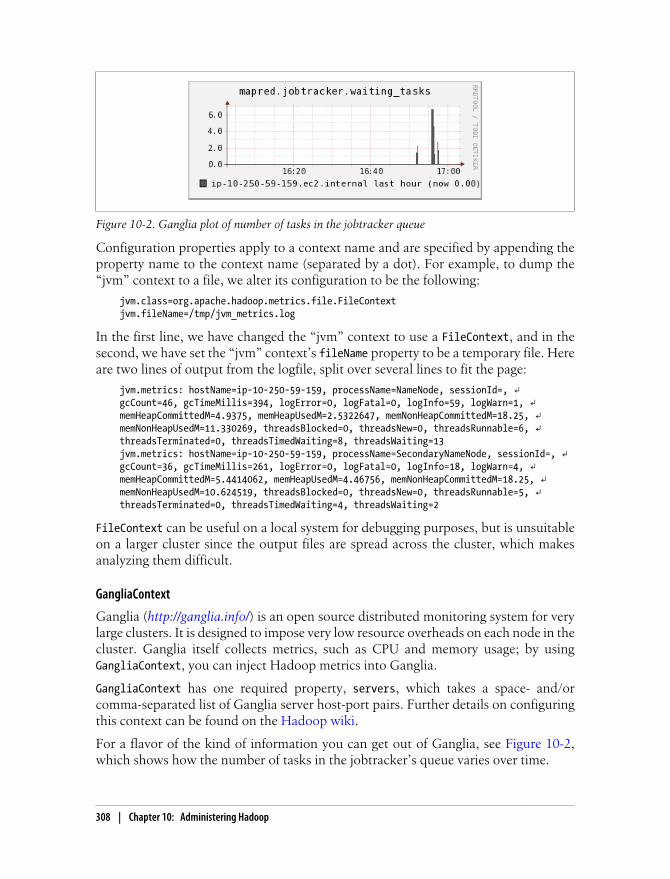
Configuration properties apply to a context name and are specified by appending theproperty name to the context name (separated by a dot). For example, to dump the“jvm” context to a file, we alter its configuration to be the following:

jvm.class=org.apache.hadoop.metrics.file.FileContextjvm.fileName=/tmp/jvm_metrics.log

In the first line, we have changed the “jvm” context to use a FileContext, and in thesecond, we have set the “jvm” context’s fileName property to be a temporary file. Hereare two lines of output from the logfile, split over several lines to fit the page:

jvm.metrics: hostName=ip-10-250-59-159, processName=NameNode, sessionId=, ↵gcCount=46, gcTimeMillis=394, logError=0, logFatal=0, logInfo=59, logWarn=1, ↵memHeapCommittedM=4.9375, memHeapUsedM=2.5322647, memNonHeapCommittedM=18.25, ↵memNonHeapUsedM=11.330269, threadsBlocked=0, threadsNew=0, threadsRunnable=6, ↵threadsTerminated=0, threadsTimedWaiting=8, threadsWaiting=13jvm.metrics: hostName=ip-10-250-59-159, processName=SecondaryNameNode, sessionId=, ↵gcCount=36, gcTimeMillis=261, logError=0, logFatal=0, logInfo=18, logWarn=4, ↵memHeapCommittedM=5.4414062, memHeapUsedM=4.46756, memNonHeapCommittedM=18.25, ↵memNonHeapUsedM=10.624519, threadsBlocked=0, threadsNew=0, threadsRunnable=5, ↵threadsTerminated=0, threadsTimedWaiting=4, threadsWaiting=2

FileContext can be useful on a local system for debugging purposes, but is unsuitableon a larger cluster since the output files are spread across the cluster, which makesanalyzing them difficult.

GangliaContext

Ganglia (http://ganglia.info/) is an open source distributed monitoring system for verylarge clusters. It is designed to impose very low resource overheads on each node in thecluster. Ganglia itself collects metrics, such as CPU and memory usage; by usingGangliaContext, you can inject Hadoop metrics into Ganglia.

GangliaContext has one required property, servers, which takes a space- and/orcomma-separated list of Ganglia server host-port pairs. Further details on configuringthis context can be found on the Hadoop wiki.

For a flavor of the kind of information you can get out of Ganglia, see Figure 10-2,which shows how the number of tasks in the jobtracker’s queue varies over time.

Figure 10-2. Ganglia plot of number of tasks in the jobtracker queue

308 | Chapter 10: Administering Hadoop

NullContextWithUpdateThread

Both FileContext and a GangliaContext push metrics to an external system. However,some monitoring systems—notably JMX—need to pull metrics from Hadoop. NullContextWithUpdateThread is designed for this. Like NullContext, it doesn’t publish anymetrics, but in addition it runs a timer that periodically updates the metrics stored inmemory. This ensures that the metrics are up-to-date when they are fetched by anothersystem.

All implementations of MetricsContext, except NullContext, perform this updatingfunction (and they all expose a period property that defaults to five seconds), so youneed to use NullContextWithUpdateThread only if you are not collecting metrics usinganother output. If you were using GangliaContext, for example, then it would ensurethe metrics are updated, so you would be able to use JMX in addition with no furtherconfiguration of the metrics system. JMX is discussed in more detail shortly.

CompositeContext

CompositeContext allows you to output the same set of metrics to multiple contexts,such as a FileContext and a GangliaContext. The configuration is slightly tricky and isbest shown by an example:

jvm.class=org.apache.hadoop.metrics.spi.CompositeContextjvm.arity=2jvm.sub1.class=org.apache.hadoop.metrics.file.FileContextjvm.fileName=/tmp/jvm_metrics.logjvm.sub2.class=org.apache.hadoop.metrics.ganglia.GangliaContextjvm.servers=ip-10-250-59-159.ec2.internal:8649

The arity property is used to specify the number of subcontexts; in this case, there aretwo. The property names for each subcontext are modified to have a part specifyingthe subcontext number, hence jvm.sub1.class and jvm.sub2.class.

Java Management ExtensionsJava Management Extensions (JMX) is a standard Java API for monitoring and man-aging applications. Hadoop includes several managed beans (MBeans), which exposeHadoop metrics to JMX-aware applications. There are MBeans that expose the metricsin the “dfs” and “rpc” contexts, but none for the “mapred” context (at the time of thiswriting) or the “jvm” context (as the JVM itself exposes a richer set of JVM metrics).These MBeans are listed in Table 10-3.

Monitoring | 309

Table 10-3. Hadoop MBeans

MBean class Daemons Metrics

NameNodeActivityMBean Namenode Namenode activity metrics, such as thenumber of create file operations

FSNamesystemMBean Namenode Namenode status metrics, such as thenumber of connected datanodes

DataNodeActivityMBean Datanode Datanode activity metrics, such as num-ber of bytes read

FSDatasetMBean Datanode Datanode storage metrics, such ascapacity and free storage space

RpcActivityMBean All daemons that use RPC:namenode, datanode,jobtracker, tasktracker

RPC statistics, such as average process-ing time

The JDK comes with a tool called JConsole for viewing MBeans in a running JVM. It’suseful for browsing Hadoop metrics, as demonstrated in Figure 10-3.

Figure 10-3. JConsole view of a locally running namenode, showing metrics for the filesystem state

Although you can see Hadoop metrics via JMX using the default metricsconfiguration, they will not be updated unless you change theMetricsContext implementation to something other than NullContext.For example, NullContextWithUpdateThread is appropriate if JMX is theonly way you will be monitoring metrics.

310 | Chapter 10: Administering Hadoop

Many third-party monitoring and alerting systems (such as Nagios or Hyperic) canquery MBeans, making JMX the natural way to monitor your Hadoop cluster from anexisting monitoring system. You will need to enable remote access to JMX, however,and choose a level of security that is appropriate for your cluster. The options hereinclude password authentication, SSL connections, and SSL client-authentication. Seethe official Java documentation§ for an in-depth guide on configuring these options.

All the options for enabling remote access to JMX involve setting Java system proper-ties, which we do for Hadoop by editing the conf/hadoop-env.sh file. The followingconfiguration settings show how to enable password-authenticated remote access toJMX on the namenode (with SSL disabled). The process is very similar for other Hadoopdaemons:

export HADOOP_NAMENODE_OPTS="-Dcom.sun.management.jmxremote -Dcom.sun.management.jmxremote.ssl=false -Dcom.sun.management.jmxremote.password.file=$HADOOP_CONF_DIR/jmxremote.password -Dcom.sun.management.jmxremote.port=8004 $HADOOP_NAMENODE_OPTS"

The jmxremote.password file lists the usernames and their passwords in plain text; theJMX documentation has further details on the format of this file.

With this configuration, we can use JConsole to browse MBeans on a remote name-node. Alternatively, we can use one of the many JMX tools to retrieve MBean attributevalues. Here is an example of using the “jmxquery” command-line tool (and Nagiosplug-in, available from http://code.google.com/p/jmxquery/) to retrieve the number ofunder-replicated blocks:

% ./check_jmx -U service:jmx:rmi:///jndi/rmi://namenode-host:8004/jmxrmi -O \hadoop:service=NameNode,name=FSNamesystemState -A UnderReplicatedBlocks \-w 100 -c 1000 -username monitorRole -password secretJMX OK - UnderReplicatedBlocks is 0

This command establishes a JMX RMI connection to the host namenode-host on port8004 and authenticates using the given username and password. It reads the attributeUnderReplicatedBlocks of the object named hadoop:service=NameNode,name=FSNamesystemState and prints out its value on the console.‖ The -w and -c options specify warningand critical levels for the value: the appropriate values of these are normally determinedafter operating a cluster for a while.

It’s common to use Ganglia in conjunction with an alerting system like Nagios formonitoring a Hadoop cluster. Ganglia is good for efficiently collecting a large numberof metrics and graphing them, whereas Nagios and similar systems are good at sendingalerts when a critical threshold is reached in any of a smaller set of metrics.

§ http://java.sun.com/javase/6/docs/technotes/guides/management/agent.html

‖ It’s convenient to use JConsole to find the object names of the MBeans that you want to monitor. Note thatMBeans for datanode metrics contain a random identifier in Hadoop 0.20, which makes it difficult to monitorthem in anything but an ad hoc way. This was fixed in Hadoop 0.21.0.

Monitoring | 311

Maintenance

Routine Administration Procedures

Metadata backups

If the namenode’s persistent metadata is lost or damaged, the entire filesystem is ren-dered unusable, so it is critical that backups are made of these files. You should keepmultiple copies of different ages (one hour, one day, one week, and one month, say) toprotect against corruption, either in the copies themselves or in the live files runningon the namenode.

A straightforward way to make backups is to write a script to periodically archive thesecondary namenode’s previous.checkpoint subdirectory (under the directory definedby the fs.checkpoint.dir property) to an offsite location. The script should additionallytest the integrity of the copy. This can be done by starting a local namenode daemonand verifying that it has successfully read the fsimage and edits files into memory (byscanning the namenode log for the appropriate success message, for example).#

Data backups

Although HDFS is designed to store data reliably, data loss can occur, just like in anystorage system, and thus a backup strategy is essential. With the large data volumesthat Hadoop can store, deciding what data to back up and where to store it is a chal-lenge. The key here is to prioritize your data. The highest priority is the data that cannotbe regenerated and that is critical to the business; however, data that is straightforwardto regenerate, or essentially disposable because it is of limited business value, is thelowest priority, and you may choose not to make backups of this category of data.

Do not make the mistake of thinking that HDFS replication is a substi-tute for making backups. Bugs in HDFS can cause replicas to be lost,and so can hardware failures. Although Hadoop is expressly designedso that hardware failure is very unlikely to result in data loss, the pos-sibility can never be completely ruled out, particularly when combinedwith software bugs or human error.

When it comes to backups, think of HDFS in the same way as you wouldRAID. Although the data will survive the loss of an individual RAIDdisk, it may not if the RAID controller fails, or is buggy (perhaps over-writing some data), or the entire array is damaged.

#Hadoop 0.21.0 comes with an Offline Image Viewer, which can be used to check the integrity of the imagefiles.

312 | Chapter 10: Administering Hadoop

It’s common to have a policy for user directories in HDFS. For example, they may havespace quotas and be backed up nightly. Whatever the policy, make sure your usersknow what it is, so they know what to expect.

The distcp tool is ideal for making backups to other HDFS clusters (preferably runningon a different version of the software, to guard against loss due to bugs in HDFS) orother Hadoop filesystems (such as S3 or KFS), since it can copy files in parallel. Alter-natively, you can employ an entirely different storage system for backups, using one ofthe ways to export data from HDFS described in “Hadoop Filesystems” on page 47.

Filesystem check (fsck)

It is advisable to run HDFS’s fsck tool regularly (for example, daily) on the whole file-system to proactively look for missing or corrupt blocks. See “Filesystem check(fsck)” on page 301.

Filesystem balancer

Run the balancer tool (see “balancer” on page 304) regularly to keep the filesystemdatanodes evenly balanced.

Commissioning and Decommissioning NodesAs an administrator of a Hadoop cluster, you will need to add or remove nodes fromtime to time. For example, to grow the storage available to a cluster, you commissionnew nodes. Conversely, sometimes you may wish to shrink a cluster, and to do so, youdecommission nodes. It can sometimes be necessary to decommission a node if it ismisbehaving, perhaps because it is failing more often than it should or its performanceis noticeably slow.

Nodes normally run both a datanode and a tasktracker, and both are typicallycommissioned or decommissioned in tandem.

Commissioning new nodes

Although commissioning a new node can be as simple as configuring the hdfs-site.xml file to point to the namenode and the mapred-site.xml file to point to the job-tracker, and starting the datanode and jobtracker daemons, it is generally best to havea list of authorized nodes.

Maintenance | 313

It is a potential security risk to allow any machine to connect to the namenode and actas a datanode, since the machine may gain access to data that it is not authorized tosee. Furthermore, since such a machine is not a real datanode, it is not under yourcontrol, and may stop at any time, causing potential data loss. (Imagine what wouldhappen if a number of such nodes were connected, and a block of data was presentonly on the “alien” nodes?) This scenario is a risk even inside a firewall, throughmisconfiguration, so datanodes (and tasktrackers) should be explicitly managed on allproduction clusters.

Datanodes that are permitted to connect to the namenode are specified in a file whosename is specified by the dfs.hosts property. The file resides on the namenode’s localfilesystem, and it contains a line for each datanode, specified by network address (asreported by the datanode—you can see what this is by looking at the namenode’s webUI). If you need to specify multiple network addresses for a datanode, put them on oneline, separated by whitespace.

Similarly, tasktrackers that may connect to the jobtracker are specified in a file whosename is specified by the mapred.hosts property. In most cases, there is one shared file,referred to as the include file, that both dfs.hosts and mapred.hosts refer to, since nodesin the cluster run both datanode and tasktracker daemons.

The file (or files) specified by the dfs.hosts and mapred.hosts propertiesis different from the slaves file. The former is used by the namenode andjobtracker to determine which worker nodes may connect. The slavesfile is used by the Hadoop control scripts to perform cluster-wide op-erations, such as cluster restarts. It is never used by the Hadoopdaemons.

To add new nodes to the cluster:

1. Add the network addresses of the new nodes to the include file.

2. Update the namenode with the new set of permitted datanodes using thiscommand:

% hadoop dfsadmin -refreshNodes

3. Update the slaves file with the new nodes, so that they are included in future op-erations performed by the Hadoop control scripts.

4. Start the new datanodes.

5. Restart the MapReduce cluster.*

6. Check that the new datanodes and tasktrackers appear in the web UI.

* At the time of this writing, there is no command to refresh the set of permitted nodes in the jobtracker.Consider setting the mapred.jobtracker.restart.recover property to true to make the jobtracker recoverrunning jobs after a restart.

314 | Chapter 10: Administering Hadoop

HDFS will not move blocks from old datanodes to new datanodes to balance the cluster.To do this, you should run the balancer described in “balancer” on page 304.

Decommissioning old nodes

Although HDFS is designed to tolerate datanode failures, this does not mean you canjust terminate datanodes en masse with no ill effect. With a replication level of three,for example, the chances are very high that you will lose data by simultaneously shuttingdown three datanodes if they are on different racks. The way to decommissiondatanodes is to inform the namenode of the nodes that you wish to take out of circu-lation, so that it can replicate the blocks to other datanodes before the datanodes areshut down.

With tasktrackers, Hadoop is more forgiving. If you shut down a tasktracker that isrunning tasks, the jobtracker will notice the failure and reschedule the tasks on othertasktrackers.

The decommissioning process is controlled by an exclude file, which for HDFS is setby the dfs.hosts.exclude property and for MapReduce by the mapred.hosts.excludeproperty. It is often the case that these properties refer to the same file. The exclude filelists the nodes that are not permitted to connect to the cluster.

The rules for whether a tasktracker may connect to the jobtracker are simple: a task-tracker may connect only if it appears in the include file and does not appear in theexclude file. An unspecified or empty include file is taken to mean that all nodes are inthe include file.

For HDFS, the rules are slightly different. If a datanode appears in both the include andthe exclude file, then it may connect, but only to be decommissioned. Table 10-4 sum-marizes the different combinations for datanodes. As for tasktrackers, an unspecifiedor empty include file means all nodes are included.

Table 10-4. HDFS include and exclude file precedence

Node appears in include file Node appears in exclude file Interpretation

No No Node may not connect.

No Yes Node may not connect.

Yes No Node may connect.

Yes Yes Node may connect and will be decommissioned.

To remove nodes from the cluster:

1. Add the network addresses of the nodes to be decommissioned to the exclude file.Do not update the include file at this point.

2. Restart the MapReduce cluster to stop the tasktrackers on the nodes beingdecommissioned.

Maintenance | 315

3. Update the namenode with the new set of permitted datanodes, with thiscommand:

% hadoop dfsadmin -refreshNodes

4. Go to the web UI and check whether the admin state has changed to “Decommis-sion In Progress” for the datanodes being decommissioned. They will start copyingtheir blocks to other datanodes in the cluster.

5. When all the datanodes report their state as “Decommissioned,” then all the blockshave been replicated. Shut down the decommissioned nodes.

6. Remove the nodes from the include file, and run:

% hadoop dfsadmin -refreshNodes

7. Remove the nodes from the slaves file.

UpgradesUpgrading an HDFS and MapReduce cluster requires careful planning. The most im-portant consideration is the HDFS upgrade. If the layout version of the filesystem haschanged, then the upgrade will automatically migrate the filesystem data and metadatato a format that is compatible with the new version. As with any procedure that involvesdata migration, there is a risk of data loss, so you should be sure that both your dataand metadata is backed up (see “Routine Administration Procedures” on page 312).

Part of the planning process should include a trial run on a small test cluster with acopy of data that you can afford to lose. A trial run will allow you to familiarize yourselfwith the process, customize it to your particular cluster configuration and toolset, andiron out any snags before running the upgrade procedure on a production cluster. Atest cluster also has the benefit of being available to test client upgrades on.

Version CompatibilityAll pre-1.0 Hadoop components have very rigid version compatibility requirements.Only components from the same release are guaranteed to be compatible with eachother, which means the whole system—from daemons to clients—has to be upgradedsimultaneously, in lockstep. This necessitates a period of cluster downtime.

Version 1.0 of Hadoop promises to loosen these requirements so that, for example,older clients can talk to newer servers (within the same major release number). In laterreleases, rolling upgrades may be supported, which would allow cluster daemons to beupgraded in phases, so that the cluster would still be available to clients during theupgrade.

Upgrading a cluster when the filesystem layout has not changed is fairlystraightforward: install the new versions of HDFS and MapReduce on the cluster (andon clients at the same time), shut down the old daemons, update configuration files,

316 | Chapter 10: Administering Hadoop

then start up the new daemons and switch clients to use the new libraries. This processis reversible, so rolling back an upgrade is also straightforward.

After every successful upgrade, you should perform a couple of final cleanup steps:

• Remove the old installation and configuration files from the cluster.

• Fix any deprecation warnings in your code and configuration.

HDFS data and metadata upgrades

If you use the procedure just described to upgrade to a new version of HDFS and itexpects a different layout version, then the namenode will refuse to run. A message likethe following will appear in its log:

File system image contains an old layout version -16.An upgrade to version -18 is required.Please restart NameNode with -upgrade option.

The most reliable way of finding out whether you need to upgrade the filesystem is byperforming a trial on a test cluster.

An upgrade of HDFS makes a copy of the previous version’s metadata and data. Doingan upgrade does not double the storage requirements of the cluster, as the datanodesuse hard links to keep two references (for the current and previous version) to the sameblock of data. This design makes it straightforward to roll back to the previous versionof the filesystem, should you need to. You should understand that any changes madeto the data on the upgraded system will be lost after the rollback completes.

You can keep only the previous version of the filesystem: you can’t roll back severalversions. Therefore, to carry out another upgrade to HDFS data and metadata, you willneed to delete the previous version, a process called finalizing the upgrade. Once anupgrade is finalized, there is no procedure for rolling back to a previous version.

In general, you can skip releases when upgrading (for example, you can upgrade fromrelease 0.18.3 to 0.20.0 without having to upgrade to a 0.19.x release first), but in somecases, you may have to go through intermediate releases. The release notes make it clearwhen this is required.

You should only attempt to upgrade a healthy filesystem. Before running the upgrade,do a full fsck (see “Filesystem check (fsck)” on page 301). As an extra precaution, youcan keep a copy of the fsck output that lists all the files and blocks in the system, soyou can compare it with the output of running fsck after the upgrade.

It’s also worth clearing out temporary files before doing the upgrade, both from theMapReduce system directory on HDFS and local temporary files.

With these preliminaries out of the way, here is the high-level procedure for upgradinga cluster when the filesystem layout needs to be migrated:

1. Make sure that any previous upgrade is finalized before proceeding with anotherupgrade.

Maintenance | 317

2. Shut down MapReduce and kill any orphaned task processes on the tasktrackers.

3. Shut down HDFS and backup the namenode directories.

4. Install new versions of Hadoop HDFS and MapReduce on the cluster and onclients.

5. Start HDFS with the -upgrade option.

6. Wait until the upgrade is complete.

7. Perform some sanity checks on HDFS.

8. Start MapReduce.

9. Roll back or finalize the upgrade (optional).

While running the upgrade procedure, it is a good idea to remove the Hadoop scriptsfrom your PATH environment variable. This forces you to be explicit about which versionof the scripts you are running. It can be convenient to define two environment variablesfor the new installation directories; in the following instructions, we have definedOLD_HADOOP_INSTALL and NEW_HADOOP_INSTALL.

To perform the upgrade, run the following command (this is step 5 inthe high-level upgrade procedure):

% $NEW_HADOOP_INSTALL/bin/start-dfs.sh -upgrade

This causes the namenode to upgrade its metadata, placing the previous version in anew directory called previous:

${dfs.name.dir}/current/VERSION /edits /fsimage /fstime /previous/VERSION /edits /fsimage /fstime

Similarly, datanodes upgrade their storage directories, preserving the old copy in adirectory called previous.

The upgrade process is not instantaneous, but you cancheck the progress of an upgrade using dfsadmin (upgrade events also appear in thedaemons’ logfiles, step 6):

% $NEW_HADOOP_INSTALL/bin/hadoop dfsadmin -upgradeProgress statusUpgrade for version -18 has been completed.Upgrade is not finalized.

This shows that the upgrade is complete. At this stage, you should runsome sanity checks (step 7) on the filesystem (check files and blocks using fsck, basicfile operations). You might choose to put HDFS into safe mode while you are runningsome of these checks (the ones that are read-only) to prevent others from makingchanges.

Start the upgrade.

Wait until the upgrade is complete.

Check the upgrade.

318 | Chapter 10: Administering Hadoop

If you find that the new version is not working correctly,you may choose to roll back to the previous version (step 9). This is only possible ifyou have not finalized the upgrade.

A rollback reverts the filesystem state to before the upgrade was per-formed, so any changes made in the meantime will be lost. In otherwords, it rolls back to the previous state of the filesystem, rather thandowngrading the current state of the filesystem to a former version.

First, shut down the new daemons:

% $NEW_HADOOP_INSTALL/bin/stop-dfs.sh

Then start up the old version of HDFS with the -rollback option:

% $OLD_HADOOP_INSTALL/bin/start-dfs.sh -rollback

This command gets the namenode and datanodes to replace their current storagedirectories with their previous copies. The filesystem will be returned to its previousstate.

When you are happy with the new version of HDFS, youcan finalize the upgrade (step 9) to remove the previous storage directories.

After an upgrade has been finalized, there is no way to roll back to theprevious version.

This step is required before performing another upgrade:

% $NEW_HADOOP_INSTALL/bin/hadoop dfsadmin -finalizeUpgrade% $NEW_HADOOP_INSTALL/bin/hadoop dfsadmin -upgradeProgress statusThere are no upgrades in progress.

HDFS is now fully upgraded to the new version.

Roll back the upgrade (optional).

Finalize the upgrade (optional).

Maintenance | 319

CHAPTER 11

Pig

Pig raises the level of abstraction for processing large datasets. MapReduce allows youthe programmer to specify a map function followed by a reduce function, but workingout how to fit your data processing into this pattern, which often requires multipleMapReduce stages, can be a challenge. With Pig, the data structures are much richer,typically being multivalued and nested; and the set of transformations you can applyto the data are much more powerful—they include joins, for example, which are notfor the faint of heart in MapReduce.

Pig is made up of two pieces:

• The language used to express data flows, called Pig Latin.

• The execution environment to run Pig Latin programs. There are currently twoenvironments: local execution in a single JVM and distributed execution on a Ha-doop cluster.

A Pig Latin program is made up of a series of operations, or transformations, that areapplied to the input data to produce output. Taken as a whole, the operations describea data flow, which the Pig execution environment translates into an executable repre-sentation and then runs. Under the covers, Pig turns the transformations into a seriesof MapReduce jobs, but as a programmer you are mostly unaware of this, which allowsyou to focus on the data rather than the nature of the execution.

Pig is a scripting language for exploring large datasets. One criticism of MapReduce isthat the development cycle is very long. Writing the mappers and reducers, compilingand packaging the code, submitting the job(s), and retrieving the results is a time-consuming business, and even with Streaming, which removes the compile and packagestep, the experience is still involved. Pig’s sweet spot is its ability to process terabytesof data simply by issuing a half-dozen lines of Pig Latin from the console. Indeed, itwas created at Yahoo! to make it easier for researchers and engineers to mine the hugedatasets there. Pig is very supportive of a programmer writing a query, since it providesseveral commands for introspecting the data structures in your program, as it is written.Even more useful, it can perform a sample run on a representative subset of your input

321

data, so you can see whether there are errors in the processing before unleashing it onthe full dataset.

Pig was designed to be extensible. Virtually all parts of the processing path are cus-tomizable: loading, storing, filtering, grouping, and joining can all be altered by user-defined functions (UDFs). These functions operate on Pig’s nested data model, so theycan integrate very deeply with Pig’s operators. As another benefit, UDFs tend to bemore reusable than the libraries developed for writing MapReduce programs.

Pig isn’t suitable for all data processing tasks, however. Like MapReduce, it is designedfor batch processing of data. If you want to perform a query that touches only a smallamount of data in a large dataset, then Pig will not perform well, since it is set up toscan the whole dataset, or at least large portions of it.

In some cases, Pig doesn’t perform as well as programs written in MapReduce. How-ever, the gap is narrowing with each release, as the Pig team implements sophisticatedalgorithms for implementing Pig’s relational operators. It’s fair to say that unless youare willing to invest a lot of effort optimizing Java MapReduce code, writing queries inPig Latin will save you time.

Installing and Running PigPig runs as a client-side application. Even if you want to run Pig on a Hadoop cluster,there is nothing extra to install on the cluster: Pig launches jobs and interacts withHDFS (or other Hadoop filesystems) from your workstation.

Installation is straightforward. Java 6 is a prerequisite (and on Windows, you will needCygwin). Download a stable release from http://hadoop.apache.org/pig/releases.html,and unpack the tarball in a suitable place on your workstation:

% tar xzf pig-x.y.z.tar.gz

It’s convenient to add Pig’s binary directory to your command-line path. For example:

% export PIG_INSTALL=/home/tom/pig-x.y.z% export PATH=$PATH:$PIG_INSTALL/bin

You also need to set the JAVA_HOME environment variable to point to a suitable Javainstallation.

Try typing pig -help to get usage instructions.

Execution TypesPig has two execution types or modes: local mode and MapReduce mode.

322 | Chapter 11: Pig

Local mode

In local mode, Pig runs in a single JVM and accesses the local filesystem. This mode issuitable only for small datasets and when trying out Pig.

The execution type is set using the -x or -exectype option. To run in local mode, setthe option to local:

% pig -x localgrunt>

This starts Grunt, the Pig interactive shell, which is discussed in more detail shortly.

MapReduce mode

In MapReduce mode, Pig translates queries into MapReduce jobs and runs them on aHadoop cluster. The cluster may be a pseudo- or fully distributed cluster. MapReducemode (with a fully distributed cluster) is what you use when you want to run Pig onlarge datasets.

To use MapReduce mode, you first need to check that the version of Pig you down-loaded is compatible with the version of Hadoop you are using. Pig releases will onlywork against particular versions of Hadoop; this is documented on the releases page.For example, Pig 0.3 and 0.4 run against a Hadoop 0.18.x release, while Pig 0.5 to 0.7work with Hadoop 0.20.x.

If a Pig release supports multiple versions of Hadoop, you can use the environmentvariable PIG_HADOOP_VERSION to tell Pig the version of Hadoop it is connecting to. Forexample, the following makes Pig use any 0.18.x version of Hadoop:

% export PIG_HADOOP_VERSION=18

Next, you need to point Pig at the cluster’s namenode and jobtracker. If you alreadyhave a Hadoop site file (or files) that define fs.default.name and mapred.job.tracker,you can simply add Hadoop’s configuration directory to Pig’s classpath:

% export PIG_CLASSPATH=$HADOOP_INSTALL/conf/

Alternatively, you can set these two properties in the pig.properties file in Pig’s confdirectory. Here’s an example for a pseudo-distributed setup:

fs.default.name=hdfs://localhost/mapred.job.tracker=localhost:8021

Once you have configured Pig to connect to a Hadoop cluster, you can launch Pig,setting the -x option to mapreduce, or omitting it entirely, as MapReduce mode is thedefault:

% pig10/07/16 16:27:37 INFO pig.Main: Logging error messages to: /Users/tom/dev/pig-0.7.0/pig_1279294057867.log2010-07-16 16:27:38,243 [main] INFO org.apache.pig.backend.hadoop.executionengine.HExecutionEngine - Connecting to hadoop file system at: hdfs://localhost/2010-07-16 16:27:38,741 [main] INFO org.apache.pig.backend.hadoop.executionengi

Installing and Running Pig | 323

ne.HExecutionEngine - Connecting to map-reduce job tracker at: localhost:8021grunt>

As you can see from the output, Pig reports the filesystem and jobtracker that it hasconnected to.

Running Pig ProgramsThere are three ways of executing Pig programs, all of which work in both local andMapReduce mode:

ScriptPig can run a script file that contains Pig commands. For example, pigscript.pig runs the commands in the local file script.pig. Alternatively, for veryshort scripts, you can use the -e option to run a script specified as a string on thecommand line.

GruntGrunt is an interactive shell for running Pig commands. Grunt is started when nofile is specified for Pig to run, and the -e option is not used. It is also possible torun Pig scripts from within Grunt using run and exec.

EmbeddedYou can run Pig programs from Java, much like you can use JDBC to run SQLprograms from Java. There are more details on the Pig wiki at http://wiki.apache.org/pig/EmbeddedPig.

GruntGrunt has line-editing facilities like those found in GNU Readline (used in the bashshell and many other command-line applications). For instance, the Ctrl-E key com-bination will move the cursor to the end of the line. Grunt remembers command his-tory, too,* and you can recall lines in the history buffer using Ctrl-P or Ctrl-N (forprevious and next) or, equivalently, the up or down cursor keys.

Another handy feature is Grunt’s completion mechanism, which will try to completePig Latin keywords and functions when you press the Tab key. For example, considerthe following incomplete line:

grunt> a = foreach b ge

If you press the Tab key at this point, ge will expand to generate, a Pig Latin keyword:

grunt> a = foreach b generate

You can customize the completion tokens by creating a file named autocomplete andplacing it on Pig’s classpath (such as in the conf directory in Pig’s install directory), or

* History is stored in a file called .pig_history in your home directory.

324 | Chapter 11: Pig

in the directory you invoked Grunt from. The file should have one token per line, andtokens must not contain any whitespace. Matching is case-sensitive. It can be veryhandy to add commonly used file paths (especially because Pig does not perform file-name completion) or the names of any user-defined functions you have created.

You can get a list of commands using the help command. When you’ve finished yourGrunt session, you can exit with the quit command.

Pig Latin EditorsPigPen is an Eclipse plug-in that provides an environment for developing Pig programs.It includes a Pig script text editor, an example generator (equivalent to the ILLUS-TRATE command), and a button for running the script on a Hadoop cluster. There isalso an operator graph window, which shows a script in graph form, for visualizing thedata flow. For full installation and usage instructions, please refer to the Pig wiki athttp://wiki.apache.org/pig/PigPen.

There are also Pig Latin syntax highlighters for other editors, including Vim and Text-Mate. Details are available on the Pig wiki.

An ExampleLet’s look at a simple example by writing the program to calculate the maximumrecorded temperature by year for the weather dataset in Pig Latin (just like we did usingMapReduce in Chapter 2). The complete program is only a few lines long:

-- max_temp.pig: Finds the maximum temperature by yearrecords = LOAD 'input/ncdc/micro-tab/sample.txt' AS (year:chararray, temperature:int, quality:int);filtered_records = FILTER records BY temperature != 9999 AND (quality == 0 OR quality == 1 OR quality == 4 OR quality == 5 OR quality == 9);grouped_records = GROUP filtered_records BY year;max_temp = FOREACH grouped_records GENERATE group, MAX(filtered_records.temperature);DUMP max_temp;

To explore what’s going on, we’ll use Pig’s Grunt interpreter, which allows us to enterlines and interact with the program to understand what it’s doing. Start up Grunt inlocal mode, then enter the first line of the Pig script:

grunt> records = LOAD 'input/ncdc/micro-tab/sample.txt'>> AS (year:chararray, temperature:int, quality:int);

For simplicity, the program assumes that the input is tab-delimited text, with each linehaving just year, temperature, and quality fields. (Pig actually has more flexibility thanthis with regard to the input formats it accepts, as you’ll see later.) This line describesthe input data we want to process. The year:chararray notation describes the field’sname and type; a chararray is like a Java string, and an int is like a Java int. The LOADoperator takes a URI argument; here we are just using a local file, but we could refer

An Example | 325

to an HDFS URI. The AS clause (which is optional) gives the fields names to make itconvenient to refer to them in subsequent statements.

The result of the LOAD operator, indeed any operator in Pig Latin, is a relation, whichis just a set of tuples. A tuple is just like a row of data in a database table, with multiplefields in a particular order. In this example, the LOAD function produces a set of (year,temperature, quality) tuples that are present in the input file. We write a relation withone tuple per line, where tuples are represented as comma-separated items inparentheses:

(1950,0,1)(1950,22,1)(1950,-11,1)(1949,111,1)

Relations are given names, or aliases, so they can be referred to. This relation is giventhe records alias. We can examine the contents of an alias using the DUMP operator:

grunt> DUMP records;(1950,0,1)(1950,22,1)(1950,-11,1)(1949,111,1)(1949,78,1)

We can also see the structure of a relation—the relation’s schema—using the DESCRIBE operator on the relation’s alias:

grunt> DESCRIBE records;records: {year: chararray,temperature: int,quality: int}

This tells us that records has three fields, with aliases year, temperature, and quality,which are the names we gave them in the AS clause. The fields have the types given tothem in the AS clause, too. We shall examine types in Pig in more detail later.

The second statement removes records that have a missing temperature (indicated bya value of 9999) or an unsatisfactory quality reading. For this small dataset, no recordsare filtered out:

grunt> filtered_records = FILTER records BY temperature != 9999 AND>> (quality == 0 OR quality == 1 OR quality == 4 OR quality == 5 OR quality == 9);grunt> DUMP filtered_records;(1950,0,1)(1950,22,1)(1950,-11,1)(1949,111,1)(1949,78,1)

The third statement uses the GROUP function to group the records relation by theyear field. Let’s use DUMP to see what it produces:

grunt> grouped_records = GROUP filtered_records BY year;grunt> DUMP grouped_records;(1949,{(1949,111,1),(1949,78,1)})(1950,{(1950,0,1),(1950,22,1),(1950,-11,1)})

326 | Chapter 11: Pig

We now have two rows, or tuples, one for each year in the input data. The first field ineach tuple is the field being grouped by (the year), and the second field is a bag of tuplesfor that year. A bag is just an unordered collection of tuples, which in Pig Latin isrepresented using curly braces.

By grouping the data in this way, we have created a row per year, so now all that remainsis to find the maximum temperature for the tuples in each bag. Before we do this, let’sunderstand the structure of the grouped_records relation:

grunt> DESCRIBE grouped_records;grouped_records: {group: chararray,filtered_records: {year: chararray,temperature: int,quality: int}}

This tells us that the grouping field is given the alias group by Pig, and the second fieldis the same structure as the filtered_records relation that was being grouped. Withthis information, we can try the fourth transformation:

grunt> max_temp = FOREACH grouped_records GENERATE group,>> MAX(filtered_records.temperature);

FOREACH processes every row to generate a derived set of rows, using a GENERATEclause to define the fields in each derived row. In this example, the first field isgroup, which is just the year. The second field is a little more complex.The filtered_records.temperature reference is to the temperature field of thefiltered_records bag in the grouped_records relation. MAX is a built-in function forcalculating the maximum value of fields in a bag. In this case, it calculates the maximumtemperature for the fields in each filtered_records bag. Let’s check the result:

grunt> DUMP max_temp;(1949,111)(1950,22)

So we’ve successfully calculated the maximum temperature for each year.

Generating ExamplesIn this example, we’ve used a small sample dataset with just a handful of rows to makeit easier to follow the data flow and aid debugging. Creating a cut-down dataset is anart, as ideally it should be rich enough to cover all the cases to exercise your queries(the completeness property), yet be small enough to reason about by the programmer(the conciseness property). Using a random sample doesn’t work well in general, sincejoin and filter operations tend to remove all random data, leaving an empty result,which is not illustrative of the general flow.

With the ILLUSTRATE operator, Pig provides a tool for generating a reasonably com-plete and concise dataset. Although it can’t generate examples for all queries (it doesn’tsupport LIMIT, SPLIT, or nested FOREACH statements, for example), it can generateuseful examples for many queries. ILLUSTRATE works only if the relation has aschema.

An Example | 327

Here is the output from running ILLUSTRATE (slightly reformatted to fit the page):

grunt> ILLUSTRATE max_temp;-------------------------------------------------------------------------------| records | year: bytearray | temperature: bytearray | quality: bytearray | -------------------------------------------------------------------------------| | 1949 | 9999 | 1 | | | 1949 | 111 | 1 | | | 1949 | 78 | 1 | --------------------------------------------------------------------------------------------------------------------------------------------------| records | year: chararray | temperature: int | quality: int | -------------------------------------------------------------------| | 1949 | 9999 | 1 | | | 1949 | 111 | 1 | | | 1949 | 78 | 1 | -----------------------------------------------------------------------------------------------------------------------------------------------| filtered_records | year: chararray | temperature: int | quality: int | ----------------------------------------------------------------------------| | 1949 | 111 | 1 | | | 1949 | 78 | 1 | ----------------------------------------------------------------------------------------------------------------------------------------------------------------| grouped_records | group: chararray | filtered_records: bag({year: chararray, | temperature: int,quality: int}) | ------------------------------------------------------------------------------------| | 1949 | {(1949, 111, 1), (1949, 78, 1)} |-------------------------------------------------------------------------------------------------------------------------------| max_temp | group: chararray | int | -------------------------------------------| | 1949 | 111 | -------------------------------------------

Notice that Pig used some of the original data (this is important to keep the generateddataset realistic), as well as creating some new data. It noticed the special value 9999in the query and created a tuple containing this value to exercise the FILTER statement.

In summary, the output of the ILLUSTRATE is easy to follow and can help you un-derstand what your query is doing.

Comparison with DatabasesHaving seen Pig in action, it might seem that Pig Latin is similar to SQL. The presenceof such operators as GROUP BY and DESCRIBE reinforces this impression. However,there are several differences between the two languages, and between Pig and RDBMSsin general.

328 | Chapter 11: Pig

The most significant difference is that Pig Latin is a data flow programming language,whereas SQL is a declarative programming language. In other words, a Pig Latin pro-gram is a step-by-step set of operations on an input relation, in which each step is asingle transformation. By contrast, SQL statements are a set of constraints that, takentogether, define the output. In many ways, programming in Pig Latin is like workingat the level of an RDBMS query planner, which figures out how to turn a declarativestatement into a system of steps.

RDBMSs store data in tables, with tightly predefined schemas. Pig is more relaxed aboutthe data that it processes: you can define a schema at runtime, but it’s optional. Es-sentially, it will operate on any source of tuples (although the source should supportbeing read in parallel, by being in multiple files, for example), where a UDF is used toread the tuples from their raw representation.† The most common representation is atext file with tab-separated fields, and Pig provides a built-in load function for thisformat. Unlike with a traditional database, there is no data import process to load thedata into the RDBMS. The data is loaded from the filesystem (usually HDFS) as thefirst step in the processing.

Pig’s support for complex, nested data structures differentiates it from SQL, whichoperates on flatter data structures. Also, Pig’s ability to use UDFs and streaming op-erators that are tightly integrated with the language and Pig’s nested data structuresmakes Pig Latin more customizable than most SQL dialects.

There are several features to support online, low-latency queries that RDBMSs havethat are absent in Pig, such as transactions and indexes. As mentioned earlier, Pig doesnot support random reads or queries in the order of tens of milliseconds. Nor does itsupport random writes to update small portions of data; all writes are bulk, streamingwrites, just like MapReduce.

Hive (covered in Chapter 12) sits between Pig and conventional RDBMSs. Like Pig,Hive is designed to use HDFS for storage, but otherwise there are some significantdifferences. Its query language, HiveQL, is based on SQL, and anyone who is familiarwith SQL would have little trouble writing queries in HiveQL. Like RDBMSs, Hivemandates that all data be stored in tables, with a schema under its management; how-ever, it can associate a schema with preexisting data in HDFS, so the load step isoptional. Hive does not support low-latency queries, a characteristic it shares with Pig.

† Or as the Pig Philosophy has it, “Pigs eat anything.”

Comparison with Databases | 329

Pig LatinThis section gives an informal description of the syntax and semantics of the Pig Latinprogramming language.‡ It is not meant to offer a complete reference to thelanguage,§ but there should be enough here for you to get a good understanding of PigLatin’s constructs.

StructureA Pig Latin program consists of a collection of statements. A statement can be thoughtof as an operation, or a command.‖ For example, a GROUP operation is a type ofstatement:

grouped_records = GROUP records BY year;

The command to list the files in a Hadoop filesystem is another example of a statement:

ls /

Statements are usually terminated with a semicolon, as in the example of the GROUPstatement. In fact, this is an example of a statement that must be terminated with asemicolon: it is a syntax error to omit it. The ls command, on the other hand, does nothave to be terminated with a semicolon. As a general guideline, statements or com-mands for interactive use in Grunt do not need the terminating semicolon. This groupincludes the interactive Hadoop commands, as well as the diagnostic operators likeDESCRIBE. It’s never an error to add a terminating semicolon, so if in doubt, it’s sim-plest to add one.

Statements that have to be terminated with a semicolon can be split across multiplelines for readability:

records = LOAD 'input/ncdc/micro-tab/sample.txt' AS (year:chararray, temperature:int, quality:int);

Pig Latin has two forms of comments. Double hyphens are single-line comments.Everything from the first hyphen to the end of the line is ignored by the Pig Latininterpreter:

-- My programDUMP A; -- What's in A?

‡ Not to be confused with Pig Latin, the language game. English words are translated into Pig Latin by movingthe initial consonant sound to the end of the word and adding an “ay” sound. For example, “pig” becomes“ig-pay,” and “Hadoop” becomes “Adoop-hay.”

§ Pig Latin does not have a formal language definition as such, but there is a comprehensive guide to thelanguage that can be found linked to from the Pig wiki at http://wiki.apache.org/pig/.

‖ You sometimes see these terms being used interchangeably in documentation on Pig Latin. For example,“GROUP command, ” “GROUP operation,” “GROUP statement.”

330 | Chapter 11: Pig

C-style comments are more flexible since they delimit the beginning and end of thecomment block with /* and */ markers. They can span lines or be embedded in a singleline:

/* * Description of my program spanning * multiple lines. */A = LOAD 'input/pig/join/A';B = LOAD 'input/pig/join/B';C = JOIN A BY $0, /* ignored */ B BY $1;DUMP C;

Pig Latin has a list of keywords that have a special meaning in the language and cannotbe used as identifiers. These include the operators (LOAD, ILLUSTRATE), commands(cat, ls), expressions (matches, FLATTEN), and functions (DIFF, MAX)—all of whichare covered in the following sections.

Pig Latin has mixed rules on case sensitivity. Operators and commands are not case-sensitive (to make interactive use more forgiving); however, aliases and function namesare case-sensitive.

StatementsAs a Pig Latin program is executed, each statement is parsed in turn. If there are syntaxerrors, or other (semantic) problems such as undefined aliases, the interpreter will haltand display an error message. The interpreter builds a logical plan for every relationaloperation, which forms the core of a Pig Latin program. The logical plan for the state-ment is added to the logical plan for the program so far, then the interpreter moves onto the next statement.

It’s important to note that no data processing takes place while the logical plan of theprogram is being constructed. For example, consider again the Pig Latin program fromthe first example:

-- max_temp.pig: Finds the maximum temperature by yearrecords = LOAD 'input/ncdc/micro-tab/sample.txt' AS (year:chararray, temperature:int, quality:int);filtered_records = FILTER records BY temperature != 9999 AND (quality == 0 OR quality == 1 OR quality == 4 OR quality == 5 OR quality == 9);grouped_records = GROUP filtered_records BY year;max_temp = FOREACH grouped_records GENERATE group, MAX(filtered_records.temperature);DUMP max_temp;

When the Pig Latin interpreter sees the first line containing the LOAD statement, itconfirms that it is syntactically and semantically correct, and adds it to the logical plan,but it does not load the data from the file (or even check whether the file exists). Indeed,where would it load it? Into memory? Even if it did fit into memory, what would it dowith the data? Perhaps not all the input data is needed (since later statements filter it,

Pig Latin | 331

for example), so it would be pointless to load it. The point is that it makes no sense tostart any processing until the whole flow is defined. Similarly, Pig validates the GROUPand FOREACH...GENERATE statements, and adds them to the logical plan withoutexecuting them. The trigger for Pig to start execution is the DUMP statement. At thatpoint, the logical plan is compiled into a physical plan and executed.

Multiquery executionSince DUMP is a diagnostic tool, it will always trigger execution. However, the STOREcommand is different. In interactive mode, STORE acts like DUMP and will alwaystrigger execution (this includes the run command), but in batch mode it will not (thisincludes the exec command). The reason for this is efficiency. In batch mode, Pig willparse the whole script to see if there are any optimizations that could be made to limitthe amount of data to be written to or read from disk. Consider the following simpleexample:

A = LOAD 'input/pig/multiquery/A';B = FILTER A BY $1 == 'banana';C = FILTER A BY $1 != 'banana';STORE B INTO 'output/b';STORE C INTO 'output/c';

Relations B and C are both derived from A, so to save reading A twice, Pig can run thisscript as a single MapReduce job by reading A once and writing two output files fromthe job, one for each of B and C. This feature is called multiquery execution.

In previous versions of Pig that did not have multiquery execution, each STORE state-ment in a script run in batch mode triggered execution, resulting in a job for eachSTORE statement. It is possible to restore the old behavior by disabling multiqueryexecution with the -M or -no_multiquery option to pig.

The physical plan that Pig prepares is a series of MapReduce jobs, which in local modePig runs in the local JVM, and in MapReduce mode Pig runs on a Hadoop cluster.

You can see the logical and physical plans created by Pig using theEXPLAIN command on a relation (EXPLAIN max_temp; for example).

EXPLAIN will also show the MapReduce plan, which shows how thephysical operators are grouped into MapReduce jobs. This is a goodway to find out how many MapReduce jobs Pig will run for your query.

The relational operators that can be a part of a logical plan in Pig are summarized inTable 11-1. We shall go through the operators in more detail in “Data Processing Op-erators” on page 351.

332 | Chapter 11: Pig

Table 11-1. Pig Latin relational operators

Category Operator Description

Loading and storing LOAD Loads data from the filesystem or other storage into a relation

STORE Saves a relation to the filesystem or other storage

DUMP Prints a relation to the console

Filtering FILTER Removes unwanted rows from a relation

DISTINCT Removes duplicate rows from a relation

FOREACH...GENERATE Adds or removes fields from a relation

STREAM Transforms a relation using an external program

SAMPLE Selects a random sample of a relation

Grouping and joining JOIN Joins two or more relations

COGROUP Groups the data in two or more relations

GROUP Groups the data in a single relation

CROSS Creates the cross-product of two or more relations

Sorting ORDER Sorts a relation by one or more fields

LIMIT Limits the size of a relation to a maximum number of tuples

Combining and splitting UNION Combines two or more relations into one

SPLIT Splits a relation into two or more relations

There are other types of statements that are not added to the logical plan. For example,the diagnostic operators, DESCRIBE, EXPLAIN, and ILLUSTRATE are provided toallow the user to interact with the logical plan, for debugging purposes (see Ta-ble 11-2). DUMP is a sort of diagnostic operator, too, since it is used only to allowinteractive debugging of small result sets or in combination with LIMIT to retrieve afew rows from a larger relation. The STORE statement should be used when the sizeof the output is more than a few lines, as it writes to a file, rather than to the console.

Table 11-2. Pig Latin diagnostic operators

Operator Description

DESCRIBE Prints a relation’s schema

EXPLAIN Prints the logical and physical plans

ILLUSTRATE Shows a sample execution of the logical plan, using a generated subset of the input

Pig Latin provides two statements, REGISTER and DEFINE, to make it possible toincorporate user-defined functions into Pig scripts (see Table 11-3).

Pig Latin | 333

Table 11-3. Pig Latin UDF statements

Statement Description

REGISTER Registers a JAR file with the Pig runtime

DEFINE Creates an alias for a UDF, streaming script, or a command specification

Since they do not process relations, commands are not added to the logical plan; in-stead, they are executed immediately. Pig provides commands to interact with Hadoopfilesystems (which are very handy for moving data around before or after processingwith Pig) and MapReduce, as well as a few utility commands (described in Table 11-4).

Table 11-4. Pig Latin commands

Category Command Description

Hadoop Filesystem cat Prints the contents of one or more files

cd Changes the current directory

copyFromLocal Copies a local file or directory to a Hadoop filesystem

copyToLocal Copies a file or directory on a Hadoop filesystem to the local filesystem

cp Copies a file or directory to another directory

fs Accesses Hadoop’s filesystem shell

ls Lists files

mkdir Creates a new directory

mv Moves a file or directory to another directory

pwd Prints the path of the current working directory

rm Deletes a file or directory

rmf Forcibly deletes a file or directory (does not fail if the file or directory does not exist)

Hadoop MapReduce kill Kills a MapReduce job

Utility exec Runs a script in a new Grunt shell in batch mode

help Shows the available commands and options

quit Exits the interpreter

run Runs a script within the existing Grunt shell

set Sets Pig options

The filesystem commands can operate on files or directories in any Hadoop filesystem,and they are very similar to the hadoop fs commands (which is not surprising, as bothare simple wrappers around the Hadoop FileSystem interface). You can access all ofthe Hadoop filesystem shell commands using Pig’s fs command. For example,fs -ls will show a file listing, and fs -help will show help on all the availablecommands.

334 | Chapter 11: Pig

Precisely which Hadoop filesystem is used is determined by the fs.default.name prop-erty in the site file for Hadoop Core. See “The Command-Line Interface” on page 45for more details on how to configure this property.

These commands are mostly self-explanatory, except set, which is used to set optionsthat control Pig’s behavior. The debug option is used to turn debug logging on or offfrom within a script (you can also control the log level when launching Pig, using the-d or -debug option):

grunt> set debug on

Another useful option is the job.name option, which gives a Pig job a meaningful name,making it easier to pick out your Pig MapReduce jobs when running on a shared Ha-doop cluster. If Pig is running a script (rather than being an interactive query fromGrunt), its job name defaults to a value based on the script name.

There are two commands in Table 11-4 for running a Pig script, exec and run. Thedifference is that exec runs the script in batch mode in a new Grunt shell, so any aliasesdefined in the script are not accessible to the shell after the script has completed. Onthe other hand, when running a script with run, it is as if the contents of the script hadbeen entered manually, so the command history of the invoking shell contains all thestatements from the script. Multiquery execution, where Pig executes a batch of state-ments in one go (see “Multiquery execution” on page 332), is only used by exec, not run.

ExpressionsAn expression is something that is evaluated to yield a value. Expressions can be usedin Pig as a part of a statement containing a relational operator. Pig has a rich variety ofexpressions, many of which will be familiar from other programming languages. Theyare listed in Table 11-5, with brief descriptions and examples. We shall see examplesof many of these expressions throughout the chapter.

Table 11-5. Pig Latin expressions

Category Expressions Description Examples

Constant Literal Constant value (see also literals in Ta-ble 11-6)

1.0, 'a'

Field (by position)

$n Field in position n (zero-based) $0

Field (by name) f Field named f year

Projection c.$n, c.f Field in container c (relation, bag, or tuple)by position, by name

records.$0, records.year

Map lookup m#k Value associated with key k in map m items#'Coat'

Cast (t) f Cast of field f to type t (int) year

Arithmetic x + y, x - y Addition, subtraction $1 + $2, $1 - $2

Pig Latin | 335

Category Expressions Description Examples

x * y, x / y Multiplication, division $1 * $2, $1 / $2

x % y Modulo, the remainder of x divided by y $1 % $2

+x, -x Unary positive, negation +1, –1

Conditional x ? y : z Bincond/ternary, y if x evaluates to true, zotherwise

quality == 0 ? 0 : 1

Comparison x == y, x != y Equals, not equals quality == 0, temperature != 9999

x > y, x < y Greater than, less than quality > 0, quality < 10

x >= y, x <= y Greater than or equal to, less than or equal to quality >= 1, quality <= 9

x matches y Pattern matching with regular expression quality matches'[01459]'

x is null Is null temperature is null

x is not null Is not null temperature is not null

Boolean x or y Logical or q == 0 or q == 1

x and y Logical and q == 0 and r == 0

not x Logical negation not q matches '[01459]'

Functional fn(f1,f2,…) Invocation of function fn on fields f1, f2,etc.

isGood(quality)

Flatten FLATTEN(f) Removal of nesting from bags and tuples FLATTEN(group)

TypesSo far you have seen some of the simple types in Pig, such as int and chararray. Herewe will discuss Pig’s built-in types in more detail.

Pig has four numeric types: int, long, float, and double, which are identical to theirJava counterparts. There is also a bytearray type, like Java’s byte array type for repre-senting a blob of binary data, and chararray, which, like java.lang.String, representstextual data in UTF-16 format, although it can be loaded or stored in UTF-8 format.Pig does not have types corresponding to Java’s boolean,# byte, short, or char primitivetypes. These are all easily represented using Pig’s int type, or chararray for char.

The numeric, textual, and binary types are simple atomic types. Pig Latin also has threecomplex types for representing nested structures: tuple, bag, and map. All of Pig Latin’stypes are listed in Table 11-6.

#Although there is no boolean type for data, Pig has the concept of an expression evaluating to true or false,for testing conditions (such as in a FILTER statement). However, Pig does not allow a boolean expression tobe stored in a field.

336 | Chapter 11: Pig

Table 11-6. Pig Latin types

Category Type Description Literal example

Numeric int 32-bit signed integer 1

long 64-bit signed integer 1L

float 32-bit floating-point number 1.0F

double 64-bit floating-point number 1.0

Text chararray Character array in UTF-16 format 'a'

Binary bytearray Byte array Not supported

Complex tuple Sequence of fields of any type (1,'pomegranate')

bag An unordered collection of tuples, possibly with duplicates {(1,'pomegranate'),(2)}

map A set of key-value pairs. Keys must be character arrays;values may be any type

['a'#'pomegranate']

The complex types are usually loaded from files or constructed using relational oper-ators. Be aware, however, that the literal form in Table 11-6 is used when a constantvalue is created from within a Pig Latin program. The raw form in a file is usuallydifferent when using the standard PigStorage loader. For example, the representationin a file of the bag in Table 11-6 would be {(1,pomegranate),(2)} (note the lack ofquotes), and with a suitable schema, this would be loaded as a relation with a singlefield and row, whose value was the bag.

Maps are always loaded from files, since there is no relational operator in Pig thatproduces a map. It’s possible to write a UDF to generate maps, if desired.

Although relations and bags are conceptually the same (an unordered collection oftuples), in practice Pig treats them slightly differently. A relation is a top-level construct,whereas a bag has to be contained in a relation. Normally, you don’t have to worryabout this, but there are a few restrictions that can trip up the uninitiated. For example,it’s not possible to create a relation from a bag literal. So the following statement fails:

A = {(1,2),(3,4)}; -- Error

The simplest workaround in this case is to load the data from a file using the LOADstatement.

As another example, you can’t treat a relation like a bag and project a field into a newrelation ($0 refers to the first field of A, using the positional notation):

B = A.$0;

Instead, you have to use a relational operator to turn the relation A into relation B:

B = FOREACH A GENERATE $0;

It’s possible that a future version of Pig Latin will remove these inconsistencies andtreat relations and bags in the same way.

Pig Latin | 337

SchemasA relation in Pig may have an associated schema, which gives the fields in the relationnames and types. We’ve seen how an AS clause in a LOAD statement is used to attacha schema to a relation:

grunt> records = LOAD 'input/ncdc/micro-tab/sample.txt'>> AS (year:int, temperature:int, quality:int);grunt> DESCRIBE records;records: {year: int,temperature: int,quality: int}

This time we’ve declared the year to be an integer, rather than a chararray, even thoughthe file it is being loaded from is the same. An integer may be more appropriate if weneeded to manipulate the year arithmetically (to turn it into a timestamp, for example),whereas the chararray representation might be more appropriate when it’s being usedas a simple identifier. Pig’s flexibility in the degree to which schemas are declared con-trasts with schemas in traditional SQL databases, which are declared before the datais loaded into to the system. Pig is designed for analyzing plain input files with noassociated type information, so it is quite natural to choose types for fields later thanyou would with an RDBMS.

It’s possible to omit type declarations completely, too:

grunt> records = LOAD 'input/ncdc/micro-tab/sample.txt'>> AS (year, temperature, quality);grunt> DESCRIBE records;records: {year: bytearray,temperature: bytearray,quality: bytearray}

In this case, we have specified only the names of the fields in the schema, year,temperature, and quality. The types default to bytearray, the most general type, rep-resenting a binary string.

You don’t need to specify types for every field; you can leave some to default to bytearray, as we have done for year in this declaration:

grunt> records = LOAD 'input/ncdc/micro-tab/sample.txt'>> AS (year, temperature:int, quality:int);grunt> DESCRIBE records;records: {year: bytearray,temperature: int,quality: int}

However, if you specify a schema in this way, you do need to specify every field. Also,there’s no way to specify the type of a field without specifying the name. On the otherhand, the schema is entirely optional and can be omitted by not specifying an AS clause:

grunt> records = LOAD 'input/ncdc/micro-tab/sample.txt';grunt> DESCRIBE records;Schema for records unknown.

338 | Chapter 11: Pig

Fields in a relation with no schema can be referenced only using positional notation:$0 refers to the first field in a relation, $1 to the second, and so on. Their types defaultto bytearray:

grunt> projected_records = FOREACH records GENERATE $0, $1, $2;grunt> DUMP projected_records;(1950,0,1)(1950,22,1)(1950,-11,1)(1949,111,1)(1949,78,1)grunt> DESCRIBE projected_records;projected_records: {bytearray,bytearray,bytearray}

Although it can be convenient not to have to assign types to fields (particularly in thefirst stages of writing a query), doing so can improve the clarity and efficiency of PigLatin programs, and is generally recommended.

Declaring a schema as a part of the query is flexible, but doesn’t lenditself to schema reuse. A set of Pig queries over the same input data willoften have the same schema repeated in each query. If the queryprocesses a large number of fields, this repetition can become hard tomaintain, since Pig (unlike Hive) doesn’t have a way to associate aschema with data outside of a query. One way to solve this problem isto write your own load function, which encapsulates the schema. Thisis described in more detail in “A Load UDF” on page 348.

Validation and nulls

An SQL database will enforce the constraints in a table’s schema at load time: forexample, trying to load a string into a column that is declared to be a numeric type willfail. In Pig, if the value cannot be cast to the type declared in the schema, then it willsubstitute a null value. Let’s see how this works if we have the following input for theweather data, which has an “e” character in place of an integer:

1950 0 11950 22 11950 e 11949 111 11949 78 1

Pig handles the corrupt line by producing a null for the offending value, which is dis-played as the absence of a value when dumped to screen (and also when saved usingSTORE):

grunt> records = LOAD 'input/ncdc/micro-tab/sample_corrupt.txt'>> AS (year:chararray, temperature:int, quality:int);grunt> DUMP records;(1950,0,1)(1950,22,1)(1950,,1)

Pig Latin | 339

(1949,111,1)(1949,78,1)

Pig produces a warning for the invalid field (not shown here), but does not halt itsprocessing. For large datasets, it is very common to have corrupt, invalid, or merelyunexpected data, and it is generally infeasible to incrementally fix every unparsablerecord. Instead, we can pull out all of the invalid records in one go, so we can takeaction on them, perhaps by fixing our program (because they indicate we have made amistake) or by filtering them out (because the data is genuinely unusable):

grunt> corrupt_records = FILTER records BY temperature is null;grunt> DUMP corrupt_records;(1950,,1)

Note the use of the is null operator, which is analogous to SQL. In practice, we wouldinclude more information from the original record, such as an identifier and the valuethat could not be parsed, to help our analysis of the bad data.

We can find the number of corrupt records using the following idiom for counting thenumber of rows in a relation:

grunt> grouped = GROUP corrupt_records ALL;grunt> all_grouped = FOREACH grouped GENERATE group, COUNT(corrupt_records);grunt> DUMP all_grouped;(all,1L)

Another useful technique is to use the SPLIT operator to partition the data into “good”and “bad” relations, which can then be analyzed separately:

grunt> SPLIT records INTO good_records IF temperature is not null,>> bad_records IF temperature is null;grunt> DUMP good_records;(1950,0,1)(1950,22,1)(1949,111,1)(1949,78,1)grunt> DUMP bad_records;(1950,,1)

Going back to the case in which temperature’s type was left undeclared, the corruptdata cannot be easily detected, since it doesn’t surface as a null:

grunt> records = LOAD 'input/ncdc/micro-tab/sample_corrupt.txt'>> AS (year:chararray, temperature, quality:int);grunt> DUMP records;(1950,0,1)(1950,22,1)(1950,e,1)(1949,111,1)(1949,78,1)grunt> filtered_records = FILTER records BY temperature != 9999 AND>> (quality == 0 OR quality == 1 OR quality == 4 OR quality == 5 OR quality == 9);grunt> grouped_records = GROUP filtered_records BY year;grunt> max_temp = FOREACH grouped_records GENERATE group,>> MAX(filtered_records.temperature);

340 | Chapter 11: Pig

grunt> DUMP max_temp;(1949,111.0)(1950,22.0)

What happens in this case is that the temperature field is interpreted as a bytearray, sothe corrupt field is not detected when the input is loaded. When passed to the MAXfunction, the temperature field is cast to a double, since MAX works only with numerictypes. The corrupt field can not be represented as a double, so it becomes a null, whichMAX silently ignores. The best approach is generally to declare types for your data onloading, and look for missing or corrupt values in the relations themselves before youdo your main processing.

Sometimes corrupt data shows up as smaller tuples since fields are simply missing. Youcan filter these out by using the SIZE function as follows:

grunt> A = LOAD 'input/pig/corrupt/missing_fields';grunt> DUMP A;(2,Tie)(4,Coat)(3)(1,Scarf)grunt> B = FILTER A BY SIZE(*) > 1;grunt> DUMP B;(2,Tie)(4,Coat)(1,Scarf)

Schema merging

In Pig, you don’t declare the schema for every new relation in the data flow. In mostcases, Pig can figure out the resulting schema for the output of a relational operationby considering the schema of the input relation.

How are schemas propagated to new relations? Some relational operators don’t changethe schema, so the relation produced by the LIMIT operator (which restricts a relationto a maximum number of tuples), for example, has the same schema as the relation itoperates on. For other operators, the situation is more complicated. UNION, for ex-ample, combines two or more relations into one, and tries to merge the input relationsschemas. If the schemas are incompatible, due to different types or number of fields,then the schema of the result of the UNION is unknown.

You can find out the schema for any relation in the data flow using the DESCRIBEoperator. If you want to redefine the schema for a relation, you can use theFOREACH...GENERATE operator with AS clauses to define the schema for some orall of the fields of the input relation.

See “User-Defined Functions” on page 343 for further discussion of schemas.

Pig Latin | 341

FunctionsFunctions in Pig come in four types:

Eval functionA function that takes one or more expressions and returns another expression. Anexample of a built-in eval function is MAX, which returns the maximum value of theentries in a bag. Some eval functions are aggregate functions, which means theyoperate on a bag of data to produce a scalar value; MAX is an example of an aggregatefunction. Furthermore, many aggregate functions are algebraic, which means thatthe result of the function may be calculated incrementally. In MapReduce terms,algebraic functions make use of the combiner and are much more efficient tocalculate (see “Combiner Functions” on page 30). MAX is an algebraic function,whereas a function to calculate the median of a collection of values is an exampleof a function that is not algebraic.

Filter functionA special type of eval function that returns a logical boolean result. As the namesuggests, filter functions are used in the FILTER operator to remove unwantedrows. They can also be used in other relational operators that take boolean con-ditions and, in general, expressions using boolean or conditional expressions. Anexample of a built-in filter function is IsEmpty, which tests whether a bag or a mapcontains any items.

Load functionA function that specifies how to load data into a relation from external storage.

Store functionA function that specifies how to save the contents of a relation to external storage.Often, load and store functions are implemented by the same type. For example,PigStorage, which loads data from delimited text files, can store data in the sameformat.

Pig has a small collection of built-in functions, which are listed in Table 11-7.

Table 11-7. Pig built-in functions

Category Function Description

Eval AVG Calculates the average (mean) value of entries in a bag.

CONCAT Concatenates two byte arrays or two character arrays together.

COUNT Calculates the number of non-null entries in a bag.

COUNT_STAR Calculates the number of entries in a bag, including those that are null.

DIFF Calculates the set difference of two bags. If the two arguments are not bags, then returnsa bag containing both if they are equal; otherwise, returns an empty bag.

MAX Calculates the maximum value of entries in a bag.

MIN Calculates the minimum value of entries in a bag.

342 | Chapter 11: Pig

Category Function Description

SIZE Calculates the size of a type. The size of numeric types is always one; for character arrays,it is the number of characters; for byte arrays, the number of bytes; and for containers(tuple, bag, map), it is the number of entries.

SUM Calculates the sum of the values of entries in a bag.

TOKENIZE Tokenizes a character array into a bag of its constituent words.

Filter IsEmpty Tests if a bag or map is empty.

Load/Store PigStorage Loads or stores relations using a field-delimited text format. Each line is broken into fieldsusing a configurable field delimiter (defaults to a tab character) to be stored in the tuple’sfields. It is the default storage when none is specified.

BinStorage Loads or stores relations from or to binary files. An internal Pig format is used that usesHadoop Writable objects.

BinaryStorage Loads or stores relations containing only single-field tuples with a value of type bytearray from or to binary files. The bytes of the bytearray values are stored verbatim.Used with Pig streaming.

TextLoader Loads relations from a plain-text format. Each line corresponds to a tuple whose singlefield is the line of text.

PigDump Stores relations by writing the toString() representation of tuples, one per line. Usefulfor debugging.

If the function you need is not available, you can write your own. Before you do that,however, have a look in the Piggy Bank, a repository of Pig functions shared by the Pigcommunity. There are details on the Pig wiki at http://wiki.apache.org/pig/PiggyBankon how to browse and obtain the Piggy Bank functions. If the Piggy Bank doesn’t havewhat you need, you can write your own function (and if it is sufficiently general, youmight consider contributing it to the Piggy Bank so that others can benefit from it, too).These are known as user-defined functions, or UDFs.

User-Defined FunctionsPig’s designers realized that the ability to plug-in custom code is crucial for all but themost trivial data processing jobs. For this reason, they made it easy to define and useuser-defined functions.

A Filter UDFLet’s demonstrate by writing a filter function for filtering out weather records that donot have a temperature quality reading of satisfactory (or better). The idea is to changethis line:

filtered_records = FILTER records BY temperature != 9999 AND (quality == 0 OR quality == 1 OR quality == 4 OR quality == 5 OR quality == 9);

User-Defined Functions | 343

to:

filtered_records = FILTER records BY temperature != 9999 AND isGood(quality);

This achieves two things: it makes the Pig script more concise, and it encapsulates thelogic in one place so that it can be easily reused in other scripts. If we were just writingan ad hoc query, then we probably wouldn’t bother to write a UDF. It’s when you startdoing the same kind of processing over and over again that you see opportunities forreusable UDFs.

UDFs are written in Java, and filter functions are all subclasses of FilterFunc, whichitself is a subclass of EvalFunc. We’ll look at EvalFunc in more detail later, but for themoment just note that, in essence, EvalFunc looks like the following class:

public abstract class EvalFunc<T> { public abstract T exec(Tuple input) throws IOException;}

EvalFunc’s only abstract method, exec(), takes a tuple and returns a single value, the(parameterized) type T. The fields in the input tuple consist of the expressions passedto the function—in this case, a single integer. For FilterFunc, T is Boolean, so themethod should return true only for those tuples that should not be filtered out.

For the quality filter, we write a class, IsGoodQuality, that extends FilterFunc and im-plements the exec() method. See Example 11-1. The Tuple class is essentially a list ofobjects with associated types. Here we are concerned only with the first field (since thefunction only has a single argument), which we extract by index using the get() methodon Tuple. The field is an integer, so if it’s not null, we cast it and check whether thevalue is one that signifies the temperature was a good reading, returning the appropriatevalue, true or false.

Example 11-1. A FilterFunc UDF to remove records with unsatisfactory temperature quality readings

package com.hadoopbook.pig;

import java.io.IOException;import java.util.ArrayList;import java.util.List;

import org.apache.pig.FilterFunc; import org.apache.pig.backend.executionengine.ExecException;import org.apache.pig.data.DataType;import org.apache.pig.data.Tuple;import org.apache.pig.impl.logicalLayer.FrontendException;

public class IsGoodQuality extends FilterFunc {

@Override public Boolean exec(Tuple tuple) throws IOException { if (tuple == null || tuple.size() == 0) { return false; }

344 | Chapter 11: Pig

try { Object object = tuple.get(0); if (object == null) { return false; } int i = (Integer) object; return i == 0 || i == 1 || i == 4 || i == 5 || i == 9; } catch (ExecException e) { throw new IOException(e); } } }

To use the new function, we first compile it and package it in a JAR file (in the examplecode that accompanies this book, we can do this by typing ant pig). Then we tell Pigabout the JAR file with the REGISTER operator, which is given the local path to thefilename (and is not enclosed in quotes):

grunt> REGISTER pig-examples.jar;

Finally, we can invoke the function:

grunt> filtered_records = FILTER records BY temperature != 9999 AND>> com.hadoopbook.pig.IsGoodQuality(quality);

Pig resolves function calls by treating the function’s name as a Java classname andattempting to load a class of that name. (This, incidentally, is why function names arecase-sensitive: because Java classnames are.) When searching for classes, Pig uses aclassloader that includes the JAR files that have been registered. When running in dis-tributed mode, Pig will ensure that your JAR files get shipped to the cluster.

For the UDF in this example, Pig looks for a class with the name com.hadoopbook.pig.IsGoodQuality, which it finds in the JAR file we registered.

Resolution of built-in functions proceeds in the same way, except for one difference:Pig has a set of built-in package names that it searches, so the function call does nothave to be a fully qualified name. For example, the function MAX is actually implementedby a class MAX in the package org.apache.pig.builtin. This is one of the packages thatPig looks in, so we can write MAX rather than org.apache.pig.builtin.MAX in our Pigprograms.

We can’t register our package with Pig, but we can shorten the function name bydefining an alias, using the DEFINE operator:

grunt> DEFINE isGood com.hadoopbook.pig.IsGoodQuality();grunt> filtered_records = FILTER records BY temperature != 9999 AND isGood(quality);

Defining an alias is a good idea if you want to use the function several times in the samescript. It’s also necessary if you want to pass arguments to the constructor of the UDF’simplementation class.

User-Defined Functions | 345

Leveraging types

The filter works when the quality field is declared to be of type int, but if the typeinformation is absent, then the UDF fails! This happens because the field is the defaulttype, bytearray, represented by the DataByteArray class. Because DataByteArray is notan Integer, the cast fails.

The obvious way to fix this is to convert the field to an integer in the exec() method.However, there is a better way, which is to tell Pig the types of the fields that the functionexpects. The getArgToFuncMapping() method on EvalFunc is provided for precisely thisreason. We can override it to tell Pig that the first field should be an integer:

@Override public List<FuncSpec> getArgToFuncMapping() throws FrontendException { List<FuncSpec> funcSpecs = new ArrayList<FuncSpec>(); funcSpecs.add(new FuncSpec(this.getClass().getName(), new Schema(new Schema.FieldSchema(null, DataType.INTEGER))));

return funcSpecs; }

This method returns a FuncSpec object corresponding to each of the fields of the tuplethat are passed to the exec() method. Here there is a single field, and we construct ananonymous FieldSchema (the name is passed as null, since Pig ignores the name whendoing type conversion). The type is specified using the INTEGER constant on Pig’sDataType class.

With the amended function, Pig will attempt to convert the argument passed to thefunction to an integer. If the field cannot be converted, then a null is passed for thefield. The exec() method always returns false if the field is null. For this application,this behavior is appropriate, as we want to filter out records whose quality field isunintelligible.

Here’s the final program using the new function:

-- max_temp_filter_udf.pigREGISTER pig-examples.jar;DEFINE isGood com.hadoopbook.pig.IsGoodQuality();records = LOAD 'input/ncdc/micro-tab/sample.txt' AS (year:chararray, temperature:int, quality:int);filtered_records = FILTER records BY temperature != 9999 AND isGood(quality);grouped_records = GROUP filtered_records BY year;max_temp = FOREACH grouped_records GENERATE group, MAX(filtered_records.temperature);DUMP max_temp;

346 | Chapter 11: Pig

An Eval UDFWriting an eval function is a small step up from writing a filter function. Consider aUDF (see Example 11-2) for trimming the leading and trailing whitespace fromchararray values, just like the trim() method on java.lang.String. We will use thisUDF later in the chapter.

Example 11-2. An EvalFunc UDF to trim leading and trailing whitespace from chararray values

public class Trim extends EvalFunc<String> {

@Override public String exec(Tuple input) throws IOException { if (input == null || input.size() == 0) { return null; } try { Object object = input.get(0); if (object == null) { return null; } return ((String) object).trim(); } catch (ExecException e) { throw new IOException(e); } }

@Override public List<FuncSpec> getArgToFuncMapping() throws FrontendException { List<FuncSpec> funcList = new ArrayList<FuncSpec>(); funcList.add(new FuncSpec(this.getClass().getName(), new Schema( new Schema.FieldSchema(null, DataType.CHARARRAY))));

return funcList; }}

An eval function extends the EvalFunc class, parameterized by the type of the returnvalue (which is String for the Trim UDF).* The exec() and getArgToFuncMapping()methods are straightforward, like the ones in the IsGoodQuality UDF.

When you write an eval function, you need to consider what the output’s schema lookslike. In the following statement, the schema of B is determined by the function udf:

B = FOREACH A GENERATE udf($0);

If udf creates tuples with scalar fields, then Pig can determine B’s schema throughreflection. For complex types such as bags, tuples, or maps, Pig needs more help, and

* Although not relevant for this example, eval functions that operate on a bag may additionally implementPig’s Algebraic or Accumulator interfaces for more efficient processing of the bag in chunks.

User-Defined Functions | 347

you should implement the outputSchema() method to give Pig the information aboutthe output schema.

The Trim UDF returns a string, which Pig translates as a chararray, as can be seen fromthe following session:

grunt> DUMP A;( pomegranate)(banana )(apple)( lychee )grunt> DESCRIBE A;A: {fruit: chararray}grunt> B = FOREACH A GENERATE com.hadoopbook.pig.Trim(fruit);grunt> DUMP B;(pomegranate)(banana)(apple)(lychee)grunt> DESCRIBE B;B: {chararray}

A has chararray fields that have leading and trailing spaces. We create B from A byapplying the Trim function to the first field in A (named fruit). B’s fields are correctlyinferred to be of type chararray.

A Load UDFWe’ll demonstrate a custom load function that can read plain-text column ranges asfields, very much like the Unix cut command. It is used as follows:

grunt> records = LOAD 'input/ncdc/micro/sample.txt'>> USING com.hadoopbook.pig.CutLoadFunc('16-19,88-92,93-93')>> AS (year:int, temperature:int, quality:int);grunt> DUMP records;(1950,0,1)(1950,22,1)(1950,-11,1)(1949,111,1)(1949,78,1)

The string passed to CutLoadFunc is the column specification; each comma-separatedrange defines a field, which is assigned a name and type in the AS clause. Let’s examinethe implementation of CutLoadFunc shown in Example 11-3.

Example 11-3. A LoadFunc UDF to load tuple fields as column ranges

public class CutLoadFunc extends LoadFunc {

private static final Log LOG = LogFactory.getLog(CutLoadFunc.class);

private final List<Range> ranges; private final TupleFactory tupleFactory = TupleFactory.getInstance(); private RecordReader reader;

348 | Chapter 11: Pig

public CutLoadFunc(String cutPattern) { ranges = Range.parse(cutPattern); } @Override public void setLocation(String location, Job job) throws IOException { FileInputFormat.setInputPaths(job, location); } @Override public InputFormat getInputFormat() { return new TextInputFormat(); } @Override public void prepareToRead(RecordReader reader, PigSplit split) { this.reader = reader; }

@Override public Tuple getNext() throws IOException { try { if (!reader.nextKeyValue()) { return null; } Text value = (Text) reader.getCurrentValue(); String line = value.toString(); Tuple tuple = tupleFactory.newTuple(ranges.size()); for (int i = 0; i < ranges.size(); i++) { Range range = ranges.get(i); if (range.getEnd() > line.length()) { LOG.warn(String.format( "Range end (%s) is longer than line length (%s)", range.getEnd(), line.length())); continue; } tuple.set(i, new DataByteArray(range.getSubstring(line))); } return tuple; } catch (InterruptedException e) { throw new ExecException(e); } }}

In Pig, like in Hadoop, data loading takes place before the mapper runs, so it is im-portant that the input can be split into portions that are independently handled by eachmapper (see “Input Splits and Records” on page 198 for background).

From Pig 0.7.0 (which is the version used here), the load and store function interfaceshave been overhauled to be more closely aligned with Hadoop’s InputFormat andOutputFormat classes. Functions written for previous versions of Pig will need

User-Defined Functions | 349

rewriting (guidelines for doing so are provided at http://wiki.apache.org/pig/LoadStoreMigrationGuide). A LoadFunc will typically use an existing underlying InputFormat tocreate records, with the LoadFunc providing the logic for turning the records into Pigtuples.

CutLoadFunc is constructed with a string that specifies the column ranges to use for eachfield. The logic for parsing this string and creating a list of internal Range objects thatencapsulates these ranges is contained in the Range class, and is not shown here (it isavailable in the example code that accompanies this book).

Pig calls setLocation() on a LoadFunc to pass the input location to the loader. SinceCutLoadFunc uses a TextInputFormat to break the input into lines, we just pass the lo-cation to set the input path using a static method on FileInputFormat.

Pig uses the new MapReduce API, so we use the input and output for-mats and associated classes from the org.apache.hadoop.mapreducepackage.

Next, Pig calls the getInputFormat() method to create a RecordReader for each split, justlike in MapReduce. Pig passes each RecordReader to the prepareToRead() method ofCutLoadFunc, which we store a reference to, so we can use it in the getNext() methodfor iterating through the records.

The Pig runtime calls getNext() repeatedly, and the load function reads tuples from thereader until the reader reaches the last record in its split. At this point, it returns nullto signal that there are no more tuples to be read.

It is the responsibility of the getNext() implementation to turn lines of the input fileinto Tuple objects. It does this by means of a TupleFactory, a Pig class for creatingTuple instances. The newTuple() method creates a new tuple with the required numberof fields, which is just the number of Range classes, and the fields are populated usingsubstrings of the line, which are determined by the Range objects.

We need to think about what to do if the line is shorter than the range asked for. Oneoption is to throw an exception and stop further processing. This is appropriate if yourapplication cannot tolerate incomplete or corrupt records. In many cases, it is betterto return a tuple with null fields and let the Pig script handle the incomplete data as itsees fit. This is the approach we take here; by exiting the for loop if the range end ispast the end of the line, we leave the current field and any subsequent fields in the tuplewith their default value of null.

Using a schema

Let’s now consider the type of the fields being loaded. If the user has specified a schema,then the fields need converting to the relevant types. However, this is performed lazilyby Pig, and so the loader should always construct tuples of type bytearrary, using the

350 | Chapter 11: Pig

DataByteArray type. The loader function still has the opportunity to do the conversion,however, by overriding getLoadCaster() to return a custom implementation of theLoadCaster interface, which provides a collection of conversion methods for thispurpose:

public interface LoadCaster { public Integer bytesToInteger(byte[] b) throws IOException; public Long bytesToLong(byte[] b) throws IOException; public Float bytesToFloat(byte[] b) throws IOException; public Double bytesToDouble(byte[] b) throws IOException; public String bytesToCharArray(byte[] b) throws IOException; public Map<String, Object> bytesToMap(byte[] b) throws IOException; public Tuple bytesToTuple(byte[] b) throws IOException; public DataBag bytesToBag(byte[] b) throws IOException;}

CutLoadFunc doesn’t override getLoadCaster() since the default implementation returnsUtf8StorageConverter, which provides standard conversions between UTF-8 encodeddata and Pig data types.

In some cases, the load function itself can determine the schema. For example, if wewere loading self-describing data like XML or JSON, we could create a schema for Pigby looking at the data. Alternatively, the load function may determine the schema inanother way, such as an external file, or by being passed information in its constructor.To support such cases, the load function should implement the LoadMetadata interface(in addition to the LoadFunc interface), so it can supply a schema to the Pig runtime.Note, however, that if a user supplies a schema in the AS clause of LOAD, then it takesprecedence over the schema one specified by the LoadMetadata interface.

A load function may additionally implement the LoadPushDown interface as a means forfinding out which columns the query is asking for. This can be a useful optimizationfor column-oriented storage, so that the loader only loads the columns that are neededby the query. There is no obvious way for CutLoadFunc to load only a subset of columns,since it reads the whole line for each tuple, so we don’t use this optimization.

Data Processing Operators

Loading and Storing DataThroughout this chapter, we have seen how to load data from external storage forprocessing in Pig. Storing the results is straightforward, too. Here’s an example of using PigStorage to store tuples as plain-text values separated by a colon character:

grunt> STORE A INTO 'out' USING PigStorage(':');grunt> cat outJoe:cherry:2Ali:apple:3Joe:banana:2Eve:apple:7

Data Processing Operators | 351

Other built-in storage functions were described in Table 11-7.

Filtering DataOnce you have some data loaded into a relation, the next step is often to filter it toremove the data that you are not interested in. By filtering early in the processing pipe-line, you minimize the amount of data flowing through the system, which can improveefficiency.

FOREACH...GENERATE

We have already seen how to remove rows from a relation using the FILTER operatorwith simple expressions and a UDF. The FOREACH...GENERATE operator is used toact on every row in a relation. It can be used to remove fields or to generate new ones.In this example, we do both:

grunt> DUMP A;(Joe,cherry,2)(Ali,apple,3)(Joe,banana,2)(Eve,apple,7)grunt> B = FOREACH A GENERATE $0, $2+1, 'Constant';grunt> DUMP B;(Joe,3,Constant)(Ali,4,Constant)(Joe,3,Constant)(Eve,8,Constant)

Here we have created a new relation B with three fields. Its first field is a projection ofthe first field ($0) of A. B’s second field is the third field of A ($1) with one added to it.B’s third field is a constant field (every row in B has the same third field) with thechararray value Constant.

The FOREACH...GENERATE operator has a nested form to support more complexprocessing. In the following example, we compute various statistics for the weatherdataset:

-- year_stats.pigREGISTER pig-examples.jar;DEFINE isGood com.hadoopbook.pig.IsGoodQuality();records = LOAD 'input/ncdc/all/19{1,2,3,4,5}0*' USING com.hadoopbook.pig.CutLoadFunc('5-10,11-15,16-19,88-92,93-93') AS (usaf:chararray, wban:chararray, year:int, temperature:int, quality:int); grouped_records = GROUP records BY year PARALLEL 30;

year_stats = FOREACH grouped_records { uniq_stations = DISTINCT records.usaf; good_records = FILTER records BY isGood(quality); GENERATE FLATTEN(group), COUNT(uniq_stations) AS station_count, COUNT(good_records) AS good_record_count, COUNT(records) AS record_count;}

352 | Chapter 11: Pig

DUMP year_stats;

Using the cut UDF we developed earlier, we load various fields from the input datasetinto the records relation. Next we group records by year. Notice the PARALLEL key-word for setting the number of reducers to use; this is vital when running on a cluster.Then we process each group using a nested FOREACH...GENERATE operator. Thefirst nested statement creates a relation for the distinct USAF identifiers for stationsusing the DISTINCT operator. The second nested statement creates a relation for therecords with “good” readings using the FILTER operator and a UDF. The final nested statement is a GENERATE statement (a nested FOREACH...GENERATE must alwayshave a GENERATE statement as the last nested statement) that generates the summaryfields of interest using the grouped records, as well as the relations created in the nestedblock.

Running it on a few years of data, we get the following:

(1920,8L,8595L,8595L)(1950,1988L,8635452L,8641353L)(1930,121L,89245L,89262L)(1910,7L,7650L,7650L)(1940,732L,1052333L,1052976L)

The fields are year, number of unique stations, total number of good readings, and totalnumber of readings. We can see how the number of weather stations and readings grewover time.

STREAM

The STREAM operator allows you to transform data in a relation using an externalprogram or script. It is named by analogy with Hadoop Streaming, which provides asimilar capability for MapReduce (see “Hadoop Streaming” on page 33).

STREAM can use built-in commands with arguments. Here is an example that uses theUnix cut command to extract the second field of each tuple in A. Note that the com-mand and its arguments are enclosed in backticks:

grunt> C = STREAM A THROUGH `cut -f 2`;grunt> DUMP C;(cherry)(apple)(banana)(apple)

The STREAM operator uses PigStorage to serialize and deserialize relations to and fromthe program’s standard input and output streams. Tuples in A are converted to tab-delimited lines that are passed to the script. The output of the script is read one line ata time and split on tabs to create new tuples for the output relation C. You can providea custom serializer and deserializer, which implement PigToStream and StreamToPigrespectively (both in the org.apache.pig package), using the DEFINE command.

Data Processing Operators | 353

Pig streaming is most powerful when you write custom processing scripts. The follow-ing Python script filters out bad weather records:

#!/usr/bin/env python

import reimport sys

for line in sys.stdin: (year, temp, q) = line.strip().split() if (temp != "9999" and re.match("[01459]", q)): print "%s\t%s" % (year, temp)

To use the script, you need to ship it to the cluster. This is achieved via a DEFINEclause, which also creates an alias for the STREAM command. The STREAM statementcan then refer to the alias, as the following Pig script shows:

-- max_temp_filter_stream.pigDEFINE is_good_quality `is_good_quality.py` SHIP ('ch11/src/main/python/is_good_quality.py');records = LOAD 'input/ncdc/micro-tab/sample.txt' AS (year:chararray, temperature:int, quality:int);filtered_records = STREAM records THROUGH is_good_quality AS (year:chararray, temperature:int);grouped_records = GROUP filtered_records BY year;max_temp = FOREACH grouped_records GENERATE group, MAX(filtered_records.temperature);DUMP max_temp;

Grouping and Joining DataJoining datasets in MapReduce takes some work on the part of the programmer (see“Joins” on page 247), whereas Pig has very good built-in support for join operations,making it much more approachable. Since the large datasets that are suitable foranalysis by Pig (and MapReduce in general) are not normalized, joins are used moreinfrequently in Pig than they are in SQL.

JOIN

Let’s look at an example of an inner join. Consider the relations A and B:

grunt> DUMP A;(2,Tie)(4,Coat)(3,Hat)(1,Scarf)grunt> DUMP B;(Joe,2)(Hank,4)(Ali,0)(Eve,3)(Hank,2)

354 | Chapter 11: Pig

We can join the two relations on the numerical (identity) field in each:

grunt> C = JOIN A BY $0, B BY $1;grunt> DUMP C;(2,Tie,Joe,2)(2,Tie,Hank,2)(3,Hat,Eve,3)(4,Coat,Hank,4)

This is a classic inner join, where each match between the two relations correspondsto a row in the result. (It’s actually an equijoin since the join predicate is equality.) Theresult’s fields are made up of all the fields of all the input relations.

You should use the general join operator if all the relations being joined are too largeto fit in memory. If one of the relations is small enough to fit in memory, there is aspecial type of join called a fragment replicate join, which is implemented by distributingthe small input to all the mappers and performing a map-side join using an in-memorylookup table against the (fragmented) larger relation. There is a special syntax for tellingPig to use a fragment replicate join:†

grunt> C = JOIN A BY $0, B BY $1 USING "replicated";

The first relation must be the large one, followed by one or more small ones (all ofwhich must fit in memory).

Pig also supports outer joins using a syntax that is similar to SQL’s (this is covered forHive in “Outer joins” on page 398). For example:

grunt> C = JOIN A BY $0 LEFT OUTER, B BY $1;grunt> DUMP C;(1,Scarf,,)(2,Tie,Joe,2)(2,Tie,Hank,2)(3,Hat,Eve,3)(4,Coat,Hank,4)

COGROUP

JOIN always gives a flat structure: a set of tuples. The COGROUP statement is similarto JOIN, but creates a nested set of output tuples. This can be useful if you want toexploit the structure in subsequent statements:

grunt> D = COGROUP A BY $0, B BY $1;grunt> DUMP D;(0,{},{(Ali,0)})(1,{(1,Scarf)},{})(2,{(2,Tie)},{(Joe,2),(Hank,2)})(3,{(3,Hat)},{(Eve,3)})(4,{(4,Coat)},{(Hank,4)})

† There are more keywords that may be used in the USING clause, including "skewed" (for large datasets witha skewed keyspace) and "merge" (to effect a merge join for inputs that are already sorted on the join key). SeePig’s documentation for details on how to use these specialized joins.

Data Processing Operators | 355

COGROUP generates a tuple for each unique grouping key. The first field of each tupleis the key, and the remaining fields are bags of tuples from the relations with a matchingkey. The first bag contains the matching tuples from relation A with the same key.Similarly, the second bag contains the matching tuples from relation B with the samekey.

If for a particular key a relation has no matching key, then the bag for that relation isempty. For example, since no one has bought a scarf (with ID 1), the second bag in thetuple for that row is empty. This is an example of an outer join, which is the defaulttype for COGROUP. It can be made explicit using the OUTER keyword, making thisCOGROUP statement the same as the previous one:

D = COGROUP A BY $0 OUTER, B BY $1 OUTER;

You can suppress rows with empty bags by using the INNER keyword, which gives theCOGROUP inner join semantics. The INNER keyword is applied per relation, so thefollowing only suppresses rows when relation A has no match (dropping the unknownproduct 0 here):

grunt> E = COGROUP A BY $0 INNER, B BY $1;grunt> DUMP E;(1,{(1,Scarf)},{})(2,{(2,Tie)},{(Joe,2),(Hank,2)})(3,{(3,Hat)},{(Eve,3)})(4,{(4,Coat)},{(Hank,4)})

We can flatten this structure to discover who bought each of the items in relation A:

grunt> F = FOREACH E GENERATE FLATTEN(A), B.$0;grunt> DUMP F;(1,Scarf,{})(2,Tie,{(Joe),(Hank)})(3,Hat,{(Eve)})(4,Coat,{(Hank)})

Using a combination of COGROUP, INNER, and FLATTEN (which removes nesting)it’s possible to simulate an (inner) JOIN:

grunt> G = COGROUP A BY $0 INNER, B BY $1 INNER;grunt> H = FOREACH G GENERATE FLATTEN($1), FLATTEN($2);grunt> DUMP H;(2,Tie,Joe,2)(2,Tie,Hank,2)(3,Hat,Eve,3)(4,Coat,Hank,4)

This gives the same result as JOIN A BY $0, B BY $1.

356 | Chapter 11: Pig

If the join key is composed of several fields, you can specify them all in the BY clausesof the JOIN or COGROUP statement. Make sure that the number of fields in each BYclause is the same.

Here’s another example of a join in Pig, in a script for calculating the maximum tem-perature for every station over a time period controlled by the input:

-- max_temp_station_name.pigREGISTER pig-examples.jar;DEFINE isGood com.hadoopbook.pig.IsGoodQuality();

stations = LOAD 'input/ncdc/metadata/stations-fixed-width.txt' USING com.hadoopbook.pig.CutLoadFunc('1-6,8-12,14-42') AS (usaf:chararray, wban:chararray, name:chararray); trimmed_stations = FOREACH stations GENERATE usaf, wban, com.hadoopbook.pig.Trim(name);

records = LOAD 'input/ncdc/all/191*' USING com.hadoopbook.pig.CutLoadFunc('5-10,11-15,88-92,93-93') AS (usaf:chararray, wban:chararray, temperature:int, quality:int); filtered_records = FILTER records BY temperature != 9999 AND isGood(quality);grouped_records = GROUP filtered_records BY (usaf, wban) PARALLEL 30;max_temp = FOREACH grouped_records GENERATE FLATTEN(group), MAX(filtered_records.temperature);max_temp_named = JOIN max_temp BY (usaf, wban), trimmed_stations BY (usaf, wban) PARALLEL 30;max_temp_result = FOREACH max_temp_named GENERATE $0, $1, $5, $2;

STORE max_temp_result INTO 'max_temp_by_station';

We use the cut UDF we developed earlier to load one relation holding the station IDs(USAF and WBAN identifiers) and names, and one relation holding all the weatherrecords, keyed by station ID. We group the filtered weather records by station ID andaggregate by maximum temperature, before joining with the stations. Finally, weproject out the fields we want in the final result: USAF, WBAN, station name, maxi-mum temperature.

Here are a few results for the 1910s:

228020 99999 SORTAVALA 322029110 99999 VAASA AIRPORT 300040650 99999 GRIMSEY 378

This query could be made more efficient by using a fragment replicate join, as the stationmetadata is small.

Data Processing Operators | 357

CROSS

Pig Latin includes the cross-product operator (also known as the cartesian product),which joins every tuple in a relation with every tuple in a second relation (and withevery tuple in further relations if supplied). The size of the output is the product of thesize of the inputs, potentially making the output very large:

grunt> I = CROSS A, B;grunt> DUMP I;(2,Tie,Joe,2)(2,Tie,Hank,4)(2,Tie,Ali,0)(2,Tie,Eve,3)(2,Tie,Hank,2)(4,Coat,Joe,2)(4,Coat,Hank,4)(4,Coat,Ali,0)(4,Coat,Eve,3)(4,Coat,Hank,2)(3,Hat,Joe,2)(3,Hat,Hank,4)(3,Hat,Ali,0)(3,Hat,Eve,3)(3,Hat,Hank,2)(1,Scarf,Joe,2)(1,Scarf,Hank,4)(1,Scarf,Ali,0)(1,Scarf,Eve,3)(1,Scarf,Hank,2)

When dealing with large datasets, you should try to avoid operations that generateintermediate representations that are quadratic (or worse) in size. Computing the cross-product of the whole input dataset is rarely needed, if ever.

For example, at first blush one might expect that calculating pairwise document simi-larity in a corpus of documents would require every document pair to be generatedbefore calculating their similarity. However, if one starts with the insight that mostdocument pairs have a similarity score of zero (that is, they are unrelated), then we canfind a way to a better algorithm.

In this case, the key idea is to focus on the entities that we are using to calculate similarity(terms in a document, for example) and make them the center of the algorithm. Inpractice, we also remove terms that don’t help discriminate between documents (stop-words), and this reduces the problem space still further. Using this technique to analyzea set of roughly one million (106) documents generates in the order of one billion(109) intermediate pairs,‡ rather than the one trillion (1012) produced by the naiveapproach (generating the cross-product of the input) or the approach with no stopwordremoval.

‡ “Pairwise Document Similarity in Large Collections with MapReduce,” Elsayed, Lin, and Oard (2008, CollegePark, MD: University of Maryland).

358 | Chapter 11: Pig

GROUP

Although COGROUP groups the data in two or more relations, the GROUP statementgroups the data in a single relation. GROUP supports grouping by more than equalityof keys: you can use an expression or user-defined function as the group key. For ex-ample, consider the following relation A:

grunt> DUMP A;(Joe,cherry)(Ali,apple)(Joe,banana)(Eve,apple)

Let’s group by the number of characters in the second field:

grunt> B = GROUP A BY SIZE($1);grunt> DUMP B;(5L,{(Ali,apple),(Eve,apple)})(6L,{(Joe,cherry),(Joe,banana)})

GROUP creates a relation whose first field is the grouping field, which is given the aliasgroup. The second field is a bag containing the grouped fields with the same schema asthe original relation (in this case, A).

There are also two special grouping operations: ALL and ANY. ALL groups all thetuples in a relation in a single group, as if the GROUP function was a constant:

grunt> C = GROUP A ALL;grunt> DUMP C;(all,{(Joe,cherry),(Ali,apple),(Joe,banana),(Eve,apple)})

Note that there is no BY in this form of the GROUP statement. The ALL grouping iscommonly used to count the number of tuples in a relation, as shown in “Validationand nulls” on page 339.

The ANY keyword is used to group the tuples in a relation randomly, which can beuseful for sampling.

Sorting DataRelations are unordered in Pig. Consider a relation A:

grunt> DUMP A;(2,3)(1,2)(2,4)

There is no guarantee which order the rows will be processed in. In particular, whenretrieving the contents of A using DUMP or STORE, the rows may be written in anyorder. If you want to impose an order on the output, you can use the ORDER operatorto sort a relation by one or more fields. The default sort order compares fields of thesame type using the natural ordering, and different types are given an arbitrary, butdeterministic, ordering (a tuple is always “less than” a bag, for example).

Data Processing Operators | 359

The following example sorts A by the first field in ascending order and by the secondfield in descending order:

grunt> B = ORDER A BY $0, $1 DESC;grunt> DUMP B;(1,2)(2,4)(2,3)

Any further processing on a sorted relation is not guaranteed to retain its order. Forexample:

grunt> C = FOREACH B GENERATE *;

Even though relation C has the same contents as relation B, its tuples may be emittedin any order by a DUMP or a STORE. It is for this reason that it is usual to perform theORDER operation just before retrieving the output.

The LIMIT statement is useful for limiting the number of results, as a quick and dirtyway to get a sample of a relation; prototyping (the ILLUSTRATE command) should bepreferred for generating more representative samples of the data. It can be used imme-diately after the ORDER statement to retrieve the first n tuples. Usually, LIMIT willselect any n tuples from a relation, but when used immediately after an ORDER state-ment, the order is retained (in an exception to the rule that processing a relation doesnot retain its order):

grunt> D = LIMIT B 2;grunt> DUMP D;(1,2)(2,4)

If the limit is greater than the number of tuples in the relation, all tuples are returned(so LIMIT has no effect).

Using LIMIT can improve the performance of a query because Pig tries to apply thelimit as early as possible in the processing pipeline, to minimize the amount of datathat needs to be processed. For this reason, you should always use LIMIT if you arenot interested in the entire output.

Combining and Splitting DataSometimes you have several relations that you would like to combine into one. For this,the UNION statement is used. For example:

grunt> DUMP A;(2,3)(1,2)(2,4)grunt> DUMP B;(z,x,8)(w,y,1)grunt> C = UNION A, B;grunt> DUMP C;

360 | Chapter 11: Pig

(z,x,8)(w,y,1)(2,3)(1,2)(2,4)

C is the union of relations A and B, and since relations are unordered, the order of thetuples in C is undefined. Also, it’s possible to form the union of two relations withdifferent schemas or with different numbers of fields, as we have done here. Pig attemptsto merge the schemas from the relations that UNION is operating on. In this case, theyare incompatible, so C has no schema:

grunt> DESCRIBE A;A: {f0: int,f1: int}grunt> DESCRIBE B;B: {f0: chararray,f1: chararray,f2: int}grunt> DESCRIBE C;Schema for C unknown.

If the output relation has no schema, your script needs to be able to handle tuples thatvary in the number of fields and/or types.

The SPLIT operator is the opposite of UNION; it partitions a relation into two or morerelations. See “Validation and nulls” on page 339 for an example of how to use it.

Pig in PracticeThere are some practical techniques that are worth knowing about when you aredeveloping and running Pig programs. This section covers some of them.

ParallelismWhen running in MapReduce mode, you need to tell Pig how many reducers you wantfor each job. You do this using a PARALLEL clause for operators that run in the reducephase, which includes all the grouping and joining operators (GROUP, COGROUP,JOIN, CROSS), as well as DISTINCT and ORDER. By default, the number of reducersis one (just like for MapReduce), so it is important to set the degree of parallelism whenrunning on a large dataset. The following line sets the number of reducers to 30 for theGROUP:

grouped_records = GROUP records BY year PARALLEL 30;

A good setting for the number of reduce tasks is slightly fewer than the number ofreduce slots in the cluster. See “Choosing the Number of Reducers” on page 195 forfurther discussion.

The number of map tasks is set by the size of the input (with one map per HDFS block)and is not affected by the PARALLEL clause.

Pig in Practice | 361

Parameter SubstitutionIf you have a Pig script that you run on a regular basis, then it’s quite common to wantto be able to run the same script with different parameters. For example, a script thatruns daily may use the date to determine which input files it runs over. Pig supports parameter substitution, where parameters in the script are substituted with valuessupplied at runtime. Parameters are denoted by identifiers prefixed with a $ character;for example, $input and $output are used in the following script to specify the inputand output paths:

-- max_temp_param.pigrecords = LOAD '$input' AS (year:chararray, temperature:int, quality:int);filtered_records = FILTER records BY temperature != 9999 AND (quality == 0 OR quality == 1 OR quality == 4 OR quality == 5 OR quality == 9);grouped_records = GROUP filtered_records BY year;max_temp = FOREACH grouped_records GENERATE group, MAX(filtered_records.temperature);STORE max_temp into '$output';

Parameters can be specified when launching Pig, using the -param option, one for eachparameter:

% pig -param input=/user/tom/input/ncdc/micro-tab/sample.txt \> -param output=/tmp/out \> ch11/src/main/pig/max_temp_param.pig

You can also put parameters in a file and pass them to Pig using the -param_file option.For example, we can achieve the same result as the previous command by placing theparameter definitions in a file:

# Input fileinput=/user/tom/input/ncdc/micro-tab/sample.txt# Output fileoutput=/tmp/out

The pig invocation then becomes:

% pig -param_file ch11/src/main/pig/max_temp_param.param \> ch11/src/main/pig/max_temp_param.pig

You can specify multiple parameter files using -param_file repeatedly. You can alsouse a combination of -param and -param_file options, and if any parameter is definedin both a parameter file and on the command line, the last value on the command linetakes precedence.

362 | Chapter 11: Pig

Dynamic parameters

For parameters that are supplied using the -param option, it is easy to make the valuedynamic by running a command or script. Many Unix shells support command sub-stitution for a command enclosed in backticks, and we can use this to make the outputdirectory date-based:

% pig -param input=/user/tom/input/ncdc/micro-tab/sample.txt \> -param output=/tmp/`date "+%Y-%m-%d"`/out \> ch11/src/main/pig/max_temp_param.pig

Pig also supports backticks in parameter files, by executing the enclosed command ina shell and using the shell output as the substituted value. If the command or scriptsexits with a nonzero exit status, then the error message is reported and execution halts.Backtick support in parameter files is a useful feature; it means that parameters can bedefined in the same way if they are defined in a file or on the command line.

Parameter substitution processing

Parameter substitution occurs as a preprocessing step before the script is run. You cansee the substitutions that the preprocessor made by executing Pig with the -dryrunoption. In dry run mode, Pig performs parameter substitution and generates a copy ofthe original script with substituted values, but does not execute the script. You caninspect the generated script and check that the substitutions look sane (because theyare dynamically generated, for example) before running it in normal mode.

At the time of this writing, Grunt does not support parameter substitution.

Pig in Practice | 363

CHAPTER 12

Hive

In “Information Platforms and the Rise of the Data Scientist,”* Jeff Hammerbacherdescribes Information Platforms as “the locus of their organization’s efforts to ingest,process, and generate information,” and how they “serve to accelerate the process oflearning from empirical data.”

One of the biggest ingredients in the Information Platform built by Jeff’s team at Face-book was Hive, a framework for data warehousing on top of Hadoop. Hive grew froma need to manage and learn from the huge volumes of data that Facebook was producingevery day from its burgeoning social network. After trying a few different systems, theteam chose Hadoop for storage and processing, since it was cost-effective and met theirscalability needs.†

Hive was created to make it possible for analysts with strong SQL skills (but meagerJava programming skills) to run queries on the huge volumes of data that Facebookstored in HDFS. Today, Hive is a successful Apache project used by many organizationsas a general-purpose, scalable data processing platform.

Of course, SQL isn’t ideal for every big data problem—it’s not a good fit for buildingcomplex machine learning algorithms, for example—but it’s great for many analyses,and it has the huge advantage of being very well known in the industry. What’s more,SQL is the lingua franca in business intelligence tools (ODBC is a common bridge, forexample), so Hive is well placed to integrate with these products.

This chapter is an introduction to using Hive. It assumes that you have working knowl-edge of SQL and general database architecture; as we go through Hive’s features, we’lloften compare them to the equivalent in a traditional RDBMS.

* Beautiful Data: The Stories Behind Elegant Data Solutions, by Toby Segaran and Jeff Hammerbacher (O’Reilly,2009)

† You can read more about the history of Hadoop at Facebook in “Hadoop and Hive at Facebook”on page 506.

365

Installing HiveIn normal use, Hive runs on your workstation and converts your SQL query into a seriesof MapReduce jobs for execution on a Hadoop cluster. Hive organizes data into tables,which provide a means for attaching structure to data stored in HDFS. Metadata—such as table schemas—is stored in a database called the metastore.

When starting out with Hive, it is convenient to run the metastore on your local ma-chine. In this configuration, which is the default, the Hive table definitions that youcreate will be local to your machine, so you can’t share them with other users. We’llsee how to configure a shared remote metastore, which is the norm in productionenvironments, later in “The Metastore” on page 373.

Installation of Hive is straightforward. Java 6 is a prerequisite; and on Windows, youwill need Cygwin, too. You also need to have the same version of Hadoop installedlocally that your cluster is running.‡ Of course, you may choose to run Hadoop locally,either in standalone or pseudo-distributed mode, while getting started with Hive. Theseoptions are all covered in Appendix A.

Which Versions of Hadoop Does Hive Work With?Any given release of Hive is designed to work with multiple versions of Hadoop. Gen-erally, Hive works with the latest release of Hadoop, as well as supporting a numberof older versions. For example, Hive 0.5.0 is compatible with versions of Hadoop be-tween 0.17.x and 0.20.x (inclusive). You don’t need to do anything special to tell Hivewhich version of Hadoop you are using, beyond making sure that the hadoop executableis on the path or setting the HADOOP_HOME environment variable.

Download a release at http://hadoop.apache.org/hive/releases.html, and unpack the tar-ball in a suitable place on your workstation:

% tar xzf hive-x.y.z-dev.tar.gz

It’s handy to put Hive on your path to make it easy to launch:

% export HIVE_INSTALL=/home/tom/hive-x.y.z-dev% export PATH=$PATH:$HIVE_INSTALL/bin

Now type hive to launch the Hive shell:

% hivehive>

‡ It is assumed that you have network connectivity from your workstation to the Hadoop cluster. You can testthis before running Hive by installing Hadoop locally and performing some HDFS operations with the hadoopfs command.

366 | Chapter 12: Hive

The Hive ShellThe shell is the primary way that we will interact with Hive, by issuing commands in HiveQL. HiveQL is Hive’s query language, a dialect of SQL. It is heavily influenced byMySQL, so if you are familiar with MySQL you should feel at home using Hive.

When starting Hive for the first time, we can check that it is working by listing its tables:there should be none. The command must be terminated with a semicolon to tell Hiveto execute it:

hive> SHOW TABLES;OKTime taken: 10.425 seconds

Like SQL, HiveQL is generally case insensitive (except for string comparisons), so showtables; works equally well here.

For a fresh install, the command takes a few seconds to run since it is lazily creatingthe metastore database on your machine. (The database stores its files in a directorycalled metastore_db, which is relative to where you ran the hive command from.)

You can also run the Hive shell in non-interactive mode. The -f option runs the com-mands in the specified file, script.q, in this example:

% hive -f script.q

For short scripts, you can use the -e option to specify the commands inline, in whichcase the final semicolon is not required:

% hive -e 'SELECT * FROM dummy'Hive history file=/tmp/tom/hive_job_log_tom_201005042112_1906486281.txtOKXTime taken: 4.734 seconds

It’s useful to have a small table of data to test queries against, such astrying out functions in SELECT expressions using literal data (see “Op-erators and Functions” on page 380). Here’s one way of populating asingle row table:

% echo 'X' > /tmp/dummy.txt% hive -e "CREATE TABLE dummy (value STRING); \LOAD DATA LOCAL INPATH '/tmp/dummy.txt' \OVERWRITE INTO TABLE dummy"

In both interactive and non-interactive mode, Hive will print information to standarderror—such as the time taken to run a query—during the course of operation. You cansuppress these messages using the -S option at launch time, which has the effect of onlyshowing the output result for queries:

% hive -S -e 'SELECT * FROM dummy'X

Installing Hive | 367

Other useful Hive shell features include the ability to run commands on the host op-erating system by using a ! prefix to the command and the ability to access Hadoopfilesystems using the dfs command.

An ExampleLet’s see how to use Hive to run a query on the weather dataset we explored in earlierchapters. The first step is to load the data into Hive’s managed storage. Here we’ll haveHive use the local filesystem for storage; later we’ll see how to store tables in HDFS.

Just like an RDBMS, Hive organizes its data into tables. We create a table to hold theweather data using the CREATE TABLE statement:

CREATE TABLE records (year STRING, temperature INT, quality INT)ROW FORMAT DELIMITED FIELDS TERMINATED BY '\t';

The first line declares a records table with three columns: year, temperature, andquality. The type of each column must be specified, too: here the year is a string, whilethe other two columns are integers.

So far, the SQL is familiar. The ROW FORMAT clause, however, is particular to HiveQL.What this declaration is saying is that each row in the data file is tab-delimited text.Hive expects there to be three fields in each row, corresponding to the table columns,with fields separated by tabs, and rows by newlines.

Next we can populate Hive with the data. This is just a small sample, for exploratorypurposes:

LOAD DATA LOCAL INPATH 'input/ncdc/micro-tab/sample.txt'OVERWRITE INTO TABLE records;

Running this command tells Hive to put the specified local file in its warehouse direc-tory. This is a simple filesystem operation. There is no attempt, for example, to parsethe file and store it in an internal database format, since Hive does not mandate anyparticular file format. Files are stored verbatim: they are not modified by Hive.

In this example, we are storing Hive tables on the local filesystem (fs.default.name isset to its default value of file:///). Tables are stored as directories under Hive’s ware-house directory, which is controlled by the hive.metastore.warehouse.dir, and defaultsto /user/hive/warehouse.

Thus, the files for the records table are found in the /user/hive/warehouse/recordsdirectory on the local filesystem:

% ls /user/hive/warehouse/record/sample.txt

In this case, there is only one file, sample.txt, but in general there can be more, and Hivewill read all of them when querying the table.

368 | Chapter 12: Hive

The OVERWRITE keyword in the LOAD DATA statement tells Hive to delete any existing filesin the directory for the table. If it is omitted, then the new files are simply added to thetable’s directory (unless they have the same names, in which case they replace the oldfiles).

Now that the data is in Hive, we can run a query against it:

hive> SELECT year, MAX(temperature) > FROM records > WHERE temperature != 9999 > AND (quality = 0 OR quality = 1 OR quality = 4 OR quality = 5 OR quality = 9) > GROUP BY year;1949 1111950 22

This SQL query is unremarkable. It is a SELECT statement with a GROUP BY clause forgrouping rows into years, which uses the MAX() aggregate function to find the maximumtemperature for each year group. But the remarkable thing is that Hive transforms thisquery into a MapReduce job, which it executes on our behalf, then prints the resultsto the console. There are some nuances such as the SQL constructs that Hive supportsand the format of the data that we can query—and we shall explore some of these inthis chapter—but it is the ability to execute SQL queries against our raw data that givesHive its power.

Running HiveIn this section, we look at some more practical aspects of running Hive, including howto set up Hive to run against a Hadoop cluster and a shared metastore. In doing so,we’ll see Hive’s architecture in some detail.

Configuring HiveHive is configured using an XML configuration file like Hadoop’s. The file is calledhive-site.xml and is located in Hive’s conf directory. This file is where you can set prop-erties that you want to set every time you run Hive. The same directory contains hive-default.xml, which documents the properties that Hive exposes and their default values.

You can override the configuration directory that Hive looks for in hive-site.xml bypassing the --config option to the hive command:

% hive --config /Users/tom/dev/hive-conf

Note that this option specifies the containing directory, not hive-site.xml itself. It canbe useful if you have multiple site files—for different clusters, say—that you switchbetween on a regular basis. Alternatively, you can set the HIVE_CONF_DIR environmentvariable to the configuration directory, for the same effect.

Running Hive | 369

The hive-site.xml is a natural place to put the cluster connection details: you can specifythe filesystem and jobtracker using the usual Hadoop properties, fs.default.name andmapred.job.tracker (see Appendix A for more details on configuring Hadoop). If notset, they default to the local filesystem and the local (in-process) job runner—just likethey do in Hadoop—which is very handy when trying out Hive on small trial datasets.Metastore configuration settings (covered in “The Metastore” on page 373) are com-monly found in hive-site.xml, too.

Hive also permits you to set properties on a per-session basis, by passing the-hiveconf option to the hive command. For example, the following command sets thecluster (to a pseudo-distributed cluster) for the duration of the session:

% hive -hiveconf fs.default.name=localhost -hiveconf mapred.job.tracker=localhost:8021

If you plan to have more than one Hive user sharing a Hadoop cluster,then you need to make the directories that Hive uses writable by allusers. The following commands will create the directories and set theirpermissions appropriately:

% hadoop fs -mkdir /tmp% hadoop fs -chmod a+w /tmp% hadoop fs -mkdir /user/hive/warehouse% hadoop fs -chmod a+w /user/hive/warehouse

If all users are in the same group, then permissions g+w are sufficient onthe warehouse directory.

You can change settings from within a session, too, using the SET command. This isuseful for changing Hive or MapReduce job settings for a particular query. For example,the following command ensures buckets are populated according to the table definition(see “Buckets” on page 384):

hive> SET hive.enforce.bucketing=true;

To see the current value of any property, use SET with just the property name:

hive> SET hive.enforce.bucketing;hive.enforce.bucketing=true

By itself, SET will list all the properties (and their values) set by Hive. Note that the listwill not include Hadoop defaults, unless they have been explicitly overridden in one ofthe ways covered in this section. Use SET -v to list all the properties in the system,including Hadoop defaults.

There is a precedence hierarchy to setting properties. In the following list, lower num-bers take precedence over higher numbers:

1. The Hive SET command

2. The command line -hiveconf option

3. hive-site.xml

4. hive-default.xml

370 | Chapter 12: Hive

5. hadoop-site.xml (or, equivalently, core-site.xml, hdfs-site.xml, and mapred-site.xml)

6. hadoop-default.xml (or, equivalently, core-default.xml, hdfs-default.xml, andmapred-default.xml)

Logging

You can find Hive’s error log on the local file system at /tmp/$USER/hive.log. It can bevery useful when trying to diagnose configuration problems or other types of error.Hadoop’s MapReduce task logs are also a useful source for troubleshooting; see “Ha-doop User Logs” on page 156 for where to find them.

The logging configuration is in conf/hive-log4j.properties, and you can edit this file tochange log levels and other logging-related settings. Often though, it’s more convenientto set logging configuration for the session. For example, the following handy invoca-tion will send debug messages to the console:

% hive -hiveconf hive.root.logger=DEBUG,console

Hive ServicesThe Hive shell is only one of several services that you can run using the hive command.You can specify the service to run using the --service option. Type hive --servicehelp to get a list of available service names; the most useful are described below.

cliThe command line interface to Hive (the shell). This is the default service.

hiveserverRuns Hive as a server exposing a Thrift service, enabling access from a range ofclients written in different languages. Applications using the Thrift, JDBC, andODBC connectors need to run a Hive server to communicate with Hive. Set theHIVE_PORT environment variable to specify the port the server will listen on (defaultsto 10,000).

hwiThe Hive Web Interface. See “The Hive Web Interface (HWI)” on page 372.

jarThe Hive equivalent to hadoop jar, a convenient way to run Java applications thatincludes both Hadoop and Hive classes on the classpath.

metastoreBy default, the metastore is run in the same process as the Hive service. Using thisservice, it is possible to run the metastore as a standalone (remote) process. Set theMETASTORE_PORT environment variable to specify the port the server will listen on.

Running Hive | 371

The Hive Web Interface (HWI)As an alternative to the shell, you might want to try Hive’s simple web interface. Startit using the following commands:

% export ANT_LIB=/path/to/ant/lib% hive --service hwi

(You only need to set the ANT_LIB environment variable if Ant’s library is not foundin /opt/ant/lib on your system.) Then navigate to http://localhost:9999/hwi in yourbrowser. From there, you can browse Hive database schemas and create sessions forissuing commands and queries.

It’s possible to run the web interface as a shared service to give users within an organ-ization access to Hive without having to install any client software. There are moredetails on the Hive Web Interface on the Hive wiki at http://wiki.apache.org/hadoop/Hive/HiveWebInterface.

Hive clients

If you run Hive as a server (hive --service hiveserver), then there are a number ofdifferent mechanisms for connecting to it from applications. The relationship betweenHive clients and Hive services is illustrated in Figure 12-1.

Figure 12-1. Hive architecture

372 | Chapter 12: Hive

Thrift ClientThe Hive Thrift Client makes it easy to run Hive commands from a wide range ofprogramming languages. Thrift bindings for Hive are available for C++, Java, PHP,Python, and Ruby. They can be found in the src/service/src subdirectory in the Hivedistribution.

JDBC DriverHive provides a Type 4 (pure Java) JDBC driver, defined in the classorg.apache.hadoop.hive.jdbc.HiveDriver. When configured with a JDBC URI ofthe form jdbc:hive://host:port/dbname, a Java application will connect to a Hiveserver running in a separate process at the given host and port. (The driver makescalls to an interface implemented by the Hive Thrift Client using the Java Thriftbindings.) At the time of writing, default is the only database name supported.

You may alternatively choose to connect to Hive via JDBC in embedded mode usingthe URI jdbc:hive://. In this mode, Hive runs in the same JVM as the applicationinvoking it, so there is no need to launch it as a standalone server since it does notuse the Thrift service or the Hive Thrift Client.

The JDBC driver is still in development, and in particular it does not support thefull JDBC API.

ODBC DriverThe Hive ODBC Driver allows applications that support the ODBC protocol toconnect to Hive. (Like the JDBC driver, the ODBC driver uses Thrift to commu-nicate with the Hive server.) The ODBC driver is still in development, so you shouldrefer to the latest instructions on the Hive wiki for how to build and run it.

There are more details on using these clients on the Hive wiki at http://wiki.apache.org/hadoop/Hive/HiveClient.

The MetastoreThe metastore is the central repository of Hive metadata. The metastore is divided intotwo pieces: a service and the backing store for the data. By default, the metastore serviceruns in the same JVM as the Hive service and contains an embedded Derby databaseinstance backed by the local disk. This is called the embedded metastore configuration(see Figure 12-2).

Using an embedded metastore is a simple way to get started with Hive; however, onlyone embedded Derby database can access the database files on disk at any one time,which means you can only have one Hive session open at a time that shares the samemetastore. Trying to start a second session gives the error:

Failed to start database 'metastore_db'

when it attempts to open a connection to the metastore.

Running Hive | 373

The solution to supporting multiple sessions (and therefore multiple users) is to use astandalone database. This configuration is referred to as a local metastore, since themetastore service still runs in the same process as the Hive service, but connects to adatabase running in a separate process, either on the same machine or on a remotemachine. Any JDBC-compliant database may be used by setting thejavax.jdo.option.* configuration properties listed in Table 12-1.§

MySQL is a popular choice for the standalone metastore. In this case,javax.jdo.option.ConnectionURL is set to jdbc:mysql://host/dbname?createDatabaseIfNotExist=true, and javax.jdo.option.ConnectionDriverName is set tocom.mysql.jdbc.Driver. (The user name and password should be set, too, of course.)The JDBC driver JAR file for MySQL (Connector/J) must be on Hive’s classpath, whichis simply achieved by placing it in Hive’s lib directory.

Figure 12-2. Metastore configurations

§ The properties have the javax.jdo prefix since the metastore implementation uses the Java Data Objects(JDO) API for persisting Java objects. It uses the DataNucleus implementation of JDO.

374 | Chapter 12: Hive

Going a step further, there’s another metastore configuration called a remote meta-store, where one or more metastore servers run in separate processes to the Hive service.This brings better manageability and security, since the database tier can be completelyfirewalled off, and the clients no longer need the database credentials.

A Hive service is configured to use a remote metastore by setting hive.metastore.local to false, and hive.metastore.uris to the metastore server URIs, separatedby commas if there is more than one. Metastore server URIs are of the form thrift://host:port, where the port corresponds to the one set by METASTORE_PORT when startingthe metastore server (see “Hive Services” on page 371).

Table 12-1. Important metastore configuration properties

Property name Type Default value Description

hive.metastore.warehouse.dir

URI /user/hive/warehouse

The directory relative tofs.default.name where managed tablesare stored.

hive.metastore.local

boolean true Whether to use an embedded metastoreserver (true), or connect to a remote instance(false). If false, thenhive.metastore.uris must be set.

hive.metastore.uris comma-separatedURIs

Not set The URIs specifying the remote metastoreservers to connect to. Clients connect in around-robin fashion if there are multipleremote servers.

javax.jdo.option.ConnectionURL

URI jdbc:derby:;databaseName=metastore_db;create=true

The JDBC URL of the metastore database.

javax.jdo.option.ConnectionDriverName

String org.apache.derby.jdbc.EmbeddedDriver

The JDBC driver classname.

javax.jdo.option.ConnectionUserName

String APP The JDBC user name.

javax.jdo.option.ConnectionPassword

String mine The JDBC password.

Comparison with Traditional DatabasesWhile Hive resembles a traditional database in many ways (such as supporting an SQLinterface), its HDFS and MapReduce underpinnings mean that there are a number ofarchitectural differences that directly influence the features that Hive supports, whichin turn affects the uses that Hive can be put to.

Comparison with Traditional Databases | 375

Schema on Read Versus Schema on WriteIn a traditional database, a table’s schema is enforced at data load time. If the data beingloaded doesn’t conform to the schema, then it is rejected. This design is sometimescalled schema on write, since the data is checked against the schema when it is writteninto the database.

Hive, on the other hand, doesn’t verify the data when it is loaded, but rather when aquery is issued. This is called schema on read.

There are trade-offs between the two approaches. Schema on read makes for a very fastinitial load, since the data does not have to be read, parsed, and serialized to disk inthe database’s internal format. The load operation is just a file copy or move. It is moreflexible, too: consider having two schemas for the same underlying data, depending onthe analysis being performed. (This is possible in Hive using external tables, see “Man-aged Tables and External Tables” on page 381.)

Schema on write makes query time performance faster, since the database can indexcolumns and perform compression on the data. The trade-off, however, is that it takeslonger to load data into the database. Furthermore, there are many scenarios where theschema is not known at load time, so there are no indexes to apply, since the querieshave not been formulated yet. These scenarios are where Hive shines.

Updates, Transactions, and IndexesUpdates, transactions, and indexes are mainstays of traditional databases. Yet, untilrecently, these features have not been considered a part of Hive’s feature set. This isbecause Hive was built to operate over HDFS data using MapReduce, where full-tablescans are the norm and a table update is achieved by transforming the data into a newtable. For a data warehousing application that runs over large portions of the dataset,this works well.

However, there are workloads where updates (or insert appends, at least) are needed,or where indexes would yield significant performance gains. On the transactions front,Hive doesn’t define clear semantics for concurrent access to tables, which means ap-plications need to build their own application-level concurrency or locking mechanism.The Hive team is actively working on improvements in all these areas.‖

Change is also coming from another direction: HBase integration. HBase (Chap-ter 13) has different storage characteristics to HDFS, such as the ability to do rowupdates and column indexing, so we can expect to see these features used by Hive infuture releases. HBase integration with Hive is still in the early stages of development;you can find out more at http://wiki.apache.org/hadoop/Hive/HBaseIntegration.

‖ See, for example, https://issues.apache.org/jira/browse/HIVE-306, https://issues.apache.org/jira/browse/HIVE-417, and https://issues.apache.org/jira/browse/HIVE-1293.

376 | Chapter 12: Hive

HiveQLHive’s SQL dialect, called HiveQL, does not support the full SQL-92 specification.There are a number of reasons for this. Being a fairly young project, it has not had timeto provide the full repertoire of SQL-92 language constructs. More fundamentally,SQL-92 compliance has never been an explicit project goal; rather, as an open sourceproject, features were added by developers to meet their users’ needs. Furthermore,Hive has some extensions that are not in SQL-92, which have been inspired by syntaxfrom other database systems, notably MySQL. In fact, to a first-order approximation,HiveQL most closely resembles MySQL’s SQL dialect.

Some of Hive’s extensions to SQL-92 were inspired by MapReduce, such as multitableinserts (see “Multitable insert” on page 393) and the TRANSFORM, MAP, and REDUCE clauses(see “MapReduce Scripts” on page 396).

It turns out that some SQL-92 constructs that are missing from HiveQL are easy towork around using other language features, so there has not been much pressure toimplement them. For example, SELECT statements do not (at the time of writing) supporta HAVING clause in HiveQL, but the same result can be achieved by adding a subqueryin the FROM clause (see “Subqueries” on page 400).

This chapter does not provide a complete reference to HiveQL; for that, see the Hivedocumentation at http://wiki.apache.org/hadoop/Hive/LanguageManual. Instead, wefocus on commonly used features and pay particular attention to features that divergefrom SQL-92, or popular databases like MySQL. Table 12-2 provides a high-level com-parison of SQL and HiveQL.

Table 12-2. A high-level comparison of SQL and HiveQL

Feature SQL HiveQL References

Updates UPDATE, INSERT,DELETE

INSERT OVERWRITETABLE (populates whole ta-ble or partition)

“INSERT OVERWRITE TA-BLE” on page 392, “Updates, Transac-tions, and Indexes” on page 376

Transactions Supported Not supported

Indexes Supported Not supported

Latency Sub-second Minutes

Data types Integral, floating point,fixed point, text and binarystrings, temporal

Integral, floating point, boo-lean, string, array, map, struct

“Data Types” on page 378

Functions Hundreds of built-infunctions

Dozens of built-in functions “Operators and Functions”on page 380

Multitable inserts Not supported Supported “Multitable insert” on page 393

Create table asselect

Not valid SQL-92, but foundin some databases

Supported “CREATE TABLE...AS SE-LECT” on page 394

HiveQL | 377

Feature SQL HiveQL References

Select SQL-92 Single table or view in theFROM clause. SORT BY forpartial ordering. LIMIT tolimit number of rows re-turned. HAVING notsupported.

“Querying Data” on page 395

Joins SQL-92 or variants (join ta-bles in the FROM clause, joincondition in the WHEREclause)

Inner joins, outer joins, semijoins, map joins. SQL-92 syn-tax, with hinting.

“Joins” on page 397

Subqueries In any clause. Correlated ornoncorrelated.

Only in the FROM clause. Cor-related subqueries not sup-ported

“Subqueries” on page 400

Views Updatable. Materialized ornonmaterialized.

Read-only. Materializedviews not supported

“Views” on page 401

Extension points User-defined functions.Stored procedures.

User-defined functions. Map-Reduce scripts.

“User-Defined Functions” on page 402,“MapReduce Scripts” on page 396

Data TypesHive supports both primitive and complex data types. Primitives include numeric,boolean, and string types. The complex data types include arrays, maps, and structs.Hive’s data types are listed in Table 12-3. Note that the literals shown are those usedfrom within HiveQL; they are not the serialized form used in the table’s storage format(see “Storage Formats” on page 387).

Table 12-3. Hive data types

Category Type Description Literal examples

Primitive TINYINT 1-byte (8-bit) signed integer, from -128 to 127 1

SMALLINT 2-byte (16-bit) signed integer, from -32,768 to 32,767 1

INT 4-byte (32-bit) signed integer, from -2,147,483,648 to2,147,483,647

1

BIGINT 8-byte (64-bit) signed integer, from-9,223,372,036,854,775,808 to 9,223,372,036,854,775,807

1

FLOAT 4-byte (32-bit) single-precision floating-point number 1.0

DOUBLE 8-byte (64-bit) double-precision floating-point number 1.0

BOOLEAN true/false value TRUE

STRING Character string 'a', "a"

Complex ARRAY An ordered collection of fields. The fields must all be of the sametype.

array(1, 2) a

378 | Chapter 12: Hive

Category Type Description Literal examples

MAP An unordered collection of key-value pairs. Keys must be prim-itives; values may be any type. For a particular map, the keysmust be the same type, and the values must be the same type.

map('a', 1, 'b', 2)

STRUCT A collection of named fields. The fields may be of different types. struct('a', 1, 1.0) ba The literal forms for arrays, maps, and structs are provided as functions. That is, array(), map(), and struct() are built-in Hive functions.b From Hive 0.6.0. The columns are named col1, col2, col3, etc.

Primitive types

Compared to traditional databases, Hive supports only a small set of primitive datatypes. There is currently no support for temporal types (dates and times), althoughthere are functions for converting Unix timestamps (stored as integers) to strings, whichmakes most common date operations tractable using Hive.

Hive’s primitive types correspond roughly to Java’s, although some names are influ-enced by MySQL’s type names (some of which, in turn, overlap with SQL-92). Thereare four signed integral types: TINYINT, SMALLINT, INT, and BIGINT, which are equivalentto Java’s byte, short, int, and long primitive types, respectively; they are 1-byte, 2-byte,4-byte, and 8-byte signed integers.

Hive’s floating-point types, FLOAT and DOUBLE, correspond to Java’s float and double,which are 32-bit and 64-bit floating point numbers. Unlike some databases, there is nooption to control the number of significant digits or decimal places stored for floatingpoint values.

Hive supports a BOOLEAN type for storing true and false values.

There is a single Hive data type for storing text, STRING, which is a variable-lengthcharacter string. Hive’s STRING type is like VARCHAR in other databases, although thereis no declaration of the maximum number of characters to store with STRING. (Thetheoretical maximum size STRING that may be stored is 2GB, although in practice it maybe inefficient to materialize such large values. Sqoop has large object support, see“Importing Large Objects” on page 489.)

Conversions

Primitive types form a hierarchy, which dictates the implicit type conversions that Hivewill perform. For example, a TINYINT will be converted to an INT, if an expression ex-pects an INT; however, the reverse conversion will not occur and Hive will return anerror unless the CAST operator is used.

The implicit conversion rules can be summarized as follows. Any integral numeric typecan be implicitly converted to a wider type. All the integral numeric types, FLOAT, and(perhaps surprisingly) STRING can be implicitly converted to DOUBLE. TINYINT, SMALLINT, and INT can all be converted to FLOAT. BOOLEAN types cannot be converted to anyother type.

HiveQL | 379

You can perform explicit type conversion using CAST. For example, CAST('1' AS INT)will convert the string '1' to the integer value 1. If the cast fails—as it does in CAST('X'AS INT), for example—then the expression returns NULL.

Complex types

Hive has three complex types: ARRAY, MAP, and STRUCT. ARRAY and MAP are like theirnamesakes in Java, while a STRUCT is a record type which encapsulates a set of namedfields. Complex types permit an arbitrary level of nesting. Complex type declarationsmust specify the type of the fields in the collection, using an angled bracket notation,as illustrated in this table definition which has three columns, one for each complextype:

CREATE TABLE complex ( col1 ARRAY<INT>, col2 MAP<STRING, INT>, col3 STRUCT<a:STRING, b:INT, c:DOUBLE>);

If we load the table with one row of data for ARRAY, MAP, and STRUCT shown in the “Literalexamples” column in Table 12-3 (we’ll see the file format needed to do this in “StorageFormats” on page 387), then the following query demonstrates the field accessor op-erators for each type:

hive> SELECT col1[0], col2['b'], col3.c FROM complex;1 2 1.0

Operators and FunctionsThe usual set of SQL operators is provided by Hive: relational operators (such as x ='a' for testing equality, x IS NULL for testing nullity, x LIKE 'a%' for pattern matching),arithmetic operators (such as x + 1 for addition), and logical operators (such as x OR yfor logical OR). The operators match those in MySQL, which deviates from SQL-92since || is logical OR, not string concatenation. Use the concat function for the latterin both MySQL and Hive.

Hive comes with a large number of built-in functions—too many to list here—dividedinto categories including mathematical and statistical functions, string functions, datefunctions (for operating on string representations of dates), conditional functions, ag-gregate functions, and functions for working with XML (using the xpath function) andJSON.

You can retrieve a list of functions from the Hive shell by typing SHOW FUNCTIONS.# Toget brief usage instructions for a particular function, use the DESCRIBE command:

hive> DESCRIBE FUNCTION length;length(str) - Returns the length of str

#Or see the Hive function reference at http://wiki.apache.org/hadoop/Hive/LanguageManual/UDF.

380 | Chapter 12: Hive

In the case when there is no built-in function that does what you want, you can writeyour own; see “User-Defined Functions” on page 402.

TablesA Hive table is logically made up of the data being stored and the associated metadatadescribing the layout of the data in the table. The data typically resides in HDFS, al-though it may reside in any Hadoop filesystem, including the local filesystem or S3.Hive stores the metadata in a relational database—and not in HDFS, say (see “TheMetastore” on page 373).

In this section, we shall look in more detail at how to create tables, the different physicalstorage formats that Hive offers, and how to import data into them.

Multiple Database/Schema SupportMany relational databases have a facility for multiple namespaces, which allow usersand applications to be segregated into different databases or schemas. At the time ofwriting, all tables in Hive live in a single default namespace; however, Hive 0.6.0 plansto support multiple databases, providing commands such as CREATE DATABASE dbname,USE dbname, and DROP DATABASE dbname.

Managed Tables and External TablesWhen you create a table in Hive, by default Hive will manage the data, which meansthat Hive moves the data into its warehouse directory. Alternatively, you may createan external table, which tells Hive to refer to the data that is at an existing locationoutside the warehouse directory.

The difference between the two types of table is seen in the LOAD and DROP semantics.Let’s consider a managed table first.

When you load data into a managed table, it is moved into Hive’s warehouse directory.For example:

CREATE TABLE managed_table (dummy STRING);LOAD DATA INPATH '/user/tom/data.txt' INTO table managed_table;

will move the file hdfs://user/tom/data.txt into Hive’s warehouse directory for themanaged_table table, which is hdfs://user/hive/warehouse/managed_table.*

* The move will only succeed if the source and target filesystems are the same. Also, there is a special case ifthe LOCAL keyword is used, where Hive will copy the data from the local filesystem into Hive’s warehousedirectory (even if it, too, is on the same local filesystem). In all other cases though, LOAD is a move operationand is best thought of as such.

Tables | 381

The load operation is very fast, since it is just a filesystem move. How-ever, bear in mind that Hive does not check that the files in the tabledirectory conform to the schema declared for the table, even for man-aged tables. If there is a mismatch, then this will become apparent atquery time, often by the query returning NULL for a missing field. Youcan check that the data is being parsed correctly by issuing a simpleSELECT statement to retrieve a few rows directly from the table.

If the table is later dropped, using:

DROP TABLE managed_table;

then the table, including its metadata and its data, is deleted. It bears repeating thatsince the initial LOAD performed a move operation, and the DROP performed a deleteoperation, the data no longer exists anywhere. This is what it means for Hive to managethe data.

An external table behaves differently. You control the creation and deletion of the data.The location of the external data is specified at table creation time:

CREATE EXTERNAL TABLE external_table (dummy STRING) LOCATION '/user/tom/external_table';LOAD DATA INPATH '/user/tom/data.txt' INTO TABLE external_table;

With the EXTERNAL keyword, Hive knows that it is not managing the data, so it doesn’tmove it to its warehouse directory. Indeed, it doesn’t even check if the external locationexists at the time it is defined. This is a useful feature, since it means you can create thedata lazily after creating the table.

When you drop an external table, Hive will leave the data untouched and only deletethe metadata.

So how do you choose which type of table to use? In most cases, there is not muchdifference between the two (except of course for the difference in DROP semantics), soit is a just a matter of preference. As a rule of thumb, if you are doing all your processingwith Hive, then use managed tables, but if you wish to use Hive and other tools on thesame dataset, then use external tables. A common pattern is to use an external table toaccess an initial dataset stored in HDFS (created by another process), then use a Hivetransform to move the data into a managed Hive table. This works the other wayaround, too—an external table (not necessarily on HDFS) can be used to export datafrom Hive for other applications to use.†

† You can also use INSERT OVERWRITE DIRECTORY to export data to a Hadoop filesystem, but unlikeexternal tables you cannot control the output format, which is Control-A separated text files. Complex datatypes are serialized using a JSON representation.

382 | Chapter 12: Hive

Another reason for using external tables is when you wish to associate multiple schemaswith the same dataset.

Partitions and BucketsHive organizes tables into partitions, a way of dividing a table into coarse-grained partsbased on the value of a partition column, such as date. Using partitions can make itfaster to do queries on slices of the data.

Tables or partitions may further be subdivided into buckets, to give extra structure tothe data that may be used for more efficient queries. For example, bucketing by userID means we can quickly evaluate a user-based query by running it on a randomizedsample of the total set of users.

Partitions

To take an example where partitions are commonly used, imagine log files where eachrecord includes a timestamp. If we partitioned by date, then records for the same datewould be stored in the same partition. The advantage to this scheme is that queries thatare restricted to a particular date or set of dates can be answered much more efficientlysince they only need to scan the files in the partitions that the query pertains to. Noticethat partitioning doesn’t preclude more wide-ranging queries: it is still feasible to querythe entire dataset across many partitions.

A table may be partitioned in multiple dimensions. For example, in addition to parti-tioning logs by date, we might also subpartition each date partition by country to permitefficient queries by location.

Partitions are defined at table creation time‡ using the PARTITIONED BY clause, whichtakes a list of column definitions. For the hypothetical log files example, we mightdefine a table with records comprising a timestamp and the log line itself:

CREATE TABLE logs (ts BIGINT, line STRING)PARTITIONED BY (dt STRING, country STRING);

When we load data into a partitioned table, the partition values are specified explicitly:

LOAD DATA LOCAL INPATH 'input/hive/partitions/file1'INTO TABLE logsPARTITION (dt='2001-01-01', country='GB');

‡ However, partitions may be added to or removed from a table after creation using an ALTER TABLE statement.

Tables | 383

At the filesystem level, partitions are simply nested subdirectories of the table directory.After loading a few more files into the logs table, the directory structure might looklike this:

/user/hive/warehouse/logs/dt=2010-01-01/country=GB/file1 /file2 /country=US/file3 /dt=2010-01-02/country=GB/file4 /country=US/file5 /file6

The logs table has two date partitions, 2010-01-01 and 2010-01-02, corresponding tosubdirectories called dt=2010-01-01 and dt=2010-01-02; and two country subparti-tions, GB and US, corresponding to nested subdirectories called country=GB andcountry=US. The data files reside in the leaf directories.

We can ask Hive for the partitions in a table using SHOW PARTITIONS:

hive> SHOW PARTITIONS logs;dt=2001-01-01/country=GBdt=2001-01-01/country=USdt=2001-01-02/country=GBdt=2001-01-02/country=US

One thing to bear in mind is that the column definitions in the PARTITIONED BY clauseare full-fledged table columns, called partition columns; however, the data files do notcontain values for these columns since they are derived from the directory names.

You can use partition columns in SELECT statements in the usual way. Hive performsinput pruning to scan only the relevant partitions. For example:

SELECT ts, dt, lineFROM logsWHERE country='GB';

will only scan file1, file2, and file4. Notice, too, that the query returns the values of thedt partition column, which Hive reads from the directory names since they are not inthe data files.

Buckets

There are two reasons why you might want to organize your tables (or partitions) intobuckets. The first is to enable more efficient queries. Bucketing imposes extra structureon the table, which Hive can take advantage of when performing certain queries. Inparticular, a join of two tables that are bucketed on the same columns—which includethe join columns—can be efficiently implemented as a map-side join.

384 | Chapter 12: Hive

The second reason to bucket a table is to make sampling more efficient. When workingwith large datasets, it is very convenient to try out queries on a fraction of your datasetwhile you are in the process of developing or refining them. We shall see how to doefficient sampling at this end of this section.

First, let’s see how to tell Hive that a table should be bucketed. We use the CLUSTEREDBY clause to specify the columns to bucket on and the number of buckets:

CREATE TABLE bucketed_users (id INT, name STRING)CLUSTERED BY (id) INTO 4 BUCKETS;

Here we are using the user ID to determine the bucket (which Hive does by hashingthe value and reducing modulo the number of buckets), so any particular bucket willeffectively have a random set of users in it.

In the map-side join case, where the two tables are bucketed in the same way, a mapperprocessing a bucket of the left table knows that the matching rows in the right table arein its corresponding bucket, so it need only retrieve that bucket (which is a small fractionof all the data stored in the right table) to effect the join. This optimization works, too,if the number of buckets in the two tables are multiples of each other—they do nothave to have exactly the same number of buckets. The HiveQL for joining two bucketedtables is shown in “Map joins” on page 400.

The data within a bucket may additionally be sorted by one or more columns. Thisallows even more efficient map-side joins, since the join of each bucket becomes anefficient merge-sort. The syntax for declaring that a table has sorted buckets is:

CREATE TABLE bucketed_users (id INT, name STRING)CLUSTERED BY (id) SORTED BY (id ASC) INTO 4 BUCKETS;

How can we make sure the data in our table is bucketed? While it’s possible to loaddata generated outside Hive into a bucketed table, it’s often easier to get Hive to do thebucketing, usually from an existing table.

Hive does not check that the buckets in the data files on disk are con-sistent with the buckets in the table definition (either in number, or onthe basis of bucketing columns). If there is a mismatch, then you mayget an error or undefined behavior at query time. For this reason, it isadvisable to get Hive to perform the bucketing.

Take an unbucketed users table:

hive> SELECT * FROM users;0 Nat2 Joe3 Kay4 Ann

Tables | 385

To populate the bucketed table, we need to set the hive.enforce.bucketing propertyto true§, so that Hive knows to create the number of buckets declared in the tabledefinition. Then it is a matter of just using the INSERT command:

INSERT OVERWRITE TABLE bucketed_usersSELECT * FROM users;

Physically, each bucket is just a file in the table (or partition) directory. The file nameis not important, but bucket n is the nth file, when arranged in lexicographic order. Infact, buckets correspond to MapReduce output file partitions: a job will produce asmany buckets (output files) as reduce tasks. We can see this by looking at the layoutof the bucketed_users table we just created. Running this command:

hive> dfs -ls /user/hive/warehouse/bucketed_users;

shows that four files were created, with the following names (the name is generated byHive and incorporates a timestamp, so it will change from run to run):

attempt_201005221636_0016_r_000000_0attempt_201005221636_0016_r_000001_0attempt_201005221636_0016_r_000002_0attempt_201005221636_0016_r_000003_0

The first bucket contains the users with IDs 0 and 4, since for an INT the hash is theinteger itself, and the value is reduced modulo the number of buckets—4 in this case:‖

hive> dfs -cat /user/hive/warehouse/bucketed_users/*0_0;0Nat4Ann

We can see the same thing by sampling the table using the TABLESAMPLE clause, whichrestricts the query to a fraction of the buckets in the table rather than the whole table:

hive> SELECT * FROM bucketed_users > TABLESAMPLE(BUCKET 1 OUT OF 4 ON id);0 Nat4 Ann

Bucket numbering is 1-based, so this query retrieves all the users from the first of fourbuckets. For a large, evenly distributed dataset, approximately one quarter of the table’srows would be returned. It’s possible to sample a number of buckets by specifying adifferent proportion (which need not be an exact multiple of the number of buckets,since sampling is not intended to be a precise operation). For example, this query re-turns half of the buckets:

hive> SELECT * FROM bucketed_users > TABLESAMPLE(BUCKET 1 OUT OF 2 ON id);

§ From Hive 0.6.0. In previous versions, it was instead necessary to set mapred.reduce.tasks to the number ofbuckets in the table being populated. If the buckets are sorted, you also need to set hive.enforce.sorting totrue.

‖ The fields appear run together when displaying the raw file since the separator character in the output is anonprinting control character. The control characters used are explained in the next section.

386 | Chapter 12: Hive

0 Nat4 Ann2 Joe

Sampling a bucketed table is very efficient, since the query only has to read the bucketsthat match the TABLESAMPLE clause. Contrast this with sampling a non-bucketed table,using the rand() function, where the whole input dataset is scanned, even if a very smallsample is needed:

hive> SELECT * FROM users > TABLESAMPLE(BUCKET 1 OUT OF 4 ON rand());2 Joe

Storage FormatsThere are two dimensions that govern table storage in Hive: the row format and thefile format. The row format dictates how rows, and the fields in a particular row, arestored. In Hive parlance, the row format is defined by a SerDe, a portmanteau wordfor a Serializer-Deserializer.

When acting as a deserializer, which is the case when querying a table, a SerDe willdeserialize a row of data from the bytes in the file to objects used internally by Hive tooperate on that row of data. When used as a serializer, which is the case when per-forming an INSERT or CTAS (see “Importing Data” on page 392), the table’s SerDe willserialize Hive’s internal representation of a row of data into the bytes that are writtento the output file.

The file format dictates the container format for fields in a row. The simplest format isa plain text file, but there are row-oriented and column-oriented binary formats avail-able, too.

The default storage format: Delimited text

When you create a table with no ROW FORMAT or STORED AS clauses, the default format isdelimited text, with a row per line.

The default row delimiter is not a tab character, but the Control-A character from theset of ASCII control codes (it has ASCII code 1). The choice of Control-A, sometimeswritten as ^A in documentation, came about since it is less likely to be a part of thefield text than a tab character. There is no means for escaping delimiter characters inHive, so it is important to choose ones that don’t occur in data fields.

The default collection item delimiter is a Control-B character, used to delimit items inan ARRAY or STRUCT, or key-value pairs in a MAP. The default map key delimiter is aControl-C character, used to delimit the key and value in a MAP. Rows in a table aredelimited by a newline character.

Tables | 387

The preceding description of delimiters is correct for the usual case offlat data structures, where the complex types only contain primitivetypes. For nested types, however, this isn’t the whole story, and in factthe level of the nesting determines the delimiter.

For an array of arrays, for example, the delimiters for the outer array areControl-B characters, as expected, but for the inner array they areControl-C characters, the next delimiter in the list. If you are unsurewhich delimiters Hive uses for a particular nested structure, you can runa command like:

CREATE TABLE nestedASSELECT array(array(1, 2), array(3, 4))FROM dummy;

then use hexdump, or similar, to examine the delimiters in the output file.

Hive actually supports eight levels of delimiters, corresponding to ASCIIcodes 1, 2, ... 8, but you can only override the first three.

Thus, the statement:

CREATE TABLE ...;

is identical to the more explicit:

CREATE TABLE ...ROW FORMAT DELIMITED FIELDS TERMINATED BY '\001' COLLECTION ITEMS TERMINATED BY '\002' MAP KEYS TERMINATED BY '\003' LINES TERMINATED BY '\n'STORED AS TEXTFILE;

Notice that the octal form of the delimiter characters can be used—001 for Control-A,for instance.

Internally, Hive uses a SerDe called LazySimpleSerDe for this delimited format, alongwith the line-oriented MapReduce text input and output formats we saw in Chap-ter 7. The “lazy” prefix comes about since it deserializes fields lazily—only as they areaccessed. However, it is not a compact format since fields are stored in a verbose textualformat, so a boolean value, for instance, is written as the literal string true or false.

The simplicity of the format has a lot going for it, such as making it easy to processwith other tools, including MapReduce programs or Streaming, but there are morecompact and performant binary SerDe’s that you might consider using. Some are listedin Table 12-4.

Binary SerDe’s should not be used with the default TEXTFILE format (orexplicitly using a STORED AS TEXTFILE clause). There is always the pos-sibility that a binary row will contain a newline character, which wouldcause Hive to truncate the row and fail at deserialization time.

388 | Chapter 12: Hive

Table 12-4. Hive SerDe’s

SerDe name Java package Description

LazySimpleSerDe org.apache.hadoop.hive.serde2.lazy

The default SerDe. Delimited textual format,with lazy field access.

LazyBinarySerDe org.apache.hadoop.hive.serde2.lazybinary

A more efficient version of LazySimpleSerDe. Binary format with lazy field access.Used internally for such things as temporarytables.

BinarySortableSerDe org.apache.hadoop.hive.serde2.binarysortable

A binary SerDe like LazyBinarySerDe, butoptimized for sorting at the expense of com-pactness (although it is still significantly morecompact than LazySimpleSerDe).

ColumnarSerDe org.apache.hadoop.hive.serde2.columnar

A variant of LazySimpleSerDe for column-based storage with RCFile.

RegexSerDe org.apache.hadoop.hive.contrib.serde2

A SerDe for reading textual data where columnsare specified by a regular expression. Alsowrites data using a formatting expression.Useful for reading log files, but inefficient, sonot suitable for general-purpose storage.

ThriftByteStreamTypedSerDe org.apache.hadoop.hive.serde2.thrift

A SerDe for reading Thrift-encoded binary data.There is ongoing work to add write capability(https://issues.apache.org/jira/browse/HIVE-706).

HBaseSerDe org.apache.hadoop.hive.hbase

A SerDe for storing data in an HBase table.HBase storage uses a Hive storage handler,which unifies (and generalizes) the roles of rowformat and file format. Storage handlers arespecified using a STORED BY clause, whichreplaces the ROW FORMAT and STORED ASclauses. See http://wiki.apache.org/hadoop/Hive/HBaseIntegration.

Binary storage formats: Sequence files and RCFiles

Hadoop’s sequence file format (“SequenceFile” on page 116) is a general purpose bi-nary format for sequences of records (key-value pairs). You can use sequence files inHive by using the declaration STORED AS SEQUENCEFILE in the CREATE TABLE statement.

One of the main benefits of using sequence files is their support for splittable com-pression. If you have a collection of sequence files that were created outside Hive, thenHive will read them with no extra configuration. If, on the other hand, you want tablespopulated from Hive to use compressed sequence files for their storage, you need toset a few properties to enable compression (see “Using Compression in MapRe-duce” on page 84):

Tables | 389

hive> SET hive.exec.compress.output=true;hive> SET mapred.output.compress=true;hive> SET mapred.output.compression.codec=org.apache.hadoop.io.compress.GzipCodec;hive> INSERT OVERWRITE TABLE ...;

Sequence files are row-oriented. What this means is that the fields in each row are storedtogether, as the contents of a single sequence file record.

Hive provides another binary storage format called RCFile, short for Record ColumnarFile. RCFiles are similar to sequence files, except that they store data in a column-oriented fashion. RCFile breaks up the table into row splits, then within each split storesthe values for each row in the first column, followed by the values for each row in thesecond column, and so on. This is shown diagrammatically in Figure 12-3.

Figure 12-3. Row-oriented versus column-oriented storage

A column-oriented layout permits columns that are not accessed in a query to be skip-ped. Consider a query of the table in Figure 12-3 that processes only column 2. Withrow-oriented storage, like a sequence file, the whole row (stored in a sequence file

390 | Chapter 12: Hive

record) is loaded into memory, even though only the second column is actually read.Lazy deserialization goes some way to save processing cycles by only deserializing thecolumns fields that are accessed, but it can’t avoid the cost of reading each row’s bytesfrom disk.

With column-oriented storage, only the column 2 parts of the file (shaded in the figure)need to be read into memory.

In general, column-oriented formats work well when queries access only a small num-ber of columns in the table. Conversely, row-oriented formats are appropriate when alarge number of columns of a single row are needed for processing at the same time.Space permitting, it is relatively straightforward to measure the performance differencebetween the two formats for your particular workload, since you can create a copy ofa table with a different storage format for comparison, using “CREATE TABLE...ASSELECT” on page 394.

Use the following CREATE TABLE clauses to enable column-oriented storage in Hive:

CREATE TABLE ...ROW FORMAT SERDE 'org.apache.hadoop.hive.serde2.columnar.ColumnarSerDe'STORED AS RCFILE;

An example: RegexSerDe

Let’s see how to use another SerDe for storage. We’ll use a contrib SerDe that uses aregular expression for reading the fixed-width station metadata from a text file:

CREATE TABLE stations (usaf STRING, wban STRING, name STRING)ROW FORMAT SERDE 'org.apache.hadoop.hive.contrib.serde2.RegexSerDe'WITH SERDEPROPERTIES ( "input.regex" = "(\\d{6}) (\\d{5}) (.{29}) .*");

In previous examples, we have used the DELIMITED keyword to refer to delimited textin the ROW FORMAT clause. In this example, we instead specify a SerDe with the SERDEkeyword and the fully qualified classname of the Java class that implements the SerDe,org.apache.hadoop.hive.contrib.serde2.RegexSerDe.

SerDe’s can be configured with extra properties using the WITH SERDEPROPERTIES clause.Here we set the input.regex property, which is specific to RegexSerDe.

input.regex is the regular expression pattern to be used during deserialization to turnthe line of text forming the row into a set of columns. Java regular expression syntaxis used for the matching (see http://java.sun.com/javase/6/docs/api/java/util/regex/Pattern.html), and columns are formed from capturing groups of parentheses.# In this

#Sometimes you need to use parentheses for regular expression constructs that you don’t want to count as acapturing group. For example, the pattern (ab)+ for matching a string of one or more ab characters. Thesolution is to use a noncapturing group, which has a ? character after the first parenthesis. There are variousnoncapturing group constructs (see the Java documentation), but in this example we could use (?:ab)+ toavoid capturing the group as a Hive column.

Tables | 391

example, there are three capturing groups for usaf (a six-digit identifier), wban (a five-digit identifier), and name (a fixed-width column of 29 characters).

To populate the table, we use a LOAD DATA statement as before:

LOAD DATA LOCAL INPATH "input/ncdc/metadata/stations-fixed-width.txt"INTO TABLE stations;

Recall that LOAD DATA copies or moves the files to Hive’s warehouse directory (in thiscase, it’s a copy since the source is the local filesystem). The table’s SerDe is not usedfor the load operation.

When we retrieve data from the table, the SerDe is invoked for deserialization, as wecan see from this simple query, which correctly parses the fields for each row:

hive> SELECT * FROM stations LIMIT 4;010000 99999 BOGUS NORWAY 010003 99999 BOGUS NORWAY 010010 99999 JAN MAYEN 010013 99999 ROST

Importing DataWe’ve already seen how to use the LOAD DATA operation to import data into a Hive table(or partition) by copying or moving files to the table’s directory. You can also populatea table with data from another Hive table using an INSERT statement, or at creation timeusing the CTAS construct, which is an abbreviation used to refer to CREATE TABLE...ASSELECT.

If you want to import data from a relational database directly into Hive, have a look atSqoop, which is covered in “Imported Data and Hive” on page 487.

INSERT OVERWRITE TABLE

Here’s an example of an INSERT statement:

INSERT OVERWRITE TABLE targetSELECT col1, col2 FROM source;

For partitioned tables, you can specify the partition to insert into by supplying aPARTITION clause:

INSERT OVERWRITE TABLE targetPARTITION (dt='2010-01-01')SELECT col1, col2 FROM source;

The OVERWRITE keyword is actually mandatory in both cases, and means that the con-tents of the target table (for the first example) or the 2010-01-01 partition (for thesecond example) are replaced by the results of the SELECT statement. At the time ofwriting, Hive does not support adding records to an already-populated nonpartitioned

392 | Chapter 12: Hive

table or partition using an INSERT statement. Instead, you can achieve the same effectusing a LOAD DATA operation without the OVERWRITE keyword.

From Hive 0.6.0 onward, you can specify the partition dynamically, by determiningthe partition value from the SELECT statement:

INSERT OVERWRITE TABLE targetPARTITION (dt)SELECT col1, col2, dt FROM source;

This is known as a dynamic-partition insert. This feature is off by default, so you needto enable it by setting hive.exec.dynamic.partition to true first.

Unlike other databases, Hive does not (currently) support a form of theINSERT statement for inserting a collection of records specified in thequery, in literal form. That is, statements of the form INSERT INTO...VALUES... are not allowed.

Multitable insert

In HiveQL, you can turn the INSERT statement around and start with the FROM clause,for the same effect:

FROM sourceINSERT OVERWRITE TABLE target SELECT col1, col2;

The reason for this syntax becomes clear when you see that it’s possible to have multipleINSERT clauses in the same query. This so-called multitable insert is more efficient thanmultiple INSERT statements, since the source table need only be scanned once to producethe multiple, disjoint outputs.

Here’s an example that computes various statistics over the weather dataset:

FROM records2INSERT OVERWRITE TABLE stations_by_year SELECT year, COUNT(DISTINCT station) GROUP BY year INSERT OVERWRITE TABLE records_by_year SELECT year, COUNT(1) GROUP BY yearINSERT OVERWRITE TABLE good_records_by_year SELECT year, COUNT(1) WHERE temperature != 9999 AND (quality = 0 OR quality = 1 OR quality = 4 OR quality = 5 OR quality = 9) GROUP BY year;

There is a single source table (records2), but three tables to hold the results from threedifferent queries over the source.

Tables | 393

CREATE TABLE...AS SELECT

It’s often very convenient to store the output of a Hive query in a new table, perhapsbecause it is too large to be dumped to the console or because there are further pro-cessing steps to carry out on the result.

The new table’s column definitions are derived from the columns retrieved by theSELECT clause. In the following query, the target table has two columns named col1and col2 whose types are the same as the ones in the source table:

CREATE TABLE targetASSELECT col1, col2FROM source;

A CTAS operation is atomic, so if the SELECT query fails for some reason, then the tableis not created.

Altering TablesSince Hive uses the schema on read approach, it’s flexible in permitting a table’s defi-nition to change after the table has been created. The general caveat, however, is thatit is up to you, in many cases, to ensure that the data is changed to reflect the newstructure.

You can rename a table using the ALTER TABLE statement:

ALTER TABLE source RENAME TO target;

In addition to updating the table metadata, ALTER TABLE moves the underlying tabledirectory so that it reflects the new name. In the current example, /user/hive/warehouse/source is renamed to /user/hive/warehouse/target. (An external table’s underlyingdirectory is not moved; only the metadata is updated.)

Hive allows you to change the definition for columns, add new columns, or even replaceall existing columns in a table with a new set.

For example, consider adding a new column:

ALTER TABLE target ADD COLUMNS (col3 STRING);

The new column col3 is added after the existing (nonpartition) columns. The data filesare not updated, so queries will return null for all values of col3 (unless of course therewere extra fields already present in the files). Since Hive does not permit updatingexisting records, you will need to arrange for the underlying files to be updated byanother mechanism. For this reason, it is more common to create a new table thatdefines new columns and populates them using a SELECT statement.

Changing a column’s metadata, such as a column’s name or data type, is more straight-forward, assuming that the new data type can be interpreted as the new data type.

394 | Chapter 12: Hive

To learn more about how to alter a table’s structure, including adding and droppingpartitions, changing and replacing columns, and changing table and SerDe properties,see the Hive wiki at http://wiki.apache.org/hadoop/Hive/LanguageManual/DDL.

Dropping TablesThe DROP TABLE statement deletes the data and metadata for a table. In the case ofexternal tables, only the metadata is deleted—the data is left untouched.

If you want to delete all the data in a table, but keep the table definition (like DELETE orTRUNCATE in MySQL), then you can simply delete the data files. For example:

hive> dfs -rmr /user/hive/warehouse/my_table;

Hive treats a lack of files (or indeed no directory for the table) as an empty table.

Another possibility, which achieves a similar effect, is to create a new, empty table thathas the same schema as the first, using the LIKE keyword:

CREATE TABLE new_table LIKE existing_table;

Querying DataThis section discusses how to use various forms of the SELECT statement to retrieve datafrom Hive.

Sorting and AggregatingSorting data in Hive can be achieved by use of a standard ORDER BY clause, but there isa catch. ORDER BY produces a result that is totally sorted, as expected, but to do so itsets the number of reducers to one, making it very inefficient for large datasets. (Hope-fully, a future release of Hive will employ the techniques described in “TotalSort” on page 237 to support efficient parallel sorting.)

When a globally sorted result is not required—and in many cases it isn’t—then youcan use Hive’s nonstandard extension, SORT BY instead. SORT BY produces a sorted fileper reducer.

In some cases, you want to control which reducer a particular row goes to, typically soyou can perform some subsequent aggregation. This is what Hive’s DISTRIBUTE BYclause does. Here’s an example to sort the weather dataset by year and temperature, insuch a way to ensure that all the rows for a given year end up in the same reducerpartition:*

hive> FROM records2 > SELECT year, temperature > DISTRIBUTE BY year

* This is a reworking in Hive of the discussion in “Secondary Sort” on page 241.

Querying Data | 395

> SORT BY year ASC, temperature DESC;1949 1111949 781950 221950 01950 -11

A follow-on query (or a query that nested this query as a subquery, see “Subquer-ies” on page 400) would be able to use the fact that each year’s temperatures weregrouped and sorted (in descending order) in the same file.

If the columns for SORT BY and DISTRIBUTE BY are the same, you can use CLUSTER BY asa shorthand for specifying both.

MapReduce ScriptsUsing an approach like Hadoop Streaming, the TRANSFORM, MAP, and REDUCE clauses makeit possible to invoke an external script or program from Hive. Suppose we want to usea script to filter out rows that don’t meet some condition, such as the script in Exam-ple 12-1, which removes poor quality readings.

Example 12-1. Python script to filter out poor quality weather records

#!/usr/bin/env python

import reimport sys

for line in sys.stdin: (year, temp, q) = line.strip().split() if (temp != "9999" and re.match("[01459]", q)): print "%s\t%s" % (year, temp)

We can use the script as follows:

hive> ADD FILE /path/to/is_good_quality.py;hive> FROM records2 > SELECT TRANSFORM(year, temperature, quality) > USING 'is_good_quality.py' > AS year, temperature;1949 1111949 781950 01950 221950 -11

Before running the query, we need to register the script with Hive. This is so Hive knowsto ship the file to the Hadoop cluster (see “Distributed Cache” on page 253).

The query itself streams the year, temperature, and quality fields as a tab-separatedline to the is_good_quality.py script, and parses the tab-separated output into year andtemperature fields to form the output of the query.

396 | Chapter 12: Hive

This example has no reducers. If we use a nested form for the query, we can specify amap and a reduce function. This time we use the MAP and REDUCE keywords, but SELECTTRANSFORM in both cases would have the same result. The source for the max_tempera-ture_reduce.py script is shown in Example 2-11:

FROM ( FROM records2 MAP year, temperature, quality USING 'is_good_quality.py' AS year, temperature) map_outputREDUCE year, temperatureUSING 'max_temperature_reduce.py'AS year, temperature;

JoinsOne of the nice things about using Hive, rather than raw MapReduce, is that it makesperforming commonly used operations very simple. Join operations are a case in point,given how involved they are to implement in MapReduce (“Joins” on page 247).

Inner joins

The simplest kind of join is the inner join, where each match in the input tables resultsin a row in the output. Consider two small demonstration tables: sales, which lists thenames of people and the ID of the item they bought; and things, which lists the itemID and its name:

hive> SELECT * FROM sales;Joe 2Hank 4Ali 0Eve 3Hank 2hive> SELECT * FROM things;2 Tie4 Coat3 Hat1 Scarf

We can perform an inner join on the two tables as follows:

hive> SELECT sales.*, things.* > FROM sales JOIN things ON (sales.id = things.id);Joe 2 2 TieHank 2 2 TieEve 3 3 HatHank 4 4 Coat

The table in the FROM clause (sales) is joined with the table in the JOIN clause (things),using the predicate in the ON clause. Hive only supports equijoins, which means thatonly equality can be used in the join predicate, which here matches on the id columnin both tables.

Querying Data | 397

Some databases, such as MySQL and Oracle, allow you to list the jointables in the FROM clause and specify the join condition in the WHERE clauseof a SELECT statement. However, this syntax is not supported in Hive, sothe following fails with a parse error:

SELECT sales.*, things.*FROM sales, thingsWHERE sales.id = things.id;

Hive only allows a single table in the FROM clause, and joins must followthe SQL-92 JOIN clause syntax.

In Hive, you can join on multiple columns in the join predicate by specifying a seriesof expressions, separated by AND keywords. You can also join more than two tables bysupplying additional JOIN...ON... clauses in the query. Hive is intelligent about tryingto minimize the number of MapReduce jobs to perform the joins.

A single join is implemented as a single MapReduce job, but multiple joins can beperformed in less than one MapReduce job per join if the same column is used in thejoin condition.† You can see how many MapReduce jobs Hive will use for any particularquery by prefixing it with the EXPLAIN keyword:

EXPLAINSELECT sales.*, things.*FROM sales JOIN things ON (sales.id = things.id);

The EXPLAIN output includes many details about the execution plan for the query, in-cluding the abstract syntax tree, the dependency graph for the stages that Hive willexecute, and information about each stage. Stages may be MapReduce jobs or opera-tions such as file moves. For even more detail, prefix the query with EXPLAIN EXTENDED.

Hive currently uses a rule-based query optimizer for determining how to execute aquery, but it’s likely that in the future a cost-based optimizer will be added.

Outer joins

Outer joins allow you to find nonmatches in the tables being joined. In the currentexample, when we performed an inner join, the row for Ali did not appear in the output,since the ID of the item she purchased was not present in the things table. If we changethe join type to LEFT OUTER JOIN, then the query will return a row for every row in theleft table (sales), even if there is no corresponding row in the table it is being joined to(things):

hive> SELECT sales.*, things.* > FROM sales LEFT OUTER JOIN things ON (sales.id = things.id);Ali 0 NULL NULL

† The order of the tables in the JOIN clauses is significant: it’s generally best to have the largest table last, butsee http://wiki.apache.org/hadoop/Hive/LanguageManual/Joins for more details, including how to give hintsto the Hive planner.

398 | Chapter 12: Hive

Joe 2 2 TieHank 2 2 TieEve 3 3 HatHank 4 4 Coat

Notice that the row for Ali is now returned, and the columns from the things table areNULL, since there is no match.

Hive supports right outer joins, which reverses the roles of the tables relative to the leftjoin. In this case, all items from the things table are included, even those that weren’tpurchased by anyone (a scarf):

hive> SELECT sales.*, things.* > FROM sales RIGHT OUTER JOIN things ON (sales.id = things.id);NULL NULL 1 ScarfJoe 2 2 TieHank 2 2 TieEve 3 3 HatHank 4 4 Coat

Finally, there is a full outer join, where the output has a row for each row from bothtables in the join:

hive> SELECT sales.*, things.* > FROM sales FULL OUTER JOIN things ON (sales.id = things.id);Ali 0 NULL NULLNULL NULL 1 ScarfJoe 2 2 TieHank 2 2 TieEve 3 3 HatHank 4 4 Coat

Semi joins

Hive doesn’t support IN subqueries (at the time of writing), but you can use a LEFT SEMIJOIN to do the same thing.

Consider this IN subquery, which finds all the items in the things table that are in thesales table:

SELECT *FROM thingsWHERE things.id IN (SELECT id from sales);

We can rewrite it as follows:

hive> SELECT * > FROM things LEFT SEMI JOIN sales ON (sales.id = things.id);2 Tie3 Hat4 Coat

There is a restriction that we must observe for LEFT SEMI JOIN queries: the right table(sales) may only appear in the ON clause. It cannot be referenced in a SELECT expression,for example.

Querying Data | 399

Map joins

If one table is small enough to fit in memory, then Hive can load the smaller table intomemory to perform the join in each of the mappers. The syntax for specifying a mapjoin is a hint embedded in an SQL C-style comment:

SELECT /*+ MAPJOIN(things) */ sales.*, things.*FROM sales JOIN things ON (sales.id = things.id);

The job to execute this query has no reducers, so this query would not work for aRIGHT or FULL OUTER JOIN, since absence of matching can only be detected in an aggre-gating (reduce) step across all the inputs.

Map joins can take advantage of bucketed tables (“Buckets” on page 384), since amapper working on a bucket of the left table only needs to load the correspondingbuckets of the right table to perform the join. The syntax for the join is the same as forthe in-memory case above; however, you also need to enable the optimization with:

SET hive.optimize.bucketmapjoin=true;

SubqueriesA subquery is a SELECT statement that is embedded in another SQL statement. Hive haslimited support for subqueries, only permitting a subquery in the FROM clause of aSELECT statement.

Other databases allow subqueries almost anywhere that an expressionis valid, such as in the list of values to retrieve from a SELECT statementor in the WHERE clause. Many uses of subqueries can be rewritten as joins,so if you find yourself writing a subquery where Hive does not supportit, then see if it can be expressed as a join. For example, an IN subquerycan be written as a semi join, or an inner join (see “Joins” on page 397).

The following query finds the mean maximum temperature for every year and weatherstation:

SELECT station, year, AVG(max_temperature)FROM ( SELECT station, year, MAX(temperature) AS max_temperature FROM records2 WHERE temperature != 9999 AND (quality = 0 OR quality = 1 OR quality = 4 OR quality = 5 OR quality = 9) GROUP BY station, year) mtGROUP BY station, year;

The subquery is used to find the maximum temperature for each station/date combi-nation, then the outer query uses the AVG aggregate function to find the average of themaximum temperature readings for each station/date combination.

400 | Chapter 12: Hive

The outer query accesses the results of the subquery like it does a table, which is whythe subquery must be given an alias (mt). The columns of the subquery have to be givenunique names so that the outer query can refer to them.

ViewsA view is a sort of “virtual table” that is defined by a SELECT statement. Views can beused to present data to users in a different way to the way it is actually stored on disk.Often, the data from existing tables is simplified or aggregated in a particular way thatmakes it convenient for further processing. Views may also be used to restrict users’access to particular subsets of tables that they are authorized to see.

In Hive, a view is not materialized to disk when it is created; rather, the view’s SELECTstatement is executed when the statement that refers to the view is run. If a view per-forms extensive transformations on the base tables, or is used frequently, then you maychoose to manually materialize it by creating a new table that stores the contents of theview (see “CREATE TABLE...AS SELECT” on page 394).

We can use views to rework the query from the previous section for finding the meanmaximum temperature for every year and weather station. First, let’s create a view forvalid records, that is, records that have a particular quality value:

CREATE VIEW valid_recordsASSELECT *FROM records2WHERE temperature != 9999 AND (quality = 0 OR quality = 1 OR quality = 4 OR quality = 5 OR quality = 9);

When we create a view, the query is not run; it is simply stored in the metastore. Viewsare included in the output of the SHOW TABLES command, and you can see more detailsabout a particular view, including the query used to define it, by issuing the DESCRIBEEXTENDED view_name command.

Next, let’s create a second view of maximum temperatures for each station and year.It is based on the valid_records view:

CREATE VIEW max_temperatures (station, year, max_temperature)ASSELECT station, year, MAX(temperature)FROM valid_recordsGROUP BY station, year;

In this view definition, we list the column names explicitly. We do this since the max-imum temperature column is an aggregate expression, and otherwise Hive would createa column alias for us (such as _c2). We could equally well have used an AS clause in theSELECT to name the column.

Querying Data | 401

With the views in place, we can now use them by running a query:

SELECT station, year, AVG(max_temperature)FROM max_temperaturesGROUP BY station, year;

The result of the query is the same as running the one that uses a subquery, and, inparticular, the number of MapReduce jobs that Hive creates is the same for both: twoin each case, one for each GROUP BY. This example shows that Hive can combine a queryon a view into a sequence of jobs that is equivalent to writing the query without usinga view. In other words, Hive won’t needlessly materialize a view even at execution time.

Views in Hive are read-only, so there is no way to load or insert data into an underlyingbase table via a view.

User-Defined FunctionsSometimes the query you want to write can’t be expressed easily (or at all) using thebuilt-in functions that Hive provides. By writing a user-defined function (UDF), Hivemakes it easy to plug in your own processing code and invoke it from a Hive query.

UDFs have to be written in Java, the language that Hive itself is written in. For otherlanguages, consider using a SELECT TRANSFORM query, which allows you to stream datathrough a user-defined script (“MapReduce Scripts” on page 396).

There are three types of UDF in Hive: (regular) UDFs, UDAFs (user-defined aggregatefunctions), and UDTFs (user-defined table-generating functions). They differ in thenumbers of rows that they accept as input and produce as output:

• A UDF operates on a single row and produces a single row as its output. Mostfunctions, such as mathematical functions and string functions, are of this type.

• A UDAF works on multiple input rows and creates a single output row. Aggregatefunctions include such functions as COUNT and MAX.

• A UDTF operates on a single row and produces multiple rows—a table—as output.

Table-generating functions are less well known than the other two types, so let’s lookat an example. Consider a table with a single column, x, which contains arrays of strings.It’s instructive to take a slight detour to see how the table is defined and populated:

CREATE TABLE arrays (x ARRAY<STRING>)ROW FORMAT DELIMITED FIELDS TERMINATED BY '\001' COLLECTION ITEMS TERMINATED BY '\002';

402 | Chapter 12: Hive

Notice that the ROW FORMAT clause specifies that the entries in the array are delimited by Control-B characters. The example file that we are going to load has the followingcontents, where ̂ B is a representation of the Control-B character to make it suitable forprinting:

a^Bbc^Bd^Be

After running a LOAD DATA command, the following query confirms that the data wasloaded correctly:

hive > SELECT * FROM arrays;["a","b"]["c","d","e"]

Next, we can use the explode UDTF to transform this table. This function emits a rowfor each entry in the array, so in this case the type of the output column y is STRING.The result is that the table is flattened into five rows:

hive > SELECT explode(x) AS y FROM arrays;abcde

SELECT statements using UDTFs have some restrictions (such as not being able to re-trieve additional column expressions), which make them less useful in practice. Forthis reason, Hive supports LATERAL VIEW queries, which are more powerful. LATERALVIEW queries not covered here, but you may find out more about them at http://wiki.apache.org/hadoop/Hive/LanguageManual/LateralView.

Writing a UDFTo illustrate the process of writing and using a UDF, we’ll write a simple UDF to trimcharacters from the ends of strings. Hive already has a built-in function called trim, sowe’ll call ours strip. The code for the Strip Java class is shown in Example 12-2.

Example 12-2. A UDF for stripping characters from the ends of strings

package com.hadoopbook.hive;

import org.apache.commons.lang.StringUtils;import org.apache.hadoop.hive.ql.exec.UDF;import org.apache.hadoop.io.Text;

public class Strip extends UDF { private Text result = new Text(); public Text evaluate(Text str) { if (str == null) { return null; }

User-Defined Functions | 403

result.set(StringUtils.strip(str.toString())); return result; } public Text evaluate(Text str, String stripChars) { if (str == null) { return null; } result.set(StringUtils.strip(str.toString(), stripChars)); return result; }}

A UDF must satisfy the following two properties:

1. A UDF must be a subclass of org.apache.hadoop.hive.ql.exec.UDF.

2. A UDF must implement at least one evaluate() method.

The evaluate() method is not defined by an interface since it may take an arbitrarynumber of arguments, of arbitrary types, and it may return a value of arbitrary type.Hive introspects the UDF to find the evaluate() method that matches the Hive functionthat was invoked.

The Strip class has two evaluate() methods. The first strips leading and trailing white-space from the input, while the second can strip any of a set of supplied characters fromthe ends of the string. The actual string processing is delegated to the StringUtils classfrom the Apache Commons project, which makes the only noteworthy part of the codethe use of Text from the Hadoop Writable library. Hive actually supports Java primi-tives in UDFs (and a few other types like java.util.List and java.util.Map), so a sig-nature like:

public String evaluate(String str)

would work equally well. However, by using Text, we can take advantage of objectreuse, which can bring efficiency savings, and so is to be preferred in general.

To use the UDF in Hive, we need to package the compiled Java class in a JAR file (youcan do this by typing ant hive with the book’s example code) and register the file withHive:

ADD JAR /path/to/hive-examples.jar;

We also need to create an alias for the Java classname:

CREATE TEMPORARY FUNCTION strip AS 'com.hadoopbook.hive.Strip';

The TEMPORARY keyword here highlights the fact that UDFs are only defined for theduration of the Hive session (they are not persisted in the metastore). In practice, thismeans you need to add the JAR file, and define the function at the beginning of eachscript or session.

404 | Chapter 12: Hive

As an alternative to calling ADD JAR, you can specify—at launch time—a path where Hive looks for auxiliary JAR files to put on its classpath(including the MapReduce classpath). This technique is useful for au-tomatically adding your own library of UDFs every time you run Hive.

There are two ways of specifying the path, either passing the--auxpath option to the hive command:

% hive --auxpath /path/to/hive-examples.jar

or by setting the HIVE_AUX_JARS_PATH environment variable before in-voking Hive. The auxiliary path may be a comma-separated list of JARfile paths or a directory containing JAR files.

The UDF is now ready to be used, just like a built-in function:

hive> SELECT strip(' bee ') FROM dummy;beehive> SELECT strip('banana', 'ab') FROM dummy;nan

Notice that the UDF’s name is not case-sensitive:

hive> SELECT STRIP(' bee ') FROM dummy;bee

Writing a UDAFAn aggregate function is more difficult to write than a regular UDF, since values areaggregated in chunks (potentially across many Map or Reduce tasks), so the imple-mentation has to be capable of combining partial aggregations into a final result. Thecode to achieve this is best explained by example, so let’s look at the implementationof a simple UDAF for calculating the maximum of a collection of integers (Exam-ple 12-3).

Example 12-3. A UDAF for calculating the maximum of a collection of integers

package com.hadoopbook.hive;

import org.apache.hadoop.hive.ql.exec.UDAF;import org.apache.hadoop.hive.ql.exec.UDAFEvaluator;import org.apache.hadoop.io.IntWritable;

public class Maximum extends UDAF {

public static class MaximumIntUDAFEvaluator implements UDAFEvaluator { private IntWritable result; public void init() { result = null; }

User-Defined Functions | 405

public boolean iterate(IntWritable value) { if (value == null) { return true; } if (result == null) { result = new IntWritable(value.get()); } else { result.set(Math.max(result.get(), value.get())); } return true; }

public IntWritable terminatePartial() { return result; }

public boolean merge(IntWritable other) { return iterate(other); }

public IntWritable terminate() { return result; } }}

The class structure is slightly different to the one for UDFs. A UDAF must be a subclassof org.apache.hadoop.hive.ql.exec.UDAF (note the “A” in UDAF) and contain one ormore nested static classes implementing org.apache.hadoop.hive.ql.exec.UDAFEvaluator. In this example, there is a single nested class, MaximumIntUDAFEvaluator, but wecould add more evaluators such as MaximumLongUDAFEvaluator, MaximumFloatUDAFEvaluator, and so on, to provide overloaded forms of the UDAF for finding the maximumof a collection of longs, floats, and so on.

An evaluator must implement five methods, described in turn below (the flow is illus-trated in Figure 12-4):

init()The init() method initializes the evaluator and resets its internal state. InMaximumIntUDAFEvaluator, we set the IntWritable object holding the final result tonull. We use null to indicate that no values have been aggregated yet, which hasthe desirable effect of making the maximum value of an empty set NULL.

iterate()The iterate() method is called every time there is a new value to be aggregated.The evaluator should update its internal state with the result of performing theaggregation. The arguments that iterate() takes correspond to those in the Hivefunction from which it was called. In this example, there is only one argument.The value is first checked to see if it is null, and if it is, it is ignored. Otherwise,the result instance variable is set to value’s integer value (if this is the first valuethat has been seen), or set to the larger of the current result and value (if one or

406 | Chapter 12: Hive

more values have already been seen). We return true to indicate that the inputvalue was valid.

terminatePartial()The terminatePartial() method is called when Hive wants a result for the partialaggregation. The method must return an object that encapsulates the state of theaggregation. In this case, an IntWritable suffices, since it encapsulates either themaximum value seen or null if no values have been processed.

merge()The merge() method is called when Hive decides to combine one partial aggrega-tion with another. The method takes a single object whose type must correspondto the return type of the terminatePartial() method. In this example, themerge() method can simply delegate to the iterate() method, because the partialaggregation is represented in the same way as a value being aggregated. This is notgenerally the case (and we’ll see a more general example later), and the methodshould implement the logic to combine the evaluator’s state with the state of thepartial aggregation.

Figure 12-4. Data flow with partial results for a UDAF

User-Defined Functions | 407

terminate()The terminate() method is called when the final result of the aggregation is needed.The evaluator should return its state as a value. In this case, we return the resultinstance variable.

Let’s exercise our new function:

hive> CREATE TEMPORARY FUNCTION maximum AS 'com.hadoopbook.hive.Maximum';hive> SELECT maximum(temperature) FROM records;110

A more complex UDAF

The previous example is unusual in that a partial aggregation can be represented usingthe same type (IntWritable) as the final result. This is not generally the case for morecomplex aggregate functions, as can be seen by considering a UDAF for calculating themean (average) of a collection of double values. It’s not mathematically possible tocombine partial means into a final mean value (see “Combiner Func-tions” on page 30). Instead, we can represent the partial aggregation as a pair of num-bers: the cumulative sum of the double values processed so far, and the number ofvalues.

This idea is implemented in the UDAF shown in Example 12-4. Notice that the partialaggregation is implemented as a “struct” nested static class, called PartialResult,which Hive is intelligent enough to serialize and deserialize, since we are using fieldtypes that Hive can handle (Java primitives in this case).

In this example, the merge() method is different to iterate(), since it combines thepartial sums and partial counts, by pairwise addition. Also, the return type of terminatePartial() is PartialResult—which of course is never seen by the user calling thefunction—while the return type of terminate() is DoubleWritable, the final result seenby the user.

Example 12-4. A UDAF for calculating the mean of a collection of doubles

package com.hadoopbook.hive;

import org.apache.hadoop.hive.ql.exec.UDAF;import org.apache.hadoop.hive.ql.exec.UDAFEvaluator;import org.apache.hadoop.hive.serde2.io.DoubleWritable;

public class Mean extends UDAF {

public static class MeanDoubleUDAFEvaluator implements UDAFEvaluator { public static class PartialResult { double sum; long count; } private PartialResult partial;

408 | Chapter 12: Hive

public void init() { partial = null; }

public boolean iterate(DoubleWritable value) { if (value == null) { return true; } if (partial == null) { partial = new PartialResult(); } partial.sum += value.get(); partial.count++; return true; }

public PartialResult terminatePartial() { return partial; }

public boolean merge(PartialResult other) { if (other == null) { return true; } if (partial == null) { partial = new PartialResult(); } partial.sum += other.sum; partial.count += other.count; return true; }

public DoubleWritable terminate() { if (partial == null) { return null; } return new DoubleWritable(partial.sum / partial.count); } }}

User-Defined Functions | 409

CHAPTER 13

HBase

Jonathan Gray and Michael Stack

HBasicsHBase is a distributed column-oriented database built on top of HDFS. HBase is theHadoop application to use when you require real-time read/write random-access tovery large datasets.

Although there are countless strategies and implementations for database storage andretrieval, most solutions—especially those of the relational variety—are not built withvery large scale and distribution in mind. Many vendors offer replication and parti-tioning solutions to grow the database beyond the confines of a single node, but theseadd-ons are generally an afterthought and are complicated to install and maintain. Theyalso come at some severe compromise to the RDBMS feature set. Joins, complex quer-ies, triggers, views, and foreign-key constraints become prohibitively expensive to runon a scaled RDBMS or do not work at all.

HBase comes at the scaling problem from the opposite direction. It is built from theground-up to scale linearly just by adding nodes. HBase is not relational and does notsupport SQL, but given the proper problem space, it is able to do what an RDBMScannot: host very large, sparsely populated tables on clusters made from commodityhardware.

The canonical HBase use case is the webtable, a table of crawled web pages and theirattributes (such as language and MIME type) keyed by the web page URL. The webtableis large, with row counts that run into the billions. Batch analytic and parsingMapReduce jobs are continuously run against the webtable deriving statistics and add-ing new columns of verified MIME type and parsed text content for later indexing bya search engine. Concurrently, the table is randomly accessed by crawlers running atvarious rates updating random rows while random web pages are served in real timeas users click on a website’s cached-page feature.

411

BackdropThe HBase project was started toward the end of 2006 by Chad Walters and JimKellerman at Powerset. It was modeled after Google’s “Bigtable: A Distributed StorageSystem for Structured Data” by Chang et al. (http://labs.google.com/papers/bigtable.html), which had just been published. In February 2007, Mike Cafarella made a codedrop of a mostly working system that Jim Kellerman then carried forward.

The first HBase release was bundled as part of Hadoop 0.15.0 in October 2007. In May2010, HBase graduated from a Hadoop subproject to become an Apache Top LevelProject. Production users of HBase include Adobe, StumbleUpon, Twitter, and groupsat Yahoo!.

ConceptsIn this section, we provide a quick overview of core HBase concepts. At a minimum, apassing familiarity will ease the digestion of all that follows.*

Whirlwind Tour of the Data ModelApplications store data into labeled tables. Tables are made of rows and columns. Tablecells—the intersection of row and column coordinates—are versioned. By default, theirversion is a timestamp auto-assigned by HBase at the time of cell insertion. A cell’scontent is an uninterpreted array of bytes.

Table row keys are also byte arrays, so theoretically anything can serve as a row keyfrom strings to binary representations of long or even serialized data structures. Tablerows are sorted by row key, the table’s primary key. The sort is byte-ordered. All tableaccesses are via the table primary key.†

Row columns are grouped into column families. All column family members have acommon prefix, so, for example, the columns temperature:air and tempera-ture:dew_point are both members of the temperature column family, whereasstation:identifier belongs to the station family.‡ The column family prefix must be com-posed of printable characters. The qualifying tail, the column family qualifier, can bemade of any arbitrary bytes.

* For more detail than is provided here, see the HBase Architecture page on the HBase wiki.

† As of this writing, there are at least two projects up on github that add secondary indices to HBase.

‡ In HBase, by convention, the colon character (:) delimits the column family from the column familyqualifier. It is hardcoded.

412 | Chapter 13: HBase

A table’s column families must be specified up front as part of the table schema defi-nition, but new column family members can be added on demand. For example, a newcolumn station:address can be offered by a client as part of an update, and its valuepersisted, as long as the column family station is already in existence on the targetedtable.

Physically, all column family members are stored together on the filesystem. So, thoughearlier we described HBase as a column-oriented store, it would be more accurate if itwere described as a column-family-oriented store. Because tunings and storage speci-fications are done at the column family level, it is advised that all column family mem-bers have the same general access pattern and size characteristics.

In synopsis, HBase tables are like those in an RDBMS, only cells are versioned, rowsare sorted, and columns can be added on the fly by the client as long as the columnfamily they belong to preexists.

Regions

Tables are automatically partitioned horizontally by HBase into regions. Each regioncomprises a subset of a table’s rows. A region is denoted by the table it belongs to, itsfirst row, inclusive, and last row, exclusive. Initially, a table comprises a single region,but as the size of the region grows, after it crosses a configurable size threshold, it splitsat a row boundary into two new regions of approximately equal size. Until this firstsplit happens, all loading will be against the single server hosting the original region.As the table grows, the number of its regions grows. Regions are the units that getdistributed over an HBase cluster. In this way, a table that is too big for any one servercan be carried by a cluster of servers with each node hosting a subset of the table’s totalregions. This is also the means by which the loading on a table gets distributed. Theonline set of sorted regions comprises the table’s total content.

Locking

Row updates are atomic, no matter how many row columns constitute the row-leveltransaction. This keeps the locking model simple.

ImplementationJust as HDFS and MapReduce are built of clients, slaves, and a coordinating master—namenode and datanodes in HDFS and jobtracker and tasktrackers in MapReduce—sois HBase modeled with an HBase master node orchestrating a cluster of one or moreregionserver slaves (see Figure 13-1). The HBase master is responsible for bootstrappinga virgin install, for assigning regions to registered regionservers, and for recoveringregionserver failures. The master node is lightly loaded. The regionservers carry zeroor more regions and field client read/write requests. They also manage region splitsinforming the HBase master about the new daughter regions for it to manage the off-lining of parent region and assignment of the replacement daughters.

Concepts | 413

Figure 13-1. HBase cluster members

HBase depends on ZooKeeper (Chapter 14) and by default it manages a ZooKeeperinstance as the authority on cluster state. HBase hosts vitals such as the location of theroot catalog table and the address of the current cluster Master. Assignment of regionsis mediated via ZooKeeper in case participating servers crash mid-assignment. Hostingthe assignment transaction state in ZooKeeper makes it so recovery can pick up on theassignment at where the crashed server left off. At a minimum, bootstrapping a clientconnection to an HBase cluster, the client must be passed the location of the ZooKeeperensemble. Thereafter, the client navigates the ZooKeeper hierarchy to learn clusterattributes such as server locations.§

Regionserver slave nodes are listed in the HBase conf/regionservers file as you wouldlist datanodes and tasktrackers in the Hadoop conf/slaves file. Start and stop scripts arelike those in Hadoop using the same SSH-based running of remote commands mech-anism. Cluster site-specific configuration is made in the HBase conf/hbase-site.xml andconf/hbase-env.sh files, which have the same format as that of their equivalents up inthe Hadoop parent project (see Chapter 9).

§ HBase can be configured to use an existing ZooKeeper cluster instead.

414 | Chapter 13: HBase

Where there is commonality to be found, HBase directly uses or sub-classes the parent Hadoop implementation, whether a service or type.When this is not possible, HBase will follow the Hadoop model whereit can. For example, HBase uses the Hadoop Configuration system so configuration files have the same format. What this means for you, theuser, is that you can leverage any Hadoop familiarity in your ex-ploration of HBase. HBase deviates from this rule only when adding itsspecializations.

HBase persists data via the Hadoop filesystem API. Since there are multiple implemen-tations of the filesystem interface—one for the local filesystem, one for the KFS file-system, Amazon’s S3, and HDFS (the Hadoop Distributed Filesystem)—HBase canpersist to any of these implementations. Most experience though has been had usingHDFS, though by default, unless told otherwise, HBase writes the local filesystem. Thelocal filesystem is fine for experimenting with your initial HBase install, but thereafter,usually the first configuration made in an HBase cluster involves pointing HBase at theHDFS cluster to use.

HBase in operation

HBase, internally, keeps special catalog tables named -ROOT- and .META. within whichit maintains the current list, state, and location of all regions afloat on the cluster. The-ROOT- table holds the list of .META. table regions. The .META. table holds the list of alluser-space regions. Entries in these tables are keyed using by region name where aregion name is made of the table name the region belongs to, the region’s start row, itstime of creation, and finally, an MD5 hash of all of the former (i.e., a hash of tablename,start row, and creation timestamp.)‖ Row keys, as noted previously, are sorted so find-ing the region that hosts a particular row is a matter of a lookup to find the first entrywhose key is greater than or equal to that of the requested row key. As regionstransition—are split, disabled/enabled, deleted, redeployed by the region load bal-ancer, or redeployed due to a regionserver crash—the catalog tables are updated so thestate of all regions on the cluster is kept current.

Fresh clients connect to the ZooKeeper cluster first to learn the location of -ROOT-.Clients consult -ROOT- to elicit the location of the .META. region whose scope coversthat of the requested row. The client then does a lookup against the found .META. regionto figure the hosting user-space region and its location. Thereafter, the client interactsdirectly with the hosting regionserver.

To save on having to make three round-trips per row operation, clients cache all theylearn traversing -ROOT- and .META. caching locations as well as user-space region start

‖ Here is an example region name from the table TestTable whose start row is xyz: TestTable,xyz,1279729913622.1b6e176fb8d8aa88fd4ab6bc80247ece. A comma delimits table name, start row, and timestamp.The name always ends in a period.

Concepts | 415

and stop rows so they can figure hosting regions themselves without having to go backto the .META. table. Clients continue to use the cached entry as they work until there isa fault. When this happens—the region has moved—the client consults the .META.again to learn the new location. If, in turn, the consulted .META. region has moved, then-ROOT- is reconsulted.

Writes arriving at a regionserver are first appended to a commit log and then are addedto an in-memory memstore. When a memstore fills, its content is flushed to thefilesystem.

The commit log is hosted on HDFS, so it remains available through a regionserver crash.When the master notices that a regionserver is no longer reachable, usually because theservers’s znode has expired in ZooKeeper, it splits the dead regionserver’s commit logby region. On reassignment, regions that were on the dead regionserver, before theyopen for business, will pick up their just-split file of not yet persisted edits and replaythem to bring themselves up-to-date with the state they had just before the failure.

Reading, the region’s memstore is consulted first. If sufficient versions are found read-ing memstore alone, we return. Otherwise, flush files are consulted in order, fromnewest to oldest until versions sufficient to satisfy the query are found, or until we runout of flush files.

A background process compacts flush files once their number has broached a threshold,rewriting many files as one, because the fewer files a read consults, the more performantit will be. On compaction, versions beyond the schema configured maximum, deletesand expired cells are cleaned out. A separate process running in the regionserver mon-itors flush file sizes splitting the region when they grow in excess of the configuredmaximum.

InstallationDownload a stable release from an Apache Download Mirror and unpack it on yourlocal filesystem. For example:

% tar xzf hbase-x.y.z.tar.gz

As with Hadoop, you first need to tell HBase where Java is located on your system. Ifyou have the JAVA_HOME environment variable set to point to a suitable Java installation,then that will be used, and you don’t have to configure anything further. Otherwise,you can set the Java installation that HBase uses by editing HBase’s conf/hbase-env.sh, and specifying the JAVA_HOME variable (see Appendix A for some examples) topoint to version 1.6.0 of Java.

HBase, just like Hadoop, requires Java 6.

416 | Chapter 13: HBase

For convenience, add the HBase binary directory to your command-line path. Forexample:

% export HBASE_HOME=/home/hbase/hbase-x.y.z% export PATH=$PATH:$HBASE_HOME/bin

To get the list of HBase options, type:

% hbaseUsage: hbase <command>where <command> is one of: shell run the HBase shell master run an HBase HMaster node regionserver run an HBase HRegionServer node zookeeper run a Zookeeper server rest run an HBase REST server thrift run an HBase Thrift server avro run an HBase Avro server migrate upgrade an hbase.rootdir hbck run the hbase 'fsck' tool or CLASSNAME run the class named CLASSNAMEMost commands print help when invoked w/o parameters.

Test DriveTo start a temporary instance of HBase that uses the /tmp directory on the local file-system for persistence, type:

% start-hbase.sh

This will launch a standalone HBase instance that persists to the local filesystem; bydefault, HBase will write to /tmp/hbase-${USERID}.#

To administer your HBase instance, launch the HBase shell by typing:

% hbase shellHBase Shell; enter 'help<RETURN>' for list of supported commands.Type "exit<RETURN>" to leave the HBase ShellVersion: 0.89.0-SNAPSHOT, ra4ea1a9a7b074a2e5b7b24f761302d4ea28ed1b2, Sun Jul 1815:01:50 PDT 2010 hbase(main):001:0>

This will bring up a JRuby IRB interpreter that has had some HBase-specific commandsadded to it. Type help and then RETURN to see the list of shell commands groupedinto categories. Type help COMMAND_GROUP for help by category or help COMMAND for helpon a specific command and example usage. Commands use Ruby formatting to specifylists and dictionaries. See the end of the main help screen for a quick tutorial.

Now let us create a simple table, add some data, and then clean up.

To create a table, you must name your table and define its schema. A table’s schemacomprises table attributes and the list of table column families. Column families

#In standalone mode, HBase master, regionserver, and a ZooKeeper instance are all run in the same JVM.

Installation | 417

themselves have attributes that you in turn set at schema definition time. Examples ofcolumn family attributes include whether the family content should be compressed onthe filesystem and how many versions of a cell to keep. Schemas can be later edited byofflining the table using the shell disable command, making the necessary alterationsusing alter, then putting the table back online with enable.

To create a table named test with a single column family name data using defaults fortable and column family attributes, enter:

hbase(main):007:0> create 'test', 'data'0 row(s) in 1.3066 seconds

If the previous command does not complete successfully, and the shelldisplays an error and a stack trace, your install was not successful. Checkthe master logs under the HBase logs directory—the default location forthe logs directory is ${HBASE_HOME}/logs—for a clue as to wherethings went awry.

See the help output for examples adding table and column family attributes whenspecifying a schema.

To prove the new table was created successfully, run the list command. This willoutput all tables in user space:

hbase(main):019:0> listtest 1 row(s) in 0.1485 seconds

To insert data into three different rows and columns in the data column family, andthen list the table content, do the following:

hbase(main):021:0> put 'test', 'row1', 'data:1', 'value1'0 row(s) in 0.0454 secondshbase(main):022:0> put 'test', 'row2', 'data:2', 'value2'0 row(s) in 0.0035 secondshbase(main):023:0> put 'test', 'row3', 'data:3', 'value3'0 row(s) in 0.0090 secondshbase(main):024:0> scan 'test'ROW COLUMN+CELL row1 column=data:1, timestamp=1240148026198, value=value1 row2 column=data:2, timestamp=1240148040035, value=value2 row3 column=data:3, timestamp=1240148047497, value=value3 3 row(s) in 0.0825 seconds

Notice how we added three new columns without changing the schema.

To remove the table, you must first disable it before dropping it:

hbase(main):025:0> disable 'test'09/04/19 06:40:13 INFO client.HBaseAdmin: Disabled test0 row(s) in 6.0426 secondshbase(main):026:0> drop 'test'09/04/19 06:40:17 INFO client.HBaseAdmin: Deleted test

418 | Chapter 13: HBase

0 row(s) in 0.0210 secondshbase(main):027:0> list0 row(s) in 2.0645 seconds

Shut down your HBase instance by running:

% stop-hbase.sh

To learn how to set up a distributed HBase and point it at a running HDFS, see theGetting Started section of the HBase documentation.

ClientsThere are a number of client options for interacting with an HBase cluster.

JavaHBase, like Hadoop, is written in Java. Example 13-1 shows how you would do in Javathe shell operations listed previously at “Test Drive” on page 417.

Example 13-1. Basic table administration and access

public class ExampleClient { public static void main(String[] args) throws IOException { Configuration config = HBaseConfiguration.create();

// Create table HBaseAdmin admin = new HBaseAdmin(config); HTableDescriptor htd = new HTableDescriptor("test"); HColumnDescriptor hcd = new HColumnDescriptor("data"); htd.addFamily(hcd); admin.createTable(htd); byte [] tablename = htd.getName(); HTableDescriptor [] tables = admin.listTables(); if (tables.length != 1 && Bytes.equals(tablename, tables[0].getName())) { throw new IOException("Failed create of table"); }

// Run some operations -- a put, a get, and a scan -- against the table. HTable table = new HTable(config, tablename); byte [] row1 = Bytes.toBytes("row1"); Put p1 = new Put(row1); byte [] databytes = Bytes.toBytes("data"); p1.add(databytes, Bytes.toBytes("1"), Bytes.toBytes("value1")); table.put(p1); Get g = new Get(row1); Result result = table.get(g); System.out.println("Get: " + result); Scan scan = new Scan(); ResultScanner scanner = table.getScanner(scan); try { for (Result scannerResult: scanner) { System.out.println("Scan: " + scannerResult);

Clients | 419

} } finally { scanner.close(); } // Drop the table admin.disableTable(tablename); admin.deleteTable(tablename); }}

This class has a main method only. For the sake of brevity, we do not include packagename nor imports. In this class, we first create an instance oforg.apache.hadoop.conf.Configuration. We ask the org.apache.hadoop.hbase.HBaseConfigurationn class to create the instance. It will return a Configuration that has readHBase configuration from hbase-site.xml and hbase-default.xml files found on theprogram’s classpath. This Configuration is subsequently used to create instances ofHBaseAdmin and HTable, two classes found in the org.apache.hadoop.hbase.client Javapackage. HBaseAdmin is used for administering your HBase cluster, for adding and drop-ping tables. HTable is used to access a specific table. The Configuration instance pointsthese classes at the cluster the code is to work against.

To create a table, we need to first create an instance of HBaseAdmin and then ask it tocreate the table named test with a single column family named data. In our example,our table schema is the default. Use methods on org.apache.hadoop.hbase.HTableDescriptor and org.apache.hadoop.hbase.HColumnDescriptor to change the table schema.The code next asserts the table was actually created and then it moves to run operationsagainst the just-created table.

Operating on a table, we will need an instance of org.apache.hadoop.hbase.client.HTable passing it our Configuration instance and the name of the table we want tooperate on. After creating an HTable, we then create an instance oforg.apache.hadoop.hbase.client. Put to put a single cell value of value1 into a rownamed row1 on the column named data:1 (The column name is specified in two parts;the column family name as bytes—databytes in the code above—and then the columnfamily qualifier specified as Bytes.toBytes("1")). Next we create anorg.apache.hadoop.hbase.client.Get, do a get of the just-added cell, and then use anorg.apache.hadoop.hbase.client.Scan to scan over the table against the just-createdtable printing out what we find.

Finally, we clean up by first disabling the table and then deleting it. A table must bedisabled before it can be dropped.

MapReduce

HBase classes and utilities in the org.apache.hadoop.hbase.mapreduce package facilitateusing HBase as a source and/or sink in MapReduce jobs. The TableInputFormat classmakes splits on region boundaries so maps are handed a single region to work on. The

420 | Chapter 13: HBase

TableOutputFormat will write the result of reduce into HBase. The RowCounter class in Example 13-2 can be found in the HBase mapreduce package. It runs a map task to countrows using TableInputFormat.

Example 13-2. A MapReduce application to count the number of rows in an HBase table

public class RowCounter { /** Name of this 'program'. */ static final String NAME = "rowcounter";

static class RowCounterMapper extends TableMapper<ImmutableBytesWritable, Result> { /** Counter enumeration to count the actual rows. */ public static enum Counters {ROWS}

@Override public void map(ImmutableBytesWritable row, Result values, Context context) throws IOException { for (KeyValue value: values.list()) { if (value.getValue().length > 0) { context.getCounter(Counters.ROWS).increment(1); break; } } } }

public static Job createSubmittableJob(Configuration conf, String[] args) throws IOException { String tableName = args[0]; Job job = new Job(conf, NAME + "_" + tableName); job.setJarByClass(RowCounter.class); // Columns are space delimited StringBuilder sb = new StringBuilder(); final int columnoffset = 1; for (int i = columnoffset; i < args.length; i++) { if (i > columnoffset) { sb.append(" "); } sb.append(args[i]); } Scan scan = new Scan(); scan.setFilter(new FirstKeyOnlyFilter()); if (sb.length() > 0) { for (String columnName :sb.toString().split(" ")) { String [] fields = columnName.split(":"); if(fields.length == 1) { scan.addFamily(Bytes.toBytes(fields[0])); } else { scan.addColumn(Bytes.toBytes(fields[0]), Bytes.toBytes(fields[1])); } } } // Second argument is the table name.

Clients | 421

job.setOutputFormatClass(NullOutputFormat.class); TableMapReduceUtil.initTableMapperJob(tableName, scan, RowCounterMapper.class, ImmutableBytesWritable.class, Result.class, job); job.setNumReduceTasks(0); return job; }

public static void main(String[] args) throws Exception { Configuration conf = HBaseConfiguration.create(); String[] otherArgs = new GenericOptionsParser(conf, args).getRemainingArgs(); if (otherArgs.length < 1) { System.err.println("ERROR: Wrong number of parameters: " + args.length); System.err.println("Usage: RowCounter <tablename> [<column1> <column2>...]"); System.exit(-1); } Job job = createSubmittableJob(conf, otherArgs); System.exit(job.waitForCompletion(true) ? 0 : 1); }}

This class uses GenericOptionsParser, which is discussed in “GenericOptionsParser,Tool, and ToolRunner” on page 135, for parsing command line arguments. The RowCounterMapper inner class implements the HBase TableMapper abstract, a specializationof org.apache.hadoop.mapreduce.Mapper that sets the map inputs types passed byTableInputFormat. The createSubmittableJob() method parses arguments added to theconfiguration that were passed on the command line figuring the table and columnswe are to run RowCounter against. The resultant parse is used configuring an instanceof org.apache.hadoop.hbase.client.Scan, a scan object that will be passed through toTableInputFormat and used constraining what our Mapper sees. Notice how we set afilter, an instance of org.apache.hadoop.hbase.filter.FirstKeyOnlyFilter, on thescan. This filter instructs the server short-circuit when running server-side doing nomore than verify a row has an entry before returning. This speeds the row count. ThecreateSubmittableJob() method also invokes the TableMapReduceUtil.initTableMapJob() utility method, which among other things such as setting the map class to use,sets the input format to TableInputFormat. The map is simple. It checks for emptyvalues. If empty, it doesn’t count the row. Otherwise, it increments Counters.ROWS byone.

Avro, REST, and ThriftHBase ships with Avro, REST, and Thrift interfaces. These are useful when the inter-acting application is written in a language other than Java. In all cases, a Java serverhosts an instance of the HBase client brokering application Avro, REST, and Thriftrequests in and out of the HBase cluster. This extra work proxying requests and re-sponses means these interfaces are slower than using the Java client directly.

422 | Chapter 13: HBase

REST

To put up a stargate instance (stargate is the name for the HBase REST service), startit using the following command:

% hbase-daemon.sh start rest

This will start a server instance, by default on port 8080, background it, and catch anyemissions by the server in logfiles under the HBase logs directory.

Clients can ask for the response to be formatted as JSON, Google’s protobufs, or asXML, depending on how the client HTTP Accept header is set. See the REST wikipage for documentation and examples of making REST client requests.

To stop the REST server, type:

% hbase-daemon.sh stop rest

Thrift

Similarly, start a Thrift service by putting up a server to field Thrift clients by runningthe following:

% hbase-daemon.sh start thrift

This will start the server instance, by default on port 9090, background it, and catchany emissions by the server in logfiles under the HBase logs directory. The HBase Thriftdocumentation* notes the Thrift version used generating classes. The HBase Thrift IDLcan be found at src/main/resources/org/apache/hadoop/hbase/thrift/Hbase.thrift in theHBase source code.

To stop the Thrift server, type:

% hbase-daemon.sh stop thrift

Avro

The Avro server is started and stopped in the same manner as you’d start and stop theThrift or REST services. The Avro server by default uses port 9090.

ExampleAlthough HDFS and MapReduce are powerful tools for processing batch operationsover large datasets, they do not provide ways to read or write individual records effi-ciently. In this example, we’ll explore using HBase as the tool to fill this gap.

The existing weather dataset described in previous chapters contains observations fortens of thousands of stations over 100 years and this data is growing without bound.In this example, we will build a simple web interface that allows a user to navigate the

* http://hbase.apache.org/docs/current/api/org/apache/hadoop/hbase/thrift/package-summary.html

Example | 423

different stations and page through their historical temperature observations in timeorder. For the sake of this example, let us allow that the dataset is massive, that theobservations run to the billions, and that the rate at which temperature updates arriveis significant—say hundreds to thousands of updates a second from around the worldacross the whole range of weather stations. Also, let us allow that it is a requirementthat the web application must display the most up-to-date observation within a secondor so of receipt.

The first size requirement should preclude our use of a simple RDBMS instance andmake HBase a candidate store. The second latency requirement rules out plain HDFS.A MapReduce job could build initial indices that allowed random-access over all of theobservation data, but keeping up this index as the updates arrived is not what HDFSand MapReduce are good at.

SchemasIn our example, there will be two tables:

StationsThis table holds station data. Let the row key be the stationid. Let this table havea column family info that acts as a key/val dictionary for station information. Letthe dictionary keys be the column names info:name, info:location, andinfo:description. This table is static and the info family, in this case, closely mir-rors a typical RDBMS table design.

ObservationsThis table holds temperature observations. Let the row key be a composite key ofstationid + reverse order timestamp. Give this table a column family data that willcontain one column airtemp with the observed temperature as the column value.

Our choice of schema is derived from how we want to most efficiently read from HBase.Rows and columns are stored in increasing lexicographical order. Though there arefacilities for secondary indexing and regular expression matching, they come at a per-formance penalty. It is vital that you understand how you want to most efficiently queryyour data in order to most effectively store and access it.

For the stations table, the choice of stationid as key is obvious because we will alwaysaccess information for a particular station by its id. The observations table, however,uses a composite key that adds the observation timestamp at the end. This will groupall observations for a particular station together, and by using a reverse order timestamp(Long.MAX_VALUE - epoch) and storing it as binary, observations for each station will beordered with most recent observation first.

424 | Chapter 13: HBase

In the shell, you would define your tables as follows:

hbase(main):036:0> create 'stations', {NAME => 'info', VERSIONS => 1}0 row(s) in 0.1304 secondshbase(main):037:0> create 'observations', {NAME => 'data', VERSIONS => 1}0 row(s) in 0.1332 seconds

In both cases, we are interested only in the latest version of a table cell, so set VERSIONS to1. The default is 3.

Loading DataThere are a relatively small number of stations, so their static data is easily insertedusing any of the available interfaces.

However, let’s assume that there are billions of individual observations to be loaded.This kind of import is normally an extremely complex and long-running database op-eration, but MapReduce and HBase’s distribution model allow us to make full use ofthe cluster. Copy the raw input data onto HDFS and then run a MapReduce job thatcan read the input and write to HBase.

Example 13-3 shows an example MapReduce job that imports observations to HBasefrom the same input file used in the previous chapters’ examples.

Example 13-3. A MapReduce application to import temperature data from HDFS into an HBase table

public class HBaseTemperatureImporter extends Configured implements Tool { // Inner-class for map static class HBaseTemperatureMapper<K, V> extends MapReduceBase implements Mapper<LongWritable, Text, K, V> { private NcdcRecordParser parser = new NcdcRecordParser(); private HTable table;

public void map(LongWritable key, Text value, OutputCollector<K, V> output, Reporter reporter) throws IOException { parser.parse(value.toString()); if (parser.isValidTemperature()) { byte[] rowKey = RowKeyConverter.makeObservationRowKey(parser.getStationId(), parser.getObservationDate().getTime()); Put p = new Put(rowKey); p.add(HBaseTemperatureCli.DATA_COLUMNFAMILY, HBaseTemperatureCli.AIRTEMP_QUALIFIER, Bytes.toBytes(parser.getAirTemperature())); table.put(p); } }

public void configure(JobConf jc) { super.configure(jc); // Create the HBase table client once up-front and keep it around // rather than create on each map invocation.

Example | 425

try { this.table = new HTable(new HBaseConfiguration(jc), "observations"); } catch (IOException e) { throw new RuntimeException("Failed HTable construction", e); } }

@Override public void close() throws IOException { super.close(); table.close(); } }

public int run(String[] args) throws IOException { if (args.length != 1) { System.err.println("Usage: HBaseTemperatureImporter <input>"); return -1; } JobConf jc = new JobConf(getConf(), getClass()); FileInputFormat.addInputPath(jc, new Path(args[0])); jc.setMapperClass(HBaseTemperatureMapper.class); jc.setNumReduceTasks(0); jc.setOutputFormat(NullOutputFormat.class); JobClient.runJob(jc); return 0; }

public static void main(String[] args) throws Exception { int exitCode = ToolRunner.run(new HBaseConfiguration(), new HBaseTemperatureImporter(), args); System.exit(exitCode); }}

HBaseTemperatureImporter has an inner class named HBaseTemperatureMapper that is likethe MaxTemperatureMapper class from Chapter 5. The outer class implements Tool anddoes the setup to launch the HBaseTemperatureMapper inner class. HBaseTemperatureMapper takes the same input as MaxTemperatureMapper and does the same parse—using theNcdcRecordParser introduced in Chapter 5—to check for valid temperatures, but ratherthan add valid temperatures to the output collector as MaxTemperatureMapper does,instead it adds valid temperatures to the observations HBase table into the data:air-temp column. (We are using static defines for data and airtemp imported from HBaseTemperatureCli class described later below.) In the configure() method, we create anHTable instance once against the observations table and use it afterward in map invo-cations talking to HBase. Finally, we call close on our HTable instance to flush out anywrite buffers not yet cleared.

426 | Chapter 13: HBase

The row key used is created in the makeObservationRowKey() method on RowKeyConverter from the station ID and observation time:

public class RowKeyConverter {

private static final int STATION_ID_LENGTH = 12;

/** * @return A row key whose format is: <station_id> <reverse_order_epoch> */ public static byte[] makeObservationRowKey(String stationId, long observationTime) { byte[] row = new byte[STATION_ID_LENGTH + Bytes.SIZEOF_LONG]; Bytes.putBytes(row, 0, Bytes.toBytes(stationId), 0, STATION_ID_LENGTH); long reverseOrderEpoch = Long.MAX_VALUE - observationTime; Bytes.putLong(row, STATION_ID_LENGTH, reverseOrderEpoch); return row; }

}

The conversion takes advantage of the fact that the station ID is a fixed-length string.The Bytes class used in makeObservationRowKey() is from the HBase utility package. Itincludes methods for converting between byte arrays and common Java and Hadooptypes. In makeObservationRowKey(), the Bytes.putLong() method is used to fill the keybyte array. The Bytes.SIZEOF_LONG constant is used for sizing and positioning in therow key array.

We can run the program with the following:

% hbase HBaseTemperatureImporter input/ncdc/all

Optimization notes

• Watch for the phenomenon where an import walks in lock-step through the tablewith all clients in concert pounding one of the table’s regions (and thus, a singlenode), then moving on to the next, and so on, rather than evenly distributing theload over all regions. This is usually brought on by some interaction between sortedinput and how the splitter works. Randomizing the ordering of your row keys priorto insertion may help. In our example, given the distribution of stationid valuesand how TextInputFormat makes splits, the upload should be sufficientlydistributed.†

• Only obtain one HTable instance per task. There is a cost to instantiating anHTable, so if you do this for each insert, you may have a negative impact on per-formance, hence our setup of HTable in the configure() step.

† If a table is new, it will have only one region and initially all updates will be to this single region until it splits.This will happen even if row keys are randomly distributed. This startup phenomenon means uploads runslow at first until there are sufficient regions distributed so all cluster members are able to participate in theupload. Do not confuse this phenomenon with that noted here.

Example | 427

• By default, each HTable.put(put) actually performs the insert without any buffer-ing. You can disable the HTable auto-flush feature using HTable.setAutoFlush(false) and then set the size of configurable write buffer. When the insertscommitted fill the write buffer, it is then flushed. Remember though, you must calla manual HTable.flushCommits(), or HTable.close(), which will call through toHTable.flushCommits() at the end of each task to ensure that nothing is left un-flushed in the buffer. You could do this in an override of the mapper’s close()method.

• HBase includes TableInputFormat and TableOutputFormat to help with MapReducejobs that source and sink HBase (see Example 13-2). One way to write the previousexample would have been to use MaxTemperatureMapper from Chapter 5 as is butadd a reducer task that takes the output of the MaxTemperatureMapper and feeds itto HBase via TableOutputFormat.

Web QueriesTo implement the web application, we will use the HBase Java API directly. Here itbecomes clear how important your choice of schema and storage format is.

The simplest query will be to get the static station information. This type of query issimple in a traditional database, but HBase gives you additional control and flexibility.Using the info family as a key/value dictionary (column names as keys, column valuesas values), the code would look like this:

public Map<String, String> getStationInfo(HTable table, String stationId) throws IOException { Get get = new Get(Bytes.toBytes(stationId)); get.addColumn(INFO_COLUMNFAMILY); Result res = table.get(get); if (res == null) { return null; } Map<String, String> resultMap = new HashMap<String, String>(); resultMap.put("name", getValue(res, INFO_COLUMNFAMILY, NAME_QUALIFIER)); resultMap.put("location", getValue(res, INFO_COLUMNFAMILY, LOCATION_QUALIFIER)); resultMap.put("description", getValue(res, INFO_COLUMNFAMILY, DESCRIPTION_QUALIFIER)); return resultMap; }

private static String getValue(Result res, byte [] cf, byte [] qualifier) { byte [] value = res.getValue(cf, qualifier); return value == null? "": Bytes.toString(value); }

In this example, getStationInfo() takes an HTable instance and a station ID. To get thestation info, we use HTable.get() passing a Get instance configured to get all in thedefined column family INFO_COLUMNFAMILY.

428 | Chapter 13: HBase

The get() results are returned in Result. It contains the row and you can fetch cellvalues by stipulating the column cell wanted. The getStationInfo() method convertsthe Result Map into a more friendly Map of String keys and values.

We can already see how there is a need for utility functions when using HBase. Thereare an increasing number of abstractions being built atop HBase to deal with this low-level interaction, but it’s important to understand how this works and how storagechoices make a difference.

One of the strengths of HBase over a relational database is that you don’t have toprespecify the columns. So, in the future, if each station now has at least these threeattributes but there are hundreds of optional ones, we can just insert them withoutmodifying the schema. Your applications reading and writing code would of courseneed to be changed. The example code might change in this case to looping throughResult rather than explicitly grabbing each value explicitly.

We will make use of HBase scanners for retrieval of observations in our webapplication.

Here we are after a Map<ObservationTime, ObservedTemp> result. We will use a NavigableMap<Long, Integer> because it is sorted and has a descendingMap() method,so we can access observations in both ascending or descending order. The code is in Example 13-4.

Example 13-4. Methods for retrieving a range of rows of weather station observations from an HBasetable

public NavigableMap<Long, Integer> getStationObservations(HTable table, String stationId, long maxStamp, int maxCount) throws IOException { byte[] startRow = RowKeyConverter.makeObservationRowKey(stationId, maxStamp); NavigableMap<Long, Integer> resultMap = new TreeMap<Long, Integer>(); Scan scan = new Scan(startRow); scan.addColumn(DATA_COLUMNFAMILY, AIRTEMP_QUALIFIER); ResultScanner scanner = table.getScanner(scan); Result res = null; int count = 0; try { while ((res = scanner.next()) != null && count++ < maxCount) { byte[] row = res.getRow(); byte[] value = res.getValue(DATA_COLUMNFAMILY, AIRTEMP_QUALIFIER); Long stamp = Long.MAX_VALUE - Bytes.toLong(row, row.length - Bytes.SIZEOF_LONG, Bytes.SIZEOF_LONG); Integer temp = Bytes.toInt(value); resultMap.put(stamp, temp); } } finally { scanner.close(); } return resultMap; }

Example | 429

/** * Return the last ten observations. */ public NavigableMap<Long, Integer> getStationObservations(HTable table, String stationId) throws IOException { return getStationObservations(table, stationId, Long.MAX_VALUE, 10);

The getStationObservations() method takes a station ID and a range defined by maxStamp and a maximum number of rows (maxCount). Note that the NavigableMap that isreturned is actually now in descending time order. If you want to read through it inascending order, you would make use of NavigableMap.descendingMap().

ScannersHBase scanners are like cursors in a traditional database or Java iterators, except—unlike the latter—they have to be closed after use. Scanners return rows in order. Usersobtain a scanner on an HBase table by calling HTable.getScanner(scan) where thescan parameter is a configured instance of a Scan object. In the Scan instance, you canpass the row at which to start and stop the scan, which columns in a row to return inthe row result, and optionally, a filter to run on the server side.‡ The ResultScannerInterface, the Interface returned when you call HTable.getScanner() absent Javadoc, isas follows:

public interface ResultScanner extends Closeable, Iterable<Result> { public Result next() throws IOException; public Result [] next(int nbRows) throws IOException; public void close(); }

You can ask for the next row’s results or a number of rows. Each invocation of next() involves a trip back to the regionserver, so grabbing a bunch of rows at once canmake for significant performance savings.§

‡ To learn more about the server-side filtering mechanism in HBase, see http://hadoop.apache.org/hbase/docs/current/api/org/apache/hadoop/hbase/filter/package-summary.html.

§ The hbase.client.scanner.caching configuration option is set to 1 by default. You can also set how muchto cache/prefetch on the Scan instance itself. Scanners will, under the covers, fetch this many results at atime, bringing them client side, and returning to the server to fetch the next batch only after the currentbatch has been exhausted. Higher caching values will enable faster scanning but will eat up more memoryin the client. Also, avoid setting the caching so high that the time spent processing the batch client-sideexceeds the scanner lease period. If a client fails to check back with the server before the scanner leaseexpires, the server will go ahead and garbage collect resources consumed by the scanner server-side. Thedefault scanner lease is 60 seconds, the default value for hbase.regionserver.lease.period. Clients willsee a UnknownScannerException if the scanner lease has expired.

430 | Chapter 13: HBase

The advantage of storing things as Long.MAX_VALUE - stamp may not be clear in theprevious example. It has more use when you want to get the newest observations for agiven offset and limit, which is often the case in web applications. If the observationswere stored with the actual stamps, we would be able to get only the oldest observationsfor a given offset and limit efficiently. Getting the newest would mean getting all ofthem and then grabbing them off the end. One of the prime reasons for moving fromRDBMS to HBase is to allow for these types of “early-out” scenarios.

HBase Versus RDBMSHBase and other column-oriented databases are often compared to more traditionaland popular relational databases or RDBMSs. Although they differ dramatically in theirimplementations and in what they set out to accomplish, the fact that they are potentialsolutions to the same problems means that despite their enormous differences, thecomparison is a fair one to make.

As described previously, HBase is a distributed, column-oriented data storage system.It picks up where Hadoop left off by providing random reads and writes on top ofHDFS. It has been designed from the ground up with a focus on scale in every direction:tall in numbers of rows (billions), wide in numbers of columns (millions), and to behorizontally partitioned and replicated across thousands of commodity nodes auto-matically. The table schemas mirror the physical storage, creating a system for efficientdata structure serialization, storage, and retrieval. The burden is on the applicationdeveloper to make use of this storage and retrieval in the right way.

Strictly speaking, an RDBMS is a database that follows Codd’s 12 Rules. TypicalRDBMSs are fixed-schema, row-oriented databases with ACID properties and a so-phisticated SQL query engine. The emphasis is on strong consistency, referential in-tegrity, abstraction from the physical layer, and complex queries through the SQL lan-guage. You can easily create secondary indexes, perform complex inner and outer joins,count, sum, sort, group, and page your data across a number of tables, rows, andcolumns.

For a majority of small- to medium-volume applications, there is no substitute for theease of use, flexibility, maturity, and powerful feature set of available open sourceRDBMS solutions like MySQL and PostgreSQL. However, if you need to scale up interms of dataset size, read/write concurrency, or both, you’ll soon find that the con-veniences of an RDBMS come at an enormous performance penalty and make distri-bution inherently difficult. The scaling of an RDBMS usually involves breaking Codd’srules, loosening ACID restrictions, forgetting conventional DBA wisdom, and on theway losing most of the desirable properties that made relational databases so conven-ient in the first place.

HBase Versus RDBMS | 431

Successful ServiceHere is a synopsis of how the typical RDBMS scaling story runs. The following listpresumes a successful growing service:

Initial public launchMove from local workstation to shared, remote hosted MySQL instance with awell-defined schema.

Service becomes more popular; too many reads hitting the databaseAdd memcached to cache common queries. Reads are now no longer strictly ACID;cached data must expire.

Service continues to grow in popularity; too many writes hitting the databaseScale MySQL vertically by buying a beefed up server with 16 cores, 128 GB of RAM,and banks of 15 k RPM hard drives. Costly.

New features increases query complexity; now we have too many joinsDenormalize your data to reduce joins. (That’s not what they taught me in DBAschool!)

Rising popularity swamps the server; things are too slowStop doing any server-side computations.

Some queries are still too slowPeriodically prematerialize the most complex queries, try to stop joining in mostcases.

Reads are OK, but writes are getting slower and slowerDrop secondary indexes and triggers (no indexes?).

At this point, there are no clear solutions for how to solve your scaling problems. Inany case, you’ll need to begin to scale horizontally. You can attempt to build some typeof partitioning on your largest tables, or look into some of the commercial solutionsthat provide multiple master capabilities.

Countless applications, businesses, and websites have successfully achieved scalable,fault-tolerant, and distributed data systems built on top of RDBMSs and are likely usingmany of the previous strategies. But what you end up with is something that is no longera true RDBMS, sacrificing features and conveniences for compromises and complexi-ties. Any form of slave replication or external caching introduces weak consistency intoyour now denormalized data. The inefficiency of joins and secondary indexes meansalmost all queries become primary key lookups. A multiwriter setup likely means noreal joins at all and distributed transactions are a nightmare. There’s now an incrediblycomplex network topology to manage with an entirely separate cluster for caching.Even with this system and the compromises made, you will still worry about yourprimary master crashing and the daunting possibility of having 10 times the data and10 times the load in a few months.

432 | Chapter 13: HBase

HBaseEnter HBase, which has the following characteristics:

No real indexesRows are stored sequentially, as are the columns within each row. Therefore, noissues with index bloat, and insert performance is independent of table size.

Automatic partitioningAs your tables grow, they will automatically be split into regions and distributedacross all available nodes.

Scale linearly and automatically with new nodesAdd a node, point it to the existing cluster, and run the regionserver. Regions willautomatically rebalance and load will spread evenly.

Commodity hardwareClusters are built on $1,000–$5,000 nodes rather than $50,000 nodes. RDBMSsare I/O hungry, requiring more costly hardware.

Fault toleranceLots of nodes means each is relatively insignificant. No need to worry about indi-vidual node downtime.

Batch processingMapReduce integration allows fully parallel, distributed jobs against your datawith locality awareness.

If you stay up at night worrying about your database (uptime, scale, or speed), thenyou should seriously consider making a jump from the RDBMS world to HBase. Utilizea solution that was intended to scale rather than a solution based on stripping downand throwing money at what used to work. With HBase, the software is free, the hard-ware is cheap, and the distribution is intrinsic.

Use Case: HBase at Streamy.comStreamy.com is a real-time news aggregator and social sharing platform. With a broadfeature set, we started out with a complex implementation on top of PostgreSQL. It’sa terrific product with a great community and a beautiful codebase. We tried every trickin the book to keep things fast as we scaled, going so far as to modify the code directlyto suit our needs. Originally taking advantage of all RDBMS goodies, we found thateventually, one by one, we had to let them all go. Along the way, our entire team becamethe DBA.

We did manage to solve many of the issues that we ran into, but there were two thateventually led to the decision to find another solution from outside the world ofRDBMS.

HBase Versus RDBMS | 433

Streamy crawls thousands of RSS feeds and aggregates hundreds of millions of itemsfrom them. In addition to having to store these items, one of our more complex queriesreads a time-ordered list of all items from a set of sources. At the high end, this can runto several thousand sources and all of their items all in a single query.

Very large items tables

At first, this was a single items table, but the high number of secondary indexes madeinserts and updates very slow. We started to divide items up into several one-to-onelink tables to store other information, separating static fields from dynamic ones,grouping fields based on how they were queried, and denormalizing everything alongthe way. Even with these changes, single updates required rewriting the entire record,so tracking statistics on items was difficult to scale. The rewriting of records and havingto update indexes along the way are intrinsic properties of the RDBMS we were using.They could not be decoupled. We partitioned our tables, which was not too difficultbecause of the natural partition of time, but the complexity got out of hand fast. Weneeded another solution!

Very large sort merges

Performing sorted merges of time-ordered lists is common in many Web 2.0 applica-tions. An example SQL query might look like this:

SELECT id, stamp, type FROM streams WHERE type IN ('type1','type2','type3','type4',...,'typeN') ORDER BY stamp DESC LIMIT 10 OFFSET 0;

Assuming id is a primary key on streams, and that stamp and type have secondaryindexes, an RDBMS query planner treats this query as follows:

MERGE ( SELECT id, stamp, type FROM streams WHERE type = 'type1' ORDER BY stamp DESC, ..., SELECT id, stamp, type FROM streams WHERE type = 'typeN' ORDER BY stamp DESC) ORDER BY stamp DESC LIMIT 10 OFFSET 0;

The problem here is that we are after only the top 10 IDs, but the query planner actuallymaterializes an entire merge and then limits at the end. A simple heapsort across eachof the types would allow you to “early out” once you have the top 10. In our case, eachtype could have tens of thousands of IDs in it, so materializing the entire list and sortingit was extremely slow and unnecessary. We actually went so far as to write a customPL/Python script that performed a heapsort using a series of queries like the following:

SELECT id, stamp, type FROM streams WHERE type = 'typeN' ORDER BY stamp DESC LIMIT 1 OFFSET 0;

434 | Chapter 13: HBase

If we ended up taking from typeN (it was the next most recent in the heap), we wouldrun another query:

SELECT id, stamp, type FROM streams WHERE type = 'typeN' ORDER BY stamp DESC LIMIT 1 OFFSET 1;

In nearly all cases, this outperformed the native SQL implementation and the queryplanner’s strategy. In the worst cases for SQL, we were more than an order of magnitudefaster using the Python procedure. We found ourselves continually trying to outsmartthe query planner.

Again, at this point, we really needed another solution.

Life with HBase

Our RDBMS-based system was always capable of correctly implementing our require-ments; the issue was scaling. When you start to focus on scale and performance ratherthan correctness, you end up short-cutting and optimizing for your domain-specificuse cases everywhere possible. Once you start implementing your own solutions toyour data problems, the overhead and complexity of an RDBMS gets in your way. Theabstraction from the storage layer and ACID requirements are an enormous barrier andluxury that you cannot always afford when building for scale. HBase is a distributed,column-oriented, sorted map store and not much else. The only major part that isabstracted from the user is the distribution, and that’s exactly what we don’t want todeal with. Business logic, on the other hand, is very specialized and optimized. WithHBase not trying to solve all of our problems, we’ve been able to solve them betterourselves and rely on HBase for scaling our storage, not our logic. It was an extremelyliberating experience to be able to focus on our applications and logic rather than thescaling of the data itself.

We currently have tables with hundreds of millions of rows and tens of thousands ofcolumns; the thought of storing billions of rows and millions of columns is exciting,not scary.

PraxisIn this section, we discuss some of the common issues users run into when running anHBase cluster under load.

VersionsUp until HBase 0.20, HBase aligned its versioning with that of Hadoop. A particularHBase version would run on any Hadoop that had a matching minor version, whereminor version in this context is considered the number between the periods (e.g., 20 is

Praxis | 435

the minor version of an HBase 0.20.5). HBase 0.20.5 would run on an Hadoop 0.20.2,but HBase 0.19.5 would not run on Hadoop 0.20.0.

With HBase 0.90,‖ the version relationship was broken. The Hadoop release cycle hasslowed and no longer aligns with that of HBase developments. Also, the intent is thatnow a particular HBase version can run on multiple versions of Hadoop. For example,HBase 0.90.x will work with both Hadoop 0.20.x and 0.21.x.

This said, ensure you are running compatible versions of Hadoop and HBase. Checkthe requirements section of your download. Incompatible versions will throw an ex-ception complaining about the version mismatch, if you are lucky. If they cannot talkto each sufficiently to pass versions, you may see your HBase cluster hang indefinitely,soon after startup. The mismatch exception or HBase hang can also happen on upgradeif older versions of either HBase or Hadoop can still be found on the classpath becauseof imperfect cleanup of the old software.

HDFSHBase’s use of HDFS is very different from how it’s used by MapReduce. In MapRe-duce, generally, HDFS files are opened, with their content streamed through a maptask and then closed. In HBase, data files are opened on cluster startup and kept openso that we avoid paying the file open costs on each access. Because of this, HBase tendsto see issues not normally encountered by MapReduce clients:

Running out of file descriptorsBecause we keep files open, on a loaded cluster, it doesn’t take long before we runinto system- and Hadoop-imposed limits. For instance, say we have a cluster thathas three nodes each running an instance of a datanode and a regionserver andwe’re running an upload into a table that is currently at 100 regions and 10 columnfamilies. Allow that each column family has on average two flush files. Doing themath, we can have 100 × 10 × 2, or 2,000, files open at any one time. Add to thistotal miscellaneous other descriptors consumed by outstanding scanners and Javalibraries. Each open file consumes at least one descriptor over on the remote da-tanode. The default limit on the number of file descriptors per process is 1,024.When we exceed the filesystem ulimit, we’ll see the complaint about Too manyopen files in logs, but often you’ll first see indeterminate behavior in HBase. Thefix requires increasing the file descriptor ulimit count.# You can verify that theHBase process is running with sufficient file descriptors by looking at the first fewlines of a regionservers log. It emits vitals such as the JVM being used and envi-ronment settings such as the file descriptor ulimit.

‖ Why 0.90? We wanted there to be no confusion that a break had been made, so we put a large gap betweenour new versioning and that of Hadoop’s.

#See the HBase FAQ for how to up the ulimit on your cluster.

436 | Chapter 13: HBase

Running out of datanode threadsSimilarly, the Hadoop datanode has an upper bound of 256 on the number ofthreads it can run at any one time. Given the same table statistics quoted in thepreceding bullet, it’s easy to see how we can exceed this upper bound relativelyearly, given that in the datanode as of this writing each open connection to a fileblock consumes a thread. If you look in the datanode log, you’ll see a complaintlike xceiverCount 258 exceeds the limit of concurrent xcievers 256 but again, you’lllikely see HBase act erratically before you encounter this log entry. Increase thedfs.datanode.max.xcievers (note that the property name is misspelled) count inHDFS and restart your cluster.*

SyncYou must run HBase on an HDFS that has a working sync. Otherwise, you willlose data. This means running HBase on Hadoop 0.21.x or on a Hadoop that hasbeen built from the branch-0.20-append† branch, which adds a working sync/ap-pend to Hadoop 0.20.‡.

UIHBase runs a web server on the master to present a view on the state of your runningcluster. By default, it listens on port 60010. The master UI displays a list of basic at-tributes such as software versions, cluster load, request rates, lists of cluster tables, andparticipating regionservers. Click on a regionserver in the master UI and you are takento the web server running on the individual regionserver. It lists the regions this serveris carrying and basic metrics such as resources consumed and request rates.

MetricsHadoop has a metrics system that can be used to emit vitals over a period to a con-text (this is covered in “Metrics” on page 306). Enabling Hadoop metrics, and in par-ticular tying them to Ganglia or emitting them via JMX, will give you views on what ishappening on your cluster currently and in the recent past. HBase also adds metrics ofits own—request rates, counts of vitals, resources used—that can be caught by a Ha-doop context. See the file hadoop-metrics.properties under the HBase conf directory.§

* See the HBase troubleshooting guide for more detail on this issue.

† You can find the branch-0.20-append branch at http://svn.apache.org/repos/asf/hadoop/common/branches/branch-0.20-append/

‡ On regionserver crash, before Hadoop 0.21 or 0.20-append, edits written to the commit log kept in HDFSwere not recoverable as files that had not been properly closed lost all edits no matter how much had beenwritten them at crash time.

§ Yes, this file is named for Hadoop, though it’s for setting up HBase metrics.

Praxis | 437

Schema DesignHBase tables are like those in an RDBMS, except that cells are versioned, rows aresorted, and columns can be added on the fly by the client as long as the column familythey belong to preexists. These factors should be considered when designing schemasfor HBase, but far and away the most important concern designing schemas is consid-eration of how the data will be accessed. All access is via primary key so the key designshould lend itself to how the data is going to be queried. The other property to keep inmind when designing schemas is that a defining attribute of column(-family)-orientedstores, like HBase, is that it can host wide and sparsely populated tables at no incurredcost.‖

Joins

There is no native database join facility in HBase, but wide tables can make it so thatthere is no need for database joins pulling from secondary or tertiary tables. A widerow can sometimes be made to hold all data that pertains to a particular primary key.

Row keys

Take time designing your row key. In the weather data example in this chapter, thecompound row key has a station prefix that served to group temperatures by station.The reversed timestamp suffix made it so temperatures could be scanned ordered frommost recent to oldest. A smart compound key can be used to cluster data in waysamenable to how it will be accessed.

Designing compound keys, you may have to zero-pad number components so row keyssort properly. Otherwise, you will run into the issue where 10 sorts before 2 when onlybyte-order is considered (02 sorts before 10).

If your keys are integers, use a binary representation rather than persist the string ver-sion of a number—it consumes less space.

CountersAt StumbleUpon, the first production feature deployed on HBase was keeping countersfor stumbleupon.com frontend. Counters used to be kept in MySQL, but the rate ofchange was such that drops were frequent and the load imposed by the counter writeswas such that web designers self-imposed limits on what was counted. Using the incrementColumnValue() method on org.apache.hadoop.hbase.HTable, counters can be in-cremented many thousands of times a second.

‖ “Column-Stores for Wide and Sparse Data” by Daniel J. Abadi.

438 | Chapter 13: HBase

Bulk LoadHBase has an efficient facility for bulk loading HBase by writing its internal data formatdirectly into the filesystem from MapReduce. Going this route, it’s possible to load anHBase instance at rates that are an order of magnitude or more beyond those attainableby writing via the HBase client API. The facility is described at http://hbase.apache.org/docs/current/bulk-loads.html. It’s also possible to bulk load into a live table.

Praxis | 439

CHAPTER 14

ZooKeeper

So far in this book, we have been studying large-scale data processing. This chapter isdifferent: it is about building general distributed applications using Hadoop’s distrib-uted coordination service, called ZooKeeper.

Writing distributed applications is hard. It’s hard primarily because of partial failure.When a message is sent across the network between two nodes and the network fails,the sender does not know whether the receiver got the message. It may have gottenthrough before the network failed, or it may not have. Or perhaps the receiver’s processdied. The only way that the sender can find out what happened is to reconnect to thereceiver and ask it. This is partial failure: when we don’t even know if an operationfailed.

ZooKeeper can’t make partial failures go away, since they are intrinsic to distributedsystems. It certainly does not hide partial failures, either.* But what ZooKeeper does dois give you a set of tools to build distributed applications that can safely handle partialfailures.

ZooKeeper also has the following characteristics:

ZooKeeper is simpleZooKeeper is, at its core, a stripped-down filesystem that exposes a few simpleoperations, and some extra abstractions such as ordering and notifications.

ZooKeeper is expressiveThe ZooKeeper primitives are a rich set of building blocks that can be used to builda large class of coordination data structures and protocols. Examples include: dis-tributed queues, distributed locks, and leader election among a group of peers.

* This is the message of J. Waldo et al., “A Note on Distributed Computing,” (1994), http://research.sun.com/techrep/1994/smli_tr-94-29.pdf. That is, distributed programming is fundamentally different from localprogramming, and the differences cannot simply be papered over.

441

ZooKeeper is highly availableZooKeeper runs on a collection of machines and is designed to be highly available,so applications can depend on it. ZooKeeper can help you avoid introducing singlepoints of failure into your system, so you can build a reliable application.

ZooKeeper facilitates loosely coupled interactionsZooKeeper interactions support participants that do not need to know about oneanother. For example, ZooKeeper can be used as a rendezvous mechanism so thatprocesses that otherwise don’t know of each other’s existence (or network details)can discover and interact with each other. Coordinating parties may not even becontemporaneous, since one process may leave a message in ZooKeeper that isread by another after the first has shut down.

ZooKeeper is a libraryZooKeeper provides an open source, shared repository of implementations andrecipes of common coordination patterns. Individual programmers are spared theburden of writing common protocols themselves (which are often difficult to getright). Over time, the community can add to and improve the libraries, which isto everyone’s benefit.

ZooKeeper is highly performant, too. At Yahoo!, where it was created, ZooKeeper’sthroughput has been benchmarked at over 10,000 operations per second for write-dominant workloads. For workloads where reads dominate, which is the norm, thethroughput is several times higher.†

Installing and Running ZooKeeperWhen trying out ZooKeeper for the first time, it’s simplest to run it in standalone modewith a single ZooKeeper server. You can do this on a development machine, for exam-ple. ZooKeeper requires Java 6 to run, so make sure you have it installed first. You don’tneed Cygwin to run ZooKeeper on Windows, since there are Windows versions of theZooKeeper scripts. (Windows is supported only as a development platform, not as aproduction platform.)

Download a stable release of ZooKeeper from the Apache ZooKeeper releases page athttp://hadoop.apache.org/zookeeper/releases.html, and unpack the tarball in a suitablelocation:

% tar xzf zookeeper-x.y.z.tar.gz

ZooKeeper provides a few binaries to run and interact with the service, and it’s con-venient to put the directory containing the binaries on your command-line path:

† Detailed benchmarks are available in the excellent paper “ZooKeeper: Wait-free coordination for Internet-scale systems,” by Patrick Hunt, Mahadev Konar, Flavio P. Junqueira, and Benjamin Reed (USENIX AnnualTechnology Conference, 2010).

442 | Chapter 14: ZooKeeper

% export ZOOKEEPER_INSTALL=/home/tom/zookeeper-x.y.z% export PATH=$PATH:$ZOOKEEPER_INSTALL/bin

Before running the ZooKeeper service, we need to set up a configuration file. The con-figuration file is conventionally called zoo.cfg and placed in the conf subdirectory (al-though you can also place it in /etc/zookeeper, or in the directory defined by the ZOOCFGDIR environment variable, if set). Here’s an example:

tickTime=2000dataDir=/Users/tom/zookeeperclientPort=2181

This is a standard Java properties file, and the three properties defined in this exampleare the minimum required for running ZooKeeper in standalone mode. Briefly, tickTime is the basic time unit in ZooKeeper (specified in milliseconds), dataDir is thelocal filesystem location where ZooKeeper stores persistent data, and clientPort is the port the ZooKeeper listens on for client connections (2181 is a common choice). Youshould change dataDir to an appropriate setting for your system.

With a suitable configuration defined, we are now ready to start a local ZooKeeperserver:

% zkServer.sh start

To check whether ZooKeeper is running, send the ruok command (“Are you OK?”) tothe client port using nc (telnet works, too):

% echo ruok | nc localhost 2181imok

That’s ZooKeeper saying, “I’m OK.” There are other commands, known as the “four-letter words,” for interacting with ZooKeeper. Most are queries: dump lists sessions andephemeral znodes, envi lists server properties, reqs lists outstanding requests, and stat lists service statistics and connected clients. However, you can also update Zoo-Keeper’s state: srst resets the service statistics, and kill shuts down ZooKeeper ifissued from the host running the ZooKeeper server.

For more extensive ZooKeeper monitoring (including more four-letter words), have alook at its JMX support, which is covered in the ZooKeeper documentation (linkedfrom http://hadoop.apache.org/zookeeper/).

An ExampleImagine a group of servers that provide some service to clients. We want clients to beable to locate one of the servers, so they can use the service. One of the challenges ismaintaining the list of servers in the group.

The membership list clearly cannot be stored on a single node in the network, as thefailure of that node would mean the failure of the whole system (we would like the listto be highly available). Suppose for a moment that we had a robust way of storing the

An Example | 443

list. We would still have the problem of how to remove a server from the list if it failed.Some process needs to be responsible for removing failed servers, but note that it can’tbe the servers themselves, since they are no longer running!

What we are describing is not a passive distributed data structure, but an active one,and one that can change the state of an entry when some external event occurs. Zoo-Keeper provides this service, so let’s see how to build this group membership applica-tion (as it is known) with it.

Group Membership in ZooKeeperOne way of understanding ZooKeeper is to think of it as providing a high-availabilityfilesystem. It doesn’t have files and directories, but a unified concept of a node, calleda znode, which acts both as a container of data (like a file) and a container of otherznodes (like a directory). Znodes form a hierarchical namespace, and a natural way tobuild a membership list is to create a parent znode with the name of the group andchild znodes with the name of the group members (servers). This is shown inFigure 14-1.

Figure 14-1. ZooKeeper znodes

In this example, we won’t store data in any of the znodes, but in a real application, youcould imagine storing data about the members in their znodes, such as hostname.

Creating the GroupLet’s introduce ZooKeeper’s Java API by writing a program to create a znode for thegroup, /zoo in this example. See Example 14-1.

444 | Chapter 14: ZooKeeper

Example 14-1. A program to create a znode representing a group in ZooKeeper

public class CreateGroup implements Watcher { private static final int SESSION_TIMEOUT = 5000; private ZooKeeper zk; private CountDownLatch connectedSignal = new CountDownLatch(1); public void connect(String hosts) throws IOException, InterruptedException { zk = new ZooKeeper(hosts, SESSION_TIMEOUT, this); connectedSignal.await(); } @Override public void process(WatchedEvent event) { // Watcher interface if (event.getState() == KeeperState.SyncConnected) { connectedSignal.countDown(); } } public void create(String groupName) throws KeeperException, InterruptedException { String path = "/" + groupName; String createdPath = zk.create(path, null/*data*/, Ids.OPEN_ACL_UNSAFE, CreateMode.PERSISTENT); System.out.println("Created " + createdPath); } public void close() throws InterruptedException { zk.close(); }

public static void main(String[] args) throws Exception { CreateGroup createGroup = new CreateGroup(); createGroup.connect(args[0]); createGroup.create(args[1]); createGroup.close(); }}

When the main() method is run, it creates a CreateGroup instance and then calls itsconnect() method. This method instantiates a new ZooKeeper object, the main class ofthe client API and the one that maintains the connection between the client and theZooKeeper service. The constructor takes three arguments: the first is the host address(and optional port, which defaults to 2181) of the ZooKeeper service;‡ the second isthe session timeout in milliseconds (which we set to 5 seconds), explained in moredetail later; and the third is an instance of a Watcher object. The Watcher object receives

‡ For a replicated ZooKeeper service, this parameter is the comma-separated list of servers (host and optionalport) in the ensemble.

An Example | 445

callbacks from ZooKeeper to inform it of various events. In this case, CreateGroup is aWatcher, so we pass this to the ZooKeeper constructor.

When a ZooKeeper instance is created, it starts a thread to connect to the ZooKeeperservice. The call to the constructor returns immediately, so it is important to wait forthe connection to be established before using the ZooKeeper object. We make use ofJava’s CountDownLatch class (in the java.util.concurrent package) to block until theZooKeeper instance is ready. This is where the Watcher comes in. The Watcher interfacehas a single method:

public void process(WatchedEvent event);

When the client has connected to ZooKeeper, the Watcher receives a call to its process() method with an event indicating that it has connected. On receiving a con-nection event (represented by the Watcher.Event.KeeperState enum, with valueSyncConnected), we decrement the counter in the CountDownLatch, using its countDown() method. The latch was created with a count of one, representing the number ofevents that need to occur before it releases all waiting threads. After calling countDown() once, the counter reaches zero and the await() method returns.

The connect() method has now returned, and the next method to be invoked on theCreateGroup is the create() method. In this method, we create a new ZooKeeper znodeusing the create() method on the ZooKeeper instance. The arguments it takes are thepath (represented by a string), the contents of the znode (a byte array, null here), an access control list (or ACL for short, which here is a completely open ACL, allowingany client to read or write the znode), and the nature of the znode to be created.

Znodes may be ephemeral or persistent. An ephemeral znode will be deleted by theZooKeeper service when the client that created it disconnects, either by explicitly dis-connecting or if the client terminates for whatever reason. A persistent znode, on theother hand, is not deleted when the client disconnects. We want the znode representinga group to live longer than the lifetime of the program that creates it, so we create apersistent znode.

The return value of the create() method is the path that was created by ZooKeeper.We use it to print a message that the path was successfully created. We will see howthe path returned by create() may differ from the one passed into the method whenwe look at sequential znodes.

To see the program in action, we need to have ZooKeeper running on the local machine,and then we can type:

% export CLASSPATH=build/classes:$ZOOKEEPER_INSTALL/*:$ZOOKEEPER_INSTALL/lib/*:\$ZOOKEEPER_INSTALL/conf% java CreateGroup localhost zooCreated /zoo

446 | Chapter 14: ZooKeeper

Joining a GroupThe next part of the application is a program to register a member in a group. Eachmember will run as a program and join a group. When the program exits, it should beremoved from the group, which we can do by creating an ephemeral znode that rep-resents it in the ZooKeeper namespace.

The JoinGroup program implements this idea, and its listing is in Example 14-2. Thelogic for creating and connecting to a ZooKeeper instance has been refactored into a baseclass, ConnectionWatcher, and appears in Example 14-3.

Example 14-2. A program that joins a group

public class JoinGroup extends ConnectionWatcher { public void join(String groupName, String memberName) throws KeeperException, InterruptedException { String path = "/" + groupName + "/" + memberName; String createdPath = zk.create(path, null/*data*/, Ids.OPEN_ACL_UNSAFE, CreateMode.EPHEMERAL); System.out.println("Created " + createdPath); } public static void main(String[] args) throws Exception { JoinGroup joinGroup = new JoinGroup(); joinGroup.connect(args[0]); joinGroup.join(args[1], args[2]); // stay alive until process is killed or thread is interrupted Thread.sleep(Long.MAX_VALUE); }}

Example 14-3. A helper class that waits for the connection to ZooKeeper to be established

public class ConnectionWatcher implements Watcher { private static final int SESSION_TIMEOUT = 5000;

protected ZooKeeper zk; private CountDownLatch connectedSignal = new CountDownLatch(1);

public void connect(String hosts) throws IOException, InterruptedException { zk = new ZooKeeper(hosts, SESSION_TIMEOUT, this); connectedSignal.await(); } @Override public void process(WatchedEvent event) { if (event.getState() == KeeperState.SyncConnected) { connectedSignal.countDown(); } } public void close() throws InterruptedException {

An Example | 447

zk.close(); }}

The code for JoinGroup is very similar to CreateGroup. It creates an ephemeral znode asa child of the group znode in its join() method, then simulates doing work of somekind by sleeping until the process is forcibly terminated. Later, you will see that upontermination, the ephemeral znode is removed by ZooKeeper.

Listing Members in a GroupNow we need a program to find the members in a group (see Example 14-4).

Example 14-4. A program to list the members in a group

public class ListGroup extends ConnectionWatcher { public void list(String groupName) throws KeeperException, InterruptedException { String path = "/" + groupName; try { List<String> children = zk.getChildren(path, false); if (children.isEmpty()) { System.out.printf("No members in group %s\n", groupName); System.exit(1); } for (String child : children) { System.out.println(child); } } catch (KeeperException.NoNodeException e) { System.out.printf("Group %s does not exist\n", groupName); System.exit(1); } } public static void main(String[] args) throws Exception { ListGroup listGroup = new ListGroup(); listGroup.connect(args[0]); listGroup.list(args[1]); listGroup.close(); }}

In the list() method, we call getChildren() with a znode path and a watch flag toretrieve a list of child paths for the znode, which we print out. Placing a watch on aznode causes the registered Watcher to be triggered if the znode changes state. Althoughwe’re not using it here, watching a znode’s children would permit a program to getnotifications of members joining or leaving the group, or of the group being deleted.

We catch KeeperException.NoNodeException, which is thrown in the case when thegroup’s znode does not exist.

448 | Chapter 14: ZooKeeper

Let’s see ListGroup in action. As expected, the zoo group is empty, since we haven’tadded any members yet:

% java ListGroup localhost zooNo members in group zoo

We can use JoinGroup to add some members. We launch them as background pro-cesses, since they don’t terminate on their own (due to the sleep statement):

% java JoinGroup localhost zoo duck &% java JoinGroup localhost zoo cow &% java JoinGroup localhost zoo goat &% goat_pid=$!

The last line saves the process ID of the Java process running the program that addsgoat as a member. We need to remember the ID so that we can kill the process in amoment, after checking the members:

% java ListGroup localhost zoogoatduckcow

To remove a member, we kill its process:

% kill $goat_pid

And a few seconds later, it has disappeared from the group because the process’s Zoo-Keeper session has terminated (the timeout was set to 5 seconds) and its associatedephemeral node has been removed:

% java ListGroup localhost zooduckcow

Let’s stand back and see what we’ve built here. We have a way of building up a list ofa group of nodes that are participating in a distributed system. The nodes may have noknowledge of each other. A client that wants to use the nodes in the list to performsome work, for example, can discover the nodes without them being aware of the cli-ent’s existence.

Finally, note that group membership is not a substitution for handling network errorswhen communicating with a node. Even if a node is a group member, communicationswith it may fail, and such failures must be handled in the usual ways (retrying, tryinga different member of the group, and so on).

ZooKeeper command-line tools

ZooKeeper comes with a command-line tool for interacting with the ZooKeeper name-space. We can use it to list the znodes under the /zoo znode as follows:

% zkCli.sh localhost ls /zooProcessing ls

An Example | 449

WatchedEvent: Server state change. New state: SyncConnected[duck, cow]

You can run the command without arguments to display usage instructions.

Deleting a GroupTo round off the example, let’s see how to delete a group. The ZooKeeper class providesa delete() method that takes a path and a version number. ZooKeeper will delete aznode only if the version number specified is the same as the version number of theznode it is trying to delete, an optimistic locking mechanism that allows clients to detectconflicts over znode modification. You can bypass the version check, however, by usinga version number of –1 to delete the znode regardless of its version number.

There is no recursive delete operation in ZooKeeper, so you have to delete child znodesbefore parents. This is what we do in the DeleteGroup class, which will remove a groupand all its members (Example 14-5).

Example 14-5. A program to delete a group and its members

public class DeleteGroup extends ConnectionWatcher { public void delete(String groupName) throws KeeperException, InterruptedException { String path = "/" + groupName; try { List<String> children = zk.getChildren(path, false); for (String child : children) { zk.delete(path + "/" + child, -1); } zk.delete(path, -1); } catch (KeeperException.NoNodeException e) { System.out.printf("Group %s does not exist\n", groupName); System.exit(1); } } public static void main(String[] args) throws Exception { DeleteGroup deleteGroup = new DeleteGroup(); deleteGroup.connect(args[0]); deleteGroup.delete(args[1]); deleteGroup.close(); }}

Finally, we can delete the zoo group that we created earlier:

% java DeleteGroup localhost zoo% java ListGroup localhost zooGroup zoo does not exist

450 | Chapter 14: ZooKeeper

The ZooKeeper ServiceZooKeeper is a highly available, high-performance coordination service. In this section,we look at the nature of the service it provides: its model, operations, andimplementation.

Data ModelZooKeeper maintains a hierarchical tree of nodes called znodes. A znode stores dataand has an associated ACL. ZooKeeper is designed for coordination (which typicallyuses small data files), not high-volume data storage, so there is a limit of 1 MB on theamount of data that may be stored in any znode.

Data access is atomic. A client reading the data stored at a znode will never receive onlysome of the data; either the data will be delivered in its entirety, or the read will fail.Similarly, a write will replace all the data associated with a znode. ZooKeeper guaran-tees that the write will either succeed or fail; there is no such thing as a partial write,where only some of the data written by the client is stored. ZooKeeper does not supportan append operation. These characteristics contrast with HDFS, which is designed forhigh-volume data storage, with streaming data access, and provides an appendoperation.

Znodes are referenced by paths, which in ZooKeeper are represented as slash-delimitedUnicode character strings, like filesystem paths in Unix. Paths must be absolute, sothey must begin with a slash character. Furthermore, they are canonical, which meansthat each path has a single representation, and so paths do not undergo resolution. Forexample, in Unix, a file with the path /a/b can equivalently be referred to by thepath /a/./b, since “.” refers to the current directory at the point it is encountered in thepath. In ZooKeeper, “.” does not have this special meaning and is actually illegal as apath component (as is “..” for the parent of the current directory).

Path components are composed of Unicode characters, with a few restrictions (theseare spelled out in the ZooKeeper reference documentation). The string “zookeeper” isa reserved word and may not be used as a path component. In particular, ZooKeeperuses the /zookeeper subtree to store management information, such as information onquotas.

Note that paths are not URIs, and they are represented in the Java API by ajava.lang.String, rather than the Hadoop Path class (or by the java.net.URI class, forthat matter).

Znodes have some properties that are very useful for building distributed applications,which we discuss in the following sections.

The ZooKeeper Service | 451

Ephemeral znodes

Znodes can be one of two types: ephemeral or persistent. A znode’s type is set at creationtime and may not be changed later. An ephemeral znode is deleted by ZooKeeper whenthe creating client’s session ends. By contrast, a persistent znode is not tied to the client’ssession and is deleted only when explicitly deleted by a client (not necessarily the onethat created it). An ephemeral znode may not have children, not even ephemeral ones.

Even though ephemeral nodes are tied to a client session, they are visible to all clients(subject to their ACL policy, of course).

Ephemeral znodes are ideal for building applications that need to know when certaindistributed resources are available. The example earlier in this chapter uses ephemeralznodes to implement a group membership service, so any process can discover themembers of the group at any particular time.

Sequence numbers

A sequential znode is given a sequence number by ZooKeeper as a part of its name. Ifa znode is created with the sequential flag set, then the value of a monotonically in-creasing counter (maintained by the parent znode) is appended to its name.

If a client asks to create a sequential znode with the name /a/b-, for example, then theznode created may actually have the name /a/b-3.§ If, later on, another sequential znodewith the name /a/b- is created, then it will be given a unique name with a larger valueof the counter—for example, /a/b-5. In the Java API, the actual path given to sequentialznodes is communicated back to the client as the return value of the create() call.

Sequence numbers can be used to impose a global ordering on events in a distributedsystem, and may be used by the client to infer the ordering. In “A Lock Serv-ice” on page 470, you will learn how to use sequential znodes to build a shared lock.

Watches

Watches allow clients to get notifications when a znode changes in some way. Watchesare set by operations on the ZooKeeper service, and are triggered by other operationson the service. For example, a client might call the exists operation on a znode, placinga watch on it at the same time. If the znode doesn’t exist, then the exists operationwill return false. If, some time later, the znode is created by a second client, then thewatch is triggered, notifying the first client of the znode’s creation. You will see preciselywhich operations trigger others in the next section.

Watchers are triggered only once.‖ To receive multiple notifications, a client needs toreregister the watch. If the client in the previous example wishes to receive further

§ It is conventional (but not required) to have a trailing dash on path names for sequential nodes, to make theirsequence numbers easy to read and parse (by the application).

‖ Except for callbacks for connection events, which do not need reregistration.

452 | Chapter 14: ZooKeeper

notifications for the znode’s existence (to be notified when it is deleted, for example),it needs to call the exists operation again to set a new watch.

There is an example in “A Configuration Service” on page 463 demonstrating how touse watches to update configuration across a cluster.

OperationsThere are nine basic operations in ZooKeeper, listed in Table 14-1.

Table 14-1. Operations in the ZooKeeper service

Operation Description

create Creates a znode (the parent znode must already exist)

delete Deletes a znode (the znode must not have any children)

exists Tests whether a znode exists and retrieves its metadata

getACL, setACL Gets/sets the ACL for a znode

getChildren Gets a list of the children of a znode

getData, setData Gets/sets the data associated with a znode

sync Synchronizes a client’s view of a znode with ZooKeeper

Update operations in ZooKeeper are conditional. A delete or setData operation has tospecify the version number of the znode that is being updated (which is found from aprevious exists call). If the version number does not match, the update will fail. Up-dates are a nonblocking operation, so a client that loses an update (because anotherprocess updated the znode in the meantime) can decide whether to try again or takesome other action, and it can do so without blocking the progress of any other process.

Although ZooKeeper can be viewed as a filesystem, there are some filesystem primitivesthat it does away with in the name of simplicity. Because files are small and are writtenand read in their entirety, there is no need to provide open, close, or seek operations.

The sync operation is not like fsync() in POSIX filesystems. As men-tioned earlier, writes in ZooKeeper are atomic, and a successful writeoperation is guaranteed to have been written to persistent storage on amajority of ZooKeeper servers. However, it is permissible for reads tolag the latest state of ZooKeeper service, and the sync operation existsto allow a client to bring itself up-to-date. This topic is covered in moredetail in the section on “Consistency” on page 458.

APIs

There are two core language bindings for ZooKeeper clients, one for Java and one for C; there are also contrib bindings for Perl, Python, and REST clients. For each binding,there is a choice between performing operations synchronously or asynchronously.

The ZooKeeper Service | 453

We’ve already seen the synchronous Java API. Here’s the signature for the exists op-eration, which returns a Stat object encapsulating the znode’s metadata, or null if theznode doesn’t exist:

public Stat exists(String path, Watcher watcher) throws KeeperException, InterruptedException

The asynchronous equivalent, which is also found in the ZooKeeper class, looks like this:

public void exists(String path, Watcher watcher, StatCallback cb, Object ctx)

In the Java API, all the asynchronous methods have void return types, since the resultof the operation is conveyed via a callback. The caller passes a callback implementation,whose method is invoked when a response is received from ZooKeeper. In this case,the callback is the StatCallback interface, which has the following method:

public void processResult(int rc, String path, Object ctx, Stat stat);

The rc argument is the return code, corresponding to the codes defined by KeeperException. A nonzero code represents an exception, in which case the stat parameter willbe null. The path and ctx arguments correspond to the equivalent arguments passedby the client to the exists() method, and can be used to identify the request for whichthis callback is a response. The ctx parameter can be an arbitrary object that may beused by the client when the path does not give enough context to disambiguate therequest. If not needed, it may be set to null.

There are actually two C shared libraries. The single-threaded library, zookeeper_st,supports only the asynchronous API and is intended for platforms where the pthreadlibrary is not available or stable. Most developers will use the multithreaded library, zookeeper_mt, as it supports both the synchronous and asynchronous APIs. For detailson how to build and use the C API, please refer to the README file in the src/c directoryof the ZooKeeper distribution.

Should I Use the Synchronous or Asynchronous API?Both APIs offer the same functionality, so the one you use is largely a matter of style.The asynchronous API is appropriate if you have an event-driven programming model,for example.

The asynchronous API allows you to pipeline requests, which in some scenarios canoffer better throughput. Imagine that you want to read a large batch of znodes andprocess them independently. Using the synchronous API, each read would block untilit returned, whereas with the asynchronous API, you can fire off all the asynchronousreads very quickly and process the responses in a separate thread as they come back.

454 | Chapter 14: ZooKeeper

Watch triggers

The read operations exists, getChildren, and getData may have watches set on them,and the watches are triggered by write operations: create, delete, and setData. ACLoperations do not participate in watches. When a watch is triggered, a watch event isgenerated, and the watch event’s type depends both on the watch and the operationthat triggered it:

• A watch set on an exists operation will be triggered when the znode being watchedis created, deleted, or has its data updated.

• A watch set on a getData operation will be triggered when the znode being watchedis deleted or has its data updated. No trigger can occur on creation, since the znodemust already exist for the getData operation to succeed.

• A watch set on a getChildren operation will be triggered when a child of the znodebeing watched is created or deleted, or when the znode itself is deleted. You cantell whether the znode or its child was deleted by looking at the watch event type:NodeDeleted shows the znode was deleted, and NodeChildrenChanged indicates thatit was a child that was deleted.

The combinations are summarized in Table 14-2.

Table 14-2. Watch creation operations and their corresponding triggers

Watch trigger

Watch creation create delete setData

znode child znode child

exists NodeCreated NodeDeleted NodeDataChanged

getData NodeDeleted NodeDataChanged

getChildren NodeChildrenChanged

NodeDeleted NodeChildrenChanged

A watch event includes the path of the znode that was involved in the event, so forNodeCreated and NodeDeleted events, you can tell which node was created or deletedsimply by inspecting the path. To discover which children have changed after a NodeChildrenChanged event, you need to call getChildren again to retrieve the new list ofchildren. Similarly, to discover the new data for a NodeDataChanged event, you need tocall getData. In both of these cases, the state of the znodes may have changed betweenreceiving the watch event and performing the read operation, so you should bear thisin mind when writing applications.

The ZooKeeper Service | 455

ACLs

A znode is created with a list of ACLs, which determines who can perform certainoperations on it.

ACLs depend on authentication, the process by which the client identifies itself toZooKeeper. There are a few authentication schemes that ZooKeeper provides:

digestThe client is identified by a username and password.

hostThe client is identified by his hostname.

ipThe client is identified by his IP address.

Clients may authenticate themselves after establishing a ZooKeeper session. Authen-tication is optional, although a znode’s ACL may require an authenticated client, inwhich case the client must authenticate itself to access the znode. Here is an exampleof using the digest scheme to authenticate with a username and password:

zk.addAuthInfo("digest", "tom:secret".getBytes());

An ACL is the combination of an authentication scheme, an identity for that scheme,and a set of permissions. For example, if we wanted to give clients in the domainexample.com read access to a znode, we would set an ACL on the znode with thehost scheme, an ID of example.com, and READ permission. In Java, we would create theACL object as follows:

new ACL(Perms.READ, new Id("host", "example.com"));

The full set of permissions are listed in Table 14-3. Note that the exists operation isnot governed by an ACL permission, so any client may call exists to find the Stat fora znode or to discover that a znode does not in fact exist.

Table 14-3. ACL permissions

ACL permission Permitted operations

CREATE create (a child znode)

READ getChildren

getData

WRITE setData

DELETE delete (a child znode)

ADMIN setACL

456 | Chapter 14: ZooKeeper

There are a number of predefined ACLs defined in the ZooDefs.Ids class, includingOPEN_ACL_UNSAFE, which gives all permissions (except ADMIN permission) to everyone.

In addition, ZooKeeper has a pluggable authentication mechanism, which makes itpossible to integrate third-party authentication systems if needed.

ImplementationThe ZooKeeper service can run in two modes. In standalone mode, there is a singleZooKeeper server, which is useful for testing due to its simplicity (it can even beembedded in unit tests), but provides no guarantees of high-availability or resilience.In production, ZooKeeper runs in replicated mode, on a cluster of machines called an ensemble. ZooKeeper achieves high-availability through replication, and can provide aservice as long as a majority of the machines in the ensemble are up. For example, in afive-node ensemble, any two machines can fail and the service will still work becausea majority of three remain. Note that a six-node ensemble can also tolerate only twomachines failing, since with three failures the remaining three do not constitute a ma-jority of the six. For this reason, it is usual to have an odd number of machines in anensemble.

Conceptually, ZooKeeper is very simple: all it has to do is ensure that every modificationto the tree of znodes is replicated to a majority of the ensemble. If a minority of themachines fail, then a minimum of one machine will survive with the latest state. Theother remaining replicas will eventually catch up with this state.

The implementation of this simple idea, however, is nontrivial. ZooKeeper uses a pro-tocol called Zab that runs in two phases, which may be repeated indefinitely:

Phase 1: Leader electionThe machines in an ensemble go through a process of electing a distinguishedmember, called the leader. The other machines are termed followers. This phase isfinished once a majority (or quorum) of followers have synchronized their statewith the leader.

Phase 2: Atomic broadcastAll write requests are forwarded to the leader, which broadcasts the update to thefollowers. When a majority have persisted the change, the leader commits the up-date, and the client gets a response saying the update succeeded. The protocol forachieving consensus is designed to be atomic, so a change either succeeds or fails.It resembles a two-phase commit.

The ZooKeeper Service | 457

Does ZooKeeper Use Paxos?No. ZooKeeper’s Zab protocol is not the same as the well-known Paxos algorithm(Leslie Lamport, “Paxos Made Simple,” ACM SIGACT News [Distributed ComputingColumn] 32, 4 [Whole Number 121, December 2001] 51–58.). Zab is similar, but itdiffers in several aspects of its operation, such as relying on TCP for its message orderingguarantees.

Zab is described in “A simple totally ordered broadcast protocol” by Benjamin Reedand Flavio Junqueira (LADIS ’08: Proceedings of the 2nd Workshop on Large-Scale Dis-tributed Systems and Middleware, pages 1–6, New York, NY, USA, 2008. ACM).

Google’s Chubby Lock Service (Mike Burrows, “The Chubby Lock Service for Loosely-Coupled Distributed Systems,” November 2006, http://labs.google.com/papers/chubby.html), which shares similar goals with ZooKeeper, is based on Paxos.

If the leader fails, the remaining machines hold another leader election and continueas before with the new leader. If the old leader later recovers, it then starts as a follower.Leader election is very fast, around 200 ms according to one published result,# soperformance does not noticeably degrade during an election.

All machines in the ensemble write updates to disk before updating their in-memorycopy of the znode tree. Read requests may be serviced from any machine, and sincethey involve only a lookup from memory, they are very fast.

ConsistencyUnderstanding the basis of ZooKeeper’s implementation helps in understanding theconsistency guarantees that the service makes. The terms “leader” and “follower” forthe machines in an ensemble are apt, for they make the point that a follower may lagthe leader by a number of updates. This is a consequence of the fact that only a majorityand not all of the ensemble needs to have persisted a change before it is committed. Agood mental model for ZooKeeper is of clients connected to ZooKeeper servers thatare following the leader. A client may actually be connected to the leader, but it has nocontrol over this, and cannot even know if this is the case.* See Figure 14-2.

Every update made to the znode tree is given a globally unique identifier, called azxid (which stands for “ZooKeeper transaction ID”). Updates are ordered, so if zxidz1 is less than z2, then z1 happened before z2, according to ZooKeeper, which is thesingle authority on ordering in the distributed system.

#Reported by Yahoo! at http://hadoop.apache.org/zookeeper/docs/current/zookeeperOver.html.

* It is possible to configure ZooKeeper so that the leader does not accept client connections. In this case, itsonly job is to coordinate updates. Do this by setting the leaderServes property to no. This is recommendedfor ensembles of more than three servers.

458 | Chapter 14: ZooKeeper

Figure 14-2. Reads are satisfied by followers, while writes are committed by the leader

The following guarantees for data consistency flow from ZooKeeper’s design:

Sequential consistencyUpdates from any particular client are applied in the order that they are sent. Thismeans that if a client updates the znode z to the value a, and in a later operation,it updates z to the value b, then no client will ever see z with value a after it hasseen it with value b (if no other updates are made to z).

AtomicityUpdates either succeed or fail. This means that if an update fails, no client will eversee it.

Single system imageA client will see the same view of the system regardless of the server it connects to.This means that if a client connects to a new server during the same session, it willnot see an older state of the system than the one it saw with the previous server.When a server fails and a client tries to connect to another in the ensemble, a serverthat is behind the one that failed will not accept connections from the client untilit has caught up with the failed server.

DurabilityOnce an update has succeeded, it will persist and will not be undone. This meansupdates will survive server failures.

TimelinessThe lag in any client’s view of the system is bounded, so it will not be out of dateby more than some multiple of tens of seconds. This means that rather than allow

The ZooKeeper Service | 459

a client to see data that is very stale, a server will shut down, forcing the client toswitch to a more up-to-date server.

For performance reasons, reads are satisfied from a ZooKeeper’s server’s memory anddo not participate in the global ordering of writes. This property can lead to the ap-pearance of inconsistent ZooKeeper states from clients that communicate through amechanism outside ZooKeeper.

For example, client A updates znode z from a to a’, A tells B to read z, B reads the valueof z as a, not a’. This is perfectly compatible with the guarantees that ZooKeeper makes(this condition that it does not promise is called “Simultaneously Consistent Cross-Client Views”). To prevent this condition from happening, B should call sync on z,before reading z’s value. The sync operation forces the ZooKeeper server to which B isconnected to “catch up” with the leader, so that when B reads z’s value it will be theone that A set (or a later value).

Slightly confusingly, the sync operation is only available as an asyn-chronous call. The reason for this is that you don’t need to wait for it toreturn, since ZooKeeper guarantees that any subsequent operation willhappen after the sync completes on the server, even if the operation isissued before the sync completes.

SessionsA ZooKeeper client is configured with the list of servers in the ensemble. On startup,it tries to connect to one of the servers in the list. If the connection fails, it tries anotherserver in the list, and so on, until it either successfully connects to one of them or failsif all ZooKeeper servers are unavailable.

Once a connection has been made with a ZooKeeper server, the server creates a newsession for the client. A session has a timeout period that is decided on by the appli-cation that creates it. If the server hasn’t received a request within the timeout period,it may expire the session. Once a session has expired, it may not be reopened, and anyephemeral nodes associated with the session will be lost. Although session expiry is acomparatively rare event, since sessions are long-lived, it is important for applicationsto handle it (we will see how in “The Resilient ZooKeeper Application” on page 466).

Sessions are kept alive by the client sending ping requests (also known as heartbeats)whenever the session is idle for longer than a certain period. (Pings are automaticallysent by the ZooKeeper client library, so your code doesn’t need to worry about main-taining the session.) The period is chosen to be low enough to detect server failure(manifested by a read timeout) and reconnect to another server within the sessiontimeout period.

460 | Chapter 14: ZooKeeper

Failover to another ZooKeeper server is handled automatically by the ZooKeeper client,and, crucially, sessions (and associated ephemeral znodes) are still valid after anotherserver takes over from the failed one.

During failover, the application will receive notifications of disconnections and con-nections to the service. Watch notifications will not be delivered while the client isdisconnected, but they will be delivered when the client successfully reconnects. Also,if the application tries to perform an operation while the client is reconnecting toanother server, the operation will fail. This underlines the importance of handling con-nection loss exceptions in real-world ZooKeeper applications (described in “The Re-silient ZooKeeper Application” on page 466).

Time

There are several time parameters in ZooKeeper. The tick time is the fundamental periodof time in ZooKeeper and is used by servers in the ensemble to define the schedule onwhich their interactions run. Other settings are defined in terms of tick time, or are atleast constrained by it. The session timeout, for example, may not be less than 2 ticksor more than 20. If you attempt to set a session timeout outside this range, it will bemodified to fall within the range.

A common tick time setting is 2 seconds (2,000 milliseconds). This translates to anallowable session timeout of between 4 and 40 seconds. There are a few considerationsin selecting a session timeout.

A low session timeout leads to faster detection of machine failure. In the group mem-bership example, the session timeout is the time it takes for a failed machine to beremoved from the group. Beware of setting the session timeout too low, however, sincea busy network can cause packets to be delayed and may cause inadvertent sessionexpiry. In such an event, a machine would appear to “flap”: leaving and then rejoiningthe group repeatedly in a short space of time.

Applications that create more complex ephemeral state should favor longer sessiontimeouts, as the cost of reconstruction is higher. In some cases, it is possible to designthe application so it can restart within the session timeout period and avoid sessionexpiry. (This might be desirable to perform maintenance or upgrades.) Every sessionis given a unique identity and password by the server, and if these are passed to Zoo-Keeper while a connection is being made, it is possible to recover a session (as long asit hasn’t expired). An application can therefore arrange a graceful shutdown, wherebyit stores the session identity and password to stable storage before restarting the proc-ess, retrieving the stored session identity and password and recovering the session.

You should view this feature as an optimization, which can help avoid expire sessions.It does not remove the need to handle session expiry, which can still occur if a machinefails unexpectedly, or even if an application is shut down gracefully but does not restartbefore its session expires—for whatever reason.

The ZooKeeper Service | 461

As a general rule, the larger the ZooKeeper ensemble, the larger the session timeoutshould be. Connection timeouts, read timeouts, and ping periods are all defined inter-nally as a function of the number of servers in the ensemble, so as the ensemble grows,these periods decrease. Consider increasing the timeout if you experience frequentconnection loss. You can monitor ZooKeeper metrics—such as request latencystatistics—using JMX.

StatesThe ZooKeeper object transitions through different states in its lifecycle (see Fig-ure 14-3). You can query its state at any time by using the getState() method:

public States getState()

States is an enum representing the different states that a ZooKeeper object may be in.(Despite the enum’s name, an instance of ZooKeeper may only be in one state at a time.)A newly constructed ZooKeeper instance is in the CONNECTING state, while it tries toestablish a connection with the ZooKeeper service. Once a connection is established,it goes into the CONNECTED state.

Figure 14-3. ZooKeeper state transitions

A client using the ZooKeeper object can receive notifications of the state transitions byregistering a Watcher object. On entering the CONNECTED state, the watcher receives aWatchedEvent whose KeeperState value is SyncConnected.

462 | Chapter 14: ZooKeeper

A ZooKeeper Watcher object serves double duty: it can be used to benotified of changes in the ZooKeeper state (as described in this section),and it can be used to be notified of changes in znodes (described in“Watch triggers” on page 455). The (default) watcher passed into theZooKeeper object constructor is used for state changes, but znodechanges may either use a dedicated instance of Watcher (by passing onein to the appropriate read operation), or they may share the default oneif using the form of the read operation that takes a boolean flag to specifywhether to use a watcher.

The ZooKeeper instance may disconnect and reconnect to the ZooKeeper service, mov-ing between the CONNECTED and CONNECTING states. If it disconnects, the watcher receivesa Disconnected event. Note that these state transitions are initiated by the ZooKeeperinstance itself, and it will automatically try to reconnect if the connection is lost.

The ZooKeeper instance may transition to a third state, CLOSED, if either the close()method is called or the session times out as indicated by a KeeperState of typeExpired. Once in the CLOSED state, the ZooKeeper object is no longer considered to bealive (this can be tested using the isAlive() method on States) and cannot be reused.To reconnect to the ZooKeeper service, the client must construct a new ZooKeeperinstance.

Building Applications with ZooKeeperHaving covered ZooKeeper in some depth, let’s turn back to writing some usefulapplications with it.

A Configuration ServiceOne of the most basic services that a distributed application needs is a configurationservice so that common pieces of configuration information can be shared by machinesin a cluster. At the simplest level, ZooKeeper can act as a highly available store forconfiguration, allowing application participants to retrieve or update configurationfiles. Using ZooKeeper watches, it is possible to create an active configuration service,where interested clients are notified of changes in configuration.

Let’s write such a service. We make a couple of assumptions that simplify the imple-mentation (they could be removed with a little more work). First, the only configurationvalues we need to store are strings, and keys are just znode paths, so we use a znode tostore each key-value pair. Second, there is a single client that performs updates at anyone time. Among other things, this model fits with the idea of a master (such as thenamenode in HDFS) that wishes to update information that its workers need to follow.

Building Applications with ZooKeeper | 463

We wrap the code up in a class called ActiveKeyValueStore:

public class ActiveKeyValueStore extends ConnectionWatcher {

private static final Charset CHARSET = Charset.forName("UTF-8");

public void write(String path, String value) throws InterruptedException, KeeperException { Stat stat = zk.exists(path, false); if (stat == null) { zk.create(path, value.getBytes(CHARSET), Ids.OPEN_ACL_UNSAFE, CreateMode.PERSISTENT); } else { zk.setData(path, value.getBytes(CHARSET), -1); } }}

The contract of the write() method is that a key with the given value is written toZooKeeper. It hides the difference between creating a new znode and updating an ex-isting znode with a new value, by testing first for the znode using the exists operationand then performing the appropriate operation. The other detail worth mentioning isthe need to convert the string value to a byte array, for which we just use thegetBytes() method with a UTF-8 encoding.

To illustrate the use of the ActiveKeyValueStore, consider a ConfigUpdater class thatupdates a configuration property with a value. The listing appears in Example 14-6.

Example 14-6. An application that updates a property in ZooKeeper at random times

public class ConfigUpdater { public static final String PATH = "/config"; private ActiveKeyValueStore store; private Random random = new Random(); public ConfigUpdater(String hosts) throws IOException, InterruptedException { store = new ActiveKeyValueStore(); store.connect(hosts); } public void run() throws InterruptedException, KeeperException { while (true) { String value = random.nextInt(100) + ""; store.write(PATH, value); System.out.printf("Set %s to %s\n", PATH, value); TimeUnit.SECONDS.sleep(random.nextInt(10)); } }

464 | Chapter 14: ZooKeeper

public static void main(String[] args) throws Exception { ConfigUpdater configUpdater = new ConfigUpdater(args[0]); configUpdater.run(); }}

The program is simple. A ConfigUpdater has an ActiveKeyValueStore that connects toZooKeeper in ConfigUpdater’s constructor. The run() method loops forever, updatingthe /config znode at random times with random values.

Next, let’s look at how to read the /config configuration property. First, we add a readmethod to ActiveKeyValueStore:

public String read(String path, Watcher watcher) throws InterruptedException, KeeperException { byte[] data = zk.getData(path, watcher, null/*stat*/); return new String(data, CHARSET); }

The getData() method of ZooKeeper takes the path, a Watcher, and a Stat object. TheStat object is filled in with values by getData(), and is used to pass information backto the caller. In this way, the caller can get both the data and the metadata for a znode,although in this case, we pass a null Stat because we are not interested in the metadata.

As a consumer of the service, ConfigWatcher (see Example 14-7) creates an ActiveKeyValueStore, and after starting, calls the store’s read() method (in its displayConfig()method) to pass a reference to itself as the watcher. It displays the initial value of theconfiguration that it reads.

Example 14-7. An application that watches for updates of a property in ZooKeeper and prints themto the console

public class ConfigWatcher implements Watcher { private ActiveKeyValueStore store; public ConfigWatcher(String hosts) throws IOException, InterruptedException { store = new ActiveKeyValueStore(); store.connect(hosts); } public void displayConfig() throws InterruptedException, KeeperException { String value = store.read(ConfigUpdater.PATH, this); System.out.printf("Read %s as %s\n", ConfigUpdater.PATH, value); }

@Override public void process(WatchedEvent event) { if (event.getType() == EventType.NodeDataChanged) { try { displayConfig(); } catch (InterruptedException e) { System.err.println("Interrupted. Exiting."); Thread.currentThread().interrupt();

Building Applications with ZooKeeper | 465

} catch (KeeperException e) { System.err.printf("KeeperException: %s. Exiting.\n", e); } } } public static void main(String[] args) throws Exception { ConfigWatcher configWatcher = new ConfigWatcher(args[0]); configWatcher.displayConfig(); // stay alive until process is killed or thread is interrupted Thread.sleep(Long.MAX_VALUE); }}

When the ConfigUpdater updates the znode, ZooKeeper causes the watcher to fire withan event type of EventType.NodeDataChanged. ConfigWatcher acts on this event in itsprocess() method by reading and displaying the latest version of the config.

Because watches are one-time signals, we tell ZooKeeper of the new watch each timewe call read() on ActiveKeyValueStore—this ensures we see future updates. Further-more, we are not guaranteed to receive every update, since between the receipt of thewatch event and the next read, the znode may have been updated, possibly many times,and as the client has no watch registered during that period, it is not notified. For theconfiguration service, this is not a problem because clients care only about the latestvalue of a property, as it takes precedence over previous values, but in general youshould be aware of this potential limitation.

Let’s see the code in action. Launch the ConfigUpdater in one terminal window:

% java ConfigUpdater localhostSet /config to 79Set /config to 14Set /config to 78

Then launch the ConfigWatcher in another window immediately afterward:

% java ConfigWatcher localhostRead /config as 79Read /config as 14Read /config as 78

The Resilient ZooKeeper ApplicationThe first of the Fallacies of Distributed Computing† states that “The network is relia-ble.” As they stand, the programs so far have been assuming a reliable network, so whenthey run on a real network, they can fail in several ways. Let’s examine possible failuremodes and what we can do to correct them so that our programs are resilient in theface of failure.

† See http://en.wikipedia.org/wiki/Fallacies_of_Distributed_Computing.

466 | Chapter 14: ZooKeeper

Every ZooKeeper operation in the Java API declares two types of exception in its throwsclause: InterruptedException and KeeperException.

InterruptedException

An InterruptedException is thrown if the operation is interrupted. There is a standardJava mechanism for canceling blocking methods, which is to call interrupt() on thethread from which the blocking method was called. A successful cancellation will resultin an InterruptedException. ZooKeeper adheres to this standard, so you can cancel aZooKeeper operation in this way. Classes or libraries that use ZooKeeper should usuallypropagate the InterruptedException so that their clients can cancel their operations.‡

An InterruptedException does not indicate a failure, but rather that the operation hasbeen canceled, so in the configuration application example, it is appropriate to prop-agate the exception, causing the application to terminate.

KeeperException

A KeeperException is thrown if the ZooKeeper server signals an error or if there is acommunication problem with the server. There are various subclasses ofKeeperException for different error cases. For example, KeeperException.NoNodeException is a subclass of KeeperException that is thrown if you try to perform an operationon a znode that doesn’t exist.

Every subclass of KeeperException has a corresponding code with information aboutthe type of error. For example, for KeeperException.NoNodeException the code is KeeperException.Code.NONODE (an enum value).

There are two ways then to handle KeeperException: either catch KeeperException andtest its code to determine what remedying action to take, or catch the equivalentKeeperException subclasses and perform the appropriate action in each catch block.

KeeperExceptions fall into three broad categories.

A state exception occurs when the operation fails because it cannot beapplied to the znode tree. State exceptions usually happen because another process ismutating a znode at the same time. For example, a setData operation with a versionnumber will fail with a KeeperException.BadVersionException if the znode is updatedby another process first, since the version number does not match. The programmer isusually aware that this kind of conflict is possible and will code to deal with it.

Some state exceptions indicate an error in the program, such as KeeperException.NoChildrenForEphemeralsException, which is thrown when trying to create a childznode of an ephemeral znode.

State exceptions.

‡ For more detail, see the excellent article “Dealing with InterruptedException” by Brian Goetz.

Building Applications with ZooKeeper | 467

Recoverable exceptions are those from which the application canrecover within the same ZooKeeper session. A recoverable exception is manifested byKeeperException.ConnectionLossException, which means that the connection toZooKeeper has been lost. ZooKeeper will try to reconnect, and in most cases the re-connection will succeed and ensure that the session is intact.

However, ZooKeeper cannot tell whether the operation that failed with KeeperException.ConnectionLossException was applied. This is an example of partial failure (whichwe introduced at the beginning of the chapter). The onus is therefore on the program-mer to deal with the uncertainty, and the action that should be taken depends on theapplication.

At this point, it is useful to make a distinction between idempotent and nonidempo-tent operations. An idempotent operation is one that may be applied one or more timeswith the same result, such as a read request or an unconditional setData. These cansimply be retried.

A nonidempotent operation cannot be indiscriminately retried, as the effect of applyingit multiple times is not the same as applying it once. The program needs a way ofdetecting whether its update was applied by encoding information in the znode’s pathname or its data. We shall discuss how to deal with failed nonidempotent operationsin “Recoverable exceptions” on page 471, when we look at the implementation of alock service.

In some cases, the ZooKeeper session becomes invalid—perhaps because of a timeout or because the session was closed (both get a KeeperException.SessionExpiredException), or perhaps because authentication failed (KeeperException.AuthFailedException). In any case, all ephemeral nodes associated with thesession will be lost, so the application needs to rebuild its state before reconnecting toZooKeeper.

A reliable configuration service

Going back to the write() method in ActiveKeyValueStore, recall that it is composedof an exists operation followed by either a create or a setData:

public void write(String path, String value) throws InterruptedException, KeeperException { Stat stat = zk.exists(path, false); if (stat == null) { zk.create(path, value.getBytes(CHARSET), Ids.OPEN_ACL_UNSAFE, CreateMode.PERSISTENT); } else { zk.setData(path, value.getBytes(CHARSET), -1); } }

Taken as a whole, the write() method is idempotent, so we can afford to uncondi-tionally retry it. Here’s a modified version of the write() method that retries in a loop.

Recoverable exceptions.

Unrecoverable exceptions.

468 | Chapter 14: ZooKeeper

It is set to try a maximum number of retries (MAX_RETRIES) and sleeps forRETRY_PERIOD_SECONDS between each attempt:

public void write(String path, String value) throws InterruptedException, KeeperException { int retries = 0; while (true) { try { Stat stat = zk.exists(path, false); if (stat == null) { zk.create(path, value.getBytes(CHARSET), Ids.OPEN_ACL_UNSAFE, CreateMode.PERSISTENT); } else { zk.setData(path, value.getBytes(CHARSET), stat.getVersion()); } } catch (KeeperException.SessionExpiredException e) { throw e; } catch (KeeperException e) { if (retries++ == MAX_RETRIES) { throw e; } // sleep then retry TimeUnit.SECONDS.sleep(RETRY_PERIOD_SECONDS); } } }

The code is careful not to retry KeeperException.SessionExpiredException, since whena session expires, the ZooKeeper object enters the CLOSED state, from which it can neverreconnect (refer to Figure 14-3). We simply rethrow the exception§ and let the callercreate a new ZooKeeper instance, so that the whole write() method can be retried. Asimple way to create a new instance is to create a new ConfigUpdater (which we’veactually renamed ResilientConfigUpdater) to recover from an expired session:

public static void main(String[] args) throws Exception { while (true) { try { ResilientConfigUpdater configUpdater = new ResilientConfigUpdater(args[0]); configUpdater.run(); } catch (KeeperException.SessionExpiredException e) { // start a new session } catch (KeeperException e) { // already retried, so exit e.printStackTrace(); break; } } }

§ Another way of writing the code would be to have a single catch block, just for KeeperException, and a testto see whether its code has the value KeeperException.Code.SESSIONEXPIRED. Which method you use is amatter of style, since they both behave in the same way.

Building Applications with ZooKeeper | 469

An alternative way of dealing with session expiry would be to look for a KeeperStateof type Expired in the watcher (that would be the ConnectionWatcher in the examplehere), and create a new connection when this is detected. This way, we would just keepretrying in the write() method, even if we got a KeeperException.SessionExpiredException, since the connection should eventually be reestablished. Regardless of the precisemechanics of how we recover from an expired session, the important point is that it isa different kind of failure from connection loss and needs to be handled differently.

There’s actually another failure mode that we’ve ignored here. Whenthe ZooKeeper object is created, it tries to connect to a ZooKeeper server.If the connection fails or times out, then it tries another server in theensemble. If, after trying all of the servers in the ensemble, it can’t con-nect, then it throws an IOException. The likelihood of all ZooKeeperservers being unavailable is low; nevertheless, some applications maychoose to retry the operation in a loop until ZooKeeper is available.

This is just one strategy for retry handling—there are many others, such as using ex-ponential backoff where the period between retries is multiplied by a constant eachtime. The org.apache.hadoop.io.retry package in Hadoop Core is a set of utilities foradding retry logic into your code in a reusable way, and it may be helpful for buildingZooKeeper applications.

A Lock ServiceA distributed lock is a mechanism for providing mutual exclusion between a collectionof processes. At any one time, only a single process may hold the lock. Distributed lockscan be used for leader election in a large distributed system, where the leader is theprocess that holds the lock at any point in time.

Do not confuse ZooKeeper’s own leader election with a general leaderelection service, which can be built using ZooKeeper primitives. Zoo-Keeper’s own leader election is not exposed publicly, unlike the type ofgeneral leader election service we are describing here, which is designedto be used by distributed systems that need to agree upon a masterprocess.

To implement a distributed lock using ZooKeeper, we use sequential znodes to imposean order on the processes vying for the lock. The idea is simple: first designate a lockznode, typically describing the entity being locked on, say /leader; then clients that wantto acquire the lock create sequential ephemeral znodes as children of the lock znode.At any point in time, the client with the lowest sequence number holds the lock. Forexample, if two clients create znodes at around the same time, /leader/lock-1and /leader/lock-2, then the client that created /leader/lock-1 holds the lock, since its

470 | Chapter 14: ZooKeeper

znode has the lowest sequence number. The ZooKeeper service is the arbiter of order,since it assigns the sequence numbers.

The lock may be released simply by deleting the znode /leader/lock-1; alternatively, ifthe client process dies, it will be deleted by virtue of it being an ephemeral znode. Theclient that created /leader/lock-2 will then hold the lock, since it has the next lowestsequence number. It will be notified that it has the lock by creating a watch that fireswhen znodes go away.

The pseudocode for lock acquisition is as follows:

1. Create an ephemeral sequential znode named lock- under the lock znode and re-member its actual path name (the return value of the create operation).

2. Get the children of the lock znode and set a watch.

3. If the path name of the znode created in 1 has the lowest number of the childrenreturned in 2, then the lock has been acquired. Exit.

4. Wait for the notification from the watch set in 2 and go to step 2.

The herd effect

Although this algorithm is correct, there are some problems with it. The first problemis that this implementation suffers from the herd effect. Consider hundreds or thou-sands of clients, all trying to acquire the lock. Each client places a watch on the lockznode for changes in its set of children. Every time the lock is released, or anotherprocess starts the lock acquisition process, the watch fires and every client receives anotification. The “herd effect” refers to a large number of clients being notified of thesame event, when only a small number of them can actually proceed. In this case, onlyone client will successfully acquire the lock, and the process of maintaining and sendingwatch events to all clients causes traffic spikes, which put pressure on the ZooKeeperservers.

To avoid the herd effect, we need to refine the condition for notification. The keyobservation for implementing locks is that a client needs to be notified only when thechild znode with the previous sequence number goes away, not when any child znodeis deleted (or created). In our example, if clients have created the znodes /leader/lock-1, /leader/lock-2, and /leader/lock-3, then the client holding /leader/lock-3 onlyneeds to be notified when /leader/lock-2 disappears. It does not need to be notifiedwhen /leader/lock-1 disappears or when a new znode /leader/lock-4 is added.

Recoverable exceptions

Another problem with the lock algorithm as it stands is that it doesn’t handle the casewhen the create operation fails due to connection loss. Recall that in this case we donot know if the operation succeeded or failed. Creating a sequential znode is anonidempotent operation, so we can’t simply retry, since if the first create had

Building Applications with ZooKeeper | 471

succeeded, we would have an orphaned znode that would never be deleted (until theclient session ended, at least). Deadlock would be the unfortunate result.

The problem is that after reconnecting, the client can’t tell whether it created any ofthe child znodes. By embedding an identifier in the znode name, if it suffers a connectionloss, it can check to see whether any of the children of the lock node have its identifierin their name. If a child contains its identifier, it knows that the create operation suc-ceeded, and it shouldn’t create another child znode. If no child has the identifier in itsname, then the client can safely create a new sequential child znode.

The client’s session identifier is a long integer that is unique for the ZooKeeper serviceand therefore ideal for the purpose of identifying a client across connection loss events.The session identifier can be obtained by calling the getSessionId() method on theZooKeeper Java class.

The ephemeral sequential znode should be created with a name of the form lock-<sessionId>-, so that when the sequence number is appended by ZooKeeper, the namebecomes lock-<sessionId>-<sequenceNumber>. The sequence numbers are unique to theparent, not to the name of the child, so this technique allows the child znodes to identifytheir creators as well as impose an order of creation.

Unrecoverable exceptions

If a client’s ZooKeeper session expires, the ephemeral znode created by the client willbe deleted, effectively relinquishing the lock or at least forfeiting the client’s turn toacquire the lock. The application using the lock should realize that it no longer holdsthe lock, clean up its state, and then start again by creating a new lock object and tryingto acquire it. Notice that it is the application that controls this process, not the lockimplementation, since it cannot second-guess how the application needs to clean upits state.

Implementation

Implementing a distributed lock correctly is a delicate matter, since accounting for allof the failure modes is nontrivial. ZooKeeper comes with a production-quality lockimplementation in Java called WriteLock that is very easy for clients to use.

More Distributed Data Structures and ProtocolsThere are many distributed data structures and protocols that can be built with Zoo-Keeper, such as barriers, queues, and two-phase commit. One interesting thing to noteis that these are synchronous protocols, even though we use asynchronous ZooKeeperprimitives (such as notifications) to build them.

The ZooKeeper website describes several such data structures and protocols in pseu-docode. ZooKeeper comes with implementations of some of these standard recipes;they can be found in the recipes directory of the distribution.

472 | Chapter 14: ZooKeeper

BookKeeper

BookKeeper is a highly available and reliable logging service. It can be used to providewrite-ahead logging, which is a common technique for ensuring data integrity in storagesystems. In a system using write-ahead logging, every write operation is written to thetransaction log before it is applied. Using this procedure, we don’t have to write thedata to permanent storage after every write operation because in the event of a systemfailure, the latest state may be recovered by replaying the transaction log for any writesthat had not been applied.

BookKeeper clients create logs called ledgers, and each record appended to a ledger iscalled a ledger entry, which is simply a byte array. Ledgers are managed by bookies,which are servers that replicate the ledger data. Note that ledger data is not stored inZooKeeper, only metadata is.

Traditionally, the challenge has been to make systems that use write-ahead loggingrobust in the face of failure of the node writing the transaction log. This is usually doneby replicating the transaction log in some manner. Hadoop’s HDFS namenode, forinstance, writes its edit log to multiple disks, one of which is typically an NFS mounteddisk. However, in the event of failure of the primary, failover is still manual. By pro-viding logging as a highly available service, BookKeeper promises to make failovertransparent, since it can tolerate the loss of bookie servers.

BookKeeper is provided in the contrib directory of the ZooKeeper distribution, whereyou can find more information on how to use it.

ZooKeeper in ProductionIn production, you should run ZooKeeper in replicated mode. Here we will cover someof the considerations for running an ensemble of ZooKeeper servers. However, thissection is not exhaustive, so you should consult the ZooKeeper Administrator’sGuide for detailed up-to-date instructions, including supported platforms, recommen-ded hardware, maintenance procedures, and configuration properties.

Resilience and PerformanceZooKeeper machines should be located to minimize the impact of machine and networkfailure. In practice, this means that servers should be spread across racks, power sup-plies, and switches, so that the failure of any one of these does not cause the ensembleto lose a majority of its servers. ZooKeeper replies on having low-latency connectionsbetween all of the servers in the ensemble, so for that reason an ensemble should beconfined to a single data center.

ZooKeeper in Production | 473

ZooKeeper has the concept of an observer node, which is like a non-voting follower. Since they do not participate in the vote for consensusduring write requests, observers allow a ZooKeeper cluster to improveread performance without hurting write performance.‖ In addition, aZooKeeper cluster can span data centers by placing the voting membersin one data center and observers in the other.

ZooKeeper is a highly available system, and it is critical that it can perform its functionsin a timely manner. Therefore, ZooKeeper should run on machines that are dedicatedto ZooKeeper alone. Having other applications contend for resources can cause Zoo-Keeper’s performance to degrade significantly.

Configure ZooKeeper to keep its transaction log on a different disk drive from its snap-shots. By default, both go in the directory specified by the dataDir property, but byspecifying a location for dataLogDir, the transaction log will be written there. By havingits own dedicated device (not just a partition), a ZooKeeper server can maximize therate at which it writes log entries to disk, which is does sequentially, without seeking.Since all writes go through the leader, write throughput does not scale by adding servers,so it is crucial that writes are as fast as possible.

If the process swaps to disk, performance will suffer adversely. This can be avoided bysetting the Java heap size to less than the amount of physical memory available on themachine. The ZooKeeper scripts will source a file called java.env from its configurationdirectory, and this can be used to set the JVMFLAGS environment variable to set the heapsize (and any other desired JVM arguments).

ConfigurationEach server in the ensemble of ZooKeeper servers has a numeric identifier that is uniquewithin the ensemble, and must fall between 1 and 255. The server number is specifiedin plain text in a file named myid in the directory specified by the dataDir property.

Setting each server number is only half of the job. We also need to give all the serversall the identities and network locations of the others in the ensemble. The ZooKeeperconfiguration file must include a line for each server, of the form:

server.n=hostname:port:port

The value of n is replaced by the server number. There are two port settings: the firstis the port that followers use to connect to the leader, and the second is used for leaderelection. Here is a sample configuration for a three-machine replicated ZooKeeperensemble:

‖ This is discussed in more detail in “Observers: Making ZooKeeper Scale Even Further” by HenryRobinson.

474 | Chapter 14: ZooKeeper

tickTime=2000dataDir=/disk1/zookeeperdataLogDir=/disk2/zookeeperclientPort=2181initLimit=5syncLimit=2server.1=zookeeper1:2888:3888server.2=zookeeper2:2888:3888server.3=zookeeper3:2888:3888

Servers listen on three ports: 2181 for client connections; 2888 for follower connections,if they are the leader; and 3888 for other server connections during the leader electionphase. When a ZooKeeper server starts up, it reads the myid file to determine whichserver it is, then reads the configuration file to determine the ports it should listen on,as well as the network addresses of the other servers in the ensemble.

Clients connecting to this ZooKeeper ensemble should use zookeeper1:2181,zookeeper2:2181,zookeeper3:2181 as the host string in the constructor for the ZooKeeperobject.

In replicated mode, there are two extra mandatory properties: initLimit andsyncLimit, both measured in multiples of tickTime.

initLimit is the amount of time to allow for followers to connect to and sync with theleader. If a majority of followers fail to sync within this period, then the leader renouncesits leadership status and another leader election takes place. If this happens often (andyou can discover if this is the case because it is logged), it is a sign that the setting is toolow.

syncLimit is the amount of time to allow a follower to sync with the leader. If a followerfails to sync within this period, it will restart itself. Clients that were attached to thisfollower will connect to another one.

These are the minimum settings needed to get up and running with a cluster of Zoo-Keeper servers. There are, however, more configuration options, particularly for tuningperformance, documented in the ZooKeeper Administrator’s Guide.

ZooKeeper in Production | 475

CHAPTER 15

Sqoop

Aaron Kimball

A great strength of the Hadoop platform is its ability to work with data in severaldifferent forms. HDFS can reliably store logs and other data from a plethora of sources,and MapReduce programs can parse diverse ad hoc data formats, extracting relevantinformation and combining multiple data sets into powerful results.

But to interact with data in storage repositories outside of HDFS, MapReduce programsneed to use external APIs to get to this data. Often, valuable data in an organization isstored in relational database systems (RDBMS). Sqoop is an open-source tool that al-lows users to extract data from a relational database into Hadoop for further processing.This processing can be done with MapReduce programs or other higher-level tools suchas Hive. When the final results of an analytic pipeline are available, Sqoop can exportthese results back to the database for consumption by other clients.

In this chapter, we’ll take a look at how Sqoop works and how you can use it in yourdata processing pipeline.

Getting SqoopSqoop is available in a few places. The primary home of the project is http://github.com/cloudera/sqoop. This repository contains all the Sqoop source code and documentation.Official releases are available at this site, as well as the source code for the versioncurrently under development. The repository itself contains instructions for compilingthe project. Alternatively, Cloudera’s Distribution for Hadoop contains an installationpackage for Sqoop alongside compatible editions of Hadoop and other tools like Hive.

If you download a release from github, it will be placed in a directory such as /home/yourname/sqoop-x.y.z/. We’ll call this directory $SQOOP_HOME. You can run Sqoop byrunning the executable script $SQOOP_HOME/bin/sqoop.

477

If you’ve installed a release from Cloudera, the package will have placed Sqoop’s scriptsin standard locations like /usr/bin/sqoop. You can run Sqoop by simply typing sqoop atthe command line.

(Regardless of how you install Sqoop, we’ll refer to this script as just sqoop from hereon.)

Running Sqoop with no arguments does not do much of interest:

% sqoopTry sqoop help for usage.

Sqoop is organized as a set of tools or commands. Without selecting a tool, Sqoop doesnot know what to do. help is the name of one such tool; it can print out the list ofavailable tools, like this:

% sqoop helpusage: sqoop COMMAND [ARGS]

Available commands: codegen Generate code to interact with database records create-hive-table Import a table definition into Hive eval Evaluate a SQL statement and display the results export Export an HDFS directory to a database table help List available commands import Import a table from a database to HDFS import-all-tables Import tables from a database to HDFS list-databases List available databases on a server list-tables List available tables in a database version Display version information

See 'sqoop help COMMAND' for information on a specific command.

As it explains, the help tool can also provide specific usage instructions on a particulartool, by providing that tool’s name as an argument:

% sqoop help importusage: sqoop import [GENERIC-ARGS] [TOOL-ARGS]

Common arguments: --connect <jdbc-uri> Specify JDBC connect string --driver <class-name> Manually specify JDBC driver class to use --hadoop-home <dir> Override $HADOOP_HOME --help Print usage instructions-P Read password from console --password <password> Set authentication password --username <username> Set authentication username --verbose Print more information while working...

An alternate way of running a Sqoop tool is to use a tool-specific script. This script willbe named sqoop-toolname. For example, sqoop-help, sqoop-import, etc. These com-mands are identical to running sqoop help or sqoop import.

478 | Chapter 15: Sqoop

A Sample ImportAfter you install Sqoop, you can use it to import data to Hadoop.

Sqoop imports from databases; if you don’t already have a database server installed,you’ll need to choose one. MySQL is an easy-to-use database available for a large num-ber of platforms.

To install and configure MySQL, follow the documentation at http://dev.mysql.com/doc/refman/5.1/en/. Chapter 2 (“Installing and Upgrading MySQL”) in particularshould help. Users of Debian-based Linux systems (e.g., Ubuntu) can type sudo apt-get install mysql-client mysql-server. RedHat users can type sudo yum installmysql mysql-server.

Now that MySQL is installed, let’s log in and create a database (Example 15-1).

Example 15-1. Creating a new MySQL database schema

% mysql -u root -pEnter password:Welcome to the MySQL monitor. Commands end with ; or \g.Your MySQL connection id is 349Server version: 5.1.37-1ubuntu5.4 (Ubuntu)

Type 'help;' or '\h' for help. Type '\c' to clear the current inputstatement.

mysql> CREATE DATABASE hadoopguide;Query OK, 1 row affected (0.02 sec)

mysql> GRANT ALL PRIVILEGES ON hadoopguide.* TO '%'@'localhost';Query OK, 0 rows affected (0.00 sec)

mysql> GRANT ALL PRIVILEGES ON hadoopguide.* TO ''@'localhost';Query OK, 0 rows affected (0.00 sec)

mysql> quit;Bye

The password prompt above asks for your root user password. This is likely the sameas the password for the root shell login. If you are running Ubuntu or another variantof Linux where root cannot directly log in, then enter the password you picked atMySQL installation time.

In this session, we created a new database schema called hadoopguide, which we’ll usethroughout this appendix. We then allowed any local user to view and modify thecontents of the hadoopguide schema, and closed our session.*

* Of course, in a production deployment, we’d need to be much more careful about access control, but thisserves for demonstration purposes. The above privilege grant also assumes you’re running a pseudo-distributed Hadoop instance. If you’re working with a distributed Hadoop cluster, you’d need to enableremote access by at least one user, whose account will be used to perform imports and exports via Sqoop.

A Sample Import | 479

Now let’s log back into the database (not as root, but as yourself this time), and createa table to import into HDFS (Example 15-2).

Example 15-2. Populating the database

% mysql hadoopguideWelcome to the MySQL monitor. Commands end with ; or \g.Your MySQL connection id is 352Server version: 5.1.37-1ubuntu5.4 (Ubuntu)

Type 'help;' or '\h' for help. Type '\c' to clear the current input statement.

mysql> CREATE TABLE widgets(id INT NOT NULL PRIMARY KEY AUTO_INCREMENT, -> widget_name VARCHAR(64) NOT NULL, -> price DECIMAL(10,2), -> design_date DATE, -> version INT, -> design_comment VARCHAR(100));Query OK, 0 rows affected (0.00 sec)

mysql> INSERT INTO widgets VALUES (NULL, 'sprocket', 0.25, '2010-02-10', -> 1, 'Connects two gizmos');Query OK, 1 row affected (0.00 sec)

mysql> INSERT INTO widgets VALUES (NULL, 'gizmo', 4.00, '2009-11-30', 4, -> NULL);Query OK, 1 row affected (0.00 sec)

mysql> INSERT INTO widgets VALUES (NULL, 'gadget', 99.99, '1983-08-13', -> 13, 'Our flagship product'); Query OK, 1 row affected (0.00 sec)

mysql> quit;

In the above listing, we created a new table called widgets. We’ll be using this fictionalproduct database in further examples in this chapter. The widgets table contains severalfields representing a variety of data types.

Now let’s use Sqoop to import this table into HDFS:

% sqoop import --connect jdbc:mysql://localhost/hadoopguide \> --table widgets -m 110/06/23 14:44:18 INFO tool.CodeGenTool: Beginning code generation...10/06/23 14:44:20 INFO mapred.JobClient: Running job: job_201006231439_000210/06/23 14:44:21 INFO mapred.JobClient: map 0% reduce 0%10/06/23 14:44:32 INFO mapred.JobClient: map 100% reduce 0%10/06/23 14:44:34 INFO mapred.JobClient: Job complete:job_201006231439_0002...10/06/23 14:44:34 INFO mapreduce.ImportJobBase: Retrieved 3 records.

480 | Chapter 15: Sqoop

Sqoop’s import tool will run a MapReduce job that connects to the MySQL databaseand reads the table. By default, this will use four map tasks in parallel to speed up theimport process. Each task will write its imported results to a different file, but all in acommon directory. Since we knew that we had only three rows to import in this ex-ample, we specified that Sqoop should use a single map task (-m 1) so we get a singlefile in HDFS.

We can inspect this file’s contents like so:

% hadoop fs -cat widgets/part-m-000001,sprocket,0.25,2010-02-10,1,Connects two gizmos2,gizmo,4.00,2009-11-30,4,null3,gadget,99.99,1983-08-13,13,Our flagship product

The connect string (jdbc:mysql://localhost/hadoopguide) shown in theexample will read from a database on the local machine. If a distributedHadoop cluster is being used, then localhost should not be specified inthe connect string; map tasks not running on the same machine as thedatabase will fail to connect. Even if Sqoop is run from the same hostas the database sever, the full hostname should be specified.

By default, Sqoop will generate comma-delimited text files for our imported data. De-limiters can be explicitly specified, as well as field enclosing and escape characters toallow the presence of delimiters in the field contents. The command-line argumentsthat specify delimiter characters, file formats, compression, and more fine-grainedcontrol of the import process are described in the Sqoop User Guide distributed withSqoop,† as well as in the online help (sqoop help import, or man sqoop-import in CDH).

Text and binary file formatsSqoop is capable of importing into a few different file formats. Text files(the default) offer a human-readable representation of data, platformindependence, and the simplest structure. However, they cannot holdbinary fields (such as database columns of type VARBINARY) and cannotdistinguish between null values and String-based fields containing thevalue "null". To handle these conditions, you should use Sqoop’sSequenceFile-based format. The disadvantages of SequenceFiles is thatthey are Java-specific, and current versions of Sqoop cannot load theminto Hive. But SequenceFiles provide the most precise representation ofthe imported data possible. SequenceFiles also allow data to be com-pressed while retaining MapReduce’s ability to process different sec-tions of the same file in parallel.

† Available at http://archive.cloudera.com/cdh/3/sqoop/.

A Sample Import | 481

Generated CodeIn addition to writing the contents of the database table to HDFS, Sqoop has alsoprovided you with a generated Java source file (widgets.java) written to the current localdirectory. (After running the sqoop import command above, you can see this file byrunning ls widgets.java.)

Code generation is a necessary part of Sqoop’s import process; as you’ll learn in“Database Imports: A Deeper Look” on page 483, Sqoop uses generated code to handlethe deserialization of table-specific data from the database source before writing it toHDFS.

The generated class (widgets) is capable of holding a single record retrieved from theimported table. It can manipulate such a record in MapReduce or store it in a Sequen-ceFile in HDFS. (SequenceFiles written by Sqoop during the import process will storeeach imported row in the “value” element of the SequenceFile’s key-value pair format,using the generated class.)

It is likely that you don’t want to name your generated class widgets since each instanceof the class refers to only a single record. We can use a different Sqoop tool to generatesource code without performing an import; this generated code will still examine thedatabase table to determine the appropriate data types for each field:

% sqoop codegen --connect jdbc:mysql://localhost/hadoopguide \> --table widgets --class-name Widget

The codegen tool simply generates code; it does not perform the full import. We speci-fied that we’d like it to generate a class named Widget; this will be written toWidget.java. We also could have specified --class-name and other code-generation ar-guments during the import process we performed earlier. This tool can be used toregenerate code, if you accidentally remove the source file, or generate code with dif-ferent settings than were used during the import.

If you’re working with records imported to SequenceFiles, it is inevitable that you’llneed to use the generated classes (to deserialize data from the SequenceFile storage).You can work with text file-based records without using generated code, but as we’llsee in “Working with Imported Data” on page 486, Sqoop’s generated code can handlesome tedious aspects of data processing for you.

Additional Serialization SystemsAs Sqoop continues to develop, the number of ways Sqoop can serialize and interactwith your data is expected to grow. The current implementation of Sqoop at the timeof this writing requires generated code that implements the Writable interface. Futureversions of Sqoop should support Avro-based serialization and schema generation aswell (see “Avro” on page 103), allowing you to use Sqoop in your project withoutintegrating with generated code.

482 | Chapter 15: Sqoop

Database Imports: A Deeper LookAs mentioned earlier, Sqoop imports a table from a database by running a MapReducejob that extracts rows from the table, and writes the records to HDFS. How does Map-Reduce read the rows? This section explains how Sqoop works under the hood.

At a high level, Figure 15-1 demonstrates how Sqoop interacts with both the databasesource and Hadoop. Like Hadoop itself, Sqoop is written in Java. Java provides an APIcalled Java Database Connectivity, or JDBC, that allows applications to access datastored in an RDBMS as well as inspect the nature of this data. Most database vendorsprovide a JDBC driver that implements the JDBC API and contains the necessary codeto connect to their database server.

Figure 15-1. Sqoop’s import process

Based on the URL in the connect string used to access the database,Sqoop attempts to predict which driver it should load. You may stillneed to download the JDBC driver itself and install it on your Sqoopclient. For cases where Sqoop does not know which JDBC driver is ap-propriate, users can specify exactly how to load the JDBC driver intoSqoop. This capability allows Sqoop to work with a wide variety ofdatabase platforms.

Before the import can start, Sqoop uses JDBC to examine the table it is to import. Itretrieves a list of all the columns and their SQL data types. These SQL types (VARCHAR,INTEGER, and so on) can then be mapped to Java data types (String, Integer, etc.), which

Database Imports: A Deeper Look | 483

will hold the field values in MapReduce applications. Sqoop’s code generator will usethis information to create a table-specific class to hold a record extracted from the table.

The Widget class from earlier, for example, contains the following methods that retrieveeach column from an extracted record:

public Integer get_id();public String get_widget_name();public java.math.BigDecimal get_price();public java.sql.Date get_design_date();public Integer get_version();public String get_design_comment();

More critical to the import system’s operation, though, are the serialization methodsthat form the DBWritable interface, which allow the Widget class to interact with JDBC:

public void readFields(ResultSet __dbResults) throws SQLException;public void write(PreparedStatement __dbStmt) throws SQLException;

JDBC’s ResultSet interface provides a cursor that retrieves records from a query; thereadFields() method here will populate the fields of the Widget object with the columnsfrom one row of the ResultSet’s data. The write() method shown above allows Sqoopto insert new Widget rows into a table, a process called exporting. Exports are discussedin “Performing an Export” on page 491.

The MapReduce job launched by Sqoop uses an InputFormat that can read sections ofa table from a database via JDBC. The DataDrivenDBInputFormat provided with Hadooppartitions a query’s results over several map tasks.

Reading a table is typically done with a simple query such as:

SELECT col1,col2,col3,... FROM tableName

But often, better import performance can be gained by dividing this query across mul-tiple nodes. This is done using a splitting column. Using metadata about the table, Sqoopwill guess a good column to use for splitting the table (typically the primary key for thetable, if one exists). The minimum and maximum values for the primary key columnare retrieved, and then these are used in conjunction with a target number of tasks todetermine the queries that each map task should issue.

For example, suppose the widgets table had 100,000 entries, with the id column con-taining values 0 through 99,999. When importing this table, Sqoop would determinethat id is the primary key column for the table. When starting the MapReduce job, theDataDrivenDBInputFormat used to perform the import would then issue a statement suchas SELECT MIN(id), MAX(id) FROM widgets. These values would then be used to inter-polate over the entire range of data. Assuming we specified that 5 map tasks shouldrun in parallel (with -m 5), this would result in each map task executing queries suchas: SELECT id, widget_name, ... FROM widgets WHERE id >= 0 AND id < 20000, SELECTid, widget_name, ... FROM widgets WHERE id >= 20000 AND id < 40000, and so on.

484 | Chapter 15: Sqoop

The choice of splitting column is essential to efficiently parallelizing work. If the idcolumn were not uniformly distributed (perhaps there are no widgets with IDs between50,000 and 75,000), then some map tasks may have little or no work to perform,whereas others have a great deal. Users can specify a particular splitting column whenrunning an import job, to tune the job to the data’s actual distribution. If an importjob is run as a single (sequential) task with -m 1, then this split process is not performed.

After generating the deserialization code and configuring the InputFormat, Sqoop sendsthe job to the MapReduce cluster. Map tasks execute the queries and deserialize rowsfrom the ResultSet into instances of the generated class, which are either stored directlyin SequenceFiles or transformed into delimited text before being written to HDFS.

Controlling the ImportSqoop does not need to import an entire table at a time. For example, a subset of thetable’s columns can be specified for import. Users can also specify a WHERE clause toinclude in queries, which bound the rows of the table to import. For example, if widgets0 through 99,999 were imported last month, but this month our vendor catalogincluded 1,000 new types of widget, an import could be configured with the clauseWHERE id >= 100000; this will start an import job retrieving all the new rows added tothe source database since the previous import run. User-supplied WHERE clauses areapplied before task splitting is performed, and are pushed down into the queries exe-cuted by each task.

Imports and ConsistencyWhen importing data to HDFS, it is important that you ensure access to a consistentsnapshot of the source data. Map tasks reading from a database in parallel are runningin separate processes. Thus, they cannot share a single database transaction. The bestway to do this is to ensure that any processes that update existing rows of a table aredisabled during the import.

Direct-mode ImportsSqoop’s architecture allows it to choose from multiple available strategies for perform-ing an import. Most databases will use the DataDrivenDBInputFormat-based approachdescribed above. Some databases offer specific tools designed to extract data quickly.For example, MySQL’s mysqldump application can read from a table with greaterthroughput than a JDBC channel. The use of these external tools is referred to as directmode in Sqoop’s documentation. Direct mode must be specifically enabled by the user(via the --direct argument), as it is not as general-purpose as the JDBC approach. (Forexample, MySQL’s direct mode cannot handle large objects—CLOB or BLOB columns,as Sqoop needs to use a JDBC-specific API to load these columns into HDFS.)

Database Imports: A Deeper Look | 485

For databases that provide such tools, Sqoop can use these to great effect. A direct-mode import from MySQL is usually much more efficient (in terms of map tasks andtime required) than a comparable JDBC-based import. Sqoop will still launch multiplemap tasks in parallel. These tasks will then spawn instances of the mysqldump programand read its output. The effect is similar to a distributed implementation of mk-parallel-dump from the Maatkit tool set.

Even when direct mode is used to access the contents of a database, the metadata isstill queried through JDBC.

Working with Imported DataOnce data has been imported to HDFS, it is now ready for processing by custom Map-Reduce programs. Text-based imports can be easily used in scripts run with HadoopStreaming or in MapReduce jobs run with the default TextInputFormat.

To use individual fields of an imported record, though, the field delimiters (and anyescape/enclosing characters) must be parsed and the field values extracted and con-verted to the appropriate data types. For example, the id of the “sprocket” widget isrepresented as the string "1" in the text file, but should be parsed into an Integer orint variable in Java. The generated table class provided by Sqoop can automate thisprocess, allowing you to focus on the actual MapReduce job to run. Each auto-generated class has several overloaded methods named parse() that operate on the datarepresented as Text, CharSequence, char[], or other common types.

The MapReduce application called MaxWidgetId (available in the example code) willfind the widget with the highest ID.

The class can be compiled into a JAR file along with Widget.java. Both Hadoop (ha-doop-core-version.jar) and Sqoop (sqoop-version.jar) will need to be on the classpathfor compilation. The class files can then be combined into a JAR file and executed likeso:

% jar cvvf widgets.jar *.class% HADOOP_CLASSPATH=/usr/lib/sqoop/sqoop-version.jar hadoop jar \> widgets.jar MaxWidgetId -libjars /usr/lib/sqoop/sqoop-version.jar

This command line ensures that Sqoop is on the classpath locally (via $HADOOP_CLASSPATH), when running the MaxWidgetId.run() method, as well as when map tasks arerunning on the cluster (via the -libjars argument).

When run, the maxwidgets path in HDFS will contain a file named part-r-00000 withthe following expected result:

3,gadget,99.99,1983-08-13,13,Our flagship product

486 | Chapter 15: Sqoop

It is worth noting that in this example MapReduce program, a Widget object wasemitted from the mapper to the reducer; the auto-generated Widget class implementsthe Writable interface provided by Hadoop, which allows the object to be sent viaHadoop’s serialization mechanism, as well as written to and read from SequenceFiles.

The MaxWidgetId example is built on the new MapReduce API. MapReduce applicationsthat rely on Sqoop-generated code can be built on the new or old APIs, though someadvanced features (such as working with large objects) are more convenient to use inthe new API.

Imported Data and HiveAs noted in Chapter 12, for many types of analysis, using a system like Hive to handlerelational operations can dramatically ease the development of the analytic pipeline.Especially for data originally from a relational data source, using Hive makes a lot ofsense. Hive and Sqoop together form a powerful toolchain for performing analysis.

Suppose we had another log of data in our system, coming from a web-based widgetpurchasing system. This may return log files containing a widget id, a quantity, a ship-ping address, and an order date.

Here is a snippet from an example log of this type:

1,15,120 Any St.,Los Angeles,CA,90210,2010-08-013,4,120 Any St.,Los Angeles,CA,90210,2010-08-012,5,400 Some Pl.,Cupertino,CA,95014,2010-07-302,7,88 Mile Rd.,Manhattan,NY,10005,2010-07-18

By using Hadoop to analyze this purchase log, we can gain insight into our sales oper-ation. By combining this data with the data extracted from our relational data source(the widgets table), we can do better. In this example session, we will compute whichzip code is responsible for the most sales dollars, so we can better focus our sales team’soperations. Doing this requires data from both the sales log and the widgets table.

The above table should be in a local file named sales.log for this to work.

First, let’s load the sales data into Hive:

hive> CREATE TABLE sales(widget_id INT, qty INT, > street STRING, city STRING, state STRING, > zip INT, sale_date STRING) > ROW FORMAT DELIMITED FIELDS TERMINATED BY ',';OKTime taken: 5.248 secondshive> LOAD DATA LOCAL INPATH "sales.log" INTO TABLE sales;Copying data from file:/home/sales.logLoading data to table salesOKTime taken: 0.188 seconds

Working with Imported Data | 487

Sqoop can generate a Hive table based on a table from an existing relational data source.Since we’ve already imported the widgets data to HDFS, we can generate the Hive tabledefinition and then load in the HDFS-resident data:

% sqoop create-hive-table --connect jdbc:mysql://localhost/hadoopguide \> --table widgets --fields-terminated-by ','...10/06/23 18:05:34 INFO hive.HiveImport: OK10/06/23 18:05:34 INFO hive.HiveImport: Time taken: 3.22 seconds10/06/23 18:05:35 INFO hive.HiveImport: Hive import complete.% hivehive> LOAD DATA INPATH "widgets" INTO TABLE widgets;Loading data to table widgetsOKTime taken: 3.265 seconds

When creating a Hive table definition with a specific already-imported dataset in mind,we need to specify the delimiters used in that dataset. Otherwise, Sqoop will allow Hiveto use its default delimiters (which are different from Sqoop’s default delimiters).

Hive’s type system is less rich than that of most SQL systems. ManySQL types do not have direct analogues in Hive. When Sqoop generatesa Hive table definition for an import, it uses the best Hive type availableto hold a column’s values. This may result in a decrease in precision.When this occurs, Sqoop will provide you with a warning message, suchas this one:

10/06/23 18:09:36 WARN hive.TableDefWriter: Column design_date had to becast to a less precise type in Hive

This three-step process of importing data to HDFS, creating the Hive table, and thenloading the HDFS-resident data into Hive can be shortened to one step if you knowthat you want to import straight from a database directly into Hive. During an import,Sqoop can generate the Hive table definition and then load in the data. Had we notalready performed the import, we could have executed this command, which re-createsthe widgets table in Hive, based on the copy in MySQL:

% sqoop import --connect jdbc:mysql://localhost/hadoopguide \> --table widgets -m 1 --hive-import

The sqoop import tool run with the --hive-import argument will loadthe data directly from the source database into Hive; it infers a Hiveschema automatically based on the schema for the table in the sourcedatabase. Using this, you can get started working with your data in Hivewith only one command.

488 | Chapter 15: Sqoop

Regardless of which data import route we chose, we can now use the widgets data setand the sales data set together to calculate the most profitable zip code. Let’s do so,and also save the result of this query in another table for later:

hive> CREATE TABLE zip_profits (sales_vol DOUBLE, zip INT);OK

hive> INSERT OVERWRITE TABLE zip_profits > SELECT SUM(w.price * s.qty) AS sales_vol, s.zip FROM SALES s > JOIN widgets w ON (s.widget_id = w.id) GROUP BY s.zip;...3 Rows loaded to zip_profitsOK

hive> SELECT * FROM zip_profits ORDER BY sales_vol DESC;...OK403.71 9021028.0 1000520.0 95014

Importing Large ObjectsMost databases provide the capability to store large amounts of data in a single field.Depending on whether this data is textual or binary in nature, it is usually representedas a CLOB or BLOB column in the table. These “large objects” are often handled speciallyby the database itself. In particular, most tables are physically laid out on disk as inFigure 15-2. When scanning through rows to determine which rows match the criteriafor a particular query, this typically involves reading all columns of each row from disk.If large objects were stored “inline” in this fashion, they would adversely affect theperformance of such scans. Therefore, large objects are often stored externally fromtheir rows, as in Figure 15-3. Accessing a large object often requires “opening” itthrough the reference contained in the row.

Figure 15-2. Database tables are typically physically represented as an array of rows, with all thecolumns in a row stored adjacent to one another

The difficulty of working with large objects in a database suggests that a system suchas Hadoop, which is much better suited to storing and processing large, complex dataobjects, is an ideal repository for such information. Sqoop can extract large objectsfrom tables and store them in HDFS for further processing.

Importing Large Objects | 489

As in a database, MapReduce typically materializes every record before passing it alongto the mapper. If individual records are truly large, this can be very inefficient.

As shown earlier, records imported by Sqoop are laid out on disk in a fashion verysimilar to a database’s internal structure: an array of records with all fields of a recordconcatenated together. When running a MapReduce program over imported records,each map task must fully materialize all fields of each record in its input split. If thecontents of a large object field are only relevant for a small subset of the total numberof records used as input to a MapReduce program, it would be inefficient to fully ma-terialize all these records. Furthermore, depending on the size of the large object, fullmaterialization in memory may be impossible.

To overcome these difficulties, Sqoop will store imported large objects in a separatefile called a LobFile. The LobFile format can store individual records of very large size(a 64-bit address space is used). Each record in a LobFile holds a single large object.The LobFile format allows clients to hold a reference to a record without accessing therecord contents. When records are accessed, this is done through a java.io.InputStream (for binary objects) or java.io.Reader (for character-based objects).

When a record is imported, the “normal” fields will be materialized together in a textfile, along with a reference to the LobFile where a CLOB or BLOB column is stored.For example, suppose our widgets table contained a BLOB field named schematicholding the actual schematic diagram for each widget.

An imported record might then look like:

2,gizmo,4.00,2009-11-30,4,null,externalLob(lf,lobfile0,100,5011714)

Figure 15-3. Large objects are usually held in a separate area of storage; the main row storage containsindirect references to the large objects

490 | Chapter 15: Sqoop

The externalLob(...) text is a reference to an externally stored large object, stored inLobFile format (lf) in a file named lobfile0, with the specified byte offset and lengthinside that file.

When working with this record, the Widget.get_schematic() method would return anobject of type BlobRef referencing the schematic column, but not actually containingits contents. The BlobRef.getDataStream() method actually opens the LobFile and re-turns an InputStream allowing you to access the schematic field’s contents.

When running a MapReduce job processing many Widget records, you might need toaccess the schematic field of only a handful of records. This system allows you to incurthe I/O costs of accessing only the required large object entries, as individual schematicsmay be several megabytes or more of data.

The BlobRef and ClobRef classes cache references to underlying LobFiles within a maptask. If you do access the schematic field of several sequentially ordered records, theywill take advantage of the existing file pointer’s alignment on the next record body.

Performing an ExportIn Sqoop, an import refers to the movement of data from a database system into HDFS.By contrast, an export uses HDFS as the source of data and a remote database as thedestination. In the previous sections, we imported some data and then performed someanalysis using Hive. We can export the results of this analysis to a database for con-sumption by other tools.

Before exporting a table from HDFS to a database, we must prepare the database toreceive the data by creating the target table. While Sqoop can infer which Java typesare appropriate to hold SQL data types, this translation does not work in both directions(for example, there are several possible SQL column definitions that can hold data ina Java String; this could be CHAR(64), VARCHAR(200), or something else entirely). Con-sequently, you must determine which types are most appropriate.

We are going to export the zip_profits table from Hive. We need to create a table inMySQL that has target columns in the same order, with the appropriate SQL types:

% mysql hadoopguidemysql> CREATE TABLE sales_by_zip (volume DECIMAL(8,2), zip INTEGER);Query OK, 0 rows affected (0.01 sec)

Then we run the export command:

% sqoop export --connect jdbc:mysql://localhost/hadoopguide -m 1 \> --table sales_by_zip --export-dir /user/hive/warehouse/zip_profits \> --input-fields-terminated-by '\0001'...10/07/02 16:16:50 INFO mapreduce.ExportJobBase: Transferred 41 bytes in 10.8947seconds (3.7633 bytes/sec)10/07/02 16:16:50 INFO mapreduce.ExportJobBase: Exported 3 records.

Performing an Export | 491

Finally, we can verify that the export worked by checking MySQL:

% mysql hadoopguide -e 'SELECT * FROM sales_by_zip'+--------+-------+| volume | zip |+--------+-------+| 28.00 | 10005 | | 403.71 | 90210 | | 20.00 | 95014 | +--------+-------+

When we created the zip_profits table in Hive, we did not specify any delimiters. SoHive used its default delimiters: a Ctrl-A character (Unicode 0x0001) between fields,and a newline at the end of each record. When we used Hive to access the contents ofthis table (in a SELECT statement), Hive converted this to a tab-delimited representationfor display on the console. But when reading the tables directly from files, we need totell Sqoop which delimiters to use. Sqoop assumes records are newline-delimited bydefault, but needs to be told about the Ctrl-A field delimiters. The --input-fields-terminated-by argument to sqoop export specified this information. Sqoop supportsseveral escape sequences (which start with a '\' character) when specifying delimiters.In the example syntax above, the escape sequence is enclosed in 'single quotes' toensure that the shell processes it literally. Without the quotes, the leading backslashitself may need to be escaped (for example, --input-fields-terminated-by \\0001).The escape sequences supported by Sqoop are listed in Table 15-1.

Table 15-1. Escape sequences can be used to specify nonprintable characters as field and recorddelimiters in Sqoop

Escape Description

\b backspace

\n newline

\r carriage return

\t tab

\' single-quote

\" double-quote

\\ backslash

\0 NUL. This will insert NUL characters between fields or lines, or will disable enclosing/escaping if used for one of the--enclosed-by, --optionally-enclosed-by, or --escaped-by arguments.

\0ooo The octal representation of a Unicode character’s code point. The actual character is specified by the octal value ooo.

\0xhhh The hexadecimal representation of a Unicode character’s code point. This should be of the form \0xhhh, wherehhh is the hex value. For example, --fields-terminated-by '\0x10' specifies the carriage returncharacter.

492 | Chapter 15: Sqoop

Exports: A Deeper LookThe architecture of Sqoop’s export capability is very similar in nature to how Sqoopperforms imports. (See Figure 15-4.) Before performing the export, Sqoop picks a strat-egy based on the database connect string. For most systems, Sqoop uses JDBC. Sqoopthen generates a Java class based on the target table definition. This generated class hasthe ability to parse records from text files and insert values of the appropriate types intoa table (in addition to the ability to read the columns from a ResultSet). A MapReducejob is then launched that reads the source data files from HDFS, parses the recordsusing the generated class, and executes the chosen export strategy.

Figure 15-4. Exports are performed in parallel using MapReduce

The JDBC-based export strategy builds up batch INSERT statements that will each addmultiple records to the target table. Inserting many records per statement performsmuch better than executing many single-row INSERT statements on most database sys-tems. Separate threads are used to read from HDFS and communicate with the data-base, to ensure that I/O operations involving different systems are overlapped as muchas possible.

For MySQL, Sqoop can employ a direct-mode strategy using mysqlimport. Each maptask spawns a mysqlimport process that it communicates with via a named FIFO on the

Exports: A Deeper Look | 493

local filesystem. Data is then streamed into mysqlimport via the FIFO channel, and fromthere into the database.

While most MapReduce jobs reading from HDFS pick the degree of parallelism (num-ber of map tasks) based on the number and size of the files to process, Sqoop’s exportsystem allows users explicit control over the number of tasks. The performance of theexport can be affected by the number of parallel writers to the database, so Sqoop usesthe CombineFileInputFormat class to group up the input files into a smaller number ofmap tasks.

Exports and TransactionalityDue to the parallel nature of the process, an export is often not an atomic operation.Sqoop will spawn multiple tasks to export slices of the data in parallel. These tasks cancomplete at different times, meaning that even though transactions are used insidetasks, results from one task may be visible before the results of another task. Moreover,databases often use fixed-size buffers to store transactions. As a result, one transactioncannot necessarily contain the entire set of operations performed by a task. Sqoopcommits results every few thousand rows, to ensure that it does not run out of memory.These intermediate results are visible while the export continues. Applications that willuse the results of an export should not be started until the export process is complete,or they may see partial results.

More problematically, if tasks fail (due to network problems or other issues), they mayattempt to restart their slice of the export operation from the beginning, insertingduplicate records. At the time of this writing, Sqoop does not guard against this po-tentiality. Before launching an export job, constraints should be placed on the databasetable (for example, by designating a column as the primary key) to ensure uniquenessof rows. While future versions of Sqoop may use better recovery logic, this is not cur-rently available.

Exports and SequenceFilesThe example export read source data from a Hive table, which is stored in HDFS as adelimited text file. Sqoop can also export delimited text files that were not Hive tables.For example, it can export text files that are the output of a MapReduce job.

Sqoop can also export records stored in SequenceFiles to an output table, althoughsome restrictions apply. A SequenceFile can contain arbitrary record types. Sqoop’sexport tool will read objects from SequenceFiles and send them directly to the OutputCollector, which passes the objects to the database export OutputFormat. To work withSqoop, the record must be stored in the “value” portion of the SequenceFile’s key-valuepair format and must subclass the com.cloudera.sqoop.lib.SqoopRecord abstract class(as is done by all classes generated by Sqoop).

494 | Chapter 15: Sqoop

If you use the codegen tool (sqoop-codegen) to generate a SqoopRecord implementationfor a record based on your export target table, you can then write a MapReduce pro-gram, which populates instances of this class and writes them to SequenceFiles. sqoop-export can then export these SequenceFiles to the table. Another means by which datamay be in SqoopRecord instances in SequenceFiles is if data is imported from a databasetable to HDFS, modified in some fashion, and the results stored in SequenceFiles hold-ing records of the same data type.

In this case, Sqoop should reuse the existing class definition to read data from Sequen-ceFiles, rather than generate a new (temporary) record container class to perform theexport, as is done when converting text-based records to database rows. You can sup-press code generation and instead use an existing record class and jar by providing the--class-name and --jar-file arguments to Sqoop. Sqoop will use the specified class,loaded from the specified jar, when exporting records.

In the following example, we will re-import the widgets table as SequenceFiles, andthen export it back to the database in a different table:

% sqoop import --connect jdbc:mysql://localhost/hadoopguide \> --table widgets -m 1 --class-name WidgetHolder --as-sequencefile \> --target-dir widget_sequence_files --bindir ....10/07/05 17:09:13 INFO mapreduce.ImportJobBase: Retrieved 3 records.

% mysql hadoopguidemysql> CREATE TABLE widgets2(id INT, widget_name VARCHAR(100), -> price DOUBLE, designed DATE, version INT, notes VARCHAR(200));Query OK, 0 rows affected (0.03 sec)

mysql> exit;

% sqoop export --connect jdbc:mysql://localhost/hadoopguide \> --table widgets2 -m 1 --class-name WidgetHolder \> --jar-file widgets.jar --export-dir widget_sequence_files...10/07/05 17:26:44 INFO mapreduce.ExportJobBase: Exported 3 records.

During the import, we specified the SequenceFile format, and that we wanted the jarfile to be placed in the current directory (with --bindir), so we can reuse it. Otherwise,it would be placed in a temporary directory. We then created a destination table forthe export, which had a slightly different schema, albeit one that is compatible withthe original data. We then ran an export that used the existing generated code to readthe records from the SequenceFile and write them to the database.

Exports: A Deeper Look | 495

CHAPTER 16

Case Studies

Hadoop Usage at Last.fm

Last.fm: The Social Music RevolutionFounded in 2002, Last.fm is an Internet radio and music community website that offersmany services to its users, such as free music streams and downloads, music and eventrecommendations, personalized charts, and much more. There are about 25 millionpeople who use Last.fm every month, generating huge amounts of data that need to beprocessed. One example of this is users transmitting information indicating whichsongs they are listening to (this is known as “scrobbling”). This data is processed andstored by Last.fm, so the user can access it directly (in the form of charts), and it is alsoused to make decisions about users’ musical tastes and compatibility, and artist andtrack similarity.

Hadoop at Last.fmAs Last.fm’s service developed and the number of users grew from thousands to mil-lions, storing, processing, and managing all the incoming data became increasinglychallenging. Fortunately, Hadoop was quickly becoming stable enough and was en-thusiastically adopted as it became clear how many problems it solved. It was first usedat Last.fm in early 2006 and was put into production a few months later. There wereseveral reasons for adopting Hadoop at Last.fm:

• The distributed filesystem provided redundant backups for the data stored on it(e.g., web logs, user listening data) at no extra cost.

• Scalability was simplified through the ability to add cheap, commodity hardwarewhen required.

• The cost was right (free) at a time when Last.fm had limited financial resources.

497

• The open source code and active community meant that Last.fm could freely mod-ify Hadoop to add custom features and patches.

• Hadoop provided a flexible framework for running distributed computing algo-rithms with a relatively easy learning curve.

Hadoop has now become a crucial part of Last.fm’s infrastructure, currently consistingof two Hadoop clusters spanning over 50 machines, 300 cores, and 100 TB of diskspace. Hundreds of daily jobs are run on the clusters performing operations, such aslogfile analysis, evaluation of A/B tests, ad hoc processing, and charts generation. Thiscase study will focus on the process of generating charts, as this was the first usage ofHadoop at Last.fm and illustrates the power and flexibility that Hadoop provides overother approaches when working with very large datasets.

Generating Charts with HadoopLast.fm uses user-generated track listening data to produce many different types ofcharts, such as weekly charts for tracks, per country and per user. A number of Hadoopprograms are used to process the listening data and generate these charts, and theserun on a daily, weekly, or monthly basis. Figure 16-1 shows an example of how thisdata is displayed on the site; in this case, the weekly top tracks.

Figure 16-1. Last.fm top tracks chart

498 | Chapter 16: Case Studies

Listening data typically arrives at Last.fm from one of two sources:

• A user plays a track of her own (e.g., listening to an MP3 file on a PC or otherdevice), and this information is sent to Last.fm using either the official Last.fmclient application or one of many hundreds of third-party applications.

• A user tunes into one of Last.fm’s Internet radio stations and streams a song to hercomputer. The Last.fm player or website can be used to access these streams andextra functionality is made available to the user, allowing her to love, skip, or baneach track that she listens to.

When processing the received data, we distinguish between a track listen submitted bya user (the first source above, referred to as a scrobble from here on) and a track listenedto on the Last.fm radio (the second source, mentioned earlier, referred to as a radiolisten from here on). This distinction is very important in order to prevent a feedbackloop in the Last.fm recommendation system, which is based only on scrobbles. One ofthe most fundamental Hadoop jobs at Last.fm takes the incoming listening data andsummarizes it into a format that can be used for display purposes on the Last.fm websiteas well as input to other Hadoop programs. This is achieved by the Track Statisticsprogram, which is the example described in the following sections.

The Track Statistics ProgramWhen track listening data is submitted to Last.fm, it undergoes a validation andconversion phase, the end result of which is a number of space-delimited text filescontaining the user ID, the track ID, the number of times the track was scrobbled, thenumber of times the track was listened to on the radio, and the number of times it wasskipped. Table 16-1 contains sample listening data, which is used in the followingexamples as input to the Track Statistics program (the real data is gigabytes in size andincludes many more fields that have been omitted here for simplicity’s sake).

Table 16-1. Listening data

UserId TrackId Scrobble Radio Skip

111115 222 0 1 0

111113 225 1 0 0

111117 223 0 1 1

111115 225 1 0 0

These text files are the initial input provided to the Track Statistics program, whichconsists of two jobs that calculate various values from this data and a third job thatmerges the results (see Figure 16-2).

The Unique Listeners job calculates the total number of unique listeners for a track bycounting the first listen by a user and ignoring all other listens by the same user. TheSum job accumulates the total listens, scrobbles, radio listens, and skips for each track

Hadoop Usage at Last.fm | 499

by counting these values for all listens by all users. Although the input format of thesetwo jobs is identical, two separate jobs are needed, as the Unique Listeners job is re-sponsible for emitting values per track per user, and the Sum job emits values per track.The final “Merge” job is responsible for merging the intermediate output of the twoother jobs into the final result. The end results of running the program are the followingvalues per track:

• Number of unique listeners

• Number of times the track was scrobbled

• Number of times the track was listened to on the radio

• Number of times the track was listened to in total

• Number of times the track was skipped on the radio

Each job and its MapReduce phases are described in more detail next. Please note thatthe provided code snippets have been simplified due to space constraints; for downloaddetails for the full code listings, refer to the preface.

Calculating the number of unique listeners

The Unique Listeners job calculates, per track, the number of unique listeners.

The UniqueListenersMapper processes the space-delimited raw lis-tening data and emits the user ID associated with each track ID:

public void map(LongWritable position, Text rawLine, OutputCollector<IntWritable, IntWritable> output, Reporter reporter) throws IOException {

String[] parts = (rawLine.toString()).split(" ");

UniqueListenerMapper.

Figure 16-2. TrackStats jobs

500 | Chapter 16: Case Studies

int scrobbles = Integer.parseInt(parts[TrackStatisticsProgram.COL_SCROBBLES]); int radioListens = Integer.parseInt(parts[TrackStatisticsProgram.COL_RADIO]); // if track somehow is marked with zero plays - ignore if (scrobbles <= 0 && radioListens <= 0) { return; } // if we get to here then user has listened to track, // so output user id against track id IntWritable trackId = new IntWritable( Integer.parseInt(parts[TrackStatisticsProgram.COL_TRACKID])); IntWritable userId = new IntWritable( Integer.parseInt(parts[TrackStatisticsProgram.COL_USERID])); output.collect(trackId, userId);}

The UniqueListenersReducers receives a list of user IDs per trackID and puts these IDs into a Set to remove any duplicates. The size of this set is thenemitted (i.e., the number of unique listeners) for each track ID. Storing all the reducevalues in a Set runs the risk of running out of memory if there are many values for acertain key. This hasn’t happened in practice, but to overcome this, an extraMapReduce step could be introduced to remove all the duplicate values or a secondarysort could be used (for more details, see “Secondary Sort” on page 241):

public void reduce(IntWritable trackId, Iterator<IntWritable> values, OutputCollector<IntWritable, IntWritable> output, Reporter reporter) throws IOException { Set<Integer> userIds = new HashSet<Integer>(); // add all userIds to the set, duplicates automatically removed (set contract) while (values.hasNext()) { IntWritable userId = values.next(); userIds.add(Integer.valueOf(userId.get())); } // output trackId -> number of unique listeners per track output.collect(trackId, new IntWritable(userIds.size()));}

Table 16-2 shows the sample input data for the job. The map output appears in Ta-ble 16-3 and the reduce output in Table 16-4.

Table 16-2. Job input

Line of file UserId TrackId Scrobbled Radio play Skip

LongWritable IntWritable IntWritable Boolean Boolean Boolean

0 11115 222 0 1 0

1 11113 225 1 0 0

2 11117 223 0 1 1

3 11115 225 1 0 0

UniqueListenersReducer.

Hadoop Usage at Last.fm | 501

Table 16-3. Mapper output

TrackId UserId

IntWritable IntWritable

222 11115

225 11113

223 11117

225 11115

Table 16-4. Reducer output

TrackId #listeners

IntWritable IntWritable

222 1

225 2

223 1

Summing the track totals

The Sum job is relatively simple; it just adds up the values we are interested in for eachtrack.

The input data is again the raw text files, but in this case, it is handled quitedifferently. The desired end result is a number of totals (unique listener count, playcount, scrobble count, radio listen count, skip count) associated with each track. Tosimplify things, we use an intermediate TrackStats object generated using HadoopRecord I/O, which implements WritableComparable (so it can be used as output) to holdthese values. The mapper creates a TrackStats object and sets the values on it for eachline in the file, except for the unique listener count, which is left empty (it will be filledin by the final merge job):

public void map(LongWritable position, Text rawLine, OutputCollector<IntWritable, TrackStats> output, Reporter reporter) throws IOException { String[] parts = (rawLine.toString()).split(" "); int trackId = Integer.parseInt(parts[TrackStatisticsProgram.COL_TRACKID]); int scrobbles = Integer.parseInt(parts[TrackStatisticsProgram.COL_SCROBBLES]); int radio = Integer.parseInt(parts[TrackStatisticsProgram.COL_RADIO]); int skip = Integer.parseInt(parts[TrackStatisticsProgram.COL_SKIP]); // set number of listeners to 0 (this is calculated later) // and other values as provided in text file TrackStats trackstat = new TrackStats(0, scrobbles + radio, scrobbles, radio, skip); output.collect(new IntWritable(trackId), trackstat);}

SumMapper.

502 | Chapter 16: Case Studies

In this case, the reducer performs a very similar function to the mapper—it sums the statistics per track and returns an overall total:

public void reduce(IntWritable trackId, Iterator<TrackStats> values, OutputCollector<IntWritable, TrackStats> output, Reporter reporter) throws IOException {

TrackStats sum = new TrackStats(); // holds the totals for this track while (values.hasNext()) { TrackStats trackStats = (TrackStats) values.next(); sum.setListeners(sum.getListeners() + trackStats.getListeners()); sum.setPlays(sum.getPlays() + trackStats.getPlays()); sum.setSkips(sum.getSkips() + trackStats.getSkips()); sum.setScrobbles(sum.getScrobbles() + trackStats.getScrobbles()); sum.setRadioPlays(sum.getRadioPlays() + trackStats.getRadioPlays()); } output.collect(trackId, sum);}

Table 16-5 shows the input data for the job (the same as for the Unique Listeners job).The map output appears in Table 16-6 and the reduce output in Table 16-7.

Table 16-5. Job input

Line UserId TrackId Scrobbled Radio play Skip

LongWritable IntWritable IntWritable Boolean Boolean Boolean

0 11115 222 0 1 0

1 11113 225 1 0 0

2 11117 223 0 1 1

3 11115 225 1 0 0

Table 16-6. Map output

TrackId #listeners #plays #scrobbles #radio plays #skips

IntWritable IntWritable IntWritable IntWritable IntWritable IntWritable

222 0 1 0 1 0

225 0 1 1 0 0

223 0 1 0 1 1

225 0 1 1 0 0

Table 16-7. Reduce output

TrackId #listeners #plays #scrobbles #radio plays #skips

IntWritable IntWritable IntWritable IntWritable IntWritable IntWritable

222 0 1 0 1 0

225 0 2 2 0 0

223 0 1 0 1 1

SumReducer.

Hadoop Usage at Last.fm | 503

Merging the results

The final job needs to merge the output from the two previous jobs: the number ofunique listeners per track and the statistics per track. In order to be able to merge thesedifferent inputs, two different mappers (one for each type of input) are used. The twointermediate jobs are configured to write their results to different paths, and theMultipleInputs class is used to specify which mapper will process which files. Thefollowing code shows how the JobConf for the job is set up to do this:

MultipleInputs.addInputPath(conf, sumInputDir, SequenceFileInputFormat.class, IdentityMapper.class);

MultipleInputs.addInputPath(conf, listenersInputDir, SequenceFileInputFormat.class, MergeListenersMapper.class);

It is possible to use a single mapper to handle different inputs, but the example solutionis more convenient and elegant.

This mapper is used to process the UniqueListenerJob’s output ofunique listeners per track. It creates a TrackStats object in a similar manner to theSumMapper, but this time, it fills in only the unique listener count per track and leavesthe other values empty:

public void map(IntWritable trackId, IntWritable uniqueListenerCount, OutputCollector<IntWritable, TrackStats> output, Reporter reporter) throws IOException { TrackStats trackStats = new TrackStats(); trackStats.setListeners(uniqueListenerCount.get()); output.collect(trackId, trackStats);}

Table 16-8 shows some input for the mapper; the corresponding output is shown inTable 16-9.

Table 16-8. MergeListenersMapper input

TrackId #listeners

IntWritable IntWritable

222 1

225 2

223 1

Table 16-9. MergeListenersMapper output

TrackId #listeners #plays #scrobbles #radio #skips

222 1 0 0 0 0

225 2 0 0 0 0

223 1 0 0 0 0

MergeListenersMapper.

504 | Chapter 16: Case Studies

The IdentityMapper is configured to process the SumJob’s output ofTrackStats objects and, as no additional processing is required, it directly emits theinput data (see Table 16-10).

Table 16-10. IdentityMapper input and output

TrackId #listeners #plays #scrobbles #radio #skips

IntWritable IntWritable IntWritable IntWritable IntWritable IntWritable

222 0 1 0 1 0

225 0 2 2 0 0

223 0 1 0 1 1

The two mappers above emit values of the same type: a TrackStats objectper track, with different values filled in. The final reduce phase can reuse theSumReducer described earlier to create a TrackStats object per track, sum up all thevalues, and emit it (see Table 16-11).

Table 16-11. Final SumReducer output

TrackId #listeners #plays #scrobbles #radio #skips

IntWritable IntWritable IntWritable IntWritable IntWritable IntWritable

222 1 1 0 1 0

225 2 2 2 0 0

223 1 1 0 1 1

The final output files are then accumulated and copied to a server where a web servicemakes the data available to the Last.fm website for display. An example of this is shownin Figure 16-3, where the total number of listeners and plays are displayed for a track.

Figure 16-3. TrackStats result

IdentityMapper.

SumReducer.

Hadoop Usage at Last.fm | 505

SummaryHadoop has become an essential part of Last.fm’s infrastructure and is used to generateand process a wide variety of datasets ranging from web logs to user listening data. Theexample covered here has been simplified considerably in order to get the key conceptsacross; in real-world usage the input data has a more complicated structure and thecode that processes it is more complex. Hadoop itself, while mature enough for pro-duction use, is still in active development, and new features and improvements areadded by the Hadoop community every week. We at Last.fm are happy to be part ofthis community as a contributor of code and ideas, and as end users of a great piece ofopen source technology.

—Adrian Woodhead and Marc de Palol

Hadoop and Hive at Facebook

IntroductionHadoop can be used to form core backend batch and near real-time computing infra-structures. It can also be used to store and archive massive datasets. In this case study,we will explore backend data architectures and the role Hadoop can play in them. Wewill describe hypothetical Hadoop configurations, potential uses of Hive—an opensource data warehousing and SQL infrastructure built on top of Hadoop—and thedifferent kinds of business and product applications that have been built using thisinfrastructure.

Hadoop at Facebook

History

The amount of log and dimension data in Facebook that needs to be processed andstored has exploded as the usage of the site has increased. A key requirement for anydata processing platform for this environment is the ability to be able to scale rapidlyin tandem. Further, engineering resources being limited, the system should be veryreliable and easy to use and maintain.

Initially, data warehousing at Facebook was performed entirely on an Oracle instance.After we started hitting scalability and performance problems, we investigated whetherthere were open source technologies that could be used in our environment. As part ofthis investigation, we deployed a relatively small Hadoop instance and started pub-lishing some of our core datasets into this instance. Hadoop was attractive becauseYahoo! was using it internally for its batch processing needs and because we werefamiliar with the simplicity and scalability of the MapReduce model as popularized byGoogle.

506 | Chapter 16: Case Studies

Our initial prototype was very successful: the engineers loved the ability to processmassive amounts of data in reasonable timeframes, an ability that we just did not havebefore. They also loved being able to use their favorite programming language for pro-cessing (using Hadoop streaming). Having our core datasets published in onecentralized data store was also very convenient. At around the same time, we starteddeveloping Hive. This made it even easier for users to process data in the Hadoop clusterby being able to express common computations in the form of SQL, a language withwhich most engineers and analysts are familiar.

As a result, the cluster size and usage grew leaps and bounds, and today Facebook isrunning the second largest Hadoop cluster in the world. As of this writing, we holdmore than 2 PB of data in Hadoop and load more than 10 TB of data into it every day.Our Hadoop instance has 2,400 cores and about 9 TB of memory and runs at 100%utilization at many points during the day. We are able to scale out this cluster rapidlyin response to our growth, and we have been able to take advantage of open source bymodifying Hadoop where required to suit our needs. We have contributed back to opensource, both in the form of contributions to some core components of Hadoop as wellas by open-sourcing Hive, which is now a Hadoop subproject.

Use cases

There are at least four interrelated but distinct classes of uses for Hadoop at Facebook:

• Producing daily and hourly summaries over large amounts of data. These summa-ries are used for a number of different purposes within the company:

— Reports based on these summaries are used by engineering and nonengineeringfunctional teams to drive product decisions. These summaries include reportson growth of the users, page views, and average time spent on the site by theusers.

— Providing performance numbers about advertisement campaigns that are runon Facebook.

— Backend processing for site features such as people you may like and applica-tions you may like.

• Running ad hoc jobs over historical data. These analyses help answer questionsfrom our product groups and executive team.

• As a de facto long-term archival store for our log datasets.

• To look up log events by specific attributes (where logs are indexed by suchattributes), which is used to maintain the integrity of the site and protect usersagainst spambots.

Data architecture

Figure 16-4 shows the basic components of our architecture and the data flow withinthese components.

Hadoop and Hive at Facebook | 507

As shown in Figure 16-4, the following components are used in processing data:

ScribeLog data is generated by web servers as well as internal services such as the Searchbackend. We use Scribe, an open source log collection service developed in Face-book that deposits hundreds of log datasets with daily volume in tens of terabytesinto a handful of NFS servers.

HDFSA large fraction of this log data is copied into one central HDFS instance. Dimen-sion data is also scraped from our internal MySQL databases and copied over intoHDFS daily.

Hive/HadoopWe use Hive, a Hadoop subproject developed in Facebook, to build a data ware-house over all the data collected in HDFS. Files in HDFS, including log data fromScribe and dimension data from the MySQL tier, are made available as tables withlogical partitions. A SQL-like query language provided by Hive is used in conjunc-tion with MapReduce to create/publish a variety of summaries and reports, as wellas to perform historical analysis over these tables.

ToolsBrowser-based interfaces built on top of Hive allow users to compose and launchHive queries (which in turn launch MapReduce jobs) using just a few mouse clicks.

Figure 16-4. Data warehousing architecture at Facebook

508 | Chapter 16: Case Studies

Traditional RDBMSWe use Oracle and MySQL databases to publish these summaries. The volume ofdata here is relatively small, but the query rate is high and needs real-time response.

DataBeeAn in-house ETL workflow software that is used to provide a common frameworkfor reliable batch processing across all data processing jobs.

Data from the NFS tier storing Scribe data is continuously replicated to the HDFScluster by copier jobs. The NFS devices are mounted on the Hadoop tier and the copierprocesses run as map-only jobs on the Hadoop cluster. This makes it easy to scale thecopier processes and makes them fault-resilient. Currently, we copy over 6 TB per dayfrom Scribe to HDFS in this manner. We also download up to 4 TB of dimension datafrom our MySQL tier to HDFS every day. These are also conveniently arranged on theHadoop cluster, as map-only jobs that copy data out of MySQL boxes.

Hadoop configuration

The central philosophy behind our Hadoop deployment is consolidation. We use asingle HDFS instance, and a vast majority of processing is done in a single MapReducecluster (running a single jobtracker). The reasons for this are fairly straightforward:

• We can minimize the administrative overheads by operating a single cluster.

• Data does not need to be duplicated. All data is available in a single place for allthe use cases described previously.

• By using the same compute cluster across all departments, we get tremendousefficiencies.

• Our users work in a collaborative environment, so requirements in terms of qualityof service are not onerous (yet).

We also have a single shared Hive metastore (using a MySQL database) that holdsmetadata about all the Hive tables stored in HDFS.

Hypothetical Use Case StudiesIn this section, we will describe some typical problems that are common for large web-sites, which are difficult to solve through traditional warehousing technologies, simplybecause the costs and scales involved are prohibitively high. Hadoop and Hive canprovide a more scalable and more cost-effective solution in such situations.

Advertiser insights and performance

One of the most common uses of Hadoop is to produce summaries from large volumesof data. It is very typical of large ad networks, such as Facebook ad network, GoogleAdSense, and many others, to provide advertisers with standard aggregated statisticsabout their ads that help the advertisers to tune their campaigns effectively. Computing

Hadoop and Hive at Facebook | 509

advertisement performance numbers on large datasets is a very data-intensive opera-tion, and the scalability and cost advantages of Hadoop and Hive can really help incomputing these numbers in a reasonable time frame and at a reasonable cost.

Many ad networks provide standardized CPC- and CPM-based ad-units to the adver-tisers. The CPC ads are cost-per-click ads: the advertiser pays the ad network amountsthat are dependent on the number of clicks that the particular ad gets from the usersvisiting the site. The CPM ads, on the other hand, bill the advertisers amounts that areproportional to the number of users who see the ad on the site. Apart from these stand-ardized ad units, in the last few years ads that have more dynamic content that is tailoredto each individual user have also become common in the online advertisement industry.Yahoo! does this through SmartAds, whereas Facebook provides its advertisers withSocial Ads. The latter allows the advertisers to embed information from a user’s net-work of friends; for example, a Nike ad may refer to a friend of the user who recentlyfanned Nike and shared that information with his friends on Facebook. In addition,Facebook also provides Engagement Ad units to the advertisers, wherein the users canmore effectively interact with the ad, be it by commenting on it or by playing embeddedvideos. In general, a wide variety of ads are provided to the advertisers by the online adnetworks, and this variety also adds yet another dimension to the various kinds ofperformance numbers that the advertisers are interested in getting about theircampaigns.

At the most basic level, advertisers are interested in knowing the total and the numberof unique users that have seen the ad or have clicked on it. For more dynamic ads, theymay even be interested in getting the breakdown of these aggregated numbers by thekind of dynamic information shown in the ad unit or the kind of engagement actionundertaken by the users on the ad. For example, a particular advertisement may havebeen shown 100,000 times to 30,000 unique users. Similarly, a video embedded insidean Engagement Ad may have been watched by 100,000 unique users. In addition, theseperformance numbers are typically reported for each ad, campaign, and account. Anaccount may have multiple campaigns with each campaign running multiple ads onthe network. Finally, these numbers are typically reported for different time durationsby the ad networks. Typical durations are daily, rolling week, month to date, rollingmonth, and sometimes even for the entire lifetime of the campaign. Moreover, adver-tisers also look at the geographic breakdown of these numbers among other ways ofslicing and dicing this data, such as what percentage of the total viewers or clickers ofa particular ad are in the Asia Pacific region.

As is evident, there are four predominant dimension hierarchies: the account, cam-paign, and ad dimension; the time period; the type of interaction; and the user dimen-sion. The last of these is used to report unique numbers, whereas the other three arethe reporting dimensions. The user dimension is also used to create aggregated geo-graphic profiles for the viewers and clickers of ads. All this information in totality allowsthe advertisers to tune their campaigns to improve their effectiveness on any given adnetwork. Aside from the multidimensional nature of this set of pipelines, the volumes

510 | Chapter 16: Case Studies

of data processed and the rate at which this data is growing on a daily basis make thisdifficult to scale without a technology like Hadoop for large ad networks. As of thiswriting, for example, the ad log volume that is processed for ad performance numbersat Facebook is approximately 1 TB per day of (uncompressed) logs. This volume hasseen a 30-fold increase since January 2008, when the volumes were in the range of 30GB per day. Hadoop’s ability to scale with hardware has been a major factor behindthe ability of these pipelines to keep up with this data growth with minor tweaking ofjob configurations. Typically, these configuration changes involve increasing the num-ber of reducers for the Hadoop jobs that are processing the intensive portions of thesepipelines. The largest of these stages currently run with 400 reducers (an increase ofeight times from the 50 reducers that were being used in January 2008).

Ad hoc analysis and product feedback

Apart from regular reports, another primary use case for a data warehousing solutionis to be able to support ad hoc analysis and product feedback solutions. Any typicalwebsite, for example, makes product changes, and it is typical for product managersor engineers to understand the impact of a new feature, based on user engagement aswell as on the click-through rate on that feature. The product team may even wish todo a deeper analysis on what is the impact of the change based on various regions andcountries, such as whether this change increases the click-through rate of the users inUS or whether it reduces the engagement of users in India. A lot of this type of analysiscould be done with Hadoop by using Hive and regular SQL. The measurement of click-through rate can be easily expressed as a join of the impressions and clicks for theparticular link related to the feature. This information can be joined with geographicinformation to compute the effect of product changes on different regions. Subse-quently one can compute average click-through rate for different geographic regionsby performing aggregations over them. All of these are easily expressible in Hive usinga couple of SQL queries (that would, in turn, generate multiple Hadoop jobs). If onlyan estimate were required, the same queries can be run for a sample set of the usersusing sampling functionality natively supported by Hive. Some of this analysis needsthe use of custom map and reduce scripts in conjunction with the Hive SQL, and thatis also easy to plug into a Hive query.

A good example of a more complex analysis is estimating the peak number of userslogging into the site per minute for the entire past year. This would involve samplingpage view logs (because the total page view data for a popular website is huge), groupingit by time and then finding the number of new users at different time points via a customreduce script. This is a good example where both SQL and MapReduce are requiredfor solving the end user problem and something that is possible to achieve easily withHive.

Hadoop and Hive at Facebook | 511

Data analysis

Hive and Hadoop can be easily used for training and scoring for data analysis applica-tions. These data analysis applications can span multiple domains such as popularwebsites, bioinformatics companies, and oil exploration companies. A typical exampleof such an application in the online ad network industry would be the prediction ofwhat features of an ad makes it more likely to be noticed by the user. The training phasetypically would involve identifying the response metric and the predictive features. Inthis case, a good metric to measure the effectiveness of an ad could be its click-throughrate. Some interesting features of the ad could be the industry vertical that it belongsto, the content of the ad, the placement of the ad on the page, and so on. Hive is easilyuseful for assembling training data and then feeding the same into a data analysis engine(typically R or user programs written in MapReduce). In this particular case, differentad performance numbers and features can be structured as tables in Hive. One caneasily sample this data (sampling is required as R can only handle limited data volume)and perform the appropriate aggregations and joins using Hive queries to assemble aresponse table that contains the most important ad features that determine the effec-tiveness of an advertisement. However, since sampling loses information, some of themore important data analysis applications use parallel implementations of popular dataanalysis kernels using MapReduce framework.

Once the model has been trained, it may be deployed for scoring on a daily basis. Thebulk of the data analysis tasks do not perform daily scoring though. Many of them aread hoc in nature and require one-time analysis that can be used as input into productdesign process.

Hive

Overview

When we started using Hadoop, we very quickly became impressed by its scalabilityand availability. However, we were worried about widespread adoption, primarily be-cause of the complexity involved in writing MapReduce programs in Java (as well asthe cost of training users to write them). We were aware that a lot of engineers andanalysts in the company understood SQL as a tool to query and analyze data, and thata lot of them were proficient in a number of scripting languages like PHP and Python.As a result, it was imperative for us to develop software that could bridge this gapbetween the languages that the users were proficient in and the languages required toprogram Hadoop.

It was also evident that a lot of our datasets were structured and could be easily parti-tioned. The natural consequence of these requirements was a system that could modeldata as tables and partitions and that could also provide a SQL-like language for queryand analysis. Also essential was the ability to plug in customized MapReduce programswritten in the programming language of the user’s choice into the query. This system

512 | Chapter 16: Case Studies

was called Hive. Hive is a data warehouse infrastructure built on top of Hadoop andserves as the predominant tool that is used to query the data stored in Hadoop atFacebook. In the following sections, we describe this system in more detail.

Data organization

Data is organized consistently across all datasets and is stored compressed, partitioned,and sorted:

CompressionAlmost all datasets are stored as sequence files using gzip codec. Older datasets arerecompressed to use the bzip codec that gives substantially more compression thangzip. Bzip is slower than gzip, but older data is accessed much less frequently andthis performance hit is well worth the savings in terms of disk space.

PartitioningMost datasets are partitioned by date. Individual partitions are loaded into Hive,which loads each partition into a separate HDFS directory. In most cases, thispartitioning is based simply on datestamps associated with scribe logfiles. How-ever, in some cases, we scan data and collate them based on timestamp availableinside a log entry. Going forward, we are also going to be partitioning data onmultiple attributes (for example, country and date).

SortingEach partition within a table is often sorted (and hash-partitioned) by unique ID(if one is present). This has a few key advantages:

• It is easy to run sampled queries on such datasets.

• We can build indexes on sorted data.

• Aggregates and joins involving unique IDs can be done very efficiently on suchdatasets.

Loading data into this long-term format is done by daily MapReduce jobs (and is dis-tinct from the near real-time data import processes).

Query language

The Hive Query language is very SQL-like. It has traditional SQL constructs like joins,group bys, where, select, from clauses, and from clause subqueries. It tries to convertSQL commands into a set of MapReduce jobs. Apart from the normal SQL clauses, ithas a bunch of other extensions, like the ability to specify custom mapper and reducerscripts in the query itself, the ability to insert into multiple tables, partitions, HDFS, orlocal files while doing a single scan of the data and the ability to run the query on datasamples rather than the full dataset (this ability is fairly useful while testing queries).The Hive metastore stores the metadata for a table and provides this metadata to theHive compiler for converting SQL commands to MapReduce jobs. Through partition

Hadoop and Hive at Facebook | 513

pruning, map-side aggregations, and other features, the compiler tries to create plansthat can optimize the runtime for the query.

Data pipelines using Hive

Additionally, the ability provided by Hive in terms of expressing data pipelines in SQLcan and has provided the much needed flexibility in putting these pipelines together inan easy and expedient manner. This is especially useful for organizations and productsthat are still evolving and growing. Many of the operations needed in processing datapipelines are the well-understood SQL operations like join, group by, and distinct ag-gregations. With Hive’s ability to convert SQL into a series of Hadoop MapReducejobs, it becomes fairly easy to create and maintain these pipelines. We illustrate thesefacets of Hive in this section by using an example of a hypothetical ad network andshowing how some typical aggregated reports needed by the advertisers can be com-puted using Hive. As an example, assuming that an online ad network stores informa-tion on ads in a table named dim_ads and stores all the impressions served to that ad ina table named impression_logs in Hive, with the latter table being partitioned by date,the daily impression numbers (both unique and total by campaign, that are routinelygiven by ad networks to the advertisers) for 2008-12-01 are expressible as the followingSQL in Hive:

SELECT a.campaign_id, count(1), count(DISTINCT b.user_id)FROM dim_ads a JOIN impression_logs b ON(b.ad_id = a.ad_id)WHERE b.dateid = '2008-12-01'GROUP BY a.campaign_id;

This would also be the typical SQL statement that one could use in other RDBMSs suchas Oracle, DB2, and so on.

In order to compute the daily impression numbers by ad and account from the samejoined data as earlier, Hive provides the ability to do multiple group bys simultaneouslyas shown in the following query (SQL-like but not strictly SQL):

FROM( SELECT a.ad_id, a.campaign_id, a.account_id, b.user_id FROM dim_ads a JOIN impression_logs b ON (b.ad_id = a.ad_id) WHERE b.dateid = '2008-12-01') xINSERT OVERWRITE DIRECTORY 'results_gby_adid' SELECT x.ad_id, count(1), count(DISTINCT x.user_id) GROUP BY x.ad_idINSERT OVERWRITE DIRECTORY 'results_gby_campaignid' SELECT x.campaign_id, count(1), count(DISTINCT x.user_id) GROUP BY x.campaign_idINSERT OVERWRITE DIRECTORY 'results_gby_accountid' SELECT x.account_id, count(1), count(DISTINCT x.user_id) GROUP BY x.account_id;

In one of the optimizations that is being added to Hive, the query can be converted intoa sequence of Hadoop MapReduce jobs that are able to scale with data skew. Essen-tially, the join is converted into one MapReduce job and the three group bys are con-verted into four MapReduce jobs, with the first one generating a partial aggregate onunique_id. This is especially useful because the distribution of impression_logs overunique_id is much more uniform as compared to ad_id (typically in an ad network, a

514 | Chapter 16: Case Studies

few ads dominate in that they are shown more uniformly to the users). As a result,computing the partial aggregation by unique_id allows the pipeline to distribute thework more uniformly to the reducers. The same template can be used to computeperformance numbers for different time periods by simply changing the date predicatein the query.

Computing the lifetime numbers can be more tricky though, as using the strategy de-scribed previously, one would have to scan all the partitions of the impression_logstable. Therefore, in order to compute the lifetime numbers, a more viable strategy is tostore the lifetime counts on a per ad_id, unique_id grouping every day in a partition ofan intermediate table. The data in this table combined with the next daysimpression_logs can be used to incrementally generate the lifetime ad performancenumbers. As an example, in order to get the impression numbers for 2008-12-01, theintermediate table partition for 2008-11-30 is used. The Hive queries that can be usedto achieve this are as follows:

INSERT OVERWRITE lifetime_partial_imps PARTITION(dateid='2008-12-01')SELECT x.ad_id, x.user_id, sum(x.cnt)FROM ( SELECT a.ad_id, a.user_id, a.cnt FROM lifetime_partial_imps a WHERE a.dateid = '2008-11-30' UNION ALL SELECT b.ad_id, b.user_id, 1 as cnt FROM impression_log b WHERE b.dateid = '2008-12-01') xGROUP BY x.ad_id, x.user_id;

This query computes the partial sums for 2008-12-01, which can be used for computingthe 2008-12-01 numbers as well as the 2008-12-02 numbers (not shown here). TheSQL is converted to a single Hadoop MapReduce job that essentially computes thegroup by on the combined stream of inputs. This SQL can be followed by the followingHive query, which computes the actual numbers for different groupings (similar to theone in the daily pipelines):

FROM( SELECT a.ad_id, a.campaign_id, a.account_id, b.user_id, b.cnt FROM dim_ads a JOIN lifetime_partial_imps b ON (b.ad_id = a.ad_id) WHERE b.dateid = '2008-12-01') xINSERT OVERWRITE DIRECTORY 'results_gby_adid' SELECT x.ad_id, sum(x.cnt), count(DISTINCT x.user_id) GROUP BY x.ad_idINSERT OVERWRITE DIRECTORY 'results_gby_campaignid' SELECT x.campaign_id, sum(x.cnt), count(DISTINCT x.user_id) GROUP BY x.campaign_idINSERT OVERWRITE DIRECTORY 'results_gby_accountid' SELECT x.account_id, sum(x.cnt), count(DISTINCT x.user_id) GROUP BY x.account_id;

Hive and Hadoop are batch processing systems that cannot serve the computed datawith the same latency as a usual RDBMS such as Oracle or MySQL. Therefore, on manyoccasions, it is still useful to load the summaries generated through Hive and Hadoop

Hadoop and Hive at Facebook | 515

to a more traditional RDBMS for serving this data to users through different BI toolsor even though a web portal.

Problems and Future Work

Fair sharing

Hadoop clusters typically run a mix of production daily jobs that need to finish com-putation within a reasonable time frame as well as ad hoc jobs that may be of differentpriorities and sizes. In typical installations, these jobs tend to run overnight, wheninterference from ad hoc jobs run by users is minimal. However, overlap between largead hoc and production jobs is often unavoidable and, without adequate safeguards,can impact the latency of production jobs. ETL processing also contains several nearreal-time jobs that must be performed at hourly intervals (these include processes tocopy Scribe data from NFS servers as well as hourly summaries computed over somedatasets). It also means that a single rogue job can bring down the entire cluster andput production processes at risk.

The fair-sharing Hadoop jobscheduler, developed at Facebook and contributed backto Hadoop, provides a solution to many of these issues. It reserves guaranteed computeresources for specific pools of jobs while at the same time letting idle resources be usedby everyone. It also prevents large jobs from hogging cluster resources by allocatingcompute resources in a fair manner across these pools. Memory can become one of themost contended resources in the cluster. We have made some changes to Hadoop sothat if the JobTracker is low on memory, Hadoop job submissions are throttled. Thiscan allow the user processes to run with reasonable per-process memory limits, and itis possible to put in place some monitoring scripts in order to prevent MapReduce jobsfrom impacting HDFS daemons (due primarily to high memory consumption) runningon the same node. Log directories are stored in separate disk partitions and cleanedregularly, and we think it can also be useful to put MapReduce intermediate storage inseparate disk partitions as well.

Space management

Capacity management continues to be a big challenge—utilization is increasing at afast rate with growth of data. Many growing companies with growing datasets have thesame pain. In many situations, much of this data is temporary in nature. In such cases,one can use retention settings in Hive and also recompress older data in bzip format tosave on space. Although configurations are largely symmetrical from a disk storagepoint of view, adding a separate tier of high-storage-density machines to hold olderdata may prove beneficial. This will make it cheaper to store archival data in Hadoop.However, access to such data should be transparent. We are currently working on adata archival layer to make this possible and to unify all the aspects of dealing witholder data.

516 | Chapter 16: Case Studies

Scribe-HDFS integration

Currently, Scribe writes to a handful of NFS filers from where data is picked up anddelivered to HDFS by custom copier jobs as described earlier. We are working onmaking Scribe write directly to another HDFS instance. This will make it very easy toscale and administer Scribe. Due to the high uptime requirements for Scribe, its targetHDFS instance is likely to be different from the production HDFS instance (so that itis isolated from any load/downtime issues due to user jobs).

Improvements to Hive

Hive is still under active development. A number of key features are being worked onsuch as order by and having clause support, more aggregate functions, more built infunctions, datetime, data type, and so on. At the same time, a number of performanceoptimizations are being worked on, such as predicate pushdown and common subex-pression elimination. On the integration side, JDBC and ODBC drivers are being de-veloped in order to integrate with OLAP and BI tools. With all these optimizations, wehope that we can unlock the power of MapReduce and Hadoop and bring it closer tononengineering communities as well within Facebook. For more information on thisproject, please visit http://hadoop.apache.org/hive/.

—Joydeep Sen Sarma and Ashish Thusoo

Nutch Search Engine

BackgroundNutch is a framework for building scalable Internet crawlers and search engines. It’san Apache Software Foundation project, and a subproject of Lucene, and it’s availableunder the Apache 2.0 license.

We won’t go deeply into the anatomy of a web crawler as such—the purpose of thiscase study is to show how Hadoop can be used to implement various complex pro-cessing tasks typical for a search engine. Interested readers can find plenty of Nutch-specific information on the official site of the project (http://lucene.apache.org/nutch).Suffice to say that in order to create and maintain a search engine, one needs the fol-lowing subsystems:

Database of pagesThis database keeps track of all pages known to the crawler and their status, suchas the last time it visited the page, its fetching status, refresh interval, contentchecksum, etc. In Nutch terminology, this database is called CrawlDb.

Nutch Search Engine | 517

List of pages to fetchAs crawlers periodically refresh their view of the Web, they download new pages(previously unseen) or refresh pages that they think already expired. Nutch callssuch a list of candidate pages prepared for fetching a fetchlist.

Raw page dataPage content is downloaded from remote sites and stored locally in the originaluninterpreted format, as a byte array. This data is called the page content in Nutch.

Parsed page dataPage content is then parsed using a suitable parser—Nutch provides parsers fordocuments in many popular formats, such as HTML, PDF, Open Office and Mi-crosoft Office, RSS, and others.

Link graph databaseThis database is necessary to compute link-based page ranking scores, such asPageRank. For each URL known to Nutch, it contains a list of other URLs pointingto it, and their associated anchor text (from HTML <a href="..">anchortext</a> elements). This database is called LinkDb.

Full-text search indexThis is a classical inverted index, built from the collected page metadata and fromthe extracted plain-text content. It is implemented using the excellent Lucenelibrary.

We briefly mentioned before that Hadoop began its life as a component in Nutch,intended to improve its scalability and to address clear performance bottlenecks causedby a centralized data processing model. Nutch was also the first public proof-of-conceptapplication ported to the framework that would later become Hadoop, and the effortrequired to port Nutch algorithms and data structures to Hadoop proved to be sur-prisingly small. This probably encouraged the following development of Hadoop as aseparate subproject with the aim of providing a reusable framework for applicationsother than Nutch.

Currently, nearly all Nutch tools process data by running one or more MapReduce jobs.

Data StructuresThere are several major data structures maintained in Nutch, and they all make use ofHadoop I/O classes and formats. Depending on the purpose of the data, and the wayit’s accessed once it’s created, the data is kept either using Hadoop map files orsequence files.

Since the data is produced and processed by MapReduce jobs, which in turn run severalmap and reduce tasks, its on-disk layout corresponds to the common Hadoop outputformats, that is, MapFileOutputFormat and SequenceFileOutputFormat. So to be precise,we should say that data is kept in several partial map files or sequence files, with as

518 | Chapter 16: Case Studies

many parts as there were reduce tasks in the job that created the data. For simplicity,we omit this distinction in the following sections.

CrawlDb

CrawlDb stores the current status of each URL, as a map file of <url, CrawlDatum>,where keys use Text and values use a Nutch-specific CrawlDatum class (which imple-ments the Writable interface).

In order to provide a quick random access to the records (sometimes useful for diag-nostic reasons, when users want to examine individual records in CrawlDb), this datais stored in map files and not in sequence files.

CrawlDb is initially created using the Injector tool, which simply converts a plain-textrepresentation of the initial list of URLs (called the seed list) to a map file in the formatdescribed earlier. Subsequently, it is updated with the information from the fetchedand parsed pages—more on that shortly.

LinkDb

This database stores the incoming link information for every URL known to Nutch. Itis a map file of <url, Inlinks>, where Inlinks is a list of URL and anchor text data. It’sworth noting that this information is not immediately available during page collection,but the reverse information is available, namely that of outgoing links from a page. Theprocess of inverting this relationship is implemented as a MapReduce job, describedshortly.

Segments

Segments in Nutch parlance correspond to fetching and parsing a batch of URLs.Figure 16-5 presents how segments are created and processed.

A segment (which is really a directory in a filesystem) contains the following parts(which are simply subdirectories containing MapFileOutputFormat or SequenceFileOutputFormat data):

contentContains the raw data of downloaded pages, as a map file of <url, Content>. Nutchuses a map file here, because it needs fast random access in order to present a cachedview of a page.

crawl_generateContains the list of URLs to be fetched, together with their current status retrievedfrom CrawlDb, as a sequence file of <url, CrawlDatum>. This data uses sequencefile, first because it’s processed sequentially, and second because we couldn’t sat-isfy the map file invariants of sorted keys. We need to spread URLs that belong tothe same host as far apart as possible to minimize the load per target host, and thismeans that records are sorted more or less randomly.

Nutch Search Engine | 519

crawl_fetchContains status reports from the fetching, that is, whether it was successful, whatwas the response code, etc. This is stored in a map file of <url, CrawlDatum>.

crawl_parseThe list of outlinks for each successfully fetched and parsed page is stored here sothat Nutch can expand its crawling frontier by learning new URLs.

parse_dataMetadata collected during parsing; among others, the list of outgoing links (out-links) for a page. This information is crucial later on to build an inverted graph (ofincoming links—inlinks).

parse_textPlain-text version of the page, suitable for indexing in Lucene. These are stored asa map file of <url, ParseText> so that Nutch can access them quickly whenbuilding summaries (snippets) to display the list of search results.

New segments are created from CrawlDb when the Generator tool is run (1 in Fig-ure 16-5), and initially contain just a list of URLs to fetch (the crawl_generate subdir-ectory). As this list is processed in several steps, the segment collects output data fromthe processing tools in a set of subdirectories.

For example, the content part is populated by a tool called Fetcher, which downloadsraw data from URLs on the fetchlist (2). This tool also saves the status information incrawl_fetch so that this data can be used later on for updating the status of the page inCrawlDb.

The remaining parts of the segment are populated by the Parse segment tool (3), whichreads the content section, selects appropriate content parser based on the declared (or

Figure 16-5. Segments

520 | Chapter 16: Case Studies

detected) MIME type, and saves the results of parsing in three parts: crawl_parse,parse_data, and parse_text. This data is then used to update the CrawlDb with newinformation (4) and to create the LinkDb (5).

Segments are kept around until all pages present in them are expired. Nutch applies aconfigurable maximum time limit, after which a page is forcibly selected for refetching;this helps the operator phase out all segments older than this limit (because he can besure that by that time all pages in this segment would have been refetched).

Segment data is used to create Lucene indexes ([6]—primarily the parse_text andparse_data parts), but it also provides a data storage mechanism for quick retrieval ofplain text and raw content data. The former is needed so that Nutch can generatesnippets (fragments of document text best matching a query); the latter provides theability to present a “cached view” of the page. In both cases, this data is accessed directlyfrom map files in response to requests for snippet generation or for cached content. Inpractice, even for large collections the performance of accessing data directly from mapfiles is quite sufficient.

Selected Examples of Hadoop Data Processing in NutchThe following sections present relevant details of some Nutch tools to illustrate howthe MapReduce paradigm is applied to a concrete data processing task in Nutch.

Link inversion

HTML pages collected during crawling contain HTML links, which may point eitherto the same page (internal links) or to other pages. HTML links are directed from sourcepage to target page. See Figure 16-6.

Figure 16-6. Link inversion

However, most algorithms for calculating a page’s importance (or quality) need theopposite information, that is, what pages contain outlinks that point to the currentpage. This information is not readily available when crawling. Also, the indexing proc-ess benefits from taking into account the anchor text on inlinks so that this text maysemantically enrich the text of the current page.

Nutch Search Engine | 521

As mentioned earlier, Nutch collects the outlink information and then uses this datato build a LinkDb, which contains this reversed link data in the form of inlinks andanchor text.

This section presents a rough outline of the implementation of the LinkDb tool—manydetails have been omitted (such as URL normalization and filtering) in order to presenta clear picture of the process. What’s left gives a classical example of why theMapReduce paradigm fits so well with the key data transformation processes requiredto run a search engine. Large search engines need to deal with massive web graph data(many pages with a lot of outlinks/inlinks), and the parallelism and fault toleranceoffered by Hadoop make this possible. Additionally, it’s easy to express the link inver-sion using the map-sort-reduce primitives, as illustrated next.

The snippet below presents the job initialization of the LinkDb tool:

JobConf job = new JobConf(configuration);FileInputFormat.addInputPath(job, new Path(segmentPath, "parse_data"));job.setInputFormat(SequenceFileInputFormat.class);job.setMapperClass(LinkDb.class);job.setReducerClass(LinkDb.class);job.setOutputKeyClass(Text.class);job.setOutputValueClass(Inlinks.class);job.setOutputFormat(MapFileOutputFormat.class);FileOutputFormat.setOutputPath(job, newLinkDbPath);

As we can see, the source data for this job is the list of fetched URLs (keys) and thecorresponding ParseData records that contain among others the outlink informationfor each page, as an array of outlinks. An outlink contains both the target URL and theanchor text.

The output from the job is again a list of URLs (keys), but the values are instances ofinlinks, which is simply a specialized Set of inlinks that contain target URLs and anchortext.

Perhaps surprisingly, URLs are typically stored and processed as plain text and not asjava.net.URL or java.net.URI instances. There are several reasons for this: URLs ex-tracted from downloaded content usually need normalization (e.g., converting host-names to lowercase, resolving relative paths), are often broken or invalid, or refer tounsupported protocols. Many normalization and filtering operations are better ex-pressed as text patterns that span several parts of a URL. Also, for the purpose of linkanalysis, we may still want to process and count invalid URLs.

Let’s take a closer look now at the map() and reduce() implementations—in this case,they are simple enough to be implemented in the body of the same class:

public void map(Text fromUrl, ParseData parseData, OutputCollector<Text, Inlinks> output, Reporter reporter) { ... Outlink[] outlinks = parseData.getOutlinks(); Inlinks inlinks = new Inlinks(); for (Outlink out : outlinks) {

522 | Chapter 16: Case Studies

inlinks.clear(); // instance reuse to avoid excessive GC String toUrl = out.getToUrl(); String anchor = out.getAnchor(); inlinks.add(new Inlink(fromUrl, anchor)); output.collect(new Text(toUrl), inlinks); }}

You can see from this listing that for each Outlink, our map() implementation producesa pair of <toUrl, Inlinks>, where Inlinks contains just a single Inlink containingfromUrl and the anchor text. The direction of the link has been inverted.

Subsequently, these one-element-long Inlinks are aggregated in the reduce() method:

public void reduce(Text toUrl, Iterator<Inlinks> values, OutputCollector<Text, Inlinks> output, Reporter reporter) { Inlinks result = new Inlinks(); while (values.hasNext()) { result.add(values.next()); } output.collect(toUrl, result);}

From this code, it’s obvious that we have got exactly what we wanted—that is, a listof all fromUrls that point to our toUrl, together with their anchor text. The inversionprocess has been accomplished.

This data is then saved using the MapFileOutputFormat and becomes the new version ofLinkDb.

Generation of fetchlists

Let’s take a look now at a more complicated use case. Fetchlists are produced from theCrawlDb (which is a map file of <url, crawlDatum>, with the crawlDatum containing astatus of this URL), and they contain URLs ready to be fetched, which are then pro-cessed by the Nutch Fetcher tool. Fetcher is itself a MapReduce application (describedshortly). This means that the input data (partitioned in N parts) will be processed byN map tasks—the Fetcher tool enforces that SequenceFileInputFormat should not fur-ther split the data in more parts than there are already input partitions. We mentionedearlier briefly that fetchlists need to be generated in a special way so that the data ineach part of the fetchlist (and consequently processed in each map task) meets certainrequirements:

1. All URLs from the same host need to end up in the same partition. This is requiredso that Nutch can easily implement in-JVM host-level blocking to avoid over-whelming target hosts.

2. URLs from the same host should be as far apart as possible (i.e., well mixed withURLs from other hosts) in order to minimize the host-level blocking.

Nutch Search Engine | 523

3. There should be no more than x URLs from any single host so that large sites withmany URLs don’t dominate smaller sites (and URLs from smaller sites still have achance to be scheduled for fetching).

4. URLs with high scores should be preferred over URLs with low scores.

5. There should be, at most, y URLs in total in the fetchlist.

6. The number of output partitions should match the optimum number of fetchingmap tasks.

In this case, two MapReduce jobs are needed to satisfy all these requirements, as illus-trated in Figure 16-7. Again, in the following listings, we are going to skip some detailsof these steps for the sake of brevity.

Figure 16-7. Generation of fetchlists

In this step, Nutch runs a MapReducejob to select URLs that are considered eligible for fetching and to sort them by theirscore (a floating-point value assigned to each URL, e.g., a PageRank score). The inputdata comes from CrawlDb, which is a map file of <url, datum>. The output from thisjob is a sequence file with <score, <url, datum>>, sorted in descending order by score.

First, let’s look at the job setup:

FileInputFormat.addInputPath(job, crawlDbPath);job.setInputFormat(SequenceFileInputFormat.class);job.setMapperClass(Selector.class);job.setPartitionerClass(Selector.class);job.setReducerClass(Selector.class);FileOutputFormat.setOutputPath(job, tempDir);job.setOutputFormat(SequenceFileOutputFormat.class);job.setOutputKeyClass(FloatWritable.class);job.setOutputKeyComparatorClass(DecreasingFloatComparator.class);job.setOutputValueClass(SelectorEntry.class);

The Selector class implements three functions: mapper, reducer, and partitioner. Thelast function is especially interesting: Selector uses a custom Partitioner to assignURLs from the same host to the same reduce task so that we can satisfy criteria 3–5

Step 1: Select, sort by score, limit by URL count per host.

524 | Chapter 16: Case Studies

from the previous list. If we didn’t override the default partitioner, URLs from the samehost would end up in different partitions of the output, and we wouldn’t be able totrack and limit the total counts, because MapReduce tasks don’t communicate betweenthemselves. As it is now, all URLs that belong to the same host will end up beingprocessed by the same reduce task, which means we can control how many URLs perhost are selected.

It’s easy to implement a custom partitioner so that data that needs to be processed inthe same task ends up in the same partition. Let’s take a look first at how theSelector class implements the Partitioner interface (which consists of a singlemethod):

/** Partition by host. */public int getPartition(FloatWritable key, Writable value, int numReduceTasks) { return hostPartitioner.getPartition(((SelectorEntry)value).url, key, numReduceTasks);}

The method returns an integer number from 0 to numReduceTasks - 1. It simply replacesthe key with the original URL from SelectorEntry to pass the URL (instead of score)to an instance of PartitionUrlByHost, where the partition number is calculated:

/** Hash by hostname. */public int getPartition(Text key, Writable value, int numReduceTasks) { String urlString = key.toString(); URL url = null; try { url = new URL(urlString); } catch (MalformedURLException e) { LOG.warn("Malformed URL: '" + urlString + "'"); } int hashCode = (url == null ? urlString : url.getHost()).hashCode(); // make hosts wind up in different partitions on different runs hashCode ^= seed;

return (hashCode & Integer.MAX_VALUE) % numReduceTasks;}

As you can see from the code snippet, the partition number is a function of only thehost part of the URL, which means that all URLs that belong to the same host will endup in the same partition.

The output from this job is sorted in decreasing order by score. Since there are manyrecords in CrawlDb with the same score, we couldn’t use MapFileOutputFormat becausewe would violate the map file’s invariant of strict key ordering.

Observant readers will notice that as we had to use something other than the originalkeys, but we still want to preserve the original key-value pairs. We use here a SelectorEntry class to pass the original key-value pairs to the next step of processing.

Selector.reduce() keeps track of the total number of URLs and the maximum numberof URLs per host, and simply discards excessive records. Please note that the

Nutch Search Engine | 525

enforcement of the total count limit is necessarily approximate. We calculate the limitfor the current task as the total limit divided by the number of reduce tasks. But wedon’t know for sure from within the task that it is going to get an equal share of URLs;indeed, in most cases, it doesn’t because of the uneven distribution of URLs amonghosts. However, for Nutch this approximation is sufficient.

In the previous step, we ended up with a se-quence file of <score, selectorEntry>. Now we have to produce a sequence file of<url, datum> and satisfy criteria 1, 2, and 6 just described. The input data for this stepis the output data produced in step 1.

The following is a snippet showing the setup of this job:

FileInputFormat.addInputPath(job, tempDir);job.setInputFormat(SequenceFileInputFormat.class);job.setMapperClass(SelectorInverseMapper.class);job.setMapOutputKeyClass(Text.class);job.setMapOutputValueClass(SelectorEntry.class);job.setPartitionerClass(PartitionUrlByHost.class);job.setReducerClass(PartitionReducer.class);job.setNumReduceTasks(numParts);FileOutputFormat.setOutputPath(job, output);job.setOutputFormat(SequenceFileOutputFormat.class);job.setOutputKeyClass(Text.class);job.setOutputValueClass(CrawlDatum.class);job.setOutputKeyComparatorClass(HashComparator.class);

The SelectorInverseMapper class simply discards the current key (the score value), ex-tracts the original URL and uses it as a key, and uses the SelectorEntry as the value.Careful readers may wonder why we don’t go one step further, extracting also theoriginal CrawlDatum and using it as the value—more on this shortly.

The final output from this job is a sequence file of <Text, CrawlDatum>, but our outputfrom the map phase uses <Text, SelectorEntry>. We have to specify that we use dif-ferent key/value classes for the map output, using the setMapOutputKeyClass() andsetMapOutputValueClass() setters—otherwise, Hadoop assumes that we use the sameclasses as declared for the reduce output (this conflict usually would cause a job to fail).

The output from the map phase is partitioned using PartitionUrlByHost class so thatit again assigns URLs from the same host to the same partition. This satisfies require-ment 1.

Once the data is shuffled from map to reduce tasks, it’s sorted by Hadoop accordingto the output key comparator, in this case the HashComparator. This class uses a simplehashing scheme to mix URLs in a way that is least likely to put URLs from the samehost close to each other.

In order to meet requirement 6, we set the number of reduce tasks to the desired numberof Fetcher map tasks (the numParts mentioned earlier), keeping in mind that each reducepartition will be used later on to create a single Fetcher map task.

Step 2: Invert, partition by host, sort randomly.

526 | Chapter 16: Case Studies

PartitionReducer class is responsible for the final step, that is, to convert <url,selectorEntry> to <url, crawlDatum>. A surprising side effect of usingHashComparator is that several URLs may be hashed to the same hash value, and Hadoopwill call reduce() method passing only the first such key—all other keys consideredequal will be discarded. Now it becomes clear why we had to preserve all URLs inSelectorEntry records, because now we can extract them from the iterated values. Hereis the implementation of this method:

public void reduce(Text key, Iterator<SelectorEntry> values, OutputCollector<Text, CrawlDatum> output, Reporter reporter) throws IOException { // when using HashComparator, we get only one input key in case of hash collisions // so use only URLs extracted from values while (values.hasNext()) { SelectorEntry entry = values.next(); output.collect(entry.url, entry.datum); }}

Finally, the output from reduce tasks is stored as a SequenceFileOutputFormat in a Nutchsegment directory, in a crawl_generate subdirectory. This output satisfies all criteriafrom 1 to 6.

Fetcher: A multithreaded MapRunner in action

The Fetcher application in Nutch is responsible for downloading the page content fromremote sites. As such, it is important that the process uses every opportunity for par-allelism, in order to minimize the time it takes to crawl a fetchlist.

There is already one level of parallelism present in Fetcher—multiple parts of the inputfetchlists are assigned to multiple map tasks. However, in practice this is not sufficient:sequential download of URLs, from different hosts (see the earlier section on HashComparator), would be a tremendous waste of time. For this reason, the Fetcher map tasksprocess this data using multiple worker threads.

Hadoop uses the MapRunner class to implement the sequential processing of input datarecords. The Fetcher class implements its own MapRunner that uses multiple threads toprocess input records in parallel.

Let’s begin with the setup of the job:

job.setSpeculativeExecution(false);FileInputFormat.addInputPath(job, "segment/crawl_generate");job.setInputFormat(InputFormat.class);job.setMapRunnerClass(Fetcher.class);FileOutputFormat.setOutputPath(job, segment);job.setOutputFormat(FetcherOutputFormat.class);job.setOutputKeyClass(Text.class);job.setOutputValueClass(NutchWritable.class);

Nutch Search Engine | 527

First, we turn off speculative execution. We can’t run several map tasks downloadingcontent from the same hosts because it would violate the host-level load limits (suchas the number of concurrent requests and the number of requests per second).

Next, we use a custom InputFormat implementation that prevents Hadoop from split-ting partitions of input data into smaller chunks (splits), thus creating more map tasksthan there are input partitions. This again ensures that we control host-level accesslimits.

Output data is stored using a custom OutputFormat implementation, which creates sev-eral output map files and sequence files created using data contained in NutchWritable values. The NutchWritable class is a subclass of GenericWritable, able to pass in-stances of several different Writable classes declared in advance.

The Fetcher class implements the MapRunner interface, and we set this class as the job’sMapRunner implementation. The relevant parts of the code are listed here:

public void run(RecordReader<Text, CrawlDatum> input, OutputCollector<Text, NutchWritable> output, Reporter reporter) throws IOException { int threadCount = getConf().getInt("fetcher.threads.fetch", 10); feeder = new QueueFeeder(input, fetchQueues, threadCount * 50); feeder.start();

for (int i = 0; i < threadCount; i++) { // spawn threads new FetcherThread(getConf()).start(); } do { // wait for threads to exit try { Thread.sleep(1000); } catch (InterruptedException e) {} reportStatus(reporter); } while (activeThreads.get() > 0);}

Fetcher reads many input records in advance, using the QueueFeeder thread that putsinput records into a set of per-host queues. Then several FetcherThread instances arestarted, which consume items from per-host queues, while QueueFeeder keeps readinginput data to keep the queues filled. Each FetcherThread consumes items from anynonempty queue.

In the meantime, the main thread of the map task spins around waiting for all threadsto finish their job. Periodically, it reports the status to the framework to ensure thatHadoop doesn’t consider this task to be dead and kill it. Once all items are processed,the loop is finished and the control is returned to Hadoop, which considers this maptask to be completed.

Indexer: Using custom OutputFormat

This is an example of a MapReduce application that doesn’t produce sequence file ormap file output—instead, the output from this application is a Lucene index. Again,

528 | Chapter 16: Case Studies

as MapReduce applications may consist of several reduce tasks, the output from thisapplication may consist of several partial Lucene indexes.

Nutch Indexer tool uses information from CrawlDb, LinkDb, and Nutch segments(fetch status, parsing status, page metadata, and plain-text data), so the job setup sec-tion involves adding several input paths:

FileInputFormat.addInputPath(job, crawlDbPath);FileInputFormat.addInputPath(job, linkDbPath);// add segment dataFileInputFormat.addInputPath(job, "segment/crawl_fetch");FileInputFormat.addInputPath(job, "segment/crawl_parse");FileInputFormat.addInputPath(job, "segment/parse_data");FileInputFormat.addInputPath(job, "segment/parse_text");job.setInputFormat(SequenceFileInputFormat.class);job.setMapperClass(Indexer.class);job.setReducerClass(Indexer.class);FileOutputFormat.setOutputPath(job, indexDir);job.setOutputFormat(OutputFormat.class);job.setOutputKeyClass(Text.class);job.setOutputValueClass(LuceneDocumentWrapper.class);

All corresponding records for a URL dispersed among these input locations need to becombined to create Lucene documents to be added to the index.

The Mapper implementation in Indexer simply wraps input data, whatever its sourceand implementation class, in a NutchWritable, so that the reduce phase may receivedata from different sources, using different classes, and still be able to consistentlydeclare a single output value class (as NutchWritable) from both map and reduce steps.

The Reducer implementation iterates over all values that fall under the same key (URL),unwraps the data (fetch CrawlDatum, CrawlDb CrawlDatum, LinkDb Inlinks, ParseData and ParseText) and, using this information, builds a Lucene document, which isthen wrapped in a Writable LuceneDocumentWrapper and collected. In addition to alltextual content (coming either from the plain-text data or from metadata), this docu-ment also contains a PageRank-like score information (obtained from CrawlDb data).Nutch uses this score to set the boost value of Lucene document.

The OutputFormat implementation is the most interesting part of this tool:

public static class OutputFormat extends FileOutputFormat<WritableComparable, LuceneDocumentWrapper> {

public RecordWriter<WritableComparable, LuceneDocumentWrapper> getRecordWriter(final FileSystem fs, JobConf job, String name, final Progressable progress) throws IOException { final Path out = new Path(FileOutputFormat.getOutputPath(job), name); final IndexWriter writer = new IndexWriter(out.toString(), new NutchDocumentAnalyzer(job), true);

return new RecordWriter<WritableComparable, LuceneDocumentWrapper>() { boolean closed; public void write(WritableComparable key, LuceneDocumentWrapper value)

Nutch Search Engine | 529

throws IOException { // unwrap & index doc Document doc = value.get(); writer.addDocument(doc); progress.progress(); } public void close(final Reporter reporter) throws IOException { // spawn a thread to give progress heartbeats Thread prog = new Thread() { public void run() { while (!closed) { try { reporter.setStatus("closing"); Thread.sleep(1000); } catch (InterruptedException e) { continue; } catch (Throwable e) { return; } } } };

try { prog.start(); // optimize & close index writer.optimize(); writer.close(); } finally { closed = true; } } };}

When an instance of RecordWriter is requested, the OutputFormat creates a new Luceneindex by opening an IndexWriter. Then, for each new output record collected in thereduce method, it unwraps the Lucene document from LuceneDocumentWrapper valueand adds it to the index.

When a reduce task is finished, Hadoop will try to close the RecordWriter. In this case,the process of closing may take a long time, because we would like to optimize theindex before closing. During this time, Hadoop may conclude that the task is hung,since there are no progress updates, and it may attempt to kill it. For this reason, wefirst start a background thread to give reassuring progress updates, and then proceedto perform the index optimization. Once the optimization is completed, we stop theprogress updater thread. The output index is now created, optimized, and is closed,and ready for use in a searcher application.

SummaryThis short overview of Nutch necessarily omits many details, such as error handling,logging, URL filtering and normalization, dealing with redirects or other forms of“aliased” pages (such as mirrors), removing duplicate content, calculating PageRank

530 | Chapter 16: Case Studies

scoring, etc. You can find this and much more information on the official page of theproject and on the wiki (http://wiki.apache.org/nutch).

Today, Nutch is used by many organizations and individual users. Still, operating asearch engine requires nontrivial investment in hardware, integration, and customiza-tion, and the maintenance of the index; so in most cases, Nutch is used to build com-mercial vertical- or field-specific search engines.

Nutch is under active development, and the project follows closely new releases ofHadoop. As such, it will continue to be a practical example of a real-life applicationthat uses Hadoop at its core, with excellent results.

—Andrzej Białecki

Log Processing at RackspaceRackspace Hosting has always provided managed systems for enterprises, and in thatvein, Mailtrust became Rackspace’s mail division in Fall 2007. Rackspace currentlyhosts email for over 1 million users and thousands of companies on hundreds of servers.

Requirements/The ProblemTransferring the mail generated by Rackspace customers through the system generatesa considerable “paper” trail, in the form of around 150 GB per day of logs in variousformats. It is extremely helpful to aggregate that data for growth planning purposesand to understand how customers use our applications, and the records are also a boonfor troubleshooting problems in the system.

If an email fails to be delivered, or a customer is unable to log in, it is vital that ourcustomer support team is able to find enough information about the problem to beginthe debugging process. To make it possible to find that information quickly, we cannotleave the logs on the machines that generated them or in their original format. Instead,we use Hadoop to do a considerable amount of processing, with the end result beingLucene indexes that customer support can query.

Logs

Two of our highest volume log formats are produced by the Postfix mail transfer agentand Microsoft Exchange Server. All mail that travels through our systems touchesPostfix at some point, and the majority of messages travel through multiple Postfixservers. The Exchange environment is independent by necessity, but one class of Postfixmachines acts as an added layer of protection and uses SMTP to transfer messagesbetween mailboxes hosted in each environment.

The messages travel through many machines, but each server only knows enough aboutthe destination of the mail to transfer it to the next responsible server. Thus, in orderto build the complete history of a message, our log processing system needs to have a

Log Processing at Rackspace | 531

global view of the system. This is where Hadoop helps us immensely: as our systemgrows, so does the volume of logs. For our log processing logic to stay viable, we hadto ensure that it would scale, and MapReduce was the perfect framework for thatgrowth.

Brief HistoryEarlier versions of our log processing system were based on MySQL, but as we gainedmore and more logging machines, we reached the limits of what a single MySQL servercould process. The database schema was already reasonably denormalized, whichwould have made it less difficult to shard, but MySQL’s partitioning support was stillvery weak at that point in time. Rather than implementing our own sharding and pro-cessing solution around MySQL, we chose to use Hadoop.

Choosing HadoopAs soon as you shard the data in a RDBMS system, you lose a lot of the advantages ofSQL for performing analysis of your dataset. Hadoop gives us the ability to easily proc-ess all of our data in parallel using the same algorithms we would for smaller datasets.

Collection and Storage

Log collection

The servers generating the logs we process are distributed across multiple data centers,but we currently have a single Hadoop cluster, located in one of those data centers (seeFigure 16-8). In order to aggregate the logs and place them into the cluster, we use theUnix syslog replacement syslog-ng and some simple scripts to control the creation offiles in Hadoop.

Figure 16-8. Hadoop data flow at Rackspace

532 | Chapter 16: Case Studies

Within a data center, syslog-ng is used to transfer logs from a source machine to a load-balanced set of collector machines. On the collectors, each type of log is aggregated intoa single stream and lightly compressed with gzip (step A in Figure 16-8). From remotecollectors, logs can be transferred through an SSH tunnel cross-data center to collectorsthat are local to the Hadoop cluster (step B).

Once the compressed log stream reaches a local collector, it can be written to Hadoop(step C). We currently use a simple Python script that buffers input data to disk andperiodically pushes the data into the Hadoop cluster using the Hadoop command-lineinterface. The script copies the log buffers to input folders in Hadoop when they reacha multiple of the Hadoop block size or when enough time has passed.

This method of securely aggregating logs from different data centers was developedbefore SOCKS support was added to Hadoop via the hadoop.rpc.socket.factory.class.default parameter and SocksSocketFactory class. By using SOCKS supportand the HDFS API directly from remote collectors, we could eliminate one disk writeand a lot of complexity from the system. We plan to implement a replacement usingthese features in future development sprints.

Once the raw logs have been placed in Hadoop, they are ready for processing by ourMapReduce jobs.

Log storage

Our Hadoop cluster currently contains 15 datanodes with commodity CPUs and three500 GB disks each. We use a default replication factor of three for files that need tosurvive for our archive period of six months and two for anything else.

The Hadoop namenode uses hardware identical to the datanodes. To provide reason-ably high availability, we use two secondary namenodes and a virtual IP that can easilybe pointed at any of the three machines with snapshots of the HDFS. This means thatin a failover situation, there is potential for us to lose up to 30 minutes of data, de-pending on the ages of the snapshots on the secondary namenodes. This is acceptablefor our log processing application, but other Hadoop applications may require losslessfailover by using shared storage for the namenode’s image.

MapReduce for Logs

Processing

In distributed systems, the sad truth of unique identifiers is that they are rarely actuallyunique. All email messages have a (supposedly) unique identifier called a message-idthat is generated by the host where they originated, but a bad client could easily sendout duplicates. In addition, since the designers of Postfix could not trust the message-id to uniquely identify the message, they were forced to come up with a separate ID

Log Processing at Rackspace | 533

called a queue-id, which is guaranteed to be unique only for the lifetime of the messageon a local machine.

Although the message-id tends to be the definitive identifier for a message, in Postfixlogs, it is necessary to use queue-ids to find the message-id. Looking at the second linein Example 16-1 (which is formatted to better fit the page), you will see the hex string1DBD21B48AE, which is the queue-id of the message that the log line refers to. Becauseinformation about a message (including its message-id) is output as separate lines whenit is collected (potentially hours apart), it is necessary for our parsing code to keep stateabout messages.

Example 16-1. Postfix log lines

Nov 12 17:36:54 gate8.gate.sat.mlsrvr.com postfix/smtpd[2552]: connect from hostnameNov 12 17:36:54 relay2.relay.sat.mlsrvr.com postfix/qmgr[9489]: 1DBD21B48AE: from=<mapreduce@rackspace.com>, size=5950, nrcpt=1 (queue active)Nov 12 17:36:54 relay2.relay.sat.mlsrvr.com postfix/smtpd[28085]: disconnect from hostnameNov 12 17:36:54 gate5.gate.sat.mlsrvr.com postfix/smtpd[22593]: too many errors after DATA from hostnameNov 12 17:36:54 gate5.gate.sat.mlsrvr.com postfix/smtpd[22593]: disconnect from hostnameNov 12 17:36:54 gate10.gate.sat.mlsrvr.com postfix/smtpd[10311]: connect from hostname Nov 12 17:36:54 relay2.relay.sat.mlsrvr.com postfix/smtp[28107]: D42001B48B5: to=<mapreduce@rackspace.com>, relay=hostname[ip], delay=0.32, delays=0.28/0/0/0.04, dsn=2.0.0, status=sent (250 2.0.0 Ok: queued as 1DBD21B48AE) Nov 12 17:36:54 gate20.gate.sat.mlsrvr.com postfix/smtpd[27168]: disconnect from hostnameNov 12 17:36:54 gate5.gate.sat.mlsrvr.com postfix/qmgr[1209]: 645965A0224: removedNov 12 17:36:54 gate2.gate.sat.mlsrvr.com postfix/smtp[15928]: 732196384ED: to=<mapreduce@rackspace.com>, relay=hostname[ip], conn_use=2, delay=0.69, delays=0.04/0.44/0.04/0.17, dsn=2.0.0, status=sent (250 2.0.0 Ok: queued as 02E1544C005)Nov 12 17:36:54 gate2.gate.sat.mlsrvr.com postfix/qmgr[13764]: 732196384ED: removedNov 12 17:36:54 gate1.gate.sat.mlsrvr.com postfix/smtpd[26394]: NOQUEUE: reject: RCPT from hostname 554 5.7.1 <mapreduce@rackspace.com>: Client host rejected: Thesender's mail server is blocked; from=<mapreduce@rackspace.com> to=<mapreduce@rackspace.com> proto=ESMTP helo=<mapreduce@rackspace.com>

From a MapReduce perspective, each line of the log is a single key-value pair. In phase1, we need to map all lines with a single queue-id key together, and then reduce themto determine if the log message values indicate that the queue-id is complete.

Similarly, once we have a completed queue-id for a message, we need to group by themessage-id in phase 2. We Map each completed queue-id with its message-id as keyand a list of its log lines as the value. In Reduce, we determine whether all of the queue-ids for the message-id indicate that the message left our system.

Together, the two phases of the mail log MapReduce job and their InputFormat andOutputFormat form a type of staged event-driven architecture (SEDA). In SEDA, an ap-plication is broken up into multiple “stages,” which are separated by queues. In a Ha-doop context, a queue could be either an input folder in HDFS that a MapReduce job

534 | Chapter 16: Case Studies

consumes from or the implicit queue that MapReduce forms between the Map andReduce steps.

In Figure 16-9, the arrows between stages represent the queues, with a dashed arrowbeing the implicit MapReduce queue. Each stage can send a key-value pair (SEDA callsthem events or messages) to another stage via these queues.

Figure 16-9. MapReduce chain

During the first phase of our Mail log processing job, the inputs to the Mapstage are either a line number key and log message value or a queue-id key to an arrayof log-message values. The first type of input is generated when we process a raw logfilefrom the queue of input files, and the second type is an intermediate format that rep-resents the state of a queue-id we have already attempted to process but that was re-queued because it was incomplete.

In order to accomplish this dual input, we implemented a Hadoop InputFormat thatdelegates the work to an underlying SequenceFileRecordReader or LineRecordReader,depending on the file extension of the input FileSplit. The two input formats comefrom different input folders (queues) in HDFS.

Phase 1: Map.

Log Processing at Rackspace | 535

During this phase, the Reduce stage determines whether the queue-idhas enough lines to be considered completed. If the queue-id is completed, we outputthe message-id as key and a HopWritable object as value. Otherwise, the queue-id is setas the key, and the array of log lines is requeued to be Mapped with the next set of rawlogs. This will continue until we complete the queue-id or until it times out.

The HopWritable object is a POJO that implements Hadoop’sWritable interface. It completely describes a message from the viewpointof a single server, including the sending address and IP, attempts todeliver the message to other servers, and typical message headerinformation.

This split output is accomplished with an OutputFormat implementation that is some-what symmetrical with our dual InputFormat. Our MultiSequenceFileOutputFormat wasimplemented before the Hadoop API added a MultipleSequenceFileOutputFormat inr0.17.0, but fulfills the same type of goal: we needed our Reduce output pairs to go todifferent files depending on characteristics of their keys.

In the next stage of the Mail log processing job, the input is a message-idkey, with a HopWritable value from the previous phase. This stage does not contain anylogic: instead, it simply combines the inputs from the first phase using the standardSequenceFileInputFormat and IdentityMapper.

In the final Reduce stage, we want to see whether all of the HopWritables we have collected for the message-id represent a complete message path throughour system. A message path is essentially a directed graph (which is typically acyclic,but it may contain loops if servers are misconfigured). In this graph, a vertex is a server,which can be labeled with multiple queue-ids, and attempts to deliver the message fromone server to another are edges. For this processing, we use the JGraphT graph library.

For output, we again use the MultiSequenceFileOutputFormat. If the Reducer decidesthat all of the queue-ids for a message-id create a complete message path, then themessage is serialized and queued for the SolrOutputFormat. Otherwise, theHopWritables for the message are queued for phase 2: Map stage to be reprocessed withthe next batch of queue-ids.

The SolrOutputFormat contains an embedded Apache Solr instance—in the fashion thatwas originally recommended by the Solr wiki—to generate an index on local disk.Closing the OutputFormat then involves compressing the disk index to the final desti-nation for the output file. This approach has a few advantages over using Solr’s HTTPinterface or using Lucene directly:

• We can enforce a Solr schema.

• Map and Reduce remain idempotent.

• Indexing load is removed from the Search nodes.

Phase 1: Reduce.

Phase 2: Map.

Phase 2: Reduce.

536 | Chapter 16: Case Studies

We currently use the default HashPartitioner class to decide which Reduce task willreceive particular keys, which means that the keys are semirandomly distributed. In afuture iteration of the system, we’d like to implement a new Partitioner to split bysending address instead (our most common search term). Once the indexes are splitby sender, we can use the hash of the address to determine where to merge or queryfor an index, and our search API will only need to communicate with the relevant nodes.

Merging for near-term search

After a set of MapReduce phases have completed, a different set of machines are notifiedof the new indexes and can pull them for merging. These Search nodes are runningApache Tomcat and Solr instances to host completed indexes, along with a service topull and merge the indexes to local disk (step D in Figure 16-8).

Each compressed file from SolrOutputFormat is a complete Lucene index, and Luceneprovides the IndexWriter.addIndexes() methods for quickly merging multiple indexes.Our MergeAgent service decompresses each new index into a Lucene RAMDirectory orFSDirectory (depending on size), merges them to local disk, and sends a <commit/>request to the Solr instance hosting the index to make the changed index visible toqueries.

The Query/Management API is a thin layer of PHP code that handles shardingthe output indexes across all of the Search nodes. We use a simple implementation ofconsistent hashing to decide which Search nodes are responsible for each index file.Currently, indexes are sharded by their creation time and then by their hashed filename,but we plan to replace the filename hash with a sending address hash at some point inthe future (see phase 2: Reduce).

Because HDFS already handles replication of the Lucene indexes, there is no need tokeep multiple copies available in Solr. Instead, in a failover situation, the Search nodeis completely removed, and other nodes become responsible for merging the indexes.

With this system, we’ve achieved a 15-minute turnaround time from loggeneration to availability of a search result for our Customer Support team.

Our search API supports the full Lucene query syntax, so we commonly see complexqueries like:

sender:"mapreduce@rackspace.com" -recipient:"hadoop@rackspace.com" recipient:"@rackspace.com" short-status:deferred timestamp:[1228140900 TO 2145916799]

Each result returned by a query is a complete serialized message path, which indicateswhether individual servers and recipients received the message. We currently displaythe path as a 2D graph (Figure 16-10) that the user can interact with to expand pointsof interest, but there is a lot of room for improvement in the visualization of this data.

Sharding.

Search results.

Log Processing at Rackspace | 537

Figure 16-10. Data tree

Archiving for analysis

In addition to providing short-term search for Customer Support, we are also interestedin performing analysis of our log data.

Every night, we run a series of MapReduce jobs with the day’s indexes as input. Weimplemented a SolrInputFormat that can pull and decompress an index, and emit eachdocument as a key-value pair. With this InputFormat, we can iterate over all messagepaths for a day and answer almost any question about our mail system, including:

• Per domain data (viruses, spam, connections, recipients)

• Most effective spam rules

• Load generated by specific users

• Reasons for message bounces

• Geographical sources of connections

• Average latency between specific machines

538 | Chapter 16: Case Studies

Since we have months of compressed indexes archived in Hadoop, we are also able toretrospectively answer questions that our nightly log summaries leave out. For instance,we recently wanted to determine the top sending IP addresses per month, which weaccomplished with a simple one-off MapReduce job.

—Stu Hood

CascadingCascading is an open source Java library and application programming interface (API)that provides an abstraction layer for MapReduce. It allows developers to build com-plex, mission-critical data processing applications that run on Hadoop clusters.

The Cascading project began in the summer of 2007. Its first public release, version0.1, launched in January 2008. Version 1.0 was released in January 2009. Binaries,source code, and add-on modules can be downloaded from the project website,http://www.cascading.org/.

“Map” and “Reduce” operations offer powerful primitives. However, they tend to beat the wrong level of granularity for creating sophisticated, highly composable codethat can be shared among different developers. Moreover, many developers find it dif-ficult to “think” in terms of MapReduce when faced with real-world problems.

To address the first issue, Cascading substitutes the “keys” and “values” used in Map-Reduce with simple field names and a data tuple model, where a tuple is simply a listof values. For the second issue, Cascading departs from Map and Reduce operationsdirectly by introducing higher-level abstractions as alternatives: Functions, Filters, Ag-gregators, and Buffers.

Other alternatives began to emerge at about the same time as the project’s initial publicrelease, but Cascading was designed to complement them. Consider that most of thesealternative frameworks impose pre- and post-conditions, or other expectations.

For example, in several other MapReduce tools, you must preformat, filter, or importyour data into the Hadoop Filesystem (HDFS) prior to running the application. Thatstep of preparing the data must be performed outside of the programming abstraction.In contrast, Cascading provides means to prepare and manage your data as integralparts of the programming abstraction.

This case study begins with an introduction to the main concepts of Cascading, thenfinishes with an overview of how ShareThis uses Cascading in its infrastructure.

Please see the Cascading User Guide on the project website for a more in-depth pre-sentation of the Cascading processing model.

Cascading | 539

Fields, Tuples, and PipesThe MapReduce model uses keys and values to link input data to the Map function,the Map function to the Reduce function, and the Reduce function to the output data.

But as we know, real-world Hadoop applications are usually more than one MapRe-duce job chained together. Consider the canonical word count example implementedin MapReduce. If you needed to sort the numeric counts in descending order, not anunlikely requirement, it would need to be done in a second MapReduce job.

So, in the abstract, keys and values not only bind Map to Reduce, but Reduce to thenext Map, and then to the next Reduce, and so on (Figure 16-11). That is, key-valuepairs are sourced from input files and stream through chains of Map and Reduce op-erations, and finally rest in an output file. When you implement enough of thesechained MapReduce applications, you start to see a well-defined set of key/value ma-nipulations used over and over again to modify the key/value data stream.

Figure 16-11. Counting and sorting in MapReduce

Cascading simplifies this by abstracting away keys and values and replacing them withtuples that have corresponding field names, similar in concept to tables and columnnames in a relational database. And during processing, streams of these fields and tuplesare then manipulated as they pass through user-defined operations linked together bypipes (Figure 16-12).

So, MapReduce keys and values are reduced to:

FieldsFields are a collection of either String names (like “first_name”), numeric positions(like 2, or –1, for the third and last position, respectively), or a combination ofboth, very much like column names. So fields are used to declare the names ofvalues in a tuple and to select values by name from a tuple. The latter is like a SQLselect call.

540 | Chapter 16: Case Studies

TupleA tuple is simply an array of java.lang.Comparable objects. A tuple is very muchlike a database row or record.

And the Map and Reduce operations are abstracted behind one or more pipe instances(Figure 16-13):

EachThe Each pipe processes a single input tuple at a time. It may apply either a Function or a Filter operation (described shortly) to the input tuple.

GroupByThe GroupBy pipe groups tuples on grouping fields. It behaves just like the SQLgroup by statement. It can also merge multiple input tuple streams into a singlestream, if they all share the same field names.

CoGroupThe CoGroup pipe both joins multiple tuple streams together by common fieldnames, and it also groups the tuples by the common grouping fields. All standardjoin types (inner, outer, etc.) and custom joins can be used across two or moretuple streams.

Figure 16-13. Pipe types

Figure 16-12. Pipes linked by fields and tuples

Cascading | 541

EveryThe Every pipe processes a single grouping of tuples at a time, where the groupwas grouped by a GroupBy or CoGroup pipe. The Every pipe may apply either anAggregator or a Buffer operation to the grouping.

SubAssemblyThe SubAssembly pipe allows for nesting of assemblies inside a single pipe, whichcan, in turn, be nested in more complex assemblies.

All these pipes are chained together by the developer into “pipe assemblies” in whicheach assembly can have many input tuple streams (sources) and many output tuplestreams (sinks) (see Figure 16-14).

Figure 16-14. A simple PipeAssembly

On the surface, this might seem more complex than the traditional MapReduce model.And admittedly there are more concepts here than Map, Reduce, Key, and Value. Butin practice, there are many more concepts that must all work in tandem to providedifferent behaviors.

For example, if a developer wanted to provide a “secondary sorting” of reducer values,she would need to implement Map, Reduce, a “composite” Key (two Keys nested in aparent Key), Value, Partitioner, an “output value grouping” Comparator, and an “out-put key” Comparator, all of which would be coupled to one another in varying waysand, very likely, nonreusable in subsequent applications.

In Cascading, this would be one line of code: new GroupBy(<previous>, <groupingfields>, <secondary sorting fields>), where previous is the pipe that came before.

OperationsAs mentioned earlier, Cascading departs from MapReduce by introducing alternativeoperations that either are applied to individual tuples or groups of tuples (Figure 16-15):

FunctionA Function operates on individual input tuples and may return zero or more outputtuples for every one input. Functions are applied by the Each pipe.

542 | Chapter 16: Case Studies

FilterA Filter is a special kind of function that returns a boolean value indicatingwhether the current input tuple should be removed from the tuple stream. Afunction could serve this purpose, but the Filter is optimized for this case, andmany filters can be grouped by “logical” filters like And, Or, Xor, and Not, rapidlycreating more complex filtering operations.

AggregatorAn Aggregator performs some operation against a group of tuples, where thegrouped tuples are grouped by a common set of field values. For example, alltuples having the same “last-name” value. Common Aggregator implementationswould be Sum, Count, Average, Max, and Min.

BufferA Buffer is similar to the Aggregator, except it is optimized to act as a “slidingwindow” across all the tuples in a unique grouping. This is useful when the devel-oper needs to efficiently insert missing values in an ordered set of tuples (like amissing date or duration), or create a running average. Usually Aggregator is theoperation of choice when working with groups of tuples, since manyAggregators can be chained together very efficiently, but sometimes a Buffer is thebest tool for the job.

Operations are bound to pipes when the pipe assembly is created (Figure 16-16).

The Each and Every pipes provide a simple mechanism for selecting some or all valuesout of an input tuple before being passed to its child operation. And there is a simplemechanism for merging the operation results with the original input tuple to create theoutput tuple. Without going into great detail, this allows for each operation to onlycare about argument tuple values and fields, not the whole set of fields in the currentinput tuple. Subsequently, operations can be reusable across applications the same wayJava methods can be reusable.

Figure 16-15. Operation types

Cascading | 543

Figure 16-16. An assembly of operations

For example, in Java, a method declared as concatenate(String first, Stringsecond) is more abstract than concatenate(Person person). In the second case, theconcatenate() function must “know” about the Person object; in the first case, it isagnostic to where the data came from. Cascading operations exhibit this same quality.

Taps, Schemes, and FlowsIn many of the previous diagrams, there are references to “sources” and “sinks.” InCascading, all data is read from or written to Tap instances, but is converted to andfrom tuple instances via Scheme objects:

TapA Tap is responsible for the “how” and “where” parts of accessing data. For exam-ple, is the data on HDFS or the local filesystem? In Amazon S3 or over HTTP?

SchemeA Scheme is responsible for reading raw data and converting it to a tuple and/orwriting a tuple out into raw data, where this “raw” data can be lines of text, Hadoopbinary sequence files, or some proprietary format.

Note that Taps are not part of a pipe assembly, and so they are not a type of Pipe.

But they are connected with pipe assemblies when they are made cluster-executable.When a pipe assembly is connected with the necessary number of source and sink Tapinstances, we get a Flow. A Flow is created when a pipe assembly is connected with itsrequired number of source and sink taps, and the Taps either emit or capture the fieldnames the pipe assembly expects. That is, if a Tap emits a tuple with the field name“line” (by reading data from a file on HDFS), the head of the pipe assembly must beexpecting a “line” value as well. Otherwise, the process that connects the pipe assemblywith the Taps will immediately fail with an error.

So pipe assemblies are really data process definitions, and are not “executable” on theirown. They must be connected to source and sink Tap instances before they can run ona cluster. This separation between Taps and pipe assemblies is part of what makesCascading so powerful.

544 | Chapter 16: Case Studies

If you think of pipe assemblies like a Java class, then a Flow is like a Java Object instance(Figure 16-17). That is, the same pipe assembly can be “instantiated” many times intonew Flows, in the same application, without fear of any interference between them.This allows pipe assemblies to be created and shared like standard Java libraries.

Figure 16-17. A Flow

Cascading in PracticeNow that we know what Cascading is and have a good idea how it works, what doesan application written in Cascading look like? See Example 16-2.

Example 16-2. Word count and sort

Scheme sourceScheme = new TextLine(new Fields("line")); Tap source = new Hfs(sourceScheme, inputPath);

Scheme sinkScheme = new TextLine(); Tap sink = new Hfs(sinkScheme, outputPath, SinkMode.REPLACE);

Pipe assembly = new Pipe("wordcount");

String regexString = "(?<!\\pL)(?=\\pL)[^ ]*(?<=\\pL)(?!\\pL)";Function regex = new RegexGenerator(new Fields("word"), regexString);assembly = new Each(assembly, new Fields("line"), regex);

assembly = new GroupBy(assembly, new Fields("word"));

Aggregator count = new Count(new Fields("count"));assembly = new Every(assembly, count);

assembly = new GroupBy(assembly, new Fields("count"), new Fields("word"));

Cascading | 545

FlowConnector flowConnector = new FlowConnector();Flow flow = flowConnector.connect("word-count", source, sink, assembly);

flow.complete();

We create a new Scheme that reads simple text files and emits a new Tuple for eachline in a field named “line,” as declared by the Fields instance.

We create a new Scheme that writes simple text files and expects a Tuple with anynumber of fields/values. If more than one value, they will be tab-delimited in theoutput file.

We create source and sink Tap instances that reference the input file and outputdirectory, respectively. The sink Tap will overwrite any file that may already exist.

We construct the head of our pipe assembly, and name it “wordcount.” This nameis used to bind the source and sink taps to the assembly. Multiple heads or tailswould require unique names.

We construct an Each pipe with a function that will parse the “line” field into a newTuple for each word encountered.

We construct a GroupBy pipe that will create a new Tuple grouping for each uniquevalue in the field “word.”

We construct an Every pipe with an Aggregator that will count the number ofTuples in every unique word group. The result is stored in a field named “count.”

We construct a GroupBy pipe that will create a new Tuple grouping for each uniquevalue in the field “count” and secondary sort each value in the field “word.” Theresult will be a list of “count” and “word” values with “count” sorted in increasingorder.

We connect the pipe assembly to its sources and sinks into a Flow, and then executethe Flow on the cluster.

In the example, we count the words encountered in the input document, and we sortthe counts in their natural order (ascending). And if some words have the same “count”value, these words are sorted in their natural order (alphabetical).

One obvious problem with this example is that some words might have uppercaseletters; for example, “the” and “The” when the word comes at the beginning of a sen-tence. So we might decide to insert a new operation to force all the words tolowercase, but we realize that all future applications that need to parse words fromdocuments should have the same behavior, so we decide to create a reusable pipe SubAssembly, just like we would by creating a subroutine in a traditional application(see Example 16-3).

546 | Chapter 16: Case Studies

Example 16-3. Creating a SubAssembly

public class ParseWordsAssembly extends SubAssembly { public ParseWordsAssembly(Pipe previous) { String regexString = "(?<!\\pL)(?=\\pL)[^ ]*(?<=\\pL)(?!\\pL)"; Function regex = new RegexGenerator(new Fields("word"), regexString); previous = new Each(previous, new Fields("line"), regex);

String exprString = "word.toLowerCase()"; Function expression = new ExpressionFunction(new Fields("word"), exprString, String.class); previous = new Each(previous, new Fields("word"), expression);

setTails(previous); } }

We subclass the SubAssembly class, which is itself a kind of Pipe.

We create a Java expression function that will call toLowerCase() on the String valuein the field named “word.” We must also pass in the Java type the expression expects“word” to be, in this case, String. (http://www.janino.net/ is used under the covers.)

We must tell the SubAssembly superclass where the tail ends of our pipe subassemblyare.

First, we create a SubAssembly pipe to hold our “parse words” pipe assembly. Since thisis a Java class, it can be reused in any other application, as long as there is an incomingfield named “word” (Example 16-4). Note that there are ways to make this functioneven more generic, but they are covered in the Cascading User Guide.

Example 16-4. Extending word count and sort with a SubAssembly

Scheme sourceScheme = new TextLine(new Fields("line"));Tap source = new Hfs(sourceScheme, inputPath);

Scheme sinkScheme = new TextLine(new Fields("word", "count"));Tap sink = new Hfs(sinkScheme, outputPath, SinkMode.REPLACE);

Pipe assembly = new Pipe("wordcount");

assembly = new ParseWordsAssembly(assembly);

assembly = new GroupBy(assembly, new Fields("word"));

Aggregator count = new Count(new Fields("count"));assembly = new Every(assembly, count);

assembly = new GroupBy(assembly, new Fields("count"), new Fields("word"));

Cascading | 547

FlowConnector flowConnector = new FlowConnector();Flow flow = flowConnector.connect("word-count", source, sink, assembly);

flow.complete();

We replace the Each from the previous example with our ParseWordsAssembly pipe.

Finally, we just substitute in our new SubAssembly right where the previous Every andword parser function was used in the previous example. This nesting can continue asdeep as necessary.

FlexibilityTake a step back and see what this new model has given us or, better yet, what it hastaken away.

You see, we no longer think in terms of MapReduce jobs, or Mapper and Reducerinterface implementations, and how to bind or link subsequent MapReduce jobs to theones that precede them. During runtime, the Cascading “planner” figures out the op-timal way to partition the pipe assembly into MapReduce jobs and manages the linkagesbetween them (Figure 16-18).

Figure 16-18. How a Flow translates to chained MapReduce jobs

Because of this, developers can build applications of arbitrary granularity. They canstart with a small application that just filters a logfile, but then can iteratively build upmore features into the application as needed.

Since Cascading is an API and not a syntax like strings of SQL, it is more flexible. Firstoff, developers can create domain-specific languages (DSLs) using their favorite lan-guage, like Groovy, JRuby, Jython, Scala, and others (see the project site for examples).Second, developers can extend various parts of Cascading, like allowing custom Thriftor JSON objects to be read and written to and allowing them to be passed through thetuple stream.

548 | Chapter 16: Case Studies

Hadoop and Cascading at ShareThisShareThis is a sharing network that makes it simple to share any online content. Withthe click of a button on a web page or browser plug-in, ShareThis allows users toseamlessly access their contacts and networks from anywhere online and share thecontent through email, IM, Facebook, Digg, mobile SMS, etc., without ever leaving thecurrent page. Publishers can deploy the ShareThis button to tap the service’s universalsharing capabilities to drive traffic, stimulate viral activity, and track the sharing ofonline content. ShareThis also simplifies social media services by reducing clutter onweb pages and providing instant distribution of content across social networks, affiliategroups, and communities.

As ShareThis users share pages and information through the online widgets, a contin-uous stream of events enter the ShareThis network. These events are first filtered andprocessed, and then handed to various backend systems, including AsterData,Hypertable, and Katta.

The volume of these events can be huge, too large to process with traditional systems.This data can also be very “dirty” thanks to “injection attacks” from rogue systems,browser bugs, or faulty widgets. For this reason, ShareThis chose to deploy Hadoop asthe preprocessing and orchestration frontend to their backend systems. They also choseto use Amazon Web Services to host their servers, on the Elastic Computing Cloud(EC2), and provide long-term storage, on the Simple Storage Service (S3), with an eyetoward leveraging Elastic MapReduce (EMR).

In this overview, we will focus on the “log processing pipeline” (Figure 16-19). The logprocessing pipeline simply takes data stored in an S3 bucket, processes it (describedshortly), and stores the results back into another bucket. Simple Queue Service (SQS)is used to coordinate the events that mark the start and completion of data processingruns. Downstream, other processes pull data that load AsterData, pull URL lists fromHypertable to source a web crawl, or pull crawled page data to create Lucene indexesfor use by Katta. Note that Hadoop is central to the ShareThis architecture. It is usedto coordinate the processing and movement of data between architectural components.

With Hadoop as the frontend, all the event logs can be parsed, filtered, cleaned, andorganized by a set of rules before ever being loaded into the AsterData cluster or usedby any other component. AsterData is a clustered data warehouse that can supportlarge datasets and allow for complex ad hoc queries using a standard SQL syntax.ShareThis chose to clean and prepare the incoming datasets on the Hadoop cluster andthen to load that data into the AsterData cluster for ad hoc analysis and reporting.Though possible with AsterData, it made a lot of sense to use Hadoop as the first stagein the processing pipeline to offset load on the main data warehouse.

Cascading was chosen as the primary data processing API to simplify the developmentprocess, codify how data is coordinated between architectural components, and pro-vide the developer-facing interface to those components. This represents a departurefrom more “traditional” Hadoop use cases, which essentially just query stored data.

Cascading | 549

Instead, Cascading and Hadoop together provide better and simpler structure to thecomplete solution, end-to-end, and thus more value to the users.

For developers, Cascading made it easy to start with a simple unit test (by subclassing cascading.ClusterTestCase) that did simple text parsing and then to layer in moreprocessing rules while keeping the application logically organized for maintenance.Cascading aided this organization in a couple of ways. First, standalone operations(Functions, Filters, etc.) could be written and tested independently. Second, the ap-plication was segmented into stages: one for parsing, one for rules, and a final stage forbinning/collating the data, all via the SubAssembly base class described earlier.

The data coming from the ShareThis loggers looks a lot like Apache logs with date/timestamps, share URLs, referrer URLs, and a bit of metadata. To use the data foranalysis downstream, the URLs needed to be unpacked (parsing query-string data,domain names, etc.). So a top-level SubAssembly was created to encapsulate the parsing,and child SubAssemblies were nested inside to handle specific fields if they were suf-ficiently complex to parse.

The same was done for applying rules. As every Tuple passed through the rules SubAssembly, it was marked as “bad” if any of the rules were triggered. Along with the “bad”tag, a description of why the record was bad was added to the Tuple for later review.

Finally, a splitter SubAssembly was created to do two things. First, to allow for thetuple stream to split into two, one stream for “good” data and one for “bad” data.Second, the splitter binned the data into intervals, such as every hour. To do this, onlytwo operations were necessary: the first to create the interval from the timestamp valuealready present in the stream, and the second to use the interval and good/bad metadatato create a directory path (for example, “05/good/” where “05” is 5am and “good”means the tuple passed all the rules). This path would then be used by the Cascading

Figure 16-19. The ShareThis log processing pipeline

550 | Chapter 16: Case Studies

TemplateTap, a special Tap that can dynamically output tuple streams to differentlocations based on values in the Tuple. In this case, the TemplateTap used the “path”value to create the final output path.

The developers also created a fourth SubAssembly—this one to apply Cascading As-sertions during unit testing. These assertions double-checked that rules and parsingSubAssemblies did their job.

In the unit test in Example 16-5, we see the splitter isn’t being tested, but it is added inanother integration test not shown.

Example 16-5. Unit testing a Flow

public void testLogParsing() throws IOException { Hfs source = new Hfs(new TextLine(new Fields("line")), sampleData); Hfs sink = new Hfs(new TextLine(), outputPath + "/parser", SinkMode.REPLACE);

Pipe pipe = new Pipe("parser");

// split "line" on tabs pipe = new Each(pipe, new Fields("line"), new RegexSplitter("\t"));

pipe = new LogParser(pipe);

pipe = new LogRules(pipe);

// testing only assertions pipe = new ParserAssertions(pipe);

Flow flow = new FlowConnector().connect(source, sink, pipe);

flow.complete(); // run the test flow

// verify there are 98 tuples, 2 fields, and matches the regex pattern // for TextLine schemes the tuples are { "offset", "line } validateLength(flow, 98, 2, Pattern.compile("^[0-9]+(\\t[^\\t]*){19}$")); }

For integration and deployment, many of the features built into Cascading allowed foreasier integration with external systems and for greater process tolerance.

In production, all the SubAssemblies are joined and planned into a Flow, but insteadof just source and sink Taps, trap Taps were planned in (Figure 16-20). Normally, whenan operation throws an exception from a remote Mapper or Reducer task, the Flowwill fail and kill all its managed MapReduce jobs. When a Flow has traps, any excep-tions are caught and the data causing the exception is saved to the Tap associated withthe current trap. Then the next Tuple is processed without stopping the Flow. Sometimesyou want your Flows to fail on errors, but in this case, the ShareThis developers knewthey could go back and look at the “failed” data and update their unit tests while the

Cascading | 551

production system kept running. Losing a few hours of processing time was worse thanlosing a couple of bad records.

Using Cascading’s event listeners, Amazon SQS could be integrated. When a Flowfinishes, a message is sent to notify other systems that there is data ready to be pickedup from Amazon S3. On failure, a different message is sent, alerting other processes.

The remaining downstream processes pick up where the log processing pipeline leavesoff on different independent clusters. The log processing pipeline today runs once aday, so there is no need to keep a 100-node cluster sitting around for the 23 hours ithas nothing to do. So it is decommissioned and recommissioned 24 hours later.

In the future, it would be trivial to increase this interval on smaller clusters to every 6hours, or 1 hour, as the business demands. Independently, other clusters are bootingand shutting down at different intervals based on the needs of the business unit re-sponsible for that component. For example, the web crawler component (using Bixo,a Cascading-based web-crawler toolkit developed by EMI and ShareThis) may runcontinuously on a small cluster with a companion Hypertable cluster. This on-demandmodel works very well with Hadoop, where each cluster can be tuned for the kind ofworkload it is expected to handle.

Figure 16-20. The ShareThis log processing Flow

SummaryHadoop is a very powerful platform for processing and coordinating the movement ofdata across various architectural components. Its only drawback is that the primarycomputing model is MapReduce.

Cascading aims to help developers build powerful applications quickly and simply,through a well-reasoned API, without needing to think in MapReduce, while leavingthe heavy lifting of data distribution, replication, distributed process management, andliveness to Hadoop.

552 | Chapter 16: Case Studies

Read more about Cascading, join the online community, and download sample appli-cations by visiting the project website.

—Chris K Wensel

TeraByte Sort on Apache HadoopThis article is reproduced from http://sortbenchmark.org/YahooHadoop.pdf, which waswritten in May 2008. Jim Gray and his successors define a family of benchmarks to findthe fastest sort programs every year. TeraByte Sort and other sort benchmarks are listedwith winners over the years at http://sortbenchmark.org/. In April 2009, Arun Murthyand I won the minute sort (where the aim is to sort as much data as possible in under oneminute) by sorting 500 GB in 59 seconds on 1,406 Hadoop nodes. We also sorted a ter-abyte in 62 seconds on the same cluster. The cluster we used in 2009 was similar to thehardware listed below, except that the network was much better with only 2-to-1 over-subscription between racks instead of 5-to-1 in the previous year. We also used LZOcompression on the intermediate data between the nodes. We also sorted a petabyte(1015 bytes) in 975 minutes on 3,658 nodes, for an average rate of 1.03 TB/minute. Seehttp://developer.yahoo.net/blogs/hadoop/2009/05/hadoop_sorts_a_petabyte_in_162.html for more details about the 2009 results.

Apache Hadoop is an open source software framework that dramatically simplifieswriting distributed data-intensive applications. It provides a distributed filesystem,which is modeled after the Google File System,* and a MapReduce† implementationthat manages distributed computation. Since the primary primitive of MapReduce is adistributed sort, most of the custom code is glue to get the desired behavior.

I wrote three Hadoop applications to run the terabyte sort:

1. TeraGen is a MapReduce program to generate the data.

2. TeraSort samples the input data and uses MapReduce to sort the data into a totalorder.

3. TeraValidate is a MapReduce program that validates the output is sorted.

The total is around 1,000 lines of Java code, which will be checked in to the Hadoopexample directory.

TeraGen generates output data that is byte-for-byte equivalent to the C version includingthe newlines and specific keys. It divides the desired number of rows by the desirednumber of tasks and assigns ranges of rows to each map. The map jumps the randomnumber generator to the correct value for the first row and generates the following rows.

* S. Ghemawat, H. Gobioff, and S.-T. Leung. “The Google File System.” In 19th Symposium on OperatingSystems Principles (October 2003), Lake George, NY: ACM.

† J. Dean and S. Ghemawat. “MapReduce: Simplified Data Processing on Large Clusters.” In Sixth Symposiumon Operating System Design and Implementation (December 2004), San Francisco, CA.

TeraByte Sort on Apache Hadoop | 553

For the final run, I configured TeraGen to use 1,800 tasks to generate a total of 10 billionrows in HDFS, with a block size of 512 MB.

TeraSort is a standard MapReduce sort, except for a custom partitioner that uses asorted list of N−1 sampled keys that define the key range for each reduce. In particular,all keys such that sample[i−1] <= key < sample[i] are sent to reduce i. This guaranteesthat the output of reduce i are all less than the output of reduce i+1. To speed up thepartitioning, the partitioner builds a two-level trie that quickly indexes into the list ofsample keys based on the first two bytes of the key. TeraSort generates the sample keysby sampling the input before the job is submitted and writing the list of keys into HDFS.I wrote an input and output format, which are used by all three applications, that readand write the text files in the right format. The output of the reduce has replication setto 1, instead of the default 3, because the contest does not require the output data bereplicated on to multiple nodes. I configured the job with 1,800 maps and 1,800 reducesand io.sort.mb, io.sort.factor, fs.inmemory.size.mb, and a task heap size sufficientthat transient data was never spilled to disk other at the end of the map. The samplerused 100,000 keys to determine the reduce boundaries, although as can be seen inFigure 16-21, the distribution between reduces was hardly perfect and would benefitfrom more samples. You can see the distribution of running tasks over the job run inFigure 16-22.

Figure 16-21. Plot of reduce output size versus finish time

554 | Chapter 16: Case Studies

TeraValidate ensures that the output is globally sorted. It creates one map per file inthe output directory, and each map ensures that each key is less than or equal to theprevious one. The map also generates records with the first and last keys of the file, andthe reduce ensures that the first key of file i is greater than the last key of file i−1. Anyproblems are reported as output of the reduce with the keys that are out of order.

The cluster I ran on was:

• 910 nodes

• 2 quad core Xeons at 2.0 Ghz per a node

• 4 SATA disks per a node

• 8 G RAM per a node

• 1 gigabit Ethernet on each node

• 40 nodes per a rack

• 8 gigabit Ethernet uplinks from each rack to the core

• Red Hat Enterprise Linux Server release 5.1 (kernel 2.6.18)

• Sun Java JDK 1.6.0_05-b13

Figure 16-22. Number of tasks in each phase across time

TeraByte Sort on Apache Hadoop | 555

The sort completed in 209 seconds (3.48 minutes). I ran Hadoop trunk (pre-0.18.0) withpatches for HADOOP-3443 and HADOOP-3446, which were required to remove in-termediate writes to disk. Although I had the 910 nodes mostly to myself, the networkcore was shared with another active 2,000-node cluster, so the times varied a lot de-pending on the other activity.

—Owen O’Malley, Yahoo!

Using Pig and Wukong to Explore Billion-edge Network GraphsNetworks at massive scale are fascinating. The number of things they model are ex-tremely general: if you have a collection of things (that we’ll call nodes), they are related(edges), and if the nodes and edges tell a story (node/edge metadata), you have a network graph.

I started the Infochimps project, a site to find, share, or sell any dataset in the world.At Infochimps, we’ve got a whole bag of tricks ready to apply to any interesting networkgraph that comes into the collection. We chiefly use Pig (described in Chapter 11) andWukong, a toolkit we’ve developed for Hadoop streaming in the Ruby programminglanguage. They let us write simple scripts like the ones below—almost all of which fiton a single printed page—to process terabyte-scale graphs. Here are a few datasets thatcome up in a search for “network” on infochimps.org:‡

• A social network, such as Twitter or Facebook. We somewhat impersonally modelpeople as nodes, and relationships (@mrflip is friends with @tom_e_white) or actions(@infochimps mentioned @hadoop) as edges. The number of messages a user has sentand the bag of words from all those messages are each important pieces of nodemetadata.

• A linked document collection such as Wikipedia or the entire web.§ Each page isa node (carrying its title, view count, and categories as node metadata). Each hy-perlink is an edge, and the frequency at which people click from one page to thenext is edge metadata.

• The connections of neurons (nodes) and synapses (edges) in the C. elegansroundworm.‖

‡ http://infochimps.org/search?query=network

§ http://www.datawrangling.com/wikipedia-page-traffic-statistics-dataset

‖ http://www.wormatlas.org/neuronalwiring.html

556 | Chapter 16: Case Studies

• A highway map, with exits as nodes, and highway segments as edges. The OpenStreet Map project’s dataset has global coverage of place names (node metadata),street number ranges (edge metadata), and more.#

• Or the many esoteric graphs that fall out if you take an interesting system and shakeit just right. Stream through a few million Twitter messages, and emit an edge forevery pair of nonkeyboard characters occurring within the same message. Simplyby observing “often, when humans use 最, they also use 近,” you can re-create amap of human languages (see Figure 16-23).

Figure 16-23. Twitter language map

#http://www.openstreetmap.org/

Using Pig and Wukong to Explore Billion-edge Network Graphs | 557

What’s amazing about these organic network graphs is that given enough data, a col-lection of powerful tools are able to generically use this network structure to exposeinsight. For example, we’ve used variants of the same algorithm* to do each of:

• Rank the most important pages in the Wikipedia linked-document collection. Google uses a vastly more refined version of this approach to identify top searchhits.

• Identify celebrities and experts in the Twitter social graph. Users who have manymore followers than their “trstrank” would imply are often spammers.

• Predict a school’s impact on student education, using millions of anonymized examscores gathered over five years.

Measuring CommunityThe most interesting network in the Infochimps collection is a massive crawl of theTwitter social graph. With more than 90 million nodes, 2 billion edges, it is a marvelousinstrument for understanding what people talk about and how they relate to each other.Here is an exploration, using the subgraph of “People who talk about Infochimps orHadoop,”† of three ways to characterize a user’s community:

• Who are the people they converse with (the @reply graph)?

• Do the people they engage with reciprocate that attention (symmetric links)?

• Among the user’s community, how many engage with each other (clusteringcoefficient)?

Everybody’s Talkin’ at Me: The Twitter Reply GraphTwitter lets you reply to another user’s message and thus engage in conversation. Sinceit’s an expressly public activity, a reply is a strong social token: it shows interest in whatthe other is saying and demonstrates that interest is worth rebroadcasting.

The first step in our processing is done in Wukong, a Ruby language library for Hadoop.It lets us write small, agile programs capable of handling multiterabyte data streams.Here is a snippet from the class that represents a twitter message (or tweet):‡

class Tweet < Struct.new(:tweet_id, :screen_name, :created_at, :reply_tweet_id, :reply_screen_name, :text) def initialize(raw_tweet)

* All are steady-state network flow problems. A flowing crowd of websurfers wandering the linked-documentcollection will visit the most interesting pages the most often. The transfer of social capital implied by socialnetwork interactions highlights the most central actors within each community. The year-to-year progressof students to higher or lower test scores implies what each school’s effect on a generic class would be.

† Chosen without apology, in keeping with the ego-centered ethos of social networks.

‡ You can find full working source code on this book’s website.

558 | Chapter 16: Case Studies

# ... gory details of parsing raw tweet omitted end # Tweet is a reply if there's something in the reply_tweet_id slot def is_reply? not reply_tweet_id.blank? trueend

Twitter’s Stream API lets anyone easily pull gigabytes of messages.§ They arrive in araw JSON format:

{"text":"Just finished the final draft for Hadoop: the Definitive Guide!", "screen_name":"tom_e_white","reply_screen_name":null,"id":3239897342, "reply_tweet_id":null,...}{"text":"@tom_e_white Can't wait to get a copy!", "screen_name":"mrflip","reply_screen_name":"tom_e_white","id":3239873453, "reply_tweet_id":3239897342,...}{"text":"@josephkelly great job on the #InfoChimps API. Remind me to tell you about the time a baboon broke into our house.", "screen_name":"wattsteve","reply_screen_name":"josephkelly","id":16434069252,...}{"text":"@mza Re: http://j.mp/atbroxmr Check out @James_Rubino's http://bit.ly/clusterfork ? Lots of good hadoop refs there too", "screen_name":"mrflip","reply_screen_name":"@mza","id":7809927173,...}{"text":"@tlipcon divide lots of data into little parts. Magic software gnomes fix up the parts, elves then assemble those into whole things #hadoop", "screen_name":"nealrichter","reply_screen_name":"tlipcon","id":4491069515,...}

The reply_screen_name and reply_tweet_id let you follow the conversation (as you cansee, they’re otherwise null). Let’s find each reply and emit the respective user IDs asan edge:‖

class ReplyGraphMapper < LineStreamer def process(raw_tweet) tweet = Tweet.new(raw_tweet) if tweet.is_reply? emit [tweet.screen_name, tweet.reply_screen_name] end endend

The mapper derives from LineStreamer, a class that feeds each line as a single recordto its process method. We only have to define that process method; Wukong andHadoop take care of the rest. In this case, we use the raw JSON record to create a tweetobject. Where user A replies to user B, emit the edge as A and B separated by a tab. Theraw output will look like this:

% reply_graph_mapper --run raw_tweets.json a_replies_b.tsvmrflip tom_e_white

§ Refer to the Twitter developer site or use a tool like Hayes Davis’ Flamingo.

‖ In practice, we of course use numeric IDs and not screen names, but it’s easier to follow along with screennames. In order to keep the graph-theory discussion general, I’m going to play loose with some details andleave out various janitorial details of loading and running.

Using Pig and Wukong to Explore Billion-edge Network Graphs | 559

wattsteve josephkellymrflip mzanealrichter tlipcon

You should read this as “a replies b” and interpret it as a directed “out” edge: @wattsteve conveys social capital to @josephkelly.

Edge pairs versus adjacency list

That is the edge pairs representation of a network. It’s simple, and it gives an equaljumping-off point for in- or out- edges, but there’s some duplication of data. You cantell the same story from the node’s point of view (and save some disk space) by rollingup on the source node. We call this the adjacency list, and it can be generated in Pig bya simple GROUP BY. Load the file:

a_replies_b = LOAD 'a_replies_b.tsv' AS (src:chararray, dest:chararray);

Then find all edges out from each node by grouping on source:

replies_out = GROUP a_replies_b BY src;DUMP replies_out

(cutting,{(tom_e_white)})(josephkelly,{(wattsteve)})(mikeolson,{(LusciousPear),(kevinweil),(LusciousPear),(tlipcon)})(mndoci,{(mrflip),(peteskomoroch),(LusciousPear),(mrflip)})(mrflip,{(LusciousPear),(mndoci),(mndoci),(esammer),(ogrisel),(esammer),(wattsteve)})(peteskomoroch,{(CMastication),(esammer),(DataJunkie),(mndoci),(nealrichter),...(tlipcon,{(LusciousPear),(LusciousPear),(nealrichter),(mrflip),(kevinweil)})(tom_e_white,{(mrflip),(lenbust)})

Degree

A simple, useful measure of influence is the number of replies a user receives. In graphterms, this is the degree (specifically the in-degree, since this is a directed graph).

Pig’s nested FOREACH syntax lets us count the distinct incoming repliers (neighbornodes) and the total incoming replies in one pass:#

a_replies_b = LOAD 'a_replies_b.tsv' AS (src:chararray, dest:chararray);replies_in = GROUP a_replies_b BY dest; -- group on dest to get in-linksreplies_in_degree = FOREACH replies_in { nbrs = DISTINCT a_replies_b.src; GENERATE group, COUNT(nbrs), COUNT(a_replies_b);};DUMP replies_in_degree

(cutting,1L,1L)(josephkelly,1L,1L)

#Due to the small size of the edge pair records and a pesky Hadoop implementation detail, the mapper mayspill data to disk early. If the jobtracker dashboard shows “spilled records” greatly exceeding “map outputrecords,” try bumping up the io.sort.record.percent:

PIG_OPTS="-Dio.sort.record.percent=0.25 -Dio.sort.mb=350" pig my_file.pig

560 | Chapter 16: Case Studies

(mikeolson,3L,4L)(mndoci,3L,4L)(mrflip,5L,9L)(peteskomoroch,9L,18L)(tlipcon,4L,8L)(tom_e_white,2L,2L)

In this sample, @peteskomoroch has 9 neighbors and 18 incoming replies, far more thanmost. This large variation in degree is typical for social networks. Most users see a smallnumber of replies, but a few celebrities—such as @THE_REAL_SHAQ (basketball star Sha-quille O’Neill) or @sockington (a fictional cat)—receive millions. By contrast, almostevery intersection on a road map is four-way.* The skewed dataflow produced by thiswild variation in degree has important ramifications for how you process such graphs—more later.

Symmetric LinksWhile millions of people have given @THE_REAL_SHAQ a shout-out on twitter, he hasunderstandably not reciprocated with millions of replies. As the graph shows, I fre-quently converse with @mndoci,† making ours a symmetric link. This accurately reflectsthe fact that I have more in common with @mndoci than with @THE_REAL_SHAQ.

One way to find symmetric links is to take the edges in A Replied To B that are also inA Replied By B. We can do that set intersection with an inner self-join:‡

a_repl_to_b = LOAD 'a_replies_b.tsv' AS (user_a:chararray, user_b:chararray);a_repl_by_b = LOAD 'a_replies_b.tsv' AS (user_b:chararray, user_a:chararray);-- symmetric edges appear in both setsa_symm_b_j = JOIN a_repl_to_b BY (user_a, user_b), a_repl_by_b BY (user_a, user_b);...

However, this sends two full copies of the edge-pairs list to the reduce phase, doublingthe memory required. We can do better by noticing that from a node’s point of view,a symmetric link is equivalent to a paired edge: one out and one in. Make the graphundirected by putting the node with lowest sort order in the first slot—but preservethe direction as a piece of edge metadata:

a_replies_b = LOAD 'a_replies_b.tsv' AS (src:chararray, dest:chararray);a_b_rels = FOREACH a_replies_b GENERATE ((src <= dest) ? src : dest) AS user_a, ((src <= dest) ? dest : src) AS user_b, ((src <= dest) ? 1 : 0) AS a_re_b:int,

* The largest outlier that comes to mind is the famous “Magic Roundabout” in Swindon, England, with degree10, http://en.wikipedia.org/wiki/Magic_Roundabout_%28Swindon%29.

† Deepak Singh, open data advocate and bizdev manager of the Amazon AWS cloud.

‡ Current versions of Pig get confused on self-joins, so just load the table with differently named relations asshown here.

Using Pig and Wukong to Explore Billion-edge Network Graphs | 561

((src <= dest) ? 0 : 1) AS b_re_a:int;DUMP a_b_rels

(mrflip,tom_e_white,1,0)(josephkelly,wattsteve,0,1)(mrflip,mza,1,0)(nealrichter,tlipcon,0,1)

Now gather all edges for each node pair. A symmetric edge has at least one reply ineach direction:

a_b_rels_g = GROUP a_b_rels BY (user_a, user_b);a_symm_b_all = FOREACH a_b_rels_g GENERATE group.user_a AS user_a, group.user_b AS user_b, (( (SUM(a_b_rels.a_re_b) > 0) AND (SUM(a_b_rels.b_re_a) > 0) ) ? 1 : 0) AS is_symmetric:int;DUMP a_symm_b_all

(mrflip,tom_e_white,1)(mrflip,mza,0)(josephkelly,wattsteve,0)(nealrichter,tlipcon,1)...

a_symm_b = FILTER a_symm_b_all BY (is_symmetric == 1);STORE a_symm_b INTO 'a_symm_b.tsv';

Here’s a portion of the output, showing that @mrflip and @tom_e_white have a sym-metric link:

(mrflip,tom_e_white,1)(nealrichter,tlipcon,1)...

Community ExtractionSo far, we’ve generated a node measure (in-degree) and an edge measure (symmetriclink identification). Let’s move out one step and look at a neighborhood measure: howmany of a given person’s friends are friends with each other? Along the way, we’llproduce the edge set for a visualization like the one above.

Get neighbors

Choose a seed node (here, @hadoop). First, round up the seed’s neighbors:

a_replies_b = LOAD 'a_replies_b.tsv' AS (src:chararray, dest:chararray);-- Extract edges that originate or terminate on the seedn0_edges = FILTER a_replies_b BY (src == 'hadoop') OR (dest == 'hadoop');-- Choose the node in each pair that *isn't* our seed:n1_nodes_all = FOREACH n0_edges GENERATE ((src == 'hadoop') ? dest : src) AS screen_name;n1_nodes = DISTINCT n1_nodes_all;DUMP n1_nodes

562 | Chapter 16: Case Studies

Now intersect the set of neighbors with the set of starting nodes to find all edges orig-inating in n1_nodes:

n1_edges_out_j = JOIN a_replies_b BY src, n1_nodes BY screen_name USING 'replicated';n1_edges_out = FOREACH n1_edges_out_j GENERATE src, dest;

Our copy of the graph (with more than 1 billion edges) is far too large to fit in memory.On the other hand, the neighbor count for a single user rarely exceeds a couple million,which fits easily in memory. Including USING 'replicated' in the JOIN command in-structs Pig to do a map-side join (also called a fragment replicate join). Pig holds then1_nodes relation in memory as a lookup table and streams the full edge list past.Whenever the join condition is met—src is in the n1_nodes lookup table—it producesoutput. No reduce step means an enormous speedup!

To leave only edges where both source and destination are neighbors of the seed node,repeat the join:

n1_edges_j = JOIN n1_edges_out BY dest, n1_nodes BY screen_name USING 'replicated';n1_edges = FOREACH n1_edges_j GENERATE src, dest;DUMP n1_edges

(mrflip,tom_e_white)(mrflip,mza)(wattsteve,josephkelly)(nealrichter,tlipcon)(bradfordcross,lusciouspear)(mrflip,jeromatron)(mndoci,mrflip)(nealrichter,datajunkie)

Community metrics and the 1 million × 1 million problem

With @hadoop, @cloudera and @infochimps as seeds, I applied similar scripts to 2 billionmessages to create Figure 16-24 (this image is also hosted on this book’s website).

As you can see, the big data community is very interconnected. The link neighborhoodof a celebrity such as @THE_REAL_SHAQ is far more sparse. We can characterize this usingthe clustering coefficient: the ratio of actual n1_edges to the maximum number of pos-sible n1_edges. It ranges from zero (no neighbor links to any other neighbor) to one(every neighbor links to every other neighbor). A moderately high clustering coefficientindicates a cohesive community. A low clustering coefficient could indicate widelydispersed interest (as it does with @THE_REAL_SHAQ), or it could indicate the kind ofinorganic community that a spam account would engender.

Using Pig and Wukong to Explore Billion-edge Network Graphs | 563

Figure 16-24. Big data community on Twitter

Local properties at global scale

We’ve calculated community metrics at the scale of a node, an edge, and a neighbor-hood. How about the whole globe? There’s not enough space here to cover it, but youcan simultaneously determine the clustering coefficient for every node by generatingevery “triangle” in the graph. For each user, comparing the number of triangles theybelong to with their degree leads to the clustering coefficient.

Be careful, though! Remember the wide variation in node degree discussed above?Recklessly extending the previous method will lead to an explosion of data—pop star@britneyspears (5.2M followers, 420k following as of July 2010) or @WholeFoods (1.7Mfollowers, 600k following) will each generate trillions of entries. What’s worse, sincelarge communities have a sparse clustering coefficient, almost all of these will be thrownaway! There is a very elegant way to do this on the full graph,§ but always keep in mindwhat the real world says about the problem. If you’re willing to assert that @britneyspears isn’t really friends with 420,000 people, you can keep only the strong links.Weight each edge (by number of replies, whether it’s symmetric, and so on) and setlimits on the number of links from any node. This sharply reduces the intermediatedata size, yet still does a reasonable job of estimating cohesiveness.

—Philip (flip) Kromer, Infochimps

§ See http://www.slideshare.net/ydn/3-xxl-graphalgohadoopsummit2010—Sergei Vassilvitskii (@vsergei) andJake Hofman (@jakehofman) of Yahoo! Research solve several graph problems by very intelligently throwingaway most of the graph.

564 | Chapter 16: Case Studies

APPENDIX A

Installing Apache Hadoop

It’s easy to install Hadoop on a single machine to try it out. (For installation on a cluster,please refer to Chapter 9.) The quickest way is to download and run a binary releasefrom an Apache Software Foundation Mirror.

In this appendix, we cover how to install Hadoop Common, HDFS, and MapReduce.Instructions for installing the other projects covered in this book are included at thestart of the relevant chapter.

PrerequisitesHadoop is written in Java, so you will need to have Java installed on your machine,version 6 or later. Sun’s JDK is the one most widely used with Hadoop, although othershave been reported to work.

Hadoop runs on Unix and on Windows. Linux is the only supported production plat-form, but other flavors of Unix (including Mac OS X) can be used to run Hadoop fordevelopment. Windows is only supported as a development platform, and additionallyrequires Cygwin to run. During the Cygwin installation process, you should includethe openssh package if you plan to run Hadoop in pseudo-distributed mode (see fol-lowing explanation).

InstallationStart by deciding which user you’d like to run Hadoop as. For trying out Hadoop ordeveloping Hadoop programs, it is simplest to run Hadoop on a single machine usingyour own user account.

Download a stable release, which is packaged as a gzipped tar file, from the ApacheHadoop releases page and unpack it somewhere on your filesystem:

% tar xzf hadoop-x.y.z.tar.gz

565

Before you can run Hadoop, you need to tell it where Java is located on your system.If you have the JAVA_HOME environment variable set to point to a suitable Java installa-tion, that will be used, and you don’t have to configure anything further. (It is often setin a shell startup file, such as ~/.bash_profile or ~/.bashrc.) Otherwise, you can set theJava installation that Hadoop uses by editing conf/hadoop-env.sh and specifying theJAVA_HOME variable. For example, on my Mac, I changed the line to read:

export JAVA_HOME=/System/Library/Frameworks/JavaVM.framework/Versions/1.6.0/Home

to point to version 1.6.0 of Java. On Ubuntu, the equivalent line is:

export JAVA_HOME=/usr/lib/jvm/java-6-sun

It’s very convenient to create an environment variable that points to the Hadoop in-stallation directory (HADOOP_INSTALL, say) and to put the Hadoop binary directory onyour command-line path. For example:

% export HADOOP_INSTALL=/home/tom/hadoop-x.y.z% export PATH=$PATH:$HADOOP_INSTALL/bin

Check that Hadoop runs by typing:

% hadoop versionHadoop 0.20.2Subversion https://svn.apache.org/repos/asf/hadoop/common/branches/branch-0.20 -r 911707Compiled by chrisdo on Fri Feb 19 08:07:34 UTC 2010

ConfigurationEach component in Hadoop is configured using an XML file. Common properties goin core-site.xml, HDFS properties go in hdfs-site.xml, and MapReduce properties go inmapred-site.xml. These files are all located in the conf subdirectory.

In earlier versions of Hadoop, there was a single site configuration filefor the Common, HDFS, and MapReduce components, called hadoop-site.xml. From release 0.20.0 onward, this file has been split into three:one for each component. The property names have not changed, justthe configuration file they have to go in. You can see the default settingsfor all the properties that are governed by these configuration files bylooking in the docs directory of your Hadoop installation for HTML filescalled core-default.html, hdfs-default.html, and mapred-default.html.

Hadoop can be run in one of three modes:

Standalone (or local) modeThere are no daemons running and everything runs in a single JVM. Standalonemode is suitable for running MapReduce programs during development, since itis easy to test and debug them.

566 | Appendix A: Installing Apache Hadoop

Pseudo-distributed modeThe Hadoop daemons run on the local machine, thus simulating a cluster on asmall scale.

Fully distributed modeThe Hadoop daemons run on a cluster of machines. This setup is described inChapter 9.

To run Hadoop in a particular mode, you need to do two things: set the appropriateproperties, and start the Hadoop daemons. Table A-1 shows the minimal set of prop-erties to configure each mode. In standalone mode, the local filesystem and the localMapReduce job runner are used, while in the distributed modes the HDFS and Map-Reduce daemons are started.

Table A-1. Key configuration properties for different modes

Component Property Standalone Pseudo-distributed Fully distributed

Common fs.default.name file:/// (default) hdfs://localhost/ hdfs://namenode/

HDFS dfs.replication N/A 1 3 (default)

MapReduce mapred.job.tracker local (default) localhost:8021 jobtracker:8021

You can read more about configuration in “Hadoop Configuration” on page 266.

Standalone ModeIn standalone mode, there is no further action to take, since the default properties areset for standalone mode, and there are no daemons to run.

Pseudo-Distributed ModeThe configuration files should be created with the following contents and placed in theconf directory (although you can place configuration files in any directory as long asyou start the daemons with the --config option):

<?xml version="1.0"?><!-- core-site.xml --><configuration> <property> <name>fs.default.name</name> <value>hdfs://localhost/</value> </property></configuration>

<?xml version="1.0"?><!-- hdfs-site.xml --><configuration> <property> <name>dfs.replication</name> <value>1</value>

Configuration | 567

</property></configuration>

<?xml version="1.0"?><!-- mapred-site.xml --><configuration> <property> <name>mapred.job.tracker</name> <value>localhost:8021</value> </property></configuration>

Configuring SSH

In pseudo-distributed mode, we have to start daemons, and to do that, we need to haveSSH installed. Hadoop doesn’t actually distinguish between pseudo-distributed andfully distributed modes: it merely starts daemons on the set of hosts in the cluster(defined by the slaves file) by SSH-ing to each host and starting a daemon process.Pseudo-distributed mode is just a special case of fully distributed mode in which the(single) host is localhost, so we need to make sure that we can SSH to localhost and login without having to enter a password.

First, make sure that SSH is installed and a server is running. On Ubuntu, for example,this is achieved with:

% sudo apt-get install ssh

On Windows with Cygwin, you can set up an SSH server (after havinginstalled the openssh package) by running ssh-host-config -y.

On Mac OS X, make sure Remote Login (under System Preferences,Sharing) is enabled for the current user (or all users).

Then to enable password-less login, generate a new SSH key with an empty passphrase:

% ssh-keygen -t rsa -P '' -f ~/.ssh/id_rsa% cat ~/.ssh/id_rsa.pub >> ~/.ssh/authorized_keys

Test this with:

% ssh localhost

If successful, you should not have to type in a password.

568 | Appendix A: Installing Apache Hadoop

Formatting the HDFS filesystem

Before it can be used, a brand-new HDFS installation needs to be formatted. The for-matting process creates an empty filesystem by creating the storage directories and theinitial versions of the namenode’s persistent data structures. Datanodes are not in-volved in the initial formatting process, since the namenode manages all of the filesys-tem’s metadata, and datanodes can join or leave the cluster dynamically. For the samereason, you don’t need to say how large a filesystem to create, since this is determinedby the number of datanodes in the cluster, which can be increased as needed, long afterthe filesystem was formatted.

Formatting HDFS is quick to do. Just type the following:

% hadoop namenode -format

Starting and stopping the daemons

To start the HDFS and MapReduce daemons, type:

% start-dfs.sh% start-mapred.sh

If you have placed configuration files outside the default conf directory,start the daemons with the --config option, which takes an absolutepath to the configuration directory:

% start-dfs.sh --config path-to-config-directory% start-mapred.sh --config path-to-config-directory

Three daemons will be started on your local machine: a namenode, a secondary name-node, and a datanode. You can check whether the daemons started successfullyby looking at the logfiles in the logs directory (in the Hadoop installation directory), orby looking at the web UIs, at http://localhost:50030/ for the jobtracker and athttp://localhost:50070/ for the namenode. You can also use Java’s jps command to seewhether they are running.

Stopping the daemons is done in the obvious way:

% stop-dfs.sh% stop-mapred.sh

Fully Distributed ModeSetting up a cluster of machines brings many additional considerations, so this modeis covered in Chapter 9.

Configuration | 569

APPENDIX B

Cloudera’s Distribution for Hadoop

Cloudera’s Distribution for Hadoop (hereafter CDH) is based on the most recent stableversion of Apache Hadoop with numerous patches, backports, and updates. Clouderamakes the distribution available in a number of different formats: source and binarytar files, RPMs, Debian packages, VMware images, and scripts for running CDH in thecloud. CDH is free, released under the Apache 2.0 license and available at http://www.cloudera.com/hadoop/.

To simplify deployment, Cloudera hosts packages on public yum and apt repositories.CDH enables you to install and configure Hadoop on each machine using a singlecommand. Kickstart users can commission entire Hadoop clusters without manualintervention.

CDH manages cross-component versions and provides a stable platform with a com-patible set of packages that work together. As of CDH3, the following packages areincluded, many of which are covered elsewhere in this book:

• HDFS – Self-healing distributed file system

• MapReduce – Powerful, parallel data processing framework

• Hadoop Common – A set of utilities that support the Hadoop subprojects

• HBase – Hadoop database for random read/write access

• Hive – SQL-like queries and tables on large datasets

• Pig – Dataflow language and compiler

• Oozie – Workflow for interdependent Hadoop jobs

• Sqoop – Integrate databases and data warehouses with Hadoop

• Flume – Highly reliable, configurable streaming data collection

• ZooKeeper – Coordination service for distributed applications

• Hue – User interface framework and SDK for visual Hadoop applications

To download CDH, visit http://www.cloudera.com/downloads/.

571

APPENDIX C

Preparing the NCDC Weather Data

This section gives a runthrough of the steps taken to prepare the raw weather data filesso they are in a form that is amenable for analysis using Hadoop. If you want to get acopy of the data to process using Hadoop, you can do so by following the instructionsgiven at the website that accompanies this book at http://www.hadoopbook.com/. Therest of this section explains how the raw weather data files were processed.

The raw data is provided as a collection of tar files, compressed with bzip2. Each yearof readings comes in a separate file. Here’s a partial directory listing of the files:

1901.tar.bz21902.tar.bz21903.tar.bz2...2000.tar.bz2

Each tar file contains a file for each weather station’s readings for the year, compressedwith gzip. (The fact that the files in the archive are compressed makes the bzip2 com-pression on the archive itself redundant.) For example:

% tar jxf 1901.tar.bz2% ls -l 1901 | head011990-99999-1950.gz011990-99999-1950.gz...011990-99999-1950.gz

Since there are tens of thousands of weather stations, the whole dataset is made up ofa large number of relatively small files. It’s generally easier and more efficient to processa smaller number of relatively large files in Hadoop (see “Small files and CombineFi-leInputFormat” on page 203), so in this case, I concatenated the decompressed files fora whole year into a single file, named by the year. I did this using a MapReduce program,to take advantage of its parallel processing capabilities. Let’s take a closer look at theprogram.

573

The program has only a map function: no reduce function is needed since the map doesall the file processing in parallel with no combine stage. The processing can be donewith a Unix script so the Streaming interface to MapReduce is appropriate in this case;see Example C-1.

Example C-1. Bash script to process raw NCDC data files and store in HDFS

#!/usr/bin/env bash

# NLineInputFormat gives a single line: key is offset, value is S3 URIread offset s3file

# Retrieve file from S3 to local diskecho "reporter:status:Retrieving $s3file" >&2$HADOOP_INSTALL/bin/hadoop fs -get $s3file .

# Un-bzip and un-tar the local filetarget=`basename $s3file .tar.bz2`mkdir -p $targetecho "reporter:status:Un-tarring $s3file to $target" >&2tar jxf `basename $s3file` -C $target

# Un-gzip each station file and concat into one fileecho "reporter:status:Un-gzipping $target" >&2for file in $target/*/*do gunzip -c $file >> $target.all echo "reporter:status:Processed $file" >&2done

# Put gzipped version into HDFSecho "reporter:status:Gzipping $target and putting in HDFS" >&2gzip -c $target.all | $HADOOP_INSTALL/bin/hadoop fs -put - gz/$target.gz

The input is a small text file (ncdc_files.txt) listing all the files to be processed (the filesstart out on S3, so the files are referenced using S3 URIs that Hadoop understands).Here is a sample:

s3n://hadoopbook/ncdc/raw/isd-1901.tar.bz2s3n://hadoopbook/ncdc/raw/isd-1902.tar.bz2...s3n://hadoopbook/ncdc/raw/isd-2000.tar.bz2

By specifying the input format to be NLineInputFormat, each mapper receives one lineof input, which contains the file it has to process. The processing is explained in thescript, but, briefly, it unpacks the bzip2 file, and then concatenates each station file intoa single file for the whole year. Finally, the file is gzipped and copied into HDFS. Notethe use of hadoop fs -put - to consume from standard input.

Status messages are echoed to standard error with a reporter:status prefix so that theyget interpreted as a MapReduce status update. This tells Hadoop that the script ismaking progress and is not hanging.

574 | Appendix C: Preparing the NCDC Weather Data

The script to run the Streaming job is as follows:

% hadoop jar $HADOOP_INSTALL/contrib/streaming/hadoop-*-streaming.jar \ -D mapred.reduce.tasks=0 \ -D mapred.map.tasks.speculative.execution=false \ -D mapred.task.timeout=12000000 \ -input ncdc_files.txt \ -inputformat org.apache.hadoop.mapred.lib.NLineInputFormat \ -output output \ -mapper load_ncdc_map.sh \ -file load_ncdc_map.sh

I set the number of reduce tasks to zero, since this is a map-only job. I also turned offspeculative execution so duplicate tasks didn’t write the same files (although theapproach discussed in “Task side-effect files” on page 187 would have worked, too).The task timeout was set high so that Hadoop didn’t kill tasks that are taking a longtime (for example, when unarchiving files, or copying to HDFS, when no progress isreported).

Last, the files were archived on S3 by copying them from HDFS using distcp.

Preparing the NCDC Weather Data | 575

Index

Symbols! (exclamation mark) command prefix, 368

Aack queue in HDFS, 66ACLs (access control lists)

for Hadoop services, 283ZooKeeper, 446, 456

ActiveKeyValueStore class (example), 464ad hoc analysis and product feedback

(hypothetical use case), 511adjacency list, 560administration procedures, routine, 312–313advertiser insights and performance

(hypothetical use case), 509aggregate functions, 342, 405algebraic functions, 342aliases for relations, 326ALL and ANY ALL groups, 359alter command (HBase), 418Amazon Elastic Compute Cloud (EC2), 290,

549Amazon Simple Storage Service (S3), 549Amazon Web Services, Public Data Sets, 2analysis of data, 3Ant, packaging program in JAR file, 146ANY keyword, 359Apache Commons Logging API, 156Apache Hadoop, 565–569

configuration, 566–569modes and properties for, 566pseudo-distributed mode, 567–569standalone mode, 567

home page, xviii

installation, 565prerequisites, 565TeraByte sort on, 553

Apache Hadoop project, 10, 12Apache Lucene project, 9Apache Nutch, 9Apache Thrift services, 49Apache ZooKeeper, 442

(see also ZooKeeper)APIs in ZooKeeper, 453archive files, copying to tasks, 253archive tool, 72archives, 72ArrayWritable class, 95AsterData, 549Astrometry.net project, 2asynchronous API in ZooKeeper, 453atomic broadcast phase, 457attempt IDs, 148audit logging (HDFS), 157, 300authentication (Kerberos), 281–284authorization (Kerberos), 281–284autofs tool, 264Avro, 12, 103

data files, 109–110data types and schema, 104–106default port, 423and HBase, 422in-memory serialization and deserialization,

107interoperability, 110–114

C API, 111Python API, 110

MapReduce, 116sort order, 115

We’d like to hear your suggestions for improving our indexes. Send email to index@oreilly.com.

577

specification, 104awk, using to analyze weather data, 17

Bbackups of data, 312bad_files directory, 77bag type, 337balancer tool, 304, 313Baldeschwieler, Eric, 11benchmarks, 287

other widely used Hadoop benchmarks,289

TeraByteSort and other sort benchmarks,553

TestDFSIO, 287binary file formats (Sqoop), 481binary input, 213binary output, 217binary storage formats (Hive), 389blacklisting of tasktracker, 175BLOB columns, 489block compression in sequence files, 123blocks, distributed filesystems, 43BookKeeper logging service, 473buckets (Hive tables), 384–387buffer size for I/O operations, 279bulk loading, 439burning a Hadoop cluster, 286BY clauses, JOIN or COGROUP statements,

357bytearray type, 338, 346ByteArrayOutputStream objects, 87Bytes class, 427BytesWritable class, 94Bzip2 compression, 78

CC API and Avro, 111C language, ZooKeeper client binding, 453C++, MapReduce in, 37caching

CodecPool class, 82distributed cache mechanism, 253HBase Scanners, 430

Cafarella, Mike, 412Capacity Scheduler, 177cartesian product, 358Cascading, 539–553

application example, word count and sort,545

creating a SubAssembly, 546extending word count and sort application

with a SubAssembly, 547fields, tuples, and pipes, 540flexibility for application development, 548Hadoop and Cascading at ShareThis, 549–

553operations, 542project website, 553Taps, Schemes, and Flows, 544

cascading.ClusterTestCase class, 550case sensitivity (Pig Latin), 331celebrities on social networks, 561, 563cells, versioning in HBase, 412ChainMapper class, 257ChainReducer class, 257chararray type, 325

format of, 336trimming whitespace from values, 347

checkpointing process for filesystem metadata,295

ChecksumFileSystem class, 77checksums, 75, 77Chubby Lock Service, 458Chukwa, 305clientPort property (ZooKeeper), 443CLOB columns, 489Cloudera’s Distribution for Hadoop, 571cluster membership, properties for, 279clusters, 259–291

addresses for namenode and jobtracker,hadoop-cluster.xml file, 134

balancing, 71benchmarking, 286–289Hadoop configuration, 266–280

daemon addresses and ports, 278daemon properties, 273–277environment settings, 269–272managing, 267other properties, 279

Hadoop in the cloud, 289HBase cluster members, 415HBase, configuration files, 415mini-clusters, 145network topology, 261rack awareness, 262RAID and, 260

578 | Index

running a job on, 146–159debugging the job, 153–159launching the job, 146MapReduce web UI, 148–151packaging program as JAR file, 146retrieving results, 151

running Hadoop on Amazon EC2, 290launching a cluster, 290MapReduce job, 291setup, 290terminating a cluster, 291

setup and installation, 263–265creating Hadoop user, 264installing Hadoop, 264installing Java, 264

specification, 259SSH configuration, 265user jobs as benchmarks, 289username, setting for a cluster, 134

Codd’s rules, 431code examples from this book, download site,

xviiicode generation (Sqoop), 482CodecPool class, 82codecs, 78–83

compression codec properties, 81inferring using CompressionCodecFactory,

80COGROUP statement, 355

join key in BY clause, 357using combination of COGROUP, INNER,

and FLATTEN, 356coherency model (filesystem), 68collections, Writable collection types, 95column families (HBase), 412, 428CombineFileInputFormat class, 204, 494combiner functions, 30

setting in Streaming Ruby program, 35specifying, 32

command line-conf switch, 134running jobs from, helper classes for, 135–

137running local job driver, 143ZooKeeper tool, 449

commandsHBase shell, 417Pig Latin, 334ZooKeeper, 443

comments in Pig Latin, 330commit logs, HBase regionservers, 416commodity hardware, 42Common (Core) project, 12community extraction, 562Comparable interface, 88comparators, 88

custom comparators in Java secondary sortprogram, 245

custom RawComparator, 100FirstComparator custom class (example),

251KeyFieldBasedComparator, 246RawComparator class, 234

completion, job, 172CompositeContext class, 309CompositeInputFormat class, 248compression, 77–86

codecs, 78–83details in sequence files, 122, 481determining which format to use, 84input splits and, 83listing of compression formats, 78map output written to disk, 178native libraries for, 81

CompressionCodec interface, 78CompressionCodecFactory class, 80compressors and decompressors, reusing, 82-conf command line switch

launching cluster job, 146support for, 134

ConfigUpdater class (example), 464Configurable interface, 136configuration API, 130–132

combining resources to define, 131example file (configuration-1.xml), 130variable expansion, 132

Configuration class, 52, 130configuration files, 133–135

Hadoop, 266Hadoop site configuration files, typical set,

273–274HBase, 415zoo.cfg, 443

configuration service (ZooKeeper)reliable service, 468–470writing a, 463–466

configuration tuning, shuffle and sort, 180configuration, ZooKeeper in production, 474

Index | 579

Configured class, 136ConfigWatcher class (example), 465connection events, ZooKeeper, 446ConnectionWatcher class (example), 447consistency, ZooKeeper service, 458context objects, new Java MapReduce API, 25contexts for metrics, 306control characters (Hive), 387, 403copy phase of reduce tasks, 179Core, 12core-default.xml file, 131core-site.xml file, 131, 266counters

built-in, 225–227HBase, 438metrics versus, 307spilled records, 181user-defined Java counters, 227–231

dynamic, 229MaxTemperatureWithCounters class

(example), 227readable names, 229retrieving, 230

user-defined Streaming counters, 232Counters class, 231counting in MapReduce, 540CrawlDb (Nutch), 517, 519CRC-32 (cyclic redundancy check), 75CreateGroup objects, 445CROSS operator, 358custom Writable, implementing, 96–100

custom comparators, 100implementing RawComparator for speed,

99CutLoadFunc (example UDF), 348Cutting, Doug, 9, 11

Ddata analysis

hypothetical use case, 512overview, 3

data backups, 312data integrity, 75–77

ChecksumFileSystem, 77in HDFS, 75LocalFileSystem, 76

data locality, 7data locality optimization, 28data pipelines using Hive, 514

data processing operators (Pig), 351–361combining and splitting data, 360filtering data, 352–354grouping and joining data, 354–359sorting data, 359

data queue, 66data structures, file-based, 116–128

MapFile class, 123–128SequenceFile class, 116–123

data typesconfiguration properties, 130, 131Java primitives

ObjectWritable wrapper for, 95Writable wrappers for, 89

leveraging in Pig filter UDF, 346MapReduce, 189–197

conflicts in, 190default MapReduce job, 192

Pig Latin, 336data, sources of, 1Data-Intensive Text Processing with

MapReduce (Lin and Dyer), 163data-local tasks, 169database input and output, 215databases, 329

(see also RDBMS)comparison with Pig, 328storage and retrieval of data, 411

DataBlockScanner, 76DataByteArray class, 346dataDir property (ZooKeeper), 443, 474DataDrivenDBInputFormat class, 484DataFileReader class, 110DataFileWriter class, 109dataLogDir property (ZooKeeper), 474datanodes, 44

block distribution over, balancing, 304block scanner, 303client reading data from, 63commissioning, 314decommissioning, 315directory structure, 297permitted to connect to namenode, 314role in client file write to HDFS, 66running out of datanode threads, 437storage of replicas on, 67verification of data, 76writing of file to, visibility to other readers,

69

580 | Index

DataOutput interface, 88DataOutputStream objects, 87DataStreamer class, 66DataType class, 346DBInputFormat class, 215DBOutputFormat class, 215DBWritable interface, 484debugging jobs, 153–159

handling malformed data, 157using remote debugger, 158

DEFINE operator, 345degree, 560delegation tokens, 284delete operations (ZooKeeper), 453delimited text (Hive), 387DESCRIBE operator, 326deserialization

defined, 86example, 88

Deserializer objects, 101development environment, configuring, 132–

137dfs.block.size property, 279dfs.data.dir property, 275dfs.datanode.du.reserved property, 279dfs.datanode.http.address property, 278dfs.datanode.ipc property, 278dfs.hosts property, 279, 314dfs.http.address property, 71, 278dfs.name.dir property, 275dfs.permissions property, 47dfs.replication property, 46dfs.replication.min property, 67dfs.secondary.http.address property, 278dfsadmin tool, 300

checking progress of upgrade, 318commands, listed, 300safe mode commands, 299

DFSInputStream class, 63DFSOutputStream class, 66diagnostic operators (Pig Latin), 333direct-mode imports, 485directories

creating, 57deleting, 62listing in HDFS, 46specified as input path, 201temporary directory for MapReduce output,

188

disable command (HBase shell), 418distcp tool, 70, 291

cluster balance and, 71using for backups, 313

distributed cache, 253DistributedCache API, 256using to share metadata file for station

names (example), 254–256distributed computation, 6distributed filesystems, 41DistributedFileSystem class, 48

(see also FileSystem class)in a file read, 63Hadoop, 48role in client write to HDFS, 65setVerifyChecksum( ) method, 76

distributive functions, 32DNSToSwitchMapping interface, 262domain-specific languages (DSLs), 548drivers (Sqoop), 483-dryrun option (Pig), 363dsh tool, 272DSLs (domain-specific languages), 548dump command, 443DUMP operator, 326DUMP statement, order and, 359Dyer, Chris, 163dynamic counters, 229dynamic mapping, 106dynamic parameters, 363dynamic-partition inserts, 393

Eedge pairs, 560edit log, HDFS, 275, 294embedded metastore configuration (Hive),

373enable command (HBase shell), 418ensemble (ZooKeeper), 457enums, 229envi command (ZooKeeper), 443environment properties, task, 186environment settings, 269–272

Java, 271memory, 269SSH, 272system logfiles, 271

environment variablesHADOOP_CLASSPATH, 24

Index | 581

setting for Makefile, C++ MapReduceprogram, 39

escape sequences (Sqoop), 492eval functions

overview, 342UDF (user-defined function), 347–348

EvalFunc classgetArgToFuncMapping( ) method, 346overview, 344

EventType.NodeDataChanged, 466exceptions in ZooKeeper, 467

InterruptedException, 467KeeperException, 467locks and, 471

exclamation mark (!) command prefix, 368exclude file, 315exists operation (ZooKeeper), 453

signature for, 454watches on, 455

exporting (Hive), 484exports (Sqoop), 491–495expressions (Pig Latin), 335external tables (Hive), 381

FFacebook, 556Facebook, Hadoop and Hive at, 506–509failover, ZooKeeper service, 461failures, 173–175

jobtracker, 175partial failure, distributed applications, 441skipping bad records, 186task, 173tasktracker, 175

Fair Scheduler, 176fair sharing for jobs, 516Fetcher application, multithreaded

MapRunner, 527fetchlists (Nutch)

defined, 518generation of, 523–530

fields, 540FieldSelectionMapReduce class, 257file descriptors, running out of, 436file mode, 46file-based data structures (see data structures,

file-based)FileContext class, 307FileInputFormat class, 200

computeSplitSize( ) method, 203input splits, 202static methods to set JobConf’s input paths,

200FileOutputFormat class, 23, 188files

copying local file to Hadoop filesystem andshowing progress, 56

copying to and from HDFS, 46deleting, 62listing on HDFS, 46parallel copying with distcp, 70permissions, 47processing whole file as a record, 206small, packaging in SequenceFile, 117working with small files, using

CombineFileInputFormat, 204FileStatus class, 57filesystem check (see fsck utility)FileSystem class, 47, 51–62

concrete implementations, listed, 47creating directories, 57deleting files or directories, 62exists( ) method, 59getting file metadata in FileStatus object,

57listing files, 59methods for processing globs, 60reading data from Hadoop URLs, 51reading data using, 52–55writing data, 55

Filesystem in Userspace (FUSE), 50FileSystemCat class (example), 53filesystems, 41

blocks, 43check (see fsck utility)default Hadoop configuration for default

filesystem, 133Hadoop, 47–51HBase persistence to, 415in Hive, 368Pig Latin commands, 335raw filesystem underlying FileSystem, 77ZooKeeper as a filesystem, 453

filter functionsoverview, 342UDF (user-defined function), 343–346

FILTER operator, 352FilterFunc class, 344

582 | Index

filtering, 352–354input path, 201server-side filtering in HBase, 430using FOREACH...GENERATE operator,

352using STREAM operator, 353

final properties, 131FLATTEN expression, 356Flows

defined, 544translation into chained MapReduce jobs,

548flush files, HBase regions, 416followers (ZooKeeper), 457FOREACH statements, 327FOREACH...GENERATE operator, 352fragment replicate joins, 355, 563-fs and -jt command line options, 143fs command, 46

-conf option, 134-getmerge option, 151text option, 121

fs.checkpoint.dir property, 275fs.default.name property, 274, 278fs.trash.interval property, 279fsck utility

and blocks, 44checking HDFS upgrade, 318finding blocks for a file, 303handling files with corrupt or missing

blocks, 303overview, 301running before HDFS upgrades, 317running regularly for filesystem

maintenance, 313FSDataInputStream class

defined, 53implementation of PositionedReadable

interface, 54returned by DistributedFileSystem, 63

FSDataOutputStream classreturned by DistributedFileSystem, 65returned by FileSystem, 57sync( ) method, 69

fsimage file, 294fsync system call in POSIX, 69FTP interface to HDFS, 50FTPFileSystem interface, 48, 51fully-distributed mode, 567

FuncSpec objects, 346functions (Pig)

built-in functions, listed, 342resolution of function calls, 345types of functions, 342UDFs (user-defined functions), 343

FUSE (Filesystem in Userspace), 50

GGanglia, 311GangliaContext class, 308Garman, Jason, 281GENERATE statement, 353generic mapping, 106GenericOptionsParser class, 135

-fs and -jt options, 143listing of supported options, 137using distributed cache via, 256

GenericWritable classdefined, 95NutchWritable subclass, 528

getChildren operation, watches on, 455getData operation, watches on, 455GFS (Google filesystem), 9globbing, 60

file globs and their expansions, 61glob characters and their meanings, 60

GoogleBigtable, 412Chubby Lock Service, 458GFS, 9MapReduce, 7ranking, 558

graph-based problems, 8Grid Computing, 6GROUP function, 326group names, setting, 134grouping data

COGROUP statement, 355GROUP operator, 359PARALLEL clause for grouping operators in

reduce phase, 361groups (ZooKeeper)

creating (example), 444–447deleting, 450joining, 447–448listing members, 448–450membership, 444

Grunt, 324

Index | 583

gzip compression, 78

HHadoop

Apache Hadoop project and subprojects,12

configuration, 266–280daemon addresses and ports, 278daemon properties, 273–277environment settings, 269–272files controlling, 266management of, 267other properties, 279

downloading and installing, 264HBase subproject, 412history of, 9–12importing data with Sqoop, 479origin of name, 9security, 281storage and analysis of data, 4versions compatible with Hive, 366

Hadoop and Cascading at ShareThis, 549–553Hadoop and Hive at Facebook, 506

data warehousing architecture, 507Hadoop configuration, 509Hadoop use cases, 507

Hadoop Distributed Filesystem (see HDFS)Hadoop in the cloud, 289Hadoop usage at Last.fm, 497–506

generating charts with Hadoop, 498overview, 497Track Statistics Program, 499–505

hadoop-env.sh file, 266hadoop-metrics.properties file, 266hadoop.job.ugi property, 134hadoop.security.authorization property, 283hadoop.tmp.dir property, 276HadoopPipes::runTask method, 38HADOOP_CLASSPATH environment

variable, 24HADOOP_INSTALL environment variable,

39HADOOP_LOG_DIR setting, 271HADOOP_MASTER setting, 272Hammerbacher, Jeff, 365hanging tasks, 174.har file extension, 72HAR files (Hadoop Archives), 72–73hardware

commodity hardware, Hadoop on, 42specification for Hadoop clusters, 259

HarFileSystem, 48HashComparator objects, 526HashPartitioner class, 98, 194, 233HBase, 411–438

brief history of, 412clients, 419–423

Java, 420using REST and Thrift, 422

counters, 438data model, 412

locking, 413regions, 413

defined, 13example, 423–431

loading data from HDFS into table, 425–428

schemas for Stations and Observationstables, 424

web queries, 428–431implementation

clients, slaves, and coordinating master,414

operation of HBase, 415installation and testing, 416–419integration with Hive, 376listing command-line options, 417practical issues running HBase instance,

435–438HBase and HDFS, 436metrics, 437schema design, 438UI, 437versions of Hadoop and HBase, 436

RDBMS versus, 431HBase characteristics, 433successful RDBMS service, 432–435use case, HBase at streamy.com, 433

shutting down an instance, 419TableInputFormat and

TableOutputFormat, 215HBaseAdmin class, 420HDFS (Hadoop Distributed Filesystem), 3, 41–

73audit logging, 300backups, 312balancer for block distribution over

datanodes, 304

584 | Index

benchmarking with TestDFSIO, 287block size, property for, 279blocks, 43client reading file from, 62client writing files to, 65coherency model, 68command-line interface, 45daemon properties, 274data imported from Hive, 486–489data integrity, 75datanode block scanner, 303defined, 13design of, 41dfsadmin tool, 300file permissions, 47formatting, 569fsck utility, 301HAR files (Hadoop Archives), 72–73HBase persistence to, 415HBase use of, problems with, 436HTTP and FTP interfaces, 50include and exclude file precedence, 315keeping clusters balanced, 71MapReduce installation and, 265namenodes and datanodes, 44parallel copying with distcp, 70persistent data structures, 293–298

datanode directory structure, 297filesystem image and edit log, 294namenode directory structure, 293secondary namenode directory

structure, 296relationship between input splits and

blocks, 210safe mode, 298Scribe integration with, 517starting and stopping the daemon, 569upgrading, 317–319writing of reduce phase output to, 180

hdfs-default.xml file, 135hdfs-site.xml file, 135, 266help command (HBase), 417helper classes, running jobs from command line

with, 135herd effect, 471HftpFileSystem, 48High Performance Computing (HPC), 6history of Hadoop, 9–12Hive, 329

clients, 372compared to traditional databases, 375data types, 378–531, 488defined, 13example query, 368at Facebook, 508improvements to, 517installing, 366metastore, 366, 373operators and functions, 380overview, 365querying data, 395–408

joins, 397–400MapReduce Scripts, 396sorting and aggregating, 395

runningconfiguration, 369logging, 371setting properties, 370

services, 371–373shell, 367and Sqoop-imported data, 487subqueries, 400tables, 381–392

altering, 394dividing into partitions and buckets,

383–387dropping, 395importing data into, 392–394managed and external, 381storage formats, 387–392

use case study, 512–516data organization, 513data pipelines using Hive, 514Hive Query Language, 513

user-defined functions, 402–408writing a UDAF, 405–408writing a UDF, 403–408

HiveQL, 367, 377HPC (High Performance Computing), 6HPROF profiler, 161HsftpFileSystem, 48HTable class, 420

getScanner( ) method, 430optimization in HBase application, 427

HTTPinterface to HDFS, 50job completion notification, 173server properties, 278

Index | 585

HTTP Accept header, 423HWI (Hive Web Interface), 372Hypertable, 549hypothetical use case studies, 509

ad hoc analysis and product feedback, 511advertiser insights and performance, 509data analysis, 512

II/O (input/output), 75–128, 215

(see also input formats; output formats)compression in MapReduce, 84data integrity, 75–77file compression, 77–86file-based data structures, 116–128input formats, 198–215Java MapReduce, 21serialization, 86–103setting types for MapReduce jobs, 190Streaming MapReduce jobs, 196writing output from map and reduce tasks,

187idempotent and nonidempotent operations,

468identifiers (IDs)

job, task, and task attempt, 147zxid, 458

IdentityMapper classoverview, 194Track Statistics Program, 505

IdentityReducer class, 195IDL (interface description language), 103ILLUSTRATE operator, 327image analysis, 7imports (Sqoop), 481, 491in-degree, 560in-memory serialization and deserialization

(Avro), 107include file, 314, 315Indexer tool in Nutch, custom OutputFormat,

528indexing for Text class, 91IndexWriter class, addIndexes( ) methods,

537Infochimps project, 2, 556, 558, 563initialization, MapReduce jobs, 169initLimit property, 475inner joins (Hive), 397INNER keyword, 356

input formatsbinary input, 213database input, 215input splits and records, 198–209multiple inputs, 214text input, 209–213

input pathsproperties for input paths and filters, 202setting with FileInputFormat methods, 200

input splits, 28controlling size of, examples, 203creation by FileInputFormat, 202file split properties, 205preventing splitting, 205and records, 198relationship to HDFS blocks, 210support by compression formats, 78, 83

InputFormat interface, 199InputSampler class, 239InputSplit interface, 198integrity (see data integrity)inter-process communication, use of

serialization, 86interface description language (IDL), 103interoperability (Python API and Avro), 110InterruptedException class, 467IntervalSampler objects, 241IntSumReducer class, 257IntWritable class

example of use, 21obtaining comparator for and comparing,

89reusing instances, 162and Writable interface, 87

InverseMapper class, 257io.bytes.per.checksum property, 75, 76io.compression.codecs property, 81io.file.buffer.size property, 181, 279io.serializations property, 101io.sort.factor property, 181, 182io.sort.mb property, 181io.sort.record.percent property, 181io.sort.spill.percent property, 181IOUtils class, closeStream( ) method, 52IsolationRunner class, 159items tables, very large, 434

JJAR files

586 | Index

adding to classpath of mapper and reducertasks, 253

copying to tasks, 253packaging program as, 146in Streaming MapReduce API, 35

Javaenums, 229generated code in Sqoop, 482HBase client, 420–422installing, 264running Pig programs from, 324Sun’s JDK, 565

Java API documentation for Hadoop, xviiiJava Management Extensions (see JMX)Java MapReduce, 20–27

application to run MapReduce job, 22MaxTemperatureMapper class (example),

20MaxTemperatureReducer class (example),

21new API in Hadoop 0.20.0, 25–27Streaming versus, 34testing running of MapReduce job, 23

Java Object Serialization, 102Java Virtual Machines (see JVMs)java.env file, 474java.library.path property, 82JavaSerialization class, 101JAVA_HOME setting, 271, 416JBOD (Just a Bunch of Disks) configuration,

260JConsole tool, viewing MBeans in running

JVM, 310JDBC Driver (Hive), 373, 483JMX (Java Management Extensions), 309

enabling remote access to, 311retrieving MBean attribute values, 311

job history, 149job history logs (MapReduce), 157job IDs

debugging with, 25format of, 147getting for new job, 168

job page, 150job run, anatomy of, 167–173

job completion, 172job initialization, 169job submission, 167progress and status updates, 170

task assignment, 169task execution, 170

job schedulers, 280job scheduling, 175job.end.notification.url property, 173JobClient class

DistributedCache and, 256getJob( ) method, 172getSplits( ) method, 199runJob( ) method, 23, 146, 167, 229setJobPriority( ) method, 176submitJob( ) method, 168

JobConf class, 22methods to get lists of available cache files,

257setNumTasksToExecutePerJvm( ) method,

184setOutputKeyComparatorClass( ) method,

234setter methods for MapReduce types, 190using for side data distribution, 252

JobControl class, 165jobs

decomposing problem into, 163killing, 175in MapReduce, 28running dependent jobs, 165tuning, 160–163user jobs as cluster benchmarks, 289

jobtracker, 9, 28cluster specifications and, 261failure of, 175running on localhost, 133tasktrackers connecting to, 314

JobTracker class, 9, 167getNewJobId( ) method, 168submitJob( ) method, 169

jobtracker page, 148JOIN statement

COGROUP versus, 355join key in BY clause, 357

joins, 247–252COGROUP versus JOIN statements, 355dataset size and partitioning, 247example of join in Pig, 357HBase and, 438inner join of two datasets, 247map-side, 247

Index | 587

PARALLEL clause for joining operators inreduce phase, 361

in Pig, 354reduce-side, 249using CROSS operator, 358

JRuby IRB interpreter, 417-jt and -fs command line options, 143JUnit 4 assertions, 88Just a Bunch of Disks (JBOD) configuration,

260JVMFLAGS environment variable, 474JVMs (Java Virtual Machines)

exit of child JVM in task failure, 174launch by TaskRunner, 170memory given to JVMs running map and

reduce tasks, 180memory, setting, 280reuse for subsequent tasks, 184

KKatta, 549KDC (Key Distribution Center), 282KeeperException class, 467

recoverable exceptions, 468state exceptions, 467unrecoverable exceptions, 468

KeeperException.NoNodeException, 448KeeperState objects, 462Kellerman, Jim, 412Kerberos and Hadoop, 282–284Kerberos: The Definitive Guide (Garman),

281Key Distribution Center (KDC), 282KeyFieldBasedComparator objects, 246KeyFieldBasedPartitioner objects, 246keys and values

in C++ Pipes MapReduce API, 38sorting in MapReduce, 241in Streaming, 197in Streaming MapReduce API, 33

KeyValueTextInputFormat class, 211kill command, 443KosmosFileSystem, 48Kromer, Philip, 564

Llanguage maps, 557large objects, 489–492

Last.fm, 497–506lazy deserialization, 388LazyOutputFormat class, 224leader election phase, 470

defined, 457ZooKeeper server numbers and, 475

LIMIT statement, limiting number of results,360

Lin, Jimmy, 163linear chain of jobs, 165link inversion, 521–523LinkDb (Nutch), 519, 522Linux

automated installation tools, 263Hadoop on, 565setting up NFS on, 264

list command (HBase), 418lists, Writable collection implementations, 96load functions

in Pig, 342UDF (user-defined function), 348, 350

LOAD operator, 326LobFile format, 490local job runner, 141–146

fixing mapper, 143running the driver, 143testing the driver, 145writing driver to run job, 141

local metastore configuration (Hive), 374local mode (Pig), 323LocalFileSystem class

client-side checksumming, 77defined, 48

lock service (ZooKeeper), 470–472herd effect, 471implementation, 472pseudocode for lock acquisition, 471recoverable exceptions and, 471unrecoverable exceptions and, 472

locking in HBase, 413log processing at Rackspace, 531–539

brief history, 532choosing Hadoop, 532collection and storage, 532MapReduce for logs, 533–539requirements/problem, 531

log4j.properties file, 266logging, 305

audit logging, 300

588 | Index

BookKeeper service, 473compression format for logfiles, 84getting stack traces, 306Hadoop user logs, 156in Hive, 371in Java, using Apache Commons Logging

API, 156using SequenceFile for logfiles, 116setting levels, 306ShareThis log processing, 549–552system logfiles produced by Hadoop, 271

logical plan for Pig Latin statements, 331Long.MAX_VALUE - stamp, 431LongSumReducer class, 257LongWritable class, 21low-latency data access, HDFS and, 42Lucene project, 9

and Nutch, 517indexes, 521, 528, 537, 549library, 518

LZO compression, 78, 79

MMaatkit tool set, 486machine learning algorithms, 8Mailtrust (see Rackspace)maintenance, 312–319

commissioning and decommissioningnodes, 313

routine administrative procedures, 312upgrades, 316–319

Makefile, C++ MapReduce program, 38malformed data, handling by mapper

application, 157managed tables (Hive), 381map functions

compressing output, 85general form, 189secondary sort in Python, 245

map joins (Hive), 400map tasks, 28

configuration properties for shuffle tuning,180

shuffle and sort, 177skipping bad records, 186

map type (Pig), 337map-side joins, 247map.input.file property, 209MapFile class, 123–128

application for partitioned MapFilelookups, 235–237

converting SequenceFile to, 127reading with MapFile.Reader instance, 126writing with MapFile.Writer instance, 124

MapFile.Reader objects, 236MapFileOutputFormat class, 217, 235Mapper interface, 20, 21, 205mappers, 7

adding debugging to, 153default mapper, IdentityMapper, 194getting information about file input splits,

205handling malformed data, 157parser class for, 143tagging station and weather records in

reduce-side join, 249unit testing, 138–140using utility parser class, 144

mappingdynamic, 106generic, 106reflect, 106specific, 106

mapping languages, 557mapred-default.xml file, 135mapred-site.xml file, 135, 266mapred.child.java.opts property, 277, 280mapred.child.ulimit property, 280mapred.combiner.class property, 191mapred.compress.map.output property, 181mapred.hosts property, 279, 314mapred.inmem.merge.threshold property,

181, 182mapred.input.dir property, 202mapred.input.format.class property, 191mapred.input.pathFilter.class property, 202mapred.job.id property, 187mapred.job.priority property, 176mapred.job.reduce.input.buffer.percent

property, 181, 182mapred.job.reuse.jvm.num.tasks property,

184mapred.job.shuffle.input.buffer.percent

property, 182mapred.job.shuffle.merge.percent property,

182mapred.job.tracker property, 143, 277, 278mapred.job.tracker.http.address property, 278

Index | 589

mapred.jobtracker.taskScheduler property,176

mapred.line.input.format.linespermapproperty, 211

mapred.local.dir property, 159, 276mapred.map.max.attempts property, 174mapred.map.output.compression.codec

property, 181mapred.map.runner.class property, 191mapred.map.tasks.speculative.execution

property, 184mapred.mapoutput.key.class property, 191mapred.mapoutput.value.class property, 191mapred.mapper.class property, 191mapred.max.split.size property, 202mapred.min.split.size property, 202mapred.output.compression.type property, 85mapred.output.format.class property, 191mapred.output.key.class property, 191mapred.output.key.comparator.class property,

191mapred.output.value.class property, 191mapred.output.value.groupfn.class property,

191mapred.partitioner.class property, 191mapred.reduce.copy.backoff property, 182mapred.reduce.max.attempts property, 174mapred.reduce.parallel.copies property, 182mapred.reduce.tasks property, 169mapred.reduce.tasks.speculative.execution

property, 184mapred.reducer.class property, 191mapred.submit.replication property, 168mapred.system.dir property, 277mapred.task.is.map property, 187mapred.task.partition property, 187mapred.task.tracker.http.address property,

278mapred.task.tracker.report.address property,

278mapred.tasktracker.map.tasks.maximum

property, 136, 277mapred.tasktracker.reduce.tasks.maximum

property, 277mapred.textoutputformat.separator property,

197mapred.tip.id property, 187mapred.userlog.limit.kb property, 157mapred.usrlog.retain.hours property, 157

mapred.work.output.dir property, 188MapReduce mode (Pig), 323MapReduce programming in Hadoop, 12, 15–

39analysis of data, 3API, 350Avro, 116benchmarking MapReduce with sort, 288Cascading and, 539combiner functions, 30comparison to other systems, 4

Grid Computing, 6RDBMS, 4volunteer computing, 8

compression, using, 84–86control script starting daemons, 268counters, 225–232counting and sorting in, 540counting rows in HBase table, 421–422daemon properties, 276data flow, 19data flow for large inputs, 27developing an application, 129–166

configuration API, 130–132configuring development environment,

132–137running job on a cluster, 146–159running locally on test data, 141–146translating problem into MapReduce

workflow, 163–166tuning a job, 160–163writing unit test, 138–141

environment settings, 269failures, 173–175how Flow translates into chained

MapReduce jobs, 548Hadoop Pipes, 37–39Hadoop Streaming, 33–37HAR files as input, 72, 73HDFS installation and, 265Hive scripts, 396importing data from HDFS into HBase table,

425–428input formats, 198–215introduction of, 10Java MapReduce, 20–27Java MapReduce API, 25–27job scheduling, 175, 280joins, 247–252

590 | Index

library classes, 257logs at Rackspace, 533–539map and reduce functions, 18output formats, 215–224running a job, 167–173running a job on Amazon EC2, 291running distributed job, 33shuffle and sort, 177–183side data distribution, 252–257sorting, 232–247starting and stopping the daemon, 569task execution, 183–188types, 189–197weather dataset, 15

MapRunnable interfaceMapRunner implementation, 194MultithreadedMapRunner

implementation, 200MapRunner class, 194, 200, 527MapWritable class, 95master node (HBase), 414masters file, 266materializing (MapReduce), 490MAX function, resolution of, 345MBeans, 309, 311memory

buffersmap task, 177reduce tasktracker, 179

environment settings for, 269limits for tasks, 280

mergesmap task file output in reduce task, 179very large sort merges, 434

Message Passing Interface (MPI), 6.META. table, 415metadata

encapsulation in FileStatus class, 57HDFS blocks and, 44HDFS, upgrading, 317passing to tasks, 252znode, 454

metastore (Hive), 366, 373metrics, 306–309

CompositeContext class, 309contexts for, 306counters versus, 307FileContext class, 307GangliaContext class, 308

Hadoop and HBase, 437monitoring in ZooKeeper, 462NullContextWithUpdateThread class, 309

MetricsContext interface, 307min.num.spills.for.combine property, 181MiniDFSCluster class, 145MiniMRCluster class, 145mock object frameworks, 138monitoring, 305–311

logging, 305metrics, 306–309using Java Management Extensions (JMX),

309MPI (Message Passing Interface), 6multinamed output, 223MultipleInputs class, 214

specifying which mapper processes whichfiles, 504

use in reduce-side joins, 249MultipleOutputFormat class, 217

differences from MultipleOutputs, 224weather dataset partitioning (example),

219–221MultipleOutputs class, 217

differences from MultipleOutputFormat,224

using to partition weather dataset(example), 221–223

multiquery execution, 332multitable inserts, 393MultithreadedMapRunner objects, 200MyLifeBits project, 2mysqlimport process (Sqoop), 493

Nnamenodes, 44

cluster specifications and, 261datanode permitted to connect to, 314datanodes to store replicas, 67directory structure, 293filesystem image and edit log, 294role in client file write to HDFS, 66role in client reading data from HDFS, 63running on localhost, 133safe mode, 298secondary directory structure, 296

NativeS3FileSystem, 48NavigableMap class, 429

Index | 591

NCDC (National Climatic Data Center) dataformat, 15

NCDC weather data, preparing, 573–575NDFS (Nutch Distributed Filesystem), 9network addresses, Hadoop daemons, 278network connectivity, testing, 366network graphs, 556network topology

Hadoop and, 64, 261replication factor and, 67

new MapReduce API, 25–27New York Times, use of Hadoop, 10NFS filesystem, 264NLineInputFormat class, 188, 211

specifying for NCDC files, 574nodes

commissioning and decommissioning, 313znodes, 444

normalization of data, 6null values, Pig Latin schemas and, 339NullContext class, 307NullContextWithUpdateThread class, 309NullWritable class, 95NumberFormatException, 140Nutch Distributed Filesystem (NDFS), 9Nutch Indexer, 529Nutch search engine, 9, 517–531

background, 517data structures, 518–521Hadoop data processing examples in, 521–

530generation of fetchlists, 523–530link inversion, 521–523

summary, 530NutchWritable class, 528

Oobject container format (Avro), 104ObjectWritable class, 95ODBC Driver (Hive), 373Oozie, 165optimization notes

HBase application, 427tuning a MapReduce job, 160–163

ORDER operator, 359outer joins (Hive), 398OUTER keyword, 356output formats, 215–224

binary output, 217

database output, 215lazy output, 224multiple outputs, 217–224text output, 216

OutputCollector class, 21mock replacement for, 138purpose of, 189

OutputCommitter objects, 188OutputFormat class (Nutch Indexer), 529OutputFormat interface, class hierarchy, 215

PPARALLEL clause for operators running in

reduce phase, 361PARALLEL keyword, 353-param option (Pig), 362parameter substitution, 362

dynamic parameters, 363processing, 363

parameter sweep, 212-param_file option (Pig), 362parsers, writing parser class for use with

mapper, 143partial failure

graceful handling of, 7ZooKeeper and, 441, 468

partial sort, 233–237Partitioner interface, 524partitioners

HashPartitioner, 98, 194, 233KeyFieldBasedPartitioner, 246KeyPartitioner custom class, 251TotalOrderPartitioner, 239

PartitionReducer class, 527partitions

Hive tables, 383–384map task output, 178number rigidly fixed by application, 218partitioner respecting total order of output,

238–241partitioning weather dataset (example),

217PartitionUrlByHost class (Nutch), 525PathFilter interface, 61, 201paths, znode, 451pattern matching

file globs, 60using PathFilter, 61

Paxos, 458

592 | Index

performance, ZooKeeper, 473permissions for file and directories, 47physical plan for Pig statement execution, 332Pig, 321–363

comparison with databases, 328components of, 321data processing operators, 351–361defined, 13example program finding maximum

temperature by year, 325–327execution types or modes, 322

local mode, 323MapReduce mode, 323

generating examples, 327Grunt, 324installing, 322multiquery execution, 332parallelism, 361parameter substitution, 362Pig Latin editors, 325running programs, 324UDFs (user-defined functions), 343and Wukong, 556

Pig Latin, 330–343comments, 330expressions, 335functions, 342keywords, 331schemas, 338–341statements, 330, 331–335

commands, 334diagnostic operators, 333relational operators, 332UDF (user-defined function), 333

types, 336Piggy Bank, functions in, 343PigStorage function, 351, 353Pipes, 37–39

assembly of operations, 543compiling and running C++ MapReduce

program, 38creating SubAssembly pipe (Cascading),

547Pipe types in Cascading, 541relationship of executable to tasktracker and

its child, 170using Unix pipes to test Ruby map function

in Streaming, 34PLATFORM environment variable, 39

portsconfiguration in ZooKeeper, 475Hadoop daemons, 278ZooKeeper client connections, 443

PositionedReadable interface, 54Postfix log lines, 534priority, setting for jobs, 176problems and future work (Facebook), 516profiling tasks, 160–163

HPROF profiler, 161other profilers, 163

progressMapReduce jobs and tasks, 170showing in file copying, 56

Progressable interface, 56projection, 114properties

configuration, 130configuration for different modes, 567configuration of MapReduce types, 190configuration tuning for shuffle, 180controlling size of input splits, 202file split, 205HDFS daemon properties, 275Hive, setting, 370HTTP server, 278input path and filter, 202map output compression, 85MapReduce daemon properties, 277RPC server, 278safe mode, 299speculative execution, 183Streaming separator properties for key-value

pairs, 197system, 131task environment, 186task JVM reuse, 184ZooKeeper configuration, 443

pseudo-distributed mode, 39, 565, 567configuration files, 567configuring SSH, 568formatting HDFS filesystem, 569starting and stopping daemons, 569

Public Data Sets, Amazon Web Services, 2Python

and Avro, 110map and reduce functions, 36map function for secondary sort, 245

Index | 593

Qquery languages

Hive Query Language, 513Pig, SQL, and Hive, 329

quorum (ZooKeeper), 457

Rrack awareness, clusters and, 262rack-local tasks, 169Rackspace, 531

(see also log processing at Rackspace)log processing, 531–539Mailtrust division, 4

RAID (Redundant Array of IndependentDisks), Hadoop clusters and, 260

RandomSampler objects, 240RandomWriter objects, 288RawComparator class, 88

controlling sort order for keys, 234custom implementation, 100implementing (example), 99

RawLocalFileSystem class, 77RCFile (Record Columnar File), 390RDBMS (Relational DataBase Management

Systems), 4extracting data with Sqoop, 477HBase versus, 431–435

HBase characteristics, scaling and, 433typical RDBMS scaling story for

successful service, 432use case, HBase at streamy.com, 433

versus Hive, 368MapReduce versus, 5Pig versus, 328

read operations in ZooKeeper, 455reader’s schema, 113reading/writing data in parallel to/from

multiple disks, 3RecordReader class, 199, 206records, 198

compression in sequence files, 122corrupt, skipping in task execution, 185logical records for TextInputFormat, 210processing a whole file as a record, 206

recoverable exceptions in ZooKeeper, 468,471

reduce functionsgeneral form, 189

secondary sort in Python, 246reduce tasks, 28

configuration properties for shuffle tuning,182

number of, 29shuffle and sort, 179skipping bad records, 186

reduce-side joins, 249application to join weather records with

station names, 251mappers for tagging station and weather

records, 249Reducer interface, implementation (example),

21reducers, 7

default reducer, IdentityReducer, 195joining tagged station records with tagged

weather records (example), 250specifying number in Pig, 361writing unit test for, 140

reflect mapping, 106RegexMapper class, 257RegexSerDe, 389, 391regions in HBase tables, 413regionservers (HBase), 414, 416REGISTER operator, 345regular expressions, using with PathFilter, 61relational operators (Pig Latin), 332relations (Pig), 326

bags versus, 337propagation of schemas to new relations,

341schema associated with, 338

remote debugging, 158remote metastore configuration (Hive), 375remote procedure calls (RPCs), 86replicas, placement of, 67replicated mode (ZooKeeper), 457, 473replication factor, 44, 46, 168Reporter class

dynamic counters, 229purpose of, 189

reqs command, 443reserved storage space, property for, 279REST interface for HBase, 423ResultSet interface (JDBC), 484retries, ZooKeeper object, write( ) method,

468-ROOT- table, 415

594 | Index

ROW FORMAT clause (HiveQL), 368row keys, design in HBase, 438RowCounter class, 421RowKeyConverter class (example), 427RowResult class, next( ) method, 430RPCs (remote procedure calls), 86, 278rsync tool

and configuration management, 267distributing configuration files to all nodes

of a cluster, 272Ruby, map and reduce functions, in Streaming

MapReduce API, 33RunningJob objects, 172, 231ruok command (ZooKeeper), 443

SS3FileSystem, 48safe mode, 298Sampler interface, 239samplers, 240Scanner interface, 430Scanners (HBase), 429scheduling, job, 175, 176schema on write/on read, 376schemas (Avro), 104, 113schemas (HBase), 431

defining for tables, 418design of, 438Stations and Observations tables (example),

424schemas (Hive), 381schemas (Pig Latin), 338–341

merging, 341using in load UDF, 350validation and nulls, 339

schematic fields, 491Schemes (Cascading), 544Scribe-HDFS integration, 517ScriptBasedMapping class, 263search engines, 9

(see also Nutch search engine)secondary namenode, 45secondary sort, 241–247, 249

(see also sorting)security, 281–286SEDA (staged event-driven architecture), 534Seekable interface, 54segments (in Nutch), 519SELECT statement (Sqoop), 492

Selector class (Nutch), 524SelectorInverseMapper class (Nutch), 526semi joins (Hive), 399semi-structured data, 5separators, key-value pairs

key.value.separator.in.input.line property,211

in Streaming MapReduce, 197SequenceFile class, 116–123, 116

converting to MapFile, 127displaying with command-line interface,

121format, 122reading with SequenceFile.Reader instance,

118sorting and merging sequence files, 122using WholeFileInputFormat to package

files into, 208writing with SequenceFile.Writer instance,

117SequenceFileAsBinaryInputFormat class, 214SequenceFileAsBinaryOutputFormat class,

217SequenceFileAsTextInputFormat class, 214SequenceFileInputFormat class, 213SequenceFileOutputFormat class, 217SequenceFiles, 494sequential znodes

overview, 452using in distributed lock implementation,

470SerDe (Serializer-Deserializer), 387–389serialization, 86–103

frameworks for, 101Java Object Serialization, 102serialization IDL, 103

in-memory, 107relations to and from program IO streams,

353of side data in job configuration, 252use in remote procedure calls (RPCs), 86Writable classes, 89Writable interface, 87–89

Serialization interface, 101Serializer objects, 101servers, ZooKeeper, numeric identifier, 474service request (Kerberos), 282service-level authorization, 283session IDs (ZooKeeper client), 472

Index | 595

sessions (ZooKeeper), 460SETI@home, 8sets, emulation of, 96sharding, 537shared-nothing architecture, 7ShareThis, Hadoop and Cascading at, 549–

553shell

filesystem, 49launching for HBase, 417

shuffle and sort, 177, 232(see also sorting)configuration tuning, 180map side, 177reduce tasks, 179

side datadefined, 252distribution using distributed cache, 253–

257distribution using job configuration, 252

side effects, task side-effect files, 187single named output, 223single sign-on, 283SkipBadRecords class, 186skipping bad records, 185skipping mode, 186slaves file, 266social tokens, 558SocksSocketFactory class, 533SolrInputFormat objects, 538SolrOutputFormat objects, 536, 537sort merges, very large, 434sort phase of reduce tasks, 179SortedMapWritable class, 95sorting, 177, 232–247, 232

(see also shuffle and sort)benchmarking MapReduce with, 288in MapReduce, 540partial sorts, 233–237

application for partitioned MapFilelookups, 235–237

sorting sequence file with IntWritablekeys, 233

in Pig, 359secondary sort, 241–247

in Streaming, 245Java code for, 242–245

TeraByte sort on Apache Hadoop, 553total sort, 237–241

weather data by temperature, 232space management, 516specific mapping, 106speculative execution, 183spills, task memory buffers, 177, 179SPLIT operator, 340, 361splits (see input splits)splittable compression

Avro data files, 104, 109Hadoop sequence file format, 213, 389isSplitable() method, 205overview, 83summary of formats, 78

splitting column, 484SQL

data pipelines in, 514Hive queries in, 365HiveQL, 377Pig Latin versus, 328

Sqoopcode generation, 482database imports, 483–489

consistency, 485controlling, 485and Hive, 487

defined, 13exports

and SequenceFiles, 494and transactionality, 494

getting and installing, 477importing large objects, 489sample import, 479–481serialization in, 482text and binary file formats, 481

srst command, 443SSH

configuration, 265configuring for pseudo-distributed mode,

568environmental settings, 272

stack traces, 306staged event-driven architecture (SEDA), 534standalone mode, 457, 566stargate (REST), 423stat command, 443Stat objects, 454StatCallback interface, 454state exceptions in ZooKeeper, 467statements (Pig Latin), 330, 331–335

596 | Index

commands, 334diagnostic operators, 333relational operators, 332UDF (user-defined function), 333

States enum, 462states, ZooKeeper object, 462status (MapReduce), 170–172storage and analysis of data, 3store functions

overview, 342PigStorage, 351

STORE statement, order and, 359STREAM operator, 353Streaming, 33–37

default MapReduce job, 196distributed cache and, 253environment variables, 187keys and values, 197Pig, 354Python map and reduce functions, 36relationship of executable to tasktracker and

its child, 170Ruby map and reduce functions, 33script to process raw NCDC files and store

in HDFS, 575secondary sort, 245task failures, 174user-defined counters, 232

streaming data access in HDFS, 42streams, compressing and decompressing with

CompressionCodec, 79StreamXmlRecordReader class, 213String class, 91

conversion of Text objects to Strings, 94Text class versus, 92znode paths, 451

Stringifier class, 252structured data, 5StumbleUpon, 438SubAssembly class (Cascading), 547submission of a job, 167super-user, 47symmetric links, 561sync markers, 109, 122sync operation in ZooKeeper, 453sync( ) method, FSDataOutputStream class,

69synchronous API in ZooKeeper, 453syncLimit property, 475

system daemon logs, 157system properties, 131

Ttab character, 34, 35, 387TableInputFormat class, 215, 420TableMapReduceUtil class,

initTableMapJob( ) method, 422TableOutputFormat class, 215, 420tables

creating in HBase, 418description of HBase tables, 412in Hive, 381–392populating test, 367removing in HBase, 418splitting in Sqoop, 484

Taps (Cascading), 544task details page, 154task execution, 170, 183–188

environment, 186Streaming environment variables, 187task side-effect files, 187

JVM reuse, 184speculative, 183Streaming and Pipes, 170

task IDs, 24, 148task logs (MapReduce), 157TaskRunner objects, 170tasks

assignment to tasktracker, 169creating list of tasks to run, 169failures, 173killing attempts, 175map and reduce, 28maximum number of attempts to run, 174memory limits for, 280profiling, 160–163progress of, 171status of, 172

tasks page, 154TaskTracker class, 167tasktracker.http.threads property, 181tasktrackers, 28, 167

blacklisted, 175failure of, 175permitted to connect to jobtracker, 314reducers fetching map output from, 179

TCP/IP server, 278

Index | 597

temporary directory for MapReduce taskoutputs, 188

TeraByte sort on Apache Hadoop, 553TeraGen application, 554TeraSort application, 554TeraValidate application, 555TestDFSIO, benchmarking HDFS, 287testing

unit testing log flow at ShareThis, 550writing unit test for mapper, 138–140writing unit test for reducer, 140

TestInputFormat objects, skipping badrecords, 185

Text class, 21, 91–94conversion of SequenceFile keys and values

to, 214converting Text objects to Strings, 94indexing, 91iterating over Unicode characters in Text

objects, 93mutability of Text objects, 94reusing Text objects, 162String class versus, 92

text input, 196, 209–213, 209(see also TextInputFormat class)KeyValueTextInputFormat class, 211NLineInputFormat class, 211XML, 212

text output, 216TextInputFormat class, 209

default Streaming job and, 196nonsplittable example, 205

TextOutputFormat class, 216default output format of MapReduce jobs,

196theinfo.org, 2@THE_REAL_SHAQ, 561, 563threads

copier threads for reduce task, 179datanode, running out of, 437number of worker threads serving map

output file partitions, 178Thrift API, 49Thrift service, using with HBase, 423tick time, 461Ticket Exchange Protocol (Kerberos), 282tickTime property, 443, 475time parameters in ZooKeeper, 461timeout period for tasks, 174

TokenCounterMapper class, 257Tool interface, 135ToolRunner class, 136, 137topology.node.switch.mapping.impl property,

263total sort, 237–241TotalOrderPartitioner class, 239Track Statistics Program (Hadoop at Last.fm),

499IdentityMapper, 505MergeListenerMapper, 504merging results from previous jobs, 504results, 505SumMapper, 502summing track totals, 502SumReducer, 503, 505Unique Listeners job, 499UniqueListenerMapper, 500UniqueListenerReducer, 501

transactionality, 494trash, expunging, 279Trim UDF (example), 347–348tuning jobs, 160–163

checklist for, 160profiling tasks, 160–163

TupleFactory class, 350tuples

Cascading, 541Pig, 326

Twitter, 557–564TwoDArrayWritable class, 95

UUDFs (user-defined functions) in Pig, 343

eval UDF, 347–348filter UDF, 343–346

leveraging types, 346load UDF, 348statements (Pig Latin), 333

UI, 148, 437(see also web UI for MapReduce)

ulimit count for file descriptors, 436Unicode, 92

iteration over characters in Text object, 93znode paths, 451

UNION statement, 360Unix

Hadoop on, 565production platform for Hadoop, 260

598 | Index

streams, 33Unix tools, analyzing weather data, 17unrecoverable exceptions in ZooKeeper, 468,

472unstructured data, 5update operations in ZooKeeper, 453upgrades, 316–319

checking, 318clean up after, 317finalizing, 319HDFS data and metadata, 317rolling back, 319starting, 318version compatibility, 316waiting for completion of, 318

URIsadding fragment identifiers to file URIs with

DistributedCache, 256remapping file URIs to

RawLocalFileSystem, 77S3, 574znode paths versus, 451

URLCat class (example), 51URLs, reading data from, 51user account creation, 280user identity, setting, 134user, creating for Hadoop, 264user-defined functions, 402–408UTF-8 character encoding, 91Utf8StorageConverter class, 351

Vvalidation, Pig Latin schemas and, 339variable expansion, 132versioned cells in HBase, 412versions

Hadoop and HBase, compatibility, 436Hadoop components, compatibility of, 316

very large files, 41views (Hive), 401void return types in ZooKeeper, 454volunteer computing, 8

WWalters, Chad, 412Watcher interface

ConnectionWatcher class (example), 447CreateGroup (example), 446

functions of, 462process( ) method, 446

Watcher.Event.KeeperState enum, 446watches, 452

creation operations and correspondingtriggers, 455

on read operations, 455weather dataset, 15

analyzing with Unix tools, 17Hive query on, 393NCDC format, 15

web page for this book, xxweb queries in HBase, 428–431

methods retrieving range of rows fromHBase table, 429

using Scanners, 429web search engines

Apache Lucene and Nutch, 9building from scratch, 9

web UI for MapReduce, 148–151, 153job page, 150jobtracker page, 148task details page, 154tasks page, 154

WebDAV, 50webinterface.private.actions property, 155WebMap, 11webtable, 411whoami command, 134WholeFileInputFormat class, 206, 208Wikipedia, 556, 558Windows, Hadoop on, 565work units, 8workflows, MapReduce, 163–166

decomposing problem into MapReducejobs, 163

running dependent jobs, 165Writable classes

BytesWritable, 94collections, 95implementing custom, 96–100NullWritable, 95ObjectWritable and GenericWritable, 95Text, 91–94wrappers for Java primitives, 89

writable directories in Hive, 370Writable interface, 87–89, 482, 487WritableComparable interface, 88, 234WritableSerialization class, 101

Index | 599

write operations in ZooKeeper, 455WriteLock class, 472writers, multiple, HDFS and, 42writer’s schema, 113Wukong, using with Pig, 556, 558

XXML, text input as XML documents, 212

YYahoo!, Hadoop at, 10

ZZab protocol, 457zettabytes, 1znodes, 444, 451

ACLs (access control lists), 456deleting, 450deletion of, watch event types and, 455ephemeral, 452ephemeral and persistent, 446paths, 451program creating znode to represent group,

444–447sequence numbers, 452version number, 453watches on, 452

zoo.cfg file, 443ZOOCFGDIR environment variable, 443ZooDefs.Ids class, 457ZooKeeper, 441–475

Administrator’s Guide, 473building applications with, 463–473

configuration service, 463–466distributed data structures and

protocols, 472lock service, 470–472resilient application, 466–470

characteristics of, 441command-line tool, 449defined, 13example, 443–451

creating a group, 444–447deleting a group, 450group membership, 444joining a group, 447–448listing group members, 448–450

installing and running, 442

commands, 443setting up configuration file, 443starting local ZooKeeper server, 443

in production, 473configuration, 474resilience and performance, 473

service, 451–463consistency, 458data model, 451implementation, 457operations, 453sessions, 460states, 462

use in HBase, 414website, descriptions of data structures and

protocols, 472zookeeper reserved word, 451zookeeper_mt library, 454zookeeper_st library, 454zxid, 458

600 | Index

About the AuthorTom White has been an Apache Hadoop committer since February 2007, and is amember of the Apache Software Foundation. He works for Cloudera, a company thatoffers Hadoop products, services, support, and training. Previously, he was an inde-pendent Hadoop consultant, working with companies to set up, use, and extendHadoop. He has written numerous articles for oreilly.com, java.net, and IBM’s devel-operWorks, and he speaks regularly about Hadoop at industry conferences. Tom hasa B.A. in mathematics from the University of Cambridge and an M.A. in philosophy ofscience from the University of Leeds, UK. He lives in San Francisco with his family.

ColophonThe animal on the cover of Hadoop: The Definitive Guide is an African elephant. Thesemembers of the genus Loxodonta are the largest land animals on earth (slightly largerthan their cousin, the Asian elephant) and can be identified by their ears, which havebeen said to look somewhat like the continent of Asia. Males stand 12 feet tall at theshoulder and weigh 12,000 pounds, but they can get as big as 15,000 pounds, whereasfemales stand 10 feet tall and weigh 8,000–11,000 pounds. Even young elephants arevery large: at birth, they already weigh approximately 200 pounds and stand about 3feet tall.

African elephants live throughout sub-Saharan Africa. Most of the continent’s ele-phants live on savannas and in dry woodlands. In some regions, they can be found indesert areas; in others, they are found in mountains.

The species plays an important role in the forest and savanna ecosystems in which theylive. Many plant species are dependent on passing through an elephant’s digestive tractbefore they can germinate; it is estimated that at least a third of tree species in westAfrican forests rely on elephants in this way. Elephants grazing on vegetation also affectthe structure of habitats and influence bush fire patterns. For example, under naturalconditions, elephants make gaps through the rainforest, enabling the sunlight to enter,which allows the growth of various plant species. This, in turn, facilitates more abun-dance and more diversity of smaller animals. As a result of the influence elephants haveover many plants and animals, they are often referred to as a keystone species becausethey are vital to the long-term survival of the ecosystems in which they live.

The cover image is from the Dover Pictorial Archive. The cover font is Adobe ITCGaramond. The text font is Linotype Birka; the heading font is Adobe Myriad Con-densed; and the code font is LucasFont’s TheSansMonoCondensed.