HABITAT PATCH OCCUPANCY DYNAMICS OF GLAUCOUS-WINGED GULLS ( I: A

NATURAL RESOURCE MODELINGVolume 18, Number 4, Winter 2005

HABITAT PATCH OCCUPANCY DYNAMICS OFGLAUCOUS-WINGED GULLS (LARUS GLAUCESCENS)

I: A DISCRETE-TIME MODEL

KARL W. PHILLIPSBiology DepartmentAndrews University

Berrien Springs, MI 49104

SMRUTI P. DAMANIABiology DepartmentAndrews University


JAMES L. HAYWARDBiology DepartmentAndrews University


SHANDELLE M. HENSONDepartment of Mathematics

Andrews UniversityBerrien Springs, MI 49104

E-mail: [email protected]

CLARA J. LOGANDepartment of Mathematics

Andrews UniversityBerrien Springs, MI 49104

ABSTRACT. Diurnal habitat occupancy dynamics ofGlaucous-winged Gulls were evaluated in a system of six habi-tats on and around Protection Island, Washington. Datawere collected on the rates of gull movement between habi-tat patches, and from these data the probabilities of tran-sitions between habitats were estimated as functions of tideheight and time of day. A discrete-time matrix model based onthe transition probabilities was used to generate habitat occu-pancy predictions, which were then compared to hourly censusdata. All model parameters were estimated directly from datarather than through model fitting. The model made reason-able predictions for two of the six habitats and explained 45%of the variability in the data from 2003. The construction andtesting of mathematical models that predict occupancies inmultiple habitats may play increasingly important roles in theunderstanding and management of animal populations withincomplex environments.

KEY WORDS: Larus glaucescens, habitat patch dynamics,per capita flow rates, transition probabilities, matrix model.

Copyright c©2005 Rocky Mountain Mathematics Consortium

441

442 PHILLIPS, DAMANIA, HAYWARD, HENSON, LOGAN

1. Introduction. A fundamental objective of ecology is to under-stand how organisms utilize time and space. To what cues do organismsrespond in order to effectively carry out their daily activities? Do theseactivities and movements constitute random asynchronous behavior, orare they triggered by some internal physiological mechanism or exter-nal environmental variable? If cues can be identified, can predictionsbe made of movements based on these cues?

To answer such questions, ecologists are turning to mathematicalmodeling. Recent applications of mathematics to fluctuations in lab-oratory systems such as flour beetle (Tribolium castaneum) and mite(Sancassania berlesei) populations and algal-rotifer communities (Bra-chionus spp.) have demonstrated that dynamics in these systems canbe predicted with relatively simple mathematical equations. Dynamicphenomena such as equilibria, cycles, transitions between dynamicregimes (bifurcations), multiple attractors, stable and unstable man-ifolds, lattice effects, and chaos have been demonstrated in the labora-tory; see, for example, Costantino et al. [1995, 1997], Fussmann et al.[2000], Bjørnstad and Grenfell [2001], Dennis et al. [2001], Henson etal. [2001], Benton et al. [2002].

Despite these laboratory successes, few studies have rigorously tiedmathematical models to fluctuations in field data. The difficultiesinvolved in experimental manipulation and replication result in a lackof adequate data and validated mathematical models (Cushing et al.[1998, 2003]). Further complexity arises because dynamic patternstypically occur across numerous temporal and spatial scales (Turchin[1998]). The capability of predicting diurnal movements of organismsbetween habitats, however, may be a prerequisite in some cases forpredicting population dynamics (Hayward et al. [2005]).

Henson et al. [2004] developed a mathematical model to predictdiurnal habitat occupancy dynamics of glaucous-winged gulls (Larusglaucescens) resting on a pier adjacent to a large breeding colonyon Protection Island, Washington. A field test of a priori modelpredictions showed that accurate forecasts of seasonal, biweekly, anddaily habitat occupancy fluctuations could be made on the basis of threeenvironmental variables: solar elevation, tide height, and day of year.The model took into consideration only two locations, the pier andelsewhere. How gulls utilized various habitat patches in “elsewhere”was not evaluated.

HABITAT PATCH OCCUPANCY DYNAMICS I 443

In this paper a deterministic discrete-time matrix model for themovement of glaucous-winged gulls among six habitat patches on andaround Protection Island is constructed. Models of this type, bothdeterministic and stochastic, have been used successfully in ecology.For example, Markov chains have been used to model succession (Horn[1975], McAuliffe [1988]) and complex community dynamics (Wootton[2001]). In the present study, flow rate observations were used toestimate transition probabilities as functions of tide height and timeof day. The resulting deterministic nonautonomous model was usedto generate habitat occupancy predictions, which were then comparedto hourly census data. The study illustrates some of the considerablechallenges faced when connecting mathematical models to field data.

2. Organisms and locality. This study was conducted at Pro-tection Island National Wildlife Refuge, Jefferson County, Washington(48◦08’N, 122◦55’W), 3.2 km from the mouth of Port Discovery Bayat the southeastern end of the Strait of Juan de Fuca. Protection Is-land measures 2.9 km by 0.9 km at its widest points. Eighty percentof the island consists of high plateau bordered by 35 76 m cliffs. Lowgravel spits extend from the southeastern and southwestern ends ofthe island (Wilson [1977]). The southeast spit, Violet Point (Figure1), measures approximately 800 × 200 m and supports 2,441 pairs ofnesting glaucous-winged gulls (based on a 2004 nest count; J. Galusha[pers. comm.]). The behavioral ecology of these birds has been ex-tensively characterized, e.g., James-Veich and Booth [1954], Vermeer[1963], Stout and Brass [1969], Stout et al. [1969], Stout [1975], Galushaand Stout [1977], Hayward et al. [1977b], Amlaner and Stout [1978],Galusha and Carter [1987], Reid [1987, 1988a, 1988b, 1988c] and Bell[1997].

3. Data collection. Data were collected from 24 June to 10 July2002 and 2003. Observations were made using 10x binoculars and a20 60x spotting scope from an observation point at the top of a 33-mbluff that borders the west end of Violet Point (Figure 1). From thislocation most of the spit, except for the east beach and portions ofthe south beach, could be seen. The observation point was located100 m from the proximal edge of the nearest habitat. The presence

FIGURE 1. Aerial photo of Violet Point, Protection Island, showing the locations of

the six designated habitats in relation to the observation point.


of observers did not seem to influence the behavior of the gulls in anyway.

We identified five distinct habitats on or around Violet Point, anddesignated a sixth “Elsewhere” category for all other locations:

i. Pier: This structure consisted of wood pilings, a metal gang plankand railings, and a concrete platform that extended into a small marinawhich was closed to the public. One to three boats were usually mooredto this structure but were not considered part of this habitat.

ii. Marina: This was a small body of water near the proximal end ofViolet Point. The Marina was accessible by boat through an artificialinlet on the south side of Violet Point.

iii. Colony: This was the main area used by gulls for nesting andbreeding on Violet Point. This area was interspersed with patchesof gumweed (Grindellia integrifolia), various grasses, and other lowvegetation. A 159-m2 sample area located just north of the Marinawas used for counts. To account for the difference in numbers of birdsbetween the sample colony area and the entire colony, a scaling factorwas calculated as the ratio of the sample nest count (n = 18) to thewhole colony nest count (n = 2, 441), or 18/2, 441 = 1/135.61.

iv. Beach: This was a 113-m pebble- and cobble-covered samplestretch along the north beach of Violet Point. The sample areaappeared to contain a relatively high density of birds compared tosome other portions of the beach. To account for the difference innumbers of birds between the sample beach area and the entire beach,a scaling factor was determined in the following way: The total lengthof visible beach along Violet Point was 1,675 m, whereas the summedlengths of seven sample areas of varying density monitored in 1999 was541 m. Thus, the total visible beach length was 1, 675/541 times thesummed lengths of the seven sample areas. The highest number of gullsoccupying the seven sample areas was 625. Under the assumption ofan even dispersion pattern, the highest number of gulls using the totalvisible beach was estimated to be (1, 675/541)(625) = 1, 935. During2002 and 2003, the highest number of gulls counted in the single 113-msample stretch of beach was 377. The scaling factor was determinedto be the ratio of the maximum observed number of gulls using thesample area to the inferred maximum number using the entire beach,or 377/1, 935 = 1/5.13.


v. Water: This referred to the pelagic regions of the ocean borderingViolet Point extending approximately 200 m out from the beach. Thesample area in 2002 was the ocean bordering the north beach. In2003, however, occupancy observations inadvertently included bothnorth and south water. A scaling factor was determined by comparingthe summed north water counts for 2002 to corresponding north-southwater counts in 2003. The ratio was 1/2.2. Day 191 in 2003 experiencedconsiderably higher temperatures (> 25.6◦C) than other days that year(= 22.8◦C). This may have caused the unusually high numbers of gullsseen in the water on day 191 in 2003; consequently, counts for day 191in both years were omitted from the calculation of the scaling factor.

vi. Elsewhere: All other locations. Gulls not present within theother five habitats were placed in this category. No observations weremade within this “habitat.”

At the top of each hour, from 0500-2000 PST (Pacific StandardTime), gull occupancy counts were made for each habitat i. Gull move-ment data were collected during 2-hr observation periods, carried out at0500 0700, 0900 1100, 1400 1600, and 1800 2000 on most Tuesdays,Wednesdays, and Thursdays, and on other days with less consistency.Observation periods were chosen to represent early morning, late morn-ing, mid-afternoon, and late afternoon/evening gull activity patterns,see Section 5. The 2-hr observation periods were chosen as a com-promise between the need for an adequate sample size and a need tominimize observer fatigue. During each observation period, the fol-lowing data were collected for each non-Elsewhere habitat, with thesequences of habitats observed determined randomly:

a. Arrival and departure rates: Each of the five habitats was observedfor 5 min, and numbers of all gulls entering and leaving this habitatwere recorded.

b. Destinations of departing gulls: Gulls departing from each habitatwere watched until they reached their destinations. Departing gullswere watched consecutively and one at a time; thus, if more than onegull was flying from the habitat at the same time, only the first toleave was followed and recorded. More gulls departed than could beindividually followed. This necessitated use of a 15-min count periodper habitat to obtain an adequate sample size, rather than the 5-minperiod used for arrivals and departures. Gulls flying to any point in


the entire beach or colony were recorded as moving to that habitat.Therefore, flow to these two areas was scaled down by the appropriatescaling factors. The remaining part of the flow to these two areas wasconsidered flow to Elsewhere.

c. Behaviors of gulls in each habitat were sampled for 2 3 min (during2002 only): Behavior scan counts were recorded by voice on a taperecorder and subsequently transcribed. Behavior designations followedPhillips [2004, Table 1]. Behaviors that accounted for less than 1%of those in a given habitat were combined into an “Other” category.Terrestrial (Pier, Colony, Beach) and aquatic (Marina, Water) habitatswere evaluated separately. Chi-square tests were used to determine ifdistributions of behavior counts differed by habitat. Statistical testswere carried out at the p < 0.05 level of significance.

4. The model. It was assumed that gulls moved among all sixhabitats. Per capita flow rates (gull movements) from habitat j tohabitat i, denoted by rij , were assumed to depend on the time of day tand height of tide T (t), that is, rij = rij(t, T (t)). During a small timestep h > 0, each gull in habitat j has some probability pij of movingto habitat i. The pij depend on the flow rates rij and thus dependon time of day and tide height: pij = pij(t, T (t)). If the pij and thenumbers of gulls in each habitat are known at time t and tide T , thenoccupancy predictions can be generated for time t + h by the matrixequation

(1)

⎛⎜⎜⎜⎜⎜⎝

N1(t + h)N2(t + h)N3(t + h)N4(t + h)N5(t + h)N6(t + h)

⎞⎟⎟⎟⎟⎟⎠

=

⎛⎜⎜⎜⎜⎜⎝

p11 p12 p13 p14 p15 p16

p21 p22 p23 p24 p25 p26

p31 p32 p33 p34 p35 p36

p41 p42 p43 p44 p45 p46

p51 p52 p53 p54 p55 p56

p61 p62 p63 p64 p65 p66

⎞⎟⎟⎟⎟⎟⎠

⎛⎜⎜⎜⎜⎜⎝

N1(t)N2(t)N3(t)N4(t)N5(t)N6(t)

⎞⎟⎟⎟⎟⎟⎠

,

where Ni(t) is the occupancy of habitat i at time t. Each probabilitymust satisfy 0 ≤ pij ≤ 1, and each column of the matrix must sum toone; that is,

∑6i=1 pij = 1 for each j. The model (1) can be written

more succinctly as

(2) x(t + h) = M(t, T (t))x(t),

where x(t) is the vector of habitat occupancies and M(t, T (t)) is thematrix of transition probabilities.


The following two sections explain how the continuous-time per capitaflow rates rij were estimated from the data and how the discrete-timetransition probabilities pij were computed from the rij .

TABLE 1. Bin categories for glaucous-winged gull movement data by habitat and

time of day on Protection Island. Flow-rate data were subdivided into four ranges

of time and quarters of tide to form 16 bins. The time categories were extended

from the original 2-hour observation periods to account for all daylight hours. M1

through M16 represent transition matrices. Subscripts indicate bin numbers.

Time (PST) Tide height, m

−0.8128 0.0343 0.0344 0.8815 0.8816 1.7287 1.7288 2.5761

0500 0759 M1 M2 M3 M4

0800 1229 M5 M6 M7 M8

1230 1659 M9 M10 M11 M12

1700 2000 M13 M14 M15 M16

5. Estimating flow rates rij from data. Flow rate data werearranged according to time of day and tide height in the following way:The hours of the day were divided into the unequal ranges 0500 0759,0800 1229, 1230 1659 and 1700 2000, each of which contained one ofthe 2 hr observation periods. The ranges were of unequal size be-cause extensive previous experience with these birds suggested thatphases of colony activity were of unequal lengths, e.g., Hayward etal. [1977b], Galusha and Hayward [2002], Henson et al. [2004]. Forexample, in early morning, large numbers of gulls left the colony fordistant feeding sites; in mid- to late morning, colony residents engagedin maintenance activities, e.g., preening, tending to chicks, etc.; inearly to mid-afternoon, residents tended to be quieter and exhibit morerest posture; and in late afternoon and evening, residents returned inlarge numbers from distant feeding areas. Tide heights were dividedinto the quarters -0.8128 0.0343 m, 0.0344 0.8815 m, 0.8816 1.7287 m,and 1.7288 2.5761 m. This procedure yielded 16 possible time-tidecombinations or “bins” (Table 1; bin numbers correspond to matrixdesignations). Flow rate observations that occurred in the same binfor the same habitat were considered replicates. Numbers of repli-cates per bin per habitat varied from 1 to 9. Six bins did not con-tain data in 2002 (1, 6, 8, 9, 13, 14), and four bins did not con-


tain data in 2003 (8, 9, 13, 14). These bins either did not containdata for all habitats or the time-tide combinations did not occur dur-ing the observation periods. Tide predictions were obtained from theNational Oceanic and Atmospheric Administration (NOAA, website[http://140.90.78.170/pred retrieve.shtml?input code=100001101ppr&type=pred&station=9444900+Port+Townsend+,+WA]). Port Town-send tide heights were multiplied by a Protection Island correctionfactor of 0.93 (Anonymous [1998]).

Within each bin, the per minute per capita flow rates rij from habitatj to habitat i were assumed to be constant and were estimated asfollows:

i. The per minute per capita departure rate from habitat j (depj)was estimated by dividing the total number of departures observedduring 5 min from habitat j by the total observed occupancy of habitatj at the closest census time, then dividing this value by 5:

(3) depj =

∑replicates (departures from habitat j per 5 min)

5∑

replicates (occupancy of habitat j).

Disturbances and lack of visibility caused some occupancy counts to beomitted. In such cases the average of the remaining replicate occupancycounts was calculated and substituted.

ii. The proportion of gulls departing from habitat j that movedto habitat I (propij) was determined by dividing the total number ofgulls followed from habitat j to habitat I by the total number of gullsfollowed from habitat j during the 15 min observation period:(4)

propij =

∑replicates (no. followed from habitat j that went to habitat i)∑

replicates (total no. followed from habitat j).

Note that propjj is the proportion of departing gulls that returned tohabitat j without landing in any other habitat.

iii. The per capita flow rate for birds flying from habitat j to habitati was calculated by multiplying the per capita departure rate fromhabitat j, given in equation (3), by the proportion of departing gullsthat move to habitat i, given in equation (4):

rij = (depj)(propij).


Note that rjj is the per capita flow rate of birds leaving habitat j thatreturn to habitat j without landing in another habitat.

Some of the departing gulls that were followed landed outside thedesignated habitats or flew out of sight. These gulls were counted asflying to Elsewhere, which enabled calculation of r6j for each habitatj. The per capita flow rates ri6 from Elsewhere to other habitats couldnot be observed directly and were computed in the following way:

a. Let K denote the total number of birds that utilized the sampleareas of all habitats. The value of K changes during the season;however, K was assumed constant during the data collection period.The value of K was estimated by summing the occupancies across thefive non-Elsewhere habitats for each hourly census made during 2002and 2003. K was designated as the largest of these summed occupancies(616 at 2000 hours on 28 June 2002, and 596 at 2000 hours on 10 July2003). At 2000 hours it was assumed that gulls were no longer awayfeeding, so that the occupancy of Elsewhere was zero and all birds wereaccounted for in the non-Elsewhere censuses.

b. At each time t, the occupancy for Elsewhere was taken to be thedifference between K and the sum of the observed occupancies of thefive censused habitats:

n6(t) = K −5∑

j=1

nj(t),

where nj(t) is the observed occupancy of the jth habitat at time t.

c. The per capita flow rate rij from habitat j to habitat i multipliedby the observed habitat occupancy nj of habitat j is the total numberof birds leaving habitat j for habitat i per minute. Thus, the productrijnj can also be interpreted as the number of arrivals per minute inhabitat i from habitat j. In each non-Elsewhere habitat i, the numberof arrivals per minute from all habitats except Elsewhere can thereforebe expressed as

∑5j=1 rijnj . The difference between this sum and the

observed arrivals would be due to arrivals from Elsewhere. For eachbin, the observed number of arrivals per 5 min and the occupancies wereaveraged over the replicates. For each habitat i, the number arrivalsi

represented the mean number of arrivals per 5 min, and ni representedthe mean occupancy count. The value arrivalsi was divided by 5and then compared to the sum

∑5j=1 rij nj . In each case the number


of averaged observed arrivals was larger than the calculated arrivals∑5j=1 rij nj for the corresponding habitat and bin. The discrepancy

between these two values was attributed to arrivals from Elsewhereri6n6. The per minute per capita flow rate from Elsewhere to habitati was therefore calculated as:

ri6 =1n6

(arrivalsi

5−

5∑j=1

rij nj

).

6. Estimating transition probabilities pij from flow rates rij.The transition matrix M(t, T (t)) in equation (2) was estimated fromthe data under the assumption that its entries remained constant withineach bin. This gave rise to 16 constant matrices, which were designatedM1 through M16, Table 1. The entries pij of the 16 transition matriceswere computed in the following way:

a. Let Δt be a small unit of time. The probability that a gull inhabitat j will depart for habitat i during Δt units of time is rijΔt,and the probability that a bird in habitat j will not depart to habitati during Δt is 1 − rijΔt.

b. The probability that a gull in habitat j will depart during Δt is∑6i=1 rijΔt. The probability that a bird in habitat j will not depart is

1 − ∑6i=1 rijΔt.

c. Assuming that “not departing during Δt time units” is anindependent event, the probability of not departing habitat j duringm time intervals of length Δt is (1 − ∑6

i=1 rijΔt)m. Hence, theprobability of not departing during h minutes (one model time step) is(1 − ∑6

i=1 rijΔt)h/Δt.

d. Because Δt is vanishingly small, the probability of not departinghabitat j during h minutes is actually

limΔt→0

(1 −

6∑i=1

rijΔt

)h/Δt

= limΔt→0

exp[

ln(

1 −6∑

i=1

rijΔt

)h/Δt]

= limΔt→0

exp[

h

Δtln

(1 −

6∑i=1

rijΔt

)]


= limΔt→0

exp[h

−∑6i=1 rij

1 − ∑6i=1 rijΔt

]

= exp[− h

6∑i=1

rij

],

by L’Hopital’s rule. Thus, the probability of departing habitat j duringh minutes is

(5) 1 − exp[− h

6∑i=1

rij

].

e. The probability pij of departing habitat j for habitat i �= j duringh minutes is therefore the product of the probability of departing, givenin equation (5), and the probability that a gull moves to habitat i giventhat it departs habitat j, given in equation (4):

pij =(

1 − exp[− h

6∑k=1

rkj

])(propij).

It is straightforward to verify that for i �= j,

pij =(

1 − exp[− h

6∑k=1

rkj

])(rij∑6

k=1 rkj

).

f. The probability pjj is the probability that a bird in habitat j eitherdoes not depart, or else departs and returns directly to habitat j. Thus,

pjj = exp[− h

6∑i=1

rij

]+

(1 − exp

[− h

6∑i=1

rij

])(rjj∑6

k=1 rkj

).

Note that for each j the probability of either departing to one of thesix habitats or not departing is one:

∑6i=1 pij = 1.

There were 360 transition probabilities for 2002 (36 entries in eachof 10 6× 6 transition matrices corresponding to the 10 bins containingdata), and 432 transition probabilities estimated for 2003 (36 entries


in 12 matrices/bins). All transition probabilities are given in Phillips[2004].

7. One-step model predictions. Since all model parameters wereestimated directly from data, no model fitting procedures were carriedout. To evaluate model performance, hourly predictions of habitat oc-cupancies were generated using a mathematical programming languagecalled GNU Octave (http://www.octave.org). Given an observed cen-sus vector y(t) at hour t as an initial condition, the model was iterated60/h times to produce a prediction vector x(t + 1) for the next hourt + 1. Predictions thus generated are known as “conditioned one-steppredictions,” because each prediction is conditional given the observa-tion at the previous hour. In this usage, “one-step” refers to one hour,and not one model time step h. The residual error at hour t + 1 isρ(t + 1) = y(t + 1) − x(t + 1), that is, the difference between the ob-served and predicted occupancies at hour t+1. For an observed hourlytime series of length q, the residual sum of squares (RSS) for a singlehabitat is therefore

RSS =q∑

t=2

(ρ(t))2.

For the system of habitat patches, the overall RSS was taken to be thesum of the RSS for the individual habitats.

Goodness-of-fit as measured by

(6) R2 = 1 − RSS∑qt=2 (observation − mean)2

was computed for each habitat, where “mean” denotes the mean of theobservations for that habitat. For the entire set of habitats, R2 wascomputed as

R2 = 1 − overall RSS∑habitats [

∑qt=2(observation − mean)2]

,

where “mean” denotes the mean of the observations for the appropriatehabitat. R2 estimates the proportion of the observed variability thatis explained by the model and provides a measure of the accuracy ofmodel predictions.


Since the occupancies for Elsewhere were computed rather thanobserved, they were not included in the calculations of RSS and R2.

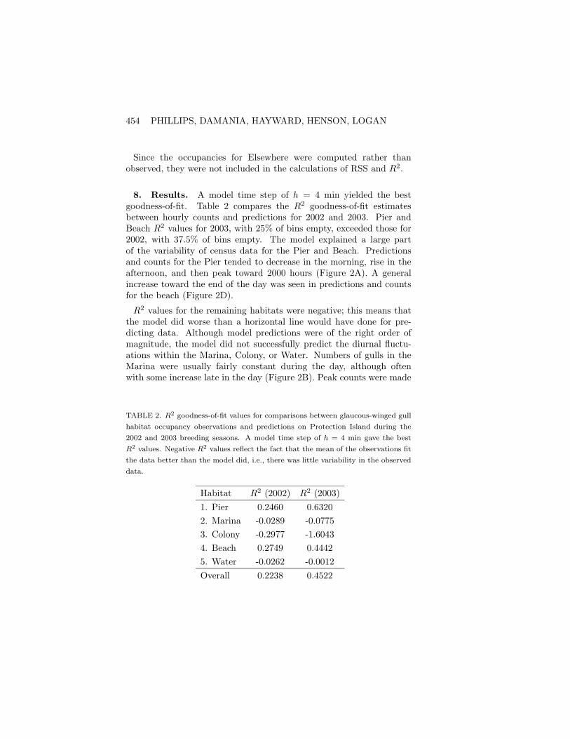
8. Results. A model time step of h = 4 min yielded the bestgoodness-of-fit. Table 2 compares the R2 goodness-of-fit estimatesbetween hourly counts and predictions for 2002 and 2003. Pier andBeach R2 values for 2003, with 25% of bins empty, exceeded those for2002, with 37.5% of bins empty. The model explained a large partof the variability of census data for the Pier and Beach. Predictionsand counts for the Pier tended to decrease in the morning, rise in theafternoon, and then peak toward 2000 hours (Figure 2A). A generalincrease toward the end of the day was seen in predictions and countsfor the beach (Figure 2D).

R2 values for the remaining habitats were negative; this means thatthe model did worse than a horizontal line would have done for pre-dicting data. Although model predictions were of the right order ofmagnitude, the model did not successfully predict the diurnal fluctu-ations within the Marina, Colony, or Water. Numbers of gulls in theMarina were usually fairly constant during the day, although oftenwith some increase late in the day (Figure 2B). Peak counts were made

TABLE 2. R2 goodness-of-fit values for comparisons between glaucous-winged gull

habitat occupancy observations and predictions on Protection Island during the

2002 and 2003 breeding seasons. A model time step of h = 4 min gave the best

R2 values. Negative R2 values reflect the fact that the mean of the observations fit

the data better than the model did, i.e., there was little variability in the observed

data.

Habitat R2 (2002) R2 (2003)1. Pier 0.2460 0.63202. Marina -0.0289 -0.07753. Colony -0.2977 -1.60434. Beach 0.2749 0.44425. Water -0.0262 -0.0012Overall 0.2238 0.4522

175

A. PIER176 177 178 179 180 181 182 183

184 185 186 189 190

(184)

(191)

300

160

-10

(190)(189)

Hour

Num

ber

of g

ulls

(188)

(187)(185)(183)(182)(181)(177)(175) (176)

191

2100

FIGURES 2A 2F. One-step model predictions (black circles) of gull habitat occupancies, on andaround Protection Island, point matched against the observations (open circles) in relation to tide(line). Each panel represents one day of observation. Day of the year is noted at the top lefthandcorner of each panel, with days in 2003 shown in parentheses. The horizontal axis is the hour of theday, and the vertical axis is the number of birds in the habitat. Some observations in the Water ondays 176, 179, (177), and (191), exceeded the y-axis and are represented by crossed out circles. Thevertical scale for the tide curve is -1 to 3 m.

175

B. MARINA176 177 178 179 180 181 182 183

184 185 186 189 190

(184)

(191)

-10

130(190)(189)

Hour

Num

ber

of g

ulls

(188)

(187)(185)(183)(182)(181)(177)(175) (176)

191

300 2100

FIGURE 2B.

175

C. COLONY176 177 178 179 180 181 182 183

184 185 186 189 190

(184)

(191)

-10

50(190)(189)

Hour

(188)

Num

ber

of g

ulls

(187)(185)(183)(182)(181)(177)(175) (176)

191

300 2100

FIGURE 2C.

175

D. BEACH176 177 178 179 180 181 182 183

184 185 186 189 190

(184)

(191)

-10

400(190)(189)

Hour

Num

ber

of g

ulls

(188)

(187)(185)(183)(182)(181)(177)(175) (176)

191

300 2100

FIGURE 2D.

175

E. WATER176 177 178 179 180 181 182 183

184 185 186 189 190

(184)

(191)

-10

50(190)(189)

Hour

Num

ber

of g

ulls

(188)

(187)(185)(183)(182)(181)(177)(175) (176)

191

300 2100

FIGURE 2E.

175

F. ELSEWHERE176 177 178 179 180 181 182 183

184 185 186 189 190

(184)

(191)

-10

850(190)(189)

Hour

Num

ber

of g

ulls

(188)

(187)(185)(183)(182)(181)(177)(175) (176)

191

300 2100

FIGURE 2F.


during some midday hours when temperatures were highest. Numbersof gulls in the Colony showed little variability; generally there was aslight decrease in numbers during the middle of the day followed byan increase during the evening (Figure 2C). Except for peaks in themidday hours, predictions and counts for the Water were also ratherconstant (Figure 2E).

Model predictions and estimated “counts” for Elsewhere showed apeak in mid- to late morning, followed by a general decrease in theevening hours, an inverse relationship compared with other habitats(Figure 2F). Since the occupancies for Elsewhere were computed ratherthan observed, they were not included in the calculations of RSS andR2.

Statistical tests for behaviors (Phillips [2004]) showed that behaviorfrequencies differed significantly by habitat in both terrestrial andaquatic environments (Figure 3). The following behaviors were morecommon than expected: Pier Stand Rest, Stand Sleep and StandPreen; Colony Sit Upright, Sit Rest, Stand Upright, Stand Rest,Walk and Other; Beach Sit Sleep, Stand Preen, Walk and Other;Marina Float; Water Bathe, Drink and Preen.

9. Discussion. Short-term fluctuations in habitat occupancies arelikely to be driven by the functional needs of birds (DeWoskin [1980],Cody [1985], Walsberg [1985]). To carry out various behaviors such aspreening, feeding, and resting, etc., gulls need to be in appropriate envi-ronments (Cooke and Ross [1972], Wondolowski [2002]). For example,gulls tended to congregate in the Marina or Water on very warm daysto float, bathe, and preen, and presumably unload heat (Damania et al.[2005]). Gulls used the terrestrial habitats primarily for sleeping, sit-ting, standing, resting and/or preening behaviors, generally referred toas loafing (Henson et al. [2004]). Behaviors on the colony also includedthose associated with territorialism.

The Pier and Beach yielded the best goodness-of-fit R2 values, partlybecause these two habitats experienced large fluctuations in gull occu-pancies. A habitat with large fluctuations around its mean occupancywill have a higher R2 than a habitat with an equal model error RSSbut relatively constant occupancies. This is because a larger denomina-tor in equation (6) leads to a higher R2 value. The Marina, Colony, and


0

50

100Pier

Terrestrial

Marina

Aquatic

0

50

100 Colony Water

Bat

he

Drin

k

Floa

t

Pre

en

0

50

100

Sit

uprig

htS

it re

stS

it sl

eep

Std

. upr

ight

Std

. res

tS

td. s

leep

Std

. pre

enW

alk

Oth

er

Beach

Per

cent

of b

ehav

iors

in h

abita

t

χ2terrestrial = 1013.12, p < 0.0001

χ2aquatic = 144.34, p < 0.0001

FIGURE 3. Percentages of behaviors exhibited most frequently by glaucous-winged gulls in each habitat on and around Protection Island. The category“Other” included behaviors which accounted for less than 1% of those countedwithin that habitat. Chi-square analysis was used to test the hypothesisthat distributions of behaviors differed among habitats; expected values weredetermined under the assumption of identical distributions across habitats.Habitats in terrestrial and aquatic environments were analyzed separately.Behavior designations follow Phillips [2004, Table 1].

Water showed much less variability in counts, which led to correspond-ingly smaller R2 values.

Because the model made reasonable predictions for the censused habi-tats with large fluctuations in counts, the predictions for Elsewhere alsoshould have been reasonable. Indeed, the results show distinct “occu-


pancy” patterns for Elsewhere (Figure 2F) that make biological sense,even though occupancy data were not collected for that habitat. Themaximum “occupancy” in Elsewhere always coincided with the lowesttides, possibly as a result of increased food availability at low waterlevels in other locations, as demonstrated in other studies (Patterson[1965], Drent [1967], Galusha and Amlaner [1978], Wondolowski [2002],Henson et al. [2004]). At higher tides gulls were expected to be dis-tributed throughout the five non-Elsewhere habitats. Model predic-tions suggested such a trend.

Although counts showed a general relationship with trends in modelpredictions, considerable deviation occurred between the two. Thisdeviation might have been due to several factors:

i. Disturbance: Human disturbances occurred mainly on the Pierand Colony, whereas flyovers by Bald Eagles (Haliaeetus leucocephalus)commonly influenced all the habitats (Galusha and Hayward [2002]).Gulls often responded to eagle disturbances with cyclonic “panicflights” (Hayward et al. [1977a]).

ii. Environmental variables: Whereas time of day and tide appar-ently functioned as the primary driving forces for count fluctuationsin some habitats (Henson et al. [2004]), no doubt other factors alsowere involved. Additional weather variables, including temperature,wind speed and direction, rain, and humidity also could have influ-enced habitat selection. Flow to the Marina, for example, seemed tobe driven more by temperature than by time or tide (Damania et al.[2005]); hence, observations for this habitat showed considerable devia-tion from model predictions. Thus, studies of additional environmentalfactors beyond tide height and time of day are needed to more accu-rately predict gull habitat occupancies. Variables such as temperature,however, cannot be used to develop long-range predictions.

iii. Visibility: The number of boats moored at the Pier not onlyaltered visibility but also affected the area available for loafing. Al-though gulls on boats were excluded, higher numbers of gulls on thePier would be expected if boats were not present. Count inaccuraciesalso may have occurred due to limited visibility during poor lightingconditions such as during fog and low solar elevation.


iv. Sampling and binning: Sample times may not have been represen-tative of movement patterns across habitats. Calculated flow rates mayhave been biased due to greater or lesser flow during non-observationhours. Although data were collected at discrete time intervals muchshorter than the periods of the tidal and diurnal cycles (Hunt andSchneider [1987], Levin [1992], Silverman et al. [2001]), the scale onwhich flow rates were binned and averaged was nonetheless rathercoarse. Binning at a finer scale may have produced better predictions,but would have required considerably more data.

v. Low counts: Small numbers of departures during some observa-tion periods and small occupancies in some habitats undoubtedly gaverise to considerable error in estimates of many of the per capita flowrates. In particular, the Water generally showed the lowest occupancies(Figure 2E), making reasonable predictions for this habitat difficult.

vi. Density-dependence and nesting behavior: Although some percapita flow rates may have depended on the density of gulls in the originor destination habitats, the model did not take this into account. Unlikethe other habitats, the Colony consisted of defended territories. Colonydynamics were probably tied to breeding behaviors that may have beendriven by aggressive encounters or other factors beyond simply time ofday and tide height.

vii. Social facilitation: Gulls appeared to move to and from otherhabitats independently of other gulls, except during disturbances andwhen assembling into feeding groups. This possibility, however, remainsunconfirmed. Other studies have found that social facilitation doesplay a role in at least some movement patterns of gulls (Evans [1982],Wittenberger and Hunt [1985], Gotmark et al. [1986]).

Studies that closely tie mathematical models of diurnal distributionto field data are rare in the literature. Exceptions include the studyby Henson et al. [2004] described in the introduction, and a study byHayward et al. [2005] who developed a deterministic model to predictseal haul-out patterns at Protection Island. Hayward et al.’s bestmodel explained 40% of the variability in hourly haul-out censuses.Silverman et al. [2001] developed a stochastic model for the dynamics ofmixed species waterfowl aggregations that described migration betweentwo “Colonies” in a closed system. Finally, Damania et al. [2005],in a continuous-time companion paper to this study, used differential


equations based on environmental variables to model the dynamics ofgulls in the Protection Island system of habitats. The Damania etal. [2005] model greatly increased accuracy by including the effects oftemperature and solar elevation.

Mathematical models typically are tied to data using free constantscalled “parameters.” Parameters are estimated by fitting the model todata using statistical procedures appropriate for the kind of noise inthe system. All of the related studies mentioned above utilized modelparameterization techniques such as sequential least squares. It shouldbe emphasized that the model developed in this paper involved nofree parameters and no model fitting. Instead, the parameters wereestimated directly from observations of flow rates.

In this paper the matrix model could not be iterated indefinitely intothe future because some bins contained missing data. Data collectionplans for the future include provisions for filling in the “missing bins,”which will allow the model to be run for longer periods of time. Afuture paper will address the asymptotic dynamics as well as stochasticversions of the matrix model.

10. Conclusion. Results from this study suggest that gull move-ments on and around Protection Island are correlated with a variety ofenvironmental cues, especially time of day and tide height. This sug-gests that in some cases complicated fluctuations of animal abundancein the field are influenced by deterministic forces and can be mathemat-ically modeled. Successful development of models that predict animalmovements could lead, among other benefits, to safer scheduling at air-ports to reduce the chance of bird/aircraft collisions, improvements inpublic health measures to control the spread of animal vector-bornediseases, and better resource management policies.

Acknowledgments. We would like to thank Kevin Ryan and theU.S. Fish and Wildlife Service for their permission to work on Protec-tion Island National Wildlife Refuge, Walla Walla College Marine Sta-tion for logistical support, Joe Galusha, Bob Desharnais, Jim Cushing,and Brian Dennis for discussions, and all the members of the SeabirdEcology Team at Andrews University, for criticism and support. This


research was funded in part by a faculty grant from Andrews Universityand by National Science Foundation grant DMS 0314512.

REFERENCES

C.J. Amlaner and J.F. Stout [1978], Aggressive Communication by Larus glau-cescens. Part VI: Interactions of Territory Residents with a Remotely Controlled,Locomotory Model, Behaviour 66, 223 251.

Anonymous [1998], Evergreen Pacific Tide Guide 1999, Evergreen Pacific Publ.Ltd., Shoreline, WA.

D.A. Bell [1997], Hybridization and Reproductive Performance in Gulls of theLarus glaucescens-occidentalis Complex, Condor 99, 585 594.

T.G. Benton, C.T. Lapsley and A.P. Beckerman [2002], The Population Responseto Environmental Noise: Population Size, Variance and Correlation in an Experi-mental System, J. Animal Ecol. 71, 320 332.

O.N. Bjørnstad and B.T. Grenfell [2001], Noisy Clockwork: Time Series Analysisof Population Fluctuations in Animals, Science 293, 638 643.

M.L. Cody [1985], An Introduction to Habitat Selection in Birds, in HabitatSelection in Birds (M.L. Cody, ed.), Academic Press, Orlando, FL.

R.F. Costantino, J.M. Cushing, B. Dennis and R.A. Desharnais [1995], Exper-imentally Induced Transitions in the Dynamic Behavior of Insect Populations,Nature 375, 227 230.

R.F. Costantino, R.A. Desharnais, J.M. Cushing and B. Dennis [1997], ChaoticDynamics in an Insect Population, Science 275, 389 391.

F. Cooke and R.K. Ross [1972], Diurnal and Seasonal Activities of a Post-Breeding Population of Gulls in Southeastern Ontario, Wilson Bulletin 84, 164 172.

J.M. Cushing, R.F. Costantino, B. Dennis, R.A. Desharnais and S.M. Henson[1998], Nonlinear Population Dynamics: Models, Experiments, and Data, J. Theor.Biol. 194, 1 9.

J.M. Cushing, R.F. Costantino, B. Dennis, R.A. Desharnais and S.M. Henson[2003], Chaos in Ecology: Experimental Nonlinear Dynamics, Academic Press, SanDiego, CA.

S.P. Damania, K.W. Phillips, S.M. Henson and J.L. Hayward, [2005], HabitatPatch Occupancy Dynamics in Glaucous-Winged Gulls (Larus glaucescens) II: AContinuous-Time Model, Natur. Resource Modeling 18, 469 498.

B. Dennis, R.A. Desharnais, J.M. Cushing, S.M. Henson and R.F. Costantino[2001], Estimating Chaos and Complex Dynamics in an Insect Population, Ecol.Monographs 71, 277 303.

R. DeWoskin [1980], Heat Exchange Influence on Foraging Behavior in ZonotrichiaFlocks, Ecology 61, 30 36.

R.H. Drent [1967], Functional Aspects of Incubation in the Herring Gull (Larusargentatus Pont.), Behaviour Suppl. 17, 1 32.

R.M. Evans [1982], Foraging-Flock Recruitment at a Black-Billed Gull Colony:Implications for the Information Center Hypothesis, The Auk 99, 24 30.


G.F. Fussmann, S.P. Ellner, K.W. Shertzer and N.G. Hairston [2000], Crossingthe Hopf Bifurcation in a Live Predator-Prey System, Science 290, 1358 1360.

J.G. Galusha and C.J. Amlaner [1978], The Effects of Diurnal and Tidal Pe-riodicities in the Numbers and Activities of Herring Gulls Larus argentatus in aColony, Ibis 120, 322 328.

J.G. Galusha and R.L. Carter [1987], Do Adult Gulls Recognize Their OwnYoung? An Experimental Test, Stud. Avian Biol. 10, 75 79.

J.G. Galusha and J.L. Hayward [2002], Bald Eagle Activity at a Gull Colony andSeal Rookery on Protection Island, Washington, Northwest. Natural. 83, 23 25.

J.G. Galusha and J.F. Stout [1977], Aggressive Communication by Larus glaucescens.Part IV: Experiments on Visual Communication, Behaviour 62, 222 235.

F. Gotmark, D.W. Winkler and M. Anderson [1986], Flock-Feeding of Fish SchoolsIncreases Individual Success in Gulls, Nature 319, 589 591.

J.L. Hayward, W.H. Gillett, C.J. Amlaner and J.F. Stout [1977a], Predation onGulls by Bald Eagles in Washington, The Auk 94, 375.

J.L. Hayward, W.H. Gillett and J.F. Stout [1977b], Aggressive Communicationby Larus glaucescens. Part V: Orientation and Sequences of Behavior, Behaviour62, 236 276.

J.L. Hayward, S.M. Henson, C.J. Logan, C.R. Parris, M.W. Meyer and B. Dennis[2005], Predicting Numbers of Hauled-Out Harbour Seals: A Mathematical Model,J. Appl. Ecol. 42, 108 117.

S.M. Henson, R.F. Costantino, J.M. Cushing, R.A. Desharnais, B. Dennis andA.A. King [2001], Lattice Effects Observed in Chaotic Dynamics of ExperimentalPopulations, Science 294, 602 605.

S.M. Henson, J.L. Hayward, C.M. Burden, C.J. Logan and J.G. Galusha [2004],Predicting Dynamics of Aggregate Loafing Behavior in Glaucous-Winged Gulls(Larus glaucescens) at a Washington Colony, The Auk 121, 380 390.

H.S. Horn [1975], Markovian Properties of Forest Succession, in Ecology andEvolution of Communities (M.L. Cody and J.M. Diamond, eds.), Belknap Press ofHarvard Univ. Press, Cambridge, MA, pp. 196 211.

G.L. Hunt, Jr., and D.C. Schneider [1987], Scale-Dependent Processes in the Phys-ical and Biological Environment of Marine Birds, in Seabirds: Feeding, Ecology andRole in Marine Ecosystems (J.P. Croxall, ed.), Cambridge Univ. Press, Cambridge,pp. 7 41.

E. James-Veich and E.S. Booth [1954], Behavior and Life History of the Glaucous-Winged Gull, Dept. of Biological Sciences and the Biological Station, PublicationNo. 12, Walla Walla College, WA.

S.A. Levin [1992], The Problem of Pattern and Scale in Ecology, Ecology 73,1943 1967.

J.R. McAuliffe [1988], Markovian Dynamics of Simple and Complex Desert PlantCommunities, Amer. Natur. 131, 459 490.

I.J. Patterson [1965], Timing and Spacing of Broods in the Black-Headed GullLarus ridibundus L., Ibis 107, 433 459.


K.W. Phillips [2004], Habitat Patch Occupancy Dynamics of Glaucous-WingedGulls (Larus glaucescens): A Discrete-Time Model, M.S. Thesis, Biology Depart-ment, Andrews University, MI.

W.V. Reid [1987], The Cost of Reproduction in the Glaucous-Winged Gull,Oecologia 74, 458 467.

W.V. Reid [1988a], Age-Specific Patterns of Reproduction in the Glaucous-Winged Gull: Increased Effort with Age, Ecology 69, 1454 1465.

W.V. Reid [1988b], Fledging Success of Experimentally Enlarged Broods of theGlaucous-Winged Gull, Wilson Bull. 100, 476 482.

W.V. Reid [1988c], Population Dynamics of the Glaucous-Winged Gull, J.Wildlife Manage. 52, 763 770.

E.D. Silverman, M. Kot and E. Thompson [2001], Testing a Simple StochasticModel for the Dynamics of Waterfowl Aggregations, Oecologia 128, 608 617.

J.F. Stout [1975], Aggressive Communication by Larus glaucescens. Part III: De-scription of the Displays Related to Territorial Protection, Behaviour 55, 181 208.

J.F. Stout and M. Brass [1969], Aggressive Communication by Larus glaucescens.Part II: Visual Communication, Behaviour 34, 42 54.

J.F. Stout, C.R. Wilcox and L.E. Creitz [1969], Aggressive Communication byLarus glaucescens. Part I: Sound Communication, Behaviour 34, 29 41.

P. Turchin [1998], Quantitative Analysis of Movement: Measuring and ModelingPopulation Redistribution in Animals and Plants, Sinauer Assoc., Sunderland, MA.

K. Vermeer [1963], The Breeding Ecology of the Glaucous-Winged Gull (Larusglaucescens) on Mandarte Island, B.C. Occasional Papers of the British ColumbiaProvincial Museum 13, 1 104.

G.E. Walsberg [1985], Physiological Consequences of Microhabitat Selection, inHabitat Selection in Birds (M.L. Cody, ed.), Academic Press, Orlando, FL, pp.389 413.

U.W. Wilson [1977], Reproductive Biology and Activity of the Rhinocerus Aukleton Protection Island, Washington, M.S. Thesis, University of Washington.

J.F. Wittenberger and G.L. Hunt, Jr. [1985], The Adaptive Significance of Colo-niality in Birds, in Avian Biology (D.S. Farner, J.R. King and K.C. Parkes, eds.),Vol. 8, Academic Press, Orlando, FL, pp. 1 78.

L. Wondolowski [2002], Diurnal Activity Patterns of Wintering Gulls at Jug BayWetland Sanctuary, M.S. Thesis, Bard College, Annendale-on-Hudson, NY.

J.T. Wootton [2001], Prediction in Complex Communities: Analysis of Empiri-cally Derived Markov Models, Ecology 82, 580 598.

HABITAT PATCH OCCUPANCY DYNAMICS OF GLAUCOUS-WINGED GULLS ( I: A

Documents

Transcript of HABITAT PATCH OCCUPANCY DYNAMICS OF GLAUCOUS-WINGED GULLS ( I: A