Habitat Fragmentation and the Southern Brown Bandicoot

Habitat Fragmentation and the

Southern Brown Bandicoot Isoodon obesulus

at Multiple Spatial Scales

David James Paull (MA Adel.)

School of Physical, Environmental and Mathematical Sciences (Geography)

University College University of New South Wales

A thesis submitted in fulfilment

of the requirements for the degree of Doctor of Philosophy

December 2003

ii

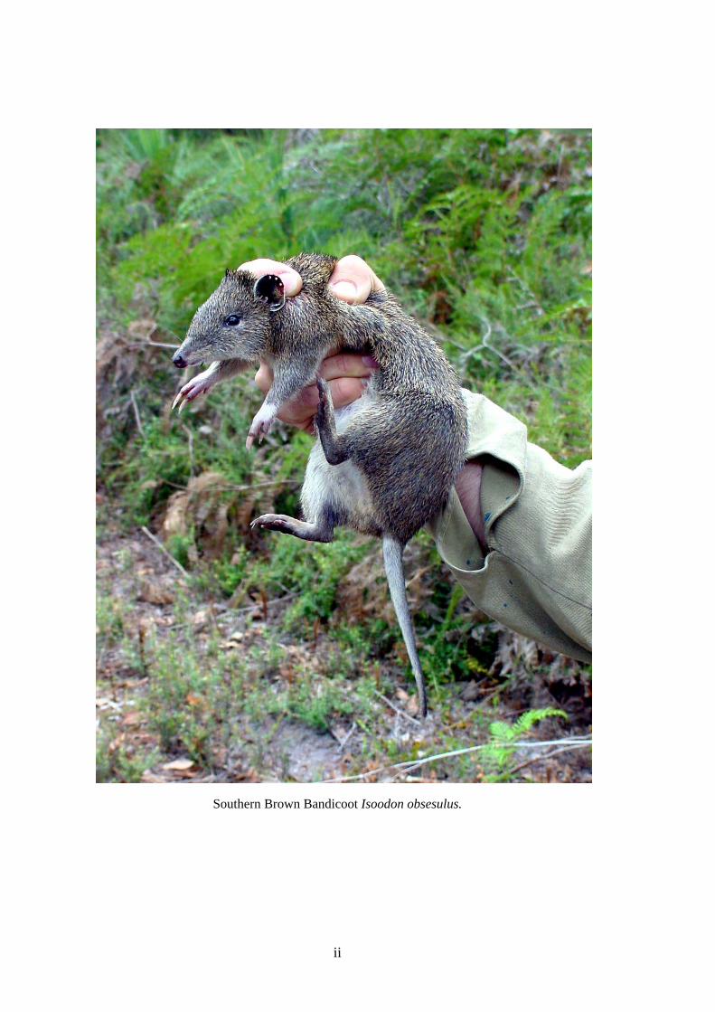
Southern Brown Bandicoot Isoodon obsesulus.

iii

CERTIFICATE OF ORIGINALITY

I hereby declare that this submission is my own work and to

the best of my knowledge it contains no materials

previously published or written by another person, nor

material which to a substantial extent has been accepted for

the award of any other degree or diploma at UNSW or any

other educational institution, except where due

acknowledgement is made in the thesis. Any contribution

made to the research by others, with whom I have worked at

UNSW or elsewhere, is explicitly acknowledged in the

thesis.

I also declare that the intellectual content of this

thesis is the product of my own work, except to the extent

that assistance from others in the project’s design and

conception or in style, presentation and linguistic

expression is acknowledged.

David James Paull

December 2003

v

ACKNOWLEDGEMENTS

This study was primarily carried out while I was a student of Geography in the School

of Geography and Oceanography, which in July 2003 was incorporated into the School

of Physical, Environmental and Mathematical Sciences. My supervisors were

Professor Dave Gillieson, Doctor Steve Morton and Professor Roger McLean, and

each was involved at critical stages of the research. Dave helped me to plan the topic

and played an important role in the development of the methodology presented in

Chapter 4. In the middle stages, Steve helped me to focus beyond the fieldwork phase

and to consider the place of my research within biogeography, landscape ecology and

conservation biology. Steve introduced me to colleagues at CSIRO including Nick

Nicholls, Peter Shaughnessy, Steve Cork and Dave Freudenberger who offered advice,

encouragement and support. Finally, Roger supervised while I wrote the thesis and he

was consistently helpful and patient. They all taught me much about research and

supervision of postgraduate students.

Staff from ForestrySA made important contributions. Barrie Grigg helped to

familiarized me with the study area in South Australia and his superb knowledge of

natural history was drawn upon during fieldwork. I am very grateful for the time he

spent validating fire records, identifying plants and pulling my vehicle out of bogs.

Peter Johnson and Brian Gepp of ForestrySA in Adelaide provided access to the nature

reserves studied and Des Kloeden of ForestrySA in Mt Gambier was immensely

helpful with GIS data. Mark Bachmann of the Department of Environment and

Heritage in Mt Gambier also gave great encouragement during the latter stages of the

study. Peter and Di Johnston and Wayne Cook joined me on two of the many

unforgettable field trips that I made to Mt Gambier. A big thank you goes to Dr Cathy

Robinson who helped me sieve hundreds of soil samples, especially considering soil

texture proved to be a significant variable. Cathy also offered critical reviews of

sections of the text.

Dr Andrew Claridge and Dr Doug Mills of the New South Wales National

Parks and Wildlife Service became great friends during the time that I worked on this

thesis and they provided balanced and useful feedback whenever I asked. Doug helped

with the Correspondence Analysis presented in Chapter 2 and Andrew with the

vi

BIOCLIM modelling. Thanks also go to my other great friend and colleague in

bandicoot studies, Michael Rees, who has contributed in important ways to this thesis

through the many discussions we have had about the topic. My employer, The

University of New South Wales, funded some of the travel expenses incurred during

fieldwork and the former School of Geography and Oceanography supplied maps,

computing and library resources. Ian McCredie prepared Figure 1.3, Ali Arezi took

care of all my computing requirements, Julie Kesby, Penny Umphelby and Christine

Kertesz searched for publications that were difficult to find and Peter Palmer helped

assemble equipment and prepare the vehicle for each field trip that I made. The

research was conducted under the University of New South Wales Animal Care and

Ethics Committee approval number ACE 96/118 and South Australian National Parks

and Wildlife Service permits numbered C08917-03 and Y10124-03.

vii

ABSTRACT

This thesis investigates the process of habitat fragmentation and the spatial and

temporal scales at which it occurs. Fragmentation has become an important topic in

biogeography and conservation biology because of the impacts it has upon species’

distributions and biodiversity. Various definitions of fragmentation are available but in

this research it is considered to be the disruption of continuity, either natural or

human-induced in its origins and operative at multiple spatial scales.

Using the distribution of the southern brown bandicoot Isoodon obesulus as a

case study, three spatial scales of fragmentation were analysed. At the continental

scale, the Australian distribution of the subspecies I. o. obesulus was examined in

relation to climate, geology and vegetation cover at the time of European settlement of

Australia and two centuries later. Using archived wildlife records and Geographic

Information Systems (GIS) analyses, habitat suitability models were created to assess

natural and human-induced fragmentation of the distribution of I. obesulus in 1788 and

1988. At the regional scale, a study was made of the distribution of I. obesulus in the

south-east of the State of South Australia. Again, natural and human-induced patterns

of habitat fragmentation were modelled using GIS with climate, soil and vegetation

data for the time of European settlement and at present. At the local scale, the

distribution of I. obesulus was the subject of a detailed field survey of 372 sites within

29 remnant patches of native vegetation in south-eastern South Australia in order to

understand the variables that cause habitat fragmentation. Geographic information

systems were used again but in a different way to carefully stratify the field survey by

overlaying maps of topography, vegetation and past fires. The large dataset collected

from the surveys was described using six generalized linear models which identified

the significant variables that fragment the distribution of I. obesulus at a local scale.

From the results of the field surveys, a subset of four remnants was chosen for further

GIS spatial modelling of the probability of I. obesulus occurring within remnants in

response to fire via a controlled burning programme put in place to reduce

accumulating fuel loads.

These investigations show that habitat fragmentation can be caused by different

factors at different spatial scales. At the continental scale, it was found that climate

viii

played a dominant role in influencing the fragmented distribution of I. obesulus but

vegetation change during the past two centuries has also had a profound impact on the

availability of habitat. Within south-eastern South Australia, the species’ regional scale

distribution is constrained by climate and also by soil and vegetation patterns.

Dramatic change to its regional distribution occurred in the 20th century as a result of

the clearance of native vegetation for planting pastures, crops and pines.

Fragmentation at the regional scale has resulted in the remaining habitat being reduced

to small, isolated, remnant patches of native vegetation. At the local scale it was found

that variables which disrupt the continuity of I. obesulus habitat within remnants

include vegetation cover in the 0-1 m stratum, abundance of Xanthorrhoea australis

and soil texture. For a subset of sites located in one landsystem of the study area,

named Young, the age of vegetation since it was last burnt was also found to be a

significant variable, with vegetation 10-14 years old since burning providing the most

suitable habitat. Spatial modelling of two scenarios for prescribed burning over 15

years revealed that the use of fire as a habitat enhancement tool will be complicated

and require a detailed understanding of the factors that cause natural fragmentation in

the distribution of I. obesulus at the local scale.

A further conclusion of the study was that ecological relationships between

species and their habitats require careful interpretation of multi-scaled datasets and

conservation plans for endangered species ought to be made at multiple spatial scales.

Future research directions are identified including the linking of multi-scaled habitat

fragmentation models to genetic studies of the species throughout its range.

ix

TABLE OF CONTENTS

FRONTISPIECE……………………………………………………………………………………...…ii

CERTIFICATE OF ORIGINALITY ................................................................................................... iii

ACKNOWLEDGEMENTS .................................................................................................................... v

ABSTRACT ........................................................................................................................................ vii

TABLE OF CONTENTS ....................................................................................................................... ix

LIST OF FIGURES.............................................................................................................................. xiii

LIST OF TABLES................................................................................................................................. xv

CHAPTER 1. FRAGMENTATION AND THE SOUTHERN BROWN BANDICOOT.................. 1

1.1 THE CONCEPT OF FRAGMENTATION............................................................................................. 1

1.2 SPECIES’ DISTRIBUTIONS AND SPATIAL SCALES .......................................................................... 2

1.3 THE SOUTHERN BROWN BANDICOOT........................................................................................... 6

1.3.1 Biology and Ecology.......................................................................................................... 6

1.3.2 Distribution and Taxonomy ............................................................................................... 7

1.3.3 Conservation Status......................................................................................................... 10

1.4 SECTIONS OF THE THESIS ........................................................................................................... 13

CHAPTER 2. CONTINENTAL SCALE DISTRIBUTION OF ISOODON OBESULUS............... 15

2.1 MODELLING THE DISTRIBUTION OF SPECIES .............................................................................. 15

2.2 METHODS................................................................................................................................... 16

2.2.1 Bioclimatic Modelling ..................................................................................................... 17

2.2.2 Climate Suitability Mapping............................................................................................ 22

2.2.3 Geologic Suitability Mapping.......................................................................................... 22

2.2.4 Vegetation Suitability Mapping ....................................................................................... 24

2.2.5 Habitat Suitability Mapping ............................................................................................ 26

2.2.6 Model Validation ............................................................................................................. 27

2.3 RESULTS .................................................................................................................................... 28

2.3.1 Climate Suitability ........................................................................................................... 28

2.3.2 Geologic Suitability ......................................................................................................... 31

2.3.3 Vegetation Suitability in 1788 and 1988 ......................................................................... 34

2.3.4 Habitat Suitability in 1788 and 1988 .............................................................................. 38

2.3.5 Climatic Difference between Regions.............................................................................. 40

x

2.4 DISCUSSION................................................................................................................................44

2.4.1 Distribution and Fragmentation of Isoodon obesulus .....................................................44

2.4.2 Influence of Climate, Geology and Vegetation ................................................................45

CHAPTER 3. REGIONAL SCALE DISTRIBUTION OF ISOODON OBESULUS .......................47

3.1 ISOODON OBESULUS IN THE SOUTH EAST OF SOUTH AUSTRALIA ................................................47

3.1.1 The Study Area .................................................................................................................50

3.2 METHODS ...................................................................................................................................60

3.2.1 Selection of Modelling Records .......................................................................................60

3.2.2 Climate Suitability............................................................................................................61

3.2.3 Soil Suitability Classification ...........................................................................................61

3.2.4 Vegetation Suitability Classification................................................................................62

3.2.5 Pre-European and Present Habitat Suitability Mapping.................................................62

3.3 RESULTS.....................................................................................................................................63

3.3.1 Climate Suitability............................................................................................................63

3.3.2 Soil Suitability ..................................................................................................................64

3.3.3 Vegetation Suitability .......................................................................................................68

3.3.4 Habitat Suitability ............................................................................................................72

3.4 DISCUSSION................................................................................................................................76

CHAPTER 4. LOCAL SCALE I. HABITAT USE IN THE SOUTH EAST.................................... 79

4.1 INTRODUCTION...........................................................................................................................79

4.1.1 Habitat Suitability at the Local Scale ..............................................................................79

4.2 METHODS ...................................................................................................................................83

4.2.1 Statification of Sampling Units ........................................................................................84

4.2.2 Field-based Site Surveys ..................................................................................................90

4.2.3 Statistical Analysis ...........................................................................................................96

4.3 RESULTS.....................................................................................................................................97

4.3.1 Distribution and Abundance of Diggings ........................................................................97

4.3.2 Assessment of Sampling ...................................................................................................99

4.3.3 The Response and Explanatory Variables .....................................................................101

4.3.4 Generalized Linear Modelling .......................................................................................109

4.4 DISCUSSION..............................................................................................................................115

4.4.1 Distribution and Abundance of Diggings ......................................................................115

4.4.2 Sampling Methods..........................................................................................................115

4.4.3 Variables and Models .................................................................................................... 117

4.4.4 Local Scale Fragmentation and Implications for Habitat Management .......................119

xi

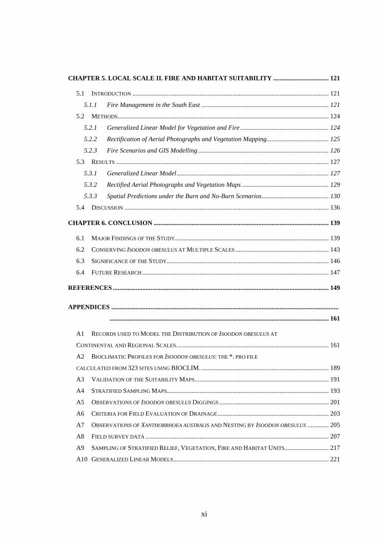
CHAPTER 5. LOCAL SCALE II. FIRE AND HABITAT SUITABILITY .................................. 121

5.1 INTRODUCTION ........................................................................................................................ 121

5.1.1 Fire Management in the South East .............................................................................. 121

5.2 METHODS................................................................................................................................. 124

5.2.1 Generalized Linear Model for Vegetation and Fire ...................................................... 124

5.2.2 Rectification of Aerial Photographs and Vegetation Mapping...................................... 125

5.2.3 Fire Scenarios and GIS Modelling ................................................................................ 126

5.3 RESULTS .................................................................................................................................. 127

5.3.1 Generalized Linear Model............................................................................................. 127

5.3.2 Rectified Aerial Photographs and Vegetation Maps ..................................................... 129

5.3.3 Spatial Predictions under the Burn and No-Burn Scenarios......................................... 130

5.4 DISCUSSION ............................................................................................................................. 136

CHAPTER 6. CONCLUSION ........................................................................................................... 139

6.1 MAJOR FINDINGS OF THE STUDY.............................................................................................. 139

6.2 CONSERVING ISOODON OBESULUS AT MULTIPLE SCALES ......................................................... 143

6.3 SIGNIFICANCE OF THE STUDY................................................................................................... 146

6.4 FUTURE RESEARCH .................................................................................................................. 147

REFERENCES .................................................................................................................................... 149

APPENDICES ...........................................................................................................................................

...................................................................................................................................... 161

A1 RECORDS USED TO MODEL THE DISTRIBUTION OF ISOODON OBESULUS AT

CONTINENTAL AND REGIONAL SCALES. ............................................................................................ 161

A2 BIOCLIMATIC PROFILES FOR ISOODON OBESULUS: THE *. PRO FILE

CALCULATED FROM 323 SITES USING BIOCLIM. .............................................................................. 189

A3 VALIDATION OF THE SUITABILITY MAPS.................................................................................. 191

A4 STRATIFIED SAMPLING MAPS................................................................................................... 193

A5 OBSERVATIONS OF ISOODON OBESULUS DIGGINGS ................................................................... 201

A6 CRITERIA FOR FIELD EVALUATION OF DRAINAGE.................................................................... 203

A7 OBSERVATIONS OF XANTHORRHOEA AUSTRALIS AND NESTING BY ISOODON OBESULUS ............. 205

A8 FIELD SURVEY DATA ................................................................................................................ 207

A9 SAMPLING OF STRATIFIED RELIEF, VEGETATION, FIRE AND HABITAT UNITS........................... 217

A10 GENERALIZED LINEAR MODELS............................................................................................... 221

xiii

LIST OF FIGURES 1.1 Land transformation processes, including fragmentation. 2

1.2 Illustrations of Isoodon obesulus. 6

1.3 Distribution of Isoodon obesulus at the continental scale. 8

2.1 Occurrence records attributed to Isoodon obesulus. 19

2.2 Records used to model and validate the distribution of Isoodon obesulus at a continental scale. 19

2.3 Lithological Association and Regolith Class of the study area. 23

2.4 Vegetation of the study area in 1788 and 1988. 25

2.5 BIOMAP outputs and the climate suitability map. 30

2.6 Geologic suitability maps. 33

2.7 Vegetation suitability for Isoodon obesulus in 1788 and 1988. 37

2.8 Habitat suitability for Isoodon obesulus in 1788 and 1988. 38

2.9 Cluster Analysis of BIOCLIM profiles for regions inhabited by Isoodon obesulus. 42

2.10 Correspondence Analysis of BIOCLIM profiles for regions inhabited by Isoodon obesulus. 43

3.1 The South East of South Australia with historical records of Isoodon obesulus. 48

3.2 Remnant native vegetation associated with accurate and reliable records of Isoodon obesulus. 49

3.3 Annual mean rainfall and temperature of the South East. 50

3.4 Physiographic and geological features of the South East. 52

3.5 Soil Groups of the South East. 55

3.6 Pre-European vegetation of the South East. 58

3.7 Present native vegetation of the South East. 59

3.8 Records used to model the distribution of Isoodon obesulus at a regional scale. 60

3.9 Suitability of climate for Isoodon obesulus in the South East. 63

3.10 Suitability of soil for Isoodon obesulus in the South East. 67

3.11 Suitability of pre-European and present vegetation for Isoodon obesulus in the South East. 72

3.12 Suitability of pre-European and present habitat for Isoodon obesulus in the South East. 73

3.13 Change to the area of habitat suitability in the South East. 74

xiv

3.14 Change to the distribution of pre-European habitat suitability in the South East. 75

4.1 Typical conical digging of Isoodon obesulus. 81

4.2 Nest of Isoodon obesulus. 81

4.3 Patches of remnant native vegetation surveyed in the South East. 83

4.4 Construction of digital elevation models and stratification of local relief. 86

4.5 Vegetation sampling units for Woolwash. 87

4.6 Fire sampling units for Woolwash. 88

4.7 Habitat sampling units for Woolwash and site locations. 89

4.8 Quadrat dimension and active search pattern. 90

4.9 Distribution and abundance of Isoodon obesulus diggings at 372 sites in 1998/99. 98

4.10 Assessment of sampling of habitat units. 100

4.11 Frequency of sites in digging abundance classes. 101

4.12 Abundance of diggings in response to relief, landform, drainage and soil. 102

4.13 Abundance of diggings in response to vegetation structure. 104

4.14 Abundance of diggings in response to vegetation composition. 106

4.15 Abundance of diggings in response to fire. 107

4.16 Abundance of diggings in response to ground surface characteristics. 108

5.1 Age of fire management blocks since last burning and dates of proposed fires. 123

5.2 Effect of fire on Xanthorrhoea australis. 123

5.3 Ground control points used to rectify aerial photographs. 126

5.4 Rectified aerial photographs of remnants in the Young landsystem. 129

5.5 Vegetation classification of remnants in the Young landsystem. 130

5.6 Probability of diggings occurring under the burn scenario. 133

5.7 Probability of diggings occurring under the no-burn scenario. 134

5.8 Probability of diggings occurring in remnants, by area. 135

6.1 Fragmentation of Isoodon obesulus habitat at multiple spatial and temporal scales. 139

xv

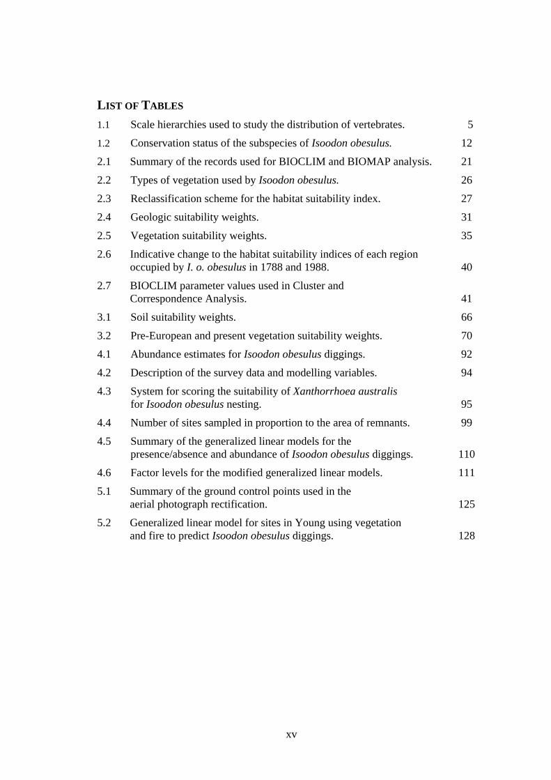
LIST OF TABLES 1.1 Scale hierarchies used to study the distribution of vertebrates. 5

1.2 Conservation status of the subspecies of Isoodon obesulus. 12

2.1 Summary of the records used for BIOCLIM and BIOMAP analysis. 21

2.2 Types of vegetation used by Isoodon obesulus. 26

2.3 Reclassification scheme for the habitat suitability index. 27

2.4 Geologic suitability weights. 31

2.5 Vegetation suitability weights. 35

2.6 Indicative change to the habitat suitability indices of each region occupied by I. o. obesulus in 1788 and 1988. 40

2.7 BIOCLIM parameter values used in Cluster and Correspondence Analysis. 41

3.1 Soil suitability weights. 66

3.2 Pre-European and present vegetation suitability weights. 70

4.1 Abundance estimates for Isoodon obesulus diggings. 92

4.2 Description of the survey data and modelling variables. 94

4.3 System for scoring the suitability of Xanthorrhoea australis for Isoodon obesulus nesting. 95

4.4 Number of sites sampled in proportion to the area of remnants. 99

4.5 Summary of the generalized linear models for the presence/absence and abundance of Isoodon obesulus diggings. 110

4.6 Factor levels for the modified generalized linear models. 111

5.1 Summary of the ground control points used in the aerial photograph rectification. 125

5.2 Generalized linear model for sites in Young using vegetation and fire to predict Isoodon obesulus diggings. 128

1

CHAPTER 1 FRAGMENTATION AND THE SOUTHERN BROWN BANDICOOT

This thesis is concerned with the distribution of the southern brown bandicoot at

multiple spatial scales ranging from the continental to the local. The southern brown

bandicoot is a small Australian marsupial, which although once widespread now has

a limited distribution and has recently been listed as an endangered species under the

Australian Environmental Protection and Biodiversity Conservation Act 1999. Since

European settlement, the continuity of the animal’s habitat has been disrupted

resulting in a fragmented distribution. Thus, critical to the analysis presented here is

the concept of habitat fragmentation.

1.1 The Concept of Fragmentation

Fragmentation became a key concept in conservation biology during the 1980s and it

is normally used when referring to the processes that lead to “the breaking up of

habitat or land type into smaller parcels” (Forman 1995 p 408). Fragmentation is “the

progressive division of a larger habitat into smaller pieces…with increasing isolation

and, in many cases, decreasing independent viability” (New 2000 p 372). The spatial

pattern that results from fragmentation can be visualized as a broken dinner plate

(Figure 1.1) but the fragments of habitat are not scattered, as would be those from a

dropped plate, instead they are remnants (Forman 1995). Habitat fragmentation can

result from the land transformation processes of perforation and dissection, and it

precedes shrinkage and attrition (Forman 1995). Perhaps the simplest definition of

fragmentation, and the one adopted in this thesis, is “the disruption of continuity”

(Lord and Norton 1990 p 197).

Habitat fragmentation has been described variously as being “the man-made

change imposed on natural habitat heterogeneity” (Caughley and Gunn 1996 p 242)

and either human-induced or natural in its origins (Forman 1995, Lord and Norton

1990). Bleich et al. (1990 p 383), for example, described the habitat of mountain

sheep Ovis canadensis in southern California as being “naturally fragmented” by

topographic features. Other studies have focussed on the biotic effects of human-

2

induced habitat fragmentation resulting from vegetation clearance (Harris 1984) and

found that the major consequences for biota are loss of habitat, increased isolation of

habitat remnants and greater exposure to edge effects (Haila et al. 1993, New 2000).

Rees and Paull (2000) concluded that human-induced patterns of habitat

fragmentation are imprinted over natural fragmentation patterns and they jointly

influence the distribution of species.

1.2 Species’ Distributions and Spatial Scales

The distribution of species is tied to the distribution of suitable habitat, so

fragmentation impacts negatively on species that depend on large areas of intact

habitat. Miller (2000) observed that habitat is not a synonym for vegetation because

the latter is a collective term for plants, while habitat is a species-specific concept

that can be defined as “an area with the combination of resources (like food, cover,

water) and environmental conditions (temperature, precipitation, presence or absence

of predators and competitors) that promotes occupancy by individuals of a given

species (or population) and allows those individuals to survive and reproduce”

Perforation

Fragmentation

Dissection

Shrinkage

Attrition

Figure 1.1 Land transformation processes, including fragmentation.

Adapted from Forman 1995 Fig 12.1 p 407.

3

(Morrison et al. 1992 cited in Miller 2000).

The continuity of habitats and thus species’ distributions can be fragmented at

multiple scales. Recent studies have emphasized the importance of considering

multiple spatial scales when analysing wildlife distributions because the factors that

affect species’ distributions may not be apparent at a single scale (Bissonette 1997,

Bissonette et al. 1997, Fauchald et al. 2000, Lindenmayer 2000, Storch 1997, Wiens

1989). Resources and environmental factors change at multiple spatial scales

(Mackey and Lindenmayer 2001) and the distributions of species change at

commensurate spatial scales. The value of examining wildlife habitat over large

areas, therefore, lies in understanding the broad scale constraints that may be

imposed on individual animals at finer scales (Bissonette et al. 1997).

When considering the distribution of species, it is appropriate to consider a

nested hierarchy of interdependent spatial scales. Analyses conducted at only one

spatial scale may limit the understanding of ecological relationships and do not

reflect the hierarchical way that organisms respond to the distribution of their habitat

(Bissonette et al. 1997, Wiens 1989). Most fragmentation studies have focussed on a

single spatial scale, particularly the patch scale (Haila 2002) but habitat

fragmentation occurs at multiple scales. Lord and Norton (1990) asserted that the

concept of fragmentation can be applied at a range of scales across spatial, temporal

and functional domains, and illustrated this point with the example of grassland

fragmentation at two spatial scales. The first of these was termed by Lord and Norton

(1990) geographic fragmentation, which is synonymous with landscape scale

fragmentation of forest and woodland vegetation into remnant patches. The second

was structural fragmentation, which was applied to fine scale invasion of inter-

tussock swards by exotic grasses in New Zealand native grasslands. Lord and Norton

(1990 p 197) showed that because “ecosystems function across a wide range of

spatial scales, fragmentation is not scale-limited”. This is an important point because

it potentially makes the term habitat modification redundant by introducing “the

concept of a continuum of spatial scales of destruction” (McIntyre and Hobbs 1999 p

1286). In this thesis, it will be shown that habitat fragmentation does occur at

multiple spatial scales including additional, broader scales to structural

fragmentation and geographic fragmentation.

4

Processes such as climatic and geologic change operating over long time

scales can fragment the broad scale distribution of species. For example, it is

believed that the continental distribution of the oligostenothermic mountain pygmy

possum (Burramys parvus) became fragmented by change to the thermocline after

the last glacial maximum (Broome and Mansergh 1989). At successively finer scales

relatively fast-acting processes that lead to geomorphic, pedologic and vegetation

change, and therefore habitat change, may fragment the distributions of subspecies

and populations.

The relevant scales for analysing the distribution of species are not easily

defined. Cale and Hobbs (1994 p 183) considered, “scales of study have to match the

scale of processes in which we are interested, or the scale at which particular

organisms perceive their environment.” Individual animals respond to their

environment at multiple spatial scales with the smallest area corresponding to the

smallest objects they perceive and the largest area being the home range (Kotliar and

Wiens 1990). Studies of the distribution of vertebrates at multiple spatial scales have

been conducted before and examples include leadbeaters possum Gymnobelideus

leadbeateri, the capercaillie Tetrao urogallus and the American marten Martes

americana. In the case of G. leadbeateri, Lindenmayer (2000) demonstrated that the

factors which influence its distribution should be examined over a range of spatial

scales and the results integrated into conservation plans. Storch (1997) analysed the

distribution of T. urogallus at the continental scale, the regional scale, the local scale

and the forest stand scale (Table 1.1), and concluded that the long-term survival of

the species depended on the availability of habitats at all scales. When examining the

distribution of M. americana, Bissonette et al. (1997) defined four spatial scales,

being the landscape scale, the home range scale, the stand scale and the microhabitat

scale. In an attempt to establish a generic framework for analysing the distribution of

species, Mackey and Lindenmayer (2001) proposed a five-level environmental

hierarchy based on five scales at which resources are distributed, termed the global,

meso, topo, micro and nano scales. Clearly there are many ways to describe scales

but in the present study three spatial scales are used to investigate the fragmented

distribution of the southern brown bandicoot Isoodon obesulus. They are termed the

continental, regional and local scales and they correspond to the subspecies’

5

distribution in Australia, in the south-east region of South Australia and within

remnant patches of native vegetation in that region.

Table 1.1 Scale hierarchies used to study the distribution of vertebrates.

Lindenmayer (2000) Gymnobelideus leadbeateri

Storch (1997) Tetrao urogallus

Bissonette et al. (1997) Martes americana

Mackey and Lindenmayer (2001) Generic framework

Global - boreal forests of Siberia and Fennoscandia

Global - latitude and seasonal variation in extra-terrestrial radiation

Broad scale - bioclimatic distribution

Continental - montane conifer forests in Central Europe

Meso - weather systems, topographic elevation and substrate lithology

Regional - forested mountain ranges

Topo - local topography, slope, aspect and radiation

Landscape - patches and corridors in timber harvesting areas

Landscape - percentage of forest cover

Home Range - age of forest stands

Local - age of forest stands on mountain range

Stand - forest structural attributes

Stand - canopy cover and ground vegetation

Stand - vegetation structure and species compostion

Micro - vegetation structure and availability of coarse woody debris

Micro - impact of forest canopy on below-canopy soil moisture and nutrients

Tree - availability of den sites

Nano - vegetation layering, woody biomass, soil mico-organisms, distribution of water and nutrients

6

1.3 The Southern Brown Bandicoot

1.3.1 Biology and Ecology

The southern brown bandicoot Isoodon obesulus is a small ground-dwelling

Australian marsupial that occurs in southern and eastern Australia. It can be

recognised by its elongated muzzle, small round ears and short tail (Figure 1.2).

Males weigh an average of 850 g and females 700 g (Braithwaite 1983). Its fur has a

brown, grizzled appearance due to a combination of black outer guard hairs and soft

yellowish grey to pale grey underfur (Jones 1924). The forelimbs are short relative to

the hindlimbs and they have strong flattened foreclaws that are well adapted for

digging in the upper soil horizons (Gordon and Hulbert 1989). There is a syndactylus

fusion of the second and third digits of the pes, which is a characteristic of

herbivorous marsupials; however, I. obesulus is an omnivore with a dental formula

of I5/3, C1/1, P3/3, M4/4. Its dietary preference is for subterranean invertebrates,

especially Coleoptera but including Acarina, Annelida, Arachnida, Chilopoda,

Collembola, Dermaptera, Diptera, Hemiptera, Hymenoptera, Isopoda, Lepidoptera,

Orthoptera and Siphonaptera (Jones 1924, Heinsohn 1966, Opie 1980, Quin 1985a,

1985b, Watts 1974). Subterranean sporocarps of hypogeous fungi also constitute an

important part of its diet (Claridge 1988, Claridge et al. 1991) and minor food items

eaten opportunistically by I. obesulus include plant material and small vertebrates,

for example skinks and frogs (Heinsohn 1966).

Figure 1.2 Illustrations of Isoodon obesulus. Adapted from Jones (1924), Figs 93, 94 and 95.

7

The vegetation types inhabited by I. obesulus include native forests,

woodlands, shrublands, heathlands and sedgelands (Braithwaite 1983, Braithwaite

and Gullen 1978, Lobert 1985, Lobert and Lee 1990, Lobert and Opie 1986,

Menkhorst and Beardsell 1982, Moro 1991, Opie 1980, Opie et al. 1990, Paull 1993,

Rees 1997, Stoddart and Braithwaite 1979, Wilson et al. 1990). In some instances,

the species has been reported from exotic vegetation including boxthorn (Heinsohn

1966) and blackberries (Paull 1993) but only in areas where native vegetation also

exists. There is substantial inter-regional and intra-regional variation in the types of

vegetation used by I. obesulus but some common elements are displayed, for

example, dense ground cover that provides shelter from predators (Heinsohn 1966,

Paull 1995).

1.3.2 Distribution and Taxonomy

The distribution of I. obesulus is fragmented at multiple spatial scales. At a

continental scale, the species exists as a series of regional populations scattered

across the coastal margins of southern and eastern Australia, between south-western

Western Australia and Cape York Peninsula in Queensland (Figure 1.3). Throughout

this range, five subspecies are recognized, based on morphological variations in body

size, pelage, cranial dimensions and dental features (Seebeck et al. 1990). The

subspecies Isoodon obesulus obesulus, which is the subject of this thesis, occurs in

southern South Australia, southern Victoria and eastern New South Wales with a

northern limit at the Hawkesbury River (Dixon 1978). Its relatives occur in far north

Queensland (I. o. peninsulae), in Tasmania (I. o. affinis), on islands of Nuyts

Archipelago in the Great Australian Bight (I. o. nauticus) and in south-western

Western Australia (I. o. fusciventer).

Uncertainty exists about these taxonomic groups. Based on cranial

characteristics, Dixon and Huxley (1985) considered that I. o. peninsulae was a

subspecies of I. obesulus but Gordon and Hulbert (1989) suggested that it may be

part of the Golden Bandicoot (Isoodon auratus) group. Jones (1924), Troughton

(1973) and Lyne and Mort (1981) viewed I. o. peninsulae and I. o. nauticus as being

distinct species to I. obesulus but Braithwaite (1983) did not recognize I. o. nauticus

and thought that I. o. affinis may be an invalid subspecies. Genetic studies have

8

provided information on the relationships between populations of I. obesulus in

different geographic locations. In an electrophoretic and chromosome survey of the

genus Isoodon, Close et al. (1990) found that I. o. peninsulae was the most distinct

taxon of the I. obesulus group and that I. o. obesulus from New South Wales and

Victoria were similar to I. o. affinis. Pope et al. (2001) reached the same conclusion

about the distinctive genetic character of I. o. peninsulae. Isoodon o. obesulus from

the Mount Lofty Ranges in South Australia has been found to align genetically with

I. o. fusciventer and I. o. nauticus, which suggests that the contact zone for I. o.

obesulus and I. o. fusciventer lies between Adelaide and Melbourne, not Adelaide

and Perth as shown in Figure 1.3 (Close et al. 1990). This finding was supported by

Adams (in Maxwell et al. 1996 p 7) who detected genetic variation in I. obesulus

east and west of the lower Murray River valley. Despite the uncertainty about

taxonomic relationships between I. obesulus in different geographic locations, the

present study will adhere to the classification of Seebeck et al. (1990), which is

shown in Figure 1.3.

Figure 1.3 Distribution of Isoodon obesulus at the continental scale.

Adapted from Rees and Paull (2000) and Pope et al. (2001). Originally compiled by Rees and Paull (2000) from Ashby et al. (1990), Friend (1990), Gordon et al. (1990), Hocking (1990), Kemper (1990), Menkhorst and Seebeck (1990), Paull (1995).

9

The importance of a taxonomic discussion for the present study, which

emphasizes the subspecies I. o. obesulus, is that the close relationships between

relatives in widely separated regions help to explain how the species’ distribution

became fragmented and why it currently exists as a series of widely dispersed

subspecies and regional populations. Pope et al. (2001 p 425) observed that “the

levels of genetic divergence among populations of I. obesulus and I. auratus are

sufficiently low to support the idea that there was once a single, geographically

continuous species across most of Australia that has in recent times suffered range

reduction and subsequent population isolation.” Close et al. (1990) also proposed the

theory that a recent interruption to gene flow occurred between geographically

distant populations of I. obesulus.

If I. obesulus did once have a continuous distribution across Australia, then it

is probable that genetic variation occurred throughout its range prior to the

development of the fragmented continental scale distribution seen in Figure 1.3. It

can be assumed that post-glacial sea level rise fragmented I. o. affinis on Tasmania

and I. o. nauticus on Nuyts Archipelago from the mainland. This subspeciation could

have occurred in times as recent as the late Pleistocene - early Holocene as a

consequence of sea level rise (Yokohama et al. 2001).

The fragmentation of three mainland subspecies is more complex. If I.

obesulus had a near-coastal or peripheral continental distribution during the late

Pleistocene, as it currently does, then extensive areas of habitat that once linked I. o.

peninsulae, I. o. obesulus and I. o. fusciventer may have been lost as a result of sea

level rise in the early Holocene. Alternatively, if the species occupied more inland

parts of Australia, increasing aridity in the late Pleistocene may have forced its

distribution outward towards a shrinking continental margin in the Holocene. Gordon

and Hulbert (1989 p 616) observed that the “broad patterns of distribution [of

Australian peramelids] are determined particularly by climatic factors, such as

rainfall gradients”. Today, a significant climatic disjunction between the tropical and

subtropical/temperate zones of eastern Australia fragments I. o. peninsulae from I. o.

obesulus by a distance of approximately 2000 km. In southern Australia, the arid

Nullarbor Plain and northern Eyre Peninsula fragment I. o. fusciventer from I. o.

obesulus by a distance of approximately 1500 km.

10

Within the distributions of the five I. obesulus subspecies further

fragmentation exists (Figure 1.3). In some situations naturally occurring geographic

features are evident, for example the lower Murray River valley and Coorong region

of South Australia correspond with a disjunction in the distribution of I. o. obesulus

(Figure 1.3). In other situations, land cover changes brought about by humans have

caused habitat loss particularly due to the clearance of native vegetation. This is most

noticeable from the reduced distribution of I. o. fusciventer in the wheatbelt region of

Western Australia (Friend 1990).

One possibility that is not investigated in this thesis is that Aboriginal people

influenced the fragmented distribution of I. obesulus prior to European settlement,

though the species was reported to be widespread and abundant after 1788 when

European settlers first arrived in Australia (Krefft 1865). Regardless of that, change

to the species’ continental scale distribution has occurred since 1788 (Ashby et al.

1990, Friend 1990, Jones 1924, Lunney and Leary 1988, Menkhorst and Seebeck

1990, Paull 1995, Rees and Paull 2000) and is illustrated in Figure 1.3.

1.3.3 Conservation Status

When European settlers arrived in Australia, I. obesulus was considered to be the

most common species of bandicoot in the south of the continent (Krefft 1865). In

fact, Gould (1845, cited in Ashby et al. 1990) described it as “one of the very

commonest of Australian mammals”. By the 1920s, however, “this once familiar

little animal” had become extremely rare (Jones 1924 p 140). It is difficult to

establish how many individual I. obesulus exist today because they are small, cryptic

creatures that are difficult to survey. Given the record of sightings over the last few

decades, it is clear that a species once considered to be very common has declined

significantly. Widespread vegetation clearance, introduction of the red fox Vulpes

vulpes and cat Felis catus and changes to fire regimes have all been implicated in the

species’ decline (Aitken 1983, Kemper 1990, Thompson et al. 1989).

The five subspecies of I. obesulus have not been affected equally by the

impacts of European settlement (Table 1.2) but I. o. obesulus, which is the focus of

this study, has been declining for many decades (Ashby et al. 1990, Jones 1924,

Kemper 1990, Menkhorst and Seebeck 1990, Paull 1995). In New South Wales I. o.

11

obesulus is rare or extinct in most parts of its former range (Ashby et al. 1990) and is

now known to occur only near Sydney and Eden (Atkins 1998, Dixon 1978, Mills

and Claridge 1999). Menkhorst and Seebeck (1990) considered that in Victoria I. o.

obesulus was not under threat even though it had disappeared from areas of intensive

agriculture and urban development. Its habitats were considered by Menkhorst and

Seebeck (1990) to be well represented in the State reserve system but recent field

surveys in south-western Victoria demonstrated that large areas of habitat were not

occupied by the subspecies (Rees 1997, Rees and Paull 2000, Rees unpublished

data). In South Australia, I. o. obesulus has disappeared from north of the River

Torrens in the Mount Lofty Ranges (Paull 1995, 1999) but can still be found in

approximately 17 small native vegetation remnants scattered throughout the southern

Mount Lofty Ranges. It also occurs in small remnants of native vegetation in the

south-east region of the State, which are examined in detail in this thesis, and in

larger areas of native vegetation on Kangaroo Island but in low densities (Paull 1993,

1995).

12

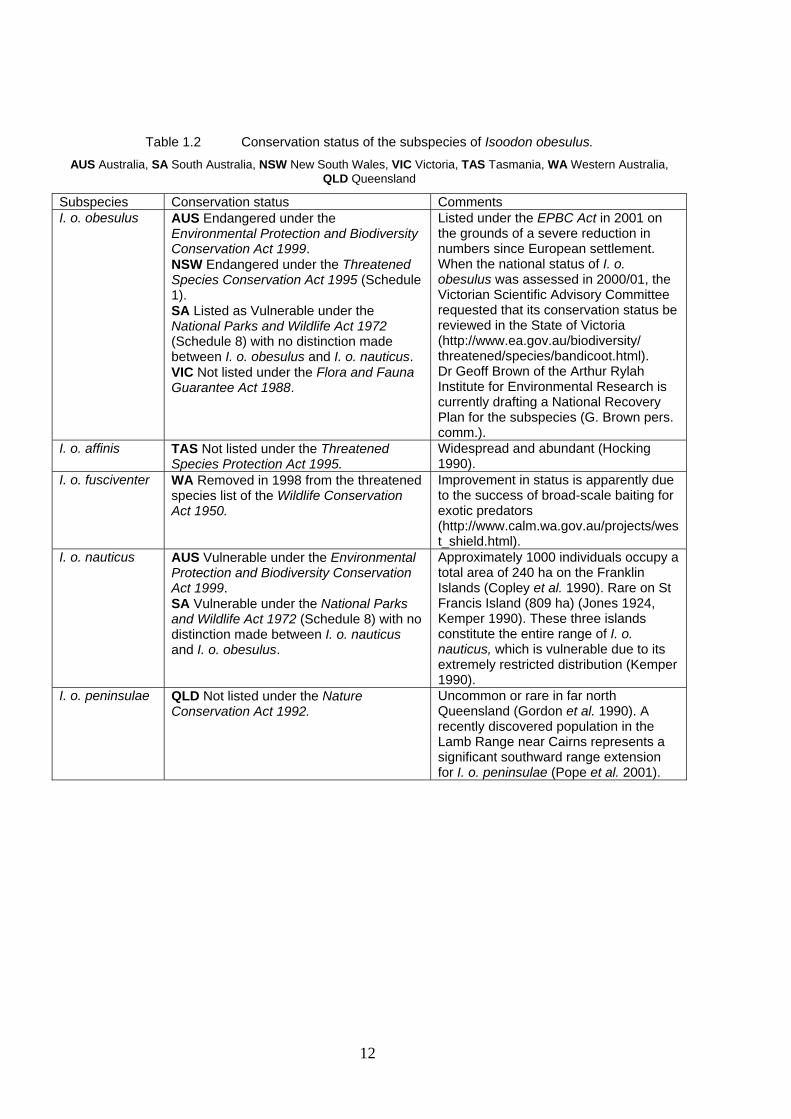
Table 1.2 Conservation status of the subspecies of Isoodon obesulus.

AUS Australia, SA South Australia, NSW New South Wales, VIC Victoria, TAS Tasmania, WA Western Australia, QLD Queensland

Subspecies Conservation status Comments I. o. obesulus AUS Endangered under the

Environmental Protection and Biodiversity Conservation Act 1999. NSW Endangered under the Threatened Species Conservation Act 1995 (Schedule 1). SA Listed as Vulnerable under the National Parks and Wildlife Act 1972 (Schedule 8) with no distinction made between I. o. obesulus and I. o. nauticus. VIC Not listed under the Flora and Fauna Guarantee Act 1988.

Listed under the EPBC Act in 2001 on the grounds of a severe reduction in numbers since European settlement. When the national status of I. o. obesulus was assessed in 2000/01, the Victorian Scientific Advisory Committee requested that its conservation status be reviewed in the State of Victoria (http://www.ea.gov.au/biodiversity/ threatened/species/bandicoot.html). Dr Geoff Brown of the Arthur Rylah Institute for Environmental Research is currently drafting a National Recovery Plan for the subspecies (G. Brown pers. comm.).

I. o. affinis TAS Not listed under the Threatened Species Protection Act 1995.

Widespread and abundant (Hocking 1990).

I. o. fusciventer WA Removed in 1998 from the threatened species list of the Wildlife Conservation Act 1950.

Improvement in status is apparently due to the success of broad-scale baiting for exotic predators (http://www.calm.wa.gov.au/projects/west_shield.html).

I. o. nauticus AUS Vulnerable under the Environmental Protection and Biodiversity Conservation Act 1999. SA Vulnerable under the National Parks and Wildlife Act 1972 (Schedule 8) with no distinction made between I. o. nauticus and I. o. obesulus.

Approximately 1000 individuals occupy a total area of 240 ha on the Franklin Islands (Copley et al. 1990). Rare on St Francis Island (809 ha) (Jones 1924, Kemper 1990). These three islands constitute the entire range of I. o. nauticus, which is vulnerable due to its extremely restricted distribution (Kemper 1990).

I. o. peninsulae QLD Not listed under the Nature Conservation Act 1992.

Uncommon or rare in far north Queensland (Gordon et al. 1990). A recently discovered population in the Lamb Range near Cairns represents a significant southward range extension for I. o. peninsulae (Pope et al. 2001).

http://www.ea.gov.au/biodiversity/threatened/species/bandicoot.html


http://www.calm.wa.gov.au/projects/west_shield.html


13

1.4 Sections of the Thesis

While differences in the conservation status of the southern brown bandicoot exist

between States, there is no doubt that the range of the species has contracted in the

last 200 years or so. There is also no doubt that the distribution has become more

fragmented at the three spatial scales examined in this thesis: continental, regional

and local. At each scale, the thesis seeks to identify the natural and human-induced

processes that have fragmented the distribution of the species. Commencing in

Chapter 2 at the continental scale, historical occurrence records and Geographic

Information Systems (GIS) analyses are used to model the spatial distribution of I. o.

obesulus in south-eastern Australia by combining climatic predictions with digital

maps of geology and vegetation in 1788 and 1988. By doing so a comparison is

made between habitat at the time of European settlement and two centuries later, thus

allowing factors that have caused fragmentation to be identified. The regional

distribution of I. obesulus in south-eastern South Australia is examined in Chapter 3

where predictions of habitat suitability are made by combining in a GIS a bioclimatic

model with digital maps of soil and vegetation at the time of European settlement

and at present. The local scale is examined in Chapters 4 and 5. In Chapter 4, surveys

for I. obesulus in 29 remnant patches of native vegetation in south-eastern South

Australia are described. The methods used to stratify remnants into sampling units

are explained and a field survey protocol outlined. Results of site surveys for the

presence/absence and abundance of I. obesulus are presented and statistical analyses

of the habitat variables that influence the local scale distribution of the species are

described. In Chapter 5, local scale habitat models are constructed using GIS to make

spatial and temporal predictions of habitat suitability under two fire management

scenarios. To conclude the thesis Chapter 6 summarizes the major findings of the

research, identifies key issues for the conservation of I. obesulus and highlights

future research directions.

15

CHAPTER 2 CONTINENTAL SCALE DISTRIBUTION OF ISOODON OBESULUS

2.1 Modelling the Distribution of Species

In this chapter the fragmented distribution of Isoodon obesulus is investigated at a

continental scale by combining bioclimatic modelling with habitat suitability

mapping techniques using Geographic Information Systems (GIS). Different

approaches are available for modelling the distribution of fauna; for example, habitat

suitability models, homocline matching models and probability approaches can be

used (Mackey and Lindenmayer 2001). The approach used in this chapter was to

create habitat suitability maps by overlaying weighted digital themes of climate,

geology and vegetation. The method for combining data was determined by

reviewing the species’ habitat requirements from published literature, through

investigating archived occurrence records and based on best professional judgement,

as described by Brooks (1997). Variables in habitat suitability index (HSI) models

are combined using simple equations and the strength of the approach lies in its

ability to make rapid and cost-effective assessments of wildlife habitat (Brooks

1997). It also offers a useful method for synthesising published habitat relations

(Mackey and Lindenmayer 2001). Bender et al. (1996) pointed out that a limitation

of the approach is that different habitat suitability indices may not represent real

differences between sites. Furthermore, the models are rarely tested with independent

distribution and abundance data (Brooks 1997, Mackey and Lindenmayer 2001). Due

to the lack of calibration in most HSI models, the values in the output usually lack

numerical meaning, other than being ordinal or ranked scores of suitability. If

reference areas of known population size are available, the values can be related to

the abundance of individuals or probability of their occurrence by use of resource

selection functions (Boyce and McDonald 1999). Nevertheless, the use of HSI

models is widespread and offers a powerful tool for assessing the quality of wildlife

habitat (Brooks 1997).

When analysing the distribution of cryptic species such as I. obesulus, a

common problem is posed by the paucity of basic distribution data. Typically such

16

data take the form of archived locality records. Many species are difficult to survey

in the field due to their small sizes, low population densities, secretive behaviours

and inaccessible habitats, so the collection of distribution data throughout a species’

entire geographic range is normally not feasible (Ponder et al. 2001). To get around

the problem of limited occurrence data, computer-modelling procedures using GIS

have been designed to predict the spatial distribution of species. Homocline

matching techniques using software such as BIOCLIM have been widely applied

(Brereton et al. 1995, Fisher et al. 2001, Lindenmayer et al. 1991, Olsen and Doran

2002). In these analyses, climatic profiles are generated of locations where the

species has been found and they are used to model its potential bioclimatic

distribution.

Based on fauna occurrence records and digital maps of environmental

resources, GIS spatial predictions can be made and used to direct field studies

towards areas where species are most likely to occur, thus optimizing limited

conservation resources (Ferrier 1991). Many occurrence records, however, have poor

spatial accuracy and can not be related directly to fine-grained spatial phenomena.

They may, therefore, be suitable for broad scale studies but their use is limited for

fine scale analyses.

2.2 Methods

In order to study the factors that influence the continental scale distribution of the

subspecies I. o. obesulus, habitat suitability models were created by combining

bioclimatic predictions of the subspecies’ distribution with maps depicting the

suitability of different geologic and vegetation classes. Occurrence records for I. o.

obesulus and literature references to its habitat were compiled and used to guide the

modelling of climatic, geologic and vegetation suitability for the subspecies. The

climate, geology and vegetation data were then overlaid with equal weightings to

produce continental scale predictions of habitat suitability for I. o. obesulus in 1788

and 1988.

17

2.2.1 Bioclimatic Modelling

A spatial prediction of climatic suitability for I. o. obesulus in south-eastern

Australia was made using ANUCLIM 5.1 (Houlder et al. 2000). BIOCLIM and

BIOMAP are two components of ANUCLIM and they were used to generate a

bioclimatic profile for I. o. obesulus and predict areas of Australia with suitable

climate for its occurrence.

The principal steps in the climatic prediction were:

a. acquiring and collating historical occurrence records of I. o. obesulus;

b. mapping the records, determining their elevation and assessing their accuracy;

c. screening the records for accuracy and reliability;

d. importing accurate and reliable records into BIOCLIM and calculating a

bioclimatic profile for I. o. obesulus;

e. identifying and removing outlying data points, then repeating BIOCLIM runs;

and

f. generating a BIOMAP prediction of areas where climate is suitable for the

subspecies.

Details of these six steps follow.

a. Acquisition and collation of occurrence records

Occurrence records for I. o. obesulus were obtained from the specimen collections of

the South Australian Museum, Museum Victoria and the Australian Museum. These

records gave the location where each specimen was found (in latitude and longitude)

and other information including acquisition dates and collectors’ identities.

Additional records were obtained from the Atlas of Victorian Wildlife computer

database and the New South Wales Parks and Wildlife Service computer database of

species locality records. Trapping data, field observations and anecdotal accounts of

I. o. obesulus gathered from reliable witnesses in South Australia and south-western

Victoria were compiled by the author and Michael Rees (Paull 1993, 1995, Rees

1997, Rees and Paull 2000) and combined with the sources listed above.

Information from these records was compiled in a spreadsheet containing

fields for geographic coordinates, year of collection or observation, type of record

(e.g. museum specimen or observed) and reliability of identification of the

18

subspecies (Appendix A1). Duplication of records existed between some of the data

sources; for example, Museum Victoria records were also listed in the Atlas of

Victorian Wildlife. In these cases only the original records were entered. When

combined in this manner, there was a total of 1561 locality records of I. o. obesulus

although, as explained below in Section 2.2.1c, not all were valid or reliable.

b. Mapping the records

The records were plotted onto 1:100 000 or 1:50 000 topographic maps depending on

availability. Careful judgement was exercised when interpreting the records because

a variety of coordinate systems was used, including degrees-minutes-seconds,

decimal degrees and Australian Map Grid references. In some cases locality

descriptions such as ‘3.2 km SW of Glencoe’ were available. Once plotted,

Australian Map Grid coordinates (Easting and Northing, AGD66) were read for each

record and an assessment was made of the probable horizontal (XY) error based on

the original description. To determine elevation, the nearest contour value was noted

and an estimate was made of the vertical (Z) error based on variation in contour

values within the zone defined by the XY error. The mapped records and their ages

are shown in Figure 2.1.

c. Record screening

Before being entered into BIOCLIM, records were screened for type, reliability of

identification and spatial accuracy. Not all types of records were suitable for

BIOCLIM analysis. For example, records of I. o. obesulus hairs found in predator

scats were omitted because scats are located an unknown distance from where

predators consume their prey. Subfossil records, usually from cave deposits, were

also excluded from analysis because their age was unknown and climatic conditions

may have changed since the death of the specimens. Indirect observations of I. o.

obesulus, including nests and the conical foraging pits that it makes in topsoil, were

also excluded from analysis. Records from Eyre Peninsula in South Australia and

from north of the Hawkesbury River in New South Wales were rejected because it is

doubtful that they refer to I. o. obesulus (Dixon 1978, Joan Dixon pers. comm., Paull

1995, Cath Kemper pers. comm., Peter Johnston pers. comm.).

19

#

#

#######Ñ###

Ñ

##########

Ñ

#

##

#

#

#

#

Ñ

### ###

#

ÑÑÑÑÑ

#

#

Ñ

#

Ñ

SSSSS

#

#

##

##

#

#

#

##

#

#

#

#

#

#

#

##

#

#

#

#########

# ##

#

#####

##

#

#

###

#####

##

##

##

##

#

##

#

#

#

#

##

#

#

###

##

## #######

##

#

### #

#

#

#

#

# ####

## #### ###

## ### ## ##

# ###ÑÑÑ###########Ñ#

##### #Ñ ###

#

Ñ

#

#

####

##

#

#

##

#

###

#

##S #

##S#####

#

# ##############

###############

#

#

#

#####

#

#

#

#

#

##

##

## #

#

#

###

###ÑÑÑÑ

############

####

#

## #

###

####

#

Ñ###

####ÑÑÑÑÑÑÑÑÑÑÑÑÑ###

##### #

#Ñ## ###

######

###

##

Ñ#

#

#

### ###Ñ ####

##

#

#

#

##

#

#

######

##

###

##

##

#

##

###

###### ##

####

####

##

# #

##

#

#

#####

##### ##

####

##

###

#

#

##

S

#

##

#

#

##

#

#

##

Ñ ÑÑ

#

##

##

#

################

SSSS

#

#

###

###### #

##

#

#

###

#

#

##

###

###

Ñ

Ñ###

#

ÑÑ

#Ñ#

#

#

#

#

#

# ##

#

##

#

##

#

#

#

#

# #### S

##

#

##

#

#

Ñ#

#

#

###

#

##

Ñ

#

#

# #

########

Ñ

#

##

#

#

### ####

#

##

#####

##

##

#

#

#

##

#

#####

#

#

#

###

#

#

#####

##

#

###

#

##

###S#S##

###

#

#

##

#

#

Ñ

##

##

Ñ

#

S

#

####

Ñ##Ñ

###Ñ ######

######

#Ñ###Ñ### ## ##########

######### # ####

#

#### #

###

#

Ñ##

#

##

#

###########

#

######S##

#

#

#####

#

###

##

#

#

#

#

###

#

##########

##

ÑÑÑÑÑÑÑÑÑ

###

#####

####

#####

#

#

#####################

# ÑÑ#

#Ñ

##

##

##

#

##

###

#

###

#

##

#

# ### ####

##

#####

#

#

##

##

######

#

##

#

#

#

###

##

########

##

#

#

#

#

####

##

########

#

######

##

#

S

#

#

#

#

# #

ÑÑ#

##ÑÑ

ÑÑ ÑÑÑ

ÑÑÑÑÑ

ÑÑÑÑ

ÑÑ

ÑÑÑÑÑÑÑ

ÑÑ#########################################################

########### ########## ###

##

#

#

# #########

##

## ###

###

#Ñ#

Ñ

##

#

#

ÑÑÑÑÑÑÑÑÑÑÑÑÑÑÑÑÑÑÑÑÑÑÑÑÑÑÑ######ÑÑÑÑ##

##

#

#

####

#

###

Ñ

##

###

##

#

#

S

##

####

#

#

## #######

### #

##

##

#

Ñ

Ñ

ÑÑÑÑÑÑÑÑÑÑÑÑÑÑÑÑÑÑÑÑÑÑÑÑÑÑÑÑÑÑÑÑÑÑÑÑÑÑÑÑÑÑÑÑÑÑ

ÑÑÑÑÑÑÑÑÑÑÑÑÑÑÑÑÑÑÑÑÑÑÑÑÑÑÑÑÑÑÑÑÑÑÑÑÑÑÑÑÑÑÑÑÑÑÑÑÑ ÑÑÑÑÑÑÑÑÑÑÑÑÑÑÑÑÑÑÑÑÑÑÑÑÑÑÑÑÑÑÑÑÑÑÑÑÑÑÑÑÑÑ

ÑÑ

##

S

S

S

S

S

S#

###

#

##

### ##

###

#

#

#

#

#

# #

##

#

Ñ

##

#

##S

##

#

# ##

#

##

#

#

###################

## #

#

#

#

#

###

## #####

#

############# ######

#######

########

### ############# #

###

#####

###### #

Ñ#

#

##

###

#

## #

###

#### #

###

###

###

# ##

##

###

# ###

#

##

#

##

S

##

####

##

#

N

0 200 km

subfossil/unknownS

pre 1951#

1951 - 1975#

1976 - 1985#

1986 - 1995#

post 1995Ñ Figure 2.1 Occurrence records attributed to Isoodon obesulus obesulus.

Not all 1561 records are valid or reliable.

# ##########

###########

####

###################

##

#

#

##

#

##

# ###### #########

############# ########

#

####

##

#

#

#

#

#

########

#

#

##

#

#

#

# #

#

#

#

### #

#

##

#

#

#

##

##

# ####

####### ##

###

#######

### ######## #

#

#

# #

#

##

#

###

##

#

#### ##

#

#

###

#

######

##

##

#

##

#

#

#

#

#

#####

##

##

#

#

#

#########

####

#

#

##

##

#

#

#

#

#

#

#

##

#

#

##

##

##

#

##

#

##

#

#

##

#

##

#

#

##

#

#

#

##

#

#

#

#

##

#

##

#

###

##

#

## ##

#

#

##

##

######

###

#

#

#

##

#

#

#

#

#

#

##

#

#

#

##

#

#

#

#

######

#

#

#

#

#

##

#

##

#

#

##

#

##

#

#

#

#

#

#

#

# #

##

#

#

#

#

#

#

#

#

#

#

#

#

#

#

##

# #

##

#

#

##

#

#

#

#

#

#

#

#

#

#

##

#

##

#

##

#

#

#

##

#

#

###

#

#

###

#

##

#

# ##

##

####

## ##

#####

#

# ###

#

#

##

#

#

#

###

######

#

##########

##

#

##

#

###

#

######################

## ## ####

#

##

#

#

#

###

#

##

#

#

#########

#

##

#

#

#

# #

#

##

#

#

#

#

N

0 200 km

BIOCLIM outliers#

modelling records#

validation records#

KI

GRA

MLR

MGP

OTG MWP

EGE

BBD

SYD

Figure 2.2 Records used to model and validate the distribution of Isoodon obesulus obesulus at the continental scale.

Black dots represent 323 records used to make the BIOMAP predictions and develop the weighting system for geologic and vegetation suitability maps. Green dots represent 229 records used to test the validity of climate, geologic and vegetation suitability predictions. Red dots indicate 15 outlying records that were removed prior to

making the final BIOMAP predictions.

KI Kangaroo Island, MLR Mount Lofty Ranges, MGP Mount Gambier to Portland, GRA Grampian Ranges, OTG Otway Ranges to Geelong, MWP Melbourne to Wilsons Promontory, EGE East Gippsland to Eden, BBD Batemans

Bay to Durras, SYD Sydney.

20

Only the most accurate records, with an estimated XY error less than 1500 m

were selected for climatic modelling. Furthermore, BIOCLIM analyses require

accurate elevation data (Houlder et al. 2000). Only those records with an estimated Z

error <40 m were, therefore, used. Finally, in situations where two or more records

had the same geographic coordinates, only the most recent record was chosen. At the

conclusion of the screening process, 338 records dated between 1895 and 2000 were

available for use as an initial modelling set (Figure 2.2).

d. Record input and generation of bioclimatic profiles

A tab delimited, text format file containing 338 modelling records was imported into

BIOCLIM. This file contained four fields, being record reference number, X

coordinate (longitude in decimal degrees), Y coordinate (latitude in decimal degrees)

and elevation (in metres). In BIOCLIM, the format of the fields was defined and a

climatic profile of the data and a site report were computed. The profile file (*.pro)

provided summary statistics for the input data, including maximum, minimum, mean,

standard deviation and percentile distributions for 35 bioclimatic parameters

(Appendix A2). This file was required for the final stage of bioclimatic modelling

when BIOMAP spatial predictions were made. The calculation of bioclimatic

parameter values was based on five default climatic surfaces contained within

ANUCLIM, being maximum temperature (oC), minimum temperature (oC), rainfall

(mm), radiation with rainfall (MJ/m2/day) and evaporation (mm/month). BIOCLIM

was used to calculate parameter values for each record in the input data and the

results were saved in a *.bio file. These values were used to identify outlying data.

e. Identifying outlying data and repeating BIOCLIM runs

An important stage in the BIOCLIM process is the analysis of outlying data because

extreme points have the potential to adversely influence BIOMAP predictions

(Houlder et al. 2000). BIOCLIM produces cumulative frequency plots of the input

data for each of the climatic parameters. When these 35 graphs were inspected for

extreme values, 15 records out of the 338 contained in the initial modelling dataset

consistently appeared to be outliers. These points were removed, reducing the input

dataset to 323 records (Figure 2.2). BIOCLIM parameter values were recalculated

for the reduced dataset and outlying records were no longer apparent.

21

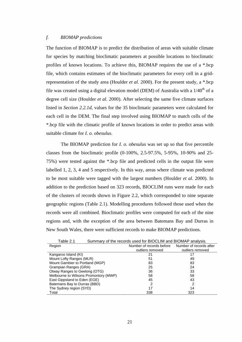
f. BIOMAP predictions

The function of BIOMAP is to predict the distribution of areas with suitable climate

for species by matching bioclimatic parameters at possible locations to bioclimatic

profiles of known locations. To achieve this, BIOMAP requires the use of a *.bcp

file, which contains estimates of the bioclimatic parameters for every cell in a grid-

representation of the study area (Houlder et al. 2000). For the present study, a *.bcp

file was created using a digital elevation model (DEM) of Australia with a 1/40th of a

degree cell size (Houlder et al. 2000). After selecting the same five climate surfaces

listed in Section 2.2.1d, values for the 35 bioclimatic parameters were calculated for

each cell in the DEM. The final step involved using BIOMAP to match cells of the

*.bcp file with the climatic profile of known locations in order to predict areas with

suitable climate for I. o. obesulus.

The BIOMAP prediction for I. o. obesulus was set up so that five percentile

classes from the bioclimatic profile (0-100%, 2.5-97.5%, 5-95%, 10-90% and 25-

75%) were tested against the *.bcp file and predicted cells in the output file were

labelled 1, 2, 3, 4 and 5 respectively. In this way, areas where climate was predicted

to be most suitable were tagged with the largest numbers (Houlder et al. 2000). In

addition to the prediction based on 323 records, BIOCLIM runs were made for each

of the clusters of records shown in Figure 2.2, which corresponded to nine separate

geographic regions (Table 2.1). Modelling procedures followed those used when the

records were all combined. Bioclimatic profiles were computed for each of the nine

regions and, with the exception of the area between Batemans Bay and Durras in

New South Wales, there were sufficient records to make BIOMAP predictions.

Table 2.1 Summary of the records used for BIOCLIM and BIOMAP analysis. Region Number of records before

outliers removed Number of records after

outliers removed Kangaroo Island (KI) 21 17 Mount Lofty Ranges (MLR) 51 49 Mount Gambier to Portland (MGP) 83 83 Grampian Ranges (GRA) 25 24 Otway Ranges to Geelong (OTG) 36 33 Melbourne to Wilsons Promontory (MWP) 58 58 East Gippsland to Eden (EGE) 45 43 Batemans Bay to Durras (BBD) 2 2 The Sydney region (SYD) 17 14 Total 338 323

22

2.2.2 Climate Suitability Mapping

To create a climate suitability map for I. o. obesulus, BIOMAP predictions were

imported into ArcView 3.2a where they were converted from shapefiles into grid

files with a cell size of 0.025 degrees and an extent the same as that shown in Figure

2.2. The BIOMAP output values were treated as suitability indices, or weights,

ranging from 0 (not predicted by BIOMAP) to 5 (predicted from the 25-75%

percentile class of the bioclimatic profile). The climate suitability map was

constructed by first merging the grids of the eight separate geographic regions

modelled with BIOMAP into one raster and secondly using ArcView’s Map

Calculator to add the values from the merged grid to the BIOMAP prediction using

323 combined records. To the resulting grids, 1 was added to remove zero values

from the output and to make the maximum value 10.

2.2.3 Geologic Suitability Mapping

The National Digital Geoscience Datasets Version 1.1 (Kilgour and Wyborn 1998)

were obtained from Geoscience Australia and used with ArcView to develop a

geologic suitability map for I. o. obesulus. From these datasets Lithological

Association and Regolith Class with a nominal scale of 1:5 000 000 were chosen for

analysis (Figure 2.3) because they were most relevant to the subspecies’ continental

scale distribution when compared to other themes such as Aquifer Type and

Metamorphic Type. Little is known about the relationship between the distribution of

I. o. obesulus and geologic substrates, although the subspecies has been associated

with sandy soils having well-drained upper horizons (Emison et al. 1975, Menkhorst

and Seebeck 1990, Opie et al. 1990). Its absence has also been correlated with some

lithologies, for example volcanic plains in western Victoria (Menkhorst 1995).

Suitability weights in the range of 1-5 were assigned to the Lithological

Association and Regolith Class maps based on the number of records and relative

area of each attribute class. Lithological Association and Regolith Class were

rasterised to the same extent and cell size as the climate suitability map and

reclassified using the assigned suitability weights. The values in the reclassified grids

of Lithological Association and Regolith Class were then added together using

ArcView’s Map Calculator to produce a geologic suitability map for I. o. obesulus.

23

N

0 200 km

alkaline igneous rocks

felsic to mafic volcanics

felsic volcanics

granites

granulite-facies metamorphics

intrusive complexes

mafic volcanics

mafic-ultramafic intrusives

sedimentary rocks

serpentinites

volcaniclastic sedimentary rocks

N

0 200 km

aeolian sand

alluvial sediments

beach sediments

evaporite

highly weathered bedrock

moderately weathered bedrock

residual clay

residual material

residual sand

slightly weathered bedrock

soil on bedrock

terrestrial sediments

very highly weathered bedrock

a

b

Figure 2.3 a Lithological Association and b Regolith Class of the study area.

24

2.2.4 Vegetation Suitability Mapping

Vegetation suitability maps were created using a similar method to the geologic

suitability map. Digitised versions of the Vegetation of Australia 1788 and

Vegetation of Australia 1988 were obtained from Geoscience Australia and four

themes were chosen to analyse change in vegetation over 200 years since the time of

European settlement. The vegetation themes were:

a. dominant species of the tallest stratum,

b. growth form of the tallest stratum,

c. density of the tallest stratum, and

d. growth form of the lowest stratum (Figure 2.4).

These themes were selected because they each covered the study area at a nominal

scale of 1:5 000 000 and they were relevant to the structure and composition of

vegetation found in I. o. obesulus habitats.

The 323 modelling records were compared against the four vegetation themes

from the 1788 and 1988 maps and suitability weights were assigned as before but

this time the value 0 was included. When the value zero was combined with other

data in the habitat suitability maps, it was not treated as a zone of exclusion, which a

binary response (0,1) would require; instead when layers were combined using

addition, 0 in the input maps made no contribution to the output. Previous

observations of habitat use by I. o. obesulus influenced the weighting of vegetation

(Table 2.2), which was not possible for geologic suitability mapping. Allocation of

suitability weights to vegetation classes was guided not only by the number of

records falling into the classes but also by past observations of the species’ habitat

use.

These weights were used to create suitability maps for I. o. obesulus for each

of the vegetation attributes in 1788 and 1988. In the same way that the geologic

suitability map was produced, the four vegetation layers for each date were added

together using ArcView’s Map Calculator then reclassified by ten equal interval

classes to produce vegetation suitability maps for 1788 and 1988.

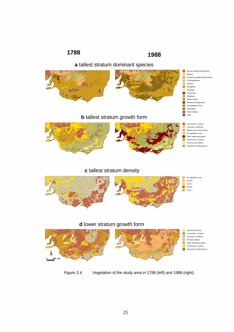
25

1788 1988a tallest stratum dominant species

N

0 250 km

Acacia including Racosperma

Banksia

Casuarina including Allocasuarina

Chenopodiaceae

Conifers

Eucalyptus

Fabaceae

Graminoids

Melaleuca

Mixed or other

Myoporum (sugarwood)

No vegetation cover

Nothofagus

Other Grasses

Stipa

N

0 250 km

N

250 km

Hummock Grasses

Low shrubs <2 metres

Low trees <10 metres

No lower stratum

Other herbaceous plants

Tall Shrubs >2 metres

Tussocky or tufted grasses

0 200 km

N

250 km

N

0 250 km

Low shrubs <2 metres

Low trees <10 metres

Medium trees 10-30 metres

No vegetation cover

Other herbaceous plants

Tall Shrubs >2 metres

Tall trees >30 metres

Tussocky or tufted grasses

b tallest stratum growth form

N

250 km

N

0 250 km

No vegetation cover

lO-3O%

<1O%

30-70%

>70%

c tallest stratum density

d lower stratum growth form

Figure 2.4 Vegetation of the study area in 1788 (left) and 1988 (right).

26

2.2.5 Habitat Suitability Mapping

Continental scale predictions of habitat suitability for I. o. obesulus were made by

combining climate, geologic and vegetation suitability maps. By adding the 1788 and

1988 vegetation suitability maps in turn to the climate suitability and geologic

suitability maps, two map calculations were performed to predict habitat suitability.

The two map calculations were reclassified to a 10-class habitat suitability index

using the scheme shown in Table 2.3 instead of equal intervals used for the

vegetation suitability maps in order to avoid emphasizing low values. Based on the

assumption that the distribution of areas with suitable climate and geology have not

altered since 1788, these maps predicted change to the distribution of I. o. obesulus

as a result of vegetation change.

Table 2.2 Types of vegetation used by Isoodon obesulus obesulus.

Region Vegetation types

Kangaroo Island Eucalyptus woodlands, coastal shrublands, heathlands and mallee (Paull 1993).

Mount Lofty Ranges Eucalyptus obliqua open forests and woodlands with heath-associated plants in the shrub and ground layers (Paull 1993).

South-eastern South Australia

Low and medium Eucalyptus baxteri woodlands with sparse shrub and dense heath ground layers (Paull 1993).

South-western Victoria Open and low-open forests of Eucalyptus baxteri and Eucalyptus obliqua, open and closed Banksia marginata heathlands, Melaleuca squarrosa closed scrubs, coastal shrublands and coastal heathlands (Menkhorst and Beardsell 1982, Rees 1997).

Grampians Heathlands (Lobert and Lee 1990).

Otway Ranges Eucalyptus baxteri open forests and habitats dominated by Allocasuarina paludosa and Leptospermum continentale (Moro 1991, Wilson et al. 1990).

Melbourne region Heathlands and shublands dominated by Leptospermum myrsinoides, Melaleuca squarrosa, Banksia marginata, Gahnia sieberiana and Leptospermum continentale (Braithwaite 1983, Braithwaite and Gullan 1978, Lobert 1985, Lobert and Opie 1986, Opie 1980, Stoddart and Braithwaite 1979).

East Gippsland Leptospermum myrsinoides heathlands, Banksia woodlands, coastal heathlands, damp sclerophyll forests and coastal sclerophyll forests (Opie et al. 1990).

South-eastern New South Wales

Associations dominated by Eucalyptus sieberi, Eucalyptus agglomerata, Eucalyptus globoidea, Eucalyptus cypellocarpa and Eucalyptus gummifera (Andrew Claridge pers. comm.).

Sydney region Open Eucalyptus woodlands and heathlands on sandstone ridges. Associations of Eucalyptus sieberi, E. capitellata, E. gummifera, E. sparsifolia, E. racemosa, E. piperita, E. pilularis, Angophora costata (Andrew Claridge pers. comm.).

27

2.2.6 Model Validation

To assess the performance of the spatial predictions, a set of validation records,

independent from the modelling records, was compared against the indices in the

suitability maps. The same criteria described in Section 2.2.1c for type of record and

reliability of identification were used to select the validation records. It was not

necessary to consider the potential elevation error and XY errors up to 2500 metres

or approximately one grid cell in the GIS rasters were tolerated. To ensure that only

one record fell within any particular cell of the output maps, validation records were

chosen that were at least 2500 m from their nearest neighbour. By applying these

criteria, a selection of 229 records dating from 1969 was made for validating the

habitat suitability maps.

Table 2.3 Reclassification scheme for the habitat suitability index.

Sum of Climate Suitability + Geologic Suitability + Vegetation Suitability

Habitat Suitability Index

1-12 1 13-14 2 15-16 3 17-18 4 19-20 5 21-22 6 23-24 7 25-26 8 27-28 9 29-30 10

28

2.3 Results

2.3.1 Climate Suitability

The BIOMAP model based on 323 points is shown in Figure 2.5a. Two areas, extra-

limital to the known distribution of I. o. obesulus, were predicted in north-eastern

Tasmania (199 cells or approximately 119 400 ha) and near Albany in Western

Australia (682 cells or approximately 409 200 ha). The BIOMAP values for these

extra-limital areas, which slightly overlapped the known distributions of I. o.

fusciventer and I. o. affinis, were in the range of 1-2. The model predicted major

climatic disjunctions within the distribution of I. o. obesulus at the Coorong

(between the Mount Lofty Ranges and the Mount Gambier to Portland regions), Port

Phillip Bay (between the Otway Ranges to Geelong and Melbourne to Wilsons

Promontory regions) and the La Trobe Valley (between Melbourne to Wilsons

Promontory and East Gippsland to Eden regions), which closely matched the known

distribution of the subspecies (Figure 1.3). Climatic disjunctions were also apparent

at the Illawarra region (between the Batemans Bay to Durras and Sydney regions).

Investigator Strait (between Kangaroo Island and the Mount Lofty Ranges) was not

included on the DEM from which the *.bcp file was calculated and, therefore, it was

not predicted by BIOMAP.

The areas with the most suitable climate were predicted to be in south-eastern

South Australia and south-western Victoria, followed by the area from Melbourne to

Wilsons Promontory, the Mount Lofty Ranges and East Gippsland. The predictions

for New South Wales and Kangaroo Island, at the eastern and western extremities of

the subspecies’ distribution, were of relatively low climatic suitability (BIOMAP

values <3) compared to other regions and this was probably influenced by the small

number of accurate and reliable records available from there. In the Sydney region,

38 cells or approximately 22 800 ha were modelled to have a BIOMAP value of 1.

Suitable climate was not predicted for Eyre Peninsula in South Australia, Maldon in

central Victoria, north of the Hawkesbury River, the Blue Mountains and Kahncoban

in New South Wales, all of which are associated with unconfirmed records of I. o.

obesulus (Figure 2.1).

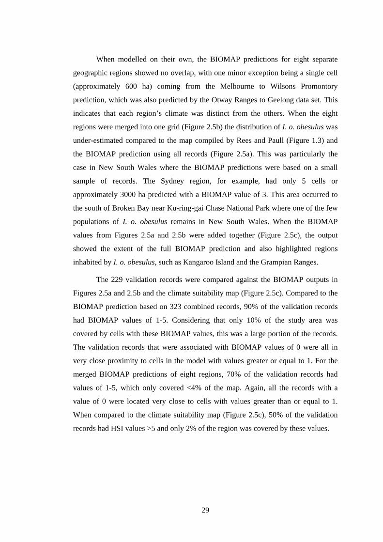
29

When modelled on their own, the BIOMAP predictions for eight separate

geographic regions showed no overlap, with one minor exception being a single cell

(approximately 600 ha) coming from the Melbourne to Wilsons Promontory

prediction, which was also predicted by the Otway Ranges to Geelong data set. This

indicates that each region’s climate was distinct from the others. When the eight

regions were merged into one grid (Figure 2.5b) the distribution of I. o. obesulus was

under-estimated compared to the map compiled by Rees and Paull (Figure 1.3) and

the BIOMAP prediction using all records (Figure 2.5a). This was particularly the

case in New South Wales where the BIOMAP predictions were based on a small

sample of records. The Sydney region, for example, had only 5 cells or

approximately 3000 ha predicted with a BIOMAP value of 3. This area occurred to

the south of Broken Bay near Ku-ring-gai Chase National Park where one of the few

populations of I. o. obesulus remains in New South Wales. When the BIOMAP

values from Figures 2.5a and 2.5b were added together (Figure 2.5c), the output

showed the extent of the full BIOMAP prediction and also highlighted regions

inhabited by I. o. obesulus, such as Kangaroo Island and the Grampian Ranges.

The 229 validation records were compared against the BIOMAP outputs in

Figures 2.5a and 2.5b and the climate suitability map (Figure 2.5c). Compared to the

BIOMAP prediction based on 323 combined records, 90% of the validation records

had BIOMAP values of 1-5. Considering that only 10% of the study area was

covered by cells with these BIOMAP values, this was a large portion of the records.

The validation records that were associated with BIOMAP values of 0 were all in

very close proximity to cells in the model with values greater or equal to 1. For the

merged BIOMAP predictions of eight regions, 70% of the validation records had

values of 1-5, which only covered <4% of the map. Again, all the records with a

value of 0 were located very close to cells with values greater than or equal to 1.

When compared to the climate suitability map (Figure 2.5c), 50% of the validation

records had HSI values >5 and only 2% of the region was covered by these values.

30

Figure 2.5 BIOMAP outputs and the climate suitability map.

a BIOMAP output for 323 records, b BIOMAP outputs merged from eight separate geographic regions, and c climate suitability map created by adding the values of Figures 2.5a and 2.5b, plus 1.

31

2.3.2 Geologic Suitability

The highest suitability weight (5) for Lithological Association was assigned to

sedimentary rocks because 279 (86%) of the modelling records corresponded to this

class, which was roughly in proportion to its area (Table 2.4). Granites were ranked

next highest in suitability, with records in this class occurring in East Gippsland to

Eden, Melbourne to Wilsons Promontory, the Grampian Ranges and on Kangaroo

Island. Menkhorst (1995) observed that I. o. obesulus was absent on the volcanic

plains of western Victoria but 12 records came from areas of mafic volcanics in the

vicinity of Portland and Geelong, which are on the margins of the volcanic plain.

Other classes of Lithological Association with one record each were felsic volcanics,

granulite-facies metamorphics and felsic to mafic volcanics and they were given a

weight of 2. The remaining five classes were not associated with any records of I. o.

obesulus and they were given a weight of 1. For Regolith Class, the highest weight

Table 2.4 Geologic suitability weights. Weights were based on the frequency of records and area of each geologic class.

Geologic attribute Records (N) Area (%) %R/%A Weight LITHOLOGICAL ASSOCIATION sedimentary rocks 279 80.9 1.1 5 granites 29 8.3 1.1 4 mafic volcanics 12 5.3 0.7 3 felsic volcanics 1 3.7 0.1 2 granulite-facies metamorphics 1 0.9 0.3 2 felsic to mafic volcanics 1 0.3 1.0 2 volcaniclastic sedimentary rocks - 0.4 - 1 mafic-ultramafic intrusives - <0.1 - 1 serpentinites - <0.1 - 1 intrusive complexes - <0.1 - 1 alkaline igneous rocks - <0.1 - 1 REGOLITH CLASS beach sediments 79 2.4 10.1 5 highly weathered bedrock 56 20.2 0.9 4 moderately weathered bedrock 50 21.3 0.7 4 soil on bedrock 49 5.3 2.9 5 residual sand 49 1.8 8.4 5 residual clay 21 0.3 18.9 4 slightly weathered bedrock 10 2.1 1.5 3 aeolian sand 5 20.4 0.1 2 residual material 4 0.4 3.0 2 alluvial sediments - 14.9 - 1 terrestrial sediments - 10.3 - 1 very highly weathered bedrock - 0.3 - 1 evaporite - 0.2 - 1

32

(5) was allocated to beach sediments because this attribute had the highest number of

records associated with it. Soil on bedrock and residual sand were also given a

weight of 5 because the percentages of records in these two classes were high in

relation to the areas they covered. The next highest weighted classes (4) were highly

weathered bedrock and moderately weathered bedrock, which were associated with

56 and 50 records respectivley and residual clay with 21 records but covering only

0.3% of the study area in the Otway Ranges to Geelong region.

When the weights were applied to the Lithological Association map, large

areas with high suitability (>7) for I. o. obesulus were predicted (Figures 2.6a) and

this included all regions of the study area inhabited by the species. There was little

evidence that Lithological Association contributed to the fragmented continental

distribution of I. o. obesulus, with the exception of mafic volcanics in western

Victoria which fragment the Otway Ranges to Geelong region from all other regions.

When the weights were applied to Regolith Class (Figures 2.6b) three of the regions

inhabited by I. o. obesulus were highlighted, being the Mount Lofty Ranges, the

Mount Gambier to Portland region and the Melbourne to Wilsons Promontory

region. When both geologic themes were combined (Figure 2.6c), the prediction of

geologic suitability more closely resembled the known distribution of the subspecies

(Figure 1.3). A notable exception was the Sydney region, which was predicted as

having lower geologic suitability (7) for I. o. obesulus than areas immediately

surrounding it and the other regions being studied (Figure 2.6c). This was because of

the low weight (2) given to residual material in the reclassification of the Regolith

Class map. The prediction for Victoria and South Australia was of high values of

geologic suitability (>7) in regions where the subspecies is known to occur. The

geologic suitability map included many areas where the species has not been

recorded and that were not predicted using BIOCLIM and BIOMAP. It was therefore

less effective at explaining the fragmented continental scale distribution of I. o.

obesulus than the climatic prediction.

Compared to the weighted lithological suitability map (Figure 2.6a), the

percentage of validation records associated with each suitability weight was roughly

proportional to the area of the map covered by that weight (Appendix A3). This was

not surprising because 81% of the study area was mapped with a weight of 5. For the

33

regolith suitability map, a very high percentage of validation records coincided with

the higher weights and very few records with the lower weights. When compared to

the geologic suitability map, which combined lithology and regolith, none of the

validation records had suitability indices <5, although only 2% of the study area had

such low values. For the areas mapped with suitability indices 5-10, there was an

increasing probability of validation records coinciding with higher geologic

suitability indices.

Figure 2.6 Geologic suitability maps.

a lithological suitability, b regolith suitability, c geologic suitability, created by adding the weighted maps shown in Figures 2.6a and 2.6b.

34

2.3.3 Vegetation Suitability in 1788 and 1988

The frequency of records for each vegetation class and the suitability weights that

were assigned are shown in Table 2.5. Because the two vegetation datasets, 1788 and

1988, had different classifications, it was necessary to devise a weighting system that

could be applied to both. Additionally, because the I. o. obesulus records were not

contemporaneous with either theme, careful judgment was used when assigning

weights and was guided by Table 2.2.

For the attribute Tallest Stratum Dominant Species the highest weight (5) was

given to Eucalyptus because most records fell into this class in 1788 and 1988.

Where discrepancies existed between the 1788 and 1988 maps, they were attributed

to land cover change between the two dates, not a change in habitat selection by I. o.

obesulus. For example, no records fell into the class conifers in the 1788 map but 37

did so in the 1988 map. Similarly, only 2 records fell into the class other grasses in

the 1788 map but 105 did so when compared to the 1988 map. Neither conifers nor

other grasses were considered to be vegetation types commonly used by I. o.

obesulus but a weight of 2 was, nevertheless, assigned to each of these classes. The

small area of the class conifers compared to the number of records associated with it

was also taken into account when assigning this weight. The class no tallest stratum,

which applied to waterbodies and urban areas devoid of native vegetation, was

assigned a weight of 0.

The greatest weight (5) for Tallest Stratum Growth Form was assigned to

medium trees, which was the class associated with the greatest number of records in

both 1788 and 1988. The class low trees was given a weight of 4 based on a high

number of records in both 1788 and 1988. The class other herbaceous plants was not

included in the 1788 mapping but was represented by 105 records in the 1988 theme.

It was therefore given a weight of 2. The classes tall shrubs >2 m and low shrubs <2

m had no records associated with them but were given a weight of 2 based on

existing knowledge of habitat use by I. o. obesulus (Table 2.2).

For Tallest Stratum Density, areas with 30-70% cover had the greatest

number of records in both years and were therefore assigned a weight of 5. Sparser

and denser classes were assigned lower weights after considering the records and

35

relative areas. The highest weight (5) for Lower Stratum Growth Form was given to

low shrubs <2 m because this class contained the greatest number of records when

compared to the 1788 map. No lower stratum in the 1988 map contained the greatest

number of records but it was given a weight of 0. This was because the class no

lower stratum coincided with other grasses and graminoids in the Tallest Stratum

Dominant Species theme. The weights assigned to remaining classes were decided

upon after considering record frequencies and relative areas. Table 2.5 Vegetation suitability weights.

- no data, * not represented in the mapping Weights were assigned based on the record frequencies and extent of each vegetation class, as well

as literature references to habitat use by Isoodon obesulus. Compared to 1788 map Compared to 1988 map Vegetation attribute Records

(N) Area(%)

%R/%A

Records (N)

Area (%)

%R/ %A

Weight

TALLEST STRATUM DOMINANT SPECIES Eucalyptus 321 71.3 1.4 170 40.3 1.3 5 Other Grasses 2 1.9 0.3 105 37.8 0.9 2 Banksia - 0.4 - - 0.3 - 2 Casuarina including Allocasuarina - 6.2 - - 5.0 - 2 Conifers - 0.4 - 37 0.9 12.6 2 Mixed or other - 2.3 - 1 1.9 0.2 1 Chenopodiaceae (eg saltbush and bluebush) - 9.0 - - 7.8 - 1 Acacia including Racosperma - 4.8 - - 3.3 - 1 undescribed - 1.5 - * * - 1 Myoporum (sugarwood) - 1.2 - - 1.2 - 1 Melaleuca - 0.3 - - 0.1 - 1 Nothofagus - <0.1 - - <0.1 - 1 Graminoids - 0.2 - * * * 1 Fabaceae (includes clovers and medics) * * * - <0.1 - 1 No tallest stratum - 0.4 - 10 1.2 2.5 0 TALLEST STRATUM GROWTH FORM Medium trees 10-30 m 264 44.7 1.8 166 24.5 2.1 5 Low trees <10 m 46 21.0 0.7 35 15.0 0.7 4 Other herbaceous plants * * * 105 22.1 1.5 2 Tall trees >30 m 11 3.4 1.0 7 3.0 0.7 2 Tussocky or tufted grasses 2 3.7 0.2 - 15.8 - 2 Tall Shrubs >2 m - 17.2 - - 10.2 - 2 Low shrubs <2 m - 9.6 - - 8.3 - 2 No tallest stratum - 0.4 - 10 1.2 2.6 0 TALLEST STRATUM DENSITY 30-70% 180 25.1 2.2 120 43.3 0.9 5 10-30% 141 64.1 0.7 46 22.5 0.6 4 >70% - <0.1 - 89 4.0 7.0 3 <10% 2 10.5 0.1 58 29.1 0.6 2 No tallest stratum - 0.4 - 10 1.2 2.6 0 LOWER STRATUM GROWTH FORM Low shrubs <2 m 210 33.4 1.9 43 18.1 0.7 5 Low trees <10 m 65 15.5 1.3 42 6.1 2.1 4 Tall Shrubs >2 m 19 3.1 1.9 28 1.5 5.8 3 Other herbaceous plants - 0.4 - 58 7.2 2.5 2 No lower stratum 2 4.6 0.1 152 40.0 1.2 0 Tussocky or tufted grasses 27 39.6 0.2 - 24.0 - 2 Hummock Grasses - 3.3 - - 3.1 - 1

36

When the suitability weights were applied to the four 1788 vegetation maps,

all of the regions inhabited by I. o. obesulus received high suitability scores but so

did many other parts of the study area (Figure 2.7). When the 229 validation records

were compared against the four weighted maps, the majority corresponded to cells

with weights >3 (Appendix A3). When these maps were combined into the 1788

vegetation suitability map, 70% of the study area was predicted to have habitat

suitability indices >7 but 99% of the validation records had this value. Using the

same validation records indicated that the vegetation suitability in the 1988 had

changed significantly throughout the study area and importantly in the regions

inhabited by I. o. obesulus. Suitability values for lower stratum growth form, in

particular, had declined over much of the study area compared to 1788. According to

the validation records, therefore, it appears that the 1988 habitat suitability map has

failed to predict areas where the species occurs. The reason for this is that areas

where vegetation was mapped as having low suitability for I. o. obesulus do actually

contain small areas of suitable habitat that are too small to be mapped at this scale,

and that is where the records have been obtained from.

37

1788 1988

b. Tallest stratum growth form

a. Tallest stratum dominant species

c. Tallest stratum density

d. Lower stratum growth form

e. vegetation suitability

Figure 2.7 Vegetation suitability for Isoodon obesulus obesulus in 1788 and 1988.

Predicted change to vegetation suitability for Isoodon obesulus between 1788 and 1988. a-d suitability weights for vegetation structure and composition, ranging between 0 and 5. e vegetation suitability maps for 1788 and 1988,

created by adding together maps a-d, then rescaling the sum to ten equal interval classes.

38

2.3.4 Habitat Suitability in 1788 and 1988

Vegetation suitability is one major component of habitat suitability, the other

components being climate and geologic suitability. The latter do not change in the

models from 1788 to 1988, though the vegetation classes do. The 1788 and 1988

habitat suitability maps (Figures 2.8a and 2.8b) represent the predicted distribution of

Figure 2.8 Habitat suitability for Isoodon obesulus in a 1788 and b1988.

The habitat suitability index was calculated from the addition of climate, geologic and vegetation suitability maps.

39

I. o. obesulus based on the addition of climate, geologic and vegetation suitability

indices. Both maps accord well with the known distribution of the subspecies (Figure

1.3). When the validation records were compared with the 1788 habitat suitability

map, 77% of them corresponded to cells with habitat suitability indices >5, which

covered only 7% of the study area. Compared to the 1988 habitat suitability maps,

52% of the records had habitat suitability indices >5 but <4% of the study area had

these values (Appendix A3).

Discontinuities appear in the 1788 habitat prediction, indicating that the

subspecies’ distribution was fragmented at the time of European settlement. The

most significant of these discontinuities occurred at Investigator Strait (for which

there was no data for the any of the input map layers), the Coorong and Port Phillip

Bay. In the 1788 map, areas between the Mount Gambier to Portland and Otway

Ranges to Geelong regions and between the Melbourne to Wilsons Promontory and

East Gippsland to Eden regions (in the vicinity of the La Trobe Valley) were

predicted as having moderately high habitat suitability (6) even though none of the

records came from there. Habitat suitability in 1988 in these areas had declined to

values of 3-4 due to the changes in vegetation over 200 years. Furthermore, the areas

with high habitat suitability in the Grampian Ranges appear to have become more

isolated from other regions due to vegetation change between the two dates.

The maps indicated that large areas of highly suitable habitat were lost to I. o.

obesulus between 1788 and 1988 as a result of vegetation change and this is

confirmed by Table 2.6 which summarises the change to each of the habitat

suitability indices between 1788 and 1988. In the 1788 prediction, 75% of the area

within the regions outlined in Figure 2.2 had a habitat suitability index >5, whereas

only 48% of the area in the 1988 map had equivalent values. Likewise, the

percentage of cells in the raster model with a habitat suitability index <5 increased

from 25% to 52% between the two dates.

40

2.3.5 Climatic Difference between Regions

Cluster Analysis and Correspondence Analysis were used to investigate the climatic

relationships between the nine regions shown in Figure 2.2. For each region, the

mean values of the bioclimatic parameters were analysed from the BIOCLIM *.pro

files (Table 2.7). Using GenStat 6.1, an Ecological-distance similarity matrix was

calculated from the mean values of parameters and hierarchical clustering was

performed with the complete link method. In GenStat, the Ecological-distance is

Table 2.6 Indicative change to the habitat suitability indices of each region occupied by Isoodon obesulus in 1788 and 1988 (x1000 ha).

Habitat Suitability Index

1

2

3

4

5

6

7

8

9

10

KI 1788 - - 2 185 59 66 136 2 - - KI 1988 - 2 148 89 98 72 40 1 - - change+/- - 2 146 -96 39 6 -96 -1 - - MLR 1788 - 1 52 47 61 72 93 72 1 - MLR 1988 43 12 59 61 65 120 38 - - - change+/- 43 11 7 14 4 49 -55 -72 -1 - MGP 1788 - - 2 1 53 166 199 201 83 30 MGP 1988 - 2 2 116 143 222 149 81 22 - change+/- - 2 - 114 90 55 -50 -120 -61 -30 GRA 1788 - - - 31 81 40 62 28 15 - GRA 1988 - - 18 37 66 55 41 25 15 - change+/- - - 18 6 -15 15 -21 -3 - - OTG 1788 - 2 98 100 48 66 63 98 93 - OTG 1988 - 85 130 83 115 103 27 12 13 - change+/- - 83 32 -17 67 37 -36 -86 -80 - MWP 1788 - - 10 72 92 150 153 90 81 70 MWP 1988 3 78 153 191 78 93 119 4 - - change+/- 3 78 143 119 -14 -57 -34 -86 -81 -70 EGE 1788 - - - 67 97 166 140 116 31 - EGE 1988 - - 11 83 106 146 130 109 31 - change+/- - - 11 16 10 -20 -10 -7 - - BBD 1788 - - - - 5 44 - - - - BBD 1988 - - - - 5 44 - - - - change+/- - - - - - - - - - - SYD 1788 - - - 8 9 - 3 - - - SYD 1988 4 - - 8 5 - 3 - - - change+/- 4 - - - -4 - - - - -

41

calculated by multiplying each contribution by a corresponding weight, summing all

these values and then dividing by the sum of the weights, according to the following

formula:

weight 1 - |xi - xj| / range 1 unless xi = xj = 0 0 (Payne 2000 p 515).

The complete link method is synonymous with furthest neighbour clustering and it

defines the distance between two clusters as “the maximum distance between any

two units in those clusters” (Payne 2000 p 603).

Table 2.7 BIOCLIM parameter values used in Cluster and Correspondence Analysis. The values are means taken from BIOCLIM *.pro files for the Isoodon obesulus records from each region.

KI

MLR

MG

P

GR

A

OTG

MW

P

EG

E

BB

D

SY

D

1. Annual Mean Temperature 14.2 13.5 13.1 13 13.1 13.6 13.7 15.5 16.32. Mean Diurnal Range (Mean(period max-min)) 7.1 9.9 9.5 11.7 9.1 9.9 9.6 9.3 10.13. Isothermality 2/7 0.47 0.48 0.52 0.49 0.5 0.49 0.48 0.49 0.484. Temperature Seasonality (C of V) 0.93 1.32 1.04 1.47 1.1 1.24 1.2 1.18 1.315. Max Temperature of Warmest Period 22.7 25.6 23.5 27.1 23.2 25.2 23.6 24.4 266. Min Temperature of Coldest Period 7.8 4.9 5.2 3.2 4.9 4.7 3.9 5.4 5.17. Temperature Annual Range (5-6) 14.9 20.7 18.3 23.9 18.3 20.5 19.7 19 20.98. Mean Temperature of Wettest Quarter 11.2 9 9.5 8.2 9.6 11.1 12.4 16.4 20.29. Mean Temperature of Driest Quarter 17.7 18.4 17 18.5 17.2 18.2 14.7 11.8 12.610. Mean Temperature of Warmest Quarter 17.7 18.4 17.1 18.5 17.2 18.3 18 19.7 20.911. Mean Temperature of Coldest Quarter 11 8.9 9.4 7.9 9.1 9.2 9.2 11 11.312. Annual Precipitation 692 854 800 659 811 885 978 1186 126913. Precipitation of Wettest Period 30 32 29 20 24 22 24 33 3414. Precipitation of Driest Period 0 0 0 0 0 10 15 13 1515. Precipitation Seasonality(C of V) 60 49 41 30 26 18 12 25 2616. Precipitation of Wettest Quarter 322 349 309 226 266 263 277 370 41417. Precipitation of Driest Quarter 67 90 101 103 130 163 210 197 21818. Precipitation of Warmest Quarter 67 92 101 104 131 166 222 330 37819. Precipitation of Coldest Quarter 309 346 309 223 264 246 247 257 29720. Annual Mean Radiation 16.6 16.5 15.2 15.8 14.8 14.7 15.2 15.6 16.221. Highest Period Radiation 27.4 26.9 25.7 26.1 25.4 24.9 24.3 23.9 24.222. Lowest Period Radiation 6.4 6.7 5.9 6.3 5.5 5.5 6.3 6.9 823. Radiation Seasonality (Cof V) 45 44 47 45 47 46 42 38 3424. Radiation of Wettest Quarter 7.6 7.7 7.5 9.3 9.2 12.2 10.7 12.9 17.925. Radiation of Driest Quarter 24.2 23.8 22.6 22.8 22.1 21.3 16.8 12.4 13.826. Radiation of Warmest Quarter 24 24.4 22.7 23.5 22 22.1 21.6 20.8 21.227. Radiation of Coldest Quarter 8.9 8.4 7.4 7.9 7.2 7.2 8.3 9.4 9.928. Annual Mean Moisture Index 0.57 0.64 0.69 0.64 0.71 0.76 0.76 0.76 0.8529. Highest Period Moisture Index 1 1 1 1 0.99 1 1 1 130. Lowest Period Moisture Index 0.07 0.12 0.14 0.15 0.2 0.28 0.37 0.4 0.4731. Moisture Index Seasonality (C of V) 67 58 50 54 42 36 31 28 1932. Mean Moisture Index of High Qtr. MI 1 1 1 0.99 0.99 1 0.99 0.99 133. Mean Moisture Index of Low Qtr. MI 0.11 0.15 0.19 0.18 0.27 0.35 0.42 0.46 0.634. Mean Moisture Index of Warm Qtr. MI 0.11 0.15 0.19 0.18 0.29 0.39 0.43 0.52 0.6635. Mean Moisture Index of Cold Qtr. MI 0.98 0.99 0.99 0.95 0.97 0.98 0.99 0.99 1

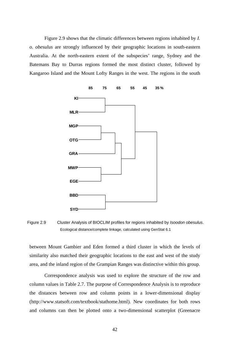
42

Figure 2.9 shows that the climatic differences between regions inhabited by I.

o. obesulus are strongly influenced by their geographic locations in south-eastern

Australia. At the north-eastern extent of the subspecies’ range, Sydney and the

Batemans Bay to Durras regions formed the most distinct cluster, followed by

Kangaroo Island and the Mount Lofty Ranges in the west. The regions in the south

between Mount Gambier and Eden formed a third cluster in which the levels of

similarity also matched their geographic locations to the east and west of the study

area, and the inland region of the Grampian Ranges was distinctive within this group.

Correspondence analysis was used to explore the structure of the row and

column values in Table 2.7. The purpose of Correspondence Analysis is to reproduce

the distances between row and column points in a lower-dimensional display

(http://www.statsoft.com/textbook/stathome.html). New coordinates for both rows

and columns can then be plotted onto a two-dimensional scatterplot (Greenacre

KI

MLR

MGP

OTG

GRA

MWP

EGE

BBD

SYD

85 75 65 55 45 35 %

Figure 2.9 Cluster Analysis of BIOCLIM profiles for regions inhabited by Isoodon obesulus.

Ecological distance/complete linkage, calculated using GenStat 6.1

http://www.statsoft.com/textbook/stathome.html

43

1984). In such plots, the statistical distances between row points (the climatic

parameters from BIOCLIM) can be interpreted, as can the distances between column

points (mean values for 34 BIOCLIM parameters for each region), but not the

distances between row points and column points

(http://www.statsoft.com/textbook/stathome.html).

Correspondence Analysis revealed further information about the climatic

relationships between regions. When the regions were plotted against the first and

second axes calculated by Correspondence Analysis, their CA coordinates aligned

with their geographic coordinates. Kangaroo Island and the Grampian Ranges were

exceptions, possibly due to their respective maritime and continental climatic

regimes, compared to other regions inhabited by I. o. obesulus. These results indicate

that the axes reflect latitudinal and longitudinal climatic gradients, which may relate

to moisture (CA Axis 1) and temperature (CA Axis 2). Regions in the north-east

would have less extreme variations in moisture and temperature due to their

proximity to the subtropics than regions in the south and west, which would be

expected to have greater seasonal variation for these variables.

-0.25

-0.15

-0.05

0.05

0.15

0.25

0.35-0.5-0.4-0.3-0.2-0.100.10.20.30.40.50.6

ki mlr

mgp

gr

og

mp ege

bbd

s

15

18

3130

34

33

8

17

24

12

25

9

6

19

23

1316

28

20

11

2722

1

1021

26

4

72

5

353229

CA Axis 1 (85.66%)

CA

Axis

2 (1

0.29

%)

3

1. Annual Mean Temper ature 10. Mean Temperatur e of Warmest Qtr 19. Precipitation of Coldest Qtr 28. Annual Mean Moisture Index2. Mean Diurnal Range 11. Mean Temperatur e of Coldest Qtr 20. Annual Mean Radiati on 29. Highest Period Moisture Index3. Isothermality 12. Annual Precipitation 21. Highes t Period R adiation 30. Lowest Period M oisture Index4. Temperature Seasonality 13. Precipitation of Wettes t Period 22. Lowest Period R adi ation 31. Moisture Index Seasonality5. Max Temperature of Warmest Period 14. Precipitation of Driest Period 23. R adiation Seasonality 32. Mean Moisture Index of High Qtr6. Min Temperature of Col dest Period 15. Precipitation Seasonality 24. R adiation of Wettest Qtr 33. Mean Moisture Index of Low Qtr7. Temperature Annual R ange 16. Precipitation of Wettes t Qtr 25. R adiation of Driest Qtr 34. Mean Moisture Index of War m Qtr8. Mean Temperature of Wettest Qtr 17. Precipitation of Driest Qtr 26. R adiation of War mest Qtr 35. Mean Moisture Index of C old Qtr9. Mean Temperature of Driest Qtr 18. Precipitation of Warmes t Qtr 27. R adiation of C oldest Qtr

Figure 2.10 Correspondence Analysis of BIOCLIM profiles for regions inhabited by Isoodon obesulus.


44

2.4 Discussion

2.4.1 Distribution and Fragmentation of Isoodon obesulus

By looking at one subspecies, this analysis shows that the fragmented continental

distribution of I. obesulus has been influenced by climate, geology and vegetation.

Over this natural pattern of fragmentation, human-induced fragmentation has been

superimposed since 1788, thus the fragmented distribution of I. o. obesulus in south-

eastern Australia is analogous, but at a finer scale, to the fragmented distribution of

the species in Australia (Figure 1.3).

The prediction showed that vegetation suitability was probably not a major

influence on the species’ fragmented continental distribution in 1788 compared to

climate suitability. The 1988 vegetation suitability map showed that considerable

change occurred over 200 years, and it is obvious even at this coarse scale of

analysis that native vegetation clearance has contributed to the fragmented

distribution of I. obesulus. Much of this land has been cleared for agriculture but the

effects of urbanization can also be seen at this scale, particularly near Adelaide and

Melbourne.

The models indicate that continental scale habitat fragmentation has isolated

regional populations of I. obesulus for more than two centuries and probably much

longer, indeed long enough to influence their evolutionary development. Close et al.

(1990) and Pope et al. (2001) hypothesised that recent gene flow occurred between

geographically distant subspecies of I. obesulus because genetic similarities between

widely dispersed groups indicate that the species has undergone a recent contraction

in its continental distribution relative to the geologic time scale. Climate change and

sea level rise are potentially obvious causes and support for such a view is given by

the presence of I. o. affinis on Tasmania and I. o. nauticus on Nuyts Archipelago.

Even if the five subspecies of I. obesulus had a prior continuous distribution it is

likely that some genetic variation would have existed between populations in

different geographic regions. Within the distribution of the subspecies I. o. obesulus,

it has been observed by Close et al. (1990) and Adams (in Maxwell et al. 1996) that

genetic differences on either side of the lower Murray River valley and Coorong

45

exist, which suggests that these physiographic features have acted as biogeographic

barriers for long enough to cause genetic divergence. Habitat suitability mapping

techniques for all five subspecies in the I. obesulus group may provide further clues

as to why and when the species’ distribution initially became fragmented.

2.4.2 Influence of Climate, Geology and Vegetation

It is clear from the results that each of the three variables performed differently, and

yet the habitat suitability models assumed that climate, geology and vegetation had

an equally weighted influence over the distribution of I. o. obesulus. These three

variables are not mutually exclusive, though in some situations they reinforce one

another. Vegetation patterns at a continental scale are strongly influenced by climatic

and geologic interactions. Likewise, topographic uplands and mountain ranges are

influenced by geologic substrate and together they produce distinctive regional

bioclimates.

Of the three variables examined, climate suitability provided the best model

to explain the fragmented continental scale distribution of I. obesulus and this has

implications for the distribution of the species under future climate change scenarios.

For instance, Brereton et al. (1995) modelled the range of I. o. obesulus in Victoria

under present climate and six enhanced greenhouse scenarios and found that its

distribution could shrink by up to 67%.

A broad range of physiographic phenomena are encompassed by the

distribution of I. o. obesulus but the subspecies is most frequently found on

sedimentary rocks and sandy, weathered regolith. In Victoria, Menkhorst and

Seebeck (1990 p 55) observed that I. o. obesulus is “an animal of the coastal or

fluviatile plains although populations exist in the Grampian Ranges and Dandenong

Ranges.” The volcanic plains of western Victoria fragment the distribution of I. o.

obesulus and the Hawkesbury River in New South Wales marks its northern limit

(Dixon 1978). The lower Murray River valley has also been identified as a point of

genetic divergence for I. obesulus (Adams in Maxwell et al. 1996) but until now it

has not been clear why geologic and topographic features fragment the subspecies’

distribution, for example the La Trobe Valley and the western volcanic plains of

Victoria. The most likely explanation, however, is a combination of climate, geology

46

and vegetation.

In addition to the interaction of these natural factors, fragmentation results

from human activities that lead to land cover change that is so obvious when

comparing the 1788 and 1988 vegetation suitability maps. Even though the 1788

vegetation map provides a natural base map, human-induced changes in vegetation

prior to that time are not incorporated into the model. Since 1788, many of the

regions inhabited by I. obesulus have been cleared and heavily populated due to their

suitability for agriculture, urban settlement and forestry. In a relatively short period

of time, the habitat of I. obesulus has had extensive human-induced fragmentation

imprinted over its naturally fragmented pattern that was formed by climate, geology

and vegetation over a much longer time.

The output from the equally weighted combination of climate, geology and

vegetation was heavily influenced by climate, which is clearly an important factor in

determining the suitability of habitats for I. obesulus at a continental scale. What

influence climate has on the distribution at the regional scale and what other factors

become important are examined in Chapter 3 where habitat fragmentation is

analysed at a higher resolution in the south-east of South Australia.

47

CHAPTER 3 REGIONAL SCALE DISTRIBUTION OF ISOODON OBESULUS

3.1 Isoodon obesulus in the South East of South Australia

This chapter investigates the distribution of I. obesulus in south-eastern region of

South Australia (Figure 3.1). The ‘South East’ is the South Australian vernacular for

this area (Tyler et al. 1983) and it has been recognised as a distinct physiographic

region for many generations, first by Aboriginal people (the Bunganditj) then

European settlers (Pretty et al. 1983). The South East also represents a distinct region

within the broader Kosciuszkan biogeographic province and the pre-European fauna

of the South East was at the western limit of the south-eastern Australian temperate

fauna, along with that found on Fleurieu Peninsula and Kangaroo Island (Aitken

1983).

Figure 3.1 shows that all occurrence records of I. obesulus in the South East

come from south of a line between Penola and Beachport, except for subfossil

records from Naracoorte Caves and a sand dune located between Robe and

Beachport. These specimens indicate that the species once occurred further to the

north and west, which is supported by the continental scale prediction of 1788

habitat suitability (Figure 2.8a), although how far north and west is unknown. The

South Australian Museum catalogued its first specimen of I. obesulus from the South

East in 1927 (specimen number M02326). Specimens were then uncommon until

wildlife surveys were conducted across the region between 1980 and 1991, with

some specifically targeting I. obesulus (Paull 1993, 1995). These surveys found that

I. obesulus was restricted to less than 30 patches of remnant native vegetation

totalling approximately 7000 ha (Figure 3.2).

48

A

M

S

MosquitoReedy Ck

Ck

Figure 3.1 The South East of South Australia with historical records of Isoodon obesulus.

Drainage lines are included. The inset shows the location of the South East of South Australia (shaded) relative to Adelaide (A), Melbourne (M) and Sydney (S).

49

N

remnants with records

other remnant patches

0 50 km

Figure 3.2 Remnant native vegetation associated with accurate and reliable records of Isoodon obesulus.

50

3.1.1 The Study Area

a. Climate

The relevance of climate to I. obesulus at the continental scale was made clear in

Chapter 2 but whether climate contributes to habitat fragmentation at the regional

scale is uncertain. Paull (1993) did, however, observe that the distribution of I.

obesulus in the South East of South Australia was generally associated with 650-850

mm rainfall isohyets. The South East has a cool, moist climate with long mild

summers (Laut et al. 1977). Mean annual rainfall increases southwards (Figure 3.3a)

because of “the increasing oceanic origin of the rain-bearing winds as their passage

becomes less affected by the Yorke and Eyre peninsulas” to the west (Penney 1983 p

85). Precipitation decreases with distance from the coast and variations in mean

annual rainfall arise from the Mt Burr Range, which influences the south of the

region, and the Naracoorte Range in the east (Penney 1983).

a b

Figure 3.3 a Annual mean rainfall and b temperature of the South East.

source: Penney (1983) Figs 1 and 6

51

Mean annual temperature across the region displays a similar pattern to

annual rainfall (Figure 3.3b) whereby a latitudinal effect exists with mean annual

temperature decreasing in a southward direction. Coastal locations have higher mean

annual temperatures than areas immediately inland because of the thermal lag of the

Southern Ocean (Penney 1983). Further inland, continental locations have relatively

extreme maxima and minima temperatures.

b. Geology and hydrology

At the continental scale, various physiographic features were identified in Chapter 2

as having an influence over the fragmented distribution of I. obesulus. At a regional

scale, I. obesulus in the South East exists on a substrate of horizontally bedded

limestone, which is expressed by minimal topographic relief of the surface. Rivers

potentially fragment the species’ continental distribution but in the South East there

are no major rivers; there are, however, lakes and wetlands in the region that may

cause fragmentation at a finer scale.

The basement rock of the South East is granite of Ordovician and Silurian

age (Harris 1983, Twidale et al. 1983) and it is exposed in small outcrops in the

north (Figure 3.4). Over these granitic rocks lie layers of Tertiary limestone which

were deposited as marine sediments in the Otway Basin of the Australian Southern

Rift System while Australia rifted from Antarctica during the Late Cretaceous and

throughout the Tertiary (Morton 1990). Isostacy and faulting during the Tertiary are

both evident in the region; the general plane of the land surface tilts down to the

north and the Kanawinka Fault in the east and the Mt Burr Range 25 km NNW of Mt

Gambier were produced by block faulting (Sprigg 1952). During the late Pleistocene

and into the Holocene, volcanoes were active throughout the southern parts of the

South East, with the principal centres being located along the Mt Burr Range, within

the Mt Gambier complex and south of Mt Gambier at Mt Schank (Sheard 1983).

Marine transgressions during the Tertiary and Pleistocene have formed a prograding

series of 13 geomorphically and 21 stratigraphically distinct, subparallel strandlines

across the broad coastal plain between south-western Victoria and the mouth of the

Murray River in South Australia. Low-lying interdunal corridors of lagoonal and

saline lacustrine origin separate the carbonate dune ranges that have resulted from

52

sea level change related to climate change (Schwebel 1983).

The South East is renowned for having highly productive limestone aquifers,

no rivers and only a few minor creeks (Holmes and Waterhouse 1983). Where

surface water does exist, it is principally in the form of lakes and swamps, which

may potentially fragment the distribution of I. obesulus. These include fresh and salt

lakes, shallow coastal lagoons, swamps, and lakes such as Lakes Eliza, St Clair,

George and Bonney. Away from the coast, Blue Lake, Browns Lake, Valley Lake

and Leg-of-Mutton Lake occur in craters in the Mt Gambier volcanic complex and

Lake Edward and Lake Leake occupy craters in the Mt Burr Range. Karstic lakes,

such as Little Blue Lake and Hells Hole, are found in dolines or cenotes in the south

of the region. Ephemeral lakes and swamps fill during wet years and come to

Figure 3.4 Physiographic and geological features of the South East.

source: Sprigg (1952) Fig. 4, p. 21.

53

dominate landscapes such as the extensive Dismal Swamp. They typically hold water

less than 1 m deep and dry up each summer (Allison and Harvey 1983). Swamps of

the region have three origins: 1) those developed in shallow karst depressions, such

as Marshes Swamp; 2) the Dismal Swamp, thought to have formed in palaeochannels

of the Glenelg River (Sprigg 1952, Allison and Harvey 1983); and 3) swamps

formed where drainage has been impeded by the low relief of the area (Allison and

Harvey 1983). Many large swampy areas have been drained by a network of E-W

tending channels (Figure 3.1) that were cut during the last century but are still being

developed (Taffs 2001).

c. Landforms and soils

It has been observed that I. obesulus prefers certain soil types, particularly sandy

textured soils (Emison et al. 1975, Menkhorst and Seebeck 1990, Opie et al. 1990).

In the study area there is a strong spatial relationship between soils and landforms.

Associated with the geologic units, landform systems have been mapped which

comprise dunes, interdunal plains, undulating plains and volcanic landscapes

(Blackburn 1959, 1983, Laut et al. 1977, Stephens et al. 1941). Soil groups of the

region are, likewise, closely associated with the landform systems (Figure 3.5).

Active coastal dune systems have deep, calcareous, yellow-grey soil horizons while

inland, consolidated calcareous dune systems have shallow, alkaline, reddish soils. In

places, unconsolidated siliceous sand dune systems and sand sheets overly

consolidated calcareous dunes and inter-dunal plains. Their soils are well-drained,

deep and neutral with a yellow-grey, bleached A2 horizon (Laut et al. 1977).

Interdunal plains have uniform clay and duplex soils that limit permeability of water

and induce winter flooding. Interdunal plains on the lee side of coastal dunes often

have shallow, well-drained, alkaline, black uniform loams over shell beds. On the

more elevated parts of interdunal plains, deep, alkaline, imperfectly drained, duplex

soils are found; the surface horizon is sandy with a bleached lower portion, over a

yellow-mottled clayey sub-horizon. The lower-lying parts of the interdunal plains

have deep, alkaline, poorly drained, cracking clays, often associated with swamps

(Laut et al. 1977). Undulating plains are dominated by yellow mottled duplex soil.

On undulating plains where unconsolidated sand dunes and sand sheets occur,

54

yellow-grey siliceous sands are found and in depressions there are black cracking

clays (Laut et al. 1977). The volcanic landscapes of the south possess hills, volcanic

cones and plains. The hills have deep imperfectly drained, acid, bleached siliceous

sand over a yellow hardpan. Older volcanic cones in the Mt Burr Range have deep

acid brown earths and younger cones at Mounts Gambier and Schank have deep,

neutral, brown, uniform loamy soil. Consolidated dunes occur on ash-covered or

limestone plains; they have shallow, alkaline, well-drained, red sandy soils (Laut et

al. 1977). Based on previous observations of habitat use by I. obesulus, it was

expected that these diverse landforms and soils would be important variables for

explaining the fragmented regional distribution of the species.

55

N

0 25 km

Calcareous soils

Cracking clay soils

Sand over clay soils

Deep sands

Highly leached sands

Shallow soils on rock

Wet soils

Volcanic ash soils

Rock

Water

Deep uniform to gradational soils

Shallow soils on calcrete or limestone

Gradational soils with highly calcareous lower subsoils

Deep loamy texture contrast soils with brown or dark subsoils

Hard red-brown texture contrast soils with highly calcareous lower subsoils

Figure 3.5 Soil Groups of the South East.

56

d. Vegetation

Throughout its continental distribution, I. obesulus has been recorded in a wide range

of vegetation types (Tables 2.2 and 2.5) but not all of them are present in the South

East. Furthermore, many types of vegetation that do occur in this region are not

suitable for I. obesulus. The pre-European vegetation of the South East was closely

associated with geologic, landform and edaphic units (Figure 3.6) and owing to the

physiographic complexity of the region, the diversity of flora was great (Lange

1983). The most widespread community was Eucalyptus leucoxylon woodland,

which covered 19% of the region and was found mostly in the north (Figure 3.6). It

was associated with shallow soils on calcrete or limestone and to a lesser degree with

sand over clay soils and deep sands (Figures 3.5 and 3.6). Eucalyptus baxteri open

forests and woodlands grew throughout the region and occupied 18% of the land,

generally on sandy soils associated with unconsolidated siliceous dunes. Melaleuca

halmaturorum covered 12% of the region and was generally found growing on

poorly drained calcareous soils of the interdunal corridors. Besides the relationships

between vegetation and soils, climatic influences were evident in the distribution of

the pre-European vegetation. Communities adapted to more arid conditions occurred

in the north, for example areas of mallee dominated by Eucalyptus behriana, E.

diversifolia, E. odorata and E. rugosa. The remaining communities included

sedgelands, grasslands, heathlands, shrublands, woodlands and open forests

dominated by species adapted to the considerable variations in climate, soil and

drainage found throughout the region.

Most of the native vegetation of the South East was cleared during the 1900s

(Dendy 1985, Dodson 1975, Lange 1983) and this has had serious implications for I.

obesulus, which will be described later in the thesis. Large areas were cleared after

the Second World War when agriculture and softwood forestry were expanding but

clearing ceased in the 1980s when State legislation halted further destruction of

native vegetation (South Australian Vegetation Retention Act 1980). Today, 13% of

the region is covered by native vegetation (Croft et al. 1999), much of which occurs

as degraded remnants surrounded by cropland, pasture and pines (Figure 3.7).

As a consequence of this clearance history, the vegetation classifications used

in Figures 3.6 and 3.7 are difficult to compare. Some communities are now gone

57

while others have been introduced to the region (Croft et al. 1999). Eucalyptus

viminalis, for example, once covered almost 5% of the region but is now so rare that,

at this scale, it can only be mapped in association with E. ovata. Together they

comprise a mere 0.6% of the remaining native vegetation in the South East (Figure

3.7). It is interesting to note that some communities have increased since European

settlement, such as Banksia ornata shrublands (Figures 3.6 and 3.7), and a detailed

comparison of change in vegetation throughout the study area based on these maps

can be found in Carruthers et al. (1999).

The most widespread vegetation type today is Eucalyptus baxteri woodland,

which comprises 14% of the present native vegetation cover and is scattered

throughout the region (Figure 3.7). Banksia ornata shrubland is the next most widely

distributed community (12%), occurring on sandy soils in the north. Melaleuca

brevifolia shrublands occupy wet areas in the north and contribute a total of 11% of

the remnant vegetation while Eucalyptus diversifolia mallee woodlands comprise

nearly 11% of the native vegetation and occur on infertile sandy soils in the north

and west of the region. Much of the remnant native vegetation is adapted to poor

soils and poorly drained sites, which have not been cleared. As a consequence, the

communities remaining in the South East are an incomplete representation of the

ecosystems that once existed and this change is relevant to the occurrence of I.

obesulus because some of the habitats that it once occupied in the South East may

now be gone.

This detailed description of climate, geology, hydrology, landforms, soils and

vegetation of the South East suggests that different factors exist at a finer scale than

the continental scale which could combine to fragment habitat within a region. This

has implications for the choice of modelling variables described in the following

sections of Chapter 3 and again in Chapters 4 and 5 when the study shifts to the local

scale.

58

N

0 25 km

Banksia marginata/B. ornata

Eucalyptus baxteri

Eucalyptus camaldulensis

Eucalyptus leucoxylon

Eucalyptus ovata

Eucalyptus viminalis

Gahnia trifida/G. filum

Granite/salt pan/clay pan

Leptospermum continentale/L. lanigerum

Mallee

Melaleuca gibbosa/M. lanceolata

Melaleuca halmaturorum

Other Eucalyptus species

Other associations

Wetlands and lakes

Figure 3.6 Pre-European vegetation of the South East.

Department of Housing and Urban Development (1996)

Mallee species include Eucalyptus behriana, E. diversifolia, E. odorata, E. rugosa. Other Eucalypts include Eucalyptus largiflorens, E. microcarpa, E. porosa, E. willisii.

Wetlands and lakes include floating water plants, perennial lakes, Phragmites australis, Typha domingensis, swamp. Other associations include Acacia longifolia, Allocasuarina leuhmannii, Allocasuarina verticillata, Baumea juncea, Halosarcia spp., Selliera

radicans, Olearia axillaris, Leucopogon parviflorus, Poa spp., Stipa spp. Spinifex sericeus, Themeda triandra.

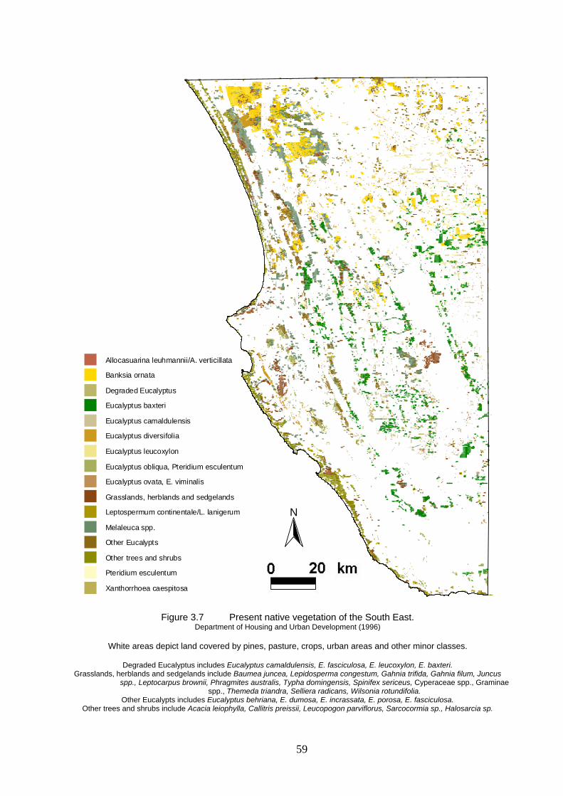
59

N

0 25 km

Allocasuarina leuhmannii/A. verticillata

Banksia ornata

Degraded Eucalyptus

Eucalyptus baxteri

Eucalyptus camaldulensis

Eucalyptus diversifolia

Eucalyptus leucoxylon

Eucalyptus obliqua, Pteridium esculentum

Eucalyptus ovata, E. viminalis

Grasslands, herblands and sedgelands

Leptospermum continentale/L. lanigerum

Melaleuca spp.

Other Eucalypts

Other trees and shrubs

Pteridium esculentum

Xanthorrhoea caespitosa

Figure 3.7 Present native vegetation of the South East.

Department of Housing and Urban Development (1996)

White areas depict land covered by pines, pasture, crops, urban areas and other minor classes.

Degraded Eucalyptus includes Eucalyptus camaldulensis, E. fasciculosa, E. leucoxylon, E. baxteri. Grasslands, herblands and sedgelands include Baumea juncea, Lepidosperma congestum, Gahnia trifida, Gahnia filum, Juncus

spp., Leptocarpus brownii, Phragmites australis, Typha domingensis, Spinifex sericeus, Cyperaceae spp., Graminae spp., Themeda triandra, Selliera radicans, Wilsonia rotundifolia.

Other Eucalypts includes Eucalyptus behriana, E. dumosa, E. incrassata, E. porosa, E. fasciculosa. Other trees and shrubs include Acacia leiophylla, Callitris preissii, Leucopogon parviflorus, Sarcocormia sp., Halosarcia sp.

60

3.2 Methods

The method presented in Chapter 2 for modelling the distribution of I. obesulus at a

continental scale was repeated in this chapter when analysing its regional scale

fragmented distribution in the South East. The continental scale prediction of climate

suitability (Figure 2.5c) was used for this analysis and combined with digital maps of

soils, pre-European vegetation and present vegetation, discussed in detail in the

preceding sections.

3.2.1 Selection of Modelling Records

To develop habitat suitability weightings, 113 records were selected from Appendix

A1 and compared to maps of Soil Groups, Common Soils, Pre-European Vegetation

and Present Vegetation (Figure 3.8). The age distribution of the records was: three

subfossil records of unknown age, one record from the period 1927 to 1971, 27

records from 1979 to 1989 and 82 records from 1990 to 1997. Records were chosen

that were a minimum distance of 250 m apart and where two or more records

Figure 3.8 Records used to model the distribution of Isoodon obesulus at a regional scale.

61

occurred at the same location, only the most reliable one was selected. The estimated

horizontal error of the chosen records ranged from 10 m to 1000 m and averaged 193

m. Excluding the three subfossil records, five records had an estimated horizontal

error of 1000 m and 81 records had accuracies ≤ 200 m.


The BIOMAP prediction of continental scale climate suitability for I. o. obesulus

from Chapter 2 was used in this chapter to create regional scale habitat suitability

maps. The climate suitability map (Figure 2.5c) was chosen because it included a

prediction of the subspecies’ entire climatic niche based on records from all regions

that it inhabits (Figure 2a) and it highlighted areas predicted by BIOMAP using

records from the Mount Gambier to Portland region (Figure 2.5b).

3.2.3 Soil Suitability Classification

A high resolution soil map was available and it was used to investigate the regional

scale relationships between I. obesulus and soil substrate. The soil suitability map

was based on the dataset Soil Landscape Units of the South East of South Australia,

which was supplied by Primary Industries SA. This GIS dataset contains 41 soil

landscape attributes including Soil Group (Figure 3.5) and Common Soils. Soil

Group was an obvious choice for modelling because it encompassed aspects of many

other available soil attributes such as fertility, structure, water holding capacity,

flooding potential and rockiness. However, within each Soil Group polygon, sub-

classes of the most Common Soils were mapped. Comparing I. obesulus records with

the Common Soils map showed that many of these subclasses contained no records.

A weighting scheme was therefore developed for both Soil Groups and Common

Soils and the two weighted soil maps were combined by addition. In this way, the

Common Soil classes associated with the most records were given the heaviest

weight and Common Soil classes with no associated records were given intermediate

weights if they occurred within suitable Soil Groups. Soil Groups associated with no

modelling records received the lowest soil suitability indices.

62

3.2.4 Vegetation Suitability Classification

The dataset of I. obesulus occurrence records was not contemporaneous with either

of the vegetation maps but there was little that could be done about that other than to

rely on the general pattern of vegetation selection revealed by the records. To lend

support to the weighting system for both maps, previous research was called upon

including the information summarised in Table 2.2. An attempt was made to use the

same weights for vegetation types appearing on the pre-European vegetation and

present vegetation maps but it was difficult in the case of E. viminalis and E. ovata.

In the pre-European vegetation classification, the two species were allocated to

separate classes but in the present vegetation map the two species were grouped into

one class. Likewise, E. obliqua was grouped with E. baxteri +/- E. fasciculosa +/- E.

viminalis in the pre-European settlement vegetation map but not in the present

vegetation map, so different weights had to be applied for the species in each map.

3.2.5 Pre-European and Present Habitat Suitability Mapping

To predict habitat suitability for I. obesulus in the South East, two map calculations

were made by adding the pre-European and present vegetation suitability maps to the

climate and soil suitability maps. As in Chapter 2, climate, soil and vegetation were

given equal weighting. The output from each calculation was reclassified into ten

equal-interval habitat suitability indices. Change in habitat suitability was

determined by comparing the pre-European and present habitat suitability maps.

Finally an assessment was made of the nature of land cover changes that have

influenced the distribution of I. obesulus habitat. By doing so, it was possible to

determine what the relative impacts have been of establishing pine plantations

compared to pasture and cropland. To validate the model, the prediction was

compared against the known distribution of I. obesulus habitat in the South East

based on field surveys (Figure 3.2).

63

3.3 Results


Figure 3.9 shows that the distribution of I. obesulus within the South East of South

Australia is not likely to be fragmented by climate, based on the climate suitability

map of this region made at a continental scale in Chapter 2. Developing a higher

resolution, regional bioclimatic prediction for I. obesulus was considered for this

Figure 3.9 Suitability of climate for Isoodon obesulus in the South East.

64

study but not pursued due to scale limitations in the climate surfaces of BIOCLIM

and the network of meteorological recording stations. Figure 3.9 does not indicate

fragmentation but it does indicate a gradient of climate suitability for I. obesulus,

which attenuates northward. The highest suitability indices occurred from the Mt

Burr Range towards the south-east corner of the study area. Prominent areas of low

climate suitability for I. obesulus were predicted immediately inland from Rivoli Bay

and again due east of there, adjacent to the border of the study area (Figures 2.5a and

3.9). Figure 3.3a of mean annual rainfall in the South East shows these two areas lie

between the 700-750 mm isohyets.

3.3.2 Soil Suitability

The greatest weight for the map variable Soil Group was given to the three classes

shallow soils on calcrete or limestone, highly leached sands and sand over clay soils

(Table 3.1) because all except 13 of the modelling records fell into those soils. The

other 13 records corresponded to the classes of wet soils, deep sands, volcanic ash

soils and deep loamy texture contrast soils with brown or dark subsoils and they

were given a lower weight of either 2 or 3. The remaining eight map classes had no

records associated with them and were given a weight of 1 except for rock and water,

which were given 0. For Common Soils in these Soil Groups, the heaviest weight (5)

was given to three classes associated with the greatest number of I. obesulus records:

highly leached sand, thick sand over clay and shallow loam over red-brown clay on

calcrete. Another ten Common Soil classes associated with smaller numbers of

records were given weights between 2 and 4, while classes with no records were

given a weight of 1, except rock and water which were weighted 0.

Figure 3.10 shows the suitability maps for Soil Groups and Common Soils

after being reclassified according to the weights in Table 3.1, as well as the soil

suitability map created by combining the previous two layers. In Figure 3.10a, Soil

Groups with a weight >2 occur throughout most of the study area and approximately

55% of the land was mapped as having a Soil Group weight of 5. Notable areas with

weights <3 included cracking clay soils in the vicinity of Bordertown and deep

uniform to gradational soils and gradational soils with highly calcareous lower

subsoils. Deep sands were prominent between Bordertown and Naracoorte with a

65

weight of 2 and volcanic ash soils were mapped near Mt Gambier, also with a weight

of 2. Rock and water (perennial lakes) with weights of 0 were located along the

western margin of the study area.

The Common Soil map (Figure 3.10b) was conservative in its prediction of

soils for I. obesulus as only 15% of the study area was mapped with a Common Soil

suitability index equal to 5. Common Soils within the Soil Group classes shallow

soils on calcrete or limestone, highly leached sands and sand over clay soils were

weighted to emphasize sandy and loamy textured, non-calcareous and well-drained

surface horizons. As a result, large areas of clayey textured, calcareous and poorly

drained soils mapped as having a weight equal to 5 in Figure 3.10a were mapped in

Figure 3.10b with a lower weight. Other differences between Figures 3.10a and

3.10b included areas in the west and north-west, which were weighted 3 in the

former map and 1 in the latter.

The soil suitability map (Figure 3.10c) predicted that 23% of the study area

has soil suitability in the range of 9 to 10, which occurs predominantly in the south,

although other highly suitable areas associated with Pleistocene dune ranges were

mapped all the way to the northern boundary. Between these areas, soils with lower

suitability were mapped, indicating that the pre-European distribution of I. obesulus

was likely to be fragmented by substrate variation and its control over vegetation

patterns.

66

Table 3.1 Soil suitability weights. SOIL ATTRIBUTE N recs % recs % area ratio SIsoil group (B) Shallow soils on calcrete or limestone 34 30.1 30.1 1.0 5 (I) Highly leached sands 34 30.1 4.1 7.4 5 (G) Sand over clay soils 32 28.3 20.1 1.4 5 (N) Wet soils 7 6.2 8.1 0.8 3 (H) Deep sands 3 2.7 19.5 0.1 2 (O) Volcanic ash soils 2 1.8 1.2 1.4 2 (F) Deep loamy texture contrast soils with brown or dark subsoils 1 0.9 5.9 0.2 2 (E) Cracking clay soils - 3.0 1 (M) Deep uniform to gradational soils - 2.2 1 (C) Gradational soils with highly calcareous lower subsoils - 1.7 1 (W) Water - 1.7 0 (R) Rock - 1.4 0 (A) Calcareous soils - 0.9 1 (D) Hard red-brown texture contrast soils with highly calcareous lower subsoils

- 0.1 1

(L) Shallow soils on rock - <0.1 1 common soil (I1) Highly leached sand 25 22.1 2.6 8.5 5 (G3) Thick sand over clay 20 17.7 9.7 1.8 5 (B6) Shallow loam over red-brown clay on calcrete 19 16.8 2.5 6.9 5 (B3) Shallow sandy loam on calcrete 13 11.5 7.3 1.6 4 (G5) Sand over acidic clay 12 10.6 0.5 20.4 4 (I2) Wet highly leached sand 9 8.0 1.4 5.6 3 (N3) Wet soil (non to moderately saline) 5 4.4 2.2 2.0 3 (B4) Shallow red loam on limestone 2 1.8 1.0 1.7 2 (H3) Bleached siliceous sand 2 1.8 17.2 0.1 2 (N1) Peat 2 1.8 0.8 2.3 2 (O1) Volcanic ash soil 2 1.8 1.2 1.4 2 (F2) Sandy loam over poorly structured brown or dark clay 1 0.9 3.8 0.2 2 (H1) Carbonate sand 1 0.9 1.9 0.5 2 (B7) Shallow sand over clay on calcrete 9.2 1 (G4) Sand over poorly structured clay 8.5 1 (B5) Shallow dark clay loam on limestone 5.8 1 (N2) Saline soil 5.2 1 (B2) Shallow calcareous loam on calcrete 3.1 1 (F1) Loam over brown or dark clay 2.1 1 (E3) Grey or brown cracking clay 1.9 1 (C5) Gradational dark clay loam 1.7 1 (WW) Water 1.7 0 (M2) Deep friable gradational clay loam 1.6 1 (G2) Bleached sand over sandy clay loam 1.4 1 (RR) Rock 1.4 0 (B8) Shallow sand on calcrete 1.2 1 (E1) Black cracking clay 1.0 1 (M4) Deep hard gradational sandy loam 0.6 1 (A6) Gradational calcareous clay loam 0.4 1 (A7) Calcareous clay loam on marl 0.4 1 (H2) Siliceous sand 0.4 1 (A1) Highly calcareous sandy loam <0.1 1 (A4) Deep (rubbly) calcareous loam <0.1 1 (B1)Shallow highly calcareous sandy loam on calcrete <0.1 1 (B9) Shallow clay loam over brown or dark clay on calcrete <0.1 1 (C3) Friable gradational red-brown clay loam <0.1 1 (D2) Loam over red clay <0.1 1 (L1) Shallow soil on rock <0.1 1 (M1) Deep sandy loam <0.1 1

67

a b

c

Figure 3.10 Suitability of soil for Isoodon obesulus in the South East.

a weighted Soil Groups, b weighted Common Soils, c Soil Suitability calculated by adding the weights of the Soil Group and Common Soil maps.

68

3.3.3 Vegetation Suitability

Weights for vegetation are shown in Table 3.2 and were derived in the following

way. Eucalyptus baxteri +/- E. obliqua +/- E. fasciculosa +/- E. viminalis in the pre-

European map and Eucalyptus baxteri +/- Pteridium esculentum in the present map

were associated with the greatest number of records and given the highest weight

(10). Eucalyptus obliqua, Leptospermum continentale and Melaleuca squarrosa are

listed in Table 2.2 as vegetation types known to be used by I. obesulus and were

given relatively high suitability indices in the range of 4 to 6 (Table 3.2). Eucalyptus

ovata and E. viminalis were also given relatively high weights in the range of 5 to 7.

Eucalyptus camaldulensis, Cyperaceae spp./Gramineae spp., E. diversifolia and E.

willisii each had one record (Table 3.2) and were assigned weights of 2 or 3. Isoodon

obesulus has been recorded from E. diversifolia mallee woodland on Kangaroo

Island (Paull 1993) but there was only one subfossil record of the species from E.

diversifolia in the South East. Some vegetation types were over-represented by the

records compared to their area and this was taken into consideration when the

weights were assigned. For example Leptospermum continentale and Eucalyptus

willisii, which only occurred on the pre-European vegetation map, were given

weights of 4 and 3 respectively. Other classes were associated with no records and

were given a weight of 1. An exception was four classes in the pre-European

vegetation map (floating water plants, granite, perennial lake, salt pan/clay pan),

which were given a suitability weight of 0.

The pre-European vegetation suitability map (Figure 3.11a) shows that

vegetation with high suitability for I. obesulus previously existed in the north of the

study area. In fact, vegetation having a suitability index of 10 covered 18% of the

region and 23% of the area had vegetation with suitability indices >6. Relationships

were apparent between the soil suitability map (Figure 3.10) and the distribution of

pre-European vegetation suitability (Figure 3.11a), highlighting, in particular, areas

along dune ranges and sand plains where Eucalyptus baxteri grew on well drained,

sandy and loamy soils. Large tracts of vegetation with suitability indices <6

fragmented the more suitable areas. The vegetation that formerly grew on volcanic

ash soils in the vicinity of Mt Gambier in the south of the study area provides one

example, fragmenting important areas where there was higher vegetation suitability.

69

The change in vegetation suitability shown in Figures 3.11a and 3.11b is

dramatic. Now <2% of the study area has a suitability index of 10 and <3% has

suitability indices >5. Clearly this change is due to the extensive clearance of

preferred vegetation types, especially those associations dominated by E. baxteri and

E. viminalis. However, the relationships between soil and vegetation are indistinct

when the present vegetation suitability map (Figure 3.11b) is compared to the soil

suitability map (Figure 3.10c), not like the pre-European vegetation map.

70

Table 3.2 Pre-European and present vegetation suitability weights. - no data, * not represented in the mapping

Weights were assigned based on the record frequencies and extent of each vegetation class, as well as literature references to habitat use by Isoodon obesulus.

Compared to the pre-European vegetation

map

Compared to the present vegetation

map

Vegetation Association N recs % area ratio N recs % area ratio weight Eucalytpus baxteri +/- E. obliqua +/- E. fasciculosa +/- E. viminalis

80 18.0 3.9 * * * 10

Eucalyptus baxteri +/- Pteridium esculentum * * * 79 14.2 5.4 10Eucalytpus viminalis ssp. cygnetensis 21 4.6 4.0 * * * 7Eucalyptus obliqua, Pteridium esculentum * * * 8 4.5 1.7 6Eucalyptus ovata, E. viminalis * * * 4 0.6 6.5 6Melaleuca squarrosa +/- Eucalyptus ovata * * * 7 0.3 27.2 6Eucalytpus ovata 6 1.8 2.9 * * * 5Leptospermum continentale 3 0.1 22.1 2 0.3 6.7 4Eucalytpus willisii 1 <0.1 89.0 * * * 3Cyperaceae spp., Gramineae spp. * * * 1 1.3 0.7 2Eucalyptus camaldulensis 1 8.0 0.1 1 5.8 0.2 2Eucalyptus diversifolia 1 2.8 0.3 1 10.1 0.1 2Acacia leiophylla * * * - <0.1 - 1Acacia longifolia var. longifolia - <0.1 - - - - 1Allocasuarina luehmannii - 0.9 - - 0.2 - 1Allocasuarina verticillata - 1.9 - - 0.1 - 1Allocasuarina verticillata, Eucalyptus leucoxylon * * * - <0.1 - 1Banksia marginata - 4.7 - * * * 1Banksia ornata - 0.4 - * * * 1Banksia ornata +/- emergent Eucalyptus incrassata * * * - 12.4 - 1Baumea juncea +/- Gahnia trifida * * * - 0.5 - 1Baumea juncea, Chorizandra enodis - <0.1 - * * * 1Baumea juncea, Leptocarpus brownii, Leptocarpus tenax with emergent +/- Melaleuca brevifolia +/- Leptospermum myrsinoides +/- L. coriaceum

* * * - <0.1 - 1

Callitris preissii, Eucalyptus baxteri * * * - <0.1 - 1Degraded Eucalyptus camaldulensis or E. fasciculosa or E. leucoxylon or E. baxteri

* * * - 0.8 - 1

Eucalyptus arenacea * * * - <0.1 - 1Eucalyptus baxteri, Baeckea behrii * * * - 0.1 - 1Eucalyptus behriana +/- E. dumosa * * * - <0.1 - 1Eucalyptus behriana +/- E. dumosa, Melaleuca wilsonii +/- M. uncinata or E. incrassata +/- E. leptophylla

- 6.6 - * * * 1

Eucalyptus dumosa, E. leptophylla * * * - 0.1 - 1Eucalyptus fasciculosa, E. leucoxylon spp. * * * - 0.6 - 1Eucalyptus fasciculosa, Xanthorrhoea caespitosa * * * - 6.1 - 1Eucalyptus incrassata, E. leptophylla +/- Melaleuca uncinata

* * * - 2.3 - 1

Eucalyptus largiflorens - <0.1 - - <0.1 - 1Eucalyptus leucoxylon * * * - 0.1 - 1Eucalyptus leucoxylon +/- Acacia pycnantha * * * - 3.5 - 1Eucalyptus leucoxylon Callistemon rugulosus * * * - <0.1 - 1Eucalyptus odorata - 0.2 - * * * 1Eucalyptus odorata, E. leucoxylon spp. * * * - <0.1 - 1Eucalyptus porosa, E. calycogona swamp complex * * * - <0.1 - 1Eucalyptus rugosa - <0.1 - * * * 1Eucalytpus leucoxylon +/- E. fasciculosa - 19.2 - * * * 1Eucalytpus microcarpa - 1.0 - - 0.2 - 1Eucalytpus porosa - <0.1 - * * * 1

71

Table 3.2 continued

Gahnia filum - 4.9 - * * * 1 Gahnia filum with invading Olearia axillaris * * * - <0.1 - 1 Gahnia filum, Samolus repens * * * - 3.9 - 1 Gahnia trifida - 4.5 - * * * 1 Graminae spp. * * * - 0.1 - 1 Halosarcia spp - 0.1 - * * * 1 Juncus spp., Isolepis spp., Poa spp. complex * * * - 0.2 - 1 Lepidosperma aff. congestum with emergent Gahnia trifida

* * * - 0.1 - 1

Leptocarpus brownii, Baumea juncea * * * - 0.5 - 1 Leptospermum lanigerum - 0.5 - - 0.4 - 1 Leucopogon parviflorus, Acacia longifolia var. sophorae, Olearia axillaris

* * * - 6.8 - 1

Melaleuca brevifolia * * * - 11.1 - 1 Melaleuca brevifolia or Melaleuca uncinata * * * - <0.1 - 1 Melaleuca gibbosa, Hakea rugosa - <0.1 - * * * 1 Melaleuca halmaturorum * * * - 6.4 - 1 Melaleuca halmaturorum or M. brevifolia - 11.7 - * * * 1 Melaleuca lanceolata * * * - 0.3 - 1 Melaleuca lanceolata, Allocasuarina verticillata - 3.1 - * * * 1 Melaleuca uncinata * * * - <0.1 - 1 Muehlenbeckia florulenta - <0.1 - * * * 1 Olearia axillaris, Leucopogon parviflorus - 1.3 - * * * 1 Phragmites australis, Typha domingensis - <0.1 - - <0.1 - 1 Poa spp., Stipa stipoides - <0.1 - * * * 1 Pteridium esculentum +/- emergent Eucalyptus spp. * * * - 0.6 - 1 Sarcocornia sp., Halosarcia sp. * * * - 1.4 - 1 Selleria radicans * * * - <0.1 - 1 Selliera radicans +/- Wilsonia backhousei - 0.8 - * * * 1 Spinifex sericeus, Isolepis nodosa - 0.2 - * * * 1 Spinifex sericeus, Ozothamnus turbinatus, Isolepis nodosa

* * * - 0.1 - 1

Themeda triandra * * * - <0.1 - 1 Themeda triandra, Stipa spp - 0.6 - * * * 1 Typha domingensis * * * - <0.1 - 1 Wilsonia rotundifolia * * * - <0.1 - 1 Xanthorrhoea caespitosa * * * - 0.1 - 1 Xanthorrhoea caespitosa, Leptospermum continentale

* * * - 0.6 - 1

Swamp - <0.1 - * * * 1 Floating waterplants - 0.1 - * * * 0 Granite - <0.1 - * * * 0 Perennial Lake - 1.3 - * * * 0 Salt Pan/Clay Pan - 0.1 - * * * 0 No data * * * - 3.1 - 1

72

3.3.4 Habitat Suitability

The combination of the climate, soil and vegetation suitability maps shown in Figure

3.12 did not predict many places on the pre-European map where habitat suitability

was >7 and most of these areas were in the south where suitable combinations of

climate, soil and vegetation occurred (Figure 3.12a). For the present habitat

suitability map, cells in the model with suitability indices >7 corresponded very

closely with the known distribution of I. obesulus in the South East (Figure 3.2).

With minor exceptions, the model predicted the remnants occupied by I. obesulus

and failed to identify any other areas with habitat suitability >7. From the pre-

Figure 3.11 Suitability of a pre-European and b present vegetation for Isoodon obesulus in the South East.

73

European prediction of habitat suitability, it seems that combinations of vegetation,

soil and climate formerly fragmented the regional distribution of I. obesulus. In the

present habitat suitability map, those natural patterns of fragmentation are barely

recognizable at this scale because human-induced fragmentation is so dominant.

The graph shown in Figure 3.13a compares the area of land that each model

predicted for habitat suitability indices 1-10. A clear trend is visible whereby the area

of land with habitat suitability indices <5 increased while the area with habitat

suitability indices >4 decreased since the time of European colonisation. Figure

3.13b shows the relative area of each index in the pre-European habitat suitability

map and the land cover that now occurs in these areas. Large areas which previously

had low predicted habitat suitability have been converted to pasture and cropland

whereas areas with high predicted pre-European habitat suitability have been

Figure 3.12 Suitability of a pre-European and b present habitat for Isoodon obesulus in the South East.

74

converted to pine. The area of the pre-European habitat suitability map that remained

under native vegetation ranged between 11% and 24% for each of the ten indices.

When the pre-European habitat suitability map was recalculated using masks

of the areas currently under pine plantations (Figure 3.14a) and cropland and pasture

(Figure 3.14b), it was found that pine plantations, although small in area compared to

cropland and pasture, have replaced much of the best habitat for I. obesulus. Figure

3.14c shows that small but important remnants of native vegetation have been

conserved, important because of their high pre-European habitat suitability indices.

0%

10%

20%

30%

40%

50%

60%

70%

80%

90%

100%

1 2 3 4 5 6 7 8 9 10

HSI

Per

cent

are

a of

eac

h ha

bita

t sui

tabi

lity

valu

e

native veg pasture pine

010

0000

2000

0030

0000

4000

0050

0000

6000

0070

0000

8000

00

1 2 3 4 5 6 7 8 9 10

HSI

area

(ha)

PE HSI Pres HSI

Figure 3.13 Change to the area of habitat suitability in the South East.

a Change in the area of habitat suitability between the pre-European and present prediction; and b pre-European settlement habitat suitability indices divided into present land cover classes.

75

Only a small area of habitat with high suitability for I. obesulus remains:

4883 ha are predicted by 1988 HSI values >8 and 13 293 ha by HSI values >7. This

compares with 49 494 ha (HSI >8) and 122 485 ha (HSI >7) respectively in the pre-

European prediction of habitat suitability. Thus, the area of habitat for I. obesulus

with suitability indices >7 was approximately 10 to 15 times greater at the time of

European settlement than at present, based on a comparison of the two predictions.

a b c

Figure 3.14 Change to the distribution of pre-European habitat suitability in the South East.

Areas of the pre-European HSI prediction that are now a pine plantations, b pasture, cropland and minor land cover types, and c native vegetation. Despite covering a smaller area, the establishment of pine plantations appears to

have had a greater impact on I. obesulus habitat than the establishment of pastures.

76

3.4 Discussion

The South East of South Australia represents many regions of Australia that have

been cleared of their native vegetation. Extensive areas have been converted to

pasture, croplands and pine plantations. As a result, the regional scale distribution of

I. obesulus has become highly fragmented since European settlement. Paradoxically

pine plantations appear to have had a greater impact on the distribution of I. obesulus

than pastures and croplands despite their smaller area. This is because pines have

been planted where the best conditions of climate, soil and vegetation occur for I.

obesulus.

The regional scale predictions modelled in this chapter provide information

on habitat suitability that enhances the continental scale analysis of habitat suitability

(Figures 2.8a and 2.8b). Regional scale habitat fragmentation, for example, was not

obvious from the continental scale prediction, and this is shown to apply again in the

following two chapters which deal with habitat fragmentation of I. obesulus at a

finer, local scale. By using higher resolution mapping of floristic associations instead

of vegetation structure, and soils instead of geologic attributes, it was possible to

accurately model the distribution of vegetation remnants occupied by I. obesulus.

There was strong correspondence between vegetation and soils but suitable

vegetation did not always overlap suitable soils. Thus the method of combining soil

and floristic data was advantageous. Even though the climatic suitability map was

generated at a coarser resolution and did not explain the fragmented regional

distribution of I. obesulus, adding it further enhanced the model by emphasizing

remnants in the southern part of the study area.

The pre-European vegetation map (Figure 3.11a) represented vegetation

equivalent to that currently used by I. obesulus because the modelling records were

all post 1971, except three subfossil records. By applying a small weight to mallee

and other classes of vegetation, a conservative prediction was made of the area of

habitat originally available. All evidence, however, suggests that the vegetation types

most heavily weighted in Table 3.2 were formerly and still are the most suitable for

I. obesulus in the South East. One question that arises, has habitat ever been suitable

in the north of the region?

77

If more weight had been placed on classes such as Eucalyptus diversifolia,

the habitat suitability indices would still not have increased greatly northwards

because climate was a limiting factor. Therefore, in order for the prediction of high

habitat suitability for I. obesulus to increase northwards, climatic suitability would

have to change. Given a different pattern of climate suitability in the past, it is

possible that the range of the regional population did once extend northwards

because soils and vegetation were not necessarily constraining factors. As explained

in Section 3.2.2, the climate suitability prediction used for I. obesulus in the South

East incorporated both the continental scale prediction of climatic suitability based

on 323 records (Figure 2.5a) and the regional scale prediction based on 83 records

from Mt Gambier to Portland (Figure 2.5b). The climate suitability map included

areas to the north of the study area that would not have been climatically suitable if

the model was based solely on records from the Mount Gambier to Portland region

(Chapter 2). The climatic prediction used to model the distribution of I. obesulus in

the South East, therefore, indicates that it is unlikely that I. obesulus occurred in the

north of the study area when Europeans first settled.

It is evident that the disjunction between I. obesulus in the South East and the

Mount Lofty Ranges to the northwest has been in place for a long time because

genetic divergence has been noted between the two populations (Section 1.3.2). Gene

flow may have been halted by physical barriers at the lower Murray River valley and

Coorong but climate also appears also to play a role in defining the limits to the

distribution of I. obesulus in the South East. It can be assumed that I. obesulus in the

South East has been separated from the Mount Lofty Ranges for at least 10 000

years. This is presumably the period during which Tasmanian and Nuyts Archipelago

I. obesulus became isolated and subspeciated, although under unique selective

pressures. To obtain a clearer picture of when the two populations became separated,

an attempt could be made to model the bioclimatic distribution of I. obesulus based

on palaeoclimatic estimates but, even if this could be achieved, it would also require

vegetation and soils information that could not be acquired at the required resolution.

Climate change has also been associated with changes to the land area of the South

East, which altered throughout the Quaternary due to repeated marine transgressions

across the coastal plain. Finally, the climatic niche of I. obesulus can not be

78

considered a static phenomenon because species evolve. Climates suitable for I.

obesulus in present times can be presumed to have been suitable at the time of

European settlement but not necessarily at the end of the Pleistocene. Climate change

is likely to influence the distribution and evolution of I. obesulus in the future and

this has implications for the species’ conservation, which is discussed in Chapter 6.

At a practical level, the results presented in this chapter could be used to

guide conservation work for the species by identifying areas with soil and climate

that would be suitable if revegetated. Many of the native vegetation remnants

available to I. obesulus have been disturbed and degraded by wood collection, weed

invasion, animal grazing and fire but these factors are not apparent at the regional

scale of mapping used in this chapter. To isolate such factors, a higher resolution is

required and this is presented in Chapters 4 and 5 where a local scale analysis is

made of the distribution of I. obesulus within native vegetation remnants.

79

CHAPTER 4 LOCAL SCALE I. HABITAT USE BY ISOODON OBESULUS

IN THE SOUTH EAST

4.1 Introduction

In this chapter there is a shift from the regional scale to the local scale when the

distribution of Isoodon obesulus is studied within native vegetation remants in the

South East of South Australia. With the change in scales, there is a change in

methods and geographic information systems (GIS) techniques are used in this

chapter to design a carefully stratified field survey rather than analyse spatial

patterns, although this happens again in Chapter 5 when the spatial distribution of I.

obesulus within remnants is modelled using GIS.

The general distribution of vegetation remnants that contain I. obesulus in the

South East has been analysed in Chapter 3 but the distribution and abundance of I.

obesulus within these remnants is not known. The species has been detected at only a

small number of sites trapped or surveyed for wildlife within these remnants (Paull

1993), suggesting that unknown factors disrupt the continuity of habitat and thus

cause framentation at the local scale. Large areas of potential habitat appear to be

unused by I. obesulus but little else is known about the fine scale distribution or

abundance of the species within the remnants. What is the distribution of I. obesulus

within remnant patches of native vegetation in the South East of South Australia?

Such patches result from the disruption of broader scale continuity of habitat and

therefore represent fragmentation but it is not known if I. obesulus habitat is

fragmented within the remnants and, if so, what factors might cause it.

4.1.1 Habitat Suitability at the Local Scale

For the determination of habitat suitability at the local scale, it was assumed that the

distribution of I. obesulus within native vegetation remnants is influenced by two

main variables, being the availability of food and shelter from predators. Other

factors are potentially very important but they were not the focus of this study. For

example, there is little field-gathered ecological information available on the species’

80

trophic relationships with predators and prey. Likewise, its social interactions with

con-specifics are poorly understood, although it is generally considered to be a

pugnacious and solitary animal (Collins 1973, Heinsohn 1966, Jones 1924, Stoddart

and Braithwaite 1979, Quin 1985a). Instead, habitat variables were chosen on the

basis of their ability to reflect food and shelter resources in I. obesulus habitat, which

are summarised below under the headings soil, vegetation and fire.

a. Soil

The preference of I. obesulus for sandy textured soils, noted in Section 2.2.3, is

unexplained but some relationships can be deduced. The primary foraging niche of I.

obesulus is the soil A-horizon where it digs for the bulk of its food and sites used by

the species display characteristic diggings (Figure 4.1). Friable sandy and loamy

soils should be optimal for the invertebrates that I. obesulus eats because aeration

and drainage would be better for them than in fine textured, compact, poorly aerated

and poorly drained soils. Additionally, hard and rocky soils would be more difficult

for I. obesulus to dig in than sandy soils, requiring the expenditure of greater energy

to obtain food.

b. Vegetation

Apart from a preference for the broad vegetation types described in Chapters 2 and 3,

the structure of vegetation near the ground is important for I. obesulus, an

observation first made by Heinsohn (1966). The species occurs in habitats with mid-

dense to dense ground layer vegetation and is rarely found in areas with sparse

ground cover. Isoodon obesulus builds nests in shallow scrapes using grass, leaves

and litter to produce a mound-like structure that is normally concealed by dense

ground layer vegetation. Some plant species play an important role by providing a

place for I. obesulus to conceal its nests. In the South East, most nests of I. obesulus

are concealed beneath the foliage of Xanthorrhoea australis (Figure 4.2).

81

Figure 4.1 Typical conical digging of Isoodon obesulus.

The depth of the hole is approximately 13 cm. Digging depths of 10-15 cm are typical but diggings >40 cm have been noted in the South East by the author.

Footprints and a tail-drag mark can be seen in the foreground of the freshly created spoil heap. In the South East of South Australia, these diggings can not readily be confused with diggings of other species.

Figure 4.2 Nest of Isoodon obesulus.

The position of this nest is typical of those found in South Australia, because it is beneath the protective cover of a Xanthorrhoea, in this case X. semiplana in the Mount Lofty Ranges. An

Australian 50-cent coin appearing by the recently abandoned nest provides a scale.

82

c. Fire

Fire is considered to be an important factor in determining the distribution and

quality of habitat for I. obesulus. More than two decades ago Braithwaite and Gullen

(1978) and Stoddart and Braithwaite (1979) reached the conclusion that I. obesulus

prefers early successional communities after comparing I. obesulus trapping data

from different sites at Cranbourne, near Melbourne. Relatively high capture rates

were obtained at one site dominated by Leptospermum continentale, which had been

rolled (not burnt) and was regenerating. By contrast, a control site with similar but

relatively mature vegetation produced lower capture rates. Later, Braithwaite (1983)

postulated that vegetation regenerating from fire was likely to sustain a high

diversity of invertebrate food sources for I. obesulus. Based on this evidence,

Stoddart and Braithwaite (1983) and Possingham and Gepp (1993, 1996) interpreted

that I. obesulus is a species amenable to habitat enhancement through deliberate

patch burning to maintain a complex mosaic of regenerating vegetation. Aitken

(1983), however, warned that habitat for I. obesulus in the South East was being

degraded by too frequent burning by the former Woods and Forests Department of

South Australia, a practice that has been continued by the current managers

ForestrySA and which is investigated in detail in Chapter 5. An earlier study by the

author found no significant difference in the trapping rates of I. obesulus in the South

East in vegetation <7 years or >7 years (Paull 1993). Fires within the study area

occur at variable scales ranging from large bushfires that can burn multiple remnants

to small fuel reduction burns within sections of the remnants. Bushfires that

completely burn isolated remnants have been shown to cause the local extinction of

I. obesulus but small fuel reduction burns have not (Thompson et al. 1989).

83

4.2 Methods

To investigate the factors that influence the distribution of I. obesulus within the

native vegetation remnants shown in Figure 4.3, surveys were conducted at 372 sites

during spring in 1998 and 1999. The surveys were stratified so that different habitat

types were sampled in proportion to their area. An additional aim of the sampling

was to allocate at least 1 site per 20 ha per remnant. Habitat units for sampling were

defined by overlaying digital elevation models (DEMs) with vegetation and fire

history maps using ArcView 3.2a. Field surveys were then conducted of a

representative sample of these units to determine the presence/absence and

abundance of I. obesulus diggings and to make observations of relevant habitat

features. To analyse the data, GenStat 6.1 was used to develop six generalized linear

Woolwash

N

0 10 km

never recorded

present

present 1980s, absent 1998/99

present 1990, absent 1998/99

Mt Burr landsystem

Young landsystem

Kays

Windy Hill N

Honan

Grundy

Wandilo

Hacket

Diagonal Rd

The Heath

Byrnes

Paltridges

Wild Dog

Honeysuckle

Whennans

Mt McIntyreMcRosties

Overland Tk

MarshesBurr Slopes

Native Wells

Glencoe RdMt Watch

GowerWindy Hill S

Longs

The Bluff

Figure 4.3 Patches of remnant native vegetation surveyed for Isoodon obesulus in the South East.

Based on Paull (1993, 1995, 1998).

84

models with diggings as the response variable and the habitat features recorded in the

field as the explanatory variables.

4.2.1 Statification of Sampling Units

Habitat units were mapped by combining a DEM of each remnant with thematic

maps of vegetation and fire history. Digital elevation models were created and used

to classify local relief within remnants. As explained in Section 3.1.1, strong

associations exist between elevation, landforms and soils in the study area (Stephens

1957). Vegetation patterns are also strongly influenced by landforms, although some

plant communities in the study area exist on multiple landform types. For example,

Eucalyptus baxteri woodland is the most widely distributed community in the

remnants and it grows on dunes as well as lower-lying plains. Leptospermum

continentale dominates shrubland communities, and it grows in low depressions and

on plains. Other communities, such as reedbeds and sedgelands grow only in

depressions. Maps of fire management blocks and records of the years when each

block was burnt were included in the stratification in order to representatively

sample sites of different regeneration age and fire frequency.

a. Creation of digital elevation models and classification of local relief

Digital elevation models of each remnant were constructed using 10 m interval

contour lines and spot heights, digitised from 1:50 000 topographic map sheets.

Digitised outlines of dune crests and depressions, derived from aerial photographic

interpretation and mapped onto the same 1:50 000 topographic map sheets were also

available and obtained in hardcopy from Ken Grimes (Regolith Mapping). These

dune crests and depressions were also digitised and combined with the contour and

spot height information. An example is illustrated in Figure 4.4 using one remnant,

Woolwash Native Forest Reserve, and the digital elevation models for all remnants

appear in Appendix A4.1. Contours, spot heights, dune crests and depressions were

digitised from the topographic sheets using ERMapper 5.5 and a Summagraphics

digitiser, then imported as *.dxf vector format files into ArcView 3.2a. In ArcView,

point files were created using the vertices of the contour lines and these were merged

with the spot heights from the topographic maps. Estimated spot heights were also

entered between contour lines to produce a smooth interpolation (Figure 4.4a). The

85

surfaces were interpolated to the edge of each remnant using ArcView’s Inverse

Distance Weighted method, an analysis mask and small (5 m) cells (Figure 4.4b).

The next step involved digitising outlines of dune crests and depressions,

which were not represented by the 10 m contours on the 1:50 000 topographic maps

due to their low topographic (<10 m) relief. Shapefiles of dune crests and

depressions (Figure 4.4.c) were rasterised and distance maps were created from dune

crests to the edges of depressions and the edges of remnants. The Map Calculator

was then used to transform the values of the distance maps using [distance.log10cos]

and the results were reclassified into ten equal-interval classes that simulated

elevation surfaces running from dune crests to depressions (Figure 4.4d). The

transformed and reclassified distance maps were added to the elevation maps (Figure

4.4b) using Spatial Analyst’s Map Calculator (Figure 4.4e) and ground truthing

showed that, for the purpose of this study, topographic relief within the remnants was

adequately represented, albeit with horizontal errors up to 100 m and vertical errors

up to 15 m. Although the DEM distorted elevation and assumed cross-sectional

symmetry of dunes, it was found to be effective for mapping minor landforms with

low relief not evident from the 10 m contour information on the 1:50 000

topographic maps.

To stratify the remnants into elevation sampling units, the DEMs were

reclassified by up to four local relief classes, which were defined for each remnant

after identifying major breaks of slope. The elevation values that appear in Appendix

A4.2 were used to reclassify the DEM for each remnant into the following classes:

1000 (low relief, mostly depressions and plains), 2000 (low to intermediate relief,

typically plains), 3000 (intermediate to high relief, low dunes and low hill slopes)

and 4000 (high relief, high dunes and upper hill slopes). The example shown in

Figure 4.4f includes all four relief classes because Woolwash has the greatest range

in elevation of the remnants surveyed. A map of relief classes for all remnants

appears in Appendix A4.3.

86

Figure 4.4 Construction of digital elevation models and stratification of local relief.

a contour and spot height information, b elevation surface interpolated from the contours and spot heights, c dune crests and depressions interpreted from aerial photographs by K. Grimes (Regolith Mapping), d transformed

distance surface calculated from dune crests to edges of depressions, e digital elvation model made by adding Figure 4.4b to 4.4d, and f stratified relief classes based on breaks of slope and landforms (Appendix A4.2).

87

b. Vegetation mapping

Vegetation units for the survey were derived from the Floristic Map of the South

East obtained from the Department of Housing and Urban Development (Figure 3.7).

Vegetation associations mapped in the remnants included three woodland

communities, Eucalyptus baxteri, E. obliqua and E. ovata/E. viminalis complex,

which were assigned the codes 100, 200 and 300, respectively. Shrubland species

Leptospermum continentale, Melaleuca squarrosa and M. brevifolia were grouped as

a fourth class (shrubs 400) and remaining vegetation was classified as

reedbed/sedgeland complex (500) and other (600), which included species of Acacia

and pine mixed with Eucalypts. An example vegetation map for Woolwash Native

Forest Reserve is provided in Figure 4.5 and a vegetation map for all remnants

appears in Appendix A4.4.

N

0 500 m

veg codes100400500600

Figure 4.5 Vegetation sampling units for Woolwash. 100 Eucalyptus baxteri, 400 shrubs, 500 reedbed/sedgeland complex, 600 other

88

c. Fire history mapping

The history of fires within the remnants was mapped by obtaining records dating

from 1957 to 1998 from ForestrySA. Most of the fires in this time have been

deliberately lit by ForestrySA and the former Woods and Forests Department, who

maintained detailed records in unpublished forestry reports. Management fires are

periodically lit in blocks in response to increased fuel load, and vehicle tracks and

firebreaks delineate the blocks, which average approximately 20 ha. Most fires have

been hot and completely burnt the blocks. Records of unsuccessful, partial or

incomplete burns were excluded when compiling the fire data, which were entered

into the attribute table of an ArcView shapefile of the blocks supplied by

ForestrySA. From these data two maps were produced of the remnants, 1) the

number of fires between 1957 and 1998 and 2) the number of years in 1998 since last

burning. Unique values were assigned to fire frequency and fire age classes of these

two GIS themes, which were then overlaid using addition to produce fire sampling

units (Figure 4.6, Appendix A4.5).

Figure 4.6 Fire sampling units for Woolwash.

First digit: number of fires between 1957 and 1998 (0 nil fires, 1 1 fire, 2 2 fires, 3 3 fires, 4 4 fires, 5 5-7 fires). Second digit: age class since last burning (1 <5 years, 2 5-9, 3 10-14, 4 15-19, 5 >19 years).

Example: 34 – burnt 3 times since 1957 but not for 15-19 years.

89

d. Mapping habitat sampling units

The landform, vegetation and fire history maps for each remnant were overlaid by

addition using the Map Calculator in ArcView. This produced 254 different

combinations of relief class, vegetation and fire and these were used as a basis for

sampling across the study area. Figure 4.7 shows the base map used to sample

Woolwash and Appendix A4.6 shows the sampling units for all remnants.

Figure 4.7 Habitat sampling units for Woolwash and site locations. Examples: 1424 - a low lying area with Eucalyptus ovata/Eucalyptus viminalis complex, burnt twice since 1957, the last

time being 15-19 years ago

3133 - an area of intermediate to high local relief with a cover of Eucalyptus baxteri, burnt three times since 1957, the last time being 10-14 years ago.

90

4.2.2 Field-based Site Surveys

At each site, the abundance of I. obesulus diggings was estimated during active

searches walked through 100 m x 100 m quadrats (Figure 4.8). This quadrat area was

chosen because it approximated the minimal size of the home range of I. obesulus as

shown by Lobert (1990). In the field, the quadrat dimension was estimated after

placing a 2 m survey staff at the centre of the site from which the active search was

walked in loops through each quarter of the quadrat for a minimum distance of at

least 300 m.

a. Location

The location of sites within sampling units was determined to a large degree by

accessibility. During the initial site surveys an attempt was made to place sites as

near as possible to the centre of each mapped habitat unit but this was soon found to

be impractical due to the density of understorey vegetation and the difficulty of

movement. This was particularly the case at sites with very dense shrub and ground

layers, which were extremely difficult to walk through without heavily disturbing the

vegetation. Therefore, sites were located as far as practical from the boundaries of

the mapped sampling units and other sites, and it was assumed that the results

obtained from each 1 ha quadrat represented bandicoot digging abundance and

habitat conditions across the whole sampling unit. A snowballing quota approach

100 m

100

m

Figure 4.8 Quadrat dimension and active search pattern.

91

was used for sampling until the desired frequency of 1 site per 20 ha per remnant

was achieved. As the surveys progressed, the habitat units that had previously been

under-sampled were preferentially selected, regardless of the remnants they occurred

in, to maintain near equal proportions in the total sample.

The location of each quadrat was determined using Global Positioning

System (GPS) receivers. At the commencement of the survey, prior to the removal of

Selective Availability from the system, a Trimble GPS unit was used on averaging

mode and >100 readings were taken at the centre of each site. In most instances this

GPS was found to be reliable to within 25 m though occasional unexpected errors

>100 m were observed. Later in the survey, different GPS units were used, including

a Garmin 12XL and Garmin GPSMAP 175 in combination with an Omnistar

differential receiver to provide real time differential sampling with <10 m accuracy.

Validation of a sample of site coordinates in the spring of 2000 using a Garmin eMap

indicated that coordinates collected during the field survey were reliable to within

approximately 25 m.

b. Isoodon obesulus diggings: the response variable

Diggings were used to estimate the presence/absence and abundance of I. obesulus

because they offer a rapid and non-intrusive method (Figure 4.1). Observing foraging

activity is a reliable technique in the South East because other species like the long-

nosed potoroo Potorous tridactylus and eastern long-nosed bandicoot Perameles

nasuta, which make similar diggings, do not occur there. It was assumed that the

presence/absence of diggings indicated the presence/absence of I. obesulus but the

abundance of diggings could not be directly related to the number of individuals

using a site. The abundance of diggings, however, was used as a surrogate measure

for the quality of habitat. Nests and scats were also sought as an indication of the

presence of I. obesulus but they were rarely found. It is very difficult to count the

exact number of diggings at sites inhabited by I. obesulus because of the dense

nature of vegetation, therefore the number of diggings was estimated per 100 m

walked during the active searches and the estimate was made in one of four digging

abundance classes (Table 4.1).

92

Counting diggings was chosen in preference to other methods, such as

trapping, in order to maximise the sample size. Diggings are an obvious sign that I.

obesulus is using a site (Fairbridge et al. 2001) while trapping is not necessarily a

good indicator. Earlier studies by the author indicate that trapping can be conducted

where fresh diggings occur for four consecutive nights without making a capture of I.

obesulus but the following week, several individuals may be captured at the same

site. Radiotelemetry has demonstrated that some individuals are trap-shy while

others habituate to trapping, which further complicates abundance estimates for I.

obesulus (Paull 1993). Estimating the abundance of diggings, therefore, is an

excellent survey method in the study area because diggings are visible for many

months after being formed (Appendix A5).

Diggings indicate the presence of I. obesulus at a site but they can only be

used to infer the abundance of individuals. Quin (1985a) demonstrated that I.

obesulus is an efficient forager that obtains items of food from a high percentage of

the holes it digs and random digging is minimal. In one night, an individual I.

obesulus in captivity was observed to dig 32 holes (Quin 1985a). The mean number

of holes dug by the species in captivity per night, however, was only nine (Quin

1985a). If the approximate number of holes can be estimated, diggings potentially

offer a useful surrogate measure of I. obesulus abundance.

c. Relief, landform, drainage and soil

Table 4.2 summarises the variables collected in the field. Relief and landforms of the

study area were considered to be potentially important for I. obesulus because they

influence site drainage conditions, soil formation and vegetation. The relief class of

each site was taken directly from the base maps (Appendix A4.3) and landforms

were described in the field in three categories, 1) slopes >3o, measured with a

clinometer, 2) plains <3o, and 3) depressions. The drainage class of sites was

Table 4.1 Abundance estimates for Isoodon obesulus diggings. Abundance class Number of diggings seen during active searches

0 0 diggings per 100 m 1 1 to 5 diggings per 100 m 2 6 to 20 diggings per 100 m 3 >21 diggings per 100 m

93

described as, 1) very poorly drained, 2) poorly drained, 3) imperfectly drained, 4)

moderately well drained, 5) well drained and 6) rapidly drained, using the criteria of

McDonald et al. (1990), which are described in Appendix A6. Soil was classified

after collecting one 50-80 g sample from the A-horizon of each of the 372 sites at a

depth of 10-15 cm, which approximated the depth of typical I. obesulus diggings.

The soil samples were later oven dried at 50oC, sieved to <2 mm (i.e. sand grain and

smaller fractions), sub-sampled using a soil splitter, moistened with water and

kneaded to field capacity. Soil texture was then classified using the system for a wet

soil bolus described in MacDonald et al. (1990) and soil colour was determined

using a Munsell® Soil Colour Chart (Munsell® Color 1994).

d. Vegetation structure and composition

An inventory was made of plant species at each 1 ha site to determine species

richness, dominant species in the canopy layer and dominant species in the 0-1 m

stratum. Species were identified using Jessop and Toelken (1986) and a herbarium

maintained by ForestrySA in Mt Gambier. Vegetation cover in the 0-1 m stratum

was estimated in ten 10% classes using the same method as Paull (1993). The cover

of vegetation in the strata 1-2 m, 2-5 m, 5-10 m, 10-15 m and >15 m was estimated

in five classes (<1% isolated, 1-10% very sparse, 10-30% sparse, 30-70% mid-dense,

>70% dense) by referring to crown separation ratios for tree and shrub layers and

canopy silhouettes published in McDonald et al. (1990).

94

Table 4.2 Description of the survey data and modelling variables.

Relief classes: 1000 low relief, mostly depressions and plains, 2000 low to intermediate relief, typically plains, 3000 intermediate to high relief, low dunes and low hill slopes, 4000 high relief, high dunes and upper hill slopes.

Variable description Range of values Type of variable PRES presence or absence of diggings 0 absent, 1 present Numeric ABUND number of diggings per 100 m 0: zero, 1: 1-5, 2: 6-20, 3: >20 Numeric RELIEF relief class from stratification 1000, 2000, 3000, 4000 (see above) Ordered categorical LFORM landform classification depression, flat, slope Unordered categorical DRAIN drainage class 1 very poorly drained (vpd)

2 poorly drained (pd) 3 imperfectly drained (id) 4 moderately well drained (mwd) 5 well drained (wd)

Ordered categorical

SOILTEX soil texture at 10-15 cm c clay, l loam, cs clayey sand, ls loamy sand, s sand

Unordered categorical

COLOUR soil colour at 10-15 cm bl black, br brown, vdg very dark grey, dg dark grey, g grey


ASSOC dominant plant species in the tallest vegetation stratum

eucbax Eucalyptus baxteri eucobl Eucalyptus obliqua eucova Eucalyptus ovata eucvimEucalyptus viminalis shrubs Melaleuca and Leptospermum reed/sedge poorly drained communities other Acacia species, Pinus radiata, Eucalyptus camaldulensis


GVEG dominant plant species in the ground layer (0-1 m)

pteesc Pteridium esculentum xanaus Xanthorrhoea australis reed, sedge, lepto_mel Leptospermum, Melaleuca other Allocasuarina, Astroloma, Gahnia


SR plant species richness 1 1-5 species, 2 6-10 species, 3 11-15 species, 4 >15 species

Ordered categorical

VEG15 vegetation cover in the >15 m stratum (%)

1 <1 (isolated), 2 <10 (very sparse), 3 10-30 (sparse), 4 30-70 (mid-dense), 5 >70 (dense)

Ordered categorical

VEG10_15 vegetation cover in the 10-15 m stratum (%)


Ordered categorical



Ordered categorical



Ordered categorical



Ordered categorical


1 10, 2 20, 3 30, 4 40, 5 50, 6 60, 7 70, 8 80, 9 90, 10 100

Ordered categorical

XANSCORE Xanthorrhoea australis abundance/height/condition score (see Appendix A4.1)

1 none present ….6 high abundance, with stems between 30 and 80 cm and well developed skirts

Ordered categorical

N_FIRE number of fires since 1957 1 zero, 2 1, 3 2, 4 3, 5 4, 6 5 Ordered categorical F_AGE years since burning 1 <5, 2 5-9, 3 10-14, 4 15-19, 5 >19 Ordered categorical LITTER average litter depth class (cm) 1 <0.1, 2 0.1<0.25, 3 0.25<0.5, 4

0.5<1.0, 5 >1.0 Ordered categorical

FORBS ground cover of forbs (%) 1 <1, 2 1-10, 3 10-30, 4 30-70, 5 >70 Ordered categorical GRAMS ground cover of graminoids (%) 1 <1, 2 1-10, 3 10-30, 4 30-70, 5 >70 Ordered categorical MOSS ground cover of moss and lichen (%) 1 <1, 2 1-10, 3 10-30, 4 30-70, 5 >70 Ordered categorical

95

It was not expected that all species would be recorded because annual and

ephemeral plants, such as orchids, were not necessarily visible at the time of the

surveys. It was spring in both years when the sites were examined and many species

of annual plants were included. The surveys were, nevertheless, potentially biased

towards counts of perennial species, but these are the plants that provide I. obesulus

with shelter.

Systematic observations were made at each site of the abundance, height and

condition of Xanthorrhoea australis, which is a grass-tree used by I. obesulus in the

South East to hide its nests beneath. In the study area, I. obesulus usually nest

beneath X. australis with stems between 30 cm and 80 cm tall and foliage that hangs

to the ground to form a protective enclosed skirt (Appendix A7). Table 4.3 shows the

system used to score the overall suitability of X. australis at sites for nesting by I.

obesulus based on the plants’ abundance, stem height and foliage condition.

Component raw scores were added together when more than one abundance, height

and condition class of X. australis was present at a site. For the analysis, the sum of

the raw scores was ranked into six X. australis abundance, height and condition

scores (Table 4.3).

Table 4.3 System for scoring the suitability of Xanthorrhea australis for Isoodon obesulus

nesting.

Abundance of Xanthorrhoea australis Height of stem and condition of foliage

>50% of the 0-1 m stratum 10-50% of the 0-1 m stratum

<10% of the 0-1 m stratum

A: 30-80 cm stem with well developed skirt 16 8 4 B: <30 or >80 cm stem with well developed skirt, or 30-80 cm stem with sparse skirt

8 4 2

C: <30 or >80 cm stem with sparse skirt 4 2 1 D: any stem height but with negligible skirt 2 1 0

Total Raw Score Xanthorrhoea australis

abundance, height and condition score

(XANSCORE) 0 1

1-5 2 6-10 3

11-15 4 16-20 5 >20 6

96

e. Ground surface condition

The average depth of litter was estimated at each site because litter potentially forms

an important microhabitat for the invertebrates eaten by I. obesulus. Estimated litter

depth was recorded in five classes (<0.1 cm, 0.1-0.25 cm, 0.25-0.5 cm, 0.5-1.0 cm,

>1.0 cm) and took into account its uneven distribution across sites. Cover classes

used for moss and lichen, graminoids and forbs were <1%, 11-10%, 10-30%, 30-

70% and >70%.

f. Fire

The number of fires since 1957 and age since last burning in 1998 were determined

for each site from the sampling base maps. Evidence of fire was also sought in the

field, including burnt tree trunks, charcoal on the ground, charred logs and epicormic

shoots on Eucalypts. Epicormic shoots were useful for confirming recent fire events

but charcoal and burnt wood were almost ubiquitous and it was deduced that they

persist at sites for decades.

4.2.3 Statistical Analysis

Frequency histograms were prepared for the number of sites and abundance of

diggings in each class of the explanatory variables in order to see if there were

obvious habitat relationships for I. obesulus. Generalized linear models were then

developed using GenStat 6.1 to account for the presence/absence and abundance of

diggings in response to the explanatory variables shown in Table 4.2. The

generalized linear models were derived from datasets of sites surveyed in, 1) all

remnants with diggings (344 sites), 2) remnants with diggings in the Mt Burr

landsystem (123 sites) and 3) remnants with diggings in the Young landsystem (170

sites). For each of these datasets, a Binomial distribution with a Logit link function

was used to model the presence/absence of diggings and a Poisson distribution with a

Log link function was used to model the abundance of diggings. Construction of the

models closely followed the methods of Nicholls (1989, 1991a, 1991b) and

Lindenmayer et al. (1990), including making modifications to the models by

combining factor levels to reduce standard errors of parameter estimates.

Generalized linear models are flexible enough to combine continuous and categorical

97

data in a regression equation but all explanatory variables in the present study were

treated in GenStat 6.1 as ordinal or categorical factors.

4.3 Results

The following sections contain the results of the field surveys. The distribution and

abundance of diggings at sites is described and an assessment is made of the

sampling compared to the mapped habitat units. The presence/absence and

abundance of diggings is then compared to each of the habitat variables using

frequency histograms and six generalized linear models are presented for the

response of diggings to combinations of significant habitat variables. The field

survey data upon which these analyses are based can be viewed in Appendix A8.

These data include:

• site identification number and landsystem,

• bandicoot digging response in presence/absence and abundance,

• topography and drainage,

• soil characteristics,

• vegetation structure,

• vegetation composition, and

• ground surface condition.

4.3.1 Distribution and Abundance of Diggings

The distribution and abundance of diggings at 372 sites sampled during the field

survey are shown in Figure 4.9. The greatest abundance of diggings was found in

Wandilo with lower numbers being found in other remnants. Diggings were not

found at Brooksby, Burr Slopes, Mt Lyon, Paltridges, The Bluff and Lake Leake,

although I. obesulus has been recorded in some of these remnants as recently as 1990

(Paull 1993). In some remnants, for example Kays and Honeysuckle, only one or two

sites with diggings were found suggesting that very low numbers of I. obesulus exist

within these remnants.

98

Figure 4.9 Distribution and abundance of Isoodon obesulus diggings at 372 sites in 1998/99.

Grey areas on the map outline the major pine plantations of the study area.

99

4.3.2 Assessment of Sampling

The number of sites sampled per reserve is shown in Table 4.4. Most reserves were

sampled more intensively than the targeted rate of 1 site per 20 ha, particularly the

smaller reserves. Remnants that were under-sampled were Byrnes, The Heath, Lake

Leake and Paltridges. Because the data were pooled, this was not thought to detract

significantly from the analysis. Data collected from Brooksby, Burr Slopes, Mt

Lyon, Lake Leake, Paltridges and The Bluff were excluded from analysis because

there was no evidence of I. obesulus being present in those remnants. This reduced

the total number of sites available for analysis from 372 to 344.

Table 4.4 Number of sites sampled in proportion to the area of remnants. Remnant Area

(ha) Target

(~1 site per 20 ha)Sites

surveyed The Bluff 71 4 5 Brooksby 15 1 2 Burr Slopes 132 7 10 Byrnes 373 19 6 Diagonal Road 214 11 13 Wild Dog 419 21 22 Glencoe 65 3 5 Gower 39 2 4 Grundy 261 13 15 Hacket 444 22 39 The Heath 211 11 5 Honans 1004 50 51 Kays 214 11 13 Lake Leake 30 2 1 Longs 120 6 9 Mt Lyon 85 4 8 Marshes 536 27 29 Mt McIntyre 57 3 5 McRosties 105 5 7 Native Wells 568 28 30 Overland Track 124 6 9 Paltridges 67 3 2 Honeysuckle 258 13 14 Wandilo 397 20 24 Mt Watch 47 2 5 Whennans 234 12 13 Windy Hill North 15 1 3 Windy Hill South 113 6 8 Woolwash 245 12 15 total 6459 325 372

100

number of fires

y = 0.99xR2 = 0.80

0

10

20

30

0 10 20 30

% of sites

% o

f are

a

300

1020

40

50

fire age class

y = 1.00xR2 = 0.93

0

10

20

30

40

0 10 20 30 40

% of sites

% o

f are

a

2

54

3

1

sampling units

y = 0.97xR2 = 0.73

0

1

2

3

4

5

0 1 2 3 4

% of sites

% o

f are

a

2105

1105

1134

local re lie f class

y = 1.01xR2 = 0.93

0

10

20

30

40

0 10 20 30 40

% of sites

% o

f are

a

1000

2000

3000

4000

vegetation class

y = 1.01xR2 = 0.95

0

10

20

30

40

50

60

70

0 10 20 30 40 50 60 70

% of sites

% o

f are

a

100

300

400

a b

c d

e

Figure 4.10 Assessment of sampling of habitat units.

a local relief, b vegetation, c number of fires since 1957, d years since burning and e the previous four variables combined into stratified sampling units. Points labeled in blue are discussed in the text.

101

An assessment of the sampling of each of the variables included in the

stratification demonstrated that the percentage of sites surveyed per variable was

very close to the area covered by each variable (Figure 4.10a-d). When relief,

vegetation and fire variables were combined into habitat units, however, some

classes were under-sampled (Figure 4.10e, Appendix A9). These included sampling

units 1105 and 2105, which occurred mostly in Byrnes, Paltridges and The Bluff.

Over-sampled classes included 1134, which occupied a relatively large area of

Hacket where the field survey method was trialled and extra sites were surveyed

(Table 4.4). Another reason why the sample sites were not always distributed in

proportion to the area of sampling units was because of errors in the base maps,

particularly the vegetation map. For instance, what was supposed to exist on the

ground according to the base maps was not always found during the field survey,

which complicated the sampling of different habitat types in proportion to their area.

Overall, however, the proportion of sites compared to the area of each class was very

similar.

4.3.3 The Response and Explanatory Variables

Figure 4.11 shows the number of sites sampled in each digging abundance class.

Diggings were absent (class 0) from 160 or 46.5% of sites, occurred in low

abundance (class 1) at 123 or 35.8% of sites, medium abundance (class 2) at 48 or

13.9% of sites and high abundance (class 3) at 13 or 3.8% of sites. These data

suggest some early conclusions, which are discussed below.

0

20

40

60

80

100

120

140

160

180

0 1 2 3

num

ber

of s

ites

160 123 4813

Figure 4.11 Frequency of sites in digging abundance classes.

102

a. Landform and soil

Sites in relief classes 2000 (low to intermediate relief), 3000 (intermediate to high

relief) and 4000 (high relief) had slightly higher probabilities of diggings occurring

than low lying sites in relief class 1000 (Figure 4.12a). The abundance of diggings

did not follow the same pattern as presence of diggings because some sites in the

lower relief classes were heavily used by I. obesulus for foraging. The highest relief

a b

d

e

c

a b

d

e

c

Figure 4.12 Abundance of diggings in response to relief, landform, drainage and soil.

a Relief class: 1000 low lying sites to 4000 high relief sites, b Landform type, c Drainage classes: 1 very poorly drained, 2 poorly drained, 3 imperfectly drained, 4 moderately well drained, 5 well drained, d Soil texture, e Soil colour.

103

class 4000 contained no sites with a digging abundance in class 3, but it should be

noted that only 11 sites were sampled in this class. The landform variable showed

that the probability of diggings being present was greatest on slopes, followed by

plains then depressions (Figure 4.12b). The three landform types all possessed some

sites with high digging abundance indicating the association between local relief and

landforms in the study area, where depressions are most commonly located in relief

class 1000, plains in class 2000 and 3000 and slopes in classes 3000 and 4000. The

data indicate that the presence/absence and abundance of diggings is influenced by

the drainage properties of sites (Figure 4.12c). This is because the probability of

diggings occurring increased as the value of the drainage variable increased (ranked

1-5 from very poorly drained to well drained) and so did the abundance of diggings.

The majority of sites had a soil texture classified as either sand or loamy sand

(Figure 4.12d). Clay soils had the lowest probability of diggings being present but

they did sometimes occur in high abundance. The colour of the soils relates in a

general way to the textural classes of the samples, with grey being associated with

sand, brown with clay and black with swampy organic soils. Diggings were more

likely to be found on grey coloured soils than black or brown. Sites with a high

abundance of diggings fell into all soil colour classes but diggings were more likely

to be found in high abundance on grey soils than black or brown (Figure 4.12e).

These findings about relief, landform and soil indicate that sites with

diggings occur most commonly in the higher elevated parts of the remnants, on

slopes and where there is good drainage. Isoodon obesulus diggings tend to be found

in grey sands and sandy loams that are typical of the siliceous soils that have

developed on relict sand dunes of the study area. The remnant patches of native

vegetation have been left uncleared, in many instances, because their poor, sandy

soils were not suitable for alternative land uses. Low-lying depressions with poor

drainage tend to be avoided by I. obesulus. Some depressions, however, were

observed to have good drainage and contain diggings. This was uncommon though

and it is assumed that poorly drained depressions are used infrequently or perhaps

seasonally by I. obesulus, maybe coinciding with periods of drought and little

groundwater recharge that leave swampy areas dry.

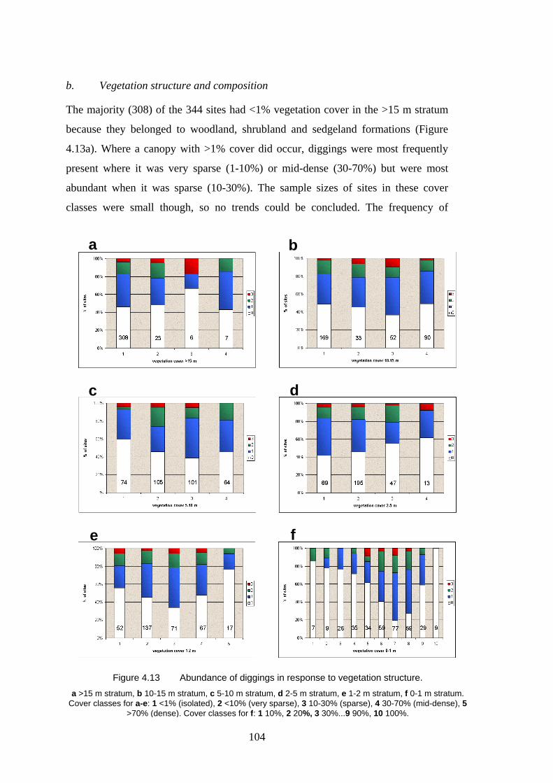
104

b. Vegetation structure and composition

The majority (308) of the 344 sites had <1% vegetation cover in the >15 m stratum

because they belonged to woodland, shrubland and sedgeland formations (Figure

4.13a). Where a canopy with >1% cover did occur, diggings were most frequently

present where it was very sparse (1-10%) or mid-dense (30-70%) but were most

abundant when it was sparse (10-30%). The sample sizes of sites in these cover

classes were small though, so no trends could be concluded. The frequency of

a b

c d

e f

Figure 4.13 Abundance of diggings in response to vegetation structure.

a >15 m stratum, b 10-15 m stratum, c 5-10 m stratum, d 2-5 m stratum, e 1-2 m stratum, f 0-1 m stratum. Cover classes for a-e: 1 <1% (isolated), 2 <10% (very sparse), 3 10-30% (sparse), 4 30-70% (mid-dense), 5

>70% (dense). Cover classes for f: 1 10%, 2 20%, 3 30%...9 90%, 10 100%.

105

diggings at sites in vegetation cover classes in the 10-15 m stratum is shown in

Figure 4.13b. The presence of diggings did not vary substantially between the four

cover classes of this stratum, with the exception of sites with 10-30% cover, which

had the highest probability of diggings being present and in high abundance. For the

5-10 m stratum, diggings were also most likely to occur at sites with 10-30% cover

(Figure 4.13c). The probability of diggings being present in the 2-5 m stratum was

greatest when the vegetation was sparse (Figure 4.13d). Sites with a cover of 30-70%

in the 2-5 m stratum had the highest probability of possessing diggings in abundance

class 3, based on a small sample of 13. In the 1-2 m stratum, sites with 10-30% cover

had the highest probability of diggings being present (Figure 4.13e). No clear pattern

of digging abundance was noticeable for this stratum with similar proportions of sites

in digging abundance classes 2 and 3 being found in each vegetation cover class,

except class 5 (>70%) which was represented by only 17 sites.

Considering that I. obesulus is a small, ground-dwelling marsupial, these

results about shrub and tree layer structure are not surprising. However, when the

distribution of diggings was compared to the structure of vegetation in the 0-1 m

stratum, a distinct pattern emerged with diggings being found most frequently at sites

with ground vegetation cover of 60-80% (Figure 4.13f). All sites in digging

abundance class 3 had 50-80% vegetation cover in this stratum. These findings are

consistent with the observations made by Paull (1993) who found that I. obesulus in

South Australia favoured sites with mid-dense to dense ground layer vegetation.

106

Figure 4.14 compares the frequency of diggings at sites with four vegetation

composition variables. Figure 4.14a shows that at 212 sites, the dominant overstorey

species was Eucalyptus baxteri. Of the remaining sites, those with E. obliqua and

shrubs as dominant species had the highest probability of diggings occurring and in

high abundance. Sites in the vegetation class other, which included Pinus radiata

mixed with species of Eucalyptus and Acacia, had a high probability of diggings

being present but not in high abundance. Ground layer species appear to relate to the

presence and abundance of diggings (Figure 4.14b). Sites had the highest probability

of diggings being present and in high abundance when Xanthorrhoea australis was

dominant in the 0-1 m stratum. Sites with ground layer vegetation dominated by

Pteridium esculentum, Leptospermum/Melaleuca or other had relatively high

probabilities of diggings occurring and in high abundance. Only one site with

diggings was found in reeds, which was in a recently dried out drainage depression.

Species richness showed a trend whereby sites with high floristic diversity had the

a b

c d

Figure 4.14 Abundance of diggings in response to vegetation composition.

a dominant overstorey species, b dominant ground layer (0-1 m) species, c number of plant species recorded at sites, d Xanthorrhoea australis height, abundance and condition score for Isoodon obesulus nests, ranging

from 1 to 6 (Appendix A4.2.2).

107

greatest likelihood of diggings being present and in high abundance (Figure 4.14c).

For the variable describing the suitability of X. australis abundance, height and

condition for nesting, sites with values of 1 and 4 had the lowest and highest

probability of diggings occurring, and the highest percentage of sites in digging

abundance class 3 occurred where the X. australis abundance, height and condition

score was 3 (Figure 4.14d).

c. Fire

Isoodon obesulus is thought to prefer vegetation in early to middle stages of

regeneration from fire but based on data collected during the field surveys, there

were no obvious relationships between the presence/absence and abundance of I.

obesulus diggings and fire. The age class of sites since last burning with the highest

probability of diggings being present was 10-14 years while sites in the two older

and younger age classes had lower probabilities (Figure 4.15a). Sites with the highest

probability of diggings occurring in abundance class 3 had not been burnt for 10-14

years. The response of diggings to the number of fires since 1957 is shown in Figure

4.15b. Sites that had been burnt 2 or 3 times had the highest probability of diggings

being present and sites burnt 5-7 times had the lowest probability. With the

exception of sites burnt twice, all classes of the variable for number of fires

contained sites with diggings in high abundance, particularly sites burnt 4 times. The

sites burnt most often, therefore, had the highest probability of diggings occurring in

high abundance but the lowest probability of diggings being present.

a b

Figure 4.15 Abundance of diggings in response to fire. a years since burning prior to 1998: 1 <5, 2 5-9, 3 10-14, 4 15-19, 5 >19 years.

b number of fires between 1957 and 1998: 1 nil, 2 1 fire, 3 2 fires, 4 3 fires, 5 4 fires, 6 5-7 fires.

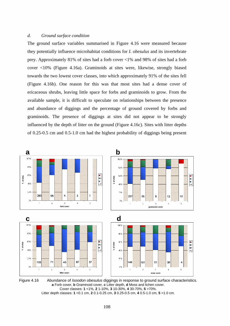
108

d. Ground surface condition

The ground surface variables summarised in Figure 4.16 were measured because

they potentially influence microhabitat conditions for I. obesulus and its invertebrate

prey. Approximately 81% of sites had a forb cover <1% and 98% of sites had a forb

cover <10% (Figure 4.16a). Graminoids at sites were, likewise, strongly biased

towards the two lowest cover classes, into which approximately 91% of the sites fell

(Figure 4.16b). One reason for this was that most sites had a dense cover of

ericaceous shrubs, leaving little space for forbs and graminoids to grow. From the

available sample, it is difficult to speculate on relationships between the presence

and abundance of diggings and the percentage of ground covered by forbs and

graminoids. The presence of diggings at sites did not appear to be strongly

influenced by the depth of litter on the ground (Figure 4.16c). Sites with litter depths

of 0.25-0.5 cm and 0.5-1.0 cm had the highest probability of diggings being present

a b

c d

Figure 4.16 Abundance of Isoodon obesulus diggings in response to ground surface characteristics.

a Forb cover, b Graminoid cover, c Litter depth, d Moss and lichen cover. Cover classes: 1 <1%, 2 1-10%, 3 10-30%, 4 30-70%, 5 >70%.

Litter depth classes: 1 <0.1 cm, 2 0.1-0.25 cm, 3 0.25-0.5 cm, 4 0.5-1.0 cm, 5 >1.0 cm.

109

and sites with <0.1 cm litter depth had the greatest likelihood of diggings occurring

in high abundance. This could have important implications for the analysis if litter in

the study area provided I. obesulus with a significant alternative foraging niche to

soil, but this is not the case because most sites in the survey had a negligible litter

cover. The presence and abundance of diggings showed little relationship to moss

and lichen cover (Figure 4.16d) but a slightly higher probability of diggings

occurring was observed for the 30-70% class.

4.3.4 Generalized Linear Modelling

What influence do the habitat variables have over I. obesulus diggings? This

question was investigated by calculating the six generalized linear models outlined in

Section 4.2.3. These models were based on two response variables: digging

presence/absence (1,0) and digging abundance classes (0: no diggings present, 1: 1-5

per 100 m, 2: 6-20 per 100 m, 3: >20 per 100 m). Models were created for three

datasets comprised of 1) 344 sites from all remnants where diggings were found, 2)

123 sites from remnants in the Mt Burr landsystem, and 3) 170 sites from remnants

in the Young landsystem. For the presence/absence models a Binomial distribution

was assumed and a Logit link function used. The Poisson distribution and Log link

function were chosen for the abundance model because abundance of diggings

classes were treated as discrete events and the number of sites in the abundance

classes had a mean and variance that were equal. Developing models for the

presence/absence and abundance of diggings allowed a comparison to be made of the

significant variables for both responses (Table 4.5)

Model 1: Presence/absence of diggings at all sites

vegetation cover in the 0-1 m stratum + Xanthorrhoea score + soil texture

On the first pass of the selection process for modelling the presence of diggings at

344 sites, 12 of the 21 variables reduced the residual deviance in the null model by a

significant (P <0.05) amount. Details are given in Appendix A10. Of these 12

variables, vegetation cover in the 0-1 m stratum accounted for the largest change in

deviance, so it was added to the model. When the Xanthorrhoea score was added to

vegetation cover in the 0-1 m stratum in the second pass, the largest change in

deviance was produced. At this stage, six other variables added to vegetation cover

110

in the 0-1 m stratum produced significant but smaller changes in deviance and they

advanced to the third pass. When soil texture was added to vegetation cover in the 0-

1 m stratum plus the Xanthorrhoea score, a significant change in deviance occurred

and it entered the model. None of the remaining variables produced a significant

change in deviance in the third pass so no further steps were taken.

When estimates for the parameters of this model are examined in Appendix

A10, it can be seen that several of the factor levels have excessively large standard

errors in relation to the estimate, particularly factor level 10 (100%) of the variable

for vegetation cover in the 0-1 m stratum. A modified model was therefore calculated

to reduce this error by combining factor levels for all three variables in the model

(Table 4.6). The modified model reduced the standard error of the parameter

estimates of the preliminary model, except the densest category of vegetation cover

in the 0-1 m stratum and it explained 117.1 of the deviance compared to 117.9 in the

unmodified version.

Table 4.5 Summary of the generalized linear models for the presence/absence and abundance of Isoodon obesulus diggings.

Significant variables were determined by forward stepwise selection. Presence/absence models assumed a Binomial distribution and used the Logit link function. Abundance models assumed a Poisson distribution and

used a Log link function. All sites n = 344, Mt Burr sites n = 123, Young sites, n = 170.

Appendix reference Fitted terms Constant +

Deviance of the null

model

Deviance explained

by the fitted terms

Model 1 - presence/absence at all sites unmodified vegetation cover in the 0-1 m stratum +

Xanthorrhoea score + soil texture 475.2 117.9

modified vegetation cover in the 0-1 m stratum* + Xanthorrhoea score* + soil texture*

475.2 117.1

Model 2 – abundance at all sites unmodified vegetation cover in the 0-1 m stratum + drainage

class + Xanthorrhoea score 367.2 97.4

modified vegetation cover in the 0-1 m stratum** + drainage class + Xanthorrhoea score*

367.2 96.7

Model 3 – presence/absence in Mt Burr unmodified vegetation cover in the 0-1 m stratum +

Xanthorrhoea score + soil texture 163.6 72.9

Model 4 – abundance in Mt Burr unmodified Xanthorrhoea score + soil texture 115.7 33.4 modified Xanthorrhoea score + soil texture* 115.6 28.9 Model 5 – presence/absence in Young unmodified dominant species in the canopy layer +

vegetation cover in the 10-15 m stratum + years since last burning + graminoid cover

234.8 70.1

Model 6 – abundance in Young unmodified dominant species in the canopy layer +

vegetation cover in the 10-15 m stratum + years since last burning

182.3 63.4

111

Model 2: Abundance of diggings at all sites

vegetation cover in the 0-1 m stratum + drainage class + Xanthorrhoea score

When modelling the abundance of diggings at 344 sites, 11 of the 21 variables

reduced the residual deviance in the null model by a significant (P <0.05) amount on

the first pass (Appendix A10). Of these, vegetation cover in the 0-1 m stratum

produced the greatest change in deviance. In the second pass, six variables produced

significant changes in the model’s residual deviance when added to vegetation cover

in the 0-1 m stratum, and the largest change was produced by adding drainage class.

Table 4.6 Factor levels for the modified generalized linear models.

Factor levels in the unmodified

models Combined factor levels in the modified models

Vegetation cover in the 0-1 m stratum

Vegetation cover in the 0-1 m stratum*

used for Model 1

Vegetation cover in the 0-1 m stratum**

used for Model 2 1 (10%) 1 1 2 (20%) 1 1 3 (30%) 1 1 4 (40%) 1 1 5 (50%) 1 2 6 (60%) 2 3 7 (70%) 3 4 8 (80%) 4 5 9 (90%) 5 6

10 (100%) 6 7 Xanthorrhoea score Xanthorrhoea score*

used for Models 1 and 2

1 1 2 2 3 3 4 4 5 5 6 5

Soil texture Soil texture* used for Models 1 and 4

C CCSL CS CCSL L CCSL

LS LS S S

Drainage class Drainage class* used for Model 2

1 1 2 1 3 2 4 3 5 4

112

In the third pass, when the Xanthorrhoea score was added to vegetation cover in the

0-1 m stratum plus drainage class, a significant change in deviance occurred. None

of the remaining variables that were carried forward from the second step produced a

significant change so no further steps were taken.

Several factor levels had large standard errors in relation to the parameter

estimates, particularly level 10 (100%) of vegetation cover in the 0-1 m stratum

(Appendix A10). A modified model was therefore calculated to reduce this error by

combining factor levels for all three variables in the model (Table 4.6). The modified

model explained 96.7 of the deviance, compared to 97.4 in the unmodified version,

leaving a residual deviance of 270.5.

Model 3: Presence/absence of diggings at Mt Burr sites

vegetation cover in the 0-1 m stratum + Xanthorrhoea score + soil texture The first two models dealt with all sites but here, a subset of 123 sites from the Mt

Burr landsystem is modelled. For the presence/absence model of diggings, 10 of the

21 variables reduced the residual deviance in the null model by a significant (P

<0.05) amount on the first pass (Appendix A10). Of these, vegetation cover in the 0-

1 m stratum was again associated with the largest change in deviance. In the second

pass, the largest change in deviance was produced when the Xanthorrhoea score was

added to vegetation cover in the 0-1 m stratum. At this stage, only one other variable

produced a significant but smaller change in the deviance when added to vegetation

cover in the 0-1 m stratum. This was soil texture and it advanced to the third pass

where it produced a significant change in deviance when added to vegetation cover

in the 0-1 m stratum plus the Xanthorrhoea score.

When estimates for the parameters were examined, many of the factor levels

had large standard errors in relation to the estimate (Appendix A10). As before, an

attempt was made to modify the model but efforts to reduce the standard error of the

estimates by combining factor levels resulted in the amount of deviance explained

falling markedly. It was decided, therefore, to make no modifications to the

presence/absence model for diggings in Mt Burr.

113

Model 4: Abundance of diggings at Mt Burr sites

Xanthorrhoea score + soil texture

On the first pass of the model for the abundance of diggings at 123 sites in the Mt

Burr Landsystem, 6 of the 21 variables reduced the residual deviance in the null

model by a significant (P <0.05) amount (Appendix A10). Of these 6 variables, the

Xanthorrhoea score was associated with the largest change in deviance. In the

second pass when soil texture was added to the Xanthorrhoea score, the largest

change in deviance was produced, so it was entered into the model. At this stage,

only one other variable produced a significant but smaller change in the deviance.

This was topographic relief class and it advanced to the third pass. When relief class

was added to the Xanthorrhoea score plus soil texture, a significant change in

deviance did not occur.

When estimates for the parameters were examined, the factor levels for soil

texture and the constant were found to have large standard errors in relation to the

estimate (Appendix A10). A modified model was therefore calculated to reduce this

error by combining factor levels for all three variables in the model as shown in

Table 4.6. The modified model explained 28.9 of the deviance, compared to 33.4 in

the unmodified version, leaving a residual deviance of 86.7.

Model 5: Presence/absence of diggings at Young sites

dominant species in the canopy layer + vegetation cover in the 10-15 m stratum + years since last burning + graminoid cover

A second subset of 170 sites from the Young landsystem was taken so that

comparisons could be made with the results from Mt Burr and all sites. On the first

pass of the model for the presence/absence of diggings in Young, 14 of the 21

variables reduced the residual deviance in the null model by a significant (P <0.05)

amount (Appendix A10). Of these 14 variables, dominant species in the canopy layer

produced the largest change in deviance. In the second pass, when vegetation cover

in the 10-15 m stratum was added to dominant species in the canopy layer the largest

change in deviance was produced. At this stage, four other variables added to

dominant species in the canopy layer produced significant but smaller changes in the

deviance. They advanced to the third pass of the model. When the variable for years

since last burning was added to dominant species in the canopy layer plus vegetation

114

cover in the 10-15 m stratum, a significant change in deviance occurred. Graminoid

cover also produced a significant but smaller change in deviance in the third pass, so

it progressed to a fourth pass where it produced a significant change in deviance

when added to dominant species in the canopy layer plus vegetation cover in the 10-

15 m stratum plus years since last burning. No variables remained and no further

passes were made.

When estimates for the parameters were examined, many of the factor levels

had large standard errors in relation to the estimate, particularly Eucalyptus ovata in

the variable for dominant species in the canopy layer (Appendix A10). Attempts to

modify the model in order to reduce the standard error of the estimates by combining

factor levels resulted in the amount of deviance explained falling markedly. It was

therefore decided to make no modifications to the model for the presence/absence of

diggings in Young.

Model 6: Abundance of diggings at Young sites

dominant species in the canopy layer + vegetation cover in the 10-15 m stratum + years since last burning On the first pass of the model for the abundance of diggings in Young, 15 of the 21

variables reduced the residual deviance in the null model by a significant (P <0.05)

amount (Appendix A10). Of these 15 variables, dominant species in the canopy layer

caused the largest change in deviance. In the second pass, when vegetation cover in

the 10-15 m stratum was added to dominant species in the canopy layer the largest

change in deviance was produced. At this stage, when the variable years since last

burning was added to dominant species in the canopy layer, a significant but smaller

change in deviance was produced. It advanced to the third pass of the model and

when added to dominant species in the canopy layer plus vegetation cover in the 10-

15 m stratum, a significant change in deviance occurred. No variables remained and

no further passes were made.

When estimates for parameters were examined, two factor levels for

dominant species in the canopy (reedland/sedgeland and Eucalyptus obliqua) had

large standard errors in relation to the estimate (Appendix A10). Attempts to reduce

these standard errors by combining factor levels reduced the deviance explained and

115

it was decided to make no modifications to the model for the abundance of diggings

in Young.

4.4 Discussion

4.4.1 Distribution and Abundance of Diggings

The results of the field survey clearly show that foraging by I. obesulus within

remnants is sporadic and approximately 47% of sites had no diggings. Where

diggings did occur, they were usually in low abundance and very few sites had

diggings in high abundance. The results confirm that I. obesulus does not occur in

large numbers in the remnants surveyed. At a regional scale, habitat for I. obesulus

has been fragmented into remnant patches through the process of land clearing but

the results of this chapter demonstrate that factors at the local scale also disrupt the

continuity of habitat for I. obesulus and thus contribute to fragmentation. These

factors include the density of ground layer vegetation (0-1 m), the abundance, height

and condition of Xanthorrhoea australis, soil texture, site drainage class, dominant

plant species in the canopy layer, vegetation cover in the 10-15 m stratum and the

number of years since last burning, which all have a different spatial ‘grain’, sensu

Wiens (1989). This conclusion has implications for conservation of the species and

this is discussed in Chapter 6. For this reason it is essential to review the sampling

methods used.

4.4.2 Sampling Methods

The method used to develop sampling units was an effective way to stratify the study

area according to topographic relief, vegetation type and fire history. Sampling of

these units in proportion to their area was generally successful, even though some

units were over sampled and others under sampled. There are numerous reasons for

this. Some of the mapped units were found not to exist in reality when field work

commenced and aberrations were caused by the combination of datasets from

different sources. Other sampling units did exist but were too small to place a single

quadrat within. Map errors, especially misclassified vegetation units, which were

corrected after field observation, complicated the process but most of the habitat

units on the base maps were sampled in proportion to their area. This resulted in the

116

collection of a large, high quality dataset that is probably one of the best of its kind at

this scale anywhere in Australia.

Using diggings to indicate the presence/absence and abundance of I. obesulus

was a successful approach because it enabled a large number of sites to be examined

in the time available for fieldwork and therefore maximised the size of the dataset.

Given more time, trapping may have been preferable for estimating the abundance of

I. obesulus at sites but as explained in Section 4.2.2b, trapping and counts of

diggings both have limitations.

Counting diggings at sites with dense vegetation in the lower stratum was

more difficult than at sites with a sparse ground layer. The counts of diggings made

during the site surveys could, therefore, be conservatively biased in areas where

there was very dense (>80% cover) ground layer vegetation. Many diggings were

found at sites where ground layer vegetation cover in the 0-1 m stratum was 60-80%

compared to sites with <60% cover, proving that I. obesulus prefers mid-dense to

sparse ground vegetation. The apparent decline in digging abundance at sites with

vegetation in the 0-1 m stratum covering >80%, as shown in the graph of Figure

4.13f, is believed to be real and not due to a threshold of visibility beyond which

diggings could not be easily observed. Indeed, it is likely that at this threshold

vegetation reaches a point where it becomes too dense for I. obesulus to move

through. It was noted during field surveys that sites with very dense (>80%) ground

vegetation often had strongly root-bound topsoil, which might be difficult for I.

obesulus to dig in. This was particularly the case at sites with dense Pteridium

esculentum where collecting soil samples with a trowel proved to be difficult due to

its roots. It has previously been concluded that sites with sparse ground layer

vegetation expose individual I. obesulus to predators while very dense vegetation

could inhibit locomotion and feeding by the species (Paull 1993, 1995). Therefore,

mid-dense ground layer vegetation can be interpreted as providing I. obesulus with

protection from predators while enabling free movement to forage.

117

4.4.3 Variables and Models

The frequency histograms in Figures 4.12-4.16 highlight 8 out of the 21 habitat

variables that relate to the presence/absence and abundance of I. obesulus diggings.

Topographic and edaphic variables consistently indicated a preference by the species

for elevated sites with good drainage, which were typical of relict sand dune

landforms. Low lying and poorly drained sites, by contrast, were not frequently or

intensively used for feeding. Vegetation cover appears to be a less important factor,

with an exception being the 0-1 m stratum. Plant communities at I. obesulus feeding

sites usually include Xanthorrhoea and a high species diversity of other flora. The

Eucalyptus woodland communities that grow on well-drained sites appear to be

preferred by I. obesulus. No clear relationships between fire and the distribution and

abundance of diggings were shown by the histograms of fire age and number of fires

(Figure 4.15) but there was some indication that recently burnt sites were avoided.

Sites of an intermediate age since last burning (10-14 years) had a slightly increased

probability of diggings occurring, as did sites that had experienced an intermediate

fire frequency of 2 to 3 fires since 1957. It is difficult to relate this finding to that of

Stoddart and Braithwaite (1979) regarding the preference of I. obesulus for

vegetation in the early stages of regeneration from fire. This is because their sample

of sites was very small, it only applied to Cranbourne near Melbourne and included a

much smaller range of vegetation types and disturbance ages than examined in the

present study.

The results for fire are potentially important for the future management of I.

obesulus habitat, which will be discussed in the next section and the next chapter but

variables relating to ground surface condition appeared to have little or no influence

over the distribution of I. obesulus diggings. These variables were not considered in

the stratification design, which may explain why many classes were under-sampled,

giving an incomplete picture about their potential influence on I. obesulus.

The distribution of diggings did not simply point to places where one

important habitat component existed, instead diggings revealed places where

interactions amongst significant variables occurred. These interactions became

apparent when generalized linear models were developed to explore relationships

118

between habitat variables and diggings. The generalized linear models highlighted

many habitat variables that produced a significant (P <0.05) change in the deviance

of the null models on the first pass but only a few made significant changes to the

residual deviance in the later stages of the stepwise process. Using all 344 records

together, the most important variables were vegetation cover in the 0-1 m stratum,

the Xanthorrhoea australis height, abundance and condition score, soil texture and

drainage class. Loamy sand and sandy soil textures increased the probability of

diggings occurring, while diggings were most abundant at sites with well-drained

soils.

When site data from the two landsystems Mt Burr and Young were modelled,

a different set of significant variables emerged and this could be due to the different

landform, soil and vegetation patterns found in each landsystem. Mt Burr is a

generally well-drained upland where Eucalyptus baxteri woodland grows on sandy

soils whereas Young is a low-lying landsystem in which a more complex mosaic of

habitats is created by woodlands on sandy dune rises and shrub, reed and sedge

communities in low, poorly drained depressions. For Mt Burr, the presence/absence

of diggings was explained by the same three variables in the presence/absence model

using all 344 sites, which were vegetation cover in the 0-1 m stratum, the

Xanthorrhoea australis height, abundance and condition score and soil texture. The

model for abundance of diggings in Mt Burr included only the latter two variables,

indicating that foraging intensity occurred irrespective of vegetation cover in the 0-1

m stratum provided that the height, abundance and condition of X. australis and soil

texture were appropriate for I. obesulus. In Young, the presence/absence and

abundance of diggings were explained by different variables to Mt Burr. The most

frequently and intensively used sites were Eucalyptus open woodlands, particularly

those dominated by E. obliqua and E. baxteri with a fire age of 10-14 years. The

variable for graminoid cover was significant in the presence/absence model for

Young, with the probability of presence of diggings decreasing as graminoid cover

increased. Very few sites were sampled where graminoids were abundant and this

variable was considered unlikely to exert much influence over the distribution of I.

obesulus.

119

4.4.4 Local Scale Fragmentation and Implications for Habitat Management

The results of this chapter indicate that muliple variables disrupt the continuity of

habitat for I. obesulus at the local scale. Recognizing these patterns will be important

for the future conservation of the species in the South East, especially when so little

habitat remains and it is fragmented at multiple scales. Local scale variations in soil,

drainage and vegetation, which have developed over thousands of years (Dodson

1975b, 1975c, 1977, Dodson and Wilson 1975), create a natural pattern of

fragmentation. In the Young landsystem fire also exerts a significant influence over

I. obesulus habitat, and this introduces a human-induced pattern of fragmentation.

The age of sites since last burning was identified by two of the generalized

linear models to be a significant variable, suggesting that controlled burning might

be a useful management tool for enhancing I. obesulus habitat and manipulating

fragmentation patterns in the Young landsystem. These statistical models are not

likely to be applicable to other places even as close as the Mt Burr landsystem

because “regression equations do not necessarily represent causal effects [so] they do

not allow extrapolation outside the range of parameter values of the specific situation

the model was tuned on” (Verboom et al. 1993 p 173). The models for all 344 sites

and for 123 sites in the Mt Burr landsystem emphasized the importance of mid-dense

ground layer vegetation, but fire reduces this stratum and it can take years to

regenerate before providing a useful structure for I. obesulus (Paull 1995). It is

therefore important that plans for burning in the remnants be guided by the following

precautionary principle. Isoodon obesulus requires dense ground layer vegetation

and if too much burning takes place then local scale fragmentation will increase with

only small portions of the remnants being suitable at any given time. Chapter 5

focuses on this local scale management issue for I. obesulus by investigating the

spatial effects produced when human-induced fragmentation by fire is superimposed

over the natural fragmentation pattern created by vegetation.

121

CHAPTER 5 LOCAL SCALE II. FIRE AND HABITAT SUITABILITY

FOR ISOODON OBESULUS

5.1 Introduction

The generalized linear models developed in Chapter 4 showed that the age of

vegetation since burning could influence the distribution of I. obesulus diggings in

native vegetation remnants in the Young landsystem. The aim of this chapter is to

examine habitat fragmentation in more detail and specifically in remnants in Young

by creating GIS habitat models under two fire management scenarios and projecting

these into the future. An alternative to the habitat suitability index approach used in

Chapters 2 and 3 is to combine GIS data using a generalized linear model, thus

making spatial predictions of the probability of a species’ occurring (Nicholls 1989).

Using maps of vegetation and fire management blocks, spatial predictions were made

of the probability of I. obesulus diggings occurring in remnants in Young when

blocks were either burnt or not burnt from 1998 to 2013.

5.1.1 Fire Management in the South East

Fire management in the South East of South Australia has evolved over a long period

of time. The death of the last full blood Bunganditj occurred in approximately 1900,

only 60 years after settlement of the region by Europeans (Pretty et al. 1983) and

very little local knowledge of Aboriginal burning practices has been preserved. The

open, grassy parkland structure encountered by explorers and early settlers of the

South East (Angas 1847) has been attributed by ForestrySA (1999) to high

frequency, low intensity burning by Aborigines. Early newspaper records reproduced

in ForestrySA (1999) indicate that, after European settlement, large bushfires became

a relatively common feature of the region in the second half of the 1800s and through

the 20th Century. The most damaging of these was the Ash Wednesday bushfire of

1983, which burnt approximately 18 000 ha of pines in the study area (Keaves and

Douglas 1983) as well as large areas of pasture and cropland and many native

vegetation remnants. Since European settlement, wildfires have caused considerable

122

loss of property and life and the modern, non-Aboriginal inhabitants have gradually

adopted their own fire strategy and burnt native vegetation as a form of risk

management. As long ago as 1917, prescribed burning by the Woods and Forests

Department (the predecessor of ForestrySA) was employed to protect pine

plantations from wildfire (Hemmings 1917 cited in ForestrySA 1999). Until

approximately 50 years ago, native vegetation was extensive but as clearance

progressed following the Second World War and, in response to bushfires in 1957

and 1958, a fire-break and track system was established around and within the

rapidly shrinking remnant patches. From then on, controlled burning of designated

fire management blocks within the remnants has been conducted under the direction

of ForestrySA and its predecessor.

The objectives of ForestrySA’s current fire policy are to burn these blocks at

varying intensities and intervals in order to:

• create and maintain floristic and structural diversity; • optimise species presence and minimise further local extinctions; • reduce wildfire intensities to improve survival and re-colonisation opportunities;

and • protect assets by fuel reduction in limited strategic areas (ForestrySA 1999).

As a requirement of the South Australian Native Vegetation Act 1991, ForestrySA

must develop management plans for the areas of native vegetation under its control

and the plans nominate blocks that will be burnt in coming years. The age of

vegetation in 1998 since last burning in Diagonal Road, Grundy Lane, Hacket,

Honan and Wandilo is shown in Figure 5.1, along with proposed burns. A total of 26

low intensity burns are planned in these remnants by 2013, comprising seven fires in

Grundy, six fires in Hacket and 13 fires in Honan, representing 67%, 77% and 67%

of the remnants’ areas respectively. No plans are in place to burn blocks in Wandilo

because the entire remnant, with the exception of approximately 20 ha, was burnt in

a wildfire in February 2000 (Figure 5.2). No plans exist to burn Diagonal Road,

which is adjacent to Honan. It is unlikely that all of the proposed fires will be lit on

schedule in the proposed years because there are many operational constraints

including weather conditions, climate and availability of personnel to perform the

burns. Nevertheless, for the purpose of modelling the burn scenario, it was assumed

that all fires would take place according to the dates shown on Figure 5.1.

123

Figure 5.1 Age of fire management blocks since last burning and dates of proposed fires.

Number of years in 1998 since blocks had burnt.

Figure 5.2 Effect of fire on Xanthorrhoea australis.

Eucalyptus baxteri and Xanthorrhoea australis before and after the Wandilo bushfire of February 2000.

124

5.2 Methods

5.2.1 Generalized Linear Model for Vegetation and Fire

A generalized linear model was created to predict the presence/absence of I. obesulus

diggings based on two mappable variables, dominant plant species in the canopy

layer and years since last burning. These two variables could be adequately

represented in the GIS unlike other variables recorded in the field and included in the

generalized linear models of Chapter 4. Many of the significant variables in Chapter

4, such as vegetation cover in the 0-1 m stratum could not be used to make spatial

predictions because they had very fine grain spatial heterogeneity that could not be

mapped over a wide extent. Dominant canopy layer species could be mapped from

air photos and field reconnaissance and this provided a useful surrogate for the

landforms, soils and drainage properties of sites. The relative relief of sites within

remnants was mapped in the GIS but this variable was shown by the generalized

linear models in Chapter 4 to have little significance, hence it was not used in this

modelling exercise.

For the map of years since last burning (Figure 5.1) the boundary of each fire

block was based on surveys conducted by ForestrySA using differential GPS and

theodolites (Des Kloeden pers. comm.). Fire records for each block were scrutinised

while compiling the fire database (Section 4.2.1c) and it was considered that there

were very few errors, if any, in the resulting fire map. Most of the fires events

mapped in the GIS were recorded as having completely burnt the blocks in which

they were lit. The fire map, therefore, offered an excellent representation of the fire

history of the remnants in the Young landsystem. It also contained ForestrySA’s

proposed burns, which provided the opportunity to model two future scenarios: one

of implementing all the proposed burns and one of conducting no burns.

The same set of data from 170 sites in Young that was used in Chapter 4 was

used again in this chapter to calculate a generalized linear model. From the statistical

model, a series of maps were then constructed to show the probability of diggings

occurring under the burn and no-burn scenarios in the blocks of Grundy, Wandilo,

Hacket, Diagonal Road and Honan.

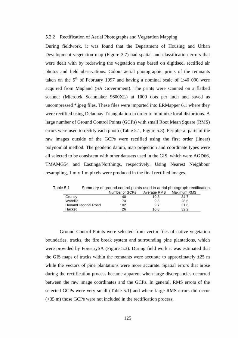
125

5.2.2 Rectification of Aerial Photographs and Vegetation Mapping

During fieldwork, it was found that the Department of Housing and Urban

Development vegetation map (Figure 3.7) had spatial and classification errors that

were dealt with by redrawing the vegetation map based on digitised, rectified air

photos and field observations. Colour aerial photographic prints of the remnants

taken on the 5th of February 1997 and having a nominal scale of 1:40 000 were

acquired from Mapland (SA Government). The prints were scanned on a flatbed

scanner (Microtek Scanmaker 9600XL) at 1000 dots per inch and saved as

uncompressed *.jpeg files. These files were imported into ERMapper 6.1 where they

were rectified using Delaunay Triangulation in order to minimize local distortions. A

large number of Ground Control Points (GCPs) with small Root Mean Square (RMS)

errors were used to rectify each photo (Table 5.1, Figure 5.3). Peripheral parts of the

raw images outside of the GCPs were rectified using the first order (linear)

polynomial method. The geodetic datum, map projection and coordinate types were

all selected to be consistent with other datasets used in the GIS, which were AGD66,

TMAMG54 and Eastings/Northings, respectively. Using Nearest Neighbour

resampling, 1 m x 1 m pixels were produced in the final rectified images.

Ground Control Points were selected from vector files of native vegetation

boundaries, tracks, the fire break system and surrounding pine plantations, which

were provided by ForestrySA (Figure 5.3). During field work it was estimated that

the GIS maps of tracks within the remnants were accurate to approximately ±25 m

while the vectors of pine plantations were more accurate. Spatial errors that arose

during the rectification process became apparent when large discrepancies occurred

between the raw image coordinates and the GCPs. In general, RMS errors of the

selected GCPs were very small (Table 5.1) and where large RMS errors did occur

(>35 m) those GCPs were not included in the rectification process.

Table 5.1 Summary of ground control points used in aerial photograph rectification. Number of GCPs Average RMS Maximum RMS Grundy 40 10.8 34.7 Wandilo 74 9.3 28.6 Honan/Diagonal Road 102 9.7 31.6 Hacket 26 10.8 32.2

126

After rectifying the raw images, polygons depicting vegetation community

boundaries were screen-digitised using ArcView. Each polygon was then assigned to

one of the seven vegetation classes used in the generalized linear models in Chapter

4, based on field survey data and interpretation of the colour, texture and pattern of

features on the photos. In addition, unpublished vegetation maps of Honan and

Grundy that were drawn during the 1960s were provided by ForestrySA. These were

referred to in conjunction with the Department of Housing and Urban Development

vegetation map when classifying dominant species on the new vegetation map.

5.2.3 Fire Scenarios and GIS Modelling

Using a generalized linear model and ArcView, the vegetation map was combined

with maps of the age of blocks since last burning to predict the probability of

diggings occurring under the two fire scenarios at three year steps from 1998 to

2013. A series of six spatial models was first created based on conducting all of the

burns shown in Figure 5.1. Using ArcView 3.2a, a grid file with a cell size of 25 m

was

#

##

#

##

#

##

#

#

##

# #

##

###

###

###

##

## ##

#

###

######

##

###

###

##

# #

#

# # #

##

##

# # ##

###

#

#

###

#

#

# #

##

#

##

# #

##

##

# #

####

#####

#

#

#

##

# #

##

#

#

#

#

#

#

#

#

####

## #

#

#

## #

##

# #####

#

## #

#

#

#

# ##

#

# ##

#

#

##

##

#

##

###

#

#

# ##

##

#

#

##

#

#

###

#

##

#

#

#

#

#

##

##

#

#

##

#

#

#

# #

#

#

##

#

###

#

#

#

#

# # #

# #

#

#

#

#

#

##

#

#

##

# #

###

#

#

#

#

#

#

#

##

##

N

0 2 km

ground control point#

native vegetation

pine plantation

Figure 5.3 Ground control points used to rectify the aerial photographs.

127

used to represent dominant canopy species and this was overlaid by grids of the age

of blocks since last burning at three year intervals. The combined vegetation/fire age

units that were produced by each overlay were reclassified using probability

estimates obtained from the generalized linear model. A second series of six spatial

predictions involving no deliberate burning was made using the same method. In

both scenarios it was assumed that no fires occurred between 2010 and 2013. The

resulting models assumed that vegetation communities did not vary their spatial

distribution throughout the entire scenario period but their age since burning did alter

with each of the time steps. In this sense, the models represented regeneration of the

pre-fire vegetation not succession where dominant plant species change over time.

5.3 Results

5.3.1 Generalized Linear Model

The generalized linear model used to estimate the probability of diggings is

summarized in Table 5.2. As with the presence/absence model for Young (Model 5

in Chapter 4), the dominant overstorey species and number of years since burning

explained 34.5 (P <0.001, 6 df) and 12.6 (P <0.05, 4 df) of the deviance,

respectively, in the first pass of the variable selection process. Dominant overstorey

species therefore entered the model and at the second pass, when number of years

since burning was added to this first variable, the residual deviance was reduced by

11.0 (P <0.05, 4 df). The parameter estimates for this model (Table 5.2b) had

relatively high standard errors, nevertheless the probability estimates shown Table

5.2c were used to create spatial models that predicted the occurrence of diggings

under different combinations of vegetation type and fire regeneration age in Grundy,

Hacket, Honan, Diagonal Road and Wandilo under the burn and no-burn scenarios.

128

Table 5.2 Generalized linear model for sites in Young using vegetation and fire to

predict Isoodon obesulus diggings.

a) Change in deviance analysis. deviance [change in deviance(degrees of freedom)] *<0.05, **<0.01, ***<0.001

1st pass

2nd pass Assoc + [34.5]

Null model 234.8

ASSOC 34.5 (6)*** - F_AGE 12.6 (4)* 45.5 [11.0(4)*]

b) Estimate of parameters. Fitted terms: Constant + ASSOC + F_AGE

Factor reference levels: Assoc (eucbax); F_age (0-4 years)

Estimate s.e. Constant -0.789 0.381 ASSOC eucobl 0.120 1.030 ASSOC eucova -0.724 0.394 ASSOC eucvim -0.548 0.610 ASSOC other 0.136 0.326 ASSOC reed/sedge -2.868 0.998 ASSOC shrubs -0.554 0.311 F_AGE 2 (5-9 years) 0.972 0.418 F_AGE 3 (10-14 years) 1.141 0.419 F_AGE 4 (15-19 years) 0.518 0.424 F_AGE 5 (>19 years) 0.668 0.432

c) Probability estimates and (standard errors) for diggings in vegetation associations of different ages since last burning.

0-4 years 5-9 years 10-14 years 15-19 years >19 years eucbax 0.46 (0.13) 0.80 (0.07) 0.83 (0.07) 0.57 (0.08) 0.63 (0.10) eucobl 0.99 (0.09) 1.00 (0.02) 1.00 (0.02) 0.99 (0.06) 0.99 (0.04) eucova 0.16 (0.10) 0.46 (0.17) 0.51 (0.17) 0.23 (0.11) 0.27 (0.14) eucvim 0.34 (0.23) 0.71 (0.20) 0.75 (0.19) 0.45 (0.23) 0.51 (0.21) other 0.54 (0.22) 0.84 (0.11) 0.87 (0.10) 0.65 (0.19) 0.70 (0.15) reed/sedge 0.02 (0.03) 0.10 (0.10) 0.12 (0.12) 0.04 (0.04) 0.05 (0.05) shrubs 0.26 (0.12) 0.62 (0.14) 0.66 (0.14) 0.35 (0.12) 0.41 (0.13)

129

5.3.2 Rectified Aerial Photographs and Vegetation Maps

The rectified air photos with screen-digitised polygons of vegetation community

boundaries are shown in Figure 5.4. The combination of remote sensing

interpretation, existing vegetation maps and observations made at 142 sites in these

remnants during the field surveys resulted in greatly improved vegetation mapping,

which was classified according to the same seven communities entered into the

generalized linear models in Chapter 4 (Figure 5.5). Eucalyptus baxteri occupied the

greatest total area but notable areas of E. ovata were mapped in Grundy and

Wandilo. Smaller areas of reed/sedge and shrubs were interspersed with E. baxteri

and E. ovata woodlands in each of the remnants. Eucalyptus obliqua was mapped in

only one area, which was in Honan. The absolute and relative total areas of the seven

vegetation classes were: E. baxteri 1967.5 ha (61.8%), reed/sedge 402.3 ha (12.6%),

shrubs 338.1 ha (10.6%), E. ovata 199 ha (6.3%), other 199.8 ha (6.3%), E. viminalis

69.3 ha (2.2%) and E. obliqua 6.4 ha (0.2%).

Figure 5.4 Rectified aerial photographs of remnants in the Young landsystem. Vegetation boundaries are shown by screen-digitised polygons over the aerial photographs.

130

5.3.3 Spatial Predictions under the Burn and No-Burn Scenarios

The predicted probability of diggings occurring under the burn scenario is shown at

three year intervals in Figure 5.6. When the predictions for 1998 and 2013 are

compared it appears that habitat would be enhanced by conducting the proposed

burns. The time series in three year increments, however, suggests the probability of

diggings occurring declines in some parts of the remnants before recovering by 2013.

Under the burn scenario, Grundy is predicted to have a greatly reduced area with

high probability of diggings occurring between the years 2004 and 2010, and this is

shown by the temporally continuous annual data in Figure 5.8. It appears that

conducting all of the proposed burns in this remnant could potentially reduce the

availability of habitat and accentuate fragmentation to a point where I. obesulus

becomes locally extinct from Grundy. Alternatively, not conducting the planned

burns in Grundy would reduce the probability of diggings being present throughout

the remnant by 2013 (Figure 5.7). An obvious conclusion from this analysis is that

the burning proposals for Grundy need to be reviewed.

Figure 5.5 Vegetation classification of remnants in the Young landsystem.

Based on interpretation of aerial photographs, previous vegetation mapping and field validation.

eucbax Eucalyptus baxteri, eucobl E. obliqua, euco va E. ovata, eucvim E. viminalis, other Acacia spp. and Pinus radiata mixed with Eucalypts, reed/sedge Phragmites australis, Typha domingensis, Gahnia spp.,

Isolepis nodosa, Lepidosperma spp. shrubs Leptospermum continentale, Melaleuca squarrosa, M. brevifolia

131

The model for the Wandilo blocks with no burning indicates that there will be

a low probability of diggings being found throughout the remnant until

approximately 2007. This also assumes that individual I. obesulus survived the

wildfire of February 2000 or that Wandilo will be recolonised from surrounding

remnants before 2007. By 2010, as vegetation matures, approximately 60% of

Wandilo could have a probability >80% of diggings occurring (Figure 5.8).

Considering that the time required for all vegetation classes to reach their maximum

probability of diggings being present is 10 to 14 years, there would be no imperative

to burn blocks within Wandilo during the planning period, although there may be

some justification to do so around or soon after 2010-2013.

Like Wandilo, no fires are planned for Diagonal Road and because all parts

of this remnant were burnt >19 years before 1998, no change is seen in any of the

models throughout the scenario period to 2013. Fire therefore plays no role in the

spatial distribution of diggings in the Diagonal Road predictions, and the fragmented

habitat patterns seen in Figures 5.6 and 5.7 are due to vegetation alone.

In Honan, the proposed burning program is predicted to increase the

probability of I. obesulus occurring throughout much of the remnant by 2013

compared to the scenario of no fires that would see a reduction in the probability of

diggings occurring. In this relatively large remnant with many blocks, the use of fire

is therefore likely to reduce fragmentation and this can be seen in Figure 5.6. For the

period 2001 to 2007, it was predicted that slightly larger areas of Honan would have

an increased probability of diggings occurring if no burning took place than if the

fires were lit. Subsequent to 2007, however, the reverse is likely to occur because the

scenario for no controlled burns would lead to a significant reduction in the area of

habitat with a high probability of possessing I. obesulus diggings. In Hacket, the

spatial models predicted that the probability of diggings would decline if burning

was not conducted but if the fires were lit then a considerable increase would occur

in the area of Hacket with a high probability of diggings towards 2013. As with

Honan, the plan to use fire in Hacket is likely to reduce fragmentation and increase

the area of high quality habitat.

132

These results point to a very complex response conditional upon only two

variables, dominant species in the canopy layer and years since burning. As

demonstrated in Chapter 4, at least four other variables influence the presence or

absence of I. obesulus diggings because when sites from all landsystems were

analysed, vegetation cover in the 0-1 m stratum, the Xanthorrhoea australis score,

drainage class and soil texture were found to be significant. When 170 sites from

Young were analysed, vegetation cover in the 10-15 m stratum was significant in

combination with years since burning and dominant species in the canopy layer. The

former and latter of these three variables are likely to be strongly associated and

using just two explanatory variables in the generalized linear model in this chapter

assisted the interpretation of the spatial models.

133

2001

2004 2007

2010 2013

1998

Figure 5.6 Probability of diggings occurring under the burn scenario.

Probability of diggings occurring under the scenario that all proposed burns are conducted between 1998 and 2013.

134

2001

2004 2007

2010 2013

1998

Figure 5.7 Probability of diggings occurring under the no-burn scenario. Probability of diggings occurring under the scenario that no fires are lit between 1998 and 2013.

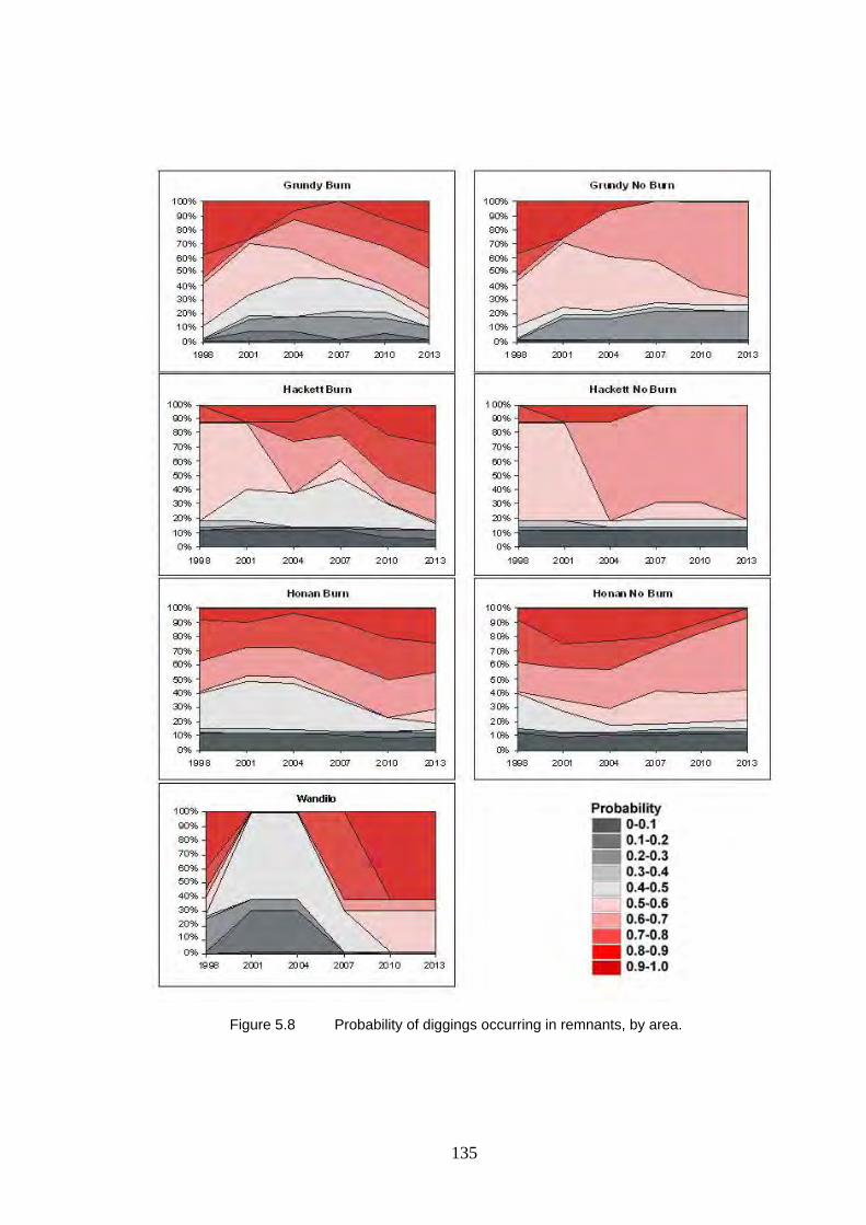
135

Figure 5.8 Probability of diggings occurring in remnants, by area.

136

5.4 Discussion The spatial models presented in this chapter could not be validated in the field

because, apart from 2001, the time intervals have not yet occurred. Additionally,

because the standard errors associated with the probability estimates were large, it

was considered unnecessary to visit sites predicted by the model. The ecological

model presented in this chapter should therefore be considered ‘strategic’ rather than

‘tactical’ (May 1973, Gilman and Hails 1997) and should not be used for planning

particular burns. The model is simplistic because it assumes all fires have a uniform

effect and ignores the fact that they burn with differing intensities. In addition,

important variables identified in Chapter 4 were not included in the spatial

predictions due to the difficulty of mapping them at this scale. Other potentially

important factors not examined in Chapter 4, such as the distribution of predators and

subterranean invertebrate food for I. obesulus, were also ignored.

Although the predictive power of the models is not great, the approach is

useful because it highlights spatial relationships between vegetation and the principal

habitat management tool used in the study area, which is fire. Using this approach,

areas were identified where existing fire plans could be modified to the advantage of

I. obesulus. Grundy is a small remnant that may be burnt too much under the current

proposals. Carrying out the burning scenario could limit the amount of high quality

habitat available in Grundy for several years and greatly increase fragmentation,

which may in turn lead to the local extinction of I. obesulus from the remnant.

Paradoxically, the model suggested that not burning Grundy would also lead to a

gradual decline in the probability of diggings occurring as vegetation matures. This

is also the case for other remnants under consideration, the exceptions being Wandilo

due to its recovery from the February 2000 wildfire and Diagonal Road, which has

not been burnt for many years. For Honan and Hacket, the models suggest an

increase in habitat quality and a decrease in fragmentation if the burns go ahead. To

interpret these models it is important to understand the history of fire within the

remnants, not just proposals to burn in the future.

Besides the limitations of the model that arise from its simple nature, it is

strongly emphasized that the model is specific to the Young landsystem and its

application in other places would be problematic. In Chapter 4, it was shown that the

137

abundance of diggings in the Mt Burr landsystem is not related to the age of sites

since last burning. With regard to previous observations about I. obesulus and fire,

for example those by Stoddart and Braithwaite (1979), the conclusion of the present

study is that the fire regeneration age of sites may relate to the quality of habitat in

some of the landsystems occupied by the species but not all.

This is not the first time that an assessment of burning strategies in the South

East has been made. Possingham and Gepp (1993, 1996) used Population Viability

Analysis (PVA) to assess fire management options for I. obesulus in Honan. Central

to their model was an assumption that habitat suitability is zero in the first year after

a burn; it increases to maximum suitability after 5 years, stays at this level for

another two years and then slowly declines to 25% of the maximum after 25 years.

They concluded that to minimise the likelihood of extinction of I. obesulus from

Honan, the optimal interval between fires was 18 years for blocks. This interval is

slightly longer but consistent with the probability estimates calculated in the present

study and shown in Table 5.2c. Possingham and Gepp (1993, 1996) considered their

results to be counter-intuitive because the function they adopted for habitat quality

and the burn interval for minimizing extinction risk were out of phase by

approximately ten years. They conducted sensitivity analysis by modifying the

habitat quality function and produced further results that indicated burning earlier or

later than 18 years could be advantageous but never before ten years from a previous

burn.

Understanding the underlying pattern of habitat suitability will be necessary

for defining effective management zones within the remnants. Fire planning needs to

consider the variables that fragment the distribution of I. obesulus at the local scale

because existing fire blocks may be placed inappropriately compared to the

ecological zones of the remnants. Some adjustment to the spatial pattern of burning

could therefore be necessary. A solution may be to burn smaller compartments

because some remnants have been divided into very few management blocks

compared to their total area and almost any fire within the remnants will burn a large

percentage of the available habitat. Lighting small fires might not be feasible for

operational reasons and there is a danger of increasing habitat fragmention by

creating new tracks around additional management blocks, which has a great

138

potential to facilitate predator infiltration (May and Norton 1996). Another issue is

that past fires have burnt to the edges of blocks but not beyond, so complex ecotonal

patterns are not created by overlapping fire scars. The current fire perimeter system

is rigid but perhaps subsections of existing blocks could be burnt at a higher or lower

frequency and be allowed to overlap into subsections of adjacent fire blocks. This is

all dependent on the ability of fire managers to control the burns.

Reinstatement of Aboriginal burning practices is impossible because little is

known about traditional methods in the South East and the landscape structure has

changed. Likewise, early European burning practices in the study area have little

relevance in modern times because most of the native vegetation has been cleared. If

the results of this study are to provide any guidance, then fires should not be lit

frequently in areas identified as having high habitat suitability for bandicoots based

on other significant variables such as soil, drainage and vegetation cover. Perhaps a

15 to 20 year minimum period between fires could be planned for such important

areas and, even then, patchy burning should be conducted at a low intensity. Fires in

the South East are usually lit in spring, which coincides undesirably with the

breeding of I. obesulus but there is probably not much scope to vary the season

unless autumn burns are considered.

139

CHAPTER 6

CONCLUSION

6.1 Major Findings of the Study

This thesis has examined the distribution of Isoodon obesulus at multiple spatial

scales. Each of these scales revealed a fragmented habitat or, according to the

definition of Lord and Norton (1990 p 197), a “disruption of continuity”. Conducting

the study at multiple scales required the use of a range of methodologies and also

required changes in methods with the different scales. At the continental and regional

scales, archived records, bioclimatic models and broad scale thematic maps of

geology, soils and vegetation were used but at the local scale it was necessary to

collect detailed field data in order to assess habitat fragmentation.

There is little doubt that habitat fragmentation caused by natural and human-

induced phenomena occurs at multiple spatial scales (Figure 6.1). At the continental

Continental scale(subspecies)

Continental scale(species)

Regional scale

Local scale

Figure 6.1 Fragmentation of Isoodon obesulus habitat at multiple spatial and temporal scales.

140

scale, habitat suitability maps indicated that climate, geology and vegetation

fragmented the distribution of I. obesulus. These maps were based on BIOCLIM and

BIOMAP analyses of archived records of I. obesulus and they were combined with

weighted suitability maps of geology and vegetation using ArcView GIS. The

geology and vegetation layers were combined in equal weight with the BIOMAP

output to predict the distribution of habitat suitability for I. obesulus in 1788 and

1988.

The output of the BIOCLIM and BIOMAP analyses provided a prediction of

the distribution of I. obesulus that closely matched its known distribution. High

geologic and vegetation suitability indices were predicted for a much larger area than

climate, however, when the addition of geology and vegetation was made to climate

suitability, the maps more closely resembled the species’ known distribution. The

variables of climate, landforms and vegetation are interdependent and it was assumed

that combinations of these factors determine the continental scale distribution of I.

obesulus habitat.

A significant finding was that the fragmented continental distribution of the

subspecies almost certainly existed prior to European settlement because of

biogeographic isolating mechanisms in the form of climate, geologic and vegetation

barriers. The implication of this finding is that regional populations of I. obesulus

have probably been fragmented from one another long enough to influence their

evolutionary development.

The regional scale GIS predictions of habitat suitability presented in Chapter

3 provided information that was not revealed by the continental scale analysis of

Chapter 2. By combining the continental scale prediction of climate suitability with

higher resolution mapping of soil types and floristic associations, a prediction was

made of the pre-European and current distribution of I. obesulus in the South East of

South Australia. This region is typical of the regions in which I. obesulus occurs

because it has been extensively cleared and replanted with introduced species. As

with the continental scale analysis of Chapter 2, this regional scale land cover

transformation has forced a new pattern of habitat fragmentation over the pre-

European distribution of I. obesulus, which was fragmented by soil and vegetation

141

variations according to the model presented in Chapter 3. The naturally fragmented

distribution of I. obesulus habitat in the South East has therefore had the effects of

European settlement imprinted over it, and native vegetation has been converted into

exotic land cover types including pasture, cropland and pine plantations.

By analysing land cover change in the South East, it was found that

conversion from native vegetation to pine plantation caused a greater decline in

habitat suitability for I. obesulus than conversion to cropland and pasture, even

though the latter is now far more extensively distributed. This is because the pine

plantations have been placed where soil and climate are most suitable for I. obesulus.

Identifying areas where soil and climate are suitable for I. obesulus and which could

potentially be revegetated, may be important for the future expansion of its highly

reduced and fragmented habitat in the South East.

When assessing the fragmented distribution of I. obesulus at the third and

finest scale, which is the local scale within remnants of native vegetation, the

stratified sampling methodology using GIS presented in Chapter 4 enabled different

habitat types to be surveyed in the field in proportion to their area. This sampling

approach ensured that the input data for statistical analyses were representative of the

range of habitat types available to I. obesulus. Statistical analyses of the field survey

data using generalized linear models revealed a range of factors likely to influence

the local scale distribution of I. obesulus.

A total of 372 sites was surveyed in 29 remnant patches and for the statistical

analysis 344 sites from 25 remnant patches were used. This large data set was

analysed first in its entirety and then partitioned in order to model the distribution of

the subspecies in two adjacent landsystems, Mt Burr which is a well-drained upland

and Young which is a low lying and generally poorly drained landsystem. By

building generalized linear models for all 344 sites then partitioning the data for the

two landsystems, different variables were found to influence the distribution of I.

obesulus.

The generalized linear models revealed the variables that exerted the greatest

influence over the presence/absence and abundance of I. obesulus diggings. The

significant variables in the models showed a consistent pattern, regardless of whether

142

presence/absence or abundance of diggings was modelled. For example, vegetation

cover in the 0-1 m stratum, the abundance of Xanthorrhoea and soil texture were

emphasized in both the presence/absence and abundance models for all sites and for

Mt Burr sites. By contrast, dominant overstorey species, vegetation cover in the 10-

15 m stratum and years since burning were the variables emphasized in both the

presence/absence and abundance models for Young. Based on the findings at two

sites in Victoria, Stoddart and Braithwaite (1979) concluded that time since burning

may influence habitat selection by I. obesulus but, based on a much larger number of

sites, the present study concluded that other factors including vegetation and soil

were more important. Fire was found to be a significant factor only in the Young

landsystem and it was modelled with the dominant species in the canopy layer and

vegetation cover in the 10-15 m stratum.

The results of Chapter 4 indicated a general pattern of habitat selection by I.

obesulus at the local scale where its diggings are most frequently present and in high

abundance on elevated sandy areas such as relict dunes. These deep, infertile sands

and podzols typically support Eucalyptus baxteri woodlands with low shrub or heath

layers. The infertile acidic sands where E. baxteri grows are sufficiently deep to

prevent its roots from reaching the limestone substrate. Areas where this community

exists are relatively well drained, even during times of flooding.

The local scale variables that were analysed were easily observed in the field

(for example vegetation structure) or extracted from the fire history database, unlike

other variables that would potentially influence the distribution of I. obesulus, such

as invertebrate food distribution and predators. In terms of practical conservation

work, use of easily observed local scale variables should greatly assist land managers

to identify suitable habitats for I. obesulus. Rapid site assessments of key habitat

variables for I. obesulus will be important in future conservation work at a local

scale, particularly with regard to planning prescribed burning.

The response of I. obesulus to fire modelled in Chapter 5, offers a possible

method for enhancing habitats through prescribed burning. The probability of I.

obesulus diggings being present within five native vegetation remnants in the Young

landsystem was mapped by combining vegetation and fire maps in a GIS using a

generalized linear model. Although other additional variables were found to be

143

significant in Chapter 4, vegetation association and fire age could be adequately

mapped in the GIS and manipulated temporally, unlike landform and soil variables

which alter over much longer time scales.

The statistical fire model enabled an evaluation to be made of the effects of

ForestrySA’s burning of I. obesulus habitat. The model is specific to the Young

landsystem and there is no suggestion that it could be applied to other landsystems.

Within Young, it functions as a strategic model because of the low number of

explanatory variables and the high error terms. Nevertheless, the model indicated

that the proposed burns could reduce fragmentation and lead to an increase in the

likelihood of I. obesulus occurring within some of the remnants burnt. The models

also identified instances where the existing fire plans should be modified because in

their current form they threaten to increase fragmentation and reduce the availability

of high quality habitat for I. obesulus. The land transformation processes of

perforation, dissection, shrinkage and attrition (Figure 1.1) are also evident in these

local scale models but not discussed in this thesis.

6.2 Conserving Isoodon obesulus at Multiple Scales

The subspecies I. o. obesulus has been listed as Endangered under the Australian

Environmental Protection and Biodiversity Act 1999 because of a severe reduction in

numbers. It also qualifies to be listed as Vulnerable under the same Act because its

geographic distribution is restricted and precarious for its survival

(http://www.deh.gov.au/biodiversity/threatened/species/bandicoot.html). At a

continental scale, the distribution of I. obesulus has become fragmented over

thousands of years by climate change and associated vegetation change. The future

of the species is now insecure partly because extensive vegetation clearance last

century stamped human-induced fragmentation over natural fragmentation, and this

is clearly visible at multiple scales of observation.

At a regional scale, the prognosis for I. obesulus in the South East of South

Australia is poor and unless steps are taken to enhance its habitat, the species may

soon become regionally extinct. The population is currently known to exist in 23

remnant patches but they are small and a single disturbance event like the Ash

Wednesday bushfires of 1983 could simultaneously affect many remnants. At a local

http://www.deh.gov.au/biodiversity/threatened/species/bandicoot.html

144

scale, I. obesulus may have become extinct in four remnants of the South East since

1990 (Brooksby, Burr Slopes, Paltridges and Mt Lyon) because no diggings were

found there during the surveys of 1998 and 1999. The matrix of pines which

surrounds native vegetation remnants exacerbates isolation for bandicoots because

there is sparse vegetation cover under the pines and no place to shelter from

predators. There is no proof that I. obesulus disperses between remnants in the South

East and it is assumed that the probability of recolonisation following local

extinction is low. It is likely, however, that further local extinctions of I. obesulus

from remnants will occur, particularly Kays, Mt McIntyre and Honeysuckle, which

were found to have very few diggings.

While the South East of South Australia can be compared with other regions

occupied by I. obesulus, it has its own unique character and conservation issues. The

general conclusion here is that every geographic region has unique characteristics

and conservation considerations. Different management regimes prevail and different

threatening processes operate, although there are common themes such as foxes, fire

and vegetation clearance. There is considerable scope at this scale for conservation

planning for I. obesulus. For example, it will be important to establish and maintain

dispersal corridors between remnant patches (Horn 2003). Some areas, such as

roadside vegetation and the edges of pine blocks, may already provide cover for

bandicoot movements and some small remnants may be used as ‘stepping stones’. To

improve connectivity between remnants, it will be important to identify and conserve

these landscape elements for dispersing bandicoots. Suitable, isolated remnants

devoid of bandicoots may also be considered for reintroductions, which are discussed

below.

The regional population appears to be declining and landscape-scale effects

arising from the area, isolation and shape of remnant patches may affect the

distribution of I. obesulus in the South East. This, however, was not the focus of the

present study, which was to investigate habitat fragmentation at the continental,

regional and local scales. While it is possible that metapopulation dynamics operate

to decrease the probability of permanent local extinction of I. obesulus in the South

East (Possingham and Gepp 1996), it is unlikely given the large inter-patch distances

in the current highly fragmented landscape configuration. Remnant patches of native

145

vegetation are obviously critical areas for I. obesulus in the South East and this is

supported by unpublished radio tracking data for the species collected by the author

in Wandilo Native Forest Reserve in 1998. It was found that 15 year old pines

abutting Wandilo were very rarely entered by bandicoots, which always stayed in

close proximity to the dense ground cover of native vegetation.

Some dispersal by I. obesulus may occur between remnants in the region and

this is high priority for suture studies. Paull (1999) speculated that three or more

metapopulations may exist, comprised of individuals inhabiting remnants in the

Nangwarry landsystem (The Heath, Byrnes and Paltridges), Caroline landsystem

(Wild Dog and Honeysuckle) and Mt Burr/Young landsystems (Figure 4.3, native

vegetation remnants surveyed). Each of these clusters of remnants is separated from

the others by wide expanses of cleared land, which would severely restrict dispersal

opportunities for I. obesulus. Extensive fieldwork focussed on reproduction,

dispersal and recruitment by the species would be necessary to investigate population

distribution at this spatial scale, and beyond the scope of the present study. Besides,

it was concluded in Chapter 3 that the combination of variables used to create Figure

3.12b, which included climate, soils and vegetation, produced a good prediction of

the known regional distribution of I. obesulus without incorporating landscape-scale

factors such as the area and isolation of remnants.

To reverse the trend of local extinction, translocating bandicoots between

neighbouring remnants may be an effective option and cheaper in the the short term

than planting vegetation corridors. If individuals for translocation were selected from

the nearest remnant, then this would closely simulate natural recolonization.

Translocating stock from further away may be problematic because important

genetic differences between I. obesulus in remnants of the South East have been

detected (Johnston et al. 1999, 2000, 2002). It would not, therefore, be appropriate to

mix individuals from the Mt Burr/Young, Caroline or Nangwarry landsystems

without first undertaking a detailed genetic survey of I. obesulus in the South East.

This is particularly the case because the regional scale prediction of pre-European

habitat suitability showed these areas to be fragmented from each other by long-

standing soil and vegetation patterns, which are likely to have led to genetic

146

divergence. Evidence to support this comes from Cooper (1998, 2000) who found

that significant morphological and genetic differences in I. obesulus exist over small

geographic distances in Western Australia. A captive population of I. obesulus

individuals sourced from the South East could act as a useful emergency reservoir if

numbers in the wild became critically low. It could also play an important role in

public education about the species. In the longer term, establishment of a corridor

network would be preferable to and cheaper than translocations or captive breeding

(Horn 2003).

6.3 Significance of the Study

This thesis will mean different things to different people. For land managers,

important data are now available on the distribution of I. obesulus and its habitats at

scales that can be compared to existing management units, such as fire blocks. The

study is also important for conservation biologists because it illustrates the spatial

structure of fragmented habitats at multiple spatial and temporal scales.

The importance of different variables changes at each scale and between

places. For example, not all regions are alike and there is no certainty that the results

obtained from the South East can be generalised to other regions. This complicates

habitat mapping and it has implications for conservation planning. Lessons learnt

from the South East that could be useful to conservation managers may be directly

applicable in other regions. What would the results be if the study had focussed on

another region inhabited by I. obesulus, such as the Mount Lofty Ranges?

Observations by the author suggest that topography might play a more significant

role in the Mount Lofty Ranges than the South East because the distribution of I.

obesulus there is associated with alluvium in valleys.

The thesis demonstrates that multiple spatial and temporal scales must be

considered when analysing habitat fragmentation. The “disruption of continuity”

(Lord and Norton 1990 p 197) can happen over continental scales by natural and

slow acting process such as climate change. Even at this scale, the effects of human-

induced fragmentation by vegetation clearance can be observed. At a finer, regional

scale, soil patterns and landform systems that have developed over thousands of

years can cause natural habitat fragmentation. During the last century, vegetation

147

clearance has superimposed a pattern of human-induced fragmentation over natural

fragmentation patterns. At the local scale, burning of management blocks within

some remnants could increase fragmentation by imprinting human-induced

disturbance over natural habitat heterogeneity but in other remnants the judicious use

of fire may over time reduce fragmentation as vegetation regenerates.

6.4 Future Research

Fragmentation of the distribution of I. obesulus was investigated in this thesis at

three spatial scales but further investigations could be undertaken at other scales, for

example the fine-scale relationships that exist between the distribution of I. obesulus

and its subterranean food supply. Braithwaite and Gullen (1978) observed that until

further knowledge of the specific plant-invertebrate relationships that regulate

bandicoot diet is acquired, the distribution of I. obesulus at a fine scale will remain a

puzzle. Another fragmentation study that could occur at a slightly coarser scale is the

influence of vehicle tracks and fire breaks on the movements of bandicoots and their

predators. At an even coarser scale, the potential for bandicoots to disperse between

remnants requires further research, probably using radiotelemetry.

It should be possible to produce similar GIS predictions of habitat suitability

for each of the regions occupied by I. obesulus but this would be dependent on the

availability of mapping. Inconsistencies in map layers and classification systems,

between regions and State mapping authorities, would necessitate unique modelling

schemes to be developed for each region. Not only would GIS data vary between

States and regions, the habitat relationships of I. obesulus to soil and vegetation

would vary, thus presenting numerous future research challenges.

The findings of this study will be important for future taxonomic research and

may aid in the interpretation of genetic relationships between I. obesulus occupying

different geographic locations. Studying genetic variation is important because

translocations of individuals within and between regions may one day be considered

as a conservation measure. Translocations of Mount Lofty Ranges I. obesulus to the

Otway/Geelong region have, in fact, recently occurred but the animals are in

captivity (Anon 2002). The species has a great capacity for escaping from fenced

nature reserves, especially when young (personal observation), and there is a local

148

and genetically distinct population in the Otway/Geelong region with which the

Mount Lofty Ranges stock can now potentially communicate. Isoodon obesulus has

therefore crossed the biogeographic barrier at the Murray River and Coorong in

South Australia, which has almost certainly been a major and long-standing genetic

division for the species (Close et al. 1990, Adams in Maxwell et al. 1996). For

planning reintroductions it is important to recognize the way genetic diversity is

spatially distributed and therefore carefully consider where to source appropriate

individuals from.

Possingham and Gepp (1993, 1996) conducted population viability analysis

(PVA) on the Honan I. obesulus population in an attempt to assess prescribed

burning schedules. The parameterization of this population model was based on

existing and very limited data for demography, fecundity and mortality, to which the

present study can not contribute. The present study can, however, make a significant

contribution to the development of future ecological models by providing a realistic

spatial framework for habitat that incorporates underlying natural fragmentation with

superimposed human-induced habitat fragmentation. In conclusion, future studies of

habitat fragmentation should consider the multiple scales at which it occurs. This

study has provided insights into the process of habitat fragmentation, which

influences the distribution and evolutionary development of species at multiple

scales and at the same time threatens their survival.

149

REFERENCES

Aitken, P. (1983). Mammals. In Natural History of the South East. (Eds M. J. Tyler, C. R. Twidale, J. K. Ling and J. W. Holmes.) pp. 127-133. (Royal Society of South Australia: Adelaide).

Allison, G. B. and Harvey, P. D. (1983). Freshwater Lakes. In Natural History of the South East. (Eds M. J. Tyler, C. R. Twidale, J. K. Ling and J. W. Holmes.) pp. 61-74. (Royal Society of South Australia: Adelaide).

Angas, G. F. (1847). Savage Life and Scenes in New Zealand and Australia: Being an Artist’s Impressions of Countries and People at the Antipodes. Smith Elder and Co. London. Reproduced by the Libraries Board of South Australia from a copy held in the State Library of South Australia, Adelaide 1969.

Anon (2002). Rare species for Victoria. The Advertiser Saturday March 9, 2002, p. 21.

Ashby, E., Lunney, D., Robertshaw, J. and Harden, R. (1990). Status of bandicoots in New South Wales. In Bandicoots and Bilbies. (Eds J. H. Seebeck, P. R. Brown, R. L. Wallis and C. M. Kemper.) pp. 43-50. (Surrey Beatty and Sons: Sydney).

Atkins, K. L. B. (1998). Habitat preference and distribution of Perameles nasuta and Isoodon obesulus in bushland remnants in Sydney. MSc Thesis, Macquarie University.

Bender, L. C., Rolof, G. J. and Haufler, J. B. (1996). Evaluating confidence intervals for habitat suitability models. Wildlife Society Bulletin 24, 347-352.

Bissonette, J. A. (1997). Scale-sensitive ecological properties: historical context, current meaning. In Wildlife and Landscape Ecology: Effects of Pattern and Scale. (Ed. J. A. Bissonette.) pp. 3-31. (Springer-Verlag: New York).

Bissonette, J. A., Harrison, D. J., Hargis, C. D. and Chapin, T. G. (1997). The influence of spatial scale and scale-sensitive properties in habitat selection by American Marten. In Wildlife and Landscape Ecology: Effects of Pattern and Scale. (Ed. J. A. Bissonette.) pp. 368-385. (Springer-Verlag: New York).

Blackburn, G. (1959). Soils of County Grey, South Australia. CSIRO Division of Soils and Land Use Series No. 33.

Blackburn, G. (1983). Soils. In Natural History of the South East. (Eds M. J. Tyler, C. R. Twidale, J. K. Ling and J. W. Holmes.) pp. 39-48. (Royal Society of South Australia: Adelaide).

Bleich, V. C., Wehausen, J. D. and Holl, S. A. (1990). Desert-dwelling mountain sheep: conservation implications of a naturally fragmented distribution. Conservation Biology 4, 383-390.

Boyce, M. S. and McDonald, L. L. (1999). Relating populations to habitats using resource selection functions. Trends in Ecology and Evolution 14, 268-272.

150

Braithwaite, R. W. (1983). Southern brown bandicoot. In The Australian Museum Complete Book of Mammals. (Ed. R. Strahan.) pp. 94-95. (Angus and Robertson Publishers: Sydney).

Braithwaite, R. W. and Gullen, P. K. (1978). Habitat selection by small mammals in a Victorian heathland. Australian Journal of Ecology 3, 109-127.

Brereton, R., Bennett, S. and Mansergh, I. (1995). Enhanced greenhouse climate change and its potential effect on selected fauna of south-eastern Australia: a trend analysis. Biological Conservation 72, 339-354.

Brooks, R. P. (1997). Improving habitat suitability index models. Wildlife Society Bulletin 25, 163-167.

Broome, L. S. and Mansergh, I. M. (1989). The mountain pygmy possum Burramys parvus (Broom): an alpine endemic. In The Scientific Significance of the Australian Alps. (Ed. R. Good.) pp. 241-264. (The Australian Alps National Parks Liaison Committee in association with the Australian Academy of Science: Canberra).

Cale, P. and Hobbs, R. J. (1994). Landscape heterogeneity indices: problems of scale and applicability, with particular reference to animal habitat destruction. Pacific Conservation Biology 1, 183-193.

Carruthers, S., Croft, T. and Possingham, H. (1999). Biodiversity plan for the South East of South Australia. GIS Application Methodology. (Geographic Analysis and Research Unit, Information and Data Analysis Branch, Planning SA, Department for Transport, Urban Planning and the Arts: Adelaide).

Caughley, G. and Gunn, A. (1996). Conservation Biology in Theory and Practice. (Blackwell Science: Cambridge US).

Claridge, A. W. (1988). Diet and ecology of the southern brown and long-nosed bandicoots in south-eastern New South Wales. BSc (Hons) Thesis, The Australian National University.

Claridge, A. W., Mc Nee, A., Tanton, M. T. and Davey, S. M. (1991). Ecology of bandicoots in undisturbed forest adjacent to recently felled logging coupes: a case study from the Eden woodchip agreement area. In Conservation of Australia's Forest Fauna. (Ed. D. Lunney). pp. 331-345. (Royal Zoological Society of New South Wales: Mosman).

Close, R. L., Murray, J. D. and Biscoe, D. A. (1990). Electrophoretic and chromosome surveys of the taxa of the short-nosed bandicoots within the genus Isoodon. In Bandicoots and Bilbies. (Eds J. H. Seebeck, P. R. Brown, R. L. Wallis and C. M. Kemper.) pp. 19-27. (Surrey Beatty and Sons: Sydney).

Collins, L. R. (1973). Monotremes and marsupials: a reference for zoological institutions. Smithsonian Institute, Washington, Publication 4888, 147-168.

151

Cooper, M. L. (1998). Geographic variation in size and shape in the southern brown bandicoot, Isoodon obesulus (Peramelidae: Marsupialia), in Western Australia. Australian Journal of Zoology 46, 145-152.

Cooper, M. L. (2000). Random amplified polymorphic DNA analysis of southern brown bandicoot (Isoodon obesulus) populations in Western Australia reveals genetic differentiation related to environmental variables. Molecular Ecology 9, 469-479.

Copley, P. B., Read, V. T., Robinson, A. C. and Watts, C. H. S. (1990). Preliminary studies of the Nuyts Archipelago Bandicoot Isoodon obesulus nauticus on the Franklin Islands, South Australia. In Bandicoots and Bilbies. (Eds J. H. Seebeck, P. R. Brown, R. L. Wallis and C. M. Kemper.) pp. 345-356. (Surrey Beatty and Sons: Sydney).

Croft, T., Carruthers, S., Possingham, H. and Inns, B. (1999). Biodiversity Plan for the South East of South Australia. (Department for Environment, Heritage and Aboriginal Affairs: Adelaide).

Dendy, T. (1985). South Australian heritage agreement scheme and clearance controls. South Australian Geographer 22, 16-26.

Department of Housing and Urban Development (1996). Floristic Vegetation Communities of the Lower South East. (Map published by the Information and Data Analysis Branch, GAR Unit, Planning Division, Department of Housing and Urban Development, South Australia: Adelaide.)

Dixon, J. M. (1978). In search of Bandicoots on the South Coast. Forest and Timber 14, 13-17.

Dixon, J. and Huxley, L. (1985). Donald Thompson’s Mammals and Fishes of Northern Australia. (Nelson: South Melbourne).

Dodson, J. R. (1975a). The pre-settlement vegetation of the Mount Gambier area, South Australia. Transactions of the Royal Society of South Australia 99, 89-92.

Dodson, J. R. (1975b). Vegetation history and water fluctuations at Lake Leake, south-eastern South Australia. I. 10,000 B.P. to Present. Australian Journal of Botany 23, 719-741.

Dodson, J. R. (1975c). Vegetation history and water fluctuations at Lake Leake, south-eastern South Australia. II. 50,000 B.P. to 10,000 B.P. Australian Journal of Botany 23, 815-831.

Dodson, J. R. (1977). Late Quaternary palaeoecology of Wyrie Swamp, south-eastern South Australia. Quaternary Research 8, 97-114.

Dodson, J. R. and Wilson, I. B. (1975). Past and present vegetation of Marshes swamp in south-eastern South Australia. Australian Journal of Botany 23, 123-150.

152

Emison, W. B., Porter, J. W., Norris, K. C. and Apps, G. J. (1975). Ecological distribution of vertebrate animals of the Volcanic Plains-Otway Range area of Victoria. Fisheries and Wildlife Paper Number 6. (Fisheries and Wildlife Division: Melbourne).

Fairbridge, D., Fisher, P., Busana, F., Pontin, K., Edwards, A., Johnston, M. and Shaw, M. (2001). Observations of the behaviour of free living bush rat, Rattus fuscipes and southern brown bandicoot, Isoodon obesulus at buried bait stations. Australian Mammalogy 22, 125-127.

Fauchald, P., Erikstad, K. E. and Skarsfjord, H. (2000). Scale-dependent predator-prey interactions: the hierarchical spatial distribution of seabirds and prey. Ecology 81, 773-783.

Ferrier, S. (1991). Computer-based spatial extension of forest fauna survey data: current issues, problems and directions. In Conservation of Australia’s Forest Fauna. (Ed. D. Lunney.) pp. 221-227. (Royal Zoological Society of New SouthWales: Sydney).

Fischer, J., Lindenmayer, D. B., Nix, H. A., Stein, J. L. and Stein, J. A. (2001). Climate and animal distribution: A climatic analysis of the Australian marsupial Trichosurus caninus. Journal of Biogeography 28, 293-304.

ForestrySA (1999). The Bungaditj Native Forest Reserves: Interim Management Plan. (ForestrySA: Mt Gambier).

Forman, R. T. (1995). Land Mosaics: The Ecology of Landscapes and Regions. (Cambridge University Press: Cambridge).

Friend, J. A. (1990). Status of bandicoots in Western Australia. In Bandicoots and Bilbies. (Eds J. H. Seebeck, P. R. Brown, R. L. Wallis and C. M. Kemper.) pp. 73-84. (Surrey Beatty and Sons: Sydney).

Gilman, M. and Hails, R. (1997). An Introduction to Ecological Modelling: Putting Practice into Theory. (Blackwell Science Ltd: Oxford).

Gordon, G., Hall, L. S. and Atherton, R. G. (1990). Status of bandicoots in Queensland. In Bandicoots and Bilbies. (Eds J. H. Seebeck, P. R. Brown, R. L. Wallis and C. M. Kemper.) pp. 37-42. (Surrey Beatty and Sons: Sydney).

Gordon, G. and Hulbert, A. J. (1989). Peramelidae. In Fauna of Australia Vol 1B. (Eds D. W. Walton and B. J. Richardson.) pp. 603-624. (Australian Government Publishing Service: Canberra).

Greenacre, M. J. (1984). Theory and Applications of Correspondence Analysis. (Academic Press: New York).

Haila, Y. (2002). A conceptual genealogy of fragmentation research: From island biogeography to landscape ecology. Ecological Applications 12, 321-334.

153

Haila, Y, Saunders, D. A. and Hobbs, R. J. (1993). What do we presently understand about ecosystem fragmentation? In Nature Conservation 3; Reconstruction of Fragmented Ecosystems; Global and Regional Perspectives. (Eds D. A. Saunders, R. J. Hobbs and P. R. Ehrlich.) pp. 45-55. (Surrey Beatty and Sons, Chipping Norton).

Harris, L. D. (1984). The Fragmented Forest: Island Biogeographic Theory and the Preservation of Biotic Diversity. (The University of Chicago Press: Chicago).

Harris, W. K. (1983). Geology. In Natural History of the South East. (Eds M. J. Tyler, C. R. Twidale, J. K. Ling and J. W. Holmes.) pp. 1-6. (Royal Society of South Australia: Adelaide).

Heinsohn, G. E. (1966). Ecology and reproduction of the Tasmanian bandicoots (Perameles gunni and Isoodon obesulus). University of California Publications in Zoology 80, 1-96.

Hocking, G. J. (1990). Status of bandicoots in Tasmania. In Bandicoots and Bilbies. (Eds J. H. Seebeck, P. R. Brown, R. L. Wallis and C. M. Kemper.) pp. 61-66. (Surrey Beatty and Sons: Sydney).

Holmes, J. W. and Waterhouse, J. D. (1983). Hydrology. In Natural History of the South East. (Eds M. J. Tyler, C. R. Twidale, J. K. Ling and J. W. Holmes.) pp. 49-59. (Royal Society of South Australia: Adelaide).

Horn, T. (2003) South East Biodiversity gy: Planning for Tomorrow’s Biodiversity. ForestrySA.

Houlder, D., Hutchinson, M., Nix, H. and McMahon, J. (2000). ANUCLIM User’s Guide. (Publications Section, Centre for Resource and Environmental Studies, Australian National University: Canberra).

Jessop, J. P. and Toelken, H. R. (1986). Flora of South Australia. (South Australian Government Printing Division: Adelaide).

Johnston, P. G., Watson, C. M., Adams, M. and Paull, D. J. (1999). Sex chromosome elimination and X-chromosome inactivation in bandicoots. International Symposium on X-chromosome Inactivation in Mammals, Novosibirsk, Russia, 6-12 September, 1999.

Johnston, P. G., Watson, C. M., Adams, M. and Paull, D. J. (2000). The paternally derived X chromosome is eliminated in female bandicoots. Australian Mammal Society Conference, Alice Springs, 12-14 April, 2000.

Johnston, P. G., Watson, C. M., Adams, M. and Paull, D. J. (2002). Sex chromosome elimination, X-chromosome inactivation and reactivation in the southern brown bandicoot Isoodon obesulus (Marsupialia: Peramelidae). Cytogenetics and Genome Research 99, 119-124.

Jones, F. W. (1924). The Mammals of South Australia. Part II. (Government Printer: Adelaide).

154

Keaves, A. and Douglas, D. R. (1983). Forest fire in South Australia on 16 February 1983 and subsequent future forest management aims. Australian Forestry 46, 148-162.

Kemper, C. M. (1990). Status of bandicoots in South Australia. In Bandicoots and Bilbies. (Eds J. H. Seebeck, P. R. Brown, R. L. Wallis and C. M. Kemper.) pp. 67-72. (Surrey Beatty and Sons: Sydney).

Kilgour, B. and Wyborn, L. A. I. (1998). National Digital Geoscience Datasets Version 1.1. (Australian Geological Survey Organisation: Canberra).

Kotliar, N. B. and Wiens, J. A. (1990). Multiple scales of patchiness and patch structure: a hierarchical framework for the study of heterogeneity. Oikos 59, 253-260.

Krefft, G. (1865). On the Vertebrata of the Lower Murray and Darling; Their Habits, Economy, and Geographical Distribution. (Reading and Wellbank Printers: Sydney).

Lange, R. T. (1983). Native Vegetation. In Natural History of the South East. (Eds M. J. Tyler, C. R. Twidale, J. K. Ling and J. W. Holmes.) pp. 95-113. (Royal Society of South Australia: Adelaide).

Laut, P., Heyligers, P. C., Keig, G., Loffler, E., Margules C. and Scott, R. M. (1977). Environments of South Australia: Province Report 1. (CSIRO Division of Land Research: Canberra).

Lindenmayer, D. B. (2000). Factors at multiple scales affecting distribution patterns and their implications for animal conservation – Leadbeater’s Possum as a case study. Biodiversity and Conservation 9, 15-35.

Lindenmayer, D. B., Cunningham, R. B., Tanton, M. T., Smith, A. P. and Nix, H. A. (1990). Habitat requirements of the mountain brushtail possum and greater glider in the montaine ash-type eucalypt forests of the central highlands of Victoria. Australian Wildlife Research 17, 467-478.

Lindenmayer, D. B., Nix, H. A., McMahon, J. P., Hutchinson, M. F. and Tanton, M. T. (1991). The conservation of Leadbeater’s possum, Gymnobelideus leadbeateri (McCoy): a case study of the use of bioclimatic modelling. Journal of Biogeography 18, 371-383.

Lobert, B. (1985). The ecology of the southern brown bandicoot (Isoodon obesulus) in south-east Australian heathland. MSc Thesis, Monash University.

Lobert, B. (1990). Home range and activity period of the southern brown bandicoot (Isoodon obesulus) in a Victorian heathland. In Bandicoots and Bilbies. (Eds J. H. Seebeck, P. R. Brown, R. L. Wallis and C. M. Kemper.) pp. 319-325. (Surrey Beatty and Sons: Sydney).

Lobert, B. and Lee, A. K., (1990). Reproduction and life history of Isoodon obesulus in Victorian heathland. In Bandicoots and Bilbies. (Eds J. H. Seebeck, P. R. Brown, R. L. Wallis and C. M. Kemper.) pp. 311-318. (Surrey Beatty and Sons: Sydney).

155

Lobert, B. and Opie, A. (1986). Habitat preference by Isoodon obesulus in heathland at Cranbourne, Victoria. Bulletin of the Australian Mammal Society 9, 24.

Lord, J. M. and Norton, D. A. (1990). Scale and the spatial concept of fragmentation. Conservation Biology 4, 197-202.

Lunney, D. and Leary, T. (1988). The impact on native mammals of land-use changes and exotic species in the Bega district, New South Wales, since settlement. Australian Journal of Ecology 13, 67-92.

Lyne, A. G. and Mort, P. A. (1981). A comparison of skull morphology in the marsupial bandicoot genus Isoodon: its taxonomic implications and notes on a new species Isoodon arnhemensis. Australian Mammalogy 4, 107-133.

Mackey, B. G. and Lindenmayer, D. B. (2001). Towards a hierarchical framework for modelling the spatial distribution of animals. Journal of Biogeography 28, 1147-1166.

McDonald, R. C., Isbell, R. F., Speight, J. G., Walker, J. and Hopkins, M. S. (1990). Australian Soil and Land Survey: Field Handbook. (Inkata Press: Victoria.)

McIntyre, S. and Hobbs, R. (1999). A framework for conceptualizing human effects on landscapes and its relevance to management and research models. Conservation Biology 13, 1282-1292.

Maxwell, S., Burbidge, A. A. and Morris, S. (1996). The 1996 Action Plan for Australian Marsupials and Monotremes. (Australian Marsupial and Monotreme Specialist Group, IUCN Species Survival Commission: Canberra).

May, R. M. (1973). Stability and Complexity in Model Ecosystems. (Princeton University Press: Princeton: New Jersey.)

May, S. A. and Norton, T. W. (1996). Influence of fragmentation and disturbance on the potential impact of feral predators on native fauna in Australian forest ecosystems. Wildlife Research 23, 387-400.

Menkhorst, P. W. (1995). Southern brown bandicoot. In Mammals of Victoria: Distribution, Ecology and Conservation. (Ed P. W. Menkhorst.) pp. 70-72. (Oxford University Press: Melbourne).

Menkhorst, P. W. and Beardsell, C. M. (1982). Mammals of south-western Victoria from the Little Desert to the coast. Proceedings of the Royal Society of Victoria 94, 221-247.

Menkhorst, P. W. and Seebeck, J. H. (1990). Distribution and conservation status of bandicoots in Victoria. In Bandicoots and Bilbies. (Eds J. H. Seebeck, P. R. Brown, R. L. Wallis and C. M. Kemper.) pp. 51-60. (Surrey Beatty and Sons: Sydney).

Miller, C. (2000). Vegetation and habitat are not synonyms. Ecological Management and Restoration 1, 102-104.

156

Mills, D. and Claridge, A. (1999). Distribution and Conservation Status of the Southern Brown Bandicoot (Isoodon obesulus) in the Eden Region, South-east New South Wales: A Preliminary Investigation. (Consultancy report to the New South Wales National Parks and Wildlife Service, 41 pp.).

Moro, D. (1991). The distribution of small mammal species in relation to heath vegetation near Cape Otway, Victoria. Wildlife Research 18, 605-618.

Morrison, M. L., Marcot, B. G. and Mannan, R. W. (1992). Wildlife-Habitat Relationships. Concepts and Applications. (The University of Wisconsin: Madison: Wisconsin).

Morton, J. G. G. (1990). Revisions to stratigraphic nomenclature of the Otway Basin, South Australia. South Australia. Geological Survey. Quarterly Geological Notes, 116.

Munsell® Color (1994). Munsell® Color Charts. (New Windsor: New York).

New, T. R. (2000). Conservation Biology: An Introduction for Southern Australia. (Oxford University Press: South Melbourne).

Nicholls, A. O. (1989). How to make biological surveys go further with Generalized Linear Models. Biological Conservation 50, 51-75.

Nicholls, A. O. (1991a). An introduction to statistical modelling using GLIM. In Nature Conservation: Cost Effective Biological Surveys and Data Analysis. (Eds C. R. Margules and M. P. Austin.) pp. 191-201. (CSIRO: Melbourne).

Nicholls, A. O. (1991b). Examples of the use of Generalized Linear Models in analysis of survey data for conservation evaluation. In Nature Conservation: Cost Effective Biological Surveys and Data Analysis. (Eds C. R. Margules and M. P. Austin.) pp. 54-63. (CSIRO: Melbourne).

Olsen, P. and Doran, B. (2002). Climatic modelling of the Australian distribution of the grass owl (Tyto capensis): is there and inland population? Wildlife Research 29, 117-125.

Opie, A. M. (1980). Habitat selection and the diet of Isoodon obesulus. Bulletin of the Australian Mammal Society 6, 56.

Opie, A., Gullan, P. and Mansergh, I. (1990). Prediction of the geographic range and habitat preference of Isoodon obesulus and Perameles nasuta in Gippsland. In Bandicoots and Bilbies. (Eds J. H. Seebeck, P. R. Brown, R. L. Wallis and C. M. Kemper.) pp. 327-334. (Surrey Beatty and Sons: Sydney).

Paull, D. J. (1993). The distribution, ecology and conservation of the southern brown bandicoot (Isoodon obesulus obesulus) in South Australia. MA Thesis, University of Adelaide.

Paull, D. J. (1995). The distribution of the southern brown bandicoot Isoodon obesulus obesulus in South Australia. Wildlife Research 22, 585-600.

157

Paull, D. J. (1998). Bandicoots, barriers and biogeography: Habitat mapping using GIS. In Islands: Economy, Society and Environment. (Ed. E. Bliss.) pp. 407-409. (Conference proceedings of the second joint conference of the Institute of Australian Geographers and New Zealand Geographical Society, January 28-31, 1997, Department of Geography and Environmental Studies, University of Tasmania, Hobart, New Zealand Geographical Conference Series No. 19, New Zealand Geographical Society, Palmerston North, New Zealand).

Paull, D. J. (1999). Habitat selection by the Southern Brown Bandicoot (Isoodon obesulus) at multiple spatial scales. In Geodiversity: Readings in Australian Geography at the Close the 20th Century. (Eds J. A. Kesby, J. M. Stanley, L. J. Olive and R. F. McLean.) pp. 55-65. (School of Geography and Oceanography Canberra on behalf of the Institute of Australian Geographers Conference, University of Notre Dame Australia: Fremantle, 29 June-3 July 1998).

Payne, R. W. (2000). The Guide to GenStat. Part 2: Statistics. (Lawes Agricultural Trust: Rothamsted Experimental Station).

Penney, C. L. (1983). Climate. In Natural History of the South East. (Eds M. J. Tyler, C. R. Twidale, J. K. Ling and J. W. Holmes.) pp. 85-93. (Royal Society of South Australia: Adelaide).

Ponder, W. F., Carter, G. A., Flemons, P. and Chapman, R. R. (2001). Evaluation of museum collection data for use in biodiversity assessment. Conservation Biology 15, 648-657.

Pope, L., Storch, D., Adams, M., Moritz, C. and Gordon, G. (2001). A phylogeny for the genus Isoodon and a range extension for I. obesulus peninsulae based on mtDNA control region and morphology. Australian Journal of Zoology 49, 411-434.

Possingham, H. P. and Gepp, B. (1993). The application of Population Viability Analysis to assess management options for the southern brown bandicoot (Isoodon obesulus) in the SE of South Australia. In Proceedings of the 11th Biennial Conference on Modelling and Simulation, pp. 633-638. (Perth).

Possingham, H. P. and Gepp, B. (1996). Assessment of fire regime options for the southern brown bandicoot Isoodon obesulus in South Australia using Population Viability Analysis. In Fire and Biodiversity: The Effects and Effectiveness of Fire Management. pp. 149-153. (Biodiversity Unit: Canberra).

Pretty, G. L., Paton, R. C. and Weathersbee, D. J. (1983). Tribal Man. In Natural History of the South East. (Eds M. J. Tyler, C. R. Twidale, J. K. Ling and J. W. Holmes.) pp. 115-126. (Royal Society of South Australia: Adelaide).

Quin, D. G. (1985a): Aspects of the feeding ecology of the bandicoots Perameles gunnii (Gray 1838) and Isoodon obesulus (Shaw and Nodder 1797) (Marsupialia: Peramelidae) in southern Tasmania. BSc (Hons) Thesis, University of Tasmania.

158

Quin, D. G. (1985b). Observations on the diet of the Southern Brown Bandicoot, Isoodon obesulus (Marsupialia: Peramelidae), in southern Tasmania. Australian Mammalogy 11, 15-25.

Rees, M. (1997). Habitat suitability mapping for the southern brown bandicoot in south-western Victoria. BSc (Hons) Thesis, University of New South Wales.

Rees, M. and Paull, D. J. (2000). Distribution and status of the southern brown bandicoot Isoodon obesulus in the Portland Region of south-western Victoria. Wildlife Research 27, 539-545.

Schwebel, D. A. (1983). Quaternary Dune Systems. In Natural History of the South East. (Eds M. J. Tyler, C. R. Twidale, J. K. Ling and J. W. Holmes.) pp. 15-24. (Royal Society of South Australia: Adelaide).

Seebeck, J. H., Brown, P. R., Wallis, R. L. and Kemper, C. M. (1990). Bandicoots and Bilbies. (Surrey Beatty and Sons: Sydney).

Sheard, M. J. (1983). Volcanoes. In Natural History of the South East. (Eds M. J. Tyler, C. R. Twidale, J. K. Ling and J. W. Holmes.) pp. 7-14. (Royal Society of South Australia: Adelaide).

Sprigg, R. C. (1952). The Geology of the South-east Province, South Australia, with Special Reference to Quaternary Coast-line Migrations and Modern Beach Developments. Geological Survey of South Australia Bulletin No 29. (K. M. Stevenson, Government Printer: Adelaide).

Stephens, C. G. (1957). The soils of South Australia in relation to forestry production. In South Australian Forestry Handbook. pp. 21-28. (Government Printer: Adelaide).

Stephens, C. G., Crocker, R. L., Butler, B. and Smith, R. (1941). A soil and landuse survey of the Hundreds of Riddoch, Hindmarsh, Grey, Young, and Nangwarry, County Grey, South Australia. Bull. Coun. Sci. Ind. Res. Melb. No. 142.

Stoddart, D. M. and Braithwaite, R. W. (1979). A strategy for the utilization of regenerating heathland habitat by the brown bandicoot (Isoodon obesulus; Marsupialia, Peramelidae). Journal of Animal Ecology 48, 165-179.

Storch, I. (1997). The importance of scale in habitat conservation for an endangered species: the capercaillie in Central Europe. In Wildlife and Landscape Ecology: Effects of Pattern and Scale. (Ed. J. A. Bissonette). pp. 310-330. (Springer-Verlag: New York).

Taffs, K. H. (2001). The role of surface water drainage in environmental change: a case example of the Upper South East of South Australia; an historical review. Australian Geographical Studies 39, 279-301.

Thompson, M. B., Medlin, G., Hutchinson, R. and West, N. (1989). Short term effects of fuel reduction burning on populations of small terrestrial mammals. Australian Wildlife Research 16, 117-29.

Troughton, E. Le G. (1973). Furred Animals of Australia. (Angus and Robertson: Sydney).

159

Twidale, C. R., Cambell, E. M. and Bourne, J. A. (1983). Granite Forms, Karsts and Lunettes. In Natural History of the South East. (Eds M. J. Tyler, C. R. Twidale, J. K. Ling and J. W. Holmes.) pp. 25-37. (Royal Society of South Australia: Adelaide).

Tyler, M. J., Twidale, C. R., Ling, J. K. and Holmes, J. W. (1983). Natural History of the South East. (Royal Society of South Australia: Adelaide).

Verboom, J., Metz, J. A. J. and Meelis, E. (1993). Metapopulation models for impact assessment of fragmentation. In Landscape Ecology of a Stressed Environment. (Eds C. C. Vos and P. Opdam.) pp. 172-196. (Chapman and Hall: London).

Watts, C. (1974). The Nuyts Islands bandicoot (Isoodon obesulus nauticus). South Australian Naturalist 49, 20-24.

Wiens, J. A. (1989). Spatial scaling in ecology. Functional Ecology 3, 385-397. Wilson, B. A., Robertson, D., Moloney, D. J., Newell, G. R. and Laidlaw, W. S.

(1990). Factors affecting small mammal distribution and abundance in the eastern Otway Ranges, Victoria. Proceedings of the Ecological Society of Australia 16, 379-394.

Yokoyama, Y., Purcell, A., Lambeck, K. and Johnston, P. (2001). Shore-line reconstruction around Australia during the Last Glacial Maximum and Late Glacial Stage. Quaternary International 83-85, 9-18.

Websites: [Online] 2003, Available: http://www.calm.wa.gov.au/projects/west_shield.html [2003, December 17].

[Online] 2003, Available: http://www.ea.gov.au/biodiversity/threatened/species/bandicoot.html [2003, December 17].

[Online] 2003, Available: http://www.deh.gov.au/biodiversity/threatened/species/bandicoot.html [2003, December 17].

[Online] 2003, Available: http://www.statsoft.com/textbook/stathome.html [2003, December 17].



http://www.deh.gov.au/biodiversity/threatened/species/bandicoot.html


161

APPENDICES

A1 Records used to Model the Distribution of Isoodon obesulus at Continental and Regional Scales. AM – Australian Museum, AVW – Atlas of Australian Widlife, Bellcha – Kieth Bellchmabers 1979-1980 survey data from the South East, CEP – data from the CEP 1980/81 survey of the South East, DP_90 – survey data collected from the South East by David Paull in 1990, Grigg – Isoodon obesulus records from the South East supplied by Barrie Grigg, Kemper – survey record supplied by Cath Kemper, MV records of Museum Victoria, NSW_PWS – Isoodon obesulus records provided by the NSW National Parks and Wildlife Service, Rees_97 – survey records supplied by Michael Rees from the Portland district, SA_FNS – South Australian Field Naturalists Society (mammal club), SAM – South Australian Museum, Watts a – literature record (Watts 1974). Of the 1561 records appearing in this appendix, approximately 400 had been compiled previously by Paull (1993) from archived sources and from field surveys conducted in South Australia.

ms – museum specimen, obs – observed, rk – road-kill, u – unknown, lit – literature, pc – personal communication, ps – predator scat, hs – hair sample, sf – subfossil, sp – specimen, dig – diggings, ev – other evidence, an – anecdotal, k – killed, c – confirmed, a – acceptable, uc – unconfirmed.

SO

UR

CE

RE

FNO

Bio

clim

?

Out

lier?

TYP

E

RE

LAIB

YE

AR

Long

_dd

Lat_

dd

XY

_ER

RO

R_(

m)

Z_(E

LEV

_m)

Z_E

RR

OR

_m

AM M11135 1037 ms C 1977 151.22893 -33.66741 1000 160 60

AM M11821 ms C 1977 151.17750 -33.65133 10000 160 160

AM M11894 ms C 1981 145.56541 -37.97476 5000 200 200

AM M1564 ms C 1901 151.24690 -33.94991 3000 20 20

AM M22582 ms C 1988 151.30150 -33.48627 500 100 40

AM M264 ms C 1888 151.19301 -33.94012 5000 20 40

AM M3779 ms C 1926 152.46866 -31.60871 5000 600 200

AM M6560 ms C 1938 141.59497 -38.33349 5000 20 70

AM M6561 ms C 1938 141.59497 -38.33349 5000 20 70

AM M6562 ms C 1938 141.59497 -38.33349 5000 20 70

AM M896 ms C 1894 150.44203 -34.44969 5000 620 200

AVW 1000328/20 Y N ms C 1986 145.14048 -37.98593 1000 20 20

AVW 100068/12 Y N rk C 1989 145.40989 -38.21698 1000 5 10

AVW 1000893/20 obs A 1987 144.92153 -38.43913 1000 140 20

AVW 1000946/20 obs A 1987 144.93436 -38.43125 1000 160 20

AVW 100121/12 obs A 1989 145.09811 -37.99517 1000 20 20

AVW 1002333/20 Y N tr C 1982 145.27359 -38.13575 1000 80 20

AVW 1002338/20 obs A 1988 145.19587 -38.18775 1000 80 20

AVW 1002418/20 sign UC 1988 145.17927 -38.12081 1000 20 20

AVW 1002428/20 pc A 1988 145.16538 -38.12871 1000 40 20

AVW 1002582/20 sign UC 1988 145.27374 -38.12945 1000 60 20

AVW 1002589/20 sign UC 1988 145.18365 -38.17405 1000 90 20

AVW 1002632/20 obs A 1972 145.52563 -37.68587 1000 120 20

AVW 1003175/20 lit A 1955 145.17021 -37.84311 1500 120 20

AVW 1003505/20 obs A 1988 144.10169 -38.45775 100 30 10

AVW 1003539/20 lit A 1979 145.27121 -37.94647 2000 160 20

AVW 1003540/20 lit A 1985 145.33290 -37.93565 1000 200 60

AVW 1003652/20 pc A 1989 145.17472 -38.16580 1000 80 20

AVW 1003699/20 lit A 1978 145.25291 -37.95026 2000 120 80

AVW 1003933/20 sign UC 1989 145.17571 -38.17212 1000 80 20

AVW 100410/12 Y N tr C 1987 142.37460 -37.44103 100 240 20

162

AVW 1004117/20 tr C 1981 145.18365 -38.17405 1000 90 20

AVW 1004118/20 Y N tr C 1983 145.18365 -38.17405 1000 90 20

AVW 1004119/20 Y N tr C 1983 145.18164 -38.16320 1000 80 20

AVW 100412/12 Y N tr C 1988 142.33747 -37.19629 100 220 20

AVW 100844/12 obs A 1990 145.65355 -38.07313 1500 100 40

AVW 101730/12 u UC 1990 148.76446 -37.67648 1000 140 20

AVW 101964/12 obs A 1989 142.54085 -37.11360 100 220 20

AVW 102308/12 tr C 1986 148.68505 -37.42349 1000 240 20

AVW 102567/12 Y N rk C 1990 145.40646 -38.21694 100 5 5

AVW 102630/12 Y N rk C 1990 143.12833 -38.53735 1000 120 20

AVW 102805/12 obs A 1989 142.79272 -37.15152 100 340 20

AVW 103030/12 ms C 1977 145.27708 -38.13310 1000 80 20

AVW 103291/12 obs A 1991 143.06839 -38.64746 1000 20 40

AVW 103707/12 obs A 1991 145.65859 -38.10924 100 60 20

AVW 104721/12 obs A 1991 148.72892 -37.80588 100 20 20

AVW 104768/12 rk C 1991 145.46462 -38.16725 2000 20 10

AVW 104853/12 Y N rk C 1991 144.19792 -38.39882 100 60 20

AVW 104895/12 obs A 1991 148.72896 -37.80768 100 20 20

AVW 107212/12 tr C 1991 143.06839 -38.64746 1000 20 40

AVW 107861/12 Y N rk C 1992 148.69355 -37.79919 100 20 20

AVW 107994/12 Y N ms C 1992 145.40644 -38.21784 100 10 10

AVW 11123/12 Y N tr C 1993 145.56375 -38.63891 100 20 10

AVW 11124/12 tr C 1993 145.56375 -38.63891 100 20 10

AVW 11125/12 tr C 1993 145.56375 -38.63891 100 20 10

AVW 112526/12 Y N ms C 1993 142.85893 -37.18835 100 260 20

AVW 113174/12 obs A 1993 147.58689 -38.03973 2000 20 20

AVW 113229/12 obs A 1994 148.69900 -37.78919 100 40 20

AVW 114001/12 rk C 1994 142.83989 -37.14629 100 220 20

AVW 114143/12 pc A 1994 142.78873 -37.07767 1000 240 20

AVW 115414/12 Y N rk C 1995 142.79075 -37.06773 100 240 20

AVW 116445/12 Y N rk C 1995 145.27708 -38.13310 100 80 20

AVW 117320/12 obs A 1996 143.55024 -38.75687 1000 260 20

AVW 117407/12 obs A 1996 143.95683 -38.54368 100 130 40

AVW 117414/12 Y N rk C 1996 143.06956 -38.64834 1000 20 20

AVW 11794/12 obs A 1967 142.63265 -37.14302 1000 200 20

AVW 11796/12 Y N rk C 1969 142.52283 -37.11293 1000 240 20

AVW 11797/12 Y Y rk C 1971 142.57905 -37.11040 1000 200 20

AVW 11798/12 rk C 1971 142.55373 -37.13777 1000 220 40

AVW 119749/12 rk C 1997 141.94018 -38.26364 25000 20 60

AVW 119750/12 Y N rk C 1997 141.94971 -38.16173 1000 50 20

AVW 119798/12 obs A 1997 147.58689 -38.03973 1000 20 20

AVW 119842/12 obs A 1997 141.24442 -37.86158 1000 40 20

AVW 121059/12 obs A 1998 141.55212 -38.41571 1000 60 20

AVW 121306/12 Y N hs A 1996 149.20783 -37.71587 100 120 20

AVW 121307/12 Y N hs A 1996 149.21355 -37.71757 100 120 20

AVW 122294/12 ps A 1998 148.31373 -37.45073 1000 280 20

AVW 122694/12 obs A 1999 142.85927 -38.60321 3500 20 20

AVW 123033/12 obs A 1999 141.61699 -38.36672 2000 20 20

AVW 123935/12 sf C 0 147.34964 -37.75316 1000 100 20

AVW 123959/12 Y N rk C 2000 144.11224 -38.45170 100 40 20

AVW 12582/12 rk C 1972 141.94881 -38.26808 2000 20 10

AVW 12885/12 obs A 1990 146.30675 -39.03586 1000 60 40

AVW 12902/12 obs A 1973 143.52553 -38.57811 1000 220 40

AVW 13031/12 obs A 1976 145.57312 -38.16411 1000 20 20

AVW 13032/12 Y N rk C 1978 145.66606 -38.07508 1000 100 20

163

AVW 1328018/14 Y N tr C 1988 142.41788 -37.51803 100 260 20

AVW 1328853/14 Y N hs A 1988 142.26739 -37.45124 100 300 40

AVW 1329025/14 Y N tr C 1988 149.58996 -37.58104 1000 280 40

AVW 13576/12 rk C 1972 145.10043 -37.90509 2000 60 20

AVW 13577/12 Y N rk C 1974 145.33329 -38.16996 1000 20 20

AVW 13578/12 Y N rk C 1972 145.65433 -38.09297 1000 60 20

AVW 13579/12 Y N rk C 1972 145.52510 -37.71290 1000 120 20

AVW 13580/12 obs A 1972 145.73754 -37.89562 5000 560 200

AVW 13581/12 Y N rk C 1971 145.26375 -38.21401 1000 10 10

AVW 13582/12 Y N rk C 1971 145.32208 -38.16079 1000 20 20

AVW 13583/12 obs A 1972 145.28891 -38.11525 1000 60 20

AVW 13584/12 Y N rk C 1971 145.45787 -38.21672 1000 10 10

AVW 13585/12 obs A 1970 145.20821 -38.15010 1000 80 20

AVW 13586/12 tr C 1970 145.54815 -38.27194 1000 20 10

AVW 13587/12 Y N rk C 1970 145.54815 -38.27194 1000 20 10

AVW 13588/12 Y N rk C 1967 145.67697 -38.10224 1000 40 20

AVW 13589/12 obs A 1967 145.30509 -37.90821 1000 140 20

AVW 13590/12 obs A 1967 145.30509 -37.90821 1000 140 20

AVW 13591/12 ms A 1966 145.61466 -37.77708 2000 120 20

AVW 13592/12 rk C 1968 145.05608 -37.42672 2000 280 60

AVW 1400419/14 u UC 1986 149.10011 -37.55653 1000 120 20

AVW 14254/12 Y N rk C 1979 148.05725 -37.86159 1000 40 20

AVW 14698/12 tr C 1971 145.18248 -38.26685 1500 20 10

AVW 14805/12 tr C 1971 145.37793 -38.21564 2000 10 5

AVW 14806/12 tr C 1971 145.18248 -38.26685 1500 20 10

AVW 14808/12 tr C 1971 145.24402 -38.22723 5000 10 5

AVW 14850/12 tr C 1971 144.89401 -38.36114 5000 20 60

AVW 14913/12 tr C 1971 142.63517 -37.26015 1000 260 20

AVW 14914/12 tr C 1971 142.63517 -37.26015 1000 260 20

AVW 14915/12 tr C 1971 142.63517 -37.26015 1000 260 20

AVW 14916/12 tr C 1971 142.63517 -37.26015 1000 260 20

AVW 14917/12 Y N tr C 1971 142.63517 -37.26015 1000 260 20

AVW 14972/12 rk C 1972 148.59958 -37.38953 5000 320 100

AVW 14973/12 rk C 1967 148.72420 -37.70051 2000 80 20

AVW 1500420/08 Y N tr C 1985 149.49226 -37.40111 1000 100 20

AVW 1500421/08 tr C 1985 149.49226 -37.40111 1000 100 20

AVW 1500432/08 Y N tr C 1985 149.49570 -37.40284 1000 100 20

AVW 1500454/08 tr C 1985 149.51393 -37.60972 100 120 20

AVW 1500455/08 Y N tr C 1985 149.51393 -37.60972 100 120 20

AVW 1500459/08 Y N tr C 1985 149.52113 -37.55459 100 220 20

AVW 1500468/08 Y N tr C 1985 149.53176 -37.60122 100 120 20

AVW 1500497/08 Y N tr C 1985 149.54973 -37.46387 1000 80 40

AVW 16488/12 Y Y tr C 1994 143.57461 -38.82661 1000 80 20

AVW 16564/12 tr C 1993 142.41300 -37.49916 100 280 20

AVW 16565/12 tr C 1993 142.41300 -37.49916 100 280 20

AVW 16566/12 tr C 1993 142.41300 -37.49916 100 280 20

AVW 16567/12 tr C 1993 142.41300 -37.49916 100 280 20

AVW 16568/12 tr C 1993 142.41300 -37.49916 100 280 20

AVW 16569/12 tr C 1993 142.41300 -37.49916 100 280 20

AVW 16570/12 Y N tr C 1993 142.41296 -37.49736 100 280 20

AVW 16571/12 tr C 1993 142.41296 -37.49736 100 280 20

AVW 16572/12 tr C 1993 142.41296 -37.49736 100 280 20

AVW 16573/12 tr C 1993 142.41296 -37.49736 100 280 20

AVW 16574/12 tr C 1993 142.41296 -37.49736 100 280 20

AVW 16575/12 tr C 1994 142.41300 -37.49916 100 280 20

164

AVW 16578/12 Y N tr C 1994 142.41300 -37.49916 100 280 20

AVW 16579/12 tr C 1994 142.41279 -37.48834 100 400 20

AVW 16580/12 tr C 1994 142.41279 -37.48834 100 400 20

AVW 16581/12 tr C 1994 142.41279 -37.48834 100 400 20

AVW 16614/12 Y N tr C 1993 141.62056 -38.38203 100 35 10

AVW 16614/13 Y N tr C 1990 148.76754 -37.75845 1000 40 20

AVW 16620/12 Y N tr C 1994 141.60918 -38.39020 100 40 10

AVW 16620/13 Y N tr C 1990 148.70947 -37.79986 1000 20 20

AVW 16621/12 Y N tr C 1994 141.62751 -38.39190 100 30 10

AVW 16621/13 Y N tr C 1995 145.63311 -38.31352 1000 70 20

AVW 1663016/09 Y N tr C 1981 145.70453 -37.96196 1000 120 20

AVW 1663016/10 Y N hs A 1996 148.88186 -37.79002 100 20 20

AVW 1663162/09 obs A 1979 145.24005 -38.24970 1000 10 10

AVW 1663165/09 obs A 1979 145.30942 -38.21468 1000 10 10

AVW 1663171/09 Y N tr C 1979 145.34368 -38.21517 1000 10 10

AVW 1663190/09 obs A 1979 145.23871 -38.25779 1000 10 10

AVW 1663192/09 obs A 1980 145.22819 -38.26755 1000 10 10

AVW 1663211/09 obs A 1980 145.19533 -38.34815 1500 10 5

AVW 1663217/09 obs A 1981 145.54563 -38.39808 2000 20 10

AVW 1663988/09 obs A 1981 145.64104 -38.19465 5000 20 40

AVW 17055/12 tr C 1994 142.41279 -37.48834 100 400 20

AVW 17056/12 tr C 1994 142.41279 -37.48834 100 400 20

AVW 17057/12 Y N tr C 1995 142.41279 -37.48834 100 400 20

AVW 17976/12 sign UC 1994 145.53327 -38.44298 1000 40 20

AVW 1801174/22 obs A 1990 148.78081 -37.74383 1000 80 20

AVW 1801280/22 obs A 1991 148.73104 -37.79954 1000 20 20

AVW 1801858/22 u UC 1990 148.78583 -37.76358 1000 40 20

AVW 1801961/22 ps A 1991 148.87994 -37.71435 100 80 20

AVW 1801967/22 ps A 1990 148.79469 -37.75443 100 40 20

AVW 1801979/22 ps A 1991 148.79807 -37.75348 100 40 20

AVW 1803902/22 ps A 1991 148.45741 -37.39767 100 240 40

AVW 1806912/22 ps A 1992 148.67409 -37.48944 100 40 20

AVW 2205/12 Y N tr C 1984 143.57137 -38.54377 1000 140 20

AVW 23242/12 sign UC 1995 145.25427 -38.13277 1000 80 20

AVW 23558/12 obs A 1996 145.26546 -38.14194 1000 80 20

AVW 23590/12 obs A 1996 145.27687 -38.14211 1000 60 20

AVW 25091/12 obs A 1995 142.96771 -38.62126 1000 60 20

AVW 25140/12 Y N tr C 1997 145.18387 -38.11908 1000 40 20

AVW 25141/12 tr C 1997 145.18387 -38.11908 1000 40 20

AVW 25142/12 tr C 1997 145.18387 -38.11908 1000 40 20

AVW 25143/12 tr C 1997 145.18387 -38.11908 1000 40 20

AVW 25145/12 tr C 1996 145.18387 -38.11908 1000 40 20

AVW 25146/12 rk C 1997 145.18387 -38.11908 1000 40 20

AVW 25146/12 tr C 1997 145.18387 -38.11908 1000 40 20

AVW 31267/12 obs A 1998 145.27687 -38.14211 1000 60 20

AVW 3230/12 Y N tr C 1990 142.75093 -37.14584 100 360 40

AVW 3233/12 obs A 1990 142.75583 -37.11422 4000 380 100

AVW 3236/12 hs A 1989 144.18606 -38.40935 5000 20 100

AVW 32835/12 tr C 1998 144.21158 -38.40095 1000 40 20

AVW 3288/12 Y N tr C 1979 149.14403 -37.74589 500 40 20

AVW 3313/12 Y N tr C 1979 148.72373 -37.72935 1000 80 20

AVW 33139/12 Y N tr C 1995 142.95838 -38.61601 1000 80 20

AVW 3323/12 Y N tr C 1979 148.77905 -37.71772 1000 100 20

AVW 33331/21 obs A 1998 141.51474 -38.15182 100 50 10

AVW 33676/21 obs A 1999 141.42656 -37.90342 1000 140 20

165

AVW 34142/21 obs A 1999 144.10244 -37.01341 1000 340 20

AVW 34181/21 Y N hs A 1999 141.51474 -38.15182 1000 60 20

AVW 34193/21 Y N hs A 1999 141.35110 -37.82255 1000 80 20

AVW 3469/12 Y N tr C 1979 149.62909 -37.69551 1000 20 20

AVW 3493/12 Y N tr C 1979 149.59095 -37.51163 1000 200 40

AVW 37242/12 Y N ms C 1977 145.27687 -38.14211 1000 60 20

AVW 4000138/13 obs A 1979 141.17482 -37.26681 1000 140 20

AVW 4000145/13 obs A 1979 141.02092 -37.46254 1000 80 20

AVW 4000147/13 obs A 1979 141.01470 -37.47291 1000 80 20

AVW 4000422/13 obs A 1979 141.38116 -37.36909 1000 200 20

AVW 4000572/13 Y N ms C 1979 141.28014 -37.68665 1000 40 20

AVW 4000573/13 obs A 1979 141.25187 -37.71014 1000 40 20

AVW 4000575/13 obs A 1979 141.28021 -37.70512 1000 60 20

AVW 4000580/13 ms C 1979 141.00455 -37.92493 2500 40 20

AVW 4000588/13 obs A 1979 141.10978 -37.52829 1000 80 20

AVW 4000591/13 obs A 1979 141.14207 -37.54358 1000 80 20

AVW 4000604/13 obs A 1979 141.43166 -37.80246 1000 180 20

AVW 4000614/13 obs A 1979 141.27177 -37.56859 1000 120 20

AVW 4000617/13 obs A 1979 141.01364 -37.83615 1000 60 20

AVW 4000643/13 obs A 1979 141.19277 -37.22893 1000 160 20

AVW 4000670/13 obs A 1980 141.61526 -38.02516 1000 140 20

AVW 4000679/13 obs A 1980 141.31405 -38.19489 2000 100 40

AVW 4000684/13 obs A 1979 141.27707 -37.62446 1000 80 20

AVW 4000699/13 obs A 1979 141.23349 -37.63807 1000 60 20

AVW 4000701/13 obs A 1979 141.38073 -37.83869 1000 110 20

AVW 4000714/13 obs A 1979 141.03246 -38.00288 2500 20 20

AVW 4000779/13 obs A 1980 141.30753 -38.00113 3000 120 20

AVW 4000798/13 obs A 1979 141.23165 -37.41003 1000 130 20

AVW 4000802/13 obs A 1979 141.21771 -37.47586 1000 120 20

AVW 4000807/13 obs A 1979 141.12440 -37.46969 1000 80 20

AVW 4000908/13 obs A 1979 141.22685 -37.69217 1000 60 20

AVW 4000909/13 obs A 1979 141.24049 -37.70025 1000 20 20

AVW 4000912/13 obs A 1979 141.22135 -37.74896 1000 40 20

AVW 4000926/13 obs A 1979 141.37774 -37.36234 1000 190 20

AVW 4000949/13 obs A 1979 141.45362 -38.32511 1000 80 20

AVW 4000954/13 obs A 1979 141.30026 -38.17375 1000 120 20

AVW 4000963/13 obs A 1979 141.38660 -38.20143 1000 110 20

AVW 4001116/13 obs A 1979 141.28979 -37.83444 1000 60 20

AVW 4001122/13 obs A 1979 141.15749 -37.88066 1000 60 20

AVW 4001124/13 obs A 1979 141.16263 -37.89011 1000 60 20

AVW 4001653/13 obs A 1979 149.60797 -37.67526 3000 80 40

AVW 4001759/13 obs A 1979 149.59164 -37.53144 3000 120 60

AVW 4002388/13 obs A 1978 148.14679 -37.77063 1000 40 20

AVW 4002433/13 obs A 1979 148.71664 -37.71684 1000 80 20

AVW 4002462/13 obs A 1979 149.13349 -37.73436 1000 20 20

AVW 4002493/13 obs A 1979 148.76808 -37.73320 2000 60 20

AVW 4002663/13 tr C 1977 145.80972 -38.70294 3000 20 20

AVW 4002668/13 ms C 1977 146.44324 -38.86898 1000 40 40

AVW 4013/12 Y N tr C 1986 148.68505 -37.42349 1000 240 20

AVW 4301/12 u UC 1990 145.13294 -37.96869 1000 20 20

AVW 4503519/13 sf C 0 144.58963 -37.48932 2500 420 100

AVW 4503520/13 lit A 1944 145.12202 -37.95049 2000 40 10

AVW 4503522/13 lit A 1949 145.15930 -37.82492 2500 100 40

AVW 4503524/13 lit A 1954 145.01335 -37.97124 2000 60 10

AVW 4503525/13 ms C 1957 145.12271 -37.92347 2000 60 10

166

AVW 4503526/13 sf C 0 148.20752 -37.45457 1000 160 20

AVW 4503527/13 obs A 1958 142.81483 -38.38854 1000 80 20

AVW 4503528/13 ms C 1959 145.13286 -37.88218 2000 100 20

AVW 4503529/13 ms C 1959 148.22596 -37.75181 5000 60 40

AVW 4503530/13 ms C 1960 145.13681 -37.95073 2000 40 20

AVW 4503531/13 ms C 1960 145.55772 -37.78541 2500 180 40

AVW 4503532/13 sf C 0 141.97377 -37.91008 1000 160 20

AVW 4503533/13 ms C 1961 142.56894 -37.05645 3000 300 80

AVW 4503534/13 Y N lit A 1961 144.53712 -38.25507 1000 40 20

AVW 4503535/13 ms C 1961 141.62149 -38.22340 2000 20 10

AVW 4503536/13 Y N ms C 1961 145.15563 -37.88073 100 120 20

AVW 4503537/13 sf C 0 142.97818 -37.86774 2000 260 40

AVW 4503538/13 ms C 1962 141.62149 -38.22340 2000 20 10

AVW 4503539/13 obs A 1962 141.62149 -38.22340 1000 20 10

AVW 4503540/13 Y N ms C 1962 145.95278 -38.55292 1000 40 20

AVW 4503541/13 ms C 1962 146.45951 -38.69874 2500 20 10

AVW 4503542/13 Y N ms C 1962 145.43513 -38.21192 1000 5 5

AVW 4503543/13 ms C 1962 145.09303 -37.92750 5000 40 20

AVW 4503544/13 Y N lit A 1962 145.98398 -38.57843 1000 20 20

AVW 4503545/13 sf C 0 142.26974 -37.25563 5000 240 120

AVW 4503546/13 ms C 1963 145.58721 -38.61486 5000 40 20

AVW 4503547/13 ms C 1963 145.56900 -38.08295 2500 40 20

AVW 4503548/13 Y N ms C 1963 145.13472 -37.94349 300 40 10

AVW 4503549/13 sf C 0 140.96356 -37.99071 1000 20 10

AVW 4503550/13 Y N ms C 1964 145.09583 -37.99513 100 10 10

AVW 4503551/13 ms C 1964 142.49418 -37.31520 500 600 50

AVW 4503552/13 ms C 1964 145.52829 -37.78054 3000 160 40

AVW 4503553/13 ms C 1964 148.24866 -37.75157 3000 40 20

AVW 4503554/13 ms C 1964 142.62857 -37.21518 1000 220 40

AVW 4503555/13 obs A 1965 145.35832 -37.81614 100 280 20

AVW 4503556/13 Y N ms C 1965 145.35832 -37.81614 100 280 20

AVW 4503557/13 obs A 1965 145.64904 -37.75945 3000 160 40

AVW 4503558/13 lit A 1965 145.50605 -37.81360 2000 120 40

AVW 4503559/13 ms C 1966 142.73869 -37.15233 2000 300 60

AVW 4503560/13 lit A 1966 146.20440 -38.37015 1500 160 60

AVW 4503561/13 ms C 1966 145.34585 -37.86554 2000 440 40

AVW 4503562/13 ms C 1967 145.50581 -37.76944 2000 120 40

AVW 4503563/13 Y N ms C 1967 143.71252 -38.51446 1000 180 20

AVW 4503564/13 Y N ms C 1967 143.71421 -38.49820 1000 200 20

AVW 4503565/13 ms C 1967 143.71320 -38.50183 1000 200 20

AVW 4503566/13 ms C 1967 143.71320 -38.50183 1000 200 20

AVW 4503567/13 ms C 1967 142.90880 -38.39156 3000 120 20

AVW 4503568/13 ms C 1967 142.86295 -38.38959 100 100 20

AVW 4503569/13 ms C 1967 142.86295 -38.38959 100 100 20

AVW 4503570/13 ms C 1967 142.90880 -38.39156 3000 120 20

AVW 4503571/13 ms C 1967 142.90880 -38.39156 3000 120 20

AVW 4503572/13 ms C 1968 141.49886 -38.33304 2000 70 20

AVW 4503573/13 obs A 1968 142.62857 -37.21518 1000 220 40

AVW 4503574/13 ms C 1968 141.62149 -38.22340 2000 20 10

AVW 4503575/13 ms C 1968 145.56327 -38.37486 1000 60 20

AVW 4503576/13 ms C 1968 145.56327 -38.37486 1000 60 20

AVW 4503577/13 ms C 1969 145.37510 -37.82809 1000 240 80

AVW 4503578/13 ms C 1969 145.55167 -38.26748 1000 20 10

AVW 4503579/13 ms C 1969 141.53704 -38.23464 1000 70 10

AVW 4503580/13 Y N ms C 1969 141.53704 -38.23464 1000 70 10

167

AVW 4503581/13 ms C 1969 143.70127 -38.52012 1000 200 40

AVW 4503582/13 ms C 1969 142.30835 -36.94424 2000 180 20

AVW 4503583/13 ms C 1969 144.09643 -38.44591 3000 20 60

AVW 4503584/13 Y N ms C 1970 145.23876 -37.94689 1000 40 20

AVW 4503585/13 Y N ms C 1970 145.55053 -38.26747 1000 20 10

AVW 4503586/13 obs A 1970 145.23407 -38.26043 1000 10 5

AVW 4503587/13 ms C 1970 145.23407 -38.26043 1000 10 5

AVW 4503588/13 Y N ms C 1970 145.23407 -38.26043 1000 10 5

AVW 4503589/13 obs A 1970 145.23407 -38.26043 1000 10 5

AVW 4503590/13 ms C 1970 145.25406 -37.94982 1000 100 50

AVW 4503591/13 ms C 1970 141.41737 -37.27973 2000 120 40

AVW 4503592/13 ms C 1970 145.60814 -37.82206 3000 200 80

AVW 4503593/13 Y N ms C 1970 145.52212 -37.69124 1000 100 20

AVW 4503594/13 ms C 1970 142.61992 -37.23242 1000 260 40

AVW 4503595/13 obs A 1970 142.61992 -37.23242 1000 260 40

AVW 4503596/13 obs A 1970 142.62812 -37.24673 1000 260 40

AVW 4503597/13 ms C 1971 145.55967 -38.26758 1500 20 10

AVW 4503598/13 ms C 1971 145.55967 -38.26758 1500 20 10

AVW 4503599/13 obs A 1971 145.40071 -38.21866 1000 20 10

AVW 4503600/13 ms C 1971 145.30914 -38.22684 1000 10 5

AVW 4503601/13 ms C 1971 145.30914 -38.22684 1000 10 5

AVW 4503602/13 ms C 1971 145.30914 -38.22684 1000 10 5

AVW 4503603/13 obs A 1971 145.60229 -37.83101 1500 160 40

AVW 4503604/13 obs A 1971 141.49206 -38.34298 2000 90 20

AVW 4503605/13 ms C 1971 145.27708 -38.13310 500 80 20

AVW 4503606/13 ms C 1971 145.23771 -38.20461 2000 20 10

AVW 4503607/13 obs A 1971 145.42594 -38.21405 1000 10 5

AVW 4503608/13 ms C 1971 142.90880 -38.39156 3000 120 20

AVW 4503609/13 Y N ms C 1971 142.86295 -38.38959 100 100 20

AVW 4503610/13 ms C 1972 145.56327 -38.37486 1000 60 20

AVW 4503611/13 ms C 1972 142.81483 -38.38854 3000 80 40

AVW 4503612/13 ms C 1972 145.50605 -37.81360 2000 120 40

AVW 4503613/13 obs A 1972 141.58532 -38.20061 2000 30 10

AVW 4503614/13 obs A 1972 141.45128 -38.31791 1000 80 10

AVW 4503615/13 Y N ms C 1972 141.45128 -38.31791 1000 80 10

AVW 4503616/13 obs A 1972 141.45128 -38.31791 1000 80 10

AVW 4503617/13 obs A 1972 141.45128 -38.31791 1000 80 10

AVW 4503618/13 lit A 1972 144.91026 -38.39297 2000 60 20

AVW 4503619/13 lit A 1972 144.93379 -38.37086 2000 200 40

AVW 4503620/13 ms C 1972 145.27708 -38.13310 1000 80 20

AVW 4503621/13 obs A 1972 145.27708 -38.13310 1000 80 20

AVW 4503622/13 obs A 1972 145.28859 -38.12876 4000 60 40

AVW 4503623/13 obs A 1972 142.81483 -38.38854 1000 80 20

AVW 4503624/13 ms C 1973 145.60435 -38.67860 2000 20 10

AVW 4503625/13 Y N ms C 1973 144.70184 -38.21336 1000 5 5

AVW 4503626/13 ms C 1973 144.57633 -38.27842 1500 10 5

AVW 4503627/13 ms C 1973 145.17924 -38.12171 2000 40 20

AVW 4503628/13 ms C 1973 142.87204 -38.60841 5000 20 40

AVW 4503629/13 obs A 1973 149.49158 -37.75437 3000 80 40

AVW 4503630/13 ms C 1973 145.37793 -38.21564 3000 10 5

AVW 4503631/13 Y N ms C 1974 145.09811 -37.99517 1000 20 10

AVW 4503632/13 obs A 1974 142.81483 -38.38854 1000 80 20

AVW 4503633/13 ms C 1974 142.40702 -37.11887 3500 400 160

AVW 4503634/13 ms C 1974 143.71313 -38.50003 1000 220 20

AVW 4503635/13 obs A 1974 143.72455 -38.49886 1000 220 20

168

AVW 4503636/13 ms C 1974 142.44663 -37.42484 2000 400 100

AVW 4503637/13 obs A 1974 143.22306 -38.74463 1000 120 40

AVW 4503638/13 obs A 1974 143.22306 -38.74463 1000 120 40

AVW 4503639/13 obs A 1974 143.22306 -38.74463 1000 120 40

AVW 4503640/13 ms C 1974 145.05898 -37.96749 2000 20 10

AVW 4503641/13 obs A 1974 143.21096 -38.42589 1000 160 20

AVW 4503642/13 ms C 1974 142.79704 -38.40954 3000 80 20

AVW 4503643/13 Y N ms C 1974 142.63160 -37.09436 1000 200 20

AVW 4503644/13 ms C 1974 142.56292 -37.14666 2000 220 40

AVW 4503645/13 obs A 1974 142.24584 -37.24236 3000 220 40

AVW 4503646/13 obs A 1974 142.24584 -37.24236 3000 220 40

AVW 4503647/13 obs A 1974 142.24584 -37.24236 3000 220 40

AVW 4503648/13 obs A 1974 142.24584 -37.24236 3000 220 40

AVW 4503649/13 obs A 1974 142.30671 -37.17636 3000 220 40

AVW 4503650/13 obs A 1974 142.30671 -37.17636 3000 220 40

AVW 4503651/13 ms C 1974 141.50344 -38.33302 2000 70 10

AVW 4503652/13 ms C 1974 141.49206 -38.34298 2000 90 20

AVW 4503653/13 ms C 1974 142.49232 -37.16380 3000 600 40

AVW 4503654/13 Y N ms C 1975 142.76236 -38.39655 1000 60 20

AVW 4503655/13 ms C 1975 148.18056 -37.75227 3000 40 20

AVW 4503656/13 obs A 1975 142.52527 -37.12192 2000 240 40

AVW 4503657/13 ms C 1975 142.52527 -37.12192 2000 240 40

AVW 4503658/13 Y Y ms C 1975 144.63323 -38.11018 1000 10 5

AVW 4503659/13 ms C 1975 142.59696 -37.31926 3000 620 160

AVW 4503660/13 ms C 1975 142.59696 -37.31926 3000 620 160

AVW 4503661/13 obs A 1976 145.27708 -38.13310 1000 80 20

AVW 4503662/13 obs A 1976 142.30671 -37.17636 3000 220 40

AVW 4503663/13 obs A 1976 142.30671 -37.17636 3000 220 40

AVW 4503664/13 Y N ms C 1976 143.15635 -38.70714 1000 20 20

AVW 4503665/13 ms C 1976 142.71376 -38.39908 3000 40 20

AVW 4503666/13 obs A 1976 142.59868 -37.29400 1000 50

AVW 4503667/13 obs A 1976 146.53175 -38.19888 5000 40 20

AVW 4503668/13 obs A 1976 141.28350 -38.12061 1000 60 20

AVW 4503669/13 Y N ms C 1976 145.12744 -37.96139 1000 20 10

AVW 4503670/13 ms C 1977 141.49206 -38.34298 2000 90 10

AVW 4503671/13 obs A 1977 145.62988 -38.30267 1500 60 40

AVW 4503672/13 obs A 1977 145.62988 -38.30267 1500 60 40

AVW 4503673/13 ms C 1977 142.28415 -37.17435 5000 220 20

AVW 4503674/13 obs A 1977 141.28350 -38.12061 1000 60 20

AVW 4503675/13 obs A 1977 145.27708 -38.13310 1000 80 20

AVW 4503676/13 obs A 1978 142.59868 -37.29400 1000 50

AVW 4503677/13 obs A 1978 141.28350 -38.12061 1000 60 20

AVW 4503678/13 obs A 1978 144.18606 -38.40935 5000 20 100

AVW 4503679/13 ms C 1978 148.01191 -37.87101 3000 20 20

AVW 4503680/13 ms C 1978 142.40920 -37.23602 2000 220 20

AVW 4503681/13 Y N ms C 1978 143.37580 -38.56232 1000 40 20

AVW 4503682/13 obs A 1978 141.23230 -37.61915 2500 80 20

AVW 4503683/13 obs A 1978 145.27708 -38.13310 1000 80 20

AVW 4503684/13 ms C 1978 148.01191 -37.87101 3000 20 20

AVW 4503685/13 ms C 1978 148.81396 -37.66041 3000 160 40

AVW 4503686/13 obs A 1978 148.85120 -37.65352 100 160 20

AVW 4503687/13 obs A 1978 147.96660 -37.88400 3000 20 20

AVW 4503688/13 ms C 1979 149.68758 -37.52479 3000 40 20

AVW 4503689/13 obs A 1979 144.20392 -38.39176 1000 100 20

AVW 4503690/13 obs A 1979 142.60668 -37.19295 3000 260 120

169

AVW 4503691/13 Y N ms C 1979 141.63894 -38.38959 500 30 10

AVW 4503692/13 ms C 1979 143.39465 -38.49076 2000 180 40

AVW 4503693/13 obs A 1979 145.27708 -38.13310 1000 80 20

AVW 4503694/13 obs A 1979 145.27708 -38.13310 1000 80 20

AVW 4503695/13 obs A 1979 147.96660 -37.88400 3000 20 20

AVW 4503696/13 obs A 1980 148.01179 -37.86199 2000 40 20

AVW 4503697/13 Y N ms C 1980 142.81094 -38.39311 1000 60 20

AVW 4503698/13 obs A 1980 144.14796 -38.41744 1000 100 20

AVW 4503699/13 obs A 1980 145.27708 -38.13310 1000 80 20

AVW 4503700/13 obs A 1980 145.27708 -38.13310 1000 80 20

AVW 4503701/13 lit A 1980 145.09811 -37.99517 500 10 10

AVW 4503702/13 ms C 1980 145.37889 -38.17240 3000 5 5

AVW 4503703/13 obs A 1980 144.09643 -38.44591 3000 20 60

AVW 4503704/13 obs A 1981 144.11950 -38.41314 1000 80 20

AVW 4503705/13 Y N ms C 1981 145.72530 -38.07754 100 60 10

AVW 4503706/13 obs A 1981 145.27708 -38.13310 1000 80 20

AVW 4503707/13 obs A 1981 144.33160 -38.25058 5000 40 20

AVW 4503708/13 obs A 1982 145.17410 -38.14506 1500 60 20

AVW 4503709/13 lit A 1982 144.10022 -38.46582 2500 20 60

AVW 4503710/13 obs A 1983 145.29333 -38.17029 1000 20 10

AVW 4503711/13 ms C 1983 141.40152 -37.58625 5000 100 60

AVW 4503712/13 obs A 1970 141.12538 -38.05555 3000 60 20

AVW 4503713/13 lit A 1948 145.02662 -37.81556 2000 40 20

AVW 4503714/13 obs A 1986 149.48422 -37.53375 1000 180 20

AVW 4503715/13 obs A 1957 145.01207 -37.89191 10000 20 60

AVW 4503716/13 Y N lit A 1967 144.71110 -38.17299 1000 10 5

AVW 4503717/13 Y N lit A 1967 144.26113 -38.33184 1000 60 20

AVW 4503718/13 ms C 1962 145.17533 -38.09552 2000 20 10

AVW 4503719/13 ms C 1962 145.17533 -38.09552 2000 20 10

AVW 4503720/13 ms C 1962 145.17533 -38.09552 2000 20 10

AVW 4503721/13 ms C 1965 145.17533 -38.09552 2000 20 10

AVW 4503722/13 ms C 1965 145.17533 -38.09552 2000 20 10

AVW 4503723/13 ms C 1965 145.17533 -38.09552 2000 20 10

AVW 4503724/13 ms C 1965 145.17533 -38.09552 2000 20 10

AVW 4503725/13 ms C 1965 145.17533 -38.09552 2000 20 10

AVW 4503726/13 ms C 1965 145.17533 -38.09552 2000 20 10

AVW 4503727/13 ms C 1965 145.17533 -38.09552 2000 20 10

AVW 4503728/13 ms C 1962 145.17533 -38.09552 2000 20 10

AVW 4503729/13 ms C 1962 145.17533 -38.09552 2000 20 10

AVW 4503730/13 ms C 1962 145.17533 -38.09552 2000 20 10

AVW 4503731/13 ms C 1918 145.13406 -38.14894 2500 20 10

AVW 4503732/13 Y N ms C 1966 145.11007 -37.97283 100 20 10

AVW 4503733/13 ms C 1963 145.12202 -37.95049 2000 40 10

AVW 4503734/13 ms C 1963 145.12202 -37.95049 2000 40 10

AVW 4503735/13 ms C 1963 145.12202 -37.95049 2000 40 10

AVW 4503736/13 ms C 1963 145.12202 -37.95049 2000 40 10

AVW 4503737/13 ms C 1963 145.12202 -37.95049 2000 40 10

AVW 4503738/13 ms C 1963 145.12202 -37.95049 2000 40 10

AVW 4503739/13 ms C 1963 145.12202 -37.95049 2000 40 10

AVW 4503740/13 ms C 1963 145.12202 -37.95049 2000 40 10

AVW 4503741/13 ms C 1963 145.12202 -37.95049 2000 40 10

AVW 4503742/13 ms C 1964 145.12202 -37.95049 2000 40 10

AVW 4503743/13 ms C 1964 145.12202 -37.95049 2000 40 10

AVW 4503744/13 ms C 1964 145.12202 -37.95049 2000 40 10

AVW 4503745/13 ms C 1968 142.62857 -37.21518 1000 220 40

170

AVW 4503746/13 ms C 1968 142.62857 -37.21518 1000 220 40

AVW 4503747/13 ms C 1962 141.62149 -38.22340 2000 20 20

AVW 4503748/13 ms C 1975 145.67909 -37.98420 2000 150 40

AVW 4503749/13 ms C 1964 142.48327 -37.33426 2000 320 70

AVW 4503750/13 ms C 1964 142.48327 -37.33426 2000 320 70

AVW 4503751/13 ms C 0 143.71273 -38.51986 3000 180 100

AVW 4503752/13 ms C 1967 142.75475 -37.06737 2000 240 40

AVW 4503753/13 ms C 1966 146.08006 -38.69637 2500 60 20

AVW 4503754/13 Y N ms C 1963 143.70703 -38.36772 1000 200 20

AVW 4523566/13 obs A 1979 145.29288 -37.94408 3000 100 100

AVW 4525261/13 sign UC 1988 143.19913 -38.41350 3000 160 40

AVW 4525782/13 Y N tr C 1978 145.57099 -38.62187 1000 40 20

AVW 4525814/13 ms C 1985 142.82962 -38.52078 5000 20 80

AVW 4525818/13 ms A 1984 148.79733 -37.67598 1000 170 20

AVW 4525822/13 Y N ms A 1984 148.79733 -37.67598 1000 170 20

AVW 4525848/13 Y N ms C 1985 142.85823 -37.15952 100 240 20

AVW 4525854/13 ms C 1985 145.36077 -38.21721 2000 5 5

AVW 4525864/13 ms C 1985 142.82962 -38.52078 5000 20 80

AVW 4525889/13 Y N ms C 1984 148.72420 -37.70051 1000 80 20

AVW 4526488/13 ms A 1986 143.94570 -38.52414 3000 100 100

AVW 4526521/13 Y N ms A 1986 145.14054 -37.98323 1000 20 20

AVW 4526911/13 obs A 1987 142.47285 -37.43624 100 280 20

AVW 4527012/13 obs A 1988 142.47285 -37.43624 100 280 20

AVW 4527035/13 obs A 1988 144.21158 -38.40095 1000 40 20

AVW 4527374/13 obs A 1983 141.49206 -38.34298 1000 90 20

AVW 4527418/13 obs A 1984 148.76407 -37.75579 2000 60 20

AVW 4528189/13 Y N tr C 1987 144.15527 -38.37707 1000 80 40

AVW 4528318/13 tr C 1983 144.15527 -38.37707 1000 80 40

AVW 4528344/13 tr C 1984 142.52274 -37.10843 2500 240 60

AVW 4528345/13 tr C 1985 142.63490 -37.14299 3000 200 20

AVW 4528403/13 rk C 1987 142.82808 -38.57306 1000 10 10

AVW 4528415/13 rk C 1977 141.00570 -38.03759 3000 20 20

AVW 4528419/13 obs A 1970 145.58721 -38.61486 5000 40 20

AVW 4528441/13 sf C 0 142.36177 -38.34512 2000 20 10

AVW 4528505/13 Y N tr C 1986 149.44568 -37.46246 1000 160 20

AVW 4528764/13 Y N rk C 1989 142.84045 -37.16972 100 240 20

AVW 4528944/13 tr C 1987 144.18606 -38.40935 5000 20 100

AVW 4528948/13 tr C 1987 144.04957 -38.41500 3000 160 120

AVW 4528972/13 tr C 1987 144.04701 -38.36539 3000 200 100

AVW 4528974/13 tr C 1987 144.05086 -38.38350 3000 120 100

AVW 4528982/13 tr C 1987 144.08141 -38.44914 3000 20 140

AVW 4528984/13 Y N tr C 1988 144.12579 -38.39888 1000 60 40

AVW 4528988/13 tr C 1988 144.23011 -38.36535 3000 100 40

AVW 4528989/13 tr C 1988 144.08131 -38.36625 3000 200 80

AVW 4528991/13 tr C 1988 144.09762 -38.41620 3000 160 100

AVW 4528992/13 tr C 1988 144.11707 -38.41668 3000 120 80

AVW 4528993/13 tr C 1988 144.11707 -38.41668 3000 120 80

AVW 4528996/13 tr C 1988 144.08275 -38.41583 3000 200 100

AVW 4528998/13 tr C 1988 144.11707 -38.41668 3000 120 80

AVW 4529001/13 tr C 1988 144.13251 -38.41706 3000 60 60

AVW 4529004/13 tr C 1987 144.18606 -38.40935 5000 20 100

AVW 4529017/13 tr C 1988 142.30671 -37.17636 3000 220 40

AVW 4529025/13 Y N tr C 1987 142.32580 -37.62184 1000 260 40

AVW 4529085/13 sign UC 1984 145.32726 -37.93376 1000 200 20

AVW 4529773/13 Y N ms C 1979 148.03887 -37.84734 1000 40 20

171

AVW 4633/12 Y N tr C 1991 144.17284 -38.36669 1000 40 40

AVW 4634/12 Y N tr C 1991 144.17052 -38.36753 1000 20 40

AVW 4668/12 u UC 1991 145.27708 -38.13310 1000 80 20

AVW 4693/12 heard UC 1991 144.23692 -38.39705 1000 40 20

AVW 4696/12 Y N tr C 1991 143.06839 -38.64746 1000 20 40

AVW 47002/12 obs A 1999 145.65383 -37.74599 1000 200 20

AVW 47013/12 obs A 1998 142.91004 -38.61230 1000 20 20

AVW 48302/12 tr C 1999 145.56731 -38.63354 100 35 10

AVW 48303/12 tr C 1999 145.56731 -38.63354 100 35 10

AVW 48304/12 Y N tr C 1999 145.56731 -38.63354 100 35 10

AVW 4900697/15 ms C 1935 141.59497 -38.33349 5000 20 70

AVW 4900701/15 ms C 1935 141.59497 -38.33349 5000 20 70

AVW 4900704/15 ms C 1935 141.59497 -38.33349 5000 20 70

AVW 4900714/15 ms C 1935 141.59497 -38.33349 5000 20 70

AVW 4902538/15 ms C 1955 142.81416 -38.36152 2000 100 20

AVW 4902856/15 ms C 1958 141.39645 -37.59077 2500 60 60

AVW 4905738/15 ms C 1932 145.12257 -38.37404 2500 40 20

AVW 4905739/15 ms C 1929 145.38052 -37.78761 2500 220 60

AVW 4905795/15 ms C 1981 144.64576 -37.89687 2500 20 10

AVW 4905813/15 ms C 1919 145.41129 -37.99441 1500 200 30

AVW 4905819/15 ms C 1912 145.43059 -37.78288 2000 180 60

AVW 4905831/15 ms C 1866 145.09242 -37.99507 1500 10 5

AVW 4906179/15 ms C 1964 144.35231 -38.15193 5000 20 20

AVW 4906873/15 ms C 1965 145.50605 -37.81360 2000 120 40

AVW 4907056/15 ms C 1966 145.50605 -37.81360 2000 120 40

AVW 4907192/15 ms C 1962 145.50605 -37.81360 2000 120 40

AVW 4907254/15 Y N ms C 1966 145.60320 -37.78235 500 160 20

AVW 4907256/15 ms C 1965 145.17361 -38.39287 1500 50 20

AVW 4907257/15 Y N ms C 1967 145.42723 -37.83421 1000 280 20

AVW 4907529/15 ms C 1967 142.56292 -37.14666 1000 220 40

AVW 4907893/15 ms C 1968 142.95093 -38.55306 2000 80 20

AVW 4908089/15 Y N ms C 1968 144.49591 -38.29024 1000 20 20

AVW 4908186/15 ms C 1968 142.97362 -38.54367 2500 120 40

AVW 4909179/15 Y N ms C 1969 142.58819 -37.17066 1000 220 20

AVW 4909487/15 ms C 1969 142.61979 -37.22612 1000 240 40

AVW 4909488/15 ms C 1969 142.61979 -37.22612 1000 240 40

AVW 4909507/15 ms C 1970 146.30684 -39.02685 1000 40 60

AVW 4909524/15 ms C 1969 142.61979 -37.22612 1000 240 40

AVW 4909580/15 ms C 1970 142.61979 -37.22612 1000 240 40

AVW 4910060/15 ms C 1971 142.98699 -38.40377 5000 120 20

AVW 4910286/15 Y N ms C 1971 144.26864 -38.28427 1000 40 20

AVW 4910287/15 ms C 1971 145.43503 -38.21642 4000 5 5

AVW 4910288/15 ms C 1971 145.94525 -38.47896 2500 80 20

AVW 4910303/15 Y N ms C 1969 142.98699 -38.40377 1000 120 20

AVW 4910304/15 ms C 1970 142.61594 -37.20454 1000 220 40

AVW 4910310/15 ms C 1970 144.71110 -38.17299 2500 10 20

AVW 4910319/15 Y N ms C 1971 143.71320 -38.50183 1000 200 20

AVW 4911485/15 Y Y ms C 1974 144.62744 -38.11276 1000 10 10

AVW 4915962/15 ms C 1964 141.62065 -38.29253 2000 10 10

AVW 4915963/15 Y N ms C 1963 141.49023 -38.24070 1000 70 10

AVW 4915964/15 ms C 1962 141.53704 -38.23464 2000 70 20

AVW 4915969/15 ms C 1964 142.46703 -37.31193 1000 240 50

AVW 4916057/15 ms C 1975 141.25808 -37.53888 2000 120 20

AVW 4916066/15 Y N ms C 1975 142.60789 -37.19654 500 240 20

AVW 4916095/15 Y N ms C 1975 145.53519 -38.40471 500 20 10

172

AVW 4916966/15 Y N ms C 1975 145.17564 -38.17483 1000 90 10

AVW 4916974/15 ms C 1973 146.23888 -38.90027 4000 40 20

AVW 4917735/15 ms C 1977 149.66966 -37.49816 3000 40 20

AVW 4918956/15 ms C 1964 142.76566 -37.05278 1000 240 40

AVW 4919768/15 Y N ms C 1974 143.71313 -38.50003 1000 220 20

AVW 4921574/15 ms C 1976 144.40302 -38.00890 1000 20 20

AVW 4922603/15 ms C 1979 142.79704 -38.40954 3000 80 20

AVW 4923669/15 ms C 1980 141.25113 -38.16350 2000 20 20

AVW 4923671/15 ms C 1979 145.56118 -38.19100 2000 20 10

AVW 4923716/15 ms C 1979 142.85524 -38.40143 2500 100 20

AVW 4923721/15 ms C 1978 142.75583 -37.11422 4000 380 100

AVW 4924877/15 ms C 1978 146.27296 -38.38232 2500 100 60

AVW 4924996/15 Y N ms C 1980 145.23247 -38.25590 500 10 5

AVW 4925164/15 ms C 1981 142.53752 -37.17133 1000 260 40

AVW 4925278/15 Y N ms C 1967 145.50377 -37.75770 500 120 20

AVW 4925458/15 ms C 1982 145.63592 -38.07113 1000 140 40

AVW 4925490/15 ms C 1982 146.30684 -39.02685 1000 40 60

AVW 4926036/15 ms C 1977 142.28415 -37.17435 5000 220 20

AVW 4926669/15 ms C 1974 141.42351 -38.36127 10000 30 20

AVW 4926672/15 ms C 1980 145.37889 -38.17240 3000 5 5

AVW 4927115/15 Y N ms C 1982 145.27702 -38.13581 1000 60 20

AVW 4927269/15 ms C 1978 142.40210 -37.21808 2000 220 20

AVW 4928106/15 ms C 1987 145.14478 -37.95085 2000 40 20

AVW 49827/12 Y N tr C 1999 149.50947 -37.44310 1000 200 20

AVW 49851/12 tr C 2000 141.51380 -38.18067 5000 60 20

AVW 49862/12 Y N tr C 2000 142.79584 -37.14066 100 300 40

AVW 49864/12 Y N tr C 2000 142.78170 -37.16160 100 300 20

AVW 5465/12 sign UC 1992 145.17488 -38.11354 1000 20 10

AVW 6329/12 tr C 1992 142.34802 -37.59726 3000 700 250

AVW 7320/12 sign UC 1993 148.71868 -37.80513 1000 20 20

AVW 9020210/29 tr C 1992 146.32027 -38.95124 1000 20 20

AVW 9020217/29 tr C 1992 146.32027 -38.95124 1000 20 20

AVW 9020232/29 Y N tr C 1994 146.32027 -38.95124 1000 20 20

AVW 9040010/26 obs A 1993 145.27702 -38.13581 1000 60 20

AVW 9040152/26 Y N rk C 1989 145.23575 -38.19106 100 20 10

AVW 9060018/26 Y N tr C 1989 143.98672 -38.35102 1000 200 30

AVW 9060031/26 Y N tr C 1987 142.47285 -37.43624 100 280 40

AVW 9060040/26 tr C 1988 142.46958 -37.44259 1000 280 60

AVW 9060042/26 Y N tr C 1988 144.21158 -38.40095 1000 40 20

AVW 9060043/26 obs A 1988 146.36556 -38.91905 1000 140 60

AVW 9060046/26 sign UC 1988 144.21158 -38.40095 1000 40 20

AVW 9060080/26 sign UC 1983 145.14387 -37.98689 1000 20 20

AVW 9060083/26 Y N tr C 1983 141.48062 -38.34303 1000 90 20

AVW 9060087/26 Y N tr C 1984 148.74836 -37.76324 1000 60 20

AVW 9060122/26 tr C 1975 145.71213 -38.04856 2000 80 60

AVW 9060126/26 Y N tr C 1976 141.49206 -38.34298 1000 90 20

AVW 9060151/26 tr C 1977 142.33361 -37.20084 3000 220 40

AVW 9060155/26 tr C 1977 145.50889 -38.23540 5000 20 20

AVW 9060165/26 Y N tr C 1978 142.40920 -37.23602 1000 210 20

AVW 9060182/26 Y N tr C 1979 145.29268 -37.95309 1000 65 20

AVW 9060208/26 obs A 1969 144.97257 -38.41660 1000 160 20

AVW 9060213/26 tr C 1969 144.10022 -38.46582 2500 20 60

AVW 9060216/26 Y N ms C 1970 145.23643 -37.92523 1000 80 20

AVW 9060223/26 Y N tr C 1970 145.19413 -38.25802 1000 20 10

AVW 9060225/26 ms C 1970 145.50853 -37.69016 5000 90 160

173

AVW 9060230/26 tr C 1970 145.19413 -38.25802 1500 20 10

AVW 9060233/26 tr C 1970 142.58876 -37.19769 1000 320 60

AVW 9060235/26 tr C 1973 145.60335 -38.67092 2000 20 10

AVW 9060254/26 rk C 1974 142.46958 -37.44259 1000 280 60

AVW 9060265/26 heard UC 1971 145.61689 -38.26376 2000 20 10

AVW 9060265/26 obs A 1971 145.61689 -38.26376 2000 20 10

AVW 9060265/26 tr C 1971 145.61689 -38.26376 2000 20 10

AVW 9060268/26 sign UC 1971 145.18248 -38.26685 1000 20 10

AVW 9060271/26 obs A 1971 145.25448 -38.12376 1500 60 20

AVW 9060279/26 obs A 1972 145.56280 -38.39829 1000 60 20

AVW 9060282/26 obs A 1972 142.79845 -38.42033 1000 80 20

AVW 9060283/26 Y N rk C 1972 145.66851 -37.93992 1000 200 20

AVW 9120618/19 u UC 1987 144.12275 -38.38889 1000 60 20

AVW 9575/12 sign UC 1993 143.64305 -38.49623 1000 160 20

Bellcha BEL01 Y N Tr C 1982 140.44965 -37.57122 500 105 20





Bellcha BEL05A Y N Tr C 1982 140.49562 -37.55394 500 75 10


Bellcha BEL07 Y N Tr A 1982 140.55932 -37.69652 500 90 20

Bellcha BEL09 Tr A 1982 140.62663 -37.73281 500 65 20

Bellcha BEL10 sp A 1979 140.75041 -37.70835 1000 75 10

Bellcha BEL11 sp A 1980 140.78493 -37.69805 750 75 10

Bellcha BEL12 Y N sp A 1979 140.65511 -37.70811 1000 65 20

Bellcha FRO1 sp C 1979 140.65511 -37.70811 1000 65 20

CEP CEP01 tr C 1984 140.51666 -37.71483 500 45 20

CEP CEP02 Y N tr C 1985 140.56214 -37.69788 250 100 10

CEP CEP03 Y N tr C 1984 140.58363 -37.71040 250 85 20

CEP CEP04 Y N tr C 1985 140.53770 -37.61577 250 75 10

CEP CEP05 Y N tr C 1985 140.73567 -37.70561 250 65 10

CEP CEP06 Y N tr C 1985 140.67787 -37.69195 250 75 10

CEP CEP07 tr C 1984 140.61646 -37.72331 500 65 10

CEP CEP08 Y N tr C 1985 140.59652 -37.63311 250 105 10

CEP CEP09 tr C 1984 140.65052 -37.71981 500 70 10

CEP CEP10 tr C 1984 140.85467 -37.47642 1000 65 10

CEP CEP11 tr C 1984 140.62325 -37.72694 500 65 10

CEP CEP12 Y N tr C 1984 140.61980 -37.73684 500 65 20

CEP CEP13 Y N tr C 1985 140.56442 -37.69699 250 90 20

CEP CEP14 Y N tr C 1985 140.57121 -37.69882 250 80 20

DP_90 101 dig A 1988 138.79108 -34.95325 100 520 20

DP_90 102 dig A 1988 138.79094 -34.95865 100 540 20

DP_90 103 dig A 1988 138.77814 -34.98637 100 420 10

DP_90 104 Y N tr C 1988 138.77367 -34.98989 100 410 10

DP_90 105 dig A 1988 138.70097 -34.96510 100 470 30

DP_90 106 dig A 1988 138.66960 -35.02850 100 400 30

DP_90 107 tr C 1988 138.67070 -35.02853 100 410 20

DP_90 108 dig A 1988 138.66838 -35.03299 100 350 50

DP_90 109 dig A 1988 138.70131 -35.03091 100 450 20

DP_90 110 dig A 1988 138.70241 -35.03093 100 460 20

DP_90 111 dig A 1988 138.69001 -35.08208 100 330 20

DP_90 112 Y N tr C 1988 138.68993 -35.08479 100 300 20

DP_90 113 dig A 1988 138.68550 -35.08650 100 300 10

DP_90 114 Y N tr C 1988 138.68313 -35.09277 100 260 10

174

DP_90 115 Y N tr C 1988 138.68310 -35.09367 100 260 10

DP_90 116 Y N tr C 1988 138.68422 -35.09279 100 280 20

DP_90 117 Y N tr C 1988 138.68420 -35.09369 100 260 10

DP_90 118 tr C 1988 138.68535 -35.09191 100 300 20

DP_90 119 Y N tr C 1988 138.68644 -35.09193 100 310 20

DP_90 120 Y N tr C 1988 138.68754 -35.09195 100 310 10

DP_90 121 dig A 1988 138.68407 -35.09820 100 260 10

DP_90 122 tr C 1988 138.52283 -35.42312 100 310 20

DP_90 123 dig A 1988 138.52830 -35.46019 100 350 10

DP_90 124 Y N tr C 1988 138.28739 -35.54785 50 350 10

DP_90 125 dig A 1988 138.24155 -35.59819 100 310 20

DP_90 126 dig A 1988 138.23094 -35.61777 100 270 20

DP_90 127 dig A 1988 138.22232 -35.64371 100 260 20

DP_90 128 dig A 1988 138.25919 -35.63104 50 225 10

DP_90 129 Y N tr C 1988 138.27659 -35.60620 50 270 10

DP_90 130 dig A 1988 138.27451 -35.60254 100 90 20

DP_90 131 tr C 1988 138.26921 -35.59611 100 310 20

DP_90 132 dig A 1988 138.69834 -34.94161 100 390 20

DP_90 133 dig A 1988 138.70294 -35.09044 100 330 20

DP_90 134 dig A 1988 138.74667 -35.33376 100 140 10

DP_90 301 dig A 1990 137.33566 -35.74594 100 60 10

DP_90 302 dig A 1990 137.33453 -35.74507 100 90 10

DP_90 303 dig A 1990 137.32813 -35.75330 100 80 10

DP_90 304 dig A 1990 137.32592 -35.75334 100 80 10

DP_90 305 dig A 1990 137.22203 -35.75531 100 100 10

DP_90 306 dig A 1990 137.31932 -35.75437 100 100 10

DP_90 307 dig A 1990 137.32166 -35.60650 100 200 10

DP_90 308 dig A 1990 137.32628 -35.61362 100 230 10

DP_90 309 dig A 1990 137.32495 -35.60553 100 230 10

DP_90 310 dig A 1990 137.23930 -35.66124 100 170 10

DP_90 311 dig A 1990 137.25584 -35.66003 100 170 10

DP_90 312 dig A 1990 137.24660 -35.64578 100 160 10

DP_90 313 dig A 1990 137.21803 -35.65082 100 150 10

DP_90 314 dig A 1990 137.16916 -35.68146 100 110 10

DP_90 315 dig A 1990 137.16908 -35.67875 100 120 10

DP_90 316 dig A 1990 137.18069 -35.69928 100 200 10

DP_90 317 dig A 1990 137.10206 -35.73493 100 160 10

DP_90 318 dig A 1990 136.88257 -35.80437 100 280 10

DP_90 319 dig A 1990 136.89006 -35.79344 100 290 10

DP_90 320 dig A 1990 136.92237 -35.71089 100 250 10

DP_90 321 dig A 1990 136.91024 -35.71199 100 250 10

DP_90 322 dig A 1990 136.91126 -35.70837 100 230 10

DP_90 323 dig A 1990 136.90792 -35.70752 100 210 10

DP_90 324 dig A 1990 136.86220 -35.78486 100 300 10

DP_90 325 dig A 1990 136.81704 -35.79366 100 290 10

DP_90 326 dig A 1990 136.76867 -35.80791 100 290 10

DP_90 327 dig A 1990 136.69151 -35.77025 100 150 10

DP_90 328 dig A 1990 136.68481 -35.76764 100 120 10

DP_90 329 dig A 1990 136.62960 -35.77201 100 80 10

DP_90 330 dig A 1990 136.60789 -35.79304 100 130 10

DP_90 331 dig A 1990 136.61009 -35.79211 100 130 10

DP_90 332 dig A 1990 136.61125 -35.79480 100 130 10

DP_90 333 dig A 1990 136.74522 -35.94978 100 80 10

DP_90 334 dig A 1990 136.77736 -35.94931 100 90 10

DP_90 335 dig A 1990 136.78076 -35.95287 100 90 10

175

DP_90 336 dig A 1990 136.77853 -35.95200 100 90 10

DP_90 337 dig A 1990 136.77855 -35.95290 100 90 10

DP_90 338 dig A 1990 136.77857 -35.95380 100 90 10

DP_90 339 dig A 1990 136.77846 -35.94929 100 90 10

DP_90 340 dig A 1990 136.88839 -35.90975 100 140 10

DP_90 341 dig A 1990 136.90822 -35.90493 100 100 10

DP_90 342 Y N tr C 1990 136.86367 -35.98947 100 10 10

DP_90 343 dig A 1990 137.04736 -35.92968 100 90 10

DP_90 344 dig A 1990 137.18264 -35.97237 100 10 10

DP_90 345 dig A 1990 137.17714 -35.97427 100 10 10

DP_90 346 dig C 1990 137.22319 -35.95540 100 10 10

DP_90 347 dig C 1990 137.22193 -35.95001 100 40 10

DP_90 348 dig C 1990 137.24066 -35.94606 100 20 10

DP_90 349 dig A 1990 137.24064 -35.94516 100 20 10

DP_90 350 dig A 1990 137.25110 -35.96209 100 10 10

DP_90 351 dig A 1990 137.31052 -35.90868 100 30 10

DP_90 352 dig A 1990 137.25901 -35.92859 100 20 10

DP_90 353 dig A 1990 137.26958 -35.83284 100 130 10

DP_90 354 dig A 1990 137.27621 -35.83272 100 110 10

DP_90 355 dig A 1990 137.25198 -35.83678 100 150 10

DP_90 356 dig A 1990 137.74172 -35.85093 100 10 10

DP_90 357 dig A 1990 137.85784 -35.81668 100 50 10

DP_90 358 dig A 1990 137.85875 -35.81125 100 60 10

DP_90 359 dig A 1990 137.87797 -35.79187 100 70 10

DP_90 360 dig A 1990 137.87715 -35.80000 100 80 10

DP_90 361 dig A 1990 137.96632 -35.84740 100 120 10

DP_90 362 dig A 1990 137.97101 -35.85449 100 120 10

DP_90 363 dig A 1990 137.96149 -35.83670 100 70 10

DP_90 364 dig A 1990 137.96618 -35.78431 100 120 10

DP_90 365 dig A 1990 137.96732 -35.78519 100 140 10

DP_90 366 dig A 1990 137.96397 -35.78437 100 100 10

DP_90 367 dig A 1990 137.31726 -35.75982 100 170 10

DP_90 an001 tr C 1981 138.28739 -35.54785 50 350 10

DP_90 an002 Y N obs A 1988 138.71016 -34.98871 50 600 10

DP_90 an003 Y N obs A 1987 138.66850 -35.02848 100 420 20

DP_90 an004 Y N rk A 1988 138.71224 -35.03202 100 460 20

DP_90 an005 Y N obs A 1989 138.74780 -35.33288 100 140 10

DP_90 an006 Y N obs A 1988 138.23434 -35.61515 100 280 10

DP_90 an007 Y N obs A 1983 138.69091 -34.97212 50 410 20

DP_90 an008 obs A 1990 138.70370 -34.98498 200 560 70

DP_90 an009 sign A 1987 138.43814 -35.45471 200 300 40

DP_90 an010 Y N obs A 1983 138.74674 -34.97317 200 530 20

DP_90 an011 Y N obs A 1960 138.69530 -35.01097 200 520 30

DP_90 an012 obs A 1960 138.75376 -34.99674 250 490 40

DP_90 an013 Y N obs A 1965 138.90843 -34.68666 750 370 40

DP_90 an014 Y N tr C 1970 138.77814 -34.98637 250 420 40

DP_90 an015 Y N obs A 1980 138.79108 -34.95325 100 520 20

DP_90 an016 sign A 1970 138.74094 -34.94511 200 530 40

DP_90 an017 Y N sp C 1971 140.65337 -37.83879 500 45 10

DP_90 an018 sp C 1970 140.76178 -37.70125 250 75 10

DP_90 an019 Y N sp C 1987 140.64178 -37.64948 200 80 10

DP_90 an020 obs A 0 140.58412 -37.62135 500 100 10

DP_90 an021 obs A 1989 140.96041 -37.49228 2000 70 10

DP_90 an022 Y N sp C 1970 140.78493 -37.69805 750 75 10

DP_90 an023 obs A 1982 140.44965 -37.57122 500 105 20

176

DP_90 an024 sign A 1985 140.50146 -37.68043 300 95 20

DP_90 an025 obs A 1982 140.45870 -37.57127 500 120 20

DP_90 an026 Y N obs A 1984 140.45870 -37.57127 500 120 20

DP_90 an027 obs A 1986 137.32166 -35.60650 100 200 10

DP_90 an028 an A 1970 137.18842 -35.69914 250 190 20

DP_90 an029 an A 1970 137.19878 -35.67371 250 140 10

DP_90 an030 an A 1985 137.22111 -35.68231 250 140 10

DP_90 an031 dig A 1988 137.33566 -35.74594 100 60 10

DP_90 an032 an A 1987 137.24290 -35.82884 250 160 10

DP_90 an033 an A 1989 137.24665 -35.84409 250 150 20

DP_90 an034 an A 1980 137.14695 -35.80084 1000 200 10

DP_90 an035 an A 1980 137.10283 -35.80613 1000 220 10

DP_90 an036 Y N an A 1986 136.91033 -35.85442 500 190 50

DP_90 an037 an A 1990 136.89654 -35.78703 100 290 10

DP_90 an038 Y N an A 1985 136.68592 -35.76763 100 120 10

DP_90 an039 Y Y an A 1990 136.62591 -35.75403 100 70 10

DP_90 an040 Y N an A 1987 136.75737 -35.94780 100 80 10

DP_90 an041 Y N an A 1990 136.77857 -35.95380 100 90 10

DP_90 an042 Y N an A 1980 136.79640 -35.95804 500 80 10

DP_90 an043 an A 1980 136.79640 -35.95804 500 80 10

DP_90 an044 an A 1980 136.83557 -35.97367 250 50 10

DP_90 an045 Y N an A 1990 136.88724 -35.90797 100 150 10

DP_90 an046 an A 1990 137.02991 -35.98406 250 30 10

DP_90 an047 an A 1990 137.04622 -35.92880 250 90 10

DP_90 an048 an A 1980 137.04599 -35.91979 500 100 20

DP_90 an049 an A 1990 137.17823 -35.97335 250 10 10

DP_90 an050 an A 1990 137.23001 -35.96158 250 20 10

DP_90 an051 an A 1975 137.30857 -35.91773 250 20 10

DP_90 an052 an A 1990 137.45855 -36.07339 250 50 20

DP_90 an053 an A 1950 137.74369 -35.84368 100 50 10

DP_90 an054 an A 1975 137.82201 -35.80491 500 10 10

DP_90 an055 an A 1977 137.84403 -35.80169 500 10 10

DP_90 an056 an A 1970 137.91077 -35.81181 250 80 10

DP_90 an057 an A 1975 137.95569 -35.82964 250 140 10

DP_90 an058 an A 1985 137.95573 -35.83054 250 50 10

DP_90 an059 an A 1990 137.95918 -35.83406 250 50 10

DP_90 an060 an A 1980 138.03529 -35.77444 250 120 20

DP_90 an061 an A 1982 138.05170 -35.77935 250 120 20

DP_90 anxxx an A 1998 137.60377 -35.59262 100 10 10

DP_90 DP201 sign A 1990 140.71397 -37.71331 50 60 10

DP_90 DP202 sign A 1990 140.70399 -37.71184 50 60 10

DP_90 DP203 sign A 1990 140.69742 -37.71057 50 60 10

DP_90 DP204 sign A 1990 140.68013 -37.69466 50 75 10

DP_90 DP205 sign A 1990 140.67900 -37.69285 50 75 10

DP_90 DP206 sign A 1990 140.67890 -37.69141 50 75 10

DP_90 DP207 sign A 1990 140.67935 -37.69060 50 75 10

DP_90 DP208 sign A 1990 140.73102 -37.70461 50 65 10

DP_90 DP209 sign A 1990 140.73125 -37.70542 50 65 10

DP_90 DP210 sign A 1990 140.73714 -37.70633 50 65 10

DP_90 DP211 sign A 1990 140.73805 -37.70643 50 65 10

DP_90 DP212 sign A 1990 140.74610 -37.70771 50 70 10

DP_90 DP213 sign A 1990 140.74689 -37.70771 50 70 10

DP_90 DP214 sign A 1990 140.75381 -37.70898 50 75 10

DP_90 DP215 sign A 1990 140.75472 -37.70890 50 75 10

DP_90 DP216 sign A 1990 140.76153 -37.70720 50 75 10

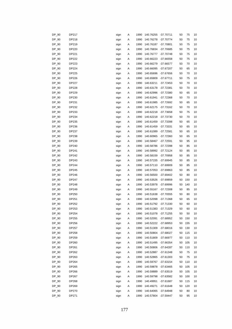
177

DP_90 DP217 sign A 1990 140.76255 -37.70711 50 75 10

DP_90 DP218 sign A 1990 140.76278 -37.70774 50 75 10

DP_90 DP219 sign A 1990 140.76187 -37.70801 50 75 10

DP_90 DP220 sign A 1990 140.76834 -37.70685 50 75 10

DP_90 DP221 sign A 1990 140.76777 -37.70748 50 75 10

DP_90 DP222 sign A 1990 140.66223 -37.66558 50 75 10

DP_90 DP223 sign A 1990 140.66279 -37.66577 50 70 10

DP_90 DP224 sign A 1990 140.66095 -37.67207 50 65 10

DP_90 DP225 sign A 1990 140.65696 -37.67656 50 70 10

DP_90 DP226 sign A 1990 140.65809 -37.67711 50 75 10

DP_90 DP227 sign A 1990 140.63211 -37.72453 50 70 10

DP_90 DP228 sign A 1990 140.63178 -37.72381 50 70 10

DP_90 DP229 sign A 1990 140.62996 -37.72380 50 65 10

DP_90 DP230 sign A 1990 140.61941 -37.72368 50 70 10

DP_90 DP231 sign A 1990 140.61985 -37.72692 50 65 10

DP_90 DP232 sign A 1990 140.62175 -37.73162 50 70 10

DP_90 DP233 sign A 1990 140.62218 -37.73658 50 75 10

DP_90 DP234 sign A 1990 140.62218 -37.73730 50 70 10

DP_90 DP235 sign A 1990 140.61459 -37.73398 50 65 10

DP_90 DP236 sign A 1990 140.61459 -37.73331 50 65 10

DP_90 DP237 sign A 1990 140.61089 -37.72581 50 65 10

DP_90 DP238 sign A 1990 140.60965 -37.72360 50 65 10

DP_90 DP239 sign A 1990 140.58467 -37.72591 50 95 10

DP_90 DP240 sign A 1990 140.58786 -37.72398 50 85 10

DP_90 DP241 sign A 1990 140.58992 -37.72124 50 85 10

DP_90 DP242 sign A 1990 140.58159 -37.70958 50 85 10

DP_90 DP243 sign A 1990 140.57155 -37.69945 50 85 10

DP_90 DP244 sign A 1990 140.57110 -37.69909 50 85 10

DP_90 DP245 sign A 1990 140.57053 -37.69863 50 85 10

DP_90 DP246 sign A 1990 140.56500 -37.69402 50 80 10

DP_90 DP247 sign A 1990 140.53526 -37.69859 50 150 10

DP_90 DP248 sign A 1990 140.53978 -37.69996 50 140 10

DP_90 DP249 sign A 1990 140.55167 -37.72308 50 85 10

DP_90 DP250 sign A 1990 140.51638 -37.70555 50 80 10

DP_90 DP251 sign A 1990 140.52098 -37.71368 50 65 10

DP_90 DP252 sign A 1990 140.51792 -37.71330 50 60 10

DP_90 DP253 sign A 1990 140.51383 -37.71329 50 60 10

DP_90 DP254 sign A 1990 140.51078 -37.71255 50 50 10

DP_90 DP255 sign A 1990 140.52091 -37.68952 50 150 10

DP_90 DP256 sign A 1990 140.52222 -37.68953 50 155 10

DP_90 DP257 sign A 1990 140.51309 -37.68016 50 130 10

DP_90 DP258 sign A 1990 140.50804 -37.68027 50 115 10

DP_90 DP259 sign A 1990 140.51809 -37.66977 50 110 10

DP_90 DP260 sign A 1990 140.51495 -37.66354 50 105 10

DP_90 DP261 sign A 1990 140.50806 -37.64287 50 110 10

DP_90 DP262 sign A 1990 140.52887 -37.61348 50 75 10

DP_90 DP263 sign A 1990 140.52865 -37.61303 50 75 10

DP_90 DP264 sign A 1990 140.59767 -37.63154 50 110 10

DP_90 DP265 sign A 1990 140.59878 -37.63465 50 105 10

DP_90 DP266 sign A 1990 140.59889 -37.63519 50 105 10

DP_90 DP267 sign A 1990 140.59798 -37.63582 50 100 10

DP_90 DP268 sign A 1990 140.49951 -37.61687 50 115 10

DP_90 DP269 sign A 1990 140.49271 -37.61648 50 120 10

DP_90 DP270 sign A 1990 140.64065 -37.64948 50 80 10

DP_90 DP271 sign A 1990 140.57804 -37.59447 50 95 10

178

DP_90 DP272 sign A 1990 140.57860 -37.59609 50 95 10

DP_90 DP273 sign A 1990 140.53705 -37.57466 50 115 10

DP_90 DP274 sign A 1990 140.52400 -37.57894 50 105 10

DP_90 DP275 sign A 1990 140.52104 -37.58010 50 95 10

DP_90 DP276 sign A 1990 140.52234 -37.57172 50 100 10

DP_90 DP277 sign A 1990 140.52394 -37.57056 50 105 10

DP_90 DP278 sign A 1990 140.50159 -37.55929 50 85 10

DP_90 DP279 sign A 1990 140.50646 -37.55913 50 110 10

DP_90 DP280 sign A 1990 140.78105 -37.70597 50 70 10

DP_90 DP281 sign A 1990 140.78456 -37.70598 50 75 10

DP_90 DP282 sign A 1990 140.76518 -37.70117 200 75 10

DP_90 DP283 sign A 1990 140.76404 -37.70206 200 75 10

DP_90 DP284 sign A 1990 140.76291 -37.70206 200 75 10

DP_90 DP285 Y N tr C 1990 140.76178 -37.70125 200 75 10

DP_90 DP286 sign A 1990 140.76291 -37.70152 200 75 10

DP_90 DP287 sign A 1990 140.76405 -37.70116 200 75 10

DP_90 DP288 sign A 1990 140.76064 -37.70206 200 75 10

DP_90 DP289 Y N tr C 1990 140.75871 -37.70151 200 75 10

DP_90 DP290 sign A 1990 140.75747 -37.70133 200 75 10

DP_90 DP291 sign A 1990 140.93204 -37.58691 50 70 10

DP_90 DP292 sign A 1990 140.47887 -37.61805 50 80 10

DP_90 DP293 sign A 1990 140.49871 -37.68411 50 75 10

DP_90 DP294 sign A 1990 140.92850 -37.61341 50 70 10

DP_90 DP295 sign A 1990 140.86882 -37.46652 50 65 10

DP_90 DP296 sign A 1990 140.87109 -37.46608 50 65 10

DP_90 DP297 sign A 1990 140.45643 -37.57216 200 120 10

DP_90 DP298 sign A 1990 140.49394 -37.55249 50 75 10

DP_90 DP299 sign A 1990 140.65276 -37.72622 50 70 10

DP_90 DP300 sign A 1990 140.88069 -37.47330 50 65 10

DP_90 MBFR01 sign A 1982 140.44965 -37.57122 200 105 20

DP_90 MBFR02 sign A 1979 140.45870 -37.57127 500 120 20

DP_93 an062 obs UC 1983 136.39222 -33.58207 500 290 10

DP_93 an063 obs UC 1993 136.39222 -33.58207 500 290 10

DP_93 an064 obs UC 1994 136.16862 -33.93882 750 160 20

DP_96_9 96_1 sign A 1996 140.71352 -37.71196 50 60 10

DP_96_9 96_10 sign A 1996 140.93212 -37.96957 50 40 10

DP_96_9 96_11 sign A 1996 140.53366 -37.57231 50 120 10

DP_96_9 96_12 sign A 1996 140.59901 -37.63528 50 105 10

DP_96_9 96_13 sign A 1996 140.93317 -37.58691 50 70 10

DP_96_9 96_14 sign A 1996 140.58992 -37.72160 50 85 10

DP_96_9 96_15 sign A 1996 140.59245 -37.71872 50 75 10

DP_96_9 96_16 sign A 1996 140.98520 -37.87539 50 55 10

DP_96_9 96_17 sign A 1996 140.98526 -37.87550 50 55 10

DP_96_9 96_18 sign A 1996 140.99823 -37.87514 50 55 10

DP_96_9 96_19 sign A 1996 140.93352 -37.96971 50 35 10

DP_96_9 96_2 sign A 1996 140.58843 -37.71294 50 85 10

DP_96_9 96_20 sign A 1996 140.94589 -37.96613 50 55 10

DP_96_9 96_21 sign A 1996 140.99881 -37.87494 50 55 10

DP_96_9 96_22 sign A 1996 140.95626 -37.96141 50 50 10

DP_96_9 96_23 sign A 1996 140.99910 -37.85390 50 60 10

DP_96_9 96_24 sign A 1996 140.76743 -37.70739 50 75 10

DP_96_9 96_25 sign A 1996 140.93204 -37.58691 50 70 10

DP_96_9 96_3 sign A 1996 140.94649 -37.96547 50 40 10

DP_96_9 96_4 sign A 1996 140.95697 -37.95953 50 40 10

DP_96_9 96_5 sign A 1996 140.94798 -37.96015 50 35 10

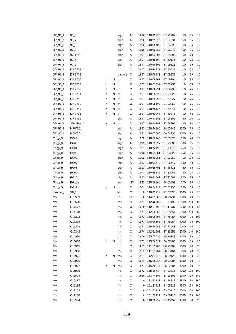
179

DP_96_9 96_6 sign A 1996 140.95776 -37.96962 50 35 10

DP_96_9 96_7 sign A 1996 140.95616 -37.97034 50 35 10

DP_96_9 96_8 sign A 1996 140.95106 -37.96993 50 35 10

DP_96_9 96_9 sign A 1996 140.93337 -37.96942 50 35 10

DP_96_9 97_1_a sign A 1997 140.93204 -37.58686 50 70 10

DP_96_9 97_5 sign A 1997 140.69104 -37.69115 10 75 10

DP_96_9 97_6 sign A 1997 140.69102 -37.69123 10 75 10

DP_96_9 DP 9701 tr C 1997 140.68828 -37.69223 10 75 10

DP_96_9 DP 9703 capture C 1997 140.68831 -37.69238 10 75 10

DP_96_9 DP 9708 Y N tr C 1997 140.68767 -37.69264 10 75 10

DP_96_9 DP 9737 Y N tr C 1997 140.69234 -37.69451 10 65 10

DP_96_9 DP 9750 Y N tr C 1997 140.68831 -37.69238 10 75 10

DP_96_9 DP 9751 Y N tr C 1997 140.68828 -37.69223 10 75 10

DP_96_9 DP 9752 Y N tr C 1997 140.69092 -37.69227 10 75 10

DP_96_9 DP 9753 Y N tr C 1997 140.69100 -37.69253 10 75 10

DP_96_9 DP 9754 Y N tr C 1997 140.69126 -37.69341 10 75 10

DP_96_9 DP 9771 Y N tr C 1997 140.68968 -37.69275 10 85 10

DP_96_9 DP 9789 sign A 1997 140.43951 -37.56352 50 100 10

DP_96_9 JFoulkes_1 Y N tr C 1997 140.94393 -37.96691 100 50 10

DP_96_9 NPWS01 sign A 1993 140.84360 -38.03748 2500 10 10

DP_96_9 NPWS02 sign A 1993 140.67805 -38.04233 1000 20 10

Grigg_9 BG02 sign A 1992 140.52140 -37.68375 150 140 10

Grigg_9 BG03 sign A 1992 140.73397 -37.70606 300 65 10

Grigg_9 BG04 sign A 1991 140.74190 -37.70878 250 65 10

Grigg_9 BG05 sign A 1992 140.61981 -37.73323 250 65 10

Grigg_9 BG06 sign A 1992 140.43951 -37.56352 50 100 10

Grigg_9 BG07 sign A 1993 140.94649 -37.96547 100 40 10

Grigg_9 BG08 sign A 1993 140.65791 -37.66733 50 75 10

Grigg_9 BG09 sign A 1993 140.69148 -37.69288 50 75 10

Grigg_9 BG10 sign A 1992 140.61903 -37.72061 500 65 10

Grigg_9 BG10a sign UC 1992 140.76860 -38.05809 100 10 10

Grigg_9 BG11 Y N tr C 1981 140.96912 -37.61230 500 65 10

Kemper_ SF_1 sf C 0 140.85713 -37.07035 1000 75 20

MV C10532 ms C 0 144.61605 -38.28734 2000 20 10

MV C10560 ms C 1971 142.46703 -37.31193 25000 260 600

MV C11127 ms C 1970 142.64400 -37.14737 2000 200 20

MV C11128 ms C 1971 142.55266 -37.08551 3000 200 60

MV C11393 ms C 1973 148.96396 -37.75984 5000 20 100

MV C11394 ms C 1973 148.96396 -37.75984 5000 20 100

MV C11398 ms C 1973 149.59255 -37.72065 2000 40 40

MV C12342 ms C 1974 142.51991 -37.13551 5000 240 160

MV C14986 ms C 1968 145.55053 -38.26747 1000 20 10

MV C15675 Y N ms C 1972 145.56327 -38.37486 1000 60 20

MV C15965 ms C 1962 141.53704 -38.23464 2000 70 20

MV C15966 ms C 1962 141.53704 -38.23464 2000 70 20

MV C15971 Y N ms C 1967 142.87215 -38.39125 1000 100 20

MV C15976 ms C 1971 145.30914 -38.22684 1000 10 5

MV C15977 Y N ms C 1971 145.30914 -38.22684 1000 10 5

MV C15979 ms C 1972 145.40714 -37.92316 2000 300 100

MV C16005 ms C 1969 143.74192 -38.53359 5000 300 150

MV C17187 ms C 0 151.23121 -33.66113 7500 160 160

MV C17188 ms C 0 151.23121 -33.66113 7500 160 160

MV C17189 ms C 0 151.23121 -33.66113 7500 160 160

MV C17190 ms C 0 151.23121 -33.66113 7500 160 160

MV C18534 ms C 0 148.20752 -37.45457 1500 160 20

180

MV C18544 ms C 1964 145.12202 -37.95049 2000 40 10

MV C18551 ms C 1964 145.09242 -37.99507 1500 10 5

MV C18553 ms C 1964 145.12202 -37.95049 2000 40 10

MV C18556 ms C 1960 145.14478 -37.95085 2000 40 20

MV C18608 ms C 0 145.05898 -37.96749 2000 20 10

MV C18615 ms C 1961 142.56949 -37.08303 2500 300 80

MV C18618 ms C 1975 145.51483 -37.65870 5000 120 100

MV C18619 ms C 1963 143.71273 -38.51986 3000 180 100

MV C18746 ms C 1973 145.09242 -37.99507 1500 10 5

MV C18952 ms C 1970 142.94133 -38.62260 3000 20 40

MV C18954 ms C 1964 145.12202 -37.95049 2000 40 10

MV C19442 ms C 1965 145.37193 -37.81723 2000 400 100

MV C19443 ms C 1964 145.12202 -37.95049 2000 40 10

MV C21564 ms C 1974 142.81483 -38.38854 3000 80 40

MV C21928 ms C 1973 142.82808 -38.57306 1000 10 10

MV C22169 ms C 1968 145.61689 -38.26376 2000 20 10

MV C23077 ms C 1978 147.98918 -37.87120 3000 20 40

MV C23157 Y N ms C 1968 142.64508 -37.19693 1000 220 20

MV C23483 ms C 1963 145.12271 -37.92347 2000 60 10

MV C23907 ms C 1980 141.25113 -38.16350 20000 40 40

MV C25688 Y N ms C 1982 144.12991 -38.43952 1000 60 20

MV C26318 ms C 1973 144.40302 -38.00890 1000 20 20

MV C26596 ms C 1977 142.28415 -37.17435 5000 220 20

MV C26613 ms C 1983 145.18495 -38.16776 2000 80 20

MV C27072 Y N ms C 1981 145.44556 -38.15077 1000 10 5

MV C27115 Y N ms C 1982 145.26546 -38.14194 1000 80 20

MV C27131 ms C 1978 148.81398 -37.66131 3000 140 60

MV C28024 ms C 1978 147.96660 -37.88400 3000 20 20

MV C28039 ms C 0 151.35426 -33.42836 7500 100 100

MV C29688 Y N ms C 1989 142.83989 -37.14629 100 220 20

MV C29689 ms C 1989 142.83989 -37.14629 100 220 20

MV C29707 Y N ms C 1991 148.71766 -37.73665 1000 60 20

MV C29751 ms C 1988 143.97161 -38.54060 3500 20 120

MV C29802 Y N ms C 1984 142.82808 -38.57306 1000 10 10

MV C5788 ms C 1867 145.37252 -37.94521 50000 140 500

MV C5794 ms C 1867 145.37252 -37.94521 50000 140 500

MV C5796 ms C 1981 144.64576 -37.89687 2500 20 10

MV C5797 ms C 1981 144.64576 -37.89687 2500 20 10

MV C5798 ms C 0 145.87741 -37.67172 5000 340 200

MV C5814 ms C 1932 145.12257 -38.37404 2500 40 20

MV C6889 ms C 1965 145.17533 -38.09552 2000 20 10

MV C697 ms C 1935 141.59497 -38.33349 5000 20 70

MV C698 ms C 1935 141.59497 -38.33349 5000 20 70

MV C699 ms C 1935 141.59497 -38.33349 5000 20 70

MV C700 ms C 1935 141.59497 -38.33349 5000 20 70

MV C701 ms C 1935 141.59497 -38.33349 5000 20 70

MV C702 ms C 1935 141.59497 -38.33349 5000 20 70

MV C703 ms C 1935 141.59497 -38.33349 5000 20 70

MV C704 ms C 1935 141.59497 -38.33349 5000 20 70

MV C705 ms C 1935 141.59497 -38.33349 5000 20 70

MV C706 ms C 1935 141.59497 -38.33349 5000 20 70

MV C714 ms C 1935 141.59497 -38.33349 5000 20 70

MV C715 ms C 1935 141.59497 -38.33349 5000 20 70

MV C716 ms C 1935 141.59497 -38.33349 5000 20 70

MV C7181 ms C 0 138.64880 -35.06596 750 370 30

181

MV C7194 ms C 1962 145.17533 -38.09552 2000 20 10

MV C7198 ms C 1962 145.17533 -38.09552 2000 20 10

MV C7220 ms C 1962 145.50605 -37.81360 2000 120 40

MV C7491 ms C 0 141.53704 -38.23464 2000 80 20

MV C761 ms C 1935 141.59497 -38.33349 5000 20 70

MV C762 ms C 1935 141.59497 -38.33349 5000 20 70

MV C9488 ms C 1969 142.61215 -37.23794 2500 300 200

MV C9526 ms C 1969 142.61979 -37.22612 1000 240 40

MV C9560 ms C 1970 146.30684 -39.02685 1000 40 60

NSW_PWS 11753-SEF ps C 1986 149.36585 -37.04413 100 740 20

NSW_PWS 11770-SEF ps C 1986 149.45816 -36.90797 100 320 20

NSW_PWS 12107-HO obs UC 1991 150.19832 -35.22224 1000 740 200

NSW_PWS 12160-SEF dig UC 1992 149.45472 -37.28925 1000 460 40

NSW_PWS 12488-SEF Y C 1978 149.76666 -37.28333 100 80 20

NSW_PWS 12493-SEF Y N Y C 1978 149.90948 -37.41230 100 200 20

NSW_PWS 12534-SEF Y N Y C 1982 149.76666 -37.28333 100 80 20

NSW_PWS 13945-SEF ps C 1994 149.72315 -36.98488 100 460 20

NSW_PWS 1438-SEF Y N hs C 1990 149.77690 -37.40107 100 120 20

NSW_PWS 15068-SEF dig UC 1986 149.96984 -36.73317 100 40 20

NSW_PWS 1663171/10 Y N rk C 1988 149.85583 -37.15905 100 40 20

NSW_PWS 19-BM rk UC 1991 151.38839 -33.50185 100 20 20

NSW_PWS 2174-SEF ps C 1991 149.41050 -37.12254 100 660 20

NSW_PWS 2688-NO K UC 1991 150.70618 -35.13107 100 40 20

NSW_PWS 2696-NO ? UC 1990 150.51202 -35.02087 1000 120 60

NSW_PWS 2697-NO ? UC 1990 150.51202 -35.02087 1000 120 60

NSW_PWS 343-SEF ps C 1989 149.80919 -37.32822 100 120 20

NSW_PWS 34442-HO ? UC 1985 151.23371 -33.67108 10000 160 160

NSW_PWS 345-SEF ps C 1989 149.80435 -37.31932 100 80 20

NSW_PWS 38239-HO sp UC 1994 152.32054 -32.39919 100 20 20

NSW_PWS 40027-HO ? UC 1990 151.35722 -33.49964 100 80 20

NSW_PWS 4004-NO Y Y hs C 1993 150.67647 -34.66803 100 580 20

NSW_PWS 401-SEF M UC 1991 149.61439 -36.88211 100 560 20

NSW_PWS 40307-HO ps C 1986 150.37019 -33.64400 100 860 20

NSW_PWS 40321-HO dig UC 1987 150.24004 -33.77008 100 700 20

NSW_PWS 40334-HO dig UC 1987 150.30706 -33.83602 100 360 20

NSW_PWS 40444-HO Y Y hs C 1986 150.36055 -33.64199 100 820 20

NSW_PWS 4293-SEF tr C 1988 149.62222 -37.21666 100 280 20

NSW_PWS 4294-SEF Y N tr C 1988 149.62222 -37.21666 100 280 20

NSW_PWS 4295-SEF Y N tr C 1988 149.62638 -37.21944 100 400 20

NSW_PWS 4296-SEF tr C 1988 149.62638 -37.21944 100 240 20

NSW_PWS 4297-SEF Y N tr C 1988 149.62499 -37.21639 100 280 20

NSW_PWS 4298-SEF tr C 1988 149.62499 -37.21639 100 280 20

NSW_PWS 4299-SEF tr C 1988 149.61389 -37.21388 100 240 20

NSW_PWS 4300-SEF tr C 1988 149.62222 -37.21666 100 280 20

NSW_PWS 4301-SEF tr C 1988 149.61666 -37.21250 100 240 20

NSW_PWS 4302-SEF Y N tr C 1988 149.61666 -37.21250 100 240 20

NSW_PWS 4303-SEF Y N tr C 1988 149.61389 -37.21388 100 240 20

NSW_PWS 4304-SEF tr C 1988 149.62499 -37.21639 100 280 20

NSW_PWS 4305-SEF ps C 1988 149.63305 -37.22499 100 320 20

NSW_PWS 4306-SEF Y N obs C 1988 149.85555 -37.15000 100 40 20

NSW_PWS 4307-SEF ps C 1988 149.64166 -37.22778 100 240 20

NSW_PWS 44459-035 dig UC 1979 151.28312 -33.59964 100 140 20

NSW_PWS 479-SEF ps C 1991 149.57745 -36.85137 100 680 20

NSW_PWS 485-SEF obs UC 1991 149.57745 -36.85137 100 680 20

NSW_PWS 4982-SEF Y Y hs C 1992 149.47776 -37.20424 100 500 20

182

NSW_PWS 5624-SEF obs UC 1992 149.95334 -36.74079 1000 60 40

NSW_PWS 58861-HO obs UC 1995 148.17662 -36.40746 100 480 20

NSW_PWS 60040-HO obs UC 1995 151.97989 -32.24490 100 100 20

NSW_PWS 62595-HO ps C 1995 149.47992 -37.01855 100 660 20

NSW_PWS 62596-HO scat UC 1995 149.50185 -36.99493 100 580 20

NSW_PWS 738-NO ? UC 1989 150.50606 -34.81972 100 140 20

NSW_PWS 805-SER Z UC 1990 150.50085 -35.02785 1000 180 60

NSW_PWS SABJ98071729 obs UC 1998 151.48580 -33.28574 1000 0 20

NSW_PWS SAWC99030500 Y N rk C 1998 150.21314 -35.78050 100 40 20

NSW_PWS SCLG9909160E dig A 1998 149.95162 -37.39233 1000 40 40

NSW_PWS SDMP96101403 obs UC 1996 149.60743 -37.34456 100 400 20

NSW_PWS SDMP97072307 rk UC 1997 150.70015 -34.38675 100 400 20

NSW_PWS SDMP99090305 obs UC 1999 150.63984 -34.38154 10000 440 100

NSW_PWS SDMP9909140F Y N obs C 1996 151.14422 -33.69502 100 160 20

NSW_PWS SDMP9909140G Y N tr C 1988 151.21662 -33.71503 100 160 20

NSW_PWS SDMPI0006863 obs UC 1999 150.62341 -34.53909 100 600 20





NSW_PWS SEXK9908053I obs UC 1993 150.48381 -35.22581 100 100 20

NSW_PWS SHXA99051918 ps UC 1997 149.73035 -36.89391 100 340 20

NSW_PWS SJBL00060500 Y N rk C 2000 151.28210 -33.70513 100 60 20

NSW_PWS SMCE9703170U obs UC 1996 149.61318 -37.20097 100 280 20

NSW_PWS SMCE97041813 obs UC 1994 149.97730 -36.54915 10000 60 200

NSW_PWS SNJR97060300 obs UC 1997 149.97516 -36.69699 100 40 20

NSW_PWS SPXEI0000010 Y N obs C 1983 150.39406 -35.52317 100 20 20

NSW_PWS SPXEI0000896 Y N hs C 1994 149.76069 -37.29954 1000 80 20

NSW_PWS SPXEI0000913 Y N tr C 1981 149.76485 -37.30061 1000 80 20

NSW_PWS SPXEI0000916 Y N tr C 1993 149.76630 -37.30022 1000 80 20

NSW_PWS SPXEI0000917 tr C 1981 149.76630 -37.30022 1000 80 20

NSW_PWS SPXEI0000929 hs C 1990 149.78028 -37.40099 1000 120 60

NSW_PWS SPXEI0000968 ps C 1989 149.80435 -37.31932 1000 80 20

NSW_PWS SPXEI0000980 ps C 1989 149.80919 -37.32822 1000 120 20

NSW_PWS SPXEI0000998 ps C 1991 149.82263 -37.38557 1000 160 40

NSW_PWS SPXEI0001021 tr C 1981 149.83611 -37.30595 1000 200 120

NSW_PWS SPXEI0001156 obs C 1972 149.93632 -37.43416 1000 40 20

NSW_PWS WD10664 Y N tr C 1977 151.28102 -33.59690 100 120 20

NSW_PWS WD13372 Y Y rk C 1977 151.21750 -33.64650 100 40 20

NSW_PWS WD14455 rk C 1972 151.28674 -33.57985 100 140 20

NSW_PWS WD1473 Y N obs C 1972 149.93632 -37.43416 100 40 20

NSW_PWS WD1648 Y N obs C 1973 149.94295 -37.40156 1000 40 20

NSW_PWS WD17769 rk C 1972 151.28104 -33.59600 100 120 20

NSW_PWS WD18429 dig UC 1981 151.19275 -33.69574 100 160 20

NSW_PWS WD2110 obs C 1977 151.28102 -33.59690 100 120 20

NSW_PWS WD21876 Y N rk C 1974 151.28068 -33.61403 100 120 20

NSW_PWS WD22579 Y N rk C 1986 149.93222 -37.18376 100 60 20

NSW_PWS WD24535 Y N rk C 1974 151.28104 -33.59600 100 140 20

NSW_PWS WD24536 rk C 1974 151.27003 -33.60757 100 140 20

NSW_PWS WD24691 tr C 1977 151.28102 -33.59690 100 120 20

NSW_PWS WD24692 tr C 1977 151.28102 -33.59690 100 120 20

NSW_PWS WD28864 obs UC 1978 151.19269 -33.64705 100 140 20

NSW_PWS WD28889 obs C 1982 151.27003 -33.60757 100 140 20

NSW_PWS WD29138 Y N rk C 1973 151.28674 -33.57985 100 140 20

NSW_PWS WD30626 ps C 1977 151.26453 -33.61291 100 160 20

183

NSW_PWS WD31738 obs C 1981 149.81950 -37.42259 1000 320 80

NSW_PWS WD34485 obs C 1973 149.94295 -37.40156 1000 40 20

NSW_PWS WD37008 ps C 1982 151.19172 -33.64162 100 120 20

NSW_PWS WD37216 Y Y obs C 1974 149.94401 -37.42856 1000 40 20

NSW_PWS WD38763 Y N rk C 1967 151.22902 -33.66290 100 160 20

NSW_PWS WD41639 Y N tr C 1980 151.26491 -33.59397 100 120 20

NSW_PWS WD41697 obs C 1973 149.94295 -37.40156 1000 40 20

NSW_PWS WD41970 Y N rk C 1979 151.26385 -33.64716 100 140 20

NSW_PWS WD46984 rk UC 1977 151.27430 -33.55533 100 0 30

NSW_PWS WD47047 rk C 1975 151.23651 -33.66571 1000 160 60

NSW_PWS WD47291 scat UC 1979 151.28312 -33.59964 100 140 20

NSW_PWS WD47292 dig UC 1979 151.23343 -33.65846 100 180 20

NSW_PWS WD47930 Y N rk C 1978 151.24744 -33.65866 100 120 20

NSW_PWS WD49226 Y N rk C 1967 151.21290 -33.71227 100 140 20

NSW_PWS WD5942 ps C 1983 151.29066 -33.59974 100 140 20

NSW_PWS WD7667 Y N rk C 1978 151.20928 -33.67885 100 180 20

NSW_PWS WD8448 rk C 1970 151.28102 -33.59690 100 120 20

NSW_PWS WD9550 Y N rk C 1982 151.27003 -33.60757 100 140 20

Rees_97 1 dig A 1997 141.64100 -38.38849 25 20 10

Rees_97 1002 dig A 1998 141.68540 -38.24040 25 70 10

Rees_97 1009 dig A 1998 141.68325 -38.23005 25 90 10

Rees_97 1011 dig A 1998 141.67719 -38.22377 25 100 10

Rees_97 1012 dig A 1998 141.67828 -38.21791 25 100 10

Rees_97 1023 dig A 1998 141.65954 -38.23041 25 80 10

Rees_97 1026 dig A 1998 141.66719 -38.22293 25 90 10

Rees_97 1028 dig A 1998 141.65288 -38.22031 25 45 10

Rees_97 1032 dig A 1998 141.65849 -38.20856 25 90 10

Rees_97 1034 dig A 1998 141.66966 -38.21187 25 90 10

Rees_97 1035 dig A 1998 141.67113 -38.21660 25 100 10

Rees_97 1043 dig A 1998 141.68115 -38.18838 25 70 10

Rees_97 1045 dig A 1998 141.67824 -38.18299 25 60 10

Rees_97 1047 dig A 1998 141.67083 -38.18415 25 70 10

Rees_97 1060 dig A 1998 141.64915 -38.18608 25 80 10

Rees_97 1071 dig A 1998 141.55264 -38.18229 25 70 10

Rees_97 109 dig A 1997 141.52691 -38.41412 25 100 10

Rees_97 113 dig A 1997 141.52698 -38.42430 25 40 10

Rees_97 1140 dig A 1998 141.42409 -38.36217 25 10 10

Rees_97 1146 dig A 1998 141.44325 -38.36007 25 40 10

Rees_97 1147 dig A 1998 141.44468 -38.36007 25 30 10

Rees_97 1149 dig A 1998 141.47885 -38.33560 25 70 10

Rees_97 1150 dig A 1998 141.47711 -38.33088 25 80 10

Rees_97 1151 dig A 1998 141.48113 -38.33311 25 70 10

Rees_97 1152 dig A 1998 141.48170 -38.33383 25 70 10

Rees_97 1153 dig A 1998 141.47740 -38.33268 25 70 10

Rees_97 1154 dig A 1998 141.47599 -38.33494 25 70 10

Rees_97 1157 dig A 1998 141.48862 -38.34097 25 70 10

Rees_97 1158 dig A 1998 141.48690 -38.34120 25 70 10

Rees_97 1160 dig A 1998 141.49860 -38.33755 25 80 10

Rees_97 1161 dig A 1998 141.49774 -38.33710 25 80 10

Rees_97 1162 dig A 1998 141.49890 -38.33845 25 80 10

Rees_97 1166 dig A 1998 141.44787 -38.32063 25 80 10

Rees_97 1168 dig A 1998 141.44957 -38.31882 25 85 10

Rees_97 1169 dig A 1998 141.42958 -38.27428 25 120 10

Rees_97 1171 dig A 1998 141.43158 -38.27450 25 110 10

Rees_97 1173 dig A 1998 141.42987 -38.27563 25 120 10

184

Rees_97 1174 dig A 1998 141.43190 -38.28058 25 110 10

Rees_97 1177 dig A 1998 141.43363 -38.28328 25 100 10

Rees_97 118 Y N dig A 1997 141.54422 -38.43215 25 40 10

Rees_97 121 dig A 1997 141.55253 -38.42400 25 50 10

Rees_97 122 Y N dig A 1997 141.55152 -38.42743 25 40 10

Rees_97 128 dig A 1997 141.54249 -38.42243 25 40 10

Rees_97 131 Y N dig A 1997 141.55445 -38.42281 25 60 10

Rees_97 133 dig A 1997 141.55017 -38.41959 25 70 10

Rees_97 144 dig A 1997 141.53185 -38.40067 25 90 10

Rees_97 145 dig A 1997 141.53170 -38.39798 25 90 10

Rees_97 146 dig A 1997 141.53419 -38.39606 25 110 10

Rees_97 148 dig A 1997 141.53190 -38.39256 25 90 10

Rees_97 15 dig A 1997 141.63669 -38.39311 25 10 10

Rees_97 16 dig A 1997 141.63820 -38.38337 25 20 10

Rees_97 17 dig A 1997 141.63936 -38.38427 25 20 10

Rees_97 187 dig A 1997 141.61003 -38.38226 25 40 10

Rees_97 188 dig A 1997 141.61553 -38.38286 25 30 10

Rees_97 189 dig A 1997 141.62356 -38.38471 25 30 10

Rees_97 19 dig A 1997 141.64047 -38.38084 25 20 10

Rees_97 191 dig A 1997 141.62535 -38.37547 25 30 10

Rees_97 192 dig A 1997 141.62712 -38.37700 25 20 10

Rees_97 193 dig A 1997 141.62985 -38.37571 25 30 10

Rees_97 194 dig A 1997 141.62899 -38.37356 25 30 10

Rees_97 20 dig A 1997 141.63990 -38.38156 25 20 10

Rees_97 203 dig A 1997 141.40490 -38.26671 25 140 10

Rees_97 204 dig A 1997 141.40351 -38.26347 25 130 10

Rees_97 205 dig A 1997 141.40295 -38.26654 25 130 10

Rees_97 206 dig A 1997 141.39986 -38.26520 25 120 10

Rees_97 207 dig A 1997 141.40099 -38.26276 25 120 10

Rees_97 208 dig A 1997 141.39639 -38.25863 25 110 10

Rees_97 211 dig A 1997 141.40716 -38.26292 25 140 10

Rees_97 212 dig A 1997 141.40652 -38.27004 25 150 10

Rees_97 214 dig A 1997 141.40735 -38.25553 25 130 10

Rees_97 215 dig A 1997 141.40011 -38.26907 25 120 10

Rees_97 216 dig A 1997 141.40012 -38.27123 25 120 10

Rees_97 217 dig A 1997 141.40240 -38.26978 25 130 10

Rees_97 218 dig A 1997 141.40779 -38.25192 25 120 10

Rees_97 219 * dig A 1997 141.63028 -38.39360 25 30 10

Rees_97 22 dig A 1997 141.63817 -38.38013 25 10 10

Rees_97 220 * dig A 1997 141.64560 -38.39108 25 10 10

Rees_97 221 * dig A 1997 141.64144 -38.38750 25 20 10

Rees_97 222 * dig A 1997 141.61195 -38.39343 25 40 10

Rees_97 223 * dig A 1997 141.55423 -38.42273 25 60 10

Rees_97 224 * dig A 1997 141.53153 -38.41959 25 70 10

Rees_97 225 * dig A 1997 141.44188 -38.29542 25 100 10

Rees_97 226 * dig A 1997 141.43705 -38.29048 25 100 10

Rees_97 227 * dig A 1997 141.43631 -38.28210 25 100 10

Rees_97 228 * dig A 1997 141.43423 -38.27742 25 100 10

Rees_97 229 * dig A 1997 141.43349 -38.26931 25 100 10

Rees_97 23 dig A 1997 141.64331 -38.39110 25 20 10

Rees_97 230 * dig A 1997 141.59743 -38.24264 25 50 10

Rees_97 231 * dig A 1997 141.58439 -38.24144 25 60 10

Rees_97 232 * dig A 1997 141.57933 -38.23678 25 60 10

Rees_97 233 * dig A 1997 141.56884 -38.23953 25 60 10

Rees_97 234 * dig A 1997 141.56583 -38.23531 25 60 10

185

Rees_97 235 * dig A 1997 141.55733 -38.27330 25 60 10

Rees_97 236 * dig A 1997 141.53356 -38.19680 25 45 10

Rees_97 237 * dig A 1997 141.53007 -38.18780 25 50 10

Rees_97 238 * dig A 1997 141.50824 -38.20124 25 70 10

Rees_97 239 * dig A 1997 141.51561 -38.24194 25 80 10

Rees_97 240 * dig A 1997 141.51592 -38.25438 25 80 10

Rees_97 241 * dig A 1997 141.52369 -38.25362 25 75 10

Rees_97 242 * dig A 1997 141.52813 -38.26757 25 80 10

Rees_97 243 * dig A 1997 141.53962 -38.27554 25 70 10

Rees_97 244 * dig A 1997 141.47850 -38.33367 25 70 10

Rees_97 245 * dig A 1997 141.47712 -38.33268 25 80 10

Rees_97 246 * dig A 1997 141.47885 -38.33493 25 70 10

Rees_97 247 * dig A 1997 141.47711 -38.33115 25 80 10

Rees_97 248 * dig A 1997 141.48824 -38.33687 25 90 10

Rees_97 249 * dig A 1997 141.49569 -38.33756 25 80 10

Rees_97 250 * dig A 1997 141.45302 -38.32097 25 80 10

Rees_97 251 * dig A 1997 141.59578 -38.29185 25 40 10

Rees_97 252 * dig A 1997 141.67092 -38.23115 25 85 10

Rees_97 253 * dig A 1997 141.66947 -38.22242 25 90 10

Rees_97 254 * dig A 1997 141.67944 -38.21407 25 105 10

Rees_97 255 * dig A 1997 141.69352 -38.20516 25 100 10

Rees_97 256 * dig A 1997 141.68914 -38.20050 25 90 10

Rees_97 257 * dig A 1997 141.66844 -38.21035 25 90 10

Rees_97 258 * dig A 1997 141.66637 -38.23325 25 85 10

Rees_97 259v dig A 1997 141.68893 -38.23857 25 75 10

Rees_97 260v dig A 1997 141.65850 -38.20923 25 90 10

Rees_97 261v dig A 1997 141.66741 -38.18440 25 80 10

Rees_97 262v dig A 1997 141.66528 -38.20199 25 95 10

Rees_97 263v dig A 1997 141.64009 -38.19492 25 70 10

Rees_97 264v dig A 1997 141.65964 -38.20968 25 90 10

Rees_97 27 dig A 1997 141.62662 -38.36821 25 20 10

Rees_97 3 dig A 1997 141.64143 -38.38624 25 20 10

Rees_97 30 dig A 1997 141.63032 -38.37260 25 20 10

Rees_97 44 dig A 1997 141.61468 -38.39080 25 30 10

Rees_97 47 dig A 1997 141.61122 -38.38820 25 30 10

Rees_97 5 dig A 1997 141.64239 -38.39128 25 20 10

Rees_97 6 dig A 1997 141.64353 -38.38965 25 15 10

Rees_97 63 dig A 1997 141.62195 -38.39752 25 40 10

Rees_97 66 dig A 1997 141.60262 -38.38618 25 60 10

Rees_97 68 dig A 1997 141.60172 -38.38843 25 40 10

Rees_97 7 dig A 1997 141.63921 -38.39319 25 10 10

Rees_97 80 dig A 1997 141.56777 -38.39527 25 30 10

Rees_97 93 dig A 1997 141.55302 -38.41337 25 70 10

Rees_97 94 dig A 1997 141.55348 -38.41408 25 70 10

Rees_97 95 dig A 1997 141.55326 -38.41553 25 70 10

Rees_97 A. Pritchard obs A 1997 141.63257 -38.38106 50 20 10

Rees_97 C. Dunn Y N obs A 1997 141.59219 -38.38488 50 35 10

Rees_97 Cleary Lands Y N obs A 1996 141.60781 -38.36317 50 20 10

Rees_97 David Largr obs A 1997 141.55325 -38.41345 50 70 10

Rees_97 George James Y N obs A 1997 141.60910 -38.38118 50 40 10

Rees_97 Glenda Smith Y N obs A 1997 141.63718 -38.38419 50 20 10

Rees_97 J. Hill/ K. Y N obs A 1996 141.62402 -38.38471 50 30 10

Rees_97 K. Holmes/K. Y N obs A 1996 141.63083 -38.37837 50 25 10

Rees_97 Keith Holmes Y N obs A 1996 141.62858 -38.38243 50 30 10

Rees_97 Keith Holmes obs A 1996 141.62004 -38.38879 50 30 10

186

Rees_97 Ken OÆConner Y N obs A 1998 141.62229 -38.38337 50 30 10








Rees_97 Ken OÆConner obs A 1998 141.63257 -38.38106 50 20 10



Rees_97 Ken O'Conner Y N obs A 1997 141.63257 -38.38106 50 20 10

Rees_97 Kevin Saunde obs A 1997 141.61027 -38.38433 50 40 10

Rees_97 Lyne Murrell Y N obs A 1997 141.54287 -38.40404 50 105 10

Rees_97 Max Lucas Y N obs A 1997 141.54192 -38.43108 50 40 10




Rees_97 Max Mc Lean Y N obs A 1993 141.55331 -38.42202 50 60 10

Rees_97 Michael Rees Y N obs A 1996 141.62004 -38.38879 50 30 10

Rees_97 Michael Rees Y N obs A 1997 141.54571 -38.40132 50 80 10

Rees_97 Mrs Menzel Y N obs A 1997 141.58200 -38.35699 50 30 10

Rees_97 Paul Banfiel Y N obs A 1997 141.61027 -38.38433 50 40 10

Rees_97 Portland Field Naturalists Y N obs A 1995 141.43495 -38.36123 50 20 10

Rees_97 Sheila Irvai Y N obs A 1995 141.54079 -38.43199 50 50 10

SA_FNS fns01 sign A 1976 138.70065 -34.93714 400 380 50

SA_FNS fns02 tr C 1968 138.76464 -34.99964 250 450 20

SA_FNS fns03 sign A 1968 138.71081 -35.27900 250 390 40

SA_FNS fns04 sign A 1969 138.72417 -35.27294 250 330 50

SA_FNS fns05 obs A 1969 138.71081 -35.27900 250 390 40

SA_FNS fns06 Y N tr C 1969 138.71081 -35.27900 250 390 40

SA_FNS fns07 Y N tr C 1969 138.68252 -35.30730 250 300 40

SA_FNS fns09 tr C 1970 138.68590 -35.26590 200 360 30

SA_FNS fns10 sign A 1972 138.21658 -35.64989 200 230 30

SA_FNS fns11 Y N tr C 1973 138.79244 -34.94336 250 590 40

SA_FNS fns12 sign A 1968 138.52649 -35.44754 400 400 40

SA_FNS fns13 sign A 1969 138.91703 -34.73549 750 480 100

SA_FNS fns14 sign A 1969 138.68590 -35.26590 200 360 30

SA_FNS fns15 sign A 1970 138.69982 -34.96688 200 500 50

SA_FNS fns16 Y N tr C 1982 138.68383 -35.26136 200 370 20

SA_FNS fns17 Y N tr C 1982 138.68590 -35.26590 200 360 30

SA_FNS fns18 Y N tr C 1985 138.69282 -35.09926 200 330 20

SA_FNS fns19 tr C 1988 138.67411 -35.02408 200 400 30

SA_FNS fns20 dig A 1974 136.86140 -35.89305 250 170 20

SA_FNS fns8 sign A 1970 138.68590 -35.26590 200 360 30

SAM 10139 Y N sp C 1975 137.19874 -35.83326 500 160 30

SAM 10163 sp C 1973 138.78306 -34.96662 500 480 40

SAM 10991 sp C 1979 137.96836 -35.78336 250 140 40

SAM 11011 sp C 1981 138.68054 -35.26129 100 360 20

SAM 11014 sp C 1981 138.68054 -35.26129 100 360 20

SAM 11015 Y N sp C 1981 138.68054 -35.26129 100 360 20

SAM 12217 sp C 1980 138.74952 -34.95158 250 450 50

SAM 12277 Y N sp C 1985 137.31057 -35.91048 250 20 10

SAM 12560 Y N sp C 1968 138.76464 -34.99964 250 460 30

SAM 12757 sp C 1985 138.67401 -35.02769 500 380 50

187

SAM 12804 Y N sp C 1983 138.69838 -35.01824 500 440 40

SAM 12998 Y N sp C 1983 136.89790 -35.75095 750 280 40

SAM 12999 Y N sp C 1986 138.49673 -35.62540 50 50 10

SAM 13010 Y N sp C 1983 138.68547 -35.08740 200 290 20

SAM 13244 Y Y sp C 1986 137.48278 -35.78356 250 50 10

SAM 13473 Y N sp C 1981 138.67434 -35.01597 200 400 30

SAM 13960 sp C 1987 137.63213 -35.64969 1000 50 40

SAM 13961 Y Y sp C 1987 137.24982 -35.91704 500 30 20

SAM 13962 Y N sp C 1987 136.91676 -35.98322 500 50 20

SAM 14060 Y N sp C 1987 136.89763 -35.78611 250 290 10

SAM 14424 Y N sp C 1987 136.92523 -35.78387 250 280 10

SAM 14472 Y N sp C 1987 138.52726 -35.42231 100 280 10

SAM 14593 sp C 1988 138.67070 -35.02853 200 410 20

SAM 14594 sp C 1988 138.67070 -35.02853 200 410 20

SAM 14595 sp C 1988 138.67070 -35.02853 200 410 20

SAM 14596 sp C 1988 138.67070 -35.02853 200 410 20

SAM 14597 Y N sp C 1988 138.67070 -35.02853 200 410 20

SAM 14598 Y N sp C 1988 138.67411 -35.02408 200 400 30

SAM 15365 Y N sp C 1989 137.00766 -35.98173 500 20 20

SAM 1601 sp C 1898 138.71688 -34.98343 1000 500 200

SAM 1602 sp C 1898 138.71688 -34.98343 1000 500 200

SAM 1603 sp C 1890 138.71688 -34.98343 1000 500 200

SAM 1604 sp C 1892 138.73295 -34.91702 1000 470 70

SAM 16156 Y Y sp C 1990 138.09880 -35.85259 250 70 20

SAM 2502 sp C 0 138.53229 -34.96629 1000 10 10

SAM 2578 sp C 1929 138.76655 -35.05016 1500 300 50

SAM 2665 sp C 1929 138.76655 -35.05016 1500 300 50

SAM 3006 Y N sp C 1931 138.81724 -34.83382 250 310 20

SAM 3011 Y Y sp C 1931 138.70042 -34.86682 750 100 70

SAM 3950 sp C 1902 138.73348 -35.01709 750 430 40

SAM 3951 sp C 1902 138.73348 -35.01709 750 430 40

SAM 3953 sp C 1902 138.73348 -35.01709 750 430 40

SAM 3991 Y Y sp C 1895 138.98325 -34.61670 1500 460 40

SAM 3992 sp C 1895 138.98325 -34.61670 1500 460 40

SAM 3993 sp C 1895 138.98325 -34.61670 1500 460 40

SAM 4567 sp C 1934 138.63526 -35.11708 750 190 60

SAM 4609 Y N sp C 1939 138.73348 -35.01709 750 430 40

SAM 4702 sp C 1936 138.74974 -35.50058 1500 10 10

SAM 4928 Y N sp C 1939 138.69997 -34.88304 750 130 70

SAM 5230 sp C 1893 138.73295 -34.91702 1000 470 70

SAM 5283 sp C 0 138.69998 -35.00024 1000 540 50

SAM 5620 Y N sp C 1946 138.61724 -35.28350 750 300 40

SAM 5833 sp C 1950 137.33269 -35.83344 50000 100 200

SAM 6032 sp C 1955 137.33269 -35.83344 50000 100 200

SAM 6054 sp C 1956 138.64910 -35.01729 750 310 50

SAM 6096 sp C 1957 138.64880 -35.06596 750 370 30

SAM 6194 sp C 1958 137.33269 -35.83344 50000 100 200

SAM 6201 sp C 1959 137.26595 -35.78333 2500 150 40

SAM 6271 Y N sp C 1959 138.63272 -35.31806 750 270 40

SAM 6290 sp C 1960 138.96703 -34.70028 1000 550 100

SAM 6292 Y N sp C 1960 138.53378 -35.53332 1000 50 40

SAM 6323 Y N sp C 1960 138.96703 -34.70028 1000 550 100

SAM 6816 Y N sp C 1966 138.64880 -35.06596 750 370 30

SAM 7251 sp C 1968 138.69998 -35.00024 1000 540 50

SAM 7252 sp C 1967 137.26595 -35.78333 2500 150 40

188

SAM 7254 sp C 1965 138.62560 -34.99610 500 300 50

SAM 7255 Y N sp C 1965 138.53394 -35.60002 1000 90 20

SAM 7264 sp C 1965 137.63216 -35.65059 1000 50 40

SAM 7265 Y N sp C 1965 137.21707 -35.97444 1000 10 10

SAM 777 sp C 0 138.69998 -35.00024 1000 540 50

SAM 7950 sp C 1969 137.36563 -35.74987 2000 80 40

SAM 8503 Y N sp C 1970 137.31676 -35.66609 500 170 30

SAM 8639 sp C 1969 138.78306 -34.96662 500 480 40

SAM 8640 sp C 1969 138.78306 -34.96662 500 480 40

SAM 8641 sp C 1969 138.78306 -34.96662 500 480 40

SAM 8642 sp C 1969 138.78306 -34.96662 500 480 40

SAM 8643 sp C 1969 138.78306 -34.96662 500 480 40

SAM 8992 sp C 1967 138.61721 -34.98331 750 100 70

SAM 9022 sp C 1973 137.33269 -35.83344 50000 100 200

SAM 9216 sp C 1973 137.26595 -35.78333 2500 150 40

SAM 9478 Y N sp C 1975 138.78306 -34.96662 500 480 40

SAM 9479 Y N sp C 1974 136.93339 -35.98296 500 40 10

SAM SAM 7948 sp UC 1968 136.28331 -33.64909 500 140 10

SAM SAM 8993 sp UC 1971 136.39222 -33.58207 500 290 10

SAM SAM02326 sp C 1927 140.78408 -37.83370 5000 50 30

SAM SAM02924 sp C 1930 140.96583 -37.99995 5000 10 20

SAM SAM03259 sp C 1932 140.78408 -37.83370 5000 50 30

SAM SAM05119 sp C 1944 140.69993 -37.56672 5000 70 10

SAM SAM05122 sp C 1944 140.69993 -37.56672 5000 70 10

SAM SAM05128 sp C 1944 140.69993 -37.56672 5000 70 10

SAM SAM05131 sp C 1944 140.48113 -37.60382 5000 225 100

SAM SAM05132 sp C 1944 140.48113 -37.60382 5000 225 100

SAM SAM06800 sp C 1965 140.38273 -37.58351 2500 20 100

SAM SAM07268 sp C 1965 139.92432 -37.36661 1500 20 100

SAM SAM08644 sp C 1970 140.76178 -37.70125 250 75 10

SAM SAM10284 Y N sp C 1979 140.66664 -37.66668 200 65 10

SAM SAM10285 Y N sp C 1979 140.75041 -37.70835 1000 75 10

SAM SAM11935 Y N sp C 1981 140.95458 -37.77800 250 65 10

SAM SAM11943 Y N sp C 1984 140.51666 -37.71483 500 45 20

SAM SAM11951 Y N sp C 1984 140.65052 -37.71981 500 70 10

SAM SAM11952 Y N sp C 1984 140.62325 -37.72694 500 65 10

SAM SAM11953 Y N sp C 1984 140.61646 -37.72331 500 65 10

SAM SAM12857 sp C 1984 140.85467 -37.47642 1000 65 10

SAM SAM12932 Y N sp C 1982 140.62663 -37.73281 500 65 20

Watts a EP_SF1 sf C 0 135.57109 -34.38494 2000 250 100

189

A2 Bioclimatic Profiles for Isoodon obesulus: the *. pro file calculated from 323 sites using BIOCLIM. PARAMETER

ME

AN

2.5%

5%

10%

25%

50%

75%

90%

95%

97.5

%

MA

X.

MIN

.

1. Annual Mean Temperature

13.5 12.3 12.5 12.8 13.1 13.4 13.8 14.5 15.8 16.4 16.7 11.9

2. Mean Diurnal Range

9.7 6.8 7.3 8.3 8.8 9.8 10.3 11.0 11.7 11.9 12.1 6.5

3. Isothermality 2/7 0.5 0.5 0.5 0.5 0.5 0.5 0.5 0.5 0.5 0.5 0.5 0.4

4. Temperature Seasonality (C of V)

1.2 0.9 0.9 1.0 1.1 1.2 1.3 1.4 1.5 1.5 1.6 0.9

5. Max Temperature of Warmest Period

24.5 21.9 22.2 22.4 23.1 24.6 25.6 26.4 27.4 27.8 28.7 21.5

6. Min Temperature of Coldest Period

4.8 2.8 2.9 3.3 4.2 4.9 5.5 6.1 7.0 8.0 8.5 1.2

7. Temperature Annual Range (5-6)

19.6 14.7 15.8 16.4 18.1 19.9 21.1 22.5 23.9 24.4 24.8 13.7

8. Mean Temperature of Wettest Quarter

10.6 7.5 7.8 8.2 9.0 9.8 11.1 12.5 17.7 19.8 20.5 7.3

9. Mean Temperature of Driest Quarter

17.1 10.1 11.1 13.4 16.7 17.6 18.3 18.6 19.3 19.7 21.2 8.4

10. Mean Temperature of Warmest Quarter

18.0 16.4 16.5 16.7 17.2 17.8 18.6 19.2 20.3 21.1 21.3 16.3

11. Mean Temperature of Coldest Quarter

9.3 7.6 7.7 8.0 8.9 9.3 9.7 10.5 11.3 11.6 11.9 7.1

12. Annual Precipitation

855 598 634 669 745 825 947 1055 1225 1260 1291 558

13. Precipitation of Wettest Period

27.0 16.0 17.0 20.0 22.0 27.0 30.0 34.0 36.0 37.0 40.0 15.0

14. Precipitation of Driest Period

5.0 0 0 0 1.0 1.0 11.0 15.0 16.0 16.0 17.0 0

15. Precipitation Seasonality (C of V)

32.0 11.0 12.0 14.0 19.0 31.0 45.0 51.0 57.0 60.0 62.0 11.0

16. Precipitation of Wettest Quarter

298 193 206 222 253 303 327 384 412 422 431 176

17. Precipitation of Driest Quarter

132 65 71 79 93 112 164 213 221 228 242 58

18. Precipitation of Warmest Quarter

142 63 68 78 98 118 169 235 312 368 385 58

19. Precipitation of Coldest Quarter

283 178 189 210 238 295 318 350 379 402 425 167

190

20. Annual Mean Radiation

15.4 14.3 14.4 14.6 14.8 15.3 16.2 16.5 16.7 16.8 17.1 14.0

21. Highest Period Radiation

25.6 24.0 24.1 24.2 24.8 25.5 26.2 27.1 27.3 27.4 27.5 23.5

22. Lowest Period Radiation

6.1 5.3 5.4 5.4 5.7 6.1 6.5 6.8 7.1 7.9 8.1 5.0

23. Radiation Seasonality (Cof V)

45.0 35.0 40.0 41.0 44.0 46.0 47.0 47.0 48.0 49.0 49.0 34.0

24. Radiation of Wettest Quarter

9.6 6.2 6.3 6.5 7.1 8.3 11.1 15.2 17.7 18.6 22.0 6.0

25. Radiation of Driest Quarter

21.4 11.5 12.5 14.3 21.1 22.2 23.1 24.0 24.4 24.6 24.7 9.9

26. Radiation of Warmest Quarter

22.7 21.1 21.2 21.4 21.8 22.4 23.6 24.3 24.6 24.8 25.4 20.6

27. Radiation of Coldest Quarter

7.9 6.8 6.9 7.0 7.3 7.6 8.4 8.8 9.5 9.8 9.9 6.6

28. Annual Mean Moisture Index

0.7 0.6 0.6 0.6 0.7 0.7 0.8 0.8 0.9 0.9 0.9 0.5

29. Highest Period Moisture Index

1.0 0.9 0.9 0.9 0.9 1.0 1.0 1.0 1.0 1.0 1.0 0.9

30. Lowest Period Moisture Index

0.2 0.1 0.1 0.1 0.1 0.2 0.3 0.4 0.4 0.5 0.5 0.1

31. Moisture Index Seasonality (C of V)

45.0 21.0 24.0 29.0 36.0 48.0 54.0 60.0 66.0 69.0 73.0 18.0

32. Mean Moisture Index of High Qtr. MI

1.0 1.0 1.0 1.0 1.0 1.0 1.0 1.0 1.0 1.0 1.0 0.9

33. Mean Moisture Index of Low Qtr. MI

0.3 0.1 0.1 0.1 0.2 0.2 0.4 0.5 0.5 0.6 0.6 0.1

34. Mean Moisture Index of Warm Qtr. MI

0.3 0.1 0.1 0.1 0.2 0.2 0.4 0.5 0.6 0.6 0.7 0.1

35. Mean Moisture Index of Cold Qtr. MI

1.0 0.9 0.9 1.0 1.0 1.0 1.0 1.0 1.0 1.0 1.0 0.9

191

A3 Validation of the Suitability Maps

Frequencies for 229 validation records compared to the indices in the suitability maps.

WEIGHTS

AND SUITABILITY INDICES

0 1 2 3 4 5 6 7 8 9 10

323 sites BIOMAP %records 10.5 33.6 11.8 12.2 31.9 0 %area 90.3 4.6 1.5 2.1 1.6 0 8 merged regions BIOMAP %records 30.1 12.7 11.8 21.4 21 3.1 %area 96.6 0.7 0.7 1 0.9 0.1 climate suitability map %records 10.5 14 5.2 11.4 9.2 12.2 11.4 15.3 8.7 2.2 %area 90.3 3.4 1.4 1.5 1.2 0.7 0.7 0.5 0.3 0weighted lithological association map

%records 0 0.4 12.2 5.7 81.7

%area 0.6 4.9 5.3 8.3 80.9 weighted regolith class map %records 0 1.3 0.9 45 52.8 %area 25.7 20.8 2.1 41.9 9.6 geologic suitability map %records 0 0 0 0 0 0.4 10 7 33.6 48.9 %area 0 0 0.9 0.3 0.8 28.7 24.6 9.1 27.7 7.9weighted 1788 tallest stratum dominant species map

%records 0.4 0.9 0 0 98.7

%area 0.4 19.4 8.9 0 0 71.3 weighted 1788 tallest stratum growth form map

%records 0 9.2 0 26.2 64.6

%area 0.4 0 33.9 0 21 44.7 weighted 1788 tallest stratum density map

%records 0 0 0 57.6 42.4

%area 0.4 0 10.5 0 64.1 25.1 weighted 1788 lower stratum growth form map

%records 1.3 0 7.4 19.7 10.9 60.7

%area 4.6 3.3 40.1 3.1 15.5 33.5 1788 vegetation suitability map %records 0 0 0 0.4 0.9 0 0 34.5 8.7 55.5 %area 0.4 0 0 2.3 13.7 13.5 5.9 35.4 10.1 18.8weighted 1988 tallest stratum dominant species map

%records 1.7 0.4 62.4 0 0 35.4

%area 1.2 14.4 44.1 0 0 40.3 weighted 1988 tallest stratum growth form map

%records 1.7 0 42.4 0 15.3 40.6

%area 1.2 0 59.3 0 15 24.5 weighted 1988 tallest stratum density map

%records 1.7 0 12.2 27.5 11.8 46.7

%area 1.2 0 29.1 4 22.5 43.3 weighted 1988 lower stratum growth form map

%records 64.2 0 12.2 13.5 2.6 7.4

%area 40 3.1 31.2 1.5 6.1 18.1 1988 vegetation suitability map %records 1.7 0 0 6.6 55.9 0 12.7 10.5 4.4 8.3 %area 1.2 0 0 13.2 36.6 11.4 14.9 9.9 2.3 10.41788 habitat suitability map %records 0 0 0 10.9 11.8 17.5 19.2 16.2 17 7.4 %area 10.1 17.7 26.4 19.1 20 3.5 1.5 0.9 0.6 0.21988 habitat suitability map %records 0 2.6 10.9 17 17.5 20.1 23.6 7.9 0.4 0 %area 21.3 27.8 22.4 14.4 10.5 2.3 0.9 0.4 0.1 0

193

A4 Stratified Sampling Maps

A4.1 Digital Elevation Models

194

A4.2 System used to reclassify digital elevation models into local relief classes.

The figures represent elevation values in metres used to reclassify each DEM during the stratification process.

Code 1000 2000 3000 4000 Local relief low low to intermediate intermediate to high high Typical landforms depressions plains low dunes/low hillslopes high dunes/upper hillslopes The Bluff 87-109 109-131 131-150 - Brooksby Lane 91-3 93-97 - - Burr Slopes South 82-98 98-105 105-118 118-139 Byrnes 67-70 70-77 - - Diagonal Road 66-70 70-77 - - Wild Dog Flat 31-40 40-49 49-60 - Glencoe Hill 76-98 98-128 128-149 - Gower 40-52 52-61 61-74 - Grundys Lane 64-66 66-70 70-76 - Hacket Hill 60-71 71-87 87-98 - The Heath 67-70 - - - Honans 46-67 67-74 74-85 - Kays 96-108 108-118 118-134 134-150 Lake Leake 95-100 100-115 - - Longs 75-80 80-86 86-90 90-108 Marshes 75-77 77-79 79-83 - Mt McIntyre 91-104 104-125 125-158 - McRosties 79-98 98-132 132-162 - Mt Lyon 94-99 99-103 103-114 - Native Wells 66-79 79-97 97-119 119-140 Overland Track 79-84 84-98 98-109 - Paltridges 67-70 - - - Honeysuckle Flat 36-42 42-69 69-85 - Wandilo 63-69 69-80 80-90 - Mt Watch 137-142 142-172 172-189 - Whennans 74-90 90-108 108-130 130-135 Windy Hill North 137-144 144-157 157-177 - Windy Hill South 68-78 68-91 91-155 - Woolwash 76-82 82-88 88-119 119-155

195

A4.3 Local Relief Classes for sampling based on reclassified digital elevation models.

196

A4.4 Vegetation sampling units, based on the Department of Housing and Urban Development vegetation map.

N

Eucalyptus baxteri (100)

Eucalyptus obliqua (200)

Eucalyptus ovata/E. viminalis (300)

shrubs (400)

reedbed/sedgeland (500)

other (600)

0 10 km

197

A4.5 Number of fires since 1957 and number of years since burning in 1998.

ArcView shapefiles of fire blocks and archived forestry reports of prescribed burning and bushfires were provided by ForestrySA.

Number of fires since 1957.

198

A4.5 continued. Number of years since burning in 1998.

199

A4.6 Sampling Units: Combinations of Relief, Vegetation and Fire Classes.

When the relief, vegetation and fire maps of Appendices A3, A4 and A5 were overlaid, 254 unique sampling units were formed. With it not being possible to display all classes in one map, the 17 units with the largest aggregate areas (each >1.5% of the study area) are shown here. In the legend, ‘other’ refers the other 237 sampling classes that are too small to represent at this map scale.

N

1105

1134

1314

1405

1505

2105

2114

2123

2124

2132

2133

2143

2405

3123

3124

3132

3134

other0 10 km

201

A5 Observations of Isoodon obesulus Diggings A general observation about diggings as an indicator of bandicoot presence is that they are are less ephemeral than scats and footprints. Bandicoot nests persist longer than diggings, even when they are abandoned but they are very difficult to find. Scats are rarely seen and they may last one week, or perhaps more, while footprints and tail drag marks on diggings are apparent for only a few days and not after rainfall. To make specific observations of the aging of diggings, a sample of 20 fresh diggings was marked with flags on 25 April 1998 and revisited on 8 July 1999 and 28 September 1999. Notes made about the diggings included the formation of a crust on the spoil heap, which proved to be a good indicator of the approximate age of the diggings. Three age classes were apparent from the general and specific observations above: 1) fresh diggings are recognised by friable soil on the spoil heap and are approximately less than two weeks old; 2) recent diggings have a crust formed on the spoil heap with unconsolidated soil beneath and they are aged approximately two weeks to two months; and 3) old diggings, which have a completely consolidated spoil heap are older than two months.

25 April 1999 8 July 1999 28 Sept 1999 digging number

Depth (cm)

condition Depth(cm)

condition Depth (cm)

condition

1 10 Fresh. Spoil heap soft and friable.

5 Spoil hard, disturbed and obscured by more recent diggings.

3 Spoil obscure, moss.


6.5 Spoil hard, moss and dicot germinating.

6 Spoil obvious, hard, moss.


10 Spoil hard, moss and sticks in hole.

10 Spoil obvious, hard.


15 Spoil hard, leaves in hole.

15 Spoil hard.


5 Spoil hard with moss growing.

4 Spoil obvious, hard


6 Spoil hard, moss and Drosera.

6 spoil obvious, hard, Drosera.


8.5 Spoil hard, leaves in hole.

6.5 Spoil obvious, hard, sticks, leaves.


4 Spoil hard, orchid germinating.

3.5 Spoil obvious, hard.


16 Spoil hard, moss and Drosera growing.



4 Spoil hard, Drosera germinating.

4 Spoil obvious, hard, Drosera.


12 Spoil hard. 10 Spoil obvious, hard.


14 Spoil hard, moss growing.

13 Spoil obvious, hard, Drosera, orchid.


5 Spoil hard, Drosera germinating



9.5 spoil hard, Drosera germinating.




3.5 Spoil obscure.


12 Spoil hard, Acacia germinating.



13.5 Spoil hard, Drosera and orchid germinating.

9.5 Spoil obvious, hard, Drosera.


11 Spoil hard, moss and orchid germinating.

9.5 Spoil obvious, hard, orchid.



4.5 Spoil obvious, hard.


4.5 Spoil hard, Drosera germinating.

2.5 Spoil obvious, hard, Drosera.

203

A6 Criteria for Field Evaluation of Drainage

from McDonald et al. (1990) pp 151-152.

Drainage is a useful term to summarize local soil wetness conditions, that is, it provides a statement about soil and site drainage likely to occur in most years. It is affected by a number of attributes, both internal and external, that may act separately or together. Internal attributes include soil structure, texture, porosity, hydraulic conductivity, and water-holding capacity, while external attributes are source and quality of water, evapotranspiration, gradient and length of slope and position in the landscape.

1. Very poorly drained Water is removed from the soil so slowly that the water remains at or near the surface for most of the year. Surface flow, ground-water and subsurface flow are major sources of water, although precipitation may be important where there is a perched water table and precipitation exceeds evapotranspiration. Soils have a wide range in texture and depth, and often occur in depressed sites. Strong gleying and accumulation of surface organic matter are usually features of most soils in this class.

2. Poorly drained Water is removed very slowly in relation to supply. Subsurface and/or groundwater flow, as well as precipitation, may be a significant water source. Seasonal ponding resulting from runon and insufficient outfall also occurs. A perched water table may be present. Soils have a wide range in texture and depth; many have horizons that are gleyed, mottled, or possess orange or rusty linings of root channels. All horizons remain wet for periods of several months.

3. Imperfectly drained Water is removed only slowly in relation to supply. Precipitation is the main source if available water storage capacity is high, but subsurface flow and/or groundwater contribute as available water storage capacity decreases. Soils have a wide range in texture and depth. Some horizons may be mottled and/or have orange or rusty linings of root channels, and are wet for periods of several weeks.

4. Moderately well drained Water is removed from the soil somewhat slowly in relation to supply, due to low permeability, shallow water table, lack of gradient, or some combination of these. Soils are usually medium to fine in texture. Significant additions of water by subsurface flow are necessary in coarse-textured soils. Some horizons may remain wet for as long as one week after water addition.

204

5. Well drained

Water is removed from the soil readily but not rapidly. Excess water flows downward readily into underlying moderate permeable material or laterally as subsurface flow. The soils are often medium in texture. Some horizons may remain wet for several days after water addition.

6. Rapidly drained

Water is removed from the soil rapidly in relation to supply. Excess water flows downward rapidly if underlying material is highly permeable. There may be rapid subsurface lateral flow during heavy rainfall provided there is a steep gradient. Soils are usually coarse-textured, or shallow, or both. No horizon is normally wet for more than several hours after water addition.

205

A7 Observations of Xanthorrhoea australis and Nesting by Isoodon obesulus

It has been noted that Isoodon obesulus in the South East nests under specimens of Xanthorrhoea australis that possess well-developed skirts of living and dead foliage reaching down to the ground (Paull 1995). It seems that these umbrella-like canopies provide protection from predators and camouflage bandicoot nests. In fact, I. obesulus nests are very difficult to locate because they are so well hidden.

Following a control burn in Honan Block C in August 1997, observations were made of Xanthorrhoea australis and I. obesulus nests along a belt transect 4 m wide by 100 m long. The presence/absence of I. obesulus nests, which were still completely visible following the fire at the base of some X. australis, was recorded along with the height of the main stem measured from the ground to the base of the apical shoot. Isoodon obesulus nests were located at the base of 40 out of 269 individual X. australis and no other nests were seen along the transect. Furthermore, it was observed that the individual X. australis with nests at their bases had stem heights between 35 cm and 75 cm while shorter and taller plants were not used for nesting. This is clearly important for understanding the ecological relationships between I. obesulus and vegetation in its habitat and it also has implications for fire management, which are discussed in Chapters 4 and 5.

5

15 25 35 45 55 65 75 85

0

5

10

15

20

25

30

stem height cm

NESTNO NEST

207

A8 Field survey data

Data highlighted in bold were excluded from analysis because no evidence of Isoodon obesulus was found in those remnants.

Variables are described in Table 4.2.

Site

_id

Land

syst

em

PR

ES

AB

UN

D

RE

LIE

F

LFO

RM

DR

AIN

SO

ILTE

X

CO

LOU

R

AS

SO

C

G_V

EG

SR

VE

G15

VE

G10

_15

VE

G5_

10

VE

G2_

5

VE

G1_

2

VE

G0_

1

N_F

IRE

F_A

GE

XA

NS

CO

RE

LITT

ER

GR

AM

S

FOR

BS

MO

SS

blu.1 MBU 0 0 1000 slope 5 S brown eucbax pteesc 2 1 4 2 3 3 6 1 5 4 3 1 1 4 blu.2 MBU 0 0 1000 slope 5 S dark gray eucbax pteesc 2 3 3 2 1 1 6 1 5 3 1 2 2 3 blu.3 MBU 0 0 3000 slope 5 S brown eucbax pteesc 2 1 4 2 1 1 3 1 5 3 1 2 3 2 blu.4 MBU 0 0 2000 slope 5 S very dark gray eucbax pteesc 3 1 3 3 2 2 6 1 5 5 1 1 1 5 blu.5 MBU 0 0 2000 slope 4 C brown eucvim other 2 1 4 2 2 1 1 1 5 1 1 4 4 2 bro.1 YOU 0 0 2000 plain 4 LS black eucbax pteesc 2 1 1 3 3 3 9 2 4 1 5 1 1 2 bro.2 DMR* 0 0 1000 plain 4 LS black eucbax pteesc 2 1 2 1 2 4 9 2 4 1 5 1 1 3 bur.1 MBU 0 0 4000 slope 5 S brown eucbax pteesc 3 1 2 3 2 3 5 3 3 4 4 2 2 2 bur.2 MBU 0 0 4000 slope 5 S dark gray eucbax pteesc 3 1 3 2 2 3 6 2 5 3 4 1 1 2 bur.3 MBU 0 0 4000 slope 5 S brown eucbax pteesc 2 1 4 2 1 3 7 2 5 3 3 2 1 1 bur.4 MBU 0 0 4000 slope 5 S very dark gray eucbax pteesc 2 1 1 4 2 4 8 2 5 3 4 1 1 2 bur.5 MBU 0 0 3000 slope 5 S very dark gray eucbax pteesc 3 1 2 4 2 4 8 2 5 3 4 1 1 1 bur.6 MBU 0 0 3000 slope 5 S brown eucbax pteesc 3 1 4 2 2 3 5 3 3 3 3 2 1 4 bur.7 MBU 0 0 1000 depression 4 S dark gray eucbax pteesc 2 1 4 2 2 3 6 3 3 3 3 1 1 2 bur.8 MBU 0 0 3000 plain 4 S very dark gray eucbax pteesc 3 2 3 2 2 2 6 3 3 3 3 1 1 3 bur.9 MBU 0 0 3000 slope 4 S very dark gray eucbax pteesc 3 1 1 1 2 3 7 2 5 3 4 1 1 2 bur.10 MBU 0 0 1000 depression 4 S black eucbax pteesc 2 1 1 4 1 4 8 2 5 3 3 1 1 3 byr.1 KLN 1 3 1000 plain 4 S brown shrubs lepto_mel 2 1 1 1 2 4 7 1 5 2 1 1 1 4 byr.2 KLN 1 2 1000 plain 4 S dark gray shrubs lepto_mel 2 1 1 1 2 3 7 1 5 1 1 2 1 4 byr.3 KLN 0 0 1000 plain 4 S very dark gray eucvim other 3 1 4 2 1 1 6 1 5 2 4 1 1 1 byr.4 KLN 1 3 1000 plain 4 S brown shrubs other 2 1 1 1 1 3 7 1 5 2 1 1 1 1 byr.5 KLN 1 2 1000 plain 4 S dark gray eucvim other 3 1 2 2 1 2 7 1 5 2 5 1 1 2 byr.6 NGW* 0 0 2000 plain 4 S very dark gray eucvim other 3 2 3 2 2 2 2 1 5 2 4 1 1 2 dia.1 YOU 0 0 1000 depression 1 L black reed/sedge reed 1 1 1 1 1 3 10 1 5 1 5 1 1 1 dia.2 YOU 1 1 1000 plain 4 LS black eucbax xanaus 2 1 1 3 2 4 6 1 5 6 1 1 1 4 dia.3 YOU 1 1 1000 plain 4 S very dark gray eucbax xanaus 2 1 1 2 2 3 7 1 5 5 1 1 1 1 dia.4 YOU 1 2 1000 slope 4 LS black eucbax xanaus 2 1 1 2 2 2 7 1 5 5 1 1 1 3

208

dia.5 YOU 0 0 1000 plain 3 L black other other 3 1 2 2 3 2 9 1 5 1 2 4 1 2 dia.6 YOU 0 0 1000 plain 4 S black eucova pteesc 2 1 1 3 2 2 8 1 5 2 5 1 1 3 dia.7 YOU 1 2 2000 slope 5 S dark gray eucbax lepto_mel 3 1 1 2 1 3 6 1 5 2 4 1 1 2 dia.8 YOU 1 2 1000 plain 4 L black eucbax lepto_mel 3 1 1 2 2 3 7 1 5 3 1 1 1 2 dia.9 YOU 0 0 1000 depression 2 L black reed/sedge reed 1 1 1 1 1 1 9 1 5 1 2 1 1 1 dia.10 YOU 1 2 2000 slope 5 S very dark gray other pteesc 2 1 1 3 2 4 9 1 5 3 5 1 1 5 dia.11 YOU 1 1 1000 plain 4 S black other xanaus 3 1 1 3 2 3 7 1 5 5 1 1 1 3 dia.12 YOU 0 0 1000 depression 1 C very dark gray reed/sedge sedge 1 1 1 1 1 1 10 1 5 1 2 5 1 1 dia.13 YOU 1 2 1000 plain 3 CS brown other other 2 4 3 2 3 2 8 1 5 2 5 4 1 2 dog.1 CRL 1 1 3000 slope 5 S very dark gray eucbax xanaus 2 1 1 3 2 1 4 4 1 2 3 1 1 1 dog.2 CRL 1 2 3000 slope 5 S very dark gray eucbax pteesc 2 1 1 3 1 3 8 5 3 3 2 1 1 1 dog.3 MSA* 0 0 2000 slope 5 CS brown eucbax pteesc 3 2 4 2 2 2 4 6 3 2 1 3 2 1 dog.4 CRL 0 0 2000 plain 4 S very dark gray eucbax pteesc 2 1 4 3 2 1 6 6 2 1 4 1 1 1 dog.5 CRL 0 0 2000 slope 4 S dark gray eucbax pteesc 3 2 4 2 2 2 4 3 5 1 4 2 1 2 dog.6 MSA* 0 0 1000 plain 4 S brown eucobl pteesc 2 1 4 2 3 2 3 5 3 1 4 2 1 2 dog.7 CRL 0 0 2000 slope 5 S very dark gray eucbax pteesc 3 1 3 1 2 2 5 5 4 1 4 1 1 1 dog.8 CRL 0 0 3000 slope 5 S dark gray eucbax pteesc 3 1 4 3 2 2 5 5 3 1 4 1 1 1 dog.9 CRL 0 0 2000 slope 5 S very dark gray eucbax pteesc 3 1 3 2 2 1 7 5 4 1 4 1 1 1 dog.10 CRL 0 0 1000 plain 4 S brown eucbax pteesc 2 1 3 2 3 4 4 6 2 1 4 1 1 2 dog.11 CRL 0 0 2000 plain 4 S dark gray eucbax pteesc 3 1 2 4 2 1 2 4 5 2 2 1 1 1 dog.12 CRL 1 1 2000 slope 4 S very dark gray eucbax pteesc 3 1 3 3 2 4 7 5 3 2 4 1 1 1 dog.13 CRL 1 1 1000 depression 4 S dark gray eucbax pteesc 2 1 1 3 2 4 8 2 5 1 4 1 1 2 dog.14 CRL 1 1 2000 slope 5 S dark gray eucbax xanaus 3 2 3 3 2 3 6 2 5 2 3 2 1 2 dog.15 CRL 0 0 3000 slope 5 S very dark gray eucbax pteesc 3 3 3 3 2 4 7 5 3 1 2 2 1 4 dog.16 CRL 0 0 2000 plain 4 S very dark gray eucbax pteesc 3 2 4 2 2 2 5 5 3 2 3 1 1 1 dog.17 CRL 0 0 1000 plain 4 S brown eucbax pteesc 3 2 4 2 2 2 4 4 5 2 2 1 1 2 dog.18 CRL 0 0 1000 plain 4 S brown eucbax pteesc 2 1 4 3 4 4 4 6 2 1 1 1 1 3 dog.19 CRL 0 0 1000 plain 3 S brown eucobl pteesc 2 1 4 3 2 2 3 5 4 1 1 3 3 3 dog.20 CRL 0 0 2000 plain 4 S very dark gray eucbax pteesc 3 2 4 2 3 2 6 2 5 2 2 1 1 1 dog.21 CRL 1 1 3000 slope 5 S very dark gray eucbax pteesc 3 1 4 2 2 3 7 5 3 3 3 1 1 4 dog.22 CRL 0 0 2000 slope 5 S very dark gray eucbax pteesc 3 1 4 3 3 2 7 5 3 1 3 1 1 2 gle.1 MBU 1 2 3000 slope 5 S brown eucobl pteesc 4 1 3 3 2 2 8 1 5 3 4 2 1 3 gle.2 MBU 1 1 3000 slope 4 S dark gray eucbax xanaus 3 1 1 3 2 3 8 4 3 2 4 1 1 1 gle.3 MBU 1 1 2000 slope 4 S dark gray eucbax pteesc 2 1 4 1 1 2 8 4 3 4 4 2 1 2 gle.4 MBU 1 1 2000 slope 4 S black eucbax pteesc 3 1 3 4 1 1 9 3 5 3 5 1 1 1 gle.5 MBU 1 1 1000 slope 4 S brown eucobl pteesc 2 1 1 4 4 2 3 3 5 3 3 2 2 3 gow.1 MBU 1 2 3000 slope 5 S brown eucobl pteesc 2 1 2 4 2 2 7 1 5 4 2 2 2 3 gow.2 MBU 0 0 1000 depression 4 C brown eucobl other 2 1 1 4 2 1 1 1 5 1 1 5 1 2 gow.3 MBU 1 1 3000 slope 5 S brown eucbax pteesc 2 1 2 4 1 2 8 1 5 5 4 1 1 1 gow.4 MBU 0 0 1000 slope 4 C brown eucova pteesc 2 1 4 2 2 1 6 1 5 3 2 2 3 3 gru.1 YOU 1 1 2000 slope 4 S very dark gray eucova pteesc 2 1 4 2 3 2 6 3 3 1 4 1 3 3 gru.2 YOU 1 1 2000 slope 4 S black eucbax pteesc 2 1 4 1 2 4 5 4 3 2 4 1 1 4 gru.3 YOU 1 3 2000 depression 4 C black shrubs reed 1 1 1 1 4 4 6 4 3 1 1 5 2 2 gru.4 YOU 1 1 2000 plain 4 LS black eucbax pteesc 2 1 1 4 2 4 7 3 4 1 5 1 1 2 gru.5 YOU 1 1 2000 plain 4 S very dark gray eucbax pteesc 2 1 4 1 2 2 6 3 3 1 4 1 1 2

209

gru.6 YOU 1 1 3000 plain 3 L black eucova lepto_mel 2 1 1 3 2 4 6 4 2 1 3 1 1 2 gru.7 YOU 1 1 3000 plain 4 CS very dark gray eucbax pteesc 2 1 4 2 2 3 7 3 3 1 4 2 1 3 gru.8 YOU 0 0 3000 slope 4 CS black eucbax pteesc 2 2 4 1 2 4 7 3 4 1 4 1 2 3 gru.9 YOU 0 0 3000 slope 4 LS black eucvim pteesc 2 2 4 1 2 1 6 4 4 1 4 2 2 3 gru.10 YOU 0 0 3000 depression 4 LS black shrubs lepto_mel 1 1 1 1 3 5 3 4 4 1 1 5 2 2 gru.11 YOU 0 0 2000 plain 4 CS brown eucbax pteesc 3 1 4 2 2 1 6 4 2 2 3 1 2 2 gru.12 YOU 1 1 3000 slope 4 LS black eucbax pteesc 2 1 1 3 1 4 8 3 3 2 5 1 2 3 gru.13 YOU 1 1 2000 plain 4 C dark gray eucova lepto_mel 2 1 3 4 2 2 5 3 3 1 3 1 2 2 gru.14 YOU 1 2 3000 depression 5 LS black other other 2 1 1 4 3 2 2 4 2 1 5 1 1 4 gru.15 YOU 1 1 2000 depression 4 LS black shrubs sedge 1 1 1 1 4 4 4 4 3 1 1 1 1 5 hak.1 YOU 1 1 1000 plain 4 LS black eucbax pteesc 2 1 1 4 3 3 5 4 4 1 1 1 1 2 hak.2 YOU 1 1 1000 plain 4 S dark gray eucbax xanaus 2 1 2 4 2 2 7 6 2 3 2 1 1 2 hak.3 YOU 0 0 1000 plain 4 L black eucova lepto_mel 1 1 1 4 2 4 6 6 4 1 4 1 1 2 hak.4 YOU 1 2 1000 plain 3 CS brown eucova pteesc 1 1 1 3 2 4 6 4 4 1 4 2 1 1 hak.5 YOU 1 1 1000 depression 1 LS black shrubs sedge 1 1 1 1 1 4 3 5 4 1 2 2 1 3 hak.6 YOU 0 0 1000 depression 1 L black reed/sedge reed 1 1 1 1 3 5 9 6 2 1 4 2 2 1 hak.7 YOU 0 0 1000 depression 3 C black reed/sedge lepto_mel 1 1 1 1 1 1 2 6 4 1 5 5 2 1 hak.8 YOU 0 0 2000 plain 4 S black eucbax pteesc 2 1 1 3 1 2 6 5 4 3 4 1 1 1 hak.9 YOU 1 1 2000 slope 4 S black eucbax pteesc 1 1 1 4 2 2 8 6 2 1 4 1 1 1 hak.10 YOU 0 0 3000 slope 5 S brown eucbax pteesc 2 1 4 2 2 1 3 5 4 1 1 3 2 1 hak.11 YOU 1 2 1000 plain 4 S very dark gray eucbax pteesc 2 1 1 4 2 3 7 4 4 3 4 1 1 1 hak.12 YOU 1 2 1000 plain 4 L black eucbax pteesc 2 1 1 4 3 2 6 6 2 2 5 1 1 1 hak.13 YOU 0 0 1000 plain 4 S very dark gray eucbax pteesc 1 1 1 4 2 2 6 6 4 3 4 1 1 2 hak.14 YOU 0 0 1000 plain 4 CS very dark gray eucova pteesc 2 1 1 4 2 4 6 4 4 1 4 2 1 1 hak.15 YOU 0 0 1000 depression 2 C black reed/sedge reed 1 1 1 1 1 5 6 4 4 1 4 1 1 3 hak.16 YOU 0 0 1000 depression 2 CS very dark gray shrubs lepto_mel 1 1 1 1 1 4 6 6 2 1 1 1 1 1 hak.17 YOU 0 0 1000 depression 4 CS brown eucova lepto_mel 1 1 1 3 3 4 5 6 4 1 1 1 1 3 hak.18 YOU 1 1 2000 plain 4 S very dark gray eucbax xanaus 2 1 1 3 2 3 7 4 4 4 2 1 1 2 hak.19 YOU 1 1 2000 plain 4 S very dark gray eucbax pteesc 3 1 2 3 2 2 7 6 2 3 2 1 1 1 hak.20 YOU 0 0 3000 slope 5 S brown eucbax xanaus 1 1 4 2 2 2 5 5 4 2 2 2 2 1 hak.21 YOU 0 0 1000 plain 4 LS black eucbax pteesc 1 1 4 2 1 2 8 5 4 1 5 1 2 1 hak.22 YOU 0 0 1000 depression 3 C black reed/sedge reed 1 1 1 1 1 2 4 4 4 1 1 2 5 1 hak.23 YOU 0 0 2000 plain 4 S very dark gray eucbax xanaus 3 1 4 2 1 2 2 4 4 3 4 1 1 1 hak.24 YOU 0 0 1000 plain 4 S very dark gray eucbax lepto_mel 2 1 4 2 2 2 4 4 4 2 1 1 1 2 hak.25 YOU 1 1 2000 plain 4 S very dark gray eucbax pteesc 1 1 4 2 1 3 7 5 4 1 4 1 2 2 hak.26 YOU 1 1 2000 plain 4 S very dark gray eucbax xanaus 2 1 4 2 1 2 3 4 4 4 4 1 1 1 hak.27 YOU 0 0 1000 depression 4 L black shrubs lepto_mel 1 1 1 1 1 5 5 4 4 1 3 1 1 4 hak.28 YOU 1 1 2000 plain 4 S very dark gray eucbax pteesc 2 1 4 3 1 3 5 4 4 3 3 1 2 1 hak.29 YOU 1 1 2000 plain 4 S very dark gray eucbax xanaus 3 1 2 3 2 2 6 5 4 4 2 1 1 2 hak.30 YOU 0 0 1000 plain 4 CS black eucbax pteesc 2 1 4 3 1 1 4 4 4 1 4 1 1 1 hak.31 YOU 0 0 2000 plain 4 L black eucbax pteesc 2 1 4 2 2 4 8 5 4 1 4 1 1 2 hak.32 YOU 1 1 2000 plain 4 S black eucbax lepto_mel 3 1 3 3 1 3 7 4 4 2 4 1 1 1 hak.33 YOU 1 1 2000 plain 4 S very dark gray eucbax pteesc 2 1 3 1 1 2 8 4 4 3 4 1 1 1 hak.34 YOU 0 0 1000 depression 2 L black reed/sedge reed 1 1 1 1 1 5 6 4 4 1 5 1 1 1 hak.35 YOU 1 1 1000 plain 4 S very dark gray eucbax pteesc 2 1 4 2 2 3 6 4 4 2 4 1 1 3

210

hak.36 YOU 0 0 1000 depression 2 LS black reed/sedge reed 1 1 1 1 3 5 3 4 4 1 1 2 4 4 hak.37 YOU 1 3 1000 plain 5 S very dark gray eucbax xanaus 2 1 3 3 2 3 7 4 4 3 4 1 2 1 hak.38 YOU 1 1 1000 depression 4 S black shrubs sedge 1 1 1 1 1 4 2 4 4 1 1 2 1 3 hak.39 YOU 0 0 2000 slope 5 S very dark gray eucbax pteesc 2 1 4 2 2 2 4 5 4 2 3 2 1 2 hea.1 KLN 0 0 1000 plain 4 S dark gray eucova lepto_mel 3 2 3 2 2 3 6 2 4 1 4 1 1 1 hea.2 KLN 1 1 1000 plain 4 S brown shrubs lepto_mel 3 1 1 1 1 2 6 2 4 1 1 1 1 1 hea.3 KLN 0 0 1000 plain 4 S dark gray eucvim lepto_mel 3 2 3 1 1 2 6 2 4 2 4 1 1 2 hea.4 KLN 1 1 1000 plain 4 S brown eucvim pteesc 2 1 3 4 2 3 4 2 4 1 4 1 1 1 hea.5 KLN 1 1 1000 plain 4 S gray eucvim lepto_mel 2 2 3 2 2 3 7 2 4 2 4 1 1 1 hon.1 YOU 1 1 1000 plain 3 CS black eucbax xanaus 3 1 3 4 2 2 6 3 2 6 4 1 1 1 hon.2 YOU 0 0 2000 plain 2 C brown eucova pteesc 2 1 4 2 2 1 1 2 2 1 1 5 2 2 hon.3 YOU 1 1 2000 slope 4 S dark gray eucbax xanaus 2 1 1 3 2 2 7 3 3 5 2 1 1 2 hon.4 YOU 0 0 1000 depression 2 L black reed/sedge reed 1 1 1 1 1 3 8 3 2 1 2 4 1 1 hon.5 YOU 0 0 2000 slope 4 CS brown eucbax xanaus 3 1 4 2 2 2 5 2 2 3 1 4 1 1 hon.6 YOU 1 1 3000 plain 4 S dark gray eucbax xanaus 3 1 1 3 3 2 6 2 2 5 1 1 1 3 hon.7 YOU 0 0 1000 plain 4 L black other lepto_mel 2 1 1 3 3 3 6 2 2 3 1 1 1 4 hon.8 YOU 1 1 3000 plain 4 S very dark gray eucbax xanaus 3 1 3 3 2 2 4 3 1 2 1 1 1 1 hon.9 YOU 1 1 3000 depression 4 L black shrubs lepto_mel 2 1 1 1 2 4 6 3 1 2 1 4 1 1 hon.10 YOU 1 1 2000 plain 4 S very dark gray other pteesc 3 1 2 3 2 2 7 3 1 2 1 1 1 3 hon.11 YOU 1 2 3000 plain 4 S dark gray other xanaus 2 1 1 4 2 4 8 1 5 6 3 1 2 4 hon.12 YOU 1 1 3000 plain 4 CS black eucbax lepto_mel 3 1 1 3 2 2 7 2 2 5 1 1 1 4 hon.13 YOU 0 0 3000 depression 3 L black reed/sedge reed 1 1 1 1 3 5 9 1 5 1 1 1 1 3 hon.14 YOU 0 0 1000 depression 1 L black reed/sedge reed 1 1 1 1 1 1 3 1 5 1 1 1 1 1 hon.15 YOU 0 0 3000 plain 4 S very dark gray eucbax xanaus 3 1 1 3 2 2 7 3 3 5 2 1 1 3 hon.16 YOU 0 0 1000 depression 1 L black reed/sedge other 2 1 1 1 1 1 4 2 2 1 5 5 1 1 hon.17 YOU 0 0 1000 slope 4 CS very dark gray eucbax pteesc 2 1 1 4 1 1 1 2 1 1 4 1 1 1 hon.18 YOU 0 0 2000 slope 5 S dark gray eucbax xanaus 3 1 2 4 2 2 7 2 1 2 3 2 1 1 hon.19 YOU 0 0 2000 slope 4 S very dark gray eucbax xanaus 2 1 1 4 2 3 5 2 1 3 1 1 1 3 hon.20 YOU 0 0 2000 plain 4 L black eucbax lepto_mel 2 1 1 4 2 4 4 3 1 2 1 1 1 3 hon.21 YOU 1 1 1000 depression 2 L black shrubs lepto_mel 1 1 1 1 4 5 8 1 5 1 1 2 1 4 hon.22 YOU 1 1 1000 plain 4 LS black other pteesc 2 1 1 4 3 5 9 3 3 1 4 1 1 2 hon.23 YOU 0 0 3000 slope 5 S dark gray eucbax pteesc 3 1 1 4 2 2 5 5 2 2 1 2 2 2 hon.24 YOU 1 1 3000 slope 5 S dark gray eucbax xanaus 3 1 2 4 2 1 3 4 1 2 2 1 1 1 hon.25 YOU 1 1 1000 slope 4 S very dark gray eucbax pteesc 2 1 1 1 2 2 7 4 2 2 4 1 1 2 hon.26 YOU 1 1 1000 slope 4 S dark gray eucbax xanaus 3 1 1 3 1 2 7 3 2 4 4 1 1 2 hon.27 YOU 1 1 1000 slope 4 LS black eucbax pteesc 2 1 2 3 1 2 5 3 1 2 3 1 1 1 hon.28 YOU 0 0 1000 plain 4 S black eucbax pteesc 2 1 1 3 2 2 4 3 1 1 2 1 1 2 hon.29 MBU* 1 1 1000 slope 4 S very dark gray eucvim pteesc 1 4 4 2 2 1 8 4 1 1 5 3 2 1 hon.30 YOU 0 0 3000 slope 4 S very dark gray eucbax lepto_mel 2 1 1 4 2 2 5 4 1 3 2 1 2 2 hon.31 YOU 1 1 1000 slope 4 S very dark gray eucbax xanaus 2 1 1 4 2 4 7 1 5 6 3 1 1 4 hon.32 YOU 0 0 1000 depression 1 C black reed/sedge sedge 1 1 1 1 1 1 8 4 1 1 5 5 2 1 hon.33 YOU 1 1 2000 plain 4 CS dark gray eucbax pteesc 2 1 4 2 2 4 8 3 2 3 4 1 1 3 hon.34 YOU 1 1 3000 plain 4 S black eucbax xanaus 2 1 1 4 1 3 7 3 2 3 4 1 1 1 hon.35 YOU 0 0 2000 depression 3 C brown shrubs lepto_mel 2 1 1 1 1 3 3 3 1 1 1 3 2 2 hon.36 YOU 1 1 1000 depression 3 C very dark gray shrubs lepto_mel 2 1 1 1 1 4 8 2 1 2 2 3 1 3

211

hon.37 YOU 1 1 1000 plain 4 S very dark gray shrubs xanaus 2 1 1 1 1 4 5 2 2 6 1 1 1 3 hon.38 YOU 0 0 3000 slope 4 S very dark gray eucbax xanaus 3 1 4 3 2 3 5 2 2 5 3 1 1 4 hon.39 YOU 1 1 2000 slope 4 S very dark gray eucbax xanaus 2 1 1 3 2 3 8 1 5 4 3 1 1 4 hon.40 YOU 1 1 1000 depression 2 S very dark gray shrubs lepto_mel 2 1 1 1 1 3 9 2 2 4 1 1 1 1 hon.41 YOU 1 1 3000 slope 4 S dark gray eucbax xanaus 3 1 1 3 1 1 4 2 1 3 1 1 1 2 hon.42 YOU 1 1 3000 slope 5 S dark gray eucobl pteesc 2 1 4 1 3 2 4 1 5 1 1 2 2 4 hon.43 YOU 1 1 2000 slope 5 S dark gray eucbax pteesc 3 1 4 1 1 2 6 5 2 2 3 1 2 2 hon.44 YOU 0 0 2000 plain 4 S black eucbax pteesc 2 1 4 2 2 2 3 3 3 1 2 1 2 2 hon.45 YOU 0 0 3000 plain 4 S black eucbax xanaus 2 1 1 4 2 4 4 1 5 6 3 1 1 3 hon.46 YOU 0 0 1000 slope 5 S very dark gray eucbax xanaus 2 1 2 3 1 1 3 2 1 2 2 1 1 1 hon.47 YOU 0 0 3000 slope 4 S very dark gray eucbax xanaus 2 1 1 3 1 3 3 2 1 2 2 2 1 1 hon.48 YOU 0 0 2000 plain 4 S very dark gray eucbax xanaus 3 1 1 3 2 4 6 2 3 5 1 2 2 3 hon.49 YOU 1 1 1000 plain 4 S very dark gray eucbax xanaus 2 1 1 4 2 2 7 1 5 6 4 1 1 2 hon.50 YOU 0 0 1000 depression 2 C black shrubs lepto_mel 2 1 1 1 2 4 9 2 3 1 1 5 1 1 hon.51 YOU 0 0 1000 plain 4 CS black eucova pteesc 2 1 2 4 2 3 7 3 1 1 1 4 2 2 kay.1 MBU 0 0 3000 slope 5 S brown eucbax pteesc 3 1 1 2 2 3 6 3 1 1 3 1 1 1 kay.2 MBU 1 2 2000 slope 5 S brown eucbax pteesc 4 1 1 4 3 2 5 6 2 2 1 1 1 2 kay.3 MBU 0 0 1000 plain 4 CS brown eucbax pteesc 3 1 4 2 2 2 3 6 2 2 3 1 2 1 kay.4 MBU 0 0 1000 slope 4 CS brown eucobl other 4 1 1 3 3 1 3 5 4 3 1 4 2 2 kay.5 MBU 0 0 3000 slope 5 S brown eucbax pteesc 4 1 3 1 2 3 10 6 3 2 4 1 1 1 kay.6 MBU 0 0 2000 slope 4 S very dark gray eucbax pteesc 3 1 2 3 2 4 9 3 2 1 3 1 1 2 kay.7 MBU 0 0 3000 slope 5 S very dark gray eucbax pteesc 2 1 1 2 2 5 9 3 2 1 3 1 1 2 kay.8 MBU 0 0 4000 plain 4 S very dark gray other pteesc 2 1 1 4 4 4 3 5 4 1 5 1 1 4 kay.9 MBU 0 0 3000 slope 5 S gray eucbax pteesc 3 1 1 3 2 4 9 4 4 1 5 1 1 1 kay.10 MBU 0 0 3000 slope 4 LS very dark gray eucbax pteesc 2 1 1 3 2 4 9 4 4 2 5 1 1 1 kay.11 MBU 0 0 4000 slope 5 CS brown eucbax pteesc 3 1 2 4 2 2 4 4 4 1 2 4 1 2 kay.12 MBU 0 0 1000 slope 4 S dark gray eucbax pteesc 2 1 2 3 2 3 8 6 2 1 4 1 1 1 kay.13 MBU 0 0 3000 slope 4 S very dark gray eucbax pteesc 3 1 2 2 2 4 8 4 2 2 3 1 1 2 llk.1 EDW 0 0 2000 slope 5 LS very dark gray eucbax pteesc 1 1 3 4 2 3 9 1 5 1 5 1 1 1 lon.1 MBU 1 1 4000 slope 4 S very dark gray eucbax pteesc 3 1 3 2 2 2 7 2 5 5 4 1 1 4 lon.2 MBU 1 1 4000 slope 5 S brown eucbax xanaus 3 2 3 3 2 3 6 3 5 6 1 1 2 4 lon.3 MBU 0 0 4000 slope 4 CS brown eucobl xanaus 3 1 2 3 2 3 4 3 5 5 2 1 2 3 lon.4 MBU 0 0 4000 depression 1 LS black shrubs lepto_mel 1 1 1 1 4 5 5 3 5 1 1 1 1 5 lon.5 MBU 1 1 2000 plain 4 L black eucova pteesc 3 1 1 3 3 3 7 4 5 2 3 1 1 2 lon.6 MBU 1 1 3000 plain 3 L very dark gray shrubs xanaus 2 1 1 1 1 4 8 3 5 5 1 2 1 4 lon.7 MBU 1 1 3000 slope 4 S very dark gray eucbax pteesc 3 1 2 3 1 2 6 4 5 5 1 1 1 4 lon.8 MBU 0 0 1000 depression 4 CS brown eucvim other 2 4 3 2 2 4 5 3 5 1 2 2 1 1 lon.9 MBU 1 1 3000 slope 4 L black eucova pteesc 1 4 3 3 2 4 7 3 5 1 5 1 1 1 mar.1 YOU 1 1 3000 plain 4 CS very dark gray eucvim pteesc 2 1 1 4 3 3 8 1 5 1 5 1 1 1 mar.2 YOU 0 0 1000 depression 1 L black shrubs sedge 1 1 1 1 4 4 8 1 5 2 2 3 1 4 mar.3 YOU 0 0 1000 depression 2 L black reed/sedge reed 1 1 1 1 1 3 9 1 5 1 1 1 1 1 mar.4 YOU 0 0 2000 plain 4 S black shrubs xanaus 3 1 1 1 1 3 7 1 5 3 1 2 1 2 mar.5 YOU 1 2 3000 plain 4 LS black eucbax xanaus 2 1 1 3 1 3 6 2 4 5 1 1 1 1 mar.6 YOU 0 0 2000 plain 4 LS black eucbax xanaus 3 1 1 2 2 2 8 2 4 5 1 1 1 1 mar.7 YOU 0 0 3000 plain 4 LS black shrubs lepto_mel 2 1 1 1 3 5 6 1 5 6 1 1 1 4

212

mar.8 YOU 0 0 1000 depression 2 L black reed/sedge reed 1 1 1 1 1 3 10 1 5 1 5 1 1 1 mar.9 YOU 1 2 1000 plain 4 LS black eucbax pteesc 2 1 2 3 2 4 5 1 5 1 4 1 1 1 mar.10 YOU 1 1 2000 depression 2 L black reed/sedge sedge 1 1 1 1 1 1 9 1 5 1 1 1 1 1 mar.11 YOU 0 0 3000 plain 3 LS black shrubs xanaus 2 1 1 1 1 3 7 1 5 6 1 1 1 2 mar.12 YOU 0 0 2000 plain 3 L black eucbax xanaus 3 1 1 3 2 3 7 1 5 6 1 1 1 2 mar.13 YOU 0 0 1000 depression 1 L black reed/sedge reed 1 1 1 1 1 1 10 1 5 1 4 1 1 1 mar.14 YOU 1 1 3000 plain 4 LS black eucbax xanaus 3 1 1 2 1 3 8 1 5 5 1 1 1 2 mar.15 YOU 0 0 1000 depression 2 L black reed/sedge reed 1 1 1 1 1 2 10 1 5 1 4 1 1 1 mar.16 YOU 0 0 3000 plain 4 LS black other pteesc 1 1 4 2 4 4 4 1 5 1 1 1 1 5 mar.17 YOU 1 1 2000 plain 4 S very dark gray eucbax other 2 1 1 4 3 3 7 2 4 3 2 1 1 1 mar.18 YOU 1 1 2000 depression 4 S very dark gray other lepto_mel 2 1 1 2 2 4 9 1 5 2 1 1 1 4 mar.19 YOU 0 0 1000 depression 2 L black reed/sedge reed 1 1 1 1 1 1 10 1 5 1 1 1 1 1 mar.20 YOU 1 1 3000 slope 5 S brown eucvim pteesc 2 4 3 1 2 1 5 1 5 2 5 1 1 1 mar.21 YOU 0 0 2000 plain 4 S black eucbax pteesc 2 1 1 3 3 2 8 1 5 1 5 1 1 1 mar.22 YOU 0 0 1000 depression 3 CS black shrubs lepto_mel 1 1 1 1 2 5 9 1 5 1 1 1 1 4 mar.23 YOU 0 0 3000 plain 3 C very dark gray shrubs lepto_mel 2 1 1 1 2 4 10 1 5 3 1 4 1 2 mar.24 YOU 1 1 2000 plain 3 L black shrubs xanaus 2 1 1 1 1 4 7 1 5 6 1 1 1 4 mar.25 YOU 0 0 3000 plain 4 LS black eucbax xanaus 3 1 1 4 3 4 8 1 5 6 2 1 1 4 mar.26 YOU 0 0 2000 plain 4 CS very dark gray eucbax xanaus 3 1 1 4 2 4 5 1 5 6 4 1 1 1 mar.27 YOU 0 0 1000 plain 4 S very dark gray eucvim xanaus 3 1 1 4 2 4 6 1 5 6 5 1 1 1 mar.28 YOU 1 1 2000 plain 4 CS dark gray eucvim pteesc 3 1 1 4 3 2 4 1 5 3 4 1 1 2 mar.29 YOU 0 0 3000 plain 3 LS black eucvim sedge 1 1 1 4 4 2 4 1 5 1 2 1 1 4 mci.1 MBU 0 0 3000 plain 4 S black eucbax pteesc 2 1 1 3 2 4 8 3 4 1 5 1 1 2 mci.2 MBU 1 1 3000 slope 4 L very dark gray eucbax pteesc 1 1 4 2 1 4 9 3 4 2 5 1 1 2 mci.3 MBU 1 1 3000 slope 4 LS very dark gray eucbax pteesc 3 1 1 3 1 2 9 3 4 3 4 1 1 1 mci.4 MBU 0 0 2000 plain 3 LS black eucova other 2 1 1 3 4 3 5 3 4 1 5 1 1 2 mci.5 MBU 0 0 1000 depression 2 L black reed/sedge reed 1 1 1 1 1 2 5 3 4 1 2 2 2 1 mcr.1 MBU 1 1 2000 slope 5 LS very dark gray eucbax other 3 1 1 2 2 3 8 2 4 2 1 1 1 2 mcr.2 MBU 1 2 2000 slope 5 S dark gray other pteesc 3 1 4 2 3 3 7 2 4 1 1 2 1 2 mcr.3 MBU 1 2 2000 slope 5 S very dark gray eucbax other 2 1 1 2 2 2 9 2 4 3 1 1 1 2 mcr.4 MBU 0 0 2000 plain 4 LS black eucbax lepto_mel 2 1 1 2 3 4 9 2 4 1 4 1 1 4 mcr.5 MBU 1 1 1000 slope 4 S very dark gray other pteesc 2 2 1 3 3 3 7 2 4 2 4 1 1 3 mcr.6 YOU* 1 2 1000 plain 3 CS black eucova pteesc 2 1 1 2 3 4 6 2 4 1 4 1 1 1 mcr.7 MBU 0 0 3000 slope 3 C brown other pteesc 1 1 1 4 1 1 1 2 4 1 1 4 2 2 mtl.1 YOU 0 0 1000 depression 2 L black reed/sedge reed 1 1 1 1 1 1 8 2 5 1 2 1 1 3 mtl.2 YOU 0 0 3000 slope 4 S very dark gray other pteesc 2 1 3 2 2 2 8 2 5 4 4 1 1 1 mtl.3 YOU 0 0 2000 slope 4 LS very dark gray eucbax pteesc 3 1 2 3 2 2 8 2 5 3 5 1 1 1 mtl.4 YOU 0 0 2000 plain 4 S very dark gray other xanaus 3 1 1 2 2 3 8 2 5 6 1 1 1 5 mtl.5 YOU 0 0 1000 slope 4 S very dark gray other pteesc 2 1 1 2 2 5 9 2 5 3 3 1 1 5 mtl.6 YOU 0 0 3000 slope 4 S very dark gray eucbax xanaus 2 1 1 2 3 2 8 2 5 5 1 1 1 4 mtl.7 YOU 0 0 3000 depression 4 LS very dark gray shrubs xanaus 2 1 1 1 2 4 7 2 5 1 1 1 1 4 mtl.8 YOU 0 0 1000 plain 4 LS very dark gray other xanaus 2 1 1 1 2 4 8 2 5 5 1 1 1 2 nat.1 MBU 1 1 3000 slope 5 S very dark gray eucbax pteesc 3 1 3 3 2 2 8 4 4 5 3 1 1 1 nat.2 MBU 1 2 4000 slope 5 S dark gray eucbax xanaus 2 1 2 3 2 2 8 4 4 5 2 1 1 1 nat.3 MBU 0 0 3000 slope 5 CS brown eucbax pteesc 2 1 1 4 2 1 8 5 4 2 5 1 1 1

213

nat.4 MBU 1 1 3000 slope 5 S very dark gray eucbax xanaus 2 1 4 2 2 2 8 4 4 5 4 2 1 1 nat.5 MBU 1 1 2000 depression 4 CS Brown eucobl pteesc 3 1 4 3 2 2 5 4 4 2 4 1 1 1 nat.6 MBU 0 0 3000 slope 4 CS brown eucobl xanaus 3 1 4 2 2 2 5 4 4 4 3 2 1 2 nat.7 MBU 0 0 3000 slope 4 S dark gray eucbax pteesc 2 1 1 4 2 4 9 5 3 2 5 1 1 1 nat.8 MBU 1 1 2000 plain 4 S very dark gray eucbax xanaus 3 1 4 2 2 2 7 5 3 3 3 1 1 1 nat.9 MBU 0 0 1000 plain 4 S brown eucobl xanaus 2 1 4 3 2 2 5 5 3 3 4 1 1 1 nat.10 MBU 0 0 1000 depression 4 S brown eucobl pteesc 3 1 4 1 2 2 3 4 3 2 4 1 1 1 nat.11 MBU 0 0 2000 slope 5 S brown eucobl pteesc 3 1 4 2 1 2 4 4 3 4 2 1 1 1 nat.12 MBU 1 1 1000 slope 4 S very dark gray eucbax pteesc 3 1 4 2 2 2 4 4 3 3 3 2 1 1 nat.13 MBU 0 0 2000 slope 4 S dark gray eucbax pteesc 3 1 4 2 2 2 7 4 2 2 2 1 1 2 nat.14 MBU 1 1 2000 slope 5 S brown eucobl pteesc 2 1 4 3 2 1 8 4 3 2 3 1 1 3 nat.15 MBU 1 2 2000 slope 4 S very dark gray eucbax pteesc 3 1 4 2 1 1 7 4 2 4 3 1 1 1 nat.16 MBU 0 0 1000 slope 4 CS brown eucbax xanaus 3 1 4 2 1 1 2 4 2 2 2 3 2 1 nat.17 MBU 1 1 4000 slope 4 S very dark gray eucbax pteesc 2 1 4 1 1 2 7 4 2 3 3 2 1 1 nat.18 MBU 1 1 3000 slope 4 S brown eucbax xanaus 3 1 4 1 1 2 6 4 2 3 2 1 1 1 nat.19 MBU 1 1 3000 slope 5 S dark gray eucbax pteesc 2 1 4 2 1 2 7 5 2 2 1 1 1 2 nat.20 MBU 1 1 4000 slope 5 S dark gray eucbax xanaus 3 1 2 3 2 2 7 4 2 2 2 1 1 1 nat.21 MBU 1 1 2000 slope 4 CS black eucbax pteesc 3 1 3 3 2 3 8 4 2 3 3 2 1 1 nat.22 MBU 1 2 3000 slope 4 S brown eucbax xanaus 3 1 4 2 2 2 6 4 2 5 3 1 1 1 nat.23 MBU 1 1 1000 slope 4 S very dark gray eucbax pteesc 3 1 4 2 2 2 8 4 2 3 3 2 1 1 nat.24 MBU 1 1 2000 slope 5 S very dark gray eucbax xanaus 3 1 4 1 2 3 8 4 4 4 2 1 1 1 nat.25 MBU 0 0 1000 depression 5 S brown eucbax xanaus 3 1 4 3 2 2 5 4 3 5 4 1 1 2 nat.26 MBU 0 0 1000 slope 5 S very dark gray eucbax xanaus 2 1 4 3 2 2 7 4 3 5 4 1 1 2 nat.27 MBU 0 0 1000 slope 5 CS very dark gray eucbax pteesc 3 1 2 4 3 4 8 4 3 5 5 1 1 1 nat.28 MBU 0 0 2000 slope 5 S brown eucbax pteesc 3 1 3 2 3 3 6 4 2 3 4 1 1 1 nat.29 MBU 0 0 2000 slope 4 CS brown eucvim xanaus 3 1 3 3 3 2 4 3 5 5 2 1 1 3 nat.30 MBU 1 1 3000 slope 5 LS brown eucbax xanaus 3 1 3 4 2 3 7 4 4 5 3 1 1 2 ove.1 MBU 1 2 3000 slope 4 S very dark gray eucbax xanaus 3 1 1 3 1 1 7 2 4 6 1 1 1 3 ove.2 MBU 1 2 3000 slope 4 S very dark gray eucbax xanaus 3 1 1 2 3 2 8 2 4 6 2 1 1 2 ove.3 MBU 1 3 2000 slope 5 S brown eucbax xanaus 3 1 1 3 3 2 8 2 4 6 1 1 1 1 ove.4 MBU 0 0 1000 depression 2 L black shrubs other 2 1 1 1 2 2 9 2 4 1 1 2 1 1 ove.5 MBU 0 0 2000 plain 3 C brown other pteesc 1 1 1 4 2 1 1 2 4 1 1 1 1 2 ove.6 YOU* 0 0 1000 plain 3 S very dark gray eucova pteesc 3 1 1 4 3 3 3 2 4 1 5 1 1 1 ove.7 MBU 1 1 2000 plain 4 LS black eucbax lepto_mel 3 1 1 2 2 2 9 2 4 3 2 1 1 1 ove.8 MBU 0 0 2000 plain 3 S black other pteesc 2 1 1 3 2 4 10 2 4 1 5 1 1 1 ove.9 YOU* 0 0 2000 depression 2 LS black shrubs sedge 2 1 1 1 1 5 8 2 4 1 1 1 1 1 pal.1 NGW 0 0 1000 plain 4 S dark gray eucvim pteesc 2 3 3 2 2 2 5 1 5 2 5 1 1 3 pal.2 NGW 0 0 1000 plain 4 S dark gray eucvim pteesc 3 1 4 2 2 1 3 1 5 2 5 1 1 1 suk.1 CRL 1 2 1000 slope 5 S very dark gray eucbax pteesc 2 2 4 2 2 1 6 4 5 1 4 1 1 1 suk.2 CRL 1 2 2000 slope 5 S dark gray eucbax other 3 1 1 2 2 1 7 5 2 2 2 1 1 1 suk.3 CRL 0 0 1000 slope 4 S very dark gray eucbax pteesc 3 1 4 2 2 2 2 5 2 2 * 2 4 1 suk.4 CRL 0 0 2000 slope 4 CS brown eucbax pteesc 3 1 3 2 2 1 4 4 5 2 2 1 2 2 suk.5 CRL 0 0 3000 slope 4 CS brown eucbax pteesc 3 1 4 3 2 1 4 4 5 2 2 1 2 1 suk.6 CRL 0 0 2000 slope 5 CS brown eucbax pteesc 2 1 3 2 3 2 3 4 5 2 2 2 2 1 suk.7 CRL 0 0 2000 slope 5 S brown eucbax pteesc 3 3 3 2 2 2 4 5 3 2 3 1 2 2

214

suk.8 CRL 0 0 3000 slope 4 CS brown eucbax other 4 1 2 3 2 2 3 4 5 2 1 2 1 2 suk.9 CRL 0 0 3000 slope 4 S brown eucbax pteesc 3 1 2 4 2 2 4 4 5 2 1 1 1 2 suk.10 CRL 0 0 1000 plain 4 CS very dark gray eucbax pteesc 3 1 3 2 3 2 5 5 2 1 2 1 1 1 suk.11 CRL 0 0 1000 slope 5 S very dark gray eucbax pteesc 3 2 4 3 2 2 4 6 2 1 1 1 1 1 suk.12 CRL 0 0 2000 slope 5 S very dark gray eucbax pteesc 3 1 3 3 2 2 5 4 5 2 2 1 1 2 suk.13 CRL 0 0 2000 plain 4 C brown eucbax sedge 3 1 3 3 3 2 3 4 5 1 1 1 2 4 suk.14 CRL 0 0 3000 slope 4 C brown eucvim pteesc 3 1 3 3 2 2 3 4 5 2 2 2 2 2 wan.1 YOU 0 0 1000 plain 4 LS very dark gray eucova pteesc 4 1 1 4 3 2 4 4 4 2 5 1 1 1 wan.2 YOU 1 1 1000 plain 4 L black eucbax pteesc 4 1 1 3 2 3 8 4 4 2 1 1 1 2 wan.3 YOU 0 0 1000 depression 2 L black shrubs lepto_mel 1 1 1 1 4 5 6 4 4 2 1 4 2 3 wan.4 YOU 1 1 1000 plain 4 CS very dark gray eucbax lepto_mel 3 1 1 4 2 3 7 4 4 5 4 1 1 1 wan.5 YOU 1 1 1000 plain 4 S brown eucbax lepto_mel 4 1 4 2 1 2 3 5 3 3 2 2 2 3 wan.6 YOU 0 0 1000 depression 4 S very dark gray shrubs lepto_mel 2 1 1 1 1 4 8 4 4 2 1 1 1 4 wan.7 YOU 1 2 1000 plain 4 S black eucbax lepto_mel 2 1 4 1 1 3 7 5 3 5 4 1 1 2 wan.8 YOU 1 2 1000 plain 3 C brown eucova other 3 1 4 2 2 2 4 5 2 2 1 1 1 1 wan.9 YOU 1 1 3000 slope 5 S very dark gray eucbax xanaus 3 1 1 4 1 2 6 5 3 3 3 1 1 2 wan.10 YOU 1 2 3000 slope 5 S very dark gray eucbax pteesc 3 1 1 4 2 2 8 5 2 2 4 1 1 1 wan.11 YOU 1 2 2000 plain 4 S dark gray eucbax xanaus 3 1 2 3 1 2 7 5 2 2 1 1 1 1 wan.12 YOU 1 3 3000 slope 5 S dark gray eucbax xanaus 4 1 2 3 2 1 7 4 3 3 1 1 1 1 wan.13 YOU 1 3 2000 plain 5 S very dark gray eucbax xanaus 3 1 3 2 1 1 6 4 3 3 1 1 2 1 wan.14 YOU 1 1 1000 plain 4 S very dark gray eucbax pteesc 3 1 4 2 1 2 7 4 4 5 4 1 1 3 wan.15 YOU 1 2 2000 plain 4 S very dark gray eucbax pteesc 3 1 3 2 2 2 8 4 3 4 2 1 1 3 wan.16 YOU 1 3 3000 slope 5 S brown eucbax xanaus 3 1 3 2 1 1 7 4 3 3 1 1 1 1 wan.17 YOU 1 3 3000 slope 5 S gray eucbax xanaus 4 1 2 3 2 2 5 5 2 2 1 1 1 1 wan.18 YOU 1 3 2000 slope 5 S very dark gray eucbax pteesc 2 1 3 3 2 2 8 5 4 5 1 1 1 4 wan.19 YOU 0 0 1000 plain 3 C brown eucova pteesc 3 3 3 2 2 2 2 4 3 2 1 4 2 2 wan.20 YOU 1 2 1000 plain 4 S very dark gray eucbax xanaus 3 1 1 4 1 2 6 4 3 3 2 1 1 1 wan.21 YOU 1 3 1000 plain 4 S dark gray eucbax xanaus 3 1 3 2 1 3 5 5 2 3 1 1 1 1 wan.22 YOU 0 0 1000 plain 3 L black eucova sedge 2 1 4 2 3 2 9 4 3 2 1 2 1 1 wan.23 YOU 1 2 2000 plain 4 S dark gray eucbax xanaus 3 1 1 4 2 2 7 4 3 4 1 1 1 2 wan.24 YOU 1 2 2000 plain 4 S very dark gray eucbax xanaus 4 1 1 4 2 3 6 5 2 5 1 1 1 3 wat.1 MBU 0 0 3000 slope 3 C brown eucvim pteesc 2 4 2 2 2 2 1 2 5 2 2 5 2 2 wat.2 MBU 1 2 2000 slope 4 S very dark gray eucobl pteesc 4 2 4 2 3 3 7 2 5 5 2 1 1 4 wat.3 MBU 1 2 2000 slope 4 S dark gray eucbax xanaus 4 1 4 2 2 2 6 1 5 5 3 2 1 1 wat.4 MBU 1 1 2000 slope 5 S brown eucbax xanaus 4 1 2 2 4 2 7 2 5 5 2 1 1 2 wat.5 MBU 1 2 2000 slope 4 CS brown eucbax pteesc 3 1 1 3 1 1 1 2 1 2 2 2 1 1 whe.1 MBU 1 2 2000 slope 5 CS dark gray eucbax pteesc 2 2 3 2 2 4 7 3 4 2 4 1 1 3 whe.2 MBU 0 0 3000 slope 5 CS very dark gray eucbax pteesc 2 1 1 3 2 3 9 4 2 2 3 1 1 3 whe.3 MBU 1 1 3000 slope 5 S very dark gray eucbax pteesc 3 1 1 2 2 5 8 3 4 2 2 1 1 1 whe.4 MBU 1 1 1000 plain 4 LS black eucbax pteesc 3 1 1 3 1 2 8 2 4 2 5 1 1 2 whe.5 MBU 1 1 1000 plain 4 LS black eucbax pteesc 3 1 1 3 3 4 8 2 4 2 3 1 1 2 whe.6 MBU 1 2 2000 slope 4 LS very dark gray eucbax pteesc 3 1 1 3 2 4 8 2 4 2 4 1 1 2 whe.7 MBU 1 2 2000 slope 5 S brown eucbax pteesc 2 1 4 2 2 5 8 4 2 2 4 1 1 3 whe.8 MBU 1 2 1000 slope 4 S very dark gray eucbax pteesc 2 1 4 3 3 2 6 3 4 2 5 1 1 1 whe.9 MBU 1 2 2000 slope 5 S very dark gray eucbax pteesc 2 1 3 2 2 4 8 3 4 2 4 1 1 3

215

whe.10 MBU 1 1 3000 slope 4 S very dark gray eucbax pteesc 2 3 4 1 2 4 7 3 4 2 4 1 1 3 whe.11 MBU 0 0 2000 slope 5 S brown eucbax pteesc 2 1 1 1 2 2 7 3 4 2 2 2 1 3 whe.12 MBU 1 1 2000 depression 3 CS brown eucova pteesc 2 1 4 2 1 1 3 3 4 2 1 1 4 1 whe.13 MBU 0 0 3000 plain 3 CS very dark gray eucova pteesc 3 1 1 4 2 3 7 3 4 2 5 1 1 1 whn.1 MBU 0 0 1000 slope 4 CS brown eucobl pteesc 2 3 4 1 1 1 6 5 4 2 1 3 2 2 whn.2 MBU 1 1 2000 slope 4 S brown eucobl pteesc 2 1 4 3 1 3 7 5 4 2 2 2 2 2 whn.3 MBU 1 3 3000 slope 5 S very dark gray eucobl xanaus 3 3 4 2 2 3 5 5 4 5 2 2 2 2 whs.1 MBU 1 2 3000 slope 5 CS brown eucobl xanaus 3 1 1 4 2 3 4 5 2 3 1 4 2 1 whs.2 MBU 1 3 3000 slope 5 S gray eucbax pteesc 4 2 4 2 2 4 7 6 2 2 2 1 1 2 whs.3 MBU 1 1 1000 depression 5 S dark gray eucobl pteesc 2 1 4 3 2 1 6 4 3 2 4 1 1 1 whs.4 MBU 1 2 3000 slope 5 S very dark gray eucbax pteesc 3 1 4 2 1 4 8 4 3 2 2 2 1 2 whs.5 MBU 1 1 3000 slope 5 S brown eucbax pteesc 3 2 3 1 2 3 8 4 3 2 3 1 1 1 whs.6 MBU 1 1 3000 slope 5 S very dark gray eucbax pteesc 3 1 4 2 2 2 9 4 2 2 4 1 1 1 whs.7 MBU 0 0 1000 slope 4 S very dark gray eucbax pteesc 3 4 2 2 2 2 7 2 4 3 4 2 1 1 whs.8 MBU 0 0 3000 slope 5 CS brown eucobl xanaus 3 1 4 2 2 2 3 3 4 4 2 2 3 2 woo.1 MBU 1 1 3000 slope 4 S very dark gray eucbax xanaus 2 2 3 3 2 2 6 3 4 5 1 1 2 2 woo.2 MBU 1 1 3000 slope 4 S very dark gray eucbax xanaus 2 1 3 2 1 1 6 3 3 4 2 1 1 4 woo.3 MBU 1 1 2000 slope 4 S brown eucbax pteesc 2 2 3 2 2 2 8 3 4 2 4 1 1 2 woo.4 MBU 1 1 3000 plain 4 LS black eucbax pteesc 3 1 1 4 2 4 9 4 4 6 2 1 1 4 woo.5 MBU 1 2 3000 slope 5 S dark gray eucbax xanaus 3 2 3 2 2 1 6 4 3 3 1 1 1 3 woo.6 MBU 1 2 4000 slope 5 S brown eucbax pteesc 2 1 1 4 2 1 6 4 3 3 2 2 2 2 woo.7 MBU 0 0 2000 depression 3 S very dark gray eucova sedge 2 1 1 2 3 3 6 3 4 2 1 1 1 3 woo.8 MBU 1 1 3000 slope 4 S black eucbax xanaus 2 1 1 3 2 1 7 4 3 4 2 1 1 3 woo.9 MBU 1 1 3000 slope 5 S very dark gray eucbax xanaus 2 1 1 3 2 2 7 4 4 2 1 1 1 1 woo.10 MBU 1 1 2000 slope 5 S brown eucbax xanaus 2 1 1 3 2 1 7 3 4 2 2 1 1 2 woo.11 MBU 1 1 1000 slope 4 S very dark gray eucbax xanaus 2 1 2 3 2 2 8 4 3 6 4 2 2 4 woo.12 MBU 1 1 2000 slope 4 S very dark gray eucbax pteesc 3 1 4 2 2 2 6 4 3 5 3 1 2 3 woo.13 MBU 1 1 2000 slope 5 S very dark gray eucbax pteesc 2 1 1 4 2 3 7 4 3 3 2 1 1 4 woo.14 MBU 0 0 3000 slope 5 S very dark gray eucbax pteesc 2 1 1 4 2 4 9 2 5 3 4 1 1 3 woo.15 MBU 1 1 4000 slope 5 S brown eucbax xanaus 2 1 3 3 2 2 7 4 4 5 3 1 1 4

217

A9 Sampling of Stratified Relief, Vegetation, Fire and Habitat Units

These tables compare the number and percentage of sites sampled with the percentage of the study area covered by each class. The ratio provides a comparison.

Sampling of local relief classes

Sampling of vegetation classes

Sampling of fire frequency units (number of fires since 1957)

Sampling of fire regeneration age (number of years since last burning in 1998)

Local relief class N_sites %_sites %_area ratio 1000 low relief, mostly depressions and plains 136 36.6 38.5 0.9 2000 low to intermediate relief, typically plains 117 31.4 35.9 0.9 3000 intermediate to high relief, low dunes and

low hill slopes 104 28.0 22.1 1.3

4000 high relief, high dunes and upper hill slopes 15 4.0 3.5 1.2

Vegetation code N_sites %_sites %_area ratio 100 Eucalyptus baxteri 232 62.4 64.6 1.0 200 Eucalyptus obliqua 27 7.3 7.4 1.0 300 Eucalyptus ovata/E. viminalis complex 26 7.0 13.8 0.5 400 Shrubs (Melaleuca spp, Leptospermum spp.) 57 15.3 6.4 2.4 500 Reedbed/sedgeland complex 25 6.7 6.5 1.0 600 Other (mixed Acacia pine and Eucalypts) 5 1.3 1.3 1.0

years since burning code Number of years since burning in 1998 N_sites %_sites %_area ratio

1 0-4 23 6.2 5.6 1.1 2 5-9 66 17.7 16.9 1.1 3 10-14 61 16.4 16.4 1.0 4 15-19 120 32.3 29.2 1.1 5 >19 102 27.4 31.9 0.9

Number of fires code Number of fires since 1957 N_sites %_sites %_area ratio 0 0 68 18.3 25.1 0.7

10 1 70 18.8 17.1 1.1 20 2 64 17.2 17.4 1.0 30 3 102 27.4 24.2 1.1 40 4 48 12.9 12.0 1.1 50 5-7 20 5.4 4.2 1.3

218

Habitat sampling units: sites sampled compared to the area of 254 combinations of relief, vegetation and fire classes produced by GIS overlay.

Note: Habitat sampling units in this table are sorted in descending order of area. Sampling unit N_sites %_sites % area ratio Sampling unit N_sites %_sites % area ratio

2105 6 1.61 4.74 0.34 1305 4 1.08 0.66 1.63 1105 8 2.15 3.78 0.57 1614 1 0.27 0.61 0.44 1405 13 3.49 3.31 1.05 3122 2 0.54 0.60 0.89 2405 5 1.34 2.61 0.52 3121 1 0.27 0.60 0.45 3124 9 2.42 2.46 0.98 4132 2 0.54 0.57 0.94 3132 7 1.88 2.43 0.77 2111 3 0.81 0.56 1.45 1505 7 1.88 2.23 0.84 4133 2 0.54 0.55 0.97 2133 7 1.88 2.12 0.89 1334 1 0.27 0.54 0.49 2143 4 1.08 2.10 0.51 2152 3 0.81 0.52 1.54 1134 10 2.69 1.97 1.36 1534 4 1.08 0.52 2.06 3123 5 1.34 1.85 0.73 1111 2 0.54 0.49 1.1 3134 6 1.61 1.82 0.89 1412 3 0.81 0.47 1.71 1314 2 0.54 1.80 0.30 1252 2 0.54 0.46 1.18 2132 8 2.15 1.77 1.21 2131 1 0.27 0.44 0.61 2123 5 1.34 1.63 0.83 2305 1 0.27 0.44 0.62 2114 6 1.61 1.61 1.00 4123 3 0.81 0.43 1.87 2124 8 2.15 1.52 1.41 1154 2 0.54 0.43 1.24 2134 8 2.15 1.46 1.47 1115 4 1.08 0.43 2.5 1133 6 1.61 1.46 1.1 1143 1 0.27 0.43 0.63 2144 8 2.15 1.44 1.49 1514 1 0.27 0.41 0.65 3405 5 1.34 1.44 0.93 1124 2 0.54 0.4 1.33 2234 4 1.08 1.36 0.79 1121 1 0.27 0.4 0.67 1122 3 0.81 1.34 0.6 1434 2 0.54 0.4 1.36 3115 6 1.61 1.29 1.25 3114 2 0.54 0.4 1.36 1114 4 1.08 1.23 0.88 4144 2 0.54 0.39 1.4 2115 4 1.08 1.15 0.94 2205 1 0.27 0.38 0.7 1152 5 1.34 1.12 1.2 4134 1 0.27 0.38 0.7 3133 5 1.34 1.09 1.23 4115 2 0.54 0.38 1.43 3142 5 1.34 1.04 1.29 3112 2 0.54 0.38 1.43 1132 2 0.54 1.04 0.52 3305 4 1.08 0.37 2.9 2505 2 0.54 1.04 0.52 1205 2 0.54 0.37 1.46 1333 5 1.34 1.02 1.32 4125 1 0.27 0.36 0.74 2112 2 0.54 1.02 0.53 2514 1 0.27 0.34 0.79 3105 5 1.34 1 1.34 2433 3 0.81 0.33 2.43 1414 4 1.08 1 1.08 3505 1 0.27 0.33 0.82 3144 6 1.61 0.99 1.62 1244 1 0.27 0.32 0.83 1142 3 0.81 0.95 0.85 2122 1 0.27 0.32 0.84 2125 3 0.81 0.93 0.87 1112 1 0.27 0.32 0.85 3143 7 1.88 0.92 2.05 2333 0 - 0.3 - 1144 3 0.81 0.91 0.88 1512 2 0.54 0.3 1.82 3234 4 1.08 0.77 1.39 1253 0 - 0.29 - 2414 4 1.08 0.75 1.43 1444 1 0.27 0.29 0.94 1321 2 0.54 0.72 0.75 3131 4 1.08 0.27 3.95 2142 3 0.81 0.72 1.12 1421 0 - 0.26 - 1123 1 0.27 0.67 0.4 1324 1 0.27 0.25 1.07 2243 1 0.27 0.25 1.08 2512 0 - 0.09 - 2244 1 0.27 0.25 1.09 3415 1 0.27 0.09 2.88 1411 1 0.27 0.24 1.1 4325 0 - 0.09 -

219

A9 continued Sampling unit N_sites %_sites % area ratio Sampling unit N_sites %_sites % area ratio

2121 1 0.27 0.24 1.12 3432 1 0.27 0.09 3.01 2252 1 0.27 0.24 1.13 1523 0 - 0.09 - 2253 1 0.27 0.24 1.14 1125 1 0.27 0.08 3.17 2215 2 0.54 0.23 2.38 2325 0 - 0.08 - 2421 1 0.27 0.23 1.19 2311 0 - 0.08 - 1544 0 - 0.22 - 2432 0 - 0.08 - 2235 0 - 0.22 - 1423 0 - 0.07 - 1433 1 0.27 0.21 1.28 4122 0 - 0.07 - 1415 2 0.54 0.21 2.58 3333 0 - 0.07 - 2412 1 0.27 0.2 1.34 1422 0 - 0.06 - 2434 0 - 0.2 - 2533 1 0.27 0.06 4.17 2153 0 - 0.2 - 3111 2 0.54 0.06 8.44 3614 1 0.27 0.19 1.41 2614 1 0.27 0.06 4.29 3125 0 - 0.19 - 2423 0 - 0.06 - 3325 1 0.27 0.19 1.42 2135 0 - 0.05 - 1131 1 0.27 0.19 1.43 3414 1 0.27 0.05 5.25 1234 1 0.27 0.19 1.44 1554 2 0.54 0.05 10.752335 1 0.27 0.19 1.44 1215 0 - 0.05 - 1605 1 0.27 0.18 1.47 1431 0 - 0.05 - 2444 0 - 0.18 - 2542 0 - 0.05 - 1424 1 0.27 0.18 1.53 3532 0 - 0.05 - 4124 1 0.27 0.17 1.54 2425 0 - 0.05 - 1243 1 0.27 0.17 1.61 1331 0 - 0.04 - 2224 1 0.27 0.17 1.62 4425 0 - 0.04 - 3205 2 0.54 0.16 3.34 3434 0 - 0.04 - 2312 0 - 0.16 - 2242 0 - 0.04 - 3152 1 0.27 0.16 1.72 1533 0 - 0.04 - 3421 1 0.27 0.14 1.96 3412 0 - 0.04 - 1511 0 - 0.13 - 2435 0 - 0.04 - 2424 1 0.27 0.13 2.12 2511 0 - 0.03 - 1524 1 0.27 0.12 2.15 4135 0 - 0.03 - 1452 2 0.54 0.12 4.38 4114 0 - 0.03 - 1235 1 0.27 0.12 2.21 3423 0 - 0.03 - 3135 1 0.27 0.12 2.24 2344 0 - 0.03 - 2415 0 - 0.12 - 2422 0 - 0.03 - 2321 1 0.27 0.11 2.35 2532 0 - 0.03 - 1312 0 - 0.11 - 3153 1 0.27 0.03 8.4 1342 1 0.27 0.11 2.39 3433 1 0.27 0.03 8.45 2411 0 - 0.11 - 1311 0 - 0.03 - 2605 1 0.27 0.11 2.44 2151 0 - 0.03 - 3154 0 - 0.11 - 1443 0 - 0.03 - 1343 0 - 0.11 - 2521 0 - 0.03 - 3215 1 0.27 0.11 2.47 3321 0 - 0.03 - 1531 1 0.27 0.1 2.58 2342 0 - 0.03 - 3244 0 - 0.1 - 3422 1 0.27 0.03 9.47 1522 1 0.27 0.1 2.64 3424 0 - 0.03 - 3425 1 0.27 0.1 2.65 3243 0 - 0.03 -

220

A9 continued Sampling unit N_sites %_sites % area ratio Sampling unit N_sites %_sites % area ratio

1432 0 - 0.02 - 4244 0 - 0.01 - 1322 0 - 0.02 - 1542 0 - 0.01 - 1151 0 - 0.02 - 2524 0 - 0.01 - 2231 0 - 0.02 - 3514 0 - 0.01 - 2431 0 - 0.02 - 4525 1 0.27 0.01 50.47 3534 0 - 0.02 - 3224 0 - <0.01 - 2523 0 - 0.02 - 3521 0 - <0.01 - 3515 0 - 0.02 - 3314 0 - <0.01 - 2534 0 - 0.02 - 3324 0 - <0.01 - 3525 0 - 0.02 - 2443 0 - <0.01 - 2331 0 - 0.02 - 1332 0 - <0.01 - 1325 1 0.27 0.02 17.76 3344 0 - <0.01 - 3235 0 - 0.01 - 1224 0 - <0.01 - 2531 0 - 0.01 - 4334 0 - <0.01 - 3335 0 - 0.01 - 2515 0 - <0.01 - 1532 0 - 0.01 - 3331 0 - <0.01 - 1552 0 - 0.01 - 3533 0 - <0.01 - 3312 1 0.27 0.01 22.48 3343 0 - <0.01 - 2522 0 - 0.01 - 4424 0 - <0.01 - 2442 0 - 0.01 - 2315 0 - <0.01 - 1425 0 - 0.01 - 3531 0 - <0.01 - 2314 0 - 0.01 - 4324 0 - <0.01 - 1634 0 - 0.01 - 3512 0 - <0.01 - 2324 0 - 0.01 - 2552 0 - <0.01 - 3411 0 - 0.01 - 2452 0 - <0.01 - 2343 0 - 0.01 - 2454 0 - <0.01 - 3231 0 - 0.01 - 3253 0 - <0.01 - 3311 0 - 0.01 - 3431 0 - <0.01 - 2544 0 - 0.01 - 3542 0 - <0.01 -

221

A10 Generalized Linear Models

Model 1: Presence/absence of diggings at 344 sites a) Change in deviance analysis.

deviance [change in deviance(degrees of freedom)] *<0.05, **<0.01, ***<0.001 1st pass

2nd pass VEG0_1 [80.8] +

3rd pass VEG0_1+

XANSCORE [108.4] +

Null model 475.2 Residual deviance 394.5

Residual deviance 366.9

Landform, drainage and soils RELIEF 7.9(3)* 85.1 [4.3(2)] LFORM 18.1(2)*** 86.7 [5.9(2)] DRAIN 31.6(4)*** 95.9 [15.1(4)**] 114.3 [5.9(4)] SOILTEX 35.3(4)*** 96.9 [16.1(4)**] 117.9 [9.5(4)*] COLOUR 23.3(4)*** 91.7 [10.9(4)*] 115.1 [6.7(4)] Vegetation structure VEG0_1 80.8(9)*** --- --- VEG1_2 13.0(4)* 88.5 [7.7(4)] VEG2_5 3.6(3) VEG5_10 7.6(3) VEG10_15 2.6(3) VEG15 1.1(3) Vegetation composition ASSOC 33.9(6)*** 98.4 [17.6(6)**] 115.7 [7.3(6)] GVEG 32.1(5)*** 96.0 [15.2(5)**] 112.0 [3.6(5)] SR 19.9(3)*** 92.6 [11.8(3)**] 114.7 [6.3(3)] XANSCORE 52.7(5)*** 108.4 [27.6(5)***] --- Fire F_AGE 5.4(4) N_FIRE 7.4(5) Ground surface condition FORBS 9.4(4) GRAMS 20.5(4)*** 90.2 [9.4(4)] LITTER 6.2(4) MOSS 3.1(4)

b) Estimate of parameters.

Estimate of parameters for the modified Binomial/Logit model for 344 sites.

Fitted terms: Constant + VEG0_1* + XANSCORE* + SOILTEX*

Factor reference levels: VEG0_1* (<60%), XANSCORE* (1), SOILTEX* (CCSL)

estimate s.e. Constant -2.253 0.351 VEG0_1* (60%) 1.238 0.369 VEG0_1* (70%) 2.049 0.384 VEG0_1* (80%) 1.782 0.386 VEG0_1* (90%) 0.637 0.481 VEG0_1* (100%) -5.950 8.460 XANSCORE* 2 0.892 0.329 XANSCORE* 3 1.591 0.424 XANSCORE* 4 2.048 0.751 XANSCORE* 5 1.075 0.407 SOILTEX* LS 1.089 0.462 SOILTEX* S 0.834 0.299

Estimate of parameters for the unmodified Binomial/Logit model for 344 sites.

Fitted terms: Constant + VEG0_1 + XANSCORE + SOILTEX

Factor reference levels: VEG0_1 (10%), XANSCORE (1), SOILTEX (C)

estimate s.e. Constant -2.080 1.120 VEG0_1 20% -0.520 1.430 VEG0_1 30% -0.410 1.280 VEG0_1 40% -0.110 1.250 VEG0_1 50% 0.160 1.250 VEG0_1 60% 1.060 1.220 VEG0_1 70% 1.890 1.240 VEG0_1 80% 1.630 1.220 VEG0_1 90% 0.480 1.270 VEG0_1 100% -6.140 8.570 XANSCORE 2 0.903 0.332 XANSCORE 3 1.589 0.428 XANSCORE 4 2.098 0.764 XANSCORE 5 1.278 0.490 XANSCORE 6 0.774 0.563 SOILTEX CS -0.090 0.747 SOILTEX L 0.062 0.792 SOILTEX LS 1.071 0.780 SOILTEX S 0.803 0.701

222

Model 2: Abundance of diggings at 344 sites

a) Change in deviance analysis. deviance [change in deviance(degrees of freedom)] *<0.05, **<0.01, ***<0.001

1st pass

2nd pass VEG0_1 [65.6] +

3rd pass VEG0_1 +

DRAIN [85.8] +

Null model 367.2



Landform, drainage and soils RELIEF 4.7(3) LFORM 18.72(2)*** 72.1[6.5(2)*] 86.2[0.4(2)] DRAIN 37.6(4)*** 85.8[20.2(4)***] --- SOILTEX 29.0(4)*** 77.8[12.2(4)*] 89.4[3.6(4)] COLOUR 20.9(4)*** 78.0[12.4(4)*] 89.8[4.0(4)] Vegetation structure VEG0_1 65.6(9)*** --- --- VEG1_2 9.2(4) VEG2_5 1.5(3) VEG5_10 8.4(3)* 70.1[4.5(3)] VEG10_15 3.5(3) VEG15 0.1(3) Vegetation composition ASSOC 32.2(6)*** 82.8[17.2(6)**] 93.0[7.2(6)] GVEG 25.6(5)*** 76.3[10.7(5)] SR 23.4(3)*** 73.3[7.7(3)] XANSCORE 41.7(5)*** 85.4[19.8(5)**] 97.4[11.6(5)*] Fire F_AGE 6.5(4) N_FIRE 3.9(5) Ground surface condition FORBS 6.5(4) GRAMS 12.7(4)* 70.1[4.5(4)] LITTER 3.5(4) MOSS 1.0(4)


Estimate of parameters for the unmodified Poisson/Log model for 344 sites.

Fitted terms: Constant + VEG0_1 + DRAIN + XANSCORE Factor reference levels: VEG0_1 (10%), DRAIN (1),

XANSCORE (1) estimate s.e. Constant -2.300 1.240 VEG0_1 (20%) -0.175 0.918 VEG0_1 (30%) -0.529 0.825 VEG0_1 (40%) -0.213 0.774 VEG0_1 (50%) 0.330 0.754 VEG0_1 (60%) 0.686 0.734 VEG0_1 (70%) 0.834 0.731 VEG0_1 (80%) 0.766 0.735 VEG0_1 (90%) 0.238 0.766 VEG0_1 (100%) -6.070 8.960 DRAIN 2 0.100 1.160 DRAIN 3 0.940 1.040 DRAIN 4 1.050 1.010 DRAIN 5 1.380 1.010 XANSCORE 2 0.395 0.201 XANSCORE 3 0.680 0.217 XANSCORE 4 0.662 0.293 XANSCORE 5 0.500 0.235 XANSCORE 6 0.454 0.293

Estimate of parameters for the modified Poisson/Log model for 344 sites.

Fitted terms: Constant + VEG0_1** + DRAIN* + XANSCORE*

Factor reference levels: VEG0_1** (<50%), DRAIN* (1), XANSCORE* (1)

estimate s.e. Constant -2.518 0.544 VEG0_1** (50%) 0.616 0.304 VEG0_1** (60%) 0.972 0.255 VEG0_1** (70%) 1.122 0.240 VEG0_1** (80%) 1.053 0.252 VEG0_1** (90%) 0.524 0.343 VEG0_1** (100%) -5.780 8.920 DRAIN* 2 0.880 0.577 DRAIN* 3 0.979 0.524 DRAIN* 4 1.315 0.529 XANSCORE* 2 0.390 0.201 XANSCORE* 3 0.674 0.216 XANSCORE* 4 0.648 0.292 XANSCORE* 5 0.482 0.216

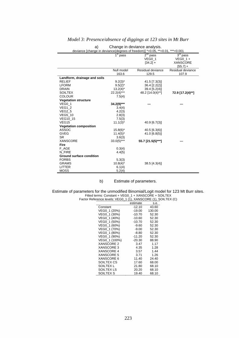
223

Model 3: Presence/absence of diggings at 123 sites in Mt Burr a) Change in deviance analysis.


2nd pass VEG0_1 [34.2] +

3rd pass VEG0_1 +

XANSCORE [55.7] +

Null model 163.6



Landform, drainage and soils RELIEF 9.2(3)* 41.5 [7.3(3)] LFORM 9.5(2)* 36.4 [2.2(2)] DRAIN 13.2(4)* 39.4 [5.2(4)] SOILTEX 22.2(4)*** 48.2 [14.0(4)**] 72.9 [17.2(4)**] COLOUR 7.5(4) Vegetation structure VEG0_1 34.2(9)*** --- --- VEG1_2 3.4(4) VEG2_5 4.2(3) VEG5_10 2.8(3) VEG10_15 7.5(3) VEG15 11.1(3)* 40.9 [6.7(3)] Vegetation composition ASSOC 15.8(6)* 40.5 [6.3(6)] GVEG 11.4(5)* 41.0 [6.8(5)] SR 3.6(3) XANSCORE 33.0(5)*** 55.7 [21.5(5)***] --- Fire F_AGE 0.3(4) N_FIRE 4.4(5) Ground surface condition FORBS 5.3(3) GRAMS 10.8(4)* 38.5 [4.3(4)] LITTER 6.1(4) MOSS 5.2(4)


Estimate of parameters for the unmodified Binomial/Logit model for 123 Mt Burr sites.

Fitted terms: Constant + VEG0_1 + XANSCORE + SOILTEX Factor Reference levels: VEG0_1 (1), XANSCORE (1), SOILTEX (C)

estimate s.e. Constant -12.10 43.60 VEG0_1 (20%) -19.00 130.00 VEG0_1 (30%) -10.70 52.30 VEG0_1 (40%) -10.60 52.30 VEG0_1 (50%) -10.70 52.30 VEG0_1 (60%) -9.60 52.30 VEG0_1 (70%) -9.00 52.30 VEG0_1 (80%) -8.80 52.30 VEG0_1 (90%) -11.20 52.30 VEG0_1 (100%) -20.30 88.90 XANSCORE 2 3.47 1.17 XANSCORE 3 4.35 1.28 XANSCORE 4 3.57 1.44 XANSCORE 5 3.71 1.26 XANSCORE 6 11.40 24.40 SOILTEX CS 17.60 68.00 SOILTEX L 21.80 68.10 SOILTEX LS 20.20 68.10 SOILTEX S 19.40 68.10

224

Model 4: Abundance of diggings at 123 sites in Mt Burr a) Change in deviance analysis.


2nd pass

XANSCORE [22.52] +

3rd pass XANSCORE +

SOILTEX [33.42] +

Null model 115.7



Landform, drainage and soils RELIEF 9.4(3)* 31.40 [8.88(3)]* 40.30 [6.88(3)] LFORM 16.2(2)** 27.08 [4.56(2)] DRAIN 14.2(4)** 28.81 [6.29(4)] SOILTEX 16.15(4)** 33.42 [10.9(4)*] --- COLOUR 6.0(4) Vegetation structure VEG0_1 19.65(9)* 34.42 [11.9(9)] VEG1_2 0.6(4) VEG2_5 2.8(3) VEG5_10 4.1(3) VEG10_15 3.6(3) VEG15 7.7(3) Vegetation composition ASSOC 12.1(6) GVEG 8.6(5) SR 6.9(3) XANSCORE 22.52(5)*** --- --- Fire F_AGE 0.3(4) N_FIRE 3.6(5) Ground surface condition FORBS 3.4(3) GRAMS 8.5(4) LITTER 5.6(4) MOSS 2.5(4)


Estimate of parameters for the unmodified Poisson/Log model for 123 Mt Burr sites. Fitted terms: Constant + XANSCORE + SOILTEX

Factor reference levels: XANSCORE (1), SOILTEX (C) estimate s.e. Constant -9.600 19.300 XANSCORE 2 1.700 0.604 XANSCORE 3 1.742 0.627 XANSCORE 4 1.653 0.688 XANSCORE 5 1.777 0.622 XANSCORE 6 2.183 0.667 SOILTEX CS 7.100 19.300 SOILTEX L 8.000 19.300 SOILTEX LS 7.700 19.300 SOILTEX S 7.900 19.300

Estimate of parameters for the modified Poisson/Log model for 123 Mt Burr sites. Fitted terms: Constant + XANSCORE + SOILTEX*

Factor reference levels: XANSCORE (1), SOILTEX* (CCSL) estimate s.e. Constant -2.343 0.609 Xanth_L 2 1.700 0.588 Xanth_L 3 1.704 0.609 Xanth_L 4 1.637 0.671 Xanth_L 5 1.793 0.608 Xanth_L 6 2.176 0.653 Soiltex_a LS 0.512 0.437 Soiltex_a S 0.708 0.302

225

Model 5: Presence/absence of diggings at 170 sites in Young a) Change in deviance analysis.


2nd pass ASSOC [34.5] +

3rd pass ASSOC+

VEG10_15 [46.6] +

4th pass ASSOC +

VEG10_15 + F_AGE [59.5] +

Null model 234.8




Landform, drainage and soils RELIEF 5.4(2) LFORM 14.6(2)*** 35.1 [0.6(2)] DRAIN 23.4(4)*** 35.1 [0.6(4)] SOILTEX 23.6(4)*** 38.3 [3.8(4)] COLOUR 23.1(4)*** 44.8 [10.3(4)*] 55.5 [8.9(4)] Vegetation structure VEG0_1 32.6(9)*** 51.1 [16.6(9)] VEG1_2 14.8(4)** 38.5 [4.0(4)] VEG2_5 1.5(3) VEG5_10 11.1(3)* 36.8 [2.3(3)] VEG10_15 14.3(3)** 46.6 [12.1(3)**] --- --- VEG15 7.1(3) Vegetation composition ASSOC 34.5(6)*** --- --- --- GVEG 22.7(5)*** 36.6 [2.1(5)] SR 22.4(3)*** 37.5 [3.0(3)] XANSCORE 28.2(5)*** 46.1 [11.6(5)*] 56.5 [9.9(5)] Fire F_AGE 12.6(4)* 45.5 [11.0(4)*] 59.5 [12.9(4)*] --- N_FIRE 7.6(5) Ground surface condition FORBS 8.7(4) GRAMS 17.6(4)** 44.4 [9.9(4)*] 57.7 [11.1(4)*] 70.1 [10.6(4)*] LITTER 3.9(4) MOSS 1.4(4)


Estimate of parameters for the unmodified Binomial/Logit model for 170 Young sites.

Fitted terms: Constant + ASSOC + VEG10_15 + F_AGE + GRAMS Factor reference levels: ASSOC (eucbax), VEG10_15 (<1%), F_AGE (0-4 years), GRAMS (<1%)

Estimate s.e. Constant -0.516 0.677 ASSOC eucobl 7.600 13.700 ASSOC eucova -1.279 0.719 ASSOC eucvim -0.520 1.010 ASSOC other 0.575 0.856 ASSOC reed/sedge -3.100 1.100 ASSOC shrubs -0.184 0.659 VEG10_15 (1-10%) 1.194 0.887 VEG10_15 (10-30%) 2.800 1.370 VEG10_15 (30-70%) -0.911 0.540 F_AGE (5-9 years) 2.119 0.844 F_ AGE (10-14 years) 2.529 0.931 F_ AGE (15-19 years) 1.101 0.772 F_ AGE (>19 years) 0.947 0.771 GRAMS (1-10%) -0.884 0.626 GRAMS (10-30%) -0.770 1.290 GRAMS (30-70%) -2.910 1.290 GRAMS (>70%) -2.290 1.400

226

Model 6: Abundance of diggings at 170 sites in Young a) Change in deviance analysis.


2nd pass ASSOC [32.9] +

3rd pass ASSOC + VEG10_15

[49.8] + Null model

182.3 Residual deviance

149.4 Residual deviance

132.5 Landform, drainage and soils RELIEF 2.9(3) LFORM 13.4(2)** 33.3 [0.4(2)] DRAIN 30.4(4)*** 40.1 [7.2(4)] SOILTEX 18.9(4)*** 37.2 [4.3(4)] COLOUR 18.8(4)*** 41.3 [8.4(4)] Vegetation structure VEG0_1 29.2(9)*** 46.5 [13.6(9)] VEG1_2 10.9(4)* 36.2 [3.3(4)] VEG2_5 1.5(3) VEG5_10 13.6(3)** 33.3[0.4(3)] VEG10_15 21.5(3)*** 49.8 [16.9(3)***] --- VEG15 5.6(3) Vegetation composition ASSOC 32.9(6)*** --- --- GVEG 18.6(5)** 39.2 [6.3(5)] SR 21.4(3)*** 37.3 [4.4(3)] XANSCORE 23.6(5)*** 40.1 [7.2(5)] Fire F_AGE 16.0(4)** 45.4 [12.5(4)*] 63.4 [13.6(4)**] N_FIRE 12.6(5)* 43.2 [10.3(5)] Ground surface condition FORBS 4.3(4) GRAMS 12.5(4)* 39.4 [6.5(4)] LITTER 3.1(4) MOSS 0.6(4)


Estimate of parameters for the unmodified Poisson/Log model for 344 sites. Fitted terms: Constant + ASSOC + VEG10_15 + F_AGE

Factor reference levels: ASSOC (eucbax), VEG10_15 (<1%), F_AGE (0-4 years) Estimate s.e. Constant -1.020 0.408 ASSOC eucobl 0.770 1.060 ASSOC eucova -0.737 0.396 ASSOC eucvim -0.594 0.618 ASSOC other 0.098 0.329 ASSOC reed/sedge -2.83 1.000 ASSOC shrubs -0.508 0.324 VEG10_15 (1-10%) 0.427 0.294 Vcov10_15 (10-30%) 0.694 0.250 Vcov10_15 (30-70%) -0.581 0.294 F_AGE (5-9 years) 1.149 0.423 F_AGE (10-14 years) 1.308 0.436 F_AGE (15-19 years) 0.798 0.441 F_AGE (>19 years) 0.835 0.444

Habitat Fragmentation and the Southern Brown Bandicoot

Documents

Transcript of Habitat Fragmentation and the Southern Brown Bandicoot