Habilitation Thesis Teza de Abilitare - UPT · Universitatea Politehnica Timişoara. Facultatea de...
145
Universitatea Politehnica Timişoara Facultatea de Electronică şi Telecomunicații Habilitation Thesis Teza de Abilitare GRAPHICAL PROGRAMMING IN MEDICINE, POWER ELECTRONICS AND MODERN EDUCATION PROGRAMARE GRAFICĂ ÎN MEDICINĂ, ELECTRONICĂ DE PUTERE ȘI TEHNICI EDUCAȚIONALE MODERNE Eng. MIHAELA RUXANDRA LASCU Professor, PhD 2016
Transcript of Habilitation Thesis Teza de Abilitare - UPT · Universitatea Politehnica Timişoara. Facultatea de...

Universitatea Politehnica Timişoara Facultatea de Electronică şi Telecomunicații
Habilitation Thesis Teza de Abilitare
GRAPHICAL PROGRAMMING IN MEDICINE, POWER ELECTRONICS AND MODERN EDUCATION
PROGRAMARE GRAFICĂ ÎN MEDICINĂ, ELECTRONICĂ DE PUTERE ȘI TEHNICI EDUCAȚIONALE MODERNE
Eng. MIHAELA RUXANDRA LASCU
Professor, PhD
2016

Mihaela Ruxandra Lascu Habilitation Thesis
2
TABLE OF CONTENTS
(a) Abstract 4
(b) Achievements and development plans 8
(c) Scientific, professional and academic achievements 14
1. Introduction 14
1.1 Main papers constituting the habilitation thesis 14
2. Finite element modeling in Electromagnetic Compatibility 15 2.1 The finite element method in shielding problems 15
2.1.1 Optimal magnetic shielding with grid structures 17 2.1.2 Geometrical models 20 2.1.3 Quickfield models results 22
2.2 Finite element method applied in modeling perturbations on printed circuit boards 27
2.2.1 Governing equations of two coupled lines 28 2.2.2 Capacitance and inductance matrix computation 30
2.3 Measurement Techniques for Determination of Shielding Effectiveness Characterizing Shielded Coaxial Cables 33 2.3.1 Measurement setup. Modified TEM measurement cell 33 2.3.2 TEMMC resonant frequency determination 36
3. Graphical programming in Biomedical Signal and Image Processing 43 3.1 Biomedical Signal Acquisition and Processing 43
3.1.1 Data Acquisition 43 3.1.2 LabVIEW for ECG maternal and fetal signal 51
3.2 Graphical programming in Event Detection using Pan –Tompkins Algorithm 57 3.2.1 Filtering for artifacts removal 58 3.2.2 The Pan Tompkins algorithm for QRS detection 64
3.3 Electrocardiogram Compression and Optimal ECG Filtering Algorithms 67 3.3.1 Neural networks for data compression 70 3.3.2 The Wiener filter 73 3.4 Electrocardiogram Event and Beat Detection 76 3.4.1 QRS detection using adaptive threshold 76 3.5 Real -Time 3D Echocardiography Processing 79 3.5.1 Three dimensional echocardiography processing 79 3.5.2 Image acquisition and processing methods 81 3.6 Feature Extraction in Digital Mammography 85 3.6.1 Mammography as digitized images 85 3.6.2 Image processing techniques 87 3.7 Compression, Noise Removal and Comparison in Digital Mammography 90

Mihaela Ruxandra Lascu Habilitation Thesis
3
3.7.1 Compression and noise removal 90 3.7.2 Image processing techniques 92 3.7.3 Mammography comparison 95 3.8 A Novel Morphological Image Segmentation with Application in 3D Echographic images 96 3.8.1 Morphological segmentation 97 3.8.2 Real time 3D image processing methodology 101
4. Graphical programming in Solar, Power Electronics and Modern Education 104 4.1 Solar radiation modeling, measurements and data processing 104 4.1.1 Experimental setup and database 106 4.1.2 Solar irradiation components 107 4.2 Transfer functions calculation in quasiresonant converters 108 4.2.1 Proposed state-space model 109 4.2.2 Transfer functions derivation 110 4.2.3 Verification and applications of the proposed method 112 4.3 E-learning Practical Teaching of Uncontrolled Rectifiers 116 4.3.1 Leonardo Da Vinci Project and its philosophy 117 4.3.2 Module and experiment description 121 4.4 Distance education in soft-switching inverters 125 4.4.1 System requirements and configuration 125 4.4.2 Description of the learning process 126
(d) Scientific, professional and academic future development plans 131
(e) References 136

Mihaela Ruxandra Lascu Habilitation Thesis
4
HABILITATION THESIS
(a) Abstract The present habilitation thesis summarizes my research activity after the PhD thesis was
defended in December 1998 at Politehnica University Timisoara. The PhD Thesis was certified by the Ministry of Education and Research, Order no. 3460 / 15. 03. 1999.
According to the regulations, the first part of this habilitation thesis is represented by the English and Romanian versions of the present abstract.
A description of the second part is given below. An overview of activity, stressing out the most important research, professional and
academic achievements: publications list and grants, new courses absorbed in the curricula and contributions to the academic curricula development, taught courses, diploma and dissertation adviser activity, invited professor, students internship, endowed laboratories and library, international cooperation, management activities, etc. The activity can be synthesized by the most important mentioned aspects that are a number of 69 research papers published in the above mentioned period, 23 research grants and 5 books.
In the following paragraphs a technical presentation regarding four main research topics is provided:
Electromagnetic compatibility - First a very powerful tool developed by the author for studying the magnetic field of shaped slotted screens is described. The proposed method is based on a circuital characterization of the structure, via the Finite Element Method (FEM) which is then combined with a modal expansion to compute the field inside and outside the border. The next chapter is concerned with predicting the electrical behavior of metallisation patterns printed onto dielectric substrates. It involves the generation of an equivalent circuit to model the electrical properties of the layout. This can be efficiently obtained and directly provided to a circuit simulation program. The last chapter presents a new test procedure for measuring the shielding effectiveness (SE) of shielded coaxial cables. The Transverse Electromagnetic (TEM) modified measurement cell with an asymmetrically placed conductor together with the proposed form of the cell, establish a quasi-uniform field in the zone where the testing cable is placed.
Graphical programming in biomedical signal and image processing - The first part of this chapter will describe a computer based signal acquisition, processing and analysis system using LabVIEW. Peak detection in electrocardiogram (ECG) is one of the solved problems using LabVIEW and filtering biomedical signals in different ways is a challenge that has to be solved. The next topic presented is graphical programming in event detection using Pan-Tompkins algorithm. QRS and ventricular beat detection is a basic procedure for electrocardiogram (ECG) processing and analysis. Further novel compression techniques are developed for portable heart-monitoring equipment that could also form the basis for more intelligent diagnostic systems thanks to the way the compression algorithms depend on signal classification. Then the design of an optimal Wiener filter is implemented to remove noise from a signal, assuming that the signal is statistically stationary and the noise is a stationary random process that is statistically signal independent. Two programs for compression and Wiener optimal filtering are developed in MATLAB. Also in this chapter a real-time QRS detection

Mihaela Ruxandra Lascu Habilitation Thesis
5
method implemented in LabVIEW is proposed, based on comparison between absolute values of summed differentiated electrocardiograms of one or more ECG leads and an adaptive threshold. Two algorithms were implemented in LabVIEW. In the last part a real-time 3D echocardiography and the corresponding algorithms that improve the quality of the image are presented. The second image application concerns the compression and noise removal of mammography images because these realize a preprocessing for the identification of microcalcification clusters in mammograms. A non-linear method is implemented in LabVIEW for performing image enhancement. The final chapter reviews ultrasound segmentation methods, in a broad sense, focusing on techniques developed for medical ultrasound images.
Solar Energy and Power Electronics - The first chapter introduces the first station in Romania (Eastern Europe) outfitted for systematic monitoring of solar irradiance on tilted surfaces. The resulted database is in many aspects unique for Romania, allowing for the first time to derive specific parameters, like diffuse fraction or sunshine number. The second chapter concerns Power Electronics. It is related to small signal transfer functions (control to output and audiosusceptibility) derivation in quasiresonant converters (QRCs). A matrix method based on state-space averaging of the PWM parent converter and switch cell conversion ratio is proposed. The result is general in the sense that the formalism is converter independent. The method was verified for all classical converters and perfect agreement with other tools was obtained.
E-learning techniques - The first part presents a comparison between classical hands-on laboratories and remote laboratories. Even they are very useful, hands-on laboratories have limitations regarding space, time and staff costs. These problems can be significantly alleviated by using remote experiments and remote laboratories when the students operate with real systems, although they are not present in the laboratory. The approach is based on constructivism and neoconstructivism concepts. The second part describes aspects regarding an E-learning approach of resonant ac inverters. The learning process is based on “Learning by Doing” paradigm supported by several learning tools: electronic course materials, interactive simulation, laboratory plants and real experiments accessed by Web Publishing Tools under LabVIEW.
The main results achieved in the field of Electromagnetic compatibility were published in 19 papers (17 as first author) and also 3 national grants tackled this field. Both 17 publications (16 as first author) and 3 national research grants refer to the field of graphical programming in biomedical signal and image processing. Solar energy and Power electronics is subjected to 13 papers (2 as first author) and 2 national grants, while E-learning teaching techniques have been investigated in 6 papers, 2 international grants and 2 national grants.
Scientific, professional and academic future development plans. Emphasis will fall both on wavelets in biomedical signal and image processing using graphical programming and on multimedia signal processing including 2D/3D image, video, speech, 2D/3D signal processing issues. Also wavelet transform and applications, time series analysis and stochastic processes will be of concern. As the first steps were already made, it is intended to consolidate the already established cooperation with researchers from “Victor Babeș” University of Medicine and Farmacy, Gastroenterology Department, regarding automated image analysis and diagnosis.
The third section is dedicated to the references.

Mihaela Ruxandra Lascu Habilitation Thesis
6
(a) Rezumat
Teza de abilitare prezintă pe scurt activitatea mea de cercetare, după ce teza de doctorat a fost prezentată în decembrie 1998, la Universitatea Politehnica din Timișoara. Teza de doctorat a fost confirmată de către Ministerul Educației și Cercetării prin Ordinul nr. 3460/15. 03. 1999.
În conformitate cu reglementările privind structura lucrării, prima parte a tezei de abilitare conține versiunile în limba engleză și limba română ale prezentului rezumat.
În cele de mai jos se face o descriere a celei de a doua secțiuni. O privire de ansamblu asupra activității, subliniind cele mai importante realizări din
cercetare, precum și a celor profesionale și academice: lista de publicații și granturi, cursuri noi introduse în planul de învățământ și contribuțiile la dezvoltarea planurilor de învățământ, cursuri predate, activitatea de conducere diplomă și disertație, profesor invitat, internship pentru studenți, laboratoare dotate și bibliotecă, cooperare internațională, activități de management, etc. Activitatea poate fi sintetizată prin cele mai importante aspecte menționate mai sus care sunt un număr de 69 de lucrări publicate în perioada menționată mai sus, 23 de granturi de cercetare și 5 cărți.
Prezentarea tehnică a patru direcții de cercetare abordate în această perioadă: Compatibilitatea electromagnetică - În prima parte am dezvoltat un instrument foarte
puternic de studiu a câmpului magnetic corespunzător unor ecrane cu fante. Metoda propusă se bazează pe o caracterizare de tip circuit a structurii prin metoda elementului finit (FEM), care este apoi combinată cu o reprezentare modală pentru a calcula câmpul în interiorul și exteriorul marginilor de frontieră. Următorul capitol se ocupă de estimarea comportamentului electric al modelelor de metalizare imprimate pe substraturi dielectrice. Aceasta implică generarea unui circuit echivalent pentru a modela proprietățile electrice ale plăcii cu circuite imprimate. Acest lucru este obținut în mod eficient și transmis direct la un program de simulare a circuitului. Ultimul capitol prezintă o nouă procedură de testare pentru măsurarea eficacității de ecranare (SE) pentru cablurile coaxiale ecranate. Celula de măsurare modificată Transverse Electromagnetic (TEM) cu un conductor asimetric plasat și forma propusă a celulei stabilesc în zona în care este plasat cablul de testare un câmp cvasi-uniform.
Programarea grafică în prelucrarea semnalelor și imaginilor biomedicale - În prima parte a acestui capitol se va descrie un sistem computerizat pentru achiziția, prelucrarea și analiza semnalelor cu ajutorul LabVIEW. Detecția de vârf în electrocardiogramă (ECG) este una din problemele ce au fost rezolvate de către autoare cu ajutorul LabVIEW. În schimb filtrarea semnalelor biomedicale în moduri diferite reprezintă o provocare care trebuie să fie rezolvată. Următoarea problemă prezentată, aparținând programării grafice, o reprezintă detectarea evenimentelor cu ajutorul algoritmului Pan-Tompkins. Detecția QRS-ului și bătăilor ventriculare sunt o procedură de bază pentru prelucrarea și analiza electrocardiogramei (ECG). În continuare, sunt dezvoltate noi tehnici de compresie pentru echipamentele portabile de monitorizare a inimii, care de asemenea pot constitui baza pentru sisteme de diagnosticare mai inteligente, datorită modului în care algoritmii de compresie depind de clasificarea semnalului. În următoarea etapă se proiectează unui filtru optimal Wiener care este implementat pentru a elimina zgomotul de la un semnal, având în vedere că semnalul este staționar statistic și zgomotul este un proces staționar aleator care este independent statistic de semnal. Sunt dezvoltate în MATLAB două programe de compresie și filtrare Wiener optimală. De asemenea, în acest capitol se propune o metodă de detectare în timp real a complexului QRS,

Mihaela Ruxandra Lascu Habilitation Thesis
7
implementată în LabVIEW, bazată pe comparația dintre valorile absolute ale electrocardiogramelor de la unul sau mai mulți electrozi ECG, însumate și derivate și un prag adaptiv. Au fost implementați în LabVIEW doi astfel de algoritmi. În ultima parte este prezentată o ecocardiografie 3D în timp real și algoritmii care îmbunătățesc calitatea imaginii prezentate. A doua aplicație referitoare la imagini se ocupă cu compresia și eliminarea zgomotului din imagini mamografice, deoarece aceste prelucrări reprezintă preprocesarea pentru identificarea formațiunilor de microcalcifiere din cadrul mamografiilor. Totodată este implementată o metodă neliniară pentru îmbunătățirea imaginilor. Ultima parte a capitolului face o trecere în revistă a metodelor de segmentare cu ultrasunete, într-un sens larg, concentrându-se pe tehnici dezvoltate pentru imagini medicale obținute pe baza ultrasunetelor.
Energie solară și electronică de putere - Primul capitol prezintă prima stație din România (Europa de Est), echipată pentru o monitorizare sistematică de iradiere solară pe suprafețe înclinate. Baza de date rezultată este unică pentru România, permițând pentru prima dată obținerea unor parametri specifici, cum ar fi fracțiunea difuză sau numărul solar. Al doilea capitol se referă la electronica de putere. El se referă la obținerea funcțiilor de transfer de semnal mic (control ieșire și audiosesceptibilitate) în convertoare cvasirezonante. Este propusă o metodă matricială bazată pe medierea în spatiul stărilor a convertorului PWM părinte și pe raportul de conversie al celulei de comutație. Rezultatul obținut este general în sensul că formalismul său nu depinde de convertorul analizat. Metoda a fost verificată pentru toate convertoarele clasice, constatându-se o coincidență perfectă cu rezultatele obținute prin alte tehnici.
Tehnici E-learning: În prima parte se prezintă laboratoarele hands-on clasice care sunt foarte utile, dar ele au limitări în ceea ce privește spațiul, timpul și costurile de personal. Aceste probleme pot fi micșorate în mod semnificativ prin utilizarea de experimente și laboratoare la distanță, atunci când studenții operează cu sisteme reale, deși aceștia nu sunt prezenți în laborator. Abordarea se face pe baza conceptelor de constructivism și neoconstructivism. Partea a doua descrie aspecte privind abordarea e-learning corespunzătoare unor invertoare de curent alternativ rezonante. Procesul de învățare se bazează pe “învățarea prin practică” paradigmă susținută de mai multe instrumente de învățare E-learning: materiale de curs electronice, simulare interactivă, instalații de laborator și experimente reale accesate prin Web Publishing Tools sub LabVIEW.
Principalele rezultate obținute în domeniul compatibilității electromagnetice au fost publicate în 19 lucrări (17 ca prim autor), și, de asemenea, 3 granturi naționale au abordat acest domeniu. Atât cele 17 publicații (16 ca prim autor) cât și cele 3 granturi naționale de cercetare se referă la domeniul programării grafice în prelucrarea semnalelor și imaginilor biomedicale. Energia solară și electronica de putere sunt reprezentate prin 13 lucrări științifice (2 ca prim autor) și 2 granturi naționale, în timp ce tehnicile de predare E-learning sunt dezvoltate în 6 lucrări științifice, 2 granturi internaționale și 2 granturi naționale.
Planuri științifice, profesionale și academice de dezvoltare în viitor. Accentul va cădea atât pe teoria undișoarelor aplicată în prelucrarea semnalelor și
imaginilor biomedicale cât și pe procesarea de imagini, inclusiv imagini 2D/3D, video, semnale de vorbire, prelucrarea semnalelor 2D/3D. De asemenea vor fi luate în considerare transformata wavelet si aplicatiile aferente transformatei precum și analiza seriilor de timp și a proceselor stohastice. Deoarece primii pași au fost deja făcuți, aceștia sunt destinați să consolideze cooperarea deja stabilită cu cercetatorii de la Universitatea de Medicină și Farmacie "Victor Babeș", Departamentul de Gastroenterologie, în ceea ce privește analiza automată și diagnostic.

Mihaela Ruxandra Lascu Habilitation Thesis
8
A treia secțiune este dedicată referințelor bibliografice.
(b) Achievements and development plans In December 1998 my PhD thesis “Contributions to ensure electromagnetic compatibility
in electronic equipment” was publicly defended at Politehnica University Timișoara. Therefore, the overview of activity will be made starting with January 1999.
I am going to present some of my main contributions and professional achievements for each research field:
1. Electromagnetic Compatibility First of all a very powerful tool for studying the magnetic field of shaped slotted screens
has been developed. The proposed method is based on a circuital characterization of the structure, via the Finite Element Method (FEM), which is then combined with a modal expansion to compute the field inside and outside the envelope. Although my analysis is focused in square slotted structures, the versatility of the Finite Element Method permits one to apply this method to any bidimensional envelope, no matter how many slots or dielectric parts it contains. It is also a review describing the basics of the finite-element method and its applications to EMI/C problems. It demonstrates how this method can help in the analysis of shield degradation in the presence of external conductors and electromagnetic leakage through slot configurations in a shielded enclosure. The development is given for an EMI application. The magnetic field inside and outside the slotted screens has been studied using the Finite Element Method. As a practical application, the magnetically performance of a slotted cylindrical and rectangular screen has been studied. In general, it is shown that coupling to the interior of slotted screens is maximized at frequencies corresponding to resonance of the shorted screen, provided that the fields do not vanish near the aperture.
The second part is concerned with predicting the electrical behavior of metallisation patterns printed onto dielectric substrates. The method described was initially aimed at the modeling of PCB layouts, but it is applicable to VLSI layouts, too. It involves the generation of an equivalent circuit to model the electrical properties of the layout. This can be efficiently obtained and directly provided to a circuit simulation program. Predictions can then be made of how the performance of a circuit implemented on a PCB is modified by its physical layout or of the performance of printed components such as spiral inductors.
The measurement of shielding effectiveness of coaxial cables is often limited by the dynamic range of the measurement system. The final part presents a new test procedure for measuring the shielding effectiveness (SE) of shielded coaxial cables. The Transverse Electromagnetic (TEM) modified measurement cell with an asymmetrically placed conductor together with the proposed form of the cell, establish a quasi-uniform field in the zone where the testing cable is placed. Moreover, the method operates over a broad frequency range with high accuracy.
Starting with 1998 I was member in following EMC research grants: Research Basis with multiple users for high voltage engineering and electromagnetic
compatibility, grant no.34/7004/1998-2002; Antenna calibration using auto-reciprocity method, grant no.28-3831/2000-2001; Electromagnetic Surveillance at County Hospital, grant no.32940/22.06.2004-2006.
Important papers published in this field are the following: LASCU MIHAELA RUXANDRA, The Finite Element Method In Shielding Problems
International Review of Electrical Engineering (I.R.E.E.) Vol.3, Nr.1, January-February 2008, pag.174-181.(ISI-Journal)

Mihaela Ruxandra Lascu Habilitation Thesis
9
LASCU MIHAELA RUXANDRA, Lascu Dan, Finite Element Method Applied in Modeling Perturbations on Printed Circuit Boards, International Review of Electrical Engineering (I.R.E.E.), Vol.3, Nr.2, March-April 2008, pp. 273-280. (ISI-Journal)
LASCU MIHAELA RUXANDRA, Measurement Techniques for Determination of Shielding Effectiveness Characterizing Shielded Coaxial Cables,The 11th International Conference on Optimization of Electrical and Electronic Equipment, Optim 2008, 22-24 May 2008, pp. 59-64.(ISI-Proceedings)
I have also teached the Electromagnetic Course and Laboratory (Bachelor level - IVth year Applied Electronics, Electronics and Telecommunication Faculty) at Politehnica University of Timișoara. Written books in this domain are: Aspects of electromagnetic compatibility in medicine, Waldpress Publishing House, ISBN 973-8453-65-8 (2005), Electromagnetic compatibility in medicine, Waldpress Publishing House, ISBN 973-36-0322-8, 2004.
2. Graphical programming in Biomedical Signal and Image Processing The reason in using graphical programming in this field is that this language is
the perfect environment in which to teach computer-based research skills. Moreover, with a minimum of difficulty, one could implement all sorts of sophisticated analysis techniques such as curve fitting, digital filtering, Fast Fourier transforming and of course signal and image processing. It is also possible to implement the wavelet transform and to study wavelets in medical imaging and tomography. Wavelet transforms have been applied to electrocardiogram signals for enhancing late potentials, reducing noise, QRS detection, normal and abnormal beat recognition. The methods used in graphical programming were conducted through continuous wavelet transform, multiresolution analysis and dyadic wavelet transform.
The first work will describe a computer based signal acquisition, processing and analysis system using LabVIEW, a graphical programming language for engineering applications. Biomedical signal acquisition has greatly advanced over the years, using many different technologies. E series multifunction data acquisition cards are used for the acquisition of biomedical signals together with the appropriate software NI-DAQ. With the increasing performance of the personal computer, computer based signal processing systems are becoming an efficient and cost-effective way of acquiring and analyzing these signals. The advanced analysis techniques available on the computer are becoming invaluable to the practicing physician. The diagnostic decision will be more accurate. Peak detection in electrocardiogram (ECG) is one of the solved problems using LabVIEW and filtering biomedical signals in different ways is a challenge that has to be solved.
The next topic presented is graphical programming in event detection using Pan-Tompkins algorithm. QRS and ventricular beat detection is a basic procedure for electrocardiogram (ECG) processing and analysis. A large variety of methods have been proposed and used, featuring high percentages of correct detection. Nevertheless, the problem remains open, especially with respect to higher detection accuracy in noisy ECGs.
I developed in LabVIEW the filtering for artifacts removal in biomedical signals and the Pan-Tompkins algorithm. I have investigated problems posed by artifact, noise and interference of various forms in the acquisition and analysis of several biomedical signals. We have also established links between the characteristics of certain events in a

Mihaela Ruxandra Lascu Habilitation Thesis
10
number of biomedical signals and the corresponding physiological or pathological events in the biomedical systems of concern. Event detection is an important step that is required before we may attempt to analyze the corresponding waves in more detail.
Further novel compression techniques are developed for portable heart-monitoring equipment that could also form the basis for more intelligent diagnostic systems thanks to the way the compression algorithms depend on signal classification. There are two main categories of compression which are employed for electrocardiogram signals: lossless and lossy.
In another work the design of an optimal Wiener filter is implemented to remove noise from a signal, considering that the signal is statistically stationary and the noise is a stationary random process that is statistically signal independent. Two programs for compression and Wiener optimal filtering are developed in MATLAB. Also in this chapter a real-time detection method implemented in LabVIEW is proposed, based on comparison between absolute values of summed differentiated electrocardiograms of one or more ECG leads and an adaptive threshold. The threshold combines three parameters: an adaptive slew-rate value, a second value which rises when high-frequency noise occurs and a third one intended to avoid the missing of low amplitude beats. Two algorithms were implemented in LabVIEW: The first algorithm detects the current beat, while the second algorithm measures the interval between two adjacent R peaks (R-R interval) and in addition performs a component analysis. The algorithms are self-adjusting to the thresholds and weighting constants, regardless of resolution and sampling frequency used. They operate with any number L of ECG leads, selfsynchronize to QRS or beat slopes and adapt to beat-to-beat intervals.
Finally bioimage processing is presented. First work contains a real-time 3D echocardiography and algorithms that improve the quality of the image. We provided a histogram, created line profiles, calculated measurement statistics associated with a region of interest in the image, produced a 3D real-time view and we adjusted the brightness, contrast and gamma of the acquired image. In the final part we implemented in LabVIEW the edge detection and the smoothing averaging.
The second image application concerns the compression and noise removal of mammography images as they implement a preprocessing for the identification of microcalcification clusters in mammograms. We proposed a general strategy for constructing algorithms and implementing them in LabVIEW for extracting microcalcifications clusters. A non-linear method is implemented in LabVIEW for performing image enhancement. The final chapter reviews ultrasound segmentation methods, in a broad sense, focusing on techniques developed for medical ultrasound images. Regarding the grants related to this field I have been director for: Modern Techniques in Processing and Hypermedia Transmission of Biomedical
Signals, Grant No.58GR/19.05.2006, Code CNCSIS 369/2007 Theme 19; Modern Techniques in Processing and Hypermedia Transmission of Biomedical
Signals, Grant No.58GR/19.05.2006, Code CNCSIS 369/2006 Theme 9. and member in: Hardware and software testing techniques for medical devices UPT 78/01.06.2004.
Important papers published in this field are the following:

Mihaela Ruxandra Lascu Habilitation Thesis
11
LASCU MIHAELA RUXANDRA, Dan Lascu, LabVIEW Based Biomedical Signal Acquisition and Processing, Proceedings of the 7th WSEAS International Conference on Signal, Speech and Image Processing, Beijing, China, 15-17 Septembrie 2007, pp. 38-43. (ISI-Proceeding)
LASCU MIHAELA RUXANDRA, Dan Lascu, LabVIEW Event Detection using Pan –Tompkins Algorithm, Proceedings of the 7th WSEAS International Conference on Signal, Speech and Image Processing, Beijing, China, 15-17 Septembrie 2007, pp. 32-37. (ISI-Proceeding)
LASCU MIHAELA RUXANDRA, Dan Lascu, Electrocardiogram Compression and Optimal Filtering Algorithm, Proceedings of the 7th WSEAS International Conference on Signal, Speech and Image Processing, Beijing, China, 15-17 Septembrie 2007, pp. 26-31. .(ISI-Proceeding)
LASCU MIHAELA RUXANDRA, Dan Lascu, Feature Extraction in Digital Mammography using LabVIEW, 2005 WSEAS International Conference on Dynamical Systems and Control, Venice, Italy, November 2-4, 2005, pp. 427-432, ISBN 960-8457-37-8.
LASCU MIHAELA RUXANDRA, Dan Lascu, Ioan Lie, Mihail Tănase, Compression, Noise Removal and Comparison in Digital Mammography using LabVIEW, Proceedings of the 10th WSEAS International Conference on COMPUTERS, Vouliagmeni, Athens, Greece, July 13-15, 2006, pp.671-676, ISSN:1790-5117, ISBN:960-8457-47-5. (Google Scholar)
LASCU MIHAELA RUXANDRA, Dan Lascu, Mammography using LabVIEW, WSEAS Transactions on Systems, Issue 4, Volume 5, April 2006, pp. 735-742, ISSN 1109-2777. (Scopus)
LASCU MIHAELA RUXANDRA, Lascu Dan, Tănase Mihail, Lie Ioan, Image Processing Techniques in Digital Mammography using LabVIEW, WSEAS Transactions on Circuits and Systems, Issue 7, Volume 5, pp. 887-894, August 2006, ISSN 1109-2734. (Scopus)
LASCU MIHAELA RUXANDRA, Lascu Dan, A New Morphological Image Segmentation with Application in 3D Echographic images, WSEAS Transactions on Electronics, Issue 3, Volume 4, pp. 72-82, 2008, ISSN 1109-9445. (Scopus)
LASCU MIHAELA RUXANDRA, Lascu Dan, Real-Time 3D Echocardiography Processing, Issue 4, Volume 5, pp. 142-154, ISSN 1109-9445. (Google Scholar)
I have introduced the Graphical Programming Course for Master studies, 1styear, Electronics and Telecommunication Faculty and the Virtual Instrumentation Course for bachelor, 3rd year, Electronics and Telecommunication Faculty. Both courses are programming courses at Politehnica University Timișoara.
Written books in this field are:
Advanced programming techniques in LabVIEW, Politehnica Publishing House Timișoara, ISBN: 978-973-625-532-8, 2007;
Flipping Book for practical activity at discipline Virtual Instrumentation (2013) - http://www.meo.etc.upt.ro/materii/laboratoare/IV/Documentatie%20IV.exe.
3. Solar Energy and Power Electronics The first work introduces the first station in Romania (Eastern Europe) outfitted
for systematic monitoring of solar irradiance on tilted surfaces. The resulted database is in many aspects unique for Romania, allowing for the first time to derive specific parameters, like diffuse fraction or sunshine number. Also for the first time, the data

Mihaela Ruxandra Lascu Habilitation Thesis
12
collected on tilted surfaces can be used to test models reported in literature and to recommend the most fitting for the region.
The second work concerns Power Electronics. It is related to small signal transfer functions (control to output and audiosusceptibility) derivation in quasiresonant converters (QRCs). State-space averaging is difficult to apply in QRCs because the linear ripple assumption is not valid for the state variables associated with the resonant elements. This handicap can be overpassed using the three terminal cell in which two out of the four variables are smooth. Consequently a matrix method based on state-space averaging of the PWM parent converter can still be applied with the duty cycle replaced by switch cell conversion ratio. The result is obtained in a close form being general in the sense that the formalism is converter independent. The method was verified for all classical converters and perfect agreement with other tools was obtained. The method can be applied to deriving the small signal transfer function for high order dc-dc converters such as: Cuk, Sepic or Zeta.
I have been member in following research grants related to this topic: Research project on the development and promotion of solar architecture solutions for
building integrated PV systems, PASOR project no.3-21039/2007, 2008, 2009, 2010. Optimization of hydro-electric generators through modernization of excitation systems
in order to increase energy efficiency and competitiveness, PNCDI2, contract no. 21040, 2008, 2009, 2010. Important papers published in this field are the following:
Paulescu Marius, Dughir Ciprian, Tulcan-Paulescu Eugenia, LASCU MIHAELA RUXANDRA, Paul Gravila, Traian Jurca, Solar radiation modeling and measurements in Timisoara, Romania: data and model quality, Environmental Engineering and Management Journal “Gheorghe Asachi” Technical University of Iasi, August 2010, Vol.9, No.8, pp. 1089-1095.(ISI Journal)
Jurca T, Paulescu E., Dughir C., LASCU MIHAELA RUXANDRA, Gavrila P., De Sabata A, Luminosu I, De Sabata C., Paulescu M Global Solar Irradiation Modeling and Measurement in Timisoara, Physics Conference (TIM), Timisoara, Romania, Nov 25-27, 2011, pp. 253-258, American Institute of Physics, Doi:10.1063/1.3647083. (ISI Proceedings)
LASCU MIHAELA RUXANDRA, A new method for calculating the transfer functions in quasiresonant converters, AECE Advances in Electrical and Computer Engineering, Vol.13, Issue 3, pp. 107-112, ISSN 1582-7445, e-ISSN 1844-7600, doi:10.4316/aece, Suceava 2013.(ISI Journal) I intend to continue research in the field concerning Renewable Energy.
4. E-learning techniques The first work stresses out the fact that even classical hands-on laboratories are
useful, they may have limitations regarding space, time and staff costs. These problems can be significantly alleviated by using remote experiments and remote laboratories where the students operate with real systems, although they are not present in the laboratory. The proliferation of web based distance education courses in recent years involves new challenges for teaching disciplines involving a high level of practical work.
The second work describes aspects regarding an E-learning approach of resonant ac inverters. The learning process is based on “Learning by Doing” paradigm supported

Mihaela Ruxandra Lascu Habilitation Thesis
13
by several learning tools: electronic course materials, interactive simulation, laboratory plants and real experiments accessed by Web Publishing Tools under LabVIEW. Built in LabVIEW and accompanied by a robust, flexible and versatile hardware, the experiment allows a comprehensive study by remote controlling and performing real measurements on the inverters. The study is offered in a gradual manner, according to the Leonardo da Vinci project EDIPE (E-learning Distance Interactive Practical Education) philosophy: theoretical aspects followed by simulations, while in the end the real experiments are investigated. Studying and experimenting access is opened for 24 hours a day, 7 days a week under the Moodle booking system.
I have been member in the international project Leonardo E-learning Distance Interactive Practical Education (EDIPE) CZ/06/B/PP-168022 - 2006, 2007, 2008, also an e-learning project.
I have participated as a member in:
DidaTec project (University School of initial and continuing training of teachers and trainers in the field of engineering and technical specialities) - code Contract: POSDRU/87/1.3/S/60891;
Concord (National Network of Teacher Continuing Education Pre-University Education Vocational and Technical) - code POSDRU/87/1.3/S/61397 project.
Both are e-learning projects for training, courses and mentoring.
Important papers published in this field are the following: Pavol Bauer, Lascu Dan, LASCU MIHAELA RUXANDRA, Popescu Viorel, Negoiţescu Dan,
Băbăiţă Mircea, Popovici Adrian, E-learning Practical Teaching of Uncontrolled Rectifiers, EPE 2009, 8-10 September, Barcelona, 13th European conference on Power Electronics and Applications, art.no.5278807, Vols 1-9, pp. 1840-1849, 2009. (ISI-Proceedings)
Lascu Dan, Bauer Pavol, Băbăiţă Mircea, LASCU MIHAELA RUXANDRA, Popescu Viorel, Popovici Adrian, Distance education in soft-switching inverters, Journal of Power Electronics, South Coreea, 2010, pp. 628-634. (ISI-journal)
I am teaching Virtual Instrumentation for the long-distance bachelor study program “Telecommunications Technologies and Systems”, 3rd year supported by the E-Learning Center of the Politehnica University Timișoara.
In this sense I wrote a Virtual Instrumentation course for e-learning students that was published at the Politehnica University Timişoara Printing House. (2008). For future research I would like to develop:
- Image-based modeling software for use in biomedical research; - Signal-based modeling software for use in biomedical research; - Advanced image processing in biology; - Wavelets in biomedical signal processing; - Graphical programming tools in green energy control and monitoring.
Finally, I would like to underline that I have an extensive experience as an engineer working in electronic and computer field, as a teacher and as a researcher.
Consequently, during the post PhD thesis period, my research activity and the results of the activities developed led to the discovery of certain algorithms concerning biosignal and bioimage processing, that have been implemented in the field of graphical programming.

Mihaela Ruxandra Lascu Habilitation Thesis
14
(c) Scientific, professional and academic achievements
1. INTRODUCTION
1.1 MAIN PAPERS CONSTITUTING THE HABILITATION THESIS
1. LASCU MIHAELA RUXANDRA, The Finite Element Method In Shielding Problems, International Review of Electrical Engineering (I.R.E.E.) Vol.3, Nr.1, January-February 2008, pp.174-181.
2. LASCU MIHAELA RUXANDRA, Lascu Dan, Finite Element Method Applied in Modeling Perturbations on Printed Circuit Boards, International Review of Electrical Engineering (I.R.E.E.), Vol.3, Nr.2, March-April 2008, pp.273-280.
3. LASCU MIHAELA RUXANDRA, Measurement Techniques for Determination of Shielding Effectiveness Characterizing Shielded Coaxial Cables, The 11th International Conference on Optimization of Electrical and Electronic Equipment, Optim 2008, 22-24 May 2008, pp.59-64.
4. LASCU MIHAELA RUXANDRA, Dan Lascu, LabVIEW Event Detection using Pan –Tompkins Algorithm, Proceedings of the 7th WSEAS International Conference on Signal, Speech and Image Processing, Beijing, China, 15-17 Septembrie 2007, pp. 32-37.
5. LASCU MIHAELA RUXANDRA, Dan Lascu, Electrocardiogram Compression and Optimal Filtering Algorithm, Proceedings of the 7th WSEAS International Conference on Signal, Speech and Image Processing, Beijing, China, 15-17 Septembrie 2007, pp. 26-31.
6. LASCU MIHAELA RUXANDRA, Lascu Dan, A New Morphological Image Segmentation with Application in 3D Echographic images, WSEAS Transactions on Electronics, Issue 3, Volume 4, pp 72-82, 2008, ISSN 1109-9445.
7. Paulescu Marius, Dughir Ciprian, Tulcan-Paulescu Eugenia, LASCU MIHAELA RUXANDRA, Paul Gravila, Traian Jurca, Solar radiation modeling and measurements in Timisoara, Romania: data and model quality, Environmental Engineering and Management Journal “Gheorghe Asachi” Technical University of Iasi, August 2010, Vol.9, No.8, pp.1089-1095.
8. LASCU MIHAELA RUXANDRA, A new method for calculating the transfer functions in quasiresonant converters, AECE Advances in Electrical and Computer Engineering, Vol.13, Issue 3, pp. 107-112,ISSN 1582-7445, e-ISSN 1844-7600, doi:10.4316/aece, Suceava 2013.
9. Pavol Bauer, Lascu Dan, LASCU MIHAELA RUXANDRA, Popescu Viorel, Negoiţescu Dan, Băbăiţă Mircea, Popovici Adrian, E-learning Practical Teaching of Uncontrolled Rectifiers, EPE 2009, 8-10 September, Barcelona, 13th European conference on Power Electronics and Applications, art.no.5278807, Vols 1-9, pp. 1840-1849, 2009.
10. Lascu Dan, Bauer Pavol, Băbăiţă Mircea, LASCU MIHAELA RUXANDRA, Popescu Viorel, Popovici Adrian, Distance education in soft-switching inverters, Journal of Power Electronics, South Coreea, 2010, pp.628-634.

Mihaela Ruxandra Lascu Habilitation Thesis
15
2. FINITE ELEMENT MODELING IN ELECTROMAGNETIC COMPATIBILITY
2.1 THE FINITE ELEMENT METHOD IN SHIELDING PROBLEMS
A very powerful tool for studying the magnetic field of shaped slotted screens has been developed [2.1-1], [2.1-2], [2.1-3]. The proposed method is based on a circuital characterization of the structure, via the Finite Element Method (FEM) [2.1-8], [2.1-9], [2.1-10], which is then combined with a modal expansion to compute the field inside and outside the border. Although my analysis is focused in square slotted structures [2.1-4], [2.1-5], [2.1-6] the versatility of the Finite Element Method permits one to apply this method to any bidimensional border no matter how many slots or dielectric parts it contains. This work is also a review describing the basics of the finite-element method and its applications to EMI/C problems. It demonstrates how this method can help in the analysis of shield degradation in the presence of external conductors and electromagnetic leakage through slot configurations in a shielded enclosure. The development is given for an EMI application related to shield degradation in the presence of external conductors [2.1-1], [2.1-7]. The magnetic field inside and outside the slotted screens has been studied using the Finite Element Method. As a practical application, the magnetically performance of a slotted cylindrical and rectangular screen has been studied. In general, it is shown that coupling to the interior of slotted screens is maximized at frequencies corresponding to resonance of the shorted screen, provided that the fields do not vanish near the aperture.
In complicated systems having more than one shielding surface, the process of coupling, penetration and propagation will be repeated until the component level is reached. This structured approach to viewing and analyzing complex systems permits division of the system into a number of simpler problems. It results in a sequence of analysis steps shown in an interaction sequence diagram, illustrating the flow of analysis and the models required for treating any specific system [2.1-12]. An example of such a diagram for external EMI sources acting on a system having a single shielding layer is indicated in Fig.2.1.1.
Fig.2.1.1 Interaction sequence diagram for a system with external excitation.
Not all EMC problems involve external sources of EMI. It is possible to have interference sources located within the system. For these cases the same topological concepts may be used,

Mihaela Ruxandra Lascu Habilitation Thesis
16
considering shielding layers located farther within the system as the primary barriers against the EMI.
Fig.2.1.2 illustrates an interaction sequence diagram suitable for internal sources. Note that in this figure, the possibility of having a direct or conducting connection between the source and the barrier is included.
Fig.2.1.2 Interaction sequence diagram for internal EMI sources.
Time-harmonic electromagnetic analysis is the study of electric and magnetic fields arising from the application of an alternating (AC) current source or an imposed alternating external field. Variation of the field with respect to time is assumed to be sinusoidal. All field components and electric currents vary with time according to the harmonic law:
,tcoszz z0 (2.1.1)
where z0 is a peak value of z, z its phase angle and - the angular frequency. The total current density in a conductor can be considered as a combination of a source current produced by the external voltage and an eddy current induced by the oscillating magnetic field
eddy0 jjj (2.1.2)
The problem is formulated as a partial differential equation for the complex amplitude of vector magnetic potential A (B=curl (A), B – magnetic flux density vector). The flux density is assumed to lie in the plane of model (xy or zr), while the vector of electric current density j and the vector potential A are orthogonal to it. Only jz and Az in planar case are not equal to zero. We will denote them simply j and A. The equation for planar case is
0xy
jgAiy
A1
yx
A1
x
(2.1.3)
where electric conductivity g and components of magnetic permeability tensor x and y are constants within each block of the model. Source current density j0 is assumed to be constant

Mihaela Ruxandra Lascu Habilitation Thesis
17
within each model block in planar case. The described formulas ignore displacement current
density term tD in the Ampere’s Law. Typically the displacement current density is not
significant until the operating frequency approaches the MHz range. In Fig.2.1.3 are presented three cases for three different frequencies concerning the penetration of the magnetic field inside the braided shield of a coaxial cable through a single aperture using the Finite Element Method [2.1.-8], [2.1-9].
The same manner the magnetic field penetrates through all the other apertures of the braided shield, because the cut-set in the braided shield is the same for all diamond or elliptic apertures. The study is performed at 50Hz, 5MHz and 5GHz. The model is characterized by the
following given parameters: air relative magnetic permeability =1, copper relative magnetic
permeability =1, copper conductivity =58.005.000 S/m, current in the conductor I=1A. It is possible to observe that by an increasing of frequency the strength H(A/m) is as well increasing, but the permeability and the flux density B(T) are decreasing. Making a comparison of the results obtained by different methods it is possible to see that they are similar. For example for values of the maximum flux density in Y-direction it is possible to obtain: ANSYS 0.42, COSMOS/M 0.404, QUICKFIELD 0.417 [2.1-11].
The compilation time needed for a high frequency is longer than the compilation time
for low frequencies. For example, by f=50Hz the needed time is 223s and by f=5GHz the needed
time is 1498s.
The complex impedance per unit length of the conductor can be obtained from the
equation IVZ where V is the voltage drop per length unit. This voltage drop on the
conductor can be obtained in Local Values mode of the postprocessing window, clicking an arbitrary point within the conductor. Comparison of results by f=50Hz are: ReZ(Ohm/m) by reference program ANSYS is 0.00017555 and with Quickfield the value is 0.00017550. For ImZ(Ohm/m) obtained by the reference is 0.00047113 and with Quickfield 0.00047111 [2.1-11].
2.1.1 OPTIMAL MAGNETIC SHIELDING WITH GRID STRUCTURES
In this work [2.1-13] the case with an external conductor placed near an aperture located on a shield is investigated. The quantity of energy is increasing very much when a coupling is borne due to the existence of this slot. The papers in the literature [2.1-1], [2.1-5] refer only to small geometries compared to the wavelength and to studies that specify the Finite Difference Method. The problem will be solved using the Finite Element Method (FEM) and the provided solutions can be used for much larger geometries. Generally, the discontinuities of the shield have a more pronounced effect on the dispersion of the magnetic field than on the dispersion of the electric field. The shielding of an electrical disturbance source from a potential receiver is a powerful technique in EMC control. Shields can be as large and rigid as whole steel lined buildings to test military equipment, to test shield sensitive computer systems or as small and flexible as the braids on coaxial cables. The understanding of the principles involved however is not entirely obvious, except in a few idealized cases, where the use of a particular approximation is justified. It is always possible in principle to solve Maxwell’s equations with the appropriate boundary conditions to obtain an accurate solution. Analytical solutions can only be obtained for a few idealized shapes (spherical, cylindrical, grid shells, etc.) composed of known homogeneous materials excited by a well defined field.

Mihaela Ruxandra Lascu Habilitation Thesis
18
Fig.2.1.3. Comparison between three different frequencies cases concerning the
penetration of the magnetic field inside the shield of a coaxial cable through a single
aperture.
The range of shapes can be extended using numerical techniques [2.1-9] but the solution for any engineering shield composed of real materials, its associated jointing and excited by an
0.00000.08180.16360.24540.32720.40900.49080.57260.65440.73620.8180
RMSH( A/m)Strength
0.0000.0830.1660.2490.3320.4150.4980.5810.6640.7470.830
RMSH( A/m)Strength
0.0000.5091.0181.5272.0362.5453.0543.5634.0724.5815.090
RMSH( 10-3 A/m)Strength
Time Harmonic Magnetics;
Analyses of Strength H(A/m);
Frequency = 50Hz;
Total compilation time=223s;
Copper shield with diamond shaped
aperture or ellipse aperture;
Total current = 1 A through the
conductor placed in the middle of
the shield.
Time Harmonic Magnetics;
Analyses of Strength H(A/m);
Frequency = 5MHz;
Total compilation time=486s;
Copper shield with diamond shaped
aperture or ellipse aperture;
Total current = 1 A through the conductor placed in the middle of the shield.
Time Harmonic Magnetics;
Analyses of Strength H(A/m);
Frequency = 5GHz;
Total compilation time=1498s;
Copper shield with diamond shaped aperture or ellipse
aperture;
Total current = 1 A through the conductor placed in the
middle of the shield.
Mihaela Ruxandra Lascu Habilitation Thesis
19
arbitrary source having non-ideal characteristics is currently prohibitively expensive in computer requirements.
0.000
0.194
0.388
0.582
0.776
0.970
1.164
1.358
1.552
1.746
1.940
B( 10-3
T)
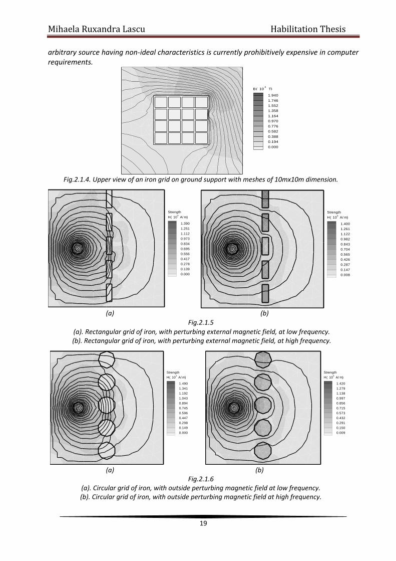
Fig.2.1.4. Upper view of an iron grid on ground support with meshes of 10mx10m dimension.
(a) (b)
Fig.2.1.5
(a). Rectangular grid of iron, with perturbing external magnetic field, at low frequency. (b). Rectangular grid of iron, with perturbing external magnetic field, at high frequency.
(a) (b)
Fig.2.1.6 (a). Circular grid of iron, with outside perturbing magnetic field at low frequency. (b). Circular grid of iron, with outside perturbing magnetic field at high frequency.
0.000
0.139
0.278
0.417
0.556
0.695
0.834
0.973
1.112
1.251
1.390
H( 104
A/ m)
Strength
0.008
0.147
0.287
0.426
0.565
0.704
0.843
0.982
1.122
1.261
1.400
H( 106
A/ m)
Strength
0.000
0.149
0.298
0.447
0.596
0.745
0.894
1.043
1.192
1.341
1.490
H( 104
A/ m)
Strength
0.009
0.150
0.291
0.432
0.573
0.715
0.856
0.997
1.138
1.279
1.420
H( 106
A/ m)
Strength

Mihaela Ruxandra Lascu Habilitation Thesis
20
In Fig.2.1.4 is presented an up-side view of a shielding in grid structure. The shield is made of iron. The meshes of the grid have a dimension of 10mx10m. The perturbing magnetic field source has a normal incidence about the structure. The structure is represented on the following dimensions: xє[-50,50]m and yє[0,100]m. In all situations concerning the grids we have to take into account the symmetry and repetition principle [2.1-2]. In Fig.2.1.5 (a) is illustrated a rectangular iron grid in section, with outside perturbing magnetic field, at low frequencies. In comparison, in Fig.2.1.5 (b) is represented the same value of the magnetic field strength in the protected space from the protected right side of the grid, in monitoring point x=60, y=55. At high frequencies, compared to the low frequencies the value of the magnetic field strength is much higher. This aspect leads to a diminution of the shielding effectiveness, as well as to a diminution of the permeability of the material that realize the grid. In a similar way, we studied in Fig.2.1.6 the grid shielding with circular section. The conclusions obtained in this situation are similar to that obtained in the above presented situation. In Table 2.1.1 are comparatively presented the values of the shielding effectiveness for the two types of the presented grid shields at low and high frequencies.
TABLE 2.1.1
Shielding Effectiveness for a Grid Structure
Grid Type Low Frequency (50Hz) SE[dB]
High Frequency (10MHz) SE[dB]
Circular grid 19.97 14.98
Rectangular grid 20.37 16
It is for this reason that the various approximations are so important both in obtaining an estimate of a particular shielding effectiveness and in building up a physical picture of how the shield acts. The physical picture enables a designer to deviate more safely from published design tables for homogeneous shields [2.1-4] when involved in the development of a specific practical shield. Evaluating the previous pictures and Table 2.1.1 it is possible to observe that it is better to use a rectangular grid in place of a circular grid. This choice is made because the shielding effectiveness with this type of grid is better than the one obtained with the other type. At both types of grids it is possible to observe a diminution of the shielding effectiveness at high frequencies. Analyzing the numerical results it may be observed that obvious emissions (a high rising H, in the monitoring point) all around the resonance frequency of each structure. The radiation phenomenon at low frequencies is easy to observe as well. The larger the meshes of the structure are the easier is to observe the radiation phenomenon. That is why it is necessary to diminish the meshes of the structure, for reducing the undesired radiations. In conclusion, it is possible to say that the programs developed for testing and verifying different types of grids may be used with different material properties and different perturbation sources.
2.1.2 GEOMETRICAL MODELS
All the cases studied in this paragraph use the same basic geometric model. An external source is localized under a shield and an external conductor is localized upside. Some monitoring points are placed above the external conductor in form of an arc of a circle. For all the models we shall use the same shield-aperture structure.
Mihaela Ruxandra Lascu Habilitation Thesis
21
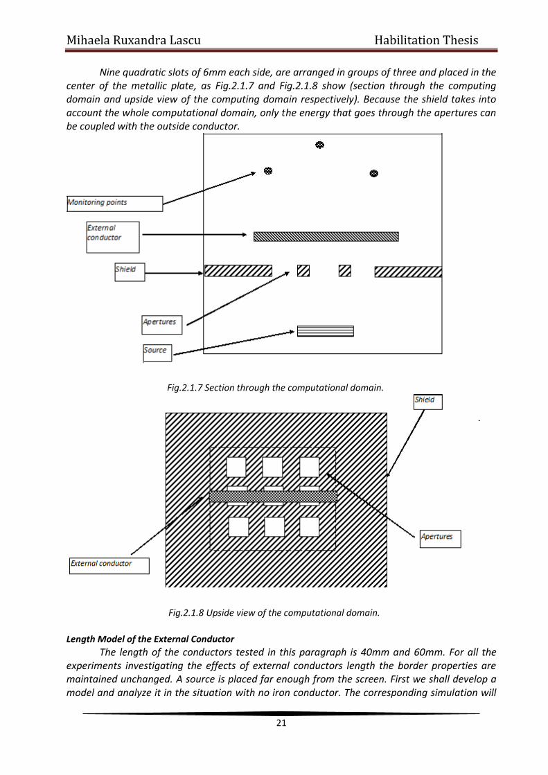
Nine quadratic slots of 6mm each side, are arranged in groups of three and placed in the center of the metallic plate, as Fig.2.1.7 and Fig.2.1.8 show (section through the computing domain and upside view of the computing domain respectively). Because the shield takes into account the whole computational domain, only the energy that goes through the apertures can be coupled with the outside conductor.
Fig.2.1.7 Section through the computational domain.
Fig.2.1.8 Upside view of the computational domain.
Length Model of the External Conductor
The length of the conductors tested in this paragraph is 40mm and 60mm. For all the experiments investigating the effects of external conductors length the border properties are maintained unchanged. A source is placed far enough from the screen. First we shall develop a model and analyze it in the situation with no iron conductor. The corresponding simulation will

Mihaela Ruxandra Lascu Habilitation Thesis
22
be the reference simulation for the cases in which iron and copper conductors of different lengths will be examined. Coupling Model of the Source When the source is placed near the shield it is not possible to ignore the direct coupling that occurs. I simulated two positions for the source: far from the shield and close to the shield. For each position the simulations will be executed with and without the presence of a conductor.
2.1.3 QUICKFIELD MODELS RESULTS
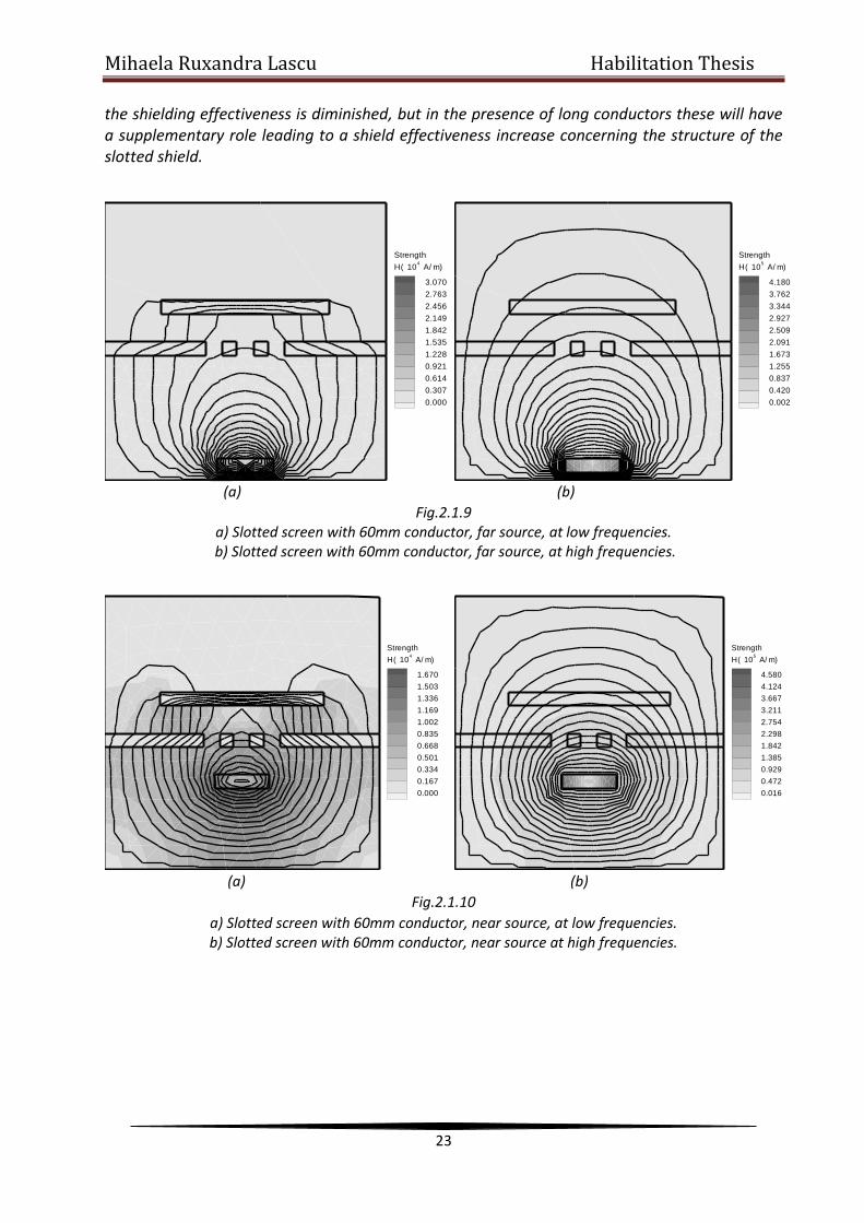
We focus on the magnetic field strength in the monitoring points for the previous presented situations. The number of points is minimized for obtaining only the peaks of the emission levels. At the same time, we determine the magnetic field strength variation in the three monitoring points with the following coordinates: MON1(25,80), MON2(50,95), MON3(75,80). It has to be considered the greatest value obtained in one of these points and after this it will be possible to calculate the corresponding shielding effectiveness of the slotted shield. The FEM model [2.1-10], [2.1-11] corresponding to the above presented structure is illustrated in Fig.2.1.9. At low frequencies (for ex.50Hz) the conductor is made of iron. At high frequencies (for ex. 1MHz) the conductor can be of any material. Current does not pass the conductor. In this situation the conductor has supplementary attenuation effect. Practically it contributes to the increasing of the shielding effectiveness. This can also be observed with the help of Table 2.1.2, when the conductor is directly placed upon the slots. We continue the study in Fig.2.1.10 with the analysis of the previous structure, in which we consider a near placed source. Examining the obtained results for H in the monitoring points from the protected space, it is possible to observe that these values are much higher than the values obtained in the previous situation. This situation is due to the position of the source, which in this position is nearer to the slotted screen, than in the previous situation. We find a diminution of the shielding effectiveness compared to the situation of the previous model. In Table 2.1.2 these low values of diminished shielding effectiveness are mentioned.
The models illustrated in Fig.2.1.11 refer to the initial situation. For Fig.2.1.7 only in this example the length of the conductor will be not so long as in the already investigated cases. This conductor structure will lead to a diminution of the shielding effectiveness for both low and high frequencies. Table 2.1.2 shows the values of the shielding effectiveness in this situation. Comparing to the situations without conductor, that is considered the reference model, it is possible to observe that in this case when conductors are used, the shielding effectiveness is growing. In Fig.2.1.12 is presented a particular case at high frequency in which the source and the conductor in which the current can flow in two directions are considered to be copper made and they are placed at the same distance with respect to the slotted shield. Evaluating the model in Fig.2.1.12 with the help of FEM [2.1-9], [2.1-10] it is established that in the conductor the field is approximately zero. The two opposite currents that are flowing through the source and the conductor are creating opposite directions fields, which are leading to a near zero field in the zone of the conductor. In this work FEM models [2.1-10], [2.1-11] for slotted shields in the presence of external conductors are developed. The behavior is analyzed in different circumstances met in practice and as a conclusion it is possible to say that at high frequencies
Mihaela Ruxandra Lascu Habilitation Thesis
23
the shielding effectiveness is diminished, but in the presence of long conductors these will have a supplementary role leading to a shield effectiveness increase concerning the structure of the slotted shield.
(a) (b)
Fig.2.1.9 a) Slotted screen with 60mm conductor, far source, at low frequencies.
b) Slotted screen with 60mm conductor, far source, at high frequencies.
(a) (b)
Fig.2.1.10
a) Slotted screen with 60mm conductor, near source, at low frequencies. b) Slotted screen with 60mm conductor, near source at high frequencies.
0.000
0.307
0.614
0.921
1.228
1.535
1.842
2.149
2.456
2.763
3.070
H( 104
A/ m)
Strength
0.002
0.420
0.837
1.255
1.673
2.091
2.509
2.927
3.344
3.762
4.180
H( 105
A/ m)
Strength
0.000
0.167
0.334
0.501
0.668
0.835
1.002
1.169
1.336
1.503
1.670
H( 104
A/ m)
Strength
0.016
0.472
0.929
1.385
1.842
2.298
2.754
3.211
3.667
4.124
4.580
H( 105
A/ m)
Strength

Mihaela Ruxandra Lascu Habilitation Thesis
24
(a) (b)
Fig.2.1.11 a) Slotted screen with 40mm conductor, near source, at low frequencies.
b) Slotted screen with 40mm conductor, near source, at high frequencies.
Fig.2.1.12 Slotted screen with the conductor and the source placed at equal distance to the shield.
Table 2.1.2 The Shielding Effectivness Characterizing Slotted Screens
Source position Cond. length
SE[dB] LF
SE[dB] HF
Source position Cond. length
SE[dB] LF
SE[dB] HF
Source position Cond. length
SE[dB] LF
SE[dB] HF
Without Cond.
Cond. 60mm
Cond. 40mm
Far source
41.13 35.5 Far source
52 45.89 Far source
46.03 45.82
Near source
17.90 16.66 Near source
28.96 26.94 Near source
23.25 22.95
FEM ANALYSIS OF A DOUBLE-LAYERED CYLINDRICAL STRUCTURE In Fig. 2.1.13 FEM analysis for a double-layered cylindrical structure with a single slot is presented. The study is performed for low and high frequencies. The values for B and H that appear in the considered monitored side of the shield, where the slot is placed, are much higher than the values obtained on the side, where no slot is present. As the frequency is increasing it is
0.000
0.306
0.612
0.918
1.224
1.530
1.836
2.142
2.448
2.754
3.060
H( 104
A/ m)
Strength
0.002
0.419
0.836
1.252
1.669
2.086
2.503
2.920
3.336
3.753
4.170
H( 105
A/ m)
Strength
0.000
0.498
0.996
1.494
1.992
2.490
2.988
3.486
3.984
4.482
4.980
H( 105
A/ m)
Strength

Mihaela Ruxandra Lascu Habilitation Thesis
25
possible to see that the values of B and H in the monitoring point are getting higher. Therefore, due to the slot, the shielding effectiveness is considerable affected. On the other side diminution is caused also by the increase of the frequency. Due to the raising of frequency the permeability of the screen diminishes, which is possible to be observed in Fig.2.1.6 b) by the increasing of the magnetic field strength in the copper layer. In Fig. 2.1.14 is presented an identical shield to the previous one, except for the fact the shield has four slots. The values of B and H increase very much compared to the previous situation. Because of the increased number of slots and because of the frequency increase the shielding effectiveness falls considerable compared to the previous situation. In Fig.2.1.15 is illustrated an identical model to the previous one, but with the four symmetrically placed slots replaced by a global slot. It is established that the obtained values in this situation are higher than the ones obtained in the previous situation. As a conclusion, we may state that it is preferable to use four symmetrically displaced little slots. The values for the SE are presented in Table 2.1.3. It has been shown that shielding theories are in good agreement with the experiments provided the field geometries are essentially solutions of Maxwell’s equations for specific boundary conditions. The solutions usually have a restricted range of applicability.
(a) (b)
Fig.2.1.13 a) Double layered cylindrical shield outside Fe – inside Cu with one slot, at low frequencies. b) Double layered cylindrical shield outside Fe – inside Cu with one slot, at high frequencies.
(a) (b)
Fig.2.1.14
a) Double layered cylindrical shield outside Fe – inside Cu with four slots, at low frequencies. b) Double layered cylindrical shield outside Fe – inside Cu with four slots, at high frequencies.
0.001
0.538
1.075
1.612
2.149
2.686
3.222
3.759
4.296
4.833
5.370
H( 104
A/ m)
Strength
0.000
0.544
1.087
1.630
2.173
2.715
3.258
3.801
4.344
4.887
5.430
H( 105
A/ m)
Strength
0.002
0.160
0.317
0.475
0.633
0.791
0.949
1.107
1.264
1.422
1.580
H( 104
A/ m)
Strength
0.001
0.155
0.309
0.463
0.617
0.771
0.925
1.078
1.232
1.386
1.540
H( 105
A/ m)
Strength

Mihaela Ruxandra Lascu Habilitation Thesis
26
(a) (b)
Fig.2.1.15
a) Double layered cylindrical shield outside Fe – inside Cu with one slot equivalent to four slots, at low frequencies. b) Double layered cylindrical shield outside Fe – inside Cu with one slot equivalent to four slots, at high frequencies.
0
5
10
15
20
1 10 100 1000 110
SE [dB]
f [MHz]
FEM analysis
experiment
Fig.2.1.16 Shielding effectiveness against frequency (FEM analysis and experiment).
Table 2.1.3 Shielding effectiveness values for a cylindrical and rectangular shield with two layers, inside layer copper, outside layer iron, in the monitoring point, where H has the highest value.
Nr. of slots SE[dB] measured
No slot 1 slot LF
1 slot HF
4 slots LF
4 slots LF
Equiv. 4 slots LF
Equiv. 4 slots HF
Cylindrical shield
15.56 ≈6 1.375 1.333 1.119 1.101 1.111 1.099
Rectangular shield
13.97 ≈5 1.333 1.125 1.14 1.03 1 1
In conclusion, SE profile in the (1÷1000 MHz) domain is represented in Fig.2.1.16. In this work FEM simulations of laminated double-layered cylindrical and rectangular shields with slots
0.000
0.213
0.426
0.639
0.852
1.065
1.278
1.491
1.704
1.917
2.130
H( 104
A/ m)
Strength
0.000
0.423
0.845
1.267
1.689
2.110
2.532
2.954
3.376
3.798
4.220
H( 105
A/ m)
Strength

Mihaela Ruxandra Lascu Habilitation Thesis
27
are performed. As well a comparison between the experimental results [2.1-6], [2.1-9] is made and it is demonstrated that the resulting values obtained by the FEM method have a deviation of maximum 4 dB compared to the measured values. Finally, it should be emphasized in principle that an isolated perfect shield that surrounds a protected system does not require earthing. The potential of the shield may take any value without affecting the inside circuits. However, real shields exhibit apertures and are connected to cables (signal, mains, etc.) so that unless the shield is earthed noise voltages on the shield can couple to the interior circuits. The safety requirements for mains connection will also require an earthing.
2.2 FINITE ELEMENT METHOD APPLIED IN MODELING PERTURBATIONS ON PRINTED CIRCUIT BOARDS
This work is concerned with predicting the electrical behavior of metallisation patterns
printed onto dielectric substrates. The method described was initially aimed at the modeling of PCB layouts, but is also applicable to VLSI layouts. It involves the generation of an equivalent circuit to model the electrical properties of the layout. This can be efficiently obtained and directly provided to a circuit simulation program. Predictions can then be made of how the performance of a circuit implemented on a PCB [2.2-1] is modified by its physical layout or by the presence of printed components such as spiral inductors. However, as circuit design became more complex and constraints on space increased, problems began to be seen, particularly in high-frequency design [2.2-3], [2.2-5]. The cause of these was that in fact the PCB behaves in a complex manner, with various electrical-loss and internal-coupling mechanisms. Electromagnetic modeling has a long history: some of the basic techniques were developed more than a century ago, by Maxwell and others [2.2-7]. However, before the widespread use of computers, only a very limited range of problems could be tackled, such as isolated conducting objects of symmetrical shape. The development of digital computers changed all that. There is now a large set of numerical techniques that can be applied and a vast associated literature describing methods and particular applications. All of the methods work by transforming the continuum set of integral-differential equations into a set of purely algebraic equations that can be solved on a computer using standard numerical techniques. For electromagnetic modeling, there is a fairly natural subdivision of the techniques into differential and integral methods. The problem of two coupling transmission lines (TL) is essential in the design of PCB and VLSI. The basic definitions of capacitance and inductance are explained and used as the starting point for a detailed analysis which demonstrates that the equivalent-circuit model for the PCB provides an approximate solution to Maxwell’s equations [2.2-7]. The main approximations are:
the assumption that the dominant coupling effects take place over electrically short distances, and
the types of charge and current distribution assumed in the conductors. Both of these approximations are well founded for the application areas envisaged, namely electrically small but geometrically complex structures, and their validity is borne out by accuracy of the results obtained.

Mihaela Ruxandra Lascu Habilitation Thesis
28
The aim of this analysis is to produce an equivalent-circuit model for the PCB [2.2-1], [2.2-2], [2.2-3], [2.2-4]. The current flow in the inductors and the charge in the capacitors provide an approximation of the real charge and current distributions, while the resistors represent both dielectric and resistive losses [2.2-5], [2.2-6], [2.2-7].
2.2.1 GOVERNING EQUATIONS OF TWO COUPLED LINES
The equivalent circuit model of a part dx belonging to two lossless TL, coupled, with common returning is represented in Fig.2.2.1. It is necessary to take into account the mutual inductivity that appears between line 1 and the ground, as well as that is appearing between line 2 and the ground.
According to the presented figure, we may write the following relationships:
t
iL
t
iL
t
iL
x
u 010
212
111
1
∂
∂
∂
∂
∂
∂ (2.2.1)
t
iL
t
iL
t
iL
x
u
0
20
2
22
1
21
2
∂
∂
∂
∂
∂
∂ (2.2.2)
t
uC
t
u)CCC(
x
i
∂
∂
∂
∂
∂
∂2
12
1
101211
1 (2.2.3)
t
u)CCC(
t
uC
x
i
∂
∂
∂
∂
∂
∂ 2
201222
1
12
2 (2.2.4)
it
Lux ∂
∂
∂
∂ (2.2.5)
ut
Cix ∂
∂
∂
∂ (2.2.6)
Cpdx C1dx
C2dx
L1dx
L2dx
Mdx
i1
u1
u2
i2
i1+di1
i2+di2
(0V)
x x+dx
x
u1+du1
u2+du2
i0 L0dx
Fig.2.2.1. Equivalent circuit model of a part dx belonging to two TL, lossless, coupled, with common returning.
The previous relationships (2.2.1)(2.2.4) can be rewritten in matrix form as in (2.2.5) and (2.2.6). The derivatives with respect to x of (2.2.5) and (2.2.6) replaced in the upper equations, lead to:
CLAut
CLux
u2
2
2
2
∂
∂
∂
∂ (2.2.7)
LCAit
LCix
i2
2
2
2
∂
∂
∂
∂ (2.2.8)

Mihaela Ruxandra Lascu Habilitation Thesis
29
where
pp
pp
t
t
CCC
CCCC
;LM
MLL;
i
ii;
u
uu
2
1
2
1
In the previous relationships L11, C11 represent the line parameters of line 1 in the presence of line 2 and L12(L21), C12(C21) the coupling parameters between the two lines – the mutual line inductance and the line parasitic capacitance. In case of lossless symmetrical, with common returning lines it is known that:
ppppppp
t
CCCCCCCCCCCCCC
MMMMMLMLMLLLLL
212020101021122211
2122011021122211
Equations (2.2.1) and (2.2.2) are showing the parasitic phenomenon – the undesirable energy transfer between one circuit and the other. Thus in (2.2.1) the voltage u1 depends on the current i2 in the other line. Similarly, u2 depends on i1, and so on. Line 1 couples in a parasitic way line 2, but line 2 couples in a parasitic way line 1 as well. Equations (2.2.7), (2.2.8) are putting in evidence the coupling: the voltage u1 depends as well on voltage u2, and so on – the result is not a set of second order differential equations in the expressions of u1 and u2 like in the study of isolated lines. To solve the problem it is necessary solving the systems (2.2.7) and (2.2.8) conditioned
by the equations (2.2.1)(2.2.4). The method used in this work is the finite-element method (FEM) [2.2-8], [2.2-9],
[2.2-10]. FEM is a more recent development than the finite-difference method. It was initially developed in the field of structural analysis and as a result much of the literature on it involves mechanical and civil engineering. The essence of the method is the development of an approximation of the field vectors over the entire domain, rather than approximating the governing equations at a finite set of points as in the finite-difference method. This is done by subdividing the entire region into a set of elements (usually triangles or quadrilaterals for a two-dimensional region) and defining a set of basis functions (or trial functions) to represent the fields variation within each element. The field Ex for example is then represented by
N
iiix rψξrE
1
(2.2.9)
where i is a set of N basis functions, with unknown coefficients i. A set of equations to determine the unknown coefficients is generated either by a variational approach or by the use of weighting functions that effectively produce samples of the approximate solution, the governing equation and the boundary conditions. The resulting
solution, which contains the set of coefficients i is an approximation for the true fields over the entire domain. The problems of interest in PCB have the following properties [2.2-12], [2.2-17]:
the dielectric materials used for substrates can be assumed to be arranged in a layered structure, with each layer having constant, isotropic material properties.
the arrangement of conductors can be extremely complex, but nearly all are in a plane parallel to the substrate interfaces.

Mihaela Ruxandra Lascu Habilitation Thesis
30
the applications are usually electrically small, or else all significant electromagnetic coupling occur over electrically small distances.
the applications are often unbounded.
the results of the simulation have to be made available to circuit designers as circuit theory parameters [2.2-13]. A typical configuration is represented in Fig. 2.2.2 and Fig. 2.2.3, [2.2-15], [2.2-18].
B cu =0V
0
w Dz
1=1V 2=0V 3=0V
x
y
h
Fig.2.2.2. Transversal section of a PCB.
Fig.2.2.3. Upper view of a PCB with two tracks, with the potential applied to the left track.
2.2.2 CAPACITANCE AND INDUCTANCE MATRIX COMPUTATION
For a system of n+1 conductors such as that illustrated in Fig.2.2.2, let the potential of the n+1 reference conductor, the ground plane be set to zero volts with respect to the potentials on the other
conductors. If the first conductor is charged up to a nonzero potential 11 u and the rest of the
conductors grounded to the reference conductor (u2=u3=….=un=0 volts), then the electrostatic field and
charge of each conductor is uniquely determined by the value of 1. In this manner [2.2-17], [2.2-18] see Fig.2.2.3, the jth column of the per length unit capacitance matrix is computed as
0)u,...,u,u,...,u(j
iij
m1j1j1
u
QC
(2.2.10)
where for i=j, Cii is the self-capacitance between the ith conductor and ground and for ij, Cij is the mutual capacitance between the ith and the jth conductors.

Mihaela Ruxandra Lascu Habilitation Thesis
31
Calculation of the per-length unit inductance matrix is obtained from the capacitance matrix calculated with the dielectric removed
1000 CL (2.2.11)
In the above expressions, 0 and 0 are the vacuum permittivity and permeability, respectively and [C0] is the per length unit capacitance matrix in the absence of the dielectric. Applying the Quickfield FEM-program [2.2-8], [2.2-9], [2.2-11] we may obtain the distributions in Fig.2.2.4 and Fig.2.2.5. With the help of these pictures it is possible to determine the Quickfield values for the inductivity and capacity. Similar with the electrostatic analysis obtained in Fig.2.2.4 and Fig.2.2.5 it is possible to perform a magnetostatic analysis too, as shown in Table 2.2.1. It is possible to propose a value for the current density obtaining the magnetic field strength. With these values available it is possible to derive the magnetic flux. Knowing the values of the magnetic flux and current one can obtain the values for the inductivities having a different permeability than μ0. The inductivities values for μ0 have similar values with the theoretical ones obtained in Table 2.2.1
Fig.2.2.4. Distribution of the electric displacement field on a PCB with two tracks.
Fig.2.2.5. Distribution of the electric displacement field on a PCB with four tracks.
In Table 2.2.1 the values of the self-capacitance, self-inductance and mutual capacitance and mutual inductance between the two tracks and the ground are presented [2.2-11], [2.2-14].
Table 2.2.1. Theoretical and Quickfield values.
T C11=9.23e-11 F/m L11=12.038e-8 H/m
Q C11=9.72e-11 F/m L11=11.431e-8 H/m
T C12=6.50e-12 F/m L12=17.094e-9 H/m
Q C12= 6.61e-12 F/m L12=16.809e-9 H/m
T C10=11.98e-11 F/m L10=9.91e-8 H/m
Q C10=12.579e-11 F/m L10=10.405e-8H/m
T C20=8.93e-12 F/m L20=15.84e-9 H/m
Q C20=9.3765e-12 F/m L20=14.832e-9 H/m
Analyzing the data it can be seen that the values obtained by FEM method are similar to
the theoretical ones.

Mihaela Ruxandra Lascu Habilitation Thesis
32
The analysis presented in this chapter would be useful to electromagnetic engineers and scientists, especially to those who are working in the area of PCB. The main task is to minimalize the perturbations between the tracks. The results for the inductivities and capacities are validated by theoretical results obtained in the literature. The proposed method is based on a circuital characterization of the structure with two and four tracks, via FEM. The circuital characterization of PCB also allows one to study multiple perturbations problems [2.2-16].

Mihaela Ruxandra Lascu Habilitation Thesis
33
2.3 MEASUREMENT TECHNIQUES FOR DETERMINATION OF SHIELDING EFFECTIVENESS CHARACTERIZING SHIELDED COAXIAL CABLES
The measurement of shielding effectiveness (SE) of coaxial cables is often limited by
the dynamic range of the measurement system. This work presents a new test procedure for measuring the shielding effectiveness of shielded coaxial cables. The transverse electromagnetic (TEM) modified measurement cell with an asymmetrically placed conductor and the proposed form of the cell establish a quasi-uniform field in the zone, where the cable for testing is placed. Moreover, the method operates with high accuracy over a wide frequency range.
Shielding effectiveness is the ability of a material to reduce the transmission of propagating fields in order to electromagnetically isolate one region from another. Several measurements must be made to ensure SE test accuracy. Every test setup has a maximum measurement range or dynamic range, that varies with frequency. The dynamic range must be greater than the effective shielding of the cable under test in order to ensure reasonable data. The dynamic range of a system is the difference between the baseline and leak tests. The baseline test measures the ratio between transmitted and received power using two antennas inside the reverberation chamber. For correct baseline measurements there must be no direct illumination between the transmission and receiver antennas. Measurement techniques [2.3-1], [2.3-2], [2.3-3] like the triaxial method (TM) and direct current injection (DCI) characterize the shielding effectiveness through the coupling impedance. By the DCI-method the obtained electromagnetic field is not uniform. The proposed method using the modified TEM cell provides a quasi - uniform field. The method for the measurement of the shielding effectiveness of coaxial cables uses two propagation lines: a disturbing line and a cable under test. The shielding effectiveness is deduced from the voltages appearing at the end of the coaxial cable.
2.3.1 MEASUREMENT SETUP. MODIFIED TEM MEASUREMENT CELL
A modified TEM measurement cell (TEMMC) as in Fig.2.3.1. is a wide band linear transducer both in phase and in amplitude. It is used to convert radiofrequency signals into electromagnetic fields [2.3-11]. The measurement is made in two phases:
a) measurement of the voltage at the end of the coaxial cable without shield; b) measurement of the voltage at the end of the coaxial cable with shield.
The TEMMC provides a direct result of shielding effectiveness. The technique calls for one set of measurements to be made with an unshielded cable of exactly the same construction as the shielded cable. The shielded cable then replaces the unshielded cable in exactly the same location. The measurements are then made with the shielded cable in place.
The shielding effectiveness of the shielded cable is represented by:
SE=voltage (dB) unshielded cable- voltage (dB) shielded cable
Since this technique relies on an empirical solution and is only as good as the repeatability of the measurements, the following possible sources errors must be considered:
Geometrical differences between the shielded cable core and the unshielded cable core.
Variations in the positioning of the two cables.
Variation in the output voltage level of the selective microvoltmeter, due to unmatching .

Mihaela Ruxandra Lascu Habilitation Thesis
34
The Finite Element Method (FEM) numerically analyzes the distribution of the fields in the interior of the modified TEM cell. In Figure 2.3.1 the cross section flux density B using the Quickfield program is represented.
Fig.2.3.1. Flux density in the cross section of the modified TEM cell.
If we compare the variation of the flux density, represented in Fig. 2.3.4. and Fig. 2.3.5. it is possible to see that a quasi-uniform field is obtained for the proposed structure in Fig. 2.3.2.
Fig. 2.3.2. The modified TEM copper cell (TEMMC).

Mihaela Ruxandra Lascu Habilitation Thesis
35
Fig.2.3.3. Flux density in the cross section of the modified TEM cell , in case the disturbing line is placed at half the distance between the initial position of the disturbing line and the cable under test.
Fig.2.3.4. Variation of flux density depending on the distance between disturbing line and cable under test, for the situation when the disturbing line is placed at half the distance between the initial position of
the disturbing line and the cable under test.

Mihaela Ruxandra Lascu Habilitation Thesis
36
Fig. 2.3.5 Variation of flux density depending on the distance between disturbing line and cable under test, for the situation when the disturbing line is at the optimal distance to the cable under test.
2.3.2 TEMMC RESONANT FREQUENCY DETERMINATION Cavities of any shape made from conducting materials can act as containers for
electromagnetic waves, confining them until their energy is dissipated by the currents flowing in the resistive walls of the container. Even if a structure has holes in it, at certain frequencies there
will be a resonant behavior that will cause field amplitudes to become very large in some locations within the cavity. In fact, for a cylindrical cavity of radius r and length d, the resonant frequencies for the TE and TM mode 1 are:
22
11dr
841.1
2
cf
mode TE, (2.3.1)
22
11dr
832.3
2
cf
mode TM. (2.3.2)
For the determination of the resonance frequencies that are specific for TEMMC, the program EMAS was used. The MacNeal-Schwendler Company (MSC) provides software for Engineering analysis. EMAS is a powerful analysis program which uses the FEM method to solve electro-magnetic field problems. The calculated resonant frequency for mode 1 was found to be 2.92858GHz and also the magnetic flux density distribution obtained from the analysis is depicted in Fig.2.3.6. In Table 2.3.1 the resonant frequencies are represented for the different modes, that are specific for TEMMC.

Mihaela Ruxandra Lascu Habilitation Thesis
37
Fig.2.3.6. Distribution of the Magnetic Flux Density FullVector for mode 1, calculated resonant frequency 2.92858GHz.
Table 2.3.1
RESONANT FREQUENCIES [GHz]
MODE 1 2.928583E+00
MODE 2 4.250337E+00
MODE 3 5.075975E+00
MODE 4 5.643411E+00
MODE 5 6.335502E+00
MODE 6 7.084024E+00
MODE 7 7.356880E+00
MODE 8 7.705128E+00
MODE 9 8.576812E+00
The measurement configuration for resonant frequency determination in mode 1 of the TEMMC is illustrated in Fig.2.3.7:
Fig.2.3.7 Experimental setup for determining the resonant frequency.

Mihaela Ruxandra Lascu Habilitation Thesis
38
At maximum frequency the load matches and the generated power is maximal. The signal from the inside of the cavity is detected and a current probe is placed inside the TEMMC. The current probe is essentially the same as an absorbing clamp except that it doesn’t have the absorbers. It is simply a clamp-on calibrated wideband current transformer. The detector is bound at emergence 4 of the cavity. From the generator TR-0602 a signal was injected into the cell, whose frequency has to be measured with the help of the resonant cavity. Through coupling, the detector with Gunn diode takes over the signal, which is an amplitude modulated signal, to the PM 7832 SWRMETER. The SWRMETER indicates a maximal field, when the cavity is in the resonant mode. In this way it is possible to establish the resonant frequency of the TEMMC. The measured resonant frequency is 2.967GHz for mode 1. The difference between the measured value and the calculated value is also due to the precision in the design of the cell.
EXPERIMENTAL SETUP - Two modalities for measuring shielding effectiveness with the TEMMC Fig.2.3.2 are presented. The first modality implies that all lines are 50Ω and that all loads matches. In reality the unshielded cable and the disturbing line are not 50Ω. This is why it is better to use instead 50Ω, the structure in Fig.2.3.8:
Fig.2.3.8. Circuit for matching the disturbing line and the shielded and unshielded coaxial cables.
We propose for R1 a value of 150Ω and for the potentiometer a value of 100 Ω. In this way the stationary waves inside the TEMMC can be avoided. In Table 2.3.2.a. it can be seen that the voltage at emergence 4 has the form of a stationary wave. Using a better matching, the stationary wave partially disappears see, Table 2.3.3.a. The measured and calculated results in Table 2.3.2.b. and Table 2.3.3.b. correspond to the catalogue data. In general, high-quality indoor-laying coaxial cables for future assured single antennas, for MATV (master antenna television installations), for installation in houses connected to broadband networks and broad band systems have a shielding effectiveness greater or equal to 70dB [2.3-3], [2.3-4], [2.3-5].
In Table 2.3.4. some catalogue data for different types of indoor laying coaxial cables are given. For calculating the shielding effectiveness we consider:
,PPSE Lout (2.3.3)
,IZP 20out (2.3.4)
.Z
VP
0
2L
L
(2.3.5)
where: SE - shielding effectiveness; PL - power to end of line;
Z0 - characteristic impedance of a transmission line;
VL - voltage at the end of the line.

Mihaela Ruxandra Lascu Habilitation Thesis
39
In the following the equation of the transfer impedance can be derived from known results in the form:
,LFSE1ZZZ 0201t (2.3.6)
21122211
11212212
e1e1e1e1
ee1ee14F
. (2.3.7)
where: Z01 - characteristic impedance of the drive line;
Z02 - characteristic impedance of the pickup line;
L - length of the cable sample; e11 - reflection coefficient of the drive line at the source;
e21 - reflection coefficient of the drive line at the termination;
e12 - reflection coefficient of the pickup line at the termination;
e22 - reflection coefficient of the pickup line at the detector.
We now solve the shielding effectiveness:
LFZ/ZZSE 2t0201 (2.3.8)
which can be rewritten in logarithmic form to express the result in dB:
].dB[Zlog20Llog10Flog10Zlog10Zlog10SE t10101002100110 (2.3.9)
The various terms of this formula are related to cable construction. The first term (10log10Z01) characterizes the relationship of the cable shield to all other conductors in the
vicinity including the shield itself. The second term (10log10Z02) characterizes the dependence of
the shielding effectiveness on the internal construction of the cable. The third term (10log10F)
characterizes the dependence of the shielding effectiveness of the way in which the conductors and the cable shield are terminated. The fourth term (10log10L) indicates that the shielding
effectiveness for short cables (less than one-quarter of a wavelength) goes down as the square of the cable length decreases, as surface transfer impedance decreases.
Of the five terms characterizing the shielding effectiveness, only the final term describes the shield leakage, so only that term is affected by the actual design of the shield. If it were possible to completely control all of the other terms, the surface transfer impedance would be sufficient to totally specify shielding. External harness circuits vary, as do the coupling characteristics and it is therefore only possible to give an approximate conversion. A reasonable approximation for the shielding effectiveness from decibels to ohm is the following:
.dBZlog2036SE t10 (2.3.10)
The relationships from surface transfer impedance to frequency as in [2.3-5], [2.3-6] is shown in Fig.2.3.9. Using formula (2.3.10) and Fig 2.3.9 it is possible to calculate the shielding effectiveness. The current probe method has a better performance at lower frequencies (0.02-mΩ/m at 1MHz), but it falls dramatically as frequency increases (about 1-mΩ/m at 100MHz).

Mihaela Ruxandra Lascu Habilitation Thesis
40
Fig.2.3.9 Minimum measurable Zt versus frequency.
Table 2.3.2 a (WITHOUT PERFECT MATCHING)
Frequency [MHz]
Unshielded cable
Uvoltxcl[mV]
Shielded cable 50Ω with
knitted copper shield
φext = 8mm Uvoltxcl[mV]
Shielded cable 50Ω with
knitted copper shield
φext = 12mm Uvoltxcl[μV]
30 46 1.2 1.8
40 100 2.58 1.2
50 78 1.85 1.2
60 25 0.66 1.3
70 12 0.87 1
80 55 1.85 1.1
90 88 2.7 0.8
100 66 1.85 1.1
110 84 1.1 0.8
Table 2.3.2 b
Frequency [MHz]
Shielded cable 50Ω with
knitted copper shield
φext = 8mm SE [dB]
Shielded cable 50Ω with
knitted copper shield
φext = 12mm SE [dB]
Calculated SE [dB]
30 31.67 88.14 82
40 31.76 101.58 82
50 22.61 96.25 82.93
60 25.192 85.67 83.95
70 36 81.58 76
80 33.54 93.97 75.172
90 30.26 100.82 73.72
100 31 95.56 77.93
110 37.65 100.42 97.938

Mihaela Ruxandra Lascu Habilitation Thesis
41
Table 2.3.3 a (WITH MATCHING)
Frequency [MHz]
Unshielded cable
Uvoltxcl[mV]
Shielded cable 50Ω with
knitted copper shield
φext = 8mm Uvoltxcl[μV]
Shielded cable 50Ω with
knitted copper shield
φext = 12mm Uvoltxcl[μV]
30 60 0.55 0.70
40 85 0.70 0.62
50 270 0.54 1
60 120 1.1 1.5
70 120 1.2 1.4
80 100 1 1.1
90 90 1.1 1.1
100 130 1.1 1.3
110 110 1 1.2
Table 2.3.3 b
Frequency [MHz]
Shielded cable 50Ω with
knitted copper shield
φext = 8mm SE [dB]
Shielded cable 50Ω with
knitted copper shield
φext = 12mm SE [dB]
Shielded cable 50Ω with
knitted copper shield
φext = 10mm SE [dB]
30 100.75 98.66 95.753
40 101.68 102.74 97.72
50 113.97 108.62 96.25
60 100.75 98.06 85.036
70 100 98.06 80.755
80 100 99.17 91.88
90 98.25 98.25 98.061
100 101.45 100 94.807
110 100.82 99.24 98.485
Table 2.3.4 (CATALOGUE DATA)
CONCLUSIONS - Shielding of an electrical disturbance source from potential receiver is a powerful technique in EMC control. In this context a shield is any enclosure that is used to lower the electromagnetic field inside the space enclosed [2.3-7], [2.3-8]. The equivalent circuit approach has highlighted the importance of the exact shape of the shield and how much current flows on its inner surface. This latter point will become even more relevant when it is shown that the interior of a shield may be excited by an incorrectly routed ground wire rather than by some external field.
Type of coaxial cable [MHz]
LCD 58
LCD 59
LCD 61
LCD 81
LCD 90
SE [dB] 50-100 ≥ 70 ≥ 70 ≥ 70 ≥ 80 ≥ 70
100-500 ≥ 75 ≥ 75 ≥ 75 ≥ 80 ≥ 75
500-1000 ≥ 70 ≥ 75 ≥ 70 ≥ 70 ≥ 75
1000-2050 ≥ 65 ≥ 65 ≥ 65 ≥ 70 ≥ 65

Mihaela Ruxandra Lascu Habilitation Thesis
42
The importance of shield shape has been clearly outlined in the work [2.3-9], [2.3-10] on the penetration of electromagnetic pulse (EMP) induced H waves into sealed enclosures. The leak test determines the minimum signal the test setup is capable of accurately measuring. Ideally, this would be equal to the minimum range or noise floor of the receiver used. However, small amounts of leakage from various sources can occur, decreasing the effective range of the measuring system.
TEMMC measurements offer an alternative that is not so dependent upon the total design of the cable and its shield. Measurements of an equivalent system without a shield are made, then measurements of the same system with a shield are performed. TEMMC measurement by their very nature provide a direct result on shielding effectiveness. The technique calls for one set of measurements to be made with an unshielded cable of exactly the same construction as the shielded cable. The shielded cable then replaces the unshielded cable in exactly the same location. The measurements are then made with the shielded cable in place. To achieve the highest dynamic possible range with the equipment used, any and all avenues of leakage need to be eliminated. Even in this measurement extreme care is necessary to be taken because different sources of error can appear, such as differences between the shielded cable core and the unshielded cable, variances in the positioning of the two cables and variation in the output voltage level of the selective microvoltmeter during the two runs.
Typically, leakage measurements over frequency can have two responses. If there is a physical gap or leak, the leakage response will show more leakage as the frequency is increased. If there is a conductive or absorptive path for leakage, the low frequency leakage may appear higher, since this path is shorter at lower frequencies and attenuates the signal at higher frequencies. Any leakage due to a cutoff effect similar to an opening in a shield will show more leakage as the frequency is increased.
A very powerful tool for studying the electromagnetic fields and resonant frequencies is the FEM-method. The programs used are QUICKFIELD and EMAS. The results obtained with both programs are similar. The versatility of the FEM-method allows one to apply this method to any bidimensional structure characterizing the TEMMC. The only restrictions of this method are those derived from its numerical nature.
In fact, depending on the available computational resources, there will be a limit for the
electrical size of the objects being analyzed. The analysis has been carried out for both TMz and
TEz waves, showing a close relation between the shielding effectiveness and the modes of the bidimensional TEMMC structure. The circuital characterization of structure also allows one to study multiple screen designs as well as interference problems. For all cables tested the shielding effectiveness was measured at values below the dynamic range of the system. This shows that the testing environment created was capable of measuring the shielding effectiveness of the cables throughout the frequency range.
It was found that the measurements made immediately after reshielding the system connections yielded the highest level of accuracy. The system was from day to day tested for results repeatability. The maximum received power measured by the system was repeatable. It was found that measurements made on different days were within 1-dB range for all frequencies.
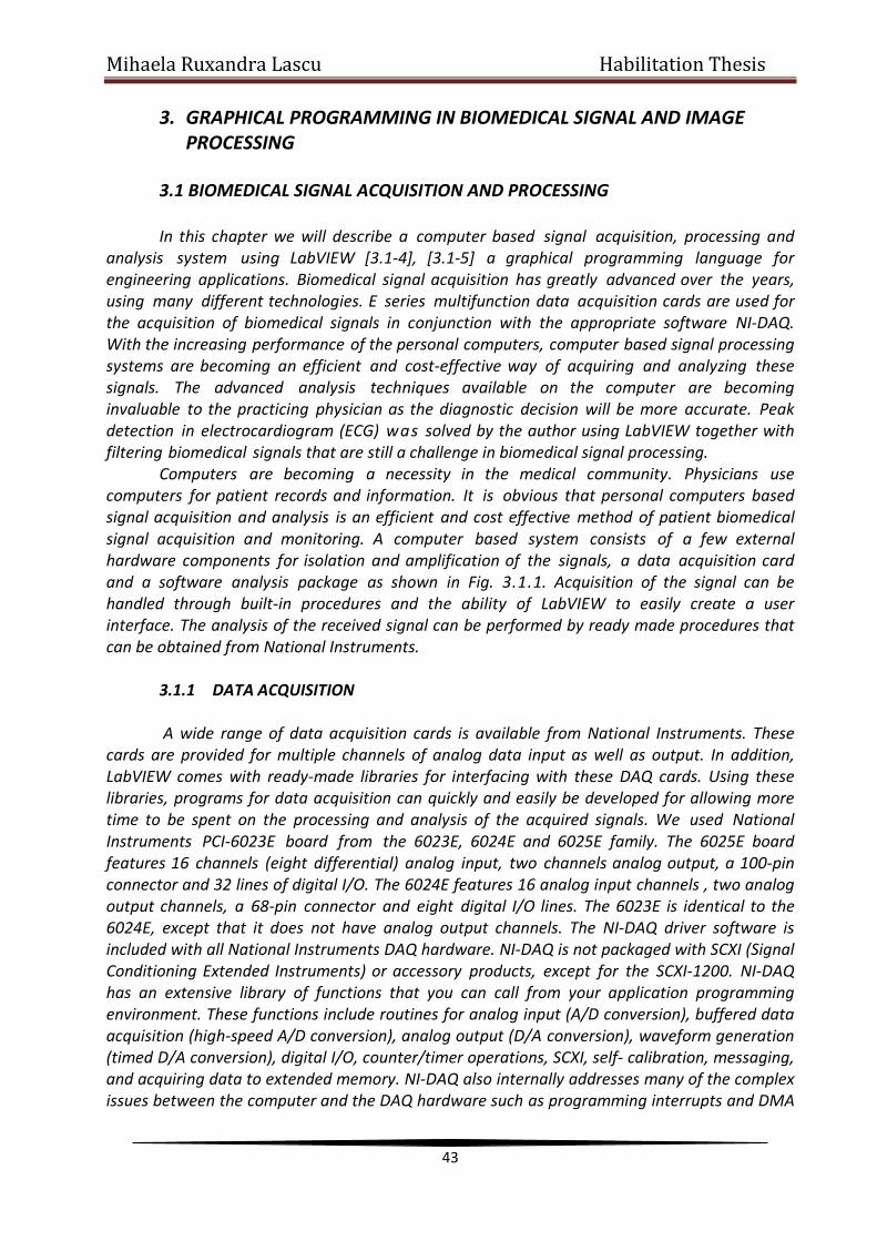
Mihaela Ruxandra Lascu Habilitation Thesis
43
3. GRAPHICAL PROGRAMMING IN BIOMEDICAL SIGNAL AND IMAGE PROCESSING
3.1 BIOMEDICAL SIGNAL ACQUISITION AND PROCESSING
In this chapter we will describe a computer based signal acquisition, processing and analysis system using LabVIEW [3.1-4], [3.1-5] a graphical programming language for engineering applications. Biomedical signal acquisition has greatly advanced over the years, using many different technologies. E series multifunction data acquisition cards are used for the acquisition of biomedical signals in conjunction with the appropriate software NI-DAQ. With the increasing performance of the personal computers, computer based signal processing systems are becoming an efficient and cost-effective way of acquiring and analyzing these signals. The advanced analysis techniques available on the computer are becoming invaluable to the practicing physician as the diagnostic decision will be more accurate. Peak detection in electrocardiogram (ECG) was solved by the author using LabVIEW together with filtering biomedical signals that are still a challenge in biomedical signal processing.
Computers are becoming a necessity in the medical community. Physicians use computers for patient records and information. It is obvious that personal computers based signal acquisition and analysis is an efficient and cost effective method of patient biomedical signal acquisition and monitoring. A computer based system consists of a few external hardware components for isolation and amplification of the signals, a data acquisition card and a software analysis package as shown in Fig. 3.1.1. Acquisition of the signal can be handled through built-in procedures and the ability of LabVIEW to easily create a user interface. The analysis of the received signal can be performed by ready made procedures that can be obtained from National Instruments.
3.1.1 DATA ACQUISITION
A wide range of data acquisition cards is available from National Instruments. These
cards are provided for multiple channels of analog data input as well as output. In addition, LabVIEW comes with ready-made libraries for interfacing with these DAQ cards. Using these libraries, programs for data acquisition can quickly and easily be developed for allowing more time to be spent on the processing and analysis of the acquired signals. We used National Instruments PCI-6023E board from the 6023E, 6024E and 6025E family. The 6025E board features 16 channels (eight differential) analog input, two channels analog output, a 100-pin connector and 32 lines of digital I/O. The 6024E features 16 analog input channels , two analog output channels, a 68-pin connector and eight digital I/O lines. The 6023E is identical to the 6024E, except that it does not have analog output channels. The NI-DAQ driver software is included with all National Instruments DAQ hardware. NI-DAQ is not packaged with SCXI (Signal Conditioning Extended Instruments) or accessory products, except for the SCXI-1200. NI-DAQ has an extensive library of functions that you can call from your application programming environment. These functions include routines for analog input (A/D conversion), buffered data acquisition (high-speed A/D conversion), analog output (D/A conversion), waveform generation (timed D/A conversion), digital I/O, counter/timer operations, SCXI, self- calibration, messaging, and acquiring data to extended memory. NI-DAQ also internally addresses many of the complex issues between the computer and the DAQ hardware such as programming interrupts and DMA

Mihaela Ruxandra Lascu Habilitation Thesis
44
controllers. NI-DAQ maintains a consistent software interface among its different versions so that you can change platforms with minimal modifications to your code. Either we are using conventional programming languages or National Instruments application software, our application uses the NI-DAQ driver software [3.1-4], [3.1-5] as illustrated in Fig.3.1.2.
Fig.3.1.1. Computer based biomedical signal acquisition and analysis system.
After installing NI-DAQ device drivers we obtain on the desktop of the computer an icon named Measurement and Automation Explorer (MAX). This program is necessary for identifying the presence of the DAQ-card and for setting the channels that will be used. MAX provides access to our PCI-6023E DAQ acquisition card. MAX can manage devices and interfaces, the installed National Instruments software, virtual channels or tasks for the used devices and also it can create scales for the created virtual instrument, can configure the Interchangeable Virtual Instrument (IVI) drivers and import/export the device configuration file.
The boards have three different input modes— nonreferenced single-ended (NRSE) input, referenced single-ended (RSE) input and differential (DIFF) input. The RSE configuration provides
up to 16 channels. The DIFF input configuration provides up to eight channels. Input modes are
programmed on a per channel basis for multimode scanning. It is possible to configure the
circuitry to scan 12 channels - four differentially configured channels and eight single-ended
channels. Table 3.1.1 describes the three input configurations. Because it was not possible to
make an acquisition of a biomedical signal in real time, at the beginning we have studied the possibility for an electrocardiograph realization, that means the acquisition of a sinusoidal signal
of 1 mV amplitude and 1-2Hz frequency from a function generator. Then we have performed
the acquisition of a biomedical signal that is specific for the heart activity.
An overview of the hardware functions of the PCI-6023E board is presented in Fig.3.1.3.
Fig.3.1.2. Relationship between the programming environment, NI-DAQ and DAQ-Card.

Mihaela Ruxandra Lascu Habilitation Thesis
45
Fig.3.1.3. Typical block diagram of 6023E, 6024E and 6025E acquisition cards.
Table 3.1.1
Configurations Description
DIFF A channel configured in DIFF mode uses two analog
input lines. One line connects to the positive input of
the programmable gain instrumentation amplifier (PGIA), and the other connects to the negative input of
the PGIA.
RSE A channel configured in RSE mode uses one analog
input line, which connects to the positive input of the
PGIA. The negative input of the PGIA is internally tied to analog input ground (AIGND).
NRSE A channel configured in NRSE mode uses one analog
input line, which connects to the positive input of the PGIA. The negative input of the PGIA connects to
analog input sense (AISENSE).
Using the block diagram in Fig.3.1.4, we build an acquisition and a visualisation of the
real signal and the processed signal. Because there are a lot of imperfect connexions from an electronic point of view, there are a lot of long linking wires in a polluted electromagnetic environment and the input impedance is high, the acquired signal is noise disturbed. For filtering the disturbed signal it is necessary to cascade two filters: the first filter is a low-pass one having with a 40Hz cut-off frequency while the second filter is an averaging Hanning filter [3.1-2].
When an ensemble of several realizations of an event is not available, synchronized averaging will not be possible. We are then forced to consider temporal averaging for noise

Mihaela Ruxandra Lascu Habilitation Thesis
46
removal, under the assumption the processes involved are ergodic. Therefore temporal statistics may be used instead of ensemble statistics. As temporal statistics are computed using a few samples of the signal along the time axis and the temporal window of samples is moved to obtain the output at various points of time, such a filtering procedure is called a moving- window averaging filter. The term moving- average (MA) filter is commonly used and is implemented in LabVIEW by the help of shift-registers.
The general form of an MA filter is:
,knxbnyN
0kk
(3.1.1)
where x and y are the input and output of the filter, respectively. The b values are the filter coefficients or tap weights, k = 0, 1, 2,..., N, where N is the order of the filter. The effect of division by the number of samples used (N+1) is included in the values of the filter coefficients. Applying the z-transform, we get the transfer function of the filter, H(z), as:
NN
110
N
0k
kk zb...zbbzb
zX
zYzH
(3.1.2)
where X(z) and Y(z) are the z-transforms of x(n) and y(n), respectively. A simple MA filter for filtering noise is the Hanning (Hann) filter [3.1-2], given by
.2nx1nx2nx4
1ny (3.1.3)
The Analog Input Multipoint Block that was used in the block diagram communicates with the data acquisition system and makes the acquisition of an external signal. We use an analog channel with the following characteristics. The name of the channel is Ecg1; the channel is programmed for signal input RSE (unipolar signal); the input range [−5mV ,+5mV ]; the
number of samples inside one acquisition is 100; the sampling frequency is 200Hz. The first three characteristics are appointed by MAX, that is capable to communicate to
any National Instruments data acquisition card. The last two properties are introduced with LabVIEW, that means the values and the name of the channel are selected from the controls belonging to the front panel; the terminal sources from the block diagram take these new values and channel name and updates the acquisition.
After running the above program we can indicate the three graphs that meet the necessity to display the input signal, the low-pass filtered signal and the averaging with the Hanning filter. The signals that have been acquisitioned and processed according to the presented theory are depicted in Fig.3.1.5. and Fig.3.1.6. Two acquisitions, for two different electrocardiograms are performed with the PCI-6023E card. The easiest way to acquire a single waveform from a single channel is to use the AI Acquire Waveform virtual instrument [3.1-1].

Mihaela Ruxandra Lascu Habilitation Thesis
47
Fig.3.1.4. Part of electrocardiogram acquisition and processing block diagram.
Using this virtual instrument it is necessary to specify a device and/or channel, the number of samples to acquire from the channel and the sample rate measured in samples per second. It is also possible to programmatically set the gain by setting the high limit and the low limit. Using only the minimal set of inputs makes programming the virtual instrument easier, but the virtual instrument lacks more advanced capabilities, such as triggering. It is also possible to acquire more than one waveform at a time with another Easy Analog Input VIs, AI Acquire Waveforms. This virtual instrument has also a minimal set of inputs, but it allows inputs of more than one channel to be read and return an array of waveforms from all channels it reads. To access or control an individual waveform, I have indexed the array of waveforms with the Index Array function or one can use input indexing on a For or While Loop. A two channel data acquisition system can be build as in Fig.3.1.7.
Fig.3.1.5. Electrocardiogram and low pass filtered electrocardiogram.

Mihaela Ruxandra Lascu Habilitation Thesis
48
Fig.3.1.6. Electrocardiogram with 60Hz noise (upper graph), filtered electrocardiogram (middle graph)
and averaged electrocardiogram Hanning filter (low graph).
In this program we have the possibility to choose the channel, the frequency, the device and the sampling rate. To acquire multiple waveforms it is also possible using the Intermediate virtual instruments.
The biomedical signals acquired from the human body are frequently very small, often in the millivolt range, and each has its own processing needs. Electroencephalography signals are in the microvolt range and have many frequency components. Obviously, these biomedical signals require to be processed before they will be analyzed. LabVIEW contains the tools, from fast Fourier transforms to digital filters, to realize complex analysis. In order to perform frequency analysis, a complex signal must first be broken down into its frequency components. One of the most common way to do this is with the FFT. In order to facilitate this type of analysis, LabVIEW comes with built in FFTs that make the process of component separation quick and easy. In addition, biomedical signals being very small are in danger to be overwhelmed by noise. To prevent this it is necessary to use a SCXI card that means to run the acquired signal through a set of filters and amplifiers [3.1-5]. However, after the signal reaches the computer, it can still contain noise. Another way to solve the noise problem is to use the digital filters provided with LabVIEW. LabVIEW offers the choice of Butterworth, Bessel, Chebyshev and digital filters. With a few adjustments these filters can be configured for almost any design that is needed. A dual channel spectral measurement with filter is presented using the Express virtual instruments that have the possibilities to choose different kind of parameters from their internal implementation. The block diagram is represented in Fig.3.1.8. The steps implemented are described below. The first step is to simulate the biomedical signal using a DC signal generation with uniform white noise. The second step is filtering the signal with a bandpass filter. The third step consists of two parts: updating the Waveform Graph cursors to represent the current values of the upper and lower cut-off frequencies and checking to see if the upper or lower cut-off frequency values have changed since the last iteration. If so it is necessary to reset the Dual Spectral Measurement averaging. The fourth step performs a Dual Channel Spectral Measurement both on the prefiltered signal and the filtered signal in order to determine the frequency response of the filter. In the last step the calculated filter frequency response against preset specifications is determined and it is checked whether the filter meets the requirements or not. For the simulation we have used the uniform white noise because it covers the entire frequency range.

Mihaela Ruxandra Lascu Habilitation Thesis
49
Fig.3.1.7. Two channel data acquisition system.
In this way the Dual Channel Spectral Measurement Express virtual instrument easily determines what frequencies are being filtered out. For the signal display, several signals can be displayed on the same chart or separate charts can be configured for each signal. LabVIEW offers sweep, scope and strip charts; a sweep chart sends a vertical line along with the signal from left to right so that the new data is to the left of the line, while the old is on the right. With a scope chart the signal travels from left to right and when it reaches the right edge, the chart screen is refreshed. The most common chart type for biomedical signals, however, is the strip chart; strip charts bring the new data in, on the right side of the screen, while the old travels off to the left. One of the greatest benefits of this chart type is the ability to view past data using a scrollbar attached to the chart. Analysis of the biomedical signals can also be easily performed in LabVIEW. The graphical nature of LabVIEW allows even the beginner programmer to easily write programs to analyze data without having to worry about the syntax problems associated with most programming languages. In Fig.3.1.9 is represented a peak detection in an electrocardiogram – Front Panel and Block Diagram. Using LabVIEW and the virtual instrument named Peak Detector we can obtain the desired diagnostic decision. These prebuilt modules are extremely useful in complicated applications.

Mihaela Ruxandra Lascu Habilitation Thesis
50
Fig.3.1.8. A dual channel spectral biomedical signal measurement with filter using Express VIs.
We have established the peaks for different biomedical signal types. Peak detection is
the first step in event detection [3.1-2], [3.1-4], [3.1-5]. Finally, we can say that event detection is an important step that is acquired before attempting to analyze the corresponding waves or wavelets [3.1-3]. After a specific wave of interest has been detected, isolated and extracted, methods targeted to the expected characteristics of the event may be applied for analysis of the corresponding physiological or pathological event. We can use this Peak Detection in an application like an ECG Rhythm analysis. The output of the final smoothing filter that passed the ECG signal could be subjected to a peak- searching algorithm to obtain a time marker for each QRS or ECG beat. The intervals between two such consecutive markers give the RR interval, which could be averaged over a number of beats to obtain a good estimate of the inter-beat interval. The heart rate may be computed in bpm as 60 divided by the average RR interval in seconds. The heart rate may also be obtained by counting the number of beats detected over a certain period.
Fig.3.1.9. Peak detection in an electrocardiogram.

Mihaela Ruxandra Lascu Habilitation Thesis
51
3.1.2 LABVIEW FOR ECG MATERNAL AND FETAL SIGNAL
Biomedical signal processing algorithms form an important part of real-time systems for monitoring the patients who suffer from a life-threatening condition. Such systems are usually designed to detect changes in cardiac or neurological function and to predict the outcome of a patient admitted to the intensive care unit [3.1-1], [3.1-2]. Since such changes may be reversible with early intervention, irreversible damage can sometimes be prevented. Similar to therapeutic context, the signal is processed during monitoring in an essentially sequential fashion, such that past samples constitute the main basis for a decision, while just a few seconds of the future samples may also be considered - a property which usually stands in sharp contrast to signal processing for diagnostic purposes, where the signal is acquired in its entirety prior to analysis.
The fetal electrocardiogram can be derived from the maternal abdominal ECG and can be used for the extraction of fetal heart rate, which indicates the cardiac condition of the fetus. The locations of leads for an 8-channel maternal ECG acquisition system are shown in Fig. 3.1.10. Maternal thorax ECG signals are sampled from thorax leads while maternal abdominal ECG signals are obtained from abdominal leads. In Fig. 3.1.11 are depicted the Advanced Signal Processing Toolkit (ASPT) and the Digital Filter Design Toolkit (DFDT). The Express VI Development Toolkit is conveniently to use for building signal processing applications as baseline wandering removing, noise cancellation, QRS complexes detection and fetal heart rate extraction.
Fig.3.1.10. Thorax leads and abdominal leads for maternal and abdominal ECG acquisition.
Fig.3.1.11. Digital filter design and advanced signal processing toolkits.
In Fig.3.1.12 an ECG signal recorded from the abdomen of a pregnant woman is shown.
An ECG from the woman’s chest is recorded. Monitoring the two ECG signals, we observe that the abdominal ECG exhibits multiple peaks because the QRS complexes are corresponding to the maternal ECG that occur at the same time instants with the QRS thorax complexes. The non-maternal QRS complexes represent the ECG of the fetus.

Mihaela Ruxandra Lascu Habilitation Thesis
52
It is necessary to observe that the QRS complex shapes of the maternal ECG from the chest and abdominal leads have different shapes due to the projection of the cardiac electrical vector onto different axes. Considering that the two signals being combined have almost the same bandwidth it is necessary to separate them and obtain the fetal ECG. Generally, the recorded ECG signal is often contaminated by noise and artifacts that can be within the frequency band of interest and manifest with similar characteristics as the ECG signal itself. In order to extract useful information from the noisy ECG signals, it is necessary to process the raw ECG signals.
Fig.3.1.12. ECG signals of a pregnant woman from abdominal and chest leads: a) chest leads ECG, and b)
abdominal lead ECG.
ECG signal processing can be roughly divided into two stages by functionality: preprocessing and feature extraction (as shown in Fig.3.1.13). The preprocessing stage removes or suppresses noise from the raw ECG signal and the feature extraction stage extracts diagnostic information from the ECG signal [3.1-1], [3.1-2], [3.1-3], [3.1-5], [3.1-6].
Fig.3.1.13. Preprocessing ECGs records and feature extraction.
Preprocessing ECG signals is necessary to remove contaminants from the ECG signals.
Roughly speaking, ECG contaminants can be classified into the following categories: power line interference, electrode pop or contact noise, patient–electrode motion artifacts, electromyography (EMG) noise, and baseline wandering. The LabVIEW provides an intuitive and interactive way to design and implement finite impulse response (FIR) or infinite impulse response (IIR) filters easily and effectively.
We used the Configure Classical Filter Design Express VI to design a Kaiser Window FIR highpass filter to remove the baseline wandering. The configuration is built for a sampling frequency of 200Hz and 1000Hz. Figure 3.1.14.a and 3.1.14.b show an example of the specifications for the highpass filter and the block diagram of a simple virtual instrument that you can use to remove the baseline wandering.

Mihaela Ruxandra Lascu Habilitation Thesis
53
a)
b)
Fig.3.1.14 a) Highpass filter front panel used to remove baseline wandering with sampling frequency 200Hz.
b) Highpass filter front panel used to remove baseline wandering with sampling frequency 1000Hz. Concerning the stability of the system, the position of the poles is inside the unit circle
and the zeroes are inside and outside. It is possible to observe in Fig.3.1.14.a that zeros are equidistant to the unit circle for 200Hz sampling frequency and in Fig.3.1.14.b for 1000Hz sampling frequency. It is also possible to change the window. For example, window Dolph-Chebyshev assures equidistance between zeros and poles inside the circle as well. Stability is also assured in this situation.
Independent Component Analysis (ICA) is a method for retrieving independent hidden signals from a multi-channel observation. Assuming that the observation X is a superposition of the source signals S, it is possible to write that 𝑿 = 𝑨 ∙ 𝑺, where A denotes a mixing matrix.

Mihaela Ruxandra Lascu Habilitation Thesis
54
The assumption of statistical independence of the signals S allows you to estimate both unknowns, S and A, from the observation X. Here, the maternal ECG and the fetal ECG can be treated as independent components i.e. they are parts of S, while the 8-channel measured ECG records constitute X. By performing ICA, you can obtain the estimation of S, which means you can get both maternal ECG and fetal ECG.
The ASPT provides the Time Sample Analysis (TSA) Independent Component Analysis VI with which you can easily build a Fetal Heart Rate (FHR) extraction application, as shown in Fig.3.1.15. The inputs of the ICA function are 8-channel ECG signals (acquired by the 8- channel system mentioned before) and the fetal ECG signal can be obtained from the output as one of the independent components. Fig. 3.1.15 shows the implemented ICA method as a block diagram for extracting the maternal abdominal ECG and the fetal ECG.
Fig.3.1.15. ICA method for fetal heart rate extraction.
ECG Baseline Remove. One common variety of exercise induced artifacts is baseline
wander resulting from movement, respiration, and poor electrode contact. Although filters can be designed to remove much of this baseline variation, they will distort the low-frequency components of the ECG complex, such as the TP-segment, the PR-segment and most problematically, the ST-segment. The ST-segment is the most diagnostically relevant measure of the ECG taken during exercise. While linear baseline interpolation and removal may be adequate at lower heart rates, they also will introduce significant distortions. This is particularly evident when excessive nonlinear wander is present, as seen at higher heart rates and respiration rates. Since the cubic spline is not a filter and uses an a priori knowledge of the ECG signal shape, it estimates the true baseline and better avoids distortion. The most common implementations of this technique use relatively short ECG recordings. With the advent of increasing power in computerized ECG systems, the implementation of the cubic spline algorithm for removing baseline wander in continuous, longer-duration ECG records and in real-time processing is being attempted. However, the correct application of the cubic spline to continuous recordings is not straightforward and involves a number of previously unforeseen difficulties. The accuracy and resolution of both floating point and integer operations is critical during long-term application of the cubic spline function.
After removing the baseline wandering as in Fig.3.1.16, the resulting ECG signal is more stationary and explicit than the original signal. However, some other types of noise might still affect feature extraction of the ECG signal. The noise may be a complex stochastic process

Mihaela Ruxandra Lascu Habilitation Thesis
55
within a wideband, so you cannot remove them by using traditional digital filters. To remove the wideband noises, you can use the Wavelet Denoise Express VI as in Figure 3.1.17 a, b:
Fig.3.1.16. Block diagram designing and using a highpass filter to remove baseline wandering.
a)
b)
Fig.3.1.17. a) ECG Wavelet Denoise Express Virtual Instrument.
b) ECG Wavelet Denoise Express Virtual Instrument and characteristic window for Wavelet Denoise.
This ECG Wavelet Express VI first decomposes the ECG signal into several subbands
by applying the wavelet transform [3.1-3], [3.1-6] and then modifies each wavelet coefficient by applying a threshold or shrinkage function and finally reconstructs the denoised signal.
The data source can be from a terminal or from a file. “From terminal” specifies that the virtual instrument reads data from the block diagram input. “From file” specifies that the virtual instrument reads data from a file. The virtual instrument can read data from waveform, WAV, or text, TXT, files. The virtual instrument processes the data from WAV files as a waveform data type. The valid format of a TXT data file is a file that contains only a 1D real array, a 2×m real

Mihaela Ruxandra Lascu Habilitation Thesis
56
matrix or an m×2 real matrix. The virtual instrument processes the 1D real array from TXT data files as a real data type. The 2×m real matrix or the m×2 real matrix from a TXT data file are processed as complex data type. The virtual instrument treats the first row or column as the real part of the data and the second row or column as the imaginary part of the data.
File Path Configuration contains the following options. File path — Specifies and displays the full path to the file from which we want to read data. Ask user to choose a file each time this VI runs — Displays a dialog box that prompts users to select a file each time the virtual instrument runs. This Express Virtual Instrument displays the original signal and the signal after denoising. The transform settings contain the following options.
Transform type — Specifies the use of the discrete wavelet transform or undecimated wavelet transform to denoise the signal. Wavelet — specifies the wavelet type to use for the discrete wavelet analysis. The default is db02. The options include two types: orthogonal (Haar, Daubechies (dbxx), Coiflets (coifx), Symmlets (symx)) and biorthogonal (FBI, Biorthogonal (biorx_x)), where x indicates the order of the wavelet. The higher the order, the smoother the wavelet. The orthogonal wavelets are not redundant and are suitable for signal or image denoising and compression. The biorthogonal wavelets usually have the linear phase property and are suitable for signal or image feature extraction.
Threshold settings contain the following options. Soft threshold —specifies to use the soft thresholding method. The default is to use the soft thresholding method. If you remove the checkmark from the Soft threshold checkbox, the virtual instrument uses the hard thresholding method. Thresholding rule —specifies the threshold selection rules. The default is SURE, which indicates that the virtual instrument uses the principle of Stein's Unbiased Risk Estimate (SURE) to estimate the threshold. If you select Hybrid, the virtual instrument finds a compromise between the SURE method and the Universal Method. When the signal-to-noise ratio of the noisy signal is very low, the virtual instrument uses the Universal Method to estimate the threshold. If you select Universal, the virtual instrument sets the threshold to sqrt (2×log (Ls)), where Ls is the signal length. If you select Minimax, the virtual instrument uses the Minimax Principle to estimate the threshold. Rescaling method — specifies the method used to estimate the noise variance at each level. The default is single level, which indicates that the noise is white and that the virtual instrument estimates the noise standard deviation from the wavelet coefficients at the first level. The virtual instrument uses the noise variance to rescale the threshold. Therefore, you can update the thresholds with the noise variance. Selecting one indicates that the noise is white with unit variance. Selecting multiple levels indicates that the noise does not have to be white and that the virtual instrument estimates the noise standard deviation at each level independently. Option for approximation — specifies the operation for the approximation coefficients from the wavelet decomposition. The default is none, which indicates that the virtual instrument keeps the approximation coefficients unchanged. If you select threshold, the virtual instrument applies the same thresholding operation to the approximation coefficients. If you select detrend, the virtual instrument sets the approximation coefficients to 0. In the last few years [3.1-3], [3.1-5] wavelets have emerged as a powerful tool for extracting signals from noisy data. For the case of Gaussian white noise, the signal extraction problem can be stated as follows: we determine the true values of a signal Sz given by:

Mihaela Ruxandra Lascu Habilitation Thesis
57
nit
;tSS
;tSS
,1n,...,0i,zSS
i
ii
izz
i
iizi
(3.1.4)
where is the standard deviation of the noise and zi are random variables according to N(0,1).
In the wavelet domain we can rewrite:
.zWSWSSWSW iiiizi (3.1.5)
3.2 GRAPHICAL PROGRAMMING IN EVENT DETECTION USING PAN TOMPKINS ALGORITHM
QRS and ventricular beat detection is a basic procedure for electrocardiogram (ECG)
processing and analysis. Large variety of methods have been proposed and used, featuring high percentages of correct detection. Nevertheless, the problem remains open, especially with respect to higher detection accuracy in noisy ECGs. We developed in LabVIEW the filtering for removal of artifacts in biomedical signals and the Pan-Tompkins algorithm. We have investigated problems posed by artifact, noise and interference of various forms in the acquisition and analysis of several biomedical signals. We have also established links between the characteristics of certain events in a number of biomedical signals and the corresponding physiological or pathological events in the biomedical systems of concern. Event detection is an important step that is required before we may attempt to analyze the corresponding waves in more detail.
Biomedical signals are fundamental observations for analyzing the body function and for diagnosing a wide spectrum of diseases. The problems caused by artifacts in biomedical signals are vast in scope and variety; their potential for degrading the performance of the most sophisticated signal processing algorithms is high.
An ECG signal [3.2-1] can be disturbed by a high frequency noise. The noise is due to the instrumentation amplifiers, the recording system and pickup of ambient electromagnetic signals by the cables. The signal can also be corrupted by power-line interference at 50Hz or 60Hz and its harmonics, which may also be considered as a part of high-frequency noise relative to the low- frequency nature of the ECG signal.
Low-frequency artifacts and base-line drift may be caused in chest-lead ECG signals by coughing or breathing with large movement of the chest. Poor contact and polarization of the electrodes may also cause low-frequency artifacts. Base line drift may sometimes be caused by variations in temperature and bias in the instrumentation and amplifiers as well. The most commonly encountered periodic artifact in biomedical signals is the power-line interference at 50Hz or 60Hz. If the power-line waveform is not a pure sinusoid due to distortions or clipping, harmonics of the fundamental frequency could also appear. Harmonics will also appear if the interference is a periodic waveform that is not a sinusoid. Power-line interference may be difficult to visually be detected in signals being non-specific waveforms; however, the interference is easily visible if present on well-defined signal waveforms such as the ECG or carotid pulse signals. In either case, the power spectrum of the signal should provide a clear indication of the power line interference presence as an impulse or spike at

Mihaela Ruxandra Lascu Habilitation Thesis
58
50Hz or 60 Hz; harmonics will appear as additional spikes at integral multiples of the fundamental frequency.
The QRS complexes and ventricular beats in an electrocardiogram represent the depolarization phenomenon of the ventricles and yield useful information about their behavior. Beat detection is a procedure preceding any kind of ECG processing and analysis. For morphological analysis this is the reference for detection of other ECG waves and parameter measurements. Rhythm analysis requires classification of QRS and other ventricular beat complexes as normal and abnormal. Real-time ventricular beat detection is essential for monitoring of patients in critical heart condition.
3.2.1 FILTERING FOR ARTIFACTS REMOVAL
Information provided by bioelectric signals are generally time-varying, nonstationary,
sometimes transient, and usually corrupted by noise. Fourier transform has been the unique tool to face such situations, even if the discrepancy between theoretical considerations and signal properties has been emphasized for a long time. These issues can be now nicely addressed by time-scale and time frequency analysis.
One of the major areas where new insights can be expected is the cardiovascular domain. For diagnosis purpose, the noninvasive electrocardiogram ECG is of great value in clinical practice. The ECG is composed of a set of waveforms resulting from atrial and ventricular depolarization and repolarization. The first step towards ECG analysis is the inspection of P, QRS and T waves see Fig.3.2.1; each one of these elementary components is a series of onset, offset, peak, valley and inflection points. Ideally, the waves exhibit local symmetry properties with respect to a particular point, peak and inflection points locations of the considered wave. Based on these properties, one can extract significant points to study the wave shapes and heart rate variability.
In my work I have gained an understanding of a few sources of artifacts in biomedical signals and their nature and I can now tackle specific problems and develop effective filtering techniques to solve them.
The proposed solution provides the details of an appropriate filtering technique. Certain types of noise may be directly filtered in the time domain using signal processing techniques or digital filters. An advantage of time-domain filtering is that spectral characterization of the signal and noise may not be required. Linear filters fail to perform when the signal and noise spectra overlap. Synchronized signal averaging can separate a repetitive signal from noise without distorting the signal [3.2-1]. A synchronized averaging is a type of ensemble averaging. An algorithmic description of synchronized averaging is as follows: a) obtain a number of realizations of the signal or event of interest; b) determine a reference point for each realization of the signal; c) extract parts of the signal corresponding to the events and add them to the buffer, being possible that the different parts are of different durations; d) divide the result in the buffer by the number of events added.
Let yk (n) be one realization of a signal with k=1,2,…,L representing the ensemble index and n=1,2,…, N representing the time-sample index. The observed signal is
,nnxny kkk (3.2.1)
where xk(n) is the original uncorrupted signal and k(n) is the noise in the kth copy of the observed signal.

Mihaela Ruxandra Lascu Habilitation Thesis
59
Fig.3.2.1. Example of a normal ECG beat.
If for each instant of time n we add L copies of the signal, we get:
.N,...,2,1n;nnxnyL
1kk
L
1kk
L
1kk
(3.2.2)
If the repetitions of the signal are identical and aligned, then
.nLxnxL
1kk
(3.2.3)
If the noise is random with zero mean value and variance 2, then ∑ 𝜂𝑘(𝑛)𝑙
𝑘=1 𝑤𝑖𝑙𝑙 tend to zero as L increases with a variance of 𝑀𝜎𝜂
2. The RMS value of the noise in the averaged signal is
√𝑀𝜎𝜂. Thus the SNR of the signal will increase by a factor √𝐿.
The larger the number of events that are averaged, the higher will be the SNR of the result. Fig.3.2.2 illustrates two ECG cycles extracted using the trigger points obtained by thresholding the crosscorrelation function [3.2-1], as well as the result of averaging the first 11cycles in the signal.
Fig.3.2.2. The upper two traces - two cycles of the ECG extracted from an ECG signal with noise. The
bottom trace – the result of synchronized averaging over 11 cycles from the same ECG signal.
Structured noise such as power-line interference may be suppressed by synchronized averaging if the phase of the interference in each realization is different. When an ensemble of several realisations of an event is not available, synchronized averaging will not be possible. In this case we consider temporal averaging for noise removal, under the assumption that the processes involved are ergodic and consequently temporal statistics may be used instead of ensemble statistics.
The biomedical signals that have been processed are from the following online biomedical signals databases: ftp://ftp.ieee.org/uploads/press/rangayyan,www.ecgdatabase.com, www.ecglibrary.com.

Mihaela Ruxandra Lascu Habilitation Thesis
60
HIGH FREQUENCY NOISE IN THE ECG The Butterworth filter is perhaps the most commonly used frequency domain filter due
to its simplicity and the property of a maximally flat magnitude response in the pass-band [3.2-2]. The basic Butterworth lowpass filter function is:
aN2
C
2a H
j
j1
1jH
(3.2.4)
where 𝐻𝑎 is the frequency response of the analog filter and 𝛺𝑐 is the cutoff frequency in radians/s and N is the order of the filter. As the order N increases, the filter response becomes more flat in the pass-band and the transition to the stop-band becomes sharper.
Changing to the Laplace variable s, we get:
;
j
s1
1sHsH
N2
C
aa
(3.2.5)
Using the bilinear transformation 𝑠 =2
𝑇
1−𝑧−1
1+𝑧−1, we obtain the following simplified
transfer function in the z domain:
;
za
z1GzH
N
0k
kk
N1|
(3.2.6)
where 𝑎𝑘, k=0,1,2,…,N, are the filter coefficients and G’ is the gain factor at z=1. The filter is now in the familiar form of an IIR filter. Realization of a generic IIR filter is illustrated as signal-flow diagram in Fig. 3.2.3.
A LabVIEW program for eliminating the high frequency noise based on the IIR filter was developed and the graphs concerning the input signal and the output signal processed with the IIR filter are presented in Fig.3.2.4. LOW FREQUENCY NOISE IN THE ECG
Low-frequency artifacts and base-line drift in chest-lead ECG signals may be caused by coughing or breathing with large movement of the chest. Poor contact and polarization of the electrodes may also cause low-frequency artifacts. Base line drift may sometimes be caused by variations in temperature and bias in the instrumentation and amplifiers as well.
The drawback of the first-order difference and the three-point central-difference operators [3.2-1] lies in the fact that their magnitude response remains low for a significant range of frequencies well beyond the band related to the base-line wander. We would like to maintain the levels of the components present in the signal beyond about 0.5-1Hz, that is, we would like the gain of the filter to be close to unity after about 0.5Hz.

Mihaela Ruxandra Lascu Habilitation Thesis
61
Fig.3.2.3. Signal-flow diagram in a direct realization of a generic infinite impulse response filter.
The gain of a filter at specific frequencies may be boosted by placing poles at related locations around the unit circle in the z-plane. For the sake of filter stability, the poles should be placed within the unit circle. Since we are interested in maintaining a high gain at very low frequencies, we could place a pole on the real axis (zero frequency), say at z=0,995 [3.2-2]. The transfer function of the modified first-order difference filter is then:
1
1
z995.01
z1
T
1zH (3.2.7)
or
995.0z
1z
T
1zH (3.2.8)
The time-domain input-output relationship is given as:
1ny995.01nxnxT
1ny (3.2.9)
The LabVIEW program and the obtained waveforms are represented in Fig.3.2.5:

Mihaela Ruxandra Lascu Habilitation Thesis
62
Fig.3.2.4. LabVIEW program based on IIR filter: high frequency noise signal (upper graph) and filtered
signal (lower graph).

Mihaela Ruxandra Lascu Habilitation Thesis
63
Fig.3.2.5. The LabVIEW block diagram program based on the derivative operator. Low frequency noise signal in the upper graph and filtered signal in the lower graph.
POWER-LINE INTERFERENCE IN ECG SIGNALS The simplest method to remove periodic artifacts is to compute the Fourier transform of
the signal, delete the undesired components from the spectrum and then compute the inverse Fourier transform. The undesired components could be set to zero, or better, to the average level of the signal components over a few frequency samples around the component that is to be removed. Periodic interference may also be removed by notch filters [3.2-1] with zeros on the unit circle in the z-domain at the specific frequencies to be rejected. Applying the LabVIEW program we obtain the results presented in Fig.3.2.6.

Mihaela Ruxandra Lascu Habilitation Thesis
64
Fig.3.2.6. Random noise elimination using notch filter and Hanning filter.
3.2.2 THE PAN-TOMPKINS ALGORITHM FOR QRS DETECTION
Pan and Tompkins [3.2-3], [3.2-4], [3.2-5] proposed a real-time QRS detection algorithm
based on the analysis of the slope, amplitude and width of QRS complexes. The algorithm includes a series of filters and methods that perform lowpass, highpass, derivative, squaring, integration, adaptive thresholding and search procedures, as specified in Fig.3.2.7. In this work we implemented the Pan-Tompkins algorithm for QRS detection [3.2-1] in LabVIEW.
Fig.3.2.7. Block diagram of the Pan-Tompkins Algorithm for QRS detection.

Mihaela Ruxandra Lascu Habilitation Thesis
65
LOWPASS FILTER The recursive lowpass filter used in the Pan-Tompkins algorithm has integer coefficients for reducing computational complexity, with the transfer function defined as:
21
26
z1
z1
32
1zH (3.2.10)
From (3.2.10) the output y(n) is related to the input x(n) as:
.12nx6nx2nx32
12ny1ny2ny (3.2.11)
With the sampling rate being 200 Hz, the filter has a rather low cutoff frequency of fc=11Hz and
introduces a delay of 5 samples or 24ms. The filter provides an attenuation higher than 35dB at 60Hz and effectively supresses power-line interference, if present. HIGHPASS FILTER The highpass filter used in the algorithm is implemented as an allpass filter minus a lowpass filter. The lowpass component has the transfer function
1
32
lpz1
z1zH
(3.2.12)
and the input-output relationship:
.32nxnx1nyny (3.2.13)
The transfer function 𝐻ℎ𝑝(𝑧) of the highpass filter is specified as:
.zH32
1zzH lp
16lp
(3.2.14)
The output p(n) of the highpass filter is given by the difference equation:
.32nxnx1ny32
116nxnp (3.2.15)
where x(n) and y(n) being related as in (3.2.13). The highpass filter has a cutoff frequency of 5Hz and introduces a delay of 80 ms. DERIVATIVE OPERATOR The derivative operation used by Pan and Tompkins is specified as:
,4nx23nx1nxnx28
1ny (3.2.16)
and approximates the ideal 𝑑
𝑑𝑡 operator up to 30Hz. The derivative procedure suppresses the
low-frequency components of the P and T waves and provides a large gain to the high-frequency components arising from the high slopes of the QRS complex.

Mihaela Ruxandra Lascu Habilitation Thesis
66
SQUARING The squaring operation makes the result positive and emphasizes large differences resulting from QRS complexes; the small differences arising from P and T waves are suppressed. The high frequency components in the signal related to the QRS complex are further enhanced. INTEGRATION
As observed in the previous subsection, the output of the derivative-based operation will exhibit multiple peaks within the duration of a single QRS complex. The Pan Tompkins algorithm smoothes of the output of the preceding operations through a moving-window integration filter defined by:
.nx...2Nnx1NnxN
1ny (3.2.17)
The choice of the window width N is made taking into account the following considerations: a too large value will lead to merged outputs from the QRS and T waves, whereas a too small a value could yield several peaks for a single QRS. A window width of N=30 was found to be suitable for fs=200Hz. ADAPTIVE TRESHOLDING
The thresholding procedure in the Pan-Tompkins algorithm adapts to changes in the ECG signal by computing running estimates of signal and noise peaks. A peak is said to be detected whenever the final output changes direction within a specified interval. The running estimate of ECG signal peak (SPKI) represents the peak level that the algorithm has learned to be that corresponding to QRS peaks while the running estimate of the noise peak (NPKI) represents the peak level related to non-QRS events. THRESHOLDI1 and THRESHOLDI2 are two thresholds used to categorize peaks detected as signal or noise. Each new peak detected is categorized as a signal peak or as a noise peak. If a peak exceeds THRESHOLDI1 during the first step of analysis, it is classified to be a QRS peak. Using the searchback technique the peak should be above THRESHOLDI2 to be called a QRS. The peak levels and thresholds are updated after each peak is detected and classified as:
SPKI = 0.125PEAKI + 0.875SPKI if PEAKI is a signal peak; NPKI = 0.125PEAKI + 0.875NPKI if PEAKI is a noise peak; THRESHOLDI1=NPKI + 0.25(SPKI - NPKI); THRESHOLDI2=0.5THRESHOLDI1
The updating formula for SPKI is changed to SPKI = 0.25PEAKI + 0.75SPKI
if a QRS is detected in the searchback procedure [3.2-1], [3.2-3], [3.2-4] using THRESHOLDI2. Fig.3.2.7 illustrates the effect of the window width on the output of the integrator and its relationship to the QRS width.
Fig.3.2.7. Upper plot-Schematic ECG signal; Lower plot - Output of the moving-window integrator.
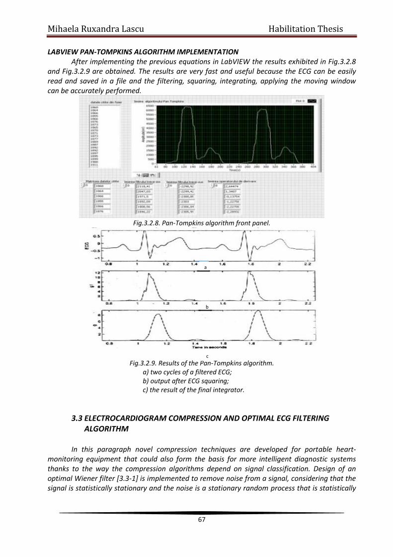
Mihaela Ruxandra Lascu Habilitation Thesis
67
LABVIEW PAN-TOMPKINS ALGORITHM IMPLEMENTATION After implementing the previous equations in LabVIEW the results exhibited in Fig.3.2.8
and Fig.3.2.9 are obtained. The results are very fast and useful because the ECG can be easily read and saved in a file and the filtering, squaring, integrating, applying the moving window can be accurately performed.
Fig.3.2.8. Pan-Tompkins algorithm front panel.
Fig.3.2.9. Results of the Pan-Tompkins algorithm. a) two cycles of a filtered ECG; b) output after ECG squaring; c) the result of the final integrator.
3.3 ELECTROCARDIOGRAM COMPRESSION AND OPTIMAL ECG FILTERING ALGORITHM
In this paragraph novel compression techniques are developed for portable heart-monitoring equipment that could also form the basis for more intelligent diagnostic systems thanks to the way the compression algorithms depend on signal classification. Design of an optimal Wiener filter [3.3-1] is implemented to remove noise from a signal, considering that the signal is statistically stationary and the noise is a stationary random process that is statistically
a
b
c

Mihaela Ruxandra Lascu Habilitation Thesis
68
signal independent. Two programs for compression and Wiener optimal filtering are developed in MATLAB.
The electrocardiogram (ECG) is one of the most important and widely used quantitative diagnostic tools in medicine. It is extremely useful for the diagnosis and management of heart abnormalities such as heart attacks and offers helpful clues to the presence of generalized disorders that affect the rest of the body, such as electrolyte disturbances and drug intoxication. ECGs can show long-term effects: previous cardiac events such as heart attacks that can result in permanent modification to the morphology of the ECG. Commercial ambulatory recorders typically have sample rates up to 360 samples per second with a resolution of 10 or 12 bit giving a bit rate of around 4000bit/s. A typical commercial sample rate of 256 samples per second with 10bit resolution on two channels over seven days implies a memory requirement of close to 400MB of data [3.3-3].
On top of the storage issue, there is an increasing interest in remote monitoring, using real-time or offline transmission of complete records. As a result, compression is a key concern for ECG equipment manufactures. Lossless compression refers to any scheme whereby the signal reconstructed after compression is identical in every respect to the original signal. By contrast, lossy schemes allow differences between the original and the reconstructed signal. The ECG is a real-world signal and is generally acquired from a relatively noisy electrical environment. Any lossless compression scheme has to reconstruct this random signal perfectly. This severely limits the effective compression ratio of lossless schemes when applied to ECG data. Lossless compression schemes may offer compression ratios of two or less. However, if restrictions on perfect reconstruction of the noise are relaxed, there is considerable room for enhancing performance by utilising knowledge concerning the morphology of the ECG and its cyclo-stationary characteristics.
Having established that lossy compression schemes offer the greatest ability for achieving useful compression ratios, two further categories may be identified within that class: direct and indirect transformation processes. Direct compression schemes are generally less computationally intensive and operate on the time-domain ECG signal, using relatively simple approaches such as piece-wise linear approximation. The highest compression ratio with the best reconstruction quality can only be achieved using indirect compression methods, also called transform methods.
The recognising beats techniques generally exploit the cyclo-stationary nature of the ECG record. The nature of the beats within the ECG must be understood. More specifically, deviations from the typical beat must be explicitly or implicitly recognised in order to efficiently represent them. A typical recording consists of a series of ECG beats separated by periods of inactivity, as illustrated in Fig.3.3.1.
Fig.3.3.1. A typical ECG recording of a normal subject, clearly showing the cyclo-stationary nature of the
ECG beat.

Mihaela Ruxandra Lascu Habilitation Thesis
69
Note that even when the heart rate varies, the basic morphology and temporal extent of the beat are relatively unchanged. The main difference appears with the gap between beats. Important sections of the beat are labeled as the P-wave, QRS complex, and the T-wave, as shown in the idealized waveform of Fig.3.3.2.
Fig.3.3.2. Idealised ECG beat, showing the P-wave, QRS-complex and T-wave.
In practice, there will often be two or more groups of beats, with each group having its own
distinct morphology. These differences may be clinically diagnosed. Similarities within a group are exploited using indirect compression schemes. Fig.3.3.3 shows the generic strategy used in many indirect compression methods, though a variant exists where the local DC removal step is omitted or carried out before triggering [3.3-4].
Fig.3.3.3. Generic ECG indirect compression scheme.
First, the ECG record is processed to locate the centre of each beat, thus allowing individual
beat vectors to be extracted. These are then passed to the compression unit itself, which may be

Mihaela Ruxandra Lascu Habilitation Thesis
70
based on wavelet transforms and artificial neural networks, principal component analysis (PCA) or non-linear principal component analysis (NLPCA).
ECG data compression algorithms are important for storage, transmission and analysis. An essential requirement of the compression algorithms is that the significant morphological features of the signal should not be lost upon reconstruction.
PCA is one of the most established techniques in multivariate statistical analysis and has been applied to ECG compression. If each beat consisted of N samples and each time-sample was allocated an axis in the N-dimensional space, each beat could be plotted as a single point in the N-dimensional space. Each sample voltage amplitude simply indicates the distance to plot along the corresponding axis. A collection of M beats may thus be plotted as a set of M points in this multidimensional space. It should be noted that all axes are equally important in this representation, as they are all involved in reconstruction of a beat. Also the variables are not independent since there will be some correlation between adjacent samples and also with corresponding samples in other beats. This is a key feature that is exploited in PCA compression.
3.3.1 NEURAL NETWORKS FOR DATA COMPRESSION
Compression is achieved by restricting the number of hidden-layer neurons in the neural
network compared to the number of input nodes and output neurons. This effectively forces the neural network during training to learn how to represent each ECG difference waveform [3.3-2] with fewer coefficients than the number of raw samples in the difference ECG. As auto-associative neural networks are self-learning, we do not specify how they represent the compressed data, although detailed examination of the weights indicates they learn by extracting something akin to the eigenvectors of a principal components decomposition. An alternative to neural-network compression is through the use of the wavelet transform and its derivatives [3.3-4]. In contrast to the infinite-duration sinusoids encountered in Fourier analysis, oscillations of a wavelet dampen down to zero after a few cycles and the function is localised in time, lasting only for a few cycles. Using PCA compression recognizable reconstruction of a given beat may be achieved by summing the contributions of just the first few basis vectors, as these contain most of the energy. The eigenvectors themselves form part of the overhead but need to be stored only once for the whole set, which may have thousands of beats. The quality of the compression and reconstruction depends on how many of the PCA coefficients are used. Good reconstruction may be achieved using 10 or fewer coefficients [3.3-3].
Table 3.3.1 compares the performances of various compression techniques [3.3-3]. PCA gives optimal compression performance and exceeds wavelet transform performance, though it requires marginally more processing overheads. The performance is slightly poorer than neural-network compression but the processing overhead is significantly lower. Non-linear PCA has significantly lower processing overheads than neural networks, but provides comparable compression performance and fidelity. The fidelity is also selectable through the number of stored coefficients. Additional benefits indicate this approach to be suitable as the basis for a complete ECG analysis and classification system.
After a study concerning Table 3.3.1 it can be seen that the auto-associative neural network compression technique has a very good to excellent reconstruction quality. We shall make a short presentation concerning the auto-associative neural networks because this compression technique is also implemented in MATLAB. A network compression ratio 𝜏 on an originally D dimensional vector means that the middle hidden layer must have D/𝜏 neurons [3.3-2], [3.3-5], [3.3-6].

Mihaela Ruxandra Lascu Habilitation Thesis
71
Table 3.3.1 Comparison of different ECG compression techniques.
For a linear network it represents D-dimensional inputs with a D/𝜏 dimensional hidden layer. For a nonlinear network there is freedom to choose the dimensionality of the second and the fourth layers. Usually the choice is to keep the compression ratio between two layers constant. Therefore, second layers will have a dimensionality of D/𝜏0.5 representing a 𝜏0.5 times compression from the input layer. The same compression ratio is also applied from the second layer to the third layer (the bottleneck). Therefore once again the bottleneck layers take a dimensionality of D/𝜏. This architecture for the non-linear networks is illustrated in Fig.3.3.4
Fig.3.3.4. A five-layer non-linear auto-associative network with bottleneck layer. The areas in red and
green indicate the compressing layers and the decompressing layers respectively. The activation functions for the blue neurons are linear and those for the neurons in orange are sigmoidal.
The neural-network scheme to be used in this work is the multilayer perceptron (MLP) model, as in Fig.3.3.5. Multilayer neural networks have the ability to map inputs in a non-linear manner. Here I use a MLP neural network for finding the non-linear relations between inputs. To achieve data compression the hidden layers must have a lower dimensionality than the input and output layers. With a bottleneck at the hidden layers, the MLP is forced to find suitable relations between each input with a lower dimensionality. The data appears at the hidden layer with the lowest dimensionality, therefore is a compact representation of the input data. The remaining parts of the MLP would reconstruct and non-linearly expand the compressed signal to the original dimensionality. The entire compression process is described in Fig.3.3.6.

Mihaela Ruxandra Lascu Habilitation Thesis
72
Fig.3.3.5. A five-layer architecture with reduced dimensionality of the hidden layers.
Fig.3.3.6. The complete compression system.
The locations of the R peaks are first determined and boundaries between beats are detected. The time varying beats are then pre-processed to become fixed-dimensional input vectors. The input vectors are applied to a neural network with a bottleneck middle layer. Finally, the output vectors are post-processed to produce a reconstruction of the original time-series format.
Transmitted signal with reduced
dimensionality
Receiver Decompression
Transmitter Compression
Output Signal
Hidden layers
Input Signal

Mihaela Ruxandra Lascu Habilitation Thesis
73
Mathematically, we can describe the original ECG heartbeat as xn for the n-th beat. The length of this vector is equal to the number of data points the heartbeat occupies in the original time-series format and the elements take the values of the normalized amplitude. Throughout the complete compression and reconstruction process, information is lost in two major ways: the linear interpolation of the pre-processing and post-processing stages and the reduction of dimensionality at the neural network bottleneck. It is useful to have two error definitions so that we can quantify the different contributions from the above two sources. We therefore propose to evaluate both the overall error, which is a measure including both error sources and the network error, which provides information on the second error source only. The network error is also used to evaluate the progress of learning when the network is being trained. The network error and the variance ratio reach the minimum at roughly the same time. It can be shown that the global minimum of the sum-of-square error occurs at the point when the network regresses to the average vector of the training set, hence reconstructing the same average vector for all input patterns [3.3-2]. Therefore the network has learnt the average of the training set for the global minimum of the sum-of-square error. This effect can be visually shown by snapshooting the reconstruction during the training process, as depicted in Fig.3.3.7.
Fig.3.3.7. (a) The original ECG, (b) a snapshot after 20 iterations of the learning algorithm – the
reconstructed pattern is the average of the training set, (c) after 300 iterations, (d) after 5000 iterations. The network compression ratio is 1.5:1
Two implications can be drawn: the criterion for terminating the training process shall not be based solely on network error. It should be possible to improve the training algorithm by modifying the error criterion and including the variance ratio as part of the cost function.
3.3.2 THE WIENER FILTER
The filters described in literature [3.3-1], [3.3-5] takes into account only limited information about the temporal or spectral characteristics of the signal and noise processes. They are often labeled as ad hoc filters: one may have to try several filter parameters and adjust the filter in order to get a usable result. The output is not guaranteed to be the best achievable result, because it is not optimized in any sense.

Mihaela Ruxandra Lascu Habilitation Thesis
74
For designing an optimal filter there is necessary to remove noise from the signal, given that the signal and noise processes are independent, stationary and random. We have to assume that the desired or ideal characteristics of the uncorrupted signal are known. The noise characteristics may also be assumed to be known. Wiener filter theory provides for optimal filtering by taking into account the statistical characteristics of the signal and noise processes. The filter parameters are optimized with reference to a performance criterion. The output is guaranteed to be the best achievable result under the condition imposed and the information provided.
The Wiener filter is a powerful conceptual tool that changed traditional approaches on signal processing [3.3-1]. Considering the application of filtering a biomedical signal to remove noise, let us limit ourselves to a single-input, single-output FIR filter with real input signal values and real coefficients. Fig.3.3.8. shows the general signal-flow diagram of a transversal filter
with coefficients or tap weights wi, i=0,1,2,…,M-1, input x(n) and output (𝑛) [3.3-1]. The output is usually considered to be an estimate of some desired signal d(n) that represents the
ideal, uncorrupted signal and is therefore indicated as (𝑛). If we assume for the moment that the desired signal is available, we could compute the estimation error e between the output and the desired signal as :
~ndndne (3.3.1)
Since (𝑛) is the output of a linear FIR filter, it can be expressed as the convolution of the input x(n) with the tap-weight sequence wi as:
.knxwd1M
0k
k
~
n
(3.3.2)
For easier handling of the optimization procedures, the tap-weight sequence may be written as an Mx1 tap-weight vector:
,w,...,w,w,ww T1M210 (3.3.3)
where the bold-faced character w represents a vector and the superscript T indicates vector transposition. As the tap weights are combined with M values of the input in the convolution expression, we could also write the M input values as an Mx1 vector:
T1Mnx,...,1nx,nxnx (3.3.4)
The vector x(n) varies with time. At a given instant n the vector contains the current input sample x(n) and the preceding (M-1) input samples from x(n-1) to x(n-M+1). The convolution expression in equation (3.3.2) may now be written in a simpler form as the inner or dot product of the vectors w and x(n):
~
nd w,xwnxnxw TT (3.3.5)

Mihaela Ruxandra Lascu Habilitation Thesis
75
Fig.3.3.8. Wiener filter block diagram.
The estimation error is given by:
ndne nxwT (3.3.6)
Wiener filter theory estimates the tap-weight sequence that minimizes the mean square (MS) value of the estimation error; the output could then be called the minimum mean-squared error (MMSE) estimate of the desired response, thus the filter being an optimal filter. The mean-squared error (MSE) is defined as:
].[Eww]nd[E]ndn[E]nd[E]nd
nd[E]ne[EwJ
T2
2
nxnxnxxwwnx
nxw
TTTT
T
(3.3.7)
Note that the expectation operator is not applicable to w as it is not a random value. Under the assumption that the input vector x(n) and the desired response d(n) are jointly stationary, the expectation expressions in the equation above have the following interpretations [3.3-1]:
E[d2 (n)] is the variance of d(n), written as 𝜎2𝑑 with the further assumption that the mean of d(n)
is zero; E[x(n)d(n)] is the cross-correlation between the input vector x(n) and the desired response d(n), which is an Mx1 vector.
I have designed a Wiener filter to remove the artifacts in the ECG signal. The equation of the desired filter is given in [3.3-7]. The required PSD model may be obtained as follows. I created a piece-wise linear model for the desired version of the signal by concatenating linear segments to provide P, QRS and T waves with amplitudes, durations and intervals similar to those in the given noisy ECG signal. I computed the PSD of the model signal. I selected a few segments from the given ECG signal that are expected to be isoelectric; I computed in MATLAB
+
~ d(n)
_
x(n) z -1
W0
z -1 z
-1
W1 W
2 W
J W
K W
M-1
z -1
Σ
Σ d(n) e(n)

Mihaela Ruxandra Lascu Habilitation Thesis
76
their PSDs and obtained their average. The selected noise segments should have zero mean or have the mean subtracted out. Finally, I compared the results of the Wiener filter with those obtained by synchronized averaging and lowpass filtering. I have obtained the characteristics in Fig.3.3.9 and Fig.3.3.10 [3.3-7].
Fig.3.3.9. Initial noisy ECG signal.
Fig.3.3.10. Desired signal approximation at the filter output.
The most important point to observe here is that the filter was derived with models of the noise and signal processes (PSDs) which were obtained from the given signal itself in the present application [3.3-7]. No cutoff frequency was required to be specified in designing the Wiener filter, whereas the Butterworth filter requires the specification of a cutoff frequency and filter order. Most signal acquisition systems should permit the measurement of at least the variance or power level of the noise present. A uniform PSD model can be easily derived. Models of the ideal signal and the noise processes may also be created using parametric Gaussian or Palladian models either in the time domain or directly in the frequency domain.
3.4 ELECTROCARDIOGRAM EVENT AND BEAT DETECTION
3.4.1 QRS DETECTION USING ADAPTIVE THRESHOLD
Biomedical signals are fundamental observations for analyzing the body function and for diagnosing a wide spectrum of diseases. Unfortunately, information provided by bioelectric signals is generally time-varying, nonstationary, sometimes transient and usually corrupted by noise. One of the major areas where new insights can be expected is the cardiovascular domain. For diagnosis purpose, the noninvasive electrocardiogram is of great value in clinical practice. The ECG is composed of a set of waveforms resulting from atrial and ventricular depolarization

Mihaela Ruxandra Lascu Habilitation Thesis
77
and repolarization. The first step towards electrocardiogram analysis is the inspection of P, QRS, and T waves; each one of these elementary components is a series of onset, offset, peak, and valley and inflection points. Detecting QRS complexes in the ECG is one of the most important tasks that need to be performed [3.4-1]. A real-time detection method implemented in LabVIEW is proposed, based on comparison between absolute values of summed differentiated electrocardiograms of one or more ECG leads and adaptive threshold. The threshold combines three parameters: an adaptive slew-rate value, a second value which rises when high-frequency noise occurs and a third one intended to avoid missing of low amplitude beats [3.4-6], [3.4-9]. Two algorithms were implemented in LabVIEW [3.4-11]: The first algorithm detects the current beat and the second algorithm has an additional RR interval analysis component. The algorithms are self-adjusting to the thresholds and weighting constants, regardless the resolution and sampling frequency used [3.4-4], [3.4-5]. They operate with any number L of ECG leads, selfsynchronize to QRS or beat slopes and adapt to beat-to-beat intervals. The algorithm operates with a complex lead Y of several primary leads L. In case of 12-standard leads, synthesis of the three quasi-orthogonal Frank leads is recommended first, thus determining the complex lead as a spatial vector. The complex lead is obtained as:
L
1jjj 1iX1iXabs
L
1iY (3.4.1)
where Xj(i) is the amplitude value of the sample i in lead j and Y(i) is the current complex lead. This formula, except for the normalizing coefficient 1/L and the absolute value, was initially adopted from the work of Bakardjian [3.4-7]. Operating with unsigned, absolute values is convenient when dealing with QRSs and extrasystoles having different lead deflections, for example positive in one lead and negative in the other.
Adaptive steep-slope threshold S Initially S = 0.7*max(Y) is set for the first 5s of the signal, where at least two QRS
complexes should occur. A buffer SS with 5 steep-slope threshold values is preset:
,5S4S3S2S1SSS (3.4.2)
where S1÷S5 are equal to S. The complex QRS [3.4-1], [3.4-2], [3.4-3] or beat complex [3.4.10] is detected if Y(i)≥SIB, where the differentiated and summed signals from L leads are compared to the absolute value of a threshold that is SIB=S+I+B, a combination of three independent adaptive thresholds: S – Steep slope threshold, I – Integrating threshold for high frequency components, B – Beat expectation threshold. No detection is allowed 300 ms after the current one. In the interval QRS ÷ QRS+300ms a new value of S5 is calculated:
.iYmax7.05newS (3.4.3)
The estimated newS5 value can become quite high if steep slope premature ventricular contraction or artifact appeared and for that reason it is limited to newS5 = 1.2* S5 if new S5 > 1.6* S5. The SS buffer is refreshed excluding the oldest component, and including S5 = newS5. S is calculated as an average value of SS. S is decreased in an interval 300 to 1300ms following the last QRS detection [3.4-8] at a low slope, reaching 70 % of its refreshed value at 1300ms. After 1300ms S remains unchanged. The thresholds definitions are presented in more detail with the help of several examples. Two ECG leads are shown in Fig.3.4.10.

Mihaela Ruxandra Lascu Habilitation Thesis
78
Detected QRSs are marked with 'red O' on Lead 1. The summary lead and the steep-slope threshold are represented in Fig.3.4.11. The algorithm was implemented using LabVIEW.
Fig.3.4.10. Adaptive steep-slope threshold with two ECG leads.
Fig.3.4.11. Adaptive steep-slope threshold with summary lead and steep-slope threshold.
The continuous wavelet transform (CWT) technique is proposed [3.4-8], [3.4-2] to
classify normal sinus rhythm (NSR) and various cardiac arrhythmias including atrial premature contraction (APC), premature ventricular contraction (PVC), supraventricular tachycardia (SVT), ventricular tachycardia (VT) and ventricular fibrillation (VF). Analyzing the local maxima lines using the CWT technique as presented in Fig.3.4.12 it is possible to diagnose with accuracy the above disfunctionalities.
Fig.3.4.12. CWT analysis of an electrocardiogram.
The proposed algorithms for real-time and pseudoreal time implementation are
adaptive, independent of thresholds. They are selfsynchronized to the QRS steep slope and the heart rhythm regardless of the resolution and sampling frequency used.

Mihaela Ruxandra Lascu Habilitation Thesis
79
3.5 REAL -TIME 3D ECHOCARDIOGRAPHY PROCESSING
Real-time 3-D echocardiography (RT3DE) opens up the possibility of interactive, fast 3-D analysis of cardiac anatomy and function. However, estimation of 3-D parameters using only 2-D images is based on geometric assumptions about the shape of the heart and is dependent on the exact position of the scanning plane. This produces significant errors and interobserver variability. First attempts to acquire 3-D echocardiographic datasets used freehand scanning. However, freehand echocardiography requires several acquisitions and the addition of 3-D localizing hardware can be affected by patient breathing, patient movement and irregular cardiac cycles. As an alternative to freehand echocardiography, systems that automatically move the ultrasound transducer in a controlled way have been developed alternatives that include fan-like scanning and stepwise rotational scanning. However, at the present time its quantitative power cannot be fully exploited due to the limited quality of the images. LabVIEW algorithms that improve the quality of the image are implemented in this work. For the beginning we create histogram and line profile, calculate measurement statistics associated with a region of interest in the image, produce 3D real-time view and modify the brightness, contrast and gamma of the acquired image. Finally edge detection and smoothing averaging are implemented in LabVIEW.
Echocardiography is a unique noninvasive method for imaging the living heart. It is based on detection of echoes produced by a beam of ultrasound (very high frequency sound) pulses transmitted into the heart. From its introduction in 1954 to the mid 1970's, most echocardiographic studies employed a technique called M-mode, in which the ultrasound beam is aimed manually at selected cardiac structures to give a graphic recording of their positions and movements. M-mode recordings permit cardiac dimensions measurement and detailed analysis of complex motion patterns depending on transducer angulation. They also facilitate analysis of time relationships with other physiological variables such as ECG, heart sounds and pulse tracings, which can be simultaneously recorded. A more recent development uses electromechanical or electronic techniques to rapidly scan the ultrasound beam across the heart in order to produce two-dimensional tomographic images of selected cardiac sections. 3.5.1 THREE DIMENSIONAL ECHOCARDIOGRAPHY PROCESSING
Due to the presence of ribs and lungs that block transmission of ultrasound beams, echocardiographic acquisition can only be performed from certain probe locations or windows. Images acquired from different windows show significantly different structure definition at different locations. The availability of 3-D echocardiographic data allows the combination of datasets acquired from different windows. In previous work [3.5.1], [3.5.2], [3.5.3] we have shown how this combination of acquisitions increases the amount of information and improves the accuracy of quantitative measurements.
Like other registration methods based on voxel similarity measures, our algorithm tries to calculate the geometrical transform that maximizes (minimizes) a voxel similarity (voxel dissimilarity) function S(T). The novel part of the algorithm is the definition of the function to be maximized [3.5.2] that is implemented in LabVIEW and Vision in our work.
To increase the capture range and reduce the number of local minima, local phase and orientation differences are combined in a single similarity function. This function takes into account the confidence in orientation estimation, which is dependent on the local phase value.

Mihaela Ruxandra Lascu Habilitation Thesis
80
Differences in orientation and phase are accumulated over the whole cardiac cycle, as shown in equation (3.5.1).
3
1iS
2iS
3
1i
2iS
3S2S1S
f2
t2
r
r ft
n
r ft
t
rIrg,rIrhrg2arctans,rIφ
rIrhrg
rIrhrg,rIrhrg,rIrhrgs),r(Io
s,t,rTIφsin,st,rIφsinmint,rW
N
s,t,rTIφs,t,rIcos1B
where
t,rW
s,t,rTIos,t,rIo1t,rWA
BμATS
(3.5.1)
The symbols used above are explained in the following: μ - controls the relative weight given to the phase and orientation terms; W(r,t) – contains the relative weights calculated from the orientation confidence; It – target image; If - floating image; φ - phase angle; o – normalized orientation vector; Nr – number of voxels in the 3-D dataset; I(r) – the intensity of a voxel at spatial location r in the image; o(I (r) , s) – normalized orientation vector calculated at scale s; gs (r) – represents the bandpass filter with a central wavelength s; h1 (r) …h3(r) – spatial versions of filters described in [3.5-2].
The potential increase in structure definition and completeness can be appreciated by the example in Fig.3.5.1. In Fig.3.5.1 (d) and Fig.3.5.2 (e), arrows have been placed to highlight image regions where one of the views shows good definition of the left ventricular wall, while in the other view the structure is barely identifiable. In these regions a clear advantage will result from the combination of information from both datasets. To achieve the improvements related to multiview combination it is necessary to perform an accurate registration of the datasets. In Fig. 3.5.1 the large differences in appearance between the two images can be appreciated. These differences make the registration process extremely difficult if intensity-based approaches are used. Comparison of apical (a) and (d) and parasternal (b) and (e) datasets after registration can be carried out. (a) and (b) correspond to long axis slices, while (d) and (e) are short axis. Arrows in (d) and (e) show areas that are well defined in only one of the two acquisitions and would thus benefit from image combination. In (c) and (f) the orientation and phase of the short axis parasternal slice in (e) are shown. Negative/positive phase values correspond to dark/bright pixels, respectively. A mask corresponding to the ultrasound acquisition volume was used to avoid border effects.

Mihaela Ruxandra Lascu Habilitation Thesis
81
Fig.3.5.1. Comparison between different status of the heart.
The implemented 3D view function analyzes the image and displays information for
review. This function does not modify the image, displays the light intensity in a three-dimensional coordinate system, where the spatial coordinates of an image form two dimensions and the light intensity forms the third dimension. Each pixel from the image source is represented as a column of pixels in the 3D view. The pixel value corresponds to the altitude. 1. Northwest—Sets the viewing orientation for the 3D view in the Northwest direction. 2. Northeast—Sets the viewing orientation for the 3D view in the Northeast direction. 3. Southwest—Sets the viewing orientation for the 3D view in the Southwest direction. 4. Southeast—Sets the viewing orientation for the 3D view in the Southeast direction. 5. Height—Maximum height of a pixel drawn in 3D from the image source [3.5-24]. α - Angle between the horizontal axis and baseline α must be between 0° and 45°. ß - Angle between the horizontal axis and second baseline. ß must be between 0° and 45°.
Other kind of processing are: 1. Reduction — Sets the size reduction. Reduction is a divisor that is applied to the image source when determining the final height and width of the 3D view image. 2. Invert — Inverts the 3D view when selected. 3.5.2 IMAGE ACQUISITION AND PROCESSING METHODS
Four clinical situations where real-time 3D echocardiography acquisition can impact directly on the quality of patient care are presented in [3.2-9]. The first is the diagnosis of congenital heart disease. Many of these disorders are caused by complex geometrical

Mihaela Ruxandra Lascu Habilitation Thesis
82
distortions of cardiac anatomy. Currently, a combination of 2-D echocardiography and cardiac catheterization is used to diagnose these diseases. Real-Time 3-D echocardiography will provide more detailed information with one noninvasive test.
Another surgical application is in the planning and assessment of mitral valve repair. Current 2-D echo provides good information regarding valve deformations, but it is not uncommon for the surgeon to find different or additional abnormalities in surgery than were identified pre-operatively by current echo techniques. Since these observations of surgery are made in an arrested and flaccid heart, it is sometimes difficult for the surgeon to determine their importance to valve competence. Real-time 3-D echo acquisition will allow a more complete dynamic assessment of valve dysfunction.
A reasonably good starting point is required to avoid the optimization method from getting trapped in a local minimum. In the case of multi-window acquisition, the misalignment between the original datasets is too large for registration algorithms to converge to the global minimum. Though it is possible to calculate an approximate probe location valid for most or all subjects, based on an estimation of approximate apical and parasternal positions for the general case, but it will be still the problem to estimate the approximate rotation of the probe about its axis, which in the 3-D acquisitions can be modified by the clinician. A landmark-based initialization has been chosen. Three landmarks are identified, corresponding to the hinges of the mitral and aortic valves. Selection of the landmarks was done on the end-diastolic frame, by manually locating a slice crossing approximately through the centers of the mitral and aortic valve rings and parallel to the long axis of the left ventricle. On this image the hinge points were manually identified. In Fig.3.5.2, these planes with the landmarks detected in a sample case are shown. Note that the center landmark corresponds to the hinges of both the mitral and aortic valves and is located between them. The rigid transform that minimizes the sum of squared distances between landmarks is chosen as initialization.
23
1i
pari
apiiini lTlsumargT
(3.5.2)
where liapi and li
par are the coordinates of the apical and parasternal ith landmark, respectively and is the result of applying transform to point. Calculation of the minimum in (3.5.2) was done using the singular value decomposition method as described in [3.5-2], [3.5-20]. Applying LabVIEW and Vision the valve hinges have been highlighted in Fig.3.5.2.
Fig.3.5.2 Slices of the parasternal (left) and apical (right) datasets of a sample subject with the points
corresponding to the valve hinges highlighted.

Mihaela Ruxandra Lascu Habilitation Thesis
83
Fig.3.5.3 Original (left) and filtered (right) sample images from an apical RT3DE dataset.
An edge detection algorithm [3.5-5], [3.5-6] and a despeckling filter [3.5-4], [3.5-7], [3.5-8], [3.5-15], [3.5.16], [3.5-17] was implemented in LabVIEW and Vision. The results are shown in Fig.3.5.4.
a) b)
Fig.3.5.4. a).Edge contour for an apical RT3DE image.
b).Edge contour for an apical RT3DE image after applying a despeckling filter
The next step applies a threshold [3.5-10], [3.5-14], [3.5-16] to the three planes of a
color image and places the results into an 8bit image. One such advancement is the presented real-time 3D image acquisition in Fig.3.5.5.
While three dimensional (3-D) technology in cardiac ultrasound [3.5-14] is not a new concept – it has been well known as a clinical application for the last 12–13 years – the use of real-time 3D biomedical images acquisition as a clinically viable application is new. Historically, 3-D echocardiography involved the compilation of multiple 2-D images [3.5-8]. However, the overall image acquired was not in real-time. That has all changed within the past 18 months as technology has evolved to make real-time imaging in 3-D possible. As a result, we are now able to diagnose potentially life threatening medical conditions in real-time and doctors are better able to communicate the diagnosis and make recommendations for treatment without any guesswork. The importance of real-time 3-D cannot be emphasized enough. It gives us different

Mihaela Ruxandra Lascu Habilitation Thesis
84
levels of knowledge – such as viewing and diagnosing problems [3.5-11], [3.5-12], [3.5-13] with the mitral valve – that could not be obtained before.
a) b)
Fig.3.5.5. a). Threshold applied to a RT3D echocardiography color image.
b). Color threshold applied to a RT3D echocardiography.
It is the real-time aspect of this technology that is critical in obtaining a precise diagnosis. Various echocardiographic techniques [3.5-18], [3.5-19] have been used to assess dyssynchrony in those with heart failure, in the presence or absence of a wide QRS complex. All studies to date, however, have either been retrospective or small prospective studies.
An algorithm for three dimensional representations has been implemented using scripts written in LabVIEW for National Instruments Vision considering the RT3DE datasets. The algorithm is based on structure orientation and phase [3.5-12]. This reduces sensitivity to image brightness and contrast, a desirable feature when processing ultrasound images. Initialization is done by selecting three landmarks in each of the datasets, corresponding to points on the mitral and aortic valve rings.
Qualitative and quantitative validation shows excellent accuracy and sufficient robustness against changes in the initialization landmarks. Datasets combined using the presented algorithm have the potential of improving accuracy and robustness of quantitative 3-D cardiac functional analysis.
Having addressed and resolved the technological and practical issues [3.5-21], [3.5-22], [3.5-23] real-time 3D imaging has great potential to impact both patient care and improve pre and post-surgical planning. In 3D real-time images of the heart are displayed instantly on the monitor as a patient is scanned, without stopping to render images. As a result, we are able to provide immediate and improved perspective on the size and shape of the heart and interrelationships between valves, chambers and vessels.
Providing a 3-D image of the heart gives physicians a complete view from multiple perspectives – images that were not available using conventional 2-D echocardiography. Using 3-D, images can be rotated and cropped to view the heart from all angles, which enables the physician to make a more accurate diagnosis. In other words, 3-D is similar to holding the heart in your hands, compared with 2-D, which left physicians having to visualize the heart.
The degree of precision is completely different from a previously used baseline cardiac examination. The degree of knowledge gained as a result can be put into action, moving

Mihaela Ruxandra Lascu Habilitation Thesis
85
medical science forward. This in-depth knowledge is, without doubt, a major advantage to surgeons.
3.6 FEATURE EXTRACTION IN DIGITAL MAMMOGRAPHY
This work presents some characteristics of mammography images since these will motivate the algorithms for microcalcification detection implemented in LabVIEW [3.6-5]. We are interested in compression and noise removal of mammography images because these are necessary as a preprocessing for the identification of microcalcification clusters in mammograms. I propose a general strategy for constructing algorithms and implementing them in LabVIEW for extracting microcalcification clusters [3.6-2]. A non-linear method is implemented in LabVIEW [3.6-4] for performing image enhancement.
The devastating impact of breast cancer in the whole world is well known. These points are necessary for early cancer detection. Mammography is an X-ray imaging procedure [3.6-3] for examination of the breast. It is used primarily for the detection and diagnosis of breast cancer but also for preoperative localization of suspicious areas and in the guidance of needle biopsies. Mammograms are complex in appearance and signs of early disease are often small or subtle. Furthermore, the consequences of errors in detection or classification are costly. The number of mammograms generated daily is large and therefore it is very desirable to develop image processing tools which facilitate the handling of mammograms and aid the radiologist in diagnosis. Breast cancer is detected on the basis of four types of signs on the mammogram: a) The characteristic morphology of a tumor mass; b) Certain presentations of mineral deposits as specks called microcalcification. c) Architectural distortion of normal tissue patterns caused by the disease; d) Asymmetry between images of the left and right breasts.
The Digital Database for Screening Mammography (DDSM) [3.6-3] is a database of digitized film-screen mammograms with associated ground truth and other information. The purpose of this resource is to provide a large set of mammograms in a digital format that may be used by researchers to evaluate and compare the performance of computer aided detection (CAD) algorithms.
The breast is exposed to a small dose of radiation to produce an image of internal breast tissue. The image of the breast is produced as a result of some of the x-rays being absorbed (attenuation) while others pass through the breast to expose either a film (conventional mammography) or digital image receptor (digital mammography). The exposed film is either placed in a developing machine—producing images much like the negatives from a 35mm camera—or images are digitally stored on computer.
Breast compression is necessary in order to: a) Even out the breast thickness so that all of the tissue can be visualized; b) Spread out the tissue so that small abnormalities won't be obscured by overlying breast tissue; c) Allow the use of a lower x-ray dose since a thinner amount of breast tissue is being imaged; d) Hold the breast still in order to eliminate blurring of the image caused by motion; d) Reduce x-ray scatter to increase sharpness of the picture.
3.6.1 MAMMOGRAMS AS DIGITIZED IMAGES
A digitized image is an array of pixel values. For mammography this array is generally not square and this causes some technical difficulties in wavelet-based image processing algorithms.
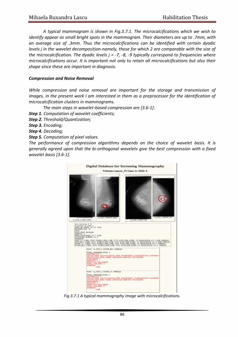
Mihaela Ruxandra Lascu Habilitation Thesis
86
A typical mammogram is shown in Fig.3.7.1. The microcalcifications which we wish to identify appear as small bright spots in the mammogram. Their diameters are up to .7mm, with an average size of .3mm. Thus the microcalcifications can be identified with certain dyadic levels j in the wavelet decomposition-namely, those for which 2 are comparable with the size of the microcalcification. The dyadic levels j = -7, -8, -9 typically correspond to frequencies where microcalcifications occur. It is important not only to retain all microcalcifications but also their shape since these are important in diagnosis.
Compression and Noise Removal While compression and noise removal are important for the storage and transmission of images, in the present work I am interested in them as a preprocessor for the identification of microcalcification clusters in mammograms.
The main steps in wavelet-based compression are [3.6-1]: Step 1. Computation of wavelet coefficients; Step 2. Threshold/Quantization; Step 3. Encoding; Step 4. Decoding; Step 5. Computation of pixel values. The performance of compression algorithms depends on the choice of wavelet basis. It is generally agreed upon that the bi-orthogonal wavelets give the best compression with a fixed wavelet basis [3.6-1].
Fig.3.7.1 A typical mammography image with microcalcifications.

Mihaela Ruxandra Lascu Habilitation Thesis
87
Algorithms for the Detection of Microcalcification Clusters
We shall propose a general strategy in constructing algorithms for extracting microcalcification clusters. We wish to distinguish between two types of algorithms. The first are autonomous [3.6-1] and do not involve a computer operator. The second are interactive and allow decisions to be made to improve parameter settings which depend on the image. Both approaches have the same major steps which I now describe. Step 1. Compression of the digitized image: an algorithm begins by utilizing compression as a preprocessor to the identification of the microcalcification clusters. The purpose of this step is to remove noise and still retain all microcalcifications. Step 2. Selecting only high frequency terms: the purpose of this step is to retain only those frequency terms that correspond to the size of the microcalcifications. Step 3. Reconstructing pixel values: this step constructs the image corresponding to the wavelet decomposition. Step 4. Nonlinear enhancement: the purpose of this step is to remove background and retain only the microcalcifications. Step 5. Threshold pixel values: this step thresholds pixel values to retain only the most intense. Step 6. Removing isolated pixels: this step is intended to remove any isolated hot pixels. A microcalcification should correspond to several hot pixels. Step 7. Filling out microcalcifications: the purpose of this step is to fill out microcalcifications. It could happen that the threshold in Step 5 removed pixels which correspond to microcalcifications and we want to restore these. Step 8. Finally, we want to test for clusters.
3.6.2 IMAGE PROCESSING TECHNIQUES
NI-IMAQ is a complete and robust application programming interface (API) for image acquisition. NI-IMAQ performs all the computer and board specific tasks for straightforward image acquisition without register-level programming. NI-IMAQ is compatible with NI-DAQ and all other National Instruments driver software for integrating imaging into any National Instruments solution. NI-IMAQ provides the interface path between LabVIEW, Measurement Studio and other programming environments and the hardware product. NI-IMAQ has both high-level and low-level functions for maximum flexibility and performance. High-level functions include single-shot and continuous-mode image acquisition. Low-level functions include imaging sequence setup. With only three icons, in LabVIEW it is possible to snap and display an image. You can build more complex configurations using this as a foundation. IMAQ Vision software from National Instruments adds high-level machine vision and image processing to LabVIEW, Measurement Studio and other programming environments. IMAQ Vision includes an extensive set of optimized functions for gray-scale, color and binary image display, image processing including statistics, filtering and geometric transforms, pattern matching, shape matching, blob analysis, gauging and measurement.
The possibilities and range for image processing and machine vision are numerous. To start with, in many applications you need a quantitative or statistical description of your image or region of interest. Statistical functions are calculated quickly. You can solve many inspection applications using simple functions such as average and standard deviation. Pattern matching functions are crucial in machine vision applications for locating features in the image.

Mihaela Ruxandra Lascu Habilitation Thesis
88
In Fig.3.7.2 the block diagram of the virtual instrument that implements the algorithm for the detection of microcalcification clusters is presented. Using this graphical program I obtained the images in Fig.3.7.3 and Fig.3.7.4 concerning mammographies with cancer.
The presented program is able to do the following: 1. Display initial image; 2. Smooth the image; 3. Highlight edges; 4. Thresholding the image; 5. Invert the image; 6. Fill holes in particles; 7. Remove border objects; 8. Filter particles; 9. Analyze particles.
Algorithm accuracy is very important. There is much to consider when choosing vision software – most important whether the software tools can correctly and accurately measure important part or object features down to the subpixel.
Fig.3.7.2. Block diagram for microcalcification clusters detection.
Fig.3.7.3. Abnormality 1 - Lesion type calcification
amorphous distribution regional. Fig.3.7.4. Abnormality 1,2,3 Lesion type
calcification punctuate-amorphous polymorphic distribution clustered.
If the software is not accurate and reliable, then it does not matter how fast your
computer is or how many pixels your camera has. Keep in mind that it is much easier to make accurate code faster than to make fast code more accurate. The NI Vision Development Module and Vision Builder AI include hundreds of accurate and reliable vision functions. The four most common machine vision application areas that have been used in my work are listed below, along with the most popular algorithms. 1. Enhancing an image – Use filtering tools to sharpen edges, remove noise or extract frequency information. Use image calibration tools to remove nonlinear and perspective errors

Mihaela Ruxandra Lascu Habilitation Thesis
89
caused by lens distortion and camera placement. One can also use the image calibration tools to apply real-world units to the measurements, so the tools return values in microns, millimeters or miles instead of pixels. 2. Checking for presence – This is the simplest type of vision inspection. To check for part or feature presence, one can use any of the color, pattern matching or histogram tools. A presence checks always results in a yes/no or pass/fail. 3. Locating features – Locating features is important when aligning objects or determining exact object placement, serving as a standard for all subsequent inspections. Edge detection, gray-scale pattern matching, shape matching, geometric matching and color pattern matching are all tools one can use to locate features. The tools return the object position (X, Y) and rotation angle down to one-tenth of a pixel. Geometric matching is immune to overlapping objects or objects that change in scale. 4. Measuring features – The most common reason to use a vision system is to take a measurement. Typically, one use edge detection, particle analysis and geometric function tools to measure distance, diameter, total count, angles and area. Whether you are calculating the total number of cells under a microscope or the angle between two brake-caliper edges, these tools always return a number instead of a location or pass/fail value. 5. Algorithm Performance – While accuracy and ease of use are often the two most important factors in choosing a vision system, execution speed is a third consideration. No matter how many hundreds of algorithms one have to choose from or how quickly one can build an application with them, if the inspection tools are inefficient and take too long to run, then much of the work goes to waste. NI vision software is highly optimized to squeeze performance from every possible source, resulting in software that rivals the fastest vision software package speed in the world. In fact, when compared to a leading vision software provider, NI vision software is consistently faster in many categories, as shown in Table 3.7.1 below:
Table 3.7.1 Vision software package speed.
NI Vision Software
Speed (ms)
Leading Vision
Software Speed (ms)
NI Speed Increase
Histogram 0.91 2.03 2.2X
Geometric Transform 3.1 10.3 3.3X
Morphology 1.8 5.9 3.3X
Geometric Matching 93.0 149.8 1.6X
Object Classifications 7.5 - -
After digitization, mammograms were automatically cropped to remove much of the
background (non-breast tissue) area. They were then manually processed to darken (digitally zero) pixels in regions that contained patient identifiers and were stored in files using a truly loss-less compression algorithm.
Another subtle issue is what elements of ground truth to count. That is, should an algorithm aim to find only proven cancers, all abnormalities suspicious enough to merit additional workup or some other criterion? Furthermore should a mass or microcalcification detection algorithm be evaluated using abnormalities of all types, or just ones that the algorithm was designed to detect?

Mihaela Ruxandra Lascu Habilitation Thesis
90
The method used to evaluate the algorithm was as follows. Each detection region was represented by the location of its maximum suspiciousness value. A detection region was scored as false positive if the pixel location of the abnormality fell outside all ground truth regions. A detection that fell inside a ground truth region counted as a true positive detection. In the event where multiple detections fell inside a ground truth region, one counted as a true positive detection and the others counted as false positive detections. This was decided because only one prompt is desired for each ground truth region. Any ground truth region that did not correspond to a detection location was counted as a false positive detection. Finally, all benign and malignant masses (microcalcifications) that were present in the ground truth were used for the performance evaluation.
3.7 COMPRESSION, NOISE REMOVAL AND COMPARISON IN DIGITAL MAMMOGRAPHY
In this chapter we are interested in compression and noise removal as a preprocessor for the identification of microcalcification clusters in mammograms. I propose a general strategy for constructing algorithms and implementing them in LabVIEW for compression, noise removal and extracting microcalcification clusters. The comparison method presented in this chapter aims to improve mammogram comparison by estimating the underlying geometric transformation for any mammogram sequence. It takes into consideration the various temporal changes that may occur between successive scans of the same woman and is designed to overcome the inconsistencies of mammogram image formation.
This work presents some characteristics of mammographic images since these will motivate the algorithms for microcalcification detection implemented in LabVIEW [3.7-1]. To count cancerous cells we use a common image processing technique called particle analysis, often referred to as blob analysis.
The evaluation of a CAD algorithm often begins with a retrospective evaluation of cancer cases. The reliable diagnosis of abnormalities from a single mammogram is an extremely difficult task even for a skilled radiologist and so it is increasingly the case that pairs of mammograms are compared [3.7-4]. These may be, for example, the left and right mammograms taken at the same session. Equally, when mammograms from an earlier time are available, the radiologist will routinely compare the older and more recent images. For this reason alone, the development of mammogram registration is increasingly important for the early detection of pathology. The potential clinical applications are as follows: 1) for women at high risk of developing breast cancer (e.g., women with family history of breast cancer or genetic susceptibility), usually have more frequent mammograms taken in order to detect a malignancy at as early a stage as possible. Previous (“normal”) mammograms are used as a baseline for comparison with recent ones. 2) for postmenopausal women who often decide themselves or are advised by their gynecologist physician to undergo hormone replacement therapy (HRT). However, there is a suggestion, based on clinical experience, that significant regional increases in tissue density could be an early indicator of breast cancer for women using HRT. For this reason it is important to be able to register HRT mammogram sequences, aiming at a more effective comparison for early detection of lesions. 3) for retrospective studies that aim to analyze temporal data in order to assess the accuracy and effectiveness of diagnosis in hospitals/screening centers. Such studies aim to define the rate of missed cancers and interval cancers, as well as to further educate clinicians in the important task of early diagnosis.

Mihaela Ruxandra Lascu Habilitation Thesis
91
Referring to Fig.3.7.1, the differences in imaging conditions and the temporal changes (5-year interval) render the comparison of A and B difficult, while by comparing B (recent mammogram) and C the physician can be reassured that the encircled region in B is scar tissue from the excision of a previous cancer in C (also encircled in the same location).
3.7.1 COMPRESSION AND NOISE REMOVAL
While compression [3.7-5] and noise removal are important for the storage and transmission of images, in the present work I am interested in them as a preprocessor for the identification of microcalcification clusters in mammograms. A schematic for wavelet-based compression is presented in Fig.3.7.2. The main steps in wavelet-based compression are [3.7-1]:
Fig.3.7.1. Typical mammography images with microcalcifications of the same woman (A and B) are
shown together with C, the registered version of A to B.
Fig.3.7.2. Wavelet based compression.
Step 1. Computation of wavelet coefficients; Step 2.Thresholding; Step 3. Encoding; Step 4. Decoding; Step 5. Computation of pixel values.
Wavelet Transform
Lossy
Thresholding
Reconstruction Decoding
Entropy Encoding
Lossless
Original
Image
Wavelet Representation
Wavelet Representation for Compressed
Image
Wavelet Representation for Compressed
Image Receiver Compressed
Image

Mihaela Ruxandra Lascu Habilitation Thesis
92
The inverse fast wavelet transform is used to compute the pixel values of the compressed image. This step takes again N operations. These are then the pixel values of the compressed image which is our approximation to the original image. In compression algorithms [3.7-5], [3.7-7] we have to take into account the choice of wavelet basis, the choice of metric and the level of compression.
3.7.2 IMAGE PROCESSING TECHNIQUES
The microcalcifications are represented by the connected pixels of ones and the background is represented by the zeros. By binarizing the image into ones and zeros, the task of writing image processing algorithms for microcalcification analysis is made easier. To find the area of a microcalcification, one have to count the pixels with values of one that are connected. Another benefit of binarizing the image for blob analysis is that the blob analysis calculations are fast. Many biomedical imaging applications can be solved using blob analysis, but also this kind of analysis is useful in industrial inspection applications.
The steps for counting cancerous cells are the following: Acquiring the image: configure the board for acquisition using a point-and-click user
interface; the configuration software saves the settings for the board to a configuration file, which is then used by the NI-IMAQ driver software in the development environment to simplify acquisition of images.
Thresholding to create a binary image: the threshold function segments an image into two regions, an object region (microcalcification) and a background region; in this process all pixels that fall within the gray-scale interval defined as the threshold interval are given the value one.; all other pixels in the image are set to zero; the result is a binary image that can be processed very rapidly; generally, algorithms to process binary images are faster than algorithms for gray-scale images.
Filtering to remove noise and particles on the border of the image: IMAQ function filters or removes the particles below a certain pixel size; another function removes the particles on the border of the image, because you cannot accurately determine the size of particles on the border of an image;
Microcalcifications (blob) analysis to count cells: IMAQ functions analyze blobs in an image; it is possible to count, label, measure cells and objects, calculate area, perimeter, orientation, location and other 49 parameters; there are many blob calculations such as area, perimeter, moment of inertia, orientation, mean chord, width, height, ellipse axis, elongation factor, circularity factor, type factor, projection, location, bounding rectangle; use morphology functions to erode, dilate, fill holes, convex (fill holes on the edges), reject objects on the border and separate blobs.
In Fig. 3.7.3a the block diagram of the LabVIEW virtual instrument for acquiring the mammography image is presented, while in Fig.3.7.3b the front panel of an acquired cancerous mammography is shown:

Mihaela Ruxandra Lascu Habilitation Thesis
93
a)
b)
Fig.3.7.3 a) LabVIEW block diagram for getting, creating and reading an image.
b) LabVIEW front panel for getting, creating and reading an image.
The following program I developed shows how to compute the histogram of an image or a region in the image. This program also shows how to set up and use the display tools to select and interactively work on different regions in the image. The results are presented in Fig.3.7.4.
Fig.3.7.4. LabVIEW front panel for the histogram of a region of interest (ROI) - one of the three
microcalcifications - in a mammography with three microcalcifications.

Mihaela Ruxandra Lascu Habilitation Thesis
94
The next developed program is intended to use the display tools in order to draw a line on the window that displays an image and get the pixel values of the image along that line (line profile) – Fig.3.7.5. One can typically use line profiles in inspection tasks to find the edges of an object or part being inspected.
Fig.3.7.5. LabVIEW front panel to inspect line profiles.
The blob analysis program I developed performs a series of gray scale filtering, threshold, binary morphology and particle analysis operations to measure the areas of all the large circular particles of the image – Fig.3.7.6 and Fig.3.7.7.
Fig.3.7.6.Filtered image with enhanced edge information.
a) b)
Fig.3.7.7 a) Original Image. b) Treshold image.

Mihaela Ruxandra Lascu Habilitation Thesis
95
3.7.3 MAMMOGRAPHY COMPARISON
Mammogram registration cannot usually be applied directly for the automatic detection of small abnormalities since the breast is a highly dynamic organ in which numerous normal changes occur regularly. This way, subtracting registered mammogram sequences may lead to a large number of false positives (in this context defined as normal changes and misregistrations) appearing in the difference image.
Mammogram registration could potentially be used to trace back “missed cancers” in previous mammogram sessions.
The novelty of the method I propose derives mainly from the detailed understanding of the temporal changes that can occur between successive acquisitions. Breast compression and imaging condition variability often lead to a nonrigid transform in the image plane (even a small difference in compression can lead to a significant and uneven displacement of the breast structures) and a nonrigid transformation image intensity, respectively. Temporal changes can also occur due to breast positioning, resulting in a rotation of the breast between two mammographic exposures.
The intensities of a mammogram pair can be normalized using the representation of interesting tissue [3.7-4] which results in the standard mammogram form (SMF), a standardized representation of a mammogram computed from the image intensities (film or digital) and imaging parameters of the system used to acquire the image. The method described in [3.7-4] deals with the geometrical alignment of mammogram sequences. This method incorporates a robust procedure to select consistent boundary landmarks for the automatic alignment of the breast boundary.
Fig. 3.7.8. Mammograms comparison using registrations.
(a) The original mammogram. (b) A random mammogram transform is applied and the mammogram is significantly deformed nonrigidly. (c) Mammogram is aligned to its original shape. (d) The difference image shows that the images are almost identical.
Fig.3.7.8 and Fig.3.7.9 enface the results provided by the program I developed for using pattern matching tools in IMAQ Vision for mammograms comparison. I used pattern matching in the following three general applications areas: Alignment - determine the position and orientation of a known microcalcification by locating features. We use the features as points of reference on the microcalcification; Gauging- measure lengths, diameters, angles and other critical dimensions concerning the microcalcifications; Inspection - detect simple flaws, such as missing parts.

Mihaela Ruxandra Lascu Habilitation Thesis
96
Fig.3.7.9. Mammogram sequences comparison.
3.8 A NOVEL MORPHOLOGICAL IMAGE SEGMENTATION WITH APPLICATION IN 3D ECHOGRAPHIC IMAGES
This chapter reviews ultrasound segmentation methods [3.8-1], [3.8-2] in a broad sense,
focusing on techniques developed for medical ultrasound images. Segmenting [3.8-8] abnormal from normal myocardium 3D real-time images using high-frequency intracardiac echocardiography (ICE) presents new challenges for image processing in LabVIEW. Gray-level intensity and texture features of myocardium ICE images with the same structural/perfusion properties substantially differ. There are significant limitation conflicts with the existing segmentation techniques. The novelty of this work consists of a new seeded region growing method to overcome the limitations of the existing segmentation techniques. The segmentation techniques [3.8-9], [3.8-10] are implemented using graphical programming LabVIEW and Vision. I use three criteria for region growing control: First, each voxel is merged into the globally closest region in the multifeature space. Second, structural similarity is introduced to overcome the problem that myocardial tissue, despite having the same property, may be segmented into several different regions using existing segmentation methods. Third, equal opportunity competence criterion is employed making results independent of processing order. This novel watershed segmentation method is applied to in vivo intracardiac ultrasound images using pathology as the reference method for the ground truth. The results demonstrate that this method is reliable and effective.
Three-dimensional echocardiography is a relatively new imaging modality and image analysis that is not yet well developed. Early work used either freehand ultrasound with 2-D image acquisition synchronized with recording the location of the slice with a position sensor,

Mihaela Ruxandra Lascu Habilitation Thesis
97
rotational 3-D probes, which acquired a sparse set of 2-D image sequences or real-time 3-D echocardiography based on the Volumetrics system [3.8-1], [3.8-2], [3.8-3].
However, a second generation of real-time 3-D echocardiography systems has recently been produced by Philips Medical Systems. This data is of higher quality than the rotational 3-D probe and Volumetrics systems [3.8-4]. One, therefore, has to take particular care in interpreting the results from early 3-D work as being representative of what it is possible to achieve today.
Ultrasound (US) image segmentation is strongly influenced by the quality of data. There are characteristic artefacts which make the segmentation task complicated, such as attenuation, speckle, shadows and signal dropout due to the orientation dependence of acquisition that can result in missing boundaries. Further complications arise as the contrast between areas of interest is often low. The scientific novelty of this work consists of a new seeded region growing method to overcome the limitations of the existing segmentation techniques. However, there have been recent advances in transducer design, spatial/temporal resolution, digital systems, portability, etc., that mean that the quality of information from an ultrasound device has significantly improved. This has led to increased use of ultrasound in not only its traditional area of application, diagnosis and CAD, but also in emerging areas such as image-guided interventions and therapy. Thus, there is currently a re-emergence of interest in understanding how to do one of the oldest image processing tasks, image segmentation applied to ultrasound data. As this work attempts to demonstrate that application of general image processing methods can suffice in the case of ultrasound data. Customized methods, which attempt to model the imaging physics in some way have proven to be more successful. This work focuses on techniques developed for native conventional B - mode ultrasound images and not segmentation of radio-frequency (RF) signal or Doppler images. Both two-dimensional (2-D) and three-dimensional (3-D) segmentation are considered, although the literature on 2-D methodology is far more extensive, reflecting the still relatively low but increasing use of 3-D image acquisition technology in clinical practice today. B-Mode ultrasound imaging collects the same information but adds a sense of direction where the echo is coming from a two-dimensional plane, as well as the memory to recall all the different echoes, strong and weak. This image becomes recognizable, particularly with practice. The recognizable image can then be evaluated for abnormalities and measured.
3.8.1 MORPHOLOGICAL SEGMENTATION
Morphological segmentation is a multiple-step process involving several NI Vision functions. The following list describes each morphological segmentation step. 1. The use of a global or local threshold to create a binary image. 2. If necessary, use binary morphology operations to improve the quality of the image by filling holes in particles or remove extraneous noise from the image. 3. Use the Danielsson function to transform the binary image into a grayscale distance map in which each particle pixel is assigned a gray-level value equal to its shortest Euclidean distance from the particle border. 4. Perform a watershed transform on the distance map to find the watershed separation lines. 5. Superimpose the watershed lines on the original image using an image mask.
Fig.3.8.1 summarizes the morphological segmentation process and shows an example of each step.

Mihaela Ruxandra Lascu Habilitation Thesis
98
In geography, a watershed is an area of land from which all rain that falls on the land flows into a specific body of water. In imaging, the watershed transform algorithm considers the objects under inspection to be the bodies of water. Fig. 3.8.2 illustrates this concept.
Figure3.8.2a shows an inspection image after it has been thresholded. Figure 3.8.2b shows the distance map of objects in the image using the gradient palette. Fig. 3.8.2c shows the topographic surface of the distance map. Each object from the inspection image forms a deep, conical lake called a catchment basin. The pixels to which the distance map function assigned the highest value represent the deepest parts of each catchment basin. The image background represents the land surrounding the catchment basins. To understand how a watershed transform works, imagine that the catchment basins are dry. If rain were to fall evenly across the image, the basins would fill up at the same rate. Eventually, the water in the basins represented by the circle and square would merge, forming one lake. To prevent the two lakes from becoming one, the watershed transform algorithm builds a dam, or watershed line, where the waters would begin to mix. Fig. 3.8.3a shows the same distance map as Fig. 3.8.2b with a line through the bottom two objects. Fig.3.8.3b shows the intensities of the pixels along the line in Fig.3.8.3a. Notice the watershed line preventing the waters from the two catchment basins from mixing.
Fig.3.8.1. Morphological segmentation process.

Mihaela Ruxandra Lascu Habilitation Thesis
99
Fig.3.8.2. 3D View of a Distance Map.
Fig.3.8.3. Watershed line.
As the rainfall continues, the rising water in all three lakes would begin to flood the land. The watershed transform algorithm builds dams on the land to prevent the flood waters from each lake from merging. Fig. 3.8.4 shows the watershed transform image after segmentation is complete. The water from each catchment basin is represented by a different pixel value. The black lines represent the watershed lines.
Echocardiography has been one of the driving application areas of medical ultrasound and the literature on methods for automatically segmenting and tracking the left ventricle (the normal chamber assessed for heart disease) is extensive.
Fig.3.8.4.Inspection image segmented with watershed lines.

Mihaela Ruxandra Lascu Habilitation Thesis
100
Most attention has been paid to tracking the motion of the endocardium (blood pool/tissue border) to allow for estimation of left ventricular areas/volumes and a derived measure, such as the ejection fraction, for regional wall motion assessment. In particular, these measures are used in diagnosis and assessment of ischaemic heart disease. Most analysis is based on 2-D acquisitions in which it is implicitly assumed that the principal component of motion is in the plane of the acquisition slice. The standard 2-D diagnostic views used for this are called the parasternal short-axis (SAX), and apical four-chamber (4C), two-chamber (2C) and three-chamber (3C) views. The latter three are also sometimes referred to as (apical) long-axis (LAX) views. The quality of data and hence challenges for segmentation, vary depending on the view due to the anisotropy of ultrasound image acquisition, artefacts such as shadowing from the lungs and attenuation which can be strong. Segmentation methods should also have strategies for avoiding the papillary muscles. Reliably finding the outer wall (often called epicardial border detection) is much more challenging, particularly from apical views. There are many papers on left ventricle tracking which deal with the tracking/deformation model independent of feature extraction or the imaging modality.
Watershed transform
The watershed transform is a powerful building block for morphological partitioning. In particular, a very powerful gray-scale segmentation methodology results from applying the watershed to the morphological gradient of an image to be segmented.
I shall focus only on the basic approach and leave more recent developments to the literature.
Let it be said that the watershed methodology has been highly developed so as to deal with numerous real-world contingencies and various implementation algorithms have been developed.
The watershed transform is the method of choice for image segmentation in the field of mathematical morphology. In gray scale mathematical morphology the watershed transform, originally proposed by Digabel and Lantuéjoul [3.8-5] and later improved by Beucher [3.8-6], is the method of choice for image segmentation.
Generally spoken, image segmentation is the process of isolating objects in the image from the background, i.e., partitioning the image into disjoint regions, such that each region is homogeneous with respect to some property, such as gray value or texture.
The watershed transform can be classified as a region-based segmentation approach. The intuitive idea underlying this method comes from geography: it is that of a landscape or topographic relief which is hooded by water, watersheds being the divide lines of the domains of attraction of rain falling over the region.
A watershed definition for the continuous case can be based on distance functions. Depending on the distance function used one may arrive at different definitions. Assume that the image f is an element of the space C(D) of real twice continuously differentiable functions on a connected domain D with only isolated critical points.
The power of the watershed transform is revealed when we can creatively design the input function and the marker. There are mainly three categories of input image: gradient, negate of the distance transform and the input image as it is. Next, I will explore the applications of the watershed when computed on the negation of the distance transform. The Voronoi diagram [3.8-7] is a partition of space into regions, each of which consisting of the points closer to one particular object than to any others. In morphology, the term “influence

Mihaela Ruxandra Lascu Habilitation Thesis
101
zone” is often used as a synonim of the Voronoi diagram. The Skeleton by Influence Zones (or SKIZ) is composed of the boundaries of the various influence zones. The watershed transform is a suitable method to compute the Voronoi diagram and the SKIZ. The idea is to compute the classical watershed transform of the distance transform for the background of the objects. The catchment basins are the Voronoi diagram and the watershed lines are the SKIZ. Voronoi diagrams have a surprising variety of uses: a) Nearest neighbor search -- For a query point q, finding its nearest neighbor from a fix set of points S is simply a matter of determining which cell in the Voronoi diagram of S contains q. b) Facility location -- This location is always at a vertex of the Voronoi diagram and it can be found in a linear-time search through all the Voronoi vertices. c) Largest empty circle -- A Voronoi vertex defines the center of the largest empty circle among the points. d) Path planning -- If the sites of S are the centers of obstacles we seek to avoid, the edges of the Voronoi diagram define the possible channels that maximize the distance to the obstacles.
Thus in planning paths among the sites, it will be safest to stick to the edges of the Voronoi diagram. We address the problem of binary image segmentation from the perspective of there being objects within the image that are touching or overlapping. This was one of the earliest application of the watershed. Our goal is to segment the single component in a manner consistent with the integrity of each of the two objects. A key to this problem and to many segmentation problems is to find markers for each of the two objects. 3.8.2 REAL TIME 3D IMAGE PROCESSING METHODOLOGY
The segmentation procedure for 3D echographic images is shown in Fig.3.8.5. The procedure is implemented in LabVIEW. Fig.3.8.6. shows the details of region growing controlled by criteria mentioned above.
Fig.3.8.5. Segmentation procedure for three dimensional biomedical images.
Criteria to obey
ICE Image
Texture analysis
Texture features
Region growing
Segmented results
Manual/Auto selection Seed regions
GCD&GS&EOC

Mihaela Ruxandra Lascu Habilitation Thesis
102
Fig.3.8.6. Flowchart of region growing circulation.
The following steps illustrate the LabVIEW and Vision implemented method VoxelSeg of segmenting objects. 1. Threshold—(Grayscale»Threshold) Threshold the image to isolate the objects we want to segment from the rest of the image. 2. Remove Noise—(Binary»Advanced Morphology or Binary»Particle Filter) Remove extraneous information from the binary image using various morphology operations. For example, we can fill in holes with the Advanced Morphology option Fill holes or remove noise with the Particle Filter function. 3. Create Distance Map—(Binary»Advanced Morphology) Use the Danielsson option to transform the binary image into a grayscale image in which the center of each object represents a local maximum in the image. If you were to look at the topographical surface of the image after applying the distance map, each object would appear as a smooth, gradual peak. 4. Apply Watershed Transform — (Grayscale»Watershed Segmentation) Apply the watershed transform to segment the image into local zones. A zone is determined by the watershed line that separates the influence zone of each peak.
Equal opportunity competence (EOC) criterion is used to make results independent of processing order. Only voxels at the edge of the seed regions at the beginning of a growing circulation are permitted to grow during the growing circulation. In Fig.3.8.7 the results for two watershed segmented echocardiography, with and without EOC criterion are presented.
In the past, dynamic cardiac 3D rendered images were possible by sequentially acquiring 2D images and then using a workstation to input 2D images for Cartesian coordinate conversion and volume rendering. Outside research settings, this time consuming process proved cumbersome and was simply impractical. Now that these technical and practical issues have been addressed, real-time 3D cardiac sonography has great potential to impact both patient care and throughput in a number of ways, including better pre- and post-surgical planning, improved measurement of heart function, decreased exam times and enhanced communication between clinicians and their patients. With real-time 3D cardiac ultrasound images, clinicians will be able to better quantify size, shape and function of the heart. However, the most
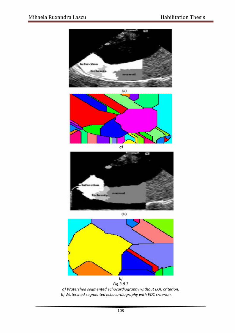
Mihaela Ruxandra Lascu Habilitation Thesis
103
a)
b)
Fig.3.8.7 a) Watershed segmented echocardiography without EOC criterion.
b) Watershed segmented echocardiography with EOC criterion.

Mihaela Ruxandra Lascu Habilitation Thesis
104
important contribution of real-time 3D sonography in cardiology may be improvement in locating abnormalities for surgical planning.
The new technology will also provide important information regarding surgical outcomes. A great benefit to obtain more diagnostic information and higher diagnostic confidence from real-time 3D cardiac ultrasound images is that it could lead to more rapid exam times and the reduction of patient wait times. Being able to see the whole heart makes examinations more simple and rapid, benefiting the staff and patient. The utility of this technology is unusually broad, as it is able to move beyond diagnostics into a key role in therapeutic procedures. As with any new technology, there will be a learning curve to understand 3D imaging. Even though the matrix transducer is somewhat larger than a standard 2D probe, the ergonomics are quite similar. The interface of the ultrasound unit is in general very user friendly. Because real-time 3D cardiac ultrasound involves looking at the heart as if you are holding it in your hands, with the additional ability to turn it any way you want, it is expect that the transition from 2D to 3D will be easily achieved and implemented.
I tested the method in images with seed regions placed in accordance to the pathology images. Ten images with infarcted myocardium were selected from diastolic frames in which both epicardial bead markers could be clearly seen. These images were acquired at the end of the ischemic period and during reperfusion. My goal was to segment ischemic viable, ischemic nonviable (infarcted), and normal myocardium. Myocardium was outlined by a specialist to simplify segmentation. Seed regions were manually selected by a cardiologist according to the gross pathology images. Myocardium in each intracardiac echocardiography (ICE) image was segmented using my new method.
The EOC criterion is very important in highlighting the infarcted zone. The shape and spatial distribution of segmented infarction and ischemic regions are close to the corresponding regions in the gross pathology images. It took approximately 40s for region growing with software programming in C++ language and approximately 10s for region growing with software programming in LabVIEW.
4. GRAPHICAL PROGRAMMING IN SOLAR, POWER ELECTRONICS AND MODERN EDUCATION
4.1 SOLAR RADIATION MODELING, MEASUREMENTS AND DATA PROCESSING
This work introduces the first station in Romania (Eastern Europe) [4.1-30], [4.1-32]
outfitted for systematic monitoring of solar irradiance on tilted surfaces. The resulted database is in many aspects unique for Romania, allowing for the first time to derive specific parameters like diffuse fraction or sunshine number. Also for the first time, the data collected on tilted surfaces can be used to test models reported in literature and to recommend the most fitting for the region, as detailed below.
The risk of climatic changes induced by CO2 emissions into the atmosphere (IPCC, 2007) has put urgency on renewable energy resources. Even if some primary resources can be used right away in thermal or mechanical systems, the main interest is for conversion into electricity, since electricity is the most flexible, all-purpose form of energy [4.1-13], [4.1-14], [4.1-15]. Annual growth rates reported by the photovoltaic industry (EPIA, 2009) indicate a boom in solar applications. Following the general trend, Romania [4.1-4] also experiences an increase of solar energy applications. One of the most exciting terrestrial photovoltaic applications [4.1-6] is the

Mihaela Ruxandra Lascu Habilitation Thesis
105
integration of solar modules into the roofs and facades of buildings, providing useful distributed power generation. Large scale solar architecture requires knowledge of collectable solar energy amount on surfaces with arbitrarily orientation in various places of the world [4.1-11], [4.1-18], [4.1-27]. Generally, solar radiation is a significant meteorological variable in a wide range of applications, from crop modeling to photovoltaic power plants [4.1-7]. Solar energy measurements have been carried out from the very beginning of solar converters operation in order to guide scientific and commercial applications. Accurate solar radiation measurements involve local and global networks. Like most countries, Romania set up a national network for monitoring global solar irradiation on horizontal surfaces, contributing to World Radiation Data Center located at the Main Geographical Observatory in St. Petersburg, Russia [4.1-1], [4.1-29].
However, compared to the needs, there is a low density of stations equipped for monitoring solar radiation. The use of the numerical models turns out to be the smart substitute to overcome the scarcity of recorded data [4.1-7], [4.1-8]. Additionally, even fewer stations worldwide are equipped for systematic measurements of solar components on inclined surfaces with arbitrarily azimuthally orientation. So far, in Romania, there are only sporadic, short-time series of data recordings on tilted surfaces, in most cases employing non-certified instruments and without public access to the data.
Four global solar irradiation models are tested against data measured during 2009 at the Solar Radiation Monitoring Station, located in Timișoara, Romania, in order to recommend the best fitting for the region [4.1-1], [4.1-9], [4.1-30], [4.1-32]. The quality of the collected data is evaluated in comparison with long term averaged data provided by the NASA Surface Solar Energy service. In this context, a new measurement has been inaugurated in 2008 as a joint project of research teams from “Politehnica” University Timișoara and the West University of Timișoara [4.1-20], [4.1-21], [4.1-22], [4.1-30], [4.1-32].
The next paragraphs report results after one year of successful operation of the first Romanian station outfitted for systematic monitoring of solar radiation on tilted surfaces, located at the West University of Timisoara, Romania. The aim is to give details about database content and utility in modeling solar irradiation over Romanian territory. New equations for calculating diffuse fraction and results of verifying models for estimation of total solar irradiation on tilted surfaces are reported [4.1-12]. Solar Instrumentation Calibrations and Measurements
Terrestrial solar radiation measurements are based on pyranometers that respond to radiation within a 2-pi steradian (hemispherical) field of view and/or pyrheliometers that are narrow field of view instruments (5.8° to 5.0°) measuring the nearly collimated (i.e., parallel rays) radiation from the 0.5° diameter solar disk and a small part of the sky. Hemispherical sky radiation can be measured by shading a pyranometer with a disk located to subtend the same angular field of view as a pyrheliometer.
The total hemispherical (sky + solar disk) radiation [4.1-2], [4.1-3], G, on a horizontal surface is the sum of the direct beam, B, projected on the surface (modified by the cosine of the incidence angle of the beam, i and sky radiation, D from the dome of the sky excluding the sun. These magnitudes are related by the equation G=B Cos(i)+ D. Examples of the instrumentation [4.1-5], [4.1-28], [4.1-31] are shown in Fig. 4.1.1.
The theoretical relationship shows that measurement of any two of the radiation quantities allows computation of the third. This component equation is the basis of the outdoor

Mihaela Ruxandra Lascu Habilitation Thesis
106
calibration of radiometers. Namely, many pyranometers can be simultaneously calibrated using direct beam and sky diffuse measurements with highly specialized and well-characterized reference pyrheliometers and pyranometers.
Fig.4.1.1. Instruments for measuring solar radiation components.
In the next section a short description of the experimental setup is presented and the main characteristics of the database are summarized.
4.1.1 EXPERIMENTAL SETUP AND DATABASE
The Solar Radiation Monitoring Station (SRMS) is located at geographical coordinates
45°46´N, 21°25´E and 85 m altitude. DeltaOHM LP PYRA 02 [4.1-5] and LP PYRA 12, First Class pyranometers in accordance with ISO 9060 standard are fulfilling the requirements defined by the World Meteorological Organization. LP PYRA 02 pyranometer is based on a thermopile sensor with a typical sensitivity of 10μV/(Wm2). Because of the shadow ring, LP PYRA 12 measures the diffuse solar irradiance eliminating the contribution of direct irradiance. Besides the direct radiation the shadow-ring intercepts part of the diffuse light. In order to get the real value of the diffuse irradiance, the measured values are multiplied by the correction coefficients
provided by the manufacturer in the instrument manual (DeltaOHM, 2010)[4.1-5]. The main meteorological parameters: temperature, air pressure, relative humidity and
windspeed are also recorded in standard conditions. The sensors are integrated into an acquisition data system based on a National Instruments PXI Platform consisting of a PXI-8105 controller and PXI-6259 data acquisition board optimized for high accuracy (NI, 2010 ) [4.1-17]. The system operation is relying on a LabVIEW application. Measurements of all parameters, meteorological, actinometrical and electrical, are simultaneously performed all day long at constant time intervals of 15 seconds. The PXI controller clock deviates less than 15 seconds per month. In order to maintain the clock accuracy the clock is manually adjusted two times per month. The monitored parameters on the SRMS platform [4.1-25] are: global, diffuse and reflected solar irradiance components on horizontal surface along with the total solar irradiances on other four directions: 45° inclination facing South and South-West and vertical wall facing South and South-West.
Instantaneous values of monitored parameters are displayed online (SRMS, 2010) [4.1-25]. Starting with January 1, 2009, series of hourly data packaged in monthly files are available for free use in research and education. The systematic series of data recorded on tilted

Mihaela Ruxandra Lascu Habilitation Thesis
107
surfaces and the high recording rate are the major features of the database which make it unique in Romania.
4.1.2 SOLAR IRRADIATION COMPONENTS
Long-term recordings of solar irradiance in the grid of the Romanian National
Meteorological Agency are recorded every three hours. As mentioned, on the SRMS platform the data is recorded at 4 samples per minute. Thus, the number of measurement points per day varies between 2050 in winter and 3750 in summer, for every channel. Fig. 4.2.1 depicts the sunshine number recorded on June 9, 2009 on the SRMS Platform. The curves are in fact constructed from so many discrete points that they appear continuous. This is to highlight a benefit resulted from the high frequency of data recording. However, the main advantage of such high recording rate comes from the first issue: it allows high accuracy in calculating solar irradiation. A visual inspection shows that even if the solar irradiance varies sharply, there are enough points to perform an accurate integral (by summing up), in order to obtain the corresponding irradiation components.
Fig. 4.2.1. Global G(0) and diffuse Gd(0) solar irradiance on June 9, 2009, in Timisoara. Sunshine number ξ
is also displayed.
Table 4.2.1 summarizes monthly mean of daily irradiation computed from solar irradiance data recorded in 2009 on SRMS platform. Table 4.2.1. Monthly mean of daily global 𝑔and diffuse 𝑑 solar irradiation incident on a horizontal
surface and total 45 solar irradiation incident on a surface sloped with 45° facing South, calculated using data recorded in 2009 on SRMS platform.
In this work, results after one year operation of the first Romanian station equipped for solar radiation monitoring on tilted surfaces are reported. Various hourly integrated solar radiation data along with meteorological parameters are available online [4.1-16] [4.1-23], [4.1-24], [4.1-25],[4.1-26].
The data provide the opportunity to derive specific solar radiation models as well as to verify and calibrate models proposed by others. It is illustrated by reporting a new diffuse
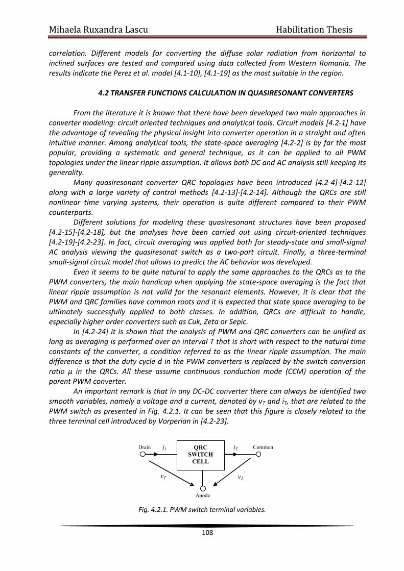
Mihaela Ruxandra Lascu Habilitation Thesis
108
correlation. Different models for converting the diffuse solar radiation from horizontal to inclined surfaces are tested and compared using data collected from Western Romania. The results indicate the Perez et al. model [4.1-10], [4.1-19] as the most suitable in the region.
4.2 TRANSFER FUNCTIONS CALCULATION IN QUASIRESONANT CONVERTERS
From the literature it is known that there have been developed two main approaches in
converter modeling: circuit oriented techniques and analytical tools. Circuit models [4.2-1] have the advantage of revealing the physical insight into converter operation in a straight and often intuitive manner. Among analytical tools, the state-space averaging [4.2-2] is by far the most popular, providing a systematic and general technique, as it can be applied to all PWM topologies under the linear ripple assumption. It allows both DC and AC analysis still keeping its generality.
Many quasiresonant converter QRC topologies have been introduced [4.2-4]-[4.2-12] along with a large variety of control methods [4.2-13]-[4.2-14]. Although the QRCs are still nonlinear time varying systems, their operation is quite different compared to their PWM counterparts.
Different solutions for modeling these quasiresonant structures have been proposed [4.2-15]-[4.2-18], but the analyses have been carried out using circuit-oriented techniques [4.2-19]-[4.2-23]. In fact, circuit averaging was applied both for steady-state and small-signal AC analysis viewing the quasiresonat switch as a two-port circuit. Finally, a three-terminal small-signal circuit model that allows to predict the AC behavior was developed.
Even it seems to be quite natural to apply the same approaches to the QRCs as to the PWM converters, the main handicap when applying the state-space averaging is the fact that linear ripple assumption is not valid for the resonant elements. However, it is clear that the PWM and QRC families have common roots and it is expected that state space averaging to be ultimately successfully applied to both classes. In addition, QRCs are difficult to handle, especially higher order converters such as Cuk, Zeta or Sepic.
In [4.2-24] it is shown that the analysis of PWM and QRC converters can be unified as long as averaging is performed over an interval T that is short with respect to the natural time constants of the converter, a condition referred to as the linear ripple assumption. The main difference is that the duty cycle d in the PWM converters is replaced by the switch conversion ratio μ in the QRCs. All these assume continuous conduction mode (CCM) operation of the parent PWM converter.
An important remark is that in any DC-DC converter there can always be identified two smooth variables, namely a voltage and a current, denoted by vT and iT, that are related to the PWM switch as presented in Fig. 4.2.1. It can be seen that this figure is closely related to the three terminal cell introduced by Vorperian in [4.2-23].
Fig. 4.2.1. PWM switch terminal variables.
QRC
SWITCH CELL
Drain Common
Anode
vT
v2
iT i1

Mihaela Ruxandra Lascu Habilitation Thesis
109
The switch cell conversion ratio is defined as:
T
2
v
v (4.2.1)
All the variables are considered to be averaged, but for the sake of simplicity the averaging symbol will be omitted. Because in an averaged model the steady state variables become constant, capitals will denote the steady-state values, except for switch conversion ratio μ and the switching frequency fs, for which the symbols μ0 and fs0 will be used, respectively. Hatted variables will denote the small signal perturbations. 4.2.1 PROPOSED STATE-SPACE MODEL All above considerations suggest that many properties inherited from the parent PWM converter can be used together with the peculiar properties of the QRCs. Indeed, what differs in a QRC converter compared to its PWM counterpart is the value of the switch conversion ratio μ. Obviously, in a PWM converter we have μ=d, while in a QRC it has been shown [4.2-25], [4.2-26] that μ has a nonlinear dependency on vT and iT and a linear dependency on the switching frequency fs:
)i,v,f( TTs (4.2.2)
Therefore a QRC converter can be viewed as a system according to the block diagram presented in Fig. 4.2.2. Linearizing (4.2.2) results in:
TiTvsc iKvKfKˆ (4.2.3)
where
0s
0
0sc
ffK
(4.2.4)
0Tv
VK
(4.2.5)
0Ti
IK
(4.2.6)
After linearization of the power converter and control, the linearized system takes the
form illustrated in Fig. 4.2.3.
The overall system exhibits two inputs, sf and gv and one output, ov . Our goal is to
find two transfer functions. The transfer function relating the supply variable gv and the output
ov is known as audiosusceptibility:
)s(v
)s(v)s(H
g
og (4.2.7)
The second transfer function, called control to output, relates the control variable sf and the
output ov :
)s(f
)s(v)s(H
s
oc (4.2.8)

Mihaela Ruxandra Lascu Habilitation Thesis
110
Fig. 4.2.2. System representation of a QRC converter.
Figure 4.2.3. The linearized model of a QRC converter.
The key of the method is to observe that a transfer function between any variable in the power converter and can be derived from the PWM parent converter as the transfer function
between that variable and d , in which D is replaced by μ0 and d by . Then, if properly
chosen, as it will be shown in the next paragraph, these transfer functions can be combined with (4.2.3) to provide the desired results. Moreover, the transfer functions in the power converter can be calculated in vector form using the state space matrices. The calculations are even simpler because vT and iT are in fact state variables or combinations of state variables. 4.2.2 TRANSFER FUNCTIONS DERIVATION A. Scalar transfer functions derivation
In order to derive the audiosusceptibility and control to output transfer functions we shall begin
by expressing Tv , Ti and ov in terms of the intrinsic converter inputs and gv :
gvvvT vHˆHvgTT (4.2.9)
gviiT vHˆHigTT (4.2.10)
gvvvo vGˆGvgoo (4.2.11)
where TvH ,
gTvvH , TiH ,
gTviH , ov
G , govvG are the transfer functions between the indexed
variables when the other input is not perturbed. For example, 0v
Tv
g
T ˆ
vH
, etc. Note that
ovG and
govvG are the classical transfer functions in a PWM converter with d . Now
replacing Tv from (4.2.9) and Ti from (4.2.10) in (4.2.3) one obtains:
scgviiiigvvvvv fKvHKˆHKvHKˆHKˆgTTgTT
(4.2.12)
From (4.2.12) can be expressed as:
POWER CONVERTER
CONTROL
vg vo
fs
vT iT μ
POWER
CONVERTER
Ki
Kc
KV
gv ov
sf
Tv Ti
+ +
+

Mihaela Ruxandra Lascu Habilitation Thesis
111
sivv
Cg
iivv
viivvvf
KHK1
Kv
HKHK1
HKHKˆ
TTTT
gTgT
(4.2.13)
Substituting from (4.2.13) in (4.2.11), after some simple algebra, a relationship relating ov
to gv and sf is obtained in the form:
sivv
vcg
iivv
viivvvv
vv0 fKHK1
GKv
HKHK1
)HKHK(GGv
TT
0
TT
gTgT0
g0
(4.2.14)
From (4.2.14) the desired audiosusceptibiliy and control to output transfer functions can be
easily identified as:
TT
gTgT0
g0iivv
viivvvv
vvgHKHK1
)HKHK(GG)s(H
(4.2.15)
TT
0
iivv
vcc
HKHK1
GK)s(H
(4.2.16)
B. Transfer functions representation in matrix form
As known, we can describe the CCM operation of the PWM parent converter using a state-space approach. Let x be the state vector, ]v[u g the input vector and y the state vector. Defining
the output vector y as:
tTTo ivvy (4.2.17)
let A1, B1, E1, F1 and A2, B2, E2, F2 be the classical state matrices corresponding to the two topological PWM states (index 1 is correlated to the ON state of the transistor). Note that as vT and iT are in fact state variables or linear combinations of state variables, then the elements of E1, F1, E2 and F2 will be practically only 0 and 1 and therefore these matrices are very easy to be calculated. Let also )s(Gg be the matrix audiosusceptibility and )s(Gc the control to output
transfer function with respect to , both in the QRC converter. It is known [4.2-2] that )(sGg
and )s(Gc can be written from the PWM parent converter with d :
FB)AsI(E)s(G 1g (4.2.18)
1c )AsI(E)s(G (4.2.19)
where I is the unity matrix of converter order and
U)2B1B(X)AA( 21 (4.2.20)
U)FF(X)EE( 2121 (4.2.21)
UBAX 1 (4.2.22)
21 A)1(AA (4.2.23)
21 B)1(BB (4.2.24)
21 E)1(EE (4.2.25)
21 F)1(FF (4.2.26)
]V[U g (4.2.27)
Due to the classical definition of the small-signal transfer functions, we have

Mihaela Ruxandra Lascu Habilitation Thesis
112
)s(ˆ)s(G)s(v)s(G)s(y cgg . As the first component in y is ov , the second is Tv and the
third is Ti and because )s(Gg relates )s(y to )s(vg , then )s(Gg will be of the form
gT
gT
g0
vi
vv
vv
g
H
H
G
)s(G . Similarly, the form of )s(Gc will be
T
T
0
i
v
v
c
H
H
G
)s(G . Therefore the scalar
transfer functions govvG ,
gTvvH , gTvi
H , ovG , Tv
H , TiH can be briefly written as:
)1(GG gvv g0 (4.2.28)
)2(GH gvv gT (4.2.29)
)3(GH gvi gT (4.2.30)
)1(GG cv0 (4.2.31)
)2(GH cvT (4.2.32)
)3(GH ciT (4.2.33)
Using (4.2.28) to (4.2.33) in (4.2.15) and (4.2.16), the final relationships for audiosusceptibility
and control to output transfer functions are found in the final form:
)3(GK)2(GK1
)]3(GK)2(GK)[1(G)1(G)s(H
cicv
gigvcgg
(4.2.34)
)3(GK)2(GK1
)1(GK)s(H
cicv
cvc
(4.2.35)
In order to calculate the desired transfer functions one has to use (4.2.27) to (4.2.18) exactly in
this reversed order and then (4.2.34) and (4.2.35). Note that these relationships apply to any
converter and therefore are general. What differ from one topology to another are:
a. Expressions of vT and iT as a function of state variables, thus affecting matrices E1, F1, E2 and F2.
b. Matrices A1, B1, A2, B2 that change from one converter to another. c. Order of matrix I, according to converter order.
4.2.3 VERIFICATION AND APPLICATIONS OF THE PROPOSED METHOD
The proposed method was verified in deriving the transfer functions parameters for the classical ideal buck, boost and buck-boost QRC converters. The results were compared to those obtained in [4.2-24]. The synthetic table provided in [4.2-24] is reproduced in Table I. In order to verify the proposed technique, we shall derive the audiosusceptibility and the control to output transfer functions for a buck converter and we shall compare the results to those in Table 4.2.1. The method was implemented in Matlab using Symbolic Math Toolbox. For the buck QRC

Mihaela Ruxandra Lascu Habilitation Thesis
113
Buck Boost Buck-Boost 0TV 0Vg 0V 00 VVg
ogG RVKVKμTi
Tv
0
00
1
RKVμKVμ
RμKVμ
iTνT
iT
0'00
2'0
2'0
0'0
2
1
R
KVμKVμ
RμKVμμμKVμ
iTνT
iTνT
0'00
2'0
'0
02'
00
'00
'0
2
ocG RVK
VKTi
Tc
0
0
1
RKVμKVμ
KVμiT
νT
cT0'
002'
0
0'0
2
R
μKVμKVμ
KVμiT
νT
cT00'
002'
0
0'0
1
pω RVKω Ti
F01
RKVμKVμω iT
νTF0'
002'
02
R
μKVμKVμω iTνTF
00'00
2'0
1
Q
F
TiF
Ti
RVK
RR
RVK
0
01
F
iTνTF
iTνT
RKV
μKV
RR
RKVμKVμ
0'0
0
0'00
2'0
1
2
F
iTνTF
iTνT
RKV
μμKV
RR
RμKVμKVμ
0'0
00
00'00
2'0
1
1
zcω ∞ FLRμ 2'
0 0
2'0
μLRμ
F
zgω ∞ ∞ FνT
iTνT
LKVμ
RKVμμμKVμRμ
00
02'
00
'00
'0
'0
2011
1
pp
zgggν
ωs
ωs
Q
ωs
GsG 2011
1
pp
zcccν
ωs
ωs
Q
ωs
GsG FFF
CLω 1
F
FF C
LR
converter we have gT vv and LT ii . Consequently, the state matrices are:
Table 4.2.1. Converter transfer functions parameters as calculated in [4.2-24]
12122121111 FF;EE;0
0B;AA;
0
1
0
F;
01
00
10
E;0L
1B;
RC
1
C
1L
10
A
(4.2.36)
The Matlab program for calculating the transfer functions parameters is presented below.
clear all; close all; clc;
% Buck converter
syms s Kv Ki Kc Vg L C R u0
I=eye(2); % unity matrix of converter order
U=[Vg];
A1=[0 -1/L;1/C -1/(R*C)];
B1=[1/L; 0]; E1=[0 1;0 0;1 0]; F1=[0; 1; 0];
A2=A1; B2=[0; 0]; E2=E1; F2=F1;
Au=u0*A1+(1-u0)*A2; Bu=u0*B1+(1-u0)*B2;
Eu=u0*E1+(1-u0)*E2; Fu=u0*F1+(1-u0)*F2;

Mihaela Ruxandra Lascu Habilitation Thesis
114
X=-inv(Au)*Bu*U;
csiu=(A1-A2)*X+(B1-B2)*U;
zetau=(E1-E2)*X+(F1-F2)*U;
Gg=Eu*inv(s*I-Au)*Bu+Fu; Gg=simple(Gg);
Gc=Eu*inv(s*I-Au)*csiu+zetau; Gc=simple(Gc);
Hg=Gg(1)+(Gc(1)*(Kv*Gg(2)+Ki*Gg(3)))/(1-Kv*Gc(2) -Ki*Gc(3));
Hgbuck=simple(Hg),
Hc=(Kc*Gc(1))/(1-Kv*Gc(2)-Ki*Gc(3));
Hcbuck=simple(Hc).
After running it the following results are obtained:
2p
2
p
g0gs
Q
s1
1H)s(H
(4.2.37)
2p
2
p
c0cs
Q
s1
1H)s(H
(4.2.38)
where the values of the parameters are listed in Table 4.2.2.
Table 4.2.2. Buck transfer functions parameters calculated according to the proposed method
Parameter Value Parameter Value
0TV gV p R
VK1 0Ti
F
ogH
R
VK1
VK
0Ti
0Tv0
Q
F
0TiF
0Ti
R
VK
R
RR
VK1
ocH
R
VK1
VK
0Ti
0Tc
F
FFCL
1
FR F
F
C
L
The differences between Table 4.2.1. and Table 4.2.2. are given by the fact that in
[4.2-24] was defined as TiTvsc iKvKfKˆ , that compared to (4.2.3) reveals there is a
minus sign related to iK . Also some notations differ, namely Gog and Goc in [4.2-24] are Hog and
Hoc in the present paper. One can easily see that making ii KK in Table 4.2.2. perfect match
with the parameters in Table 4.2.1 for the buck converter is obtained. This confirms the validity of the proposed method.

Mihaela Ruxandra Lascu Habilitation Thesis
115
Finally, let us represent the control to output transfer function both for a PWM and for a ZCS QRC full wave (FW) buck converter that performs the same conversion, from 48V to 23.12V. The resonant elements are: H4L , nF147C . The switching frequency is
kHz100fs . The output inductor and the output capacitor are 10mH and 100μF, respectively.
The corresponding Matlab program is provided below and the results are presented in Fig. 4.2.4. It can be seen that in the QRC case there is a loss of gain compared to the PWM case, while the phase is practically the same and because of this the traces are overimposed and only one trace can be seen.
% PWM and ZCS FW QRC buck converter small-signal transfer functions
clear all; close all; clc;
% Buck ZCS QRC FW;
Vg=48; R=12; L=4e-6; C=147e-9; fs=100e3; LF=10e-3; CF=100e-6;
VT0=Vg;
f0=1/(2*pi*sqrt(L*C));
F=fs/f0;
miu0=F;
Kv=0; Ki=0; Kc=1/f0;
wF=1/sqrt(LF*CF); RF=sqrt(LF/CF);
G0c=VT0*Kc/(1-Ki*VT0/R);
wP=wF*sqrt(1-Ki*VT0/R);
Q=sqrt(1-Ki*VT0/R)/(RF/R-Ki*VT0/RF);
Gc=tf([G0c],[1/wP^2 1/(wP*Q) 1]);
bode(Gc,’k’); hold on
% Buck PWM;
D=miu0;
Q=R/sqrt(LF/CF); w0=1/sqrt(LF*CF);
NUM=Vg; DEN=[1/w0^2 1/(w0*Q) 1]
Gcpwm=tf(NUM,DEN)
bode(Gcpwm,'k.');
title('Control to output transfer function for a buck ZCS QRC FW (blue) and a buck PWM (red)
converter')

Mihaela Ruxandra Lascu Habilitation Thesis
116
Figure.4.2.4. Control to output transfer function representation in QRC (solid) and PWM (dotted) case.
4.3. E-LEARNING PRACTICAL TEACHING OF UNCONTROLLED RECTIFIERS
Efficient learning in engineering assumes a mixture between theory and practical work. The drawback of a pure theoretical approach in a curriculum is that less attention is paid to the phenomena looming around laboratory experiments and real components. The results of this, corroborated with the rapid development of computer simulations, were that hands-on laboratory experience was vanishing and that computer simulations gained more and more attention. However, it is of crucial importance for the student to gain practical experience. Physical experiments help the students in practical testing and allow them to see the influence of second and higher order effects or parasitics that are often difficult to simulate as in reality. Hence it is of great importance to give the student a real world experience. Although classical hands-on laboratories are very useful, they may have limitations regarding space, time and staff costs. These problems can be significantly alleviated by using remote experiments and remote laboratories when the students operate with real systems, although they are not present in the laboratory. The proliferation of web based distance education courses in recent years involves new challenges for teaching disciplines involving a high level of practical work. For engineering related distance education the use of a web-based delivery mechanism is the only realistic method of providing hands-on experience, allowing remotely located students to complete laboratory assignments, unconstrained by time or geographical considerations, while developing skills in the use of real systems. In this way access to the experiments is available 24 hours a day, giving the users the possibility to access the laboratory when they most need it,
-150
-100
-50
0
50M
agnitu
de (
dB
)
101
102
103
104
-180
-135
-90
-45
0
Phase (
deg)
Control to output transfer function for a buck ZCS QRC FW (blue) and a buck PWM (red) converter
Frequency (Hz)

Mihaela Ruxandra Lascu Habilitation Thesis
117
sitting comfortable in a remote location. They can change parameters, perform experiments, observe results in graphical or numeric view and download them. In addition, a booking system allows the remote users to plan their time and experiments. 4.3.1 LEONARDO DA VINCI PROJECT AND ITS PHILOSOPHY
The Leonardo da Vinci project with the acronym EDIPE (E-learning Distance Interactive Practical Education) is approved to create a full set of distance experiments called PEMCWebLab in an integrated learning platform, providing the user with a practical experience in Power Electronics and Electrical Drives education. They are real experiments conducted in the laboratory but remotely accessed, controlled and monitored by web-based tools. The participants are twelve universities with the span across the EU. The expected results are: • Elaboration of clear learning objectives for distance experimental education, • Guidelines for project oriented measurements, • Synthesis oriented experimental work, • Technology and technical documentation for distance practical education and measurements via Internet, • Different experiments, each with its own specificity. The outputs from the project are: • Teaching material: guidelines, manuals, documentation in English and other languages, • Distance and virtual laboratories approaches via web, • Measurement results and reports obtained via Internet.
Each experiment has its own server because it is located in a different location. Remote users first log onto a main booking server, located at the University of Maribor, after which they will be directed to the specific server for actually performing the experiment into a separate individual page. The booking system is based on the Moodle course management system (www.moodle.org). Moodle is a widely adopted software package for producing Internet-based courses and websites. In addition to the original booking system, some modifications have been made [4.3-1], enabling easy booking creation for those remote experiments that were developed under the LabVIEW Web Publishing Tools. The layout of Moodle pages for all experiments is uniform. The users are divided in two groups: authorized users and guests. Only authorized users can control the experiment. The guests can only observe measured values and waveforms but they have no control of any part of the system. The learning issues addressed in the PEMCWebLab integrated learning platform are: • Learning objectives; • Education; • Animation and Simulation; • Experiment. The order of these issues is important. For safety reasons no student is allowed to perform any experiment until he or she has proofed adequate knowledge of the requested experiment. First the learning objectives are defined, while a theoretical background of each individual experiment is given in part Education. Interactive animation and/or Simulation are the steps preceding the real Experiment.
After completion of the real experiment the students are given a questionnaire and have to submit their report for the final evaluation. All learning procedures are recorded for future reference and analysis.

Mihaela Ruxandra Lascu Habilitation Thesis
118
Teacher oriented and student oriented education
Many teachers continue to think their main duty is to transfer their knowledge to the students by giving lectures or by organizing laboratory experiments. In this view, the accent is on teaching, rather on learning [4.3-2], [4.3-3]. Presently, the new philosophy assumes that knowledge is not transferred, but that the learner himself constructs knowledge on the basis of prior knowledge and additionally acquired information. “Learning by doing” or “Learning by experimenting” approaches are accompanied by an output oriented curricula as part of the shift emphasis from teaching to learning. This view is referred to as constructivism while in the teaching-oriented approach the student is rather passive, in the vision of learning-oriented approach the student plays an active role, constructing knowledge on the basis of prior knowledge and additionally acquired information, with teaching as a facilitating precondition. In this spirit, the PEMC WebLab experiments are oriented not only to analysis but also to synthesis. They include design aspects and the measurements are thought as a project with clear targets. The learning process in power electronics includes all important steps: general theory, key design factors (device stresses, ripple estimation, power quality aspects, etc.), simulation and real experiment measurements [4.3-4].
In this thesis the module “Single Phase and Three Phase Rectifier Circuits” will be discussed in detail.
General architecture
The structure of the distance laboratory is shown in Fig. 4.3.1 in the situation when the chosen module is “Single Phase and Three Phase Rectifier Circuits” [4.3-5]. For the booking operation Moodle was chosen and the local server uses LabVIEW [4.3-6], [4.3-7] for controlling the experiment. The Web Publishing Tools that come with LabVIEW [4.3-7] are used both for interfacing and remote controlling the experiment, namely to choose the rectifier type, select the desired waveforms and perform different measurements. The proposed hardware solution depicted in Fig. 4.3.2 is based on ELWE teaching module as it offers good modularity and simple connectivity. The PCI-MIO-16E-1 DAQ card together with the SCB-68 shielded I/O connector block for DAQ devices are used for acquisition and measurements. The Switching Board Interface (SBI) is controlled from LabVIEW and its purpose is to configure the desired rectifier topology and to select the signals for data acquisition. Functionally, it consists of a 32 bit shift register followed by buffers that switch a relay matrix on and off.
LabVIEW based Control of a Switching Board for Distance E-learning
The purpose of this paragraph is to present in detail how the Switching Board Interface is built and how it is controlled from LabVIEW. This is absolutely necessary in configuring the desired rectifier topology and for data acquisition. The block diagram of the Switching Board Interface is shown in Fig. 4.3.3. As the National Instruments PCI-MIO-16E-1 acquisition board is
used, the three inputs 1I , 2I and 3I in the register area are connected to the digital outputs 1O ,
2O and 3O of the acquisition board respectively. The registers are 8-bit serial-in parallel-out
D-type SN74HC594 [4.3-8] shift registers. The serial 'HQ output is shown in Fig. 4.3.4 and is used

Mihaela Ruxandra Lascu Habilitation Thesis
119
PCI-MIO-16E-1 DAQ
Board
SCB-68
Shielded I/O
Connector
Block for
DAQ Devices
Switching
board
interface
Uncontrolled
rectifier
experiment
Internet
Users
Moodle
booking
system
Measuring server
Fig.4.3.1. Structure of the distance laboratory for E-learning practical teaching of uncontrolled rectifiers.
LabVIEW 8.0
Web
Publishing
Tools
SWITCHING BOARD
INTERFACE
45Vrms/phase6 PHASE TRANSFORMER
3 x 1Ω
CURRENT SENSING
RECTIFIER SECTION
SCB-68Shielded I/O Connector Block for
DAQ Devices
100Ω
25Ω
2 x 470μF
50mH
LOAD SECTION
PCI-MIO-16E-1 DAQ Board
SWITCHING BOARD
INTERFACE
45Vrms/phase6 PHASE TRANSFORMER
3 x 1Ω
CURRENT SENSING
3 x 1Ω3 x 1Ω
CURRENT SENSINGCURRENT SENSING
RECTIFIER SECTIONRECTIFIER SECTION
SCB-68Shielded I/O Connector Block for
DAQ Devices
100Ω
25Ω
2 x 470μF
50mH
LOAD SECTION
PCI-MIO-16E-1 DAQ Board
Fig. 4.3.2. Hardware architecture of the “Single Phase and Three Phase Rectifier Circuits”.

Mihaela Ruxandra Lascu Habilitation Thesis
120
for cascading four such registers, finally resulting in a 32-bit output word. The storage clock
SRCLK of each register is connected to the digital output 1O of the acquisition board, while
output 2O is connected to each shift register clock RCLK input. Both clocks are positive edge
triggered. Serial input data is provided by the digital output 3O . The parallel outputs of the
registers form a 32-bit word, each bit addressing a relay in the relay matrix. For buffering purposes, four ULN2804 high-voltage high-current Darlington arrays are
used, allowing up to 500 mA for driving the inductor coil of the relay. The relays are used both to obtain the desired rectifier configuration and to provide the signals of interest to the acquisition board. They are also used to switch on and off the input voltages provided by the three phase transformer.
For ensuring safe operation for the acquisition board and for the power devices, the order the relays are switched is important. At the beginning of each experiment all the relays are assumed to be in the off state from the exit sequence of the previous experiment. This means that the sinusoidal power supplies are disconnected and so the next relays switchings will take place without current flowing through them. Because of the inductive nature of the load a “temporary freewheel diode” (TFD) is used during experiment configuration. The first relay that is switched on is that corresponding to the TFD and as a consequence the TFD is connected in antiparallel to the load. The next set of relays that are simultaneously switched on are those for configuring the rectifier and the load. This is achieved writing a 32-bit word in the shift registers. Next, the rectifier supply voltage is applied. This is performed writing another 32-
Serial-in,
Paralel-out
Shift
Register
Darlington
Transistor
Relays
24 5
32 32 3 96
Fig. 4.3.3. Switching Board Interface block.
diagram.
Fig. 4.3.4. Switching Board Interface basic cell detail.

Mihaela Ruxandra Lascu Habilitation Thesis
121
bit word. In order to avoid parasitic spikes related to the input voltage connection which can cause undesired relay commutation, synchronisation with the line voltage is performed. The result is that the supply voltage is applied to the rectifier exactly at the zero crossings from the negative to the positive domain of the line voltage. In the next separate word the power ground is connected to the analog ground of the acquisition board. The next word is dedicated for transferring the required signals to the acquisition board while the last word is used to disconnect the TFD. From now on the user will be able to investigate all the available signals and perform all the measurements. It is clear that a set of 32-bit words has to be sequentially written in the switching board. The LabVIEW program that performs this has the flow chart presented in Fig. 4.3.5a. The five 32 bit words are put in a 9x32 matrix and the lines are read one by one and written in the shift registers. It can be seen that writing different logic values at the outputs of the acquisition board the necessary edges and triggering signals are obtained. The outputs of the shift register are activated and the 32-bit word is provided when O2 is set to 1 for the second time. Immediately it follows a 3 seconds wait period which is needed to be sure all the relay contacts are settled in the new state and all the electrical and mechanical transients vanished. The logical value of each bit can be set by activating the corresponding button, as shown in Fig. 4.3.5.a. A detail of the block diagram of the subvi is depicted in Fig.
4.3.5.b. It corresponds to that part of the flow chart starting with reading the ),( jiA bit from
the button matrix and setting O3 to ),( jiA in the inner loop. The same technique is used for
setting the other outputs of the acquisition board to the prescribed values. This subvi program for programming the relays states is called several times as a subvirtual instrument in the main program because of its simplicity and flexibility. 4.3.2 MODULE AND EXPERIMENT DESCRIPTION
The course module “Single Phase and Three Phase Rectifier Circuits” is dedicated to bachelor students and to anyone interested in understanding uncontrolled rectifier operation with emphasis on a comparison between theory and practice [4.3-10]. The aim of the course is to explain and practice the basic principles of rectifying and rectifier design. Simulations are performed before any experiment in order to understand the basic operation principles of the rectifier under study. The component values are the same to those that will be later used for the physical circuits. Simulations are performed using the Caspoc package [4.3-9]. The user friendly interface allows one to modify the power circuit using drag and drop procedures. Another interesting feature of Caspoc is the animation capability which is extremely useful in switching circuits as it reveals the on and off devices at a certain time moment and the currents paths as well. Of course, the simulated waveforms are obtained without parasitic elements or measurement noise, which is quite an advantage as it offers the possibility to compare them to the real ones and notice the differences. Simulation results of a single phase half wave rectifier with inductive load is depicted in Fig. 4.3.6. Six types of single phase and three phase uncontrolled rectifiers are investigated, as presented in Table 4.3.1.
In fact, because the load can be inductive or capacitive in nature, the number of distinct experiments is higher, namely 14 distinct experiments can be studied.

Mihaela Ruxandra Lascu Habilitation Thesis
122
Table 4.3.1.: The six types of single phase and three phase uncontrolled rectifiers.
Experiment Title
1 Single-Phase Half Wave Rectifier with inductive and capacitive load
2 Single-Phase Half Wave Rectifier with inductive load and freewheel diode
3 Single-Phase Center-Tapped Full Wave Rectifier with inductive load
4 Single Phase Bridge with filter capacitor and with inductive load.
5 Voltage Doubler
6 Simple Three Phase Rectifier with inductive and capacitive load
When the user performs an experiment he or she sets and handles two front panels: one for selecting the desired experiment, called Selection Front Panel (SFP) and the other for visualizing waveforms and measurements, called Measurement Front Panel (MFP). The flow chart of the main LabVIEW program is presented in Fig. 4.3.7.
It can be seen that the program permanently monitors the user’s connection state. If by mistake the user closes any remote panel window without normally exiting the program, the experiment would remain permanently connected which can be unsafe for the power circuit. Therefore as soon as the user is disconnected without exiting the program, the experiment is automatically closed and a message is displayed. On the other side, as long as the power circuit configuration is not established no control is available for the user.
The same happens when an experiment is finished and another one is selected. In these situations all the relays are first set to off in order to be sure that no remaining wrong connection could damage the circuit. The SFP is presented in Fig. 4.3.8. Each of the 14 experiments has its own DAQ assistant built according to the signals required by the corresponding rectifier. The signal list, the waveform graph and spectrum analyzer are also rectifier individualized. Any signal from the signal list can be displayed, inhibited and analyzed separately or together with any other signal. Simultaneous signal display is useful as the phase shift between the signals is always of interest in studying rectifiers.
The user has the possibility to stop the acquisition at any time and to perform measurements on the displayed waveforms using cursors. Time, amplitude, phase, rms of harmonics, dc and rms values, power factor and total harmonic distortion (THD) are available. The MFP is shown in Fig. 4.3.9 for the single phase half wave rectifier with inductive load and without freewheel diode.

Mihaela Ruxandra Lascu Habilitation Thesis
123
As it can be seen from Table 4.3.1., rectifiers are studied with emphasis on their behavior depending on
START
SET ALL THE CONTROLS TO
DEFAULT VALUES
SET AND ENABLE ALL THE
CONTROLS CORRESPONDING
TO THE SELECTED
EXPERIMENT
DISABLE ALL
CONTROLS
CALL SFP
EXPERIMENT
SELECTED ?
PERFORM
MEASUREMENTS
STOP
YES
NO
NO
CONFIGURE SBI
CALL MFP
ANOTHER
EXPERIMENT
CHOSEN ?
WINDOW CLOSED
BY USER ?
EXIT PROGRAM
BUTTON PUSHED ?
NO
NO
YES
YES
SET ALL THE CONTROLS TO
DEFAULT VALUES
WINDOW CLOSED
BY USER ?
EXIT PROGRAM
BUTTON PUSHED ?
NO
NO
YES
YES
YES
DISABLE ALL
CONTROLS
RESET SBI
Fig.4.3.7. Flow graph of the main LabVIEW program.

Mihaela Ruxandra Lascu Habilitation Thesis
124
load nature, as they are nonlinear systems. Also for bridge structures with inductive loads in the so called continuous conduction mode, the fact that the rectifier can be decomposed in two independent rectifiers with the load connected between their outputs is underlined. Diode conduction angle and diode peak current value dependency on load nature is evidenced, starting from resistive, then inductive and at last capacitive loads.
Fig. 4.3.9. Measurement Front Panel.
Fig. 4.3.8. Selection Front Panel
window.

Mihaela Ruxandra Lascu Habilitation Thesis
125
4.4 DISTANCE EDUCATION IN SOFT-SWITCHING INVERTERS 4.4.1 SYTEM REQUIREMENTS AND CONFIGURATION System requirements
The work describes aspects regarding an E-learning approach of resonant ac inverters. The learning process is based on “Learning by Doing” paradigm supported by several learning tools: electronic course materials, interactive simulation, laboratory plants and real experiments accessed by Web Publishing Tools under LabVIEW. Built on LabVIEW and accompanied by a robust, flexible and versatile hardware, the experiment allows a comprehensive study by remote controlling and performing real measurements on the resonant inverters. The study is offered in a gradual manner, according to the Leonardo da Vinci project EDIPE (E-learning Distance Interactive Practical Education) philosophy: theoretical aspects followed by simulations, while in the end the real experiments are investigated. Studying and experimenting access is opened for 24 hours a day, 7 days a week, under the Moodle booking system.
The rapid changes in society and technology have also generated a demand for more flexible engineers having more qualifications than just a high level of technical or scientific specialization. Distance learning has been promoted across the entire education sector due to the increasing number of people that educate themselves as part of their professional development. The drawback of a pure theoretical approach in a curriculum is that less attention is paid to the phenomena looming around laboratory experiments and real components. The results of this, corroborated with the rapid development of computer simulations, were that hands-on laboratory experience was vanishing and that computer simulations gained more and more attention. The course module “Resonant AC Circuits” presented in the paper is integrated in the Leonardo da Vinci EDIPE program framework. It is dedicated to bachelor students, particularly to the students in Politehnica Univesity Timişoara enrolled in Telecommunications Systems and Technologies studies but also to anyone interested in understanding resonant inverters operation. System configuration
Each experiment has its own server because it is located in a different location. Remote users first log onto a main booking server, located at the University of Maribor, after which they will be directed to the specific server for actually performing the experiment into a separate individual page. The booking system is based on the Moodle course management system [4.4-5]. In addition to the original booking system, some modifications have been made [4.4-6], enabling easy booking creation for those remote experiments that were developed under the LabVIEW Web Publishing Tools. The layout of Moodle pages for all experiments is uniform. The Moodle window for booking the experiment is presented in Fig. 4.4.1. The users are divided in two groups: authorized users and guests. Only authorized users can control the experiment. The guests can only observe measured values and waveforms but they have no control of any part of the system.
The local server uses LabVIEW [4.4-7] for controlling the experiment. The Web Publishing Tools that come with LabVIEW are used both for interfacing and remote controlling the experiment, namely to choose the converter type, select the desired waveforms and perform different measurements. The proposed hardware solution depicted in Fig. 4.4.2. is based on a so called “Power Board” manufactured in Politehnica University Timişoara that offers good modularity and simple connectivity.

Mihaela Ruxandra Lascu Habilitation Thesis
126
The PCI-MIO-16E-1 DAQ card together with the SCB-68 shielded I/O connector block for
DAQ devices are used for acquisition and measurements. The Switching Board Interface (SBI) is controlled from LabVIEW and its purpose is for configuring the desired inverter topology and to select the signals for data acquisition. It contains a 32 bit shift register, each output being buffered in order to be able to switch on and off a relay matrix. As the NI PCI-MIO-16E-1
acquisition board is used, the three inputs 1I , 2I and 3I in the register area are connected to
the digital outputs 1O , 2O and 3O of the acquisition board respectively. The registers are 8-bit
serial-in parallel-out D-type SN74HC594 [4.4-8] shift registers. The storage clock SRCLK of each
register is connected to digital output 1O of the acquisition board, while output 2O is
connected to each shift register clock RCLK input. Both clocks are positive edge triggered.
Serial input data is provided by the digital output 3O . The parallel outputs of the registers form a
32-bit word, each bit addressing a relay in the relay matrix. For buffering purposes, four ULN2804 high-voltage high-current Darlington arrays are
used, allowing up to 500mA for driving the inductor coil of the relay. The relays play a double role: they contribute in the configuration of the desired inverter topology while other relays provide the signals of interest to the acquisition board as the number of analog inputs is limited. In order to ensure safe operation, the order the relays are switched is important, namely the configuration is settled without connecting the power supply. Only after that the power supply is connected. When finishing an experiment the power supply is disconnected first, then the rest of the power circuit and measured signals.
4.4.2 DESCRIPTION OF THE LEARNING PROCESS
Functionally, the LabVIEW main program consists of two main WHILE loops: one for selecting the experiment from the list and one for performing measurements when an experiment is activated. In both loops, for security reasons, the program monitors the user’s connection state such that if the remote panel window is left without normally exiting the program, the experiment is automatically closed and a warning message is displayed. Otherwise, the experiment would remain permanently connected, which could be dangerous for the power circuit. All LabVIEW classical buttons are disabled except for the START button, such
Fig. 4.4.1. The booking window.

Mihaela Ruxandra Lascu Habilitation Thesis
127
that only the program buttons are available for the user. This allows that as long as the power circuit configuration is in establishment or the
program is switching from one experiment to another, no control is available for the user, again for safety reasons. Simulations are performed before any experiment in order to understand the basic operating principles of the resonant converter under study. The component values are the same to those that will be later used for the breadboarded inverters. Simulations are performed using the Caspoc package [4.4-9]. The user friendly interface allows one to build and change the power circuit using drag and drop procedures.
Another interesting feature of Caspoc is the animation capability which is extremely useful in switching circuits, as it reveals the on and off devices at a certain time moment and the currents paths as well. For example, the simulation results for the LCC resonant inverter below resonance are depicted in Fig. 4.4.3. State plane trajectories are also possible. The hard turn on
and soft (zero-current) turn off transitions of the transistors are obvious. The student will have to decide whether it is possible to replace the transistors with naturally-commutated thyristors and to justify the answer. From the simulation results it is also clear that diode turn-off transition is not lossless. This is a good starting point to put the student to anticipate what will happen when real diodes will be used. Then he or she will be asked to provide a solution to assist the transistors turn on process and finally the small inductors introduced into the legs of the bridge will be the expected answer. Each of these will be verified by simulation, which is very simple as they imply minor modifications of the circuit.
Corresponding to the two main WHILE loops in the main program, two panels are handled by the user. When entering the experiment the Selection Front Panel (SFP) is displayed. It is a simple panel where the user only selects the desired topology for investigation: series resonant inverter (SRC), LCC inverter, parallel inverter (PRC), LLC inverter or the dual of the series inverter. An example of SFP is presented in Fig. 4.4.4. for the LCC inverter. The panel dedicated for measurements, visualizing waveforms and for changing parameters is the Measurement Front Panel (MFP). For the LCC resonant converter the MFP is shown in Fig. 4.4.6. In the main program each experiment is assigned its own DAQ Assistant. This individualization is necessary because each experiment has its specific signals set required to be analyzed. Any signal from the list can be displayed with a selectable gain and analyzed separately or together
CURRENT
TRANSDUCERS
SCB-68
CONNECTOR FOR
DAQ DEVICES
SWITCHING
BOARD
INTERFACE
Fig. 4.4.2. Hardware architecture of the “Resonant AC Circuits” module.
POWER BOARD
DC SUPPLY
VOLTAGE
RESONANT
NETWORK
PCI-MIO 16E-1 DAQ BOARD
LOCAL
SERVER

Mihaela Ruxandra Lascu Habilitation Thesis
128
with any other signal or removed from the displayed signal list. As two or more signals can be displayed in a scope, phase shift between them can be revealed which is important in studying zero voltage or zero current switching. Acquisition can be frozen any time thus facilitating to perform measurements on the displayed waveforms using cursors. The user can measure time, dc, amplitude or rms of harmonics, overall rms, phase shift and total harmonic distortion (THD). The spectrum is also available in the dedicated spectrum analyzer.
As resonant inverters operation strongly depends on the switching frequency that is the main control parameter, the switching frequency can be adjusted from the MFP with some upper and lower default limits for safety reasons.
In each experiment the equivalent quality factor is estimated and the student is asked to draw a conclusion in what circumstances the sinusoidal approximation [4.4-10] is valid and how the real measurements match or not with the results provided by the sinusoidal approximation. Emphasis is devoted also to device stresses such as peak resonant currents and peak resonant
voltages. For the LCC and LLC inverters the other important frequencies such mf and f that
result from the Bode diagrams [4.4-11] are put in evidence. As an example, the same LCC inverter simulated in Fig. 4.4.3 is practically investigated.
The waveforms are those in Fig. 4.4.5. when the switching frequency is chosen to be 4 kHz. Soft zero current switching turn off can be observed. Compared to the simulation, it can be seen that the hard turn on transistor, similar to PWM, is accompanied by high current spikes. The high current spikes are due to the freewheel diode in antiparallel with the transistor in the same leg, corroborated with the energy stored in the drain-to-source capacitances and in the depletion layer capacitance of diodes, that is also lost when the transistor turns on. This is a typical phenomenon when the LCC converter is operated below resonance.
0
-150m
-300m
24m 24.120m 24.240m 24.360m 24.480m 24.6m Time(s)
Fig.4.4.3. Simulated waveforms in the LCC resonant inverter: resonant current,
transistor current and transistor corresponding freewheel diode, this up to down
order.
0
200m
400m
24m 24.120m 24.240m 24.360m 24.480m 24.6m Time(s)
0
150m
300m
450m
-150m
-300m
-450m 24m 24.120m 24.240m 24.360m 24.480m 24.6m
Time(s)

Mihaela Ruxandra Lascu Habilitation Thesis
129
Fig. 4.4.6 presents the same converter when operated at 7kHz, that is above resonance. It is obvious that soft zero voltage switching turn on is achieved since the transistors conduct after their respective antiparallel diodes.
On the other side, it can be seen that transistor turn off transitions are not lossless as neither the transistor current nor the transistor voltage is zero. Different other tasks have to be
performed by the students, such as operation above resonance, operation at mf and f , in
each situation examining the soft switching condition. Then, for a fixed switching frequency, the student will be asked to measure the amplitude of output voltage and current fundamentals, in open circuit, short circuit and for different resistive loads. Finally he has to come out to the elliptical nature of the output characteristic.
Fig. 4.4.4. Selection front panel.

Mihaela Ruxandra Lascu Habilitation Thesis
130
Fig.4.4.5. Measurement front panel - LCC resonant converter experiment, .
Fig.4.4.6. Measurement front panel - LCC resonant converter experiment, .

Mihaela Ruxandra Lascu Habilitation Thesis
131
(d) professional and academic future development plans
Future development plan will focus on the following three research areas, that I intend also to propose to my potential PhD students. They also represent the basis for the draft applications for European and national funding grants. Not least, some topics will be used in course improvement and also two other new courses are planned to be introduced in student curricula.
Advanced image processing in biology
Medical imaging constitutes the first domain of applications concerning graphical programming, signal processing techniques and mathematics .
The main purpose of this research is to propose and investigate new methods and algorithms concerning image processing in biology.
The prospective research proposes contributions in image processing such as: segmentation, edge detection, shape estimation, contrast adjustments, spatial filtering, smoothing filters, edge detection filters, laplacian filter, median filters, morphological image processing, dilation, erosion, filling holes, clearing border objects, morphological watersheds, analysis of motion in biological images, kymographs, difference images, maximum intensity projections, image cross-correlation, particle tracking.
The current state-of-the-art that needs to be considered consists of: the sophistication and assortment of imaging techniques: magnetic resonance imaging
(MRI), computed tomography (CT), positron emission tomography (PET), ultrasound —the design of optimized algorithms that necessitates an exhaustive understanding of the image-formation process and of the various sources of distortion (noise, point-spread function);
the interdisciplinary nature of the domain: a close interaction with radiologists is necessary for understanding what the important events are. Physicians are also required to determine diagnostic criteria and for assessing the solutions;
the big amount of data that needs to be used: Typical medical-imaging data are 3D—they can also be multimodal and/or dynamic (3D + time);
the quality and reproducibility for medical images are extremely valuable, because of their implication concerning an incorrect diagnosis or analysis that can be devastating;
the requirement for a careful validation of algorithms on clinical cases. This final point is deciding if one wants to have an impingement on the field. My exploratory research aspires that biomedical scientists can represent sub-cellular
components and processes, both structurally and functionally, in two or three dimensions, at different wavelengths (spectroscopy) and can execute time-lapse imaging for enquiring cellular dynamics.
With the recent evolution of high-resolution microscopes (e.g., confocal, two-photon) and of fluorescent probes biological imaging has raised quite sophisticated and is presently having a profound impingement on the direction research that is conducted in molecular biology.
The direction of my research is the interpolation of medical images, image reconstruction, 3D visualization, diverse types of image registration (e.g., intra- or inter-modal, elastic, 2D/3D), wavelet-based techniques and motion estimation from echocardiograms. Our essential impingement will try to extend the spline methodology in medical imaging. We will obtain high-quality interpolation algorithms that will be incorporated in imaging software.

Mihaela Ruxandra Lascu Habilitation Thesis
132
The data analysis and processing techniques that are presently used in this field, however, are still relatively raw if one compares them with the state-of-the art in medical imaging. This motivates my present research attempt to create novel image-processing techniques to improve the quality of these images, to enhance specific features (e.g., filaments, spots) and to take out quantitative measurements from the data. Thus I propose the following:
to raise the complexity and variety of imaging techniques; to grow the increasing demand for quantitative image analysis; to extend algorithms for a multiplicity of dimensions: 2D or 3D, multi-spectral, time
dynamic imaging; challenging data that are often at the limit of resolution and very noisy; modeling of the acquisition process: optical system with 2D or 3D point-spread function,
noise photon-limited.
Graphical programming tools in green energy control and monitoring
Green Engineering has become a very hot research topic nowadays. The process of using hardware and software technologies to reduce our impingement on the
environment is green engineering. We can obtain a better understanding of how we are using resources and get insight into ways of improving efficiency, decreasing waste and moving to better and cleaner alternatives, through real-world measurement data.
The applications have to be focused on the advancement of smart grid, energy storage, electric vehicle and grid-tied power electronics control systems due to their immenseness as foundational technologies for clean energy acceptance. Smart grid monitoring, analysis and control applications will rely on graphical programming and reconfigurable I/O (RIO) hardware platforms for networked, distributed sensing, analytics and control.
The obtained solutions will include smart grid analyzers, synchrophasor measurement units, smart distribution reclosers and switches, grid adaptive power inverters, distribution fault anticipation systems, electric power real-time simulators and more.
The aim of the research is to investigate and promote the following explore applications: 1. Solar Energy: Solar energy technologies, which use the sun energy to generate electrical power, represent
some of the fastest growing sources of renewable energy on the market today. Scientists and engineers worldwide are cooperating to decrease the material costs of solar cells, increase the production efficiency of solar power plants and create advanced solutions for applications based on photovoltaic (PV) and solar thermal collector technology. In our work we will use graphical programming and a suitable complete platform of tools and technologies that make easier and increase the productivity of these efforts.
As air temperature and sun direction alter, it is possible to use several control techniques to assure that the maximum possible power is generated from photovoltaic cells and solar thermal power plants. Common solutions include sun tracking for heliostats in solar thermal plants, inverter control for electrical grid integration and maximum power point tracking (MPPT) for photovoltaic (PV) cells. Graphical programming will give us the possibility to make our control application a success.

Mihaela Ruxandra Lascu Habilitation Thesis
133
2. Wind Energy: The global acceptance of wind energy as a reliable source for clean energy is increasing. It
has become more significant for component manufacturers and turbine integrators to increase component production rate, improve system reliability and overcome grid integration challenges to implement faster adoption of wind energy and finally global independence from oil- and coal-based energy sources. A change toward improved technology for automated component testing, online condition monitoring and grid integration control can be of help in solving these challenges.
For reducing maintenance costs and maximizing energy production, performant wind turbine control will need advanced control systems that will take advantage of today advanced embedded system platforms. Graphical programming software provides a high-level control design environment that creates an unlined transition to deployment hardware on reconfigurable field-programmable gate array FPGA based embedded platforms. Programmable automation controller PAC systems mix traditional digital control capabilities with advanced high-speed analog I/O and unparalleled real-time signal processing performance.
3. Power Quality Monitoring: The monitoring of electrical power helps to identify the important power quality problems
such as voltage swells and sags, interruptions, harmonics and high-frequency noise, systematically seen in industrial and commercial grid applications. Troubleshooting these problems necessitate accurate measurements and analysis of power quality with monitoring instruments that can effectively locate problems and identify solutions.
4. Energy storage: Energy storage systems (ESSs) and renewable energy sources are decisive technologies that
mix to create power generation and transportation. ESSs also demand to be renewable. There are many types of ESSs including electrical, mechanical, chemical and thermal. The main direction is on electrochemical and electric ESSs such as batteries, fuel cells, capacitors and super capacitors or ultra capacitors. Graphical programming is used to develop research, design, test, and deploy ESSs that domain from fuel cells for automotive applications to large-scale batteries.
5. Environmental Monitoring: With the increased center on the effects of climate variety on the environment, there has
been a global effort to decrease the amount of greenhouse gases that cause them. This has led to a growing necessity to measure and monitor the environment. From monitoring the quality of water, soil and air to influence the amount of chemicals large production, facilities that emit into the environment, dedicated hardware and software tools are useful for us to build customizable systems that meet the monitoring needs. From the factory floor to the forest roof, it is possible to spread industrial-grade programmable automation controllers (PACs) in rough environments to obtain the measurement goals, analysis and data-logging.

Mihaela Ruxandra Lascu Habilitation Thesis
134
Wavelets in biomedical signal processing
In Biomedical Signal Processing research I intend to develop advanced techniques for biomedical signals, fatigue monitoring, MRI, hearing systems and myoelectric signal processing with applications. Wavelets will be used in solving the next two research topics:
The first main research domain based on graphical programming and wavelets will be: Fatigue Detection and Quantification using wavelets
Tiredness is a syndrome that well known as fatigue, exhaustion or lethargy and it is a usual healthy complaint. Usually, tiredness is specified as a feeling of deficiency of energy and can be caused by long hours of physical and mental activity, sleep disturbance, excessive stress, inadequate rest and combination of these factors. The consequences of fatigue are very bad, they are able to produce mental and physical disorder such as decrease of vigilance, incorrect action and failure to response changes in surrounding and information provided may lead serious injuries and the worst case may cause a death. Therefore, the aims of this research is to develop a non- invasive system that is capable of recognising and quantifying fatigue signs and symptoms through the non-invasive analysis on face in real-time using video and image processing technologies.
The objectives of research are presented in the block diagram of the proposed system in Fig.d.1:
Fig.d.1 Block diagram of Fatigue Detection and Quantification using wavelets.
1. To develop algorithms to detect and localise the face features. 2. To develop algorithms to analyse the signs of fatigue shown by the eyes. 3. To develop algorithms to track the facial features. 4. To develop an algorithm to analyse the yawning.

Mihaela Ruxandra Lascu Habilitation Thesis
135
5. To construct an appropriate fatigue facial database of sleep-deprived individually that can be employed for testing, evaluating and classifying the developed fatigue analytics algorithms.
6. To implement a neural network classifier. 7. To develop algorithms to classify the fatigue based on level of sleep deprivation.
The second work solved with graphical programming and wavelets will be: Holter Monitor and ECG Signal Classification using wavelets .
The ECG (electrocardiogram) gives the physician the possibility to determine the level of functionality of the heart. In situations where the ECG abnormality comes out intermittently it is suitable to measure the patients ECG over a prolonged period. The patient is fitted with a Holter monitor to achieve this. The monitor is brought to the clinic for analysis and clinical appraisal. The aim of this research project is to develop an intelligent ECG Holter monitoring system. In this system ECG data is recorded, analysed and assessed. The cleaned ECG signal is compressed and stored. The clinical assessment and compressed ECG waveforms are transmitted to the clinic for immediate evaluation. The cleaning of the raw ECG is critical to effective operation of the unit. The filters designed to date include wavelet, adaptive filters and empirical mode decomposition to reduce the effect of noises such as baseline wander, powerline interference, electromyogram and motion artifacts. Algorithms will be developed to automatically detect fidicual feature points from the ECG. These are inputs to a neural network classifier in order to decide cardiac functionality. The classification results and compressed ECGs are transmitted to the clinic for monitoring purposes.
There are several objectives for this work. The first objective is how to extract the clean signal from raw ECG signal. In 90% of the situations dealing with cardiac abnormalities the main problem is how to find the clean ECG signal. This research encourage to built a system which enables to process the raw ECG signal until the classification of heart diseases. The objectives of this research are divided into three main branches, namely:
Fig.d.2 PQRST Complex.
1. First step: Several noises connected with ECG signal during collecting data using conventional Holter monitor are present: baseline wander noise, 50/60Hz powerline

Mihaela Ruxandra Lascu Habilitation Thesis
136
interference, electromagnetic noise, motion artifact noise, etc. So, the first job is to filter all the noises attached along with the raw ECG signal.
2. Second step: To detect the peaks for P, Q, R, S and T from a PQRST complex Fig.d.2 belonging to an ECG signal. Those peaks provide a lot of information in order to predict or observe the type of the cardiac abnormality.
3. Third step: The P, Q, R, S and T peaks amplitude, QRS period, heart rate measurement, PR interval, QT interval, ST interval, T interval could be the parameters for the classification phase.
The scientific results achieved during the research will be submitted for publication in prestigious ISI journals and conferences. Parts of the research could be also disseminated in my taught courses of “Graphical Programming”, “Biomedical Electronics”, “Virtual Instrumentation”, “Biomedical Signal Processing”. Further, additional topics focused on modern signal processing using wavelets will be proposed to be studied at the doctoral school level.
(e) References
Chapter 2: Finite element modeling in Electromagnetic Compatibility [2.1] [2.1-1] B.Brench, C.E. Brench, Shield Degradation in the Presence of External Conductors, IEEE
International Symposium on Electromagnetic Compatibility, pag. 269-274, 1994. [2.1-2] F.M. Tesche, M.V. Ianoz, T. Karlsson: ”EMC Analysis Methods and Computational Models”,
John Wiley & Sons, Inc., New York 1997. [2.1-3] S. Criel, D. De Zutter, N. Marly: “Near Field Penetration Through a Perforated Flat Screen”,
IEEE INTERNATIONAL SYMPOSIUM ON ELECTROMAGNETIC COMPATIBILITY, pages.200-202, 1993.
[2.1-4] P.A. Chatterton, M.A. Houlden: “EMC Electromagnetic Theory to Practical Design”, John Wiley & Sons, Chichester, 1992.
[2.1-5] G.M. Kunkel: “Electromagnetic Leakage Through Slot Configurations in a Shielded Enclosure”, IEEE INTERNATIONAL SYMPOSIUM ON ELECTROMAGNETIC COMPATIBILITY, pages.274-279, 1994.
[2.1-6] S. Tanabe, N. Nagano, T. Itoh, Y. Murata, S. Mizukawa, “3D-FEM Analysis for Shielding Effects of a Metallic Enclosure with Apertures”, IEEE International Symposium on Electromagnetic Compatibility, pag.375-380, 1996.
[2.1-7] A. Charoy, “ Parasites et perturbations des électroniques”, Dunod, Paris, 1992. [2.1-8] R. Laroussi şi G.I. Costache, “Finite-Element Method Applied to EMC Problems”, vol.35, pp178-
184, Mai 1993. [2.1-9] Gh. Mîndru şi M.M. Rădulescu, “Analiza numerică a câmpului electromagnetic”, Editura Dacia,
Cluj, 1986. [2.1-10] O.C. Zienkiewicz şi R.L. Taylor, “La méthode des éléments finis. Formulation de base et
problèmes linéaires”, Afnor Technique, Paris, 1991. [2.1-11] *** QUICKFIELD-Finite Element Analysis System. Version 3.2. Tera Analysis 1995. [2.1-12] MIHAELA RUXANDRA LASCU, “Contribuţii la asigurarea compatibilităţii electromagnetice a
aparaturii electronice” (Referat 3 în cadrul pregătirii pentru doctorat). [2.1-13] MIHAELA RUXANDRA LASCU, The Finite Element Method In Shielding Problems, International
Review of Electrical Engineering (I.R.E.E.) Vol.3, Nr.1, January-February 2008, pag.174-181.

Mihaela Ruxandra Lascu Habilitation Thesis
137
[2.2]
[2.2-1] S.Radu,. “Electromagnetic Compatibility” (Romanian), Editura “Gheorghe Asachi” Iasi, 1995. [2.2-2] A. Ignea, “Measuring and testing in electromagnetic compatibility” (Romanian), Editura
Waldpress, Timişoara 1996. [2.2-3] F. Breaban, “Microwaves” (Romanian) , U.T.T Timisoara, 1991. [2.2-4] A. Angot,. “Mathematical Complements” (French), Editura Tehnica, 1966. [2.2-5] S.Radu, “Introduction in electromagnetic compatibility” (Romanian). Iaşi: Editura “Gh.Asachi”,
1995. [2.2-6] R. Laroussi and G.I. Costache, “Finite-Element Method Applied to EMC Problems”, IEEE
Electromagnetic Compatibility, vol.35, pp178-184, Mai 1993. [2.2-7] Gh. Mîndru and M.M. Rădulescu, “Numerical analysis of electromagnetic field”(Romanian),
Editura Dacia, Cluj, 1986. [2.2-8] O.C. Zienkiewicz and R.L. Taylor, “ La méthode des éléments finis. Formulation de base et
problémes linaires”, Afnor Technique, Paris,1991. [2.2-9] *** QUICKFIELD-Finite Element Analysis System. Version 3.2. Tera Analysis 1995 [2.2-10] K.J. Scott, Practical Simulation on Printed Circuit Boards and Related Structures, Research
Studies Press LTD, England 1994. [2.2-11] P.A. Chatterton and M.A. Houlden, “EMC Electromagnetic Theory to Practical Design”, John
Wiley & Sons, West Sussex, England, 1992. [2.2-12] T. Williams, EMC for Product Designers, Butterworth – Heinemann, London, 1994. [2.2-13] C.R. Paul, A Comparison of the contributions of Common-Mode and Differential-Mode
Currents in Radiated Emissions, IEEE Transactions on Electromagnetic Compatibility, Vol EMC-31No2 May 89.
[2.2-14] C.R. Paul, Effect of Pigtails on Crosstalk to Braided-Shield Cables, Univ. of Kentucky, IEEE Transactions on Electromagnetic Compatibility, Vol. EMC-22 No.3, Aug. 80.
[2.2-15] C.R. Paul, K.B. Hardin, Diagnosis and Reduction of Conducted Noise Emissions, IBM, International Symposium on EMC, IEEE,Washington, Aug. 2-4, 1988.
[2.2-16] R.F. German, H.W. Ott, C.R. Paul, Effect of an Image Plane on Printed Circuit Board Radiation, 1990 IEEE Symposium on EMC, Washington, August 21-23, 1990 pag.284-291.
[2.2-17] MIHAELA RUXANDRA LASCU, “Contributions in the assurance of electromagnetic compatibility of electronic equipments”, (Romanian) PhD, 1998.
[2.2-18] MIHAELA RUXANDRA LASCU, Dan LASCU, Finite Element Method Applied in Modeling Perturbations on Printed Circuit Boards, International Review of Electrical Engineering (I.R.E.E.), Vol.3, Nr.2, March-April 2008, pag.273-280.
[2.3]
[2.3-1] P.A. Chatterton, M.A. Houlden, EMC. Electromagnetic Theory to Practical Design. New York: Wiley, 1992.
[2.3-2] A. Ignea, Măsurări şi teste în compatibilitatea electromagnetică. Timişoara, Editura Waldpress, 1996.
[2.3-3] T. Williams, EMC for Product Designers. Oxford, Butterworth- Heinemann, 1994. [2.3-4] A. KATHREIN, Empfangsantennen. Rosenheim: Kathrein-Werke. Deutschland, 1994. [2.3-5] S. Sebastiani, “A simple test for quickly measuring shielding effectiveness of cable and
connectors”, IEEE 1997, International Symposium on Electromagnetic Compatibility, pp.96-100, August 18-22, 1997, Austin Convention Center, Austin, Texas.
[2.3-6] A. Morrielo, T.M. Benson, A.P. Duffy, C.F. Cheng, “Surface Transfer Impedance Measurement: A Comparison between current probe and pull-on braid methods for coaxial cables”, IEEE Transactions on Electromagnetic Compatibility, vol.40, pp.69 -76, February 1998.
Mihaela Ruxandra Lascu Habilitation Thesis
138
[2.3-7] J. V. Balbastre Tejedor, L. Nuno, M.F.Bataller, “Susceptibility analysis of arbitrarily shaped 2-D slotted screens using a hybrid generalized scattering matrix finite-element technique”, IEEE Transactions on Electromagnetic Compatibility, vol.40, pag.47-54, February 1998.
[2.3-8] A. K. Bhattacharyya, Electromagnetic fields in multilayered structures. London, Artech House, 1994.
[2.3-9] K.S.H. Lee, G. Bedrosian, “Diffuse Electromagnetic Penetration into Metallic Enclosures”, IEEE Trans. On Antennas and Propagation AP-27, pp. 194-198, 1988.
[2.3-10] L. Krugel, “Mehrfachschirmung flexibler Koaxialkabel”, Telefunken – Zeitung 30, pp. 207-214, Sept.1957.
[2.3-11] MIHAELA RUXANDRA LASCU, Measurement Techniques for Determination of Shielding Effectiveness Characterizing Shielded Coaxial Cables, The 11th International Conference on Optimization of Electrical and Electronic Equipment, Optim 2008, 22-24 May 2008, pag.59-64.
Chapter 3: Graphical programming in Biomedical Signal and Image Processing
[3.1] [3.1-1] J. Olansen, E. Rosow, Virtual Bio-Instrumentation, Biomedical, Clinical and Healthcare
applications in LabVIEW, Publishing House Prentice Hall PTR, 2002. [3.1-2] R.M. Rangayyan, Biomedical Signal Analysis, Wiley-Intersciene, John Wiley & SONS, INC.,
2002. [3.1-3] A. Aldroubi, M. Unser, Wavelets in Medicine and Biology, Publishing House CRC Press, 1996. [3.1-4] ***National Instruments LabVIEW User Manual, NI Corporate Headquarters, 2000. [3.1-5] ***National Instruments LabVIEW Measurements Manual, NI Corporate Headquarters, 2000. [3.1-6] MIHAELA RUXANDRA LASCU, Dan Lascu, LabVIEW Based Biomedical Signal Acquisition and
Processing, Proceedings of the 7th WSEAS International Conference on Signal, Speech and Image Processing, Beijing, China, 15-17 Septembrie 2007,pag. 38-43.
[3.2] [3.2-1] R.M. Rangayyan, Biomedical Signal Analysis, Wiley-Intersciene, John Wiley & SONS, INC.,
2002. [3.2-2] B. Boashash, Time-Frequency Signal Analysis. Wiley, New York, NY,1992. [3.2-3] J. Pan and W.J. Tompkins, A real-time QRS detection algorithm, IEEE Transactions on
Biomedical Engineering, 32:230-236, 1985. [3.2-4] W.J. Tompkins, Biomedical Digital Signal Processing, Prentice-Hall, Upper Saddle River, NJ,
1995. [3.2-5] MIHAELA RUXANDRA LASCU, Dan Lascu, LabVIEW Event Detection using Pan –Tompkins
Algorithm, Proceedings of the 7th WSEAS International Conference on Signal, Speech and Image Processing, Beijing, China, 15-17 Septembrie 2007, pag. 32-37.
[3.3] [3.3-1] R.M. Rangayyan , Biomedical Signal Analysis, Wiley-Intersciene, John Wiley & SONS, INC.,
2002. [3.3-2] C.M. Bishop C.M., Neural Networks for Pattern Recognition , Clarendon Press, 1995. [3.3-3] D. Hamilton, W. Sandham, J. McQueen, ECG Processing, IEE Electronics Systems and Software,
2005, pp.24-29. [3.3-4] A. Aldroubi, M. Unser, Wavelets in Medicine and Biology, Publishing House CRC Press, 1996. [3.3-5] J. Olansen, E. Rosow, Virtual Bio-Instrumentation,Biomedical, Clinical and Healthcare
applications in LabVIEW, Publishing House, Prentice, Hall, PTR, 2002. [3.3-6] L. Tarassenko, A guide to neural computing applications, Hodder Arnold Publication, 1998.

Mihaela Ruxandra Lascu Habilitation Thesis
139
[3.3-7] MIHAELA RUXANDRA LASCU, Dan Lascu, Electrocardiogram Compression and Optimal Filtering Algorithm, Proceedings of the 7th WSEAS International Conference on Signal, Speech and Image Processing, Beijing, China, 15-17 Septembrie 2007, pag. 26-31.
[3.4] [3.4-1] R.M. Rangayyan, Biomedical Signal Analysis, Wiley-Intersciene, John Wiley & SONS, INC.,
2002. [3.4-2] A. Aldroubi, M. Unser, Wavelets in Medicine and Biology,CRC Press, Florida, 1996. [3.4-3] B. Boashash, Time-Frequency Signal Analysis.Wiley, New York, NY,1992. [3.4-4] J. Pan and W.J. Tompkins, A real-time QRS detection algorithm, IEEE Transactions on
Biomedical Engineering, pp:230-236, 1985. [3.4-5] W.J. Tompkins, Biomedical Digital Signal Processing, Prentice-Hall, Upper Saddle River, NJ,
1995. [3.4-6] I.I. Christov, Real time electrocardiogram QRS detection, BioMedical Engineering OnLine. [3.4-7] H. Bakardjian, Ventricular beat classifier using fractal number clustering , Med Biol Eng
Comput 1992, pp :495-502. [3.4-8] C. Li, C. Zheng, C. Tai, Detection of ECG characteristic points using wavelet transforms, IEEE
Trans. on Biomed Eng 1995, pp:21-28. [3.4-9] J.C. Moreas, M.O. Seixas, F.N. Vilani, E.V. Costa, A QRS complex detection algorithm using
electrocardiogram leads Comp in Card 2002, pp 205-208. [3.4-10] V.X. Afonso, W.J. Tompkins, T.Q. Nguyen, S. Luo, ECG Beat Detection Using Filter Banks, IEEE
Transactions on Biomedical Engineering,Vol.46, No.2, February 1999. [3.4-11] MIHAELA RUXANDRA LASCU, DAN LASCU, LabVIEW Electrocardiogram Event and Beat
Detection, WSEAS TRANSACTIONS on COMPUTER RESEARCH, Issue 1, Vol.3, pages 9-18, 2008, ISSN: 1991-8755
[3.5] [3.5-1] I. Herlin and N. Ayache, Feature extraction and analysis methods for sequences of ultrasound
images, in Proc. Eur. Conf. Computer Vision, 1992, pp. 43–57. [3.5-2] V. Grau, H. Becher, and J. A. Noble Registration of Multiview Real-Time 3-D Echocardiographic
Sequences, IEEE Transactions on medical imaging, vol. 26, no. 9, September 2007, pp. 1154-1165.
[3.5-3] G. Coppini, R. Poli, and G. Valli, Recovery of the 3D shape of the left ventricle from echocardiographic images, IEEE Trans. Med. Imag., vol. 15, no. 6, pp. 301–317, 1995.
[3.5-4] Xujiong Ye, J. Alison Noble, David Atkinson, 3-D Freehand Echocardiography for Automatic Left Ventricle Reconstruction and Analysis Based on Multiple Acoustic Windows, IEEE Transactions on Medical Imaging, vol. 21, no.9, September 2002.
[3.5-5] D. Boukerroui, J. A. Noble, and M. Brady, Feature enhancement in low quality images with application to echocardiography, Ultrasound Med. Biol, vol. 27, no. 12, pp. 1583–1594, 2001.
[3.5-6] M. Handke and D. M. Schäfer et al., Improved 3D echocardiographic endocardial border delineation using the contrast agent FS069 transesophageal studies in a porcine model, Ultrasound Med. Biol., vol. 27, no. 9, pp. 1185–1190, 2001.
[3.5-7] M. Mulet-Parada, Intensity Independent Feature Extraction and Tracking in Echocardiographic Sequences, Ph.D., University of Oxford, 2000.
[3.5-8] M. Mulet-Parada and J. A. Noble, “2D + T boundary detection in echocardiography,” in Proc. MICCAI, Cambridge, MA, 1998, pp. 186–196.
[3.5-9] J. Gorman, The role of live 3D echocardiography key in cardiac research efforts, Global Surgery 2003, extract.
[3.5-10] Y. Katsnelson, Live 3D Echo Facilitates Faster, More Accurate Cardiac Diagnoses Improving Patient Care, Global Surgery 2003, extract.

Mihaela Ruxandra Lascu Habilitation Thesis
140
[3.5-11] W. Zhang, J. A. Noble, and M. Brady, Real time 3-D ultrasound to MR cardiovascular image registration using a phase-based approach, in IEEE Int. Symp. Biomed. Imag.: From Nano to Macro, pp. 666–669, Apr. 2006.
[3.5-12] M. Mellor and M. Brady, Phase mutual information as a similarity measure for registration, Med. Image Anal., vol. 9, pp. 330–343, 2005.
[3.5-13] K. S. Arun, T. S. Huang, and S. D. Blostein, Least square fitting of two 3-d point sets, IEEE Trans. Pattern Anal. Mach. Intell., vol. 9, pp. 698–700, Sep. 1987.
[3.5-14] J. A. Noble and D. Boukerroui, Ultrasound image segmentation: Asurvey, IEEE Trans. Med. Imag., vol. 25, no. 8, pp. 987–1010, Aug.2006.
[3.5-15] Achim, A. Bezerianos, and P. Tsakalides, Novel Bayesian multiscale method for speckle removal in medical ultrasound images, IEEE Trans. Med. Imag., vol. 20, no. 8, pp. 772–783, Aug. 2001.
[3.5-16] X. H. Hao, S. K. Gao, and X. R. Gao, A novel multiscale nonlinear thresholding method for ultrasonic speckle suppressing, IEEE Trans. Med. Imag., vol. 18, no. 9, pp. 787–794, Sep.1999.
[3.5-17] V. Dutt and J. F. Greenleaf, Adaptive speckle reduction filter for logcompressed B-scan images, IEEE Trans. Med. Imag., vol. 15, no. 6, pp. 802–813, Dec. 1996.
[3.5-18] J. Weickert, Coherence-enhancing diffusion filtering, Int. J. Computer Vision, vol. 31, pp. 111–127, 1999.
[3.5-19] V. Grau and J. A. Noble, Motion-guided anisotropic filtering of ultrasound sequences, in IEEE International Symposium on Biomedical Imaging: From Nano to Macro, Apr. 2006, pp.209–212.
[3.5-20] R. Vorray, V. Grau, J. Noble, and H. Becher, HeartBeat, A tool to compare and align 3-D cardiac data sets of different imaging modalities, presented at the EuroEcho9, Florence, Italy, 2005.
[3.5-21] Th. Panagopoulos, C. Papaodysseus, M. Exarhos, C. Triantafillou, G.Roussopoulos, P.Roussopoulos, Prehistoric Wall-Paintings Reconstruction Using Image Pattern AnalysisAnd Curve Fitting, Wseas Transactions on Electronics, Issue 1, Volume 1, January 2004, ISSN:1109-9445, pp.108-104.
[3.5-22] R. Farjam, H. Soltanian-Zadeh, R. A. Zoroofi, Wavelet Based Determination of Malignancy of the Pathological Images of the Prostate, Wseas Transactions on Electronics, Issue 3, Volume 1, July 2004, ISSN:1109-9445,pp.476-482.
[3.5-23] M. T. Oraiqat, F. M. Awwad, H. M. Al-Otum, A Comparison of Image Enhancement using Curvelet transform with multiscale gradient and Retinex Operators, Wseas Transactions on Electronics, Issue 3, Volume 1, July 2004, ISSN:1109-9445, pp.461-467.
[3.5-24] MIHAELA RUXANDRA LASCU, Lascu Dan, Real-Time 3D Echocardiography Processing, WSEAS Transactions on Electronics, Issue 4, Volume 5, pages 142-154, ISSN 1109-9445.
[3.6] [3.6-1] Akram Aldroubi, Michael Unser, Wavelets in Medicine and Biology, Publishing House CRC
Press, 1996. [3.6-2] J.Dengler, S.Behrens and J.F. Desaga, Segmentation of micro calcifications in mammograms,
IEEE Trans. Med. Imaging 12 International Journal of Science and Technology,1993, pp. 634-642.
[3.6-3] Robert Shroy, Michael Van Lysel, Martin Yaffe, X-Ray equipment, The Biomedical Engineering Handbook, 1995, pp.953-989.
[3.6-4] Jon Olansen, Eric Rosow, Virtual Bio-Instrumentation,Biomedical, Clinical and Healthcare applications in LabVIEW, Publishing House Prentice Hall PTR, 2002.
[3.6-5] MIHAELA RUXANDRA LASCU, Dan Lascu, Feature Extraction in Digital Mammography using LabVIEW, 2005 WSEAS International Conference on Dynamical Systems and Control, Venice, Italy, November 2-4, 2005, pages 427-432, ISBN 960-8457-37-8.

Mihaela Ruxandra Lascu Habilitation Thesis
141
[3.7] [3.7-1] Akram Aldroubi, Michael Unser, Wavelets in Medicine and Biology, Publishing House CRC
Press, 1996. [3.7-2] Jon Olansen, Eric Rosow, Virtual Bio-Instrumentation, Biomedical, Clinical and Healthcare
applications in LabVIEW, Publishing House Prentice Hall PTR, 2002. [3.7-3] Jerome Shapiro, An embedded hierarchical image coder using zero-trees of wavelet
coefficients, IEEE Computer Society Press, 1993, 214-223. [3.7-4] K. Marias, C. Behrenbuch, S. Parbhoo, A. Seifalian, A registration framework for the
comparison of mammogram sequences Medical Imaging Trans. Vol24, June 2005 pp: 782 – 790.
[3.7-5] Z. Yang,, Wavelets and Image Compression, Ph.D. thesis, the University of South Carolina, Columbia,1995.
[3.7-6] J.F. Canny, A computational approach to edge detection, IEEE Trans. on Pattern Analysis and Machine Intelligence, Vol.8, No.6, 1986,679-698.
[3.7-7] MIHAELA RUXANDRA LASCU, Dan Lascu, Ioan Lie, Mihail Tănase, Compression, Noise Removal and Comparison in Digital Mammography using LabVIEW, Proceedings of the 10th WSEAS International Conference on COMPUTERS, Vouliagmeni, Athens, Greece, July 13-15, 2006, pp.671-676, ISSN:1790-5117, ISBN:960-8457-47-5.
[3.8] [3.8-1] J. A. Noble and D. Boukerroui, Ultrasound image segmentation: A survey, IEEE Trans. Med.
Imag., vol. 25, no. 8, pp. 987–1010, Aug.2006. [3.8-2] O.T. von Ramm, S.W. Smith, Real time volumetric ultrasound imaging system, J. Digit. Imag,
vol.3, no.4, pp.261-266, Nov.1990. [3.8-3] T. Binder, Three dimensional echocardiography Principles and promises, J. Clin. Basic
Cardiol., vol. 5, no.2, pp.149-152, 2002. [3.8-4] M. Franke, H.P. Kohl, Second-generation real-time 3-D echocardiography: A revolutionary
new technology, Medicamundi, vol.47, no.2, p.3440, 2003. [3.8-5] H. Digabel, C. Lantuéjoul, Iterative algorithms, in Proc. 2nd European Symp. Quantitative
Analysis of Microstructures in Material Science, Biology and Medicine, Caen, France, pp.85-99, 1978.
[3.8-6] S. Beucher, Algorithmes sans biais de ligne de partage des eaux, CMM Internal note, Paris, School of Mines, 2004.
[3.8-7] W. L. Roque, D. Doering, Constructing Approximate Voronoi Diagrams from Digital Images of Generalized Polygons and Circular Objects, WSG, Feb.3-7, Plzen Czech Republic, 2003.
[3.8-8] X. Hao, C.J. Bruce, C Pislaru, J. Greenleaf, Segmenting High-Frequency Intracardiac Ultrasound Images of Myocardium into Infarcted, Ischemic and Normal Regions, IEEE Transactions on Medical Imaging, vol.20, no. 12, pp. 1373-1383, 2001.
[3.8-9] J. G. Bosch, S. C. Mitchell, B. P. F. Lelieveldt, F. Nijland, O. Kamp, M. Sonka, and J. H. C. Reiber, Automatic segmentation of echocardiographic sequences by active appearance motion models, IEEE Trans. Med. Imag., vol. 21, no. 11, pp. 1374–1383, Nov.2002.
[3.8-10] MIHAELA RUXANDRA LASCU, Lascu Dan, A New Morphological Image Segmentation with Application in 3D Echographic images, WSEAS Transactions on Electronics, Issue 3, Volume 4, pages 72-82, 2008, ISSN 1109-9445.
Chapter 4: Graphical programming in Solar, Power Electronics and Modern Education [4.1] [4.1-1] V. Badescu, (1999), Correlations to estimate monthly mean daily solar global irradiation:
application to Romania, Energy, 24, 883–893.

Mihaela Ruxandra Lascu Habilitation Thesis
142
[4.1-2] V. Badescu, (2008), Use of Sunshine Number for Solar Irradiance Time Series Generation, In: Modeling Solar Radiation at the Earth Surface, Badescu V. (Ed.), Springer, Berlin, 327-356.
[4.1-3] M. Collares-Pereira, A. Rabl, (1979), The average distribution of solar radiation –correlation between diffuse and hemispherical and between daily and hourly insolation values, Solar Energy, 22, 155-164.
[4.1-4] C. Ciubota-Rosie, M. Gavrilescu, M. Macoveanu, (2008), Biomass - an important renewable source of energy in Romania, Environmental Engineering and Management Journal, 7, 559-568.
[4.1-5] DeltaOHM, (2010), LP PYRA 02 - 12 Manual, On line at: http://www.deltaohm.com/ver2010/uk/st_an_amb.php? str=LPpyra02.
[4.1-6] J.A. Duffie, W.A. Beckman, (1991), Solar Engineering of Thermal Processes, 2nd Ed., Wiley, Chichester. EPIA, (2009), Global market outlook for photovoltaics until 2013, Published by EPIA, April, 2009, On line at: http://www.epia.org/.
[4.1-7] C.A. Gueymard, (1993), Mathematically integrable parameterization of clear sky beam and global irradiances and its use in daily irradiation applications, Solar Energy, 50, 385-397.
[4.1-8] C.A. Gueymard, (1987), An anisotropic solar irradiance model for tilted surfaces and its comparison with selected engineering algorithms, Solar Energy, 38, 367-386.
[4.1-9] M. Gavrilescu, (2008), Biomass power for energy and sustainable development, Environmental Engineering and Management Journal, 7, 617-640. Hay J.E., (1979), Calculation of monthly mean solar radiation for horizontal and inclined surfaces, Solar Energy, 23, 301-307.
[4.1-10] IPCC, (2007), Intergovernmental Panel on Climate Change, Climate change 2007–AR4, On line at: http://www.ipcc.ch/.
[4.1-11] C.P. Jacovides, L. Hadjioannou, S. Pashiardis, L. Stefanou, (1996), On the diffuse fraction of daily and monthly global radiation for the island of Cyprus, Solar Energy, 56, 565-572.
[4.1-12] F. Kasten, A.T. Young, (1989), Revised optical air mass tables and approximation formula, Applied Optics, 28, 4735-4738.
[4.1-13] B.Y.H. Liu, R.C. Jordan, (1960), The interrelationship and characteristic distribution of direct, diffuse and total solar radiation, Solar Energy, 4/3, 1-19. Liu B.Y.H., Jordan R.C., (1963), The long-term average performance of flat-plate solar-energy collectors, Solar Energy, 7, 53-74.
[4.1-14] J. Lakó, J. Hancsók, T. Yuzhakova, G. Marton, A. Utasi, Á. Rédey, (2008), Biomass - a source of chemicals and energy for sustainable development, Environmental Engineering and Management Journal, 7, 499-509.
[4.1-15] T. Muneer, (1990), Solar radiation model for Europe, Building Service Engineering Research and Technology, 11, 153-163.
[4.1-16] NASA, (2010), NASA Surface Solar Energy, On line at:http://eosweb.larc.nasa.gov/sse/. Newland F.J., (1989), A study of solar radiation models for the coastal region of south China, Solar Energy, 43, 227-235.
[4.1-17] NI, (2010), NI PXI-6259 Manual, On line at: http://sine.ni.com/nips/cds/view/p/lang/en/nid/14129.
[4.1-18] J.K. Page, (1961), The estimation of monthly mean values of daily total shortwave radiation on vertical and inclined surfaces from sunshine records for latitudes 40 N-40S, Paper No. 35/5/98 in Proc. U.N. Conf. on New Sources of Energy, Rome, Italy.
[4.1-19] R. Perez, R. Seals, P. Ineichen, R. Stewart, D.A, Menicucci , (1987), A new simplified version of the Perez Diffuse Irradiance Model for Tilted Surfaces, Solar Energy, 39, 221 - 231.
[4.1-20] M. Paulescu, Z. Schlett, (2004), Performance assessment of global solar irradiation models under Romanian climate, Renewable Energy, 29, 767 – 777.
[4.1-21] M. Paulescu, E. Tulcan-Paulescu, N. Stefu, (2010), A temperature-based model for global solar irradiance and its application to estimate daily irradiation values, International Journal of Energy Research, DOI:10.1002/er.1709.
[4.1-22] M. Paulescu, V. Badescu, (2010), New approach to measure the stability of the solar radiative regime, Theoretical and Applied Climatology, DOI: 10.1007/s00704-0100312-9.

Mihaela Ruxandra Lascu Habilitation Thesis
143
[4.1-23] N.C.R. Rao, W.A. Bradley, L.T. Young, (1984) The diffuse component of the daily global solar irradiation at Corvallis, Oregon (USA), Solar Energy, 32, 637-641.
[4.1-24] D.T. Reindl, W.A. Beckman, J.A. Duffie, (1990), Evaluation of hourly tilted surface radiation models, Solar Energy, 45, 9-17.
[4.1-25] SRMS, (2010), Solar Platform of the West University of Timisoara, On line at: http://solar.physics.uvt.ro/srms/.
[4.1-26] E. Tulcan-Paulescu, M. Paulescu, (2008), Fuzzy modeling of solar irradiation using air temperature data, Theoretical and Applied Climatology, 91, 181-192.
[4.1-27] I. Visa, D.V. Diaconescu, M.V. Dinicu (Popa), B.G. Burduhos, (2009), Quantitative estimation of the solar radiation loss in Brasov area, Environmental Engineering and Management Journal, 8, 843-847.
[4.1-28] WMO, (2008), Guide to Meteorological Instruments and Methods of Observation, WMO-No.8. [4.1-29] A. Woyte, V.V. Thong, R. Belmans, J. Nijs, (2006), Voltage Fluctuations on Distribution Level
Introduced by Photovoltaic Systems, IEEE Transaction on Energy Conversion, 21, 202-209. WRDC, (2010), World Radiation Data Center, St. Petersburg, Russia, On line at: http://wrdc.mgo.rssi.ru/WRDC_en.HTM2.
[4.1-30] Marius Paulescu, Ciprian Dughir, Eugenia Tulcan-Paulescu, MIHAELA RUXANDRA LASCU, Gravila Paul, Jurca Traian, Solar radiation modeling and measurements in Timisoara, Romania: data and model quality, Environmental Engineering and Management Journal “Gheorghe Asachi” Technical University of Iasi, August 2010, Vol.9, No.8, pag.1089-1095.
[4.1-31] D.R. Myers, Solar Radiation Modeling and Measurements for Renewable Energy Applications: Data and Model Quality, International Expert Conference on Mathematical Modeling of Solar Radiation and Daylight – Challenges for the 21st Century, Edinburgh, Scotland, September 15-16, 2003.
[4.1-32] T. Jurca, E. Paulescu., C. Dughir, MIHAELA RUXANDRA LASCU, P. Gavrila, A. De Sabata, I.Luminosu, C. De Sabata, M. Paulescu, Global Solar Irradiation Modeling and Measurement in Timisoara, PHYSICS CONFERENCE (TIM-10), Book Series: AIP Conference Proceedings, Volume: 1387, DOI: 10.1063/1.3647083, Published: 2011, Location: Timisoara, ROMANIA, Date: NOV 25-27, 2010.
[4.2] [4.2-1] R. D. Middlebrook, S. Cuk, “A general unified approach to modeling switching converter power
stages”, IEEE Power Electron. Spec. Conf. Rec., pp. 18-31, 1976. [4.2-2] J. Kassakian, M. Schlecht, G. Verghese, Principles of Power Electronics, Addision-Wesley, 1991. [4.2-3] K. Liu, R. Oruganti, F. C. Lee, “Resonant switches-Topologies and characteristics”, IEEE Power
Electron. Spec. Conf. Rec., pp. 106-116, 1985. [4.2-4] C. Park, S. Choi, “Quasi-resonant boost-half-bridge converter with reduced turn-off switching
losses for 16 V Fuel Cell Application”, IEEE Trans. on Power Electron., Vol. 28, Issue 11, pp. 4892–4896, 2013.
[4.2-5] S. Salehi; G. B. Gharehpetian; J. M. Monfared; M. Taheri, H. Moradi, H., “Analysis and design of current-fed high step up quasi-resonant DC-DC converter for fuel cell applications”, 4th Power Electron., Drive Syst. and Techn. Conf. (PEDSTC), pp. 442 – 447, 2013.
[4.2-6] S. Chudjuarjeen, V. Hathairatsiri, W. Pechpunsri; A. Sangswang, C. Koompai, “Quasi-resonant converter for induction heating in high temperature applications”, 10th Int. Conf. on Power Electron. and Drive Syst. (PEDS), pp. 836-839, 2013.
[4.2-7] E. Jayashree; G. Uma, “Analysis, design and control of zero-voltage switching quasi-resonant-positive output super lift Luo converter”, IET Power Electron., Vol. 4, Issue 1, pp. 21-28, 2011.
[4.2-8] A. Bellini; S. Bifaretti, “A quasi-resonant zcs boost DC-DC converter for photovoltaic applications”, IEEE Int. Symp. on Ind. Electron. (ISIE), pp. 815-820, 2007.

Mihaela Ruxandra Lascu Habilitation Thesis
144
[4.2-9] S. Urgun, “Zero-voltage transition–zero-current transition pulsewidth modulation DC–DC buck converter with zero-voltage switching and zero-current switching auxiliary circuit”, IET Power Electronics, Vol. 5 , Issue: 5, pp. 627-634, 2012.
[4.2-10] K. H. Liu, F. C. Lee, “Zero voltage switching technique in dc/dc converters,” IEEE Power Electron. Spec. Conf., Rec. pp. 58-70, 1986.
[4.2-11] T. Zeng, D. Y. Chen, F. C. Lee, “Variations of quasi-resonant dc-dc converter topologies,” IEEE Power Electron. Spec. Conf., Rec., pp. 381-392, 1986.
[4.2-12] D. K. Kwak ; C. S. Kim ; S. H. Choi ; B.-S. Lee, “A study on isolated DC-DC converter of soft switching with discontinuous conduction mode”, 2012 IEEE Vehicle Power and Propulsion Conf. (VPPC), pp. 724-728, 2012.
[4.2-13] C. Chakraborty; S. Dalapa, S. Ray, “Dynamic pulse modulation: a technique to control resonant DC/DC converters”, 30th Annual Conf. of IEEE Ind. Electron. Soc., (IECON) , Vol. 1, pp. 233-238, 2004.
[4.2-14] H. Bevrani; T. Ise Y. Mitani, K. Tsuji, “DC-DC quasi-resonant converters: linear robust control”, IEEE Int. Symp. on Industrial Electron., Vol. 2, pp. 863-868, 2004.
[4.2-15] S. Eaksuwan, C. Bunlaksananusorn, “Feedback control design of zero-voltage-switched quasi-resonant dc-dc converters”, 5th Int. Conf. on Electr. Eng./Electro., Comp., Telecom. and Inf. Tech., (ECTI-CON), Vol. 2, pp. 973-976, 2008.
[4.2-16] B. Baha, “Modelling of resonant switched-mode converters using SIMULINK”, IEE Proc. of Electric Power Appl., Vol. 145, Issue 3, pp. 159-163, 1998.
[4.2-17] J Cui; X. Yu ; L. Wu; W. Xu; H. Qin; L. Shao, “The control-loop design of quasi-resonant flyback converter for HI-bright LED driver”, International Conf. on Electrical and Control Eng. (ICECE), pp. 5045-5048, 2011.
[4.2-18] A. Nejadpak, F. Tahami, “Stabilizing controller design for quasi-resonant converters described by a class of piecewise linear models”, IEEE Trans. on Circ. and Syst. I, Vol. PP, Issue 99, pp. 1-12, 2013.
[4.2-19] K. D. T. Ngo, “Generalization of resonant switches and quasi-resonant dc-dc converters,” in lEEE Power Electron. Spec. Conf. Rec., pp. 395-403, 1987.
[4.2-20] R. W. Erickson, A. F. Hernandez, A. F. Witulski, R. Xu, “A nonlinear resonant switch,” IEEE Power Electron. Spec. Conf., Rec., 1989.
[4.2-21] G. W. Wester. R. D. Middlebrook, “Low frequency characterization of switched dc-dc converters,” in IEEE Power Proc. and Electron. Spec. Conf. Rec., Atlantic City, N.J., May 1972.
[4.2-22] S. Freeland, R. D. Middlebrook, “A unified analysis of converters with resonant switches,” in IEEE Power Electron. Spec. Conf, Rec., pp. 20-30, 1987.
[4.2-23] V. Vorperian, “Equivalent circuit models for resonant and PWM switches,” IEEE Int. Symp. on Circ. and Syst. Proc., vol. 3, pp. 1080-1087, 1987.
[4.2-24] A. Witulsky, R. W. Erickson, “Extension of state-space averaging to resonant switches and beyond”, IEEE Trans. on Power Electron., vol. 5, No. 1, Jan. 1990.
[4.2-25] R. W. Erickson, D. Maksimovic, Fundamentals of Power Electronics, second edition, Kluwer Academic Publishers, 2001.
[4.2-26] MIHAELA RUXANDRA LASCU, A new method for calculating the transfer functions in quasiresonant converters, AECE Advances in Electrical and Computer Engineering, ISSN 1582-7445, e-ISSN 1844-7600, doi:10.4316/aece, Suceava 2013.
[4.3] [4.3-1] D. Hercog, B. Villaca, B. Gergič and M. Terbuc, Moodle booking system for remote
experiments, Proc. Int. Symp. Remote Eng. Virtual Instrum., 2006, pp. 1-8. [4.3-2] Rompelman and E. de Graaff, The engineering of engineering education: curriculum
development from a designer's point of View, European Journal of Engineering Education, Vol. 31, No 2, pp. 215-226, 2006.

Mihaela Ruxandra Lascu Habilitation Thesis
145
[4.3-3] D. H. Jonassen, K.L. Peck and B.G. Wilson. “Learning with Technology: A Constructivist Perspective”, Prentice Hall, 1998.
[4.3-4] P. Bauer, J. Dudak, D. Maga, V.Hajek, Distance Practical Education for Power Electronics, International Journal of Engineering Education, 2007, pp. 1-9, ISSB 0949-149X/91.
[4.3-5] N. Mohan, T. M. Undeland and W. P. Robbins, “Power Electronics - second edition”, John Wiley & Sons Inc. 1995.
[4.3-6] *** National Instruments, LabVIEW User Manual, 2007. [4.3-7] *** National Instruments LabVIEW Measurements Manual, 2007. [4.3-8] Texas Instruments Catalog 2008, www.ti.com. [4.3-9] Caspoc, User Manual, www.caspoc.com. [4.3-10] Pavol Bauer, Dan Lascu, MIHAELA RUXANDRA LASCU, Viorel Popescu, Dan Negoiţescu,
Mircea Băbăiţă, Adrian Popovici, E-learning Practical Teaching of Uncontrolled Rectifiers, EPE 2009, 8-10 September, Barcelona, 13th European conference on Power Electronics and Applications, art.no.5278807, Vols 1-9, Pages 1840-1849, 2009.
[4.4] [4.4-1] P. Bauer, J. Dudak, D. Maga, V. Hajek, “Distance Practical Education for Power Electronics”,
International Journal of Engineering Education, Volume 23, Issue 6, pp. 1210-1218, 2007. [4.4-2] P. Bauer, V. Fedak, V. Hajek, “Survey of Distance Laboratories in Power Electronics”, 39th IEEE
Power Electronics Specialists Conference (PESC 08) Records, June 15-19, Rhode, Greece Vols 1-10, pp. 430-436, 2008.
[4.4-3] O. Rompelman and E. de Graaff, “The engineering of engineering education: curriculum development from a designer's point of View”, European Journal of Engineering Education, Vol. 31, No 2, pp 215-226, 2006.
[4.4-4] D. H. Jonassen, K.L. Peck and B.G. Wilson, Learning with Technology: A Constructivist Perspective, Columbus, Ohio Prentice Hall, pp. 2-18,1999.
[4.4-5] Moodle, www.moodle.org [4.4-6] D. Hercog, B. Villaca, B. Gergič and M. Terbuc, “Moodle booking system for remote
experiments”, Proc. Int. Symp. Remote Eng. Virtual Instrumentation, 2006, pp. 1-8. [4.4-7] *** National Instruments, LabVIEW Measurements Manual, 2007. [4.4-8] Texas Instruments, www.ti.com, April 11, 210. [4.4-9] Caspoc, Simulation Research, User Manual, http://www.simulation-research.com, April 11,
2010. [4.4-10] R. W. Erickson, D. Maksimović, Fundamentals of Power Electronics – second edition, Kluwer
Academic Publishers, 2001. [4.4-11] S. Ang, A. Oliva, Power-Switching Converters, Second Edition, CRC Press, Taylor and Francis
Group, 2005. [4.4-12] Dan Lascu, Pavol Bauer, Mircea Băbăiţă, MIHAELA RUXANDRA LASCU, Viorel Popescu, Adrian
Popovici, Distance education in soft-switching inverters, Journal of Power Electronics, South Coreea, 2010, pp.628-634.