
Guide To Writing Chroma XML Files - USQCDusqcd.jlab.org/usqcd-docs/chroma/HackLatt08/...Notes...
54
Guide To Writing Chroma XML Files Balint Joo Jefferson Lab HackLatt '08, Edinburgh
-
Upload
phungthien -
Category
Documents
-
view
217 -
download
1
Transcript of Guide To Writing Chroma XML Files - USQCDusqcd.jlab.org/usqcd-docs/chroma/HackLatt08/...Notes...

Guide To Writing Chroma XML Files
Balint JooJefferson Lab
HackLatt '08, Edinburgh

Chroma: Basic Layout<?xml version=”1.0”?><chroma> <annotation> Some Generic Comment </annotation> <Param> <InlineMeasurements>
</InlineMeasurements> <nrow>16 16 16 32</nrow> </Param>
<RNG>... </RNG>
<Cfg> <cfg_type>ILDG</cfg_type> <cfg_file>./foo.lime.ildg</cfg_file> </Cfg><chroma>
LatticeSize Config to set up
with ID:default_gauge_field
List of Chroma tasks goes in here.

Inline Measurements: Basic Layout
<InlineMeasurements> <elem> <Name>MAKE_SOURCE</Name> <Frequency>1</Frequency> <Param> .... </Param> <NamedObject> <gauge_id>default_gauge_field</gauge_field> ... </NamedObject> <xml_file>./source.xml</xml_file> </elem> ...</InlineMeasurements>
Task Specific Params
Array element delimiter
Task Name (factory key)
How often to measure (set to 1 unless in HMC)
Write log into this external file, rather than to
main XMLDAT file
Named Objects used by this task
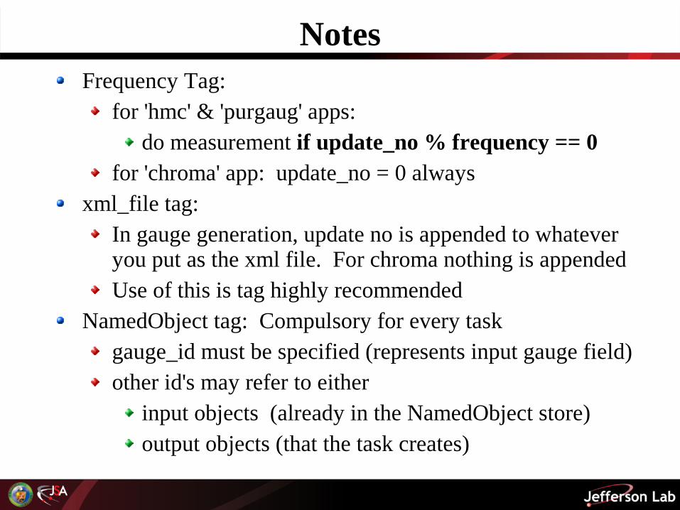
NotesFrequency Tag:
for 'hmc' & 'purgaug' apps:do measurement if update_no % frequency == 0
for 'chroma' app: update_no = 0 always xml_file tag:
In gauge generation, update no is appended to whatever you put as the xml file. For chroma nothing is appendedUse of this is tag highly recommended
NamedObject tag: Compulsory for every taskgauge_id must be specified (represents input gauge field)other id's may refer to either
input objects (already in the NamedObject store)output objects (that the task creates)

Some Useful XML GroupsThe following are groups found commonly in a lot of measurements. I will discuss the structure with examples.
<Cfg> read default configuration<RNG> seed random number generator<FermionAction> use fermion action
<anisoParam> -- parameters related to anisotropy<FermState> - To do with smearing, boundaries
<FermionBC><InvertParams> - to do with inverters

<Cfg>
<Cfg> <cfg_type>XXXXXX</cfg_type> <cfg_file>YYYYYY</cfg_file></Cfg>
Types of Files:SZIN, SZINQIO,
SCIDAC, NERSC, MILC, CPPACS, KYU
Types without Files:UNIT, DISORDERED,
WEAK_FIELD
This should be a filename for types with files. Ignored
for types withou files
" Gauge field here becomes: 'default_gauge_field'"SCIDAC reads ILDG as well

<RNG>
<RNG> <Seed> <elem>M0</elem> <elem>M1</elem> <elem>M2</elem> <elem>M3</elem> </Seed></RNG>
Sets up the random number Seed Random number generator is a linear congruential generator
with modulus m = 247
increment c = 0 multiplier a = 236 x M3 + 224x M2 + 212x M1 + M0

FermionAction
<FermionAction> <FermAct>XXXX</FermAct>
... <AnisoParam/> <FermState> <Name>YYYY</Name>
... <FermionBC> <FermBC>ZZZZ</FermBC> ... </FermionBC> </FermState>
</FermionAction>
Selects a Fermion Action, with Boundaries and Link States
Eg: WILSON, DWF etc
masses, etc
SIMPLE, Smearedetc
State params eg:n_smear
Name of boundary condition
Boundary related params

<AnisoParam>Controls Anisotropy Parameters:
<AnisoParam> <anisoP>false</anisoP> <t_dir>3</t_dir> <xi_0>1</xi_0> <nu>1</nu> </AnisoParam>
Are we really anisotropic?
'fine' direction
Bare gauge anisotropyFermion
Anisotropy
<AnisoParam> <anisoP>true</anisoP> <t_dir>3</t_dir> <xi_0>2.464</xi_0> <nu>0.95</nu> </AnisoParam>
Typical use for isotropic simulations:

FermionBC - Boundaries
<FermionBC> <FermBC>SIMPLE_FERMBC</FermBC> <boundary>1 1 1 -1</boundary></FermionBC>
<FermionBC> <FermBC>PERIODIC_FERMBC</FermBC></FermionBC>
1 = Periodic0 = Dirichlet
-1 = AntiperiodicBoundary Conditions in directions 0,1,2,3
respectively
Periodic in all directions

<FermState> - link states
<FermState> <Name>SIMPLE_FERM_STATE</Name> <FermionBC> ... </FermionBC></FermState>
<FermState> <Name>STOUT_FERM_STATE</Name> <rho>0.14</rho> <n_smear>2</n_smear> <orthog_dir>3</orthog_dir> <FermionBC> ... </FermionBC></FermState>
Thin Links- nothing special
Stout smearedlinks
2 hits withsmearing factor
0.14
Smear in directions orthogonal to this one
(set to 4 to smear all directions)

Wilson Fermion Action
<FermionAction> <FermAct>WILSON</FermAct> <Mass>-0.05</Mass> <AnisoParam/> <FermState/></FermionAction>
<FermionAction> <FermAct>WILSON</FermAct> <Kappa>0.123</Kappa> <AnisoParam/> <FermState/></FermionAction>
WILSON means 2 colour 4D- Schur Preconditioned Wilson.
use UNPRECONDITIONED_WILSONif you don't want the preconditioned op.

Clover Fermion Action
<FermionAction> <FermAct>CLOVER</FermAct> <Mass>-0.05</Mass> <clovCoeff>2.0171</clovCoeff> <AnisoParam/> <FermState/></FermionAction>
<FermionAction> <FermAct>CLOVER</FermAct> <Kappa>0.123</Kappa> <clovCoeffR>1.5</clovCoeffR> <clovCoeffT>0.9</clovCoeffT> <AnisoParam/> <FermState/></FermionAction>
CLOVER means 2 colour 4D- Schur Preconditioned CLOVER
use UNPRECONDITIONED_CLOVERif you don't want the preconditioned op.
Single coeff forisotropic case
Separate coeffs.for anisotropic case

DWF Fermion Action(s)<FermionAction> <FermAct>DWF</FermAct> <OverMass>1.2</OverMass> <Mass>0.4</Mass> <N5>4</N5> <AnisoParam/> <FermionBC/></FermionAction>
length of 5th dimension
4D Red-black preconditioned DWF
DWF Height
<FermionAction> <FermAct>NEF</FermAct> <OverMass>1.2</OverMass> <Mass>0.4</Mass> <N5>4</N5> <b5>1</b5> <c5>0</c5> <AnisoParam/> <FermionBC/></FermionAction>
Same but with4D preconditioned Moebius operator
Moebius may not support anisotropy :(

<InvertParam>
Controls the inverters:
<InvertParam> <invType>XXXXXXX</invType> ...</InvertParam>
Choose inverter
Inverter specificparameters
<InvertParam> <invType>CG_INVERTER</invType> <RsdCG>1.0e-8</RsdCG> <MaxCG>5000</MaxCG></InvertParam>
Typical usage:Conjugate Gradients
Target relativeresiduum
Maximum iterations

Multiple Shift SolversWhether a solver is a multiple shift solver or a single solution solver is 'determined from context'CG_SOLVER is a single solution solver in PROPAGATORbut may be a multi-shift solver in MULTI_PROPAGATOR
whether this is repeated single solves vs true multi shift solve is another question.
Multi-Shift systems can set individual residua for each shiftIf only one residuum is set � it is applied to each shiftShifts should be ordered (smallest leftmost, biggest rightmost)
<InvertParam> <invType>CG_INVERTER</invType> <RsdCG>1.0e-4 1.0e-6 1.0e-7</RsdCG> <MaxCG>5000</MaxCG></InvertParam>
RsdCG for smallest shift
RsdCG for largest shift

BiCGStab
<InvertParam> <invType>BICGSTAB_INVERTER</invType> <RsdBiCGStab>1.0e-8</RsdBiCGStab> <MaxBiCGStab>1000</MaxBiCGStab></InvertParam>
BiCGStab solver
Target residuum
Maximum Iters
BiCGStab solver is experimental. Seems ok for Wilson/Clover

Do a CG restart to 'polish' result
CG Solver allows a single restart Intended for mixed single/double prec solvers where
first solver is in single precision second solver is in double precision
Allows first solve to have single residuum... Designed specially for level 3 DWF solver needs configure flag � enable-cg-solver-restart
<InvertParam> <invType>CG_INVERTER</invType> <RsdCG>1.0e-8</RsdCG> <MaxCG>5000</MaxCG> <RsdCGRestart>1.0e-10</RsdCGRestart> <MaxCGRestart>1000</MaxCGRestart></InvertParam>
Target residuum for restart
MaxCG forrestart

Some Useful 'Measurements'Make Source / Propagator / Sink Smearing / Spectrum
Subject of tutorial exerciseI/O tasksNamed Object Management

Make Source
<elem> <Name>MAKE_SOURCE</Name> <Frequency>1</Frequency> <Param> <version>6</version> <Source> <version>2</version> <SourceType>SHELL_SOURCE</SourceType> <j_decay>3</j_decay> <t_srce>0 0 0 0</t_srce>
<SmearingParam/>
<Displacement/>
<LinkSmearing/> </Source> </Param>
<NamedObject> <gauge_id>default_gauge_field</gauge_id> <source_id>sh_source_1</source_id> </NamedObject> </elem> ID of created
source (output)
Can also be POINT_SOURCE . SHELL_SOURCE
means smeared quark source
time direction
Coordinates of centre of source
a.k.a. Fuzzing
quark field smearing details if source is SHELL_SOURCE
Point Split Operator details

More on MAKE_SOURCE
<SmearingParam> <wvf_kind>GAUGE_INV_GAUSSIAN</wvf_kind> <wvf_param>2.0</wvf_param> <wvfIntPar>5</wvfIntPar> <no_smear_dir>3</no_smear_dir></SmearingParam>
<Displacement> <version>1</version> <DisplacementType>NONE</DisplacementType></Displacement>
<LinkSmearing> <LinkSmearingType>APE_SMEAR</LinkSmearingType> <link_smear_fact>2.5</link_smear_fact> <link_smear_num>1</link_smear_num> <no_smear_dir>3</no_smear_dir></LinkSmearing>
Gauge Invariant quark source
smearing. 5 hits, rho=2.0, don't smear in direction 3 (time)
Group ignored for POINT_SOURCE
Not a displaced operator
1 hit of APE Fuzzing, with rho=2.1. Don't
smear in direction 3This group is optional. If not present, no fuzzing is done

FULL= relativistic 12 componensUPPER= nonrelativistic w.
LOWER=nonrelativistic w. (Nonrelativistic does 6 component
solves but still uses all 12 components of storage.)
PROPAGATOR
<elem> <Name>PROPAGATOR</Name> <Frequency>1</Frequency> <Param> <version>10</version> <quarkSpinType>FULL</quarkSpinType> <obsvP>false</obsvP> <FermionAction/> <InvertParam/> </Param> <NamedObject> <gauge_id>default_gauge_field</gauge_id> <source_id>sh_source_1</source_id> <prop_id>sh_prop_1</prop_id> </NamedObject> </elem>
Computes 12 Component 4D propagator
For 5D fermions (DWF) set to true to compute dim=5 axial currents
etc. This uses more memory tho as 12 Ls size vectors need to be stored
Output prop, created by task
Input source created byMAKE_SOURCE or
SEQSOURCE
Input gauge field

SINK_SMEAR <elem> <Name>SINK_SMEAR</Name> <Frequency>1</Frequency> <Param> <version>5</version> <Sink> <version>1</version> <SinkType>SHELL_SINK</SinkType> <j_decay>3</j_decay>
<SmearingParam/> <Displacement/> <LinkSmearing/>
</Sink> </Param> <NamedObject> <gauge_id>default_gauge_field</gauge_id> <prop_id>sh_prop_0</prop_id> <smeared_prop_id>sh_sh_prop_0</smeared_prop_id> </NamedObject> </elem>
Same as for MAKE_SOURCE
Same as for MAKE_SOURCE
Can be POINT_SINK
Input Prop
Output sink (smeared prop)

HADRON_SPECTRUM <elem> <Name>HADRON_SPECTRUM</Name> <Frequency>1</Frequency> <Param> <version>1</version> <MesonP>true</MesonP> <CurrentP>true</CurrentP> <BaryonP>true</BaryonP> <time_rev>false</time_rev> <mom2_max>3</mom2_max> <avg_equiv_mom>true</avg_equiv_mom> </Param> <NamedObject> <gauge_id>default_gauge_field</gauge_id> <sink_pairs> <elem> <first_id>sh_pt_sink_1</first_id> <second_id>sh_pt_sink_1</second_id> </elem> <elem> <first_id>sh_sh_sink_1</first_id> <second_id>sh_sh_sink_1</second_id> </elem> </sink_pairs> </NamedObject> <xml_file>hadspec.dat.xml</xml_file> </elem>
Which correlators to compute (mesons, currents, baryons) ?
Time reverse the baryons?
max
Average over correlators with
same
Dump to external file
Input sink quark propmade by
SINK_SMEAR
Input sink anti quark prop

Writing out Named Objects<elem> <Name>QIO_WRITE_NAMED_OBJECT</Name> <Frequency>1</Frequency> <NamedObject> <object_id>default_gauge_field</object_id> <object_type>Multi1dLatticeColorMatrix</object_type> </NamedObject> <File> <file_name>qio.cfg</file_name> <file_volfmt>MULTIFILE</file_volfmt> </File></elem>
ID of object to write
mirror QDP++ type name. Here use QDP++
native precision
<elem> <Name>QIO_WRITE_NAMED_OBJECT</Name> <Frequency>1</Frequency> <NamedObject> <object_id>default_gauge_field</object_id> <object_type>Multi1dLatticeColorMatrixD</object_type> </NamedObject> <File> <file_name>qio_double.cfg</file_name> <file_volfmt>SINGLEFILE</file_volfmt> </File></elem>
D = Double PrecisionF = Single Precision
fixed precision writes

Writing Propagators <elem> <Name>QIO_WRITE_NAMED_OBJECT</Name> <Frequency>1</Frequency> <NamedObject> <object_id>sh_prop_0</object_id> <object_type>LatticePropagator</object_type> </NamedObject> <File> <file_name>qio_propagator.lime</file_name> <file_volfmt>SINGLEFILE</file_volfmt> </File></elem>
This dumps the lattice propagator object to disk using QIONamed Object has associated � User Record XML� from the PROPAGATOR task.This predates � USQCD Standard� who use the record XML in other ways. We are working to resolve the differences.

Reading Named Objects<elem> <Name>QIO_READ_NAMED_OBJECT</Name> <Frequency>1</Frequency> <NamedObject> <object_id>redo_cfg</object_id> <object_type>Multi1dLatticeColorMatrix</object_type> </NamedObject> <File> <file_name>./qio.cfg</file_name> </File></elem>
File to read. QIO works out SINGLEFILE/MULTIFILE
automatically
This will be the ID of the Named Object
<elem> <Name>QIO_READ_NAMED_OBJECT</Name> <Frequency>1</Frequency> <NamedObject> <object_id>redo_prop</object_id> <object_type>LatticePropagator</object_type> </NamedObject> <File> <file_name>./qio_propagator.lime</file_name> </File></elem>
Propagators too
Should read ILDG as well

Legacy Formats: SZIN <elem> <Name>SZIN_WRITE_NAMED_OBJECT</Name> <Frequency>1</Frequency> <NamedObject> <object_id>default_gauge_field</object_id> <object_type>Multi1dLatticeColorMatrix</object_type> </NamedObject> <File> <file_name>szin.cfg</file_name> </File> </elem>
<elem> <Name>SZIN_READ_NAMED_OBJECT</Name> <Frequency>1</Frequency> <NamedObject> <object_id>redo_cfg</object_id> <object_type>Multi1dLatticeColorMatrix</object_type> </NamedObject> <File> <file_name>szin.cfg</file_name> </File> </elem>
No SINGLEFILE / MULTIFILE issue
Only gauge fields supported for SZIN a.t.m

Legacy Formats: NERSC
<elem> <Name>NERSC_WRITE_NAMED_OBJECT</Name> <Frequency>1</Frequency> <NamedObject> <object_id>default_gauge_field</object_id> </NamedObject> <File> <file_name>nersc.cfg</file_name> </File> </elem>
<elem> <Name>NERSC_READ_NAMED_OBJECT</Name> <Frequency>1</Frequency> <NamedObject> <object_id>foo</object_id> </NamedObject> <File> <file_name>nersc.cfg</file_name> </File> </elem>
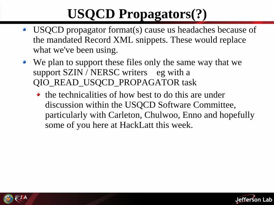
USQCD Propagators(?)USQCD propagator format(s) cause us headaches because of the mandated Record XML snippets. These would replace what we've been using.We plan to support these files only the same way that we support SZIN / NERSC writers � eg with a QIO_READ_USQCD_PROPAGATOR task
the technicalities of how best to do this are under discussion within the USQCD Software Committee, particularly with Carleton, Chulwoo, Enno and hopefully some of you here at HackLatt this week.
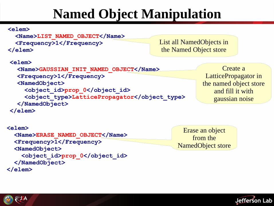
Named Object Manipulation<elem> <Name>LIST_NAMED_OBJECT</Name> <Frequency>1</Frequency></elem>
<elem> <Name>GAUSSIAN_INIT_NAMED_OBJECT</Name> <Frequency>1</Frequency> <NamedObject> <object_id>prop_0</object_id> <object_type>LatticePropagator</object_type> </NamedObject></elem>
<elem> <Name>ERASE_NAMED_OBJECT</Name> <Frequency>1</Frequency> <NamedObject> <object_id>prop_0</object_id> </NamedObject></elem>
List all NamedObjects in the Named Object store
Create a LatticePropagator in
the named object store and fill it with gaussian noise
Erase an object from the
NamedObject store

Named Object Manipulation<elem> <Name>QIO_WRITE_ERASE_NAMED_OBJECT</Name> <Frequency>1</Frequency> <NamedObject> <object_id>prop_0</object_id> <object_type>LatticePropagator</object_type> </NamedObject> <File> <file_name>./prop_0</file_name> <file_volfmt>MULTIFILE</file_volfmt> </File></elem>
Write object and then remove from
memory
Same info as for 'QIO_WRITE_NAMED_OBJECT'

HMC Basic Layout<?xml version=”1.0”?><Params> <MCControl> <Cfg> ... </Cfg> <RNG> ... </RNG>
<StartUpdateNum>0</StartUpdateNum> <NWarmUpUpdates>50</NWarmUpUpdates> <NProductionUpdates>20000</NProductionUpdates> <NUpdatesThisRun>10</NUpdatesThisRun> <SaveInterval>5</SaveInterval> <SavePrefix>./fred</SavePrefix> <SaveVolfmt>SINGLEFILE</SaveVolfmt> <ReproCheckP>true</ReproCheckP> <ReproCheckFrequency>10</ReproCheckFrequency>
<InlineMeasurements/> </MCControl>
I/O Related
Check reproducibility
Startup Config
Random Number Seed
Update Control

HMC Basic Layout II: </MCControl> <HMCTrj> <nrow>...</nrow>
<Monomials> <elem> .. </elem> </Monomials> <Hamiltonian> <monomial_ids>...</monomial_ids> </Hamiltonian>
<MDIntegrator> ... </MDIntegrator> </HMCTrj></Params>
Define List of Monomials here
each one has an ID
List IDs of monomials
that make up H here
Define the MD integrator
Lattice Size

Notes on the HMC Layout
<Cfg>, <RNG> <InlineMeasurements> - same as in chroma application modulo exceptions mentioned earlier<NProductionUpdates> refers to the whole ensemble. The number of trajectories to attempt is <NUpdatesThisRun><NWarmUpUpdates> - turns off the Accept/Reject test and always accepts. Useful for cold/hot starts where initial energy changes can be HUGE.If <ReproCheckP> is ommitted the default is that it is enabled at 10% (Ie every 10 iterations)In <Monomials> we define monomials as NamedObject
refer to them by name in Hamiltonian/Integrator.
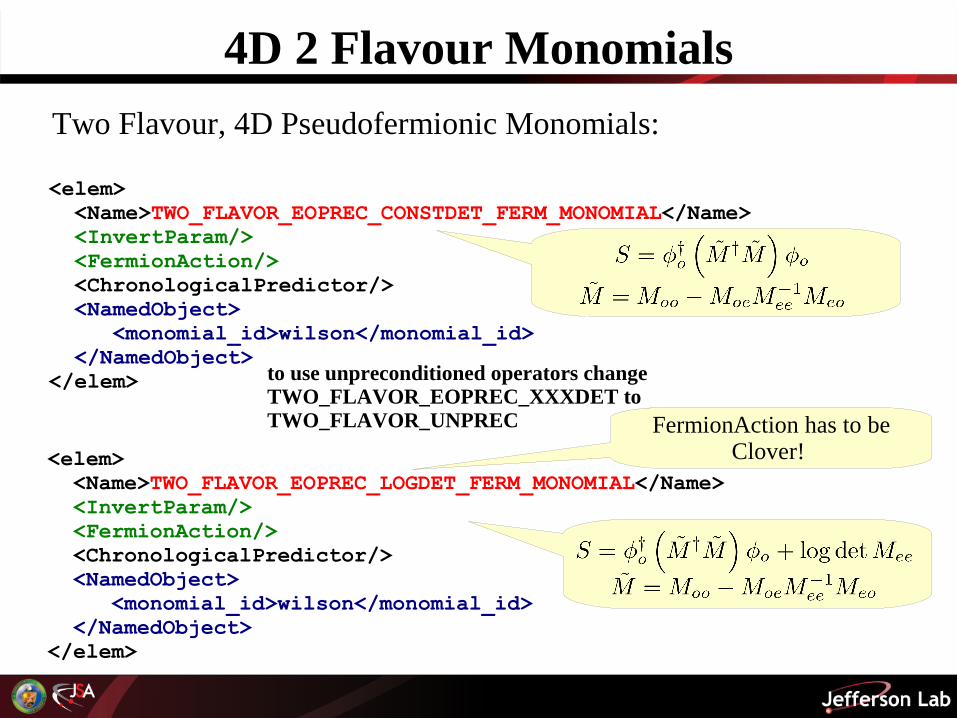
4D 2 Flavour Monomials
<elem> <Name>TWO_FLAVOR_EOPREC_CONSTDET_FERM_MONOMIAL</Name> <InvertParam/> <FermionAction/> <ChronologicalPredictor/> <NamedObject> <monomial_id>wilson</monomial_id> </NamedObject></elem>
Two Flavour, 4D Pseudofermionic Monomials:
<elem> <Name>TWO_FLAVOR_EOPREC_LOGDET_FERM_MONOMIAL</Name> <InvertParam/> <FermionAction/> <ChronologicalPredictor/> <NamedObject> <monomial_id>wilson</monomial_id> </NamedObject></elem>
FermionAction has to be Clover!
to use unpreconditioned operators change TWO_FLAVOR_EOPREC_XXXDET toTWO_FLAVOR_UNPREC
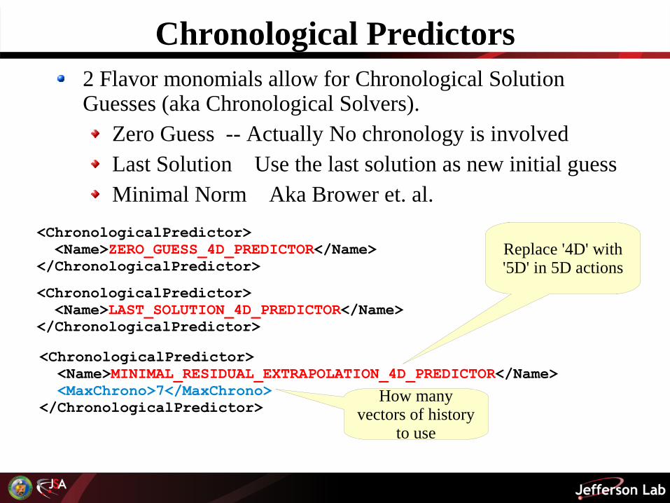
Chronological Predictors2 Flavor monomials allow for Chronological Solution Guesses (aka Chronological Solvers).
Zero Guess -- Actually No chronology is involvedLast Solution � Use the last solution as new initial guessMinimal Norm � Aka Brower et. al.
<ChronologicalPredictor> <Name>LAST_SOLUTION_4D_PREDICTOR</Name></ChronologicalPredictor>
<ChronologicalPredictor> <Name>ZERO_GUESS_4D_PREDICTOR</Name></ChronologicalPredictor>
<ChronologicalPredictor> <Name>MINIMAL_RESIDUAL_EXTRAPOLATION_4D_PREDICTOR</Name> <MaxChrono>7</MaxChrono></ChronologicalPredictor>
How many vectors of history
to use
Replace '4D' with '5D' in 5D actions

Just The Even-Even Clover Bit
<elem> <Name>N_FLAVOR_LOGDET_EVEN_EVEN_FERM_MONOMIAL</Name> <FermionAction/> <num_flavors>2</num_flavors> <NamedObject> <monomial_id>logdet_clover_2flav_ee</monomial_id> </NamedObject></elem>

Rational Single Flavour
<elem> <Name>ONE_FLAVOR_EOPREC_CONSTDET_FERM_RAT_MONOMIAL</Name> <expNumPower>1</expNumPower> <expDenPower>1</expDenPower> <nthRoot>1</nthRoot> <InvertParam/> <FermionAction/> <Remez> <lowerMin>8</lowerMin> <upperMax>40</upperMax> <forceDegree>10</forceDegree> <actionDegree>14</actionDegree> </Remez> <NamedObject> <monomial_id>fermion</monomial_id> </NamedObject></elem>
ab
rational approx for
Approximation bounds Approximation degree (number of poles after partial fraction expansion)
to use unpreconditioned operators change EOPREC_CONSTDET to UNPREC
deals with:

Hasenbusch
<elem> <Name>TWO_FLAVOR_EOPREC_CONSTDET_HASENBUSCH_FERM_MONOMIAL</Name> <InvertParam/> <FermionAction> <FermionActionPrec/> <ChronologicalPredictor/> <NamedObject> <monomial_id>hasenbusch</monomial_id> </NamedObject></elem>
Gives M at desired parameters
Gives M2 at heavier mass/other params
evaluates:
Note, the preconditioner needs to still be cancelled off with a second, normal 2 Flavour monomialchange EOPREC_CONSTDET to UNPREC for unpreconditioned
fermions matrices.

2 Flavor 5D Actions<elem> <Name>TWO_FLAVOR_EOPREC_CONSTDET_FERM_MONOMIAL5D</Name> <InvertParam/> <FermionAction/> <ChronologicalPredictor/> <NamedObject> <monomial_id>dwf</monomial_id> </NamedObject></elem>
Difference in 'name only' just slap '5D' on there.
This needs to be a 5D
action now
As usual change EOPREC_CONSTDET to UNPREC for unpreconditioned operatorsHASENBUSCH very similar
TWO_FLAVOR_EOPREC_CONSTDET_HASENBUSCH_FERM_MONOMIAL5D
<FermionActionPrec> needs to be added
MPV
gets swapped to M2 in the formula above (PV operators cancel)

1 Flavor 5D Actions<elem> <Name>ONE_FLAVOR_EOPREC_CONSTDET_FERM_RAT_MONOMIAL5D</Name> <nthRoot>1</nthRoot> <nthRootPV>1</nthRootPV> <expNumPower>1</expNumPower> <expDenPower>1</expDenPower> <FermionAction/> <InvertParam/>
<Remez> <lowerMin>0.001</lowerMin> <upperMax>5.8</upperMax> <lowerMinPV>0.001</lowerMinPV> <upperMaxPV>5.8</upperMaxPV> <degree>10</degree> <degreePV>10</degreePV> </Remez> <NamedObject> <monomial_id>dwf_1flav</monomial_id> </NamedObject></elem>
Separate bounds for Pauli Villars operator
Separate approximation degree
for PV
Separate n-th rootery option for PV
NB: No forceDegree/actionDegree option here. Make separate
objects for MD, H

Gauge Action Monomials
<elem> <Name>GAUGE_MONOMIAL</Name> <GaugeAction> <Name>WILSON_GAUGEACT</Name> ... <GaugeState> <Name>SIMPLE_GAUGE_STATE</Name> ... <GaugeBC> <Name>PERIODIC_GAUGEBC</Name> ... </GaugeBC> </GaugeState> </GaugeAction> <NamedObject> <monomial_id>gauge</monomial_id> </NamedObject></elem>
<GaugeAction> mirrors the <FermionAction> structure with a <GaugeState> and a <GaugeBC>Both the <GaugeAction>, <GaugeState> and <GaugeBC> may have their own parameters (...)Most conventional simulations will use SIMPLE_GAUGE_STATE and PERIODIC_GAUGEBC
these have no extra params

Wilson Gauge Monomial <elem> <Name>GAUGE_MONOMIAL</Name> <GaugeAction> <Name>WILSON_GAUGEACT</Name> <beta>5.2</beta>
<AnisoParam> <anisoP>true</anisoP> <t_dir>3</t_dir> <xi_0>2.464</xi_0> </AnisoParam> <GaugeState> <Name>SIMPLE_GAUGE_STATE</Name> <GaugeBC> <Name>PERIODIC_GAUGEBC</Name> </GaugeBC> </GaugeState>
</GaugeAction> <NamedObject> <monomial_id>gauge</monomial_id> </NamedObject> </elem>
Beta is the only coupling here
Gauge Anisotropy parameters. Identical to
Fermion except there is no 'nu' parameter
This is most typical. Older versions (before GaugeState)
may just have the <GaugeBC> tag without the <GaugeState> surrounding
it . That works for backward compatibility for now.

Improved Gauge ActionsWe have separate Plaquette and Rectangle terms that can be used 'Raw':
<elem> <Name>GAUGE_MONOMIAL</Name> <GaugeAction> <Name>RECT_GAUGEACT</Name> <coeff>-0.46296296296296296296</coeff> <AnisoParam> <anisoP>false</anisoP> <t_dir>3</t_dir> <xi_0>1</xi_0> </AnisoParam> <GaugeState/> </GaugeAction>
<NamedObject> <monomial_id>gauge</monomial_id> </NamedObject> </elem>
coefficient of rectangle terms

Improved Gauge Actions Various wrappers combine Plaq + Rectangle terms: eg: Tree level LW. or RG improved etc...
<elem> <Name>GAUGE_MONOMIAL</Name> <GaugeAction> <Name>LW_TREE_GAUGEACT</Name> <beta>7.5</beta> <u0>0.9</u0> <AnisoParam/> <GaugeState/> </GaugeAction> <NamedObject/></elem>
<elem> <Name>GAUGE_MONOMIAL</Name> <GaugeAction> <Name>RG_GAUGEACT</Name> <beta>1.8</beta> <c1>0.6</c1> <AnisoParam/> <GaugeState/> </GaugeAction> <NamedObject/></elem>
Work c0, c1 etc from u0
RG conventions: c0 from beta and
normalization(?)

Hamiltonian
<Hamiltonian> <monomial_ids> <elem>rat1</elem> <elem>rat2</elem> <elem>rat3</elem> <elem>gauge</elem> </monomial_ids></Hamiltonian>
This is really simple it is just a list of monomial-ids that are needed in the Hamiltonian. Below is an example with 4 monomials (momenta are implied). Potentially 3 single flavor rational monomials + 1 gauge piece
These monomials have to have been declared in the <Monomials> section

MD Integrator
<MDIntegrator> <tau0>1.0</tau0> <copyList> <elem> <copyFrom>rat1_mc</copyFrom> <copyTo>rat1_md</copyTo> </elem> ... </copyList>
<anisoP>true</anisoP> <t_dir>3</t_dir> <xi_mom>3.5</xi_mom>
<Integrator> ... </Integrator></MDIntegrator>
The description of the integrator scheme
Trajectory Length
It can happen that the same term in the action is represented by a different monomial in the 'Energy'
calculation and in the MD. (eg MD has slightly different parameters than
the monomial for the energy for algorithmic
reasons)
In that case the dynamical fields of the
'Energy' monomials, need to be copied into the MD
monomials.
If the MC and MD monomials are the same,
the copy list can be omitted.
monomial_id of monomial to copy to
monomial_id of monomial to copy from
Anisotropic integration.The momenta in t_dir are
rescaled by a factor of 1/xi_mom (shorter steps)
--this is optional
The actual choice of integrators, timesteps etc....

Integrator � general scheme<Integrator> <Name>XXXX</Name> <n_steps>15</n_steps> <monomial_ids> <elem>rat1_md</elem> ... </monomial_ids> .... <SubIntegrator> <Name>YYYY</Name> <n_steps>3</n_steps> <monomial_ids> <elem>gauge</elem> </monomial_ids> .... </SubIntegrator> </Integrator>
Name of integrator component
No of steps w.r.t tau0 (outermost integrator)
Array of monomials to integrate on this timescale
Other parameters, eg tuning constants for Omelyan integrators
Optional sub integrator(which may have optional sub
integrators etc)
These n_steps are with respect to the timescale of the parent integrator. So in this
case 1/15*1/3 = 1/45 wrt tau0

Leapfrog Integrator
<Integrator> <Name>LCM_STS_LEAPFROG</Name> <n_steps>10</n_steps> <monomial_ids><elem>gauge</elem></monomial_ids></Integrator>
STS means update with S (potential energy piece), then T (kinetic energy piece) then S again. Update with S updates the momenta, so this would also be known as a PQP integratorTST variant (QPQ) also available: LCM_TST_LEAPFROG
NB: No SubIntegrator in this example, but you could put one in.here if you wanted

2nd Order Omelyan
TST variant is also availableIf lambda is not given, the value from the deForcrand � Takaishi paper is used.
<Integrator> <Name>LCM_STS_MIN_NORM_2</Name> <n_steps>5</n_steps> <monomial_ids><elem>ferm_2flav_hasen</elem></monomial_ids> <lambda>0.19</lambda>
<SubIntegrator> <Name>LCM_STS_MIN_NORM_2</Name> <n_steps>2</n_steps> <monomial_ids><elem>ferm_2flav_cancel</elem></monomial_ids> <lambda>0.19</lambda> </SubIntegrator></Integrator>
Name for Omelyan: MIN_NORM_2
Tunable parameter for Omelyan
In this example I have a 2nd timescale, but this is
'optional'

4th Order<Integrator> <Name>LCM_CREUTZ_GOCKSCH_4</Name> <n_steps>10</n_steps> <monomial_ids><elem>gauge</elem></monomial_ids></Integrator>
<Integrator> <Name>LCM_4MN4FP</Name> <n_steps>10</n_steps> <rho>0.1786178958448091</rho> <theta>-0.06626458266981843</theta> <lambda>0.7123418310626056</lambda> <monomial_ids><elem>gauge</elem></monomial_ids></Integrator>
<Integrator> <Name>LCM_4MN5FP</Name> <n_steps>10</n_steps> <rho>0.2539785108410595</rho> <theta>0.08398315262876693</theta> <lambda>0.6822365335719091</lambda> <mu>-0.03230286765269967</mu> <monomial_ids><elem>gauge</elem></monomial_ids></Integrator>
Basic Creutz/Gocksch Campostrini, scheme
4th order Omelyan (minimum norm) (4MN)
4 forces per step (4F)'position' variant (P)
tunable parameters defaults values are from deForcrand & Takaishi paper
4th order Omelyan (4MN)5 forces per step (5F)'position' variant (P)
'velocity' variant is also available: 4MN5FV

A note on the 4th order integratorsNaturally the 4th order integrators also support sub-integrators etc
I have found that 4th order integrators NEED double precision. In single precision, the error stopped decreasing for step sizes below ~ 0.1-0.01 � so beware when using these. They seemed to work (reproduce graphs from deForcrand & Takaishi) when using double precision.

That wasn't so bad was it?the XML has structure binds tightly to the underlying class structures...