GSTARS4 User's Manual
124
User’s Manual for GSTARS4 (Generalized Sediment Transport model for Alluvial River Simulation version 4.0) by Chih Ted Yang and Jungkyu Ahn 2011 Hydroscience and Training Center Colorado State University
Transcript of GSTARS4 User's Manual

User’s Manual for
GSTARS4
(Generalized Sediment Transport model for Alluvial River Simulation
version 4.0)
by
Chih Ted Yang
and
Jungkyu Ahn
2011
Hydroscience and Training Center
Colorado State University

Hydroscience and Training Center
Colorado State University
Acknowledgement
The authors appreciate the financial supports provided by the Omaha District, US Army
Corps of Engineers for the development, testing, and application of the GSTARS4
computer program.
i
TABLE OF CONTENTS
1. Introduction …………………………………………………………………….… 1 1.1 Purpose and Capabilities …………………………………………………………… 1
1.1.1 What is New in GSTARS4 ……………………………………………...……… 4
1.2 Limits of Application ………………………………………………………….…… 4
1.3 Overview of the Manual …………………………………………………………… 5
1.4 Acquiring GSTARS4 ………………………………………………………………. 5
1.5 Disclaimer ……………………………………………………………………..…… 5
2. The Hydraulic Computation ……………………………………………..…… 7 2.1 Steady Flow Computation ………………………………………………………….. 8
2.1.1 Energy Equation ………………………………………………………………… 8
2.1.2 Flow Transitions ………………………………………………………………... 9
2.1.3 Normal, Critical, and Sequent Depth Computations …………………………. 10
2.1.4 Model Representation …………………………………………………………. 11
2.1.5 Tributary Influence ……………………………………………………………. 18
2.1.5.1 Table Form of Inflow from Tributaries ……………………………………. 18
2.1.5.2 Interchanges between a Tributary and the Main Stream …………………... 18
2.2 Unsteady Flow Computation ……………………………………………………… 20
2.2.1 Governing Equations ………………………………………………………….. 20
2.2.2 Numerical Scheme …………………………………………………………….. 21
3. Sediment Routing and Channel Geometry Adjustment …………….... 24 3.1 Governing Equations ……………………………………………………………... 25
3.1.1 Theoretical Background ……………………………………………………….. 25
3.1.2 Sediment Continuity Equation ………………………………………………… 25
3.2 Streamlines and Stream Tubes ……………………………………………………. 26
3.3 Discretization of the Governing Equations ……………………………………….. 29
3.3.1 Transmissive Cross Sections …………………………………………………... 31
3.3.2 Numerical Stability ……………………………………………………………. 32
3.3.3 Additional Comments …………………………………………………………. 32
3.4 Bed Sorting and Armoring ………………………………………………………... 33
3.4.1 Remarks ……………………………………………………………………….. 37
3.5 Sediment Transport Functions ……………………………………………………. 37
3.5.1 DuBoys’ Method (1879) ………………………………………………………. 39
3.5.2 Meyer-Peter and Muller's Formula (1948) ……………………………………. 40
3.5.3 Laursen's Formula (1958) and Modification by Madden(1993) ………………. 40
3.5.4 Toffaleti's Method (1969) ……………………………………………………... 41
3.5.5 Engelund and Hansen's Method (1972) ……………………………………….. 41
3.5.6 Ackers and White's Method (1973) and (1990) ……………………………….. 42
3.5.7 Yang's Sand (1973) and Gravel (1984) Transport Formulae ………………….. 43
3.5.8 Yang's Sand (1979) and Gravel (1984) Transport Formulae ………………….. 44
3.5.9 Parker's Method (1990) ………………………………………………………... 45

ii
3.5.10 Yang's Modified Formula for Sand Transport with High Concentration of Wash
Load (1996) …………………………………………………………………... 46
3.5.11 Tsinghua University Equation for Reservoir Flushing ………………………. 46
3.5.12 Ashida and Michiue Method (1972) …………………………………………. 47
3.6 Cohesive Sediment Transport …………………………………………………….. 49
3.6.1 Deposition …………………………………………………………………...… 51
3.6.2 Erosion ………………………………………………………………………… 53
3.7 Non-equilibrium Sediment Transport …………………………………………….. 55
3.8 Particle Fall Velocity Calculations ……………………………………………….. 58
4. Computation of Width Changes ……………………………………………. 61 4.1 Theoretical Basis ………………………………………………………………….. 61
4.2 Computational Procedures ………………………………………………………... 62
4.3 Channel Side Slope Adjustments …………………………………………………. 64
5. Reservoir Routing ……………………………………………………………… 66 5.1 Reservoir Routing ………………………………………………………………… 66
5.2 Sediment Transport ……………………………………………………………….. 70
6. Data Requirements …………………………………………………………….. 72 6.1 Input Data Format ………………………………………………………………… 72
6.2 Hydraulic Data ……………………………………………………………………. 73
6.2.1 Channel Geometry, Roughness, and Loss Coefficient Data …………………... 73
6.2.2 Discharge and Stage Data for Quasi-steady Flow Simulation ………………… 77
6.2.2.1 Discharge Hydrograph with a Stage-Discharge Rating Curve …………….. 78
6.2.2.2 Table of Discharges with a Rating Curve at The Control Section …………. 80
6.2.2.3 Stage-Discharge Table at a Control Section ……………………………….. 81
6.2.2.4 Reservoir Routing with Table of Discharges ………………………………. 82
6.2.2.5 Reservoir Routing with Discretized Discharges …………………………… 83
6.2.3 Discharge and Stage Data for Truly Unsteady Flow Simulation ……………… 84
6.2.3.1 Upstream Flow Boundary Condition ………………………………………. 84
6.2.3.2 Downstream Flow Boundary Condition …………………………………… 85
6.3 Sediment Data …………………………………………………………………….. 88
6.3.1 Sediment Inflow Data …………………………………………………………. 91
6.3.2 Temperature Data ……………………………………………………………… 95
6.3.3 Sediment Gradation Data ……………………………………………………… 95
6.3.3.1 Remarks …………………………………………………………………... 101
6.3.4 Cohesive Sediment Transport Parameters …………………………………… 105
6.3.5 Transfer of Sediment Across Stream Tube Boundaries ……………………… 106
6.3.6 Erosion and Deposition Limits ………………………………………………. 107
6.4 Output Control …………………………………………………………………... 108
6.5 Stream Power Minimization Procedure Data …………………………………… 109
6.6 Tributary Inflow/Outflow Data ………………………………………………….. 110
6.6.1 Table Form of Inflows from Tributaries ……………………………………... 110
6.6.2 Interchanges between a Tributary and the Main Stream …………………….. 112
6.7 Using GSTARS4 in Command Line Mode ……………………………………... 112
iii
6.8 Compatibility with Earlier Versions …………………………………………….. 114
References ……………………………………………………………………………. 115
Appendix A
List of input data records used in GSTARS4
Appendix B
Example application of GSTARS4
Example 1: Water Surface Calculation
Exmaple 2: Main Channel With One Tributary Inflow
Example 3: Sediment Transport in A Curved Channel
Example 4: Lake Mescaleroo Spillway Channel
Example 5: Reservoir Routing and Volume Computations
Example 6: Rio Grande Floodway
Example 7: Tarbela Reservoir, Pakistan
Example 8: Simulation of Channel Migration in the All American Canal
Example 9: Sedimentation and Flushing in the Xiaolangdi Reservoir
Example 10: Long Term Sedimentation in the Lewis and Clark Reservoir
Example 11: Flushing in Lewis and Clark Reservoir
Appendix C
Generalized water surface profile computation
Appendix D
Applicability of sediment transport formulas
1
CHAPTER
1
INTRODUCTION
GSTARS4 (Generalized Sediment Transport model for Alluvial River Simulation version
4.0) is the most recent version of a series of numerical models for simulating the flow of
water and sediment transport in alluvial rivers developed at the Hydroscience and
Training Center of Colorado State University. It is an enhanced version of the GSTARS3
model (Yang and Simões, 2002). This manual describes the overall theoretical
background of the model and its most important implementation details in a computer
program. It also guides the interested user in all the steps necessary for data preparation
and input. Examples of the application of GSTARS4 are also given.
1.1 Purpose and Capabilities
The GSTARS series of programs were developed due to the need for a generalized water
and sediment-routing computer model that could be used to solve complex river

2
engineering problems for which limited data and resources were available. In order to be
successful, such a model should have a number of capabilities, namely:
• It should be able to compute hydraulic parameters for open channels with fixed as well
as with movable boundaries;
• It should have the capacity of computing water surface profiles in the subcritical,
supercritical, and mixed flow regimes, i.e., in combinations of subcritical and
supercritical flows without interruption;
• It should have the capability of computing both steady and truly unsteady flow;
• It should be able to simulate and predict the hydraulic and sediment variations both in
the longitudinal and in the transverse directions;
• It should be able to simulate and predict the change of alluvial channel profile and
cross-sectional geometry, regardless of whether the channel width is variable or fixed;
and
• It should incorporate site specific conditions such as channel side stability and erosion
limits.
GSTARS version 4.0 is based on GSTARS version 3.0 (Yang and Simões, 2002) and
SRH-1D (Sediment and River Hydraulics –One dimension) (Huang and Greimann, 2007).
GSTARS4 adopted unsteady flow computational scheme and method from SRH-1D with
some revisions. For other capabilities, such as steady/quasi-steady flow computation
sediment calculation, and channel geomorphic changes, GSTARS4 uses almost the same
method that used for GSTARS3 with some modifications.
GSTARS4 consists of four major parts.
The first part is the use of both the energy and the momentum equations for the
backwater computations. This feature allows the program to compute the water surface
profiles through combinations of subcritical and supercritical flows. In these
computations, GSTARS4 can handle irregular cross sections regardless of whether single
channel or multiple channels separated by small islands or sand bars. The major update
was made for hydraulic calculation. Previous GSTARS models, GSTARSRS 1.0, 2.0, 2.1,
and 3.0, have the capability of steady or quasi-steady hydraulic computation whereas
GSTARS4 can simulate both steady and truly unsteady flow. The numerical scheme used
for unsteady computation was adopted from GSTAR-1D 1.0 (Yang, et al 2004) and SRH-
1D (Hung and Greimann, 2007) unsteady flow modules. SRH-1D is an improved and
enhanced model of GSTAR-1D 1.0 supported by the U.S. Bureau of Reclamation.
Unsteady flow computations in GSTARS4 are based on SRH-1D.
The second part is the use of the stream tube concept, which is used in the sediment
routing computations. Hydraulic parameters and sediment routing are computed for each
stream tube, thereby providing a transverse variation in the cross section in a semi-two-
dimensional manner. Although no flow can be transported across the boundary of a
stream tube, transverse bed slope and secondary flows are phenomena accounted for in
GSTARS4 that contribute to the exchange of sediments between stream tubes. The
position and width of each stream tube may change after each step of computation. The
scour or deposition computed in each stream tube give the variation of channel geometry
3
in the vertical (or lateral) direction. The water surface profiles are computed first. The
channel is then divided into a selected number of stream tubes with the following
characteristics: (1) the total discharge carried by the channel is distributed equally among
the stream tubes; (2) stream tubes are bounded by channel boundaries and by imaginary
vertical walls; (3) the discharge along a stream tube is constant (i.e., there is no exchange
of water through stream tube boundaries).
Bed sorting and armoring in each stream tube follows the method proposed by Bennett
and Nordin (1977), and the rate of sediment transport can be computed using any of the
following methods:
• DuBoys’ 1879 method
• Meyer-Peter and Muller's 1948 method.
• Laursen's 1958 method.
• Modified Laursen’s method by Madden (1993)
• Toffaleti's 1969 method.
• Engelund and Hansen's 1972 method.
• Ackers and White's 1973 method.
• Revised Ackers and White's 1990 method.
• Yang's 1973 sand and 1984 gravel transport methods.
• Yang's 1979 sand and 1984 gravel transport methods.
• Parker's 1990 method.
• Yang's 1996 modified method for high concentration of wash load.
• Ashida and Michiue’s 1972 method.
• Tsinghua University method (IRTCES, 1985).
• Krone's 1962 and Ariathurai and Krone's 1976 methods for cohesive sediment transport.
GSTARS4 uses the same numerical scheme as that in GSTARS3 for sediment routing
part with some minor revisions.
The third part is the use of the theory of minimum energy dissipation rate (Yang, 1971,
1976; Yang and Song, 1979, 1986) in its simplified version of minimum total stream
power to compute channel width and depth adjustments. The use of this theory allows the
channel width to be treated as an unknown variable. Treating the channel width as an
unknown variable is one of the most important capabilities of GSTARS4. Whether a
channel width or depth is adjusted at a given cross section and at a given time step
depends on which condition results in less total stream power. For the use of theory of
minimum energy dissipation rate, GSTARS4 is the same as the previous GSTARS3
model.
The fourth part is the inclusion of a channel bank side stability criteria based on the angle
of repose of bank materials and sediment continuity. GSTARS3 and GSTARS4 use
identical procedure for the calculation of bank side stability.
Some of the potential applications and/or features of GSTARS4 are:
• GSTARS4 can be used for water surface profile computations with or without sediment
transport by using steady and unsteady scheme.

4
• GSTARS4 can compute water surface profiles through subcritical and supercritical flow
conditions, including hydraulic jumps, without interruption.
• GSTARS4 can compute the longitudinal and transversal variations of flow and
sediment conditions in a semi-two-dimensional manner based on the stream tube concept.
If only one stream tube is selected, the model becomes one-dimensional. If multiple
stream tubes are selected, both the lateral and vertical bed elevation changes can be
simulated.
• The bed sorting and armoring algorithm is based on sediment size fractions and can
provide a realistic simulation of the bed armoring process.
• GSTARS4 can simulate channel geometry changes in width and depth simultaneously
based on minimum total stream power.
• The channel side stability option allows simulation of channel geometry change based
on the angle of repose of bank materials and sediment continuity.
1.1.1 What is New in GSTARS4
GSTARS4 is based on GSTARS3 with the following modifications and improvements:
• Unsteady flow simulation was added.
• More options for non-equilibrium sediment transport were added.
• Input option of percentage of washload were expanded in case of high sediment
concentration laden flows.
• Spatial variation of bed material density can be applicable.
• More options for gradation of incoming sediment from the upstream boundary.
• Water and sediment exchanges between the main channel and tributaries were added.
• Another output file for water and sediment discharges at the downstream boundary is
added for other uses, such as downstream impact routing.
• Expanded user’s manual
Although most data files prepared for GSTARS3 are fully compatible with GSTARS4,
only a few exceptions exist. Therefore, conversion of data files from GSTARS3 to
GSTARS4 is easy and straightforward.
1.2 Limits of Application
GSTARS4 is a general numerical model developed for a personal computer to simulate
and predict river and reservoir morphological changes caused by natural and engineering
events. Although GSTARS4 is intended to be used as a general engineering tool for
solving fluvial hydraulic problems, it does have the following limitations from a
theoretical point of view:
1. GSTARS4 is a semi-two-dimensional model for flow simulation and a semi-three-
dimensional model for simulation of channel geometry change. It should not be applied
to situations where a truly two-dimensional or truly three-dimensional model is needed
for detailed simulation of local conditions. However, GSTARS4 should be adequate for
solving many river engineering problems.
5
2. GSTARS4 is based on the stream tube concept. Secondary currents are empirically
accounted for. The phenomena of diffusion, and super elevation are ignored.
3. Many of the methods and concepts used in GSTARS4 are simplified approximations of
real phenomena. Those approximations and their limits of validity are, therefore,
embedded in the model.
1.3 Overview of the Manual
This manual is organized into six chapters (including this one) and four appendices.
Most parts of the GSTARS4 User’s Manual are identical to those in GSTARS3 because
the former is based on the latter except reservoir routing and tributary routing were
improved and enhanced..
Chapter 2 describes the hydraulic calculations with additional explanations on unsteady
flow scheme, and chapter 3 describes the basis of the sediment routing model, including
the use of the stream tube concept with some more explanations of new capability of
GSTARS4 model. Chapter 4 presents the concepts and the methodology used in the
channel width adjustment model. Chapter 5 presents the concepts used for water and
sediment routing in reservoirs. Chapter 4 and chapter 5 are the same as those of
GSTARS3. Finally, the main data requirements for GSTARS4 are discussed in chapter 6
with some additions for the new capability. The appendices provide additional
information: appendix A gives a detailed description of the input records used by
GSTARS4 and new capability are clear stated; appendix B provides several examples to
show some of the model's features and to help the user get started; appendix C contains a
reprint of the paper by Molinas and Yang (1985) that describes with more detail the basis
of the backwater algorithm used in GSTARS3 and GSTARS4; and appendix D contains a
reprint of the paper by Yang and Huang (2000) that offers guidelines on how to use
selected sediment transport capacity equations.
1.4 Acquiring GSTARS4
The latest information about the GSTARS4 program is placed on the World Wide Web.
The deleat the unnecessary space between words GSTARS4 Web page can be found by
going to www.engr.colostate.edu/ce/facultystaff/yang and following the links therein.
All questions regarding GSTARS4 should be sent to the first author. Dr. Chih Ted Yang
is the Director of Hydroscience and Training Center at Colorado State University, Fort
Collins, CO 80523 ([email protected]). Request can also be sent to the first
author directly ([email protected]).
GSTARS4 is in a stage of continuous evolution and unannounced changes may be made
at any time. The user is encouraged to check regularly the GSTARS4 Web page. Updates
to the code and documentation will be posted there as they become available.
1.5 Disclaimer
The program and information contained in this manual are developed by the
Hydroscience and Training Center (HTC) at Colorado State University. HTC does not
guarantee the performance of the program, nor help external users solve their problems.

6
HTC assumes no responsibility for the correct use of GSTARS4 and makes no warranties
concerning the accuracy, completeness, reliability, usability, or suitability for any
particular purpose of the software or the information contained in this manual. GSTARS4
is a complex program that requires engineering expertise to be used correctly. Like any
computer program, GSTARS4 cannot be certified infallible. All results obtained from the
use of the program should be carefully examined by an experienced engineer to
determine if they are reasonable and accurate. HTC and the GSTARS4 manual authors
will not be liable for any special, collateral, incidental, or consequential damages in
connection with the use of the software.
7
CHAPTER
2
THE HYDRAULIC COMPUTATION
The hydraulic computations in GSTARS4 are based on a model of gradually varied flow.
Mixed flow regimes and hydraulic jumps can be calculated by selectively using the
energy and the momentum equations. GSTARS4 model has capability of both steady and
unsteady flow simulations. This section presents the basic governing equations for flow
computations.
Steady or quasi steady computation in GSTARS4 model is the same as that of GSTARS3.
The basic concepts and backwater computational procedures can be found in most open
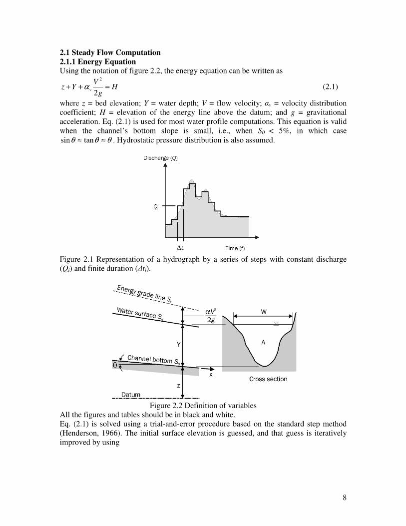
channel hydraulics text books. For quasi-steady flows, discharge hydrographs are
approximated by bursts of constant discharge, as shown in figure 2.1. During each
constant discharge burst, steady state equations are used for the backwater computations.
GSTARS3 and GSTARS4 solve the energy equation based on the standard-step method.
However, when a hydraulic jump occurs, the momentum equation is used instead. Details
of these computations were presented by Molinas and Yang (1985) and are given in
appendix C. Reservoir routing uses a modified standard step method and level-pool flood
routing. Governing equations and numerical schemes for steady or quasi-steady
simulations are explained in section 2.1. Section 2.1.4 (b) provides additional
explanations of GSTARS4 capacities. The explanations are similar to those shown in the
GSTARS3 User’s Manual.
For unsteady hydraulic routing, GSTARS4 model uses unsteady computation scheme of
SRH-1D with some revisions. Section 2.2 includes explanations on the unsteady flow
solutions and most explanations on unsteady flow solution in this section can also be
found in SHR-1D (Huang and Greimann,2007).
8
2.1 Steady Flow Computation
2.1.1 Energy Equation Using the notation of figure 2.2, the energy equation can be written as
Hg
VYz v =++
2
2
α (2.1)
where z = bed elevation; Y = water depth; V = flow velocity; αv = velocity distribution
coefficient; H = elevation of the energy line above the datum; and g = gravitational
acceleration. Eq. (2.1) is used for most water profile computations. This equation is valid
when the channel’s bottom slope is small, i.e., when S0 < 5%, in which case
θθθ ≈≈ tansin . Hydrostatic pressure distribution is also assumed.
Figure 2.1 Representation of a hydrograph by a series of steps with constant discharge
(Qi) and finite duration (∆ti).
Figure 2.2 Definition of variables
All the figures and tables should be in black and white.
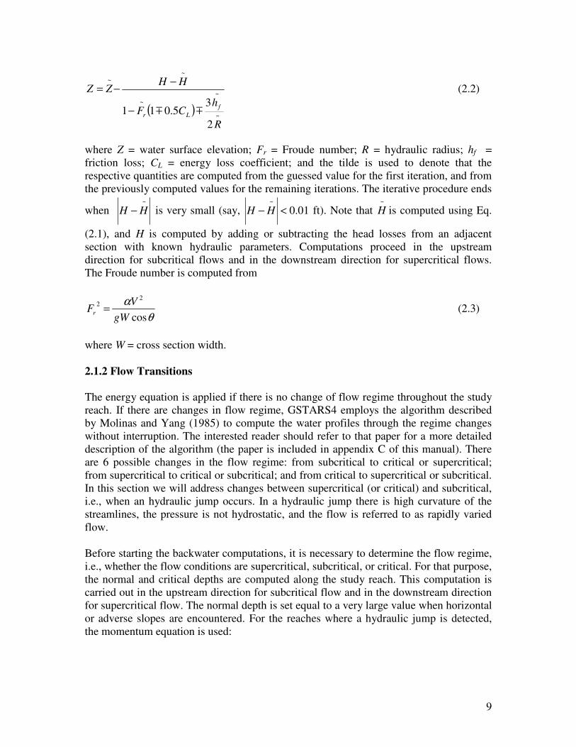
Eq. (2.1) is solved using a trial-and-error procedure based on the standard step method
(Henderson, 1966). The initial surface elevation is guessed, and that guess is iteratively
improved by using
9
( )~
~
~
~~
2
35.011
R
hCF
HHZZ
f
Lr mm−
−−= (2.2)
where Z = water surface elevation; Fr = Froude number; R = hydraulic radius; hf =
friction loss; CL = energy loss coefficient; and the tilde is used to denote that the
respective quantities are computed from the guessed value for the first iteration, and from
the previously computed values for the remaining iterations. The iterative procedure ends
when ~
HH − is very small (say, 01.0~
<− HH ft). Note that ~
H is computed using Eq.
(2.1), and H is computed by adding or subtracting the head losses from an adjacent
section with known hydraulic parameters. Computations proceed in the upstream
direction for subcritical flows and in the downstream direction for supercritical flows.
The Froude number is computed from
θ
α
cos
22
gW
VFr = (2.3)
where W = cross section width.
2.1.2 Flow Transitions
The energy equation is applied if there is no change of flow regime throughout the study
reach. If there are changes in flow regime, GSTARS4 employs the algorithm described
by Molinas and Yang (1985) to compute the water profiles through the regime changes
without interruption. The interested reader should refer to that paper for a more detailed
description of the algorithm (the paper is included in appendix C of this manual). There
are 6 possible changes in the flow regime: from subcritical to critical or supercritical;
from supercritical to critical or subcritical; and from critical to supercritical or subcritical.
In this section we will address changes between supercritical (or critical) and subcritical,
i.e., when an hydraulic jump occurs. In a hydraulic jump there is high curvature of the
streamlines, the pressure is not hydrostatic, and the flow is referred to as rapidly varied
flow.
Before starting the backwater computations, it is necessary to determine the flow regime,
i.e., whether the flow conditions are supercritical, subcritical, or critical. For that purpose,
the normal and critical depths are computed along the study reach. This computation is
carried out in the upstream direction for subcritical flow and in the downstream direction
for supercritical flow. The normal depth is set equal to a very large value when horizontal
or adverse slopes are encountered. For the reaches where a hydraulic jump is detected,
the momentum equation is used:
10
( ) fg FWppVVg
Q−+−=− θββ
γsin211122 (2.4)
where γ = unit weight of water; β = momentum coefficient; p = pressure acting on a
given cross section; Wg = weight of water enclosed between sections 1 and 2; θ = angle of
inclination of channel; and Ff = total external friction force acting along the channel
boundary. If the value of θ is small ( 0sin ≅θ ) and if β1= β2 = 1, Eq. (2.4) becomes
22
2
2
11
1
2
yAgA
QyA
gA
Q+=+ (2.5)
where y = depth measured from water surface to the centroid of the cross section
containing flow. Eq. (2.5) is solved by an iterative trial-and-error procedure.
2.1.3 Normal, Critical, and Sequent Depth Computations
Detailed procedures for normal, critical, and sequent depth computations can be found in
open channel hydraulics books (e.g., Chow, 1959; Henderson, 1966) and are given here
for completeness. The normal depth is computed by satisfying the equation
0)()( 0 =−= SYKQDg (2.6)
where K(Y) = conveyance, which is a function of the depth Y; and S0 = bottom slope.
For adverse and horizontal slopes, the normal depth is set to a very high value.
Critical depth occurs where the Froude number has a value of 1 for a given discharge. In
GSTARS3 and GSTARS4, the critical depth is calculated by satisfying equation
0)(
)()(1)(
3
2
=−=YgA
YWQYDF vα (2.7)
where W(Y) = channel's top width at a depth Y; and A(Y) = channel cross-sectional area at
depth Y.
Sequent depths for a given discharge are the depths with equal specific forces. The
specific force of a natural channel can be expressed by
yAgA
QYSF m
t
+=2
)( (2.8)
where SF(Y) = specific force corresponding to a water depth Y; At = total flow area; and
Am = flow area in which motion exists. In GSTARS3 and GSTARS4, the sequent depth is
computed where hydraulic jumps occur. An iterative trial-and-error procedure is used to

11
find the sequent water surface elevation. The process starts with two guesses: the critical
water surface elevation with the theoretical minimum specific force, and the maximum
bottom elevation for the cross section. The subcritical sequent water surface elevation is
located within these two values. The bisection method is used to solve equation
0)()( =− ba ZSFZSF (2.9)
where Za = computed supercritical water surface elevation, and Zb = desired subcritical
sequent water surface elevation.
2.1.4 Model Representation
In GSTARS4, as in most one-dimensional numerical models, the representation of the
region of the watercourse to be modeled is made by discrete cross sections located at
specific points throughout the river channel (see figure 2.3). The region between each
cross section is called a reach.
Figure 2.3 Conceptual representation of a river reach by discrete cross sections in
GSTARS4
GSTARS4 uses information associated with each cross section to compute the water
surface profiles (and the bed changes in movable bed rivers, as described in the next
chapter). The water surface elevation is computed at each cross section location, but not
between cross sections. Therefore, choosing the appropriate cross section location is very
important. Some guidance is given in the next sections on how to optimize a data
collection program for computer modeling with GSTARS4.
(a) Description of Cross Sections
When setting up a GSTARS4 simulation, the first step is usually the definition and input
of the desired channel reach geometry. This is accomplished by selecting cross sections
along the channel reach. Each cross section is identified by a number that represents its
location expressed as a distance from a downstream reference station. This allows the
12
computer to have a clear representation of the upstream/downstream relationship among
the cross sections, as well as to compute reach lengths (∆x in figure 2.3).
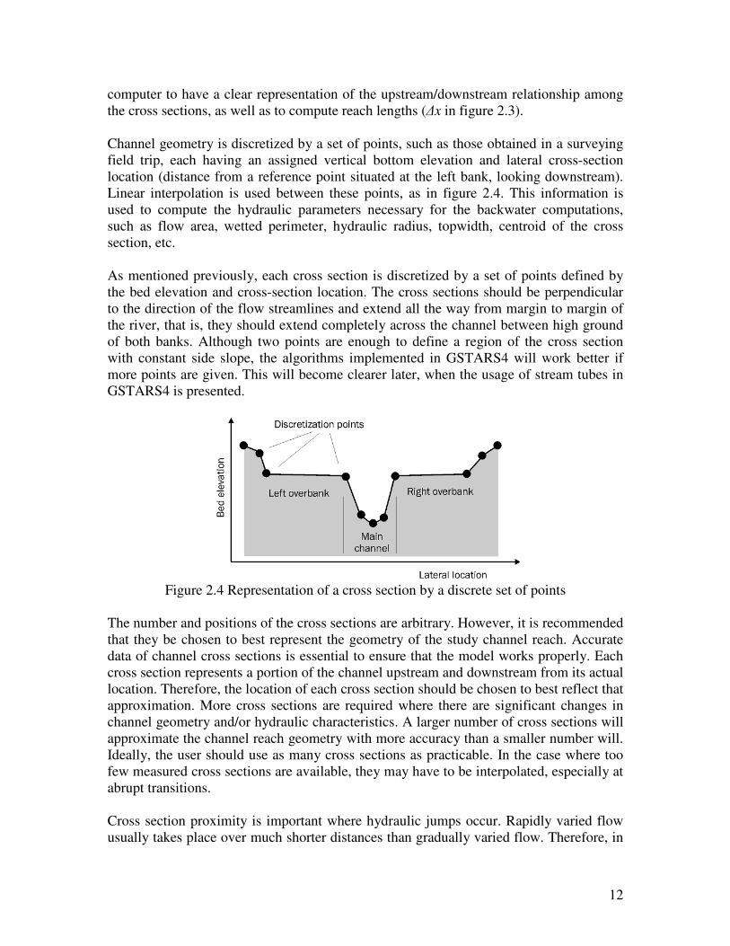
Channel geometry is discretized by a set of points, such as those obtained in a surveying
field trip, each having an assigned vertical bottom elevation and lateral cross-section
location (distance from a reference point situated at the left bank, looking downstream).
Linear interpolation is used between these points, as in figure 2.4. This information is
used to compute the hydraulic parameters necessary for the backwater computations,
such as flow area, wetted perimeter, hydraulic radius, topwidth, centroid of the cross
section, etc.
As mentioned previously, each cross section is discretized by a set of points defined by
the bed elevation and cross-section location. The cross sections should be perpendicular
to the direction of the flow streamlines and extend all the way from margin to margin of
the river, that is, they should extend completely across the channel between high ground
of both banks. Although two points are enough to define a region of the cross section
with constant side slope, the algorithms implemented in GSTARS4 will work better if
more points are given. This will become clearer later, when the usage of stream tubes in
GSTARS4 is presented.
Figure 2.4 Representation of a cross section by a discrete set of points
The number and positions of the cross sections are arbitrary. However, it is recommended
that they be chosen to best represent the geometry of the study channel reach. Accurate
data of channel cross sections is essential to ensure that the model works properly. Each
cross section represents a portion of the channel upstream and downstream from its actual
location. Therefore, the location of each cross section should be chosen to best reflect that
approximation. More cross sections are required where there are significant changes in
channel geometry and/or hydraulic characteristics. A larger number of cross sections will
approximate the channel reach geometry with more accuracy than a smaller number will.
Ideally, the user should use as many cross sections as practicable. In the case where too
few measured cross sections are available, they may have to be interpolated, especially at
abrupt transitions.
Cross section proximity is important where hydraulic jumps occur. Rapidly varied flow
usually takes place over much shorter distances than gradually varied flow. Therefore, in
13
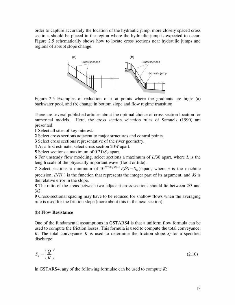
order to capture accurately the location of the hydraulic jump, more closely spaced cross
sections should be placed in the region where the hydraulic jump is expected to occur.
Figure 2.5 schematically shows how to locate cross sections near hydraulic jumps and
regions of abrupt slope change.
Figure 2.5 Examples of reduction of x at points where the gradients are high: (a)
backwater pool, and (b) change in bottom slope and flow regime transition
There are several published articles about the optimal choice of cross section location for
numerical models. Here, the cross section selection rules of Samuels (1990) are
presented:
1 Select all sites of key interest.
2 Select cross sections adjacent to major structures and control points.
3 Select cross sections representative of the river geometry.
4 As a first estimate, select cross section 20W apart.
5 Select sections a maximum of 0.2Y/Sw apart.
6 For unsteady flow modeling, select sections a maximum of L/30 apart, where L is the
length scale of the physically important wave (flood or tide).
7 Select sections a minimum of )/(10 )(log
W
ZINTSS −− δε apart, where ε is the machine
precision, INT( ) is the function that represents the integer part of its argument, and δS is
the relative error in the slope.
8 The ratio of the areas between two adjacent cross sections should lie between 2/3 and
3/2.
9 Cross-sectional spacing may have to be reduced for shallow flows when the averaging
rule is used for the friction slope (more about this in the next section).
(b) Flow Resistance
One of the fundamental assumptions in GSTARS4 is that a uniform flow formula can be
used to compute the friction losses. This formula is used to compute the total conveyance,
K. The total conveyance K is used to determine the friction slope Sf for a specified
discharge:
2
=
K
QS f (2.10)
In GSTARS4, any of the following formulae can be used to compute K:
14
Manning's formula:
2/13/22/1 49.1ff SAR
nKSQ
== (2.11)
Chézy’s formula
( ) 2/12/12/1
ff SCARKSQ == (2.12)
or Darcy-Weisbach’s formula
2/1
2/1
2/1 8ff SA
f
gRKSQ
== (2.13)
where n, C, f = roughness coefficients in Manning, Chézy, and Darcy-Weisbach's
formulae, respectively; g = acceleration due to gravity; A = cross-sectional area; and R =
hydraulic radius.
For each cross section, the desired roughness coefficients are assigned to different
regions of the cross section. Using the example in figure 2.4, the left overbank could have
one value, the main channel another value, and the right overbank yet another value. The
conveyance of each section is computed separately and the total conveyance is taken to
be the sum of the individual conveyances. This method is geared towards natural river
cross-sectional geometries with large width-to-depth ratios, and it may introduce errors in
the water surface elevations in narrow, rectangle-like cross sections.
Estimating roughness is not a trivial task and requires considerable judgment. There are
published flow resistance formulae that are more or less successful when applied to
specific situations, but their lack of generality precludes its use in a numerical model for
broad applications. See, for example, Klaassen et al. (1986) for more details. Some help
exists in the form of tables, such as the ones that can be found in Chow (1959) and
Henderson (1966). Barnes (1967) provides a photographic guide. The method by Cowan
(1956) is summarized here. The basis of this method is on selecting a basic Manning’s n
value from a short set and to apply modifiers according to the different characteristics of
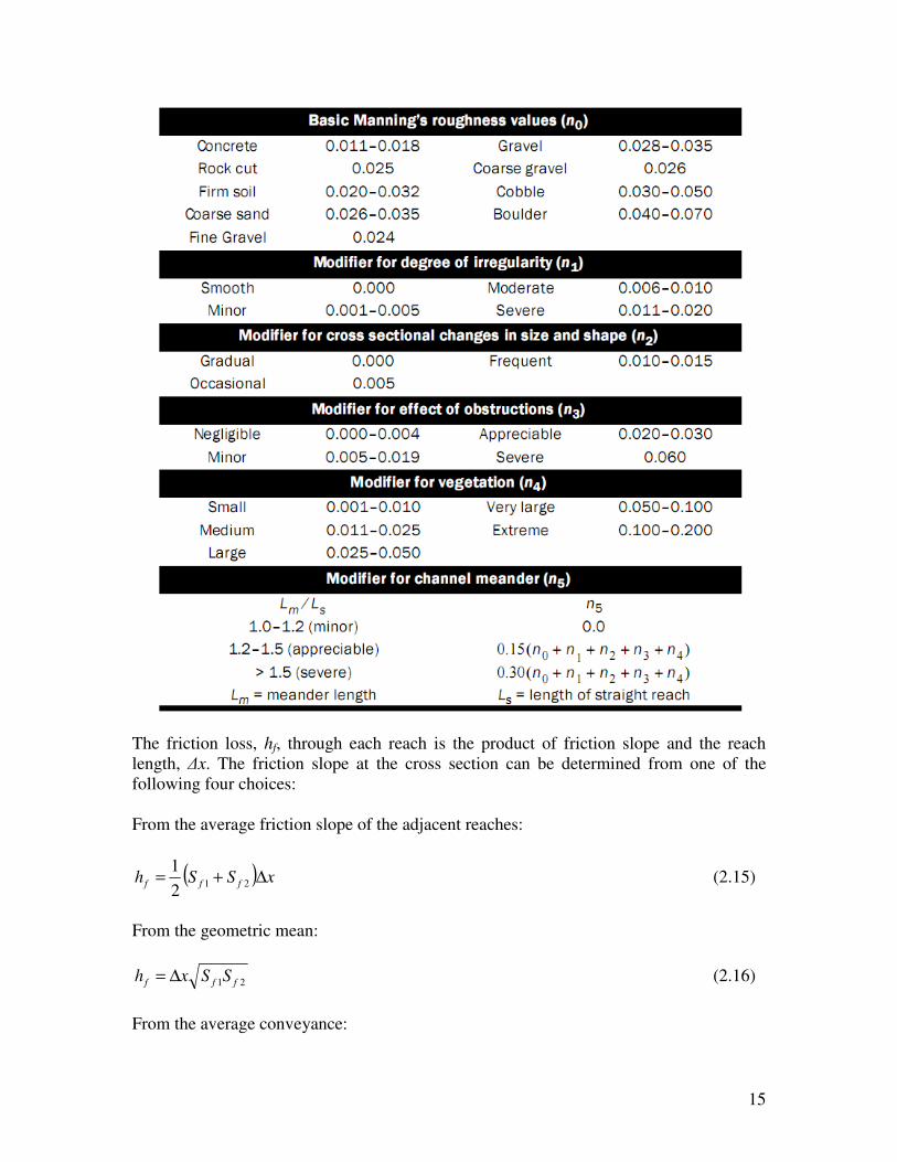
the channel. The method can be applied in steps, with the help of table 2.1:
(1) Select a basic n0.
(2) Add a modifier n1 for roughness or degree of irregularity.
(3) Add a modifier n2 for variations in size and shape of the cross section.
(4) Add a modifier n3 for obstructions (debris, stumps, exposed roots, logs,...).
(5) Add a modifier n4 for vegetation.
(6) Add a modifier n5 for meandering.
The final value of the Manning’s n is given by
543210 nnnnnnn +++++= (2.14)
Table 2.1 provides modifiers for basic Manning’s n in the method by Cowan (1956) with
modifications from Arcement and Schneider (1987).
15
The friction loss, hf, through each reach is the product of friction slope and the reach
length, ∆x. The friction slope at the cross section can be determined from one of the
following four choices:
From the average friction slope of the adjacent reaches:
( ) xSSh fff ∆+= 212
1 (2.15)
From the geometric mean:
21 fff SSxh ∆= (2.16)
From the average conveyance:
16
xLKK
Qh f ∆
+=
2
21
2 (2.17)
From the harmonic mean:
xSS
SSh
ff
ff
f ∆
+=
21
212 (2.18)
Although other choices exist for calculating the friction slope, they are not recommended
- see, for example, Reed and Wolfkill (1976).
The distance between discretized cross sections (the reach length) is important for proper
convergence and accuracy of the methods used in the model. In practice, the reach length
used will vary from case to case. A small, nonuniform channel may require much shorter
reach lengths than a large, uniform channel with mild slopes. A reach length may be
measured along the center line in an artificial channel, along the thalweg in a natural
channel, or along the flow path in overbank areas. Note that, for a given reach of a
channel, these lengths may vary. However, reach lengths may be optimized by using an
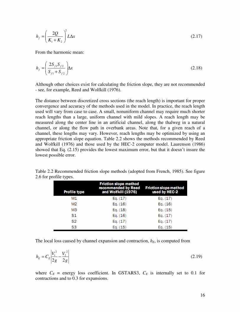
appropriate friction slope equation. Table 2.2 shows the methods recommended by Reed
and Wolfkill (1976) and those used by the HEC-2 computer model. Laurenson (1986)
showed that Eq. (2.15) provides the lowest maximum error, but that it doesn’t insure the
lowest possible error.
Table 2.2 Recommended friction slope methods (adopted from French, 1985). See figure
2.6 for profile types.
The local loss caused by channel expansion and contraction, hE, is computed from
g
V
g
VCh EE
22
2
2
2
1 −= (2.19)
where CE = energy loss coefficient. In GSTARS3, CE is internally set to 0.1 for
contractions and to 0.3 for expansions.
17
Other local losses, such as losses due to channel bends or man-made constructions, are
computed from
g
VCh BB
2
2
2= (2.20)
where CB is an energy loss coefficient supplied by the user. For most natural rivers, CB
values are assumed to be zero. The total energy loss between two adjacent cross sections
is the sum of friction loss and the local losses.
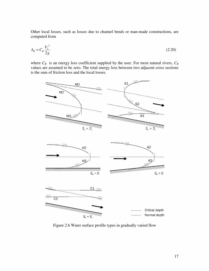
Figure 2.6 Water surface profile types in gradually varied flow

18
2.1.5 Tributary Influence
2.1.5.1 Table Form of Inflow from Tributaries
Although GSTARS4 is limited to single stem rivers, it is possible to include the
contributions of water and sediment by tributaries into the modeled reach. At channel
junctions (see figure 2.7) continuity requires that
BAC QQQ += (2.21)
Figure 2.7 Channel junction
Let cross section B be located at the tributary, and cross sections A and C represent the
computational cross sections used to model the tributary effects. Conservation of energy
is used, i.e.,
f
c
v
A
v hg
VYz
g
VYz +
++=
++
22
22
αα (2.22)
The energy losses, hf, are computed from friction alone, i.e., losses due to bends,
contraction/expansion losses, and user defined values are ignored. (See section 2.1 and
following for details.) A more complete description of this approach to computing flow
across channel junctions can be found in many standard textbooks, for example, Cunge et
al. (1980).
2.1.5.2 Interchanges between a Tributary and the Main Stream
GSTARS4 can simulate water and sediment inflow from tributaries. Not only water and
sediment inflow from tributaries but also the volume of a tributary should be considered.
If the volume of tributaries are not negligible compared to the total volume of the main
stream, volume of tributaries should be included in the simulation. If the inflow of water
and sediment of tributaries are very small, compared with those in the main stream, the
inflow may be ignored for the routing. The “level pool” concept as shown in figure 2.8 is
used to determine the reservoir volume and discharge of tributaries.

19
Figure 2.8 Delineation of volumes to build the capacity table for tributaries
During water surface rising stage at the main channel, water flows to tributaries. In other
words, direction of lateral flow is from the main stream to tributaries. On the other hand,
when water surface draws down, discharge in the reservoir increases because volume of
water in tributaries decreases.
GSTARS4 can simulate water and sediment inflow from tributaries and outflow into
them. It is required that the amount of water and sediment inflow and outflow with
respect to time are provided. In other words, water and sediment discharge table with
respect to time, such as hydrograph, should be provided for a given duration. The
important aspect is to consider the volume of water and sediment in tributaries. Therefore,
tributary impact should be considered with respect to water stage change.
The following simplified assumptions are used for the routing to simulate the interchange
of water and sediment between the main stream and a tributary:
1. The tributary mouth bed elevation is the same as that of the main channel at the
mouth of the tributary.
2. The sediment concentration and size distribution of a tributary is the same as that
in the main stream at the mouth of the tributary.
3. During water surface elevation falling stage in the main channel, tributary water
and sediment will be discharged into the main stream.
4. During the sedimentation or silting stage when the main channel water surface
elevation is rising, water and sediment will flow into tributaries.
5. The main channel and tributary water surface is horizontal and the discharge of
water and sediment into the main river from a tributary is
20
tVolQ ∆∆−=∆ / (2.23)
where Q∆ = water discharge from a tributary to the main river; =∆Vol change of
tributary volume due to the change of the main channel elevation in time t∆ as illustrated
in figure 2.8. The volume of a tributary depends on water stage and bed elevation at the
mouth. Therefore the volume can be computed as follows. b
bhhaVol )( −= (2.24)
where Vol = volume of water in a tributary; h = water surface; bh = bed elevation at a
tributary mouth; and a and b = coefficients of a tributary.
The value of Q∆ is positive when the water of a tributary is discharged into the main
channel during the flushing or water surface elevation falling period. The value of Q∆ is
negative when water is discharged from the main stream to a tributary during the
sedimentation or filling period when the main channel water elevation is rising. Sediment
load to and from a tributary is
ss QCQ ∆=∆ (2.25)
where =∆ sQ sediment load from or into a tributary; and sC = sediment concentration at
the mouth of a tributary.
To compute Q∆ , water surface elevation should be determined first. The main river
routing should be carried out first to determine water surface elevation and sediment
concentration at the mouth of each tributary without considering tributaries. Using water
surface elevations at the mouth of each tributary, Q∆ and sQ∆ of each one are calculated.
After these processes, main channel routing must be redone to calculate sediment
transport and update bed elevation in the main channel using Q∆ and sQ∆ . This
procedure of tributary inflow and outflow computation, which is not included in the
previous GSTARS3, is added to GSTARS4.
2.2 Unsteady Computation
GSTARS4 has the capability to simulated unsteady state flows. Unsteady scheme is
adopted from SRH-1D with minor revisions. The theoretical back ground used for
development of GSTARS4 are based on that of SRH-1D and most of the expressions for
this section are directly referring User’s Manual of SRH-1D (Huang and Greimann,
2007).
2.2.1 Governing Equations
The continuity equation of one-dimensional flow is
( )lat
d qx
Q
t
AA=
∂
∂+
∂
+∂ (2.26)
The momentum equation is
( )fgAS
x
ZgA
x
AQ
t
Q−=
∂
∂+
∂
∂+
∂
∂ /2β (2.27)
where Ad = ineffective cross section area; qlat = lateral inflow per unit length of channel; t
= time; and x = length along the flow direction.

21
2.2.2 Numerical Scheme The discretization of the continuity equation is made with one A-point and two Q-points
giving the difference equation
( )ii
i
n
di
n
i
n
di
n
i QQx
tAAAA −
∆
∆−=−−+ +
−−
1
11 (2.28)
where the overbars signify a time weighted averaged value with a weighting factor
θ ( 10 << θ ) in the time domain. The time weighted discharges, i
Q , can be written as
1)1( −−+= n
i
n
iiQQQ θθ (2.29)
and Eq. (2.28) can be written in an iteration form, with m signifying the iteration number
i
m
ii
m
ii
m
i QQA γδϕ +∆+∆=∆ +1 (2.30)
where the coefficients are
i
ix
t
∆
∆=
θϕ (2.30a)
i
ix
t
∆
∆−=
θδ (2.30b)
( )i
ii
n
di
n
i
n
di
n
iix
tQQAAAA
∆
∆−+++−−= +
−−1
11γ (2.30c)
The discrete form of the momentum equation is made with two A-points and three Q-
points with a weighting factor θ in the time domain giving the difference equation
( )
−
∆
++∆=−
∆
∆+−
−−−fi
i
iiiiwe
i
n
i
n
i Ss
ZZAAtgFF
s
tQQ
111
2 (2.31)
where ( )
i
iie
A
QQF
4
2
1++= β (2.31a)
( )1
2
1
4 −
−+=
i
iiw
A
QQF β (2.31b)
( )2
1
4
−+=
ii
ii
fi
KK
QQS (2.31c)
SRH-1D provides various options for the treatment of the convective terms and
GSTARS4 also has the same options.
Using a weighting factor θ in the time domain, Eq. (2.32) can be written in iteration
form
22
( )
−
∆
++∆+−
∆
∆−+−=
∆∂
∂−∆
∂
∂−
∆∂
∂−
∆
∆−
∆
∆
+∆−
−
∆
−∆+∆∆−
∆∂
∂−∆
∂
∂−∆
∂
∂−
∆∂
∂+∆
∂
∂+∆
∂
∂
∆
∆+∆
−−−
−
−
++−
−
−
+++
−−
−
−
−
−
+
+
fi
i
iiiiwe
i
n
i
n
i
m
in
i
fim
in
i
fi
m
in
i
fi
i
n
i
m
i
i
n
i
m
i
ii
n
fi
i
n
i
n
i
m
i
m
i
m
in
i
em
in
i
wm
in
i
w
m
in
i
em
in
i
em
in
i
e
i
m
i
Ss
ZZAAtgFF
s
tQQ
SA
A
S
AA
S
sT
A
sT
A
AAtg
Ss
ZZAAtg
AA
FQ
Q
FQ
Q
F
AA
FQ
Q
FQ
Q
F
x
tQ
111
1
1
11
1
1
1
111
11
1
1
1
1
1
1
2
2
2
θ
θ
θ
(2.32)
Substituting Eq. (2.30) into Eq. (2.32), results in
i
m
ii
m
ii
m
ii dQcQbQa =∆+∆+∆ +− 11 (2.33)
where the coefficients are
∂
∂−
∆
++−
∆
−∆−
∂
∂−
∂
∂−
∆
∆=
−−
−++
−−
−
−−
n
i
fi
i
n
i
ii
fi
i
n
i
n
ii
in
i
w
n
i
w
i
i
A
S
sT
AAS
s
ZZtg
A
F
Q
F
s
ta
11
111
11
1
11
1
22
θϕ
ϕθ
(2.33a)
( )
( )
∂
∂−
∂
∂−
∆
−+
∂
∂−
∆+
∆−
−
∆
−+
∆−
∂
∂−
∂
∂−
∂
∂+
∂
∂
∆
∆+=
−−
−
−
−−
−
−
n
i
fi
n
i
fi
i
n
i
i
n
i
fi
i
n
i
i
ii
fi
i
n
i
n
iii
in
i
w
n
i
w
in
i
e
n
i
e
i
i
Q
S
A
S
sT
A
S
sTAA
tg
Ss
ZZtg
A
F
Q
F
A
F
Q
F
s
tb
1
1
2
2
1
11
1
1
11
1
1
ϕ
δ
θ
δϕθ
δϕθ
(2.33b)
∂
∂−
∆
−++
−
∆
−∆−
∂
∂+
∂
∂
∆
∆=
−−
+
n
i
fi
ii
ii
fi
i
n
i
n
ii
n
i
e
n
i
e
i
i
A
S
sT
AAS
s
ZZtg
A
F
Q
F
s
tc
1
22
11
1
δθ
δθ
(2.33c)
23
( )
( )
∂
∂−
∆+
∂
∂−
∆+
∆+
−
∆
−+++
∆+
∂
∂+
∂
∂−−
∆
∆+
−=
−−
−−
−
−−
−
−
−
n
i
fi
i
n
i
n
i
fi
i
n
i
iii
fi
i
n
i
n
i
iiii
n
i
w
in
i
e
iew
i
n
i
n
ii
A
S
sTA
S
sTAA
tg
Ss
ZZAA
tg
A
F
A
FFF
s
t
QQd
11
2
2
1
11
11
1
11
1
1
1
γγθ
θγθγ
θγθγ
(2.33d)
where T is the flow top width. For a single channel with N+1 cross sections, there are
N+2 unknowns and N equations from Eqs. (2.33) – (2.33d). One upstream and one
downstream boundary condition are therefore required.
GSTARS4 offers two options, adopted from SRH-1D, for the simulation of supercritical
flow. The options use the Local Partial Inertia (LPI, from Fread and Lewis, 1998)
technique to compute the flow. The LPI technique consists of multiplying the convective
terms by a parameter, σ, as follows,
( )fgAS
x
ZgA
x
AQ
t
Q−=
∂
∂+
∂
∂+
∂
∂ /2βσ (2.34)
( )rFf=σ (2.35)
GSTARS4 has two methods to compute the function ( )rFf ,
( )51,0max
−−= rFσ (2.36)
or
( )2,1min
−= rFσ (2.37)
Eq. (2.36) is taken from FLDWAV (Fread and Lewis, 1998) and Eq. (2.37) is taken from
MIKE 11 (DHI software, 2002). The function from FLDWAV provides damping of the
convective terms for Fr < 1, while the function from MIKE 11 does not damp the
convective term until Fr > 1. The function from FLDWAV will be generally more stable,
but the function from MIKE 11 will be generally more accuate. Neither method will
accurately simulate the propagation of rapid changing hydrographs that occurs during
dam break. In addition, neither method will calculate the location of hydraulic jumps
accurately. Regardless of the method of solutions, GSTARS4 and SRH-1D assumes that
subcritical flow occurs at the boundaries of a river.
24
CHAPTER
3
SEDIMENT ROUTING AND
CHANNEL GEOMETRY ADJUSTMENT
Sediment transport occurs when the flow exceeds a certain threshold and becomes
capable of moving the particles that constitute the bed. When the channel’s bed becomes
mobile, erosion or deposition may occur. These bed changes depend on many parameters,
including hydraulic conditions (such as flow velocity and depth), bed composition (such
as size of the particles that constitute the bed), and supply rates (amount and type of
sediments entering the channel). In this chapter, the sediment transport and bed evolution
model employed by GSTARS4 is presented with some detail.
From the user point of view, the backwater and the sediment transport computations can
be viewed as two modules belonging to the same numerical model. The backwater
module can be used without the need to use the sediment transport module. For fixed bed
channels (such as the flow of clear water over lined channels or spillways), the sediment
transport computations can be turned off, reducing the data requirements of the model
(the description of the bed composition) and allowing faster set-up and shorter run times.
The user wishing to employ GSTARS4 to fixed bed channels can safely skip chapters 3
and 4 of this manual.

25
3.1 Governing Equations
3.1.1 Theoretical Background
It is convenient to distinguish two main types of transportation of sediments: in
suspension in the water column, and as bed load. The particles in motion that remain
close to the channel’s bed are said to belong to the bed load. These particles move by
rolling over the bed and by saltating over relatively short lengths, and constitute a layer of
relatively small thickness. In contrast, the particles transported in suspension may span
the entire water column above the bed load layer. They are transported by the turbulent
forces of the fluid, i.e., the turbulent eddies, and are generally of smaller dimensions than
the particles in the bed load. These two layers have different composition and move at
different speeds.
The distinction between the two layers is problematic and it is not easy to locate a clear
interface at a certain elevation above the bed. The difficulties are compounded by the fact
that there is a continuous exchange of particles between the bed load layer and the
suspended load. Furthermore, the separation of the two layers requires distinct governing
equations for each layer, each with its own sets of variables and coefficients, some of
which are very difficult to determine.
An alternate approach lumps the suspended load and the bed load together in what is
called the bed-material load. This eliminates the need to describe the interface between
the bed load and the suspended load and the sediment fluxes crossing it, which is difficult
and, with the present state-of-the-art, imprecise. It also is computationally more efficient,
since that a fewer number of equations needs to be solved. Consequently, the bed-
material load approach requires less data, some of which is very difficult to obtain (such
as the diffusion coefficients necessary to compute the transport of suspended load). The
trade-off is in the loss of accuracy, since this approach does not distinguish the two
essentially different modes of transport. In GSTARS4 the bed-material load approach
was chosen to describe the transport of sediments.
3.1.2 Sediment Continuity Equation
The basis for sediment routing computations in GSTARS4 is the conservation of
sediment mass. In one-dimensional unsteady flow, the sediment continuity equation can
be written as
0=−∂
∂+
∂
∂+
∂
∂lat
sds qt
A
t
A
x
Qη (3.1)
where η = volume of sediment in a unit bed layer volume (one minus porosity); Ad =
volume of bed sediment per unit length; As = volume of sediment in suspension at the
cross section per unit length; Qs = volumetric sediment discharge; and qlat = lateral
sediment inflow. A number of assumptions are made to simplify this equation.
Firstly, it is assumed that the change in suspended sediment concentration in a cross
section is much smaller than the change of the river bed, i.e.:

26
t
A
t
A ds
∂<<
∂
∂η (3.2)
Secondly, during a time step, the parameters in the sediment transport function for a cross
section are assumed to remain constant:
0=∂
∂
t
Qs or dx
dQ
x
Q ss =∂
∂ (3.3)
With these assumptions, Eq. (3.1) becomes
latsd q
x
Q
t
A=
∂
∂+
∂
∂η (3.4)
which is the governing equation used in GSTARS4 for routing sediments in rivers and
streams.
3.2 Streamlines and Stream Tubes
GSTARS4 routes sediments using stream tubes. The basic concept and theory regarding
streamlines, stream tubes, and stream functions can be found in most basic text books of
fluid mechanics. In this section, only some of the basic concepts are given, as they are
applied in the model.
By definition, a streamline is a conceptual line to which the velocity vector of the fluid is
tangent at each and every point, at each instant in time. Stream tubes are conceptual tubes
whose walls are defined by streamlines. The discharge of water is constant along a stream
tube because no fluid can cross the stream tube boundaries. Therefore, the variation of the
velocity along a stream tube is inversely proportional to the stream tube area. Figure 3.1
illustrates the basic concept of stream tubes used in GSTARS4.
For steady and incompressible fluids, the total head, tH , along a stream tube of an ideal
fluid is constant:
==++ tHhg
Vp
2
2
γConstant (3.5)
where p = pressure acting on the cross section; γ = unit weight of water; V = velocity; g =
acceleration due to gravity; and h = hydraulic head. In GSTARS4, however, Ht is reduced
along the direction of the flow due to friction and other local losses, as described earlier
in section 2.1.1.
In GSTARS4, the backwater profiles are computed first. Then, the cross sections are
divided into several sections of equal conveyance. These regions of equal conveyance are
27
treated as stream tubes, and the (computed) locations of their boundaries are the defining
streamlines, across which no water can pass. The thus defined stream tubes are used as if
they were conventional one-dimensional channels with known hydraulic properties, and
sediment routing can be carried out within each stream tube almost as if they were
independent channels.
Figure 3.1 Schematic representation illustrating the use of stream tubes by GSTARS4
Stream tube locations are computed for each time step, therefore they are allowed to vary
with time. Sediment routing is carried out for each stream tube and for each time step.
Bed material composition is computed for each tube at the beginning of the time step, and
bed sorting and armoring computations are also carried out separately for each stream
tube. In GSTARS4, lateral variations of bed material composition are accounted for, and
this variation is included in the computations of the bed material composition and sorting
for each stream tube. This approach allows the computation of cross-sectional variations
in the hydraulic and sediment parameters in a quasi-two-dimensional manner. For
example, aggradation and degradation can occur simultaneously at a given cross section.
Conventional one-dimensional models are unable to deal with this situation, but
GSTARS4 can model it, since erosion or deposition are computed separately within each
stream tube, depending on the hydraulics, bed composition, transport capacity, and
sediment supply conditions for each stream tube.
The movement of a sediment particle will have a direction which, in general, is neither
the direction of the flow nor the direction of the bed shear stress. For example, in a bend
of a channel with a sloping bed such as the one in figure 3.2, the larger particles will tend
to roll down the slope (gravitational forces dominate) while the smaller particles may
move up the slope (lift forces due to secondary currents dominate) - see, for example,
Ikeda et al., (1987). A non-zero transverse flux results in exchange of sediments across
stream tube boundaries. Note that this exchange does not violate the theoretical

28
assumptions behind the use of stream tubes because the trajectories of the sediment
particles are not the same as the trajectories of the fluid elements (streamlines). Therefore,
although there is no net exchange of water between stream tubes, sediment can cross
stream tube boundaries, and the use of stream tubes may still be theoretically justified.
Figure 3.2 Bed sorting in bends due to transverse bed slope and secondary currents
GSTARS4 includes the effects of stream curvature that contribute to the radial
(transverse) flux of sediments, qr, near the bed. The two effects considered are transverse
bed slope and secondary flows. The effects due to secondary flows are modeled
following Kikkawa et al. (1976), in which the angle that the bed shear stress vector
makes with the downstream direction, β, is given by
+−=
v
u
RAu
vh
r κβ
*
*640.2167.4 (3.6)
where v = average velocity along the channel’s centerline; u*= shear velocity along the
centerline; h = water depth; R = radius of curvature of the channel; Ar = an empirical
coefficient (for rough boundaries Ar = 8.5); and κ = von Karman constant(= 0.41).
In a bed with transverse slope, the gravity forces cause the direction of the sediment
particles to be different from that of the water particles. Following Ikeda et al. (1987), the
effects due to a transverse bed slope can be added to those due to curvature such that
δτ
τ
λµ
αµβσ tan
1tantan
*
*
0++==
s
r
q
q (3.7)
where qs = unit sediment transport rate in the channel’s longitudinal direction; σ = the
angle between the direction of transport and the channel’s downstream direction; *
0τ , *τ =
nondimentional critical shear stress and bed shear stress, respectively; δ = transverse bed
slope; α = rate of lift to drag coefficients on sediment particles (determined
experimentally to be equal to 0.85); λ = sheltering coefficient (= 0.59); and µ = dynamic
Coulomb friction factor (= 0.43). The direction of sediment transport is calculated from
Eq. (3.7). The components of the sediment tranport direction vector are given by
29
σcosts qq = (3.8)
σsintr qq = (3.9)
where qt = sediment transport rate per unit width computed by any of the sediment
transport equations discussed in section 3.5. Eq. (3.4) is then solved using yqQ ss ∆= and
rlat qq = , where ∆y = stream tube width.
Note that the above methods are applied only to sediment moving as bed load. Sediment
moving as suspended load is not allowed to cross stream tube boundaries. GSTARS4
uses van Rijn’s (1984) method to determine if a particle of a given size is in suspension
or moves as bed load:
=*
,scru
*
4
D
sω if 1 < D
* ≤ 10 (3.10)
sω4.0 if D*
>10
where *
,scru = critical shear velocity for suspension; ωs = fall velocity of sediment
particles; and D* = dimensionless grain size defined as
3/1
2
* )1(
−=
ν
gsdD (3.11)
where d = sediment particle diameter; s = specific gravity of sediment in water; g =
acceleration due to gravity; and ν = viscosity of water.
There are some limitations to the use of stream tubes in the manner described in the
present section. Firstly, the backwater curves result from an essentially one-dimensional
model, where the water surface elevation is assumed to be horizontal across each cross
section. Therefore extrapolation to two-dimensional distributions using the described
method has some limitations. Consequently, the maximum recommended number of
stream tubes employed is 5 (this is the maximum number of stream tubes allowed by the
GSTARS4 program). GSTARS4 is not a truly two-dimensional program, therefore it
cannot simulate areas with recirculating flows or eddies. Other limitations include the
inability of simulate secondary flows, reverse flows, water surface variations in the
transverse direction, hydrograph attenuation, and others that result from the use of the
simplified governing equations described in this and the previous chapters.
3.3 Discretization of the Governing Equations
In this section we describe the basic steps to solve Eq. (3.4) numerically. Note that Eq.
(3.4) is a partial differential equation, but that the computer can only solve algebraic
equations. The term discretization means the transformation of the partial differential
equation into a set of algebraic equations that can be solved numerically by a computer.
The numerical solution of differential equations is a very large field of applied

30
mathematics. The reader interested in its particular application to fluid mechanics should
refer to one of many text books dedicated to the subject, such as the ones by Hirsch
(1988) or Anderson et al. (1997), for example.
The approach used in GSTARS4 uses a finite difference uncoupled approach. This means
that finite differences are used to discretize the governing differential equation. By
uncoupled solution it is meant that first the backwater profiles are computed; the
sediment routing and bed changes are computed afterwords, keeping all the hydraulic
parameters frozen during the calculations.
In order to accomplish the discretization process, the change in the volume of bed
sediment due to deposition or scour, ∆Ad, is written as
( ) iiiid ZcTbTaTA ∆++=∆ +− 11 (3.12)
where T = top width; Z = change in bed elevation (positive for aggradation, negative for
scour); i = cross section index; and a, b, and c are constants that must satisfy
a + b + c = 1 (3.13)
There are many possible choices for the values of a, b, and c. For example, a = c = 0 and
b = 1 is a frequently used combination that is equivalent to assuming that the wetted
perimeter at station i represents the perimeter for the entire reach. If b = c = 0.5 and a =
0, emphasis is given to the downstream end of the reach.
In practice, it is observed that giving emphasis to the downstream end of the reach may
improve the stability of the calculations. Such a scheme may be represented by using the
following expressions:
a = 0; b = 1 - θ; and c = θ (3.14)
where θ is a weighting parameter (θ > 0.5). In GSTARS4, the standard values are a = c =
0.25 and b = 0.5, but the user can change those to any combination that satisfies Eq.
(3.13). Using Eq. (3.12), the partial derivative terms are approximated as follows:
( )t
ZcTbTaT
t
A iiiid
∆
∆++≈
∂
∂ +− 11 (3.15)
( )1
1,,
2/1 −
−
∆+∆
−≈
ii
isiss
xx
dx
dQ (3.16)
where ix∆ = distance between cross sections i and i+1; ∆t = time step interval; and Qs,i =
sediment transport rate at cross section i. The sediment continuity equation, Eq. (3.4), can
be used to compute the change in bed elevation, ∆Zi, which is done for each individual
sediment size fraction within each stream tube. Inserting Eqs. (3.15) and (3.16) into Eq.
(3.4) we obtain
31
( ) ( )( )( )111
,,,1,1
,
2
−+−
−−
∆+∆++
−+∆+∆⋅
∆=∆
iiiii
kiskisiilat
i
kixxcTbTaT
QQxxqtZ
η (3.17)
where k = size fraction index; iη = volume of sediment in a unit bed layer at cross section
i; and Qs,i,k = computed volumetric sediment discharge for size class k at cross section i.
The total bed elevation change for a stream tube at cross section i, ∆Zi, is computed from
∑=
∆=∆N
k
kii ZZ1
, (3.18)
where N = total number of size fractions present in cross section i. The new channel cross
section at station i, to be used at the next time iteration, is determined by adding the bed
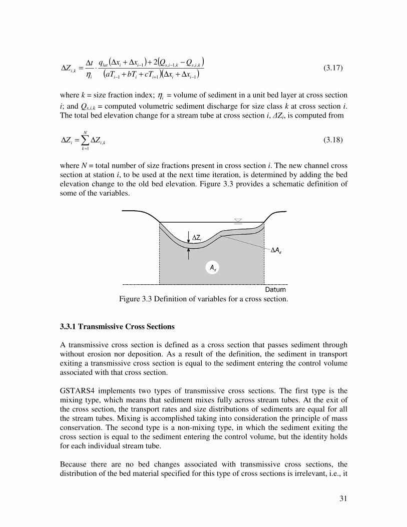
elevation change to the old bed elevation. Figure 3.3 provides a schematic definition of
some of the variables.
Figure 3.3 Definition of variables for a cross section.
3.3.1 Transmissive Cross Sections
A transmissive cross section is defined as a cross section that passes sediment through
without erosion nor deposition. As a result of the definition, the sediment in transport
exiting a transmissive cross section is equal to the sediment entering the control volume
associated with that cross section.
GSTARS4 implements two types of transmissive cross sections. The first type is the
mixing type, which means that sediment mixes fully across stream tubes. At the exit of
the cross section, the transport rates and size distributions of sediments are equal for all
the stream tubes. Mixing is accomplished taking into consideration the principle of mass
conservation. The second type is a non-mixing type, in which the sediment exiting the
cross section is equal to the sediment entering the control volume, but the identity holds
for each individual stream tube.
Because there are no bed changes associated with transmissive cross sections, the
distribution of the bed material specified for this type of cross sections is irrelevant, i.e., it

32
does not impact sediment routing computations. See record ST in appendix A for
instructions on how to use transmissive cross sections in GSTARS4.
3.3.2 Numerical Stability
The formulation described above is subject to numerical stability constraints. A
numerical scheme is said to be stable if, for a certain condition, the solution values
constructed with that scheme remain finite for the set of all solutions that take an initial
state (at t = 0) to its final state (at t = T). The condition for which the solution is stable is
called the Courant-Friedrichs-Lewy, or CFL, condition. The CFL stability condition is
usually expressed via the Courant number
solutionnumericaltheinnpropagatioofcelerity
solutionanalyticaltheinnpropagatioofcelerityCr = (3.19)
so that the CFL condition becomes Cr ≤ 1 for stability. Although implicit schemes are
generally unconditionally stable (i.e., are not restricted by Courant number values),
explicit schemes have stability limits that translate into limits to the maximum size of the
time step. GSTARS4 uses an explicit method to solve the sediment routing equation. In
this case, the CFL stability criterion is given by
sc
xt
∆≤∆ (3.20)
where cs is the kinematic wave speed of the bed changes.
In practice, instability is observed by the presence of spurious oscillations in an otherwise
smooth solution, that is, in the hydraulic parameters and/or bed elevations. These
oscillations are purely of numerical nature, having no physical meaning, and they creep
into the solution as the time step is increased. Their amplitude increases with simulation
time (i.e., with the number of time steps) and eventually causes the computations to stop
prematurely due to numerical errors. This phenomenon can be avoided by reducing the
time step until the CFL condition is met. In general, the time step has to be smaller when
the computational cross sections are placed closer together, and vice versa. Numerical
experimentation is required to determine a suitable value for ∆t.
3.3.3 Additional Comments
The solution procedure used by GSTARS4 decouples the governing equation for the flow
from the governing equation for the sediment routing. For each time step, the backwater
computations are solved first. The hydraulic properties are then assumed constant for the
remainder of the time step. Sediment routing is carried out in this hydraulically “frozen”
state, using a sediment transport formula for steady flow, Eq. (3.3), expresses this
simplification. The change in bed levels are computed from the sediment continuity
equation and are updated before the algorithm proceeds to the next time step. The time
marching proceeds sequentially in this manner, until the desired time is reached.

33
This is the most common type of solution approach in numerical modeling. It requires
that the variations in the sedimentological parameters, such as bed level and composition,
be small when compared to the variation in the hydraulic properties. In general, this can
be accomplished by having a computational time step ∆t that is small enough. One way to
work this out in practice is to have a small enough ∆t such that
ii hZ <<∆ (3.21)
for all the computational cross sections and for all time steps. In Eq. (3.21), hi is the
hydraulic depth of cross section i.
There are other limitations to the uncoupled approach. First, it should not be used in the
region 0.8 < Fr < 1.2, where Fr is the Froude number (see de Vries (1969) for details
about the derivation of this constraint). Second, it does not handle rapidly varying
boundary conditions. The first limitation means that the approach is not valid in flow
regime transitions. However, in nature regime transitions on movable beds do no occur
often, are very localized, and are mostly temporary, therefore this limitation does not
pose a serious obstacle to the use of uncoupled models such as GSTARS4.
The second limitation mentioned was treated by Lyn (1987). He shows that uncoupled
models are limited to the situations were the input hydrograph obeys the following
approximate relationship:
( )100
/≥
VL
T (3.22)
where T = duration of the hydrograph; L = length of the reach being modeled; and V = a
characteristic velocity in the channel. V can be computed from
ghV = (3.23)
where g = acceleration due to gravity, and h = hydraulic depth. Note, however, that the
steady flow part of GSTARS4 is limited to stepped hydrographs, and should not be used
for situations where the unsteady effects are important. In the quasi-steady range of
applications targeted by GSTARS4, it is unlikely that the limitations associated with
uncoupling hydraulics and sediment transport are significant.
3.4 Bed Sorting and Armoring
GSTARS4 computes sediment transport by size fraction. As a result, particles of different
sizes are transported at different rates. Depending on the hydraulic parameters, the
incoming sediment distribution, and the bed composition, some particle sizes may be
eroded, while others may be deposited or may be immovable. GSTARS4 computes the
carrying capacity for each size fraction present in the bed, but the amount of material
actually moved is computed by the sediment routing equation, Eq. (3.4). Consequently,

34
several different processes may take place. For example, all the finer particles may be
eroded, leaving a layer of coarser particles for which there is no carrying capacity. No
more erosion may occur for those hydraulic conditions, and the bed is said to be armored.
This armor layer prevents the scour of the underlying materials and the sediment
available for transport becomes limited to the amount of sediment entering the reach.
However, future hydraulic events, such as an increase of flow velocity, may increase the
flow carrying capacity, causing the armor layer to break and restart the erosion processes
in the reach.
Many different processes may occur simultaneously within the same channel reach.
These depend not only on the composition of the supplied sediment, i.e., the sediment
entering the reach, but also on bed composition within that reach. The bed composition
may vary within the reach both in space and time. In order to model these type of events,
GSTARS4 uses the bed composition accounting procedure proposed by Bennett and
Nordin (1977).
In Bennett and Nordin's method, bed accounting is accomplished by the use of two or
three conceptual layers (three layers for deposition and two layers for scour). The process
is schematically illustrated in figure 3.4. The top layer, which contains the bed material
available for transport, is called the active layer. Beneath the active layer is the inactive
layer, which is the layer used for storage. Below these two layers there is the undisturbed
bed, with the initial bed material composition.
The active layer is the most important concept in this procedure. It contains all the
sediment that is available for transport at each time step. The thickness of the active layer
is defined by the user as proportional to the geometric mean of the largest size class
containing at least 1 percent of the bed material at that location.
Active layer thickness is, therefore, closely related to the time step duration. Erosion of a
particular size class of bed material is limited by the amount of sediments of that size
class present in the active layer. If the flow carrying capacity for a particular size class is
greater than what is available for transport in the active layer, the term availability limited
is used (Bennett and Nordin, 1977). On the other hand, if more material is available than
that necessary to fulfill the carrying capacity computed by a particular sediment transport
equation, the term capacity limited is used.
The inactive layer is used when net deposition occurs. The deposition thickness of each
size fraction is added to the inactive layer, which in turn is added to the thickness of the
active layer. The size composition and thickness of the inactive layer is computed first,
after which a new active layer is recomputed and the channel bed elevation updated.
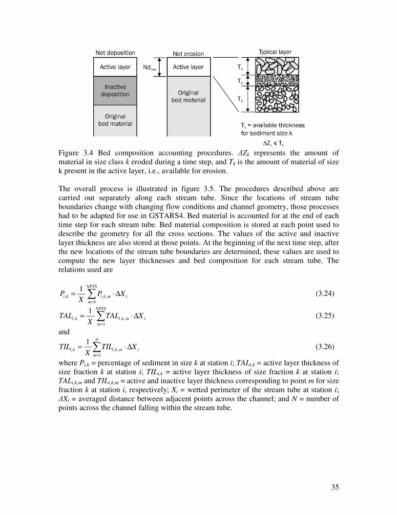
35
Figure 3.4 Bed composition accounting procedures. ∆Zk represents the amount of
material in size class k eroded during a time step, and Tk is the amount of material of size
k present in the active layer, i.e., available for erosion.
The overall process is illustrated in figure 3.5. The procedures described above are
carried out separately along each stream tube. Since the locations of stream tube
boundaries change with changing flow conditions and channel geometry, those processes
had to be adapted for use in GSTARS4. Bed material is accounted for at the end of each
time step for each stream tube. Bed material composition is stored at each point used to
describe the geometry for all the cross sections. The values of the active and inactive
layer thickness are also stored at those points. At the beginning of the next time step, after
the new locations of the stream tube boundaries are determined, these values are used to
compute the new layer thicknesses and bed composition for each stream tube. The
relations used are
∑=
∆⋅=NPTS
m
imkiki XPX
P1
,,,
1 (3.24)
∑=
∆⋅=NPTS
m
imkiki XTALX
TAL1
,,,
1 (3.25)
and
∑=
∆⋅=N
m
imkiki XTILX
TIL1
,,,
1 (3.26)
where Pi,k = percentage of sediment in size k at station i; TALi,k = active layer thickness of
size fraction k at station i; TILi,k = active layer thickness of size fraction k at station i;
TALi,k,m and TILi,k,m = active and inactive layer thickness corresponding to point m for size
fraction k at station i, respectively; Xi = wetted perimeter of the stream tube at station i;
∆Xi = averaged distance between adjacent points across the channel; and N = number of
points across the channel falling within the stream tube.

36
Figure 3.5 Simplified diagram for the bed sorting and armoring processes. Adopted from
Bennett and Nordin (1977), with modifications.
Note that GSTARS4 allows for layered beds, in which each layer contains a different
particle distribution. In the case of multiple bed layers, an average bed composition is
computed from the particle distribution information stored at each point in the cross
section. For example, for the case pictured in figure 3.6, the substratum is composed of
three different layers, each layer with its own sediment particle distribution. For the
conditions shown - and considering only one stream tube, for the sake of brevity - a
weighted average is composed from the particle distributions of layer 1 (points 2 and 7),
layer 2 (points 3 and 6), and layer 3 (points 4 and 5). Points 1, 8, and 9 are above the
water line, therefore they do not contribute to the averaging process. The weighting factor
is given by the percentage of wetted perimeter associated with each discretization point.
37
Figure 3.6 Cross section showing how individual discretization points may have different
sediment particle distributions.
3.4.1 Remarks
For a given time step, erosion of the bed or banks will take place when the sediment
transport capacity at a given cross section exceeds the load incoming from the upstream
cross section. When erosion takes place, sediment transport may be constrained by
availability. The materials available for entrainment are those exposed at the bed surface.
The concept of the active layer is fundamental. The active layer is the surface layer from
which materials can be entrained by the flow. In other words, for each simulation time
step, the only material available for erosion is the sediment contained in the active layer.
Therefore, the active layer thickness, maxNd=δ , should always be at least as thick as the
expected maximum depth of scour (∆Z). The recommended way to achieve this is by
defining the active layer thickness first and then appropriately choosing the time step for
sediment transport calculations (∆ts). A trial-and-error process can be used to ensure that
∆Z ≤ δ.
Alternatively, an estimate of ∆ts can be obtained from a simplified form of Eq. (3.17):
sii
siis
t
Z
Px
∆
∆=
∆
−−
η1,
(3.27)
where ∆Z is prescribed to satisfy the above criterion (i.e., δ≤∆Z ). In this case, the
estimate should be obtained using the peak inflow discharge.
3.5 Sediment Transport Functions
The literature contains many sediment transport functions. Usually, each transport
function was developed for a certain range of sediment size and flow conditions.
Computed results based on different transport functions can differ significantly from each
other and from measurements. No universal function exists which can be applied with
accuracy to all sediment and flow conditions. With the exception of Yang's formulae,
most transport functions are intended for subcritical flows. GSTARS4 has 15 transport
functions for cohesionless material, presented in table 3.1. More detailed descriptions of
these functions were published by Yang (1996, 2003), which also includes a number of
different comparisons and evaluations. None of the transport functions can be applied to
all flow and sediment conditions with accuracy. Yang and Huang (2001) made detailed
analysis and recommendations on the selection of sediment transport functions under
different flow and sediment conditions (Yang and Huang’s paper is presented in appendix
D). Other useful assessments of sediment transport formulae can be found in White et al.
(1975), Alonso (1980), Alonso et al. (1982), ASCE (1982), Vetter (1987, 1988), Gomez
and Church (1989), and Yang and Wan (1991). Some of these analyses rank the
equations by reliability and applicability. Not surprisingly, the ranking is quite different
among the authors.
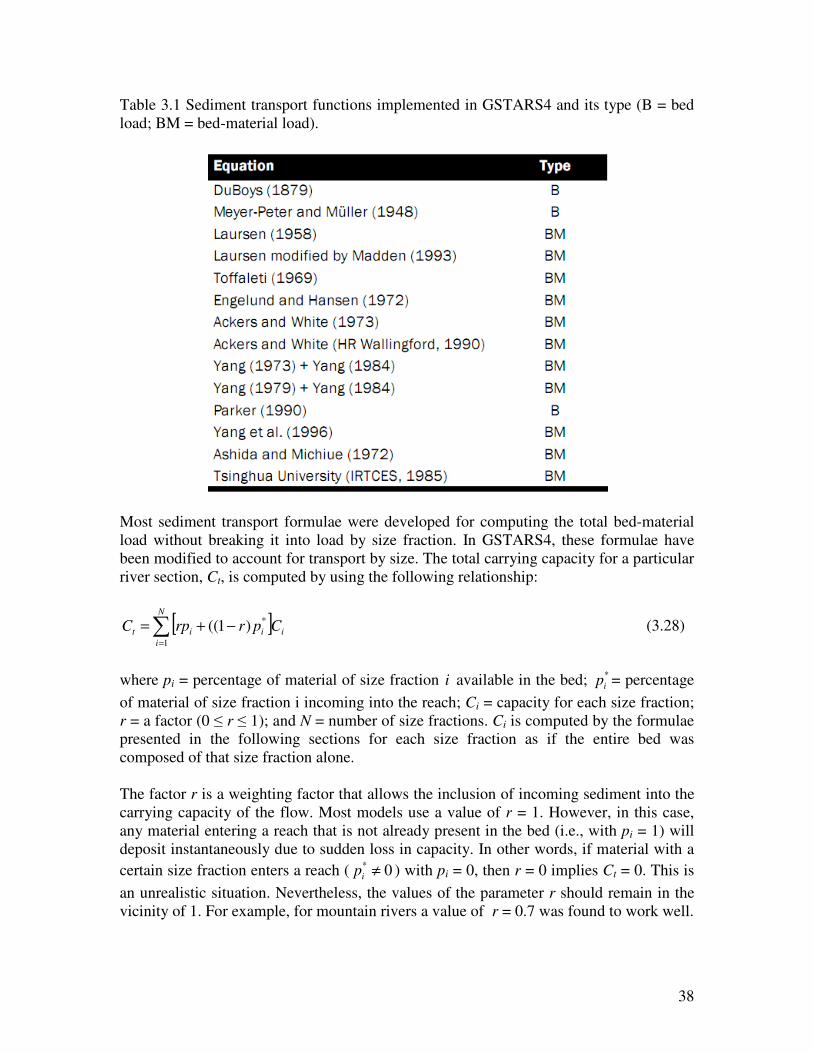
38
Table 3.1 Sediment transport functions implemented in GSTARS4 and its type (B = bed
load; BM = bed-material load).
Most sediment transport formulae were developed for computing the total bed-material
load without breaking it into load by size fraction. In GSTARS4, these formulae have
been modified to account for transport by size. The total carrying capacity for a particular
river section, Ct, is computed by using the following relationship:
[ ]∑=
−+=N
i
iiit CprrpC1
*)1(( (3.28)
where pi = percentage of material of size fraction i available in the bed; *
ip = percentage
of material of size fraction i incoming into the reach; Ci = capacity for each size fraction;
r = a factor (0 ≤ r ≤ 1); and N = number of size fractions. Ci is computed by the formulae
presented in the following sections for each size fraction as if the entire bed was
composed of that size fraction alone.
The factor r is a weighting factor that allows the inclusion of incoming sediment into the
carrying capacity of the flow. Most models use a value of r = 1. However, in this case,
any material entering a reach that is not already present in the bed (i.e., with pi = 1) will
deposit instantaneously due to sudden loss in capacity. In other words, if material with a
certain size fraction enters a reach ( 0* ≠ip ) with pi = 0, then r = 0 implies Ct = 0. This is
an unrealistic situation. Nevertheless, the values of the parameter r should remain in the
vicinity of 1. For example, for mountain rivers a value of r = 0.7 was found to work well.

39
The hydraulic parameters used to compute the sediment carrying capacities in each reach
are computed as weighted averages from the hydraulic parameters from nearby stations.
For each station i, the representative values of the area (ARi), depth (DRi), velocity (VRi),
and friction slope (SRi) are computed as follows:
11 +− ++= iiiRi cAbAaAA (3.29)
11 +− ++= iiiRi cDbDaDD (3.30)
11 +− ++= iiiRi cVbVaVV (3.31)
11 +− ++= iiiRi cSbSaSS (3.32)
The weighting parameters a, b, and c can be chosen in any combination that satisfies Eq.
(3.13). By default, GSTARS4 assumes the values of a = c = 0 and b = 1, but these values
can be changed by the user. For example, in rivers whose properties change more rapidly
from section to section, a scheme incorporating information from the upstream and
downstream reaches may be more appropriate. The values of a = c = 0.25 and b = 0.5
may be adopted in those circumstances. By changing a, b, and c appropriately, the user
can use the parameters that favor stability or that favor sensitivity. Usually, more
sensitive schemes are the less stable, and vice-versa.
For the station located farthest downstream (station i = NSTA), the values for the
parameters at station i + 1 are not defined; therefore only parameters a and b are
necessary. For that station, GSTARS4 defines a = 0 and b = 1. These values can be
changed by the user. For the example given above, a possible combination of values
might be a = b = 0.5.
For the first upstream station (station i = 1), station i - 1 is not defined, therefore
parameter a is not used. GSTARS4 defaults to b = 1 and c = 0, but these values can be
changed by the user.
Note that the coefficients a, b, and c may be numerically different and are independent
from those used in Eq. (3.12), although they have a similar function.
3.5.1 DuBoys’ Method (1879)
The pioneering work of DuBoys (1879) is based on the premise that the sediment moves
in layers that slide over each other. Although the concept was ultimately proven
unrealistic, it was found that his equation could still be used to describe the data. DuBoys
reached an expression that is based on the excess of shear stress:
( )cb Kq τττ −= (3.33)

40
where qb = bed load discharge by volume per unit channel width; τ = bed shear stress;
and τc = critical tractive force along the bed. τc can be computed from Shields diagram.
Straub (1935) found the following relationship for K:
4/3
173.0
dK = (3.34)
where d = particle size.
3.5.2 Meyer-Peter and Müller's Formula (1948)
The Meyer-Peter and Müller's formula (1948) is a bed load formula for gravel or coarse
materials:
( ) 3/23/1
2/3
25.0047.0 bs
r
s qdK
KRS ργγγ +−=
(3.35)
where γ and γs = specific weights of water and sediment (metric tons/m3), respectively; R
= hydraulic radius (m); S = energy slope; d = mean particle diameter (m); ρ = specific
mass of water (metric ton-s/m); qb = bedload rate in underwater weight per unit time and
width ([metric tons/s]/m); and (Ks / Kr) S = a kind of slope, which is adjusted such that
only a portion of the total energy loss, namely, that caused by the grain resistance, Sr, is
responsible for the bed-load motion.
Eq. (3.35) can also be expressed in dimensionless form as
( )( )
( )047.0
/25.02/33/1
3/2−
−=
−
d
RSKK
gq
s
rs
s
bγγ
γ
γγ
γ (3.36)
where
S
S
K
K r
r
s =
2/3
(3.37)
and
6/1
90
26
dKr = (3.38)
where 90d = the size of sediment for which 90 percent of the material is finer.
3.5.3 Laursen's Formula (1958) and Modification by Madden(1993) Laursen's formula (1958) was expressed in dimensionally homogeneous forms by an
American Society of Civil Engineers Task Committee (1971) as
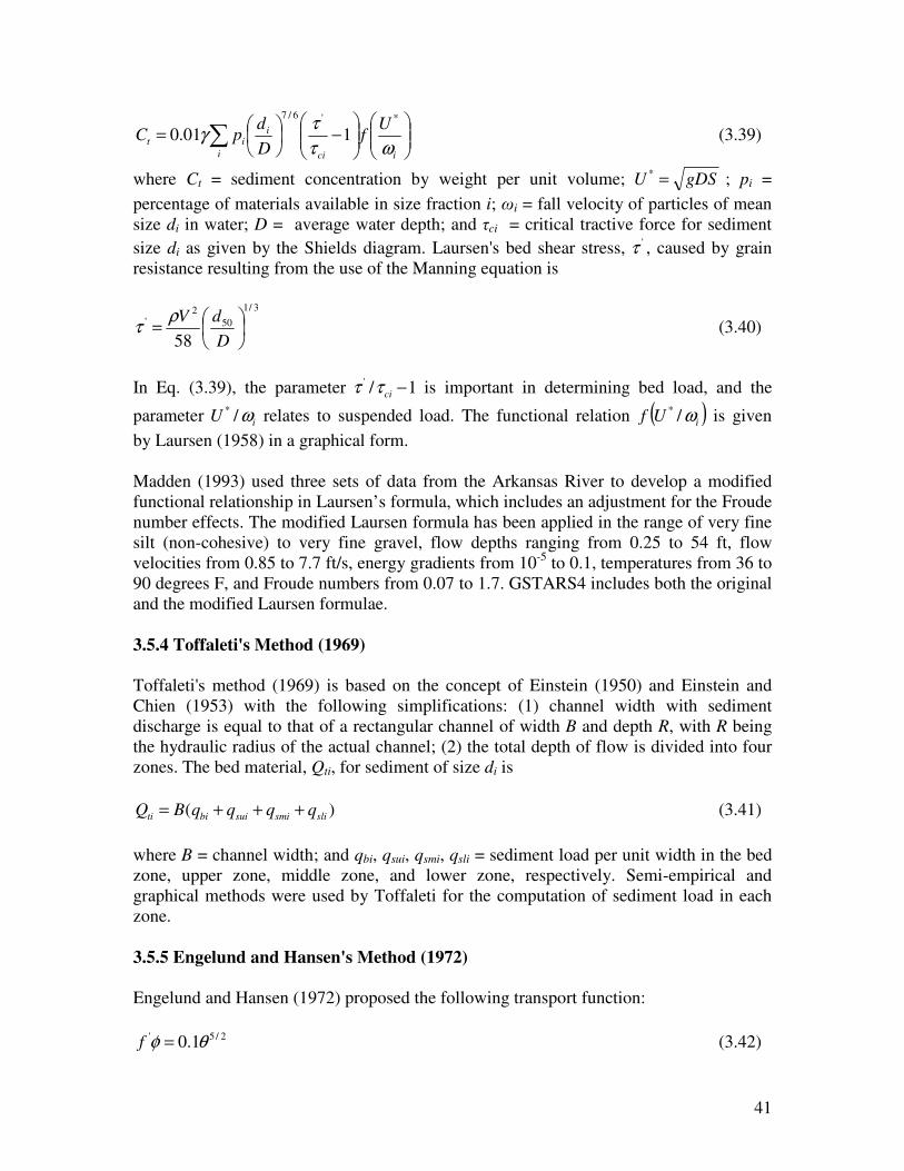
41
−
= ∑
ii ci
iit
Uf
D
dpC
ωτ
τγ
*'6/7
101.0 (3.39)
where Ct = sediment concentration by weight per unit volume; gDSU =* ; pi =
percentage of materials available in size fraction i; ωi = fall velocity of particles of mean
size di in water; D = average water depth; and τci = critical tractive force for sediment
size di as given by the Shields diagram. Laursen's bed shear stress, 'τ , caused by grain
resistance resulting from the use of the Manning equation is
3/1
50
2'
58
=
D
dVρτ (3.40)
In Eq. (3.39), the parameter 1/' −ciττ is important in determining bed load, and the
parameter iU ω/* relates to suspended load. The functional relation ( )iUf ω/* is given
by Laursen (1958) in a graphical form.
Madden (1993) used three sets of data from the Arkansas River to develop a modified
functional relationship in Laursen’s formula, which includes an adjustment for the Froude
number effects. The modified Laursen formula has been applied in the range of very fine
silt (non-cohesive) to very fine gravel, flow depths ranging from 0.25 to 54 ft, flow
velocities from 0.85 to 7.7 ft/s, energy gradients from 10-5
to 0.1, temperatures from 36 to
90 degrees F, and Froude numbers from 0.07 to 1.7. GSTARS4 includes both the original
and the modified Laursen formulae.
3.5.4 Toffaleti's Method (1969)
Toffaleti's method (1969) is based on the concept of Einstein (1950) and Einstein and
Chien (1953) with the following simplifications: (1) channel width with sediment
discharge is equal to that of a rectangular channel of width B and depth R, with R being
the hydraulic radius of the actual channel; (2) the total depth of flow is divided into four
zones. The bed material, Qti, for sediment of size di is
)( slismisuibiti qqqqBQ +++= (3.41)
where B = channel width; and qbi, qsui, qsmi, qsli = sediment load per unit width in the bed
zone, upper zone, middle zone, and lower zone, respectively. Semi-empirical and
graphical methods were used by Toffaleti for the computation of sediment load in each
zone.
3.5.5 Engelund and Hansen's Method (1972)
Engelund and Hansen (1972) proposed the following transport function:
2/5' 1.0 θφ =f (3.42)

42
2
' 2
V
gSDf = (3.43)
2/1
3
−
−= gd
q s
s
t
γ
γγ
γφ (3.44)
( )ds γγ
τθ
−= (3.45)
where g = gravitational acceleration; S = energy slope; V = average flow velocity; qt =
total sediment discharge by weight per unit width; γs and γ = specific weights of
sediment and water, respectively; d = median particle diameter; D = mean water depth;
and τ = shear stress along the bed.
3.5.6 Ackers and White's Method (1973) and (1990)
Ackers and White (1973) applied dimensional analysis to express the mobility and
transport rate of sediment in terms of some dimensionless parameters. Their mobility
number for sediment is
( )
n
sn
grdD
VgdUF
−−
−=
12/1
*
/log321
αγ
γ (3.46)
where U*= shear velocity; n = transition exponent, depending on sediment size; α = 10, in
turbulent flow; d = sediment particle size; and D = water depth. They also expressed the
sediment size by a dimensionless grain diameter:
3/1
21
−=
γ
γ
νs
gr
gdd (3.47)
where ν = kinematic viscosity of water. A dimensionless sediment transport function can
then be expressed as
( )grgrgr dFfG ,= (3.48)
with
( )
n
s
grV
U
d
XDG
=
*
/γγ (3.49)
where X = rate of sediment transport in terms of mass flow per unit mass flow rate, i.e.,
concentration by weight of fluid flux. The generalized dimensionless sediment transport
function can also be expressed as

43
m
gr
grA
FCG
−= 1 (3.50)
The values of A, C, m, and n were determined by Ackers and White (1973) based on best-
fit curves of laboratory data with sediment size greater than 0.04 mm and Froude number
less than 0.8.
The original Ackers and White formula is known to overpredict transport rates for fine
sediments (smaller than 0.2 mm) and for relatively coarse sediments. To correct that
tendency, a revised form of the coefficients was published in 1990 (HR Wallingford,
1990). Both versions of the coefficients are included in GSTARS4. The comparison
between the original and the revised coefficients is given in table 3.2.
Table 3.2 Coefficients for the 1973 and 1990 versions of the Ackers and White formula.
3.5.7 Yang's Sand (1973) and Gravel (1984) Transport Formulae
Yang's 1973 dimensionless unit stream power formula for sand transport is
−
−−+
−−=
ωωων
ω
ων
ω
SVVSUd
UdC
cr
ts
loglog314.0log409.0799.1
log457.0log286.0435.5log
*
*
(3.51)
where Cts = total sand concentration in parts per million by weight; ω = sediment fall
velocity; d = sediment particle diameter; ν = kinematic viscosity of water; U*= shear
velocity; VS = unit stream power; V = average flow velocity; S = water surface or energy
slope; and Vcr = critical average flow velocity at incipient motion. The coefficients in Eq.
(3.51) were determined from 463 sets of laboratory flume data. Eq. (3.51) should be
applied to sand transport with particle diameter less than 2 mm.

44
The critical dimensionless unit stream power, VcrS / ω, is the product of dimensionless
critical velocity Vcr / ω and energy slope S, where
=ω
crV ( ) 66.0
06.0/log
5.2*
+−νdU
if 1.2 ≤ ν
dU*
≤ 70 (3.52)
2.05 if 70 ≤ ν
dU*
Yang's 1984 dimensionless unit stream power formula for gravel transport with particle
diameter equal to or greater than 2 mm is
−
−−+
−−=
ωωων
ω
ων
ω
SVVSUd
UdC
cr
tg
loglog282.0log305.0784.2
log816.4log633.0681.6log
*
*
(3.53)
where Ctg = total gravel concentration in parts per million by weight. The coefficients in
Eq. (3.53) were determined from 167 sets of laboratory flume data.
The incipient motion criteria given in Eq. (3.52) should be used for Eqs. (3.51) and (3.53).
Because of the range of data used for the determination of the coefficients in Eq. (3.53),
the equation should be applied to gravel with median particle size between 2 and 10 mm.
However, published literature suggests that Eq. (3.53) may be applicable to materials
coarser than 10 mm. GSTARS4 uses Eq. (3.53) for sizes up to 100 mm. Eqs. (3.51) and
(3.53) were originally derived for uniform materials. When they are applied to
nonuniform materials, the total sediment concentration should be computed by using Eq.
(3.28).
For natural rivers, the bed-material size may vary from sand to gravel. In this case, the
use of both Eqs. (3.51) and (3.53) should be considered. GSTARS4 uses the appropriate
equation for a given particle size.
3.5.8 Yang's Sand (1979) and Gravel (1984) Transport Formulae
Yang (1979) proposed a sand transport formula for flow conditions well exceeding those
required for incipient motion. In this case, the dimensionless critical unit stream power
required at incipient motion can be neglected. Yang's 1979 sand transport formula for
sediment concentration greater than 100 parts per million by weight is

45
ωων
ω
ων
ω
VSUd
UdCts
loglog480.0log360.0780.1
log297.0log153.0165.5log
*
*
−−+
−−=
(3.54)
The coefficients in Eq. (3.54) were determined from 452 sets of laboratory flume data.
Eqs. (3.51) and (3.54) give about the same degree of accuracy when the bed-material
concentration is greater than about 100 parts per million by weight. Users can either use a
combination of Eqs. (3.51) and (3.53) or (3.54) and (3.53) for the computation of bed
material concentration in a river, depending on sediment size in that river. If bed
materials are not uniform, Eq. (3.28) is also applied in GSTARS4.
3.5.9 Parker's Method (1990)
Parker (1990) developed an empirical gravel transport function based on the equal
mobility concept and field data. Parker's dimensionless bed-load transport function, *
iW ,
and dimensionless shear stress parameter, iφ , are defined as
gDSDSp
qW
i
bisi
−= 1*
γ
γ (3.55)
1
*1
−
−=
γ
γ
τφ s
rii
id
DS (3.56)
The value of *
riτ based on d50 is 0.875, i.e.,
i
rid
d50* 875.0=τ (3.57)
where qbi = bed-load per unit channel width in size fraction di; D = water depth; S =
slope; and pi = fraction by weight in size di.
Because of equal mobility of all sizes, only one grain size, namely, the subpavement size,
d50, is used to characterize bed-load discharge as a function of the dimensionless shear
stress, i.e.,
=*W 2.14
500025.0 φ if 0.150 <φ
( ) ( ) 2
5050 128.912.14exp0025.0 −−− φφ if 59.10.1 50 ≤≤ φ (3.58)
5.4
50
853.01685.13
−
φ if 59.150 >φ
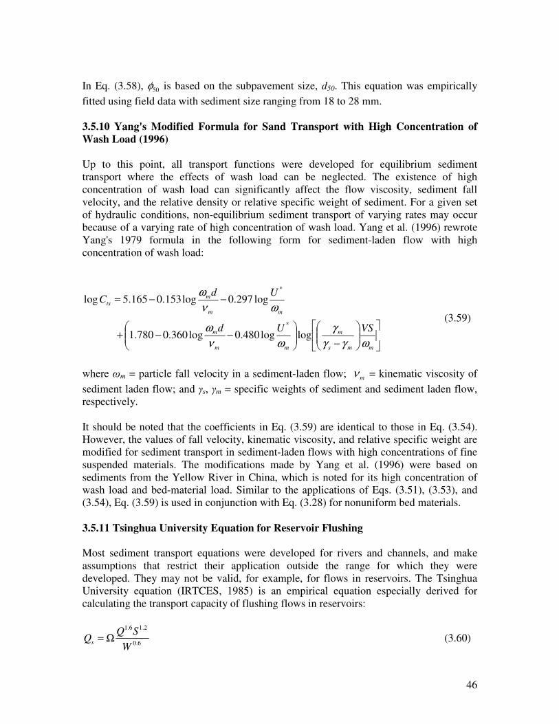
46
In Eq. (3.58), 50φ is based on the subpavement size, d50. This equation was empirically
fitted using field data with sediment size ranging from 18 to 28 mm.
3.5.10 Yang's Modified Formula for Sand Transport with High Concentration of
Wash Load (1996)
Up to this point, all transport functions were developed for equilibrium sediment
transport where the effects of wash load can be neglected. The existence of high
concentration of wash load can significantly affect the flow viscosity, sediment fall
velocity, and the relative density or relative specific weight of sediment. For a given set
of hydraulic conditions, non-equilibrium sediment transport of varying rates may occur
because of a varying rate of high concentration of wash load. Yang et al. (1996) rewrote
Yang's 1979 formula in the following form for sediment-laden flow with high
concentration of wash load:
−
−−+
−−=
mms
m
mm
m
mm
mts
VSUd
UdC
ωγγ
γ
ων
ω
ων
ω
loglog480.0log360.0780.1
log297.0log153.0165.5log
*
*
(3.59)
where ωm = particle fall velocity in a sediment-laden flow; mν = kinematic viscosity of
sediment laden flow; and γs, γm = specific weights of sediment and sediment laden flow,
respectively.
It should be noted that the coefficients in Eq. (3.59) are identical to those in Eq. (3.54).
However, the values of fall velocity, kinematic viscosity, and relative specific weight are
modified for sediment transport in sediment-laden flows with high concentrations of fine
suspended materials. The modifications made by Yang et al. (1996) were based on
sediments from the Yellow River in China, which is noted for its high concentration of
wash load and bed-material load. Similar to the applications of Eqs. (3.51), (3.53), and
(3.54), Eq. (3.59) is used in conjunction with Eq. (3.28) for nonuniform bed materials.
3.5.11 Tsinghua University Equation for Reservoir Flushing
Most sediment transport equations were developed for rivers and channels, and make
assumptions that restrict their application outside the range for which they were
developed. They may not be valid, for example, for flows in reservoirs. The Tsinghua
University equation (IRTCES, 1985) is an empirical equation especially derived for
calculating the transport capacity of flushing flows in reservoirs:
6.0
2.16.1
W
SQQs Ω= (3.60)
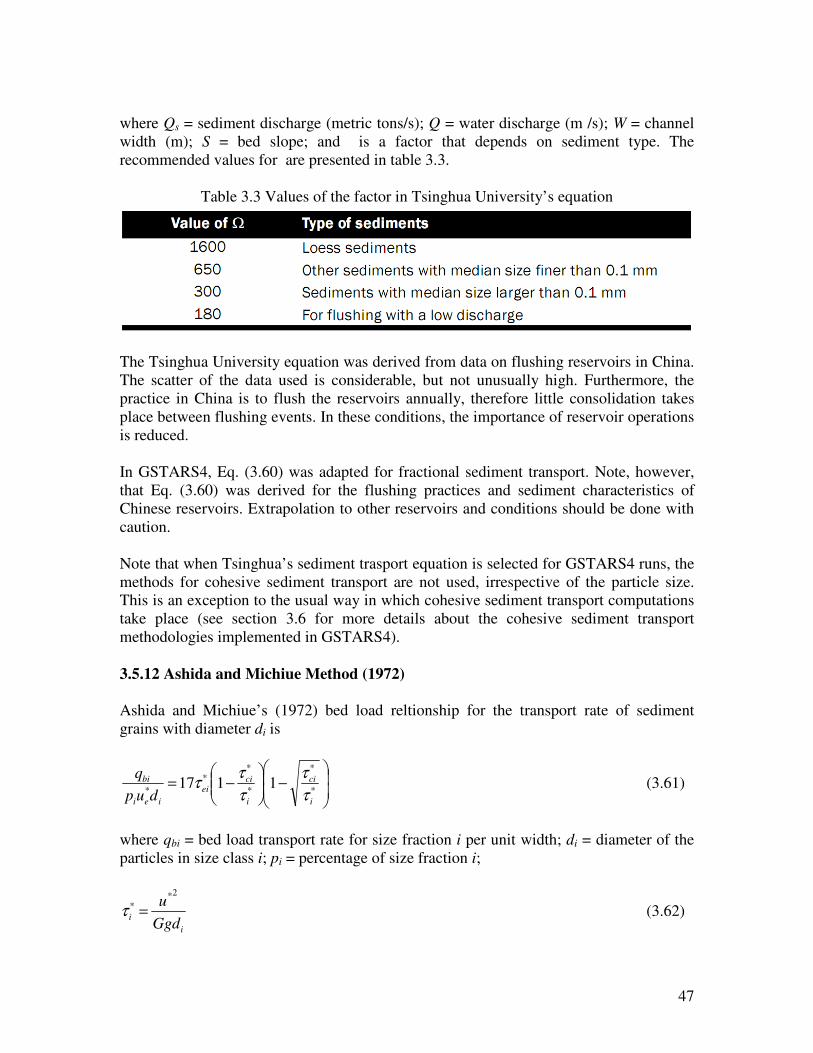
47
where Qs = sediment discharge (metric tons/s); Q = water discharge (m /s); W = channel
width (m); S = bed slope; and is a factor that depends on sediment type. The
recommended values for are presented in table 3.3.
Table 3.3 Values of the factor in Tsinghua University’s equation
The Tsinghua University equation was derived from data on flushing reservoirs in China.
The scatter of the data used is considerable, but not unusually high. Furthermore, the
practice in China is to flush the reservoirs annually, therefore little consolidation takes
place between flushing events. In these conditions, the importance of reservoir operations
is reduced.
In GSTARS4, Eq. (3.60) was adapted for fractional sediment transport. Note, however,
that Eq. (3.60) was derived for the flushing practices and sediment characteristics of
Chinese reservoirs. Extrapolation to other reservoirs and conditions should be done with
caution.
Note that when Tsinghua’s sediment trasport equation is selected for GSTARS4 runs, the
methods for cohesive sediment transport are not used, irrespective of the particle size.
This is an exception to the usual way in which cohesive sediment transport computations
take place (see section 3.6 for more details about the cohesive sediment transport
methodologies implemented in GSTARS4).
3.5.12 Ashida and Michiue Method (1972)
Ashida and Michiue’s (1972) bed load reltionship for the transport rate of sediment
grains with diameter di is
−
−=
*
*
*
**
*1117
i
ci
i
ciei
iei
bi
dup
q
τ
τ
τ
ττ (3.61)
where qbi = bed load transport rate for size fraction i per unit width; di = diameter of the
particles in size class i; pi = percentage of size fraction i;
i
iGgd
u2*
* =τ (3.62)
48
i
cici
Ggd
u2*
* =τ (3.63)
i
eei
Ggd
u2*
* =τ (3.64)
Where u* = shear velocity ( ehSgR ); G = specific gravity of sediments in water; g =
acceleration due to gravity; Rh = hydraulic radius; Se = slope of the energy line; *
eu =
effective shear velocity, computed
0.621
/log75.5
*
50
*+
+=
τ
dR
u
v h
e
(3.65)
where d50 = mean diameter of the bed material. The critical shear stress for each size
class is expressed following Egiazaroff (1965):
=2*
50
2
c
ci
u
u 85.0 if
50d
di < 0.4 (3.66)
2
50
19log
19log
d
di
if 50d
di ≥ 0.4
where *
50cu = nondimensional critical shear velocity for the d50 fraction:
50
*
50
*
50 Ggdu cc τ= (3.67)
*
50cτ is taken equal to 0.05.
Although the original expression due to Ashida and Michiue (1972) is for bed load only,
in GSTARS4 the method of Ashida and Mishiue (1970) is used to compute the suspended
load, therefore the implementation falls in the bed-material load category.
The transport rate per unit width of the suspended load, for size fraction i, is computed
following Ashida and Michiue (1970):
( )1
1
11
c
eeevCq
achcac
aisi
−− −= (3.68)
49
where Cai = concentration at a reference level (assumed to be a = 0.05h, where h is the
water depth), which is given by
( ) ( )
−= 0
0
0 ξξ
ξF
fKpC iai (3.69)
with
( ) 2
00 5.0exp2
1ξ
πξ −=f (3.70)
( ) ∫∞
−=0
2
0 5.0exp2
1
ξξξ
πξ dF (3.71)
where K = 0.025, ( )*
0 75.0/ uiωξ = , and ωi is the fall velocity of sediment particles with
diameter di. In Eq. (3.68), ci is computed as
huc i
i *
6
κ
ω= (3.72)
where κ is the von Kármán constant (= 0.412).
The total load per unit width for size fraction i is found by adding the bed load and the
suspended load obtained by Eqs. (3.61) and (3.68), respectively: qi = qbi + qsi. Ashida
and Michiue’s formulation has been widely used, with success, by Japanese engineers
and scientists working in river and reservoir sedimentation.
Due to the nature of Ashida and Michiue’s method, the parameter r in Eq. (3.28) should
be set to 1 when the method is used in GSTARS4 runs.
3.6 Cohesive Sediment Transport
At present, the equations for computing the transport potential of cohesive sediments†
implemented in GSTARS4 are considered state-of-the-art (Partheniades, 1986; Mehta et
al., 1989). However, in spite of the progress of recent years in modeling cohesive
sediment transport, reliable predictive techniques are still not available. In practice,
modeling of fines still relies on extensive calibration and sensitivity analysis, techniques
that are useful and can yield excellent results, but that are costly and time consuming.
† In this manual, cohesive sediments are sediments whose particles pass through a 62.5 µm sieve,
a definition that follows the nomenclature of the American Geophysical Union (Lane, 1947). We
also use the terms mud and fines to refer to this type of sediment. See table 3.4 for more detailed
description of the subclasses.
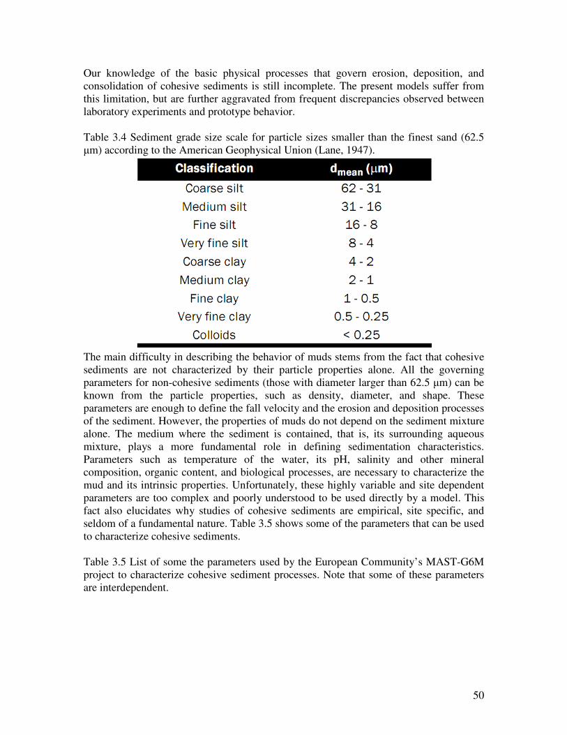
50
Our knowledge of the basic physical processes that govern erosion, deposition, and
consolidation of cohesive sediments is still incomplete. The present models suffer from
this limitation, but are further aggravated from frequent discrepancies observed between
laboratory experiments and prototype behavior.
Table 3.4 Sediment grade size scale for particle sizes smaller than the finest sand (62.5
µm) according to the American Geophysical Union (Lane, 1947).
The main difficulty in describing the behavior of muds stems from the fact that cohesive
sediments are not characterized by their particle properties alone. All the governing
parameters for non-cohesive sediments (those with diameter larger than 62.5 µm) can be
known from the particle properties, such as density, diameter, and shape. These
parameters are enough to define the fall velocity and the erosion and deposition processes
of the sediment. However, the properties of muds do not depend on the sediment mixture
alone. The medium where the sediment is contained, that is, its surrounding aqueous
mixture, plays a more fundamental role in defining sedimentation characteristics.
Parameters such as temperature of the water, its pH, salinity and other mineral
composition, organic content, and biological processes, are necessary to characterize the
mud and its intrinsic properties. Unfortunately, these highly variable and site dependent
parameters are too complex and poorly understood to be used directly by a model. This
fact also elucidates why studies of cohesive sediments are empirical, site specific, and
seldom of a fundamental nature. Table 3.5 shows some of the parameters that can be used
to characterize cohesive sediments.
Table 3.5 List of some the parameters used by the European Community’s MAST-G6M
project to characterize cohesive sediment processes. Note that some of these parameters
are interdependent.

51
In GSTARS4, the transport of silt and clay is computed separately from the remaining
size fractions. GSTARS4 recognizes the presence of clay if any of the particle size
fractions given in the input has a geometric mean grain size, dmean, smaller than 0.004 mm
(see table 3.4). Similarly, the presence of silt is recognized if a size faction has a dmean
between 0.004 and 0.0625 mm. There can be any number of particle groups in the clay or
silt sizes, up to a maximum of 10 combined groups (i.e., including cohesive and non-
cohesive sediment size groups). While the transport of fractions with dmean ≥ 0.0625 mm
is computed by the traditional transport equations presented in section 3.5, for smaller
fractions the methods described in this section are used.
3.6.1 Deposition
The occurrence of erosion or deposition is controlled by the value of the bed shear stress,
τb. Deposition of clay and silt takes place when τb is smaller than the critical bed shear
stress for deposition, τcd. τcd is the critical value of the bed shear stress above which no
deposition occurs. In this case, the deposition is governed by integrating

52
h
CP
dt
dC sω−= (3.73)
where C = depth-averaged concentration of sediments, h = the water depth, and ωs = the
settling velocity of the sediment. P is a parameter representing the probability for
deposition, and is computed from
=P cd
b
τ
τ−1 when cdb ττ < (3.74)
0 when cdb ττ ≥
When ωs does not depend on the concentration of suspended sediments (unhindered
settling), Eq. (3.73) can be integrated analytically to yield
−
∆−=
cd
bs
h
t
C
C
τ
τω1exp
0
(3.75)
where C0 and C are the concentration at the beginning and end of time step. The time of
residence, ∆t, is obtained from x/V, where ∆x is the reach length and V is the velocity of
the flow.
For higher concentrations of suspended sediments, ωs becomes dependent of
concentration via effects of flocculation and hindered settling (see figure 3.7). In those
cases, Eq. (3.73) does not offer a closed form solution. For high concentrations,
GSTARS4 integrates Eq. (3.73) numerically to obtain:
−
∆−=
cd
bs
h
tCCC
τ
τω10
0 (3.76)
in which ωs is computed from expressions discussed later, in section 3.8, and is assumed
to remain constant during the time step. Eqs. (3.75) and (3.76) are both included in
GSTARS4. The concentration obtained from their solution is converted into volume and
deposited on the bed.
It was mentioned that the adoption of Eq. (3.75) requires unhindered settling conditions
of the sediment particles. Unhindered settling is a condition under which the particles
retain their individuality, and only occurs at relatively low concentrations, say C < C1. At
higher concentrations, particles flocculate together, forming larger aggregates that behave
differently from the individual particles. Values of C1 are in the range of 100 to 700 mg/l.
At these values of the concentration, fall velocity increases due to the increased weight of
the aggregates. At even higher concentrations, say C > C2, the larger size of the
aggregates actually works to slow down their fall velocities, in a similar effect as that of a
parachute. Typical values of C2 are in the range of 5 to 10 g/l. However, these limits are
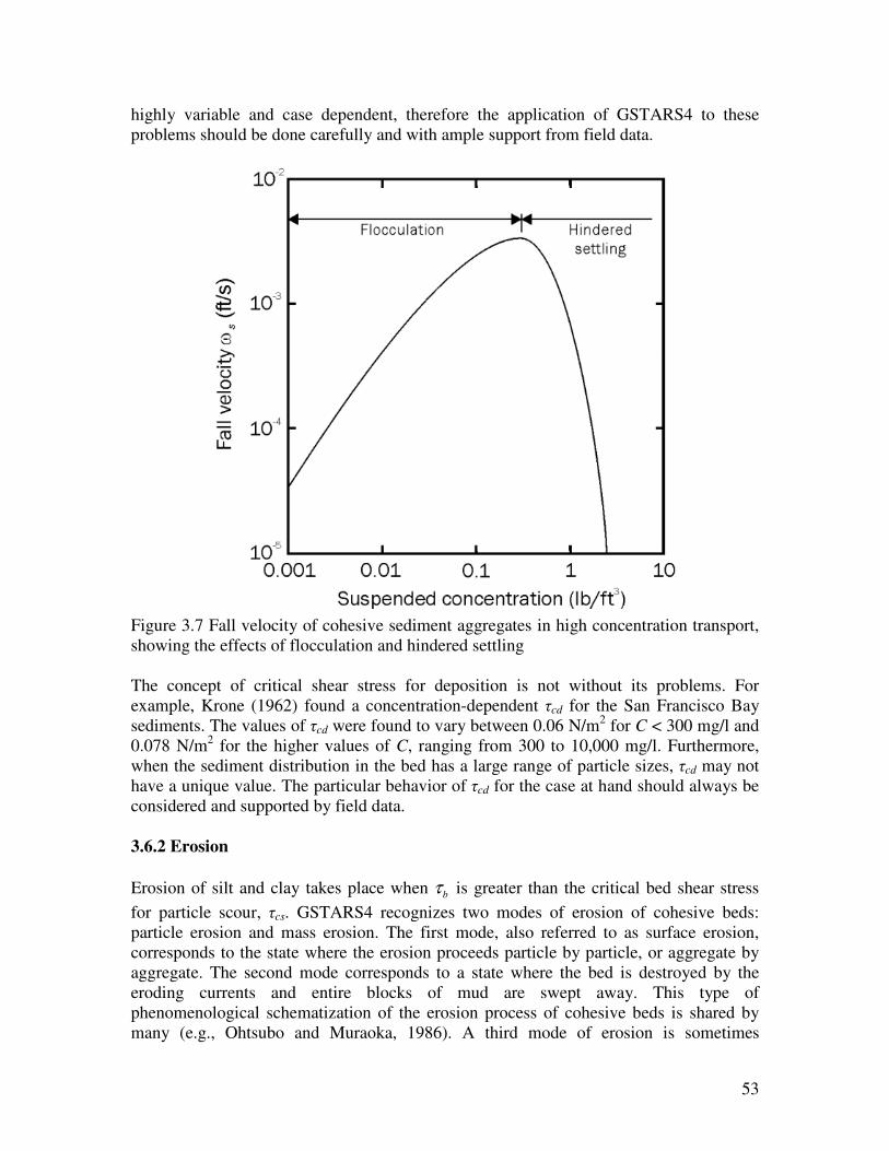
53
highly variable and case dependent, therefore the application of GSTARS4 to these
problems should be done carefully and with ample support from field data.
Figure 3.7 Fall velocity of cohesive sediment aggregates in high concentration transport,
showing the effects of flocculation and hindered settling
The concept of critical shear stress for deposition is not without its problems. For
example, Krone (1962) found a concentration-dependent τcd for the San Francisco Bay
sediments. The values of τcd were found to vary between 0.06 N/m2 for C < 300 mg/l and
0.078 N/m2 for the higher values of C, ranging from 300 to 10,000 mg/l. Furthermore,
when the sediment distribution in the bed has a large range of particle sizes, τcd may not
have a unique value. The particular behavior of τcd for the case at hand should always be
considered and supported by field data.
3.6.2 Erosion
Erosion of silt and clay takes place when bτ is greater than the critical bed shear stress
for particle scour, τcs. GSTARS4 recognizes two modes of erosion of cohesive beds:
particle erosion and mass erosion. The first mode, also referred to as surface erosion,
corresponds to the state where the erosion proceeds particle by particle, or aggregate by
aggregate. The second mode corresponds to a state where the bed is destroyed by the
eroding currents and entire blocks of mud are swept away. This type of
phenomenological schematization of the erosion process of cohesive beds is shared by
many (e.g., Ohtsubo and Muraoka, 1986). A third mode of erosion is sometimes

54
mentioned, which corresponds to the re-entrainment of a stationary suspension (Mehta et
al., 1989).
The current methods compute the rate of erosion, E‡, as a linear function of the excess of
the bed shear stress with respect to a critical shear stress for erosion:
−=
ci
cibiME
τ
ττ (3.77)
where i = 1,2 for particle or mass erosion, respectively, Mi is an experimental parameter,
and τci are the critical shear stresses for erosion. Mi and τci vary with type of sediment,
salinity and mineral contents of the water, its pH and temperature, but do not correlate
well with the parameters usually used to characterize noncohesive sediments (particle
diameter, specific gravity, Atterberg limits, etc. – see table 3.5). Therefore, to compute
the erosion rate of mud beds we need to know how M1, M2, τc1, and τc2 vary within the
domain of interest. This variation may be in space and/or time.
Unfortunately, the literature does not provide methods of estimating Mi, therefore Eq.
(3.77) was implemented in two stages. Particle erosion takes place when τb > τcs. Mass
erosion takes place when τb increases past the critical bed shear stress, τcm, for mass
erosion. The following equations are used for the particle and mass erosion rates,
respectively (Partheniades 1965; Ariathurai and Krone 1976):
cmbcs τττ ≤< :
−== 1
111
cs
bMdt
dm
AE
τ
τ (3.78)
cmb ττ > :
∆==
t
TM
dt
dm
AE e
22
1 (3.79)
where m = mass; t = time; ∆t = time step; M1, M2 = material constants that depend on
mineral composition, salinity, organic material, etc., with units of mass per unit area and
time; A = bottom area; and E1 = particle erosion rate per unit of area; E2 = mass erosion
rate per unit of area; and Te = characteristic time of erosion.
The presence of clay in the active layer may increase the cohesive forces between
particles. As a result, the shear stress necessary to move the cohesive materials may be
greater than that necessary to move the individual particles, which in turn limits the rates
of bed erosion. To model this effect, GSTARS4 uses an input parameter that indicates a
threshold value for the percentage of clay in the composition of the bed, above which the
erosion rates of silts, sands, and gravel are limited to the erosion rate of clay. For example,
if that parameter is set to 0.3 (i.e., 30 percent), whenever the composition of the bed
‡ Unit of mass of eroded sediment per unit of bed area and per unit of time.
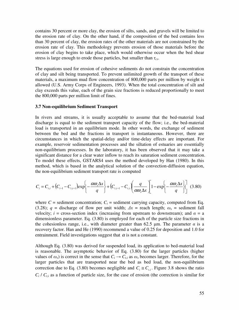
55
contains 30 percent or more clay, the erosion of silts, sands, and gravels will be limited to
the erosion rate of clay. On the other hand, if the composition of the bed contains less
than 30 percent of clay, the erosion rates of the other materials are not constrained by the
erosion rate of clay. This methodology prevents erosion of those materials before the
erosion of clay begins to take place, which would otherwise occur when the bed shear
stress is large enough to erode those particles, but smaller than τcs.
The equations used for erosion of cohesive sediments do not constrain the concentration
of clay and silt being transported. To prevent unlimited growth of the transport of these
materials, a maximum mud flow concentration of 800,000 parts per million by weight is
allowed (U.S. Army Corps of Engineers, 1993). When the total concentration of silt and
clay exceeds this value, each of the grain size fractions is reduced proportionally to meet
the 800,000 parts per million limit of fines.
3.7 Non-equilibrium Sediment Transport
In rivers and streams, it is usually acceptable to assume that the bed-material load
discharge is equal to the sediment transport capacity of the flow; i.e., the bed-material
load is transported in an equilibrium mode. In other words, the exchange of sediment
between the bed and the fractions in transport is instantaneous. However, there are
circumstances in which the spatial-delay and/or time-delay effects are important. For
example, reservoir sedimentation processes and the siltation of estuaries are essentially
non-equilibrium processes. In the laboratory, it has been observed that it may take a
significant distance for a clear water inflow to reach its saturation sediment concentration.
To model these effects, GSTARS4 uses the method developed by Han (1980). In this
method, which is based in the analytical solution of the convection-diffusion equation,
the non-equilibrium sediment transport rate is computed
( ) ( )
∆−−
∆−+
∆−−+= −−−
q
x
x
qCC
q
xCCCC s
s
itits
itiiti
αω
αω
αωexp1exp ,1,1,1, (3.80)
where C = sediment concentration; Ct = sediment carrying capacity, computed from Eq.
(3.28); q = discharge of flow per unit width; ∆x = reach length; ωs = sediment fall
velocity; i = cross-section index (increasing from upstream to downstream); and α = a
dimensionless parameter. Eq. (3.80) is employed for each of the particle size fractions in
the cohesionless range, i.e., with diameter greater than 62.5 µm. The parameter α is a
recovery factor. Han and He (1990) recommend a value of 0.25 for deposition and 1.0 for
entrainment. Field investigations suggest that α is not a constant.
Although Eq. (3.80) was derived for suspended load, its application to bed-material load
is reasonable. The asymptotic behavior of Eq. (3.80) for the larger particles (higher
values of ωs) is correct in the sense that Ci → Ct,i as ωs becomes larger. Therefore, for the
larger particles that are transported near the bed as bed load, the non-equilibrium
correction due to Eq. (3.80) becomes negligible and iti CC ,≅ . Figure 3.8 shows the ratio
Ci / Ct,i as a function of particle size, for the case of erosion (the correction is similar for
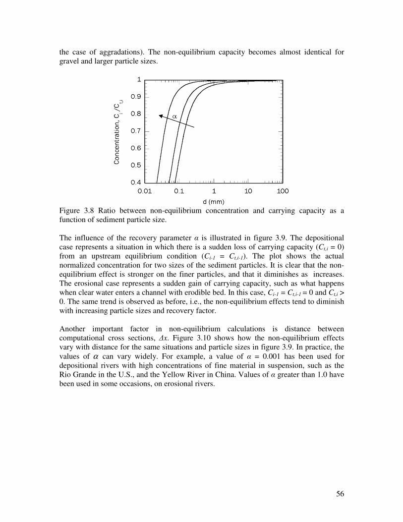
56
the case of aggradations). The non-equilibrium capacity becomes almost identical for
gravel and larger particle sizes.
Figure 3.8 Ratio between non-equilibrium concentration and carrying capacity as a
function of sediment particle size.
The influence of the recovery parameter α is illustrated in figure 3.9. The depositional
case represents a situation in which there is a sudden loss of carrying capacity (Ct,i = 0)
from an upstream equilibrium condition (Ci-1 = Ct,i-1). The plot shows the actual
normalized concentration for two sizes of the sediment particles. It is clear that the non-
equilibrium effect is stronger on the finer particles, and that it diminishes as increases.
The erosional case represents a sudden gain of carrying capacity, such as what happens
when clear water enters a channel with erodible bed. In this case, Ci-1 = Ct,i-1 = 0 and Ct,i >
0. The same trend is observed as before, i.e., the non-equilibrium effects tend to diminish
with increasing particle sizes and recovery factor.
Another important factor in non-equilibrium calculations is distance between
computational cross sections, ∆x. Figure 3.10 shows how the non-equilibrium effects
vary with distance for the same situations and particle sizes in figure 3.9. In practice, the
values of α can vary widely. For example, a value of α = 0.001 has been used for
depositional rivers with high concentrations of fine material in suspension, such as the
Rio Grande in the U.S., and the Yellow River in China. Values of α greater than 1.0 have
been used in some occasions, on erosional rivers.
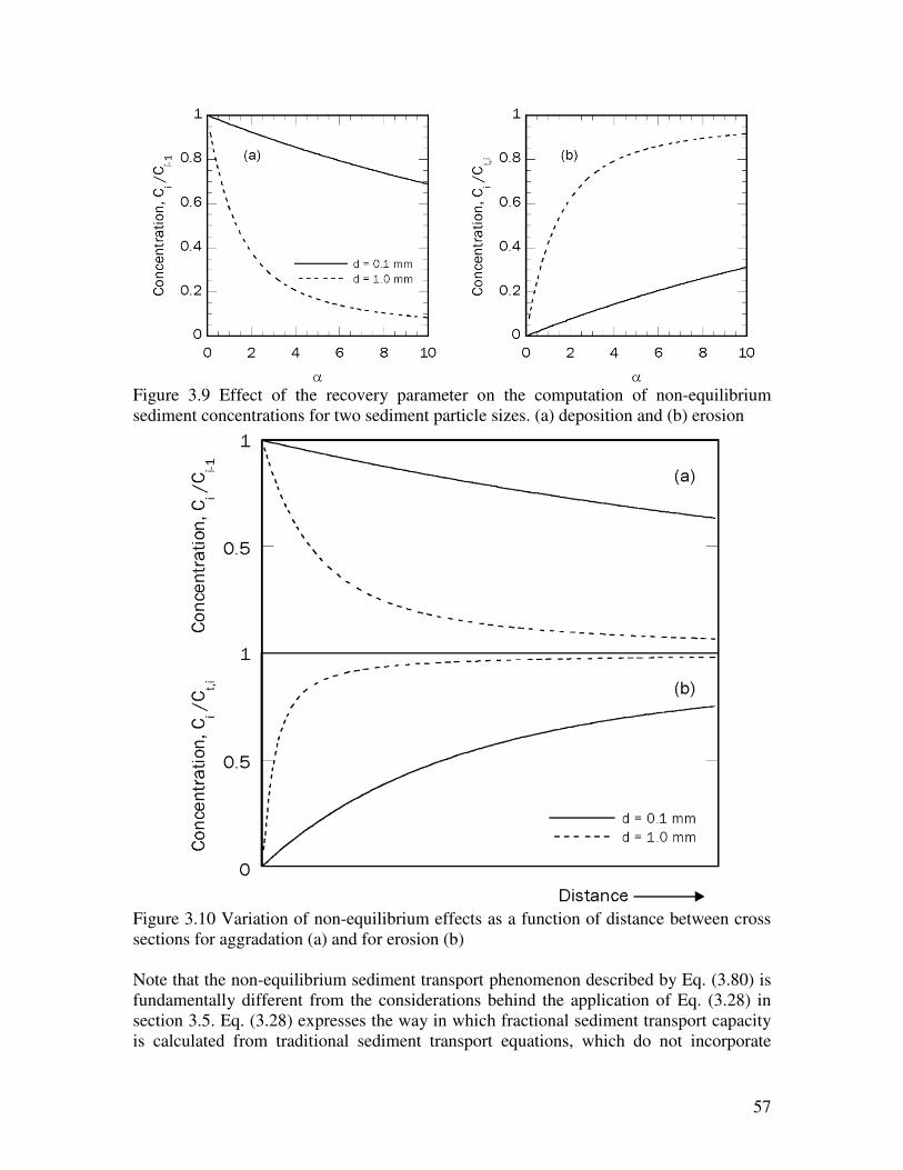
57
Figure 3.9 Effect of the recovery parameter on the computation of non-equilibrium
sediment concentrations for two sediment particle sizes. (a) deposition and (b) erosion
Figure 3.10 Variation of non-equilibrium effects as a function of distance between cross
sections for aggradation (a) and for erosion (b)
Note that the non-equilibrium sediment transport phenomenon described by Eq. (3.80) is
fundamentally different from the considerations behind the application of Eq. (3.28) in
section 3.5. Eq. (3.28) expresses the way in which fractional sediment transport capacity
is calculated from traditional sediment transport equations, which do not incorporate
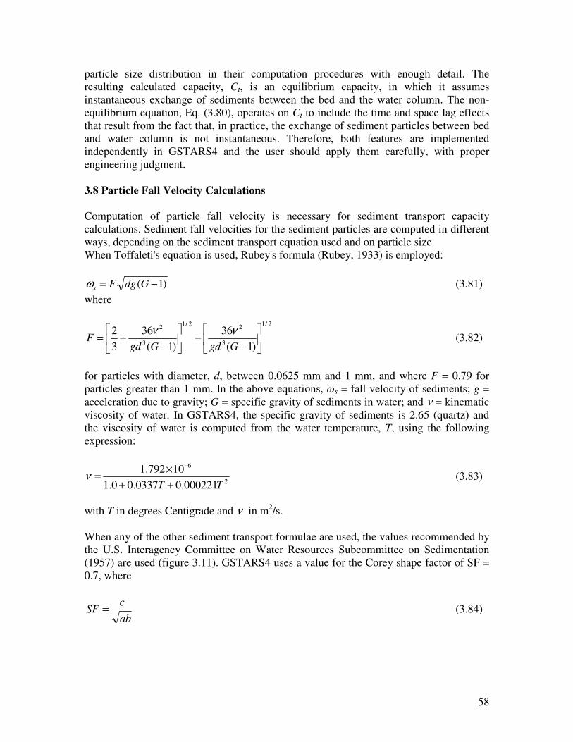
58
particle size distribution in their computation procedures with enough detail. The
resulting calculated capacity, Ct, is an equilibrium capacity, in which it assumes
instantaneous exchange of sediments between the bed and the water column. The non-
equilibrium equation, Eq. (3.80), operates on Ct to include the time and space lag effects
that result from the fact that, in practice, the exchange of sediment particles between bed
and water column is not instantaneous. Therefore, both features are implemented
independently in GSTARS4 and the user should apply them carefully, with proper
engineering judgment.
3.8 Particle Fall Velocity Calculations
Computation of particle fall velocity is necessary for sediment transport capacity
calculations. Sediment fall velocities for the sediment particles are computed in different
ways, depending on the sediment transport equation used and on particle size.
When Toffaleti's equation is used, Rubey's formula (Rubey, 1933) is employed:
)1( −= GdgFsω (3.81)
where
2/1
3
22/1
3
2
)1(
36
)1(
36
3
2
−−
−+=
GgdGgdF
νν (3.82)
for particles with diameter, d, between 0.0625 mm and 1 mm, and where F = 0.79 for
particles greater than 1 mm. In the above equations, ωs = fall velocity of sediments; g =
acceleration due to gravity; G = specific gravity of sediments in water; and ν = kinematic
viscosity of water. In GSTARS4, the specific gravity of sediments is 2.65 (quartz) and
the viscosity of water is computed from the water temperature, T, using the following
expression:
2
6
000221.00337.00.1
10792.1
TT ++
×=
−
ν (3.83)
with T in degrees Centigrade and ν in m2/s.
When any of the other sediment transport formulae are used, the values recommended by
the U.S. Interagency Committee on Water Resources Subcommittee on Sedimentation
(1957) are used (figure 3.11). GSTARS4 uses a value for the Corey shape factor of SF =
0.7, where
ab
cSF = (3.84)

59
where a, b, and c = the length of the longest, the intermediate, and the shortest mutually
perpendicular axes of the particle, respectively. For particles with diameter greater than
10 mm, which are above the range given in figure 3.11, the following formula is used:
gdGs )1(1.1 −=ω (3.85)
Figure 3.11 Relation between particle sieve diameter and its fall velocity according to the
U.S. Interagency Committee on Water Resources Subcommittee on Sedimentation (1957)
For particles in the silt and clay size ranges, that is, with diameters between 1 and 62.5
µm, the sediment fall velocities are computed from the following equations:
unhindered settling:
νω
18
)1( 2gdG
s
−= for 1CC < (3.86)
flocculation range:
N
s MC=ω for 21 CCC ≤≤ (3.87)
hindered settling:
l
s kC)1(0 −= ωω for 2CC > (3.88)
where ω0 is found by equating eqs.(3.87) and (3.88) at C = C2, i.e.,
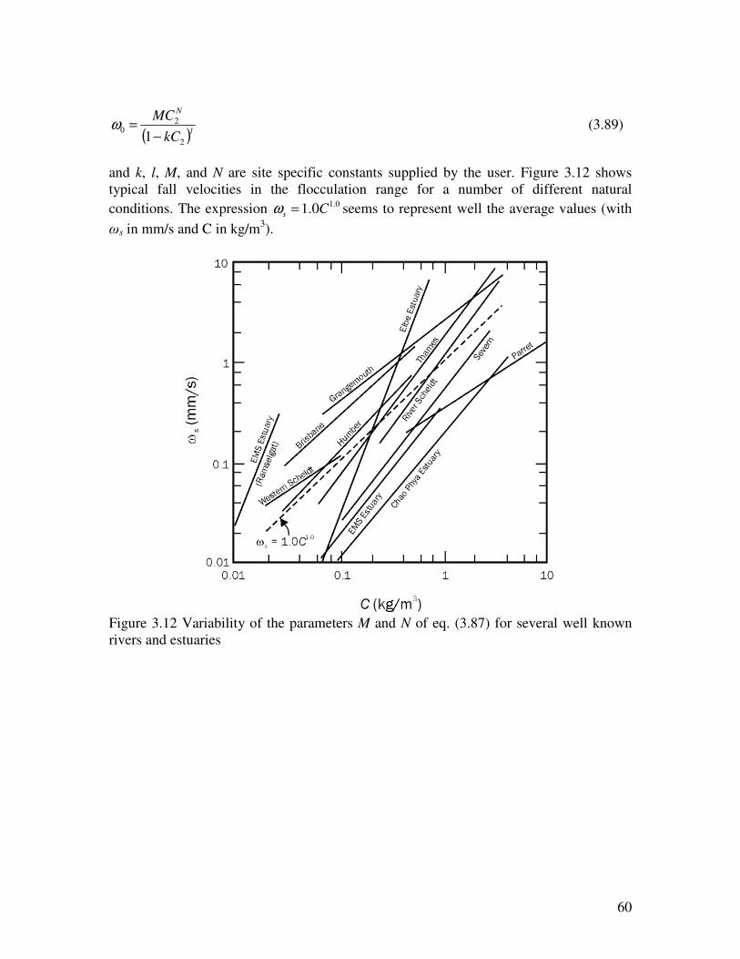
60
( )l
N
kC
MC
2
20
1−=ω (3.89)
and k, l, M, and N are site specific constants supplied by the user. Figure 3.12 shows
typical fall velocities in the flocculation range for a number of different natural
conditions. The expression 0.10.1 Cs =ω seems to represent well the average values (with
ωs in mm/s and C in kg/m3).
Figure 3.12 Variability of the parameters M and N of eq. (3.87) for several well known
rivers and estuaries
61
CHAPTER
4
COMPUTATION OF WIDTH CHANGES
GSTARS4 is able to compute not only channel bed elevation changes, but also channel
width changes. This chapter briefly describes the theoretical basis for those calculations
and their implementation in the numerical model. Note that this subject is very complex
and that its detailed presentation is not in the scope of this manual. The interested reader
is strongly encouraged to use the references in the chapter for a more rigorous and
complete presentation of the theory.
4.1 Theoretical Basis
Most one-dimensional models treat channel width as a constant value that does not
change with changing flow and sediment conditions. These models use the water depth,
D, the flow velocity, V, and channel slope, S, as independent variables. The three
independent equations that must be satisfied are the conservation of water,
Q = BDV (4.1)
where Q = water discharge and B = channel width; a flow resistance equation (Chézy's
equation is used for convenience),
2/1
= S
P
BDCV (4.2)
62
where C = roughness coefficient and P = wetted perimeter; and a sediment trans-
port equation,
( ),...,,,, dSVBDfQs = (4.3)
where Qs = sediment transport capacity and d = sediment particle size. However, a fourth
independent relationship must be used if the channel width is to be considered as another
independent variable. In GSTARS4, the theory of total stream power minimization is
used as a starting point to obtain the additional independent equation.
The basic theory behind the determination of width and depth adjustments is based on the
minimum energy dissipation rate theory developed by Song and Yang (1979a; 1979b;
1982a; 1982b) and Yang and Song (1979; 1986) and this general theory's special case,
the minimum stream power theory, used by Chang and Hill (1976; 1977; 1982) and
Chang (1979; 1980a; 1980b; 1982a; 1982b; 1983). The minimum energy dissipation rate
theory (Yang and Song, 1986) states that when a closed and dissipative system reaches its
state of dynamic equilibrium, its energy dissipation rate must be at its minimum value:
SW Φ+Φ=Φ = a minimum (4.4)
where Φ, ΦW, and ΦS are the total rate of energy dissipation, the rate of energy dissipation
due to water movement, and the rate of energy dissipation due to sediment movement,
respectively. The minimum value must be consistent with the constraints applied to the
system. If the system is not at its dynamic equilibrium condition, its energy dissipation
rate is not at its minimum value, but the system will adjust itself in a manner that will
reduce its energy dissipation rate to a minimum value and regain equilibrium. Because of
changing flow and sediment conditions, a natural river is seldom in its true equilibrium
condition. However, a natural river will adjust its channel geometry, slope, pattern,
roughness, etc., to minimize its energy dissipation rate subject to the water discharge and
sediment load supplied from upstream.
For an alluvial channel or river where the energy dissipation rate for transporting water is
much higher than that required to transport sediment, i.e., SW Φ>>Φ , the theory of
minimum energy dissipation rate can be replaced by a simplified theory of minimum
stream power (Yang, 1992). For this case, a river will minimize its stream power, γQS,
per unit channel length subject to hydrologic, hydraulic, sediment, geometric, geologic,
and man-made constraints. In the following equations, γ is the specific weight of water.
4.2 Computational Procedures
In order to apply the minimization procedure to channel reaches with gradually varied
flows, γQS is integrated along the channel:
∫=Φ QSdxT γ (4.5)
63
where ΦT is defined as the total stream power. This expression is discretized following
Chang (1982a):
( ) i
N
i
iiiiT xSQSQ ∆+=Φ ∑=
++1
112
1γ (4.6)
where N = number of stations along the reach; ∆x = reach length, or distance between
stations i and i+1; and Qi, Si = discharge and slope at station i, respectively. Choosing the
direction for channel adjustments is made by minimizing the integral represented by Eq.
(4.6) for total stream power at different stations. This process is repeated for each time
step: if alteration of the channel widths results in lower total stream power than raising or
lowering of the channel's bed, then channel adjustments progress in the lateral direction;
otherwise, the adjustments are made in the vertical direction.
Figure 4.1 is used to illustrate the process described above. When erosion takes place,
channel adjustments can proceed either by deepening or by widening the cross section.
Both channel widening and deepening can reduce the total stream power for the reach,
but GSTARS4 selects the adjustment that results in the minimum total stream power for
the reach. If deposition is predicted by the sediment routing computations, then either the
bed is raised or the cross section is narrowed, but the choice must also result in a
minimum of the total stream power for the reach. However, in each case the amount of
scour and/or deposition is limited by the predicted sediment load, and geological or man-
made restrictions are also accommodated by the computational algorithms.
Quantitatively, the amount of channel adjustment during each time step is determined by
the sediment continuity equation, i.e., Eq. (3.17) for each stream tube. Channel widening
or narrowing can take place only at the stream tubes adjacent to the banks. In this case,
the hydraulic radius, R, replaces the wetted perimeter, P, in Eq. (3.17). For stream tubes
that are not adjacent to the banks, i.e., interior tubes, bed adjustments can be made only in
the vertical direction. The process is briefly schematized in figure 4.2.
In summary, GSTARS4 channel geometry adjustments can occur in the vertical or lateral
directions, or in a combination of both. Whether the adjustment will proceed in the
vertical or lateral direction at a given time step of computation depends on which
direction results in less total stream power in accordance with the theory of minimum
total stream power. The requirement of reducing the total stream power during the
channel development process constitutes the basis for determining width or depth
adjustments in GSTARS4.
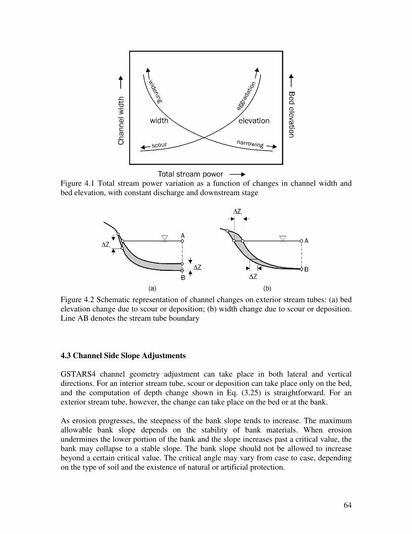
64
Figure 4.1 Total stream power variation as a function of changes in channel width and
bed elevation, with constant discharge and downstream stage
Figure 4.2 Schematic representation of channel changes on exterior stream tubes: (a) bed
elevation change due to scour or deposition; (b) width change due to scour or deposition.
Line AB denotes the stream tube boundary
4.3 Channel Side Slope Adjustments
GSTARS4 channel geometry adjustment can take place in both lateral and vertical
directions. For an interior stream tube, scour or deposition can take place only on the bed,
and the computation of depth change shown in Eq. (3.25) is straightforward. For an
exterior stream tube, however, the change can take place on the bed or at the bank.
As erosion progresses, the steepness of the bank slope tends to increase. The maximum
allowable bank slope depends on the stability of bank materials. When erosion
undermines the lower portion of the bank and the slope increases past a critical value, the
bank may collapse to a stable slope. The bank slope should not be allowed to increase
beyond a certain critical value. The critical angle may vary from case to case, depending
on the type of soil and the existence of natural or artificial protection.

65
GSTARS4 offers the user the option of checking the angle of repose for violation of a
known critical slope. If this option is chosen, the user must then supply the critical angle.
The user is also allowed the option of specifying one critical angle above the water
surface, and a different critical angle for submerged points. GSTARS4 scans each cross
section at the end of each time step to determine if any vertical or horizontal adjustments
have caused the banks to become too steep. If any violations occur, the two points
adjacent to the segment are adjusted vertically until the slope equals the user-provided
critical slope. For the situation shown in figure 4.3, the bank is adjusted from abde to
ab’d’e, so that the calculated angle, θ, is reduced to become equal to the critical angle, θc.
The adjustments are governed by conservation of mass:
A1 + A2 = A3 + A4 (4.7)
where A1 = area of triangle abb’a; A2 = area of triangle bcb’b; A3 = area of triangle cd’dc;
and A4 = area of triangle d’edd’.
Figure 4.3 Example of angle of repose adjustment

66
CHAPTER
5
RESERVOIR ROUTING
In GSTARS4, special treatments were developed to make the model better suited for
modeling flow and sediment transport in lakes, reservoirs, and water impoundments in
general. This was necessary because, although flow and sediment transport in lakes and
reservoirs are governed by the same physical laws as in rivers and channels, the
simplifications and approximations made in earlier versions of the model were mostly
based on observations made in riverine situations. Therefore, some modifications and
additions had to be made in order to extend and improve the model’s ability to handle
those cases. GSTARS3 is applicable for steady or quasi-steady flow simulation.
GSTARS4 is applicable to steady and unsteady flows.
There are many different types of water impoundments, and no model exists that can
successfully and indiscriminately be used for all. GSTARS4 is a semi-two-dimensional
model, therefore it may not be applicable to situations where fully two- or three-
dimensional models are required. GSTARS4 is best for run-of-the-river type of reservoirs,
and is particularly suited for long term simulations of large reservoirs, where limitations
in data availability, computational resources, time, or financial constraints preclude the
use of more sophisticated, multi-dimensional models.
5.1 Reservoir Routing
Sediment routing is accomplished by the same method described in section 2.1 (i.e., the
standard step method), but with some modifications. Within the reservoir subreach, the
water discharge is computed from a weighted averaged value using the river inflow and

67
the reservoir outflow discharges. The weighting parameter for each cross section is the
reservoir’s surface area represented by that cross section. For example, for the case
pictured in figure 5.1, the reservoir subreach starts in cross section 4 (the reservoir
subreach is defined by the cross sections whose thalweg is lower than the reservoir
elevation, Hres), therefore Q3 = Qin, where Qi = discharge at cross section i. The discharge
Q4 is given by
( )outinin QQaQQ −−= 44 (5.1)
where resAAa /44 = ; A4 = reservoir’s surface are represented by cross section 4; and Ares
= total surface area of the reservoir. In general,
( )∑=
−−=j
ik
koutininj aQQQQ (5.2)
where reskk AAa /= ; Ak = surface area of the reservoir represented by cross section k; i =
first cross section belonging to the reservoir subreach ( i = 4 in the example of figure 5.1).
of course that, from the definition of ak,
1=∑=
N
ik
ka (5.3)
where N = cross section at the dam (N = 8 in figure 5.1)

68
Figure 5.1 Subdivision of a GSTARS4 reach into river and reservoir subreaches for
reservoir routing. Top: side view; bottom: top view of the same reservoir. The shaded
region depicts the surface area of the reservoir represented by cross section #6
Water levels at the dam are calculated using level-pool routing. Assuming that the
reservoir water surface is horizontal,
t
VQQ outin
∆
∆=− (5.4)
where ∆V = change in the volume of water in the reservoir during time step ∆t. The
variation of storage is then used to determine the water level of the reservoir at the dam,
Hres, using a capacity table. The capacity table is a look-up table that is generated
incrementally as pictured in figure 5.2, in a similar fashion to Lewis (1996).
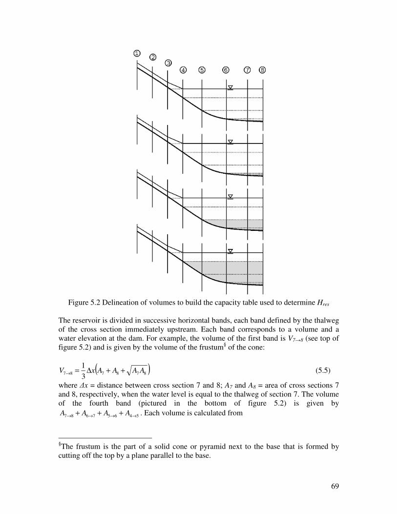
69
Figure 5.2 Delineation of volumes to build the capacity table used to determine Hres
The reservoir is divided in successive horizontal bands, each band defined by the thalweg
of the cross section immediately upstream. Each band corresponds to a volume and a
water elevation at the dam. For example, the volume of the first band is V7→8 (see top of
figure 5.2) and is given by the volume of the frustum§ of the cone:
( )8787873
1AAAAxV ++∆=→ (5.5)
where ∆x = distance between cross section 7 and 8; A7 and A8 = area of cross sections 7
and 8, respectively, when the water level is equal to the thalweg of section 7. The volume
of the fourth band (pictured in the bottom of figure 5.2) is given by
54657687 →→→→ +++ AAAA . Each volume is calculated from
§The frustum is the part of a solid cone or pyramid next to the base that is formed by
cutting off the top by a plane parallel to the base.
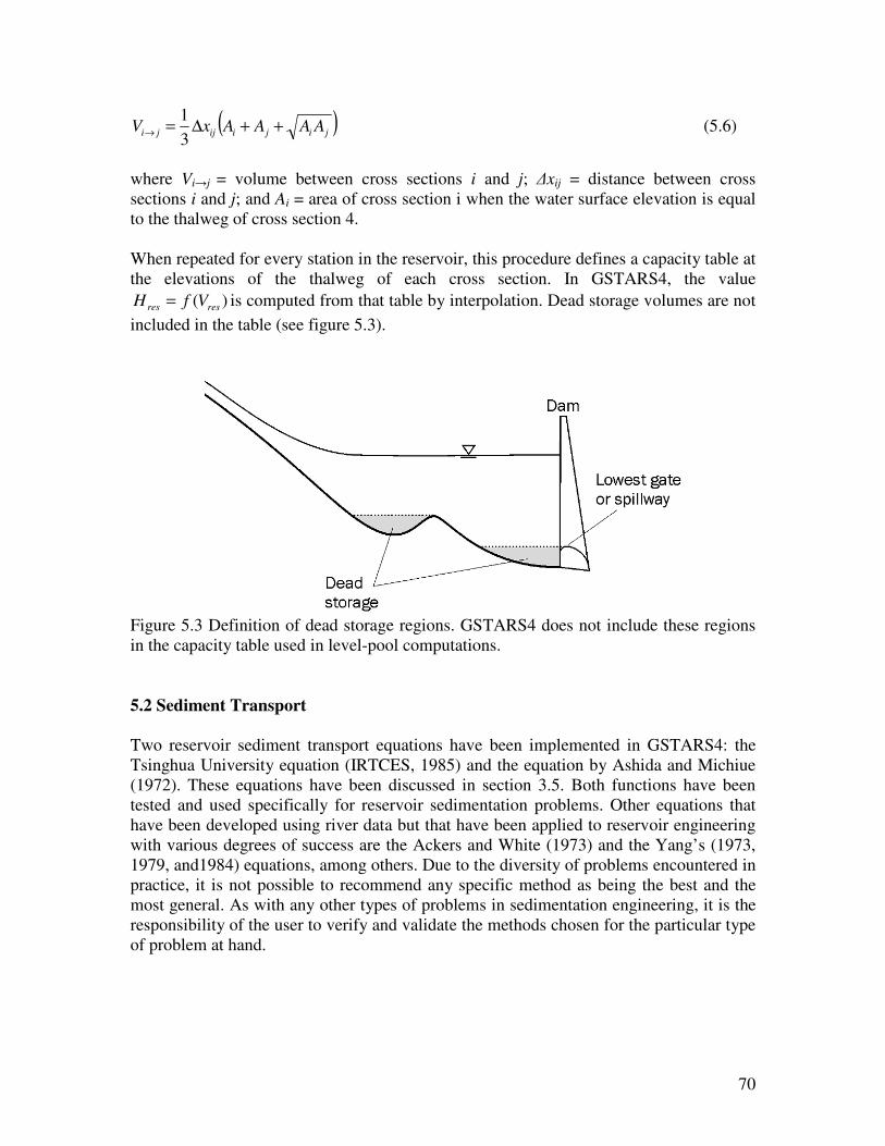
70
( )jijiijji AAAAxV ++∆=→3
1 (5.6)
where Vi→j = volume between cross sections i and j; ∆xij = distance between cross
sections i and j; and Ai = area of cross section i when the water surface elevation is equal
to the thalweg of cross section 4.
When repeated for every station in the reservoir, this procedure defines a capacity table at
the elevations of the thalweg of each cross section. In GSTARS4, the value
)( resres VfH = is computed from that table by interpolation. Dead storage volumes are not
included in the table (see figure 5.3).
Figure 5.3 Definition of dead storage regions. GSTARS4 does not include these regions
in the capacity table used in level-pool computations.
5.2 Sediment Transport
Two reservoir sediment transport equations have been implemented in GSTARS4: the
Tsinghua University equation (IRTCES, 1985) and the equation by Ashida and Michiue
(1972). These equations have been discussed in section 3.5. Both functions have been
tested and used specifically for reservoir sedimentation problems. Other equations that
have been developed using river data but that have been applied to reservoir engineering
with various degrees of success are the Ackers and White (1973) and the Yang’s (1973,
1979, and1984) equations, among others. Due to the diversity of problems encountered in
practice, it is not possible to recommend any specific method as being the best and the
most general. As with any other types of problems in sedimentation engineering, it is the
responsibility of the user to verify and validate the methods chosen for the particular type
of problem at hand.

71
The default technique used to compute bed changes has been described in section 3.3. It
consists in computing the bed elevation change ∆Z and applying it uniformly to all the
cross-sectional nodes in the wetted perimeter, resulting in a bed change that resembles
that in figure 3.3. However, in cases where deposition dominates and the rates of bed
change are slow (i.e., slow deposition), such as in many lakes and reservoirs, deposits are
formed by filling the lowest part of the channel first, producing flat cross section profiles,
as pictured in figure 5.4. In GSTARS4 the process is called “reservoir deposition”. In this
case, the cross-sectional area change, ∆Ad, is computed from ∆Z which is computed from
Eq. (3.18) using
ZWAd ∆=∆ (5.7)
where W is the cross section top width in the case of one stream tube, or the stream tube
top width in the case of computations using multiple stream tubes.
Figure 5.4 Reservoir deposition for a cross section. Compare to figure 3.3

72
CHAPTER
6
DATA REQUIREMENTS
Application of the GSTARS4 computer model requires the use of appropriate data. From
a conceptual point of view, GSTARS4 provides the governing equations and their
solution, and the user’s data provides geometric and hydrologic boundary information.
Together, data and computer program are what is called a model, in the sense that they
represent an approximation to a concrete and very specific physical reality. The degree of
approximation depends both on the physical and numerical representation implemented
in the computer program, and on the accuracy and completeness of the data.
The data requirements of GSTARS4 are described in this chapter. The data has to be
processed into ASCII data files that the computer program can understand. A plain ASCII
text editor should be used to type in the data in a specific format (as it was done for
earlier version of the GSTARS programs). In this chapter it is shown how to set-up that
data in an ASCII file that can be used to run the model from a DOS command line
window. The reader should go over this chapter carefully before using the GSTARS4
computer program.
6.1 Input Data Format
In GSTARS4 the data is organized in the same way as it was in previous versions of the
GSTARS models. Data is tabulated in ASCII files. The file is organized in sequential
records. A record is a line of up to 80 characters in length that is divided into fields of
fixed width (see figure 6.1). Fields are numbered from left to right, starting in the left-
most character. Field 0 is 2 characters long and is used to specify the record name (all
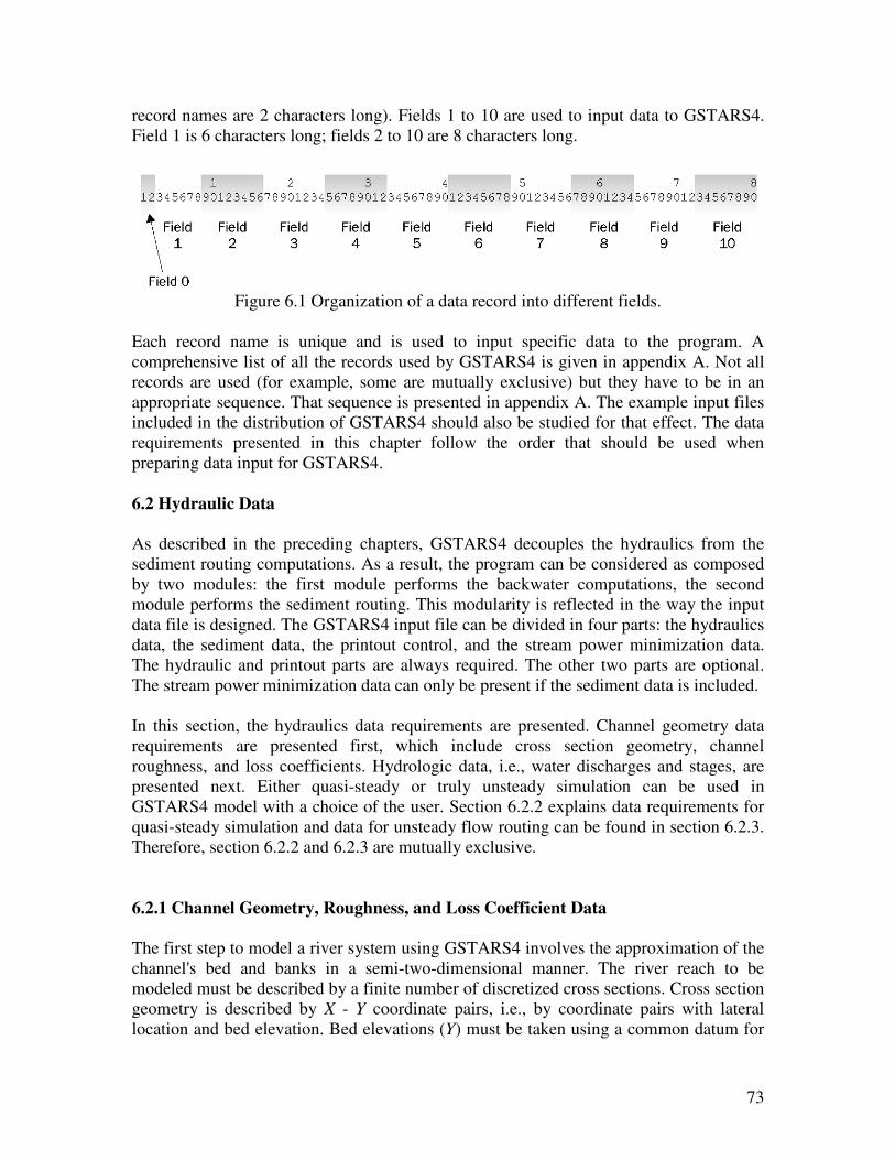
73
record names are 2 characters long). Fields 1 to 10 are used to input data to GSTARS4.
Field 1 is 6 characters long; fields 2 to 10 are 8 characters long.
Figure 6.1 Organization of a data record into different fields.
Each record name is unique and is used to input specific data to the program. A
comprehensive list of all the records used by GSTARS4 is given in appendix A. Not all
records are used (for example, some are mutually exclusive) but they have to be in an
appropriate sequence. That sequence is presented in appendix A. The example input files
included in the distribution of GSTARS4 should also be studied for that effect. The data
requirements presented in this chapter follow the order that should be used when
preparing data input for GSTARS4.
6.2 Hydraulic Data
As described in the preceding chapters, GSTARS4 decouples the hydraulics from the
sediment routing computations. As a result, the program can be considered as composed
by two modules: the first module performs the backwater computations, the second
module performs the sediment routing. This modularity is reflected in the way the input
data file is designed. The GSTARS4 input file can be divided in four parts: the hydraulics
data, the sediment data, the printout control, and the stream power minimization data.
The hydraulic and printout parts are always required. The other two parts are optional.
The stream power minimization data can only be present if the sediment data is included.
In this section, the hydraulics data requirements are presented. Channel geometry data
requirements are presented first, which include cross section geometry, channel
roughness, and loss coefficients. Hydrologic data, i.e., water discharges and stages, are
presented next. Either quasi-steady or truly unsteady simulation can be used in
GSTARS4 model with a choice of the user. Section 6.2.2 explains data requirements for
quasi-steady simulation and data for unsteady flow routing can be found in section 6.2.3.
Therefore, section 6.2.2 and 6.2.3 are mutually exclusive.
6.2.1 Channel Geometry, Roughness, and Loss Coefficient Data
The first step to model a river system using GSTARS4 involves the approximation of the
channel's bed and banks in a semi-two-dimensional manner. The river reach to be
modeled must be described by a finite number of discretized cross sections. Cross section
geometry is described by X - Y coordinate pairs, i.e., by coordinate pairs with lateral
location and bed elevation. Bed elevations (Y) must be taken using a common datum for
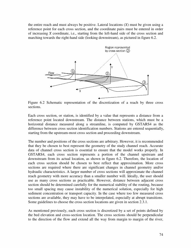
74
the entire reach and must always be positive. Lateral locations (X) must be given using a
reference point for each cross section, and the coordinate pairs must be entered in order
of increasing X coordinate, i.e., starting from the left-hand side of the cross section and
marching towards the right-hand side (looking downstream), as pictured in figure 6.2.
Figure 6.2 Schematic representation of the discretization of a reach by three cross
sections.
Each cross section, or station, is identified by a value that represents a distance from a
reference point located downstream. The distance between stations, which must be a
horizontal distance measured along a streamline, is computed by GSTARS4 as the
difference between cross section identification numbers. Stations are entered sequentially,
starting from the upstream-most cross section and proceeding downstream.
The number and positions of the cross sections are arbitrary. However, it is recommended
that they be chosen to best represent the geometry of the study channel reach. Accurate
data of channel cross section is essential to ensure that the model works properly. In
GSTARS4, each cross section represents a portion of the channel upstream and
downstream from its actual location, as shown in figure 6.2. Therefore, the location of
each cross section should be chosen to best reflect that approximation. More cross
sections are required where there are significant changes in channel geometry and/or
hydraulic characteristics. A larger number of cross sections will approximate the channel
reach geometry with more accuracy than a smaller number will. Ideally, the user should
use as many cross sections as practicable. However, distance between adjacent cross
section should be determined carefully for the numerical stability of the routing, because
too small spacing may cause instability of the numerical solution, especially for high
sediment concentration or transport capacity. In the case where too few measured cross
sections are available, they may have to be interpolated, especially at abrupt transitions.
Some guidelines to choose the cross section locations are given in section 2.3.1.
As mentioned previously, each cross section is discretized by a set of points defined by
the bed elevation and cross-section location. The cross sections should be perpendicular
to the direction of the flow and extend all the way from margin to margin of the river,
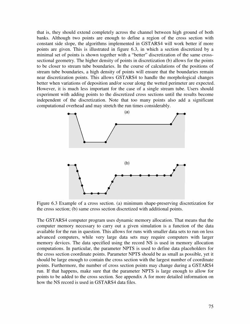
75
that is, they should extend completely across the channel between high ground of both
banks. Although two points are enough to define a region of the cross section with
constant side slope, the algorithms implemented in GSTARS4 will work better if more
points are given. This is illustrated in figure 6.3, in which a section discretized by a
minimal set of points is shown together with a “better” discretization of the same cross-
sectional geometry. The higher density of points in discretization (b) allows for the points
to be closer to stream tube boundaries. In the course of calculations of the positions of
stream tube boundaries, a high density of points will ensure that the boundaries remain
near discretization points. This allows GSTARS4 to handle the morphological changes
better when variations of deposition and/or scour along the wetted perimeter are expected.
However, it is much less important for the case of a single stream tube. Users should
experiment with adding points to the discretized cross sections until the results become
independent of the discretization. Note that too many points also add a significant
computational overhead and may stretch the run times considerably.
Figure 6.3 Example of a cross section. (a) minimum shape-preserving discretization for
the cross section; (b) same cross section discretized with additional points.
The GSTARS4 computer program uses dynamic memory allocation. That means that the
computer memory necessary to carry out a given simulation is a function of the data
available for the run in question. This allows for runs with smaller data sets to run on less
advanced computers, while very large data sets may require computers with larger
memory devices. The data specified using the record NS is used in memory allocation
computations. In particular, the parameter NPTS is used to define data placeholders for
the cross section coordinate points. Parameter NPTS should be as small as possible, yet it
should be large enough to contain the cross section with the largest number of coordinate
points. Furthermore, the number of cross section points may change during a GSTARS4
run. If that happens, make sure that the parameter NPTS is large enough to allow for
points to be added to the cross section. See appendix A for more detailed information on
how the NS record is used in GSTARS4 data files.
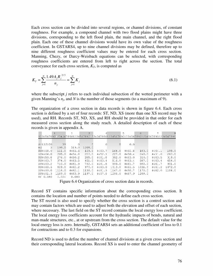
76
Each cross section can be divided into several regions, or channel divisions, of constant
roughness. For example, a compound channel with two flood plains might have three
divisions, corresponding to the left flood plain, the main channel, and the right flood
plain. Each one of these channel divisions would have its own value of the roughness
coefficient. In GSTARS4, up to nine channel divisions may be defined, therefore up to
nine different roughness coefficient values may be entered for each cross section.
Manning, Chezy, or Darcy-Weisbach equations can be selected, with corresponding
roughness coefficients are entered from left to right across the section. The total
conveyance for each cross section, KT, is computed as
∑∑==
==N
j
j
N
j j
jj
T Kn
RAK
11
3/249.1
(6.1)
where the subscript j refers to each individual subsection of the wetted perimeter with a
given Manning’s nj, and N is the number of those segments (to a maximum of 9).
The organization of a cross section in data records is shown in figure 6.4. Each cross
section is defined by a set of four records: ST, ND, XS (more than one XS record may be
used), and RH. Records ST, ND, XS, and RH should be provided in that order for each
measured cross section along the study reach. A detailed description of each of these
records is given in appendix A.
Figure 6.4 Organization of cross section data in records.
Record ST contains specific information about the corresponding cross section. It
contains the location and number of points needed to define each cross section.
The ST record is also used to specify whether the cross section is a control section and
may contain factors which are used to adjust both the elevation and offset of each section,
where necessary. The last field on the ST record contains the local energy loss coefficient.
The local energy loss coefficients account for the hydraulic impacts of bends, natural and
man-made structures, etc., at or upstream from the cross section. The default value for the
local energy loss is zero. Internally, GSTARS4 sets an additional coefficient of loss to 0.1
for contractions and to 0.3 for expansions.
Record ND is used to define the number of channel divisions at a given cross section and
their corresponding lateral locations. Record XS is used to enter the channel geometry of
77
a given station using x-y (or y-x) coordinate pairs. The RH record defines the roughness
coefficient of each channel division identified on the preceding ND record of the cross
section.
GSTARS4 can use the Manning, Darcy-Weisbach, or Chezy equations for energy slope
and conveyance computations. The desired equation must be selected using one RE
record, which must be present after the channel geometry data. If the RE record is not
included in the data set, the program will default to Manning's equation. The RE record is
also used to specify the equation employed to compute the local friction slope.
6.2.2 Discharge and Stage Data for Quasi-steady Flow Simulation
The hydraulic data necessary for a numerical simulation are water stages and
corresponding surface elevation at certain points (boundary conditions). In GSTARS4,
the inflow discharge hydrograph entering the study reach, i.e., at the station farthest
upstream, must be given for the period of the analysis. As with any steady state model,
the hydrograph must be approximated by bursts of constant discharge and finite duration.
For subcritical open channel flow, the water stage hydrograph must be given for the
station farthest downstream. In GSTARS4, the exception is for reservoir operations,
where the discharge rather than the stage is prescribed at the dam. As described in section
5.1, the discharge information is used to determine the water stage at the reservoir. In all
other cases, the stage for the downstream-most cross section must be given. A
supercritical downstream boundary condition should not be used.
Discharge hydrographs are given in tables with the discretized values in multiples of a
fixed time increment, i.e., of the time step. Corresponding water surface elevations are
given either in tabular format or as stage-discharge rating curves. The type of input for
the water discharges is chosen by defining the value of IOPTQ in record QQ, and the
type of input for the corresponding stages is chosen by defining the value of IOPTSTQ in
record SS. The possible options are summarized in table 6.1. The data is then entered
using records IT, QQ, SS, DD, SQ, TL, TQ, RC, NC, DR, HR, and RQ. Depending on
the option chosen, some of these records may be omitted. Detailed descriptions of these
records are given in appendix A.
Table 6.1 Records required for each combination of QQ and SS record selections. The
numbers in parentheses correspond to the sections where each case is described.

78
6.2.2.1 Discharge Hydrograph with a Stage-Discharge Rating Curve
In this case, the water discharges for the reach are given in the form of a hydrograph, and
the corresponding water stages are given as a rating curve, i.e., as a function of the
discharge. This option is selected by using the RATING CURVE option in record SS and
the DISCRETIZED DISCHARGES option in record QQ. The discretized hydrograph is
entered using DD records, and the water stage is defined by a rating curve using records
NC and RC.
The discretization of the hydrograph is a process that transforms a continuous curve into
discrete numerical values with a certain discharge and time duration. The continuous
curve is then replaced by a stair-stepping curve with constant discharge bursts with a
duration that, in GSTARS4, must be a whole multiple of the time step, ∆t. The process is
briefly illustrated in figure 6.5. First, a time interval must be chosen for the time step, ∆t.
It must be small enough so that all the important features of the hydrograph may be
preserved without significant distortion. Using ∆t, the hydrograph is broken into intervals
of constant discharge. The duration of each of these intervals is expressed as whole
multiples of ∆t.
As an example of this procedure, a hypothetical hydrograph is given as a continuous,
smooth line in figure 6.5. A time step ∆t = 1 day is chosen to discretize the hydrograph.
The hydrograph is then replaced by the stair-stepping curve representing the following
discharge bursts: one time step of Q1, one time step of Q2, one time step of Q3, one time
step of Q4, two time steps of Q5, two time steps of Q6, and one time step of Q7 discharges.
A total of 7 discharges are used, but 9 time steps must be carried out by the simulation.
These values will be entered in DD records, as shown below. Note that a smaller time
step could have been used. This would have resulted in a more accurate representation of
the hydrograph, but more time steps would have to be computed by the program,
resulting in longer computational times.
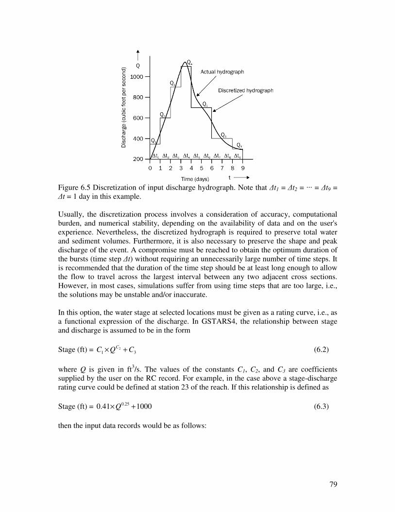
79
Figure 6.5 Discretization of input discharge hydrograph. Note that ∆t1 = ∆t2 = ··· = ∆t9 =
∆t = 1 day in this example.
Usually, the discretization process involves a consideration of accuracy, computational
burden, and numerical stability, depending on the availability of data and on the user's
experience. Nevertheless, the discretized hydrograph is required to preserve total water
and sediment volumes. Furthermore, it is also necessary to preserve the shape and peak
discharge of the event. A compromise must be reached to obtain the optimum duration of
the bursts (time step ∆t) without requiring an unnecessarily large number of time steps. It
is recommended that the duration of the time step should be at least long enough to allow
the flow to travel across the largest interval between any two adjacent cross sections.
However, in most cases, simulations suffer from using time steps that are too large, i.e.,
the solutions may be unstable and/or inaccurate.
In this option, the water stage at selected locations must be given as a rating curve, i.e., as
a functional expression of the discharge. In GSTARS4, the relationship between stage
and discharge is assumed to be in the form
Stage (ft) = 312 CQC
C +× (6.2)
where Q is given in ft3/s. The values of the constants C1, C2, and C3 are coefficients
supplied by the user on the RC record. For example, in the case above a stage-discharge
rating curve could be defined at station 23 of the reach. If this relationship is defined as
Stage (ft) = 100041.0 25.0 +×Q (6.3)
then the input data records would be as follows:

80
Note that the sum of all the time steps defined in the first column of the DD records
(NDAYS in field 1 of DD records) must be equal to the total number of time steps for the
run (ITIMAX in field 1 of the IT record), which, in this case, is 9 time steps for 9 days.
6.2.2.2 Table of Discharges with a Rating Curve at The Control Section
This type of input is a particular form of the input described above. It may be useful when
discharges are known from periodic records, at fixed time intervals, in the form of a table.
This option is selected by using the RATING CURVE option in record SS and the
TABLE OF DISCHARGES option in record QQ. The table is entered using TQ records,
and the water stage is defined by a rating curve using records NC and RC.
As an example, consider the following table of daily discharges which could have been
obtained from a gaging station at the upstream end of the study reach:
With the same stage-discharge rating curve in the example of the previous section, the
input data records would be:

81
Additional TQ records may be supplied for longer simulations.
6.2.2.3 Stage-Discharge Table at a Control Section
In this case, the information for the control station is given in a table with discharges and
corresponding water stages. This option is selected by using the STAGE DISCHARGE
TABLE option in record SS and the TABLE OF DISCHARGES option in record QQ.
The table is entered using TL and SQ records. As an example, consider the information
given in the table below, which could have been obtained from a gaging station at the
control section located at section 35:
For daily time steps, the input data records for this example would be:

82
6.2.2.4 Reservoir Routing with Table of Discharges
Usually, in reservoir routing the outflow through the dam differs from the river inflow to
the reservoir. In this case, the discharge at the dam is given, from which level pool
routing is used to compute the stage there. Backwater computations can thus proceed
upstream, starting at the dam. The dam is always located at the last cross section, i.e., at
the downstream-most cross section of the reach.
To illustrate the use of reservoir routing calculations in GSTARS4 using one table of
discharges, consider the hydrographs in figure 6.6. The river discharge (inflow to the
reservoir) is given as a solid line, and the outflow through the dam is given in a dotted
line. A uniform time step ∆t = 1 day is used. A possible discretization of the hydrographs,
also shown in the same figure, is the following:
Figure 6.6 Idealized inflow and outflow hydrographs for reservoir routing calculations,
with the corresponding discretized stepped hydrographs.
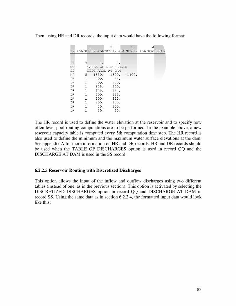
83
Then, using HR and DR records, the input data would have the following format:
The HR record is used to define the water elevation at the reservoir and to specify how
often level-pool routing computations are to be performed. In the example above, a new
reservoir capacity table is computed every 5th computation time step. The HR record is
also used to define the minimum and the maximum water surface elevations at the dam.
See appendix A for more information on HR and DR records. HR and DR records should
be used when the TABLE OF DISCHARGES option is used in record QQ and the
DISCHARGE AT DAM is used in the SS record.
6.2.2.5 Reservoir Routing with Discretized Discharges
This option allows the input of the inflow and outflow discharges using two different
tables (instead of one, as in the previous section). This option is activated by selecting the
DISCRETIZED DISCHARGES option in record QQ and DISCHARGE AT DAM in
record SS. Using the same data as in section 6.2.2.4, the formatted input data would look
like this:
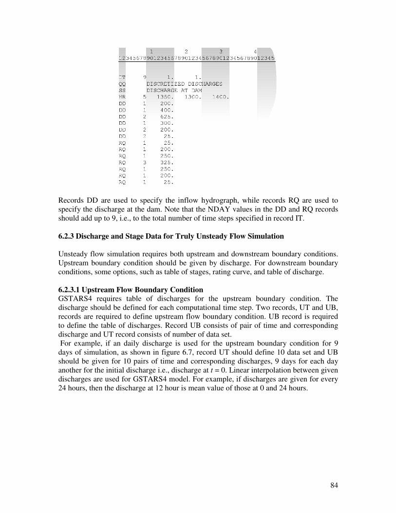
84
Records DD are used to specify the inflow hydrograph, while records RQ are used to
specify the discharge at the dam. Note that the NDAY values in the DD and RQ records
should add up to 9, i.e., to the total number of time steps specified in record IT.
6.2.3 Discharge and Stage Data for Truly Unsteady Flow Simulation
Unsteady flow simulation requires both upstream and downstream boundary conditions.
Upstream boundary condition should be given by discharge. For downstream boundary
conditions, some options, such as table of stages, rating curve, and table of discharge.
6.2.3.1 Upstream Flow Boundary Condition
GSTARS4 requires table of discharges for the upstream boundary condition. The
discharge should be defined for each computational time step. Two records, UT and UB,
records are required to define upstream flow boundary condition. UB record is required
to define the table of discharges. Record UB consists of pair of time and corresponding
discharge and UT record consists of number of data set.
For example, if an daily discharge is used for the upstream boundary condition for 9
days of simulation, as shown in figure 6.7, record UT should define 10 data set and UB
should be given for 10 pairs of time and corresponding discharges, 9 days for each day
another for the initial discharge i.e., discharge at t = 0. Linear interpolation between given
discharges are used for GSTARS4 model. For example, if discharges are given for every
24 hours, then the discharge at 12 hour is mean value of those at 0 and 24 hours.

85
0
100
200
300
400
500
600
700
800
900
0 24 48 72 96 120 144 168 192 216
Time (hours)
Dis
ch
arg
e (
cfs
)
Figure 6.7 Hydrograph for the upstream boundary condition with computation time step
for 24 hour, ∆t = 24 hour.
Then, record UT should define 10 set would be used and 10 lines of UB records have to
be given, the input data records for the upstream flow boundary would be:
1 2
1 2 3 4 5 6 7 8 9 0 1 2 3 4 5 6 7 8 9 0 1 2 3 4
U T 2 1 0
U B 0 1 0 0
U B 2 4 2 5 0
U B 4 8 3 5 0
U B 7 2 5 5 0
U B 9 6 8 5 0
U B 1 2 0 7 0 0
U B 1 4 4 6 0 0
U B 1 6 8 3 0 0
U B 1 9 2 1 0 0
U B 2 1 6 5 0
Time for record UB should be hour only. Field 1 of record UT should be 2 for GSTARS4
version.
6.2.3.2 Downstream Flow Boundary Condition
A data set for the downstream boundary condition is required for an unsteady flow
simulation.
GSTARS4 has capability using three options for the downstream boundary condition,
table of stage, table of discharge, and rating curve. One among these three options should
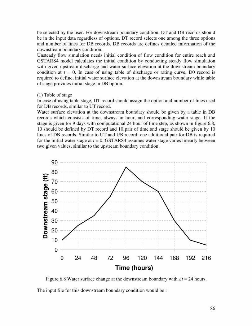
86
be selected by the user. For downstream boundary condition, DT and DB records should
be in the input data regardless of options. DT record selects one among the three options
and number of lines for DB records. DB records are defines detailed information of the
downstream boundary condition.
Unsteady flow simulation needs initial condition of flow condition for entire reach and
GSTARS4 model calculates the initial condition by conducting steady flow simulation
with given upstream discharge and water surface elevation at the downstream boundary
condition at t = 0. In case of using table of discharge or rating curve, D0 record is
required to define, initial water surface elevation at the downstream boundary while table
of stage provides initial stage in DB option.
(1) Table of stage
In case of using table stage, DT record should assign the option and number of lines used
for DB records, similar to UT record.
Water surface elevation at the downstream boundary should be given by a table in DB
records which consists of time, always in hour, and corresponding water stage. If the
stage is given for 9 days with computational 24 hour of time step, as shown in figure 6.8,
10 should be defined by DT record and 10 pair of time and stage should be given by 10
lines of DB records. Similar to UT and UB record, one additional pair for DB is required
for the initial water stage at t = 0. GSTARS4 assumes water stage varies linearly between
two given values, similar to the upstream boundary condition.
0
10
20
30
40
50
60
70
80
90
0 24 48 72 96 120 144 168 192 216
Time (hours)
Do
wn
str
eam
sta
ge (
ft)
Figure 6.8 Water surface change at the downstream boundary with ∆t = 24 hours.
The input file for this downstream boundary condition would be :

87
1 2
1 2 3 4 5 6 7 8 9 0 1 2 3 4 5 6 7 8 9 0 1 2 3 4
D T 1 1 0
D B 0 1 0
D B 2 4 2 5
D B 4 8 3 5
D B 7 2 5 5
D B 9 6 8 5
D B 1 2 0 7 0
D B 1 4 4 6 0
D B 1 6 8 3 0
D B 1 9 2 1 0
D B 2 1 6 5
“1” at the first field of DT record is option for table of stage.
(2) Table of Discharge
Option of table of discharge is almost the same as that of table of stage. DT record
includes selection of the option and number of data pairs of DB. DB records consist of
time and corresponding water discharge. Linear interpretation is also used for
downstream discharge table also by GSTARS4.
For the initial flow condition along the reach, an additional D0 record, including the stage
at t = 0. For example, the downstream discharge is given by figure 6.9 with initial water
stage of 15 ft.
0
10
20
30
40
50
60
70
80
90
0 24 48 72 96 120 144 168 192 216
Time (hours)
Do
wn
str
eam
dis
ch
arg
e (
cfs
)
Figure 6.9 Hydrograph for the downstream boundary condition with ∆t = 24 hour.
Then the input file for the downstream boundary condition would be :

88
1 2
1 2 3 4 5 6 7 8 9 0 1 2 3 4 5 6 7 8 9 0 1 2 3 4
D T 2 1 0
D 0 1 5
D B 0 1 0 0
D B 2 4 2 5 0
D B 4 8 3 5 0
D B 7 2 5 5 0
D B 9 6 8 5 0
D B 1 2 0 7 0 0
D B 1 4 4 6 0 0
D B 1 6 8 3 0 0
D B 1 9 2 1 0 0
D B 2 1 6 5 0
“2” at the first field of DT record is option for table of stage.
(3) Rating Curve
Eq. (6.2) can be used as downstream boundary condition for unsteady flow simulation.
Similar to table of discharge, D0 record should be given to define and compute the initial
flow condition. For example, rating curve of Eq. (6.3) is used for the downstream
boundary condition with 15 ft of initial water stage at the downstream boundary. Then
the input data would be :
1 2 3
1 2 3 4 5 6 7 8 9 0 1 2 3 4 5 6 7 8 9 0 1 2 3 4 5 6 7 8 9 0 1 2
D T 9 1
D 0 1 5
D B 0 . 4 1 0 . 2 5 1 0 0 0
“9” and “1” at the first and the second field of DT record represents option for rating
curve and 1 line for DB record, respectively.
6.3 Sediment Data
The information presented in the last section is enough to have GSTARS4 performing
backwater computations in a channel with fixed bed. If, however, sediment routing is
required, sediment data must be given to the model. Sediment data includes bed material
size distributions for the reach of study and the sediment inflow hydrograph entering the
reach, including its particle size distribution. The input data requirements (and
corresponding records) for sediment routing computations are presented in this section.
The sediment transport computations are activated by inclusion of the SE record in the
input data file. The SE record is used to select the equation for computing sediment
transport capacities. In GSTARS4, sediment transport capacities can be determined by
any of the methods in table 6.2. Desired sediment transport equations can be selected by
the variable ISED in the SE record. These methods were chosen because of their
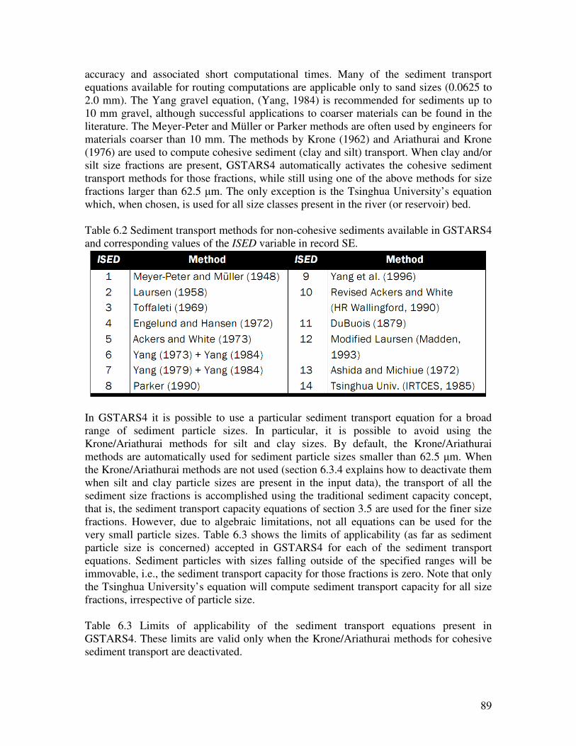
89
accuracy and associated short computational times. Many of the sediment transport
equations available for routing computations are applicable only to sand sizes (0.0625 to
2.0 mm). The Yang gravel equation, (Yang, 1984) is recommended for sediments up to
10 mm gravel, although successful applications to coarser materials can be found in the
literature. The Meyer-Peter and Müller or Parker methods are often used by engineers for
materials coarser than 10 mm. The methods by Krone (1962) and Ariathurai and Krone
(1976) are used to compute cohesive sediment (clay and silt) transport. When clay and/or
silt size fractions are present, GSTARS4 automatically activates the cohesive sediment
transport methods for those fractions, while still using one of the above methods for size
fractions larger than 62.5 µm. The only exception is the Tsinghua University’s equation
which, when chosen, is used for all size classes present in the river (or reservoir) bed.
Table 6.2 Sediment transport methods for non-cohesive sediments available in GSTARS4
and corresponding values of the ISED variable in record SE.
In GSTARS4 it is possible to use a particular sediment transport equation for a broad
range of sediment particle sizes. In particular, it is possible to avoid using the
Krone/Ariathurai methods for silt and clay sizes. By default, the Krone/Ariathurai
methods are automatically used for sediment particle sizes smaller than 62.5 µm. When
the Krone/Ariathurai methods are not used (section 6.3.4 explains how to deactivate them
when silt and clay particle sizes are present in the input data), the transport of all the
sediment size fractions is accomplished using the traditional sediment capacity concept,
that is, the sediment transport capacity equations of section 3.5 are used for the finer size
fractions. However, due to algebraic limitations, not all equations can be used for the
very small particle sizes. Table 6.3 shows the limits of applicability (as far as sediment
particle size is concerned) accepted in GSTARS4 for each of the sediment transport
equations. Sediment particles with sizes falling outside of the specified ranges will be
immovable, i.e., the sediment transport capacity for those fractions is zero. Note that only
the Tsinghua University’s equation will compute sediment transport capacity for all size
fractions, irrespective of particle size.
Table 6.3 Limits of applicability of the sediment transport equations present in
GSTARS4. These limits are valid only when the Krone/Ariathurai methods for cohesive
sediment transport are deactivated.

90
The selection of the appropriate sediment transport function remains an unsolved
problem. Differences in the assumptions used to derive the equations, study of published
data, and practical reasoning and experience are factors that can help in this process.
There are tremendous uncertainties involved in estimating sediment discharge under
different flow and sediment conditions and under different hydrologic, geologic, and
climatic constraints. It is very difficult to recommend a particular equation or method to
be used under all circumstances. The following guidelines are based on those given by
Yang (1996, 2003) and were adapted for inclusion in the present manual:
1 Use as much field and measured data as possible, within the time, budget, and
manpower limits of each particular study.
2 Examine as many formulae as possible, based on assumptions used in their derivation
and range of data used to determine its coefficients, and select those consistent with the
data and measurements obtained in step 1.
3 If more than one formula survived step 2, compute sediment transport rates with these
formulae and select those that best agree with any field measurements taken in step 1.
4 In the absence of measured sediment loads for comparison, the following guidelines
could be considered:
· Use Meyer-Peter and Müller's formula when the bed material is coarser than 5 mm.
· Use Toffaleti's formula for large sand-bed rivers.
· Use Yang's (1973) formula for sand transport in laboratory flumes and natural rivers;
use Yang's (1979) formula for sand transport when the critical unit stream power at
incipient motion can be neglected.
· Use Parker's (1990) or Yang's (1984) gravel formulae for bed load or gravel transport;
· Use Yang's (1996) modified formula for high-concentration flows when the wash load
or concentration of fine material is high.

91
· Use Ackers and White's or Engelund and Hansen's formulae for subcritical flow
condition in the lower flow regime.
· Use Laursen's formula for laboratory flumes and shallow rivers with fine sand or
coarse silt.
GSTARS4 users may also consider using Yang and Huang’s (2001) analyses included in
appendix D, as a reference in the selection of sediment transport formulae.
6.3.1 Sediment Inflow Data
The inflow sediment hydrograph must be given for the section farthest upstream from the
study reach. In GSTARS4, this can be given in the form of either discretized sediment
discharges on QS records or a sediment rating curve using record QR. It can also be
indirectly obtained by using an equilibrium condition at the upstream-most station, in
which sediment inflow is set to the sediment transport capacity of the cross section. In the
first case, the sediment rating curve has to be discretized following a procedure similar to
that described in section 6.2.2.1 for the water discharge hydrograph. The data is entered
using QS records, which follow the same format as the DD records described above.
Alternatively, a sediment rating curve, if known, may be given using a QR record. This
record allows the user to specify a sediment discharge that is a function of the water
discharge in the form
b
s aQQ = (6.4)
where Qs = incoming sediment discharge (in ton/day); Q = water discharge (ft3 /s); and a
and b are coefficients to be supplied in the QR record (a, b > 0). For example, if it is
known that the incoming sediment discharge is a function of the water discharge such
that
2.14.0 QQs = (6.5)
the input QR record would take the following format:
An alternative way to specify the sediment inflow and its distribution is to use an
equilibrium first station. In this case, the definition of equilibrium is that the cross section
geometry and bed gradation distribution do not change during the simulation run. The
inflow sediment transport rate and its distribution can thus be calculated directly from the
sediment transport equation selected in the SE record. In GSTARS4, this method can
only be applied in the cases that do not involve cohesive sediment transport, because the
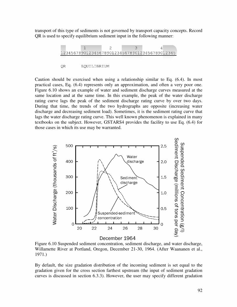
92
transport of this type of sediments is not governed by transport capacity concepts. Record
QR is used to specify equilibrium sediment input in the following manner:
Caution should be exercised when using a relationship similar to Eq. (6.4). In most
practical cases, Eq. (6.4) represents only an approximation, and often a very poor one.
Figure 6.10 shows an example of water and sediment discharge curves measured at the
same location and at the same time. In this example, the peak of the water discharge
rating curve lags the peak of the sediment discharge rating curve by over two days.
During that time, the trends of the two hydrographs are opposite (increasing water
discharge and decreasing sediment load). Sometimes, it is the sediment rating curve that
lags the water discharge rating curve. This well known phenomenon is explained in many
textbooks on the subject. However, GSTARS4 provides the facility to use Eq. (6.4) for
those cases in which its use may be warranted.
Figure 6.10 Suspended sediment concentration, sediment discharge, and water discharge,
Willamette River at Portland, Oregon, December 21-30, 1964. (After Waananen et al.,
1971.)
By default, the size gradation distribution of the incoming sediment is set equal to the
gradation given for the cross section farthest upstream (the input of sediment gradation
curves is discussed in section 6.3.3). However, the user may specify different gradation
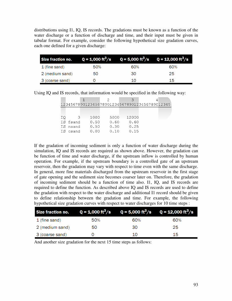
93
distributions using I1, IQ, IS records. The gradations must be known as a function of the
water discharge or a function of discharge and time, and their input must be given in
tabular format. For example, consider the following hypothetical size gradation curves,
each one defined for a given discharge:
Using IQ and IS records, that information would be specified in the following way:
If the gradation of incoming sediment is only a function of water discharge during the
simulation, IQ and IS records are required as shown above. However, the gradation can
be function of time and water discharge, if the upstream inflow is controlled by human
operation. For example, if the upstream boundary is a controlled gate of an upstream
reservoir, then the gradation may vary with respect to time even with the same discharge.
In general, more fine materials discharged from the upstream reservoir in the first stage
of gate opening and the sediment size becomes coarser later on. Therefore, the gradation
of incoming sediment should be a function of time also. I1, IQ, and IS records are
required to define the function. As described above IQ and IS records are used to define
the gradation with respect to the water discharge and additional I1 record should be given
to define relationship between the gradation and time. For example, the following
hypothetical size gradation curves with respect to water discharges for 10 time steps :
And another size gradation for the next 15 time steps as follows:

94
Two I1 records are required, one to define the time 10 time step of the first gradation
curve and another for the next 15 time step, then the formation of I1, IQ, and IS records
would be:
1 2 3
1 2 3 4 5 6 7 8 9 0 1 2 3 4 5 6 7 8 9 0 1 2 3 4 5 6 7 8 9 0 1 2
I 1 1 0
I Q 3 1 0 0 0 5 0 0 0 1 2 0 0 0
I S 0 . 5 0 0 . 6 0 0 . 6 0
I S 0 . 5 0 0 . 3 0 0 . 2 5
I S 0 . 0 0 0 . 1 0 0 . 1 5
I 1 1 5
I Q 3 1 0 0 0 5 0 0 0 1 2 0 0 0
I S 0 . 3 5 0 . 4 0 0 . 4 0
I S 0 . 4 5 0 . 3 5 0 . 3 0
I S 0 . 2 0 0 . 2 5 0 . 3 0
The summation of time steps of I1 records should be identical to the total time step
defined in IT record. The unit for I1 records is also the same unit that defined in IT
records.
GSTARS4 interpolates the gradations for water discharges falling in between the
specified discharges, but does not extrapolate for water discharges outside that range (e.g.,
if the discharge is 13,000 ft3 /s, the distribution specified for Q = 12,000 ft
3/s is used).
GSTARS4 solves the sediment continuity equation, Eq. (3.4), to route sediments through
a channel reach. Eq. (3.4) is discretized following the methods presented in section 3.3,
and computations proceed from upstream to downstream. The incoming sediment
discharge is specified at the first cross section of the reach (the section located at the
upstream end of the reach), therefore a special treatment is necessary there. The reach
length for that section is taken to be half the distance between station 1 and station 2, that
is, ∆xi-1 = 0 in Eq. (3.17). The incoming sediment is used to represent 1, −isQ , and the
solution is the obtained in the usual way. Note that the bed composition of station 1 will,
in general, change with time, therefore the distribution of the incoming sediment should
be specified by the use of I1/IQ/IS sets of records (or by using the equilibrium method
described earlier for the first station). If the distribution of the incoming sediment is not
specified, it is assumed that the distribution of the incoming sediment is identical to that
of the bed at station 1.
45%
35%
20%
35%
40%
25%
30%
40%
30%
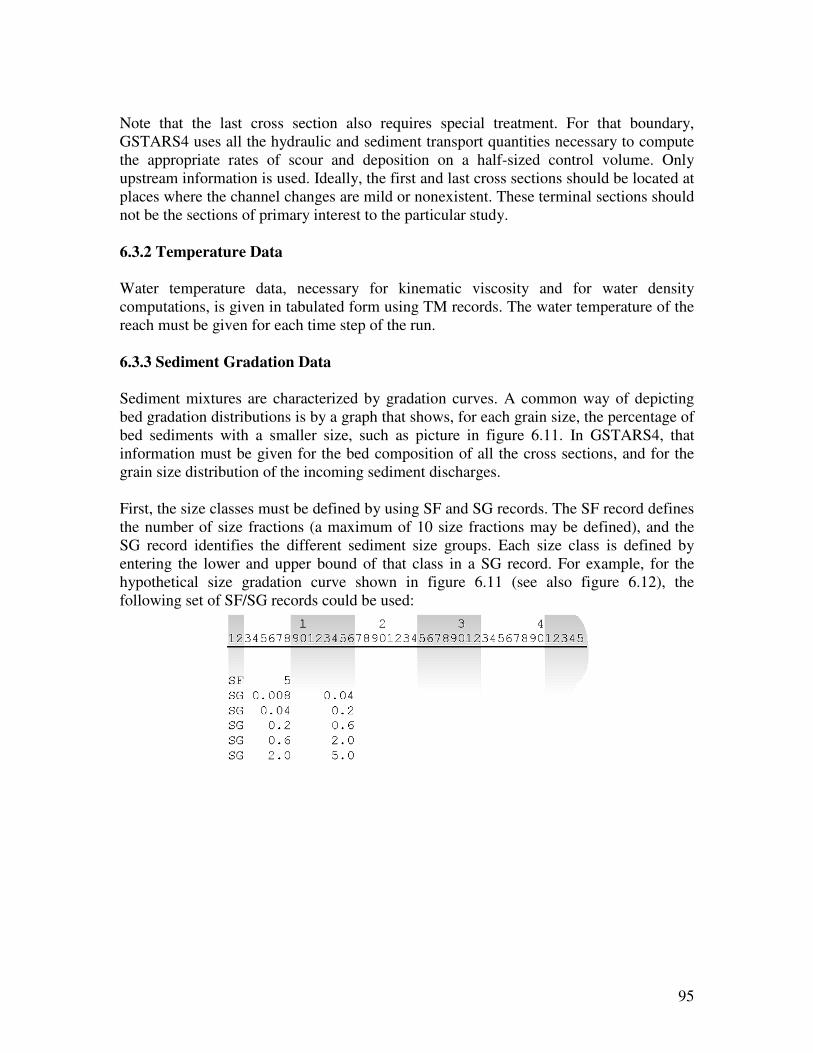
95
Note that the last cross section also requires special treatment. For that boundary,
GSTARS4 uses all the hydraulic and sediment transport quantities necessary to compute
the appropriate rates of scour and deposition on a half-sized control volume. Only
upstream information is used. Ideally, the first and last cross sections should be located at
places where the channel changes are mild or nonexistent. These terminal sections should
not be the sections of primary interest to the particular study.
6.3.2 Temperature Data
Water temperature data, necessary for kinematic viscosity and for water density
computations, is given in tabulated form using TM records. The water temperature of the
reach must be given for each time step of the run.
6.3.3 Sediment Gradation Data
Sediment mixtures are characterized by gradation curves. A common way of depicting
bed gradation distributions is by a graph that shows, for each grain size, the percentage of
bed sediments with a smaller size, such as picture in figure 6.11. In GSTARS4, that
information must be given for the bed composition of all the cross sections, and for the
grain size distribution of the incoming sediment discharges.
First, the size classes must be defined by using SF and SG records. The SF record defines
the number of size fractions (a maximum of 10 size fractions may be defined), and the
SG record identifies the different sediment size groups. Each size class is defined by
entering the lower and upper bound of that class in a SG record. For example, for the
hypothetical size gradation curve shown in figure 6.11 (see also figure 6.12), the
following set of SF/SG records could be used:
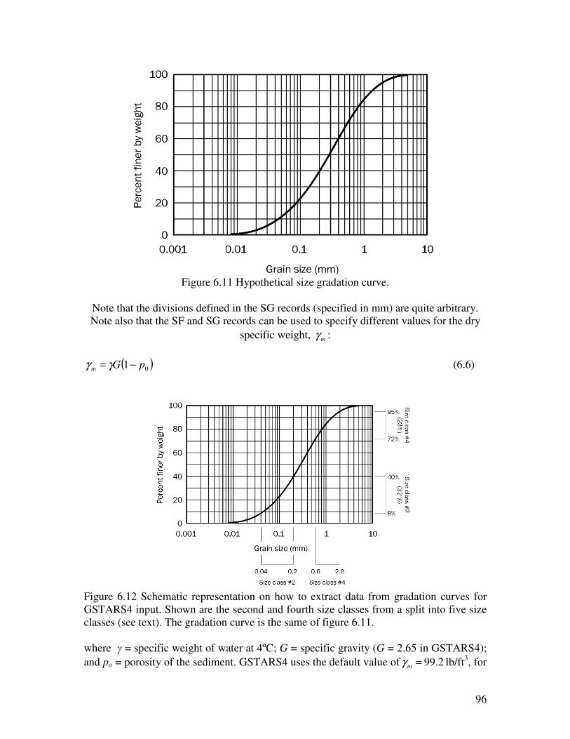
96
Figure 6.11 Hypothetical size gradation curve.
Note that the divisions defined in the SG records (specified in mm) are quite arbitrary.
Note also that the SF and SG records can be used to specify different values for the dry
specific weight, mγ :
( )01 pGm −= γγ (6.6)
Figure 6.12 Schematic representation on how to extract data from gradation curves for
GSTARS4 input. Shown are the second and fourth size classes from a split into five size
classes (see text). The gradation curve is the same of figure 6.11.
where γ = specific weight of water at 4ºC; G = specific gravity (G = 2.65 in GSTARS4);
and po = porosity of the sediment. GSTARS4 uses the default value of 2.99=mγ lb/ft3, for
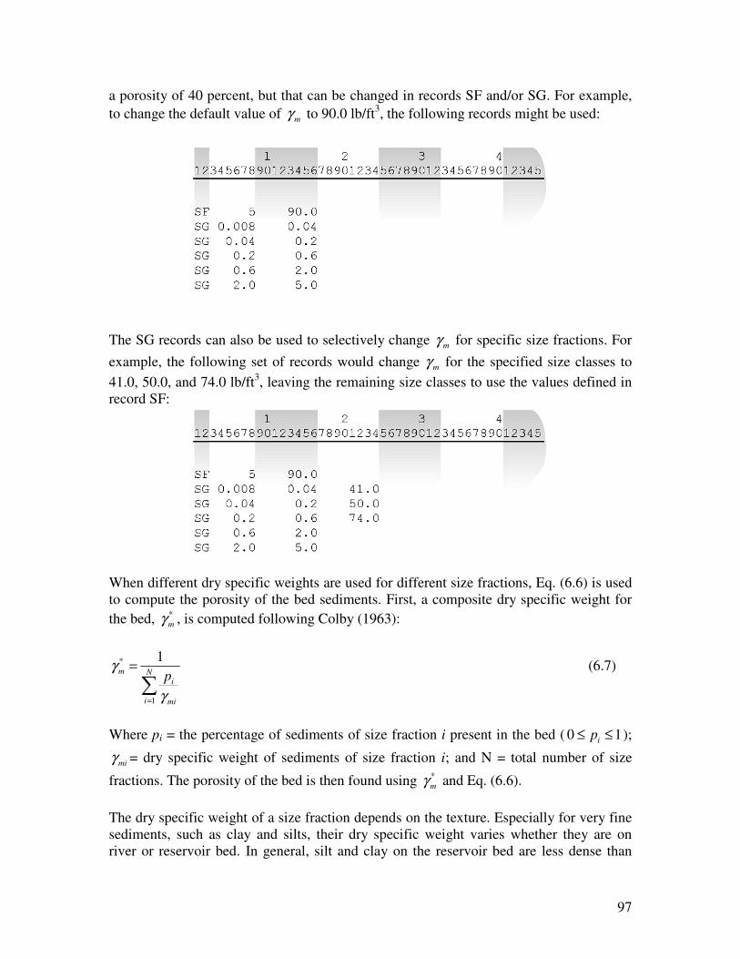
97
a porosity of 40 percent, but that can be changed in records SF and/or SG. For example,
to change the default value of mγ to 90.0 lb/ft3, the following records might be used:
The SG records can also be used to selectively change mγ for specific size fractions. For
example, the following set of records would change mγ for the specified size classes to
41.0, 50.0, and 74.0 lb/ft3, leaving the remaining size classes to use the values defined in
record SF:
When different dry specific weights are used for different size fractions, Eq. (6.6) is used
to compute the porosity of the bed sediments. First, a composite dry specific weight for
the bed, *
mγ , is computed following Colby (1963):
∑=
=N
i mi
i
mp
1
* 1
γ
γ (6.7)
Where pi = the percentage of sediments of size fraction i present in the bed ( 10 ≤≤ ip );
miγ = dry specific weight of sediments of size fraction i; and N = total number of size
fractions. The porosity of the bed is then found using *
mγ and Eq. (6.6).
The dry specific weight of a size fraction depends on the texture. Especially for very fine
sediments, such as clay and silts, their dry specific weight varies whether they are on
river or reservoir bed. In general, silt and clay on the reservoir bed are less dense than

98
those on the river bed (Yang, 1996 and 2003). Therefore, the dry specific weight of each
sediment size group, especially fine materials, should vary with respect to cross section
location, if there is significant change of the flow condition, such as alternation of river
and reservoir. The variation of the dry specific weight with respect to location can be
defined by SL record in GSTARS4. SL record must be specified for each cross section. If
there is 3 sediment size group, each SL record consists of 3 column. In SL records, a SL
record defines dry specific weight of sediment at a cross section, kim ,,γ
mkkikim n γγ ×= ,,, (6.8)
where ni,k = a user specified positive multiplication factor for defining dry specific weight
of size faction k at cross section i. mkγ , dry specific weight of sediments of size fraction k,
given by SF and SG records.
For example, if hypothetical sediment group and their dry specific density are given by
SF and SG records as follows:
1 2
1 2 3 4 5 6 7 8 9 0 1 2 3 4 5 6 7 8 9 0 1 2 3 4
S F 5
S G 0 . 0 0 2 0 . 0 0 4 3 0
S G 0 . 0 0 4 0 . 0 6 2 7 0
S G 0 . 0 6 2 0 . 0 5 0 9 7
If the first sediment size group has dry specific weight of 60lb/ft3 = 2×30lb/ft
3 for only
cross section 1 and 2, then n1 = 2 for cross section 1 and 2. And the dry specific weight
for other size fraction, n2 = n3 = 1, and other cross section, then SL records would be :
1 2 1 2 3 4 5 6 7 8 9 0 1 2 3 4 5 6 7 8 9 0 1 2 3 4
S L 2 . 0 1 . 0 1 . 0
S L 2 . 0 1 . 0 1 . 0
. . . . . .
S L 1 . 0 1 . 0 1 . 0
S L 1 . 0 1 . 0 1 . 0
S L 1 . 0 1 . 0 1 . 0
S L 1 . 0 1 . 0 1 . 0
S L 1 . 0 1 . 0 1 . 0
S L 1 . 0 1 . 0 1 . 0
One SL record is necessary for each cross section, and the data is entered to the
upstream-most cross section and proceeding in the downstream direction. Total number
of SL records should be the same as the number cross section given by record NS
(section 6.2.1).
If there is no significant change of the flow condition or composition of silt or clay is
negligible, there is no need to define variation of the dry specific weight with respect to
cross section location.

99
Gradation information is specified by converting the bed gradation curves into
histograms containing the percentage of sediments in each interval. The process is
schematized in figure 6.12. The data can be specified using either SD records, or sets of
NB and BG records. These records are used to enter the bed material size fractions that
fall within each of the size groups defined by SG records. Using the hypothetical
gradation curve of figure 6.11, the SD records would take the form
One SD record must be specified for each cross section. SC records are similar to SD
records, but they use cumulative values rather than the individual size classes. For
example, the same data of the example above would be entered as
Alternatively, sets of NB and BG records can be used to specify size distributions at
particular locations. These locations do not need to coincide with the defined cross
section locations. GSTARS4 will interpolate bed gradations for the defined cross sections
using the information from the NB and BG records. In this case, a minimum of one
NB/BG set of records must be used. By using this option, one single set of NB and BG
records could be used to define a whole reach (see the record descriptions in appendix A
for more detail).
It is possible to used layered beds with different particle distributions in each layer. In
those cases, multiple SD records must be specified for each cross section, i.e., one SD
record for each cross section and for each bed layer. Additionally, the bottom elevation of
each layer must also be given. As an example, lets consider the case displayed in figure
6.13: the river bed is in layer 1, under which there is a layer of coarser material (layer 2)
and finally a layer of finer material (layer 3). Using that data and SD records, the
formatted data for the particular cross section of figure 6.13 would be
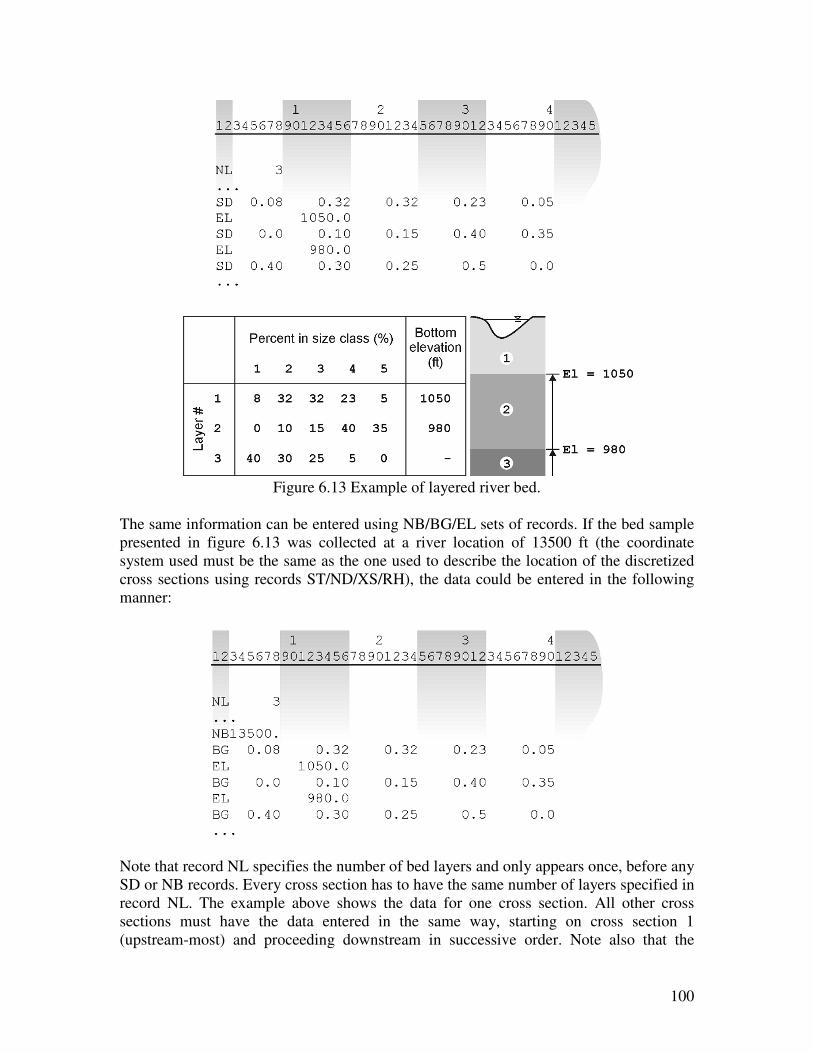
100
Figure 6.13 Example of layered river bed.
The same information can be entered using NB/BG/EL sets of records. If the bed sample
presented in figure 6.13 was collected at a river location of 13500 ft (the coordinate
system used must be the same as the one used to describe the location of the discretized
cross sections using records ST/ND/XS/RH), the data could be entered in the following
manner:
Note that record NL specifies the number of bed layers and only appears once, before any
SD or NB records. Every cross section has to have the same number of layers specified in
record NL. The example above shows the data for one cross section. All other cross
sections must have the data entered in the same way, starting on cross section 1
(upstream-most) and proceeding downstream in successive order. Note also that the
101
lowest layer (last entered data) does not have a bottom elevation: the layer thickness is
assumed to be infinite.
Bed layer distribution information can also be specified using records SC, or NB/BG sets
of records. See appendix A for more detail about how to prepare formatted data for
GSTARS4 using these records.
6.3.3.1 Remarks
The questions that remain are:
1 how to define the intervals for each size class; and
2 how many size classes are needed for each particular study.
Sediment particle size classes should be defined reflecting the well known fact that finer
particles are more important in the sediment transport process than coarser particles.
Therefore, it is reasonable to expect that more classes are necessary in the finer range,
and fewer classes can be used in the coarser range of the distribution. This is, in effect,
what is reflected in the scale used by the American Geophysical Union and presented in
table 6.4. Although the nomenclature and size class definitions in the table are quite
arbitrary, its theoretical background is based on physical principles and approximations
that are convenient follow. Therefore, a similar process can be devised for defining size
classes for use in GSTARS4. Of course that the classes defined in table 6.4 can be used in
GSTARS4, but it will become clear that there are advantages in not always doing it.
The recommended procedure consists in dividing the range of particle sizes such that
they have the same magnitude in the logarithmic space. The process of creating the size
classes can be summarized in the following steps:

102
Table 6.4 Sediment grading scale (Lane, 1947).
1. determine the upper and lower bounds of the particle size ranges to be worked with. If
dmax and dmin are the greatest and the smallest particle diameters encompassing the
particle range, find the values of a and b such that
ad 2min = and b
d 2max =
2. let N be the desired number of size classes for a particular application ( 10≤N ). Select
the lower and upper bound diameters for each interval i in the following way:
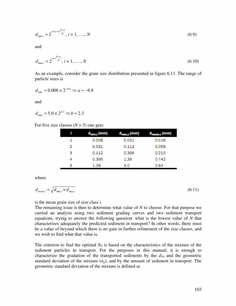
103
N
abia
id
−−+
=)1(
min, 2 , i = 1, …., N (6.9)
and
N
abia
id
−+
= 2max, , i = 1, …., N (6.10)
As an example, consider the grain size distribution presented in figure 6.11. The range of
particle sizes is
8.62008.0 8.6
min −=⇒≅= − ad
and
3.220.5 3.2
max =⇒≅= bd
For five size classes (N = 5) one gets:
where
iiimean ddd max,min,, ×= (6.11)
is the mean grain size of size class i.
The remaining issue is then to determine what value of N to choose. For that purpose we
carried an analysis using two sediment grading curves and two sediment transport
equations, trying to answer the following question: what is the lowest value of N that
characterizes adequately the predicted sediment in transport? In other words, there must
be a value of beyond which there is no gain in further refinement of the size classes, and
we wish to find what that value is.
The criterion to find the optimal N0 is based on the characteristics of the mixture of the
sediment particles in transport. For the purposes in this manual, it is enough to
characterize the gradation of the transported sediments by the d50 and the geometric
standard deviation of the mixture (σg), and by the amount of sediment in transport. The
geometric standard deviation of the mixture is defined as
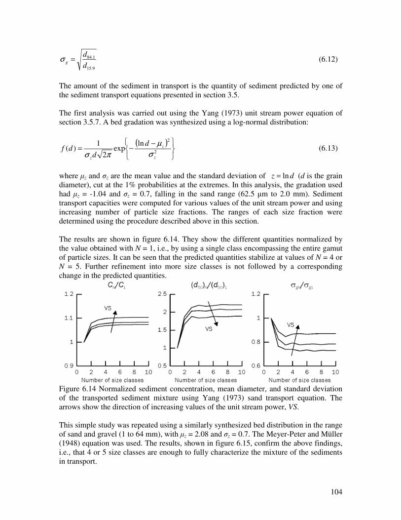
104
9.15
1.84
d
dg =σ (6.12)
The amount of the sediment in transport is the quantity of sediment predicted by one of
the sediment transport equations presented in section 3.5.
The first analysis was carried out using the Yang (1973) unit stream power equation of
section 3.5.7. A bed gradation was synthesized using a log-normal distribution:
( )
−
−=2
2ln
exp2
1)(
z
z
z
d
ddf
σ
µ
πσ (6.13)
where µz and σz are the mean value and the standard deviation of dz ln= (d is the grain
diameter), cut at the 1% probabilities at the extremes. In this analysis, the gradation used
had µz = -1.04 and σz = 0.7, falling in the sand range (62.5 µm to 2.0 mm). Sediment
transport capacities were computed for various values of the unit stream power and using
increasing number of particle size fractions. The ranges of each size fraction were
determined using the procedure described above in this section.
The results are shown in figure 6.14. They show the different quantities normalized by
the value obtained with N = 1, i.e., by using a single class encompassing the entire gamut
of particle sizes. It can be seen that the predicted quantities stabilize at values of N = 4 or
N = 5. Further refinement into more size classes is not followed by a corresponding
change in the predicted quantities.
Figure 6.14 Normalized sediment concentration, mean diameter, and standard deviation
of the transported sediment mixture using Yang (1973) sand transport equation. The
arrows show the direction of increasing values of the unit stream power, VS.
This simple study was repeated using a similarly synthesized bed distribution in the range
of sand and gravel (1 to 64 mm), with µz = 2.08 and σz = 0.7. The Meyer-Peter and Müller
(1948) equation was used. The results, shown in figure 6.15, confirm the above findings,
i.e., that 4 or 5 size classes are enough to fully characterize the mixture of the sediments
in transport.

105
Ultimately, it is up to the user to determine how many size classes (and how to define
them) are needed for the particular study at hand, but the above guidelines should provide
a good starting point for most applications.
Figure 6.15 Normalized sediment concentration, mean diameter, and standard deviation
of the transported sediment mixture using Meyer-Peter and Müller (1948) transport
equation. The arrow shows the direction of increasing values of the bed shear stress, τ.
6.3.4 Cohesive Sediment Transport Parameters
The parameters necessary to model cohesive sediment transport are schematically
represented in figure 6.16. Because these parameters are highly case dependent, and
because they vary within orders of magnitude, GSTARS4 does not assume default values
for these quantities. When modeling cohesive sediment transport, the user should rely on
field data as much as possible.
In figure 6.16, STDEP = shear threshold for deposition of clay and silt; STPERO = shear
threshold for particle erosion of clay and silt; STMERO = shear threshold for mass
erosion of clay and silt; ERMASS = slope of the erosion rate curve for mass erosion; and
ERSTME = Erosion rate of clay and silt when the bed shear stress is equal to STMERO.
Finally, a last parameter is needed, ERLIM, which is the threshold value for the
percentage of clay in the bed composition above which the erosion rates of gravels, sands,
and silts are limited to the erosion rate of clay, as described in section 3.6.2. Values of
ERLIM have been found to have a large range of variation (7% ≤ ERLIM ≤ 80%). These
parameters are formatted using CS or C0 records, as described in appendix A.
The parameters for fall velocities for flocculation and hindered settling are specified
using record CH. The quantities needed are schematically represented in figure 6.17 (see
also section 3.6.1 for further details). Parameters CS1, CS2, CSCOEF1, CSCOEF2,
CSCOEF3, and CSCOEF4 are entered using a single record. Note that parameters CS1
and CS2 are reference concentrations, and they are always given in mg/l, irrespective of
the selected system of units.
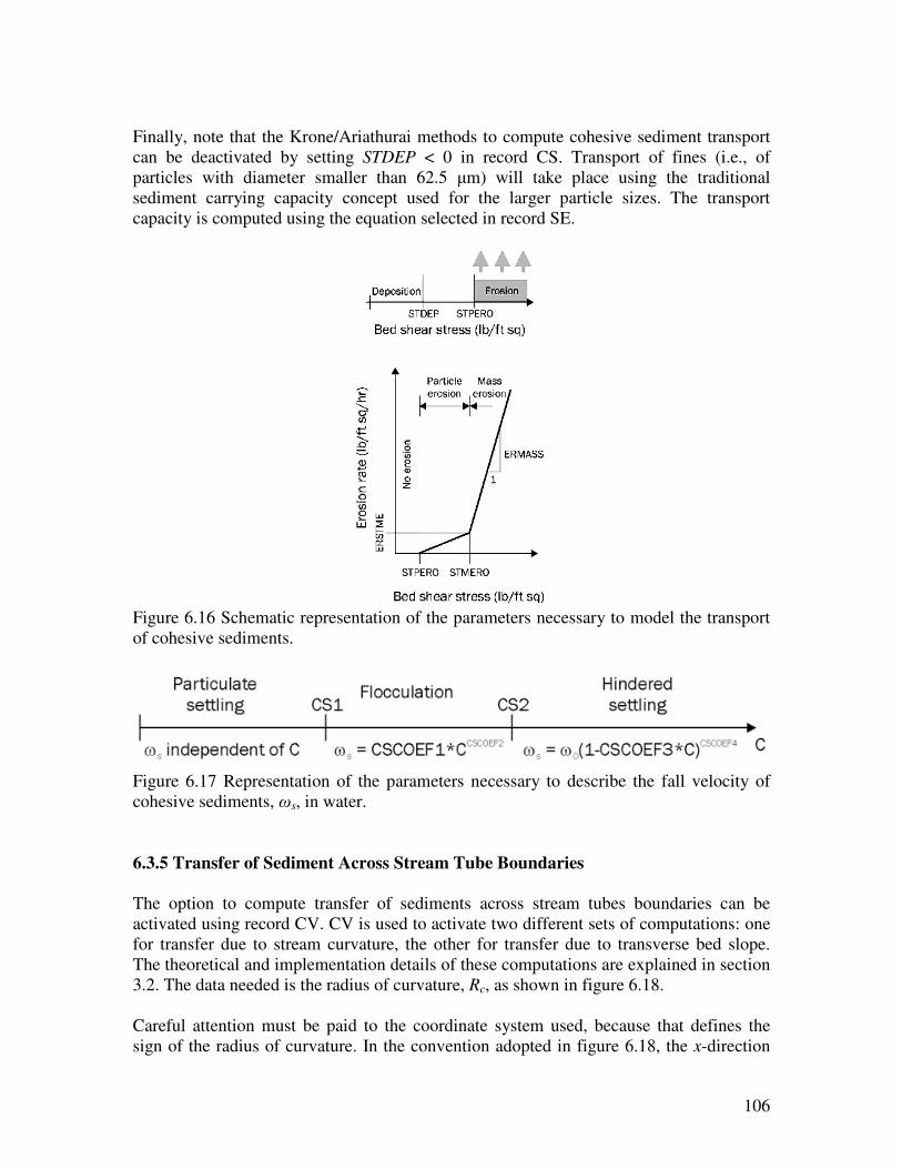
106
Finally, note that the Krone/Ariathurai methods to compute cohesive sediment transport
can be deactivated by setting STDEP < 0 in record CS. Transport of fines (i.e., of
particles with diameter smaller than 62.5 µm) will take place using the traditional
sediment carrying capacity concept used for the larger particle sizes. The transport
capacity is computed using the equation selected in record SE.
Figure 6.16 Schematic representation of the parameters necessary to model the transport
of cohesive sediments.
Figure 6.17 Representation of the parameters necessary to describe the fall velocity of
cohesive sediments, ωs, in water.
6.3.5 Transfer of Sediment Across Stream Tube Boundaries
The option to compute transfer of sediments across stream tubes boundaries can be
activated using record CV. CV is used to activate two different sets of computations: one
for transfer due to stream curvature, the other for transfer due to transverse bed slope.
The theoretical and implementation details of these computations are explained in section
3.2. The data needed is the radius of curvature, Rc, as shown in figure 6.18.
Careful attention must be paid to the coordinate system used, because that defines the
sign of the radius of curvature. In the convention adopted in figure 6.18, the x-direction
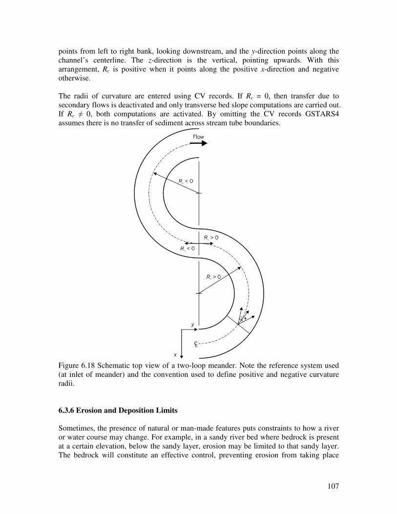
107
points from left to right bank, looking downstream, and the y-direction points along the
channel’s centerline. The z-direction is the vertical, pointing upwards. With this
arrangement, Rc is positive when it points along the positive x-direction and negative
otherwise.
The radii of curvature are entered using CV records. If Rc = 0, then transfer due to
secondary flows is deactivated and only transverse bed slope computations are carried out.
If Rc ≠ 0, both computations are activated. By omitting the CV records GSTARS4
assumes there is no transfer of sediment across stream tube boundaries.
Figure 6.18 Schematic top view of a two-loop meander. Note the reference system used
(at inlet of meander) and the convention used to define positive and negative curvature
radii.
6.3.6 Erosion and Deposition Limits
Sometimes, the presence of natural or man-made features puts constraints to how a river
or water course may change. For example, in a sandy river bed where bedrock is present
at a certain elevation, below the sandy layer, erosion may be limited to that sandy layer.
The bedrock will constitute an effective control, preventing erosion from taking place

108
below its elevation. In GSTARS4, this type of vertical control is specified using LM
records.
To effectively use LM records, knowledge of man-made restrictions to deposition and/or
scour and geological boring data is required. For example, consider the following
hypothetical situation: a channel with bed elevation at 1000 ft is discretized by 5 sections.
A nonerodible bedrock layer at elevation 920 ft is known to exist under the first three
sections, but not thereafter. One LM record is necessary for each cross section, and the
data is entered to the upstream-most cross section and proceeding in the downstream
direction. The LM records for this hypothetical situation would be:
Notice that zero is the lowest bed elevation allowed in GSTARS4. All computations
should be defined such that all vertical bed points have a positive datum at all times of
the run. In practice, the computations will never proceed below the datum line (much like
if an artificial unerodible layer exists at elevation zero). Since no vertical restrictions exist
to deposition, the vertical limits of the example above are simply set to a very high value.
6.4 Output Control
GSTARS4 output is accomplished through column-formatted ASCII files that can be
accessed via a plain ASCII text editor or imported into spreadsheets, such as Microsoft’s
Excel. There are two types of output: hydraulic/sediment parameters and geometry data.
The hydraulic/sediment parameters are organized in files containing flow velocities,
Froude numbers, energy grade line, particle size distributions, etc., for the computational
cross sections in the reach. The geometry data is comprised by tables of thalweg
elevation and water surface elevation versus longitudinal distance, and by cross-sectional
geometries.
Hydraulic/sediment parameter output is controlled in record PR, including the interval at
which the output is desired. There are five possible choices in the control of output using
parameter IPRLVL of record PR:
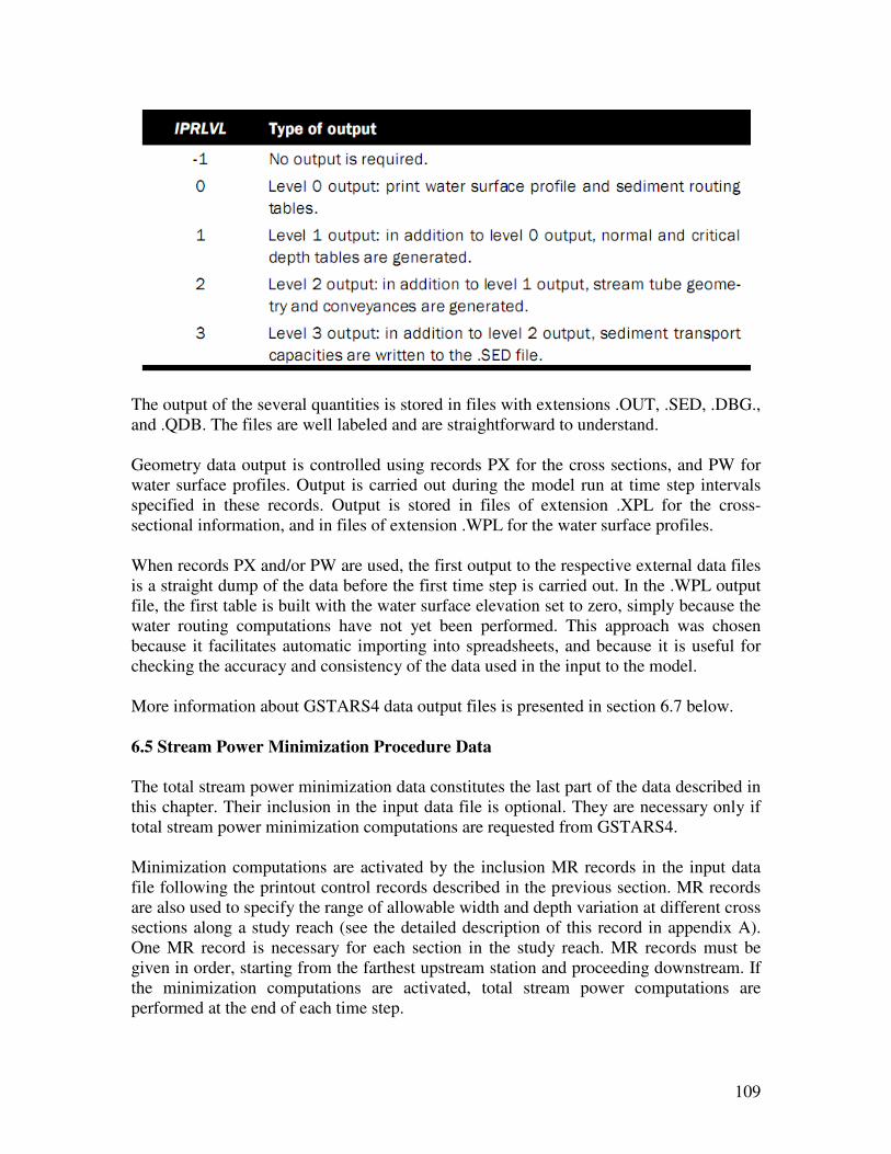
109
The output of the several quantities is stored in files with extensions .OUT, .SED, .DBG.,
and .QDB. The files are well labeled and are straightforward to understand.
Geometry data output is controlled using records PX for the cross sections, and PW for
water surface profiles. Output is carried out during the model run at time step intervals
specified in these records. Output is stored in files of extension .XPL for the cross-
sectional information, and in files of extension .WPL for the water surface profiles.
When records PX and/or PW are used, the first output to the respective external data files
is a straight dump of the data before the first time step is carried out. In the .WPL output
file, the first table is built with the water surface elevation set to zero, simply because the
water routing computations have not yet been performed. This approach was chosen
because it facilitates automatic importing into spreadsheets, and because it is useful for
checking the accuracy and consistency of the data used in the input to the model.
More information about GSTARS4 data output files is presented in section 6.7 below.
6.5 Stream Power Minimization Procedure Data
The total stream power minimization data constitutes the last part of the data described in
this chapter. Their inclusion in the input data file is optional. They are necessary only if
total stream power minimization computations are requested from GSTARS4.
Minimization computations are activated by the inclusion MR records in the input data
file following the printout control records described in the previous section. MR records
are also used to specify the range of allowable width and depth variation at different cross
sections along a study reach (see the detailed description of this record in appendix A).
One MR record is necessary for each section in the study reach. MR records must be
given in order, starting from the farthest upstream station and proceeding downstream. If
the minimization computations are activated, total stream power computations are
performed at the end of each time step.
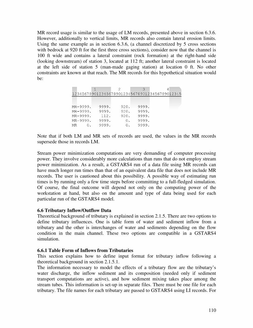
110
MR record usage is similar to the usage of LM records, presented above in section 6.3.6.
However, additionally to vertical limits, MR records also contain lateral erosion limits.
Using the same example as in section 6.3.6, (a channel discretized by 5 cross sections
with bedrock at 920 ft for the first three cross sections), consider now that the channel is
100 ft wide and contains a lateral constraint (rock formation) at the right-hand side
(looking downstream) of station 3, located at 112 ft; another lateral constraint is located
at the left side of station 5 (man-made gaging station) at location 0 ft. No other
constraints are known at that reach. The MR records for this hypothetical situation would
be:
Note that if both LM and MR sets of records are used, the values in the MR records
supersede those in records LM.
Stream power minimization computations are very demanding of computer processing
power. They involve considerably more calculations than runs that do not employ stream
power minimization. As a result, a GSTARS4 run of a data file using MR records can
have much longer run times than that of an equivalent data file that does not include MR
records. The user is cautioned about this possibility. A possible way of estimating run
times is by running only a few time steps before committing to a full-fledged simulation.
Of course, the final outcome will depend not only on the computing power of the
workstation at hand, but also on the amount and type of data being used for each
particular run of the GSTARS4 model.
6.6 Tributary Inflow/Outflow Data
Theoretical background of tributary is explained in section 2.1.5. There are two options to
define tributary influences. One is table form of water and sediment inflow from a
tributary and the other is interchanges of water and sediments depending on the flow
condition in the main channel. These two options are compatible in a GSTARS4
simulation.
6.6.1 Table Form of Inflows from Tributaries
This section explains how to define input format for tributary inflow following a
theoretical background in section 2.1.5.1.
The information necessary to model the effects of a tributary flow are the tributary’s
water discharge, the inflow sediment and its composition (needed only if sediment
transport computations are active), and how sediment mixing takes place among the
stream tubes. This information is set-up in separate files. There must be one file for each
tributary. The file names for each tributary are passed to GSTARS4 using LI records. For
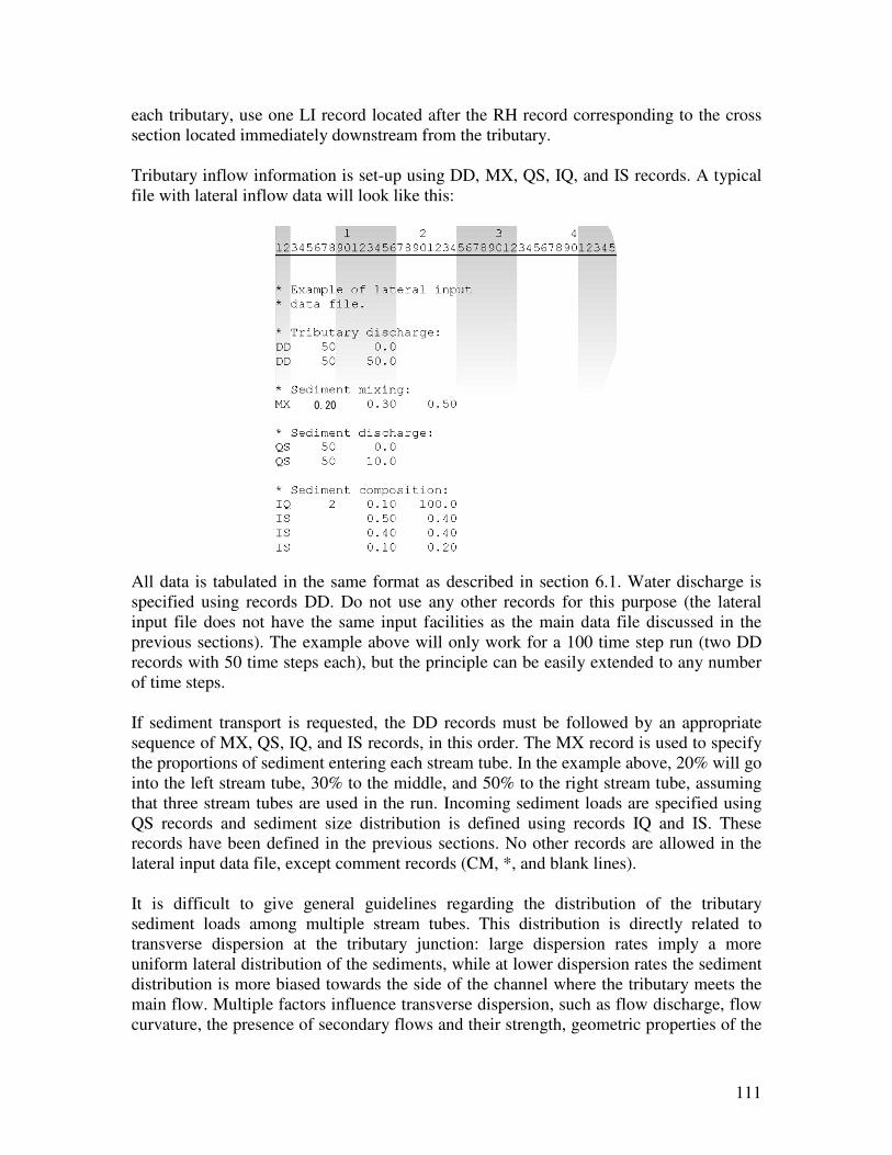
111
each tributary, use one LI record located after the RH record corresponding to the cross
section located immediately downstream from the tributary.
Tributary inflow information is set-up using DD, MX, QS, IQ, and IS records. A typical
file with lateral inflow data will look like this:
All data is tabulated in the same format as described in section 6.1. Water discharge is
specified using records DD. Do not use any other records for this purpose (the lateral
input file does not have the same input facilities as the main data file discussed in the
previous sections). The example above will only work for a 100 time step run (two DD
records with 50 time steps each), but the principle can be easily extended to any number
of time steps.
If sediment transport is requested, the DD records must be followed by an appropriate
sequence of MX, QS, IQ, and IS records, in this order. The MX record is used to specify
the proportions of sediment entering each stream tube. In the example above, 20% will go
into the left stream tube, 30% to the middle, and 50% to the right stream tube, assuming
that three stream tubes are used in the run. Incoming sediment loads are specified using
QS records and sediment size distribution is defined using records IQ and IS. These
records have been defined in the previous sections. No other records are allowed in the
lateral input data file, except comment records (CM, *, and blank lines).
It is difficult to give general guidelines regarding the distribution of the tributary
sediment loads among multiple stream tubes. This distribution is directly related to
transverse dispersion at the tributary junction: large dispersion rates imply a more
uniform lateral distribution of the sediments, while at lower dispersion rates the sediment
distribution is more biased towards the side of the channel where the tributary meets the
main flow. Multiple factors influence transverse dispersion, such as flow discharge, flow
curvature, the presence of secondary flows and their strength, geometric properties of the
0.20
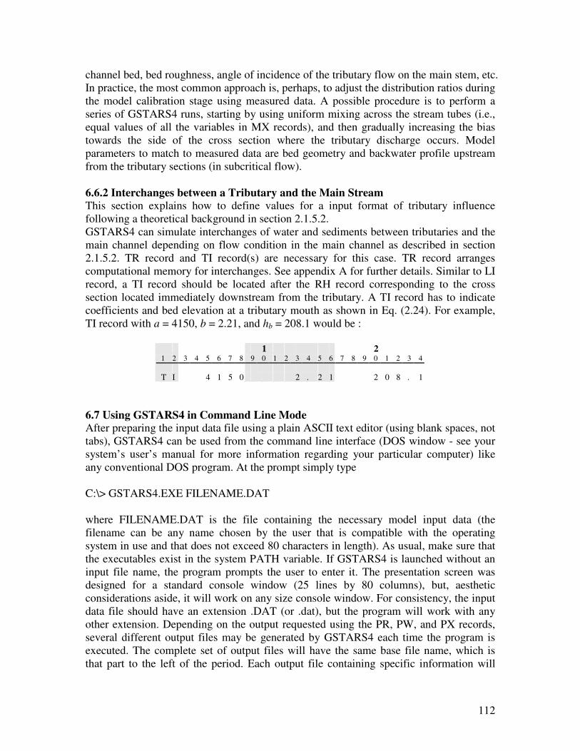
112
channel bed, bed roughness, angle of incidence of the tributary flow on the main stem, etc.
In practice, the most common approach is, perhaps, to adjust the distribution ratios during
the model calibration stage using measured data. A possible procedure is to perform a
series of GSTARS4 runs, starting by using uniform mixing across the stream tubes (i.e.,
equal values of all the variables in MX records), and then gradually increasing the bias
towards the side of the cross section where the tributary discharge occurs. Model
parameters to match to measured data are bed geometry and backwater profile upstream
from the tributary sections (in subcritical flow).
6.6.2 Interchanges between a Tributary and the Main Stream
This section explains how to define values for a input format of tributary influence
following a theoretical background in section 2.1.5.2.
GSTARS4 can simulate interchanges of water and sediments between tributaries and the
main channel depending on flow condition in the main channel as described in section
2.1.5.2. TR record and TI record(s) are necessary for this case. TR record arranges
computational memory for interchanges. See appendix A for further details. Similar to LI
record, a TI record should be located after the RH record corresponding to the cross
section located immediately downstream from the tributary. A TI record has to indicate
coefficients and bed elevation at a tributary mouth as shown in Eq. (2.24). For example,
TI record with a = 4150, b = 2.21, and hb = 208.1 would be :
1 2
1 2 3 4 5 6 7 8 9 0 1 2 3 4 5 6 7 8 9 0 1 2 3 4
T I 4 1 5 0 2 . 2 1 2 0 8 . 1
6.7 Using GSTARS4 in Command Line Mode
After preparing the input data file using a plain ASCII text editor (using blank spaces, not
tabs), GSTARS4 can be used from the command line interface (DOS window - see your
system’s user’s manual for more information regarding your particular computer) like
any conventional DOS program. At the prompt simply type
C:\> GSTARS4.EXE FILENAME.DAT
where FILENAME.DAT is the file containing the necessary model input data (the
filename can be any name chosen by the user that is compatible with the operating
system in use and that does not exceed 80 characters in length). As usual, make sure that
the executables exist in the system PATH variable. If GSTARS4 is launched without an
input file name, the program prompts the user to enter it. The presentation screen was
designed for a standard console window (25 lines by 80 columns), but, aesthetic
considerations aside, it will work on any size console window. For consistency, the input
data file should have an extension .DAT (or .dat), but the program will work with any
other extension. Depending on the output requested using the PR, PW, and PX records,
several different output files may be generated by GSTARS4 each time the program is
executed. The complete set of output files will have the same base file name, which is
that part to the left of the period. Each output file containing specific information will

113
have a unique file extension, as outlined below. Make sure that existing files do not
contain any of the following file extensions, because they will be overwritten by the
GSTARS4 program.
For a given input file named sample.dat, the following files may be generated.
sample.out: the .OUT file is the main output file containing the results from the model
run. This file contains information about the input data set, as well as hydraulic and
sediment transport information. The output level in this file is determined by record PR.
sample.xpl: The .XPL file contains the cross section data points, which can be imported
to any generic spreadsheet program. This file is generated only if requested by the PX
record.
sample.wpl: The .WPL file contains the water surface profile data points. A water
surface profile plot is created for each requested time step. Similarly to the .XPL file,
information in this file may be viewed/plotted using a generic spreadsheet program. This
file is generated only if requested by the PW record.
sample.dbg: The .DBG file contains information about the model run which can be
helpful in finding errors or anomalies in the model run. This information includes all
comment records included in the input data set as well as additional information about the
hydraulics and sediment calculations performed by the model. The output level in this file
is also determined by record PR.
sample.sed: The .SED file contains sediment carrying capacities for each stream tube at
each section for the requested time steps. It also contains actual sediment in transport and
bed sorting information for the time step. It is generated if level 3 output is selected on
the PR record.
sample.qdb: The .QDB file contains water and sediment passed through the downstream
boundary. For the convenience of further uses, gradation of sediment is also included.
Information from this file can be used as the upstream boundary condition for a
downstream routing.
As mentioned above, thalweg and stage output is done to the .WPL file in a tabular
format appropriate for use with any general purpose spreadsheet program. Its only
purpose is to facilitate plotting of the channel's longitudinal bed and stage profiles. The
same information is also supplied in the .OUT file. The first lines of the file contain the
date and time stamp of the run, as well as the title of the study, entered using TT records
in the input data file (in the .DAT file). The remainder of the file contains the output of
the program for the time steps specified in record PW (in the .DAT file).
For each time step of output, a three-column table is printed containing NSTA + 1 rows
(NSTA is the number of stations used in the study). The first row contains (from left to
right) the number of stations used in the study, the discharge for that time step, and the

114
time step number. The remaining rows contain (from left to right) the station coordinate,
thalweg, and stage for the time step. Note that the first set in the file corresponds to time
step zero, i.e., to the conditions defined before the run starts. Therefore, the discharge and
stages are not defined (they are printed to the file as zero values).
Cross-sectional geometry is output to file .XPL, also in a tabular format appropriate for
use in a spreadsheet program. The data in this file shows cross section evolution in time.
Output is made at given time steps, as specified in record PX (in the input .DAT file).
Similarly to the .WPL file, the first lines of the file contain the date/time stamp of the run
and the title of the study. Cross sectional geometry for the entire reach is dumped to the
file at each desired time step. For each time step of the output, the data is structured in the
following manner:
· the first line contains the number of stations used in the study (NSTA);
· data is grouped by station, starting at the station farthest upstream and ending at the
station farthest downstream;
· for each station, the first row of data contains three entries: location of station (as
defined in record ST, in the input .DAT file), the number of coordinate pairs used for that
station (NPTS); and the time step. The remaining rows contain NPTS pairs of coordinates,
with bed elevation in the first column and lateral coordinate in the second column.
The first set in the file corresponds to time step zero, i.e., to the initial conditions.
Due to the nature of the algorithms used in GSTARS4, the number of coordinate points
used to describe each cross section may vary with time. The lateral location of coordinate
points may also change, especially if minimization computations are performed. Care
must be exercised by the user when preparing the data for plotting using a generic
spreadsheet program.
6.8 Compatibility with Earlier Versions
GSTARS3 data files will run successfully in GSTARS4 without any change. Many of the
code and algorithms of GSTARS4 were rewritten in order to upgrade the performance of
the model. As a result, a GSTARS4 run using input data files from earlier versions may,
in general, produce slightly different but similar results from those of earlier versions.
115
REFERENCES
Ackers, P., and White, W.R. (1973). "Sediment transport: new approach and analysis," J.
of the Hydr. Div. ASCE, 99(HY11).
Alonso, C.V. (1980). “Selecting a formula to estimate sediment transport capacity in
nonvegetated channels,” CREAMS (A Field Scale Model for Chemicals, Runoff,
and Erosion from Agricultural Management System), ed. by W.G. Knisel, U.S.
Department of Agriculture, Conservation Research Report no. 26, chap 5, pp.
426-439.
Alonso, C.V., Neibling, W.H., and Foster, G.R. (1982). “Estimating sediment transport
capacity in watershed modeling,” Trans. of the ASAE, 25( 5), pp. 1211-1220 and
1226.
Anderson, D.A., Tannehill, J.C., and Pletcher, R.H. (1997). Computational fluid
mechanics and heat transfer. 2nd ed. Taylor and Francis.
Arcement, G.J., and Schneider, V.R. (1987). Roughness coefficients for densely vegetated
flood plains. U.S. Geological Survey Water-Resources Investigation Report 83-
4247.
Ariathurai, R., and Krone, R.B. (1976). "Finite element model for cohesive sediment
transport," J. of the Hydr. Div. ASCE, 102(HY3).
ASCE Task Committee on Preparation of Sedimentation Manual, (1971). “Sedimen
transportation mechanics: H. Sediment discharge formulas,” J. of the Hydr. Div.
ASCE, 97(HY4).
ASCE (1982). “Relationships between morphology of small streams and sediment
yields,” by the ASCE Task Committee o Relations between Morphology of Small
Streams and Sediment Yield of the Committee on Sedimentation of the
Hydraulics Division, J. of the Hydr. Div. ASCE, 108( HY11), pp. 1328-1365.
Ashida, K., and Michiue, M. (1970). “Study on suspended sediment (1),” Annals DPRI,
No. 13B, pp. 233-242. (In Japanese.)
Ashida, K., and Michiue, M. (1972). “Study on hydraulic resistance and bed load
transport rate in alluvial streams,” Proc. JSCE, pp. 59-69. (In Japanese.)
Barnes, H.H. (1967). Roughness characteristics of natural channels. U.S. Geological
Survey Water-Supply Paper 1849.
Bennett, J.P., and Nordin, C.F. (1977). "Simulation of sediment transport and armoring,"
Hydrological Sciences Bulletin, XXII.
Chang, H.H. (1979). "Minimum stream power and river channel patterns," J. of
Hydrology, 41.
Chang, H.H. (1980a). "Stable alluvial canal design," J. of the Hydr. Div. ASCE,
106(HY5).
Chang, H.H. (1980b). "Geometry of gravel streams," J. of the Hydr. Div. ASCE,
106(HY9).
Chang, H.H. (1982a). "Mathematical model for erodible channels," J. of the Hydr. Div.
ASCE, 108(HY5).
Chang, H.H. (1982b). "Fluvial hydraulics of deltas and alluvial fans," J. of the Hydr. Div.
ASCE, 108(HY11).
Chang, H.H. (1983). "Energy expenditure in curved open channels," J. of the Hydr. Div.
ASCE, 109(HY7).

116
Chang, H.H., and Hill, J.C. (1976). "Computer modeling of erodible flood channels and
deltas," J. of the Hydr. Div. ASCE, 102(HY10).
Chang, H.H., and Hill, J.C. (1977). "Minimum stream power for rivers and deltas," J. of
the Hydr. Div. ASCE, 103(HY12).
Chang, H.H., and Hill, J.C. (1982). "Modeling river-channel changes using energy
approach," Proc. of the ASCE Hydraulics Division Conference on Applying
Research to Hydraulic Practice, Peter E. Smith (ed.).
Chow, V.T. (1959). Open-channel hydraulics. McGraw-Hill, New York, NY.
Colby, B.R., (1963). Discussion of "Sediment transport mechanics: introduction and
properties of sediment," J. of the Hydr. Div. ASCE, 89(HY1).
Cowan, W.L. (1956). “Estimating hydraulic roughness coefficients,” Agricultural
Engineering 37, July, pp. 473-475.
Cunge, J.A., Holly, F.M., and Verwey, A. (1980). Practical aspects of computational
river hydraulics. Pitman Publishing, Inc., Marshfield, MA.
DuBoys, M.P. (1879). “Le Rhône et les rivières à lit affouillable,” Annals de Ponts et
Chaussée, 18(5), pp. 141-195. (In French.)
Egiazaroff, I.V. (1965). “Calculation of nonuniform sediment concentration,” J. of the
Hydr. Div. ASCE, 91(HY4), pp. 225-246.
Einstein, H.A. (1950). The bed-load function for sediment transportation in open channel
flows. U.S. Department of Agriculture, Soil Conservation Service, Technical
Bulletin No. 1026.
Einstein, H.A., and Chien, N. (1953). Transport of sediment mixtures with large range of
grain size. University of California Institute of Engineering Research, Missouri
River Division Sediment Series, No. 2.
Engelund, F., and Hansen, E. (1972). A monograph on sediment transport in alluvial
streams. Teknish Forlag, Technical Press, Copenhagen, Denmark.
French, R.H. (1985). Open-channel hydraulics. McGraw-Hill Book Company, New York,
NY.
Gomez, B., and Church, M. (1989). “An assessment of bed load sediment transport
formulae for gravel bed rivers,” Water Resources Research, 25(6), pp. 1161-1186.
Han, Q. (1980). "A study on the non-equilibrium transportation of suspended load,” Proc.
of the Int. Symposium on River Sedimentation, Beijing, China, pp. 793-802.
(InChinese.)
Han, Q., and He, M. (1990). "A mathematical model for reservoir sedimentation and
fluvial processes," Int. J. of Sediment Res., 5(2), IRTCES, pp. 43-84.
Henderson, F.M. (1966). Open channel flow. MacMillan Book Company, New York, NY.
Hirsch, C. (1988). Numerical computation of internal and external flows. 2 vols. John
Wiley & Sons, Inc.
HR Wallingford (1990). Sediment transport, the Ackers and White theory revised. Report
SR237, HR Wallingford, England.
Huang, J. V., and Greimann B. (2007) User’s Manual for SRH-1D V2.0 (Sedimentation
and River Hydraulics – One Dimension, Version 2.0). Technical Service Center,
U.S. Bureau of Reclamation, Denver, Colorado.
Ikeda, S., Yamasaka, M., and Chiyoda, M. (1987). “Bed topography and sorting in
bends,” J. of Hydr. Engng., ASCE, 113(2), pp. 190-206.
117
IRTCES (1985). Lecture notes of the training course on reservoir sedimentation.
International Research and Training Center on Erosion and Sedimentation,
Sediment Research Laboratory of Tsinghua University, Beijing, China.
Kikkawa, M., Ikeda, S., and Kitagawa, A. (1976). "Flow and bed topography in curved
open channels," J. of the Hydr. Div. ASCE, 102(HY9), pp. 1327-1342.
Klaassen, G., Ogink, H., and van Rijn, L. (1986). “DHL-Research on bedforms,
resistance to flow and sediment transport,” 3rd Int. Symp. on River Sedimentation,
Jackson, MS, pp. 58-82.
Krone, R. B. (1962). Flume studies of the transport of sediment in estuarial processes.
Hydraulic Engineering Laboratory and Sanitary Engineering Research Laboratory,
University of California, Berkeley, CA.
Lane, E. W. (1947). “Report of the subcommittee on sediment terminology,” Trans.,
Amer. Geophys. Union, 28(6), Washington, D.C.
Laurenson, E.M. (1986). “Friction slope averaging in backwater calculations,” J. Hydr.
Engng., ASCE, 112(2), pp. 1151-1163.
Laursen, E.M.(1958). "The total sediment load of streams," J. of the Hydr. Div. ASCE,
84(HY1).
Lewis, T.M. (1996). Reservoir sedimentation code extensions for the GSTARS2 computer
model, Internal Report, Golder and Associates, Inc., Lakewood, CO.
Lyn, D. A. (1987). “Unsteady sediment-transport modeling,” J. Hydr. Engng., ASCE,
113(1), pp. 1-15.
Madden, E., (1993). Modified Laursen method for estimating bed-material sediment load,
USACE-WES, Contract Report HL-93-3.
Mehta, A. J., Hayter, E. J., Parker, W. R., Krone, R. B., and Teeter, A. M. (1989).
“Cohesive sediment transport I: Processes description,” J. Hydr. Engng., ASCE,
115(8), pp. 1076-1093.
Meyer-Peter, E., and Müller, R. (1948). "Formula for bed-load transport," Proc. of the Int.
Assoc. for Hydraulic Research, 2nd Meeting, Stockholm.
Molinas, A., and Yang, C.T. (1985). "Generalized water surface profile computations," J.
of the Hydr. Div. ASCE, 111(HY3).
Ohtsubo, K., and Muraoka, K. (1986). “Resuspension of cohesive sediments by currents,”
3rd Int. Symp. on River Sedmentation, Jackson, MS, pp. 1680-1689.
Parker, G. (1990). "Surface based bedload transport relationship for gravel rivers," J. of
Hydr. Res., 28(4), pp. 417-436.
Partheniades, E. (1965). "Erosion and deposition of cohesive soils." J. of the Hydr. Div.
ASCE, 91(HY1).
Partheniades, E. (1986). “The present state of knowledge and needs for future research on
cohesive sediment dynamics,” 3rd Int. Symp. on River Sedimentation, Jackson,
MS, pp. 3-25.
Reed, J.R., and Wolfkill, A.J. (1976). "Evaluation of friction slope models," Rivers'76
Symposium on Inland Waterways for Navigation, Flood Control, and Water
Diversions Colorado State University, Ft. Collins.
Rubey, W. (1933). "Settling velocities of gravel, sand, and silt particles," Am. J. of
Science, 25.
Samuels, P.G. (1990). “Cross-section location in 1-D models,” Int. Conf. on River
Hydraulics, ed. by W. White, John Wiley & Sons, pp. 339-350.

118
Song, C.C.S., and Yang, C.T. (1979a). "Velocity profiles and minimum stream power," J.
of the Hydr. Div. ASCE, 105(HY8).
Song, C.C.S., and Yang, C.T. (1979b). "Minimum stream power: theory," J. of the Hydr.
Div. ASCE, 105(HY8).
Song, C.C.S., and Yang, C.T. (1982a). "Application of variation principle to river flow,"
Applying Research to Hydraulic Practice, ASCE, Peter E. Smith (ed.).
Song, C.C.S., and Yang, C.T. (1982b). "Minimum energy and energy dissipation rate," J.
of the Hydr. Div. ASCE, 108(HY5).
Straub, L.G. (1935). Missouri River report. In-House Document 238, 73rd Congress, 2nd
Session, U.S. Government Printing Office, Washington, D.C.
Toffaleti, F.B. (1968). "Definitive computations of sand discharge in rivers," J. of the
Hydr. Div. ASCE, 95(HY1).
U.S. Army Corps of Engineers (1993). The Hydraulic Engineering Center, HEC-6 Scour
and Deposition in Rivers and Reservoirs, User's Manual. Mar. 1977 (revised
1993).
U.S. Interagency Committee on Water Resources, Subcommittee on Sedimentation
(1957). Some fundamentals of particle size analysis, Report no. 12.
van Rijn, L.C. (1984). “Sediment transport, part III: alluvial roughness,” J. Hydr. Engng.,
ASCE, 110(12).
Vetter, M. (1987). Der Transport suspendierter Feststoffe in offenen Gerinnen,
Mitteilungen Institut für Wasserwesen, University of the German Federal Army,
Report no. 19. (In German.)
Vetter, M. (1988). Gesamttransport von Sedimenten in offenen Gerinnen, Mitteilungen
Institut für Wasserwesen, University of the German Federal Army, Report no. 26.
(In German; translated to English by the U.S. Bureau of Reclamation, May 1989.)
Vries, M. de (1969). Solving river problems by hydraulic and mathematical models. Delft
Hydraulics Laboratory Publication 76-II.
Waananen, A.O., Harris, D.D., and Williams, R.C. (1971). Floods of December 1964 and
January 1965 in the far Western United States: Part 1, Description.U.S.
Geological Survey Water-Supply Paper 1866-A.
White, W.R., Milli, H., and Crabbe, A.D. (1975). “Sediment transport theories: review,”
Proc. of the Inst. of Civil Engineers, 59(2), pp. 265-292.
Yang, C.T. (1971). "Potential energy and stream morphology," Water Resources
Research, AGU, 7(2), pp. 311-322.
Yang, C.T. (1973). "Incipient motion and sediment transport," J. of the Hydr. Div. ASCE,
99(HY10), pp. 1679-1704.
Yang, C.T. (1976). "Minimum unit stream power and fluvial hydraulics," J. of the Hydr.
Div. ASCE, 102(HY7), pp. 919-934.
Yang, C.T. (1979). "Unit stream power equations for total load," J. of Hydrology, 40.
Yang, C.T. (1984). "Unit stream power equation for gravel," J. of the Hydr. Div. ASCE,
110(HY12), pp. 1783-1797.
Yang, C.T. (1992). "Force, energy, entropy, and energy dissipation rate," Entropy and
Energy Dissipation in Water Resources, V.P. Sing and M. Fiorentino (eds.),
Kluwer Academic Publisher, Netherlands.
Yang, C.T. (1996). Sediment transport: theory and practice. McGraw-Hill Companies,
Inc., New York, NY. (Reprinted by Krieger Publishing Company, 2003.)
119
Yang, C. T. (2003). Sediment transport theory and practice. Krieger Publishing
Company, Malabar, FL.
Yang, C.T., and Song, C.C.S. (1979). "Theory of minimum rate of energy dissipation," J.
of the Hydr. Div. ASCE, 105(HY7), pp. 769-784.
Yang, C.T., and Song, C.C.S. (1986). "Theory of minimum energy and energy dissipation
rate," Encyclopedia of Fluid Mechanics, Vol. 1, Chapter 11, Gulf Publishing
Company, N.P. Cheremisinoff (ed.), pp. 353-399.
Yang, C.T., and Wan, S. (1991). “Comparisons of selected bed material load formulas,” J.
of Hydr. Engng., ASCE, 117(8), pp. 973-989.
Yang, C.T., Molinas, A., and Wu, B. (1996). "Sediment transport in the Yellow River," J.
of Hydr. Engng., ASCE, 122(5).
Yang, C.T., Trevino, M.A., and Simoes, F.J.M. (1998). User’s manual for GSTARS 2.0
(Generalized Stream Tube model for Alluvial River Simulation version 2.0). U.S.
Bureau of Reclamation, Technical Service Center, Denver, CO.
Yang, C.T. and Simões, F.J.M. (2000). User’s manual for GSTARS 2.1 (Generalized
Stream Tube model for Alluvial River Simulation version 2.1). U.S. Bureau of
Reclamation, Technical Service Center, Denver, CO.
Yang, C.T., and Huang, C. (2001). “Applicbility of sediment transport formulas,” Int. J.
of Sediment Res. 16(3), pp. 335-353.
Yang, C. T., and Somões, F. J. M. (2002). User’s Manual for GSTARS3 (Generalized
Sediment Transport model for Alluvial River Simulation version 3.0), U.S. Bureau
of Reclamation, Technical Service Center, Denver, CO.
Yang, C. T., Huang, J. V., and Greimann, B. P. (2004). User’s Manual for GSTAR-1D
1.0 (Generalized Sediment Transport for Alluvial Rivers – One Dimension,
Version 1.0, U.S. Bureau of Reclamation, Denver, CO.