The NSE-Government Securities Index: Issues in construction

Vardhana Pawaskar1, Sudipta Dutta Roy, Gangadhar Darbha

National Stock Exchange Of India Ltd Exchange Plaza, Bandra (East), Mumbai – 400 051

phone: (022) 659 8291 Fax (022) 659 8288

September 2002

Abstract The increased activity in the government securities market in India and

simultaneous emergence of mutual (gilt) funds has given rise to the need for a well-

defined Bond Index to measure returns in the bond market. The NSE-Government

Securities Index prices components off the NSE Benchmark-ZCYC, so that movements

reflect returns to an investor on account of change in interest rates only, and not those

arising on account of the impact of idiosyncratic factors. The index is available from

January 1. 1997 to the present. The index would provide a benchmark for portfolio

management by various investment managers and gilt funds. It could also form the

basis for designing index funds and for derivative products such as options and futures.

Keywords: Bond index, Benchmark, Index Funds

1 Corresponding author e-mail: vpawaskar@nse.co.in

1. Introduction

The government securities market in India has seen a significant increase in the

volume of secondary market trading by banks, financial institutions and mutual funds.

The consolidated data from the RBI-SGL shows an average annual growth rate of over 96

per cent in secondary market volumes over the period 1994-95 to 2001-02.

Simultaneously, the emergence of mutual (gilt) funds as an avenue for investors to park

their investible funds has given rise to the need for a well-defined Bond Index to

compare returns in the bond market vis-à-vis the equity market. A well-defined and

widely accepted Government securities index would provide a benchmark for portfolio

management by various investment managers and gilt funds. The index could be used

by the fund managers to compare their fund vis-à-vis a benchmark, and by the investors

to judge and objectively choose between alternative debt funds. It could also form the

basis for derivative products such as options and futures.

In the present paper, we discuss and examine the various aspects of the

construction of the NSE – Government Securities Index. In section 2, we discuss the

issues in constructing a bond index and how they are different from those in the equity

context. Section 3 describes the existing Indian bond market indices and in section 4 we

describe the considerations used in NSE-GSI. Section 5, 6, 7 give the sub-indices, the

statistics that are used to describe the index portfolio and the formulae for the index. In

section 8, we discuss briefly how the index could be used specifically to design an Index

fund. Section 9 describes the movement of the NSE – GSI over the period from Jan ’01 to

Jun ’02. Finally section 10 concludes and section 11 gives the scope for further work in

refinement of the index.

2. Issues in constructing an index for the bond markets

Analogous to the construction of an equity index, the issues in the construction

of a bond index relate to (i) the specification of a selection criterion to decide which

bonds form part of the index and (ii) the prices to be used to compute the index.

However, the actual implementation of the basic principles is rendered different on

account of certain inherent factors that distinguish the two types of instruments. Unlike

equity, new bonds are issued at frequent intervals and existing bonds redeem, so that

the universe of bonds changes continuously. This makes it difficult to hold the index

composition constant over a considerable period of time, unlike in an equity index whose

constituents remain unchanged over long periods of time. Further, the secondary

market for bonds is significantly less liquid than the equity market. In addition, the

liquidity of individual bonds fluctuates over its life cycle. Together, these have the

following implications. First, the index composition would have to be changed frequently

even with selection criteria that incorporate a measure of liquidity. Secondly, irrespective

of the selection criterion used to identify the securities that go into the index, it may not

be possible to observe market prices for all of them on a daily basis.

Any index should reflect the movement of the fundamental factors that affect the

market. In the equity market, for instance, the index reflects the fundamental factors

that affect the economy/stock market as a whole, with (random) individual stock specific

news getting canceled out by averaging. By contrast, several empirical studies have

demonstrated that the liquidity / illiquidity premia associated with bonds can be traced

to their individual attributes like outstanding issue amounts, time since issuance and

time to maturity and are, to that extent, systematic in nature. While this systematic

component may be removed by averaging over a sufficiently diversified index

composition, market prices, as already mentioned, may not be available for all the

constituents of such an index. This issue assumes greater significance in the Indian

market where only a handful of all outstanding Government securities witness trading at

any point of time.

While market prices may not be available for all the index constituents on a daily

basis, we do, however, have well-defined methodologies to isolate the common factor, the

term structure of interest rates, from other security specific idiosyncratic factors. If we

have an estimate of the term structure prevailing on any day, it is possible to arrive at

prices of all outstanding bonds - even if some of them are not traded on a particular day

- on the basis of the available estimate of the term structure. These prices reflect the

price predicted by the underlying term structure - the common factor - alone, and can

be used as representative prices for computing the bond index.

3. Existing market indices for the Indian Bond Market

The bond market indices available for the Indian Government Securities market

are IBEX published by ICICI Securities, J.P.Morgan’s India Government Bond Index

(JPM-IGBI), the SBI-Gilt Index. Table 1 lists the methodology used in constructions of

these indices. The two main factors are the selection criteria used to include bonds in

the index and secondly the prices used to value these securities.

The price used is the market price whenever available or the last traded price

(other than for the GILT index which uses model prices). The market prices (even for the

most liquid securities) may not be available on a daily basis. In such cases the

indices use the last traded price of the security. The last traded price reflects a price that

relates the daily term structure prevailing on the day on which a trade(s) occurred which

may/may not be the same as on the day the index value is being calculated. A related

issue is that it might involve use of LTPs on different dates for different bonds. Thus

using the last traded price has its own problems.

In a marked departure from the existing indices outlined above which use market

prices, Thomas and Shah (2000) propose use of ZCYC based prices for the construction

of a bond index (the NSE-ZCYC based Government Bond Index). The strength of this

approach lies in the fact that all prices used relate to the term structure of a particular

day, unlike LTPs that are used for the other indices. Further, availability of model-based

prices for all outstanding securities on a daily basis allows independent treatment of

“pricing” and “selection criterion” in designing a bond index.

The selection criteria for all the indices is such that the securities in the index

portfolio are the most liquid securities existing in the market. The liquid securities are

determined on the basis of observed outcome (number of trade /volume).

These indices use market capitalization based weights to give higher weightage to

bonds with higher amounts outstanding. Subramanian (2000) argues that such weights

are not proxy for higher liquidity in the security. Unlike in capital markets where greater

market capitalization is associated with securities with higher liquidity and the theory of

efficient markets holds good, the same implication does not hold in the bond markets.

However in bond markets capital flows to the ‘more’ liquid securities which have easy

replicability and hence lower transactions costs. The author argues for a relative

liquidity function based weights that depend on the traded amount, the number of

trades and the number of days when the security traded.

To formulate selection criterion or liquidity weights based on the observed

outcome in terms of various factors of the trade in the security could lead to serious

problems. Liquidity or liquidity weights here have not been determined by the structural

features of the security, such as age (time since issue), time to maturity, coupon and

issue size. Trade specific categorization of the securities as liquid/illiquid would be

based on certain subjective judgment. In the Indian context, it has been shown that

information from the observed trade(s), like trade volume/number of trades, does not

proxy for liquidity of a security (Darbha, Dutta Roy and Pawaskar, 2002).

4. Construction of the NSE-GSI

A Standing commission of the EFFAS and ISMA formed a committee to discuss

and examine the various aspects of construction of bond indices (Brown, 1994). They

have proposed a set of rules for indices that could be directly applied over different

domestic markets. In what follows, the suggestions from the report and other

assumptions used in the construction of the NSE-GSI are discussed.

4.1 Portfolio emulation

For an index to reflect changes in the underlying portfolio, it has to be

constructed such that its constituents are held in the same proportions as in the index.

Ignoring the presence of any cashflows, if the total value of the underlying investments

in an index rises by 50 percent, then the value of the index should also rise by 50

percent. The index so computed is based on arithmetic and not geometric calculations.

The basic principle used in the geometric calculation is to multiply the prices of all the n

constituents together, take the nth root and then multiply by a factor to produce the

index. When the constituents of the index are changed, the factor is adjusted, so that

there is no discontinuity in the values. Although this approach is reasonably good at

reflecting price movements over a short time period, it can be shown that it does not

reflect the performance of a portfolio. In the arithmetic calculations, the index is taken

as the weighted average value of the portfolio the weights being the size of the holdings.

[Insert Example 1 here].

4.2. Weighting scheme

In most indices, each individual security is weighted by either its outstanding

market value or by its outstanding par value. Both market value and par value

weightings are designed to give large issues a greater role in the total return of an index.

Such weighting in the fixed income market is, in fact, a vestige of capital market theory

which suggests that in the equity market, individual stocks in an efficient portfolio

should be weighted by their capitalization. There are some indices in which all the

securities receive equal weighting. Such weighting scheme is simple and does not make

any assumptions about the extent of liquidity of one security against the other.

Subramanian (2001) suggests liquidity based weighting scheme as an alternative to

market capitalization based weights. However, for reasons mentioned earlier, we do not

believe that weights created simply off the trade measures could reflect liquidity in a

consistent manner. For the NSE-GSI we still use the market capitalization based

weights, inasmuch as large market values imply greater liquidity of securities in the

secondary market and small par values imply lesser liquidity. Darbha, Dutta Roy and

Pawaskar (2002) study indicates issue size outstanding as an important indicator of

liquidity.

4.3. Selection criteria

All outstanding sovereign securities (the Treasury Bills and dated government securities)

are used to generate the NSE-GSI. The index, however, does not include bonds with

additional features such as the floating rate bonds and the indexed bonds.

4.4. Pricing

The bond market indices can be constructed using either the daily market prices,

the last traded price or the estimated model prices. The daily market prices may/may

not be available on a consistent basis for all securities in the index. Secondly, these

prices take into account the effect due to interest rates and also the security specific

premia, that could vary between securities and also between trades. The problem with

last traded prices has been discussed earlier.

A unique feature of bond prices is the separability of the fundamental factors

viz., the interest rates from the security specific factors. Daily trades information can be

used to determine the fundamental factors that drive bond pricing, the term structure of

interest rates, also called as the zero coupon yield curve (ZCYC). The term structure of

interest rates gives the spot rates for any maturity value. With the ZCYC for any day

available, non-traded bonds can be priced given their security features such as coupon

and time to coupon/redemption.

For the NSE-GSI, we use prices that are estimated off the “benchmark term

structure of interest rates” (Darbha, 2002). This differs from the average ZCYC based

pricing proposed by Thomas and Shah (2000). If the bond index is to reflect daily

changes in interest rates alone, the term structure used for pricing should ideally reflect

'benchmark' rates, purged of liquidity effects. Such rates are obtained from the NSE-

benchmark yield curve which uses the frontier function approach to estimate the daily

term structure of sovereign rates. The benchmark ZCYC is estimated after controlling for

the security specific factors and the price off this benchmark yield curve reflects the

shadow price that the security would command if it was as liquid as the most-liquid

security in the portfolio.

4.5. Portfolio rebalancing

The index constructed should have the ability to add new issues and also have

the provision to remove old issues when redeemed. Any change in the outstanding

amount of a bond issue due to re-issue has to be accounted. Such changes in the

constituents, while the prices are unchanged should not cause the index calculations to

jump. A chain-linked calculation method adequately solves this problem, i.e., today's

index value is defined to be the previous calculation times the aggregate percentage

change in the value of the current constituents since the previous calculation. [Insert

Example 2 here]

The chain-link method must be adapted to allow the constituent bonds to change

their issue size. Change in issue-size can occur when there is a re-issue which is

fungible with it (i.e. it has the same cash flow structure as the original issue). The

change adaptation is achieved by weighting both the current and previous prices by the

amount in issue at the previous date. [Insert example 3 here]

The chain-linked formula allows for any change in weights attached to each

bond, and also to add and subtract bonds at any time. If a bond is redeemed, or drops

from the index for any reason, the formula in effect reinvests the proceeds in all the

other bonds in the index in proportion to their sizes. For a new issue, the opposite

process occurs. The weights associated with the constituent bonds are usually adjusted

on the day they take effect. Indices using the chain-link process can be calculated with

any desired frequency. The issues have to be included in the index as soon as they

become available for trading which is usually the next day after the allotment.

4.6. Reinvestment assumption

Although, as has been discussed, the constituents of an index group normally

remain unchanged during each selection period (it could be daily, monthly or even

longer period), they normally create intermediate cashflows in the form of coupon

payments and redemptions. Conversely, they may absorb cashflows when a new issue is

added. Receipts from coupon payments are ignored when calculating the clean price

index, although redemptions etc., still need to be accounted for. The question then

arises as to how one should invest these cashflows. For the purpose of the discussion, it

is assumed that cashflows are only created. Various options are possible:

1) Remove the proceeds from the calculation.

2) Put the proceeds into an included ‘cash’ stock which does not earn any interest.

3) Put the proceeds into an included ‘cash’ stock which earns interest at an appropriate

rate.

4) In the case of a coupon payment, for the total return index, reinvest the proceeds

ignoring any transaction costs in the security that produced the cashflow. A different

procedure is obviously required for the final redemption of a security.

5) Reinvest the proceeds in the index constituents according to their weights. All

theoretical transactions costs are ignored.

The first option is satisfactory if the objective is to calculate an index which

measures the capital performance, while ignoring any income. It is thus not the basis for

a total return index, although it could be used for a clean price index if allowances are

made for changes in constituents.

The second option is unsatisfactory since, over time, the cash element could become

large, although it could be reinvested at the beginning of the next period when the

constituent bonds are reviewed. This would have the effect of dampening the index

movements, and does not reflect any return on this money. Such an index would

perform better than the market in a bear market, and worse in a bull market.

The third option, although an improvement on the second, means that an external

rate of interest has to be chosen - and specified. Is this an over-night, monthly, or even

3-month rate? This is contrary to the basic principle that external factors should not

affect the performance of an index group. Another approach would be to assume that the

cash accrues interest at the average coupon rate of the index. This again has its

limitations since such returns may not be realizable.

The fourth option - whereby coupons are reinvested in the security which produced

the cashflow - has limitations, since the performance of the index would now be

dependent on the base date of the index. [Insert Example 4 here]. Another problem

associated with this approach is that, over time, securities with high coupons will get

disproportionately large weightings compared with zero- or low-coupon bonds.

The fifth option-of reinvesting the proceeds in the index in the proportion to the

size of the holdings has none of the problems associated with the other alternatives.

However, it does have the disadvantage that it is frequently not possible to implement in

practice, even if all transactions costs are ignored, since one cannot purchase part of a

bond. This objection does not invalidate the mathematics and, as a result, it is this

option which is used in creation of the NSE-GSI. [Insert Example 5 here]

4.7. Reviewing the index portfolio

In case of most of the indices the basket of the bonds included is reviewed on a

monthly frequency. During the month the daily indices are computed using the same

basket of bonds. New issues are not included immediately in the portfolio as their price

is said to be volatile and would contain noise. New issues during the month and the

redemptions during the month are all updated for the index portfolio only at the

beginning of the next month. The question is whether such long time period between the

market portfolio and the index portfolio (as in the case of index using all outstanding

bonds) makes the index reflective of the current market position.

The closest alternative to current market position is the option to review the

basket of bonds daily. It becomes a major issue when the case is, as in few markets, that

new issues may not be available to the market for trading until quite some time. In the

Indian Bond Market, the bonds are available for trading from the next day of the issue.

Hence having daily updation of the bond index is not impossible to achieve.

4.8. Frequency of calculation and treatment of non-working days

To account for new issues, re-issues and redemptions the indices are calculated

on daily basis. The weekends and holidays are ignored. If a payment falls due on a

weekend or bank holiday, then it is normal for the payment not to be received until the

next business day, with the result that any monies cannot be reinvested in the index

until then. The chain-link nature of the index means that it will allow for this if it is only

calculated on business days. An index on a weekend or bank holiday is, by convention,

assumed to be the same as that on the previous business day, although interest does

continue to accrue.

Coupons and redemption amounts are credited directly to participants current

accounts held with the RBI. When the date of redemption of a T-Bill falls on a holiday,

the holder receives the redemption amount on the previous business day. When the date

of coupon payment or redemption for a dated Government security falls on a holiday, the

amounts are paid out on the following business day. For the purpose of the NSE- GSI we

assume that all cashflows that fall on holidays are reinvested on the next working day.

5. Sub-indices

It is recognized that there are various users of bond indices with each having

different requirements. For example, the long-term investors, have a portfolio that would

tend to encompass both liquid and illiquid bonds – and would require an index that

covers all the sectors and therefore appreciate an ‘All-bond’ or composite index. Active

fund managers on the other hand, are often more interested in the most liquid bonds in

a sector. The investment objectives for a tax-free pension fund are somewhat different to

those of a money market fund, and hence the type of securities in which they invest

would be different. Given the differing objectives, it is not sufficient to calculate just one

index for a market and assume that everyone can compare themselves against it. The

categories of sub-indices that have be provided are given below.

5.1 Security type sub-groups

The government securities market trades various securities, like the treasury

bills, dated government securities, index-linked bonds, floating rate securities etc. As of

now, the pricing technology available with us (NSE-Benchmark ZCYC) is robust in

pricing the treasury bills and the dated government securities and these form the two

security-wise categories for the sub-indices.

5.2 Time to Maturity sub-groups

It is not particularly useful for a portfolio manager to compare his performance

with an index, which has a much shorter or long time horizon than his portfolio, pension

funds, for example, often have a long-term horizon. As a result, it is considered desirable

to calculate indices for bonds with similar maturity expectations, in addition to the total

market calculations. Based on the residual time to maturity of the security the indices

are computed for the following sub-groups:

1) Bonds with residual maturity of 1-3 years (short - term)

2) Bonds with residual maturity of 3 - 8 years (medium – term)

3) Bonds with residual maturity over 8 years (long-term)

6. Descriptive Statistics for the index portfolio

The fixed income index funds cannot in principal purchase and hold all

securities in the same proportion as held in the index. The design of the index funds,

selects a basket of securities, whose aggregated profile characteristics (such as portfolio

yield, effective duration, and convexity) and expected total return match those of the

index. The objective is to minimize the difference between realized return from the index

fund and the return from the index. This difference also called the tracking error can in

principal never be completely eliminated.

6.1 Yield to maturity

The yield to maturity of a portfolio is the most simple and easily understood

measure. It gives the internal rate of return of holding the portfolio until maturity. In

computation, the portfolio is treated as a single entity. The cashflows from all its

constituent securities are weighted by the outstanding issue size and discounted at the

same rate, which is the YTM. A point to be mentioned is that YTM is security specific,

i.e., it’s value depends on the constituents of the portfolio, their coupon values. This

should not be confused with the interest rates as given from ZCYC which depend only on

the time to maturity and are not instrument specific.

6.2 Macaulay Duration

The concept of duration takes into account both the coupon and the redemption

payments and is sometimes taken as an alternative to the time to maturity measure.

Duration is defined as the average life of the present values of all future cashflows from

the bond. [Insert Example 6 here]. In calculating the present value of the future

cashflows, a discount rate equal to the redemption yield of the bond is used. The

duration B of a bond is given by:

∑

∑

=

== n

i

tii

n

i

tiii

CF

tCFD

1

1

*

**

υ

υ

where, n number of future coupons and capital cashflows

CFi , ith future cashflow

ti time in years to the ith cashflow

ν the annualized discounting factor

i.e. if the annualised yield is y then ν = 1/(1+y)

However, since the gross price P (i.e. clean price plus accrued interest) of a bond is the

present value of all future cashflows, we can write:

∑=

=n

i

ti

iCFP1

*υ

This is the general present value equation. As a result the duration may be simplified to:

∑=

=n

i

tii

itCFP

D1

***1 υ

The above formula and the example show that the duration of a bond is dependent on

its price, and it is possible to have two bonds with identical cashflows to have different

durations. [Insert Example 7 here]

Another problem associated with using duration as an alternative to residual maturity is

the fact that it does not decrease smoothly from now until final redemption. This could

mean that a bond could move from one duration category to another and back again

without there being a change of price or yield.

6.3 Modified Duration

The modified duration of a bond ranks securities according to their price

sensitivity to yield changes. The modified duration is the duration of the bond multiplied

by the discount factor. The modified duration MD of a bond is given by:

DurationMacaulayyPdy

dPMD _

111

*+

=−=

where, P gross price (i.e. clean price plus accrued interest),

dP small change in price,

dy corresponding small in yield.

As already, stated, the gross price of a bond is the present value of all the future

cashflows associated with the bond. The modified duration is related to the approximate

percentage change in price for a given change in yield. The modified duration and

Macaulay duration of a coupon bond are less than the maturity. It is obvious from the

formula that the Macaulay duration of a zero-coupon bond is equal to its maturity; a

zero-coupon bond's modified duration, however, is less than its maturity. Also, the lower

the coupon, generally the greater the modified and Macaulay duration of the bond. A

property of modified duration is that when all other factors are constant, the longer the

maturity, the greater the modified duration. The lower the coupon rate, all other factors

being constant, the greater the modified duration. All other factors constant, the higher

the yield level, the lower the modified duration. Modified duration can be interpreted as

the approximate percentage change in price for a 100-basis-point change in yield.

6.4 Convexity

The duration measure can be supplemented with an additional measure to

capture the curvature or convexity of a bond portfolio. For all option free bonds, a

standard result is that as yield increases (decreases), duration decreases (increases).

When yields decrease, the estimated price change will be less than the actual price

change, thereby underestimating the actual price. On the other hand, when yields

increase, the estimated price change will be greater than the actual price change,

resulting in an underestimate of the actual price. For small changes in yield, the

duration does a good job in estimating the actual price. The accuracy of the

approximation depends on the convexity of the price-yield relationship for the bond.

The second derivative of the price function is used as a proxy measure to correct

for the convexity of the price-yield relationship. The second derivative divided by price is

a measure of the percentage change in the price of the bond due to convexity and is

referred to as the convexity measure. The Fisher-Weil version of convexity is,

P

tCFConvexity

n

i

tii

i

=∑

=1

2 ** υ

6.5 Average Coupon

The average coupon is given by,

∑∑

=i

ti

ititi

t N

NCACPN

,

,, *

where the summations are over all the bonds currently in the index. For this calculation,

the coupons are weighted by the number of bonds outstanding. In addition, the

minimum and maximum coupon on the dated government securities in the index

portfolio has also been reported.

6.6 Average Time to Maturity

The average expected maturity for the index is the weighted average of time to

maturity of all bonds in the index. In addition the minimum and maximum time to

maturity has also been reported.

∑∑

=i

ti

ititi

t N

NTTMATTM

,

,, *

7. Formulae

The two major indices for the bond market are, the clean price index that shows

the capital performance and the total return index which includes the gross reinvested

coupons. These calculations are backed up by a variety of other indicators/descriptive

statistics described earlier, so that an investor can ascertain how his portfolio differs

from the index against which it is being compared. In all the calculations, the

summations are over all securities that match the selection criteria at time t.

7.1 Principal Return Index (PRI)

The principal returns index captures the changes in the clean price of the

security. It changes in the index are due to changes in the fundamental factors, the

interest rates, alone. The index on the base date (1st January 1997), PI0 = 100

∑∑

−−

−

−=i

titi

ititi

tt NP

NPPIPI

1,1,

1,,

1 *

**

where, the summations are over the bonds currently in the index,

Pit is the clean price of the ith bond at day t,

Ni,t-1 is the number of bonds outstanding as of day t-1.

7.2 Total Returns Index (TRI)

The total returns consists of the price return from changes in the market value of

the securities; income return from coupon payment and changes in level of accrued

interest and reinvestment return from reinvestment of cash flows received. Consider the

initial value (base date = 1st January 1997) of the total return index as, TR0 = 100

The total return index is then calculated as follows:

∑∑

−−−

−

− +

++=

itititi

ititititi

tt NAP

NCAPTRTR

1,1,1,

1,,,,

1 *)(

*)(*

where, the summations are over all the bonds currently in the index. Ci,t is the coupon

been paid out on the coupon payment day t and is 0 otherwise.

8. Application of a Bond Index in constructing Index Funds

The market index should be constructed such that it reflects the experience of

the average holder of the market portfolio. It is commonly stated for the equity markets

that a well-defined market index would be one that can be easily reproduced. The equity

based index funds are designed to match the total return of a particular basket of

securities, e.g. the index. The approach of the index fund to purchase all securities in

the index in the same proportion as they are held in that index is not feasible for fixed

income funds [Sharmin Mossavar-Rahmani, 1991, Fabozzi, 2000].

The first reason is the large number of securities in the index and the inability of

portfolio rebalancing due to reinvestment of intermediate cash flows. Secondly, a

significant portion of all securities contained in bond indexes are illiquid, i.e., they

cannot be purchased readily in the secondary market. The more practical approach to

setting up an index fund is to select a basket of securities, whose aggregated profile

characteristics (such as portfolio yield, effective duration, and convexity) and expected

total return match those of the index. The realized tracking error, difference between the

return from the index and return from the fund, is then attributable to, non-systematic

or issue-specific risk; price differentials, transactions costs, the assumptions used in

calculating index returns.

The non-systematic risk is the risk associated with owning a limited number of

securities in a portfolio; total return of any portfolio is explained partly by the total

return of a market index and partly y the unique features of individual securities in that

portfolio. A large bond portfolio composed of many different securities can have low

non-systematic risk when the unique features of any particular security have a small

impact on the returns of the entire portfolio.

Fixed income securities market does not have a centralized exchange from which

uniform prices might be obtained. In fact, at any given time, different fixed income

traders are willing to purchase (or sell) the same security at a different price,

contributing to the tracking error. It is important to note that the impact on realized

tracking error of price differentials is minimized in large index funds with many

securities because the positive price differential in one security is often offset by the

negative price differential in another securities,

Transactions costs are the third source of realised tracking error. As of now, we

do not have the bid-ask spread for all securities that could be used to determined the

exact transactions cost difference. However, trades in market lots vis-à-vis non-market

lot trades and other associated brokerage form a source of transactions costs.

Finally, a marginal source of realised tracking error is the theoretical

assumptions used in calculating the index total returns. Calculating the index requires

certain assumptions about selection of securities, weighting scheme, reinvestment of

income, discounting of cashflows, and their pricing.

9. The NSE – Government Securities Index

The NSE Government Securities Index reflects the fluctuations in the interest

rates, the fundamental factors that affect the bond market. The major changes in the

expectations of the interest rates are signaled through events such as the changes in the

bank rate and CRR. Chart 1 to 4 shows the movement of the total returns index and the

principal returns index for the composite index over the complete period (Jan ’01 to Jun

’02) and for the sub-indices over the three semester sub-periods.

Over the period from Jan 01 to Jun 01 the CRR was cut from 8.5 to 7.5 and the

bank rate from 8 to 7 percent. The expectation of low interest rate regime lead to price

gains in the total returns index of around 11.75%, the capital gains of which are

captured in the change in the principal returns index of around 7.19%.

During the period from Jun-Dec ’01, the further cut in the CRR to 5.5% until Dec

’01 and of the bank rate to 6.5% in Oct ’01, lead to an increase in the price gains. The

total returns index showed an increase by 9.39% while the principal returns gained by

5.93%. Overall, this had been a period with expectations of low interest rates.

Finally, the half year from Jan-Jun 02, started with the budget announcement to

cut the interest rates on the small savings by 50 bps. There was a mixed reaction to the

budget provisions. The prices fell in the latter half of Feb ’02. In April ’02, there was an

announcement to have CRR cut by 50 bps from 5.5% to 5% in mid-June. Overall, in the

period there have been major fluctuations in the interest rate expectation, however the

further cut in CRR indicating further lower rates, are reflected in the price recovery

towards the end of June ’02.

10. Conclusion

In view of the growth in importance of debt market funds and to enable the

investor to objectively choose between alternative fund manager, the market needs a

benchmark against which the performance of a debt fund can be judged. The NSE-

Government Securities Index which reflects the gain/loss on a sovereign securities

portfolio purely due to interest rate factors can form such a benchmark. It has been

constructed based on the view that movements in the index should reflect returns to an

investor from movements in interest rates only, and not those arising on account of the

impact of idiosyncratic factors. In the literature of fixed income funds it has been

understood that replicability of the index while desirable is not a necessary property of a

bond index. Hence the index along with the associated statistics provided satisfy the

requirement to forms a basis for a robust index fund.

11. Further work

Liquidity of the bonds used in the index can be an important consideration for

most investors. However, selection of the most liquid bonds might not be completely

objective. Securities based on most subjective judgements may not be classified as

‘liquid’ at reasonable time intervals leading to a constantly changing composition of the

index, giving risk to concerns about any continuous series of values. Hence selection of

the individual bonds, keeping liquidity in mind, ought to be done with some objective

criteria. Most indices use market value, trading volume or trading frequency as filters to

identify liquid bonds.

The largest bonds, as measured by market value, tend on the whole to be the

most liquid and represent the performance of the market. Market value is also a

measure that is relatively stable, compared with some other criteria, and can be easily

computed, provided the amount in issue is known and there is a price. It is a better

measure than the amount in issue, since it allows one to compare issues with different

coupons and time to maturity. Market value is a better selection criterion than amount

outstanding, as it makes long-dated, high- and zero-coupon bonds directly comparable.

Bonds selected on the basis of trading volume or trading frequency would not

always be a satisfactory selection criterion as the figures can vary enormously over time

for a specific bond. More importantly, in the Indian context, these measures do not

proxy well for liquidity of the security. Selection criteria based on security specific

features or some measure such as security specific liquidity premium would be a stable

criteria for selecting liquid bonds. Such measure would be consistent for relatively long

periods.

The index suggested here can be further improved to incorporate “liquidity”

based filters in the selection of the securities that from the index. It involves designing a

model to determine the liquidity premium of individual securities. The present indices

are based only on domestic government bond markets. The scope of the work is to be

extended to cover the corporate bond market also.

Table 1: Comparing alternate indices in Indian Bond Market

IBEX JPM-IGBI SBI-Gilt NSE-ZCYC based GOI-Bond Index

Selection criteria

Liquid securities. Securities not traded in market lots in atleast three consecutive days are dropped

Regular trading frequency

Min. outstanding amount

All outstanding

Weights Market cap Market cap Equal Market cap Indices 1-10 years Composite,

short-term, medium term and long term

Composite, short-term, medium term and long term

Composite

Rebalancing Irregular Monthly Monthly Daily Frequency Daily Daily Daily Daily Pricing Market

prices/LTP Market prices

Market/model prices

NSE-ZCYC

Reinvestment In index In index In index In index

References

Brown Patric, (1994), “Construction and Calculating Bond Indices: A Guide to the EFFAs

Standardized Rules”, Probus Publishing Company, England

Darbha G. (2002), “Estimating the benchmark yield curve: A stochastic frontier function

approach”, NSEIL

Darbha G., Dutta Roy S., Pawaskar V., (2002), “Idiosyncratic Factors in Pricing

Sovereign Bonds: An Analysis of the Government of India Bond Market”, Journal of

Emerging Markets Finance, forthcoming

Fabozzi J. Frank, (2000), “Bond Markets, Analysis And Strategies”, fourth edition,

Prentice Hall

Pitale Ashish, ( 2002), Introducing the India Government Bond Index, Bond, Index Research, JP Morgan Securities India Pvt. Ltd.

Sharmin Mossavar-Rahmani (1991), “Bond Index Funds”, McGraw Hill

Singh Sanjeet, (2001), Instrument Brief- I-SEC Sovereign Bond Index, ICICI Securities

Subramanian (2000), A Liquidity based Index for the Indian Government Bond Market,

WP, ICICI

Thomas S., and Shah A., (2000), Software system for GOI bond indexes: A specification

document

Appendix

Construction of the NSE-GSI:

Examples to demonstrate the implications of the various assumptions Example 1: Consider an index of two securities A and B. A has a value of 100 cr while B has a value of 1000 cr. Let use assume that our portfolio holds 50 percent of both securities, then its portfolio value is: 500 + 5,000 = 5,500 cr Scenario 1: If the price of A halves and the price of B doubles, then the value of the portfolio becomes:

1/2 * 500 + 2 * 5,000 = 10,250 cr Scenario 2: On the other hand, if the price of A doubles and the price of B halves, the portfolio becomes worth:

2 * 500 + 1/2 * 5,000 = 3,500 cr If the initial index value in the above example was 100 then the new index values are: Scenario 1: 100 * (10,250 / 5,500) = 186.36 Scenario 2: 100 * (3,500/5,500) = 63.64

Example 2: Calculated price index as on day T = 110 On day T+1 it is decided that the index now consists of two bonds A and B of issue value outstanding N. Price of A on T = 90, on T+1 = 91 Price of B on T = 100, on T+1 = 99.5 Price index on T+1 = 110 * (91 * N + 99.5 * N) / (90 * N + 100 *N) = 110.29 To compute the index value on day T+1, there has been no assumption about the constituents of the index on day T.

Example 3: Amount of bond A rises from 100 cr (day T) to 200 cr (day T+1) and B is 100 cr issued throughout. Price index on T+1 = 110 * (91 * 100 + 99.5 * 100) / (90 * 100 +100 * 100) = 110.29 Price of A and B on T+1 are 92 and 99. Price index on T+1 = 110.29 * ( 92*200 + 99*100) / (91*200 + 99.5*100) = 110.29

Example 4: Consider an index consisting of 1000 units of securities A and B at time t0. At time t2, A pays a coupon of 10 per cent which is reinvested in itself. The total return index is calculated between time t0 and t3. During this time security B does not pay a coupon. If the prices including any accrued interest of A and B at times t0, t1, t2, and t3 are: ________________________________

Security t0 t1 t2 t3 A 100 90 90 100 B 100 100 100 100

And the index I0 at time t0 is 100, then we have for the index I1 at time t1: I1 = I0 * (1000 * 90 + 1000 * 100) / (1000 * 100 + 1000 * 100) = 100 * (200/190) = 95

Similarly, the index I2 at time t2 is given by: I2 = I1 * (1000 * (90+10) + 1000 * 100) / (1000 * 90 + 1000 * 100)

= 95 * (200/190) = 100 In the equation above, the 10 percent coupon for A was added to A's price. This coupon is now reinvested in A with the result that A's capital now increases to 1100. The calculation of the index I3 at time t3 is now given by:

I3 = I2 * (1100 * 100 + 1000 * 100) / (1100 * 90 + 1000 * 100) = 100 * ( 210/199) = 105.53

Using the same example, if an index I* were now to be calculated with a base date of time t2 ( after security A had paid the coupon) then, as the weights of the two securities would be 1000, the calculations are now:

I2* = 100 I3 = I2* * (1000 * 100 + 1000 * 100) / (1000 * 90 + 1000 * 100) = 105.26

This gives a different percentage movement between times t2 and t3 than in the previous calculation, and so is unsatisfactory.

In the above example of the index with a base date at time t0, an investor

entering the market at time t3 has no reason for buying more bonds of A than B, because the outstanding volume remains at 1000 in both cases and the past is of no interest to him.

Example 5:

Consider a case of two zero-coupon bonds, in the portfolio. If bond B redeems before bond A, then on the day of the redemption and the next day, we are comparing two different portfolios,

Units T0 T1 T2 T3 T4

A 1000 100 90 90 90 100

B 1000 100 100 100 0 0

Index 100 95 95 95 45 50

The large change in the index value from 95 to 45 comes about simply because of the change in the composition of the portfolio due to redemption of the bond B.

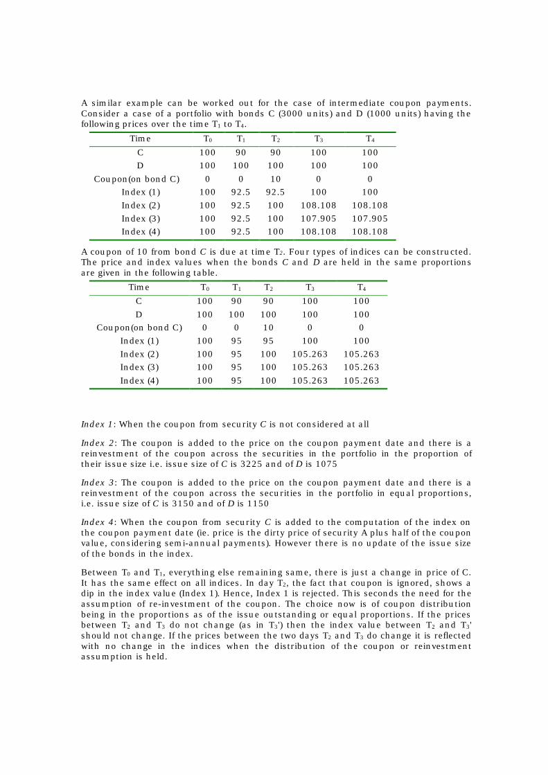
A similar example can be worked out for the case of intermediate coupon payments. Consider a case of a portfolio with bonds C (3000 units) and D (1000 units) having the following prices over the time T1 to T4.

Time T0 T1 T2 T3 T4 C 100 90 90 100 100 D 100 100 100 100 100

Coupon(on bond C) 0 0 10 0 0 Index (1) 100 92.5 92.5 100 100 Index (2) 100 92.5 100 108.108 108.108 Index (3) 100 92.5 100 107.905 107.905 Index (4) 100 92.5 100 108.108 108.108

A coupon of 10 from bond C is due at time T2. Four types of indices can be constructed. The price and index values when the bonds C and D are held in the same proportions are given in the following table.

Time T0 T1 T2 T3 T4 C 100 90 90 100 100 D 100 100 100 100 100

Coupon(on bond C) 0 0 10 0 0 Index (1) 100 95 95 100 100 Index (2) 100 95 100 105.263 105.263 Index (3) 100 95 100 105.263 105.263 Index (4) 100 95 100 105.263 105.263

Index 1: When the coupon from security C is not considered at all

Index 2: The coupon is added to the price on the coupon payment date and there is a reinvestment of the coupon across the securities in the portfolio in the proportion of their issue size i.e. issue size of C is 3225 and of D is 1075

Index 3: The coupon is added to the price on the coupon payment date and there is a reinvestment of the coupon across the securities in the portfolio in equal proportions, i.e. issue size of C is 3150 and of D is 1150

Index 4: When the coupon from security C is added to the computation of the index on the coupon payment date (ie. price is the dirty price of security A plus half of the coupon value, considering semi-annual payments). However there is no update of the issue size of the bonds in the index.

Between T0 and T1, everything else remaining same, there is just a change in price of C. It has the same effect on all indices. In day T2, the fact that coupon is ignored, shows a dip in the index value (Index 1). Hence, Index 1 is rejected. This seconds the need for the assumption of re-investment of the coupon. The choice now is of coupon distribution being in the proportions as of the issue outstanding or equal proportions. If the prices between T2 and T3 do not change (as in T3') then the index value between T2 and T3' should not change. If the prices between the two days T2 and T3 do change it is reflected with no change in the indices when the distribution of the coupon or reinvestment assumption is held.

Example 6: Consider two bonds A and B which are both redeemed in 10 years time at par. Bond A has a 10 percent annual coupon, whereas bond B is a zero-coupon one. During the next 10 years, bond A will pay out coupons to the value of 100 percent of the nominal capital, with the result that the average period to payout of all future cashflows is: (10/200) * ( 1+2+3+..+10) + (100/200)*10 = 7.75 years On the other hand, bond B has a average life of 10 years, since no payments are made prior to redemption.

Example 7 : The average duration of the discounted cashflows of a 10-year bond yielding 10 percent with a 10 percent coupon is 6.76 years, whereas that of a 10-year zero-coupon bond isstill 10 years. Thus, the latter has a duration which is 1.48 times as long as the former.

CHART 1: Government Securities Index

100.00

105.00

110.00

115.00

120.00

125.00

130.00

135.00

2001

0101

2001

0118

2001

0206

2001

0226

2001

0317

2001

0409

2001

0428

2001

0518

2001

0606

2001

0623

2001

0711

2001

0728

2001

0816

2001

0905

2001

0927

2001

1016

2001

1103

2001

1123

2001

1212

2002

0101

2002

0118

2002

0206

2002

0225

2002

0315

2002

0404

2002

0423

Date

Inde

x

CHART 2: Total Returns Index Jan-June 2001

100.00

102.00

104.00

106.00

108.00

110.00

112.00

114.00

116.00

118.00

2001

0101

2001

0106

2001

0112

2001

0118

2001

0124

2001

0131

2001

0206

2001

0212

2001

0217

2001

0226

2001

0303

2001

0312

2001

0317

2001

0323

2001

0330

2001

0409

2001

0417

2001

0423

2001

0428

2001

0505

2001

0512

2001

0518

2001

0524

2001

0530

2001

0606

Date

Inde

x

CHART 3: Total Returns Index Jun-Dec 2001

100.00

105.00

110.00

115.00

120.00

125.00

130.00

135.00

140.00

2001

0702

2001

0707

2001

0713

2001

0719

2001

0725

2001

0731

2001

0806

2001

0811

2001

0818

2001

0827

2001

0901

2001

0907

2001

0913

2001

0919

2001

0929

2001

1006

2001

1012

2001

1018

2001

1024

2001

1031

2001

1106

2001

1112

2001

1120

2001

1126

2001

1203

Date

Inde

x

CHART 4: Total Returns Index Jan-Jun 2002

100.00

105.00

110.00

115.00

120.00

125.00

130.00

135.00

140.00

145.00

150.00

2002

0101

2002

0107

2002

0112

2002

0118

2002

0124

2002

0131

2002

0206

2002

0212

2002

0218

2002

0225

2002

0302

2002

0308

2002

0315

2002

0321

2002

0328

2002

0404

2002

0410

2002

0417

2002

0423

2002

0430

2002

0507

2002

0513

2002

0518

Date

Inde

x