Groundwater flow modelling(450008)

Computer laboratories

dr. V.E.A. Post

Contents

Part I: Python 1

1 Calculating heads 51.1 Solution methods . . . . . . . . . . . . . . . . . . . . . . . . . . 5

1.1.1 Gauss-Seidel iteration using a spreadsheet . . . . . . . . . 51.1.2 Gauss-Seidel iteration using Python . . . . . . . . . . . . 61.1.3 Successive over relaxation . . . . . . . . . . . . . . . . . 81.1.4 Direct solution . . . . . . . . . . . . . . . . . . . . . . . 8

1.2 Regional flow example . . . . . . . . . . . . . . . . . . . . . . . 91.2.1 No-flow boundaries . . . . . . . . . . . . . . . . . . . . . 10

2 Calculating flows 132.1 Water budgets . . . . . . . . . . . . . . . . . . . . . . . . . . . . 132.2 Abstraction well . . . . . . . . . . . . . . . . . . . . . . . . . . . 14

3 Transient simulations 173.1 Abstraction well (transient) . . . . . . . . . . . . . . . . . . . . . 17

Part II: MODFLOW 19

4 Well field in a river valley 21

Part III: MicroFEM 27

5 Well in a semi-confined aquifer 29

6 Infiltration canal 33

Part IV: Linear algebra 37

7 Systems of linear equations 397.1 Linear equations . . . . . . . . . . . . . . . . . . . . . . . . . . . 397.2 Systems of linear equations . . . . . . . . . . . . . . . . . . . . . 40

3

8 Matrices 458.1 Definition . . . . . . . . . . . . . . . . . . . . . . . . . . . . . . 458.2 Special matrices . . . . . . . . . . . . . . . . . . . . . . . . . . . 458.3 Operations . . . . . . . . . . . . . . . . . . . . . . . . . . . . . . 468.4 Determinant . . . . . . . . . . . . . . . . . . . . . . . . . . . . . 488.5 Cramer’s rule . . . . . . . . . . . . . . . . . . . . . . . . . . . . 508.6 Inverse of a matrix . . . . . . . . . . . . . . . . . . . . . . . . . 51

References 53

Part I: Creating finite differencemodels in Python

Introduction

Nowadays, a wide selection of very powerful groundwater flow models isavailable.For almost every problem there is a code that suits your needs. But sometimes, thecode at hand is not just what you want. It may be that it doesn’t handle aspecificboundary condition or you want the output to be in a slightly different format tomake the post-processing easier. Wouldn’t it be convenient then if you have theskills to modify the original code a bit, or even to create your own model?

Moreover, if you have made (simple) models yourself, you also better under-stand how existing codes work. This may be helpful in a situation where the modelcrashes or behaves unexpectedly in a different way.

Fewer and fewer hydrologists possess the skills to modify or write computercodes. So, learning to write your own models will give you an advantage. In orderto do so, you also need to learn a programming language. A programming lan-guage is a set of functions and statements that allow you to pass commands on tothe computer. There are dozens of different programming languages available. Ex-amples include Visual Basic, Pascal, C, FORTRAN, Python and many, many more.In this course we will use Python. Python is a so-called command-line interpreter:you type in the commands that are subsequently executed. These commands canbe combined into a program which we call a script. The advantage of using Pythonis that lots of the things you would normally have to worry about as a program-mer have already been done for you. For example, creating plots and charts isextremely easy because the statements to send graphics to the screen have alreadybeen programmed. You can simply use the commands included in Python and itslibraries like matplotlib instead of figuring out all this complicated stuff yourself.

Another advantage of Python is that it is becoming widely used in various partsof the scientific community. Popular geographic information systems like ArcGISand GRASS also have Python functionality. In the groundwater industry, MAT-LAB, another interpreted programming language, is still the standard, althoughthat also slowly starts to change. The reason that we do not use MATLAB inthiscourse is that (i) Python is just as good and sometimes even better than MATLABand (ii) Python is open-source software. The latter means that there are no licens-ing issues and that you can install and work with Python on any computer, forexample at your home or on a laptop during your fieldwork.

So, in short, being able to write your own modeling code helps you to betterunderstand what you are doing if you are using an existing model. Also, it gives

3

Chapter 0

you the ability to modify and improve models or create custom-made models. Inthe learning process, you will become familiar with the basics of programminglanguages, which you can apply to other areas outside groundwater flowmodeling.

It is assumed that you are familiar with the basics of Python. If not, or if youwant to refresh your memory, then first familiarize yourself by going through thePython tutorial, which is available from your instructor.

4

Chapter 1

Calculating heads

1.1 Solution methods

During the lectures we have looked at the solution of unknown heads at theinteriornodes of a grid for which the heads at the boundary nodes are known (Dirichletboundary condition). We have seen that by ‘moving’ the so-called five-star op-erator through the grid, the head at each node could be calculated as a functionof the heads in the neighboring nodes. Calculating the heads once, however, wasnot enough to obtain the final solution. Instead, we started with an initial guessand then repeated the calculations until the heads no longer changed significantly(iteration).

1.1.1 Gauss-Seidel iteration using a spreadsheet

Such calculations are easily done by computers. Before creating a program inPython, let’s look at how we can use a spreadsheet to do these calculations. Sup-pose we have a grid as in figure 1.1 with the heads given for each cell on the modelboundary.

Figure 1.1: Simple mesh with heads fixed on the boundaries.

We can easily imagine the cells of a spreadsheet to coincide with the nodes ofthe model mesh. To do the calculations, proceed as follows:

• Open your spreadsheet program.

5

Chapter 1

• Type in the fixed head values at the cells representing the model boundary.

• Type a formula in the upper left interior cells that calculates the average ofthe heads in the 4 neighboring cells (see figure 1.2).

• Copy this formula to the remaining interior cells.

Figure 1.2: Entering the formula for Gauss-Seidel iteration in Excel.

It is that easy! The only thing is that, depending on the spreadsheet you use,you may need to iterate manually. In Microsoft Excel, this is done automatically ifyou select Tools→ Options and then on the Calculations tab enable the Iterationoption.

1.1.2 Gauss-Seidel iteration using Python

The advantage of using a spreadsheet is that it is easier to envisage the modelstructure because, like a finite-difference model, a spreadsheet consists of cells. Inthe remainder of the exercises, however, we will use Python because ofits muchgreater flexibility. As an example, take a look at the following Python-script, whichdoes exactly the same as what we did before in our spreadsheet.

from numpy import array

h = array([[4., 5., 6., 7.],[4., 0., 0., 7.],[4., 0., 0., 7.],[4., 5., 6., 7.]])

6

Python

dummy = h.shapenrow = dummy[0]ncol = dummy[1]

print ’Head matrix is a ’, nrow, ’ by ’, ncol, ’ matrix.’

ni = 1conv_crit = 1e-3converged = False

while (not converged):max_err = 0for r in range(1, nrow - 1):

for c in range(1, ncol - 1):h_old = h[r, c]h[r, c] = (h[r - 1, c] + h[r + 1, c] + h[r, c - 1] + h[r, c + 1]) / 4.diff = h[r, c] - h_oldif (diff > max_err):

max_err = diff

if (max_err < conv_crit):converged = True

ni = ni + 1

print ’Number of iterations = ’, ni - 1

print h

At first sight, this may look incomprehensibly complicated. It is certainly morecomplicated than entering the formulas in a spreadsheet. But if you get usedto pro-gramming it will become much easier to ‘read’ such scripts. Note how indentationis used to structure the script. In fact, you have to indent in Python, otherwise itwill complain! Try if you can understand what is going on here and then answerthe following questions:

• What is the purpose of the variable converged?

• What values does the shape variable return? Can you think of a reason whyit is better to use ‘shape’ to define the number of rows and columns ratherthan just assigning fixed values to these variables yourself?

• What is the name of the variable that is used to store the number of iterations?

• How does the program know that it only needs to calculate the interiornodes?

Exercise: The script is available on Blackboard. Download it to a local diskand open it in Python (simply by clicking File→ Open and selecting it). The scriptis opened in the script editor and can be run by pressing F5. Investigate the effectsof the convergence criterion and initial head guess on the number of iterations. Setthe convergence criterion to different values and note the number of iterations. Dothe same for the initial heads of the interior nodes.

7

Chapter 1

1.1.3 Successive over relaxation

A way to speed up the convergence is to use Gauss-Seidel iteration in combinationwith successive over relaxation (SOR). In this method, the difference between thecalculated value at the new iteration interval and that of the previous iterationin-terval c = hm+1

i,j − hmi,j is multiplied by a relaxation factorω. The new value of

hm+1

i,j becomes:

hm+1

i,j = hmi,j + ωc (1.1)

This equation can be written as:

hm+1

i,j = (1 − ω)hmi,j + ωhm+1

i−1,j + hm+1

i,j−1+ hmi+1,jh

mi,j+1

4(1.2)

Exercise: Open the example script of Gauss-Seidel iteration and modify it insuch a way that it can incorporate SOR. What extra variable(s) are needed? Notethat maxerr can become negative with SOR and that you need to take care that youcompare the absolute value of maxerr to the convergence criterion. Use a value ofω = 1.1.

The number of iterations is now . . . . . . . Increase the value ofω and run thescript again. Note that whenω > 1.25 the number of iterations increases comparedto the script without SOR! This is because for high values ofω the calculated headsduring the first iterations overshoot the final ‘true’ values and it takes some time toconverge back towards these values.

1.1.4 Direct solution

The previous exercise shows that the heads at the interior nodes are readily calcu-lated using Gauss-Seidel iteration, either with or without SOR. Iterative solutions,however, are not the most efficient way to solve the system of finite differenceequations. Direct solution methods are an alternative, more efficient way and areeasily applied in Python. Remember that a system of linear equations (such asthefinite-difference expressions for this problem) can be written in matrix form:

[A]~h = ~f (1.3)

where[A] is a coefficient matrix,~h a column vector of unknown heads and~f acolumn vector containing all known values.~h follows from:

~h = [A]−1 ~f (1.4)

where[A]−1 is the so-called inverse of[A].For the problem presented above, write down a finite-difference expression for

each unknown head at the interior nodes. The result is a system of 4 linear equa-tions with 4 unknowns. Transfer all known values (the heads at the boundaries)to the right-hand side and express the system of equations in matrix format. Then

8

Python

use Numpy’s linear algebra package to solve for~h (see page 19 – 20 of the Pythontutorial on how to do this). Did you get the same result as before?

Although direct solution methods are more efficient than iterative methodsthey require large amounts of computer memory for real-world numerical mod-els. Therefore, most codes use solution schemes that combine the best ofbothworlds of iterative and direct solution techniques.

1.2 Regional flow example

The previous example was very basic and not of much use in real-world model-ing. In the next example, we will use our numerical model to analyze flow systemsin a topographically-driven groundwater system. In the course ‘Groundwater hy-draulics’ you derived an analytical solution for this problem and did a numericalcalculation with FlexPDE. We will now modify our script so we are able to solvethe problem ourselves. We will combine the model with the powerful graphicalcapabilities of Python’s Matplotlib package to visualize the output. In that way,wehave already created a tool that starts to look like the industry-standard modelingpackages!

Take the script for Gauss-Seidel iteration with SOR as your starting point. Firstsave the script under a different name. Set the value of omega toω = 1.8 and setthe convergence criterion to1 · 10−5. As a first step, we will increase the numberof rows and columns of the model from 4 by 4 to 26 by 26. An easy way to sois to use the function zeros() to create the matrix h. In that way, all the startingheads will be set to 0 automatically. Look up how the function works and insertthe appropriate statement in the script. Note that you have to import the functionzeros() from numpy, just like the functionsin() andpi (see below).

We use the same configuration as for the exercise in ‘Groundwater hydraulics’,so our model will measure 500 by 500 m. What will be the width of the grid cells(note: we have a mesh-centered grid!). Declare a variable called dx andset itsvalue to the appropriate grid cell width. We will use square cells, so there is noneed to define the height of the cells explicitly.

The heads at the top of the model can be defined by superposition of 2 sinefunctions with different wavelengths. This is expressed in the formula:

h = A1 ∗ sin(k1 ∗ x) +A2 ∗ sin(k2 ∗ x) (1.5)

whereA1 andA2 are the amplitudes of the respective waves,k = 2 ∗ πn/L, n isthe wave number andL is the width of the model. Modify the script to include theparametersL, A1, A2, n1, n2, k1 andk2. Set the values ofA1 = A2 = 5.0 m andn1 = 1 andn2 = 2.

Equation 1.5 contains the variablex, so we need to knowx for each columnin the grid. Try to find the right statements to accomplish this and then implementequation 1.5 in the script. Once you have done this, you’re almost ready to start thecalculations. As a final step, include this statement at the beginning of the script:

9

Chapter 1

from numpy import *

Include the following statements at the end of the script to produce graphicaloutput:

close()f = figure()[X, Z] = meshgrid(linspace(0, L, ncol), linspace(0, -L, nrow))contourf(X, Z, h)

colorbar()

[dhz, dhx] = gradient(h)quiver(X, Z, -dhx, dhz, color = ’w’)

Look up what these functions do. Can you understand what they mean? If youdo you’re now ready to start calculating your first real-world, self-made groundwa-ter flow model!

1.2.1 No-flow boundaries

Note that we didn’t worry about the no-flow boundary at the bottom of themodelin the previous exercise. How can you see from the contour lines of the hydraulicheads that the bottom boundary is not a no-flow model? In the next exercise wewill implement the no-flow boundary. We only need to make a few adjustments.

Remember from the lectures that a way to incorporate no-flow boundaries isto add imaginary nodes outside the model domain. The type of grid determineshow the no-flow boundary is implemented. For a mesh-centered grid, the gradientacross the boundary becomes zero (the condition for no-flow) ifhi,j+1 = hi,j−1,wherehi,j+1 the head at the the imaginary node outside the model domain andhi,j−1 is the head at first node inside the model boundary.

We will expand our matrix at the bottom with one additional row, representingthe imaginary nodes. To do so, change the declaration of matrix h. Then implementthe no-flow boundary by adding the following line:

h[-1, :] = h[-3, :]

Specifying-1 at the row index is short in Python for the last row;-3 indicatesthe third-last row. The colon at the column index means ‘all columns’. So thisstatement assigns the heads of the third-last row to the heads of the last row, for allcolumns. Where would you insert this line into our script? If you add it your scriptis almost ready to handle the no-flow boundary. Before you start the calculationthough, you need to make some minor changes to the statements that produce thegraphics. These prevent the imaginary cells from being displayed. The correctsyntax is:

10

Python

close()f = figure()[X, Z] = meshgrid(linspace(0, L, ncol), linspace(0, -L, nrow - 1))contourf(X, Z, h[:-1, :])

colorbar()

[dhz, dhx] = gradient(h[:-1, :])quiver(X, Z, -dhx, dhz, color = ’w’)

Only 3 lines are different. Study the differences and make sure you knowwhatthey mean. Then start the calculations and pay particular attention to the headcontours near the bottom boundary. What has changed?

11

Chapter 2

Calculating flows

2.1 Water budgets

In the previous examples the convergence criterion controls the accuracy of thesolution. As a second check on the accuracy, a water balance can be set up. Re-member from the lectures that for a 2D model with square grid cells:

Q = −k∆h

∆x∆x = −k∆h (2.1)

Assume that the hydraulic conductivity (k) is 10 m/d. Extend the script of theregional flow example to calculate the water balance of the whole model domain.Calculate inflow and outflow of each model boundary except for the bottombound-ary. Make sure to adopt a sign-convention for inflow (+) and outflow (-). Fill in thetable below.

Table 2.1: Water budget for regional flow example

flow component magnitude

qleft . . .qright . . .qtop . . .qbottom . . .

qtotal . . .

Compare the net inflow (inflow - outflow) to the magnitude of the inflow/outflow.Is the error in the water balance acceptable?

Note that thenet flow over the top model boundary is basically zero but thatthe inflow and outflow components themselves over this boundary are not. Whatare the magnitudes of the inflow and outflow over the top boundary?

13

Chapter 2

2.2 Abstraction well

In this exercise we calculate the drawdown due to a well that fully penetratesaconfined aquifer. Flow is horizontal and the aquifer is isotropic. Under these con-ditions and when∆x = ∆y, the formula for Gauss-Seidel iteration takes the fol-lowing form (check your lecture notes):

hi,j =hi−1,j + hi,j−1 + hi+1,j + hi,j+1 + ∆x2R/T

4(2.2)

whereT is the transmissivity (m2/day) andR is the volume of recharge/dischargeper unit time per unit surface area. R and Q are related by (for square grid cells, so∆x = ∆y):

R =−Q

∆x2(2.3)

Transmissivity isT = 300 m2/day. The well is located atx = 0, y = 0 and hasa discharge ofQ = 2000 m3/day. The value ofR is for the infinitesimal volumearound the well (figure 2.1). Outside this volumeR = 0.

Figure 2.1: Finite difference grid for abstraction well exercise. ModifiedfromWang and Anderson (1982).

Because the equipotential lines will be cylindrical around the well, the problemis symmetric and we only need to consider one quarter of the problem domain.Let’s model the lower-right quardrant so the left and upper boundaryare the no-flow boundaries (figure 2.1). The analytical solution for this problem is given bythe Thiem equation:

h = h0 +Q

2πTln

r

rmax(2.4)

whereh0 is the head before pumping andrmax is the radius of influence of thepumping well. Assume for this exercise thatrmax = 2000 m. Note that al-though time is not in this formula, this is actually not a steady-state problem: The

14

Python

Thiem equation calculates the heads for a givenrmax. Check your lecture notes of‘Groundwater hydraulics’ to see howrmax varies with time.

As before, take the script for Gauss-Seidel iteration with SOR as your startingpoint. Set the value of omega toω = 1.8 and set the convergence criterion to1 · 10−3. Use a (mesh-centered) grid of 12 rows by 12 columns (of which thefirst row and column are imaginary nodes!). Use∆x = ∆y = 200 m. Make thefollowing modifications to the script (not all of them are straightforward, soask forhelp if you don’t succeed yourself):

• Calculate the distance of each node to the well and find the nodes whosedistance most closely match the radius of influence (rmax = 2000 m). Setthe heads of these nodes and of those outside the radius toh = 10 m. Set thestarting heads of all remaining nodes toh = 5 m.

• Include lines to make the left and upper boundaries no-flow boundaries.

• Modify the statements that perform the Gauss-Seidel iteration in such a waythat they can take into account the abstraction well (equation 2.2).

• Make sure that the heads are only calculated for the nodes that are partof thearea of influence of the well. In other words, don’t calculate the heads of thenodes that you have set toh = 10 m. You will have to think of a smart trickto accomplish this.

• Include the options for graphical output at the end.

• Finally, add a program line to calculate the analytical solution with the Thiemequation so you can compare it to the numerical result.

You will find that the analytical and numerical results agree very well. Youcould include a water balance calculation but that involves quite a bit of adminis-tration since the inflow here is not simply through the right and bottom grid bound-aries but across the circumference formed by the sides of the cells that are markthe radius of influence.

15

Chapter 3

Transient simulations

3.1 Abstraction well (transient)

The previous exercises all assumed steady-state conditions. In this exercise thewell-drawdown problem will be expanded to a transient simulation. As before,only the lower-left quadrant, measuring 2000 by 2000 m, is considered but now allthe boundaries are no-flow boundaries and the cell size is∆x = ∆y = 100 m.

The numerical results will be compared to the analytical solution by Theis thatcalculates the drawdown at a radius (r) from the well:

h0 − h =Q

4πTW (u) (3.1)

where

W (u) =

∫

∞

u

e−ψ

ψdψ (3.2)

and

u =r2S

4Tt(3.3)

W (u) is called the well functions and is usually tabulated in textbooks. It is alsoimplemented in Python so there is no need to look it up: you simply calculateit with Python! The input file for this exercise has been prepared for you(it isavailable via Blackboard). Study it and answer the following questions:

1. What is the function of the parameters alpha and nsteps?

2. What is the size of the time steps?

3. See if you can find the lines that calculate the analytical solution. What isthe Python equivalent of the well functionW (u)?

4. At what distance are the analytical solution and the numerical solution com-pared?

17

Chapter 3

After you have studied the script, run it and observe the graph that is produced.It compares the fit between the analytical and numerical results.

1. At what time do they start to deviate and why is this?

2. What causes the smaller deviations before this time?

3. Modify the script to have it perform fully-implicit calculations. What is theeffect on the number of iterations?

4. Then change to a fully-explicit formulation. What happens? To prevent this,only one line of the code needs to be changed. Which one? And how wouldyou change it? Make the change and discuss the implications.

To finish, uncomment the lines that produce the 3D graph of the heads duringthe calculations. A ‘movie’ will be displayed on the screen that shows the changein heads over time.

In a relatively short time you have mastered Python, learned to program yourown modelling codes and became a movie producer. Not bad, don’t you think?!

18

Part II: Creating finite differencemodels in MODFLOW

Chapter 4

Well field in a river valley

This exercise is a modified version of tuturial 3 from Chiang (2005). It serves to (1)become familiar with the input file structure of MODFLOW, (2) compare 3D andquasi-3D vertical discretization methods, (3) illustrate the use of the MODFLOWWell and River packages and (4) practice the interpretation of the water balance.The files that are needed for this exercise are available on Blackboard.

Problem description

A river flows through a valley, which is bounded to the north and south by im-permeable granite intrusions (figure 4.1). The hydraulic heads in the valleyat theupstream and downstream model boundaries are known. The river forms part of aphreatic aquifer, which overlies a confined aquifer of a variable thickness. A siltylayer with a thickness of 0.5m separates the two aquifers. A well field consisting of3 pumping wells is to be installed, which will be abstracting groundwater at a pro-posed rate ofQ = 500 m3/day from the confined aquifer. The question is how thatwell field will affect the discharge of the river, which provides water to avaluableecosystem downstream.

The relevant hydraulic parameters of the aquifer system are listed in table 4.1.

Model setup

Several files are available on Blackboard with information on the geometry and theheads of the aquifer system. Start by downloading these files and put themin yourworking directory.

We will initially simulate the system with a quasi-3D model (steady-state).That means that the silt layer is not explicitly included in the model. Instead, weenter an appropriate value of the vertical leakance. Hence, the head in the silt layeris not calculated but the exchange of water between the upper and the lower aquiferthrough the silt layer is. To set up the model, proceed as follows:

Chapter 4

Figure 4.1: Configuration of the model

• Create a new model in PMWIN and lay out the grid. Use 2 model layers(each representing a single aquifer), 20 rows and 27 columns. You canfindthe model extent from figure 4.1.

• Load the basemap for this exercise by going to Options→ Map in the grideditor. Right click on the DXF File field and open the file basemap.dxf(which you just copied from Blackboard). Make sure you check the box infront of the filename.

• The map will be loaded but it is shifted relative to the grid. You can movethe grid by selecting Options→ Environment and entering Xo = 200 and Yo= 6000 in the Coordinate System tab.

• You can already refine the grid at the location of the well field. To do so,leave the Grid Editor and enter it again. Then halve the widths of the columns8 through 14 and rows 7 through 12 by repeatedly right-clicking each of themand specifying the appropriate refinement factor (= 2). Your grid will looklike the one in figure 4.2.

• Set the appropriate layer properties (confined or unconfined) underGrid →Layer property. Select ‘User defined’ for the Transmissivity and Leakance.

• Set the boundary conditions. The granite hills will be represented by inactivegrid cells. Use the Polygon feature of the PMWIN editor to accurately delin-eate the hills. You can copy the inactive cells to the second model layer byactivating the ‘Layer copy’ button on the toolbar. The boundary condtition

22

MODFLOW

Table 4.1: Aquifer system parameters for river valley exercise

Parameter magnitude units

Aquifer 1 (phreatic)Horizontal hydraulic conductivity (kh) 5 m/dayVertical hydraulic conductivity (kv) 0.5 m/dayPorosity (n) 0.2

Silt layer (confining unit)Horizontal hydraulic conductivity (kh) 0.5 m/dayVertical hydraulic conductivity (kv) 0.05 m/dayPorosity (n) 0.25

Aquifer 2 (confined)Horizontal hydraulic conductivity (kh) 2 m/dayVertical hydraulic conductivity (kv) 1 m/dayPorosity (n) 0.25

RiverStage (upstream/downstream) 19.4/17 mBottom elevation (upstream/downstream) 17.4/15 mWidth 100 mRiver bed hydr. conductivity 2 m/dayRiver bed thickness 1 m

at the upstream and downstream valley boundaries will be fixed heads. Thevalues of the fixed heads (which you need to enter later under Grid→ Initialand prescribed heads) are in the file fixedheads.dat.

• Specify the layer top elevations by going to Grid→ Top of Layers and load-ing the files top1.dat and top3.dat. Specify the layer bottom elevations bygoing to Grid→ Bottom of layers. Donot accept the option for determiningthe bottom elevations from the top elevations of the underlying layers. Setthe bottom elevation of layer 1 to the elevation of the top of the silt layer,which is stored in the file top2.dat. Set the bottom of layer 2 to a constantvalue of 0 m.

• Select Parameters→ Time and set the time units to days and specify that thiswill be a steady-state simulation.

• Specify the transmissivity, vertical leakance, horizontal hydraulic conductiv-ity and effective porosity. You can calculate these number with the data fromtable 4.1 and the thicknesses of the layers (look these up in the model). Takecare of the following:

1. Note that the thickness of the confined aquifer is not constant. There-fore, the transmissivity of this layer varies. You can calculate it au-

23

Chapter 4

tomatically by using a trick. First, set the hydraulic conductivity to 2m/day in each cell (use the Reset matrix function). Then load the filetop3.dat which contains the aquifer top elevation. Since the bottom el-evation is 0 everywhere, the numbers in this file equal the thickness ofthe aquifer. Before pressing the Ok button to load the file, select theoption multiply. The numbers currently in the grid will be multipliedwith the numbers in the file.

2. The vertical leakance is only defined for the first model layer. It is notdefined for the bottom model layer (you can check this in the MOD-FLOW input file later). It is dependent on the thicknesses of all 3 hy-drostratigraphic units. It is a bit harder to calculate than the transmis-sivity so the file has been prepared for you. It is called vcont1.dat.Check if you understand how these values have been calculated. Dothis by calculating the value for a particular cell by hand.

• Add the river. MODFLOW requires that the river data (i.e. stage, bottomelevation, and riverbed conductance) are specified for each grid cell that theriver intersects. Go to Models→ MODFLOW → Flow packages→ River.Use the Polyline input method to accurately trace the river. Vertices areadded by left-clicking; defining the polyline is cancelled by right-cliking. Tocomplete the polyline, left-click the last vertex you specified again. Thenright-click the leftmost (upstream) vertex and enter the data for this rivernode (the values are in table 4.1). Do the same for the rightmost (down-stream) vertex. You do not need to enter the values for the other vertices:PMWIN interpolates between the two outer vertices, which makes life a biteasier.

After entering all the data make sure that you did not forget anything. Check-ing the input is an important step in groundwater modelling, especially if you arerunning models that take a couple of hours to finish. Then run MODFLOW.

Graphical user interfaces like PMWIN are great in that they tremendouslyfa-cilitate data entry. The drawback is that a lot of the ‘action’ takes place behind thescenes and remains hidden from the user. For example, PMWIN generates all theinput files that MODFLOW needs. Usually, there is no need to edit these input filesyourself but as an academic you are naturally curious of how they look. Moreover,sometimes a graphical user interface does not support all the options of acode andyou may need to modify the input files directly. Therefore, before proceeding, goto your working directory that contains all the files of this model. Look up the filethat has the extension ‘.nam’. It contains a list of the filenames that are usedbyMODFLOW. Look up these files and try to find out what their purpose is andwhatdata they contain.

Then plot the hydraulic head distribution using Tools→ 2D Visualization. Alsocheck the water balance. You can use either the water budget option of PMWIN oropen the file ‘output.dat’ in a text editor. How much water enters the model domain

24

MODFLOW

Figure 4.2: Model grid

through the upstream valley boundary? And how much water leaves through thedownstream boundary? The river is both a source and a sink of water tothe aquifer.But on the whole, is this a losing or a gaining river? Note that the water balanceerror is basically zero. Write down the numbers as we will compare them to themodel with groundwater abstraction later.

Then run the model again but with the 3 wells in place in the confined aquifer.Each withdraws water at a rate of 500 m3/day from layer 3, which is entered underModels→ MODFLOW→ Flow packages→ Well.

Again, observe the head distribution. This time, also use PMPATH to draw flowlines. Then check the water budget again. What percentage of the pumpedwaterderives from groundwater and how much is infiltrated river water? By how muchhas the river discharge decreased at the downstream model boundary compared tothe natural situation?

Then change the model from a quasi-3D to a full 3D model. The easiest wayto do this is to:

• go to Grid→ Mesh size and subdivide the second model layer into 2 layers.Do this by pressing PgDn to go to the second model layer. Then you canright-click on any cell and type 2 in the Layer refinement field.

• set the appropriate layer properties under Grid→ Layer property. Select‘Calculated’ for the Transmissivity and Leakance. This means that the valuesof these parameters will be calculated by MODFLOW using the hydraulicconductivities and layer top and bottom elevations.

25

Chapter 4

• set the boundary conditions. The values for the two aquifers remain thesame as before. The inactive cells of the second model layer (the silt layer)are the same as for the aquifers, but the boundaries on the upstream anddownstream valley boundaries are no-flow boundaries (we assume thatflowis purely vertical in the silt layer so there is no flow over the boundary).

• set the layer top and bottom elevations using the values from the files youused earlier.

• set the horizontal and vertical hydraulic conductivity and effective porosityto the values from table 4.1.

If you run the model you will get basically the same results as with the quasi-3D model. Check this by comparing the head distribution and the water balance.

As a final exercise, do a sensitivity analysis for the hydraulic conductivity ofthe river bed. As you can imagine, this parameter is extremely difficult to quantifyand it will also probably be quite variable along the streambed. We have usedavalue of 1 m/day but why could they not range between 0.5 to 2 m/day? Re-runthe model using these extremes and investigate the effect on the hydraulic headdistribution and the water budget. Don’t let these result make you lose faith inmodels but consider them a lesson in critical thinking.

26

Part III: Creating finite elementmodels in MicroFEM

Chapter 5

Well in a semi-confined aquifer

This exercise serves to illustrate the basic capabilities of MicroFEM. A well ab-stracts groundwater at a constant rate of 50 m3/hour from a confined aquifer. Un-der natural conditions uniform flow occurs in a WSW direction, parallel to the longsides of a rectangular model. We will model the head distribution in the aquifer andcalculate a water balance.

1. Create a network using the FemGrid generator: Choose Files→ New gridand in the window that appears select ‘Create new grid’ and press OK. In thesubsequent window, enter a descriptive model name. This is required beforeyou can continue. By pressing OK you enter the grid editor.

In the upper righthand corner you see 3 tabsheets in which you enter therequired information to create the grid. You will have 5 fixed nodes: fourat the corners of the grid and 1 for the well. Only 3 fixed nodes are default,however. To change this, type 5 in the edit field and click the button ‘Changenumber to’. Now there will be 5 rows for which you can enter the x- andy-coordinates. The coordinates are (1000, 0), (13000, 3000), (12000, 7000)and (0, 4000) for the model boundary corner nodes and (4500, 3000) for thewell. Define the segments and regions as explained during the lecture. Setthe distance between nodes to 400 m on the model edges and to 250 m in themodel interior.

Then press the button ‘Fixed nodes’ in the toolbar at the bottom of yourscreen. The fixed nodes are created and displayed on your screen.Thecaption of the button has changed to ‘Nodes on segments’. Press it againand observe what happens. Press it again and again and each time make sureyou understand what is going on. Your network will have 866 nodes (figure5.1). Then you can either save the network (recommended) or choose thenumber of aquifers (which is 1) and start entering the hydraulic parameters.

2. Find the dimensions of the rectangular model domain, i.e. the exact modelwidth and length. Do this by placing the cursor in one of the 4 corner nodesand assigning the variabler to all nodes for a parameter (e.g. h0) in the input

Chapter 5

Figure 5.1: Rectangular model area with short east- and western and longnorthernand southern boundaries.

mode. Look up the meaning of this parameter in the help file! What are themodel dimensions?

3. We start with a confined aquifer so the vertical resistance of the first modellayer should be set to 0 (which is interpreted as infinite by MicroFEM). Thetransmissivity isT = kD = 800 m2/day. These parameters are entered inthe input mode.

4. Groundwater flow is in a WSW direction parallel to the long sides of themodel. The head at the eastern boundary is 20 m and the hydraulic gradientis 0.001. Assign head values to all model nodes by marking the east modelboundary in the walking mode and using a formula that calculates the head asa function of the head on the eastern boundary, the gradient and the variabled (which represents the distance to the nearest marked node).

5. Make a contour map in the drawing mode to check that the heads were en-tered correctly. Double-check by going to the western boundary: the headshould be 7.631 m here.

6. Go to the fixed node that contains the well (coordinates 4500, 3000). Notethat it has the label ’fixed node 5‘ so it is easily found by using the ‘Jump tonode’ function in the walking mode. Press F12 or the ‘Jump to node’ button,select ‘Next label’ and choose ‘fixed node 5’ from the pull-down list. Makesure that you ended up in the right node (check the coordinates as well asthe label in the lower-right corner of the screen) and then assign the welldischarge to this node in the input mode. Well discharge has a positive valuein MicroFEM, contrary to MODFLOW! Also change the name (= the valueof the parameter label1) of this node from ‘fixed node 5’ to ‘Well’.

30

MicroFEM

7. Run the model by going to Calculate→ ‘Go calculate’. Why is there noconvergence?

8. Restore the natural hydraulic head situation by repeating step 4. Then fixthe heads on the eastern and western model boundaries. Mark the nodesonthese boundaries and make sure that the head of the first aquifer is selectedin the parameter list. Then use the ‘Toggle heads for marked nodes’ functionto fix the heads: The word ‘fixed’ will appear in the parameter list for themarked nodes.

9. Run the model again by going to Calculate→ ‘Go calculate’. This time, asolution is found. Why?

10. Draw the hydraulic head contours in the drawing mode. You can overlay aset of flow vectors to visualize the flow. Explore the options of the drawingmode by clicking around a bit.

11. Go to the node that contains the well to draw the flowlines to delineate thecapture zone of the well. Specify a number of 12 flowlines, a timestep of100 years, layer thickness of 40 m and a porosity of 30 %. What is the widthof the capture zone? Why are the isochrons curved?

12. Set up a water balance for the entire model. You can find the water balanceoptions in the walking mode. What is the inflow through the eastern modelboundary? And what is the outflow over the western boundary?

13. We will now change the model from a confined aquifer with a well to asemi-confined aquifer without a well. Moreover, we set the transmissivitydownstream of the well to 300 m2/day. Thegroundwater table (h0) is setto the originalhydraulic heads under natural conditions. Make sure to makethe following changes:

• Assign a hydraulic resistance (= parameter c1) of 2500 days to theconfining unit.

• Set the groundwater table by marking the eastern boundary and enter-ing the formula (as in step 4 but now for h0 instead of h1): 20-0.001*d.

• Change the transmissivity downstream of the well from 800 m2/day to300 m2/day. Do this by marking the appropriate nodes and assigningthe value of 300 m2/day to the marked nodes only in the input mode.

• Remove the well from the model (i.e. set the discharge to 0).

14. Calculate the heads. Also make a contour plot of h1-h0 through the followingsteps:

• Go to Project→ Project Manager to add an extra variable for each nodethat can be used to hold intermediate results. A window will appearwith a list of all MicroFEM files for this model.

31

Chapter 5

• Click the button with the bright-green + sign, select Xtra worksheet,check ‘New’ in the ‘Create data from’ field (otherwise you will beasked for a file to read the data from) and click OK. You can choose tohave as many registers (= new input fields) as you like, but 1 will beenough for our purposes.

• Note that the project manager is also the place to add special types ofboundaries. Close the project manager and note that an new tab hasbeen created that is called Xtra. It contains an edit field for a variablex1. This variable can contain any value we assign to it without affectingthe calculations. Since we are interested in the head difference acrossthe semi-confining unit we assign the result of the formula ‘h1-h0’ toall nodes.

The positive values of the head difference indicate that there is upward seep-age in the whole model domain. Check the water balance. How much is theupward seepage through the semi-confining unit?

15. Then activate the well again. Calculate the model and check the water bal-ance. Indicate the zones of upward seepage and infiltration by drawing thedifference between h0 and h1. Calculate the volumetric rate of upward seep-age/infiltration (in m3/day) for each node (in the Xtra worksheet). Checkyour calculation by comparing it to the water balance.

16. What proportion of the well discharge infiltrates through the semi-confiningunit and what proportion derives from regional groundwater flow?

32

Chapter 6

Infiltration canal

This problem serves to demonstrate the supremacy of finite element models overfinite difference models when it comes to grid design. A shallow infiltration canalloses water to two fully penetrating drains. The drains are 120 m apart, with waterlevels at 40 and 35 m (left and right side, respectively) above an impervious base.The water level of the 5 m deep and 25 m wide infiltration canal is 55 m (seefigure 6.1). The aquifer is homogeneous and isotropic, with hydraulic conductivityk = 25 m/day.

We will simulate this problem as a profile model. A hollow groundwater tablewill develop between the infiltration canal and the drains. The grid must be de-formed in order to represent the saturated part of the model domain. Rememberthat at the groundwater table the pressure of the waterP = Pabs − Patm = 0 sothat the hydraulic headh = z+ P

ρg= z, wherez is the so-called elevation head. In

other words, the elevation of a water table node above a reference level(in this casethe impermeable base) needs to be equal to the calculated head. The mesh needsto be adjusted after each calculation so that the top model boundary coincides withthe groundwater table.

1. In order to save you some time, the configuration of the network has alreadybeen prepared and can be found on Blackboard. The fixed nodes, trian-gles and quadrangles that make up the mesh are stored in the file ‘profilemodel.fen’. Open this file in MicroFEM by going to Files→ New Grid andpressing OK. A file selector window appears. Open the fen file and checkhow the FemMesh network has been defined.

2. Create the network and go to MicroFEM. Select 1 as the number of layers.A profile model is implemented in MicroFEM by assigning an infinite re-sistance to the upper confining unit (i.e., c1 = 0) and entering the hydraulicconductivity (k-value) instead of the transmissivity.

3. Then set up the model: assign fixed heads to the nodes that representthecanal and the drains and set the appropriate values for h1. Enter the trans-missivity (= hydraulic conductivty). As a preparation for subsequent steps

Chapter 6

Figure 6.1: Configuration of the flow problem of the infiltration canal

give the nodes that sit between the canal and the drains the label ‘water ta-ble’.

4. You are now ready to calculate the model for the first time. New heads willbe calculated, which provide a first estimate of the shape of the groundwatertable. We can use these to relocate the nodes at the top of the model domain.Take the following steps and follow these carefully (otherwise MicroFEMcould crash):

• Go to Export→ Special ASCII files and select CSV-file. For each nodeall the model parameters, together with the x- and y-coordinates, willbe exported.

• The trick is now to change the y-coordinates of the ‘water table’ nodesand set these equal to the head we just calculated (parameter h1). Youcould in theory do this in Excel but it’s a pain. Python is much bet-ter suited for this purpose. Remember also that this is only a smallfile but the output from a real-world model may not even fit in Excelsdatasheet. A file called ’readcsv file.py’ is available on Blackboard.Download it to the same directory where you saved the csv file. Thecomments in the file explain in detail what it does. Inspect the file andmake sure that you understand what is going on. Then run it.

• Return to MicroFEM and select Import→ Special ASCII files. SelectCSV-file and open the file you just saved in Excel. The new coordi-nates will be read and the nodes on the upper model boundary haveshifted downwards. The grid has been deformed and now is a betterapproximation of the shape of the saturated part of the model domain.

• With the nodes shifted, the shape of the elements is not necessarilyideal. Therefore we will let MicroFEM optimize the shape of the net-

34

MicroFEM

work. In the Walking mode, mark all nodes. Then go to the Alter gridmode and press F10 (‘Relocate marked nodes’). You can see the net-work being optimized. It doensn’t hurt to do this 2 more times to getthe most optimal grid.

• Now calculate the heads again and repeat the steps above until theshape of the grid (or the position of the groundwater table) no longerchanges. The flow problem is then solved.

In this example, the shape of the grid depends on the calculated heads. Theflexibility of finite element methods and the powerful capabilities of Micro-FEM allow you to solve this problem. Solving the same type of problem inMODFLOW is not so easy!

5. Draw flowlines starting atall nodes of the infiltration canal bed. Hint: givethese nodes the same label (e.g. ‘canal’).

6. Set up a water balance. How much water is lost to each drain?

7. If you have time left, you can play around with the hydraulic conductivityand see what effect it has. For example, change use a value ofk = 1 m/dayand note the effect on the head contours and the water balances. Or youcould introduce anisotropy (e.g.kh = 25 andkv = 1 m/day).

35

Part IV: Linear algebra

Chapter 7

Systems of linear equations

Numerical approximations of the governing equations for groundwater flow lead toa set of algebraic equations that can be solved for the unknown heads by (i) iterationor (ii) direct solution techniques. With direct solutions, the system of equations istransformed into matrices and the unknown heads are solved using the techniquesof linear algebra. Therefore, some knowledge these subjects is indispensable if youare working with numerical groundwater models.

This document is intended for self-study and will give you a basic comprehen-sion of the relevant topics for the practicing hydrologist. Some of the exercisesrequire the use of Python. Python provides support for matrix operations throughthe Numpy library. These are not described here but you are expectedto try andlook these up yourself in the on-line documentation for Numpy. A good startingpoint is the following website:http://docs.scipy.org/doc/numpy/reference/index.htmlBut of course, when in doubt or when you get stuck, do not hesitate to ask yourinstructor!

7.1 Linear equations

A linear equation is an algebraic expression with one or more variable in whicheach term is a constant or the product of a constant and a variable. Forexample:

h(x) = Ax+B (7.1)

whereh is the dependent variable,x is the independent variable,A is theslope orgradient andB is theintercept, i.e. the value ofh whenx = 0.

39

Chapter 7

x

h0 h1

qx

x1x0

Figure 7.1: Schematic cross-section depicting a confined aquifer with one-dimensional horizontal flow.

7.2 Systems of linear equations

Two variables

Recall that Equation 7.1 is the general solution of a one-dimensional partialdiffer-ential equation

∂2h

∂x2= 0 (7.2)

that describes the hydraulic headh in a confined aquifer between two canals as de-picted in Figure 7.1. As a demonstration example of asystem of linear equations,let’s try to determine the integration constantsA andB from boundary conditions.So instead of treatingh andx as the dependent and independent variables, respec-tively, their values become fixed by the following boundary conditions:

h∣

∣

x=x0

= h0 (7.3)

h∣

∣

x=x1

= h1 (7.4)

Combining conditions 7.3 and 7.4 with Equation 7.1 and yields a system oftwo linear equations:

h0 = Ax0 +B (7.5)

h1 = Ax1 +B (7.6)

in whichA andB are the unknowns andx0, x1, h0 andh1 are known constants. Ifwe wish to find the numerical values ofA andB we must findthe solution to this

40

Linear equations

system of linear equations. This means finding the values ofA andB so that bothEquation 7.5 and 7.6 are satisfied.

Assume thath0 = 10, h1 = 9, x0 = 50 andx1 = 1501. Let B now be thedependent andA be the independent variable so that we have:

B = 10 − 50A (7.7)

B = 9 − 150A (7.8)

One way to find the solution is to plot Equations 7.7 and 7.8 in a graph and tolook up the point where they intersect. This is shown in Figure 7.2. Obviously, thismethod can be inaccurate when the graph is drawn by hand and is not suitable forsystems of equations with more than 2 variables.

Exercise: Find the graphical solution to Equations 7.5 and 7.6 forA andB as-sumingx0 = 0 and the other parameters as listed above.

A better way would be to use the method of substitution. This involves reduc-ing the number of unknowns by expressingA as a function ofB using either oneof the Equations 7.7 or 7.8 and substituting the result into the other. The equationobtained this way can be solved forB. The value ofA is subsequently found bysubstituting the calculated value ofB in either Equations 7.7 or 7.8 and solving forA.

Exercise: Find the solution of Equations 7.7 and 7.8 by the method of substitu-tion. Verify that your answer is the same as in Figure 7.2. Note that the solutionis written as{(A,B)}, i.e. a set containing an ordered pair.

For the system described by Equations 7.7 or 7.8 there is one solution andtherefore it is called aconsistent system. Aninconsistent system on the other handhas no solution. For example, the linear system:

50A+B = 10 (7.9)

50A+B = 9 (7.10)

represents two parallel lines and therefore has no solution. This is denoted by anull or an empty set:∅ or {}. Note that substitution would yield10 = 9, which isa contradiction from which it is clear that there can be no solution.

A system of two linear equations with two variables will have an infinite num-ber of solutions when the two lines coincide. This occurs if the equations areamultiple of each other. For example:

50A+B = 10 (7.11)

100A+ 2B = 20 (7.12)1All having length units, for example m

41

Chapter 7

-0.050 -0.025 0.000 0.025 0.050A

5

10

15

20

B

B = 10−50A

B = 9−150A

(−0.01,10.5)

Figure 7.2: Graphical representation of Equations 7.7 and 7.8.

represent the same line in a plot ofA versusB. This is called adependent systemand the solution is either of these two equations:{(A,B) | 50A+B = 10}.

Three (or more) variables

To develop a system of linear equations of three variables, suppose we would liketo solve Equation 7.2 numerically. For this purpose, the domain betweenx0 andx1 is first discretized inton cells. The numerical approximation yields (central inspace, cf. lecture notes):

∂2h

∂x2≈hc−1 − 2hc + hc+1

(∆x)2= 0 (7.13)

or:2hc = hc−1 + hc+1 (7.14)

where the subscriptc indicates the cell number (1 ≤ c ≤ n). Suppose thatn = 5and that the heads in the first and fifth cells are fixed heads withh1 = 10 andh5 = 6. The heads in the nodesh2, h3 andh4 are then given by:

2h2 = 10 + h3

2h3 = h2 + h4

2h4 = h3 + 6

42

Linear equations

that can be written as a system of linear equations with three variables:

2h2 − h3 = 10−h2 + 2h3 − h4 = 0

− h3 + 2h4 = 6(7.15)

This system system of equations can be solved forh2, h3 andh4 by an algo-rithm calledGaussian elimination. It useselementary row operations to transformthe linear equations into a form that is easily solved. Application of these opera-tions does not change the solution of the system of linear equations. The operationsare:

1. Equations can be interchanged

2. An equation can be multiplied with a non-zero constant

3. An equation can be multiplied by a constant and added to another equation

As an example, first reverse the first and second equation in the system defined byEquation 7.15 (Operation 1):

−h2 + 2h3 − h4 = 02h2 − h3 = 10

− h3 + 2h4 = 6(7.16)

Then add 2 times the first equation to the second equation (Operation 3):

−h2 + 2h3 − h4 = 03h3 − 2h4 = 10

− h3 + 2h4 = 6(7.17)

Finally, multiply the third equation by 3 (Operation 2) and add the secondequation (Operation 3):

−h2 + 2h3 − h4 = 03h3 − 2h4 = 10

4h4 = 28(7.18)

This form of the system of equations is calledechelon form (or row echelonform), meaning that that the first non-zero leading coefficient in an equation isto the right of the first leading coefficient in the equation above it. A system isin reduced-echelon form when the first coefficient in an equation is always one.To transform the system of equations into reduced-echelon form, equation 1 ismultiplied by -1, equation 2 by1/3 and equation 3 by1/4:

h2 − 2h3 + h4 = 0h3 − 2/3h4 = 10/3

h4 = 7(7.19)

43

Chapter 7

which immediately yieldsh4 = 7. The values ofh2 andh3 are subsequently foundby substitution.

Exercise: Find the values ofh2 andh3 by back-substitution.

Exercise: Find the values ofA andB in Equations 7.7 and 7.8 by Gaussianelimination.

44

Chapter 8

Matrices

8.1 Definition

A matrix is a rectangular array of numbers. It consists ofm rows andn columns,which are written between square or round brackets. For example, the matrix A:

A =

[

1 3 52 4 6

]

(8.1)

This matrix has 2 rows and 3 columns. Itsorder is therefore2× 3. Each num-ber in the matrix is called anelement. Elements can be real or complex numbers.Elements are denoted byar,c whereby subscriptsr andc refer to the row and col-umn number, respectively. For example,a2,3 refers to the number in the secondrow and third column, i.e.a2,3 = 6. Sometimes the comma between the row andcolumn indexes is omitted but this may lead to ambiguity whenm ≥ 10 orn ≥ 10.

Two matrices are equal if their order is the same and when all the correspondingelements in both matrices are the same. Thetranspose of a matrix is obtained whenits rows and columns are interchanged. The transpose ofA is denoted byAT andis defined asAT = (ac,r), for 1 ≤ r ≤ m and1 ≤ c ≤ n. The order ofAT isn×m. For example:

AT =

1 23 45 6

(8.2)

Exercise: DefineA in Python and findAT .

8.2 Special matrices

A row vector is a matrix that has only one row, i.e.m = 1. Similarly, acolumnvector hasn = 1. A square matrix hasm = n. A square matrix is asymmetric

45

Chapter 8

matrix whenAT = A. For askew-symmetric matrix AT = −A.The elementsar,c of a square matrixA for which r = c together form the

principal or main diagonal. The sum of these elements is called thetrace. If asquare matrixA hasar,c = 0 whenr 6= c then this matrix is called adiagonalmatrix.

A triangular matrix is a square matrix that has only non-zero values on or onone side of the principal diagonal. Anupper triangular matrix has all non-zeroelements on the principal diagonal or above it. All elements below its principaldiagonal are zero. Alower triangular matrix has all non-zero elements on or belowthe principal diagonal and only zero elements above it.

A diagonal matrix of which all elementsar,c = 1 whenr = c is called anunitor identity matrix, which is denoted byI. For example, an identity matrix of size3:

I =

1 0 00 1 00 0 1

(8.3)

A matrix whose elements all equal zero is called azero matrix, which, unlikean identity matrix, is not necessarily square. It is usually denoted byO or 0. Zeroand identity matrices play the same role as the numbers 0 and 1 in ordinary algebra.

Exercise: Use the standard Numpy commands to create a diagonal matrix, a zeromatrix and an identity matrix, all of order3 × 3.

8.3 Operations

Addition

If two matricesA andB are of the same order, their individual elements can beadded. Their sum is defined asA + B = (ar,c + br,c), for 1 ≤ r ≤ m and1 ≤ c ≤ n. For example:

B =

[

7 9 118 10 12

]

(8.4)

A+B =

[

1 3 52 4 6

]

+

[

7 9 118 10 12

]

=

[

8 12 1610 14 18

]

(8.5)

Matrix addition is both commutative:A + B = B + A and associative:A +(B + C) = (A + B) + C. For a zero matrix of the same order asA it holds thatA+O = O +A = A.

46

Matrices

Subtraction

Similarly, matricesA andB can be subtracted. The difference is defined asA −B = (ar,c − br,c), for 1 ≤ r ≤ m and1 ≤ c ≤ n. So:

A−B =

[

1 3 52 4 6

]

−

[

7 9 118 10 12

]

=

[

−6 −6 −6−6 −6 −6

]

(8.6)

Scalar multiplication

Multiplying each element of a matrixA with a scalar λ number gives thescalarproduct λA = Aλ = (λar,c), for 1 ≤ r ≤ m and1 ≤ c ≤ n. For example:

2 ·A = 2 ·

[

1 3 52 4 6

]

=

[

2 6 104 8 12

]

(8.7)

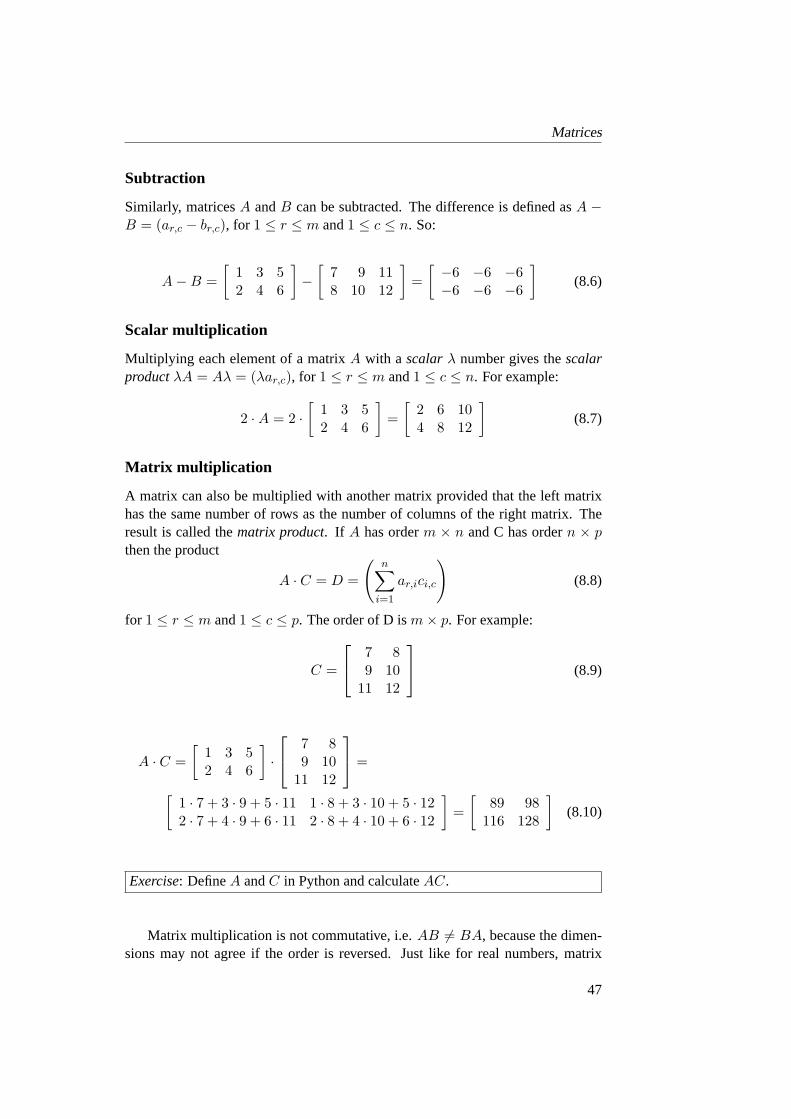
Matrix multiplication

A matrix can also be multiplied with another matrix provided that the left matrixhas the same number of rows as the number of columns of the right matrix. Theresult is called thematrix product. If A has orderm × n and C has ordern × pthen the product

A · C = D =

(

n∑

i=1

ar,ici,c

)

(8.8)

for 1 ≤ r ≤ m and1 ≤ c ≤ p. The order of D ism× p. For example:

C =

7 89 10

11 12

(8.9)

A · C =

[

1 3 52 4 6

]

·

7 89 10

11 12

=

[

1 · 7 + 3 · 9 + 5 · 11 1 · 8 + 3 · 10 + 5 · 122 · 7 + 4 · 9 + 6 · 11 2 · 8 + 4 · 10 + 6 · 12

]

=

[

89 98116 128

]

(8.10)

Exercise: DefineA andC in Python and calculateAC.

Matrix multiplication is not commutative, i.e.AB 6= BA, because the dimen-sions may not agree if the order is reversed. Just like for real numbers, matrix

47

Chapter 8

multiplication is both associative, i.e.(AB)C = A(BC) and distributive, i.e.(A+B)C = AC +BC andC(A+B) = CA+ CB.

The result of a multiplication of a matrixA by a zero matrixO isA ·O = O =0. Multiplying a matrixA with an identity matrixI givesA · I = A. For squarematrices it holds thatA · I = I ·A = A andA ·O = O ·A = O.

Note that matrix division is undefined. So ifA · C = D then there is no suchthing asC = D/A. If A andD are give,C can be found, however, by multiplyingD with the so-calledinverse of A (A has to be square). Before discussing thisconcept, it is necessary to introduce another matrix property, thedeterminant.

8.4 Determinant

Every square matrix has a real number associated with it which is called thede-terminant. The determinant of matrixA is denoted bydetA or sometimes|A|.It is not so easy to explain what a determinant is in words so let’s just considerits mathematical definition and start with the determinant of a2 × 2 matrix. It isdefined as the product of the elements on the principal diagonal minus the productof the elements off the principal diagonal:

det

[

a1,1 a1,2

a2,1 a2,2

]

= a1,1a2,2 − a1,2a2,1 (8.11)

For square matrices of size 3 and more, a technique calledLaplace expansioncan be used to determine the determinant. It is based on the expansion of a matrixin minors andcofactors.

Minor

Suppose we have square matrixA. For every elementar,c in A there exists aquantity calledminor which is the determinant of the matrix that results when therow r and columnc are deleted from the original matrix. For example:

A =

1 1 12 4 −33 6 −5

(8.12)

then fora1,1 the minorM1,1 is:

M1,1 = det

[

4 −36 −5

]

= 4 · −5 −−3 · 6 = −2 (8.13)

Cofactor

Thecofactor is theminor Mr,c multiplied by(−1)r+c:

Cr,c = (−1)r+cMr,c (8.14)

48

Matrices

whereCr,c is the cofactor. The factor(−1)r+c effectively determines the sign ofthe minor depending on its position within the matrix. So ifr + c is positive, thesign of the minor does not change. Ifr+c is negative the sign of the minor reverses.

Exercise: Calculate the cofactorsC1,1, C1,2 andC1,3.

With the minor and cofactor defined, the determinant of a matrix can be foundfrom:

detA =n∑

c=1

ar,cCr,c (8.15)

for any rowr. In words this formula reads: The determinant of a matrix is the sumof the product of the elements in a particular row multiplied by their cofactors. Forexample:

detA = det

1 1 12 4 −33 6 −5

= a1,1C1,1 + a1,2C1,2 + a1,3C1,3 (8.16)

Inserting the numbers gives:

detA = 1 · −2 + 1 · 1 + 1 · 0 = −1 (8.17)

Exercise: CalculatedetA by selectingr = 3.

The same approach can be applied by selecting a particular column rather thana row. The determinant is the calculated from:

detA =m∑

r=1

ar,cCr,c (8.18)

for any columnc.

Exercise: CalculatedetA by selectingc = 2.

For square matrices of size 4 and higher, the approach is the same. The workinvolved can be substantial: For a4 × 4 matrix, four cofactors must be calculated,each requiring three2× 2 determinants to be calculated, i.e. a total of twelve2× 2determinants. For any sizen the number of2 × 2 determinants to be calculatedis n!/2. In practice this number can be less if the matrix contains zero elements:Because the cofactor is multiplied with the value of the element, there is no need

49

Chapter 8

to calculate the cofactor if it is multiplied by a zero anyway. Consider a matrixZwhich contains 2 zero elements in columnc = 2:

Z =

6 4 0 28 0 2 46 0 4 2

18 4 6 2

(8.19)

Expanding along columnc = 2 will halve the number of calculations involvedsince there is no point in calculating the cofactorsC2,2 andC3,2 because these aremultiplied withz2,2 = 0 andz2,3 = 0.

Exercise: Use Python to calculate the determinant ofZ.

Transposing a square matrix does not change it determinant, i.e.detA =detAT . If any two rows or columns are interchanged the numerical value of thedeterminant remains the same but its sign changes. If a matrix is multiplied by ascalar, then the determinant is also multiplied by this scalar, i.e.detλA = λ detA.For matrix multiplication it holds that whenA andB are square and of the sameorder,detAB = detAdetB

8.5 Cramer’s rule

One application of determinants is the solution of a system of linear equations usingCramer’s rule. Suppose we have a system of 3 linear equations with 3 unknowns:

x1 + x2 + x3 = 92x1 + 4x2 − 3x3 = 13x1 + 6x2 − 5x3 = 0

(8.20)

which can be written in matrix form as (cf. Equation 8.8):

1 1 12 4 −33 6 −5

x1

x2

x3

=

910

(8.21)

or, withA,X andR representing the respective matrices:

AX = R (8.22)

Cramer’s rule states that the elements ofX can be found from:

xr =detAcdetA

(8.23)

50

Matrices

for 1 ≤ r ≤ m andc = r. Ac is the matrix that is obtained when columnc in A isreplaced by column vectorR. For example, to findx1, the first step is to calculatedetA1, which is:

detA1 = det

9 1 11 4 −30 6 −5

= −7 (8.24)

The determinant ofAwas calculated earlier (Equation 8.17). Inserting these valuesinto Equation 8.23 gives:

x1 =−7

−1= 7 (8.25)

Exercise: Apply Cramer’s rule to findx2 andx3.

The determinant of a matrix can be zero if an entire row is zero or if a row(or column) is a multiple of another row (or column). This also includes rows (orcolumns) which are the same (i.e. the multiplier is 1). If the determinant of a matrixis zero, it is called asingular matrix. SincedetA appears in the denominator ofEquation 8.23, Cramer’s rule can not be applied when a matrix is singular. Severalconditions may apply depending on the values of the determinants ofA andR.These are summarized in table 8.1.

A hydrological application of Cramer’s rule is in the derivation of the finiteelement approximation of the groundwater equation.

8.6 Inverse of a matrix

The inverse of a square matrixA is denoted byA−1 and is defined byAA−1 = I.The inverse can be used to solve a system of linear equations. The solutionof Xin Equation 8.22 is:

X = A−1R (8.26)

For a square matrixA the inverse can be found from:

A−1 =CT

detA(8.27)

Table 8.1: Possible solutions for systems of linear equations depending on thevalues ofdetA anddetR.

detR 6= 0 detR = 0

detA 6= 0 unique solution X = 0 (trivial solution)detA = 0 infinite number of solutions infinite number of solutions

if detAc = 0, 1 ≤ c ≤ m

51

Chapter 8

in which C is a matrix of cofactors ofA and its transposeCT is the so-calledadjugate of A. From Equation 8.27 it follows that the inverse can only exist ifdetA 6= 0. If this is the case thenA is called anon-singular matrix (as opposed toa singular matrix).

For matrixA in Equation 8.12,C is:

C =

−2 1 011 −8 −3−7 5 2

(8.28)

so:

A−1 =1

detACT =

1

−1

−2 11 −71 −8 50 −3 2

=

2 −11 7−1 8 −5

0 3 −2

(8.29)

Exercise: InsertA−1 andR (Equation 8.21) into Equation 8.26 to findX.

Exercise: Express the system of linear equations defined by Equation 7.15 inmatrix form, i.e.,Ah = R. Find h by calculatingA−1 and applying Equation8.26.

Obviously, calculating the inverse of a matrix by hand can be a lot of work andmistakes are easily made. Computers are much better at these sorts of calculationsthan humans.

Exercise: Use Python to calculateA−1 andA−1R = X.

52

References

Chiang, W. H., 2005. 3D-Groundwater modeling with PMWIN. Springer, BerlinHeidelberg, Germany.

Wang, H. F., Anderson, M. P. 1982. Introduction to Groundwater Modeling: FiniteDifference and Finite Element Methods. W. H. Freeman and Co, Gordonsville,Virginia, USA.

53