Groundwater Hydrology - Homework 2

Groundwater Hydrology - Homework 2

Due date: Nov. 26, 2012

1. In a confined, homogeneous and isotropic aquifer the following steady piezometric heads havebeen measured in three different wells A, B and C:

well A B CEast coord. (m) 0 300 0North coord.(m) 0 0 200head (m) +10 +11.5 +8.4

The aquifer is characterized by a thickness and a hydraulic conductivity equal to 20 m and 15 m/day,respectively.

Assuming a planar piezometric surface, determine:

a) direction and magnitude of the hydraulic gradient I;

b) total rate that flows through the aquifer (per unit length in the direction orthogonal to themaximum gradient);

c) Darcy’s velocity at point P=(100 m, 100 m).

Solution

a) The scenario is shown in the next plot:N

E

200 (+8.4 m)

(+10 m)

(+11.5 m)

300

θ

Since the piezometric surface is a plane, thus with a constant slope, we calculate the compo-nents of the gradient along East and North from the well couples A-B and A-C to obtain:

IEst =∂h

∂x=

11.5− 10

300= 5× 10−3

INord =∂h

∂y=

8.4− 10

200= −8× 10−3

1

Hence I =√I2Est + I2Nord = 9.43× 10−3 Direction θ is given by:

θ = arctan(IEstINord

)= 122◦ = 2.13rad

b) Total flow rate is:Q = k × b× I × 1 = 2.8 m3/day

c) Darcy’s velocity is:

v = k × I = 15× 9.43× 10−3 = 0.141 m/day

2

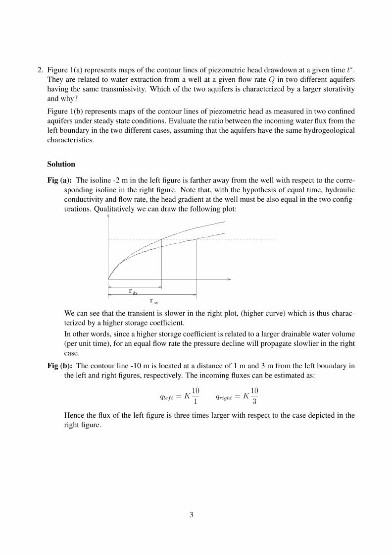
2. Figure 1(a) represents maps of the contour lines of piezometric head drawdown at a given time t∗.They are related to water extraction from a well at a given flow rate Q in two different aquifershaving the same transmissivity. Which of the two aquifers is characterized by a larger storativityand why?

Figure 1(b) represents maps of the contour lines of piezometric head as measured in two confinedaquifers under steady state conditions. Evaluate the ratio between the incoming water flux from theleft boundary in the two different cases, assuming that the aquifers have the same hydrogeologicalcharacteristics.

Solution

Fig (a): The isoline -2 m in the left figure is farther away from the well with respect to the corre-sponding isoline in the right figure. Note that, with the hypothesis of equal time, hydraulicconductivity and flow rate, the head gradient at the well must be also equal in the two config-urations. Qualitatively we can draw the following plot:

r

r

dx

sx

We can see that the transient is slower in the right plot, (higher curve) which is thus charac-terized by a higher storage coefficient.In other words, since a higher storage coefficient is related to a larger drainable water volume(per unit time), for an equal flow rate the pressure decline will propagate slowlier in the rightcase.

Fig (b): The contour line -10 m is located at a distance of 1 m and 3 m from the left boundary inthe left and right figures, respectively. The incoming fluxes can be estimated as:

qleft = K10

1qright = K

10

3

Hence the flux of the left figure is three times larger with respect to the case depicted in theright figure.

3

3. Figure 2 shows a contour representation of the piezometric surface for a confined aquifer discharg-ing into a river. Measurements of hydraulic heads made at 17 monitoring wells are shown in thefollowing Table:

Monitoring Piezometric Monitoring Piezometric Monitoring PiezometricWell Head (m asml) Well Head (m asml) Well Head (m asml)1 305.21 7 308.56 13 309.822 302.91 8 304.50 14 311.523 303.13 9 308.56 15 306.304 303.90 10 308.21 16 307.185 305.13 11 307.21 17 303.306 306.90 12 310.52

The aquifer has an average thickness of 16 m and is considered as homogeneous and isotropic,with a porosity of 0.29 and a hydraulic conductivity of 4.3 × 10−4 m/s. Assuming steady-stateconditions, estimate:

(a) the average hydraulic gradient in the aquifer;

(b) the rate of water discharge from the aquifer to the stream;

(c) the times it would take to a hypothetical tracer injected in Well # 16 to reach the river.

Solution

(a) There are many ways to solve this problem. One is to find an average gradient by fitting aplane through the data points by means of least square methods. This can be done by meansof the followin developments.Given N observations xi, yi, zi, i = 1, . . . , N , we try to approximate these data with a plane.The equation for a plane (linear function in 3D) is:

f(x, y) = z = ax+ by + c

We define the sum of squares as

S(a, b, c) =∑i=1

N [axi + byi + ci − zi]2

The determination of the coefficients a, b, c proceeds by minimizing this function with respectto these coefficients, i.e., by setting the partial derivatives to zero as follows:

∂S

∂a= 0 = 2

∑i=1

N [axi + byi + ci − zi]xi

∂S

∂b= 0 = 2

∑i=1

N [axi + byi + ci − zi] yi

∂S

∂c= 0 = 2

∑i=1

N [axi + byi + ci − zi]

4

This leads to the following linear system:∑Ni=1 x

2i

∑Ni=1 xiyi

∑Ni=1 xi∑N

i=1 xiyi∑Ni=1 y

2i

∑Ni=1 yi∑N

i=1 xi∑Ni=1 yi N

abc

=

∑Ni=1 xizi∑Ni=1 yizi∑Ni=1 zi

The following Matlab (Octave) code can be used for this:

#! /usr/bin/octave -qf

h_coord=load(’hw2-ex3.dat’);x=h_coord(:,1);y=h_coord(:,2);h=h_coord(:,3);

one=ones(n,1);

a11=dot(x,x);a22=dot(y,y);a33=n;a12=dot(x,y);a21=a12;a13=dot(x,one);a31=a13;a23=dot(y,one);a32=a23;

b1=dot(x,h);b2=dot(y,h);b3=dot(h,one);

A=[ a11, a12, a13; a21, a22, a23; a31, a32, a33]

b=[ b1; b2; b3]

A\b

Where the file hw2-ex3.dat is:

1026.99 878.496666667 305.211139.06466667 1454.15133333 302.911620.36266667 1820.54333333 303.132626.598 1775.092 303.901816.60533333 1494.906 305.131536.41933333 1168.87133333 306.902356.60066667 1061.89066667 308.562300.56333333 1601.886 304.50

5

1755.474 791.893333333 308.561403.968 679.819333333 308.21848.69 542.273333333 307.212224.14866667 476.047333333 310.522692.82333333 796.988 309.822458.486 633.970666667 311.522718.29533333 1377.73733333 306.32061.13133333 1230.00266667 307.182260.56333333 1945.092 303.30

The results from running the code is:

ans =

2.0986e-03-5.3675e-033.0881e+02

which gives an average gradient:

i =√

(−5.3675× 10−3)2 + (2.0986× 10−3)2 = 5.763× 10−3

Another way is to fit ∂h∂x

∂h∂y

as 1D linear functions using least squares (this is the less accurate,obviously, and if the data are clustered in some strange way (not this case) we can get largeerrors.Another way is to set up streamlines, as shown in the figure:

6

�

and calculate gradients with that. We obtain the following table:

Streamline l (m) ∆h (m) ∆h/l1 850 -6 −7.06× 10−3

2 1050 -6 −5.71× 10−3

3 1100 -6 −5.45× 10−3

4 1500 -8 −5.33× 10−3

5 1400 -8 −5.71× 10−3

Average gradient i = 5.86× 10−3

In this case, all the methods give similar results.

7

(b) From the last technique we obtain:

q = −b ·K · i16 = ·4.3× 10−4 · 5.86× 10−3 = 4× 10−3m3

s m= 3.48

m3

day m

We could have used the gradient as calculated from the 303 contour using again streamlines,and we would have obtained a slightly larger q.

(c) Along the streamline, the average gradient is i ≈ (307 − 302)/1100 = 0.0045. Then wehave:

vs = −Kωi = 6.74× 10−6 m/s

Thus the time for the particle to travel from well 16 to the stream is

t =d

vs= 1100/6.74× 10−6 = 1.63× 108 s = 5.2 years

8

4. Given the unconfined aquifer of Figure 3.

(a) Calculate the flow rate Qw in the well of Figure 3 (left) assuming steady state flow and radialsymmetry.

(b) Under the same assumptions, calculate the flow rate Qw in the well in Figure 3 (right).

Solution

(a) Assuming Dupuit-type flow, we can write the flow equation of the aquifer in steady stateconditions and homogeneous aquifer as:

1

r

d

dr

(rhdh

dr

)=

1

r

d

dr

(1

2rdh2

dr

)= 0

with boundary conditions:

Q = πrwKd(h2)

drat the well(r = rw)

h = H r = re

Itegrating this equation once we obtain:

r

2

dh2

dr= a

i.e.:d(h2) = a

dr

ror:

h2(r) = a ln r + b

From the first boundary condition, for r = rw:

Q = πKa ⇒ a =Q

πK

From the second conditions, for r = re:

H2 =Q

πKln re + b ⇒ b = H2 − Q

πKln re

The solution of the problem is then:

h2(r)−H2 =Q

πKlnr

re

Thus we can write:

Q = πK(h2(rw)−H2)/(lnrwre

) = 4748m3/day

9

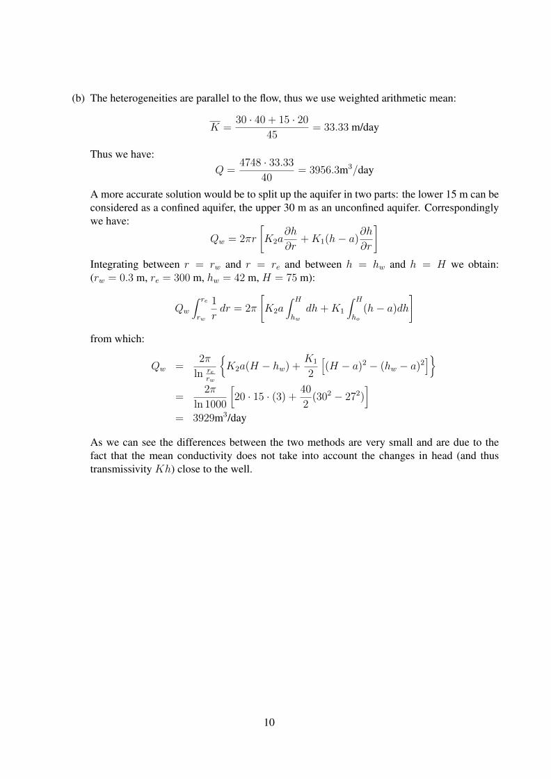
(b) The heterogeneities are parallel to the flow, thus we use weighted arithmetic mean:

K =30 · 40 + 15 · 20

45= 33.33 m/day

Thus we have:Q =

4748 · 33.33

40= 3956.3m3/day

A more accurate solution would be to split up the aquifer in two parts: the lower 15 m can beconsidered as a confined aquifer, the upper 30 m as an unconfined aquifer. Correspondinglywe have:

Qw = 2πr

[K2a

∂h

∂r+K1(h− a)

∂h

∂r

]Integrating between r = rw and r = re and between h = hw and h = H we obtain:(rw = 0.3 m, re = 300 m, hw = 42 m, H = 75 m):

Qw

∫ re

rw

1

rdr = 2π

[K2a

∫ H

hwdh+K1

∫ H

ho(h− a)dh

]

from which:

Qw =2π

ln rerw

{K2a(H − hw) +

K1

2

[(H − a)2 − (hw − a)2

]}

=2π

ln 1000

[20 · 15 · (3) +

40

2(302 − 272)

]= 3929m3/day

As we can see the differences between the two methods are very small and are due to thefact that the mean conductivity does not take into account the changes in head (and thustransmissivity Kh) close to the well.

10

5. Given the unconfined aquifer of Figure 4, assuming a uniform recharge flux e, calculate:

(a) the mathematical model governing this problem assuming that Dupuit assumption holds andthat the hydrogeological characteristics of the aquifer are constant (include initial and bound-ary conditions);

(b) the function h(x) describing the water table in steady state conditions. Assume: H1 = 20 m,H2 = 10 m, K = 5 × 10−3 m/s, recharge e = 7.2 mm/h, aquifer length L = L1 + L2 =2000 m.

(c) A ditch is to be excavated (along the y axis) in the mid section of the aquifer. What isthe maximum depth of the ditch so that no pumping is required for its excavation. (Makeapproprite assumptions if necessary.)

Solution

(a) Using Dupuit assumption the 1-D steady state equation of water flow in an unconfined aquifersubject to a recharge flux e is:

∂

∂x

(Kh

∂h

∂x

)= e

Integration of this equation leads to:

Kh∂h

∂x= −ex+ c′1

∂h2

∂x=

e

2Kx+ c1

h2(x) =e

Kx2 + c1x+ c2

(b) Using the boundary conditions h(0) = H1 and h(L) = H2, with L = L1 + L2, we obtain:

h(x) =

√e

K(x2 − Lx) +

H22 −H2

1

Lx+H2

1

where the convention is that a negative e corresponds to recharge. In our case we have:

h(x) =

√7.2 · 10−3

5× 10−3 · 3600(x2 − 2000x) +

102 − 202

2000x+ 202

h(x) =√−0.0004(x2 − 2000x)− 0.15x+ 400

(c) calculate the value of x at which the water table has a zero slope:

1

2h∂h

∂x=∂h2

∂x= 0 = −0.0008x+ 0.65

that yields: x∗ = 812.5 m. At that distance we have the maximum height of our water table,which we can set equal to the maximum excavation elevation required by the question:

h(812.5) =√−0.0004(812.52 − 2000 · 812.5)− 0.15 · 812.5 + 400 = 25.77 m

The maximum excavation depth is thus 30-25.77=4.23 m

11

6. Given the confined aquifer of Figure 5, determine the flow rate (per unit width in the directionorthogonal to the drawing) and draw an accurate plot of the behavior of the piezometric headbetween the two wells.

Solution The flowrate per unit width can be calculated using an average conductivity: since theheterogeneities are orthogonal to the flow, we need to use the harmonic mean:

Q = BKM∆h

L

where (L =∑Li):

L

KM

=L1

K1

+L2

K2

+L3

K3

=200

40+

800

10+

300

20= 13m/day

and thus:

Q = 50 ∗ 13 ∗ 4

1300= 2

m3

day m

The flowrate is constant in every section, so we have:

Q = Ti∆Hi

Lii = 1, 2, 3

from which:

∆H1 =QL1

T1=

2 ∗ 200

50 ∗ 40= 0.2m

∆H2 =QL2

T2=

2 ∗ 800

50 ∗ 10= 3.2m

∆H3 =QL3

T3=

2 ∗ 300

50 ∗ 20= 0.6m

12

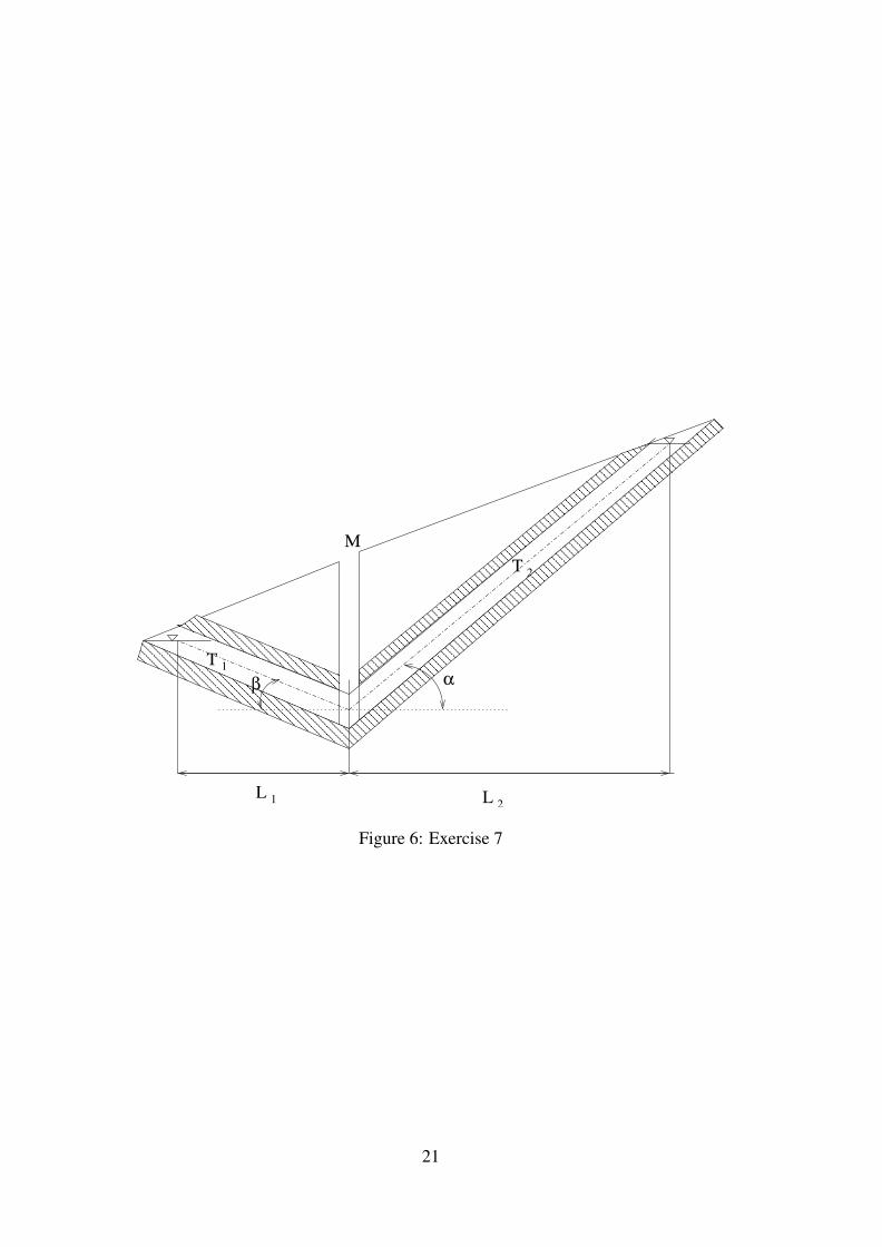
7. The aquifer system in Figure 6 is formed by two confined aquifers characterized by transmissivitiesT1 and T2, respectively. Water enters in the upper right portion of the system and exits as a springin the lower left. Determine the head in the observation well M and calculate the conditions underwhich well M is artesian (water flows naturally out of the well).

Solution

(a) This aquifer, being confined, can be treated as a planar aquifer with lengths equal to l1 =L1/ cos β and l2 = L2/ cosα. Then we can define two linear solutions in the two subdomainsand impose the compatibility conditions (we put the zero of the x-axis at point M):

h1(x) = a1x+ b1

h2(x) = a2x+ b2

h1(−l1) = H1

h2(l2) = H2

h1(0) = h2(0)(= HM which is unknown)

T1dh1dx|x=0 = T2

dh2dx|x=0

From the last equations, and noting that for a linear function the gradients are constant andcan be calculated using H1, HM , and H2, we can write:

T1dh1dx

= T1HM −H1

l1= T2

dh2dx

= T2H2 −HM

l2

from which we obtain:Hm =

T1l2H1 + T2l1H2

T1l2 + T2l2Now, since L1 = l1 cos β and L2 = l2 cosα, we also have that H1 = L1 tan β and H2 =L2 tanα. Thus we can write:

Hm =T1 sin β + T2 sinαT1 cosβL1

+ T2 cosαL2

(b) The top of well shown in the Figure (point M) is at an height given by the linear interpolationbetween H1 and H2, i.e.,

Hwell =H2 −H1

L1 + L2

L1 +H1

To calculate the conditions for the aquifer for beeing artesian, we impose that HM > Hwell.The limiting condition is when:

L2H1 + L1H2

L1 + L2

=T1l2H1 + T2l1H2

T1l2 + T2l2

which is verified for example when:

T2l1 = L1

T1l2 = L2

13

8. Figure 7 reports two different configurations of wells and pizeometer in a confined aquifer, char-acterized by a hydraulic conductivity K = 10 m/day, an elastic storage coefficient Ss = 10−5 m−1

and a thicknessB=10 m. From the wells, water is extracted at the following rates: Q1 = 15 m3/dayfor 50 days; Q2 = 10 m3/day for 20 days; Q2 = 20 m3/day for the next 30 days; Q3 = 20 m3/dayfor 50 days. Calculate the drawdown in the piezometer W at t = 50 days for the two distinctconfigurations (a) and (b).

Solution

T = 100m2/day S = 10−4

a)

up1 =4Tt

r2S=

4 · 100 · 50

1002 · 10−4= 0.2× 105 > 100 apply Cooper-Jacob

∆hp1 =Q1

4πTln(

2.25Tt

r2S

)= 0.111 m

up2 =4Tt

r2S=

4 · 100 · 20

702 · 10−4= 0.167× 105 > 100 apply Cooper-Jacob

∆hp2,50days = ∆hQ2A,50days + ∆hQ2B ,30days; Q2A = 10m3/day;Q2B = 20− 10 = 10m3/day;

t2A = 50day; t2B = 30day

=Q2,A

4πTln(

2.25Tt2Ar2S

)+Q2,B

4πTln(

2.25Tt2Br2S

)=

= 0.080 + 0.076 = 0.156m

∆htot = 0.111 + 0.156 = 0.267m

b)

u =4Tt

r2S= 8.89× 103 > 100 apply Cooper-Jacob

∆h =Q3

4πTln(

2.25Tt

r2S

)= 0.136 m

14

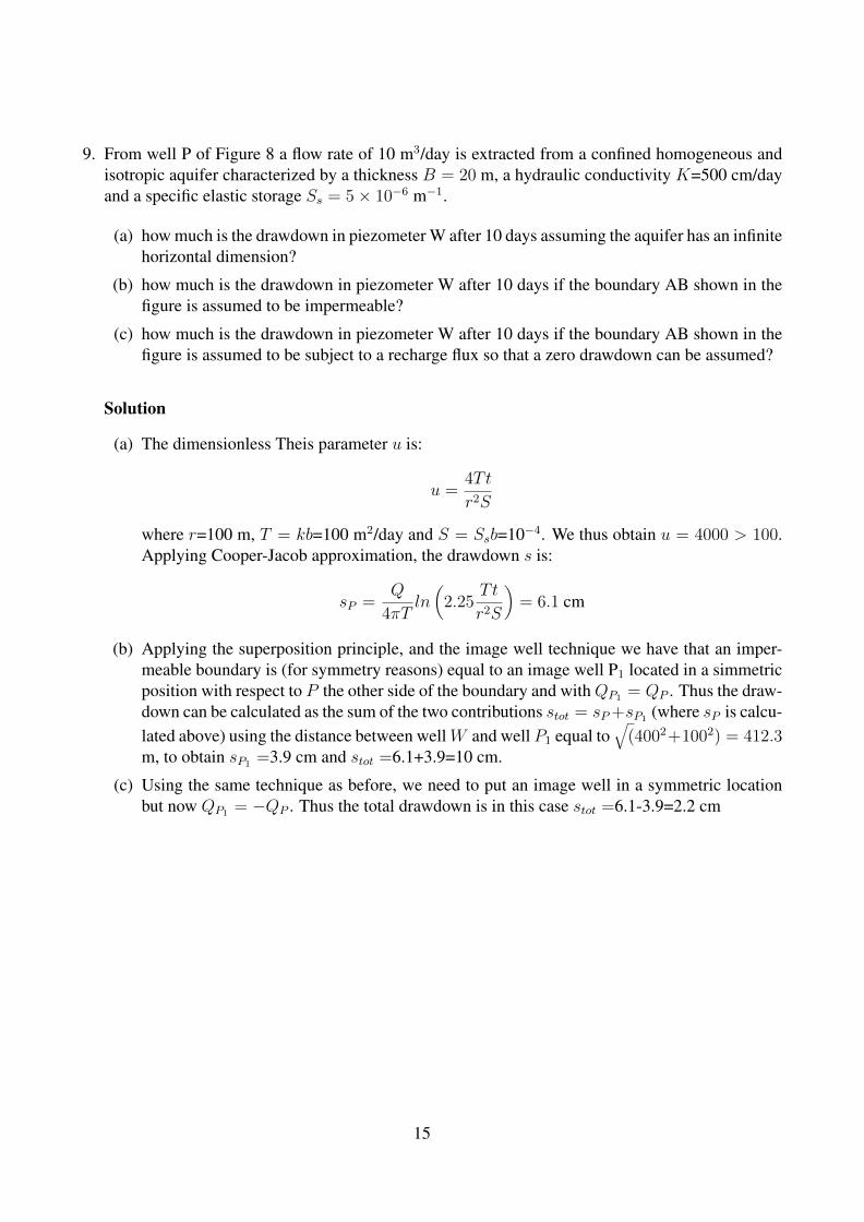
9. From well P of Figure 8 a flow rate of 10 m3/day is extracted from a confined homogeneous andisotropic aquifer characterized by a thickness B = 20 m, a hydraulic conductivity K=500 cm/dayand a specific elastic storage Ss = 5× 10−6 m−1.

(a) how much is the drawdown in piezometer W after 10 days assuming the aquifer has an infinitehorizontal dimension?

(b) how much is the drawdown in piezometer W after 10 days if the boundary AB shown in thefigure is assumed to be impermeable?

(c) how much is the drawdown in piezometer W after 10 days if the boundary AB shown in thefigure is assumed to be subject to a recharge flux so that a zero drawdown can be assumed?

Solution

(a) The dimensionless Theis parameter u is:

u =4Tt

r2S

where r=100 m, T = kb=100 m2/day and S = Ssb=10−4. We thus obtain u = 4000 > 100.Applying Cooper-Jacob approximation, the drawdown s is:

sP =Q

4πTln(

2.25Tt

r2S

)= 6.1 cm

(b) Applying the superposition principle, and the image well technique we have that an imper-meable boundary is (for symmetry reasons) equal to an image well P1 located in a simmetricposition with respect to P the other side of the boundary and withQP1 = QP . Thus the draw-down can be calculated as the sum of the two contributions stot = sP +sP1 (where sP is calcu-lated above) using the distance between wellW and well P1 equal to

√(4002+1002) = 412.3

m, to obtain sP1 =3.9 cm and stot =6.1+3.9=10 cm.

(c) Using the same technique as before, we need to put an image well in a symmetric locationbut now QP1 = −QP . Thus the total drawdown is in this case stot =6.1-3.9=2.2 cm

15

−2 m

−1 m

−2 m

−1 m

Q Q

−10 m −5 m 0 m −5 m−10 m

(a)

(b)

0 m

0 m

41 5 4 3 5 6

Figure 1: Exercise 2.

16

Figure 2: Exercise 3

17

rw

h =42 mw

K = 40 m/g1

=0.3 m

30 m

75 m

90 m

Q w

re =300 m

3 m

h

H

rw

h =42 mw

=0.3 m

30 m

45 m

75 m

90 m

Q w

re =300 m

K = 40 m/g1

3 m

a=15m

b=30m

h

H

K = 20 m/g2

Figure 3: Exercise 4. the unit m/g is in Italian; it means m/day.

18

H

Hh

H

L L

1

2

21

x

z

e

30 m


19

+8.6 m

+4.6 m

K =20m/g K =10 m/g K =40 m/g123

300 m 800 m 200 m

50 m

Figure 5: Exercise 6; the unit m/g is in Italian; it means m/day.

20

L1

T1

T2

��

��

��

��

��

��

αβ

Μ

L2


21

W P

Q

3

3

WP P

QQ

1 2

1 2

(a) (b)

70 m100 m 150 m


22

��

��

��

��

��

P W

100 m

A B

200 m

Figure 8: Exercise 9.

23

Groundwater Hydrology - Homework 2

Documents

Transcript of Groundwater Hydrology - Homework 2