Groundwater Flow Modeling and Aquifer vulnerability ... · (3) Estimation of Dynamic Groundwater...
173
Groundwater Flow Modelling and Aquifer vulnerability assessment studies in Yamuna–Krishni Sub-basin, Muzaffarnagar District (Project No.23/36/2004-R&D) Completion Report Submitted to Indian National Committee on Ground Water Central Ground Water Board (CGWB) Ministry of Water Resources (Govt. of India) By Dr. Rashid Umar Principal Investigator Department of Geology Aligarh Muslim University Aligarh (U.P.) - 202002
Transcript of Groundwater Flow Modeling and Aquifer vulnerability ... · (3) Estimation of Dynamic Groundwater...
Groundwater Flow Modelling and Aquifer vulnerability assessment studies in Yamuna–Krishni Sub-basin,
Muzaffarnagar District
(Project No.23/36/2004-R&D)
Completion Report
Submitted to
Indian National Committee on Ground Water Central Ground Water Board (CGWB)
Ministry of Water Resources (Govt. of India)
By
Dr. Rashid Umar Principal Investigator
Department of Geology Aligarh Muslim University
Aligarh (U.P.) - 202002
CONTENTS
I List of Figures i-iii II List of Tables iv III List of Appendices v IV List of Plates vi
1. Name and address of the Institute 1 2. Name and addresses of the PI and other investigators 1 3 Title of the scheme 1 4. Financial details 1 5. Original objectives and methodology as in the sanctioned proposal 2-4 6. Any changes in the objectives during the operation of the scheme 4 7. All data collected and used in the analysis with sources of data 4 8. Methodology actually followed. (observations, analysis, results and inferences) 4-111 (1) The Study Area 7-17
(2) Hydrogeology 18-42
(3) Estimation of Dynamic Groundwater Resource 43-54
(4) Groundwater Flow Modelling 55-75
(5) Groundwater Vulnerability Assessment 76-85
(6) Hydrogeochemistry 86-106
(7) Project findings 107-111
9. Conclusions / Recommendations 112-115 10. How do the conclusions / recommendations compare with current thinking 115-116 11. Field tests conducted 116
12. Software generated, if any 116 13. Possibilities of any patents / copyrights. If so, then action taken in this regard 116 14. Suggestions for further work 116 Publications 117 References 118-123 Appendices
i
LIST OF FIGURES
Fig No. Title Page No.
Fig.1.1 Location map of the study area 7 Fig.1.2 Digital elevation model (DEM) of Yamuna-Krishni sub-basin 10 Fig.1.3a Landuse/Landcover pattern in the study area (1971) 11 Fig.1.3b Landuse/Landcover pattern in the study area (2002) 12 Fig.1.4 Block wise water utilization pattern. 13 Fig.1.5a Yearly rainfall at Kairana raingauge station(1990-2007) 13 Fig.1.5b Yearly rainfall at Shamli raingauge station(1990-2007) 14 Fig.1.6 Isohyetal map showing distribution of average annual rainfall. 15 Fig.1.7 Soil map of the study area 16 Fig.1.8 Map of the Ganga Plain showing sub-surface basement high and thickness of the foreland sediment (in kilometers) Compiled from various sources, namely Agarwal 1977, Karunakaran and Ranga Rao 1979 and Singh 2004 17 Fig.2.1 Base map of Yamuna-Krishni sub-basin 19 Fig.2.2 Fence diagram showing aquifer disposition in Yamuna-Krishni sub-basin 20 Fig.2.3 Hydrogeological cross section along line A-B 21 Fig.2.4 Hydrogeological cross section along line C-D 21 Fig.2.5 Hydrogeological cross section along line E-F 22 Fig.2.6 Sand percent map of the study area 23 Fig.2.7 Pre-monsoon depth to water level map (June 2006) 25 Fig.2.8 Post-monsoon depth to water level map (Nov 2006) 25 Fig.2.9a Water level fluctuation map (2006) 27 Fig.2.9b Water level fluctuation map (2007) 27 Fig.2.10 3-D water table contour map 29 Fig.2.11 Pre-monsoon water table contour map (June 2006) 30 Fig.2.12 Post-monsoon water table contour map (Nov 2006) 30 Fig.2.13a Long term water level fluctuation trends at Thanabhawan and Jalalabad 32 Fig.2.13b Long term water level fluctuation trends at Shamli and Titoli 33 Fig.2.13c Long term water level fluctuation trends at Bhabhisa and Gangeru 33 Fig.2.13d Long term water level fluctuation trends at Garhi Abdullah and Toda 33 Fig.2.13e Long term water level fluctuation trends at Bhoora and Kandela 34 Fig.2.13f Long term water level fluctuation trends at Kairana and Khurgyan 34 Fig.2.13g Long term water level fluctuation trends at Kandhala and Mawi 34 Fig.2.14a Bimonthly water level fluctuation trends at Choutra, Chandelmal and Goharni 35 Fig.2.14b Bimonthly water level fluctuation trends at Khurgyan, Saiupat and Malakpur 35 Fig.2.14c Bimonthly water level fluctuation trends at Bunta, Chausana and Kairana 36 Fig.2.14d Bimonthly water level fluctuation trends at Garhi Pukhta, Todda and Lilaun 36
ii
Fig.2.14e Bimonthly water level fluctuation trends at Harhar Fatehpur and Bhanera 36 Fig.2.15a Temporal variability of monthly rainfall and water level at Kairana 37 Fig.2.15b Temporal variability of monthly rainfall and water level at Shamli 38 Fig.2.16 Logan’s Isopermeability map 40 Fig.3.1 Command and Non-command area 44 Fig.3.2 Horizontal flows across the Yamuna-Krishni sub-basin 50 Fig.3.3a Hydrograph showing significant decline in command area 53 Fig.3.3b Hydrograph showing significant decline in non-command area 54 Fig.4.1a Zone wise permeability distribution in first and third layer 58 Fig.4.1b Zone wise permeability distribution in second layer 58 Fig.4.2 Zone wise recharge distribution in Yamuna-Krishni model 59 Fig.4.3 Simulated groundwater pumping centers in Yamuna-Krishni Model 60 Fig.4.4 Map showing boundary condition in the study area 61 Fig.4.5 Grid pattern and location of observation wells in Yamuna- Krishni model 63 Fig.4.6a Hydrogeological cross section along row 9 showing three layer system 63 Fig.4.6b Hydrogeological cross section along row 25 showing three layer system 63 Fig.4.7a Observed water table contour map (Nov 2006) 65 Fig.4.7b Simulated water table contour map (Nov 2006) 65 Fig.4.8 Calculated versus observed heads (Nov 2006) 66 Fig.4.9 Calculated versus observed heads (June 1999-June 2007) 68 Fig.4.10a Observed and simulated heads at Kairana, Titoli and Thanabhawan 68 Fig.4.10b Observed and simulated heads at Shamli and Khurgyan 69 Fig.4.10c Observed and simulated heads at Bhoora and Todda 69 Fig.4.10d Observed and simulated heads at Jalalabad and Kandela 70 Fig.4.11a Drawdown in prediction scenario 1 73 Fig.4.11b Drawdown in prediction scenario 2 74 Fig.4.11c Drawdown in prediction scenario 3 75 Fig.5.1 Procedure for the construction of the Aquifer vulnerability map 78 Fig.5.2 Depth to water level map (Nov 2007) 78 Fig.5.3 Soil map of the study area 80 Fig.5.4 Zone wise hydraulic conductivity distribution 82 Fig.5.5 Aquifer vulnerability map of Yamuna-Krishni sub-basin 84 Fig.6.1 Sampling location map of the study area 87 Fig.6.2 TDS distribution map in the study area 90 Fig.6.3 Relative abundances of Alkali’s over Ca+Mg 93 Fig.6.4 Relative abundances of HCO3 and Cl+SO4 93 Fig.6.5 Bonding affinity between Alkali’s and Cl 94 Fig.6.6 Bonding affinity between Ca+Mg and HCO3 94 Fig.6.7 Bonding affinity between Ca and SO4 95 Fig.6.8a Chemical classification of groundwater based on Piper diagram (November 2005) 96
iii
Fig.6.8b Chemical classification of groundwater based on Piper diagram (June 2006) 96 Fig.6.9a Langelier and Ludwig diagram of post-monsoon samples (Nov 2005) 98 Fig.6.9b Langelier and Ludwig diagram of pre-monsoon samples (June 2006) 98 Fig.6.10a Salinity and Alkalinity hazards of Irrigation water in US Salinity diagram (Nov 2005) 104 Fig.6.10b Salinity and Alkalinity hazards of Irrigation water in US Salinity diagram (June 2006) 104
iv
LIST OF TABLES
Table No. Title Page No.
Table 1.1 Change in LULC pattern in the study area 11 Table 1.2 Results of statistical analysis of annual rainfall data 14 Table 1.3 Probable Geological succession in the study area 17 Table 2.1 Effective Grain size and Uniformity coefficient 23 Table 2.2 Average annual decline during (1999-2007) in command area 32 Table 2.3 Average annual decline during (1999-2007) in non-command area 32 Table 2.4 Results of Laboratory Hydraulic Conductivity (m/day) 41 Table 2.5 Results of the long duration Pump test 41 Table 2.6 Results of the short duration Pump test 42 Table 3.1 Non-monsoon rainfall recharge 46 Table 3.2 Seasonal (crop wise) irrigation return flow in command area 47 Table 3.3 Seasonal (crop wise) irrigation return flow in non-command area 47 Table 3.4 Recharge through Canal seepage 48 Table 3.5 Recharge through surface water irrigation 48 Table 3.6 Subsurface horizontal inflows across the sub-basin 49 Table 3.7 River aquifer interaction 49 Table 3.8 Annual groundwater recharge in the study area (Mcum) 49 Table 3.9 Borewells census in the study area 50 Table 3.10 Groundwater draft through pumpage (Mcum) 51 Table 3.11 Discharge through EVAP in the study area 51 Table 3.12 Subsurface horizontal outflows (Mcum) 51 Table 3.13 Total discharge in the study area (Mcum) 52 Table 3.14 Stages of groundwater development (June 2006 to May 2007) 52 Table 3.15 Stages of groundwater development (June 2007 to May 2008) 53 Table 4.1 River aquifer interaction 72 Table 4.2 Components of groundwater balance using MODFLOW 72 Table 5.1 Assigned weight for DRASTIC parameter (after Aller et al 1987) 79 Table 5.2 Hydraulic conductivity ranges and their ratings 81 Table 5.3 Land use categories ratings 82 Table 6.1 Hardness classification of water 89 Table 6.2 Range of concentration of various major and Trace elements in Shallow groundwater Samples and their comparison with W.H.O. (1993) and B.I.S. (1991) Drinking Water Standards 102 Table 6.3 Quality classification of Irrigation water (after USSL 1954) 103 Table 6.4 Quality of groundwater based on residual sodium carbonate 105
v
LIST OF APPENDICES
Appendix Title Page No.
I A Statistical analysis of Rainfall data at Kairana Raingauge Station i I B Statistical analysis of Rainfall data at Shamli Raingauge Station i II Latitudes and Longitudes and their corresponding x and y of monitoring wells ii-iii III Lithological Logs of Boreholes iv-xii IV A Well inventoried for water level monitoring xiii-xiv IV B Water level monitoring data (June 2006) xiv-xv IV C Water level monitoring data (November 2006) xv-xvi IV D Water level monitoring data (June 2007) xvii-xviii IV E Water level monitoring data (November 2007) xviii-xix V A Well hydrographs data in non-command area xix V B Well hydrographs data in command area xx VI Bimonthly water level monitoring data xx VII A Results of chemical analysis (November 2005) xxi-xxii VIIB Results of chemical analysis (June 2006) xxii-xxiii VIIC Results of chemical analysis (November 2006) xxiv VIID Results of chemical analysis (June 2007) xxv-xxvi VIII A Results of chemical analysis of river water samples (November 2005) xxvi VIIIB Results of chemical analysis of river water samples (June 2007) xxvii VIII C Results of chemical analysis of Nala/Drain samples
(June 2007) xxvii IX A Trace elements analysis of groundwater samples (June 2006) xxviii IX B Repeat Analysis of Trace elements of groundwater samples (June 2007) xxix IX C Trace elements analysis of surface water sample (June 2007) xxix X A Results of chemical analysis of effluent samples
(Results in mg/l) xxx X B Analysis of trace elements of effluent samples in mg/l xxx XI A Recharge applied for each stress period xxxi XI B Data of pumping rate applied for each stress period xxxii XI C Initial and final head of the study area xxxii-xxxiii
vi
LIST OF PLATES
Plate 1a Yamuna River at Chautra Plate 1b Base flow of Yamuna River at Chautra Plate 1c Yamuna River at Mawi Plate 2 Krishni River at Banat Plate 3 Saline soil at location Mansura Plate 4a, b&c Water level monitoring during pre-and post monsoon Plate 5 Collection of Sand material Plate 6 Groundwater discharge in the study area Plate 7a Surface water sample collection from river Yamuna Plate 7b Surface water sample collection from river Krishni Plate 8a Surface water sample collection from Kandela Drain Plate 8b Surface water sample collection from Sikka Nala Plate 9 Shamli Paper Mill at Sikka
1
1. Name and address of the Institute:
Department of Geology
Aligarh Muslim University, Aligarh
Pin- 202002
2. Name and addresses of the PI and other investigators.
Name and address of the PI:
Dr. Rashid Umar
Senior Lecturer,
Department of Geology,
Aligarh Muslim University, Aligarh.
Contact no: 0571-2700615
Email: [email protected]
3. Title of the scheme:
“Groundwater Flow Modelling and Aquifer vulnerability Assessment Studies in
Yamuna-Krishni Sub-basin, Muzaffarnagar District”
4. Financial details:
Sanctioned
cost
Amount
released
Expenditure Unspent
balance
Return of
unspent balance
13,82,000 11,18,900 10,43,928 74,972 CR ------
2
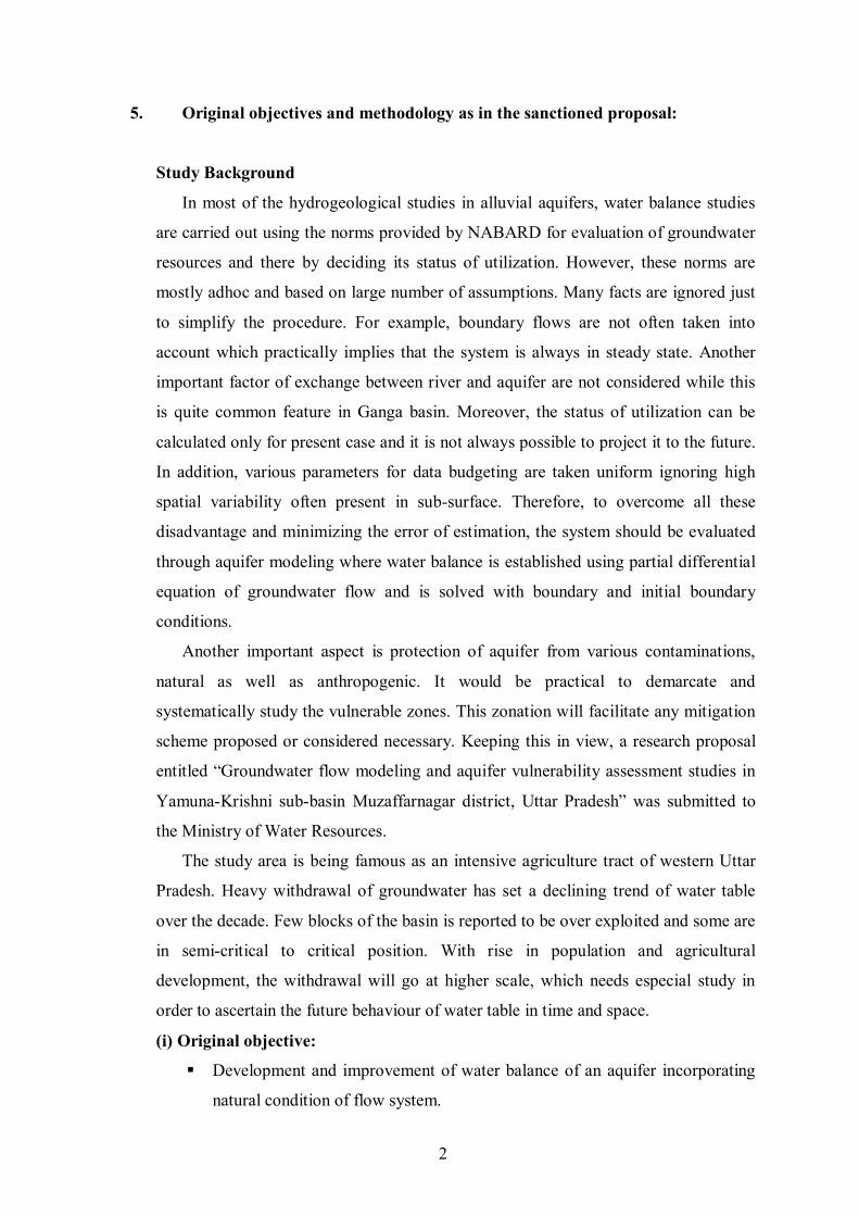
5. Original objectives and methodology as in the sanctioned proposal:
Study Background
In most of the hydrogeological studies in alluvial aquifers, water balance studies
are carried out using the norms provided by NABARD for evaluation of groundwater
resources and there by deciding its status of utilization. However, these norms are
mostly adhoc and based on large number of assumptions. Many facts are ignored just
to simplify the procedure. For example, boundary flows are not often taken into
account which practically implies that the system is always in steady state. Another
important factor of exchange between river and aquifer are not considered while this
is quite common feature in Ganga basin. Moreover, the status of utilization can be
calculated only for present case and it is not always possible to project it to the future.
In addition, various parameters for data budgeting are taken uniform ignoring high
spatial variability often present in sub-surface. Therefore, to overcome all these
disadvantage and minimizing the error of estimation, the system should be evaluated
through aquifer modeling where water balance is established using partial differential
equation of groundwater flow and is solved with boundary and initial boundary
conditions.
Another important aspect is protection of aquifer from various contaminations,
natural as well as anthropogenic. It would be practical to demarcate and
systematically study the vulnerable zones. This zonation will facilitate any mitigation
scheme proposed or considered necessary. Keeping this in view, a research proposal
entitled “Groundwater flow modeling and aquifer vulnerability assessment studies in
Yamuna-Krishni sub-basin Muzaffarnagar district, Uttar Pradesh” was submitted to
the Ministry of Water Resources.
The study area is being famous as an intensive agriculture tract of western Uttar
Pradesh. Heavy withdrawal of groundwater has set a declining trend of water table
over the decade. Few blocks of the basin is reported to be over exploited and some are
in semi-critical to critical position. With rise in population and agricultural
development, the withdrawal will go at higher scale, which needs especial study in
order to ascertain the future behaviour of water table in time and space.
(i) Original objective:
Development and improvement of water balance of an aquifer incorporating
natural condition of flow system.
3
Demarcations of aquifer zone vulnerable to contaminations and feasibility
study of its mitigation.
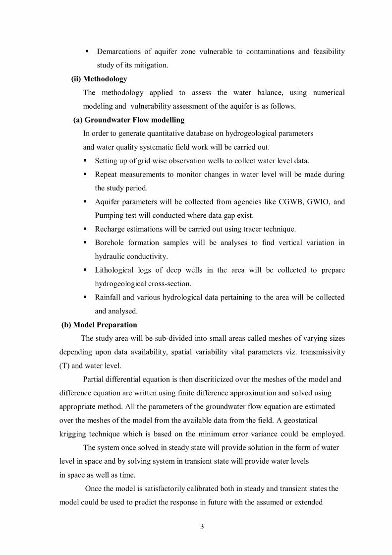
(ii) Methodology
The methodology applied to assess the water balance, using numerical
modeling and vulnerability assessment of the aquifer is as follows.
(a) Groundwater Flow modelling
In order to generate quantitative database on hydrogeological parameters
and water quality systematic field work will be carried out.
Setting up of grid wise observation wells to collect water level data.
Repeat measurements to monitor changes in water level will be made during
the study period.
Aquifer parameters will be collected from agencies like CGWB, GWIO, and
Pumping test will conducted where data gap exist.
Recharge estimations will be carried out using tracer technique.
Borehole formation samples will be analyses to find vertical variation in
hydraulic conductivity.
Lithological logs of deep wells in the area will be collected to prepare
hydrogeological cross-section.
Rainfall and various hydrological data pertaining to the area will be collected
and analysed.
(b) Model Preparation
The study area will be sub-divided into small areas called meshes of varying sizes
depending upon data availability, spatial variability vital parameters viz. transmissivity
(T) and water level.
Partial differential equation is then discriticized over the meshes of the model and
difference equation are written using finite difference approximation and solved using
appropriate method. All the parameters of the groundwater flow equation are estimated
over the meshes of the model from the available data from the field. A geostatical
krigging technique which is based on the minimum error variance could be employed.
The system once solved in steady state will provide solution in the form of water
level in space and by solving system in transient state will provide water levels
in space as well as time.
Once the model is satisfactorily calibrated both in steady and transient states the
model could be used to predict the response in future with the assumed or extended
4
values of input mainly the demand and rainfall recharge.
(c) Aquifer vulnerability
A detailed soil and hydrogeological investigation will be carried out by
interpreting a
range of soil properties such as texture, structure, thickness organic carbon content, clay
mineral content, permeability, geologic and hydrogeologic criteria to zone land according
to its intrinsic characteristics. Considering the above facts aquifer vulnerability map will
be prepared.
6. Any changes in the objectives during the operation of the scheme. - No
7. All data collected and used in the analysis with sources of data
All the data generated and collected are listed in appendices (please see- Page No.
i to xxxiii).
8. Methodology actually followed. (observations, analysis, results and
inferences).
(i) Methodology
In order to generate quantitative data base to infer hydrogeology, groundwater
resource evaluation and chemical characteristics of Yamuna-Krishni sub-basin,
systematic groundwater surveys were carried out supported by laboratory investigations.
The literature pertaining to study area was collected and background information
on state-of-the-art was generated.
Toposheets of the study area were used to generate base map for the field survey.
Rainfall and various other hydrological and hydrogeological data pertaining to the
area were collected. The rainfall data were statistically analysed and the mean,
standard deviation, coefficient of variation were calculated.
A Landuse and Landcover map for the area was generated, using the remote
sensing data from IRS-1B LISS-II and IRS-1D, LISS-III. A change detection
analysis in Landuse and Landcover using two time period data is also attempted.
Initially 71 wells were selected for water level monitoring in November 2005.
Later it was reduced to 60 wells and monitoring were carried out in these wells in
2006, 2007 respectively.
5
Coordinates of the borewells were taken using GPS.
Repeat measurements to monitor the changes in water level, for pre and post
monsoon were carried out in year 2006 and 2007 in all the monitoring wells.
Bimonthly monitoring were also carried out from February 2007 to November
2008.
The water level data of monitoring wells were processed and various maps like
depth to water maps, water table contour maps and water level fluctuation maps
were prepared.
Historical water level data of 14 hydrograph stations monitored by Central
Ground Water Board and State Groundwater Department was utilized to prepare
hydrographs to infer long term water level trends.
Lithologs of deep tube wells were collected to prepare cross-sections and fence
diagram.
Sand samples were collected from varying depths of granular zones and were
utilized for permeability estimation in the Laboratory using Permeameter.
The sand samples were also mechanically analysed for grain size analysis and
parameters like effective grain size and uniformity coefficient were determined.
Groundwater Budget were prepared for June 2006 to May 2007 and June 2007 to
May 2008 using guidelines provided by Groundwater Estimation Committee
(GEC) 1997.
Groundwater flow model was prepared using software Visual MODFLOW
Version 4.1 Pro.
Steady state model was prepared for November 2006 and transient state model
was prepared from June 1999 to November 2007.
Sustainability of groundwater regime was attempted for next 8 years under
variable stresses.
Classification of aquifer vulnerability to contamination is also carried out using
modified DRASTIC model.
In all, 144 groundwater samples were collected for physico-chemical analysis in
four successive season’s viz. post-monsoon and pre-monsoon period
corresponding November 2005, June 2006, November 2006 and June 2007
respectively.
6
Twenty six groundwater samples in June 2006 were analysed for trace elements
using ICPMS.
Fourteen surface water samples were collected from river Yamuna and Krishni
for major ion analysis. In addition 4 drains and two sugar factory effluent samples
were also collected for similar analyses.
Six surface water samples were also analysed for trace element.
Groundwater of the study area was classified into different chemical groups on
the basis of major ions concentrations.
Various mechanisms were identified and presented, which seem responsible for
alteration in groundwater chemistry.
Concurrence and synthesis of hydrogeological, hydrometeorological and hydro-
chemical data was attempted to generate the model for groundwater regime of
Yamuna – Krishni sub-basin presented in the present research work.
(ii) The work carried out and data generated are described and discussed
under following chapters.
(1) The Study Area
(2) Hydrogeology
(3) Estimation of Dynamic Groundwater Resource
(4) Groundwater Flow Modelling
(5) Groundwater Vulnerability Assessment
(6) Hydrogeochemistry
(7) Project findings
7
1 - THE STUDY AREA
1.1 Location and Accessibility
Muzaffarnagar is an important district in western Uttar Pradesh and the town
Muzaffarnagar is the district Headquarter. It lies in the interfluves of Ganga and Yamuna
rivers in the western most part of the Uttar Pradesh.
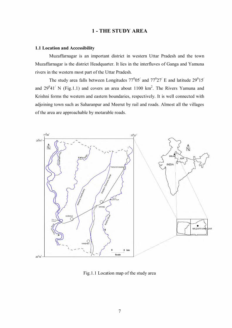
The study area falls between Longitudes 77005/ and 77027/ E and latitude 29015/
and 29041/ N (Fig.1.1) and covers an area about 1100 km2. The Rivers Yamuna and
Krishni forms the western and eastern boundaries, respectively. It is well connected with
adjoining town such as Saharanpur and Meerut by rail and roads. Almost all the villages
of the area are approachable by motarable roads.
Fig.1.1 Location map of the study area
8
1.2 Climate
The climate of the area is characterized by general dryness except during the
brief span of monsoon season. It has a hot summer and a cold winter. The year is
divided into the four seasons. The period from the middle of November to about the
ends of February is the cold season. The hot season which follows, continues up to the
end of June. The rainy season spans over the period of mid June to September. The
post-monsoon or the pre-winter extending from mid September to mid November
follows this. The highest temperature, reaching to 450C is generally recorded during
the month of June. The lowest temperature of about 40C is recorded during the month
of January. The average mean daily temperature of the area ranges from 20oC to 32oC.
Winds are generally light and only a little strong in the summer and monsoon
seasons. During October and April, they are mostly westerly or northwesterly. From May,
they become easterly and during the southwest monsoon season, they are predominantly
easterly or southeasterly.
1.3 Physiography and Drainage
District Muzaffarnagar is rectangular in shape and it is situated between the
district of Saharanpur on the north, Meerut and Baghpat on the south, and is bounded by
the Ganga on the east and the Yamuna on the west. The main rivers, the Ganga, the Kali,
the Hindon and the Yamuna have played an important role in carving the topography of
the district and divide it into four distinct tracts (Nevill, 1903, Varun, 1980) i.e. (i) the
Ganga Khadir (ii) upland upto Kali Nadi (iii) the Kali Hindon doab and (iv) the Hindon
Yamuna doab. The study area Krishni-Yamuna sub basin is a part of Hindon-Yamuna
doab.
The river Yamuna, which forms the western boundary of the district, flows in
an irregular course from north to south with uncertain and not well-defined channels
(Plate-1a, b & c). The rivers command a large tract of low-lying area of newer
alluvium, which is locally known as Khadir. The river krishni forms the eastern
boundary of the area. Near the river Krishni there is as usual, much poor soil and low
land areas are well adapted for rice cultivation. Krishni flows in a well-defined
channel (Plate-2), and the Khadir is small as compared to Yamuna.
The central upland is somewhat like an elevated plateau. Near Yamuna river
and the Katha drain the land are generally affected by saline soil. The villages lying
9
along the Katha on both sides have suffered largely from the increased volume of the
floods in this river, which now receives the contents of several drainage.
The eastern yamuna canal flows through water divide from north to south. The
low grounds along the canal have saline soil, which has thrown considerable area out
of cultivation (Plate-3). The soil is much less sandy than in and around the Yamuna
canal tract.
The drainage of the study area is mainly controlled by the two rivers i.e.
Krishni and Yamuna, which are flowing from north to south. Both the rivers are
perennial and meandering in nature. Katha and Khokharni drains are small, left over
channels of river Yamuna, which flow along the NW side of the area and join the
Yamuna river near village Mawi and Kertu, respectively.
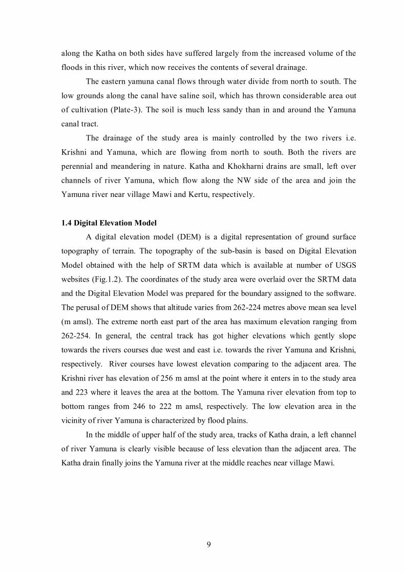
1.4 Digital Elevation Model
A digital elevation model (DEM) is a digital representation of ground surface
topography of terrain. The topography of the sub-basin is based on Digital Elevation
Model obtained with the help of SRTM data which is available at number of USGS
websites (Fig.1.2). The coordinates of the study area were overlaid over the SRTM data
and the Digital Elevation Model was prepared for the boundary assigned to the software.
The perusal of DEM shows that altitude varies from 262-224 metres above mean sea level
(m amsl). The extreme north east part of the area has maximum elevation ranging from
262-254. In general, the central track has got higher elevations which gently slope
towards the rivers courses due west and east i.e. towards the river Yamuna and Krishni,
respectively. River courses have lowest elevation comparing to the adjacent area. The
Krishni river has elevation of 256 m amsl at the point where it enters in to the study area
and 223 where it leaves the area at the bottom. The Yamuna river elevation from top to
bottom ranges from 246 to 222 m amsl, respectively. The low elevation area in the
vicinity of river Yamuna is characterized by flood plains.
In the middle of upper half of the study area, tracks of Katha drain, a left channel
of river Yamuna is clearly visible because of less elevation than the adjacent area. The
Katha drain finally joins the Yamuna river at the middle reaches near village Mawi.
10
Fig.1.2 Digital Elevation Model of Yamuna-Krishni sub basin.
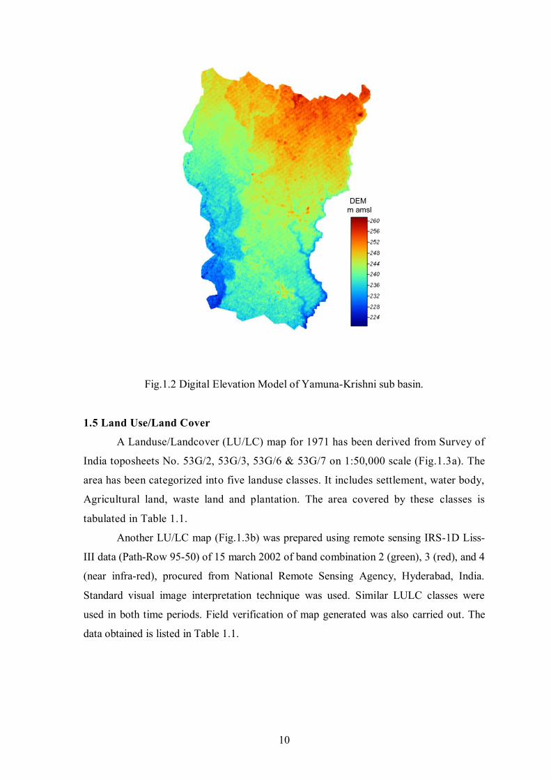
1.5 Land Use/Land Cover
A Landuse/Landcover (LU/LC) map for 1971 has been derived from Survey of
India toposheets No. 53G/2, 53G/3, 53G/6 & 53G/7 on 1:50,000 scale (Fig.1.3a). The
area has been categorized into five landuse classes. It includes settlement, water body,
Agricultural land, waste land and plantation. The area covered by these classes is
tabulated in Table 1.1.
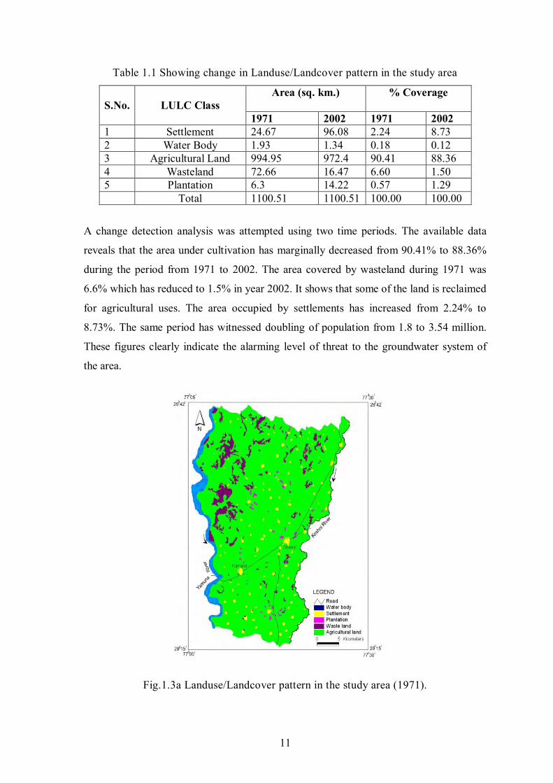
Another LU/LC map (Fig.1.3b) was prepared using remote sensing IRS-1D Liss-
III data (Path-Row 95-50) of 15 march 2002 of band combination 2 (green), 3 (red), and 4
(near infra-red), procured from National Remote Sensing Agency, Hyderabad, India.
Standard visual image interpretation technique was used. Similar LULC classes were
used in both time periods. Field verification of map generated was also carried out. The
data obtained is listed in Table 1.1.
11
Table 1.1 Showing change in Landuse/Landcover pattern in the study area
S.No. LULC Class Area (sq. km.)
% Coverage
1971 2002 1971 2002 1 Settlement 24.67 96.08 2.24 8.73 2 Water Body 1.93 1.34 0.18 0.12 3 Agricultural Land 994.95 972.4 90.41 88.36 4 Wasteland 72.66 16.47 6.60 1.50 5 Plantation 6.3 14.22 0.57 1.29 Total 1100.51 1100.51 100.00 100.00
A change detection analysis was attempted using two time periods. The available data
reveals that the area under cultivation has marginally decreased from 90.41% to 88.36%
during the period from 1971 to 2002. The area covered by wasteland during 1971 was
6.6% which has reduced to 1.5% in year 2002. It shows that some of the land is reclaimed
for agricultural uses. The area occupied by settlements has increased from 2.24% to
8.73%. The same period has witnessed doubling of population from 1.8 to 3.54 million.
These figures clearly indicate the alarming level of threat to the groundwater system of
the area.
Fig.1.3a Landuse/Landcover pattern in the study area (1971).
12
Figure 1.3b Landuse/Landcover pattern in the study area (2002)
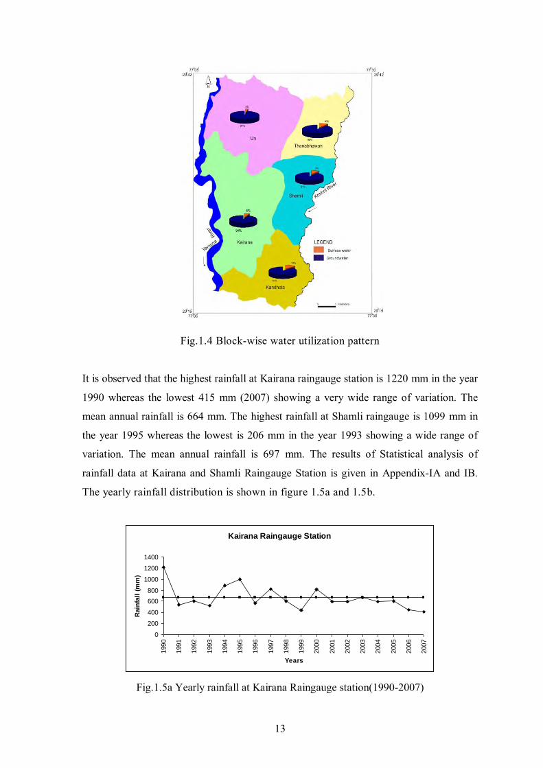
1.6 Water Utilization Pattern
Out of total water resources of the Yamuna-Krishni sub-basin, only 8.1% is
derived from the surface water sources and 91.9% from the groundwater. The Eastern
Yamuna Canal and its distributaries are main source of surface water irrigation.
The block wise water utilization pattern is shown in figure 1.4. A perusal of
figure shows that the blocks traversed by Eastern Yamuna Canal have maximum surface
water utilization which range from 9 to 13% of total water use. In the rest of the blocks
contribution from surface water is, on an average, is less than 5%. These figures clearly
show stress on groundwater regime of the area.
1.7 Rainfall and its Temporal Variability
The available annual rainfall data of Kairana and Shamli raingauge stations for the
period of 1990-2007 and 1990-2007 have been statistically analysed and results are
tabulated in Table 1.2 , respectively.
13
Fig.1.4 Block-wise water utilization pattern
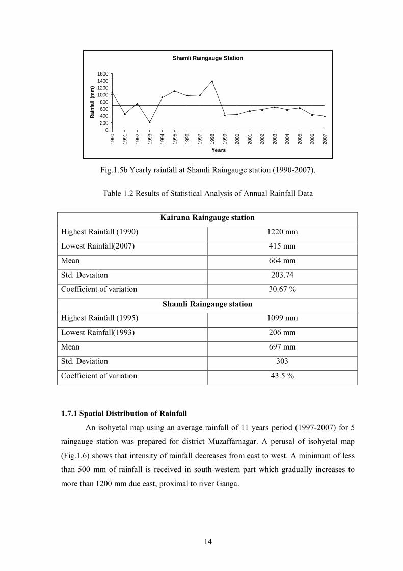
It is observed that the highest rainfall at Kairana raingauge station is 1220 mm in the year
1990 whereas the lowest 415 mm (2007) showing a very wide range of variation. The
mean annual rainfall is 664 mm. The highest rainfall at Shamli raingauge is 1099 mm in
the year 1995 whereas the lowest is 206 mm in the year 1993 showing a wide range of
variation. The mean annual rainfall is 697 mm. The results of Statistical analysis of
rainfall data at Kairana and Shamli Raingauge Station is given in Appendix-IA and IB.
The yearly rainfall distribution is shown in figure 1.5a and 1.5b.
Kairana Raingauge Station
0
200
400
600
800
1000
1200
1400
1990
1991
1992
1993
1994
1995
1996
1997
1998
1999
2000
2001
2002
2003
2004
2005
2006
2007
Years
Rain
fall
(m
m)
Fig.1.5a Yearly rainfall at Kairana Raingauge station(1990-2007)
14
Shamli Raingauge Station
0
200
400
600
800
1000
1200
1400
1600
1990
1991
1992
1993
1994
1995
1996
1997
1998
1999
2000
2001
2002
2003
2004
2005
2006
2007
Years
Rain
fall
(m
m)
Fig.1.5b Yearly rainfall at Shamli Raingauge station (1990-2007).
Table 1.2 Results of Statistical Analysis of Annual Rainfall Data
Kairana Raingauge station
Highest Rainfall (1990) 1220 mm
Lowest Rainfall(2007) 415 mm
Mean 664 mm
Std. Deviation 203.74
Coefficient of variation 30.67 %
Shamli Raingauge station
Highest Rainfall (1995) 1099 mm
Lowest Rainfall(1993) 206 mm
Mean 697 mm
Std. Deviation 303
Coefficient of variation 43.5 %
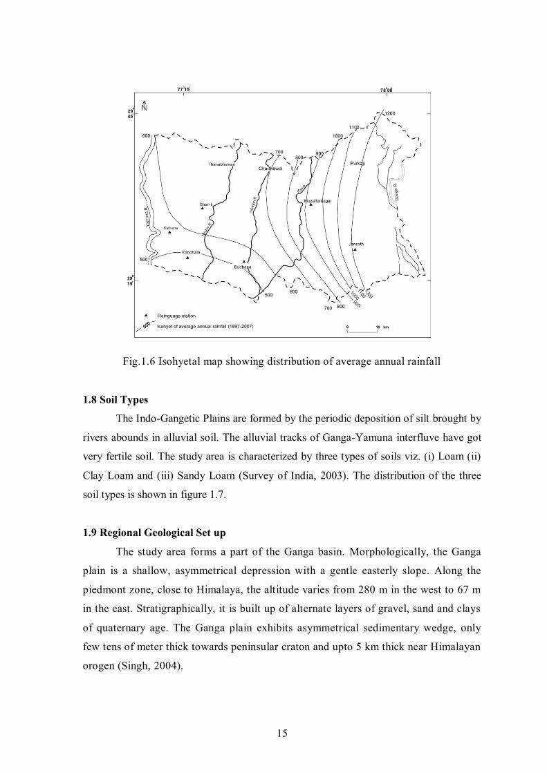
1.7.1 Spatial Distribution of Rainfall
An isohyetal map using an average rainfall of 11 years period (1997-2007) for 5
raingauge station was prepared for district Muzaffarnagar. A perusal of isohyetal map
(Fig.1.6) shows that intensity of rainfall decreases from east to west. A minimum of less
than 500 mm of rainfall is received in south-western part which gradually increases to
more than 1200 mm due east, proximal to river Ganga.
15
Fig.1.6 Isohyetal map showing distribution of average annual rainfall
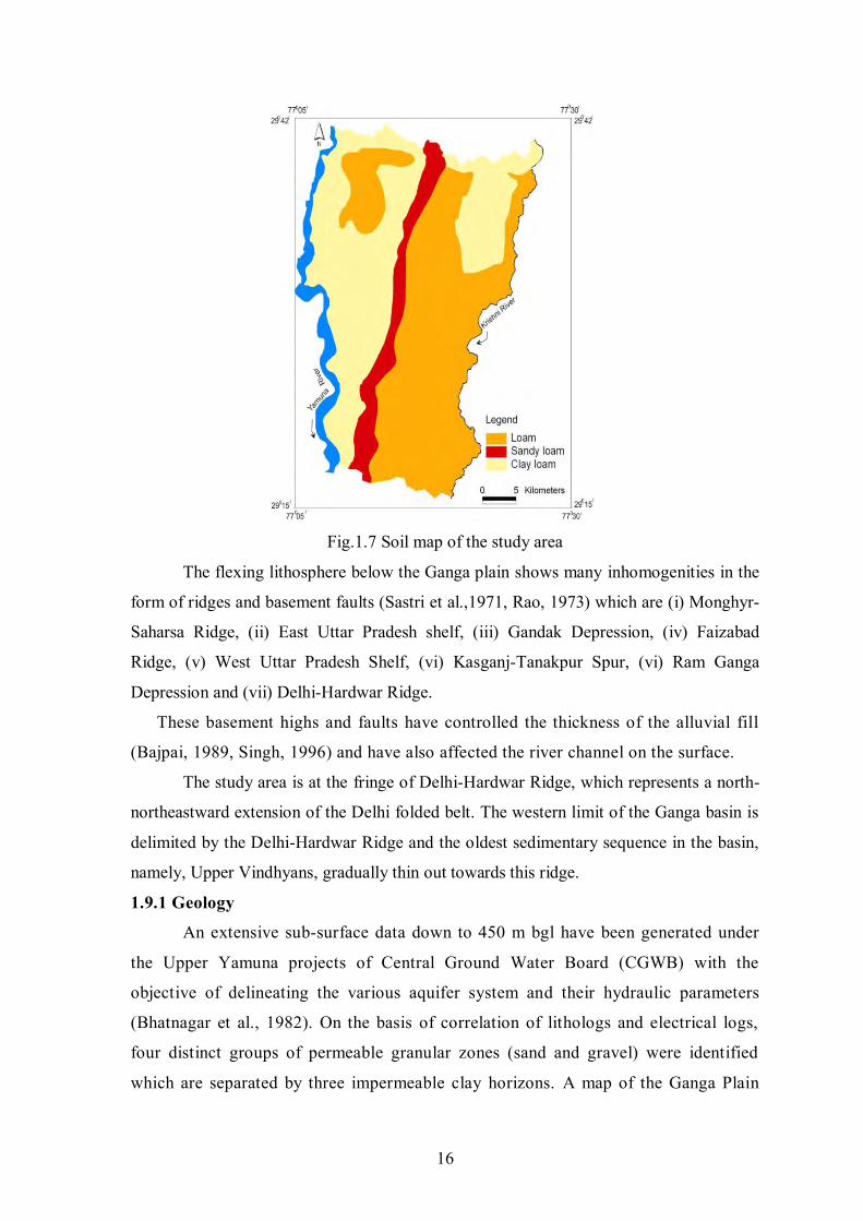
1.8 Soil Types
The Indo-Gangetic Plains are formed by the periodic deposition of silt brought by
rivers abounds in alluvial soil. The alluvial tracks of Ganga-Yamuna interfluve have got
very fertile soil. The study area is characterized by three types of soils viz. (i) Loam (ii)
Clay Loam and (iii) Sandy Loam (Survey of India, 2003). The distribution of the three
soil types is shown in figure 1.7.
1.9 Regional Geological Set up
The study area forms a part of the Ganga basin. Morphologically, the Ganga
plain is a shallow, asymmetrical depression with a gentle easterly slope. Along the
piedmont zone, close to Himalaya, the altitude varies from 280 m in the west to 67 m
in the east. Stratigraphically, it is built up of alternate layers of gravel, sand and clays
of quaternary age. The Ganga plain exhibits asymmetrical sedimentary wedge, only
few tens of meter thick towards peninsular craton and upto 5 km thick near Himalayan
orogen (Singh, 2004).
16
Fig.1.7 Soil map of the study area
The flexing lithosphere below the Ganga plain shows many inhomogenities in the
form of ridges and basement faults (Sastri et al.,1971, Rao, 1973) which are (i) Monghyr-
Saharsa Ridge, (ii) East Uttar Pradesh shelf, (iii) Gandak Depression, (iv) Faizabad
Ridge, (v) West Uttar Pradesh Shelf, (vi) Kasganj-Tanakpur Spur, (vi) Ram Ganga
Depression and (vii) Delhi-Hardwar Ridge.
These basement highs and faults have controlled the thickness of the alluvial fill
(Bajpai, 1989, Singh, 1996) and have also affected the river channel on the surface.
The study area is at the fringe of Delhi-Hardwar Ridge, which represents a north-
northeastward extension of the Delhi folded belt. The western limit of the Ganga basin is
delimited by the Delhi-Hardwar Ridge and the oldest sedimentary sequence in the basin,
namely, Upper Vindhyans, gradually thin out towards this ridge.
1.9.1 Geology
An extensive sub-surface data down to 450 m bgl have been generated under
the Upper Yamuna projects of Central Ground Water Board (CGWB) with the
objective of delineating the various aquifer system and their hydraulic parameters
(Bhatnagar et al., 1982). On the basis of correlation of lithologs and electrical logs,
four distinct groups of permeable granular zones (sand and gravel) were identified
which are separated by three impermeable clay horizons. A map of the Ganga Plain
17
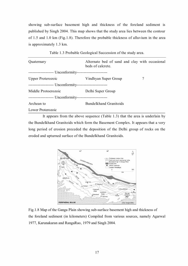
showing sub-surface basement high and thickness of the foreland sediment is
published by Singh 2004. This map shows that the study area lies between the contour
of 1.5 and 1.0 km (Fig.1.8). Therefore the probable thickness of alluvium in the area
is approximately 1.3 km.
Table 1.3 Probable Geological Succession of the study area.
Quaternary Alternate bed of sand and clay with occasional beds of calcrete.
------------------- Unconformity-----------------------
Upper Proterozoic Vindhyan Super Group ? ------------------- Unconformity-----------------------
Middle Protoerozoic Delhi Super Group ------------------- Unconformity-----------------------
Archean to Bundelkhand Granitoids Lower Proterozoic
It appears from the above sequence (Table 1.3) that the area is underlain by
the Bundelkhand Granitoids which form the Basement Complex. It appears that a very
long period of erosion preceded the deposition of the Delhi group of rocks on the
eroded and upturned surface of the Bundelkhand Granitoids.
Fig.1.8 Map of the Ganga Plain showing sub-surface basement high and thickness of
the foreland sediment (in kilometers) Compiled from various sources, namely Agarwal
1977, Karunakaran and RangaRao, 1979 and Singh 2004.
18
2 – HYDROGEOLOGY 2.1 Introduction
The study area is a part of Central Ganga plain. Geologically, the area is
underlain by alluvial deposits of Quaternary age, approximately 1000 m in thickness.
The alluvium is underlain by Middle Proterozoic Delhi quartzites. The quartzites, in
turn, are underlain by Bundelkhand Granitoid (3000 Ma). The alluvium in Krishni-
Yamuna interfluve region consists of alternate beds of sand and clay with occasional
interbeds of calc-concretion (Kankar). The methodology of aquifer characterization
are discussed in preceding sections.
2.2 Aquifer geometry
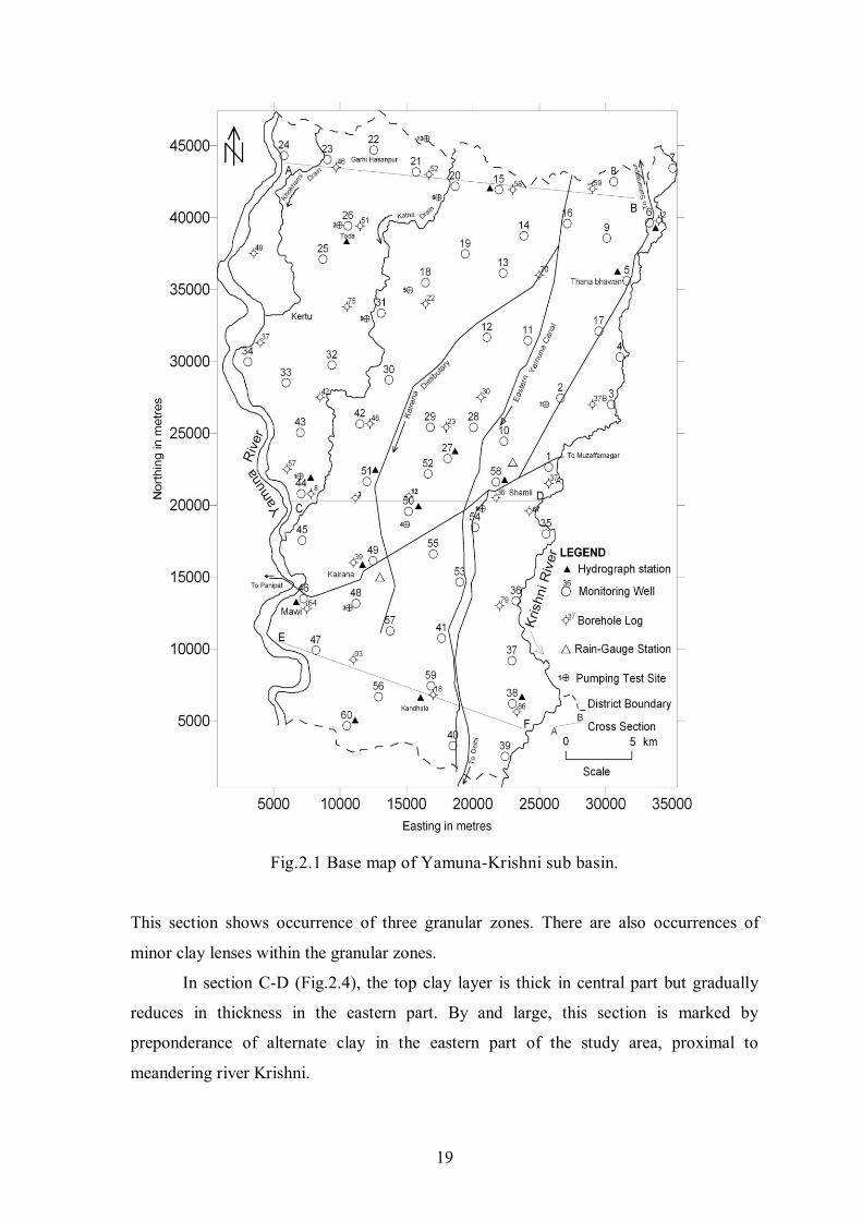
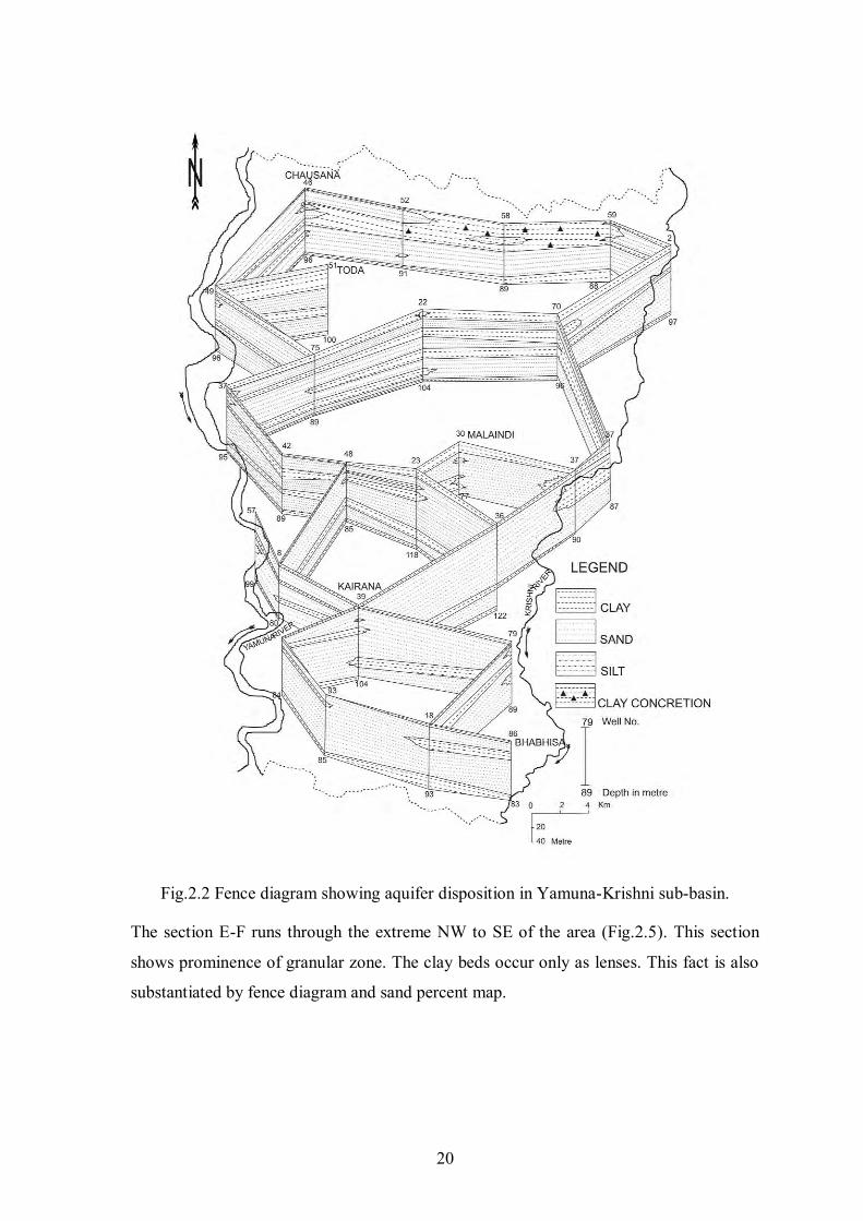
A Fence diagram based on lithological logs of borehole (Fig.2.1) drilled by State
Tubewell Department has been prepared (Appendix III). The fence diagram (Fig.2.2)
reveals the vertical and lateral disposition of aquifers, aquiclude and aquitard in the study
area down to depth of 122 m bgl. Nature of alluvial sediments is generally complex and
there is quick alteration of pervious and impervious layer. The top clay layer is persistent
through out the area varying in thickness from 3 to 20 m bgl. The top clay bed is
underlain by granular zone, which extends downward to different depths varying up to
122 m bgl. The granular material is composed of fine, medium to coarse sand. The
granular zone is subdivided at places into two to three sub-groups by occurrence of sub-
regional clay beds, local clay lenses are also common through out the area. By and large
the aquifer down to 122 m appears to merge with each other and behaves as single bodied
aquifer.
Granular zone composed of medium to coarse sand and gravel form about 80-90
% of total formation encountered, particularly in southeastern and southern part of the
basin. This area being a down faulted area due to NE-SW Muzaffarnagar fault possibly
became a dominant recipient of sand than the area north of the fault. Muzaffarnagar fault
is an active transverse E-W running fault, with through to the south side and passing
through the Muzaffarnagar city (Bhosle et al., 2007).
In addition to fence diagram three hydrogeological cross section A-B, C-D and E-
F (Fig.2.1) are distributed across the entire area in which two sections run from west to
east and the section E-F from north west to south east.
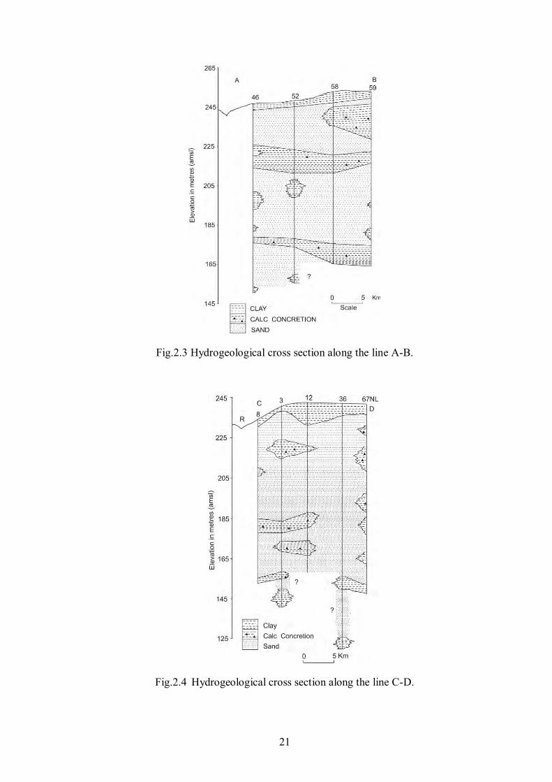
The section A-B (Fig.2.3) represent extreme north of the area. A perusal of the
section A-B reveals the clay bed occurs in repeated alternation with in granular zone.
19
Fig.2.1 Base map of Yamuna-Krishni sub basin.
This section shows occurrence of three granular zones. There are also occurrences of
minor clay lenses within the granular zones.
In section C-D (Fig.2.4), the top clay layer is thick in central part but gradually
reduces in thickness in the eastern part. By and large, this section is marked by
preponderance of alternate clay in the eastern part of the study area, proximal to
meandering river Krishni.
20
Fig.2.2 Fence diagram showing aquifer disposition in Yamuna-Krishni sub-basin.
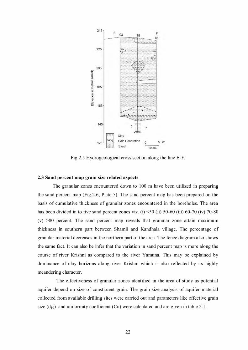
The section E-F runs through the extreme NW to SE of the area (Fig.2.5). This section
shows prominence of granular zone. The clay beds occur only as lenses. This fact is also
substantiated by fence diagram and sand percent map.
21
Fig.2.3 Hydrogeological cross section along the line A-B.
Fig.2.4 Hydrogeological cross section along the line C-D.
22
Fig.2.5 Hydrogeological cross section along the line E-F.
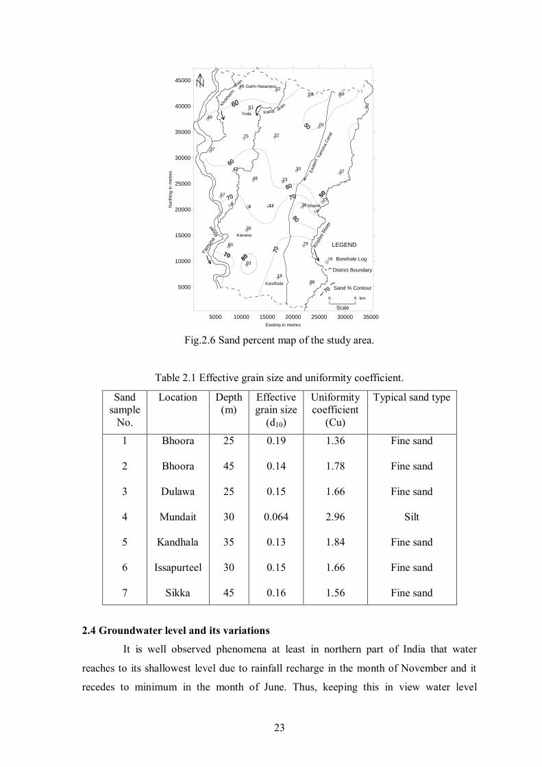
2.3 Sand percent map grain size related aspects
The granular zones encountered down to 100 m have been utilized in preparing
the sand percent map (Fig.2.6, Plate 5). The sand percent map has been prepared on the
basis of cumulative thickness of granular zones encountered in the boreholes. The area
has been divided in to five sand percent zones viz. (i) <50 (ii) 50-60 (iii) 60-70 (iv) 70-80
(v) >80 percent. The sand percent map reveals that granular zone attain maximum
thickness in southern part between Shamli and Kandhala village. The percentage of
granular material decreases in the northern part of the area. The fence diagram also shows
the same fact. It can also be infer that the variation in sand percent map is more along the
course of river Krishni as compared to the river Yamuna. This may be explained by
dominance of clay horizons along river Krishni which is also reflected by its highly
meandering character.
The effectiveness of granular zones identified in the area of study as potential
aquifer depend on size of constituent grain. The grain size analysis of aquifer material
collected from available drilling sites were carried out and parameters like effective grain
size (d10) and uniformity coefficient (Cu) were calculated and are given in table 2.1.
23
5000 10000 15000 20000 25000 30000 35000
Easting in metres
5000
10000
15000
20000
25000
30000
35000
40000
45000
No
rthin
g in
metr
es
37
37
2
58
22
5246
51
30
23
79
86
48
8
80
93
39
36
18
59
70
57
42
49
37
75
Borehole Log
LEGEND
Kairana
Shamli
Toda
Kandhala
District Boundary
Garhi Hasanpur
East
ern
Yam
una C
anal
Katha drainK
hokh
arni
drain
0 5 km
Scale
3 1267
1880
70
50
Yam
una
Riv
er
Krish
ni R
iver
Sand % Contour
Fig.2.6 Sand percent map of the study area.
Table 2.1 Effective grain size and uniformity coefficient.
Sand sample
No.
Location Depth (m)
Effective grain size
(d10)
Uniformity coefficient
(Cu)
Typical sand type
1
2
3
4
5
6
7
Bhoora
Bhoora
Dulawa
Mundait
Kandhala
Issapurteel
Sikka
25
45
25
30
35
30
45
0.19
0.14
0.15
0.064
0.13
0.15
0.16
1.36
1.78
1.66
2.96
1.84
1.66
1.56
Fine sand
Fine sand
Fine sand
Silt
Fine sand
Fine sand
Fine sand
2.4 Groundwater level and its variations
It is well observed phenomena at least in northern part of India that water
reaches to its shallowest level due to rainfall recharge in the month of November and it
recedes to minimum in the month of June. Thus, keeping this in view water level
24
monitoring was initially planed during these periods. Water level data was collected from
observation wells with the help of steel tape. Due care was given for accurately
measuring the water level data. Groundwater level in an unconfined aquifer is much
sensitive to fluctuation. Thus error may introduce because of pumping influence in near
by area, river stage and also because of groundwater movements. The data collected
(Plate 4a, b & c) were used in interpretation of depth, slope, movement and fluctuation of
water level.
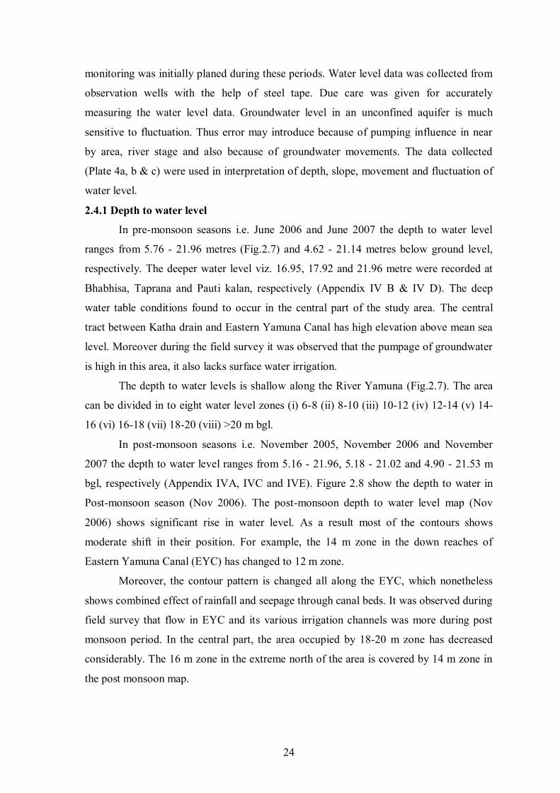
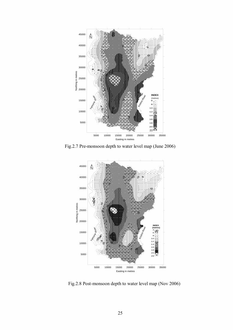
2.4.1 Depth to water level
In pre-monsoon seasons i.e. June 2006 and June 2007 the depth to water level
ranges from 5.76 - 21.96 metres (Fig.2.7) and 4.62 - 21.14 metres below ground level,
respectively. The deeper water level viz. 16.95, 17.92 and 21.96 metre were recorded at
Bhabhisa, Taprana and Pauti kalan, respectively (Appendix IV B & IV D). The deep
water table conditions found to occur in the central part of the study area. The central
tract between Katha drain and Eastern Yamuna Canal has high elevation above mean sea
level. Moreover during the field survey it was observed that the pumpage of groundwater
is high in this area, it also lacks surface water irrigation.
The depth to water levels is shallow along the River Yamuna (Fig.2.7). The area
can be divided in to eight water level zones (i) 6-8 (ii) 8-10 (iii) 10-12 (iv) 12-14 (v) 14-
16 (vi) 16-18 (vii) 18-20 (viii) >20 m bgl.
In post-monsoon seasons i.e. November 2005, November 2006 and November
2007 the depth to water level ranges from 5.16 - 21.96, 5.18 - 21.02 and 4.90 - 21.53 m
bgl, respectively (Appendix IVA, IVC and IVE). Figure 2.8 show the depth to water in
Post-monsoon season (Nov 2006). The post-monsoon depth to water level map (Nov
2006) shows significant rise in water level. As a result most of the contours shows
moderate shift in their position. For example, the 14 m zone in the down reaches of
Eastern Yamuna Canal (EYC) has changed to 12 m zone.
Moreover, the contour pattern is changed all along the EYC, which nonetheless
shows combined effect of rainfall and seepage through canal beds. It was observed during
field survey that flow in EYC and its various irrigation channels was more during post
monsoon period. In the central part, the area occupied by 18-20 m zone has decreased
considerably. The 16 m zone in the extreme north of the area is covered by 14 m zone in
the post monsoon map.
25
5000 10000 15000 20000 25000 30000 35000
Easting in metres
5000
10000
15000
20000
25000
30000
35000
40000
45000
No
rth
ing
in
me
tre
s
Yam
una
Riv
er
Krish
ni R
iver
6
8
10
12
14
16
18
20
INDEX
(metres)86
22
Fig.2.7 Pre-monsoon depth to water level map (June 2006)
5000 10000 15000 20000 25000 30000 35000
Easting in metres
5000
10000
15000
20000
25000
30000
35000
40000
45000
Nort
hin
g in m
etr
es
Yam
una
Riv
er
Krish
ni R
iver
4
6
8
10
12
14
16
18
20
22
INDEX(metres)
Fig.2.8 Post-monsoon depth to water level map (Nov 2006)
26
The change in contour pattern in command and non-command area is, in all likelihood,
infer that the increase in groundwater storage is because of rainfall recharge, irrigation
return and through canal seepage as well.
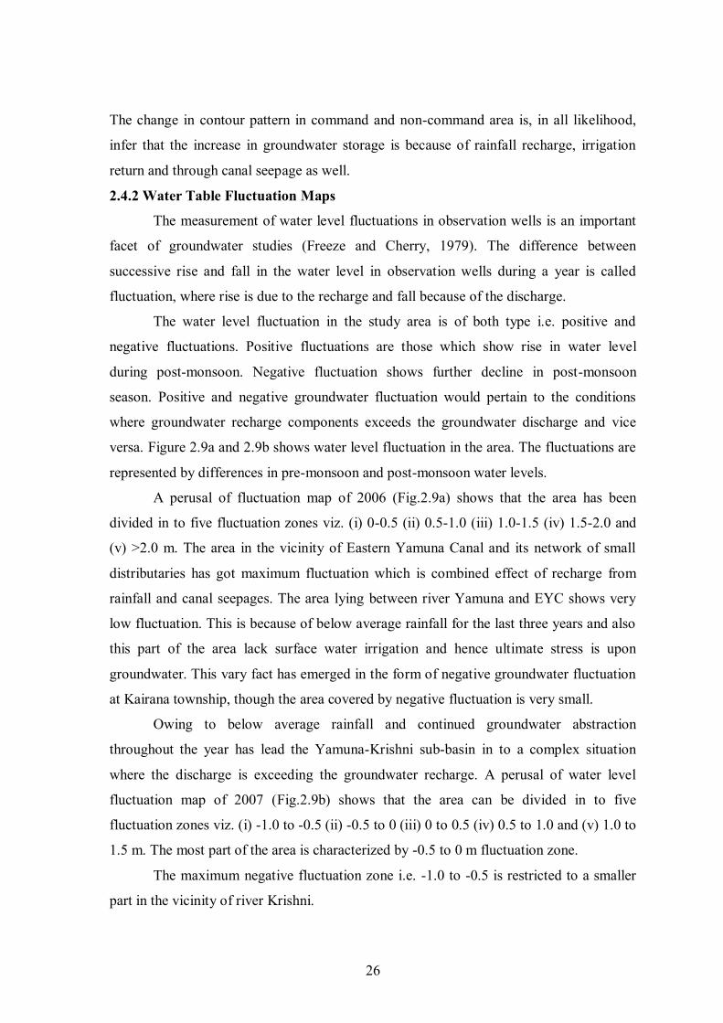
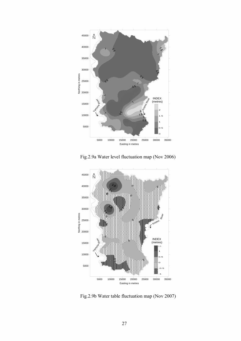
2.4.2 Water Table Fluctuation Maps
The measurement of water level fluctuations in observation wells is an important
facet of groundwater studies (Freeze and Cherry, 1979). The difference between
successive rise and fall in the water level in observation wells during a year is called
fluctuation, where rise is due to the recharge and fall because of the discharge.
The water level fluctuation in the study area is of both type i.e. positive and
negative fluctuations. Positive fluctuations are those which show rise in water level
during post-monsoon. Negative fluctuation shows further decline in post-monsoon
season. Positive and negative groundwater fluctuation would pertain to the conditions
where groundwater recharge components exceeds the groundwater discharge and vice
versa. Figure 2.9a and 2.9b shows water level fluctuation in the area. The fluctuations are
represented by differences in pre-monsoon and post-monsoon water levels.
A perusal of fluctuation map of 2006 (Fig.2.9a) shows that the area has been
divided in to five fluctuation zones viz. (i) 0-0.5 (ii) 0.5-1.0 (iii) 1.0-1.5 (iv) 1.5-2.0 and
(v) >2.0 m. The area in the vicinity of Eastern Yamuna Canal and its network of small
distributaries has got maximum fluctuation which is combined effect of recharge from
rainfall and canal seepages. The area lying between river Yamuna and EYC shows very
low fluctuation. This is because of below average rainfall for the last three years and also
this part of the area lack surface water irrigation and hence ultimate stress is upon
groundwater. This vary fact has emerged in the form of negative groundwater fluctuation
at Kairana township, though the area covered by negative fluctuation is very small.
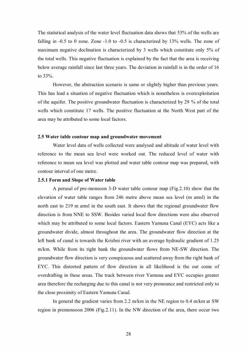
Owing to below average rainfall and continued groundwater abstraction
throughout the year has lead the Yamuna-Krishni sub-basin in to a complex situation
where the discharge is exceeding the groundwater recharge. A perusal of water level
fluctuation map of 2007 (Fig.2.9b) shows that the area can be divided in to five
fluctuation zones viz. (i) -1.0 to -0.5 (ii) -0.5 to 0 (iii) 0 to 0.5 (iv) 0.5 to 1.0 and (v) 1.0 to
1.5 m. The most part of the area is characterized by -0.5 to 0 m fluctuation zone.
The maximum negative fluctuation zone i.e. -1.0 to -0.5 is restricted to a smaller
part in the vicinity of river Krishni.
27
5000 10000 15000 20000 25000 30000 35000
Easting in metres
5000
10000
15000
20000
25000
30000
35000
40000
45000
Nort
hin
g in m
etr
es
0
0.5
1
1.5
2
Yam
una
Riv
er
Krish
ni R
iver INDEX
(metres)
Fig.2.9a Water level fluctuation map (Nov 2006)
5000 10000 15000 20000 25000 30000 35000
Easting in metres
5000
10000
15000
20000
25000
30000
35000
40000
45000
No
rth
ng
in m
etr
es
Krishni
Riv
er
Yam
una
Riv
er
1.5
1.0
-1
-0.5
0
0.5
1
1.5
INDEX(metres)
Fig.2.9b Water table fluctuation map (Nov 2007)
28
The statistical analysis of the water level fluctuation data shows that 53% of the wells are
falling in -0.5 to 0 zone. Zone -1.0 to -0.5 is characterized by 13% wells. The zone of
maximum negative declination is characterized by 3 wells which constitute only 5% of
the total wells. This negative fluctuation is explained by the fact that the area is receiving
below average rainfall since last three years. The deviation in rainfall is in the order of 16
to 33%.
However, the abstraction scenario is same or slightly higher than previous years.
This has lead a situation of negative fluctuation which is nonetheless is overexploitation
of the aquifer. The positive groundwater fluctuation is characterized by 29 % of the total
wells which constitute 17 wells. The positive fluctuation at the North West part of the
area may be attributed to some local factors.
2.5 Water table contour map and groundwater movement
Water level data of wells collected were analysed and altitude of water level with
reference to the mean sea level were worked out. The reduced level of water with
reference to mean sea level was plotted and water table contour map was prepared, with
contour interval of one metre.
2.5.1 Form and Slope of Water table
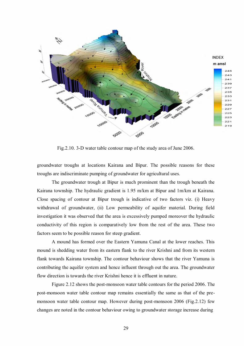
A perusal of pre-monsoon 3-D water table contour map (Fig.2.10) show that the
elevation of water table ranges from 246 metre above mean sea level (m amsl) in the
north east to 219 m amsl in the south east. It shows that the regional groundwater flow
direction is from NNE to SSW. Besides varied local flow directions were also observed
which may be attributed to some local factors. Eastern Yamuna Canal (EYC) acts like a
groundwater divide, almost throughout the area. The groundwater flow direction at the
left bank of canal is towards the Krishni river with an average hydraulic gradient of 1.25
m/km. While from its right bank the groundwater flows from NE-SW direction. The
groundwater flow direction is very conspicuous and scattered away from the right bank of
EYC. This distorted pattern of flow direction in all likelihood is the out come of
overdrafting in these areas. The track between river Yamuna and EYC occupies greater
area therefore the recharging due to this canal is not very pronounce and restricted only to
the close proximity of Eastern Yamuna Canal.
In general the gradient varies from 2.2 m/km in the NE region to 0.4 m/km at SW
region in premonsoon 2006 (Fig.2.11). In the NW direction of the area, there occur two
29
Fig.2.10. 3-D water table contour map of the study area of June 2006.
groundwater troughs at locations Kairana and Bipur. The possible reasons for these
troughs are indiscriminate pumping of groundwater for agricultural uses.
The groundwater trough at Bipur is much prominent than the trough beneath the
Kairana township. The hydraulic gradient is 1.95 m/km at Bipur and 1m/km at Kairana.
Close spacing of contour at Bipur trough is indicative of two factors viz. (i) Heavy
withdrawal of groundwater, (ii) Low permeability of aquifer material. During field
investigation it was observed that the area is excessively pumped moreover the hydraulic
conductivity of this region is comparatively low from the rest of the area. These two
factors seem to be possible reason for steep gradient.
A mound has formed over the Eastern Yamuna Canal at the lower reaches. This
mound is shedding water from its eastern flank to the river Krishni and from its western
flank towards Kairana township. The contour behaviour shows that the river Yamuna is
contributing the aquifer system and hence influent through out the area. The groundwater
flow direction is towards the river Krishni hence it is effluent in nature.
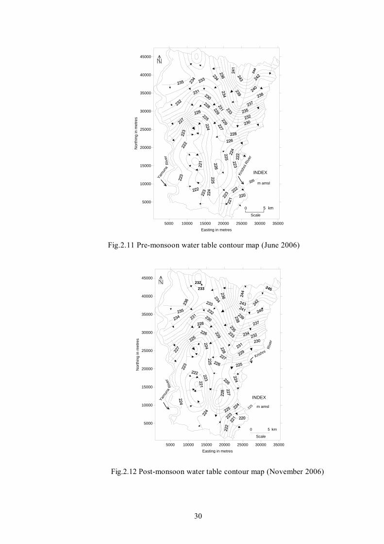
Figure 2.12 shows the post-monsoon water table contours for the period 2006. The
post-monsoon water table contour map remains essentially the same as that of the pre-
monsoon water table contour map. However during post-monsoon 2006 (Fig.2.12) few
changes are noted in the contour behaviour owing to groundwater storage increase during
30
5000 10000 15000 20000 25000 30000 35000
Easting in metres
5000
10000
15000
20000
25000
30000
35000
40000
45000
Nort
hin
g in m
etr
es
Yam
una
Riv
er
Krish
ni R
iver
0 5 km
m amsl
INDEX
244
Scale
Fig.2.11 Pre-monsoon water table contour map (June 2006)
5000 10000 15000 20000 25000 30000 35000
Easting in metres
5000
10000
15000
20000
25000
30000
35000
40000
45000
Nort
hin
g in m
etr
es
Krishni
Riv
er
Yam
una
Riv
er
0 5 km
225 m amsl
INDEX
233
232245
Scale
Fig.2.12 Post-monsoon water table contour map (November 2006)
31
post-monsoon period which are discussed below few changes are brought about in shape
of the contours and are somewhat displaced by higher contour values. The groundwater
troughs at the location Pauti and Kairana is present in both the season for year 2006 and
hence seems to be permanent in nature.
2.6 Long term behaviour of water levels
2.6.1 Biannually water level monitoring
Historical water level data of fourteen permanent hydrograph stations were
collected from Central Ground Water Board (CGWB) and State Groundwater Department
(UPSGWD). The data were utilized to prepare hydrograph with a view to study their
behaviour with respect to time and space and their dependence on natural phenomenon.
The water levels in unconfined aquifers are affected by direct recharge from precipitation,
evapotranspiration, withdrawals from the wells, discharge to streams, and sometimes
changes in atmospheric pressure. From the above discussion it has been inferred that the
water level has a rising and declining trend with respect to time and a function which
causes such rises in water levels i.e. availability of rainfall.
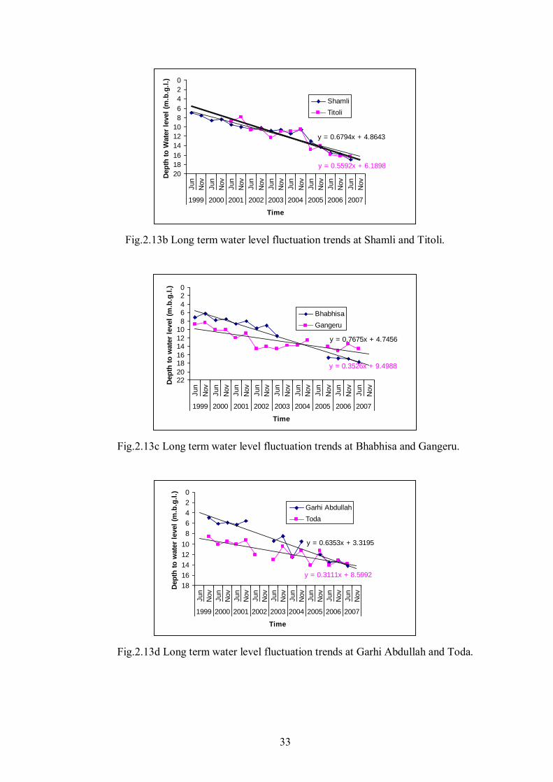
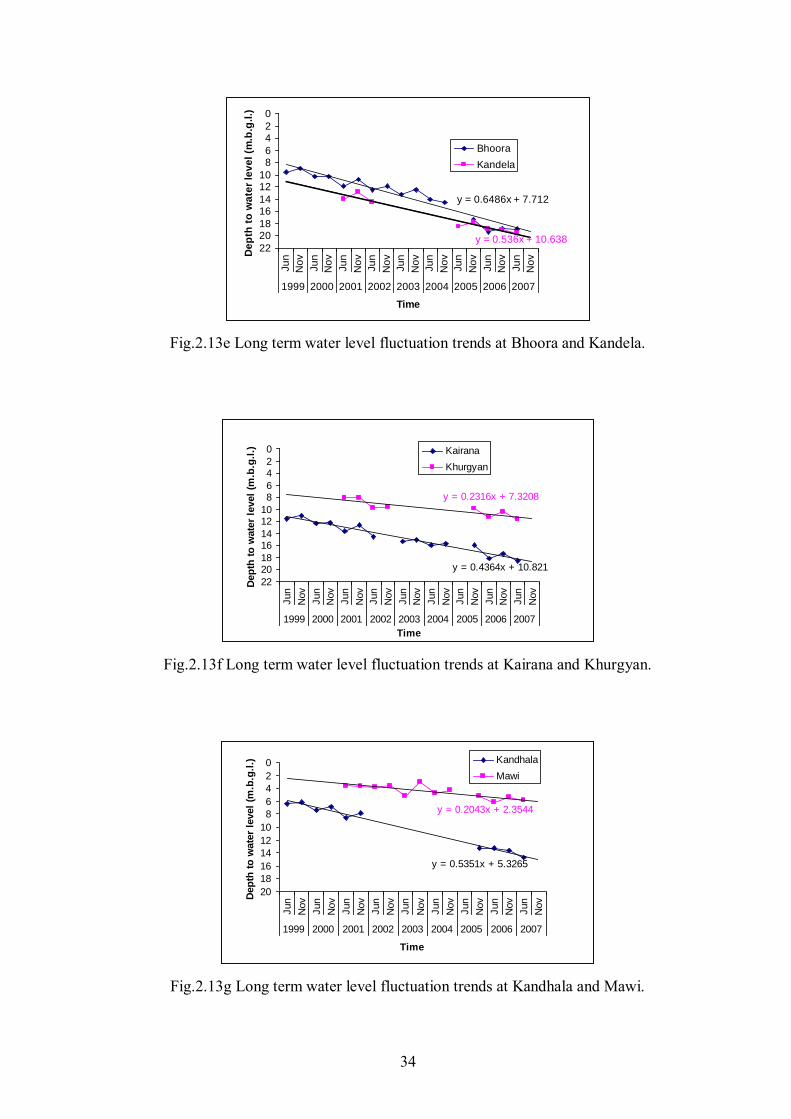
Perusals of hydrographs (Fig.2.13a, b, c, d, e, f, & g) indicate that the water
level variation is cyclic and sinusoidal as a function of time and space. For a year, the
water level is deepest during the month of June and shallowest during the month of
November. It is observed that the water level starts rising by last week of June and attains
shallowest level in November. In overdeveloped areas a downward trend of water
levels may continue for many years because of continual increases in pumpage or
withdrawals in excess of recharge, or both.
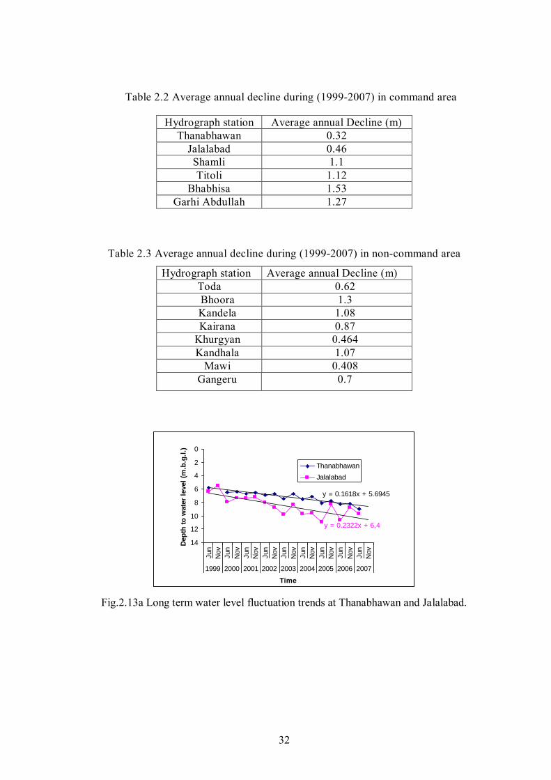
It is seen from the hydrographs that there is progressive decline in the water
level trend with in the study area, especially for last three-four years, the decline trend
seems pronounced and persistent. A trend line was fitted on the graphs using t-statistic for
testing significance of observed regression coefficient, the values of r-square and r for the
given data set shows 95% level of confidence. The average annual decline in command
and non-command area is given in Table 2.2 & 2.3. The hydrograph data for non-
command and command area is given in Appendix V A and V B, respectively.
32
Table 2.2 Average annual decline during (1999-2007) in command area
Hydrograph station Average annual Decline (m) Thanabhawan 0.32
Jalalabad 0.46 Shamli 1.1 Titoli 1.12
Bhabhisa 1.53 Garhi Abdullah 1.27
Table 2.3 Average annual decline during (1999-2007) in non-command area
Hydrograph station Average annual Decline (m) Toda 0.62 Bhoora 1.3 Kandela 1.08 Kairana 0.87
Khurgyan 0.464 Kandhala 1.07
Mawi 0.408 Gangeru 0.7
y = 0.1618x + 5.6945
y = 0.2322x + 6.4
0
2
4
6
8
10
12
14
Jun
Nov
Jun
Nov
Jun
Nov
Jun
Nov
Jun
Nov
Jun
Nov
Jun
Nov
Jun
Nov
Jun
Nov
1999 2000 2001 2002 2003 2004 2005 2006 2007
Time
Dep
th t
o w
ate
r le
vel
(m.b
.g.l
.)
Thanabhawan
Jalalabad
Fig.2.13a Long term water level fluctuation trends at Thanabhawan and Jalalabad.
33
y = 0.6794x + 4.8643
y = 0.5592x + 6.1898
0
2
4
6
8
10
12
14
16
18
20
Jun
Nov
Jun
Nov
Jun
Nov
Jun
Nov
Jun
Nov
Jun
Nov
Jun
Nov
Jun
Nov
Jun
Nov
1999 2000 2001 2002 2003 2004 2005 2006 2007
Time
Dep
th t
o W
ate
r le
vel
(m.b
.g.l
.)
Shamli
Titoli
Fig.2.13b Long term water level fluctuation trends at Shamli and Titoli.
y = 0.7675x + 4.7456
y = 0.3526x + 9.4988
02
46
810
1214
1618
2022
Jun
Nov
Jun
Nov
Jun
Nov
Jun
Nov
Jun
Nov
Jun
Nov
Jun
Nov
Jun
Nov
Jun
Nov
1999 2000 2001 2002 2003 2004 2005 2006 2007
Time
Dep
th t
o w
ate
r le
vel
(m.b
.g.l
.)
Bhabhisa
Gangeru
Fig.2.13c Long term water level fluctuation trends at Bhabhisa and Gangeru.
y = 0.6353x + 3.3195
y = 0.3111x + 8.5992
0
2
4
6
8
10
12
14
16
18
Jun
Nov
Jun
Nov
Jun
Nov
Jun
Nov
Jun
Nov
Jun
Nov
Jun
Nov
Jun
Nov
Jun
Nov
1999 2000 2001 2002 2003 2004 2005 2006 2007
Time
Dep
th t
o w
ate
r le
vel
(m.b
.g.l
.)
Garhi Abdullah
Toda
Fig.2.13d Long term water level fluctuation trends at Garhi Abdullah and Toda.
34
y = 0.6486x + 7.712
y = 0.536x + 10.638
0
24
68
1012
1416
1820
22
Ju
n
No
v
Ju
n
No
v
Ju
n
No
v
Ju
n
No
v
Ju
n
No
v
Ju
n
No
v
Ju
n
No
v
Ju
n
No
v
Ju
n
No
v
1999 2000 2001 2002 2003 2004 2005 2006 2007
Time
De
pth
to
wa
ter
lev
el
(m.b
.g.l
.)
Bhoora
Kandela
Fig.2.13e Long term water level fluctuation trends at Bhoora and Kandela.
y = 0.2316x + 7.3208
y = 0.4364x + 10.821
0
24
68
1012
1416
1820
22
Jun
Nov
Jun
Nov
Jun
Nov
Jun
Nov
Jun
Nov
Jun
Nov
Jun
Nov
Jun
Nov
Jun
Nov
1999 2000 2001 2002 2003 2004 2005 2006 2007
Time
Dep
th t
o w
ate
r le
vel
(m.b
.g.l
.) Kairana
Khurgyan
Fig.2.13f Long term water level fluctuation trends at Kairana and Khurgyan.
y = 0.2043x + 2.3544
y = 0.5351x + 5.3265
0
2
4
6
8
10
12
14
16
18
20
Jun
Nov
Jun
Nov
Jun
Nov
Jun
Nov
Jun
Nov
Jun
Nov
Jun
Nov
Jun
Nov
Jun
Nov
1999 2000 2001 2002 2003 2004 2005 2006 2007
Time
Dep
th t
o w
ate
r le
vel
(m.b
.g.l
.) Kandhala
Mawi
Fig.2.13g Long term water level fluctuation trends at Kandhala and Mawi.
35
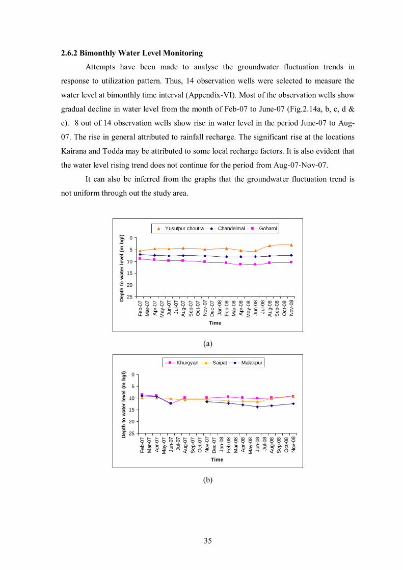
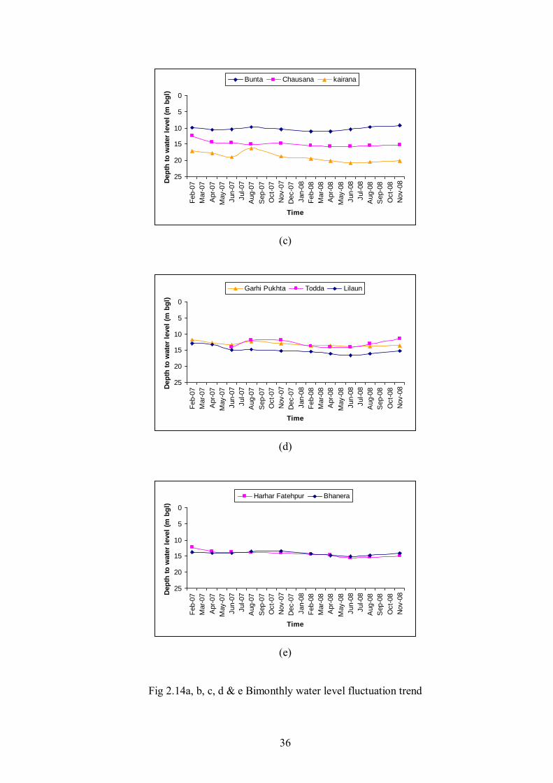
2.6.2 Bimonthly Water Level Monitoring
Attempts have been made to analyse the groundwater fluctuation trends in
response to utilization pattern. Thus, 14 observation wells were selected to measure the
water level at bimonthly time interval (Appendix-VI). Most of the observation wells show
gradual decline in water level from the month of Feb-07 to June-07 (Fig.2.14a, b, c, d &
e). 8 out of 14 observation wells show rise in water level in the period June-07 to Aug-
07. The rise in general attributed to rainfall recharge. The significant rise at the locations
Kairana and Todda may be attributed to some local recharge factors. It is also evident that
the water level rising trend does not continue for the period from Aug-07-Nov-07.
It can also be inferred from the graphs that the groundwater fluctuation trend is
not uniform through out the study area.
0
5
10
15
20
25
Feb-0
7
Mar-
07
Apr-
07
May-0
7
Jun-0
7
Jul-07
Aug-0
7
Sep-0
7
Oct-
07
Nov-0
7
Dec-0
7
Jan-0
8
Feb-0
8
Mar-
08
Apr-
08
May-0
8
Jun-0
8
Jul-08
Aug-0
8
Sep-0
8
Oct-
08
Nov-0
8
Time
Dep
th t
o w
ate
r le
vel
(m b
gl)
Yusufpur choutra Chandelmal Goharni
(a)
0
5
10
15
20
25
Feb-0
7
Mar-
07
Apr-
07
May-0
7
Jun-0
7
Jul-07
Aug-0
7
Sep-0
7
Oct-
07
Nov-0
7
Dec-0
7
Jan-0
8
Feb-0
8
Mar-
08
Apr-
08
May-0
8
Jun-0
8
Jul-08
Aug-0
8
Sep-0
8
Oct-
08
Nov-0
8
Time
Dep
th t
o w
ate
r le
vel
(m b
gl)
Khurgyan Saipat Malakpur
(b)
36
0
5
10
15
20
25
Feb-0
7
Mar-
07
Apr-
07
May-0
7
Jun-0
7
Jul-07
Aug-0
7
Sep-0
7
Oct-
07
Nov-0
7
Dec-0
7
Jan-0
8
Feb-0
8
Mar-
08
Apr-
08
May-0
8
Jun-0
8
Jul-08
Aug-0
8
Sep-0
8
Oct-
08
Nov-0
8
Time
Dep
th t
o w
ate
r le
vel
(m b
gl)
Bunta Chausana kairana
(c)
0
5
10
15
20
25
Feb-0
7
Mar-
07
Apr-
07
May-0
7
Jun-0
7
Jul-07
Aug-0
7
Sep-0
7
Oct-
07
Nov-0
7
Dec-0
7
Jan-0
8
Feb-0
8
Mar-
08
Apr-
08
May-0
8
Jun-0
8
Jul-08
Aug-0
8
Sep-0
8
Oct-
08
Nov-0
8
Time
Dep
th t
o w
ate
r le
vel
(m b
gl)
Garhi Pukhta Todda Lilaun
(d)
0
5
10
15
20
25
Feb-0
7
Mar-
07
Apr-
07
May-0
7
Jun-0
7
Jul-07
Aug-0
7
Sep-0
7
Oct-
07
Nov-0
7
Dec-0
7
Jan-0
8
Feb-0
8
Mar-
08
Apr-
08
May-0
8
Jun-0
8
Jul-08
Aug-0
8
Sep-0
8
Oct-
08
Nov-0
8
Time
Dep
th t
o w
ate
r le
vel
(m b
gl)
Harhar Fatehpur Bhanera
(e)
Fig 2.14a, b, c, d & e Bimonthly water level fluctuation trend
37
The Sharp decline (>2 m) was observed at Malakpur and Khurgyan, both location
are fairly apart, indicate that the local recharge-discharge factors are influential in
determining fluctuation trend.
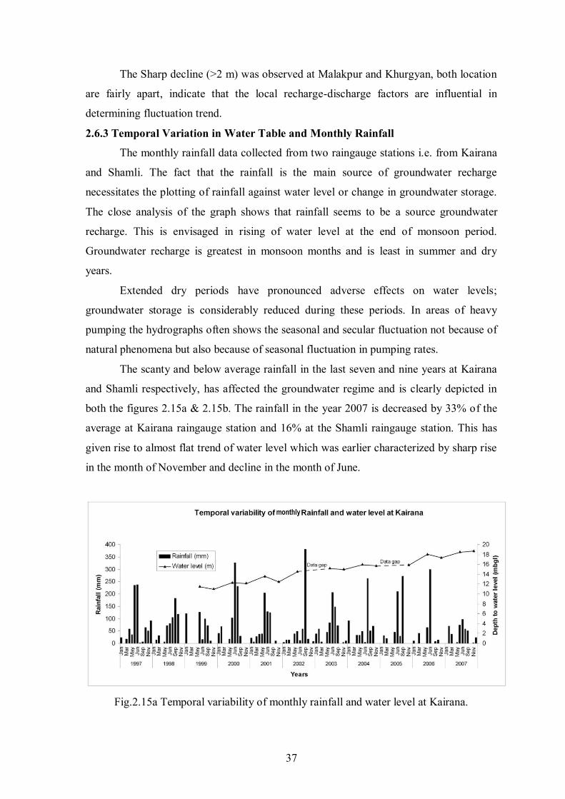
2.6.3 Temporal Variation in Water Table and Monthly Rainfall
The monthly rainfall data collected from two raingauge stations i.e. from Kairana
and Shamli. The fact that the rainfall is the main source of groundwater recharge
necessitates the plotting of rainfall against water level or change in groundwater storage.
The close analysis of the graph shows that rainfall seems to be a source groundwater
recharge. This is envisaged in rising of water level at the end of monsoon period.
Groundwater recharge is greatest in monsoon months and is least in summer and dry
years.
Extended dry periods have pronounced adverse effects on water levels;
groundwater storage is considerably reduced during these periods. In areas of heavy
pumping the hydrographs often shows the seasonal and secular fluctuation not because of
natural phenomena but also because of seasonal fluctuation in pumping rates.
The scanty and below average rainfall in the last seven and nine years at Kairana
and Shamli respectively, has affected the groundwater regime and is clearly depicted in
both the figures 2.15a & 2.15b. The rainfall in the year 2007 is decreased by 33% of the
average at Kairana raingauge station and 16% at the Shamli raingauge station. This has
given rise to almost flat trend of water level which was earlier characterized by sharp rise
in the month of November and decline in the month of June.
Fig.2.15a Temporal variability of monthly rainfall and water level at Kairana.
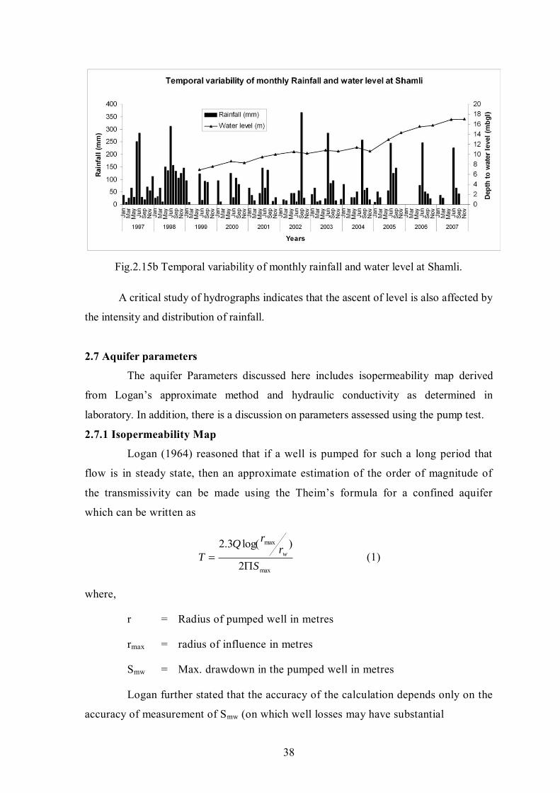
38
Fig.2.15b Temporal variability of monthly rainfall and water level at Shamli.
A critical study of hydrographs indicates that the ascent of level is also affected by
the intensity and distribution of rainfall.
2.7 Aquifer parameters
The aquifer Parameters discussed here includes isopermeability map derived
from Logan’s approximate method and hydraulic conductivity as determined in
laboratory. In addition, there is a discussion on parameters assessed using the pump test.
2.7.1 Isopermeability Map
Logan (1964) reasoned that if a well is pumped for such a long period that
flow is in steady state, then an approximate estimation of the order of magnitude of
the transmissivity can be made using the Theim’s formula for a confined aquifer
which can be written as
max
max
2
)log(3.2
S
rr
Q
T w
(1)
where,
r = Radius of pumped well in metres
rmax = radius of influence in metres
Smw = Max. drawdown in the pumped well in metres
Logan further stated that the accuracy of the calculation depends only on the
accuracy of measurement of Smw (on which well losses may have substantial
39
influence) and on the accuracy of the ratio rmax/rw. As rmax/rw can not be accurately
determined generally, Logan opined that although the variat ion in rmax and rw may be
substantial, the variation in the logarithm of their ratio is much smaller. Hence,
assuming average condition of ratio, he suggested a value of 3.33 for log ratio which
may be taken as rough approximation.
Substituting the value in the Eqn (1), we get the Logan’s formula
mwS
QT
22.1 (2)
where, Smw is the max. drawdown in a pumped well. Accordingly to Kruseman
and Rider (1970), Logan’s formula in above form gives erroneous results of the order
of 50% or more. However, based on Logan’s formula, an isopermeability map of the
area was prepared. For the purpose, specific capacity and drawdown data of various
tube wells were collected and utilized for the determination of transmissivity and
permeability.
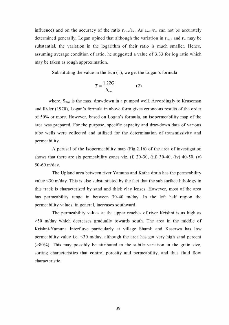
A perusal of the Isopermeability map (Fig.2.16) of the area of investigation
shows that there are six permeability zones viz. (i) 20-30, (iii) 30-40, (iv) 40-50, (v)
50-60 m/day.
The Upland area between river Yamuna and Katha drain has the permeability
value <30 m/day. This is also substantiated by the fact that the sub surface lithology in
this track is characterized by sand and thick clay lenses. However, most of the area
has permeability range in between 30-40 m/day. In the left half region the
permeability values, in general, increases southward.
The permeability values at the upper reaches of river Krishni is as high as
>50 m/day which decreases gradually towards south. The area in the middle of
Krishni-Yamuna Interfluve particularly at village Shamli and Kaserwa has low
permeability value i.e. <30 m/day, although the area has got very high sand percent
(>80%). This may possibly be attributed to the subtle variation in the grain size,
sorting characteristics that control porosity and permeability, and thus fluid flow
characteristic.
40
Fig.2.16 Logan’s Isopermeability map
2.7.2 Laboratory Estimation of Hydraulic Conductivity
Hydraulic conductivity (K) of an aquifer is known to depend both upon the fluid
properties and properties of transmitting medium. For the present study, seven aquifer
material (sand samples) were collected from drilling sites and their permeability was
determined using constant head Permeameter. Permeability can be obtained by measuring
the volume of water percolated through the sample of cross-sectional area A and length L
in given time t under a constant head h
From Darcy’s Law,
K=VL/hAt
at the laboratory temperature. The hydraulic conductivity obtained by Permeameter
ranges from 1.01 to 7.7 m/day which corresponds to typical conductivity value for fine to
medium grained sand. These values are lower than the pumping test value by several
orders. The depth range of the sand sample collected varies from 25-45 m which is less
than the aquifer tapped for pumping tests. The Pump tests were conducted at an average
depth of 143 m. The permeability of various aquifer materials is tabulated in Table 2.4.
41
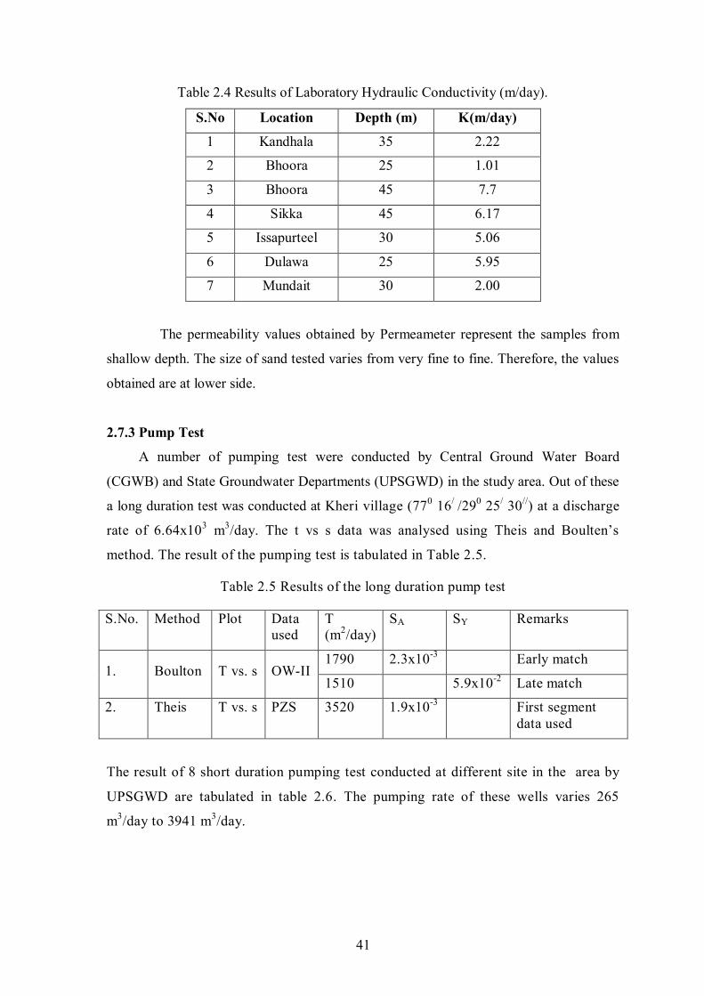
Table 2.4 Results of Laboratory Hydraulic Conductivity (m/day).
S.No Location Depth (m) K(m/day)
1 Kandhala 35 2.22
2 Bhoora 25 1.01
3 Bhoora 45 7.7
4 Sikka 45 6.17
5 Issapurteel 30 5.06
6 Dulawa 25 5.95
7 Mundait 30 2.00
The permeability values obtained by Permeameter represent the samples from
shallow depth. The size of sand tested varies from very fine to fine. Therefore, the values
obtained are at lower side.
2.7.3 Pump Test
A number of pumping test were conducted by Central Ground Water Board
(CGWB) and State Groundwater Departments (UPSGWD) in the study area. Out of these
a long duration test was conducted at Kheri village (770 16/ /290 25/ 30//) at a discharge
rate of 6.64x10³ m3/day. The t vs s data was analysed using Theis and Boulten’s
method. The result of the pumping test is tabulated in Table 2.5.
Table 2.5 Results of the long duration pump test
S.No. Method Plot Data used
T (m2/day)
SA SY Remarks
1. Boulton T vs. s OW-II 1790 2.3x10⁻³ Early match
1510 5.9x10⁻² Late match
2. Theis T vs. s PZS 3520 1.9x10⁻³ First segment data used
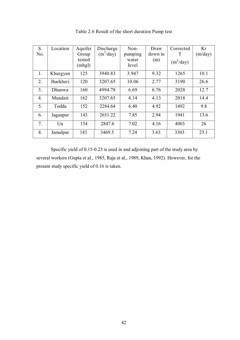
The result of 8 short duration pumping test conducted at different site in the area by
UPSGWD are tabulated in table 2.6. The pumping rate of these wells varies 265
m3/day to 3941 m3/day.
42
Table 2.6 Result of the short duration Pump test
S. No.
Location Aquifer Group tested (mbgl)
Discharge (m3/day)
Non-pumping
water level
Draw down in
(m)
Corrected T
(m2/day)
Kr (m/day)
1. Khurgyan 125 3940.83 3.947 9.32 1265 10.1
2. Jharkheri 120 3207.65 10.06 2.77 3190 26.6
3. Dhanwa 160 4994.78 6.69 6.76 2028 12.7
4. Mundait 162 3207.65 4.14 4.13 2018 14.4
5. Todda 152 2284.64 6.40 4.92 1492 9.8
6. Jaganpur 143 2651.22 7.85 2.94 1941 13.6
7. Un 154 2847.6 7.02 4.16 4003 26
8. Jamalpur 143 3469.5 7.24 3.63 3303 23.1
Specific yield of 0.15-0.23 is used in and adjoining part of the study area by
several workers (Gupta et al., 1985, Raja et al., 1989, Khan, 1992). However, for the
present study specific yield of 0.16 is taken.
43
3 - ESTIMATION OF DYNAMIC GROUNDWATER RESOURCE
3.1 Introduction
Quantification of the groundwater resource is a basic prerequisite for efficient
groundwater resource development and this is particularly vital for India with widely
prevalent semi-arid climate. The basic objective of groundwater resource evaluation is
to estimate the total quantity of groundwater resources available, and their future
supply potential to predict possible conflicts between supply and demand and to
provide a scientific database for rational water resources utilization (Earth Summit,
1992).
The effective groundwater budgets of an alluvial area require proper
understanding of the hydrodynamics of the basin. The heavy demand of groundwater
sometime leads to excessive withdrawals and indiscriminate utilization which is often
reflected in serious imbalance of hydrogeological situations at later date. It is therefore,
imperative to identify various recharges and discharge components of groundwater
regime and their effect on its variation with time.
3.2 Methodology
In the present study GEC 1997 methodology have been adopted with few
modifications, like subsurface flows and river-aquifer interaction have been estimated
with the help of groundwater flow model. The study area is divided in to canal
command area and non-command area for the assessment purpose (Fig.3.1).
Command area is the area which comes under major or medium surface water
irrigation. Contrarily, non-command areas lack any major or medium surface water
scheme. The groundwater fluctuation method is used for recharge assessment in the
monsoon season. The monsoon season is taken from June to October. The Kharif
crops (paddy, maize, fodder) are cultivated during this period. The rainfall recharge in
non-monsoon season is small component and hence estimated empirically. The non-
monsoon season is taken from November to May. The Rabi and Zaid (Wheat,
oilseeds, pulses etc.) crops are cultivated during this season. The value of specific
yield is taken from pumping test data, irrigation return flow, canal seepage and
surface water irrigation is estimated with the help of statistical data, field data and
recommended values for seepage etc. by GEC’97.
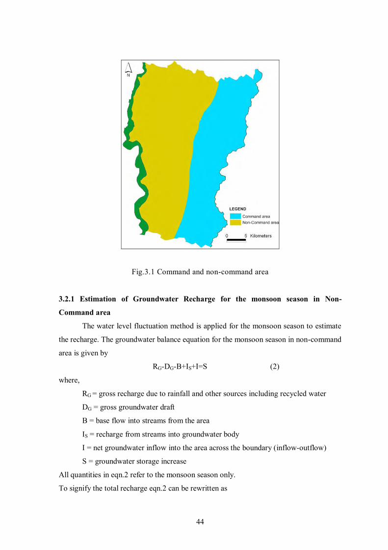
44
Fig.3.1 Command and non-command area
3.2.1 Estimation of Groundwater Recharge for the monsoon season in Non-
Command area
The water level fluctuation method is applied for the monsoon season to estimate
the recharge. The groundwater balance equation for the monsoon season in non-command
area is given by
RG-DG-B+IS+I=S (2)
where,
RG = gross recharge due to rainfall and other sources including recycled water
DG = gross groundwater draft
B = base flow into streams from the area
IS = recharge from streams into groundwater body
I = net groundwater inflow into the area across the boundary (inflow-outflow)
S = groundwater storage increase
All quantities in eqn.2 refer to the monsoon season only.
To signify the total recharge eqn.2 can be rewritten as
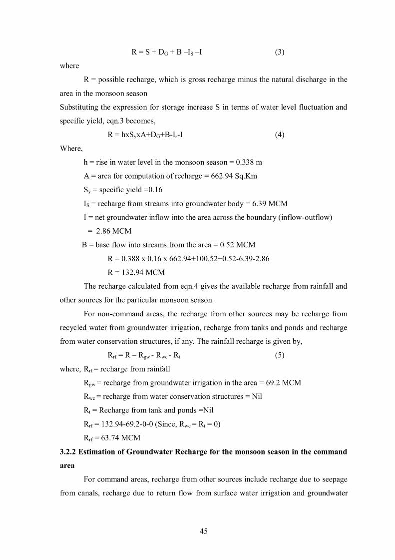
45
R = S + DG + B –IS –I (3)
where
R = possible recharge, which is gross recharge minus the natural discharge in the
area in the monsoon season
Substituting the expression for storage increase S in terms of water level fluctuation and
specific yield, eqn.3 becomes,
R = hxSyxA+DG+B-Is-I (4)
Where,
h = rise in water level in the monsoon season = 0.338 m
A = area for computation of recharge = 662.94 Sq.Km
Sy = specific yield =0.16
IS = recharge from streams into groundwater body = 6.39 MCM
I = net groundwater inflow into the area across the boundary (inflow-outflow)
= 2.86 MCM
B = base flow into streams from the area = 0.52 MCM
R = 0.388 x 0.16 x 662.94+100.52+0.52-6.39-2.86
R = 132.94 MCM
The recharge calculated from eqn.4 gives the available recharge from rainfall and
other sources for the particular monsoon season.
For non-command areas, the recharge from other sources may be recharge from
recycled water from groundwater irrigation, recharge from tanks and ponds and recharge
from water conservation structures, if any. The rainfall recharge is given by,
Rrf = R – Rgw - Rwc - Rt (5)
where, Rrf = recharge from rainfall
Rgw = recharge from groundwater irrigation in the area = 69.2 MCM
Rwc = recharge from water conservation structures = Nil
Rt = Recharge from tank and ponds =Nil
Rrf = 132.94-69.2-0-0 (Since, Rwc = Rt = 0)
Rrf = 63.74 MCM
3.2.2 Estimation of Groundwater Recharge for the monsoon season in the command
area
For command areas, recharge from other sources include recharge due to seepage
from canals, recharge due to return flow from surface water irrigation and groundwater
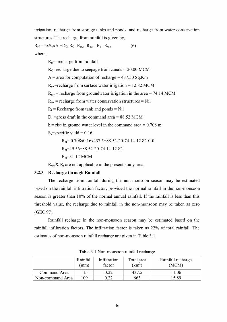
46
irrigation, recharge from storage tanks and ponds, and recharge from water conservation
structures. The recharge from rainfall is given by,
Rrf = hxSyxA +DG-RC- Rgw -Rsw - Rt– Rwc (6)
where,
Rrf = recharge from rainfall
RC=recharge due to seepage from canals = 20.00 MCM
A = area for computation of recharge = 437.50 Sq.Km
Rsw=recharge from surface water irrigation = 12.82 MCM
Rgw = recharge from groundwater irrigation in the area = 74.14 MCM
Rwc = recharge from water conservation structures = Nil
Rt = Recharge from tank and ponds = Nil
DG=gross draft in the command area = 88.52 MCM
h = rise in ground water level in the command area = 0.708 m
Sy=specific yield = 0.16
Rrf= 0.708x0.16x437.5+88.52-20-74.14-12.82-0-0
Rrf=49.56+88.52-20-74.14-12.82
Rrf=31.12 MCM
Rwc & Rt are not applicable in the present study area.
3.2.3 Recharge through Rainfall
The recharge from rainfall during the non-monsoon season may be estimated
based on the rainfall infiltration factor, provided the normal rainfall in the non-monsoon
season is greater than 10% of the normal annual rainfall. If the rainfall is less than this
threshold value, the recharge due to rainfall in the non-monsoon may be taken as zero
(GEC 97).
Rainfall recharge in the non-monsoon season may be estimated based on the
rainfall infiltration factors. The infiltration factor is taken as 22% of total rainfall. The
estimates of non-monsoon rainfall recharge are given in Table 3.1.
Table 3.1 Non-monsoon rainfall recharge
Rainfall (mm)
Infiltration factor
Total area (km2)
Rainfall recharge (MCM)
Command Area 115 0.22 437.5 11.06 Non-command Area 109 0.22 663 15.89
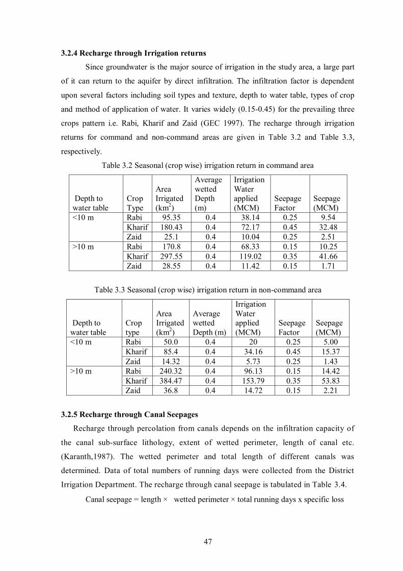
47
3.2.4 Recharge through Irrigation returns
Since groundwater is the major source of irrigation in the study area, a large part
of it can return to the aquifer by direct infiltration. The infiltration factor is dependent
upon several factors including soil types and texture, depth to water table, types of crop
and method of application of water. It varies widely (0.15-0.45) for the prevailing three
crops pattern i.e. Rabi, Kharif and Zaid (GEC 1997). The recharge through irrigation
returns for command and non-command areas are given in Table 3.2 and Table 3.3,
respectively.
Table 3.2 Seasonal (crop wise) irrigation return in command area
Depth to water table
Crop Type
Area Irrigated (km2)
Average wetted Depth (m)
Irrigation Water applied (MCM)
Seepage Factor
Seepage (MCM)
<10 m Rabi 95.35 0.4 38.14 0.25 9.54 Kharif 180.43 0.4 72.17 0.45 32.48 Zaid 25.1 0.4 10.04 0.25 2.51 >10 m Rabi 170.8 0.4 68.33 0.15 10.25 Kharif 297.55 0.4 119.02 0.35 41.66 Zaid 28.55 0.4 11.42 0.15 1.71
Table 3.3 Seasonal (crop wise) irrigation return in non-command area
Depth to water table
Crop type
Area Irrigated (km2)
Average wetted Depth (m)
Irrigation Water applied (MCM)
Seepage Factor
Seepage (MCM)
<10 m Rabi 50.0 0.4 20 0.25 5.00 Kharif 85.4 0.4 34.16 0.45 15.37 Zaid 14.32 0.4 5.73 0.25 1.43 >10 m Rabi 240.32 0.4 96.13 0.15 14.42 Kharif 384.47 0.4 153.79 0.35 53.83 Zaid 36.8 0.4 14.72 0.15 2.21
3.2.5 Recharge through Canal Seepages
Recharge through percolation from canals depends on the infiltration capacity of
the canal sub-surface lithology, extent of wetted perimeter, length of canal etc.
(Karanth,1987). The wetted perimeter and total length of different canals was
determined. Data of total numbers of running days were collected from the District
Irrigation Department. The recharge through canal seepage is tabulated in Table 3.4.
Canal seepage = length × wetted perimeter × total running days x specific loss
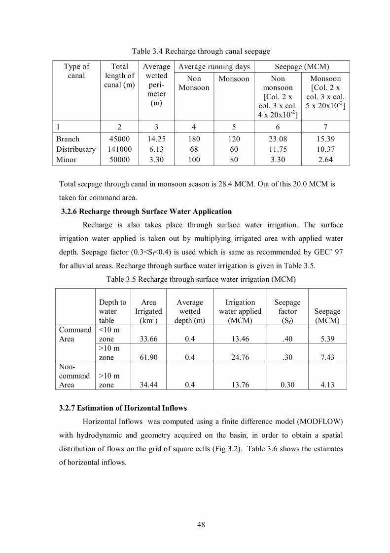
48
Table 3.4 Recharge through canal seepage
Type of canal
Total length of canal (m)
Average wetted peri-meter (m)
Average running days Seepage (MCM) Non
Monsoon Monsoon Non
monsoon [Col. 2 x
col. 3 x col. 4 x 20x10-2]
Monsoon [Col. 2 x
col. 3 x col. 5 x 20x10-2]
1 2 3 4 5 6 7 Branch Distributary Minor
45000 141000 50000
14.25 6.13 3.30
180 68
100
120 60 80
23.08 11.75 3.30
15.39 10.37 2.64
Total seepage through canal in monsoon season is 28.4 MCM. Out of this 20.0 MCM is
taken for command area.
3.2.6 Recharge through Surface Water Application
Recharge is also takes place through surface water irrigation. The surface
irrigation water applied is taken out by multiplying irrigated area with applied water
depth. Seepage factor (0.3<Sf<0.4) is used which is same as recommended by GEC’ 97
for alluvial areas. Recharge through surface water irrigation is given in Table 3.5.
Table 3.5 Recharge through surface water irrigation (MCM)
Depth to water table
Area Irrigated
(km2)
Average wetted
depth (m)
Irrigation water applied
(MCM)
Seepage factor (Sf)
Seepage (MCM)
Command Area
<10 m zone 33.66 0.4 13.46 .40 5.39 >10 m zone 61.90 0.4 24.76 .30 7.43
Non-command Area
>10 m zone 34.44 0.4 13.76 0.30 4.13
3.2.7 Estimation of Horizontal Inflows
Horizontal Inflows was computed using a finite difference model (MODFLOW)
with hydrodynamic and geometry acquired on the basin, in order to obtain a spatial
distribution of flows on the grid of square cells (Fig 3.2). Table 3.6 shows the estimates
of horizontal inflows.
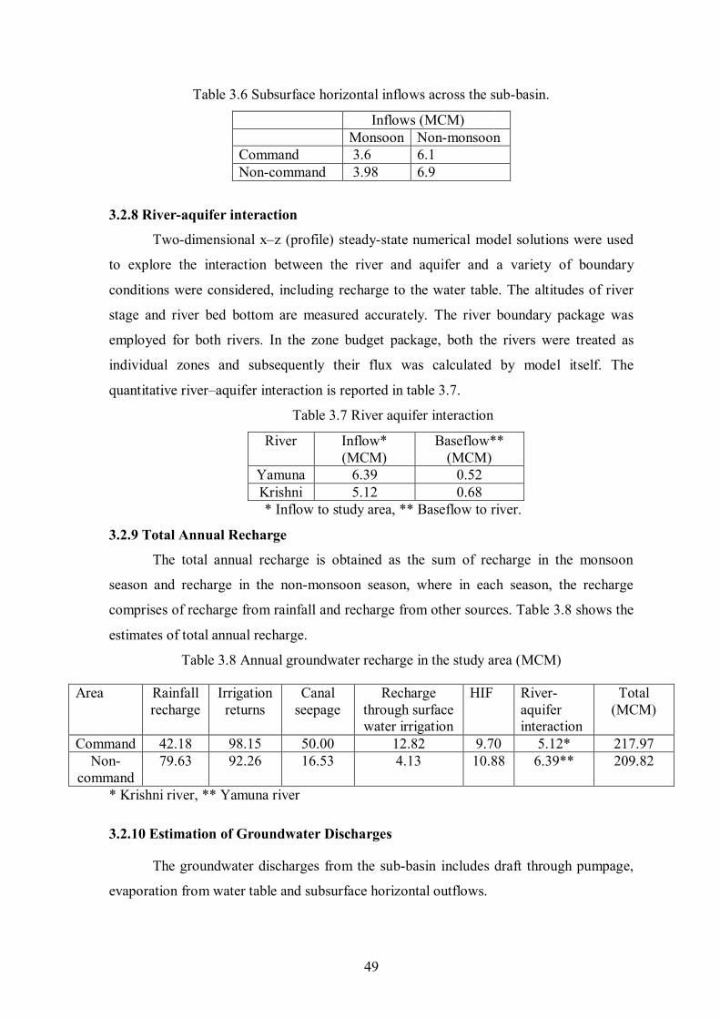
49
Table 3.6 Subsurface horizontal inflows across the sub-basin.
Inflows (MCM) Monsoon Non-monsoon Command 3.6 6.1 Non-command 3.98 6.9
3.2.8 River-aquifer interaction
Two-dimensional x–z (profile) steady-state numerical model solutions were used
to explore the interaction between the river and aquifer and a variety of boundary
conditions were considered, including recharge to the water table. The altitudes of river
stage and river bed bottom are measured accurately. The river boundary package was
employed for both rivers. In the zone budget package, both the rivers were treated as
individual zones and subsequently their flux was calculated by model itself. The
quantitative river–aquifer interaction is reported in table 3.7.
Table 3.7 River aquifer interaction
River Inflow* (MCM)
Baseflow** (MCM)
Yamuna 6.39 0.52 Krishni 5.12 0.68 * Inflow to study area, ** Baseflow to river.
3.2.9 Total Annual Recharge
The total annual recharge is obtained as the sum of recharge in the monsoon
season and recharge in the non-monsoon season, where in each season, the recharge
comprises of recharge from rainfall and recharge from other sources. Table 3.8 shows the
estimates of total annual recharge.
Table 3.8 Annual groundwater recharge in the study area (MCM)
Area Rainfall recharge
Irrigation returns
Canal seepage
Recharge through surface water irrigation
HIF River-aquifer interaction
Total (MCM)
Command 42.18 98.15 50.00 12.82 9.70 5.12* 217.97 Non-
command 79.63 92.26 16.53 4.13 10.88 6.39** 209.82
* Krishni river, ** Yamuna river
3.2.10 Estimation of Groundwater Discharges
The groundwater discharges from the sub-basin includes draft through pumpage,
evaporation from water table and subsurface horizontal outflows.
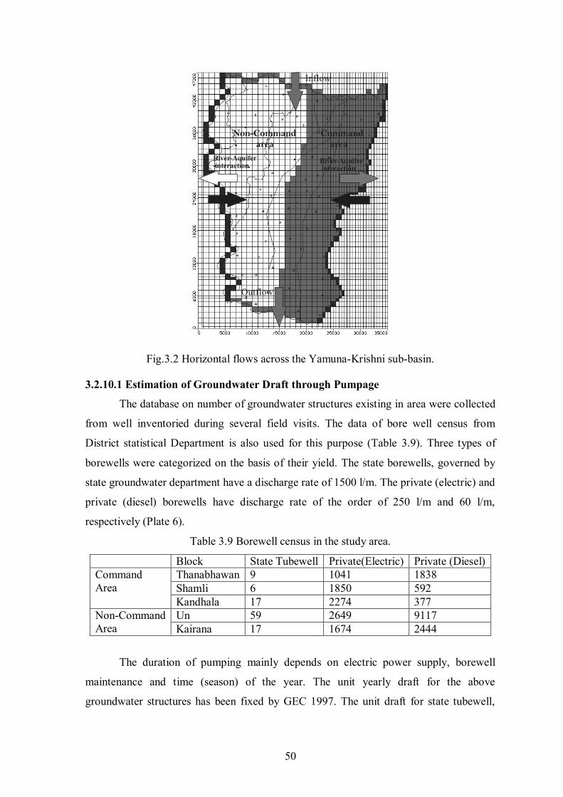
50
Command area
Non-Command area
River-Aquifer interaction River-Aquifer
interaction
Inflow
Outflow
Fig.3.2 Horizontal flows across the Yamuna-Krishni sub-basin.
3.2.10.1 Estimation of Groundwater Draft through Pumpage
The database on number of groundwater structures existing in area were collected
from well inventoried during several field visits. The data of bore well census from
District statistical Department is also used for this purpose (Table 3.9). Three types of
borewells were categorized on the basis of their yield. The state borewells, governed by
state groundwater department have a discharge rate of 1500 l/m. The private (electric) and
private (diesel) borewells have discharge rate of the order of 250 l/m and 60 l/m,
respectively (Plate 6).
Table 3.9 Borewell census in the study area.
Block State Tubewell Private(Electric) Private (Diesel) Command Area
Thanabhawan 9 1041 1838 Shamli 6 1850 592 Kandhala 17 2274 377
Non-Command Area
Un 59 2649 9117 Kairana 17 1674 2444
The duration of pumping mainly depends on electric power supply, borewell
maintenance and time (season) of the year. The unit yearly draft for the above
groundwater structures has been fixed by GEC 1997. The unit draft for state tubewell,
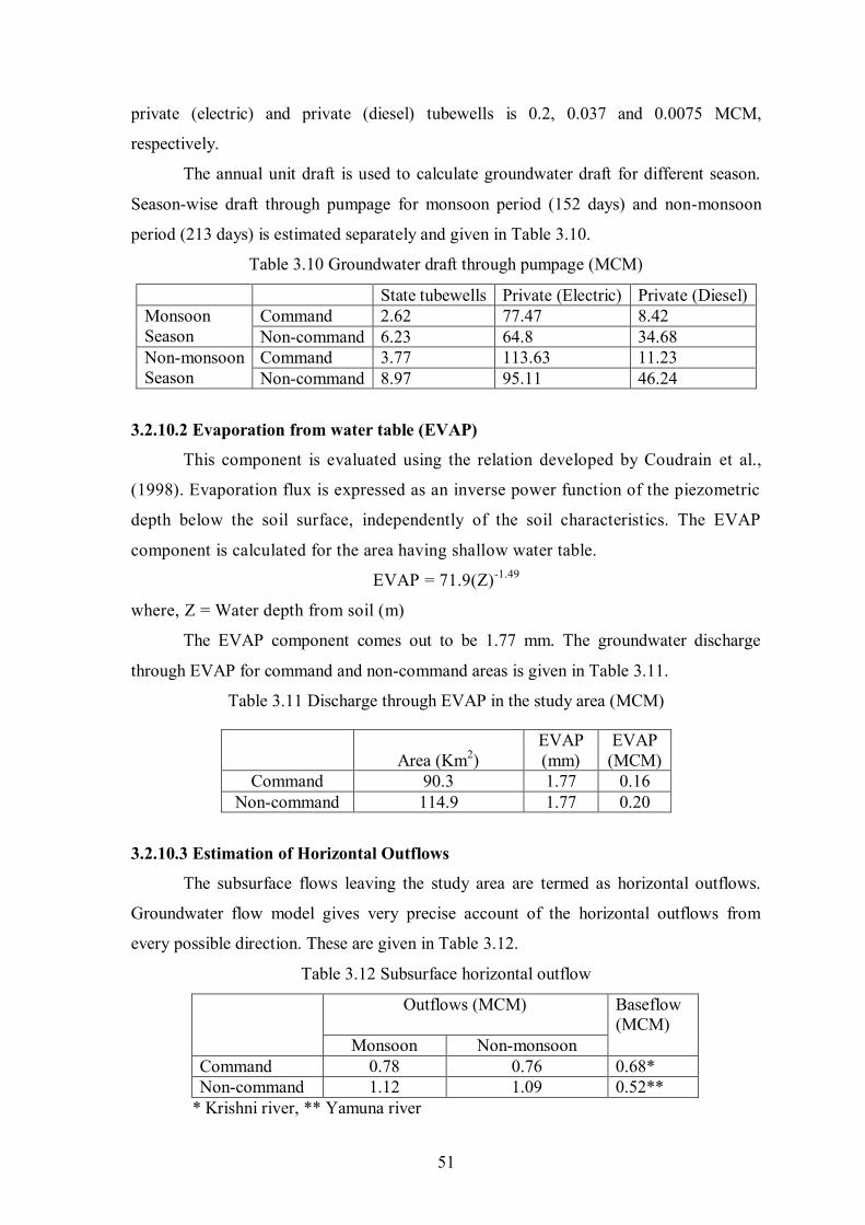
51
private (electric) and private (diesel) tubewells is 0.2, 0.037 and 0.0075 MCM,
respectively.
The annual unit draft is used to calculate groundwater draft for different season.
Season-wise draft through pumpage for monsoon period (152 days) and non-monsoon
period (213 days) is estimated separately and given in Table 3.10.
Table 3.10 Groundwater draft through pumpage (MCM)
State tubewells Private (Electric) Private (Diesel) Monsoon Season
Command 2.62 77.47 8.42 Non-command 6.23 64.8 34.68
Non-monsoon Season
Command 3.77 113.63 11.23 Non-command 8.97 95.11 46.24
3.2.10.2 Evaporation from water table (EVAP)
This component is evaluated using the relation developed by Coudrain et al.,
(1998). Evaporation flux is expressed as an inverse power function of the piezometric
depth below the soil surface, independently of the soil characteristics. The EVAP
component is calculated for the area having shallow water table.
EVAP = 71.9(Z)-1.49
where, Z = Water depth from soil (m)
The EVAP component comes out to be 1.77 mm. The groundwater discharge
through EVAP for command and non-command areas is given in Table 3.11.
Table 3.11 Discharge through EVAP in the study area (MCM)
Area (Km2) EVAP (mm)
EVAP (MCM)
Command 90.3 1.77 0.16 Non-command 114.9 1.77 0.20
3.2.10.3 Estimation of Horizontal Outflows
The subsurface flows leaving the study area are termed as horizontal outflows.
Groundwater flow model gives very precise account of the horizontal outflows from
every possible direction. These are given in Table 3.12.
Table 3.12 Subsurface horizontal outflow
Outflows (MCM)
Baseflow (MCM)
Monsoon Non-monsoon Command 0.78 0.76 0.68* Non-command 1.12 1.09 0.52**
* Krishni river, ** Yamuna river
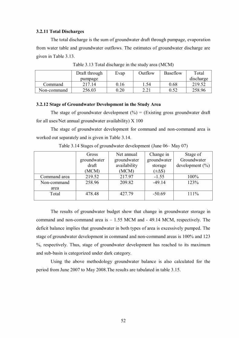
52
3.2.11 Total Discharges
The total discharge is the sum of groundwater draft through pumpage, evaporation
from water table and groundwater outflows. The estimates of groundwater discharge are
given in Table 3.13.
Table 3.13 Total discharge in the study area (MCM)
Draft through pumpage
Evap Outflow Baseflow Total discharge
Command 217.14 0.16 1.54 0.68 219.52 Non-command 256.03 0.20 2.21 0.52 258.96
3.2.12 Stage of Groundwater Development in the Study Area
The stage of groundwater development (%) = (Existing gross groundwater draft
for all uses/Net annual groundwater availability) X 100
The stage of groundwater development for command and non-command area is
worked out separately and is given in Table 3.14.
Table 3.14 Stages of groundwater development (June 06– May 07)
Gross groundwater
draft (MCM)
Net annual groundwater availability
(MCM)
Change in groundwater
storage (±ΔS)
Stage of Groundwater
development (%)
Command area 219.52 217.97 -1.55 100% Non-command
area 258.96 209.82 -49.14 123%
Total 478.48 427.79 -50.69 111%
The results of groundwater budget show that change in groundwater storage in
command and non-command area is – 1.55 MCM and - 49.14 MCM, respectively. The
deficit balance implies that groundwater in both types of area is excessively pumped. The
stage of groundwater development in command and non-command areas is 100% and 123
%, respectively. Thus, stage of groundwater development has reached to its maximum
and sub-basin is categorized under dark category.
Using the above methodology groundwater balance is also calculated for the
period from June 2007 to May 2008.The results are tabulated in table 3.15.
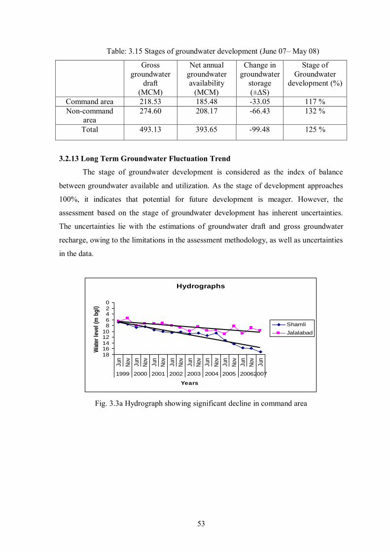
53
Table: 3.15 Stages of groundwater development (June 07– May 08)
Gross groundwater
draft (MCM)
Net annual groundwater availability
(MCM)
Change in groundwater
storage (±ΔS)
Stage of Groundwater
development (%)
Command area 218.53 185.48 -33.05 117 % Non-command
area 274.60 208.17 -66.43 132 %
Total 493.13 393.65 -99.48 125 %
3.2.13 Long Term Groundwater Fluctuation Trend
The stage of groundwater development is considered as the index of balance
between groundwater available and utilization. As the stage of development approaches
100%, it indicates that potential for future development is meager. However, the
assessment based on the stage of groundwater development has inherent uncertainties.
The uncertainties lie with the estimations of groundwater draft and gross groundwater
recharge, owing to the limitations in the assessment methodology, as well as uncertainties
in the data.
Hydrographs
02468
1012141618
Jun
Nov
Jun
Nov
Jun
Nov
Jun
Nov
Jun
Nov
Jun
Nov
Jun
Nov
Jun
Nov
Jun
1999 2000 2001 2002 2003 2004 2005 20062007
Years
Wat
er l
evel
(m
bg
l)
Shamli
Jalalabad
Fig. 3.3a Hydrograph showing significant decline in command area
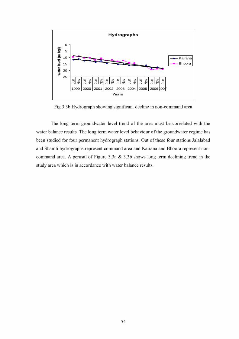
54
Hydrographs
0
5
10
15
20
25
Jun
Nov
Jun
Nov
Jun
Nov
Jun
Nov
Jun
Nov
Jun
Nov
Jun
Nov
Jun
Nov
Jun
1999 2000 2001 2002 2003 2004 2005 20062007
Years
Wat
er l
evel
(m
bg
l)Kairana
Bhoora
Fig.3.3b Hydrograph showing significant decline in non-command area
The long term groundwater level trend of the area must be correlated with the
water balance results. The long term water level behaviour of the groundwater regime has
been studied for four permanent hydrograph stations. Out of these four stations Jalalabad
and Shamli hydrographs represent command area and Kairana and Bhoora represent non-
command area. A perusal of Figure 3.3a & 3.3b shows long term declining trend in the
study area which is in accordance with water balance results.
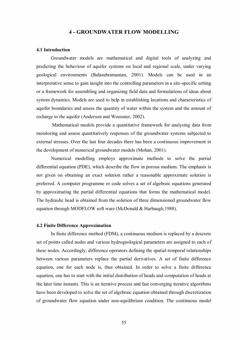
55
4 - GROUNDWATER FLOW MODELLING
4.1 Introduction
Groundwater models are mathematical and digital tools of analyzing and
predicting the behaviour of aquifer systems on local and regional scale, under varying
geological environments (Balasubramanian, 2001). Models can be used in an
interpretative sense to gain insight into the controlling parameters in a site-specific setting
or a framework for assembling and organizing field data and formulations of ideas about
system dynamics. Models are used to help in establishing locations and characteristics of
aquifer boundaries and assess the quantity of water within the system and the amount of
recharge to the aquifer (Anderson and Woessner, 2002).
Mathematical models provide a quantitative framework for analysing data from
monitoring and assess quantitatively responses of the groundwater systems subjected to
external stresses. Over the last four decades there has been a continuous improvement in
the development of numerical groundwater models (Mohan, 2001).
Numerical modelling employs approximate methods to solve the partial
differential equation (PDE), which describe the flow in porous medium. The emphasis is
not given on obtaining an exact solution rather a reasonable approximate solution is
preferred. A computer programme or code solves a set of algebraic equations generated
by approximating the partial differential equations that forms the mathematical model.
The hydraulic head is obtained from the solution of three dimensioned groundwater flow
equation through MODFLOW soft ware (McDonald & Harbaugh,1988).
4.2 Finite Difference Approximation
In finite difference method (FDM), a continuous medium is replaced by a descrete
set of points called nodes and various hydrogeological parameters are assigned to each of
these nodes. Accordingly, difference operators defining the spatial-temporal relationships
between various parameters replace the partial derivatives. A set of finite difference
equation, one for each node is, thus obtained. In order to solve a finite difference
equation, one has to start with the initial distribution of heads and computation of heads at
the later time instants. This is an iterative process and fast converging iterative algorithms
have been developed to solve the set of algebraic equation obtained through discretization
of groundwater flow equation under non-equilibrium condition. The continuous model
56
can be replaced with a set of discrete point arranged in a grid pattern. This pattern more
often known as finite difference grid. The general flow equation for unsteady flow of
groundwater in confined condition in the horizontal direction
qt
hS
y
hT
hyyx
xT
2
2
2
2
( 1 )
When eqn (1) is applied to an unconfined aquifer, the Dupuit assumptions are
used: (1) flow lines are horizonatal and equipotential lines are vertical and (2) the
horizontal hydraulic gradient is equal to the slope of the free surface and is invariant with
depth. It is understood that hKT xx and hKT yy , where h is the elevation of water
table above the bottom of the aquifer.
Rt
hS
z
hK
y
hK
x
hK szyx
2
2
2
2
2
2
( 2 )
Where xK , yK and zK are components of the hydraulic conductivity tensor. sS is
the Specific storage, R is general sink/source term that is intrinsically positive and
defines the volume of inflow to the system per unit volume of aquifer per unit of time.
4.3 Model conceptualization and data acquisition
The purpose of building a conceptual model is to simplify the field problem and
organize the associated field data so that the system can be analyzed more readily
(Anderson and Woessner, 2002). The conceptualization include synthesis and framing up
of data pertaining to geology, hydrogeology, hydrology, and meteorology.
4.3.1 Groundwater Level Data
A network of 60 existing observation wells were selected for water level
monitoring. The water level monitoring programme was initiated in November 2005. The
depth of monitoring wells ranged between 10-30 m and these tap the first layer of the
aquifer. Water levels were recorded from November 2005 to November 2007 at all
observation points. Care was taken to try and obtain static groundwater levels however
errors may have been introduced because practically it was impossible to stop all
pumping in an extensively cultivated area where concentration of groundwater abstraction
structures are so high.
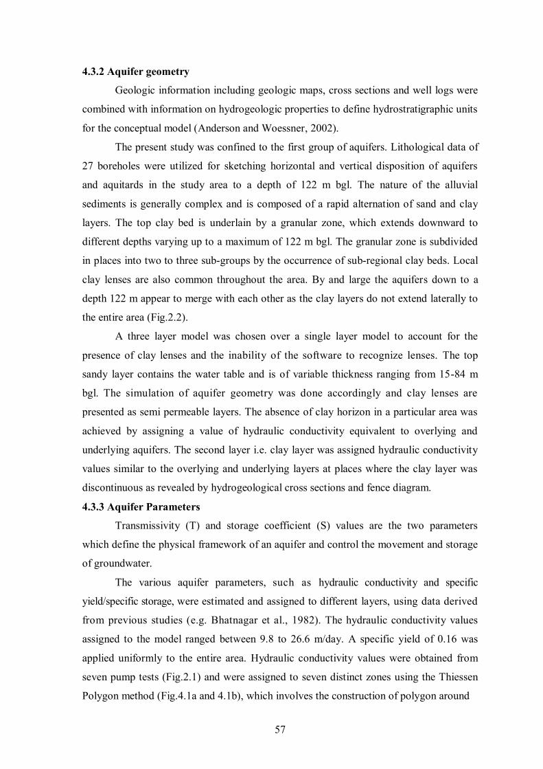
57
4.3.2 Aquifer geometry
Geologic information including geologic maps, cross sections and well logs were
combined with information on hydrogeologic properties to define hydrostratigraphic units
for the conceptual model (Anderson and Woessner, 2002).
The present study was confined to the first group of aquifers. Lithological data of
27 boreholes were utilized for sketching horizontal and vertical disposition of aquifers
and aquitards in the study area to a depth of 122 m bgl. The nature of the alluvial
sediments is generally complex and is composed of a rapid alternation of sand and clay
layers. The top clay bed is underlain by a granular zone, which extends downward to
different depths varying up to a maximum of 122 m bgl. The granular zone is subdivided
in places into two to three sub-groups by the occurrence of sub-regional clay beds. Local
clay lenses are also common throughout the area. By and large the aquifers down to a
depth 122 m appear to merge with each other as the clay layers do not extend laterally to
the entire area (Fig.2.2).
A three layer model was chosen over a single layer model to account for the
presence of clay lenses and the inability of the software to recognize lenses. The top
sandy layer contains the water table and is of variable thickness ranging from 15-84 m
bgl. The simulation of aquifer geometry was done accordingly and clay lenses are
presented as semi permeable layers. The absence of clay horizon in a particular area was
achieved by assigning a value of hydraulic conductivity equivalent to overlying and
underlying aquifers. The second layer i.e. clay layer was assigned hydraulic conductivity
values similar to the overlying and underlying layers at places where the clay layer was
discontinuous as revealed by hydrogeological cross sections and fence diagram.
4.3.3 Aquifer Parameters
Transmissivity (T) and storage coefficient (S) values are the two parameters
which define the physical framework of an aquifer and control the movement and storage
of groundwater.
The various aquifer parameters, such as hydraulic conductivity and specific
yield/specific storage, were estimated and assigned to different layers, using data derived
from previous studies (e.g. Bhatnagar et al., 1982). The hydraulic conductivity values
assigned to the model ranged between 9.8 to 26.6 m/day. A specific yield of 0.16 was
applied uniformly to the entire area. Hydraulic conductivity values were obtained from
seven pump tests (Fig.2.1) and were assigned to seven distinct zones using the Thiessen
Polygon method (Fig.4.1a and 4.1b), which involves the construction of polygon around
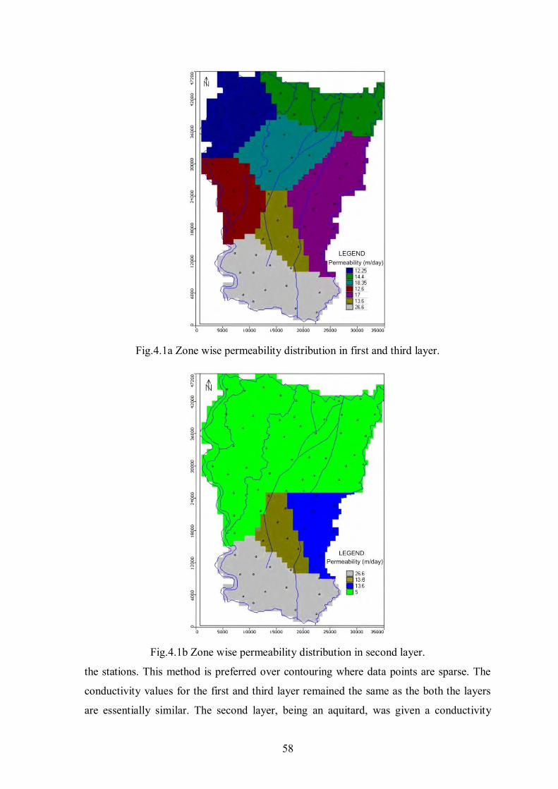
58
Fig.4.1a Zone wise permeability distribution in first and third layer.
Fig.4.1b Zone wise permeability distribution in second layer.
the stations. This method is preferred over contouring where data points are sparse. The
conductivity values for the first and third layer remained the same as the both the layers
are essentially similar. The second layer, being an aquitard, was given a conductivity
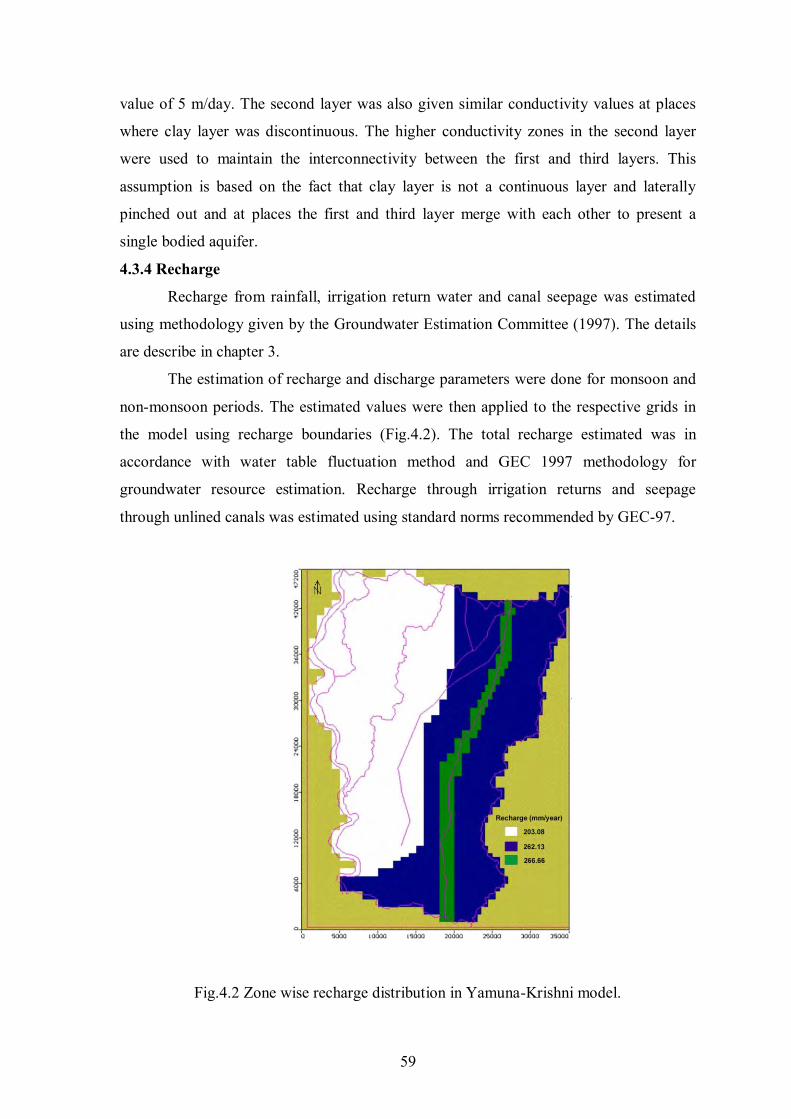
59
value of 5 m/day. The second layer was also given similar conductivity values at places
where clay layer was discontinuous. The higher conductivity zones in the second layer
were used to maintain the interconnectivity between the first and third layers. This
assumption is based on the fact that clay layer is not a continuous layer and laterally
pinched out and at places the first and third layer merge with each other to present a
single bodied aquifer.
4.3.4 Recharge
Recharge from rainfall, irrigation return water and canal seepage was estimated
using methodology given by the Groundwater Estimation Committee (1997). The details
are describe in chapter 3.
The estimation of recharge and discharge parameters were done for monsoon and
non-monsoon periods. The estimated values were then applied to the respective grids in
the model using recharge boundaries (Fig.4.2). The total recharge estimated was in
accordance with water table fluctuation method and GEC 1997 methodology for
groundwater resource estimation. Recharge through irrigation returns and seepage
through unlined canals was estimated using standard norms recommended by GEC-97.
Fig.4.2 Zone wise recharge distribution in Yamuna-Krishni model.
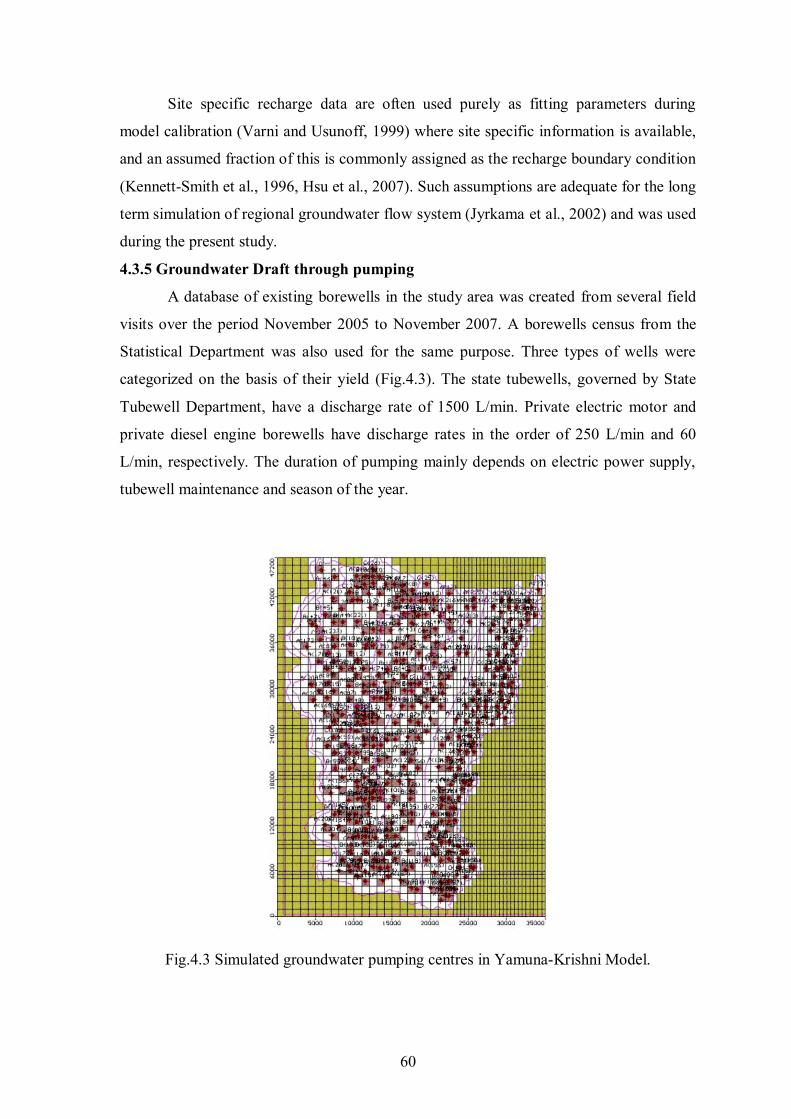
60
Site specific recharge data are often used purely as fitting parameters during
model calibration (Varni and Usunoff, 1999) where site specific information is available,
and an assumed fraction of this is commonly assigned as the recharge boundary condition
(Kennett-Smith et al., 1996, Hsu et al., 2007). Such assumptions are adequate for the long
term simulation of regional groundwater flow system (Jyrkama et al., 2002) and was used
during the present study.
4.3.5 Groundwater Draft through pumping
A database of existing borewells in the study area was created from several field
visits over the period November 2005 to November 2007. A borewells census from the
Statistical Department was also used for the same purpose. Three types of wells were
categorized on the basis of their yield (Fig.4.3). The state tubewells, governed by State
Tubewell Department, have a discharge rate of 1500 L/min. Private electric motor and
private diesel engine borewells have discharge rates in the order of 250 L/min and 60
L/min, respectively. The duration of pumping mainly depends on electric power supply,
tubewell maintenance and season of the year.
Fig.4.3 Simulated groundwater pumping centres in Yamuna-Krishni Model.
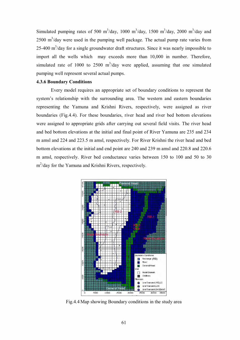
61
Simulated pumping rates of 500 m3/day, 1000 m3/day, 1500 m3/day, 2000 m3/day and
2500 m3/day were used in the pumping well package. The actual pump rate varies from
25-400 m3/day for a single groundwater draft structures. Since it was nearly impossible to
import all the wells which may exceeds more than 10,000 in number. Therefore,
simulated rate of 1000 to 2500 m3/day were applied, assuming that one simulated
pumping well represent several actual pumps.
4.3.6 Boundary Conditions
Every model requires an appropriate set of boundary conditions to represent the
system’s relationship with the surrounding area. The western and eastern boundaries
representing the Yamuna and Krishni Rivers, respectively, were assigned as river
boundaries (Fig.4.4). For these boundaries, river head and river bed bottom elevations
were assigned to appropriate grids after carrying out several field visits. The river head
and bed bottom elevations at the initial and final point of River Yamuna are 235 and 234
m amsl and 224 and 223.5 m amsl, respectively. For River Krishni the river head and bed
bottom elevations at the initial and end point are 240 and 239 m amsl and 220.8 and 220.6
m amsl, respectively. River bed conductance varies between 150 to 100 and 50 to 30
m2/day for the Yamuna and Krishni Rivers, respectively.
Fig.4.4 Map showing Boundary conditions in the study area
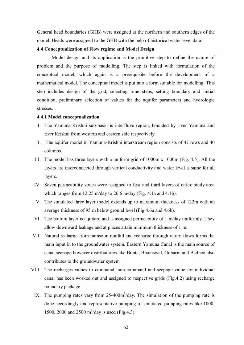
62
General head boundaries (GHB) were assigned at the northern and southern edges of the
model. Heads were assigned to the GHB with the help of historical water level data.
4.4 Conceptualization of Flow regime and Model Design
Model design and its application is the primitive step to define the nature of
problem and the purpose of modelling. The step is linked with formulation of the
conceptual model, which again is a prerequisite before the development of a
mathematical model. The conceptual model is put into a form suitable for modelling. This
step includes design of the grid, selecting time steps, setting boundary and initial
condition, preliminary selection of values for the aquifer parameters and hydrologic
stresses.
4.4.1 Model conceptualization
I. The Yamuna-Krishni sub-basin is interfluve region, bounded by river Yamuna and
river Krishni from western and eastern side respectively.
II. The aquifer model in Yamuna-Krishni interstream region consists of 47 rows and 40
columns.
III. The model has three layers with a uniform grid of 1000m x 1000m (Fig. 4.5). All the
layers are interconnected through vertical conductivity and water level is same for all
layers.
IV. Seven permeability zones were assigned to first and third layers of entire study area
which ranges from 12.25 m/day to 26.6 m/day (Fig. 4.1a and 4.1b).
V. The simulated three layer model extends up to maximum thickness of 122m with an
average thickness of 95 m below ground level (Fig.4.6a and 4.6b).
VI. The bottom layer is aquitard and is assigned permeability of 1 m/day uniformly. They
allow downward leakage and at places attain minimum thickness of 1 m.
VII. Natural recharge from monsoon rainfall and recharge through return flows forms the
main input in to the groundwater system. Eastern Yamuna Canal is the main source of
canal seepage however distributaries like Bunta, Bhainswal, Goharni and Badheo also
contributes to the groundwater system.
VIII. The recharges values to command, non-command and seepage value for individual
canal has been worked out and assigned to respective grids (Fig.4.2) using recharge
boundary package.
IX. The pumping rates vary from 25-400m3/day. The simulation of the pumping rate is
done accordingly and representative pumping of simulated pumping rates like 1000,
1500, 2000 and 2500 m3/day is used (Fig.4.3).
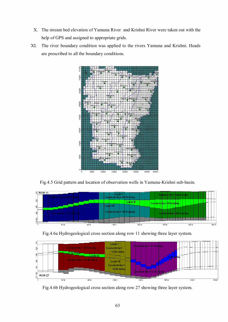
63
X. The stream bed elevation of Yamuna River and Krishni River were taken out with the
help of GPS and assigned to appropriate grids.
XI. The river boundary condition was applied to the rivers Yamuna and Krishni. Heads
are prescribed to all the boundary conditions.
Fig.4.5 Grid pattern and location of observation wells in Yamuna-Krishni sub-basin.
Fig.4.6a Hydrogeological cross section along row 11 showing three layer system.
Fig.4.6b Hydrogeological cross section along row 27 showing three layer system.
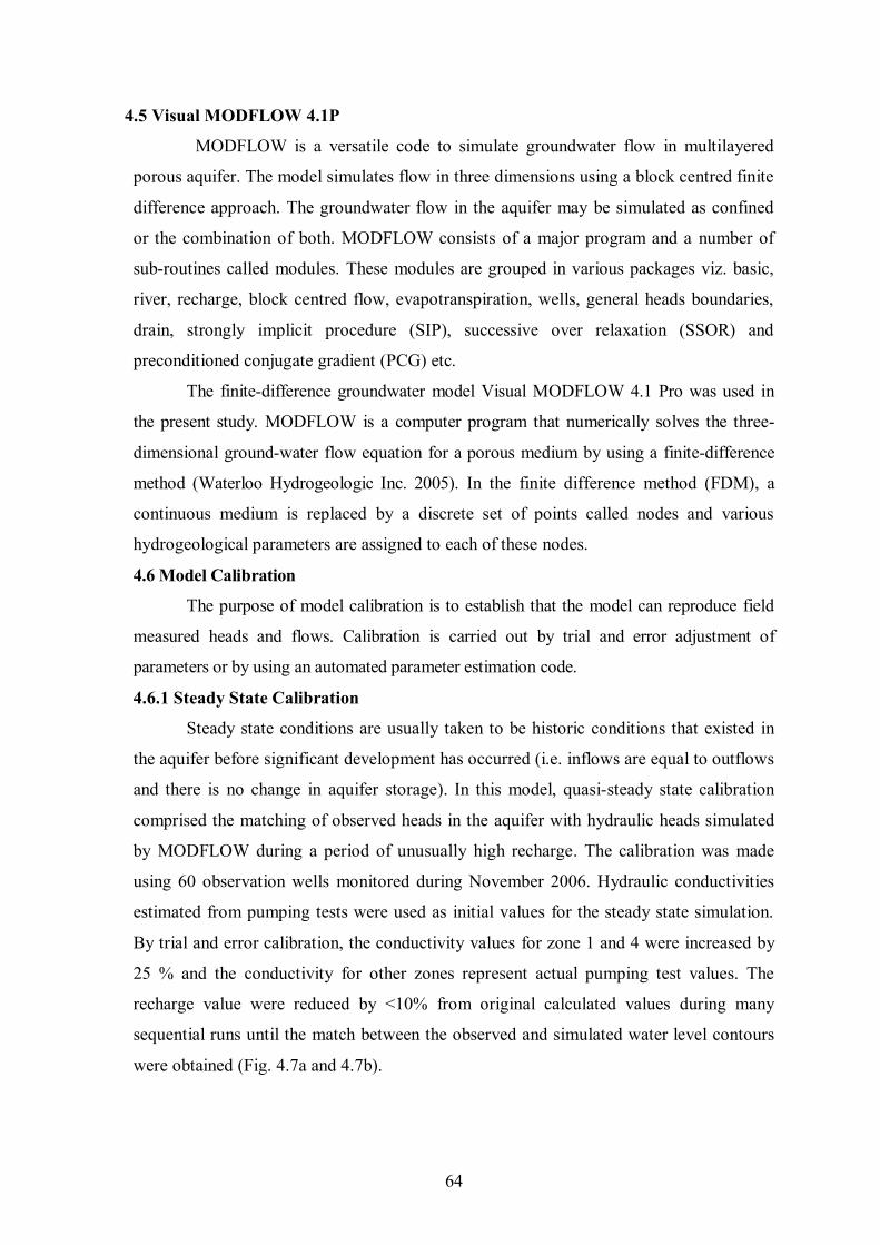
64
4.5 Visual MODFLOW 4.1P
MODFLOW is a versatile code to simulate groundwater flow in multilayered
porous aquifer. The model simulates flow in three dimensions using a block centred finite
difference approach. The groundwater flow in the aquifer may be simulated as confined
or the combination of both. MODFLOW consists of a major program and a number of
sub-routines called modules. These modules are grouped in various packages viz. basic,
river, recharge, block centred flow, evapotranspiration, wells, general heads boundaries,
drain, strongly implicit procedure (SIP), successive over relaxation (SSOR) and
preconditioned conjugate gradient (PCG) etc.
The finite-difference groundwater model Visual MODFLOW 4.1 Pro was used in
the present study. MODFLOW is a computer program that numerically solves the three-
dimensional ground-water flow equation for a porous medium by using a finite-difference
method (Waterloo Hydrogeologic Inc. 2005). In the finite difference method (FDM), a
continuous medium is replaced by a discrete set of points called nodes and various
hydrogeological parameters are assigned to each of these nodes.
4.6 Model Calibration
The purpose of model calibration is to establish that the model can reproduce field
measured heads and flows. Calibration is carried out by trial and error adjustment of
parameters or by using an automated parameter estimation code.
4.6.1 Steady State Calibration
Steady state conditions are usually taken to be historic conditions that existed in
the aquifer before significant development has occurred (i.e. inflows are equal to outflows
and there is no change in aquifer storage). In this model, quasi-steady state calibration
comprised the matching of observed heads in the aquifer with hydraulic heads simulated
by MODFLOW during a period of unusually high recharge. The calibration was made
using 60 observation wells monitored during November 2006. Hydraulic conductivities
estimated from pumping tests were used as initial values for the steady state simulation.
By trial and error calibration, the conductivity values for zone 1 and 4 were increased by
25 % and the conductivity for other zones represent actual pumping test values. The
recharge value were reduced by <10% from original calculated values during many
sequential runs until the match between the observed and simulated water level contours
were obtained (Fig. 4.7a and 4.7b).
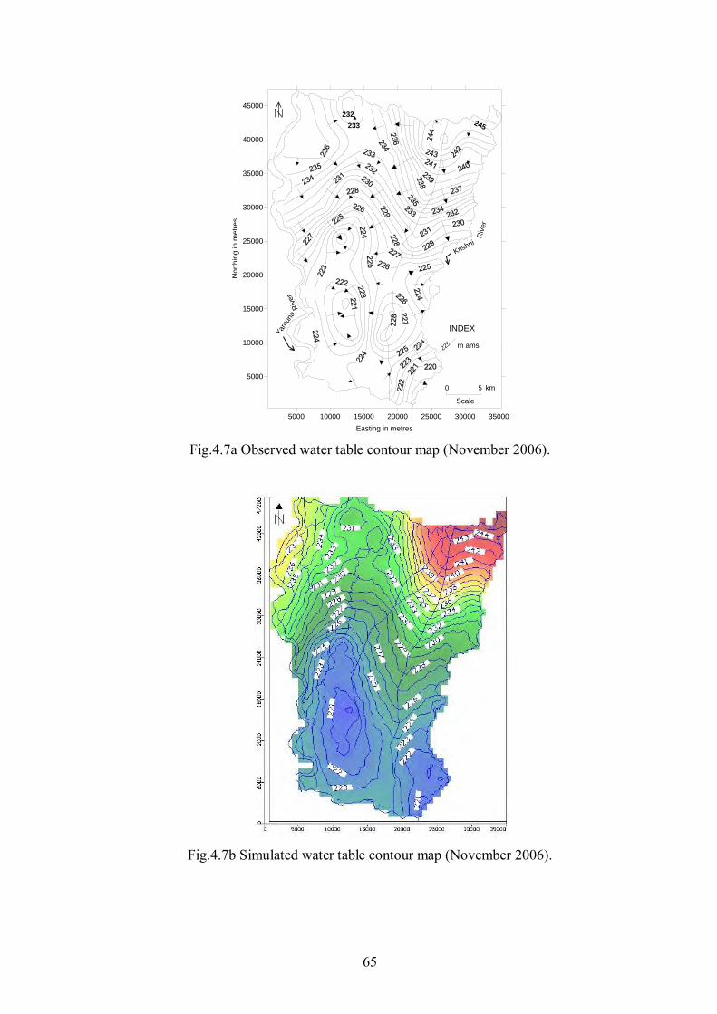
65
5000 10000 15000 20000 25000 30000 35000
Easting in metres
5000
10000
15000
20000
25000
30000
35000
40000
45000
Nort
hin
g in m
etr
es
Krishni
Riv
er
Yam
una
Riv
er
0 5 km
225 m amsl
INDEX
233
232245
Scale
Fig.4.7a Observed water table contour map (November 2006).
Fig.4.7b Simulated water table contour map (November 2006).
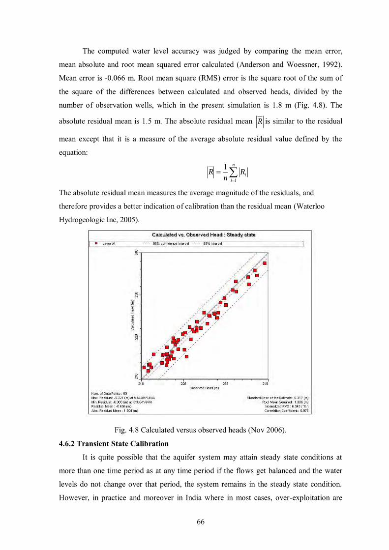
66
The computed water level accuracy was judged by comparing the mean error,
mean absolute and root mean squared error calculated (Anderson and Woessner, 1992).
Mean error is -0.066 m. Root mean square (RMS) error is the square root of the sum of
the square of the differences between calculated and observed heads, divided by the
number of observation wells, which in the present simulation is 1.8 m (Fig. 4.8). The
absolute residual mean is 1.5 m. The absolute residual mean R is similar to the residual
mean except that it is a measure of the average absolute residual value defined by the
equation:
n
i
iRn
R1
1
The absolute residual mean measures the average magnitude of the residuals, and
therefore provides a better indication of calibration than the residual mean (Waterloo
Hydrogeologic Inc, 2005).
Fig. 4.8 Calculated versus observed heads (Nov 2006).
4.6.2 Transient State Calibration
It is quite possible that the aquifer system may attain steady state conditions at
more than one time period as at any time period if the flows get balanced and the water
levels do not change over that period, the system remains in the steady state condition.
However, in practice and moreover in India where in most cases, over-exploitation are
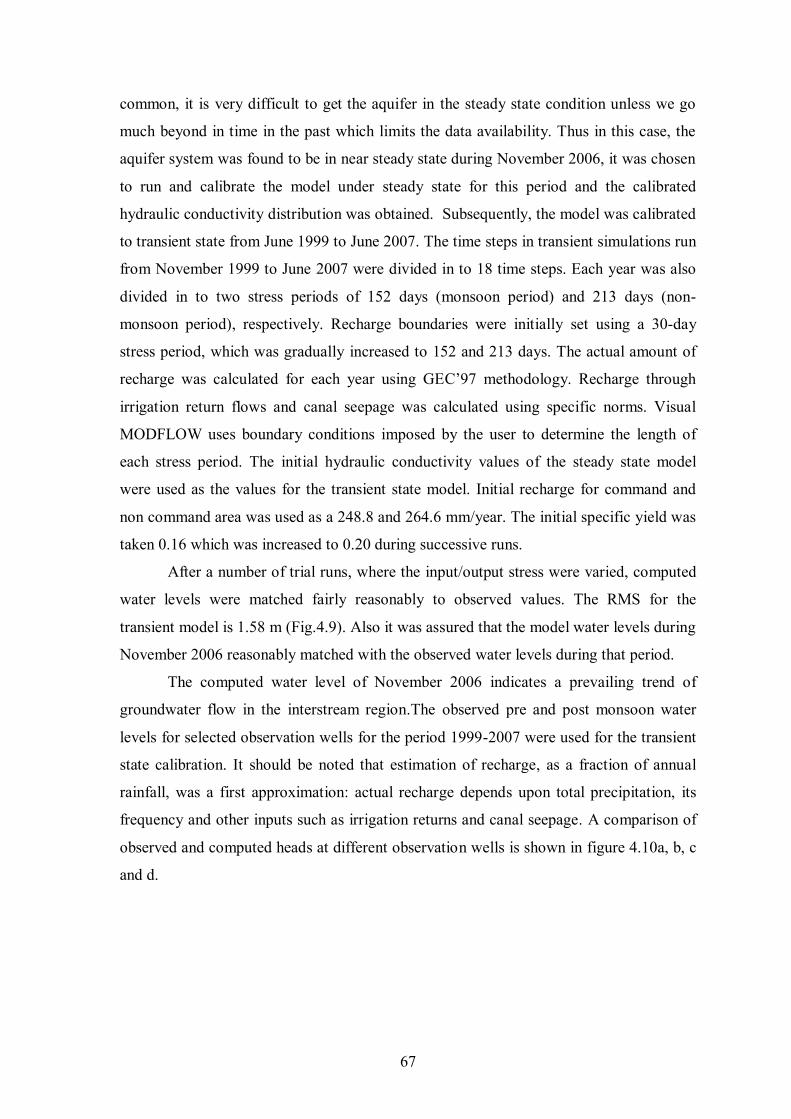
67
common, it is very difficult to get the aquifer in the steady state condition unless we go
much beyond in time in the past which limits the data availability. Thus in this case, the
aquifer system was found to be in near steady state during November 2006, it was chosen
to run and calibrate the model under steady state for this period and the calibrated
hydraulic conductivity distribution was obtained. Subsequently, the model was calibrated
to transient state from June 1999 to June 2007. The time steps in transient simulations run
from November 1999 to June 2007 were divided in to 18 time steps. Each year was also
divided in to two stress periods of 152 days (monsoon period) and 213 days (non-
monsoon period), respectively. Recharge boundaries were initially set using a 30-day
stress period, which was gradually increased to 152 and 213 days. The actual amount of
recharge was calculated for each year using GEC’97 methodology. Recharge through
irrigation return flows and canal seepage was calculated using specific norms. Visual
MODFLOW uses boundary conditions imposed by the user to determine the length of
each stress period. The initial hydraulic conductivity values of the steady state model
were used as the values for the transient state model. Initial recharge for command and
non command area was used as a 248.8 and 264.6 mm/year. The initial specific yield was
taken 0.16 which was increased to 0.20 during successive runs.
After a number of trial runs, where the input/output stress were varied, computed
water levels were matched fairly reasonably to observed values. The RMS for the
transient model is 1.58 m (Fig.4.9). Also it was assured that the model water levels during
November 2006 reasonably matched with the observed water levels during that period.
The computed water level of November 2006 indicates a prevailing trend of
groundwater flow in the interstream region.The observed pre and post monsoon water
levels for selected observation wells for the period 1999-2007 were used for the transient
state calibration. It should be noted that estimation of recharge, as a fraction of annual
rainfall, was a first approximation: actual recharge depends upon total precipitation, its
frequency and other inputs such as irrigation returns and canal seepage. A comparison of
observed and computed heads at different observation wells is shown in figure 4.10a, b, c
and d.
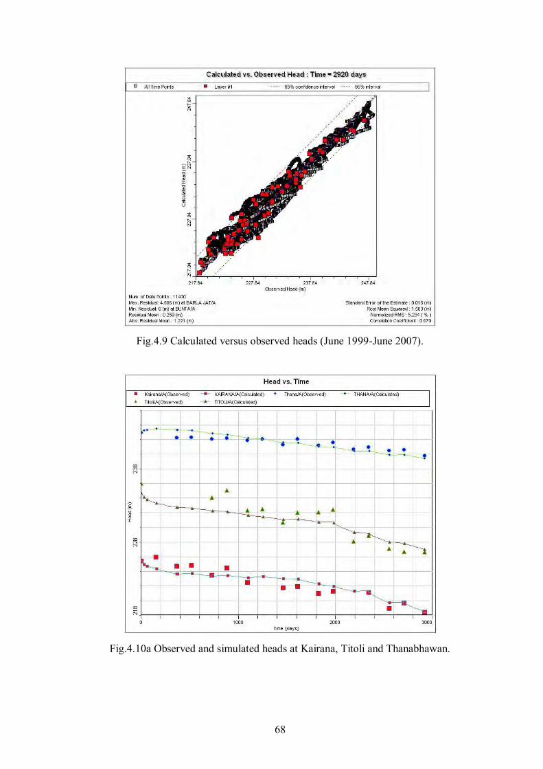
68
Fig.4.9 Calculated versus observed heads (June 1999-June 2007).
Fig.4.10a Observed and simulated heads at Kairana, Titoli and Thanabhawan.
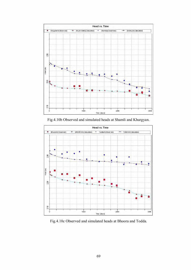
69
Fig.4.10b Observed and simulated heads at Shamli and Khurgyan.
Fig.4.10c Observed and simulated heads at Bhoora and Todda.
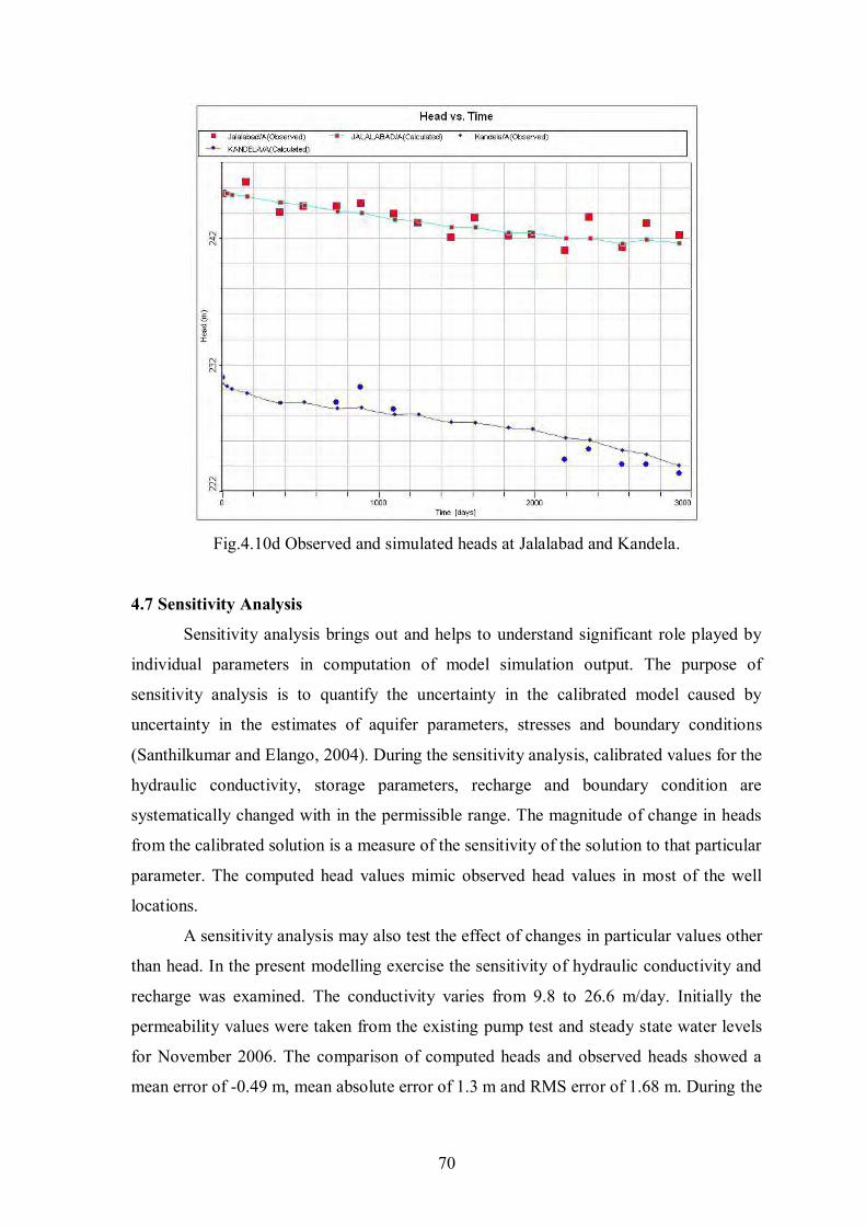
70
Fig.4.10d Observed and simulated heads at Jalalabad and Kandela.
4.7 Sensitivity Analysis
Sensitivity analysis brings out and helps to understand significant role played by
individual parameters in computation of model simulation output. The purpose of
sensitivity analysis is to quantify the uncertainty in the calibrated model caused by
uncertainty in the estimates of aquifer parameters, stresses and boundary conditions
(Santhilkumar and Elango, 2004). During the sensitivity analysis, calibrated values for the
hydraulic conductivity, storage parameters, recharge and boundary condition are
systematically changed with in the permissible range. The magnitude of change in heads
from the calibrated solution is a measure of the sensitivity of the solution to that particular
parameter. The computed head values mimic observed head values in most of the well
locations.
A sensitivity analysis may also test the effect of changes in particular values other
than head. In the present modelling exercise the sensitivity of hydraulic conductivity and
recharge was examined. The conductivity varies from 9.8 to 26.6 m/day. Initially the
permeability values were taken from the existing pump test and steady state water levels
for November 2006. The comparison of computed heads and observed heads showed a
mean error of -0.49 m, mean absolute error of 1.3 m and RMS error of 1.68 m. During the
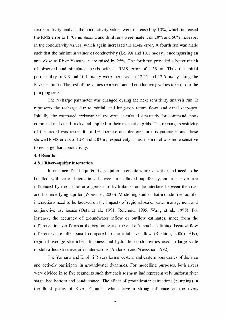
71
first sensitivity analysis the conductivity values were increased by 10%, which increased
the RMS error to 1.703 m. Second and third runs were made with 20% and 50% increases
in the conductivity values, which again increased the RMS error. A fourth run was made
such that the minimum values of conductivity (i.e. 9.8 and 10.1 m/day), encompassing an
area close to River Yamuna, were raised by 25%. The forth run provided a better match
of observed and simulated heads with a RMS error of 1.58 m. Thus the initial
permeability of 9.8 and 10.1 m/day were increased to 12.25 and 12.6 m/day along the
River Yamuna. The rest of the values represent actual conductivity values taken from the
pumping tests.
The recharge parameter was changed during the next sensitivity analysis run. It
represents the recharge due to rainfall and irrigation return flows and canal seepages.
Initially, the estimated recharge values were calculated separately for command, non-
command and canal tracks and applied to their respective grids. The recharge sensitivity
of the model was tested for a 1% increase and decrease in this parameter and these
showed RMS errors of 1.64 and 2.03 m, respectively. Thus, the model was more sensitive
to recharge than conductivity.
4.8 Results
4.8.1 River-aquifer interaction
In an unconfined aquifer river-aquifer interactions are sensitive and need to be
handled with care. Interactions between an alluvial aquifer system and river are
influenced by the spatial arrangement of hydrofacies at the interface between the river
and the underlying aquifer (Woessner, 2000). Modelling studies that include river aquifer
interactions need to be focused on the impacts of regional scale, water management and
conjunctive use issues (Onta et al., 1991; Reichard, 1995; Wang et al., 1995). For
instance, the accuracy of groundwater inflow or outflow estimates, made from the
difference in river flows at the beginning and the end of a reach, is limited because flow
differences are often small compared to the total river flow (Rushton, 2006). Also,
regional average streambed thickness and hydraulic conductivities used in large scale
models affect stream-aquifer interactions (Anderson and Woessner, 1992).
The Yamuna and Krishni Rivers forms western and eastern boundaries of the area
and actively participate in groundwater dynamics. For modelling purposes, both rivers
were divided in to five segments such that each segment had representively uniform river
stage, bed bottom and conductance. The effect of groundwater extractions (pumping) in
the flood plains of River Yamuna, which have a strong influence on the rivers
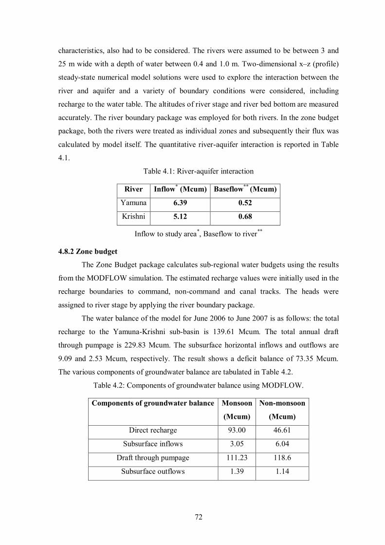
72
characteristics, also had to be considered. The rivers were assumed to be between 3 and
25 m wide with a depth of water between 0.4 and 1.0 m. Two-dimensional x–z (profile)
steady-state numerical model solutions were used to explore the interaction between the
river and aquifer and a variety of boundary conditions were considered, including
recharge to the water table. The altitudes of river stage and river bed bottom are measured
accurately. The river boundary package was employed for both rivers. In the zone budget
package, both the rivers were treated as individual zones and subsequently their flux was
calculated by model itself. The quantitative river-aquifer interaction is reported in Table
4.1.
Table 4.1: River-aquifer interaction
River Inflow* (Mcum) Baseflow** (Mcum)
Yamuna 6.39 0.52
Krishni 5.12 0.68
Inflow to study area*, Baseflow to river**
4.8.2 Zone budget
The Zone Budget package calculates sub-regional water budgets using the results
from the MODFLOW simulation. The estimated recharge values were initially used in the
recharge boundaries to command, non-command and canal tracks. The heads were
assigned to river stage by applying the river boundary package.
The water balance of the model for June 2006 to June 2007 is as follows: the total
recharge to the Yamuna-Krishni sub-basin is 139.61 Mcum. The total annual draft
through pumpage is 229.83 Mcum. The subsurface horizontal inflows and outflows are
9.09 and 2.53 Mcum, respectively. The result shows a deficit balance of 73.35 Mcum.
The various components of groundwater balance are tabulated in Table 4.2.
Table 4.2: Components of groundwater balance using MODFLOW.
Components of groundwater balance Monsoon
(Mcum)
Non-monsoon
(Mcum)
Direct recharge 93.00 46.61
Subsurface inflows 3.05 6.04
Draft through pumpage 111.23 118.6
Subsurface outflows 1.39 1.14
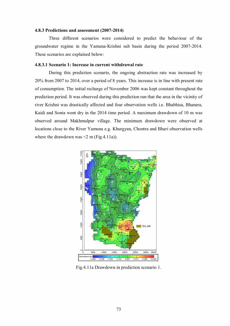
73
4.8.3 Predictions and assessment (2007-2014)
Three different scenarios were considered to predict the behaviour of the
groundwater regime in the Yamuna-Krishni sub basin during the period 2007-2014.
These scenarios are explained below:
4.8.3.1 Scenario 1: Increase in current withdrawal rate
During this prediction scenario, the ongoing abstraction rate was increased by
20% from 2007 to 2014, over a period of 8 years. This increase is in line with present rate
of consumption. The initial recharge of November 2006 was kept constant throughout the
prediction period. It was observed during this prediction run that the area in the vicinity of
river Krishni was drastically affected and four observation wells i.e. Bhabhisa, Bhanera,
Kaidi and Sonta went dry in the 2014 time period. A maximum drawdown of 10 m was
observed around Makhmulpur village. The minimum drawdown were observed at
locations close to the River Yamuna e.g. Khurgyan, Chontra and Bhari observation wells
where the drawdown was <2 m (Fig.4.11a)).
Fig.4.11a Drawdown in prediction scenario 1.
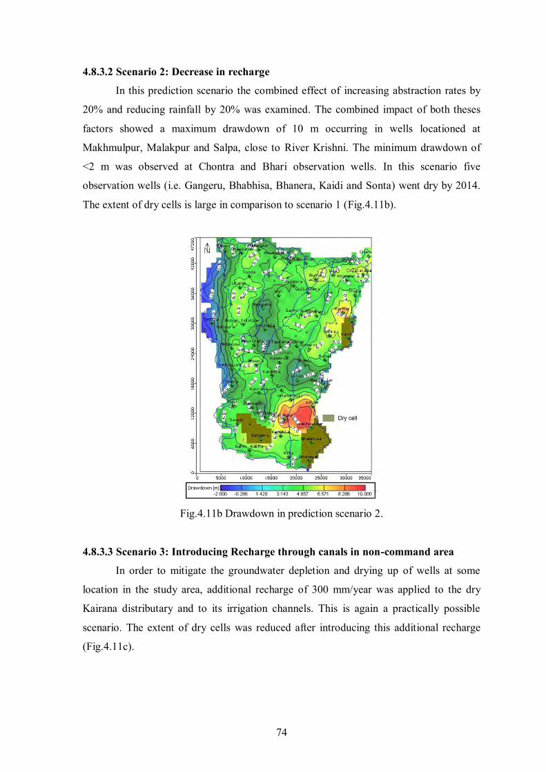
74
4.8.3.2 Scenario 2: Decrease in recharge
In this prediction scenario the combined effect of increasing abstraction rates by
20% and reducing rainfall by 20% was examined. The combined impact of both theses
factors showed a maximum drawdown of 10 m occurring in wells locationed at
Makhmulpur, Malakpur and Salpa, close to River Krishni. The minimum drawdown of
<2 m was observed at Chontra and Bhari observation wells. In this scenario five
observation wells (i.e. Gangeru, Bhabhisa, Bhanera, Kaidi and Sonta) went dry by 2014.
The extent of dry cells is large in comparison to scenario 1 (Fig.4.11b).
Fig.4.11b Drawdown in prediction scenario 2.
4.8.3.3 Scenario 3: Introducing Recharge through canals in non-command area
In order to mitigate the groundwater depletion and drying up of wells at some
location in the study area, additional recharge of 300 mm/year was applied to the dry
Kairana distributary and to its irrigation channels. This is again a practically possible
scenario. The extent of dry cells was reduced after introducing this additional recharge
(Fig.4.11c).
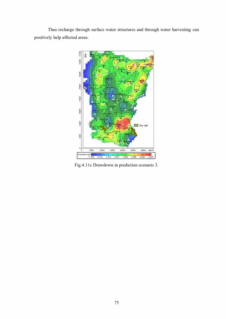
75
Thus recharge through surface water structures and through water harvesting can
positively help affected areas.
Fig.4.11c Drawdown in prediction scenario 3.
76
5 - GROUNDWATER VULNERABILITY ASSESSMENT
5.1 Introduction
In the past few decades groundwater contamination has become one of the most
serious problems in the world. Once polluted, remediation of aquifers would be very
difficult, and even sometimes it becomes impossible to restore to its original quality
(Qinghai et al., 2007). Alluvial areas like Central Ganga Plain (CGP), where groundwater
is easily accessible from shallow water table aquifers, need proper protection of
groundwater regime from contamination. The groundwater utilization has increased
manifold due to advancement in agrarian sector together with rapid industrialization. The
groundwater abstraction from shallow aquifers is continuously on the rise which could be
related to multifarious problems, like overexploitation, and quality deterioration, thus
posing threats to the sustainability of this precious resource.
Vulnerability assessment of groundwater, as used in many methods, is not a
characteristic that can be directly measured in the field. It is an idea based on the
fundamental concept “that some land areas are more vulnerable to groundwater
contamination than others” (Vrba and Zaporozec., 1994).
Vulnerability mapping involves combining several thematic maps of selected
physical resource factors into a groundwater vulnerability map that identifies different
areas of the sensitivity of groundwater to natural and human impacts. The original
concept of groundwater vulnerability was based on assumption that the physical
environment may provide some degree of protection to groundwater with regard to
contaminants entering the sub-surface. The earth materials may act as natural filter to
screen out some contaminants. Water infiltrating at the land surface may be contaminated
but is naturally purified to some degree as it percolates through the soil and other fine
grained material in the unsaturated zone.
In recent years, groundwater vulnerability assessment has become very useful tool
for planning and decision making of groundwater protection (Vias et al., 2005). However,
it is important to note that vulnerability maps are not panacea. They are simply just one of
the many tools available for groundwater protection programmes. The main value of
vulnerability maps is that they can be used as an effective preliminary tool for the
planning, policy and operational levels of the decision making process concerning
groundwater management and protection (Vrba and Zeporozec, 1994).
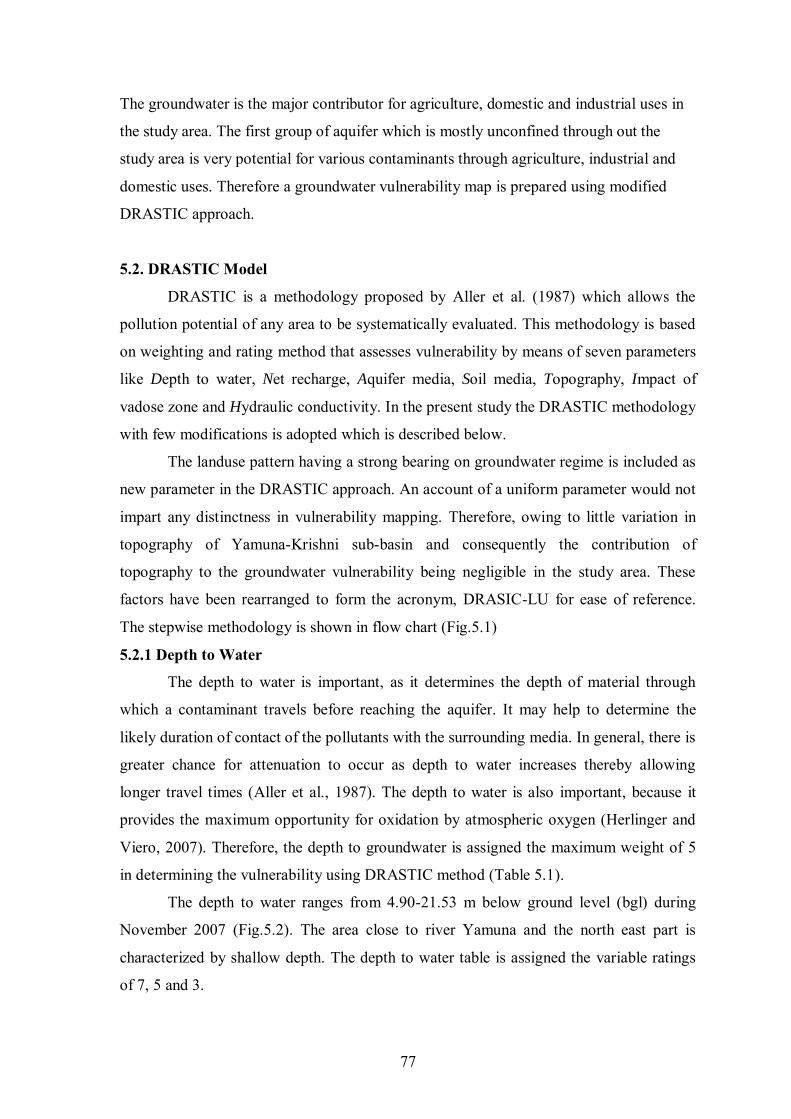
77
The groundwater is the major contributor for agriculture, domestic and industrial uses in
the study area. The first group of aquifer which is mostly unconfined through out the
study area is very potential for various contaminants through agriculture, industrial and
domestic uses. Therefore a groundwater vulnerability map is prepared using modified
DRASTIC approach.
5.2. DRASTIC Model
DRASTIC is a methodology proposed by Aller et al. (1987) which allows the
pollution potential of any area to be systematically evaluated. This methodology is based
on weighting and rating method that assesses vulnerability by means of seven parameters
like Depth to water, Net recharge, Aquifer media, Soil media, Topography, Impact of
vadose zone and Hydraulic conductivity. In the present study the DRASTIC methodology
with few modifications is adopted which is described below.
The landuse pattern having a strong bearing on groundwater regime is included as
new parameter in the DRASTIC approach. An account of a uniform parameter would not
impart any distinctness in vulnerability mapping. Therefore, owing to little variation in
topography of Yamuna-Krishni sub-basin and consequently the contribution of
topography to the groundwater vulnerability being negligible in the study area. These
factors have been rearranged to form the acronym, DRASIC-LU for ease of reference.
The stepwise methodology is shown in flow chart (Fig.5.1)
5.2.1 Depth to Water
The depth to water is important, as it determines the depth of material through
which a contaminant travels before reaching the aquifer. It may help to determine the
likely duration of contact of the pollutants with the surrounding media. In general, there is
greater chance for attenuation to occur as depth to water increases thereby allowing
longer travel times (Aller et al., 1987). The depth to water is also important, because it
provides the maximum opportunity for oxidation by atmospheric oxygen (Herlinger and
Viero, 2007). Therefore, the depth to groundwater is assigned the maximum weight of 5
in determining the vulnerability using DRASTIC method (Table 5.1).
The depth to water ranges from 4.90-21.53 m below ground level (bgl) during
November 2007 (Fig.5.2). The area close to river Yamuna and the north east part is
characterized by shallow depth. The depth to water table is assigned the variable ratings
of 7, 5 and 3.
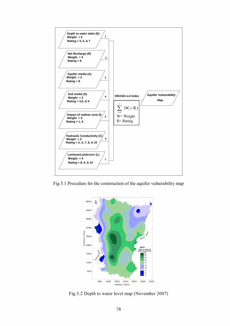
78
Depth to water table (D)
Net Recharge (R)
Aquifer media (A)
Soil media (S)
Impact of vadose zone (I)
Hydraulic Conductivity (C)
Landuse/Landcover (L)
Weight = 5
Rating = 3, 5, & 7
Weight = 4
Weight = 3
Weight = 2
Weight = 5
Weight = 3
Rating = 9
Rating = 8
Rating = 3,5, & 6
Rating = 1, 6
Rating = 2, 4, 7, 8, & 10
Weight = 5
Rating = 8, 9, & 10
DRASIC-LU Index Aquifer Vulnerability
Map
1
2
3
4
5
6
7
Fig.5.1 Procedure for the construction of the aquifer vulnerability map
Fig.5.2 Depth to water level map (November 2007)
)(7
1ii
i
RW
W= Weight R= Rating
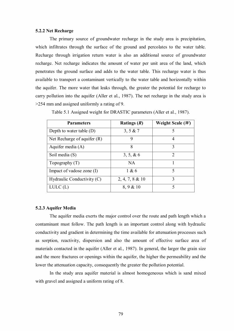
79
5.2.2 Net Recharge
The primary source of groundwater recharge in the study area is precipitation,
which infiltrates through the surface of the ground and percolates to the water table.
Recharge through irrigation return water is also an additional source of groundwater
recharge. Net recharge indicates the amount of water per unit area of the land, which
penetrates the ground surface and adds to the water table. This recharge water is thus
available to transport a contaminant vertically to the water table and horizontally within
the aquifer. The more water that leaks through, the greater the potential for recharge to
carry pollution into the aquifer (Aller et al., 1987). The net recharge in the study area is
>254 mm and assigned uniformly a rating of 9.
Table 5.1 Assigned weight for DRASTIC parameters (Aller et al., 1987).
Parameters Ratings (R) Weight Scale (W)
Depth to water table (D) 3, 5 & 7 5
Net Recharge of aquifer (R) 9 4
Aquifer media (A) 8 3
Soil media (S) 3, 5, & 6 2
Topography (T) NA 1
Impact of vadose zone (I) 1 & 6 5
Hydraulic Conductivity (C) 2, 4, 7, 8 & 10 3
LULC (L) 8, 9 & 10 5
5.2.3 Aquifer Media
The aquifer media exerts the major control over the route and path length which a
contaminant must follow. The path length is an important control along with hydraulic
conductivity and gradient in determining the time available for attenuation processes such
as sorption, reactivity, dispersion and also the amount of effective surface area of
materials contacted in the aquifer (Aller et al., 1987). In general, the larger the grain size
and the more fractures or openings within the aquifer, the higher the permeability and the
lower the attenuation capacity, consequently the greater the pollution potential.
In the study area aquifer material is almost homogeneous which is sand mixed
with gravel and assigned a uniform rating of 8.
80
5.2.4 Soil Media
Soil is commonly considered the upper weathered zone of the earth which
averages 1.8 m or less. It has a significant impact on the amount of recharge water which
can infiltrate into the ground and hence, influence the ability of a contaminant to move
vertically into the vadose zone. In general, the pollution potential of a soil is largely
affected by the type of clay present and the grain size of the soil. The study area is
characterized by three types of soil viz. loam, clay loam and sandy loam (Fig. 5.3), which
correspond to ratings of 5, 3 and 6 respectively.
Fig.5.3 Soil map of the study area
5.2.5 Impact of Vadose Zone
The vadose zone media determines the attenuation characteristics of the material
below the typical soil horizon and above the water table. The media also controls the path
length and routing, thus affecting the time available for attenuation and the quality of
material encountered. The materials forming the vadose zone in the study area are clay,
silt and fine sand which are corresponding to the ratings 1 and 6. The assigned weight for
vadose zone is 5.
It was observed that the characterization of vadose zone is significant due to
alternation between clay and fine sand, both possessing distinct hydrological character.
The initial ratings of 1 and 6 for clay and fine sand do not sufficiently incorporate their
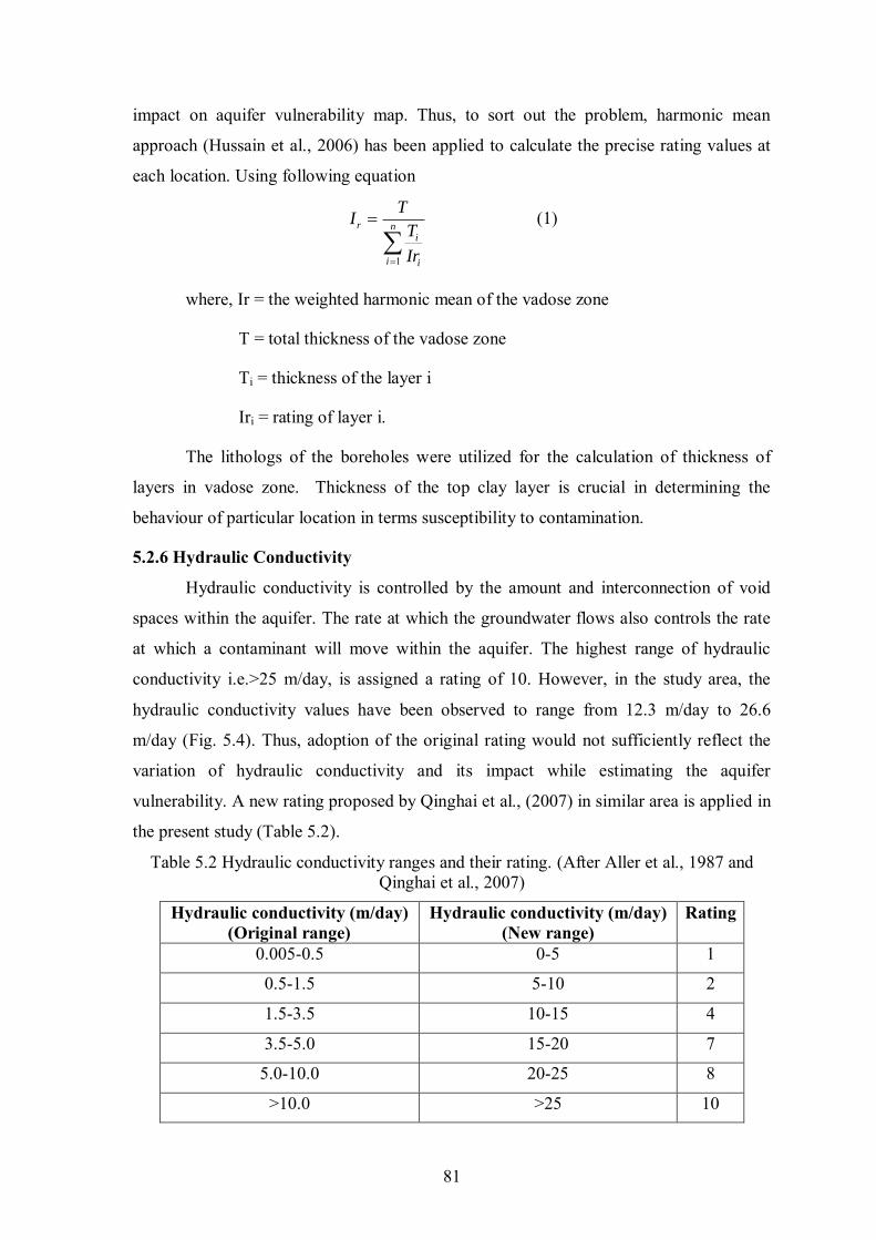
81
impact on aquifer vulnerability map. Thus, to sort out the problem, harmonic mean
approach (Hussain et al., 2006) has been applied to calculate the precise rating values at
each location. Using following equation
n
i i
i
r
Ir
T
TI
1
(1)
where, Ir = the weighted harmonic mean of the vadose zone
T = total thickness of the vadose zone
Ti = thickness of the layer i
Iri = rating of layer i.
The lithologs of the boreholes were utilized for the calculation of thickness of
layers in vadose zone. Thickness of the top clay layer is crucial in determining the
behaviour of particular location in terms susceptibility to contamination.
5.2.6 Hydraulic Conductivity
Hydraulic conductivity is controlled by the amount and interconnection of void
spaces within the aquifer. The rate at which the groundwater flows also controls the rate
at which a contaminant will move within the aquifer. The highest range of hydraulic
conductivity i.e.>25 m/day, is assigned a rating of 10. However, in the study area, the
hydraulic conductivity values have been observed to range from 12.3 m/day to 26.6
m/day (Fig. 5.4). Thus, adoption of the original rating would not sufficiently reflect the
variation of hydraulic conductivity and its impact while estimating the aquifer
vulnerability. A new rating proposed by Qinghai et al., (2007) in similar area is applied in
the present study (Table 5.2).
Table 5.2 Hydraulic conductivity ranges and their rating. (After Aller et al., 1987 and Qinghai et al., 2007)
Hydraulic conductivity (m/day) (Original range)
Hydraulic conductivity (m/day) (New range)
Rating
0.005-0.5 0-5 1
0.5-1.5 5-10 2
1.5-3.5 10-15 4
3.5-5.0 15-20 7
5.0-10.0 20-25 8
>10.0 >25 10
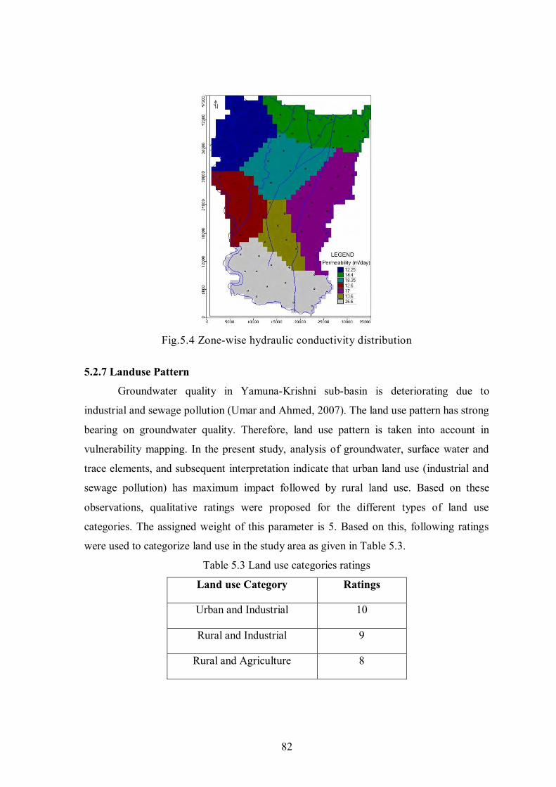
82
Fig.5.4 Zone-wise hydraulic conductivity distribution
5.2.7 Landuse Pattern
Groundwater quality in Yamuna-Krishni sub-basin is deteriorating due to
industrial and sewage pollution (Umar and Ahmed, 2007). The land use pattern has strong
bearing on groundwater quality. Therefore, land use pattern is taken into account in
vulnerability mapping. In the present study, analysis of groundwater, surface water and
trace elements, and subsequent interpretation indicate that urban land use (industrial and
sewage pollution) has maximum impact followed by rural land use. Based on these
observations, qualitative ratings were proposed for the different types of land use
categories. The assigned weight of this parameter is 5. Based on this, following ratings
were used to categorize land use in the study area as given in Table 5.3.
Table 5.3 Land use categories ratings
Land use Category Ratings
Urban and Industrial 10
Rural and Industrial 9
Rural and Agriculture 8
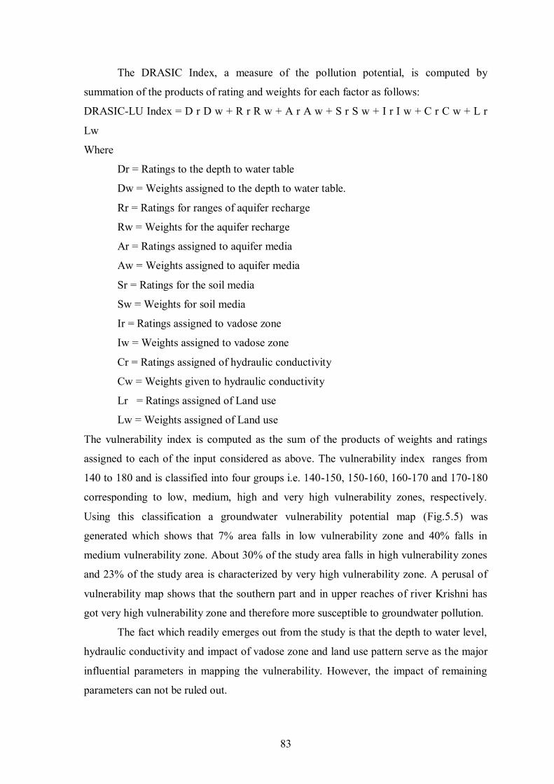
83
The DRASIC Index, a measure of the pollution potential, is computed by
summation of the products of rating and weights for each factor as follows:
DRASIC-LU Index = D r D w + R r R w + A r A w + S r S w + I r I w + C r C w + L r
Lw
Where
Dr = Ratings to the depth to water table
Dw = Weights assigned to the depth to water table.
Rr = Ratings for ranges of aquifer recharge
Rw = Weights for the aquifer recharge
Ar = Ratings assigned to aquifer media
Aw = Weights assigned to aquifer media
Sr = Ratings for the soil media
Sw = Weights for soil media
Ir = Ratings assigned to vadose zone
Iw = Weights assigned to vadose zone
Cr = Ratings assigned of hydraulic conductivity
Cw = Weights given to hydraulic conductivity
Lr = Ratings assigned of Land use
Lw = Weights assigned of Land use
The vulnerability index is computed as the sum of the products of weights and ratings
assigned to each of the input considered as above. The vulnerability index ranges from
140 to 180 and is classified into four groups i.e. 140-150, 150-160, 160-170 and 170-180
corresponding to low, medium, high and very high vulnerability zones, respectively.
Using this classification a groundwater vulnerability potential map (Fig.5.5) was
generated which shows that 7% area falls in low vulnerability zone and 40% falls in
medium vulnerability zone. About 30% of the study area falls in high vulnerability zones
and 23% of the study area is characterized by very high vulnerability zone. A perusal of
vulnerability map shows that the southern part and in upper reaches of river Krishni has
got very high vulnerability zone and therefore more susceptible to groundwater pollution.
The fact which readily emerges out from the study is that the depth to water level,
hydraulic conductivity and impact of vadose zone and land use pattern serve as the major
influential parameters in mapping the vulnerability. However, the impact of remaining
parameters can not be ruled out.
84
Fig. 5.5 Aquifer vulnerability map of the Yamuna-Krishni sub-basin.
The southern part is characterized by very high vulnerability index which is
attributed to high values of hydraulic conductivity and aquifer thickness. The few patches
in the vicinity of the river Yamuna constituting the Yamuna Flood Plain (YFP) are
characterized by high vulnerability index, which in turn is attributed to shallow water
level (5-7 m bgl) and thin vadose zone.
85
The area just east of Yamuna flood plain is the zone of medium vulnerability. The
moderate risk to groundwater contamination is mainly attributed to the presence of thick
vadose zone containing clay layers and comparatively of low hydraulic conductivity,
particularly in the northern part. The presence or absence of clay layer affects the
pollution attenuation capacity. The clay is abundant in the northern part and gradually
decreases due south and serves as the most variable parameter with ratings of 1 and 6.
The groundwater vulnerability potential map shows that bulk of the area is
covered by high to very high vulnerable zone followed by medium and low vulnerable
zones. Ironically, all major townships like Shamli, Kairana and Kandhala are located in
high to very high vulnerability zones. The vulnerability map thus generated helps in
identifying areas which are more likely to be susceptible to groundwater contamination
relative to one another.
86
6 - HYDROGEOCHEMISTRY
6.1 Introduction
Water is frequently referred as universal solvent, because it has the ability to
dissolve at least some amount of all substance that comes in contact. Rainfall and snow
melt percolating through the soil zone and unsaturated material chemically reacts with the
gases, minerals and organic compounds that occur naturally within the subsurface. These
reactions continue below the water table as the water flows through the aquifer. The result
is that the characteristics and composition of the water evolve as it flows through the
ground in response to the types of solids and gas phases that the solution encounters and
the geochemical reactions that occur between these phases (Deutsch, 1997). Therefore,
each groundwater system has its own characteristic chemical signature produced as a
result of chemical alteration of the meteoric water recharging the system (Drever, 1982).
The study of a relatively large group of samples from a given area offers clues to
various possible trends of chemical alteration which the meteoric water undergoes before
acquiring distinct chemical characteristics and attaining a chemical steady state in the
aquifer. These identified trends in turn may be related to natural and anthropogenic
causative factors (Umar and Absar, 2003). With this simple objective in sight systematic
sampling was carried out in the study area from the point of view of understanding
various possible sources of dissolved ions and to assess the seasonal variation in
groundwater quality with respect to drinking and irrigational uses.
6.2 Methodology
6.2.1 Sample Collection
Due to probable seasonal variation in the water quality. One forty four
groundwater samples were collected for physico-chemical analysis in four successive
season’s viz. post-monsoon and pre-monsoon period corresponding November 2005, June
2006, November 2006 and June 2007 respectively (Fig. 6.1). In November 2005 and June
2007, seven and 9 surface water samples were also collected (Appendix VIIIA, B) from
river Yamuna and Krishni respectively (Plate-7a and 7b). In addition four samples were
also collected from Nala/Drain (Appendix VIIIC) for major ion analysis (Plate-8a and
8b). The water samples were collected and stored in 1 litre capacity clean plastic bottles.
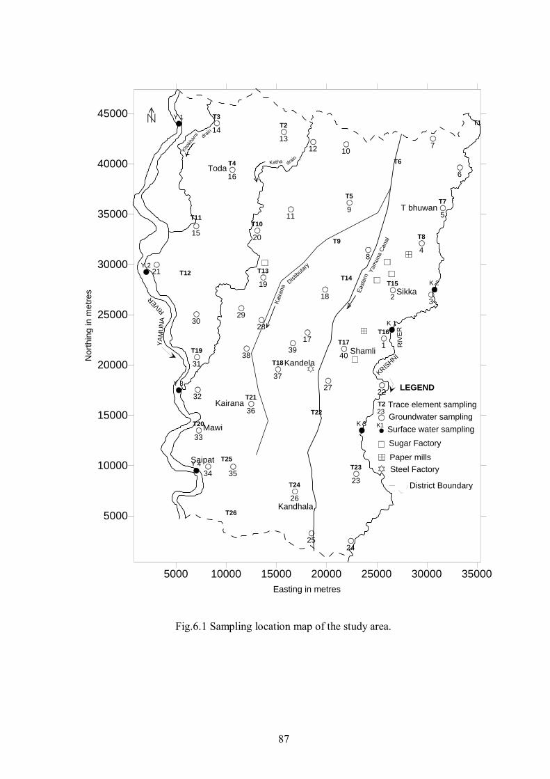
87
5000 10000 15000 20000 25000 30000 35000
Easting in metres
5000
10000
15000
20000
25000
30000
35000
40000
45000
Nort
hin
g in
metr
es
1
23
4
5
6
7
8
9
10
11
12
1314
15
16
17
18
19
20
21
22
23
2425
26
27
28
2930
31
32
33
34 35
36
37
3839
40
K 1
K 2
K 3
Y 1
Y 2
Y 3
Y 4
T1T2
T3
T4
T5
T6
T7
T8T9
T10T11
T12 T13T14
T15
T16
T17
T18
T19
T20
T21
T22
T23
T24
T25
T26
LEGEND
Kairana
Shamli
T bhuwan
Toda
Kandhala
YA
MU
NA
RIV
ER
District Boundary
KRIS
HNI
RIV
ER
East
ern
Yam
una C
anal
Kairana
Distib
utar
y
Katha drain
Kho
khar
ni drain
Groundwater sampling
Surface water sampling
Sugar Factory
Paper millsSaipat
Mawi
Sikka
23
K1
Steel Factory
T2 Trace element sampling
Kandela
Fig.6.1 Sampling location map of the study area.
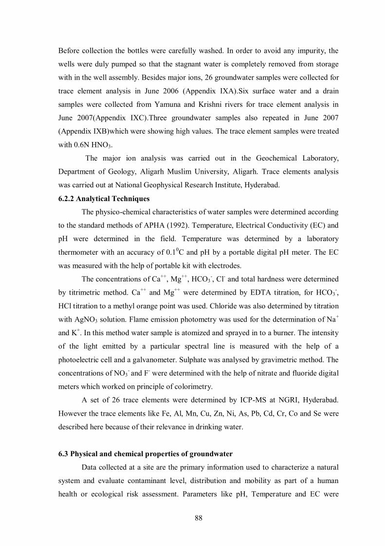
88
Before collection the bottles were carefully washed. In order to avoid any impurity, the
wells were duly pumped so that the stagnant water is completely removed from storage
with in the well assembly. Besides major ions, 26 groundwater samples were collected for
trace element analysis in June 2006 (Appendix IXA).Six surface water and a drain
samples were collected from Yamuna and Krishni rivers for trace element analysis in
June 2007(Appendix IXC).Three groundwater samples also repeated in June 2007
(Appendix IXB)which were showing high values. The trace element samples were treated
with 0.6N HNO3.
The major ion analysis was carried out in the Geochemical Laboratory,
Department of Geology, Aligarh Muslim University, Aligarh. Trace elements analysis
was carried out at National Geophysical Research Institute, Hyderabad.
6.2.2 Analytical Techniques
The physico-chemical characteristics of water samples were determined according
to the standard methods of APHA (1992). Temperature, Electrical Conductivity (EC) and
pH were determined in the field. Temperature was determined by a laboratory
thermometer with an accuracy of 0.10C and pH by a portable digital pH meter. The EC
was measured with the help of portable kit with electrodes.
The concentrations of Ca++, Mg++, HCO3-, Cl- and total hardness were determined
by titrimetric method. Ca++ and Mg++ were determined by EDTA titration, for HCO3-,
HCl titration to a methyl orange point was used. Chloride was also determined by titration
with AgNO3 solution. Flame emission photometry was used for the determination of Na+
and K+. In this method water sample is atomized and sprayed in to a burner. The intensity
of the light emitted by a particular spectral line is measured with the help of a
photoelectric cell and a galvanometer. Sulphate was analysed by gravimetric method. The
concentrations of NO3- and F- were determined with the help of nitrate and fluoride digital
meters which worked on principle of colorimetry.
A set of 26 trace elements were determined by ICP-MS at NGRI, Hyderabad.
However the trace elements like Fe, Al, Mn, Cu, Zn, Ni, As, Pb, Cd, Cr, Co and Se were
described here because of their relevance in drinking water.
6.3 Physical and chemical properties of groundwater
Data collected at a site are the primary information used to characterize a natural
system and evaluate contaminant level, distribution and mobility as part of a human
health or ecological risk assessment. Parameters like pH, Temperature and EC were
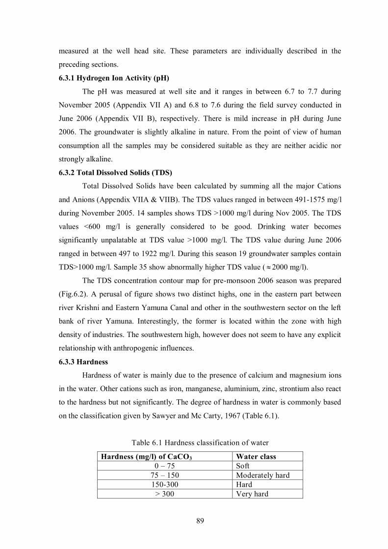
89
measured at the well head site. These parameters are individually described in the
preceding sections.
6.3.1 Hydrogen Ion Activity (pH)
The pH was measured at well site and it ranges in between 6.7 to 7.7 during
November 2005 (Appendix VII A) and 6.8 to 7.6 during the field survey conducted in
June 2006 (Appendix VII B), respectively. There is mild increase in pH during June
2006. The groundwater is slightly alkaline in nature. From the point of view of human
consumption all the samples may be considered suitable as they are neither acidic nor
strongly alkaline.
6.3.2 Total Dissolved Solids (TDS)
Total Dissolved Solids have been calculated by summing all the major Cations
and Anions (Appendix VIIA & VIIB). The TDS values ranged in between 491-1575 mg/l
during November 2005. 14 samples shows TDS >1000 mg/l during Nov 2005. The TDS
values <600 mg/l is generally considered to be good. Drinking water becomes
significantly unpalatable at TDS value >1000 mg/l. The TDS value during June 2006
ranged in between 497 to 1922 mg/l. During this season 19 groundwater samples contain
TDS>1000 mg/l. Sample 35 show abnormally higher TDS value ( 2000 mg/l).
The TDS concentration contour map for pre-monsoon 2006 season was prepared
(Fig.6.2). A perusal of figure shows two distinct highs, one in the eastern part between
river Krishni and Eastern Yamuna Canal and other in the southwestern sector on the left
bank of river Yamuna. Interestingly, the former is located within the zone with high
density of industries. The southwestern high, however does not seem to have any explicit
relationship with anthropogenic influences.
6.3.3 Hardness
Hardness of water is mainly due to the presence of calcium and magnesium ions
in the water. Other cations such as iron, manganese, aluminium, zinc, strontium also react
to the hardness but not significantly. The degree of hardness in water is commonly based
on the classification given by Sawyer and Mc Carty, 1967 (Table 6.1).
Table 6.1 Hardness classification of water
Hardness (mg/l) of CaCO3 Water class 0 – 75 Soft
75 – 150 Moderately hard 150-300 Hard
> 300 Very hard
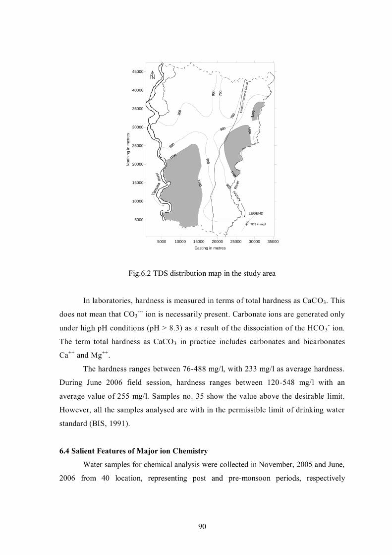
90
5000 10000 15000 20000 25000 30000 35000
Easting in metres
5000
10000
15000
20000
25000
30000
35000
40000
45000
Nort
hin
g in m
etr
es
Kris
hniR
iver
Riv
er
Easte
rn Y
am
una C
anal
LEGEND
900
TDS in mg/l
1100
Fig.6.2 TDS distribution map in the study area
In laboratories, hardness is measured in terms of total hardness as CaCO3. This
does not mean that CO3--- ion is necessarily present. Carbonate ions are generated only
under high pH conditions (pH > 8.3) as a result of the dissociation of the HCO3- ion.
The term total hardness as CaCO3 in practice includes carbonates and bicarbonates
Ca++ and Mg++.
The hardness ranges between 76-488 mg/l, with 233 mg/l as average hardness.
During June 2006 field session, hardness ranges between 120-548 mg/l with an
average value of 255 mg/l. Samples no. 35 show the value above the desirable limit.
However, all the samples analysed are with in the permissible limit of drinking water
standard (BIS, 1991).
6.4 Salient Features of Major ion Chemistry
Water samples for chemical analysis were collected in November, 2005 and June,
2006 from 40 location, representing post and pre-monsoon periods, respectively
91
(Appendix VIIA, VIIB). The salient features of the groundwater chemistry are presented
below.
1. The area has got high total dissolved solids (TDS) values, which range in between
491 to 1575 mg/l with an average value of 922 mg/l during November 2005.
2. Most of the samples have TDS values higher than the desirable limit of 500 mg/l.
The TDS concentration during June 2006 ranges between 497 and 1922 mg/l
averaging 1028 mg/l.
3. The EC values range in between 200 and 800 µmhos/cm and 200 and 1500
µmhos/cm during November 2005 and June 2006, respectively.
4. Major anions show a wide range of variations.
4SO content vary from 42 to 337
mg/l in November 2005 and 49 to 480 mg/l during June 2006. The Cl has
concentration ranges of 11 to 284 and 1 to 346 mg/l and
3HCO ranges between
195 to 780 mg/l and 234 to 715 mg/l during November 2005 and June 2006,
respectively.
5. The
3NO and fluoride analysis were carried out for June 2006 sample and there
concentration ranges between 13 to 150 mg/l and 0.3 to 2.3 mg/l, respectively.
6. In few samples the concentration of
3NO and F- is more than highest desirable
limit. A maximum value of 150 mg/l of
3NO is recorded in sample 2 representing
Sikka village. This value exceeds the permissible limit of drinking water standard
(BIS, 1991).
7. In six samples the fluoride concentration exceeds the maximum permissible limit
of 1.5 mg/l.
8. Alkali ions also show very large variations. Na+ varies from 73 to 384 mg/l in
November 2005 and 42 to 366 mg/l in June 2006. The K+ concentration ranges
between 0 to 116 and 0 to 67 mg/l during November 2005 and June 2006,
respectively.
9. Ca+ and Mg+ comparatively show restricted range of concentration. Ca+
concentration ranges between 6 to 32 mg/l during November 2005 and 5 to 64
mg/l during June 2006. Mg+ content varies from 9 to 110 and 21 to 121 mg/l
during November 2005 and June 2006 respectively.
92
10. Alkalis are the dominant cationic species when compared to Ca+ and Mg+. This
statement hold good for both season’s analysis i.e. pre monsoon and post
monsoon.
11. The HCO3- is the most dominating anionic species in the groundwaters of the
study area. In half of the samples the concentration of SO4- together with Cl-
equals to the HCO3-.
12. The samples were also analysed for their suitability for irrigation purposes using
SAR versus EC diagram (Richards, 1954). The samples, with few exceptions, fall
in good to excellent class.
6.5 Hydrochemical characteristic of Groundwater
A number of x-y plots were prepared for deciphering various chemical alteration
trends of groundwaters and identifying the processes involved in the acquisition of
distinct chemical characteristics.
Alkalis are distinctly far more abundant than Ca++ and Mg++ in both the sets of
samples (Fig.6.3). The HCO3- versus Cl-+SO4
- plot (Fig.6.4) tends to classify the
groundwater in the study area in two groups, i.e. (i) HCO3- > Cl-+SO4
- and (ii) Cl-+SO4-<
HCO3-. Both the plots further indicate that chemical differences between pre and post
monsoon sets of samples are relatively trivial.
The natural tendency between cations and anions to form ionic complexes has
been tested Na++K+ and Cl- (Fig.6.5) and Ca+++Mg++ and HCO3- (Fig.6.6). Without
depicting any noteworthy change in concentration levels recorded in pre- and post
monsoon samples, the majority of the samples plot below 1:1 line on alkali versus Cl- plot
implying surplus Na+ ion over and above those used up in Na-Cl bonding..
Relative abundance of Na+ ions is also implied in molar Cl-/Na+ ratios averaging
around 0.25. Na behaves like a conservative elements as it is not used up in biological
processes and also as an non-conservative elements as it gets fixed in clay mineral
formation by ion exchanges (Subramanian and Sexena, 1983).
The Ca+++Mg++ and HCO3- plot (Fig.6.6) depict a moderately good correlation for
about 40% of all pre and post monsoon samples. Nevertheless, there is considerable
scatter in the plot due to relative preponderance of HCO3-, and this when viewed in the
light of relative abundance of alkali over Ca++ and Mg++ (Fig.6.3) and evidence for
surplus Na+ ions (Fig.6.5) implies that in a considerable number of samples Na-HCO3
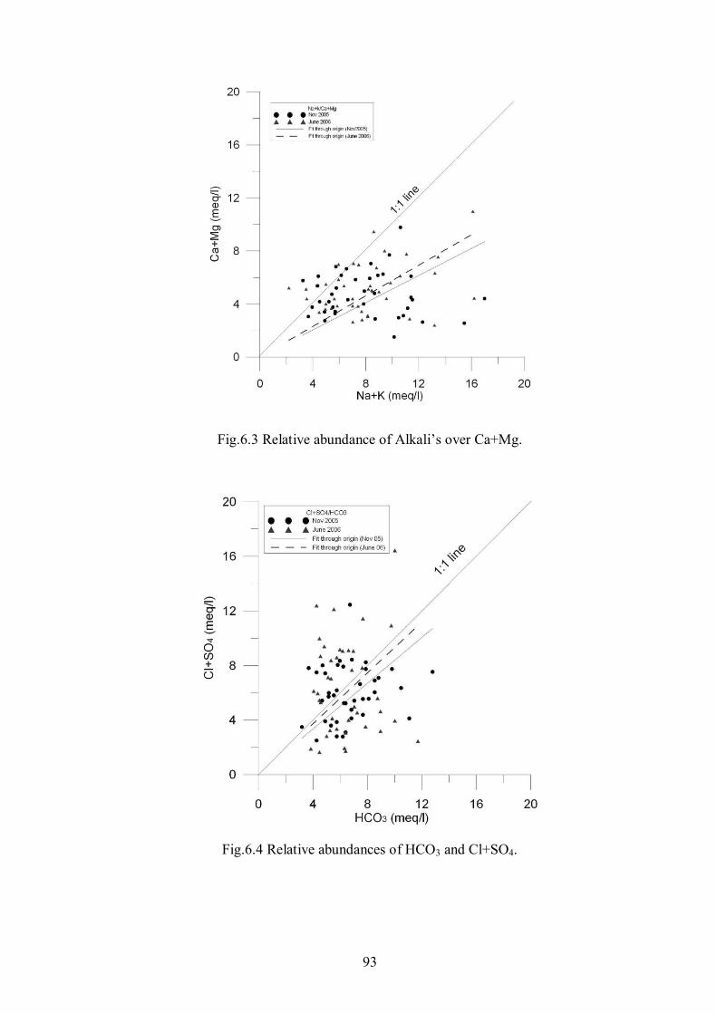
93
Fig.6.3 Relative abundance of Alkali’s over Ca+Mg.
Fig.6.4 Relative abundances of HCO3 and Cl+SO4.
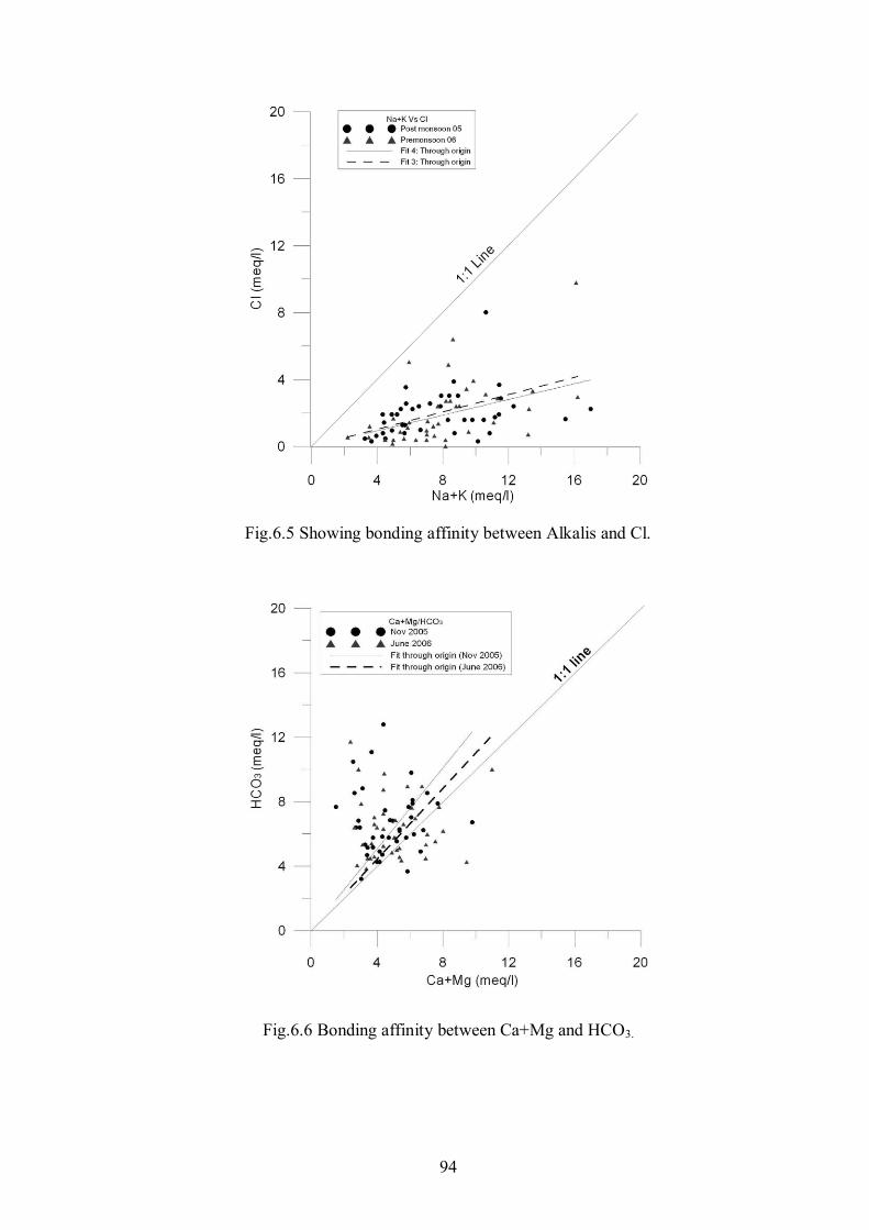
94
Fig.6.5 Showing bonding affinity between Alkalis and Cl.
Fig.6.6 Bonding affinity between Ca+Mg and HCO3.
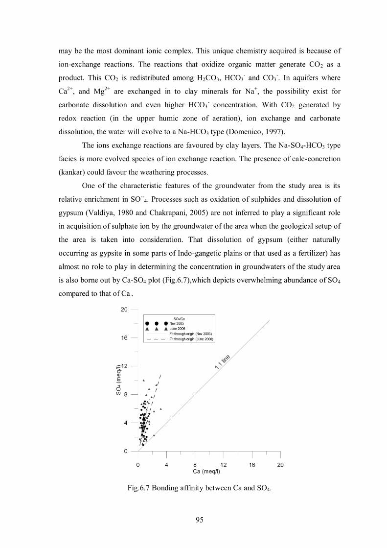
95
may be the most dominant ionic complex. This unique chemistry acquired is because of
ion-exchange reactions. The reactions that oxidize organic matter generate CO2 as a
product. This CO2 is redistributed among H2CO3, HCO3- and CO3
-. In aquifers where
Ca2+, and Mg2+ are exchanged in to clay minerals for Na+, the possibility exist for
carbonate dissolution and even higher HCO3- concentration. With CO2 generated by
redox reaction (in the upper humic zone of aeration), ion exchange and carbonate
dissolution, the water will evolve to a Na-HCO3 type (Domenico, 1997).
The ions exchange reactions are favoured by clay layers. The Na-SO4-HCO3 type
facies is more evolved species of ion exchange reaction. The presence of calc-concretion
(kankar) could favour the weathering processes.
One of the characteristic features of the groundwater from the study area is its
relative enrichment in SO--4. Processes such as oxidation of sulphides and dissolution of
gypsum (Valdiya, 1980 and Chakrapani, 2005) are not inferred to play a significant role
in acquisition of sulphate ion by the groundwater of the area when the geological setup of
the area is taken into consideration. That dissolution of gypsum (either naturally
occurring as gypsite in some parts of Indo-gangetic plains or that used as a fertilizer) has
almost no role to play in determining the concentration in groundwaters of the study area
is also borne out by Ca-SO4 plot (Fig.6.7),which depicts overwhelming abundance of SO4
compared to that of Ca .
Fig.6.7 Bonding affinity between Ca and SO4.
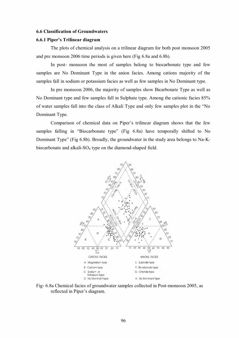
96
6.6 Classification of Groundwaters
6.6.1 Piper’s Trilinear diagram
The plots of chemical analysis on a trilinear diagram for both post monsoon 2005
and pre monsoon 2006 time periods is given here (Fig 6.8a and 6.8b).
In post- monsoon the most of samples belong to biocarbonate type and few
samples are No Dominant Type in the anion facies. Among cations majority of the
samples fall in sodium or potassium facies as well as few samples in No Dominant type.
In pre monsoon 2006, the majority of samples show Bicarbonate Type as well as
No Dominant type and few samples fall in Sulphate type. Among the cationic facies 85%
of water samples fall into the class of Alkali Type and only few samples plot in the “No
Dominant Type.
Comparison of chemical data on Piper’s trilinear diagram shows that the few
samples falling in “Biocarbonate type” (Fig 6.8a) have temporally shifted to No
Dominant Type” (Fig 6.8b). Broadly, the groundwater in the study area belongs to Na-K-
biocarbonate and alkali-SO4 type on the diamond-shaped field.
Fig- 6.8a Chemical facies of groundwater samples collected in Post-monsoon 2005, as reflected in Piper’s diagram.
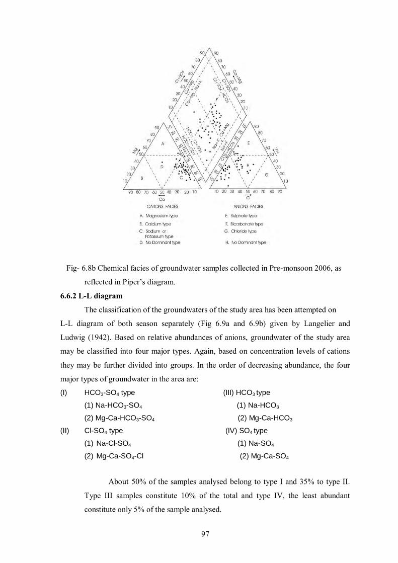
97
Fig- 6.8b Chemical facies of groundwater samples collected in Pre-monsoon 2006, as
reflected in Piper’s diagram.
6.6.2 L-L diagram
The classification of the groundwaters of the study area has been attempted on
L-L diagram of both season separately (Fig 6.9a and 6.9b) given by Langelier and
Ludwig (1942). Based on relative abundances of anions, groundwater of the study area
may be classified into four major types. Again, based on concentration levels of cations
they may be further divided into groups. In the order of decreasing abundance, the four
major types of groundwater in the area are:
(I) HCO3-SO4 type (III) HCO3 type
(1) Na-HCO3-SO4 (1) Na-HCO3
(2) Mg-Ca-HCO3-SO4 (2) Mg-Ca-HCO3
(II) Cl-SO4 type (IV) SO4 type
(1) Na-Cl-SO4 (1) Na-SO4
(2) Mg-Ca-SO4-Cl (2) Mg-Ca-SO4
About 50% of the samples analysed belong to type I and 35% to type II.
Type III samples constitute 10% of the total and type IV, the least abundant
constitute only 5% of the sample analysed.
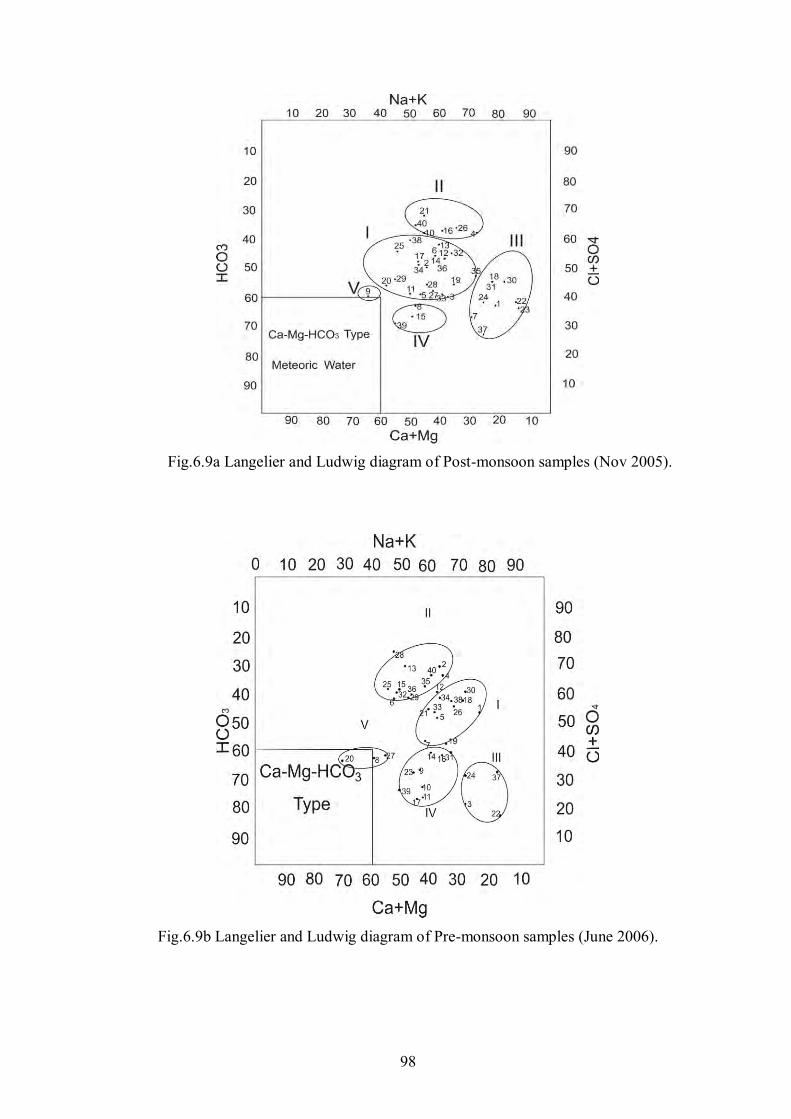
98
Fig.6.9a Langelier and Ludwig diagram of Post-monsoon samples (Nov 2005).
Fig.6.9b Langelier and Ludwig diagram of Pre-monsoon samples (June 2006).
99
6.7 Discussion
The chemical classification attempted earlier based on relative abundances of
anions is further corroborated by L-L diagram of post monsoon samples. Groups I, II and
III in this plot conforms to various sub types of HCO3-SO4 and Cl-SO4 type waters. The
samples, relatively enriched in HCO3 and characterized by Ca+Mg>Na+K, may naturally
be considered less altered and closer to the composition of meteoric water. The
monsoonal effect on groundwater geochemistry as revealed by comparing Fig.6.9a with
that of pre-monsoon samples (Fig.6.9b), however, is not homogeneous. For example,
sample 9 shows relative enrichment of Ca+Mg in the post-monsoon period, whereas
reverse is true for samples 8. Samples 20, 22, 24, 26 and 40, on the other hand show only
trivial or no changes. Thus, the change depicted in the chemistry of groundwater during
pre and post-monsoon period are not explicable in terms of processes, such as,
evaporation, dilution, water rock interaction and variations in residence time. This is also
borne out by the fact that no clear cut alteration trend is depicted in L-L plot of post and
pre monsoon samples (Fig.6.9a and 6.9b). What broadly emerges out is that a set of
samples with composition close to that of meteoric water has basically gained Na and SO4
to results in the various types of groundwater observed in the area. Processes, such as
mixing of two or more types of groundwater or surface water and groundwater, may also
have played a significant role. This phenomenon is depicted to some extent when the
water table map is compared with the map showing distribution of TDS values (Fig.6.2).
TDS values of >1100 mg/l are observed between river Krishni and Eastern Yamuna
Canal, in the eastern part and on the left bank of Yamuna river in the south western part
of the study area. As samples from Krishni river show very high TDS values associated
with high SO4 concentration (Appendix VIII A), it is logical to infer that the western high
TDS zone has been generated as the result of receiving contributions from surface of
industrial waste, particularly effluent from sugar factories, paper mills (Plate-9) and steel
factories. The western high TDS zone evidently has been generated due to east to west
migration of groundwater as highlighted in water table contour maps of the study area.
Except for sample Y4, the other samples collected from Yamuna river have moderate
TDS values of <500 mg/l, consistent with the fact that no industries are located in this
sector. The effluent nature of Yamuna river at sampling site Y4 (Saipat) is evident on the
water table contour map. Sample Y4 is, therefore, the surface manifestation of high TDS
aquifer located on the eastern bank of the river Yamuna. The dynamics of the river
100
aquifer interaction, thus, has played a role in influencing the chemical parameters of
groundwater.
The question that now needs to be answered is as to where from SO4 and Na are
contributed to the system. As far as SO4 is concerned, sulphur finds abundant use is sugar
factories for cleaning sugar solutions. The froth is rejected which on exposure oxidizes to
form SO4, which may find way to shallow aquifers. In addition, SO4 may also be
contributed from community waste and also effluents from industries, such as, paper and
acid manufacturing units which are located in the eastern part of the area. This is
consistent with the fact that samples from Krishni river are highly polluted with TDS of
about 3000 mg/l. Basically, it drains industrial effluents. As far as Na is concerned, this
too is definitely part of the industrial wastes as samples from Krishni river have >200
mg/l of Na, compared to a value of <100 mg/l (except for sample Y4) in Yamuna river.
Very high concentration of K (about 150 mg/l) in Krishni river is really enigmatic and
this is also indicated in groundwater samples 4 and 21 located in the same vicinity. In all
likelihood, K too has origin in community and industrial wastes. Calcium also has high
values in Krishni river and may be related to bleaching powder used in paper industries
and as household disinfectants.
6.8 Trace elements distribution
Trace elements in groundwater are defined as chemical element dissolved in water
in minute quantities, almost always, in concentration less than one milligram of trace
element in one liter of water (USGS, 1993). Although present in small proportion but
their desirable intake is necessary for proper functioning of human body. The excess or
deficiency both, may pose health hazard.
The trace metals like Fe, Mn, Cr, Cu, As, Ag, Cd, Hg etc. have a tendency to form
hydrolyzed species and to form complexed species by combining with inorganic anions
such as HCO3, CO3, Cl, F, and NO3. The concentrations of which are influenced by redox
conditions, as a result of either the change in oxidation state of the trace metal or of non-
metallic elements with which it form complexes (Freeze and Cherry, 1979).
The distribution and occurrence of trace elements in groundwater depends upon
degree of weathering and mobility of these elements during weathering (Handa, 1986).
The trace elements, when discharged into system, can migrate or precipitate according to
their geochemical mobility and deposit in different components of systems (Edet et al.
,2003). The occurrence and mobility of trace metals in groundwater environments is
101
strongly influenced by adsorption process which occurs because of the presence of clay
minerals, organic matters and the other crystalline and amorphous substances that make
up the porous media. Geochemical processes can control and, perhaps, limit contaminant
concentrations in the various phases, thereby, directly impacting exposure levels. The
equilibrium/disequilibrium exists between a dissolved metal in groundwater and
adsorption site may also enhance metal mobility (Deutsch, 1997).
6.8.1 Trace elements in Groundwater of Yamuna-Krishni interstream
Twenty three groundwater samples were analyzed for trace element in June 2006.
The results are listed in appendix IX A. Analyses of 3 groundwater sample showing high
values were repeated in June 2007(Appendix IX B).
A set of 12 trace elements i.e. Al, Cr, Mn, Fe, Ni, Co, Cu, Zn, As, Se, Cd and Pb
which are of varied importance for human health show that trace element like Pb, Al, Fe
and Mn show higher concentration than their recommended limits in a groundwater(BIS,
1991). Concentration of such water may pose health hazard to the inhabitants of the area.
6.9 Water in Relation to its Various Uses
6.9.1 Drinking Water Quality Criteria
The concentration of various major and trace elements in the groundwater samples
of the study area are compared with the drinking water standards of W.H.O, (1993) and
Indian Standard drinking water specification (BIS, 1991) as summarised in Table 6.2.
Fourteen samples have
3NO more than highest desirable limit. Sample No. 2 with
concentration of 150 mg/l, exceeds the maximum permissible limit. The high
concentration of nitrate in drinking water is toxic and cause blue baby
disease/metaemoglobinaemia in children and gastric carcinomas (Comly, 1945, Gilly et
al., 1984). In six samples (1, 5, 16, 22, 29 and 32) the fluoride concentration exceeds the
maximum permissible limit in June 2006 which is hazardous for human consumption
(BIS, 1991).
The concentrations of Fe and Pb are higher than permissible limits. Sample
collected from the site Kandela shows the concentration of Fe and Pb are 14.38 and 0.99
mg/l, respectively. The high intake of Iron and Lead may pose health hazard.

102
Table 6.2. Range of concentration of various major and Trace elements in Shallow groundwater Samples and their comparison with W.H.O. (1993) and B.I.S. (1991) Drinking Water Standards.
(BIS 1991) W.H.O. (1993) Conc. In the study area
(mg/l)
Constituents
Highest desirable
level
Max. permissible
level
Highest desirable
level
Max. desirable
level Nov 2005 June 2006 pH 6.5-8.5 6.5-9.5 7-8.5 6.5-9.2 6.7-7.7 6.8-7.6
Total Hardness 300 600 100 500 76-488 120-548 TDS 500 2000 491-1575 497-1922
Calcium 75 200 75 200 6-32 5-64 Magnesium 30 100 9-110 21-121
Sodium 73-384 42-366 Chloride 250 1000 200 600 11-284 1-346 Sulphate 200 400 42-337 49-480 Fluoride 0.6-1.2 1.5 - 0.3-2.3 Nitrate 45 100 - 13-150 Copper 0.05 1.5 0.05 15 - 0.007-0.12
Iron 0.3 1 0.1 1 - 0.376-14.384 Lead 0.1 0.1 - 0.073-0.998
Manganese 0.1 0.5 0.05 0.5 - 0.021-1.439 Cadmium 0.01 0.01 0.01 - 0-0.001
Nickel 0.1 0.3 - 0.015-0.135 Cobalt - 0.0003-0.0222
Chromium 0.05 0.05 - 0.015-0.135 Zinc 0.1 15 5 15 - 0.072-9.125
Selenium 0.01 0.1 - 0.001-0.052
103
6.9.2 Irrigation Water Quality
The total dissolved content measured in terms of specific electrical conductance
gives the salinity hazard of irrigation water. The Electrical conductivity is a measure of
salinity hazard to crop as it reflects the TDS in the groundwater. Parameters such as
sodium absorption ratio (SAR) and residual sodium carbonate (RSC) were estimated to
assess the suitability of groundwater for irrigation. The salt present in the water, besides
affecting the growth of plants directly also affects soil structure permeability and aeration,
which indirectly affect plant growth.
6.9.2.1 Sodium Absorption Ratio (SAR)
The interpretation of water quality suitable for the irrigation purposes are given by
the Richard (1954) in the form of EC versus SAR values. Electrical Conductivity (E.C.)
has been treated as index of salinity hazards and sodium adsorption (SAR) as index of
Sodium hazards. The SAR is defined as
SAR =
2MgCa
Na
All values in meq/l
The data has been plotted in Figures 6.10a and 6.10b and Quality Classification of
Irrigation water are given in table 6.3. The SAR values range from 1.87-13.60 in the
samples collected during November 2005. High SAR (i.e.>10) is observed in 6 samples.
The Figure 6.10a reveals that most of the water samples fall in C1S1, C2S1, and C3S1.
Three samples fall in C2S2 and one sample C3S2 respectively, except these four samples,
all the samples fall in good to excellent class.
During June 2006 field session the SAR values ranges from 1.23-12.1.The high
SAR i.e. >10 is reported in three samples only. Out of these three samples, two samples
are taken from hand pumps and are not used for irrigation anyway. Groundwaters from
deeper sources have relatively low SAR values and pose only low intensity salinization
hazard. The Figure 6.10b reveals that most of the water samples fall in C2S1, and C3S1.
Table 6.3 Quality Classification of Irrigation water (after USSL 1954).
Water Salinity Hazard E.C. Micromhos/cm at 25°C
Alkali SAR
RSC in Meq/l
Excellent 250 Up to 10 <<1.25 Good 250-750 10-18 < 1.25 Fair 750-2250 18-26 1.25-2.5 Poor 2250 26 > 2.50
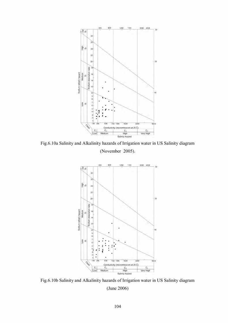
104
Fig.6.10a Salinity and Alkalinity hazards of Irrigation water in US Salinity diagram
(November 2005).
Fig.6.10b Salinity and Alkalinity hazards of Irrigation water in US Salinity diagram
(June 2006)

105
6.9.2.2 Residual Sodium Carbonate
Eaton (1957) suggested that the excess sum of carbonate and bicarbonate in
groundwater over the sum of calcium and magnesium also influences the suitability of
groundwater for irrigation.
RSC = )()( 33 MgCaHCOCO
where the concentrations are reported in meq/l. Water with RSC below 1.25 is good,
1.25-2.5 is marginal and above 2.5 is not suitable for irrigation purposes. The
classification of irrigation water according to the RSC value is presented in Table 6.4.
Table 6.4 Quality of groundwater based on residual sodium carbonate
RSC (meq/l) Remark on quality Post monsoon 2005 Pre monsoon 2006
Representing samples Representing samples
<1.25 Good 16 23
1.25-2.5 Doubtful 13 8
>2.5 Unsuitable 11 9
If RSC > 2.5, irrigation water may cause formation of salt peter (KNO3), locally known as
Reh.
6.10 Surface water Quality and Interaction with Groundwater
Seven surface water samples from rivers Yamuna and Krishni were analysed to
assess their relationship with the groundwater regime. The samples from Krishni river
show very high concentrations HCO3-, SO4
-, Na+ and K+. The TDS values, consequently,
are higher as well (Appendix-VIIIA & VIIIB).
The four Yamuna river samples with the exception of sample Y4 show good
correlation between Cl-/Na+ and HCO3- /Ca2++Mg2+ and have moderate TDS values of
400 and 500 mg/l. Strikingly high TDS value of >1000 mg/l is recorded for sample Y4 at
the down reaches.
The groundwater samples from the vicinity of Krishni River shows higher
concentration of HCO3-, SO4
-, Na+, K+, Ca+, Mg+. The higher concentration is attributed
to the seepage from drains, discharging the industrial effluent to Krishni River. Pollutants
enter in to the shallow aquifer through downward percolation, effluent draining
downward to the water table and further lateral movement below water table. The
impressions of saline waste water disposal of paper mill situated at Sikka village can be
106
seen in the groundwater sample taken from the same location. Here discharge from paper
mill flows through the unlined drain long distance before joining Krishni River.
A set of twelve trace elements i.e. Cr, Mn, Fe, Al, Pb, Ni, Co, Cu, Zn, As, Se and
Cd was analyzed in surface water sample of Yamuna-Krishni sub basin. The
concentration of Ni, Co, Cu, Zn, As, Se, and Cd are within the permissible limit
(Appendix IX C). The surface water samples have Cr, Mn, Pb and Fe concentrations
more than permissible limit which was collected from river Krishni at location Bhanera
and from Kandela drain i.e. 0.1142 to 0.1607, 0.423 to 0.4658 and 2.351 to 2.732 mg/l,
respectively.
6.11 Analysis of Effluent of Sugar Mill
Field survey reveals that a number of sugar mills and paper factories are
discharging their effluent in to the river Krishni in the upper reaches of the study area. A
sugar factory is a seasonal industry. The schedule of operation varies from year to year
depending on the occurrence of monsoon and availability of sugarcane. Hence the source
of groundwater pollution flows only for the period of operation of the sugar factory. Two
sample were collected from the Shamli Sugar mill. Out of these two, one is effluent water
and the other is partially treated sample i.e. lagoon water (in the terminology used in
sugar industry). The major elements analysis is given in Appendix-X-A and trace
elements analysis in Appendix-X B.
Effluent water shows higher concentration of HCO3, SO4, NO3, Na, K, and Ca. In
partially treated (lagoon water) the concentrations of anion is much higher. Even CO3 is
present with concentration of 445 mg/l. The presence of CO3 is an interesting feature and
is related to high pH value of 9 causing dissociation of bicarbonate.
107
7 – PROJECT FINDINGS
Hydrogeology
The aquifer system (upto 122 m bgl) has been taken up for detailed study in the
present work. This aquifer is sub divided at places into two to three sub groups by
occurrence of sub regional clay beds. By and large, the aquifer down to 122 m
appears to merge with each other and behave as a single bodied aquifer. The aquifer is
composed of fine to coarse sand. The sand percent map reveal that granular zone attain a
maximum value of >80% in the central and southern part of the area.
The result of grain size analysis of sand samples collected from a depth of 25-45 m bgl,
shows that the effective grain size of sample ranges from 0.064 mm to 0.19 mm
indicating that grain size is very fine to fine. The result of uniformity coefficient reveals
that in general, the sample shows a value of uniformity coefficient <2, hence their
porosity is high.
Depth to water table varies between 5.76 to 21.96 m bgl and 5.18 to 21.02 m bgl in
June 2006 and November 2006, respectively. The water level fluctuations therefore
are substantial during this period.
During 2007, the water level varies between 4.62 to 21.14 m bgl and 4.9 to 21.53 m
bgl, in pre and post-monsoon periods, respectively. The water level rise during 2007
is insignificant and 70% of the well shows negative fluctuation.
Historical water levels of 14 permanent monitoring wells were analysed for long term
water level trend. Out of these wells 6 wells represent command area and 8 wells
represent non-command area. The entire hydrographs show declining trend. The
average rate of decline is 0.96 m/year and 0.81 m/year, respectively.
Fourteen bimonthly water levels monitoring points were selected and to analyse the
groundwater fluctuation trends in response to utilization pattern. Most of the observation
wells show gradual decline in water level from the month of Feb-07 to June-07. The
significant rise at the locations Kairana and Todda may be attributed to some local
recharge factors.
The water table contour maps have revealed that the movement of groundwater is, in
general, from NNE to SSW. Localized groundwater flows are also encountered which
108
is possibly because of varied stress applied to the groundwater regime. In general the
gradient varies from 2.2 m/km in the NE region to 0.4 m/km at SW region. The high rate
of groundwater abstraction from shallow farmer’s tubewells is mainly responsible for the
water table decline in the area and resulting in to the formation of two troughs. The
formation of a trough in the lower half of the study area has, seemingly, influenced
the general groundwater flow pattern.
The Eastern Yamuna canal replenishes groundwater through seepage and also act as a
groundwater divide almost throughout the area. The groundwater flow direction at the
left bank of canal is towards the Krishni river with an average hydraulic gradient of 1.25
m/km. While from its right bank the groundwater flows from NE-SW direction. A
groundwater mound has developed near Khandrauli village which is shedding water
from its eastern flank to the river Krishni and from its western flank towards Kairana
township.
The contour behaviour shows that the river Yamuna is contributing the aquifer system
and hence influent through out the area. The groundwater flow direction is towards the
river Krishni hence it is effluent in nature.
An Isopermeability map has been prepared using Logan’s approximation (1964)
approach. The permeability 30-40 m/day covers bulk of the area. The Upland area
between river Yamuna and Katha drain has the permeability value <30 m/day.
The hydraulic conductivity of aquifer materials was also determined by constant head
Permeameter. The values obtained by Permeameter ranges from 1.01 m/day to 7.7 m/day.
The permeability values obtained by Permeameter are lower than the pumping test
values. The possible reason for low values is that the sand samples represent shallow
depth and the size of sand tested varies from very fine to fine. Moreover, the natural setup
is also altered because of compaction of the sand grains in confined environment.
Specific yield of 0.15-0.23 is used in and adjoining part of the study area by several
workers. However, for the present study specific yield of 0.16 is taken.
A long duration and 8 short duration pumping test result shows that the aquifer
parameters like Transmissivity and Hydraulic conductivity varies between 1265-4003
m2/day and 9.8-26.6 m/day, respectively.
109
Estimation of Dynamic Groundwater Resource
The results of the groundwater budget for two successive years i.e. June 2006 to May
2007 and June 2007 to May 2008, shows that the total recharge to the sub-basin is 427.79
MCM, 393.65 MCM and total discharge from the sub-basin is 478.48 MCM, 493.13
MCM thus, leaving a deficit balance of 50.69 MCM, 99.48 MCM and the stage of
groundwater development are worked out 111% and 125% respectively, which put the
sub-basin into over-exploited category.
The unplanned and massive groundwater exploitation is creating multifarious problems,
in the study area particularly in non-command area of the sub-basin. The water level is
very deep and has acquired a declining trend. As rainfall serves a major recharge
component, irregularity or delay in the monsoon, may lead to the scarcity of groundwater
in the area.
The uncertainties lie with the estimation of various components of groundwater budget,
owing to the limitations in the assessment methodology, as well as uncertainties in the
data. Thus, further efforts may be done to minimize the computational errors.
Groundwater Flow Modelling
Visual MODFLOW 4.1 (PM 4.1) is used in this study to simulate the groundwater flow
for steady and transient conditions, to forecast the future changes that occurred under
different stresses and also to investigate scenario of additional groundwater recharge to
evaluate their effect on the water table. The time period of November 2006 is taken as
initial state for steady state model calibration. Model calibration for steady state condition
shows good agreement between observed and simulated initial water level contours.
Transient state model calibration is carried out for the period June 1999 to June 2007.
Water level data of June 1999 was used as initial heads for the transient calibration.
Transient state calibration also shows good agreement between observed and calibrated
heads.
The sensitivity of the model to input parameters was tested by varying only the
parameters of interest over a range of values, and monitoring the response of the model
by determining the root mean square error of the simulated heads compared to the
measured heads.
110
Three scenarios have been considered to predict aquifer responses under different
conditions of groundwater abstraction and additional recharge through distributary and
drain in deficit areas. All the three prediction scenarios were chosen so as the situation is
acceptable with in the study area.
According to prediction scenario 1 i.e. with assumed 20% increased groundwater
abstraction rate the maximum drawdown will reach 10 m in the year 2014. The area in
close vicinity to river Krishni shows high decline rate as four observation wells have
gone dry in this scenario. The minimum drawdown is observed in the area close to river
Yamuna. In second scenario the rainfall is reduced by 20% and groundwater abstraction
was kept same as scenario 1. This shows that the maximum drawdown is very high (10
m). In this scenario, the area close to Krishni and southern part of the study area has
observed decline in water levels as envisaged by dewatering of shallow aquifer at five
locations. The third prediction scenario pertains to the situation, where additional
recharge is given to Kairana distributary and its irrigation channels. In this scenario, the
extent of dry cells has become smaller after the induced recharge. Thus, to mitigate the
water table decline, artificial recharge and conjunctive use of water is suggested.
Groundwater Vulnerability Assessment
The vulnerability index range from 140 to 180 and is classified into four classes i.e 140-
150, 150-160, 160-170 and 170-180 corresponding to low, medium, high and very high
vulnerability zones, respectively. The groundwater vulnerability potential map shows that
bulk of the area is covered by high to very high vulnerable zone followed by medium and
low vulnerable zones. Ironically, all major townships like Shamli, Kairana and Kandhala
are located in high to very high vulnerability zones. The vulnerability map thus generated
helps in identifying areas which are more likely to be susceptible to groundwater
contamination relative to one another.
Hydrogeochemistry
An attempt has also been made to evaluate and determine the possible factors controlling
variation in groundwater chemistry and to infer possible changes that occur in two time
periods that is post and premonsoon groundwater quality. The groundwater shows
strikingly high TDS concentration which seems to acquire increasing trend with time.
The unique chemical characteristic of the groundwater is the outcome of several natural
111
and anthropogenic processes. A chemical classification of groundwater was attempted on
the L-L diagram and identified four major group characterized by distinct chemical
compositions. The four major types of groundwater in the area are; HCO3-SO4 type, Cl-
SO4 type, HCO3 type, and SO4 type. Ion exchange and simple dissolution reactions help
in carving out the present shape to groundwater chemistry. The reaction involved in the
humic zone and dissolution of kankar, accumulation of salts through evaporation are also
affecting the hydrochemical regime. The anthropogenic factors affecting the groundwater
are application of fertilizers and manures and pollution from industrial effluents. The
groundwater regime is affected significantly and the meteoric signatures have been
completely obliterated. The high concentration of SO4-, HCO3
- and Na+ is of particular
concern. The concentrations of NO3-, F-, Fe and Pb in few groundwater samples are
above the permissible limit and may pose health hazards on human consumptions.
Broadly speaking, the groundwater is suitable for irrigation and drinking purposes with
few exceptions.
112
9. Conclusions / Recommendations
(i) Conclusions
This being a research project, a pilot area was taken for study, apply the existing techniques
in the best possible way by minimizing the assumptions and approximations and developing
the procedures and techniques using new aspects that were suitable to match the specific
condition. The detailed study carried out in the area sets an example for the similar areas as
well as reduces the uncertainties in the conclusions and recommendations. Specific details
are furnished below.
1. The area has experienced growth in population and hence in the water demand that
has put increased stress on the groundwater system.
2. All the available information on the hydraulic parameters and also determined from
the experiments in the project have been analysed and integrated in the model.
However, the grain size analyses confirm the presence of Alluvial aquifers and flow
system is such that the river Yamuna is influent throughout the area and for the entire
period of study. This is due to increase in groundwater pumping and reduction of the
base flow.
3. The two consecutive years groundwater balance has shown negative water balance
and that is alarming as well as produces the water level decline.
4. A unique contribution to this project has been the aquifer modeling by calibrating the
model in the steady conditions as well as for 8 years under transient conditions that is
usually rare and this has made the aquifer model producing the predicted result with
utmost certainty. In addition, sensitivity analyses has further given knowledge of the
areas and parameters for a careful monitoring in the future. The zonal water balance
that is possible only through aquifer modeling could reveal the specific situation in
the area and helped in suggesting the remedial measures.
5. The groundwater quality after hydrochemical analyses and interpretations found to be
acceptable for the time being but showing deteriorating trends with some important
constituents higher than the permissible limits.
113
The study has elaborated the groundwater situation in the area with details of the system
conditions with a greater certainty and is useful for further development and judicious
planning to avoid the groundwater crisis that was not otherwise possible.
(ii) Recommendations
In the past time, the demand-availability ratio was positive and managing the resource
was not a big deal but now a days when supply is running short and demand is escalating
high, management of groundwater resource is now becomes key issue. Several components
of the groundwater balance are time varying and further scientific investigations particularly
region wise converge of the accuracy and precision are needed. It is very clear from the
estimates that the development of groundwater in the region is intense and a slight change in
one of the components e.g. an increase in draft or a decrease in recharge hence further will
seriously deplete the groundwater storage. It is clear that the situation has reached to an
alarming stage which is likely to deteriorate further in the coming years. It is therefore clear
that strict controls on groundwater abstraction need to be introduced in order to manage the
groundwater resources of the Yamuna-Krishni sub-basin. Following recommendations and
consequences are suggested based on the findings.
Controlled Abstraction: In order to reduce total abstraction even the present rate of pumping
has to be carefully controlled. For example groundwater withdrawal could be reduced in non-
command areas where two groundwater troughs have been generated. It is suggested that
groundwater withdrawal along river Yamuna flood plains can be slightly increased.
Augmentation of water resources: Suitable measures for augmentation of groundwater
resources may be adopted e.g. artificial recharge may ease the situation in the study area
before the situation becomes unmanageable. However, emphasis must be put on demand
management as rainwater harvesting will reduce the runoff and further reduce the flow to the
rivers.
Development from deeper aquifer: The groundwater abstraction can be focused on deeper
aquifers. The study carried out by CGWB in alluvial parts of Central Ganga Plain have
revealed the existence of a huge reserve of groundwater in the deeper aquifer, which have not
been fully utilized. The thickness of the alluvium in the area exceeds 500 m and only a small
114
fraction of this is under active circulation due to prevailing shallow groundwater
development. Therefore, it is suggested that IInd and IIIrd aquifer should be taped.
Development of flood plain: Flood plains in the vicinity of rivers are good repositories of
groundwater. A planned management of groundwater in the flood plain aquifers offers an
excellent scope of its development to meet the additional requirement of water. The main
efforts, in this regard, are needed to make the groundwater available at the place of demand.
Restoring traditional groundwater structures: In the past, every village in western Uttar
Pradesh boasted of having ponds and community tanks which have been a very good source
of groundwater recharge, at least locally. Now, it was observed during the field surveys that
the ponds and tanks have disappeared due to encroachment by local people. This has retarded
the groundwater recharge of shallow aquifer. Thus revival of such structures is
recommended.
Improvement in Canal System: The present canal irrigation system in the study area is
untimely and restricted to the vicinity of main canal. The irrigation channels in the down
reaches do not receive water from the feeder canals and thus requires proper management
policy to ensure the availability of water at the tail ends of canal vis-à-vis irrigation channels.
Conjunctive use of surface and groundwater: Conjunctive use of surface water and
groundwater resources is the optimal method of obtaining maximum possible water
development the same has been tested and proved in the aquifer modelling
Protection of groundwater from pollution: It is suggested that the urban landfill, garbage
dumps and effluent channels should either have concrete floor or sheets of impervious film
be used to prevent leaching of pollutants in the water.
Stopping subsidized power supply: The pumping mainly depends on the electric supply. The
electric supply in the study area is at a very subsidized rate and due to this lot of water is
wasted. Moreover, frequent power theft instances also encourage farmers for indiscriminate
pumping. A water and energy nexus may be evolved in the further study.
People’s awareness: The public support is needed to implement groundwater management.
Institutional frameworks that enable effective participation of local users and communities in
the management processes are essential. It is also suggested that in the local languages of
115
region, seminars, posters presentations be arranged for educating the public of urban and
rural areas for judicious use of groundwater.
The awareness of farmers towards the groundwater recharge can prove an important
milestone in managing the groundwater resources.
Groundwater Legislation: A strict groundwater legislation using the scientitific studies such
as the present one should be brought in to regulate harnessing of groundwater resources.
10. How do the conclusions / recommendations compare with current thinking.
The present work is one of its kinds, as the groundwater budget is performed at micro
level, including all possible influential components of groundwater budget. Also, the river
aquifer interaction and other boundary flows were calculated using groundwater flow
modelling. Moreover the fact that the demand-supply ratio is escalating, it further
necessitates that the resource evaluation should be done more precisely. The precise account
of groundwater budget serves as the backbone of any groundwater management programme.
Thus, after detailed hydrogeological examination the study emphasizes upon groundwater
budget.
The present work can be extended as the sub-basin needs to be monitored for
groundwater conditions for some years. The dynamic resource of the sub-basin is being
exploited at an alarming rate. The groundwater is being harnessed continuously to cope up
with the rising demands. Moreover, the recharge to the system is decreasing day by day as
groundwater discharge exceeds the recharge, due to deficit rainfall. The applicability of
recommendations and their socio-economical impacts need to be analysed in the times to
come.
Any multidisciplinary scientific study for the evaluation of natural phenomenon
carries errors at some stages of assessment, thus improvements are always inevitable. The
lacunae may arise because of improper understanding of the system. It was nearly impossible
to assign observation well at known altitude location, the error arises as this may locally
change the flow pattern of the groundwater regime. Improvements are further possible in
groundwater budget, at the statistical level, like number of groundwater draft structures and
irrigation water applied may carry certain errors. The vertical leakage from the first aquifer
under consideration needs to be accounted for.
116
In addition, emphasis has in particular been laid on aquifer vulnerability and
hydrogeochemical aspects, such as, chemical types of groundwater, temporal and spatial
variation in chemical characteristics, chemical alteration trends of groundwater, factors
affecting the chemical quality. Again, the idea is to provide some clues to planners and
administrators to mitigate the problem of groundwater pollution.
11. Field tests conducted.
Following tests were conducted during field work
(i) Coordinates of the borewells were taken using GPS.
(ii) Repeat measurements to monitor the changes in water level, for post-monsoon
2005, pre-and post-monsoon 2006 and 2007 respectively in all the monitoring
wells
(iii) Bimonthly water level monitoring was also carried out from February 2007to
November 2008 at 14 selected monitoring wells.
. (iv) pH, Temperature and EC were measured at well site during sampling.
(v) The concentrations of NO3 and F were also determined at well site with the
help of portable kits.
12. Software generated, if any: No
Visual MODFLOW 4.1 P, were used for Numerical Modelling of Yamuna-
Krishni sub-basin.
13. Possibilities of any patents/copyrights. If so, then action taken in this regard: No
14. Suggestions for further work
There are following suggestions for further work.
Artificial recharge sites: Study for identification of site for Artificial Recharge.
Water level: Installation of Peizometre at micro level for monitoring the groundwater
level.
Further scientific investigations: Several components of the groundwater balance are
time-dependent and further scientific investigations (particularly region-wise) are
necessary in order to provide the required additional accuracy and precision.
Groundwater quality: It is possible that further pumping may lead to deterioration of
groundwater quality leading to its unsuitability as a drinking water source by the rural
population; further groundwater quality investigations are required.
117
Paper published from project
1. Izrar Ahmed and Rashid Umar (2009) Groundwater flow modelling of Yamuna –
Krishni interstream, a part of central Ganga Plain, Uttar Pradesh. J. Earth Syst.
Sci. 118. No.5, pp. 507-523
2. Rashid Umar, Izrar Ahmed and Fakhre Alam (2009) Mapping Groundwater
vulnerable zones using modified DRASTIC approach of an alluvial aquifer in
parts of Central Ganga Plain, Western Uttar Pradesh. J. Geol. Soc. India, vol.
73, pp.193-201.
3. Rashid Umar, Izrar Ahmed, Fakhre Alam and Mohammad Muqtada Khan (2009):
Hydrochemical Characteristics and seasonal variations in Groundwater
Quality of an alluvial aquifer in parts of Central Ganga Plain, Western Uttar
Pradesh, India. Environ. Geol. vol. 58. No. 6, pp. 1295-1300
4. Rashid Umar & Izrar Ahmed (2009) Sustainability of a shallow aquifer in
Yamuna-Krishni interstream region, Western Uttar Pradesh: a quantitative
assessment. Trends and Sustainability of Groundwater in Highly Stressed
Aquifer, Proc. of Symposium JS.2 IAHS publication 329 at the Joint IAHS &
IAH Convention, Hyderabad, India. pp.103-112
Ph.D Thesis:
Guided: One (Awarded)
118
REFERENCES
Agrawal RK (1977) Structure and tectonics of Indo-Gangetic plains. Geophysical Case
Histories of India. Assoc. Exploration Geophysicists, V.1, pp. 29-46.
Aller L, Lehr JH, Petty R, Bennett T (1987) Drastic : A standardized system to
evaluate Groundwater Pollution using Hydrogeologic setting. Jour Geol Soc of
India 29(1): 23-37
Anderson M.P. and Woessner WW. (2002) Applied groundwater Modeling-Simulation of
flow and Advective transport. Academic Press (Elsevier, USA) pp.341.
Anderson MP, Woessner WW (1992) Applied Groundwater Modeling. Academic Press, San
Diego.
APHA (1992) Standard methods for the examination of Water and Wastewater, 16th
edition, APHA, Washington, D.C.
Bajpai V (1989) Surface and Subsurface evidences of Neotectonic and aquifer disposition
in Central alluvium terrain of Kanpur and Unnao region in Uttar Pradesh, India.
Photonirvachak. Jour. Indian Soc. Remote Sensing, V.17, pp.47-53
Balasubramanian (2001) Overview of Groundwater Models, Modelling in Hydrogeology
(Edt. Book),Elango,L.and Jayakumar, R., Allied Publishers Limited (Mumbai).pp.17-
24.
Barlow PM, Harbaugh AW (2006) USGS Directions in MODFLOW Development.
Groundwater 44(6):771-774.
Bhatnagar NC, Agashe RM, Mishra AK (1982) “Subsurface Mapping of Aquifer System”
Water balance study of Upper Yamuna Basin, Section-Hydrogeology, Technical
report No.2, Upper Yamuna Project,CGWB, NW region, Chandigarh.
Bhosle B, Prakash B, Awasthi AK, Singh VN, Singh S (2007) Remote sensing-GIS and
GPR studies of two active faults, Western Gangetic Plains, India. Journal of
Applied Geophysics 61:155-164.
BIS (1991) Indian standard specifications for drinking water, B.S. 10500
Chakrapani GJ (2005) Major and Trace element geochemistry in upper Ganga river in the
Himalayas, India, Environ Geol 48: 189-201.
Comly HH (1945) Cyanosis in infants caused by nitrates in well water. J Am Mwd Assos
129:12-114.
119
Coudrain–Ribstein A, Pratx B, Talbi A, Jusserand C (1998) Is the evaporation from
pheratic aquifers in arid zones independent of the Soil characteristics?
C.R.Acad.Sci.Paris, Sciences de la Terra et des Planetes, 326:159-165
Deutsch W J (1997) Groundwater Geochemistry; Funadamentals and applications to
Contamination, Lewis Publishers, New-York,221pp
Domenico PA, Schwartz FW (1997) Physical and Chemical Hydrogeology, IInd Edtn.
John Wiley and Sons, INC 495p.
Drever JΙ (1982) The geochemistry of natural waters. Prantice Hall, England Cliffs, NJ.
Earth Summit (1992) Agenda 21 Programme of Action of Sustainable Development,
UNCED, Rio de Janeiro, Brazil, pp 174-175.
Eaton FM (1957) Significance of carbonate in Irrigation water, Soil Sci., Vol.69,
No.2, pp.123-133.
Edet, A.E., Merkel, B.J. and Offiong, O.E., (2003). Trace element hydrochemical
assessment of the calabar coastal plain aquifer, southeastern Nigeria using statistical
methods. Environ Geol 44: pp.137-149.
Freeze RA and Cherry AJ (1979) Groundwater, Prantice Hall, Inc. New Jersey, pp 262-
265.
Gilly G, Corrao G, Favilli S (1984) Concentrations of nitrates in drinking water and
incidence of gastric carcinomas. First descriptive study of the Piemonate Region,
Italy. Sci Total Environ 34:35-37.
Gupta CP, Ahmad S, Rao, VVSG (1985) Conjunctive utilization of Surface Water and
Groundwater to arrest the water level decline in an alluvial aquifer. J Hydrol
76:351-361.
Handa, B.K., (1986). Trace elements content of groundwater in the basaltic rocks in some
parts of Indian peninsula. In: Hydrogeology of Volcanic terrains, Power, K.B and
Thigale, S.S (Eds.), University of Poona, Pune, pp.83-104.
Herlinger, JR.R. and Viero, A.P. (2007) Groundwater vulnerability assessment in coastal
plain of Rio Grande do Sul State, Brazil, using drastic and adsorption capacity of
soils. Environ. Geol., v.52, pp.819-829.
120
Hsu KC, Wang CH, Chen KC, Chen CT, Ma KW (2007) Climate-induced hydrological
impacts on the groundwater system of the Pingtung Plain, Taiwan. Hydrogeol
J,V.15(5): 903-913.
Hussain MH, Singhal DC, Joshi H, Kumar S (2006) Assessment of Groundwater
vulnerability in a tropical alluvial interfluves, India, Bhu-Jal News Jour., No.1-4: 31-
43.
Jyrkama MI, Skyes JF, Normani SD (2002) Recharge estimation of transient groundwater
modeling. Groundwater 40(6):638-648.
Karanth KR (1987) Groundwater Assessment, Development and Management. Tata
McGraw Hill Publishing Company Limited, New Delhi, pp 576-638.
Karunakaran C, Rangarao A (1979) Status of exploration for hydrocarbons in the Himalayan
region-contribution to stratigraphy and structure. Geol.Surv.India Pub. V.41, pp.1-66.
Kennett-Smith A, Narayan K, Walker G (1996) Calibration of a Groundwater model for the
upper south east of South Australia. Div. report 96-2.CSIRO Division of Water
Resources, Canberra, Australia.
Khan AM (1992) Report on systematic Hydrogeological Surveys in parts of
Muzaffarnagar District, Uttar Pradesh, CGWB (Northern region).
Kruseman GP, Ridder NA (1970) Analysis and evaluation of pumping test data, Bull 11,
Intl. Inst. for land Reclamation and improvement, Wegeningen Netherland.
Langelier W F, Ludwig H F (1942) Graphic method for indicating the mineral character of
natural water J Am Water Works Assoc 34(3):335-352
Logan (1964) Estimating transmissivity from routine production tests of water wells,
Groundwater 2(1):35-37.
McDonald MG, Harbaugh AW (1988) A modular three dimensional finite-difference
groundwater flow model. USGS Open File Report 83-875.USGS, Washington,
D.C.
Ministry of Water Resources (1997) Report of the groundwater resource estimation
committee-Groundwater resource estimation methodology, Government of India,
New Delhi.
121
Mohan, S. (2001) Groundwater Water Modelling: Issues and Requirements, Modelling in
Hydrogeology, (Edt. Book), Elango, L. and Jayakumar, R., Allied Publishers Limited
(Mumbai).pp.3-16.
National Bank for Agriculture and Rural Development (2006) Review of
Methodologies for Estimation of Groundwater Resources in India.
Nevill HR (1903) District Gazetteer of Muzaffarnagar.
Onta P.R., Dasgupta, A. and Harboe, R. (1991) Multistep planning model for conjunctive
use of surface-water and groundwater resources, Journal of Water Resources
Planning and Management 117(6):662-678.
Qinghai G, Yanxin W, Xubo G, Teng M (2007) A new model (DRARCH) for assessing
groundwater vulnerability to arsenic contamination at basin scale: a case study in
Taiyuan basin, northern China, Environ Geol 52:923-932.
Raja RK, Rawat SN, Chhabra SS (1989) In: International Workshop on Appropriate
Methodologies and management of Groundwater Resources in developing countries
(Eds: Gupta CP, Ahmed S, Rao VVSG, Thangarajan M), published by Oxford and
IBH publishing co. pvt Limited.pp:119-130.
Rao MBR (1973) The subsurface geology of the Indo-Gangetic Plains, J Geol Soc
India 14:217-242.
Reichard E.G. (1995) Groundwater surface water management with stochastic surface
water supplies-A simulation optimization approach. Water Resources Research
31(11):2845-2865.
Richards LA (1954) Diagnosis and improvement of saline alkali soils. US department of
agriculture, Hand Boock 60, pp 160
Rushton K 2006 Representation in regional models of saturated river-aquifer interaction for
gaining losing rivers, J. Hydrol. 334, 262-281.
Sastri VV, Bhandari LL, Raju ATR, Datta AK (1971) Tectonic framework and
subsurface stratigraphy of the Ganga basin. J Geol Soc India 12(3):222-233.
Sawyer CN, Mc Carty PL (1967) Chemistry for sanitary, IV Edtn., McGraw Hill, New
York, 518p.
122
Santhilkumar M, Elango L (2004) Three dimensional mathematical model to simulate
groundwater flow in the lower Palar River basin, southern India. Hydrogeology
Journal.V12(3):197-208.
Singh IB (1996) Geological evolution of Ganga Plain-An overview. Jour of the
Palaeontological Society of India 41:99-137.
Singh IB (2004) Late Quaternary History of the Ganga Plain. J Geol Soc India 64:431-
454.
Subramanian V, Saxena K (1983) Hydrogechemistry of groundwater in the Delhi region of
India, relation of water quality and quantity. In: Proceedings of the Hamberg
symposium IAHS publication no. 146, pp 307-316.
Survey of India (2003) District map of Muzaffarnagar.
Umar R, Absar A (2003) Chemical characteristics of groundwater in parts of the Ghambhir
River basin, Bharatpur District, Rajasthan, India, Environ Geol 44:535- 544.
Umar R, Ahmed I (2007) Hydrochemical characteristics of Groundwater in parts of
Krishni-Yamuna Basin, Muzaffarnagar district, U.P., J Geol Soc India 69:989-
995.
USGS (1993) National water Summary-1990- 1991: Stream Water Quality U.S.Geol.
Surv. Water Supply paper No. 2400, 590p.
U.S.Salinity Laboratory Staff (USSL), (1954) Diagonosis and improvement of salinity and
alkaline soils, U.S.D.A., Hand Book No. 60, pp 160.
Valdiya KS (1980) Geology of the Kumaun Lesser Himalaya. WIHG, Dehra Dun, India
Varni MR, Usunoff EJ (1999) Simulation of regional scale groundwater flow in the azul
River Basin, Buenos Aires province, Argentina. Hydrogeol J 7(2):180-187.
Varun DP (1980) District Gazetteer of Muzaffarnagar.
Vias JM, Andreo B, Perles MJ, Carrasco F (2005) A comparative study of four
schemes for groundwater vulnerability mapping in a diffuse flow carbonate
aquifer under Mediterranean climatic conditions. Environ Geol 47:586-595
Vrba J, Zeporozec A (1994) Guidebook on mapping Groundwater vulnerability,
International contributions to Hydrogeology 16:129p.
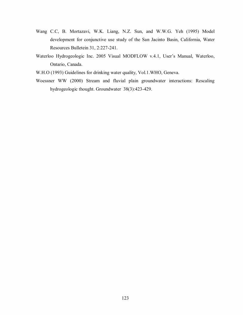
123
Wang C.C, B. Mortazavi, W.K. Liang, N.Z. Sun, and W.W.G. Yeh (1995) Model
development for conjunctive use study of the San Jacinto Basin, California, Water
Resources Bulletein 31, 2:227-241.
Waterloo Hydrogeologic Inc. 2005 Visual MODFLOW v.4.1, User’s Manual, Waterloo,
Ontario, Canada.
W.H.O (1993) Guidelines for drinking water quality, Vol.1.WHO, Geneva.
Woessner WW (2000) Stream and fluvial plain groundwater interactions: Rescaling
hydrogeologic thought. Groundwater 38(3):423-429.
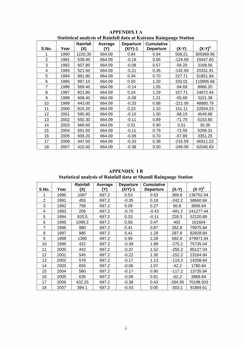
i
APPENDIX I A Statistical analysis of Rainfall data at Kairana Raingauge Station
S.No. Year Rainfall
(X) Average
(Y) Departure
(X/Y)-1 Cumulative Departure (X-Y) (X-Y)
2
1 1990 1220.30 664.09 0.84 0.84 556.21 309369.56
2 1991 539.40 664.09 -0.19 0.65 -124.69 15547.60
3 1992 607.80 664.09 -0.08 0.57 -56.29 3168.56
4 1993 521.50 664.09 -0.21 0.35 -142.59 20331.91
5 1994 891.80 664.09 0.34 0.70 227.71 51851.84
6 1995 997.10 664.09 0.50 1.20 333.01 110895.66
7 1996 569.40 664.09 -0.14 1.05 -94.69 8966.20
8 1997 821.80 664.09 0.24 1.29 157.71 24872.44
9 1998 608.40 664.09 -0.08 1.21 -55.69 3101.38
10 1999 443.00 664.09 -0.33 0.88 -221.09 48880.79
11 2000 815.20 664.09 0.23 1.10 151.11 22834.23
12 2001 595.90 664.09 -0.10 1.00 -68.19 4649.88
13 2002 592.30 664.09 -0.11 0.89 -71.79 5153.80
14 2003 669.60 664.09 0.01 0.90 5.51 30.36
15 2004 591.50 664.09 -0.11 0.79 -72.59 5269.31
16 2005 606.20 664.09 -0.09 0.70 -57.89 3351.25
17 2006 447.50 664.09 -0.33 0.38 -216.59 46911.23
18 2007 415.00 664.09 -0.38 0.00 -249.09 62045.83
APPENDIX I B Statistical analysis of Rainfall data at Shamli Raingauge Station
S.No. Year Rainfall
(X) Average
(Y) Departure
(X/Y)-1 Cumulative Departure (X-Y) (X-Y)
2
1 1990 1067 697.2 0.53 0.53 369.8 136752.04
2 1991 455 697.2 -0.35 0.18 -242.2 58660.84
3 1992 758 697.2 0.09 0.27 60.8 3696.64
4 1993 206 697.2 -0.70 -0.43 -491.2 241277.44
5 1994 925.5 697.2 0.33 -0.11 228.3 52120.89
6 1995 1099.2 697.2 0.58 0.47 402 161604
7 1996 980 697.2 0.41 0.87 282.8 79975.84
8 1997 985 697.2 0.41 1.29 287.8 82828.84
9 1998 1390 697.2 0.99 2.28 692.8 479971.84
10 1999 422 697.2 -0.39 1.89 -275.2 75735.04
11 2000 442 697.2 -0.37 1.52 -255.2 65127.04
12 2001 545 697.2 -0.22 1.30 -152.2 23164.84
13 2002 578 697.2 -0.17 1.13 -119.2 14208.64
14 2003 655 697.2 -0.06 1.07 -42.2 1780.84
15 2004 580 697.2 -0.17 0.90 -117.2 13735.84
16 2005 635 697.2 -0.09 0.81 -62.2 3868.84
17 2006 432.25 697.2 -0.38 0.43 -264.95 70198.503
18 2007 394.1 697.2 -0.43 0.00 -303.1 91869.61
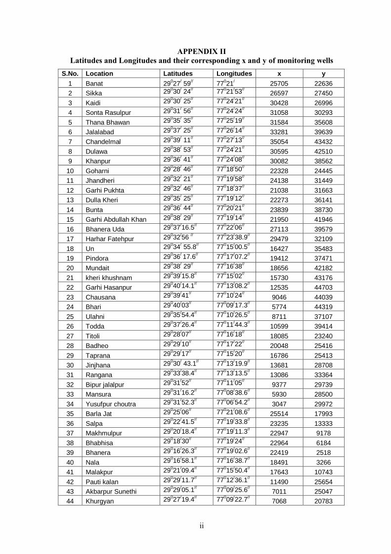
ii
APPENDIX II Latitudes and Longitudes and their corresponding x and y of monitoring wells
S.No. Location Latitudes Longitudes x y
1 Banat 29027
/ 59
// 77
021
/ 25705 22636
2 Sikka 29030
/ 24
// 77
021
/53
// 26597 27450
3 Kaidi 29030
/ 25
// 77
024
/21
// 30428 26996
4 Sonta Rasulpur 29031
/ 56
// 77
024
/24
// 31058 30293
5 Thana Bhawan 29035
/ 35
// 77
025
/19
// 31584 35608
6 Jalalabad 29037
/ 25
// 77
026
/14
// 33281 39639
7 Chandelmal 29039
/ 11
// 77
027
/13
// 35054 43432
8 Dulawa 29038
/ 53
// 77
024
/21
// 30595 42510
9 Khanpur 29036
/ 41
// 77
024
/08
// 30082 38562
10 Goharni 29028
/ 46
// 77
018
/50
// 22328 24445
11 Jhandheri 29032
/ 21
// 77
019
/58
// 24138 31449
12 Garhi Pukhta 29032
/ 46
// 77
018
/37
// 21038 31663
13 Dulla Kheri 29035
/ 25
// 77
019
/12
// 22273 36141
14 Bunta 29036
/ 44
// 77
020
/21
// 23839 38730
15 Garhi Abdullah Khan 29038
/ 29
// 77
019
/14
// 21950 41946
16 Bhanera Uda 29037
/16.5
// 77
022
/06
// 27113 39579
17 Harhar Fatehpur 29032
/56
// 77
023
/38.9
// 29479 32109
18 Un 29034
/ 55.8
// 77
015
/00.5
// 16427 35483
19 Pindora 29036
/ 17.6
// 77
017
/07.2
// 19412 37471
20 Mundait 29038
/ 29
// 77
016
/38
// 18656 42182
21 kheri khushnam 29039
/15.8
// 77
015
/02
// 15730 43176
22 Garhi Hasanpur 29040
/14.1
// 77
013
/08.2
// 12535 44703
23 Chausana 29039
/41
// 77
010
/24
// 9046 44039
24 Bhari 29040
/03
// 77
009
/17.3
// 5774 44319
25 Ulahni 29035
/54.4
// 77
010
/26.5
// 8711 37107
26 Todda 29037
/26.4
// 77
011
/44.3
// 10599 39414
27 Titoli 29028
/07
// 77
016
/18
// 18085 23240
28 Badheo 29029
/10
// 77
017
/22
// 20048 25416
29 Taprana 29029
/17
// 77
015
/20
// 16786 25413
30 Jinjhana 29030
/ 43.1
// 77
013
/19.9
// 13681 28708
31 Rangana 29033
/38.4
// 77
013
/13.5
// 13086 33364
32 Bipur jalalpur 29031
/52
// 77
011
/05
// 9377 29739
33 Mansura 29031
/16.2
// 77
008
/38.6
// 5930 28500
34 Yusufpur choutra 29031
/52.3
// 77
006
/54.2
// 3047 29972
35 Barla Jat 29025
/06
// 77
021
/08.6
// 25514 17993
36 Salpa 29022
/41.5
// 77
019
/33.8
// 23235 13333
37 Makhmulpur 29020
/18.4
// 77
019
/11.3
// 22947 9178
38 Bhabhisa 29018
/30
// 77
019
/24
// 22964 6184
39 Bhanera 29016
/26.3
// 77
019
/02.6
// 22419 2518
40 Nala 29016
/58.1
// 77
016
/38.7
// 18491 3266
41 Malakpur 29021
/09.4
// 77
015
/50.4
// 17643 10743
42 Pauti kalan 29029
/11.7
// 77
012
/36.1
// 11490 25654
43 Akbarpur Sunethi 29029
/05.1
// 77
009
/25.6
// 7011 25047
44 Khurgyan 29027
/19.4
// 77
009
/22.7
// 7068 20783
iii
45 Khera 29024
/51.9
// 77
009
/41.6
// 7138 17550
46 Mawi 29022
/39.7
// 77
009
/17.7
// 7249 13492
47 Saipat 29020
/28.8
// 77
009
/58
// 8179 9899
48 Jharkhedi 29022
/22.1
// 77
011
/50.1
// 11188 13157
49 Kairana 29023
/50.3
// 77
012
/49
// 12475 16137
50 Kandela 29025
/44.8
// 77
014
/40.8
// 15150 19570
51 Bhoora 29027
/00.6
// 77
012
/34.5
// 12011 21639
52 Kaserwa Khurd 29027
/36.5
// 77
015
/23.8
// 16630 22170
53 Khandrauli 29023
/12
// 77
016
/49
// 19017 14645
54 Lilaun 29025
/39
// 77
017
/28.5
// 20154 18440
55 Erti 29024
/25
// 77
015
/43
// 17007 16592
56 Gangeru 29018
/42
// 77
013
/9.5
// 12888 6665
57 Unchagaon 29021
/28
// 77
013
/48
// 13769 11252
58 Shamli 29027
/10.9
// 77
018
/37.9
// 21731 21615
59 Kandhla 29019
/15
// 77
016
/52
// 16830 7425
60 Garhi Rakha 29016
/10
// 77
011
/45
// 10500 4650
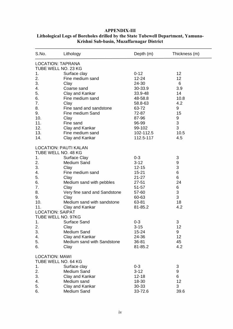
iv
APPENDIX-III Lithological Logs of Boreholes drilled by the State Tubewell Department, Yamuna-
Krishni Sub-basin, Muzaffarnagar District S.No. Lithology Depth (m) Thickness (m) LOCATION: TAPRANA TUBE WELL NO. 23 KG 1. Surface clay 0-12 12 2. Fine medium sand 12-24 12 3. Clay 24-30 6 4. Coarse sand 30-33.9 3.9 5. Clay and Kankar 33.9-48 14 6. Fine medium sand 48-58.8 10.8 7. Clay 58.8-63 4.2 8. Fine sand and sandstone 63-72 9 9. Fine medium Sand 72-87 15 10. Clay 87-96 9 11. Fine sand 96-99 3 12. Clay and Kankar 99-102 3 13. Fine medium sand 102-112.5 10.5 14. Clay and Kankar 112.5-117 4.5 LOCATION: PAUTI KALAN TUBE WELL NO. 48 KG 1. Surface Clay 0-3 3 2. Medium Sand 3-12 9 3. Clay 12-15 3 4. Fine medium sand 15-21 6 5. Clay 21-27 6 6. Medium sand with pebbles 27-51 24 7. Clay 51-57 6 8. Very fine sand and Sandstone 57-60 3 9. Clay 60-63 3 10. Medium sand with sandstone 63-81 18 11. Clay and Kankar 81-85.2 4.2 LOCATION: SAIPAT TUBE WELL NO. 97KG 1. Surface Sand 0-3 3 2. Clay 3-15 12 3. Medium Sand 15-24 9 4. Clay and Kankar 24-36 12 5. Medium sand with Sandstone 36-81 45 6. Clay 81-85.2 4.2 LOCATION: MAWI TUBE WELL NO. 64 KG 1. Surface clay 0-3 3 2. Medium Sand 3-12 9 3. Clay and Kankar 12-18 6 4. Medium sand 18-30 12 5. Clay and Kankar 30-33 3 6. Medium Sand 33-72.6 39.6
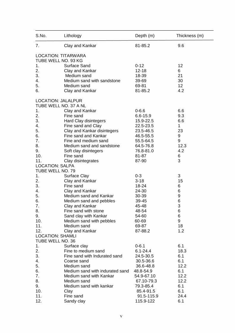
v
S.No. Lithology Depth (m) Thickness (m) 7. Clay and Kankar 81-85.2 9.6 LOCATION: TITARWARA TUBE WELL NO. 93 KG 1. Surface Sand 0-12 12 2. Clay and Kankar 12-18 6 3. Medium sand 18-39 21 4. Medium sand with sandstone 39-69 30 5. Medium sand 69-81 12 6. Clay and Kankar 81-85.2 4.2 LOCATION: JALALPUR TUBE WELL NO. 37 A NL 1. Clay and Kankar 0-6.6 6.6 2. Fine sand 6.6-15.9 9.3 3. Hard Clay disintegers 15.9-22.5 6.6 4. Fine sand and Clay 22.5-23.5 1 5. Clay and Kankar disintegers 23.5-46.5 23 6. Fine sand and Kankar 46.5-55.5 9 7. Fine and medium sand 55.5-64.5 9 8. Medium sand and sandstone 64.5-76.8 12.3 9. Soft clay disintegers 76.8-81.0 4.2 10. Fine sand 81-87 6 11. Clay disintegrates 87-90 3 LOCATION: SALPA TUBE WELL NO. 79 1. Surface Clay 0-3 3 2. Clay and Kankar 3-18 15 3. Fine sand 18-24 6 4. Clay and Kankar 24-30 6 5. Medium sand and Kankar 30-39 9 6. Medium sand and pebbles 39-45 6 7. Clay and Kankar 45-48 3 8. Fine sand with stone 48-54 6 9. Sand clay with Kankar 54-60 6 10. Medium sand with pebbles 60-69 9 11. Medium sand 69-87 18 12. Clay and Kankar 87-88.2 1.2 LOCATION: SHAMLI TUBE WELL NO. 36 1. Surface clay 0-6.1 6.1 2. Fine to medium sand 6.1-24.4 18.3 3. Fine sand with Indurated sand 24.5-30.5 6.1 4. Coarse sand 30.5-36.6 6.1 5. Medium sand 36.6-48.8 12.2 6. Medium sand with indurated sand 48.8-54.9 6.1 7. Medium sand with Kankar 54.9-67.10 12.2 8. Medium sand 67.10-79.3 12.2 9. Medium sand with kankar 79.3-85.4 6.1 10. Clay 85.4-91.5 6.1 11. Fine sand 91.5-115.9 24.4 12. Sandy clay 115.9-122 6.1
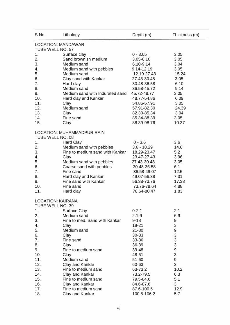
vi
S.No. Lithology Depth (m) Thickness (m) LOCATION: MANDAWAR TUBE WELL NO. 57 1. Surface clay 0 - 3.05 3.05 2. Sand brownish medium 3.05-6.10 3.05 3. Medium sand 6.10-9.14 3.04 4. Medium sand with pebbles 9.14-12.19 3.05 5. Medium sand 12.19-27.43 15.24 6. Clay sand with Kankar 27.43-30.48 3.05 7. Hard clay 30.48-36.58 6.10 8. Medium sand 36.58-45.72 9.14 9. Medium sand with Indurated sand 45.72-48.77 3.05 10. Hard clay and Kankar 48.77-54.86 6.09 11. Clay 54.86-57.91 3.05 12. Medium sand 57.91-82.30 24.39 13. Clay 82.30-85.34 3.04 14. Fine sand 85.34-88.39 3.05 15. Clay 88.39-98.76 10.37 LOCATION: MUHAMMADPUR RAIN TUBE WELL NO. 08 1. Hard Clay 0 - 3.6 3.6 2. Medium sand with pebbles 3.6 - 18.29 14.6 3. Fine to medium sand with Kankar 18.29-23.47 5.2 4. Clay 23.47-27.43 3.96 5. Medium sand with pebbles 27.43-30.48 3.05 6. Coarse sand with pebbles 30.48-36.58 6.1 7. Fine sand 36.58-49.07 12.5 8. Hard clay and Kankar 49.07-56.38 7.31 9. Fine sand with Kankar 56.38-73.76 17.38 10. Fine sand 73.76-78.64 4.88 11. Hard clay 78.64-80.47 1.83 LOCATION: KAIRANA TUBE WELL NO. 39 1. Surface Clay 0-2.1 2.1 2. Medium sand 2.1-9 6.9 3. Fine to med. Sand with Kankar 9-18 9 4. Clay 18-21 3 5. Medium sand 21-30 9 6. Clay 30-33 3 7. Fine sand 33-36 3 8. Clay 36-39 3 9. Fine to medium sand 39-48 9 10. Clay 48-51 3 11. Medium sand 51-60 9 12. Clay and Kankar 60-63 3 13. Fine to medium sand 63-73.2 10.2 14. Clay and Kankar 73.2-79.5 6.3 15. Fine to medium sand 79.5-84.6 5.1 16. Clay and Kankar 84.6-87.6 3 17. Fine to medium sand 87.6-100.5 12.9 18. Clay and Kankar 100.5-106.2 5.7
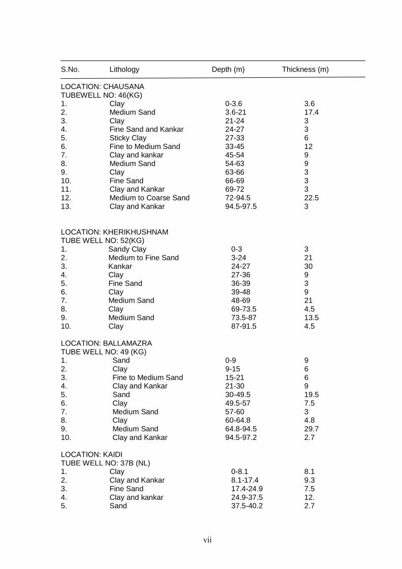
vii
S.No. Lithology Depth (m) Thickness (m) LOCATION: CHAUSANA TUBEWELL NO: 46(KG) 1. Clay 0-3.6 3.6 2. Medium Sand 3.6-21 17.4 3. Clay 21-24 3 4. Fine Sand and Kankar 24-27 3 5. Sticky Clay 27-33 6 6. Fine to Medium Sand 33-45 12 7. Clay and kankar 45-54 9 8. Medium Sand 54-63 9 9. Clay 63-66 3 10. Fine Sand 66-69 3 11. Clay and Kankar 69-72 3 12. Medium to Coarse Sand 72-94.5 22.5 13. Clay and Kankar 94.5-97.5 3 LOCATION: KHERIKHUSHNAM TUBE WELL NO: 52(KG) 1. Sandy Clay 0-3 3 2. Medium to Fine Sand 3-24 21 3. Kankar 24-27 30 4. Clay 27-36 9 5. Fine Sand 36-39 3 6. Clay 39-48 9 7. Medium Sand 48-69 21 8. Clay 69-73.5 4.5 9. Medium Sand 73.5-87 13.5 10. Clay 87-91.5 4.5 LOCATION: BALLAMAZRA TUBE WELL NO: 49 (KG) 1. Sand 0-9 9 2. Clay 9-15 6 3. Fine to Medium Sand 15-21 6 4. Clay and Kankar 21-30 9 5. Sand 30-49.5 19.5 6. Clay 49.5-57 7.5 7. Medium Sand 57-60 3 8. Clay 60-64.8 4.8 9. Medium Sand 64.8-94.5 29.7 10. Clay and Kankar 94.5-97.2 2.7 LOCATION: KAIDI TUBE WELL NO: 37B (NL) 1. Clay 0-8.1 8.1 2. Clay and Kankar 8.1-17.4 9.3 3. Fine Sand 17.4-24.9 7.5 4. Clay and kankar 24.9-37.5 12. 5. Sand 37.5-40.2 2.7
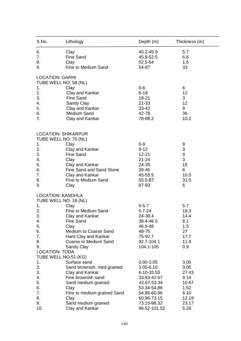
viii
S.No. Lithology Depth (m) Thickness (m) 6. Clay 40.2-45.9 5.7 7. Fine Sand 45.9-52.5 6.6 8. Clay 52.5-54 1.5 9. Fine to Medium Sand 54-87 33 LOCATION: GARHI TUBE WELL NO: 58 (NL) 1. Clay 0-6 6 2. Clay and Kankar 6-18 12 3. Fine Sand 18-21 3 4. Sandy Clay 21-33 12 5. Clay and Kankar 33-42 9 6. Medium Sand 42-78 36 7. Clay and Kankar 78-88.2 10.2 LOCATION: SHIKARPUR TUBE WELL NO: 70 (NL) 1. Clay 0-9 9 2. Clay and Kankar 9-12 3 3. Fine Sand 12-21 9 4. Clay 21-24 3 5. Clay and Kankar 24-39 15 6. Fine Sand and Sand Stone 39-45 6 7. Clay and Kankar 45-55.5 10.5 8. Fine to Medium Sand 55.5-87 31.5 9. Clay 87-93 6 LOCATION: KANDHLA TUBE WELL NO: 18 (NL) 1. Clay 0-5.7 5.7 2. Fine to Medium Sand 5.7-24 18.3 3. Clay and Kankar 24-38.4 14.4 4. Fine Sand 38.4-46.5 8.1 5. Clay 46.5-48 1.5 6. Medium to Coarse Sand 48-75 27 7. Hard Clay and Kankar 75-92.7 17.7 8. Coarse to Medium Sand 92.7-104.1 11.4 9. Sandy Clay 104.1-105 0.9 LOCATION: TODA TUBE WELL NO.51 (KG) 1. Surface sand 0.00-3.05 3.05 2. Sand brownish, med grained 3.05-6.10 3.05 3. Clay and Kankar 6.10-33.53 27.43 4. Fine brownish sand 33.63-42.67 9.14 5. Sand medium grained 42.67-53.34 10.67 6. Clay 53.34-54.86 1.52 7. Fine to medium grained Sand 54.86-60.96 6.10 8. Clay 60.96-73.15 12.19 9. Sand medium grained 73.15-96.32 23.17 10. Clay and Kankar 96.52-101.52 5.28
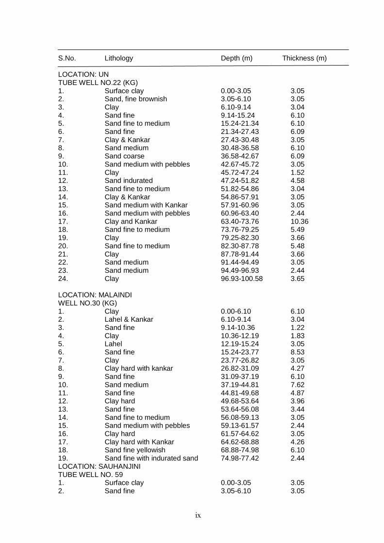
ix
S.No. Lithology Depth (m) Thickness (m) LOCATION: UN TUBE WELL NO.22 (KG) 1. Surface clay 0.00-3.05 3.05 2. Sand, fine brownish 3.05-6.10 3.05 3. Clay 6.10-9.14 3.04 4. Sand fine 9.14-15.24 6.10 5. Sand fine to medium 15.24-21.34 6.10 6. Sand fine 21.34-27.43 6.09 7. Clay & Kankar 27.43-30.48 3.05 8. Sand medium 30.48-36.58 6.10 9. Sand coarse 36.58-42.67 6.09 10. Sand medium with pebbles 42.67-45.72 3.05 11. Clay 45.72-47.24 1.52 12. Sand indurated 47.24-51.82 4.58 13. Sand fine to medium 51.82-54.86 3.04 14. Clay & Kankar 54.86-57.91 3.05 15. Sand medium with Kankar 57.91-60.96 3.05 16. Sand medium with pebbles 60.96-63.40 2.44 17. Clay and Kankar 63.40-73.76 10.36 18. Sand fine to medium 73.76-79.25 5.49 19. Clay 79.25-82.30 3.66 20. Sand fine to medium 82.30-87.78 5.48 21. Clay 87.78-91.44 3.66 22. Sand medium 91.44-94.49 3.05 23. Sand medium 94.49-96.93 2.44 24. Clay 96.93-100.58 3.65 LOCATION: MALAINDI WELL NO.30 (KG) 1. Clay 0.00-6.10 6.10 2. Lahel & Kankar 6.10-9.14 3.04 3. Sand fine 9.14-10.36 1.22 4. Clay 10.36-12.19 1.83 5. Lahel 12.19-15.24 3.05 6. Sand fine 15.24-23.77 8.53 7. Clay 23.77-26.82 3.05 8. Clay hard with kankar 26.82-31.09 4.27 9. Sand fine 31.09-37.19 6.10 10. Sand medium 37.19-44.81 7.62 11. Sand fine 44.81-49.68 4.87 12. Clay hard 49.68-53.64 3.96 13. Sand fine 53.64-56.08 3.44 14. Sand fine to medium 56.08-59.13 3.05 15. Sand medium with pebbles 59.13-61.57 2.44 16. Clay hard 61.57-64.62 3.05 17. Clay hard with Kankar 64.62-68.88 4.26 18. Sand fine yellowish 68.88-74.98 6.10 19. Sand fine with indurated sand 74.98-77.42 2.44 LOCATION: SAUHANJINI TUBE WELL NO. 59 1. Surface clay 0.00-3.05 3.05 2. Sand fine 3.05-6.10 3.05
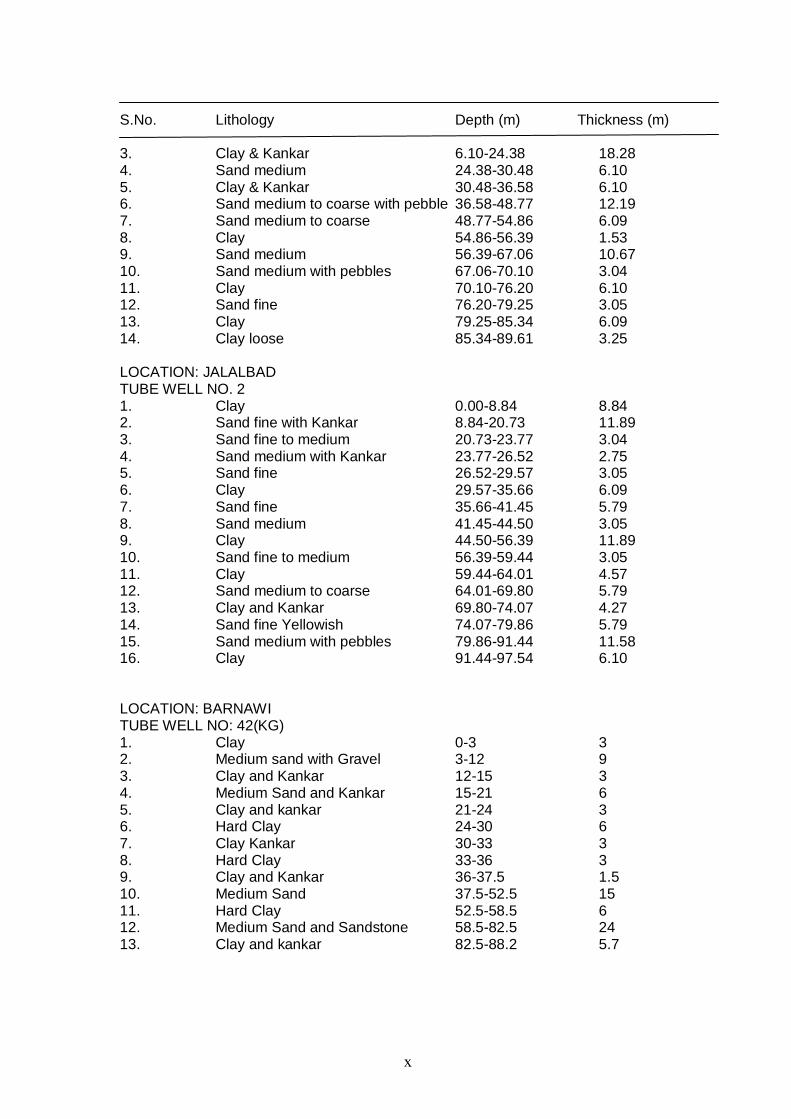
x
S.No. Lithology Depth (m) Thickness (m) 3. Clay & Kankar 6.10-24.38 18.28 4. Sand medium 24.38-30.48 6.10 5. Clay & Kankar 30.48-36.58 6.10 6. Sand medium to coarse with pebble 36.58-48.77 12.19 7. Sand medium to coarse 48.77-54.86 6.09 8. Clay 54.86-56.39 1.53 9. Sand medium 56.39-67.06 10.67 10. Sand medium with pebbles 67.06-70.10 3.04 11. Clay 70.10-76.20 6.10 12. Sand fine 76.20-79.25 3.05 13. Clay 79.25-85.34 6.09 14. Clay loose 85.34-89.61 3.25 LOCATION: JALALBAD TUBE WELL NO. 2 1. Clay 0.00-8.84 8.84 2. Sand fine with Kankar 8.84-20.73 11.89 3. Sand fine to medium 20.73-23.77 3.04 4. Sand medium with Kankar 23.77-26.52 2.75 5. Sand fine 26.52-29.57 3.05 6. Clay 29.57-35.66 6.09 7. Sand fine 35.66-41.45 5.79 8. Sand medium 41.45-44.50 3.05 9. Clay 44.50-56.39 11.89 10. Sand fine to medium 56.39-59.44 3.05 11. Clay 59.44-64.01 4.57 12. Sand medium to coarse 64.01-69.80 5.79 13. Clay and Kankar 69.80-74.07 4.27 14. Sand fine Yellowish 74.07-79.86 5.79 15. Sand medium with pebbles 79.86-91.44 11.58 16. Clay 91.44-97.54 6.10 LOCATION: BARNAWI TUBE WELL NO: 42(KG) 1. Clay 0-3 3 2. Medium sand with Gravel 3-12 9 3. Clay and Kankar 12-15 3 4. Medium Sand and Kankar 15-21 6 5. Clay and kankar 21-24 3 6. Hard Clay 24-30 6 7. Clay Kankar 30-33 3 8. Hard Clay 33-36 3 9. Clay and Kankar 36-37.5 1.5 10. Medium Sand 37.5-52.5 15 11. Hard Clay 52.5-58.5 6 12. Medium Sand and Sandstone 58.5-82.5 24 13. Clay and kankar 82.5-88.2 5.7
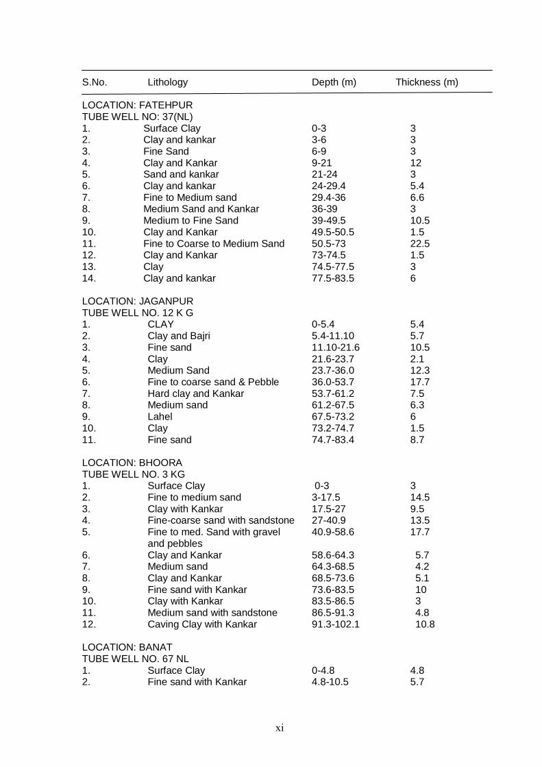
xi
S.No. Lithology Depth (m) Thickness (m) LOCATION: FATEHPUR TUBE WELL NO: 37(NL) 1. Surface Clay 0-3 3 2. Clay and kankar 3-6 3 3. Fine Sand 6-9 3 4. Clay and Kankar 9-21 12 5. Sand and kankar 21-24 3 6. Clay and kankar 24-29.4 5.4 7. Fine to Medium sand 29.4-36 6.6 8. Medium Sand and Kankar 36-39 3 9. Medium to Fine Sand 39-49.5 10.5 10. Clay and Kankar 49.5-50.5 1.5 11. Fine to Coarse to Medium Sand 50.5-73 22.5 12. Clay and Kankar 73-74.5 1.5 13. Clay 74.5-77.5 3 14. Clay and kankar 77.5-83.5 6 LOCATION: JAGANPUR TUBE WELL NO. 12 K G 1. CLAY 0-5.4 5.4 2. Clay and Bajri 5.4-11.10 5.7 3. Fine sand 11.10-21.6 10.5 4. Clay 21.6-23.7 2.1 5. Medium Sand 23.7-36.0 12.3 6. Fine to coarse sand & Pebble 36.0-53.7 17.7 7. Hard clay and Kankar 53.7-61.2 7.5 8. Medium sand 61.2-67.5 6.3 9. Lahel 67.5-73.2 6 10. Clay 73.2-74.7 1.5 11. Fine sand 74.7-83.4 8.7 LOCATION: BHOORA TUBE WELL NO. 3 KG 1. Surface Clay 0-3 3 2. Fine to medium sand 3-17.5 14.5 3. Clay with Kankar 17.5-27 9.5 4. Fine-coarse sand with sandstone 27-40.9 13.5 5. Fine to med. Sand with gravel 40.9-58.6 17.7 and pebbles 6. Clay and Kankar 58.6-64.3 5.7 7. Medium sand 64.3-68.5 4.2 8. Clay and Kankar 68.5-73.6 5.1 9. Fine sand with Kankar 73.6-83.5 10 10. Clay with Kankar 83.5-86.5 3 11. Medium sand with sandstone 86.5-91.3 4.8 12. Caving Clay with Kankar 91.3-102.1 10.8 LOCATION: BANAT TUBE WELL NO. 67 NL 1. Surface Clay 0-4.8 4.8 2. Fine sand with Kankar 4.8-10.5 5.7
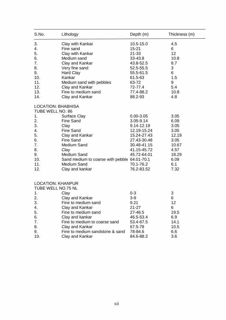
xii
S.No. Lithology Depth (m) Thickness (m) 3. Clay with Kankar 10.5-15.0 4.5 4. Fine sand 15-21 6 5. Clay with Kankar 21-33 12 6. Medium sand 33-43.8 10.8 7. Clay and Kankar 43.8-52.5 8.7 8. Very fine sand 52.5-55.5 3 9. Hard Clay 55.5-61.5 6 10. Kankar 61.5-63 1.5 11. Medium sand with pebbles 63-72 9 12. Clay and Kankar 72-77.4 5.4 13. Fine to medium sand 77.4-88.2 10.8 14. Clay and Kankar 88.2-93 4.8 LOCATION: BHABHISA TUBE WELL NO. 86 1. Surface Clay 0.00-3.05 3.05 2. Fine Sand 3.05-9.14 6.09 3. Clay 9.14-12.19 3.05 4. Fine Sand 12.19-15.24 3.05 5. Clay and Kankar 15.24-27.43 12.19 6. Fine Sand 27.43-30.48 3.05 7. Medium Sand 30.48-41.15 10.67 8. Clay 41.15-45.72 4.57 9. Medium Sand 45.72-64.01 18.29 10. Sand medium to coarse with pebble 64.01-70.1 6.09 11. Medium Sand 70.1-76.2 6.1 12. Clay and kankar 76.2-83.52 7.32
LOCATION: KHANPUR TUBE WELL NO.75 NL 1. Clay 0-3 3 2. Clay and Kankar 3-9 6 3. Fine to medium sand 9.21 12 4. Clay and Kankar 21-27 6 5. Fine to medium sand 27-46.5 19.5 6. Clay and kankar 46.5-53.4 6.9 7. Fine to medium to coarse sand 53.4-67.5 14.1 8. Clay and Kankar 67.5-78 10.5 9. Fine to medium sandstone & sand 78-84.6 6.6 10. Clay and Kankar 84.6-88.2 3.6
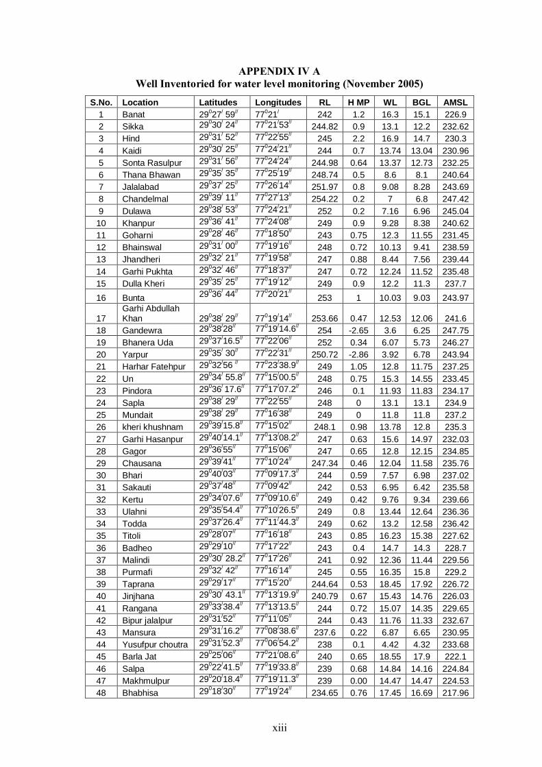
xiii
APPENDIX IV A Well Inventoried for water level monitoring (November 2005)
S.No. Location Latitudes Longitudes RL H MP WL BGL AMSL
1 Banat 29027
/ 59
// 77
021
/ 242 1.2 16.3 15.1 226.9
2 Sikka 29030
/ 24
// 77021
/53
// 244.82 0.9 13.1 12.2 232.62
3 Hind 29031
/ 52
// 77022
/55
// 245 2.2 16.9 14.7 230.3
4 Kaidi 29030
/ 25
// 77024
/21
// 244 0.7 13.74 13.04 230.96
5 Sonta Rasulpur 29031
/ 56
// 77024
/24
// 244.98 0.64 13.37 12.73 232.25
6 Thana Bhawan 29035
/ 35
// 77025
/19
// 248.74 0.5 8.6 8.1 240.64
7 Jalalabad 29037
/ 25
// 77026
/14
// 251.97 0.8 9.08 8.28 243.69
8 Chandelmal 29039
/ 11
// 77027
/13
// 254.22 0.2 7 6.8 247.42
9 Dulawa 29038
/ 53
// 77024
/21
// 252 0.2 7.16 6.96 245.04
10 Khanpur 29036
/ 41
// 77024
/08
// 249 0.9 9.28 8.38 240.62
11 Goharni 29028
/ 46
// 77018
/50
// 243 0.75 12.3 11.55 231.45
12 Bhainswal 29031
/ 00
// 77019
/16
// 248 0.72 10.13 9.41 238.59
13 Jhandheri 29032
/ 21
// 77019
/58
// 247 0.88 8.44 7.56 239.44
14 Garhi Pukhta 29032
/ 46
// 77018
/37
// 247 0.72 12.24 11.52 235.48
15 Dulla Kheri 29035
/ 25
// 77019
/12
// 249 0.9 12.2 11.3 237.7
16 Bunta 29036
/ 44
// 77020
/21
// 253 1 10.03 9.03 243.97
17 Garhi Abdullah Khan
29
038
/ 29
// 77
019
/14
// 253.66 0.47 12.53 12.06 241.6
18 Gandewra 29038
/28
// 77019
/14.6
// 254 -2.65 3.6 6.25 247.75
19 Bhanera Uda 29037
/16.5
// 77022
/06
// 252 0.34 6.07 5.73 246.27
20 Yarpur 29035
/ 30
// 77022
/31
// 250.72 -2.86 3.92 6.78 243.94
21 Harhar Fatehpur 29032
/56
// 77023
/38.9
// 249 1.05 12.8 11.75 237.25
22 Un 29034
/ 55.8
// 77015
/00.5
// 248 0.75 15.3 14.55 233.45
23 Pindora 29036
/ 17.6
// 77017
/07.2
// 246 0.1 11.93 11.83 234.17
24 Sapla 29038
/ 29
// 77022
/55
// 248 0 13.1 13.1 234.9
25 Mundait 29038
/ 29
// 77016
/38
// 249 0 11.8 11.8 237.2
26 kheri khushnam 29039
/15.8
// 77015
/02
// 248.1 0.98 13.78 12.8 235.3
27 Garhi Hasanpur 29040
/14.1
// 77013
/08.2
// 247 0.63 15.6 14.97 232.03
28 Gagor 29036
/55
// 77015
/06
// 247 0.65 12.8 12.15 234.85
29 Chausana 29039
/41
// 77010
/24
// 247.34 0.46 12.04 11.58 235.76
30 Bhari 29040
/03
// 77009
/17.3
// 244 0.59 7.57 6.98 237.02
31 Sakauti 29037
/48
// 77009
/42
// 242 0.53 6.95 6.42 235.58
32 Kertu 29034
/07.6
// 77009
/10.6
// 249 0.42 9.76 9.34 239.66
33 Ulahni 29035
/54.4
// 77010
/26.5
// 249 0.8 13.44 12.64 236.36
34 Todda 29037
/26.4
// 77011
/44.3
// 249 0.62 13.2 12.58 236.42
35 Titoli 29028
/07
// 77016
/18
// 243 0.85 16.23 15.38 227.62
36 Badheo 29029
/10
// 77017
/22
// 243 0.4 14.7 14.3 228.7
37 Malindi 29030
/ 28.2
// 77017
/26
// 241 0.92 12.36 11.44 229.56
38 Purmafi 29032
/ 42
// 77016
/14
// 245 0.55 16.35 15.8 229.2
39 Taprana 29029
/17
// 77015
/20
// 244.64 0.53 18.45 17.92 226.72
40 Jinjhana 29030
/ 43.1
// 77013
/19.9
// 240.79 0.67 15.43 14.76 226.03
41 Rangana 29033
/38.4
// 77013
/13.5
// 244 0.72 15.07 14.35 229.65
42 Bipur jalalpur 29031
/52
// 77011
/05
// 244 0.43 11.76 11.33 232.67
43 Mansura 29031
/16.2
// 77008
/38.6
// 237.6 0.22 6.87 6.65 230.95
44 Yusufpur choutra 29031
/52.3
// 77006
/54.2
// 238 0.1 4.42 4.32 233.68
45 Barla Jat 29025
/06
// 77021
/08.6
// 240 0.65 18.55 17.9 222.1
46 Salpa 29022
/41.5
// 77019
/33.8
// 239 0.68 14.84 14.16 224.84
47 Makhmulpur 29020
/18.4
// 77019
/11.3
// 239 0.00 14.47 14.47 224.53
48 Bhabhisa 29018
/30
// 77019
/24
// 234.65 0.76 17.45 16.69 217.96
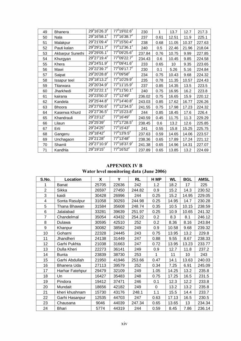
xiv
49 Bhanera 29016
/26.3
// 77019
/02.6
// 230 1 13.7 12.7 217.3
50 Nala 29016
/58.1
// 77016
/38.7
// 237 0.61 12.51 11.9 225.1
51 Malakpur 29021
/09.4
// 77015
/50.4
// 238 0.68 11.05 10.37 227.63
52 Pauti kalan 29029
/11.7
// 77012
/36.1
// 240 0.5 22.46 21.96 218.04
53 Akbarpur Sunethi 29029
/05.1
// 77009
/25.6
// 237.84 0.76 10.75 9.99 227.85
54 Khurgyan 29027
/19.4
// 77009
/22.7
// 234.43 0.6 10.45 9.85 224.58
55 Khera 29024
/51.9
// 77009
/41.6
// 233 0.65 10 9.35 223.65
56 Mawi 29022
/39.7
// 77009
/17.7
// 230 0.1 5.26 5.16 224.84
57 Saipat 29020
/28.8
// 77009
/58
// 234 0.75 10.43 9.68 224.32
58 Issapur teel 29018
/13.2
// 77010
/29.9
// 235 0.78 11.35 10.57 224.43
59 Titarwara 29020
/34.9
// 77011
/15.9
// 237 0.85 14.35 13.5 223.5
60 Jharkhedi 29022
/22.1
// 77011
/50.1
// 240 0.75 16.95 16.2 223.8
61 kairana 29023
/50.3
// 77012
/49
// 236.02 0.75 16.65 15.9 220.12
62 Kandela 29025
/44.8
// 77014
/40.8
// 243.03 0.85 17.62 16.77 226.26
63 Bhoora 29027
/00.6
// 77012
/34.5
// 241.55 0.75 17.98 17.23 224.32
64 Kaserwa Khurd 29027
/36.5
// 77015
/23.8
// 244 0.85 18.45 17.6 226.4
65 Khandrauli 29023
/12
// 77016
/49
// 240.59 0.45 11.75 11.3 229.29
66 Lilaun 29025
/39
// 77017
/28.5
// 238.45 0.6 13.2 12.6 225.85
67 Erti 29024
/25
// 77015
/43
// 241 0.55 15.8 15.25 225.75
68 Gangeru 29018
/42
// 77013
/9.5
// 237.63 0.59 14.65 14.06 223.57
69 Unchagaon 29021
/28
// 77013
/48
// 238.36 0.65 17.89 17.24 221.12
70 Shamli 29027
/10.9
// 77018
/37.9
// 241.38 0.65 14.96 14.31 227.07
71 Kandhla 29019
/15
// 77016
/52
// 237.89 0.65 13.85 13.2 224.69
APPENDIX IV B Water level monitoring data (June 2006)
S.No. Location X Y RL H MP WL BGL AMSL
1 Banat 25705 22636 242 1.2 18.2 17 225
2 Sikka 26597 27450 244.82 0.9 15.2 14.3 230.52
3 kaidi 30428 26996 244 0.25 15.2 14.95 229.05
4 Sonta Rasulpur 31058 30293 244.98 0.25 14.95 14.7 230.28
5 Thana Bhawan 31584 35608 248.74 0.35 10.5 10.15 238.59
6 Jalalabad 33281 39639 251.97 0.25 10.9 10.65 241.32
7 Chandelmal 35054 43432 254.22 0.2 8.3 8.1 246.12
8 Dulawa 30595 42510 252 0.2 8.36 8.16 243.84
9 Khanpur 30082 38562 249 0.9 10.58 9.68 239.32
10 Goharni 22328 24445 243 0.75 13.95 13.2 229.8
11 Jhandheri 24138 31449 247 0.88 9.55 8.67 238.33
12 Garhi Pukhta 21038 31663 247 0.72 13.95 13.23 233.77
13 Dulla Kheri 22273 36141 249 0.9 12.7 11.8 237.2
14 Bunta 23839 38730 253 1 11 10 243
15 Garhi Abdullah 21950 41946 253.66 0.47 14.1 13.63 240.03
16 Bhanera Uda 27113 39579 252 0.34 7.25 6.91 245.09
17 Harhar Fatehpur 29479 32109 249 1.05 14.25 13.2 235.8
18 Un 16427 35483 248 0.75 17.25 16.5 231.5
19 Pindora 19412 37471 246 0.1 12.3 12.2 233.8
20 Mundait 18656 42182 249 0 13.2 13.2 235.8
21 kheri khushnam 15730 43176 248.1 1.1 15.5 14.4 233.7
22 Garhi Hasanpur 12535 44703 247 0.63 17.13 16.5 230.5
23 Chausana 9046 44039 247.34 0.65 13.65 13 234.34
24 Bhari 5774 44319 244 0.59 8.45 7.86 236.14
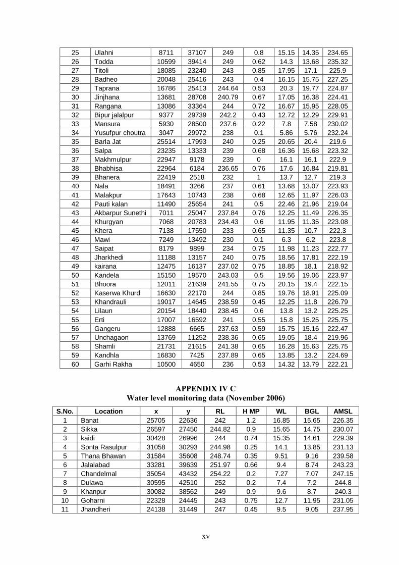
xv
25 Ulahni 8711 37107 249 0.8 15.15 14.35 234.65
26 Todda 10599 39414 249 0.62 14.3 13.68 235.32
27 Titoli 18085 23240 243 0.85 17.95 17.1 225.9
28 Badheo 20048 25416 243 0.4 16.15 15.75 227.25
29 Taprana 16786 25413 244.64 0.53 20.3 19.77 224.87
30 Jinjhana 13681 28708 240.79 0.67 17.05 16.38 224.41
31 Rangana 13086 33364 244 0.72 16.67 15.95 228.05
32 Bipur jalalpur 9377 29739 242.2 0.43 12.72 12.29 229.91
33 Mansura 5930 28500 237.6 0.22 7.8 7.58 230.02
34 Yusufpur choutra 3047 29972 238 0.1 5.86 5.76 232.24
35 Barla Jat 25514 17993 240 0.25 20.65 20.4 219.6
36 Salpa 23235 13333 239 0.68 16.36 15.68 223.32
37 Makhmulpur 22947 9178 239 0 16.1 16.1 222.9
38 Bhabhisa 22964 6184 236.65 0.76 17.6 16.84 219.81
39 Bhanera 22419 2518 232 1 13.7 12.7 219.3
40 Nala 18491 3266 237 0.61 13.68 13.07 223.93
41 Malakpur 17643 10743 238 0.68 12.65 11.97 226.03
42 Pauti kalan 11490 25654 241 0.5 22.46 21.96 219.04
43 Akbarpur Sunethi 7011 25047 237.84 0.76 12.25 11.49 226.35
44 Khurgyan 7068 20783 234.43 0.6 11.95 11.35 223.08
45 Khera 7138 17550 233 0.65 11.35 10.7 222.3
46 Mawi 7249 13492 230 0.1 6.3 6.2 223.8
47 Saipat 8179 9899 234 0.75 11.98 11.23 222.77
48 Jharkhedi 11188 13157 240 0.75 18.56 17.81 222.19
49 kairana 12475 16137 237.02 0.75 18.85 18.1 218.92
50 Kandela 15150 19570 243.03 0.5 19.56 19.06 223.97
51 Bhoora 12011 21639 241.55 0.75 20.15 19.4 222.15
52 Kaserwa Khurd 16630 22170 244 0.85 19.76 18.91 225.09
53 Khandrauli 19017 14645 238.59 0.45 12.25 11.8 226.79
54 Lilaun 20154 18440 238.45 0.6 13.8 13.2 225.25
55 Erti 17007 16592 241 0.55 15.8 15.25 225.75
56 Gangeru 12888 6665 237.63 0.59 15.75 15.16 222.47
57 Unchagaon 13769 11252 238.36 0.65 19.05 18.4 219.96
58 Shamli 21731 21615 241.38 0.65 16.28 15.63 225.75
59 Kandhla 16830 7425 237.89 0.65 13.85 13.2 224.69
60 Garhi Rakha 10500 4650 236 0.53 14.32 13.79 222.21
APPENDIX IV C Water level monitoring data (November 2006)
S.No. Location x y RL H MP WL BGL AMSL
1 Banat 25705 22636 242 1.2 16.85 15.65 226.35
2 Sikka 26597 27450 244.82 0.9 15.65 14.75 230.07
3 kaidi 30428 26996 244 0.74 15.35 14.61 229.39
4 Sonta Rasulpur 31058 30293 244.98 0.25 14.1 13.85 231.13
5 Thana Bhawan 31584 35608 248.74 0.35 9.51 9.16 239.58
6 Jalalabad 33281 39639 251.97 0.66 9.4 8.74 243.23
7 Chandelmal 35054 43432 254.22 0.2 7.27 7.07 247.15
8 Dulawa 30595 42510 252 0.2 7.4 7.2 244.8
9 Khanpur 30082 38562 249 0.9 9.6 8.7 240.3
10 Goharni 22328 24445 243 0.75 12.7 11.95 231.05
11 Jhandheri 24138 31449 247 0.45 9.5 9.05 237.95
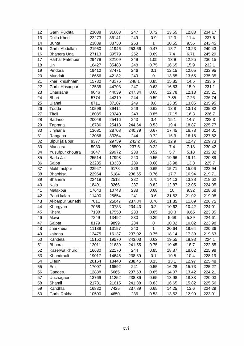
xvi
12 Garhi Pukhta 21038 31663 247 0.72 13.55 12.83 234.17
13 Dulla Kheri 22273 36141 249 0.9 12.3 11.4 237.6
14 Bunta 23839 38730 253 1 10.55 9.55 243.45
15 Garhi Abdullah 21950 41946 253.66 0.47 13.7 13.23 240.43
16 Bhanera Uda 27113 39579 252 0.69 7.4 6.71 245.29
17 Harhar Fatehpur 29479 32109 249 1.05 13.9 12.85 236.15
18 Un 16427 35483 248 0.75 16.65 15.9 232.1
19 Pindora 19412 37471 246 0.1 12.15 12.05 233.95
20 Mundait 18656 42182 249 0 13.65 13.65 235.35
21 kheri khushnam 15730 43176 248.1 0.85 15.35 14.5 233.6
22 Garhi Hasanpur 12535 44703 247 0.63 16.53 15.9 231.1
23 Chausana 9046 44039 247.34 0.65 12.78 12.13 235.21
24 Bhari 5774 44319 244 0.59 7.85 7.26 236.74
25 Ulahni 8711 37107 249 0.8 13.85 13.05 235.95
26 Todda 10599 39414 249 0.62 13.8 13.18 235.82
27 Titoli 18085 23240 243 0.85 17.15 16.3 226.7
28 Badheo 20048 25416 243 0.4 15.1 14.7 228.3
29 Taprana 16786 25413 244.64 0.53 19.4 18.87 225.77
30 Jinjhana 13681 28708 240.79 0.67 17.45 16.78 224.01
31 Rangana 13086 33364 244 0.72 16.9 16.18 227.82
32 Bipur jalalpur 9377 29739 242.2 0.43 12.9 12.47 229.73
33 Mansura 5930 28500 237.6 0.22 7.4 7.18 230.42
34 Yusufpur choutra 3047 29972 238 0.52 5.7 5.18 232.82
35 Barla Jat 25514 17993 240 0.55 19.66 19.11 220.89
36 Salpa 23235 13333 239 0.68 13.98 13.3 225.7
37 Makhmulpur 22947 9178 239 0.65 15.71 15.06 223.94
38 Bhabhisa 22964 6184 236.65 0.76 17.7 16.94 219.71
39 Bhanera 22419 2518 232 0.75 14.13 13.38 218.62
40 Nala 18491 3266 237 0.82 12.87 12.05 224.95
41 Malakpur 17643 10743 238 0.68 10 9.32 228.68
42 Pauti kalan 11490 25654 241 0.6 21.62 21.02 219.98
43 Akbarpur Sunethi 7011 25047 237.84 0.76 11.85 11.09 226.75
44 Khurgyan 7068 20783 234.43 0.2 10.62 10.42 224.01
45 Khera 7138 17550 233 0.65 10.3 9.65 223.35
46 Mawi 7249 13492 230 0.29 5.68 5.39 224.61
47 Saipat 8179 9899 234 0 10.02 10.02 223.98
48 Jharkhedi 11188 13157 240 1 20.64 19.64 220.36
49 kairana 12475 16137 237.02 0.75 18.14 17.39 219.63
50 Kandela 15150 19570 243.03 0.62 19.55 18.93 224.1
51 Bhoora 12011 21639 241.55 0.75 19.45 18.7 222.85
52 Kaserwa Khurd 16630 22170 244 0.85 18.87 18.02 225.98
53 Khandrauli 19017 14645 238.59 0.1 10.5 10.4 228.19
54 Lilaun 20154 18440 238.45 0.13 13.1 12.97 225.48
55 Erti 17007 16592 241 0.55 16.28 15.73 225.27
56 Gangeru 12888 6665 237.63 0.65 14.07 13.42 224.21
57 Unchagaon 13769 11252 238.36 0.65 18.98 18.33 220.03
58 Shamli 21731 21615 241.38 0.83 16.65 15.82 225.56
59 Kandhla 16830 7425 237.89 0.65 14.25 13.6 224.29
60 Garhi Rakha 10500 4650 236 0.53 13.52 12.99 223.01
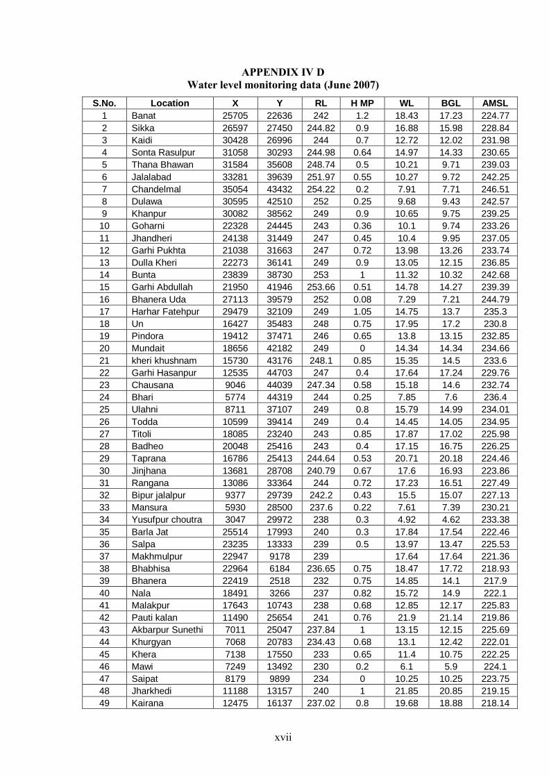
xvii
APPENDIX IV D Water level monitoring data (June 2007)
S.No. Location X Y RL H MP WL BGL AMSL
1 Banat 25705 22636 242 1.2 18.43 17.23 224.77
2 Sikka 26597 27450 244.82 0.9 16.88 15.98 228.84
3 Kaidi 30428 26996 244 0.7 12.72 12.02 231.98
4 Sonta Rasulpur 31058 30293 244.98 0.64 14.97 14.33 230.65
5 Thana Bhawan 31584 35608 248.74 0.5 10.21 9.71 239.03
6 Jalalabad 33281 39639 251.97 0.55 10.27 9.72 242.25
7 Chandelmal 35054 43432 254.22 0.2 7.91 7.71 246.51
8 Dulawa 30595 42510 252 0.25 9.68 9.43 242.57
9 Khanpur 30082 38562 249 0.9 10.65 9.75 239.25
10 Goharni 22328 24445 243 0.36 10.1 9.74 233.26
11 Jhandheri 24138 31449 247 0.45 10.4 9.95 237.05
12 Garhi Pukhta 21038 31663 247 0.72 13.98 13.26 233.74
13 Dulla Kheri 22273 36141 249 0.9 13.05 12.15 236.85
14 Bunta 23839 38730 253 1 11.32 10.32 242.68
15 Garhi Abdullah 21950 41946 253.66 0.51 14.78 14.27 239.39
16 Bhanera Uda 27113 39579 252 0.08 7.29 7.21 244.79
17 Harhar Fatehpur 29479 32109 249 1.05 14.75 13.7 235.3
18 Un 16427 35483 248 0.75 17.95 17.2 230.8
19 Pindora 19412 37471 246 0.65 13.8 13.15 232.85
20 Mundait 18656 42182 249 0 14.34 14.34 234.66
21 kheri khushnam 15730 43176 248.1 0.85 15.35 14.5 233.6
22 Garhi Hasanpur 12535 44703 247 0.4 17.64 17.24 229.76
23 Chausana 9046 44039 247.34 0.58 15.18 14.6 232.74
24 Bhari 5774 44319 244 0.25 7.85 7.6 236.4
25 Ulahni 8711 37107 249 0.8 15.79 14.99 234.01
26 Todda 10599 39414 249 0.4 14.45 14.05 234.95
27 Titoli 18085 23240 243 0.85 17.87 17.02 225.98
28 Badheo 20048 25416 243 0.4 17.15 16.75 226.25
29 Taprana 16786 25413 244.64 0.53 20.71 20.18 224.46
30 Jinjhana 13681 28708 240.79 0.67 17.6 16.93 223.86
31 Rangana 13086 33364 244 0.72 17.23 16.51 227.49
32 Bipur jalalpur 9377 29739 242.2 0.43 15.5 15.07 227.13
33 Mansura 5930 28500 237.6 0.22 7.61 7.39 230.21
34 Yusufpur choutra 3047 29972 238 0.3 4.92 4.62 233.38
35 Barla Jat 25514 17993 240 0.3 17.84 17.54 222.46
36 Salpa 23235 13333 239 0.5 13.97 13.47 225.53
37 Makhmulpur 22947 9178 239 17.64 17.64 221.36
38 Bhabhisa 22964 6184 236.65 0.75 18.47 17.72 218.93
39 Bhanera 22419 2518 232 0.75 14.85 14.1 217.9
40 Nala 18491 3266 237 0.82 15.72 14.9 222.1
41 Malakpur 17643 10743 238 0.68 12.85 12.17 225.83
42 Pauti kalan 11490 25654 241 0.76 21.9 21.14 219.86
43 Akbarpur Sunethi 7011 25047 237.84 1 13.15 12.15 225.69
44 Khurgyan 7068 20783 234.43 0.68 13.1 12.42 222.01
45 Khera 7138 17550 233 0.65 11.4 10.75 222.25
46 Mawi 7249 13492 230 0.2 6.1 5.9 224.1
47 Saipat 8179 9899 234 0 10.25 10.25 223.75
48 Jharkhedi 11188 13157 240 1 21.85 20.85 219.15
49 Kairana 12475 16137 237.02 0.8 19.68 18.88 218.14

xviii
50 Kandela 15150 19570 243.03 0.62 19.84 19.22 223.81
51 Bhoora 12011 21639 241.55 0.8 20.33 19.53 222.02
52 Kaserwa Khurd 16630 22170 244 0.85 19.15 18.3 225.7
53 Khandrauli 19017 14645 238.59 0.12 12.6 12.48 226.11
54 Lilaun 20154 18440 238.45 1 15.9 14.9 223.55
55 Erti 17007 16592 241 0.45 17 16.55 224.45
56 Gangeru 12888 6665 237.63 0.6 15.28 14.68 222.95
57 Unchagaon 13769 11252 238.36 0.65 19.75 19.1 219.26
58 Shamli 21731 21615 241.38 0.65 17.65 17 224.38
59 Kandhla 16830 7425 237.89 0.7 15.4 14.7 223.19
60 Garhi Rakha 10500 4650 236 0.5 14.85 14.35 221.65
APPENDIX IV E Water level monitoring data (November 2007)
S.No. Location X Y RL H MP WL BGL AMSL
1 Banat 25705 22636 242 1.2 19.62 18.42 223.58
2 Sikka 26597 27450 244.82 0.9 17 16.1 228.72
3 Kaidi 30428 26996 244 0.7 15.73 15.03 228.97
4 Sonta Rasulpur 31058 30293 244.98 0.64 15.57 14.93 230.05
5 Thana Bhawan 31584 35608 248.74 0.5 10.55 10.05 238.69
6 Jalalabad 33281 39639 251.97 0.55 10.42 9.87 242.1
7 Chandelmal 35054 43432 254.22 0.2 7.95 7.75 246.47
8 Dulawa 30595 42510 252 0.9 9.94 9.04 242.96
9 Khanpur 30082 38562 249 0.9 10.82 9.92 239.08
10 Goharni 22328 24445 243 0.93 11.2 10.27 232.73
11 Jhandheri 24138 31449 247 0.45 10.74 10.29 236.71
12 Garhi Pukhta 21038 31663 247 0.72 13.57 12.85 234.15
13 Dulla Kheri 22273 36141 249 0.82 13.02 12.2 236.8
14 Bunta 23839 38730 253 0.9 11.3 10.4 242.6
15 Garhi Abdullah 21950 41946 253.66 0.51 15.12 14.61 239.05
16 Bhanera Uda 27113 39579 252 0.08 6.95 6.87 245.13
17 Harhar Fatehpur 29479 32109 249 1.05 15.11 14.06 234.94
18 Un 16427 35483 248 0.75 19.94 19.19 228.81
19 Pindora 19412 37471 246 0.65 13.7 13.05 232.95
20 Mundait 18656 42182 249 0 14.3 14.3 234.7
21 kheri khushnam 15730 43176 248.1 0.6 15.15 14.55 233.55
22 Garhi Hasanpur 12535 44703 247 0.4 17.29 16.89 230.11
23 Chausana 9046 44039 247.34 0.58 15.37 14.79 232.55
24 Bhari 5774 44319 244 0.25 8.21 7.96 236.04
25 Ulahni 8711 37107 249 0.8 16.39 15.59 233.41
26 Todda 10599 39414 249 0.4 12.33 11.93 237.07
27 Titoli 18085 23240 243 0.85 18.34 17.49 225.51
28 Badheo 20048 25416 243 0.4 17.14 16.74 226.26
29 Taprana 16786 25413 244.64 0.68 18.78 18.1 226.54
30 Jinjhana 13681 28708 240.79 0.65 18.12 17.47 223.32
31 Rangana 13086 33364 244 0.7 18.68 17.98 226.02
32 Bipur jalalpur 9377 29739 242.2 0.52 13.65 13.13 229.07
33 Mansura 5930 28500 237.6 0.22 7.41 7.19 230.41
34 Yusufpur choutra 3047 29972 238 0.3 5.2 4.9 233.1
35 Barla Jat 25514 17993 240 0.3 18.89 18.59 221.41
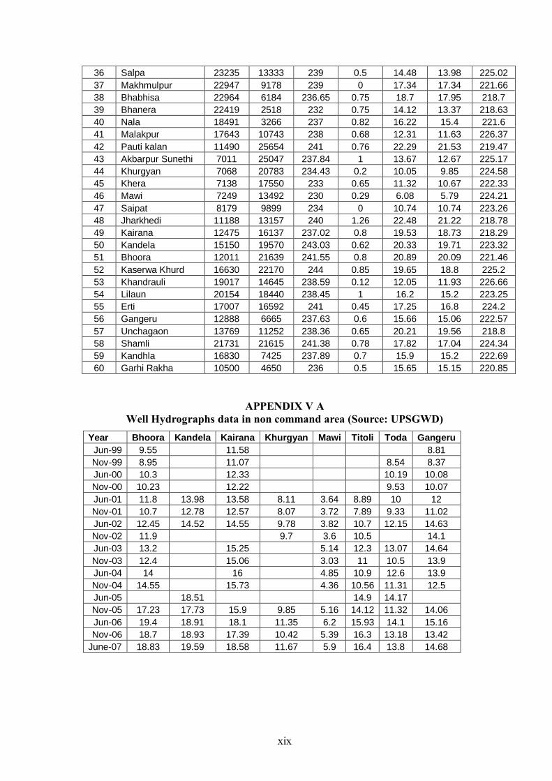
xix
36 Salpa 23235 13333 239 0.5 14.48 13.98 225.02
37 Makhmulpur 22947 9178 239 0 17.34 17.34 221.66
38 Bhabhisa 22964 6184 236.65 0.75 18.7 17.95 218.7
39 Bhanera 22419 2518 232 0.75 14.12 13.37 218.63
40 Nala 18491 3266 237 0.82 16.22 15.4 221.6
41 Malakpur 17643 10743 238 0.68 12.31 11.63 226.37
42 Pauti kalan 11490 25654 241 0.76 22.29 21.53 219.47
43 Akbarpur Sunethi 7011 25047 237.84 1 13.67 12.67 225.17
44 Khurgyan 7068 20783 234.43 0.2 10.05 9.85 224.58
45 Khera 7138 17550 233 0.65 11.32 10.67 222.33
46 Mawi 7249 13492 230 0.29 6.08 5.79 224.21
47 Saipat 8179 9899 234 0 10.74 10.74 223.26
48 Jharkhedi 11188 13157 240 1.26 22.48 21.22 218.78
49 Kairana 12475 16137 237.02 0.8 19.53 18.73 218.29
50 Kandela 15150 19570 243.03 0.62 20.33 19.71 223.32
51 Bhoora 12011 21639 241.55 0.8 20.89 20.09 221.46
52 Kaserwa Khurd 16630 22170 244 0.85 19.65 18.8 225.2
53 Khandrauli 19017 14645 238.59 0.12 12.05 11.93 226.66
54 Lilaun 20154 18440 238.45 1 16.2 15.2 223.25
55 Erti 17007 16592 241 0.45 17.25 16.8 224.2
56 Gangeru 12888 6665 237.63 0.6 15.66 15.06 222.57
57 Unchagaon 13769 11252 238.36 0.65 20.21 19.56 218.8
58 Shamli 21731 21615 241.38 0.78 17.82 17.04 224.34
59 Kandhla 16830 7425 237.89 0.7 15.9 15.2 222.69
60 Garhi Rakha 10500 4650 236 0.5 15.65 15.15 220.85
APPENDIX V A Well Hydrographs data in non command area (Source: UPSGWD)
Year Bhoora Kandela Kairana Khurgyan Mawi Titoli Toda Gangeru
Jun-99 9.55 11.58 8.81
Nov-99 8.95 11.07 8.54 8.37
Jun-00 10.3 12.33 10.19 10.08
Nov-00 10.23 12.22 9.53 10.07
Jun-01 11.8 13.98 13.58 8.11 3.64 8.89 10 12
Nov-01 10.7 12.78 12.57 8.07 3.72 7.89 9.33 11.02
Jun-02 12.45 14.52 14.55 9.78 3.82 10.7 12.15 14.63
Nov-02 11.9 9.7 3.6 10.5 14.1
Jun-03 13.2 15.25 5.14 12.3 13.07 14.64
Nov-03 12.4 15.06 3.03 11 10.5 13.9
Jun-04 14 16 4.85 10.9 12.6 13.9
Nov-04 14.55 15.73 4.36 10.56 11.31 12.5
Jun-05 18.51 14.9 14.17
Nov-05 17.23 17.73 15.9 9.85 5.16 14.12 11.32 14.06
Jun-06 19.4 18.91 18.1 11.35 6.2 15.93 14.1 15.16
Nov-06 18.7 18.93 17.39 10.42 5.39 16.3 13.18 13.42
June-07 18.83 19.59 18.58 11.67 5.9 16.4 13.8 14.68
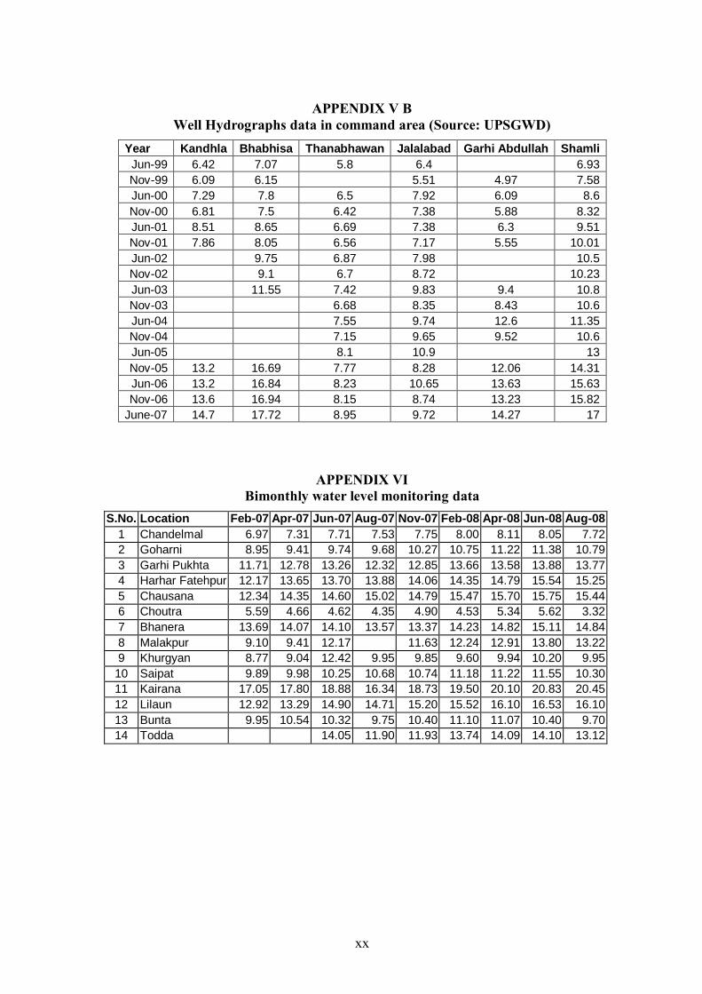
xx
APPENDIX V B
Well Hydrographs data in command area (Source: UPSGWD) Year Kandhla Bhabhisa Thanabhawan Jalalabad Garhi Abdullah Shamli
Jun-99 6.42 7.07 5.8 6.4 6.93
Nov-99 6.09 6.15 5.51 4.97 7.58
Jun-00 7.29 7.8 6.5 7.92 6.09 8.6
Nov-00 6.81 7.5 6.42 7.38 5.88 8.32
Jun-01 8.51 8.65 6.69 7.38 6.3 9.51
Nov-01 7.86 8.05 6.56 7.17 5.55 10.01
Jun-02 9.75 6.87 7.98 10.5
Nov-02 9.1 6.7 8.72 10.23
Jun-03 11.55 7.42 9.83 9.4 10.8
Nov-03 6.68 8.35 8.43 10.6
Jun-04 7.55 9.74 12.6 11.35
Nov-04 7.15 9.65 9.52 10.6
Jun-05 8.1 10.9 13
Nov-05 13.2 16.69 7.77 8.28 12.06 14.31
Jun-06 13.2 16.84 8.23 10.65 13.63 15.63
Nov-06 13.6 16.94 8.15 8.74 13.23 15.82
June-07 14.7 17.72 8.95 9.72 14.27 17
APPENDIX VI Bimonthly water level monitoring data
S.No. Location Feb-07 Apr-07 Jun-07 Aug-07 Nov-07 Feb-08 Apr-08 Jun-08 Aug-08
1 Chandelmal 6.97 7.31 7.71 7.53 7.75 8.00 8.11 8.05 7.72
2 Goharni 8.95 9.41 9.74 9.68 10.27 10.75 11.22 11.38 10.79
3 Garhi Pukhta 11.71 12.78 13.26 12.32 12.85 13.66 13.58 13.88 13.77
4 Harhar Fatehpur 12.17 13.65 13.70 13.88 14.06 14.35 14.79 15.54 15.25
5 Chausana 12.34 14.35 14.60 15.02 14.79 15.47 15.70 15.75 15.44
6 Choutra 5.59 4.66 4.62 4.35 4.90 4.53 5.34 5.62 3.32
7 Bhanera 13.69 14.07 14.10 13.57 13.37 14.23 14.82 15.11 14.84
8 Malakpur 9.10 9.41 12.17 11.63 12.24 12.91 13.80 13.22
9 Khurgyan 8.77 9.04 12.42 9.95 9.85 9.60 9.94 10.20 9.95
10 Saipat 9.89 9.98 10.25 10.68 10.74 11.18 11.22 11.55 10.30
11 Kairana 17.05 17.80 18.88 16.34 18.73 19.50 20.10 20.83 20.45
12 Lilaun 12.92 13.29 14.90 14.71 15.20 15.52 16.10 16.53 16.10
13 Bunta 9.95 10.54 10.32 9.75 10.40 11.10 11.07 10.40 9.70
14 Todda 14.05 11.90 11.93 13.74 14.09 14.10 13.12
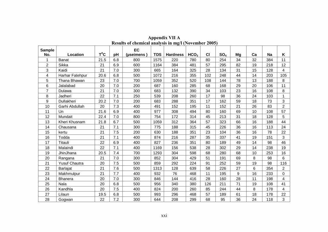
xxi
Appendix VII A Results of chemical analysis in mg/l (November 2005)
Sample No. Location T
0C pH
EC (µseimens ) TDS Hardness HCO3 Cl SO4 Mg Ca Na K
1 Banat 21.5 6.8 800 1575 220 780 80 254 34 32 384 11
2 Sikka 21 6.9 600 1164 384 481 57 295 82 19 218 12
3 Kaidi 21 7.0 300 665 164 325 28 134 31 15 128 4
4 Harhar Fatehpur 20.6 6.8 500 1072 216 355 102 248 44 14 203 105
5 Thana Bhawan 23 7.0 700 1059 352 520 108 144 78 13 188 8
6 Jalalabad 20 7.0 200 687 160 285 68 168 29 20 106 11
7 Dulawa 21 7.0 300 683 132 390 34 103 23 16 108 8
8 Jadheri 22 7.1 250 539 208 260 17 98 36 24 103 1
9 Dullakheri 20.2 7.0 200 683 288 351 17 162 59 18 73 3
10 Garhi Abdullah 20 7.3 400 491 152 195 11 152 21 26 83 2
11 Un 21.6 6.9 400 977 308 494 80 160 69 10 108 57
12 Mundait 22.4 7.0 800 754 172 314 45 213 31 18 128 5
13 Kheri Khusnam 21.8 6.7 500 1059 312 364 57 323 66 16 188 44
14 Chausana 21 7.1 300 775 188 315 45 226 36 16 113 24
15 kertu 21 7.5 200 630 188 351 23 104 36 16 78 22
16 Todda 21 7.1 400 874 216 287 35 337 41 19 151 3
17 Titauli 22 6.9 400 827 236 351 80 189 49 14 98 46
18 Malaindi 22 7.1 400 1169 156 538 28 302 29 14 238 19
19 JhinJhana 20.5 7.4 700 1293 304 598 68 280 68 10 253 16
20 Rangana 21 7.0 300 852 304 429 51 191 69 8 98 6
21 Yusuf Chautra 20 7.5 500 859 292 224 91 252 59 19 98 116
22 Barlajat 21 7.6 500 1313 128 639 58 226 27 6 354 2
23 Makhmulpur 21 7.7 400 932 76 468 11 195 9 16 233 0
24 Bhanera 20 7.0 300 846 144 416 28 160 28 11 198 4
25 Nala 20 6.8 500 956 340 380 126 211 71 19 108 41
26 Kandhla 20 7.5 400 824 200 260 85 244 44 8 178 4
27 Lilaun 19.5 6.8 500 993 296 468 57 189 61 18 178 22
28 Gogwan 22 7.2 300 644 208 299 68 95 36 24 118 3
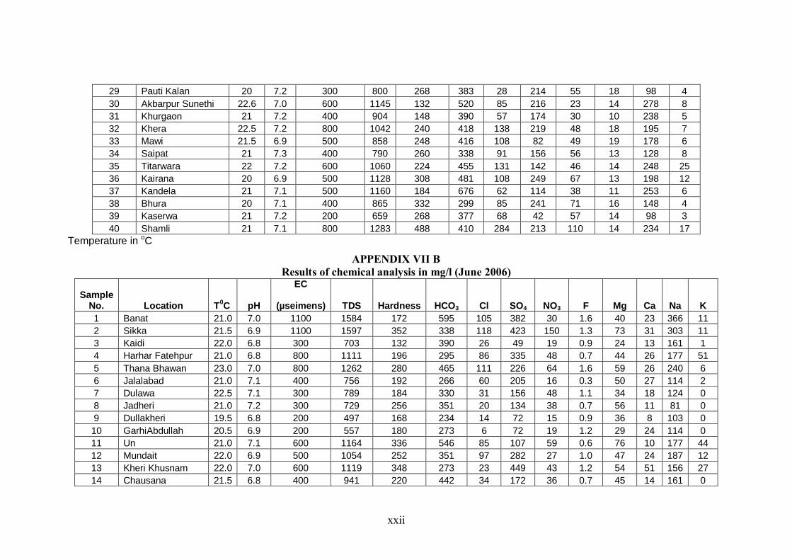
xxii
29 Pauti Kalan 20 7.2 300 800 268 383 28 214 55 18 98 4
30 Akbarpur Sunethi 22.6 7.0 600 1145 132 520 85 216 23 14 278 8
31 Khurgaon 21 7.2 400 904 148 390 57 174 30 10 238 5
32 Khera 22.5 7.2 800 1042 240 418 138 219 48 18 195 7
33 Mawi 21.5 6.9 500 858 248 416 108 82 49 19 178 6
34 Saipat 21 7.3 400 790 260 338 91 156 56 13 128 8
35 Titarwara 22 7.2 600 1060 224 455 131 142 46 14 248 25
36 Kairana 20 6.9 500 1128 308 481 108 249 67 13 198 12
37 Kandela 21 7.1 500 1160 184 676 62 114 38 11 253 6
38 Bhura 20 7.1 400 865 332 299 85 241 71 16 148 4
39 Kaserwa 21 7.2 200 659 268 377 68 42 57 14 98 3
40 Shamli 21 7.1 800 1283 488 410 284 213 110 14 234 17
Temperature in oC
APPENDIX VII B Results of chemical analysis in mg/l (June 2006)
Sample No. Location T
0C pH
EC
(µseimens) TDS Hardness HCO3 Cl SO4 NO3 F Mg Ca Na K
1 Banat 21.0 7.0 1100 1584 172 595 105 382 30 1.6 40 23 366 11
2 Sikka 21.5 6.9 1100 1597 352 338 118 423 150 1.3 73 31 303 11
3 Kaidi 22.0 6.8 300 703 132 390 26 49 19 0.9 24 13 161 1
4 Harhar Fatehpur 21.0 6.8 800 1111 196 295 86 335 48 0.7 44 26 177 51
5 Thana Bhawan 23.0 7.0 800 1262 280 465 111 226 64 1.6 59 26 240 6
6 Jalalabad 21.0 7.1 400 756 192 266 60 205 16 0.3 50 27 114 2
7 Dulawa 22.5 7.1 300 789 184 330 31 156 48 1.1 34 18 124 0
8 Jadheri 21.0 7.2 300 729 256 351 20 134 38 0.7 56 11 81 0
9 Dullakheri 19.5 6.8 200 497 168 234 14 72 15 0.9 36 8 103 0
10 GarhiAbdullah 20.5 6.9 200 557 180 273 6 72 19 1.2 29 24 114 0
11 Un 21.0 7.1 600 1164 336 546 85 107 59 0.6 76 10 177 44
12 Mundait 22.0 6.9 500 1054 252 351 97 282 27 1.0 47 24 187 12
13 Kheri Khusnam 22.0 7.0 600 1119 348 273 23 449 43 1.2 54 51 156 27
14 Chausana 21.5 6.8 400 941 220 442 34 172 36 0.7 45 14 161 0
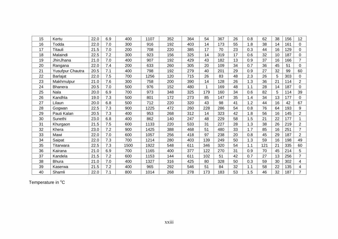
xxiii
15 Kertu 22.0 6.9 400 1107 352 364 54 367 26 0.8 62 38 156 12
16 Todda 22.0 7.0 300 916 192 403 14 173 55 1.8 38 14 161 0
17 Titauli 21.5 7.0 200 708 220 385 17 70 23 0.3 44 16 129 0
18 Malaindi 22.5 7.2 300 923 156 325 14 319 17 0.6 32 10 187 0
19 JhinJhana 21.0 7.0 400 907 192 429 43 182 13 0.9 37 16 166 7
20 Rangana 22.0 7.4 200 633 260 305 20 109 34 0.7 36 45 51 0
21 Yusufpur Chautra 20.5 7.1 400 798 192 279 40 201 29 0.9 27 32 99 60
22 Barlajat 22.0 7.5 700 1256 120 715 26 83 48 2.3 26 5 303 0
23 Makhmulpur 21.0 7.6 300 758 200 390 14 128 26 1.3 36 21 114 2
24 Bhanera 20.5 7.0 500 976 152 480 1 169 48 1.1 28 14 187 0
25 Nala 20.0 6.9 700 973 348 325 179 160 34 0.6 82 5 114 39
26 Kandhla 19.0 7.3 500 801 172 273 85 147 35 1.4 34 13 177 0
27 Lilaun 20.0 6.8 500 712 220 320 43 98 41 1.2 44 16 42 67
28 Gogwan 22.5 7.3 900 1225 472 260 228 286 54 0.8 76 64 193 9
29 Pauti Kalan 20.5 7.3 400 953 268 312 14 323 42 1.8 56 16 145 2
30 Sunethi 23.0 6.8 400 862 140 247 48 229 58 1.5 21 22 177 1
31 Khurgaon 21.5 7.5 600 1133 220 533 31 227 28 1.3 38 26 219 2
32 Khera 23.0 7.2 900 1425 388 468 51 480 33 1.7 85 16 251 7
33 Mawi 22.0 7.0 600 1057 256 418 97 238 20 0.8 45 29 187 2
34 Saipat 22.0 7.3 700 1214 280 403 139 249 50 1.3 59 16 198 49
35 Titarwara 22.5 7.3 1500 1922 548 611 346 320 54 1.1 121 21 335 60
36 Kairana 21.0 6.9 700 1165 400 377 122 270 31 0.9 70 45 214 5
37 Kandela 21.5 7.2 600 1153 144 611 102 51 42 0.7 27 13 256 7
38 Bhura 21.0 7.0 400 1327 316 425 80 328 50 0.3 59 30 302 4
39 Kaserwa 21.5 7.2 400 965 292 546 51 84 32 1.1 58 22 135 4
40 Shamli 22.0 7.1 800 1014 268 278 173 183 53 1.5 46 32 187 7
Temperature in oC
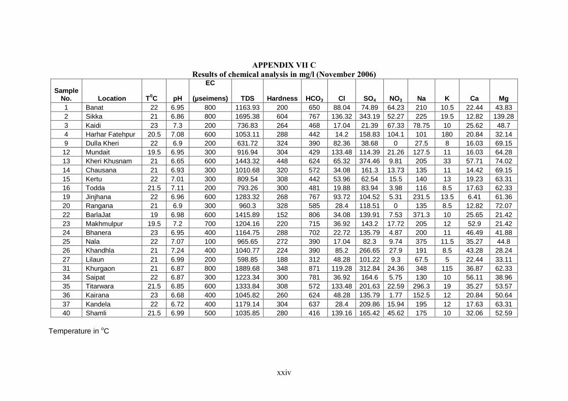
xxiv
APPENDIX VII C Results of chemical analysis in mg/l (November 2006)
Sample No. Location T
0C pH
EC
(µseimens) TDS Hardness HCO3 Cl SO4 NO3 Na K Ca Mg
1 Banat 22 6.95 800 1163.93 200 650 88.04 74.89 64.23 210 10.5 22.44 43.83
2 Sikka 21 6.86 800 1695.38 604 767 136.32 343.19 52.27 225 19.5 12.82 139.28
3 Kaidi 23 7.3 200 736.83 264 468 17.04 21.39 67.33 78.75 10 25.62 48.7
4 Harhar Fatehpur 20.5 7.08 600 1053.11 288 442 14.2 158.83 104.1 101 180 20.84 32.14
9 Dulla Kheri 22 6.9 200 631.72 324 390 82.36 38.68 0 27.5 8 16.03 69.15
12 Mundait 19.5 6.95 300 916.94 304 429 133.48 114.39 21.26 127.5 11 16.03 64.28
13 Kheri Khusnam 21 6.65 600 1443.32 448 624 65.32 374.46 9.81 205 33 57.71 74.02
14 Chausana 21 6.93 300 1010.68 320 572 34.08 161.3 13.73 135 11 14.42 69.15
15 Kertu 22 7.01 300 809.54 308 442 53.96 62.54 15.5 140 13 19.23 63.31
16 Todda 21.5 7.11 200 793.26 300 481 19.88 83.94 3.98 116 8.5 17.63 62.33
19 Jinjhana 22 6.96 600 1283.32 268 767 93.72 104.52 5.31 231.5 13.5 6.41 61.36
20 Rangana 21 6.9 300 960.3 328 585 28.4 118.51 0 135 8.5 12.82 72.07
22 BarlaJat 19 6.98 600 1415.89 152 806 34.08 139.91 7.53 371.3 10 25.65 21.42
23 Makhmulpur 19.5 7.2 700 1204.16 220 715 36.92 143.2 17.72 205 12 52.9 21.42
24 Bhanera 23 6.95 400 1164.75 288 702 22.72 135.79 4.87 200 11 46.49 41.88
25 Nala 22 7.07 100 965.65 272 390 17.04 82.3 9.74 375 11.5 35.27 44.8
26 Khandhla 21 7.24 400 1040.77 224 390 85.2 266.65 27.9 191 8.5 43.28 28.24
27 Lilaun 21 6.99 200 598.85 188 312 48.28 101.22 9.3 67.5 5 22.44 33.11
31 Khurgaon 21 6.87 800 1889.68 348 871 119.28 312.84 24.36 348 115 36.87 62.33
34 Saipat 22 6.87 300 1223.34 300 781 36.92 164.6 5.75 130 10 56.11 38.96
35 Titarwara 21.5 6.85 600 1333.84 308 572 133.48 201.63 22.59 296.3 19 35.27 53.57
36 Kairana 23 6.68 400 1045.82 260 624 48.28 135.79 1.77 152.5 12 20.84 50.64
37 Kandela 22 6.72 400 1179.14 304 637 28.4 209.86 15.94 195 12 17.63 63.31
40 Shamli 21.5 6.99 500 1035.85 280 416 139.16 165.42 45.62 175 10 32.06 52.59
Temperature in oC
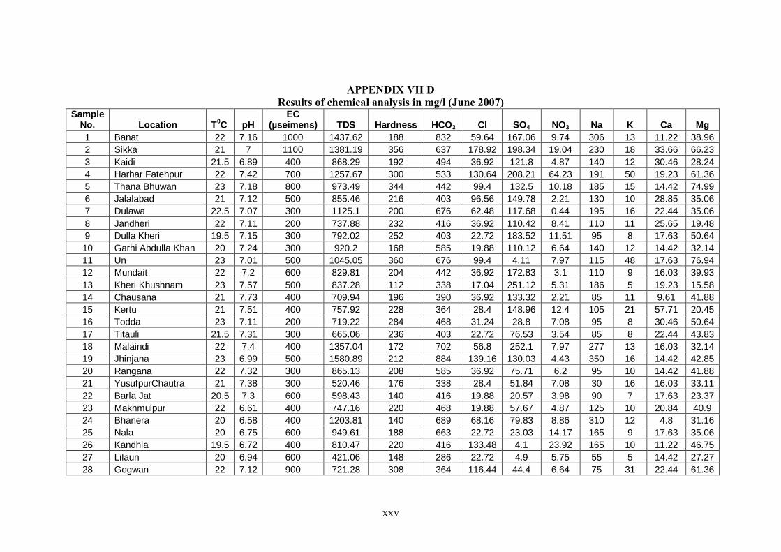
xxv
APPENDIX VII D Results of chemical analysis in mg/l (June 2007)
Sample No. Location T
0C pH
EC (µseimens) TDS Hardness HCO3 Cl SO4 NO3 Na K Ca Mg
1 Banat 22 7.16 1000 1437.62 188 832 59.64 167.06 9.74 306 13 11.22 38.96
2 Sikka 21 7 1100 1381.19 356 637 178.92 198.34 19.04 230 18 33.66 66.23
3 Kaidi 21.5 6.89 400 868.29 192 494 36.92 121.8 4.87 140 12 30.46 28.24
4 Harhar Fatehpur 22 7.42 700 1257.67 300 533 130.64 208.21 64.23 191 50 19.23 61.36
5 Thana Bhuwan 23 7.18 800 973.49 344 442 99.4 132.5 10.18 185 15 14.42 74.99
6 Jalalabad 21 7.12 500 855.46 216 403 96.56 149.78 2.21 130 10 28.85 35.06
7 Dulawa 22.5 7.07 300 1125.1 200 676 62.48 117.68 0.44 195 16 22.44 35.06
8 Jandheri 22 7.11 200 737.88 232 416 36.92 110.42 8.41 110 11 25.65 19.48
9 Dulla Kheri 19.5 7.15 300 792.02 252 403 22.72 183.52 11.51 95 8 17.63 50.64
10 Garhi Abdulla Khan 20 7.24 300 920.2 168 585 19.88 110.12 6.64 140 12 14.42 32.14
11 Un 23 7.01 500 1045.05 360 676 99.4 4.11 7.97 115 48 17.63 76.94
12 Mundait 22 7.2 600 829.81 204 442 36.92 172.83 3.1 110 9 16.03 39.93
13 Kheri Khushnam 23 7.57 500 837.28 112 338 17.04 251.12 5.31 186 5 19.23 15.58
14 Chausana 21 7.73 400 709.94 196 390 36.92 133.32 2.21 85 11 9.61 41.88
15 Kertu 21 7.51 400 757.92 228 364 28.4 148.96 12.4 105 21 57.71 20.45
16 Todda 23 7.11 200 719.22 284 468 31.24 28.8 7.08 95 8 30.46 50.64
17 Titauli 21.5 7.31 300 665.06 236 403 22.72 76.53 3.54 85 8 22.44 43.83
18 Malaindi 22 7.4 400 1357.04 172 702 56.8 252.1 7.97 277 13 16.03 32.14
19 Jhinjana 23 6.99 500 1580.89 212 884 139.16 130.03 4.43 350 16 14.42 42.85
20 Rangana 22 7.32 300 865.13 208 585 36.92 75.71 6.2 95 10 14.42 41.88
21 YusufpurChautra 21 7.38 300 520.46 176 338 28.4 51.84 7.08 30 16 16.03 33.11
22 Barla Jat 20.5 7.3 600 598.43 140 416 19.88 20.57 3.98 90 7 17.63 23.37
23 Makhmulpur 22 6.61 400 747.16 220 468 19.88 57.67 4.87 125 10 20.84 40.9
24 Bhanera 20 6.58 400 1203.81 140 689 68.16 79.83 8.86 310 12 4.8 31.16
25 Nala 20 6.75 600 949.61 188 663 22.72 23.03 14.17 165 9 17.63 35.06
26 Kandhla 19.5 6.72 400 810.47 220 416 133.48 4.1 23.92 165 10 11.22 46.75
27 Lilaun 20 6.94 600 421.06 148 286 22.72 4.9 5.75 55 5 14.42 27.27
28 Gogwan 22 7.12 900 721.28 308 364 116.44 44.4 6.64 75 31 22.44 61.36
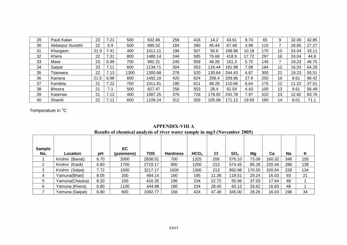
xxvi
29 Pauti Kalan 23 7.21 500 632.46 256 416 14.2 43.61 9.74 65 9 32.06 42.85
30 Akbarpur Sunethi 22 6.9 500 685.02 184 390 45.44 67.48 3.98 115 7 28.85 27.27
31 Khurgaon 21.5 7.41 400 1011.11 196 507 56.8 199.98 10.18 170 10 24.04 33.11
32 Khera 22 7.31 800 1480.14 244 585 76.68 418.9 17.72 297 16 24.04 44.8
33 Mawi 23 6.99 700 992.31 240 559 48.28 161.3 5.75 145 7 19.23 46.75
34 Saipat 23 7.11 600 1134.71 304 553 116.44 181.88 7.08 184 12 16.03 64.28
35 Titarwara 22 7.13 1300 1300.68 276 520 130.64 244.43 4.87 305 21 19.23 55.51
36 Kairana 21.5 6.98 600 1492.19 420 624 258.4 209.86 27.9 250 16 9.61 96.42
37 Kandela 21 7.22 700 1011.81 180 611 48.28 110.66 6.64 175 12 11.22 37.01
38 Bhoora 21 7.1 500 827.47 256 553 28.4 62.54 4.43 100 13 9.61 56.49
39 Kaserwa 21 7.12 400 1587.25 376 728 178.92 242.78 7.97 310 23 12.82 83.76
40 Shamli 22 7.11 600 1108.24 312 559 105.08 171.12 19.93 160 14 8.01 71.1
Temperature in oC
APPENDIX-VIII A Results of chemical analysis of river water sample in mg/l (November 2005)
Sample No. Location pH
EC (µsiemens) TDS Hardness HCO3 Cl SO4 Mg Ca Na K
1 Krishni (Banat) 6.70 2000 2838.51 700 1325 206 576.10 73.09 160.32 348 150
2 Krishni (Kaidi) 6.80 1700 2719.17 900 1200 213 574.45 85.28 220.44 288 138
3 Krishni (Salpa) 7.72 1500 3217.17 1500 1300 213 850.98 170.55 320.64 228 134
4 Yamuna(Bhari) 8.05 200 484.14 160 195 11.36 118.51 29.24 16.03 93 21
5 Yamuna(Chautra) 8.20 100 416.35 196 234 22.72 55.96 37.03 17.64 48 1
6 Yamuna (Khera) 6.80 1100 444.98 180 234 28.40 83.12 33.62 16.83 48 1
7 Yamuna (Saipat) 6.80 600 1092.77 156 424 47.48 345.00 28.26 16.03 198 34
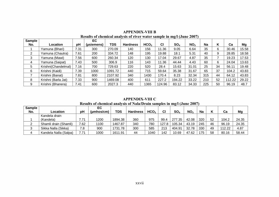
xxvii
APPENDIX-VIII B Results of chemical analysis of river water sample in mg/l (June 2007)
Sample No. Location pH
EC (µsiemens) TDS Hardness HCO3 Cl SO4 NO3 Na K Ca Mg
1 Yamuna (Bhari) 7.31 300 270.09 140 156 11.36 9.05 6.64 35 6 30.46 15.58
2 Yamuna (Chautra) 7.61 200 334.72 148 195 19.88 18.1 5.31 40 9 28.85 18.58
3 Yamuna (Mawi) 7.56 600 260.34 120 130 17.04 29.67 4.87 35 7 19.23 17.53
4 Yamuna (Saipat) 7.43 500 306.9 116 143 11.36 44.44 4.43 60 6 24.04 13.63
5 Krishni(Chandelmal) 7.16 700 729.63 220 520 28.4 15.63 31.01 25 34 56.11 19.48
6 Krishni (Kaidi) 7.39 1000 1091.72 440 715 59.64 35.38 31.67 65 37 104.2 43.83
7 Krishni (Banat) 7.81 800 2107.92 340 1430 170.4 8.23 32.34 315 44 64.12 43.83
8 Krishni (Barla Jat) 7.33 900 1469.08 400 611 227.2 194.22 33.22 210 52 112.22 29.22
9 Krishni (Bhanera) 7.41 600 2027.3 440 1365 124.96 83.12 34.33 225 50 96.19 48.7
APPENDIX-VIII C Results of chemical analysis of Nala/Drain samples in mg/l (June 2007)
Sample No. Location pH
EC (µmhos/cm) TDS Hardness HCO3 Cl SO4 NO3 Na K Ca Mg
1 Kandela drain (Kandela) 7.71 1200 1894.38 360 975 99.4 277.35 42.08 320 52 104.2 24.35
2 Shamli drain (Shamli) 7.62 1100 1467.87 340 780 127.8 105.34 43.19 245 46 96.19 24.35
3 Sikka Nalla (Sikka) 7.8 900 1731.78 300 585 213 404.91 32.78 330 49 112.22 4.87
4 Kandela Nalla (Salpa) 7.71 1000 1611.91 44 1040 142 10.69 47.62 175 58 80.16 58.44
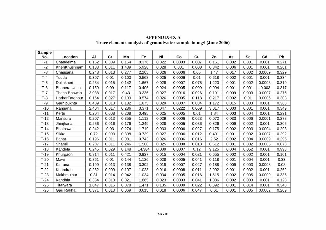
xxviii
APPENDIX-IX A Trace elements analysis of groundwater sample in mg/l (June 2006)
Sample
No. Location Al Cr Mn Fe Ni Co Cu Zn As Se Cd Pb
T-1 Chandelmal 0.162 0.009 0.164 0.376 0.022 0.0003 0.007 0.161 0.002 0.001 0.001 0.271
T-2 KheriKhushnam 0.183 0.011 1.439 5.928 0.028 0.001 0.008 0.842 0.006 0.001 0.001 0.261
T-3 Chausana 0.248 0.013 0.277 2.205 0.026 0.0006 0.05 1.47 0.017 0.002 0.0009 0.329
T-4 Todda 0.397 0.01 0.103 0.568 0.025 0.0006 0.01 0.618 0.002 0.001 0.001 0.334
T-5 Dullakheri 0.234 0.015 0.142 1.667 0.028 0.0007 0.075 1.223 0.001 0.002 0.0003 0.319
T-6 Bhanera Udha 0.159 0.09 0.117 0.406 0.024 0.0005 0.009 0.094 0.001 0.001 -0.003 0.317
T-7 Thana Bhawan 3.038 0.017 0.43 3.236 0.027 0.0016 0.026 0.191 0.009 0.003 0.0007 0.276
T-8 HarharFatehpur 0.164 0.027 0.109 0.574 0.026 0.0005 0.118 0.217 0.002 0.01 0.0006 0.303
T-9 Garhipukhta 0.409 0.013 0.132 1.875 0.029 0.0007 0.034 1.172 0.015 0.003 0.001 0.368
T-10 Rangana 2.404 0.017 0.286 3.371 0.047 0.0222 0.069 3.017 0.003 0.001 0.001 0.349
T-11 Kertu 0.204 0.008 0.208 0.495 0.025 0.0005 0.01 1.84 0.003 0.004 0.001 0.291
T-12 Mansura 0.207 0.013 0.355 1.112 0.029 0.0006 0.023 0.072 0.033 0.006 0.0001 0.278
T-13 Jhinjhana 0.256 0.016 0.176 1.249 0.028 0.0005 0.036 0.826 0.009 0.002 0.001 0.306
T-14 Bhainswal 0.242 0.03 0.274 1.719 0.033 0.0006 0.027 0.175 0.002 0.003 0.0004 0.293
T-15 Sikka 0.72 0.093 0.308 0.739 0.027 0.0006 0.012 0.401 0.001 0.002 0.0007 0.292
T-16 Banat 0.196 0.011 0.081 0.743 0.026 0.0006 0.016 2.52 0.002 0.004 0.0009 0.295
T-17 Shamli 0.207 0.011 0.246 1.568 0.025 0.0008 0.013 0.612 0.001 0.002 0.0005 0.073
T-18 Kandela 0.245 0.029 0.148 14.384 0.039 0.0007 0.12 9.125 0.004 0.052 0.001 0.998
T-19 Khurgaon 0.314 0.011 0.421 0.927 0.015 0.0004 0.021 0.655 0.002 0.002 0.001 0.101
T-20 Mawi 0.861 0.01 0.144 1.126 0.028 0.0005 0.041 0.118 0.001 0.004 0.001 0.33
T-21 Kairana 0.199 0.013 0.138 3.302 0.019 0.0007 0.027 0.188 0.009 0.003 0.0008 0.08
T-22 Khandrauli 0.232 0.009 0.107 1.023 0.016 0.0008 0.011 2.992 0.001 0.002 0.001 0.262
T-23 Makhmulpur 0.31 0.014 0.042 1.034 0.034 0.0005 0.016 1.615 0.002 0.005 0.0009 0.336
T-24 Kandhla 0.354 0.013 0.021 1.865 0.023 0.0003 0.041 1.036 0.002 0.003 0.001 0.128
T-25 Titarwara 1.047 0.015 0.078 1.471 0.135 0.0009 0.022 0.392 0.001 0.014 0.001 0.348
T-26 Gari Rakha 0.371 0.013 0.069 0.615 0.018 0.0006 0.047 0.61 0.001 0.005 0.0002 0.209
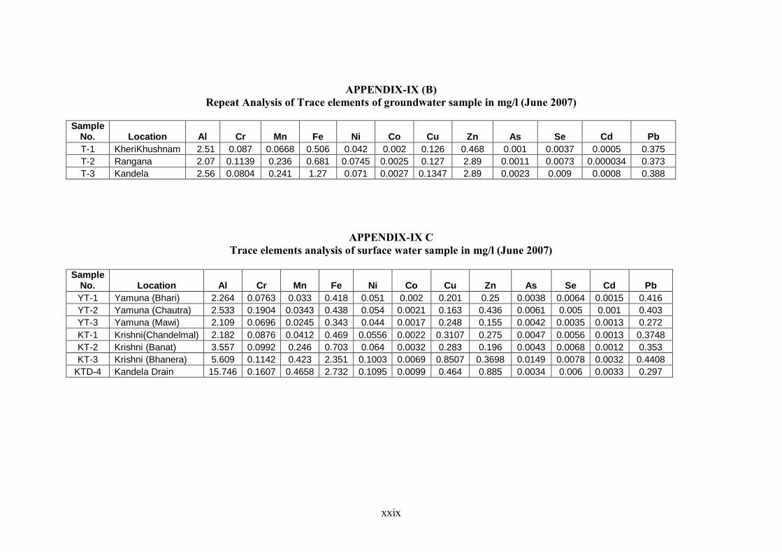
xxix
APPENDIX-IX (B) Repeat Analysis of Trace elements of groundwater sample in mg/l (June 2007)
Sample
No. Location Al Cr Mn Fe Ni Co Cu Zn As Se Cd Pb
T-1 KheriKhushnam 2.51 0.087 0.0668 0.506 0.042 0.002 0.126 0.468 0.001 0.0037 0.0005 0.375
T-2 Rangana 2.07 0.1139 0.236 0.681 0.0745 0.0025 0.127 2.89 0.0011 0.0073 0.000034 0.373
T-3 Kandela 2.56 0.0804 0.241 1.27 0.071 0.0027 0.1347 2.89 0.0023 0.009 0.0008 0.388
APPENDIX-IX C Trace elements analysis of surface water sample in mg/l (June 2007)
Sample
No. Location Al Cr Mn Fe Ni Co Cu Zn As Se Cd Pb
YT-1 Yamuna (Bhari) 2.264 0.0763 0.033 0.418 0.051 0.002 0.201 0.25 0.0038 0.0064 0.0015 0.416
YT-2 Yamuna (Chautra) 2.533 0.1904 0.0343 0.438 0.054 0.0021 0.163 0.436 0.0061 0.005 0.001 0.403
YT-3 Yamuna (Mawi) 2.109 0.0696 0.0245 0.343 0.044 0.0017 0.248 0.155 0.0042 0.0035 0.0013 0.272
KT-1 Krishni(Chandelmal) 2.182 0.0876 0.0412 0.469 0.0556 0.0022 0.3107 0.275 0.0047 0.0056 0.0013 0.3748
KT-2 Krishni (Banat) 3.557 0.0992 0.246 0.703 0.064 0.0032 0.283 0.196 0.0043 0.0068 0.0012 0.353
KT-3 Krishni (Bhanera) 5.609 0.1142 0.423 2.351 0.1003 0.0069 0.8507 0.3698 0.0149 0.0078 0.0032 0.4408
KTD-4 Kandela Drain 15.746 0.1607 0.4658 2.732 0.1095 0.0099 0.464 0.885 0.0034 0.006 0.0033 0.297
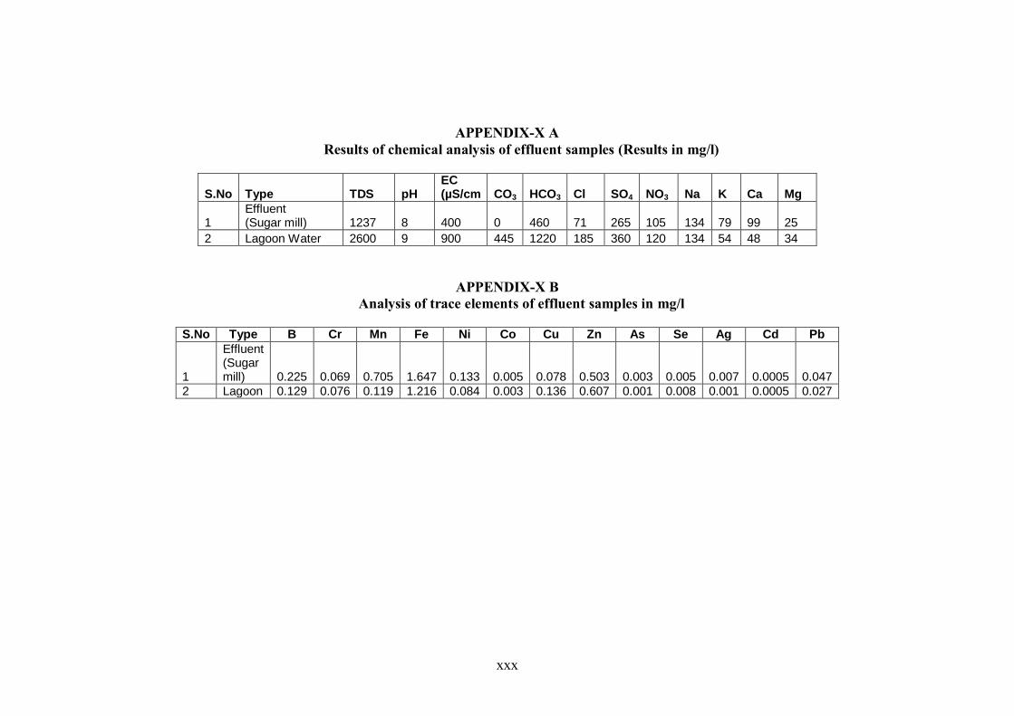
xxx
APPENDIX-X A
Results of chemical analysis of effluent samples (Results in mg/l)
S.No Type TDS pH EC (µS/cm CO3 HCO3 Cl SO4 NO3 Na K Ca Mg
1 Effluent (Sugar mill) 1237 8 400 0 460 71 265 105 134 79 99 25
2 Lagoon Water 2600 9 900 445 1220 185 360 120 134 54 48 34
APPENDIX-X B Analysis of trace elements of effluent samples in mg/l
S.No Type B Cr Mn Fe Ni Co Cu Zn As Se Ag Cd Pb
1
Effluent (Sugar mill) 0.225 0.069 0.705 1.647 0.133 0.005 0.078 0.503 0.003 0.005 0.007 0.0005 0.047
2 Lagoon 0.129 0.076 0.119 1.216 0.084 0.003 0.136 0.607 0.001 0.008 0.001 0.0005 0.027
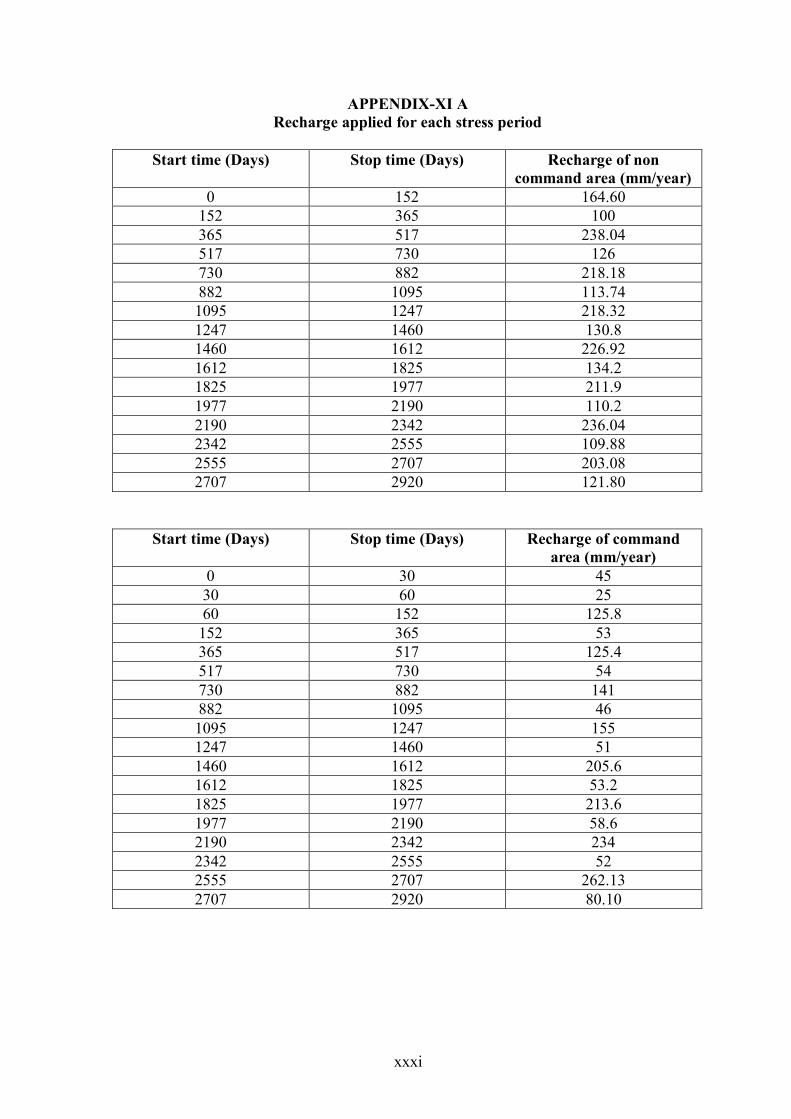
xxxi
APPENDIX-XI A Recharge applied for each stress period
Start time (Days) Stop time (Days) Recharge of non
command area (mm/year) 0 152 164.60
152 365 100 365 517 238.04 517 730 126 730 882 218.18 882 1095 113.74 1095 1247 218.32 1247 1460 130.8 1460 1612 226.92 1612 1825 134.2 1825 1977 211.9 1977 2190 110.2 2190 2342 236.04 2342 2555 109.88 2555 2707 203.08 2707 2920 121.80
Start time (Days) Stop time (Days) Recharge of command area (mm/year)
0 30 45 30 60 25 60 152 125.8
152 365 53 365 517 125.4 517 730 54 730 882 141 882 1095 46 1095 1247 155 1247 1460 51 1460 1612 205.6 1612 1825 53.2 1825 1977 213.6 1977 2190 58.6 2190 2342 234 2342 2555 52 2555 2707 262.13 2707 2920 80.10
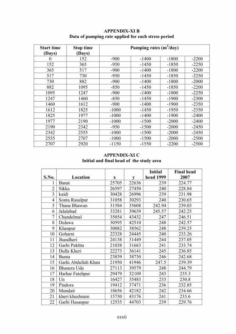
xxxii
APPENDIX-XI B Data of pumping rate applied for each stress period
Start time
(Days) Stop time
(Days) Pumping rates (m3/day)
0 152 -900 -1400 -1800 -2200 152 365 -950 -1450 -1850 -2250 365 517 -900 -1400 -1800 -2200 517 730 -950 -1450 -1850 -2250 730 882 -900 -1400 -1800 -2000 882 1095 -850 -1450 -1850 -2200
1095 1247 -900 -1400 -1800 -2250 1247 1460 -850 -1450 -1900 -2300 1460 1612 -900 -1400 -1900 -2350 1612 1825 -1000 -1450 -1950 -2350 1825 1977 -1000 -1400 -1900 -2400 1977 2190 -1000 -1500 -2000 -2400 2190 2342 -950 -1500 -2000 -2450 2342 2555 -1000 -1500 -2000 -2450 2555 2707 -1000 -1500 -2000 -2500 2707 2920 -1150 -1550 -2200 -2500
APPENDIX-XI C
Initial and final head of the study area
S.No. Location x y Initial
head 1999 Final head
2007 1 Banat 25705 22636 239 224.77 2 Sikka 26597 27450 240 228.84 3 kaidi 30428 26996 239 231.98 4 Sonta Rasulpur 31058 30293 240 230.65 5 Thana Bhawan 31584 35608 242.94 239.03 6 Jalalabad 33281 39639 245.57 242.25 7 Chandelmal 35054 43432 247 246.51 8 Dulawa 30595 42510 248 242.57 9 Khanpur 30082 38562 248 239.25
10 Goharni 22328 24445 240 233.26 11 Jhandheri 24138 31449 244 237.05 12 Garhi Pukhta 21038 31663 241 233.74 13 Dulla Kheri 22273 36141 245 236.85 14 Bunta 23839 38730 246 242.68 15 Garhi Abdullah Khan 21950 41946 247.5 239.39 16 Bhanera Uda 27113 39579 248 244.79 17 Harhar Fatehpur 29479 32109 243 235.3 18 Un 16427 35483 233 230.8 19 Pindora 19412 37471 236 232.85 20 Mundait 18656 42182 242 234.66 21 kheri khushnam 15730 43176 241 233.6 22 Garhi Hasanpur 12535 44703 239 229.76
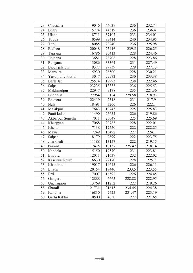
xxxiii
23 Chausana 9046 44039 236 232.74 24 Bhari 5774 44319 236 236.4 25 Ulahni 8711 37107 233 234.01 26 Todda 10599 39414 240 234.95 27 Titoli 18085 23240 236 225.98 28 Badheo 20048 25416 239.5 226.25 29 Taprana 16786 25413 228 224.46 30 Jinjhana 13681 28708 228 223.86 31 Rangana 13086 33364 231 227.49 32 Bipur jalalpur 9377 29739 229 227.13 33 Mansura 5930 28500 228 230.21 34 Yusufpur choutra 3047 29972 230 233.38 35 Barla Jat 25514 17993 238 222.46 36 Salpa 23235 13333 236 225.53 37 Makhmulpur 22947 9178 235 221.36 38 Bhabhisa 22964 6184 229.58 218.93 39 Bhanera 22419 2518 231 217.9 40 Nala 18491 3266 226 222.1 41 Malakpur 17643 10743 225 225.83 42 Pauti kalan 11490 25654 226 219.86 43 Akbarpur Sunethi 7011 25047 225 225.69 44 Khurgyan 7068 20783 228 222.01 45 Khera 7138 17550 222 222.25 46 Mawi 7249 13492 227 224.1 47 Saipat 8179 9899 222 223.75 48 Jharkhedi 11188 13157 222 219.15 49 kairana 12475 16137 225.42 218.14 50 Kandela 15150 19570 231 223.81 51 Bhoora 12011 21639 232 222.02 52 Kaserwa Khurd 16630 22170 228 225.7 53 Khandrauli 19017 14645 226 226.11 54 Lilaun 20154 18440 233.5 223.55 55 Erti 17007 16592 226 224.45 56 Gangeru 12888 6665 228.82 222.95 57 Unchagaon 13769 11252 222 219.26 58 Shamli 21731 21615 234.45 224.38 59 Kandhla 16830 7425 231.47 223.19 60 Garhi Rakha 10500 4650 222 221.65
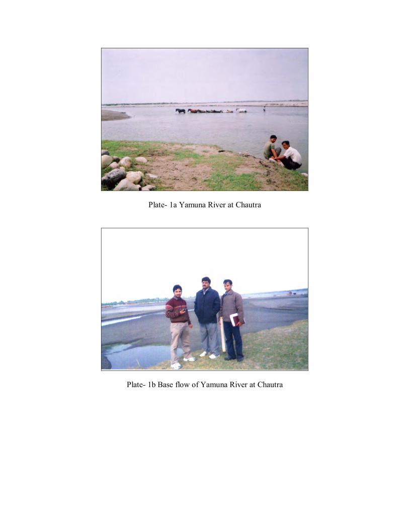
Plate- 1a Yamuna River at Chautra
Plate- 1b Base flow of Yamuna River at Chautra
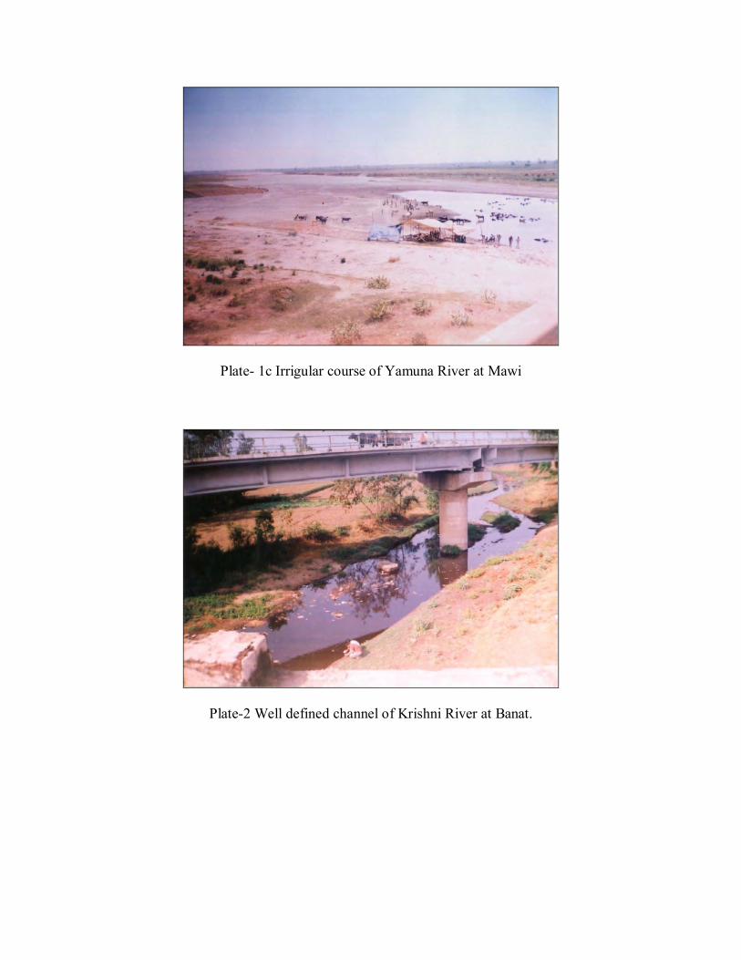
Plate- 1c Irrigular course of Yamuna River at Mawi
Plate-2 Well defined channel of Krishni River at Banat.
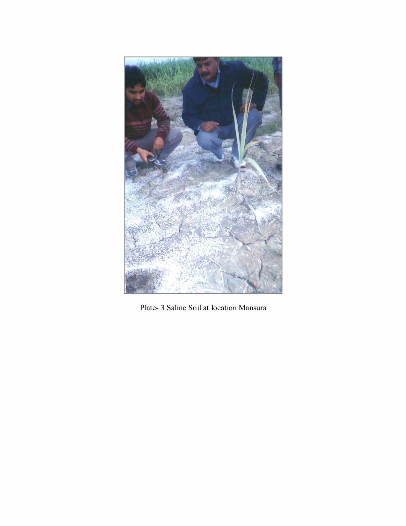
Plate- 3 Saline Soil at location Mansura
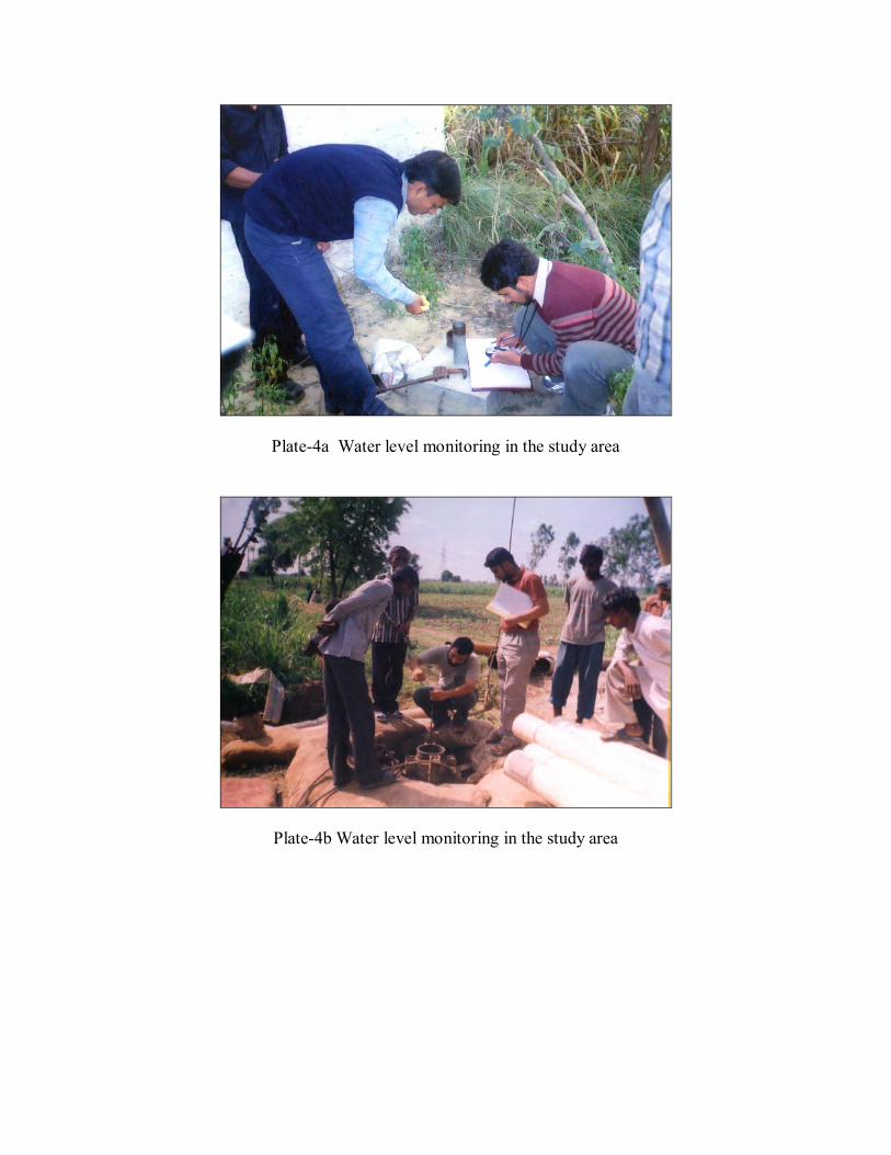
Plate-4a Water level monitoring in the study area
Plate-4b Water level monitoring in the study area
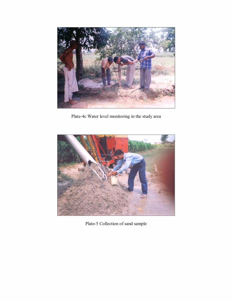
Plate-4c Water level monitoring in the study area
Plate-5 Collection of sand sample
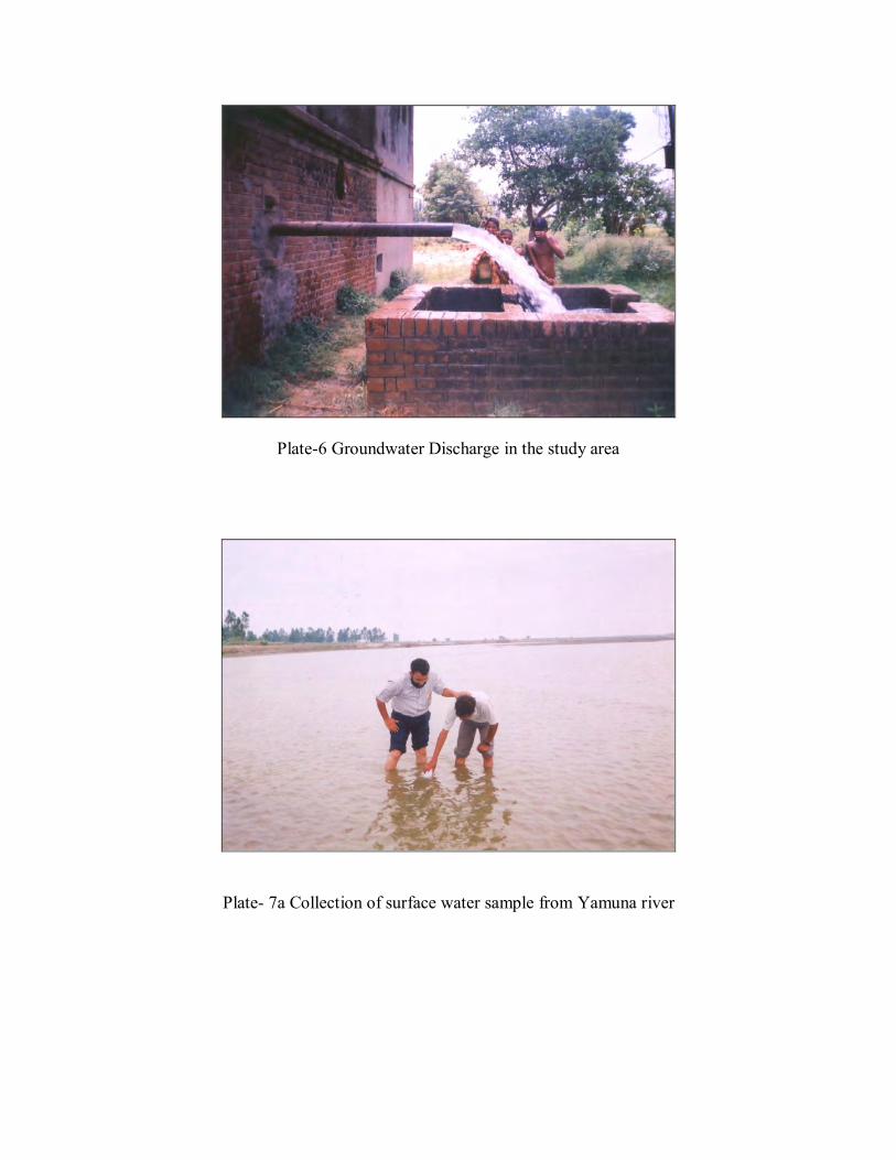
Plate-6 Groundwater Discharge in the study area
Plate- 7a Collection of surface water sample from Yamuna river
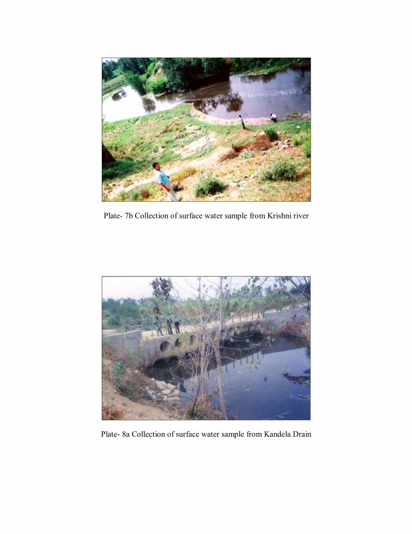
Plate- 7b Collection of surface water sample from Krishni river
Plate- 8a Collection of surface water sample from Kandela Drain
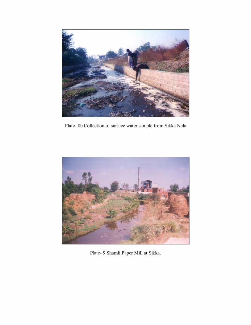
Plate- 8b Collection of surface water sample from Sikka Nala
Plate- 9 Shamli Paper Mill at Sikka.