Groundwater flow and reactive transport modelling in … · Den kemiska sammansättningen av...

Svensk Kärnbränslehantering ABSwedish Nuclear Fueland Waste Management Co

Box 250, SE-101 24 Stockholm Phone +46 8 459 84 00

R-14-19

Groundwater flow and reactive transport modelling in ConnectFlow

Steven Joyce, David Applegate, Peter Appleyard, Andrew Gordon, Tim Heath, Fiona Hunter, Jaap Hoek, Peter Jackson, David Swan, Hannah Woollard Amec Foster Wheeler

January 2015

R-14-19

Tänd ett lager: P, R eller TR.

Groundwater flow and reactive transport modelling in ConnectFlow

Steven Joyce, David Applegate, Peter Appleyard, Andrew Gordon, Tim Heath, Fiona Hunter, Jaap Hoek, Peter Jackson, David Swan, Hannah Woollard Amec Foster Wheeler

ISSN 1402-3091SKB R-14-19ID 1436659

January 2015

This report concerns a study which was conducted for Svensk Kärnbränslehantering AB (SKB). The conclusions and viewpoints presented in the report are those of the authors. SKB may draw modified conclusions, based on additional literature sources and/or expert opinions.

A pdf version of this document can be downloaded from www.skb.se.

© 2015 Svensk Kärnbränslehantering AB

SKB R-14-19 3

Abstract

Hydrogeochemistry is recognised as an important consideration for the safety of subterranean radioactive waste repositories. The chemical composition of the groundwater can have an impact on the performance of the engineered barrier system. The groundwater composition around a repository is dependent on groundwater flow and transport and chemical reactions. In the site descriptive mod-elling and SR-Site safety assessment for Forsmark, however, due to the computational demands of coupling these processes, the calculation of chemical reactions has been treated separately from the calculation of groundwater flow and transport. At best, these processes have been loosely coupled by importing the flow fields or compositions from flow and transport calculations into geochemical calculations at a selection of discrete locations and times, or have been based on simple 1D, 2D or small-scale reactive transport models. However, groundwater flow, transport and geochemistry are continuous coupled processes and so the loosely coupled methodology may fail to capture the processes adequately. This has been recognised by reviewers and identified as a priority for both SKB’s and Posiva’s future research programmes.

ConnectFlow is groundwater flow and transport software that has a comprehensive range of facilities to represent a number of hydrogeological situations and concepts at a range of scales. Its capabilities and flexibility have led to its extensive use to provide input to SKB’s and Posiva’s site descriptive modelling and safety assessment programmes for the Forsmark and Olkiluoto spent nuclear fuel repositories respectively. This report describes the implementation of chemical reaction calculations coupled with multi-component solute transport within ConnectFlow. The implementation allows the flexible specification of the spatial distribution of chemical species, minerals and ion exchangers for use in chemical equilibration reactions. The groundwater flow calculations and transport of chemical species are carried out by ConnectFlow and the chemical reactions for each time step are performed by the iPhreeqc software library, which provides an interface to the widely used PHREEQC geo-chemical software. The two software products are closely integrated so that simulations can be run over many time steps without any user intervention. Output options allow the quantities of selected chemical species at specified locations and times to be output for analysis and visualisation.

Also implemented is a new method for carrying out the calculation of the diffusion of solutes into the rock matrix based on a finite volume scheme. The new method allows both chemistry and diffusion to be carried out in the rock matrix, whereas the original method for modelling rock matrix diffusion in ConnectFlow is only appropriate for non-reacting species. Additionally, the new method allows extra flexibility in defining the discretisation of the rock matrix.

The computational performance of the reactive transport implementation is critical in determining its applicability to large scale problems. A combination of efficient implementation and parallelisation of the key rate determining processes gives an implementation that produces good performance even for large regional models.

The implementation is verified for a range of chemical reactions by comparison with the Phast and TOUGHREACT software products. Excellent agreement in results was found for the range of cases considered.

Illustrative examples of palaeo-climate calculations of the Forsmark and Olkiluoto sites are carried out to assess the applicability of the implementation to these types of models.

The implementation and application examples presented here demonstrate tangible progress against SKB’s and Posiva’s stated research priorities. In particular, a capability is provided to model reactive transport in a wide variety of situations by coupling ConnectFlow’s powerful groundwater flow and transport capabilities with the widely used and flexible geochemical reaction capabilities of PHREEQC.

4 SKB R-14-19

Sammanfattning

Hydrogeokemi utgör en viktig faktor för säkerheten av underjordiska förvar för radioaktivt avfall. Den kemiska sammansättningen av grundvattnet kan ha en inverkan på funktionen av det tekniska barriärsystemet. Grundvattensammansättningen runt ett slutförvar är beroende av grundvatten flöde och transport samt kemiska reaktioner. Inom den platsbeskrivande modelleringen och säkerhets-analysen SR-Site för Forsmark, på grund av de tunga beräkningarna kopplade till kemiska reaktioner, har dessa behandlats separat från simulering av grundvattenflöde och transport. I bästa fall har dessa processer varit löst kopplade genom att importera flödesfält eller sammansättningar från flödes- och transportberäkningar i geokemiska beräkningar på ett urval av diskreta platser och tider, eller har de baserats på enkla 1D, 2D eller småskaliga reaktiva transportmodeller. Men grundvattenflöde, transport och geokemi är kontinuerliga kopplade processer och därför kan den löst kopplade metoden misslyckas med att fånga processer på ett tillfredsställande sätt. Detta har uppmärk sammats av granskare och identifierades som en prioriterad fråga för både SKB: s och Posivas framtida forsknings program.

ConnectFlow är en programvara för grundvattenflöde och transport samt har ett omfattande utbud av faciliteter för att representera ett antal hydrogeologiska situationer och begrepp på en rad olika skalor. Dess kapacitet och flexibilitet har lett till dess omfattande användning för att ge underlag till SKB: s och Posivas program för platsbeskrivande modellering och säkerhetsbedömning av förvar för använt kärnbränsle i Forsmark respektive Olkiluoto. Denna rapport beskriver implementeringen av kemiska reaktionsberäkningar i kombination med flerkomponentstransport av lösta ämnen inom ConnectFlow. Implementeringen möjliggör flexibel specifikation av den rumsliga fördelningen av kemiska ämnen, mineraler och jonbytare för användningen av kemiska jämviktsreaktioner. Grundvattenflödesberäkningar och transport av kemiska ämnen utförs av ConnectFlow och de kemiska reaktionerna för varje tidssteg utförs av programvarubiblioteket iPhreeqc, vilket ger ett gränssnitt till den flitigt använda programvaran för geokemiska beräkningar PHREEQC. De två mjukvaruprodukterna är nära integrerade så att simuleringar kan köras under många tidssteg utan några åtgärder från användaren. Utskriftsalternativen tillåter att mängder av utvalda kemiska ämnen, på angivna platser och tider, matas ut för analys och visualisering.

Dessutom är en ny metod implementerad för att utföra beräkningen av diffusion av lösta ämnen in i bergmatrisen baserat på en finit volymsmetod. Den nya metoden möjliggör både kemiska reaktioner och diffusion i bergmatrisen, emedan den ursprungliga metoden för modellering av matrisdiffusion i ConnectFlow är endast lämplig för icke-reagerande ämnen. Den nya metoden ger dessutom extra flexibilitet för att definiera diskretiseringen av bergmatrisen.

Datorprestanda är avgörande vid genomförande av reaktiva transportberäkningar och för att bestämma dess tillämpbarhet på storskaliga problem. En kombination av en effektiv implementering och parallellisering av de viktigaste hastighetsbestämmande processerna ger en programvara som ger bra prestanda även för stora regionala modeller.

Implementeringen verifieras för ett spann av kemiska reaktioner och har jämförts med programmen Phast och TOUGHREACT. En utmärkt överenstämmelse konstaterades i de olika fallen.

Belysande exempel inom paleo-klimatberäkningar för platserna Forsmark och Olkiluoto har genom-förts för att bedöma lämpligheten av implementeringen för denna typ av beräkningsmodeller.

De exempel på implementering och tillämpning som presenteras här visar påtagliga framsteg inom SKB: s och Posivas uttalade forskningsprioriteringar. I synnerhet, tillhandahålls nu en möjlighet att modellera reaktiv transport, i en mängd olika situationer, genom att koppla ConnectFlows kraftfulla grundvattenflödes- och transportfunktioner med den vitt använda och flexibla geokemiska reaktions-kapaciteten i PHREEQC.

SKB R-14-19 5

Contents

1 Introduction 71.1 Background 71.2 Scope 81.3 Approach 91.4 Verification 11

2 Concepts 132.1 Groundwater flow 132.2 Solute transport 132.3 Rock matrix diffusion 142.4 Chemical reactions 15

2.4.1 Component transport 152.4.2 Reference waters 162.4.3 Initial conditions and boundary conditions 162.4.4 Initial chemical equilibration 162.4.5 Chemical equilibration 172.4.6 Charge balancing 172.4.7 Negative concentrations 172.4.8 Calculation thresholds 182.4.9 Calculation of non-master species 18

3 Mineral equilibration reactions 193.1 Context 193.2 Implementation 19

3.2.1 Mineral quantities 203.2.2 Pore-clogging 20

3.3 Verification 213.3.1 Calcite equilibration 223.3.2 Calcite precipitation 243.3.3 Calcite pore clogging 253.3.4 Calcite and pyrite equilibration 283.3.5 Olkiluoto equilibration 303.3.6 Forsmark equilibration 30

4 Ion exchange reactions 334.1 Context 334.2 Implementation 334.3 Verification 33

4.3.1 Ion exchange only 344.3.2 Ion exchange with mineral equilibration 37

5 Rock matrix diffusion 415.1 Introduction 415.2 Finite volume rock matrix diffusion 415.3 Implementation of finite volume RMD in ConnectFlow 42

5.3.1 Finite volume discretisation 425.3.2 Chemistry with rock matrix diffusion 44

5.4 Verification 445.4.1 Reference water non-reactive transport 445.4.2 Multi-component solute transport and equilibration with calcite 47

6 Performance and parallelisation 516.1 Chemistry and equation assembly 516.2 Rock matrix diffusion 54

7 Applications 577.1 Forsmark palaeo-climate calculations 57

6 SKB R-14-19

7.1.1 Background 577.1.2 Hydrogeological Conceptual Model 577.1.3 Hydrogeochemical Conceptual Model 607.1.4 Numerical Model 617.1.5 Effective porosity model 637.1.6 Rock matrix diffusion model 69

7.2 Olkiluoto palaeo-climate calculations 727.2.1 Background 727.2.2 Hydrogeological Conceptual Model 727.2.3 Hydrogeochemical Conceptual Model 737.2.4 Numerical Model 737.2.5 Results 75

8 Conclusions 81

References 83

Appendix A Component dependent density 87

SKB R-14-19 7

1 Introduction

1.1 BackgroundSKB and Posiva are considering deep geological repositories for spent nuclear fuel. The sites selected (Forsmark for SKB and Olkiluoto for Posiva) are both situated in crystalline rock, where groundwater flow is predominantly in fractures, but where the bulk of the porosity is in the rock matrix. The chemical composition of groundwater plays an important role in determining repository safety (SKB 2011, Posiva 2012a). In particular, the geochemical evolution of groundwater is one of the factors affecting the chemical stability of the engineered barrier systems, the resilience of the canisters and chemical buffering capacity of the host rock. The geochemical characteristics that are relevant to the safety assessment include salinity, redox potential, pH and the composition of a number of key chemical constituents (SKB 2011, Posiva 2012a). Additionally, construction activities, such as grouting, can modify the geochemical environment and thus have an impact on repository safety.

For the site descriptive modelling (SDM), SDM-Site Forsmark (Follin 2008), SDM-Site Laxemar (Rhén et al. 2009) and the Olkiluoto SDM (Posiva 2011, Hartley et al. 2012), palaeo-climate simula-tions were carried out as part of the confirmatory testing. The confirmatory testing was to establish whether the hydrogeological conceptual model and its numerical implementation at each site repro-duced present-day chemical compositions. These simulations were carried out for regional-scale equivalent continuous porous medium (ECPM) models, whose properties are based on an underlying discrete fracture network (DFN) as interpreted in site descriptive modelling. The models simulate the density-dependent transient evolution of the groundwater. The simulations represented the transport of chemical components in terms of the mixing of reference waters of specified compositions. The transport considered advection and dispersion in the fractured rock and included the effects of rock matrix diffusion (RMD), but did not consider the effects of chemical reactions. In reality, some com-ponents would react with one another and with minerals in the rock through which the groundwater flows. Neglecting the reactions means that there is some uncertainty about inferences based on the compositions of the reacting components, thus reducing confidence in whether processes affecting groundwater composition have been adequately represented.

Two-dimensional reactive transport modelling was carried out for the Simpevarp-Laxemar SDM by exporting a flow field from a density-dependent, steady-state groundwater flow model to a reactive transport model and then calculating the groundwater composition (Molinero et al. 2008). However, this modelling did not feed groundwater density changes back into the flow model and so only represented one-way coupling. It also did not consider the transient evolution of the system.

During the Forsmark safety assessment (SR-Site), a methodology was used for modelling the evolu-tion of hydrogeochemistry. The ConnectFlow regional-scale modelling calculated the evolution of groundwater flow and composition during the temperate climate period from 8000 BC to 12,000 AD (Joyce et al. 2010). In these calculations, the groundwater composition was described in terms of the combination of a number of reference waters, which were taken to be non-reactive. The outputs of this modelling were reference water fraction values for defined locations in the model for specified times. Chemistry calculations using the PHREEQC software (Parkhurst and Appelo 1999) were then carried out to determine the equilibrium chemical composition of the groundwater at selected locations (Salas et al. 2010). Note that only the chemical composition in the fractures was evaluated in PHREEQC and no attempt was made to carry out the calculations in the rock matrix, although reference water fractions were calculated by ConnectFlow for the rock matrix. It should be noted that most of the groundwater and most of the mineral volume and surface area with which the solutes can react is in the rock matrix, although many of the relevant reactions would only take place within the fractures or very close to the fractures within the rock matrix.

The methodology given above for SR-Site describes a decoupled process, where the reactive calculation of chemical composition for specified times is carried out separately from the transport calculations. In particular, this neglects changes to the environment experienced by the water as it moves, which could significantly affect the water composition. The altered composition would also affect groundwater density and hence solute transport, i.e. there is a two-way coupling. For example,

8 SKB R-14-19

if a certain mineral is precipitating along a flow path then a chemical reaction calculation carried out at the end of the path will give an incorrect result if the precipitation and change in solute composi-tion along the path have not been accounted for. Further, the minerals in the rocks at this location might differ from those along the path to the location. The groundwater composition calculated solely on the basis of the minerals at this location might therefore differ from that calculated taking into account the conditions experienced on the way to the location.

The use of cementitious material in repository construction and engineered structures can lead to the production of high pH leachates. In the long term, this can give rise to a plume of alkaline water that is transported by the groundwater flow system (e.g. Ewart et al. 1985, Grandia et al. 2010, Sidborn et al. 2014). The chemical interaction of this alkaline water with the engineered barrier systems and the host rock can impact repository performance. It is therefore important to gain a better understanding of the coupled transport and chemical processes that determine the composition and the pH of the water in contact with the repository system.

An approach where the transport and chemical processes are coupled would allow the composition of the chemical constituents to be modified by reactions while they are being transported, which gives more confidence that the relevant physical and chemical processes are being accounted for in deter-mining the distribution of chemical constituents. This ambition to develop new approaches to couple groundwater flow, solute transport and chemical reactions is stated in Section 25.3.3 of the SKB RD&D Programme (SKB 2010b). SSM’s review of the RD&D programme (SSM 2011) suggests such a capability is needed for safety assessment scenarios and for interpreting experiments at Äspö HRL, and urges SKB to make specific plans to achieve such an ambition. Similar issues are also likely to apply to the studies carried out by Posiva for the spent nuclear fuel repository at Olkiluoto (Posiva 2010). It is proposed that to achieve a coupled approach, chemical reaction calculations would be integrated with the ConnectFlow flow and transport calculations. The implementation of this would enable a number of modelling applications to be carried out for both Forsmark and Olkiluoto, including:

• Impact on regional-scale palaeo-climate calculations and future hydrogeochemical evolution of the sites.

• Effects of alkaline plumes generated from cementitious materials used in repository construction.

• Effect on the buffering capacity of minerals, e.g. calcite, if they are depleted due to dissolution and the implication for intrusion of dilute or acidic water, .e.g. under global warming conditions.

• Calculation of pH and redox conditions around the repository.

• The effects of dilute (and possibly oxygenated) water intrusion.

• The effects of groundwater intrusion under glacial conditions.

1.2 ScopeThe work reported here involves developing the capability to calculate chemical reactions in con-junction with groundwater flow and multi-component solute transport calculations in a continuous porous medium (CPM) model using the ConnectFlow software (AMEC 2012). This capability is demonstrated by applying it to regional-scale models of the transient evolution of groundwater composition. Typically, the models of interest for fractured crystalline rock use an equivalent continuous porous medium (ECPM) approach, where the properties of individual finite elements are based on the upscaling (Jackson et al. 2000) of an underlying discrete fracture network (DFN). The approach is applicable to scales from the detailed repository-scale up to the regional-scale and so computational efficiency is a key factor in determining success due to the large number of finite elements involved.

The following CPM features are now implemented in ConnectFlow (as integrated with iPhreeqc):

• Mineral equilibration reactions.

• Ion exchange reactions.

SKB R-14-19 9

• Spatially varying minerals.

• Formation of secondary minerals (minerals not initially present, but generated by chemical reac-tions) and their equilibration with solutes.

• Pore clogging (see below for discussion).

• Output of chemical composition, including non-master species (but not for the rock matrix).

• Rock matrix diffusion with chemistry.

Equilibration with mineral phases and ion exchange reactions have been chosen for implementation as two of the most relevant reaction types for larger-scale hydrogeology. The kinetics of chemical reactions have not been considered at this stage. The actual reactions available will be those present in the thermodynamic database supplied by the user. If the model has temperature variation then this will be reflected in the reaction temperatures if supported by the thermodynamic database. Typically the reactions will be valid up to ionic strengths of around 3 moles per litre for thermodynamic data-bases with appropriate ionic strength treatments and parameters (such as SIT), but only to 0.3 moles per litre when the Davies equation (as detailed in Equation (3-4) of Section 3) is used.

Treatment of spatially varying minerals and secondary minerals allows minerals to be created and depleted across the model and their quantities to be initially specified in a flexible way and the evolution of the quantities to be monitored. The pore-clogging facility allows the permeability and porosity of the rock to be modified due the volume changes in minerals as a result of precipitation or dissolution. Changes in porosity in the rock matrix are not currently included, although they might affect the diffusivity.

The output of non-master species provides access to the quantities of different chemical forms adopted by a master species, e.g. bicarbonate and carbonate in the case of carbon, and provides a flexible way of carrying out additional chemistry on solute compositions at selected times.

A new method of rock matrix diffusion within Connectflow, based on a finite volume method, has been developed that allows a flexible discretisation of the rock matrix and is compatible with chemi-cal reactions. The method allows chemical reactions to be carried out in the rock matrix, and the full solute composition, including its distance dependence, can be output for analysis. Pore clogging and the output of non-master species has not currently been implemented in the rock matrix.

1.3 ApproachConnectFlow has the ability to transport solutes in a number of ways, including transport of total salinity, transport of reference waters and transport of chemical components. For the site descriptive modelling and safety assessment modelling of Forsmark and Olkiluoto carried out using ConnectFlow, the evolution of groundwater in regional-scale palaeo-climate simulations was expressed in terms of the transport of reference waters (Follin 2008, Joyce et al. 2010, Hartley et al. 2012, 2013). Each reference water represents water of a particular origin, e.g. meteoric or glacial, and the composition of the groundwater at any point was expressed in terms of the mixing of fractions of the reference waters. However, the reference water approach is not appropriate when considering chemical reactions, as the concentration of any individual component at any point may change as a result of the reactions, so the composition of the reference water cannot then be maintained. Therefore the approach taken when carrying out chemical reactions has been to use the multi-component solute transport facility within ConnectFlow. Using this method, each component is transported separately and its mass fraction can be individually updated as a result of chemical reactions.

Solving the equations for groundwater flow and the transport of many chemical components in a fully coupled way would be computationally challenging. Therefore a sequential iteration method is used to implement operator splitting and decouple the transport calculations for the individual components from the flow calculations, giving improved efficiency at the expense of some accuracy. Multiple iterations over the sets of equations can be used to improve accuracy, with a corresponding cost in run time, although typically a single iteration is used for a system that is evolving slowly relative to the time step size.

10 SKB R-14-19

Rather than implement a completely new system for solving chemical reaction equations in ConnectFlow, an interface to PHREEQC is used. PHREEQC is an extensively used geochemi-cal software product that is capable of simulating a wide range of chemical reactions, including equilibration of aqueous solutions with minerals, ion exchanger materials, surface complexes, solid solutions and gases. It can also simulate kinetic non-equilibrium reactions. PHREEQC is freely available in the form of a C++ library called iPhreeqc (Charlton and Parkhurst 2011), with interfaces to other programming languages, such as Fortran. The interface to the library is in the form of a series of subroutines that allow text-based commands to be passed to PHREEQC using the PHREEQC command language. This allows the full capability of the PHREEQC software to be available via the library. Additional functions allow the state of the system to be updated and selected quantities to be output.

A set of Fortran modules have been created to provide an interface between ConnectFlow and the iPhreeqc library. These allow the chemical reactions to be specified in terms of the ConnectFlow command language (or via the graphical user interface). At this stage, the chemical reactions included are equilibration with mineral phases and ion exchange materials. Any PHREEQC-compatible thermodynamic database file can be specified for the chemical reaction calculations. The reactions are carried out at the end of each time step for a series of aqueous solutions, the composition of each being derived from the mass fractions of components present at each node where the components are defined in a CPM model. The results of the chemical reactions are then used to update the mass frac-tions of the components used in the flow and transport calculations for the next time step. The steps taken in a multi-component reactive transport calculation are shown in Figure 1-1.

Figure 1‑1. Flow diagram of reactive transport within ConnectFlow.

Loop over time steps

Iterate to required accuracy

Update density and viscosity

Initial set up of chemistry

Calculate groundwater flow

Calculate component transport

Calculate chemical reactions

Update component mass fractions

SKB R-14-19 11

1.4 VerificationThe coupled system of flow, transport and chemical reactions is difficult to verify by comparison with analytical methods due to the complexity of the system. Therefore, in order to verify the correct functioning of the reactive transport facility in ConnectFlow, comparisons are made for equivalent calculations using other software products that have already been verified.

One such product is Phast (Parkhurst et al. 2010). Phast also makes use of PHREEQC to carry out chemical reaction calculations and so is a good check that the integration between ConnectFlow and PHREEQC has been carried out correctly, provided that the transport calculations are equivalent. If the non-reactive transport is equivalent for a particular case and both software products use PHREEQC for the chemistry then identical results should be obtained. However, Phast is only able to model a fairly simple set of physical situations and so the verification is limited to the sub-set of systems that both software products can model. For example, Phast only supports models with constant fluid density.

Another reactive transport software product used for verification is TOUGHREACT (Xu et al. 2008). TOUGHREACT is based on the TOUGH2 multi-phase flow and transport software (Pruess et al. 1999). This uses different methods to calculate flow, transport and chemistry compared to ConnectFlow, so it is more difficult to obtain exactly equivalent models in the two software products. However, TOUGHREACT is useful to verify those features not available in Phast, such as pore clog-ging, and to provide an additional source of verification.

The verification cases are chosen to exercise the different functionality available in the ConnectFlow reactive transport implementation. The verification models are simple 3D columns of cells with one-dimensional uniform-density flow. This allows the verification to focus on the chemical reactions and the correct integration with ConnectFlow without the distraction of a complex flow system. The chemical reactions selected are those that are relevant to the Forsmark or Olkiluoto hydrogeochemi-cal settings. Likewise, the model properties are similar to those used in Forsmark or Olkiluoto models. Therefore, although only sub-sets of possible situations are verified, they are situations that are likely to be of relevance to SKB and Posiva.

SKB R-14-19 13

2 Concepts

2.1 Groundwater flowGroundwater flow in ConnectFlow (AMEC 2012) is expressed in terms of Darcy’s law

)( gq ρµ

-∇⋅-= Pk

(2-1)

and the equation for conservation of mass

0)()(

=⋅∇+∂

∂qρ

ρφtf (2-2)

where

• q is the specific discharge (or Darcy flux) [m/s],

• k is the equivalent permeability tensor due to the fractures carrying the flow [m2],

• μ is the groundwater viscosity [kg/m/s],

• P is the (total) pressure in the groundwater [N/m2],

• ρ is the groundwater density [kg/m3],

• g is the gravitational acceleration [m/s2],

• t is the time [s],

• ϕf is the kinematic porosity due to the fractures carrying the flow [-].

In general, the density and viscosity of the groundwater depend on temperature, pressure and total salinity. Temperature and salinity are in turn transported by the groundwater. When the variations in temperature or solute concentration are large enough to produce significant changes in density or viscosity, it is necessary to couple the solution of the groundwater flow problem to that of the heat or solute transport problem.

2.2 Solute transportConnectFlow calculates solute transport using the advection-dispersion equation

)()()(

cDct

cf

f ∇⋅⋅∇=⋅∇+∂

∂ρφρ

ρφq

(2-3)

where

• c is the solute mass fraction in the groundwater flowing through the fractures [-],

• D is the (effective) dispersion tensor [m2/s].

For a single transported component, Equations (2-1), (2-2) and (2-3) can be solved in ConnectFlow as a coupled set of equations. However, for the transport of many components it is not usually numerically or computationally practical to solve the full set of coupled equations. In this case, sequential iteration can be used as an operator splitting method to decouple the equations and solve each groundwater flow and transport equation separately (Saaltink et al. 2001). Using this method, each variable is solved for independently while holding the other variables constant, which effectively linearises the system for increased computational efficiency. Multiple iterations of the sequence of equations can be carried out for increased accuracy at the expense of computational time, but normally a single iteration is sufficient for a system that is evolving slowly relative to the time step size.

14 SKB R-14-19

2.3 Rock matrix diffusionRock matrix diffusion (RMD) (Neretnieks 1980) is the process of diffusion from fracture water into the less mobile water within the rock matrix. The pore space within the rock matrix provides the majority of the volume and reactive surface area available to groundwater and so is an important site for chemical reactions to occur. RMD thus effectively provides a retardation mechanism for the transport of solutes.

The equations for groundwater flow and solute transport in the fracture system for a ConnectFlow CPM model on a large scale, with solute diffusion into the rock matrix between parallel equally spaced fractures (Hoch and Jackson 2004, based on Carrera et al. 1998), are:

0

)()()(

=∂′∂+∇⋅⋅∇=⋅∇+

∂∂

wif

f

wcDcDc

tc

σρρφρρφ

q

(2-4)

)()(wcD

wtc

i ∂′∂

∂∂=

∂′∂ ρρα

(2-5)

where

• Di is the intrinsic diffusion coefficient for diffusion into the rock matrix, which is referred to as the effective diffusion coefficient in the Swedish radioactive waste disposal programme [m2/s],

• σ is the specific fracture surface area, that is the average surface area of the matrix per unit volume [m–1], which is called the specific flow-wetted surface area in the Swedish radioactive waste disposal programme. For smooth planar fractures, σ is given by 2P32, where P32 is the fracture area per unit volume, which is a measure of fracture intensity,

• w is the distance from the fracture surface into the rock matrix [m],

• c' is the solute mass fraction in the groundwater in the matrix [-],

• α is the capacity factor of the matrix [-].

Equation (2-4) corresponds to conservation of solute in the fractures (allowing for diffusion into the matrix) and Equation (2-5) is diffusion within the matrix, based on Fick’s second law. The equations have been written in a form that is valid for variable density, but for this implementation, the density is taken to be constant.

For non-sorbing solutes, the capacity factor in Equation (2-5) would normally be taken to be equal to the accessible porosity in the rock matrix, ϕm. However, it is envisaged that the development of ConnectFlow that is described here might also be used to model migration of other solutes, which might be sorbing. In order to allow for this, Equation (2-5) was written in the more general form using the capacity factor rather than the rock-matrix porosity. For a sorbing solute, the capacity factor would be given by

mRφα = (2-6)

where R is the retardation due to equilibrium sorption of the solute to the rock matrix [-]. The description in terms of the capacity factor also facilitates modelling possible cases in which a solute is excluded from part of the matrix porosity because of ionic effects.

The equations given above have to be supplemented by appropriate boundary and initial conditions. Suitable boundary conditions for the groundwater flow equations (Equations (2-1) and (2-2)) are prescriptions of either the groundwater pressure or the groundwater flux around the boundary of the domain modelled. Suitable boundary conditions for the equation for solute transport (equation (2-4)) are prescriptions of the solute mass fraction in the fractures at the domain boundary or the flux of solute into the groundwater in the fractures. The boundary conditions for equation (2-5) are that the solute mass fraction in the groundwater in the matrix at the fracture surface is equal to the solute mass fraction in the groundwater in the fractures locally:

cwc ==′ )0( (2-7)

SKB R-14-19 15

and that the flux of solute in the matrix is zero at the maximum penetration depth d into the matrix:

0)( ==∂

′∂- dwwcDi (2-8)

In the original RMD method in ConnectFlow, transport in the rock matrix is modelled analytically and the term for the flux between the rock matrix and the fractures from equation (2-4)

0=∂′∂

wi wcDσρ

(2-9)

is expressed as

)()(

1

1

-

-

--+ nn

nnn

ttccBA (2-10)

where cn is the concentration in the fracture system at the end of time step n and An and B do not depend on cn. An and B are calculated from the concentrations in the fracture system at previous time steps. It should be noted that in Hoch and Jackson (2004) the definitions of An and B are reversed, however the order above matches the actual implementation in ConnectFlow. However, this RMD method is not compatible with reactive transport as it cannot take into account the changes in solute concentration as a result of chemical reactions. An RMD method based on a finite volume discretisa-tion of the rock matrix that is compatible with reactive transport is presented in Section 5.

2.4 Chemical reactions2.4.1 Component transportIn order to perform calculations of chemical reactions, groundwater transport must be carried out in terms of the transport of components since the quantities of each individual component may be changed by the chemical reactions. PHREEQC expresses all chemical equations in terms of master species, with one master aqueous species associated with each element, e.g. Ca2+, or element valence state, e.g. Fe2+ and Fe3+. Therefore, each transported component represents a master species from the user-specified PHREEQC thermodynamic database that defines the reactions. Only those master species present in the groundwater under consideration or are produced as a consequence of the chemical reactions need to be included for transport. The transported quantities are the total amounts of each element master species. However, to fully define the chemical state of the system, three additional components must always be defined, namely H (total hydrogen not included in water molecules), O (total oxygen not included in water molecules) and E (charge balance). It is necessary to know the quantity of H and O, since they are constituents of some species involved in chemical reactions, but since the quantity included in H2O is known from the quantity of water, it is not neces-sary to transport the H and O included in water molecules and it is more accurate not to do so. The charge balance, E, should be zero for a physical system, but due to numerical rounding it is typically in the range 1.0∙10–18 to 1.0∙10–12. Transporting E prevents numerical charge imbalances arising from the chemistry calculations accumulating due to transport. The same approach to transporting chemical components and charge balance is used by the Phast reactive transport software (Parkhurst et al. 2010).

Note that ConnectFlow expresses quantities in transport calculations in terms of mass fractions, i.e. the mass of each solute (kg) per kilogram of solution (kgs). However, PHREEQC expresses quanti-ties in terms of molalities, i.e. moles of each solute (mol) per kilogram of water (kgw). Therefore, when concentration data is exchanged between ConnectFlow and PHREEQC it is necessary to convert between the two quantities. This requires molar masses for the master species, which are obtained from the thermodynamic database specified.

For computational efficiency when dealing with large numbers of components, the reactive transport has been implemented for the multi-component solute transport with sequential iteration facility within ConnectFlow, as described in Section 2.2.

16 SKB R-14-19

2.4.2 Reference watersHydrogeologists and chemists sometimes work in terms of specified waters or aqueous solutions, each with a given composition. These may represent water that has originated from a particular source, such as meteoric precipitation, or may just be a convenient way to express aqueous solutions that are mixing and reacting. Some example compositions for Forsmark and Olkiluoto are shown in Table 7-1 and Table 7-2.

In ConnectFlow, although it is possible to define the mass fractions for the initial condition and boundary conditions of each component individually within a model, it is more convenient for the user, in many cases, to work in terms of these waters. Therefore, the reference water facility within ConnectFlow has been generalised to allow the specification of each water as an arbitrary combina-tion of component mass fractions. Although these reference waters are not transported as entities, they can be used to specify initial conditions and boundary conditions as combinations of specified fractions of the waters. Optionally, each reference water can be charge balanced and pre-reacted. This can be used to ensure that reference waters flowing into the model are charge balanced and have consistent (equilibrated) initial conditions so that they can be used in chemical reactions without having a spurious effect on the outcome of the reactions. Pre-reacting can also be used to represent waters that have undergone chemical reactions prior to entering the domain of the model, e.g. within the soil. Note that since components rather than reference waters are transported, the reference waters are not identifiable entities within the model once transport has started.

2.4.3 Initial conditions and boundary conditionsThe initial conditions for a reactive transport calculation set the mass fractions of all the transported components plus pH (a measure of the acidity) and pe (a measure of the redox potential) throughout the model. However, the H, O and E components can be given an initial mass fraction of zero, as their initial values will be calculated during the initial equilibration phase or during the charge balancing of reference waters. That is, the initial chemical state of the system can be specified in terms of the mass fractions of the master species plus pH and pe, which are more convenient to work with than H, O and E. However, during the transport calculations it is H, O and E that are transported and pH and pe are calculated as part of the chemical reaction calculations. The initial conditions may also be expressed in terms of fractions of reference waters, in which case the compositions of the waters may already have been charge balanced and pre-reacted. The initial mass fractions of the components are then calculated from the reference water fractions and their compositions.

For boundary conditions, the mass fractions or mass fluxes of the transported components should be specified, as appropriate. Specified mass fraction boundary conditions may also be expressed in terms of fractions of reference waters. For specified flux boundary conditions, the mass fluxes of each component, including H, O and E (rather than pH and pe), should be specified and care should be taken to ensure that the incoming water is charge balanced. However, some flux boundary conditions can be expressed in terms of reference water fractions, in which case these can be charge balanced when they are defined and the mass fractions of H, O and E will be calculated from the master species component mass fractions plus pH and pe.

2.4.4 Initial chemical equilibrationPrior to the first time step of a reactive transport calculation, an initial chemical equilibration calculation is carried out. During this calculation the initial state of the iPhreeqc system is set based on the solute composition, pH, pe and temperature for each node in the model where components are specified. The system is then charge balanced (Section 2.4.6) and equilibrated with the mineral phases and ion exchangers that have been specified. The resulting state is stored by iPhreeqc in a form that completely describes the chemical system at each location. The purpose of the initial equilibration phase is to initialise the iPhreeqc system with the chemical state of the model and to calculate the initial mass fractions of H, O and E.

Since chemical reactions are dependent on temperature, the temperature values obtained from the model will impact the resulting chemical compositions. However, the parameters of the reaction cal-culations may only be valid for a certain range of temperatures, as determined by the thermodynamic

SKB R-14-19 17

database specified. Therefore, care must be taken to ensure that the temperatures specified for the model are compatible with the thermodynamic database. Although some reactions are exothermic or endothermic, the changes in temperature resulting from typical geochemical reactions are not likely to be significant and so are not fed back to the model.

2.4.5 Chemical equilibrationAfter each time step, the temperature and solute composition at each location is updated as a result of the transport calculations and passed to the iPhreeqc library. Although it is not necessary to transport pH and pe, their values are updated as a result of the chemical equilibration calculations carried out by the iPhreeqc library and are stored by ConnectFlow to provide information to the user. The iPhreeqc library then calculates a new equilibrium with the mineral phases and ion exchangers and updates the stored chemical state. The modified solute composition (in terms of total mass fractions of master species) at each location is then passed back to ConnectFlow for the next flow and transport calculation.

2.4.6 Charge balancingThe result of an iPhreeqc chemical equilibration calculation will always be a charge balanced solu-tion; that is the sum of the positive and negative charges of the ions in aqueous solution will be zero (to within numerical accuracy). If necessary, iPhreeqc modifies the concentration of hydrogen ions to achieve this charge balance. However, since pH is based on the concentration of hydrogen ions, achieving charge balance in this way can have a significant effect on pH and hence the outcome of the chemical reactions, many of which are sensitive to pH (Parkhurst and Appelo 1999). Therefore, it is important to ensure that any solution compositions passed to iPhreeqc are already charge balanced. Since the composition of a solution is not usually expressed with sufficient accuracy to achieve a charge balance, it is necessary to carry out an initial charge balancing of each solution specified. This can be achieved by adjusting the mass fraction of one or more non-reactive ions that have a relatively high mass fraction, such as sodium and/or chloride, to achieve charge balance. Changing the mass fractions of these components by the small amounts necessary is unlikely to have a significant effect on the transport or chemistry calculations. PHREEQC allows an ion, other than hydrogen to be used for charge balancing and ConnectFlow uses this facility by allowing the user to specify a list of ions that can be tried in turn to achieve charge neutrality. Sometimes more than one ion must be used in those cases where trying to achieve charge balance leads to the total depletion of the first ion from aqueous solution. Typically this only occurs for very dilute waters. In some situations, different charge balance ions must be used for different waters, depending on their composition and the sign of the charge imbalance. For example, if a water has a slight positive charge then the mass fraction of sodium ions can be reduced to reduce the positive charge, but if there is insufficient sodium available in the water then the mass fraction of chloride can be increased instead to reduce the positive charge.

2.4.7 Negative concentrationsSometimes, as the result of numerical fluctuations, it is possible for the mass fractions of dilute components to become slightly negative during the transport calculations. Since negative mass frac-tions cause difficulties for the PHREEQC calculations, a facility has been added to ConnectFlow to deal with these situations. The user can either choose to zero the negative mass fractions passed to PHREEQC (the default behaviour) or skip the chemistry calculations for those locations altogether. If the mass fraction is zeroed for those components with a negative mass fraction then, in order to maintain conservation of mass, the change in mass fraction due to the chemical reactions are added on to the initial negative mass fraction. If the chemistry calculations are skipped at a particular location, they may still be carried out after subsequent time steps once the mass fractions are no longer negative.

Note these methods are only intended to deal with very small negative concentrations and the implications of using them in a particular case should be tested to ensure that non-physical results are not obtained as a result.

18 SKB R-14-19

2.4.8 Calculation thresholdsCarrying out chemical reaction calculations is relatively costly in terms of computational time. Therefore, from a performance point of view, it makes sense to only carry them out in parts of the model where the system is changing. This has been implemented in ConnectFlow by allowing a calculation threshold to be specified. This represents the minimum relative change in the mass fraction of any component at each location before chemical reaction calculations are carried out. The change is measured against the composition after the last time a chemical reaction calculation was carried out at that location and so may be the result of an accumulation of changes due to transport over a number of time steps. This allows computational effort to be prioritised for those parts of the model where the system is evolving most rapidly, for example at a reaction front, compared to those parts of the model that are relatively unchanging.

It is also possible to specify a calculation interval, which represents the number of transport time steps that must be carried out before each set of chemical reactions is calculated. This allows a cruder control of the frequency of chemical reaction calculations but may be needed for very large models if calculation thresholds do not give the required levels of performance.

The default calculation threshold is zero and the default calculation interval is one, leading to chemical reactions being calculated at all locations for every time step. The effects of using other settings are model dependent and the implications of using them should be assessed in each case. Although not currently implemented, using any settings but the defaults would not be appropriate if kinetic reactions were being calculated.

2.4.9 Calculation of non-master speciesThe quantities of the master species, minerals or ion exchangers specified as variables are updated within ConnectFlow as part of the transport and chemistry calculations. These can be output to files or visualised using the existing facilities within ConnectFlow. A facility to output quantities associated with non-master species has also been added to ConnectFlow. These are either calculated as part of the chemistry calculations carried out during reactive transport and stored in associated ConnectFlow variables, or are calculated in a user specified chemistry calculation in a post-processing phase and then saved to a file. For the post-processing option, it is necessary to load the results of a calculation that contains the component composition, pH and pe at a given time step, but any supported chemistry calculations that are relevant to the master species present can be carried out at any user specified points, thus providing considerable flexibility.

SKB R-14-19 19

3 Mineral equilibration reactions

3.1 ContextThe most common type of chemical reaction in a hydrogeological setting is the reaction of ions in aqueous solution with rock minerals. Reactions that are faster than the characteristic time of groundwater flow can be considered to be at equilibrium. In this case, the minerals are treated as being in equilibrium with solutes in aqueous solution. Therefore, for the groundwater evolution of regional-scale models, with timescales over thousands of years, many of the reactions of interest can be considered to be at equilibrium. However, some reactions, such as silicate weathering and redox reactions, are often slow and under kinetic control. In natural systems, redox element speciation is often out of equilibrium with speciation of other redox-sensitive elements and with measured redox potentials (e.g. Sigg 2000).

For fractured rock, the minerals may be present on the surfaces of the fractures or they may be located within the rock matrix. The fracture minerals may be the same as or different to those in the rock matrix. Likewise, there may be differences in the groundwater composition in the fractures and the rock matrix at any point in time. There will also be minerals associated with the rock mass itself. For the Forsmark site, the main fracture minerals are calcite, chlorite and pyrite, plus clay minerals and a small amount of hematite (Löfgren and Sidborn 2010). The rock mass is granitic and so the associated minerals will be silica and silicates, such as quartz. Olkiluoto has similar minerals (Posiva 2009).

3.2 ImplementationThe facility to carry out equilibration with mineral phases has been implemented within ConnectFlow. The mineral phases to react with are specified from those contained within the speci-fied thermodynamic database. The aqueous solution at each location in the model where chemical reactions are being carried out is then equilibrated with the specified minerals (referred to as equi-librium phases in PHREEQC) at each time step. The solution composition in ConnectFlow is then updated with the mass fractions of components modified due to the chemical reaction calculations in iPhreeqc. The values of pH and pe are also updated at each location.

At equilibrium, reactions of the form

CBA +→← (3-1)

are governed by a mass-action equation (Parkhurst and Appelo 1999)

∏=

=

-=aq

im

Mm

m

cmii aaK

1

, (3-2)

where

• Ki is the temperature-dependent equilibrium constant of species i,

• ai is the activity of species i,

• Maq is the total number of master species,

• am is the activity of master species m,

• cm,i is the stoichiometric coefficient of master species m in the chemical equation forming species i. Terms on the right-hand side of the reaction equation are given negative coefficients and terms on the left-hand side are given positive coefficients.

20 SKB R-14-19

The activity of a species is related to its molality by

iii ma γ= (3-3)

where

• γi is activity coefficient of species i,

• mi is molality (moles per kilogram of water) of species i.

PHREEQC supports several formulations for the dependency of the activity coefficients on ionic strength, such as the Davies equation

-

+Α-= µ

µµ

γ 3.01

log 2ii z (3-4)

or the Debye-Hückel equation

µµ

µγ i

i

ii b

az

+Β+

Α-=

0

2

1log (3-5)

where

• Α and Β are constants dependent only on temperature,

• zi is the ionic charge of species i,

• μi is the ionic strength of species i,

• ai0 and bi are ion-specific parameters determined by fitting to mean-salt activity-coefficient data.

Other formulations include Pitzer and SIT (Parkhurst and Appelo 1999). Unless specified in the thermodynamic database, the Davies equation is used by PHREEQC for charged species. Each equilibration reaction forms a set of non-linear equations that are solved by PHREEQC for each aqueous solution.

3.2.1 Mineral quantitiesAlthough minerals may be uniformly distributed throughout a geological system (in a statistical sense), it is possible that their distribution may be variable, for example by rock type or depth. Therefore minerals can be defined in ConnectFlow as variables. The initial quantities of these minerals, in moles per kilogram of water (mol/kgw), can then be specified by assigning values to these variables at each point in the model using the standard initial condition facilities within ConnectFlow. Alternatively, the initial mineral quantities may be specified by rock type. Any minerals that are not defined as variables can be assigned a uniform quantity across the model, which defaults to 10.0 mol/kgw (the PHREEQC default) if not specified. If the initial quantity of a mineral phase is set to zero then it is considered to be a secondary mineral, in which case it cannot initially dissolve, but may precipitate (and possibly subsequently dissolve) as the result of a chemical reaction.

If the quantities of the minerals change as a result of chemical reactions then the variable values associated with the minerals are updated accordingly. However, the mineral quantities are maintained internally by iPhreeqc and no further reference to the ConnectFlow variables is required by iPhreeqc after the initial equilibration. The mineral quantities maintained in the ConnectFlow variables can be output for analysis and are also used by the pore clogging facility (Section 3.2.2).

3.2.2 Pore-cloggingThe precipitation or dissolution of minerals causes a change in the volume of solid material in the pore space or fractures within the rock. This leads to a corresponding change in porosity and also permeability, as the volume available for groundwater flow changes. The effective diffusivity would also change, although that is not considered in the current implementation. With the capability to track the change in the quantities of mineral phases described in Section 3.2.1, it is possible

SKB R-14-19 21

to calculate the changes in the volume occupied by each mineral throughout the model, based on a molar volume specified by the user for the mineral. A facility has been added to ConnectFlow to optionally update the porosities and permeabilities within the model as a consequence of the chemical reactions. The updates occur at the end of each time step after the chemical reactions have been calculated. The updated porosities and permeabilities are then used for the flow and transport calculations for the next time step. It should be noted that because kinetic reactions are not currently implemented, the effects of pore-clogging could be over estimated when only considering reactions at equilibrium.

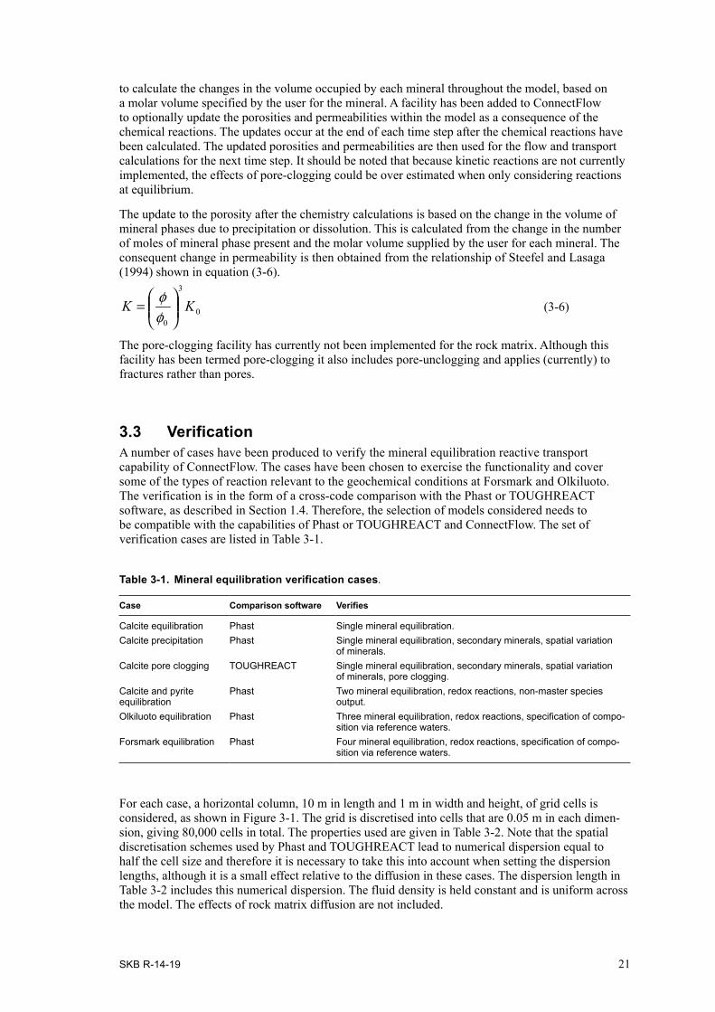
The update to the porosity after the chemistry calculations is based on the change in the volume of mineral phases due to precipitation or dissolution. This is calculated from the change in the number of moles of mineral phase present and the molar volume supplied by the user for each mineral. The consequent change in permeability is then obtained from the relationship of Steefel and Lasaga (1994) shown in equation (3-6).

0

3

0

KK

=

φφ

(3-6)

The pore-clogging facility has currently not been implemented for the rock matrix. Although this facility has been termed pore-clogging it also includes pore-unclogging and applies (currently) to fractures rather than pores.

3.3 VerificationA number of cases have been produced to verify the mineral equilibration reactive transport capability of ConnectFlow. The cases have been chosen to exercise the functionality and cover some of the types of reaction relevant to the geochemical conditions at Forsmark and Olkiluoto. The verification is in the form of a cross-code comparison with the Phast or TOUGHREACT software, as described in Section 1.4. Therefore, the selection of models considered needs to be compatible with the capabilities of Phast or TOUGHREACT and ConnectFlow. The set of verification cases are listed in Table 3-1.

Table 3-1. Mineral equilibration verification cases.

Case Comparison software Verifies

Calcite equilibration Phast Single mineral equilibration.Calcite precipitation Phast Single mineral equilibration, secondary minerals, spatial variation

of minerals.Calcite pore clogging TOUGHREACT Single mineral equilibration, secondary minerals, spatial variation

of minerals, pore clogging.Calcite and pyrite equilibration

Phast Two mineral equilibration, redox reactions, non-master species output.

Olkiluoto equilibration Phast Three mineral equilibration, redox reactions, specification of compo-sition via reference waters.

Forsmark equilibration Phast Four mineral equilibration, redox reactions, specification of compo-sition via reference waters.

For each case, a horizontal column, 10 m in length and 1 m in width and height, of grid cells is considered, as shown in Figure 3-1. The grid is discretised into cells that are 0.05 m in each dimen-sion, giving 80,000 cells in total. The properties used are given in Table 3-2. Note that the spatial discretisation schemes used by Phast and TOUGHREACT lead to numerical dispersion equal to half the cell size and therefore it is necessary to take this into account when setting the dispersion lengths, although it is a small effect relative to the diffusion in these cases. The dispersion length in Table 3-2 includes this numerical dispersion. The fluid density is held constant and is uniform across the model. The effects of rock matrix diffusion are not included.

22 SKB R-14-19

The column is initially filled with a water (aqueous solution) in equilibrium with one or more mineral phases. Then, a second water with a different composition is introduced at the upstream end of the column and allowed to flow advectively into it. The flow is specified as a flux boundary condition at the inflow end of the model and a zero pressure boundary condition at the outflow end, which also has an outflow (zero dispersive flux) boundary condition to allow the solutes to flow advectively from the model. The advective transport velocity is 0.1 m/y and the simulation is run for 120 years, allowing more than sufficient time for the incoming water to be advectively transported along the full length of the column, although dispersion and diffusion processes will cause some spreading out of the front. All concentrations are represented as mass fractions in kilograms per kilogram of solution (kg/kgs).

Table 3-2. Properties for mineral equilibration reactive transport verification.

Property Value

Permeability 1.0∙10–17 m2

Porosity 1.0∙10–4

Solute diffusion coefficient 1.0∙10–9 m2/sSolute dispersion length 0.05 mTemperature 25°C (15°C for the Forsmark and Olkiluoto equilibration cases)Fluid viscosity 1.0∙10–3 Pa/sFluid density 1.0∙103 kg/m3

Darcy flux 3.17∙10–13 m/s (1.0∙10–5 m/y)Time step size 3.157∙107 s (1.0 y)Number of time steps 120

3.3.1 Calcite equilibrationThis case considers equilibration of a mixture of a dilute glacial-type water and a sea-type water with calcite. Equilibration with calcite is one of the most common geochemical reactions and is relatively simple. The reaction is the dissolution or precipitation of calcite in equilibrium with calcium, bicarbonate and carbonate ions in aqueous solution (for the pH ranges of interest: 6 to 10). The relative propor-tions of bicarbonate and carbonate in solution will depend on the pH. The key reactions are

−+ +→← 23

23 COCaCaCO (3-7)

−+ +→← 233 COHHCO (3-8)

Equilibration with CO2(g) has not been considered. The composition of the waters is given in Table 3-3. The calcite is present in the model with a sufficient initial quantity (10.0 mol/kgw) such that it will not be depleted. The column is initially filled with the sea water in equilibrium with calcite, and the glacial water is introduced to the upstream end. Both waters are charge balanced by adjusting the chloride mass fraction and pre-equilibrated with calcite, i.e. they are individually reacted prior to mixing and reaction within the model. The standard phreeqc.dat thermodynamic database is used.

Figure 3‑1. The column model used for verification of reactive transport in ConnectFlow, coloured by head.

SKB R-14-19 23

Table 3-3. Reference water composition for the calcite equilibration case.

Glacial water Sea water

pH 9.66 7.94pe –6.54 –4.41

Component mass fractions (kg/kgs)C 3.00∙10–6 2.00∙10–5

Ca 1.00∙10–5 6.67∙10–5

Cl 2.00∙10–7 4.00∙10–3

Na 1.30∙10–7 2.59∙10–3

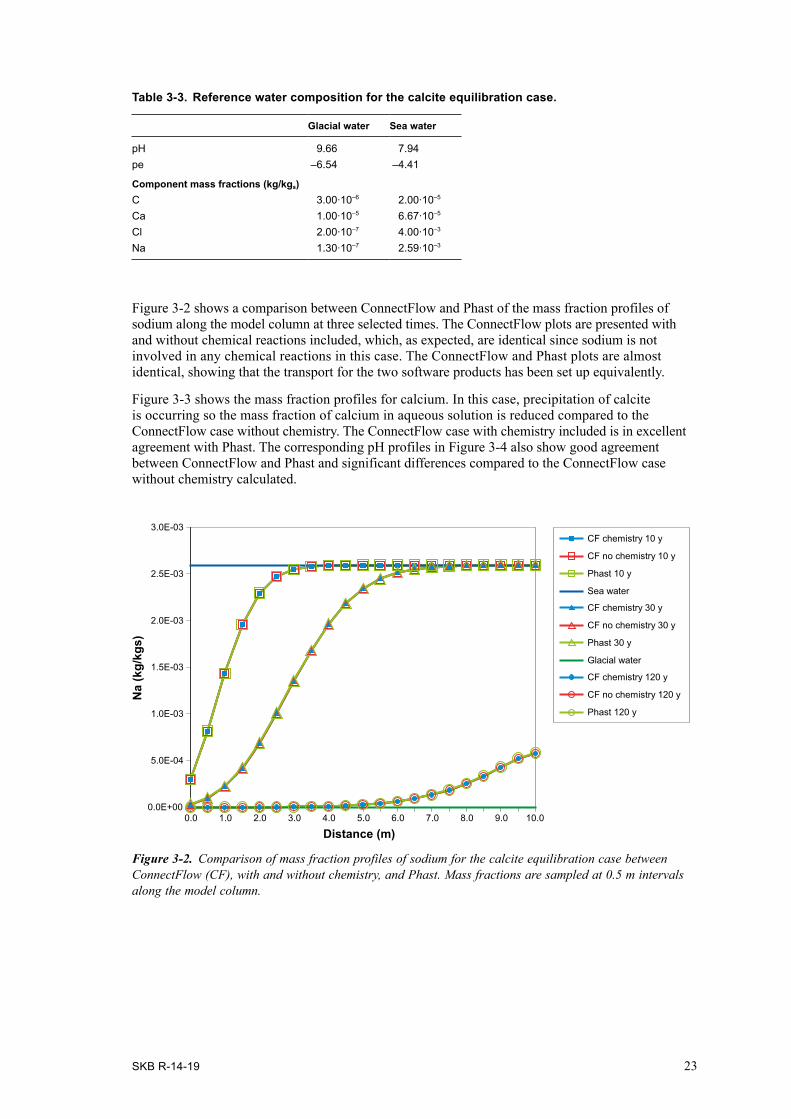
Figure 3-2 shows a comparison between ConnectFlow and Phast of the mass fraction profiles of sodium along the model column at three selected times. The ConnectFlow plots are presented with and without chemical reactions included, which, as expected, are identical since sodium is not involved in any chemical reactions in this case. The ConnectFlow and Phast plots are almost identical, showing that the transport for the two software products has been set up equivalently.

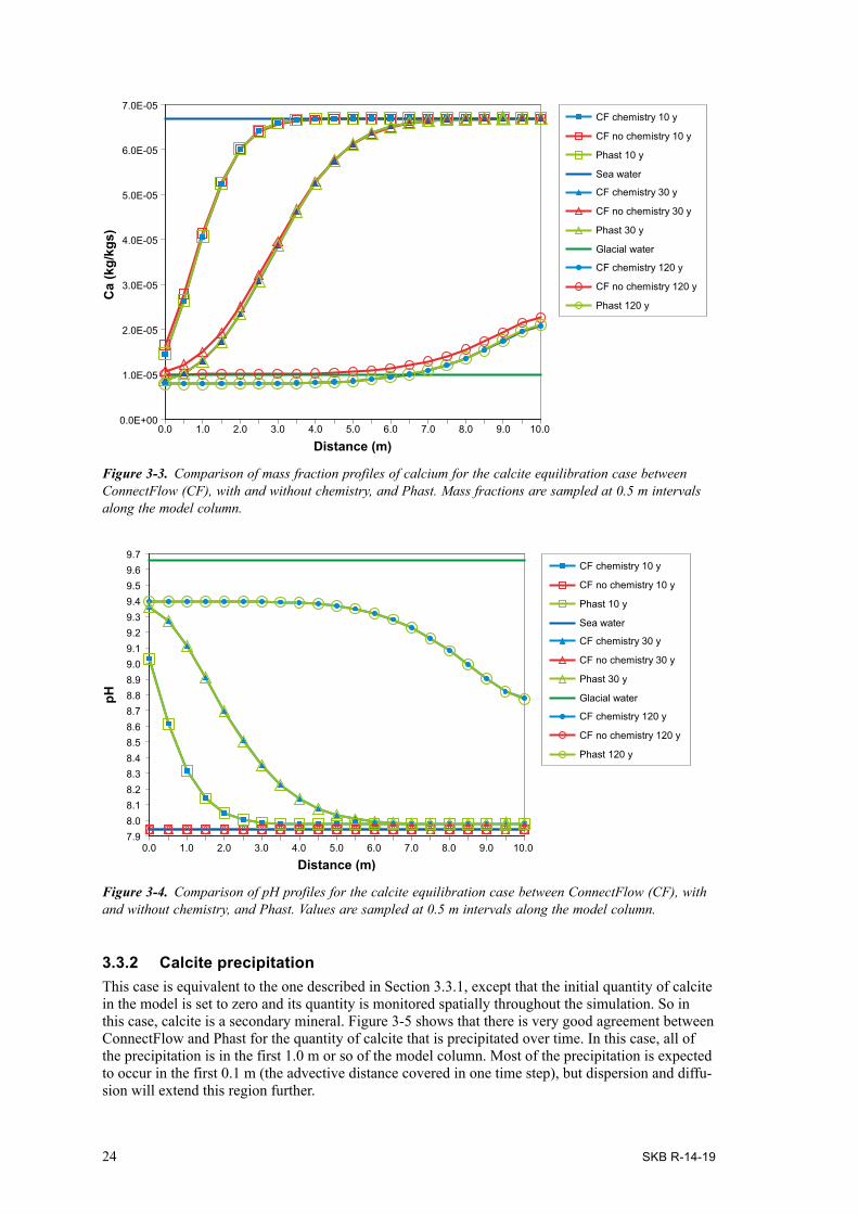
Figure 3-3 shows the mass fraction profiles for calcium. In this case, precipitation of calcite is occurring so the mass fraction of calcium in aqueous solution is reduced compared to the ConnectFlow case without chemistry. The ConnectFlow case with chemistry included is in excellent agreement with Phast. The corresponding pH profiles in Figure 3-4 also show good agreement between ConnectFlow and Phast and significant differences compared to the ConnectFlow case without chemistry calculated.

Figure 3‑2. Comparison of mass fraction profiles of sodium for the calcite equilibration case between ConnectFlow (CF), with and without chemistry, and Phast. Mass fractions are sampled at 0.5 m intervals along the model column.

0.0E+00

5.0E-04

1.0E-03

1.5E-03

2.0E-03

2.5E-03

3.0E-03

0.0 1.0 2.0 3.0 4.0 5.0 6.0 7.0 8.0 9.0 10.0

Distance (m)

Na

(kg/

kgs)

CF chemistry 120 y

CF no chemistry 120 y

Phast 120 y

CF chemistry 10 y


Phast 10 y

Sea water

CF chemistry 30 y


Phast 30 y

Glacial water

24 SKB R-14-19

Figure 3‑3. Comparison of mass fraction profiles of calcium for the calcite equilibration case between ConnectFlow (CF), with and without chemistry, and Phast. Mass fractions are sampled at 0.5 m intervals along the model column.

Figure 3‑4. Comparison of pH profiles for the calcite equilibration case between ConnectFlow (CF), with and without chemistry, and Phast. Values are sampled at 0.5 m intervals along the model column.

0.0E+00

1.0E-05

2.0E-05

3.0E-05

4.0E-05

5.0E-05

6.0E-05

7.0E-05

0.0 1.0 2.0 3.0 4.0 5.0 6.0 7.0 8.0 9.0 10.0

Distance (m)

Ca

(kg/

kgs)

CF chemistry 120 y


Phast 120 y

CF chemistry 10 y


Phast 10 y

Sea water

CF chemistry 30 y


Phast 30 y

Glacial water

CF chemistry 120 y


Phast 120 y

CF chemistry 10 y


Phast 10 y

Sea water

CF chemistry 30 y


Phast 30 y

Glacial water

7.98.08.18.28.38.48.58.68.78.88.99.09.19.29.39.49.59.69.7

0.0 1.0 2.0 3.0 4.0 5.0 6.0 7.0 8.0 9.0 10.0

pH

Distance (m)

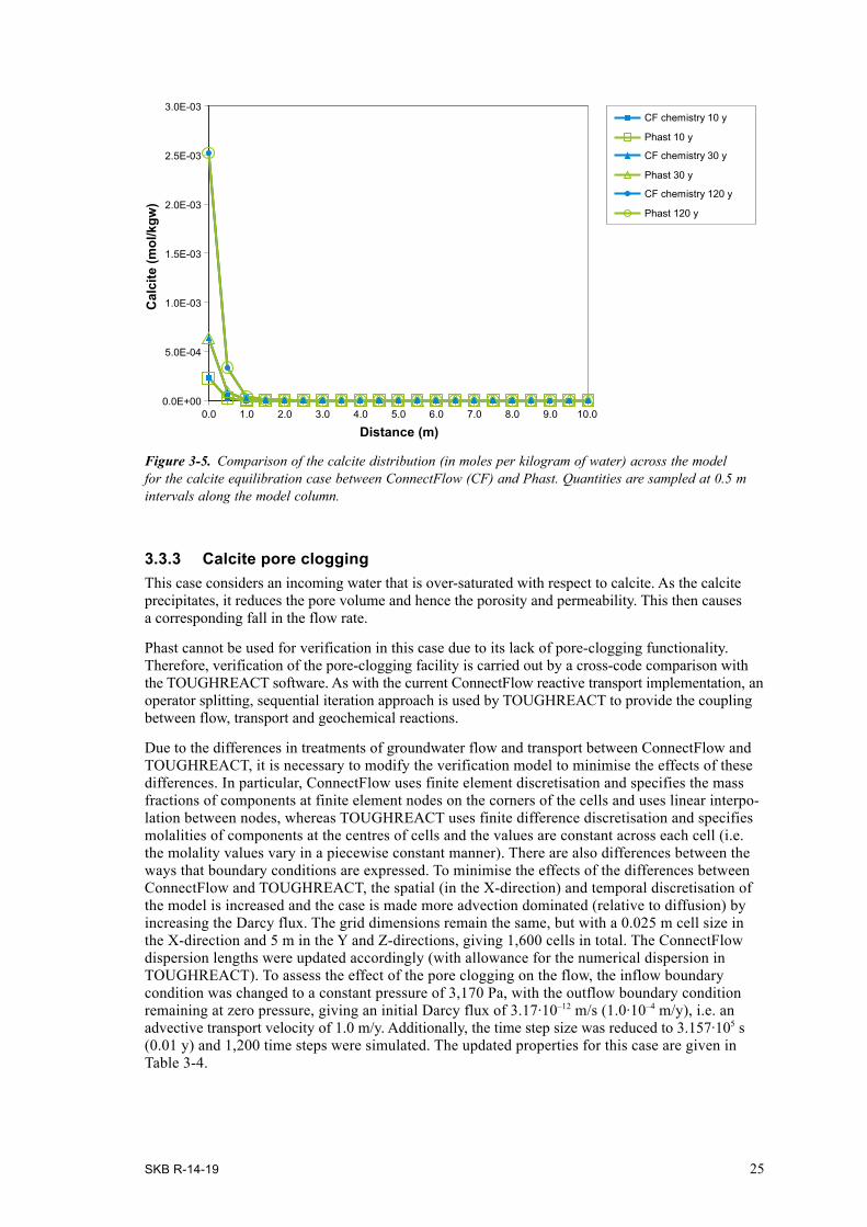
3.3.2 Calcite precipitationThis case is equivalent to the one described in Section 3.3.1, except that the initial quantity of calcite in the model is set to zero and its quantity is monitored spatially throughout the simulation. So in this case, calcite is a secondary mineral. Figure 3-5 shows that there is very good agreement between ConnectFlow and Phast for the quantity of calcite that is precipitated over time. In this case, all of the precipitation is in the first 1.0 m or so of the model column. Most of the precipitation is expected to occur in the first 0.1 m (the advective distance covered in one time step), but dispersion and diffu-sion will extend this region further.

SKB R-14-19 25

3.3.3 Calcite pore cloggingThis case considers an incoming water that is over-saturated with respect to calcite. As the calcite precipitates, it reduces the pore volume and hence the porosity and permeability. This then causes a corresponding fall in the flow rate.

Phast cannot be used for verification in this case due to its lack of pore-clogging functionality. Therefore, verification of the pore-clogging facility is carried out by a cross-code comparison with the TOUGHREACT software. As with the current ConnectFlow reactive transport implementation, an operator splitting, sequential iteration approach is used by TOUGHREACT to provide the coupling between flow, transport and geochemical reactions.

Due to the differences in treatments of groundwater flow and transport between ConnectFlow and TOUGHREACT, it is necessary to modify the verification model to minimise the effects of these differences. In particular, ConnectFlow uses finite element discretisation and specifies the mass fractions of components at finite element nodes on the corners of the cells and uses linear interpo-lation between nodes, whereas TOUGHREACT uses finite difference discretisation and specifies molalities of components at the centres of cells and the values are constant across each cell (i.e. the molality values vary in a piecewise constant manner). There are also differences between the ways that boundary conditions are expressed. To minimise the effects of the differences between ConnectFlow and TOUGHREACT, the spatial (in the X-direction) and temporal discretisation of the model is increased and the case is made more advection dominated (relative to diffusion) by increasing the Darcy flux. The grid dimensions remain the same, but with a 0.025 m cell size in the X-direction and 5 m in the Y and Z-directions, giving 1,600 cells in total. The ConnectFlow dispersion lengths were updated accordingly (with allowance for the numerical dispersion in TOUGHREACT). To assess the effect of the pore clogging on the flow, the inflow boundary condition was changed to a constant pressure of 3,170 Pa, with the outflow boundary condition remaining at zero pressure, giving an initial Darcy flux of 3.17∙10–12 m/s (1.0∙10–4 m/y), i.e. an advective transport velocity of 1.0 m/y. Additionally, the time step size was reduced to 3.157∙105 s (0.01 y) and 1,200 time steps were simulated. The updated properties for this case are given in Table 3-4.

Figure 3‑5. Comparison of the calcite distribution (in moles per kilogram of water) across the model for the calcite equilibration case between ConnectFlow (CF) and Phast. Quantities are sampled at 0.5 m intervals along the model column.

CF chemistry 120 y

Phast 120 y

CF chemistry 10 y

Phast 10 y

CF chemistry 30 y

Phast 30 y

0.0E+00

5.0E-04

1.0E-03

1.5E-03

2.0E-03

2.5E-03

3.0E-03

0.0 1.0 2.0 3.0 4.0 5.0 6.0 7.0 8.0 9.0 10.0

Cal

cite

(mol

/kgw

)

Distance (m)

26 SKB R-14-19

The chemical reaction considered is the simple precipitation of calcite, as described in Sections 3.3.1 and 3.3.2. Initially there is no calcite in the model column. The composition of the waters is given in Table 3-5. The column is initially filled with the dilute water and the over-saturated water is introduced at the upstream end. Both waters are charge balanced by adjusting the carbon mass fraction, but they are not pre-reacted. The thermodynamic database is the “Nagra/PSI Chemical Thermodynamic Data Base Version 01/01 (Nagra/PSI TDB 01/01)”, which is available in both PHREEQC and TOUGHREACT formats.

Table 3-5. Reference water composition for the calcite equilibration case.

Over-saturated water Dilute water

pH 8.00 7.00pe 4.00 4.00

Component mass fractions (kg/kgs)C 2.40∙10–3 0.00Ca 4.01∙10–3 0.00Cl 3.55∙10–5 3.55∙10–9

Na 2.30∙10–5 2.30∙10–9

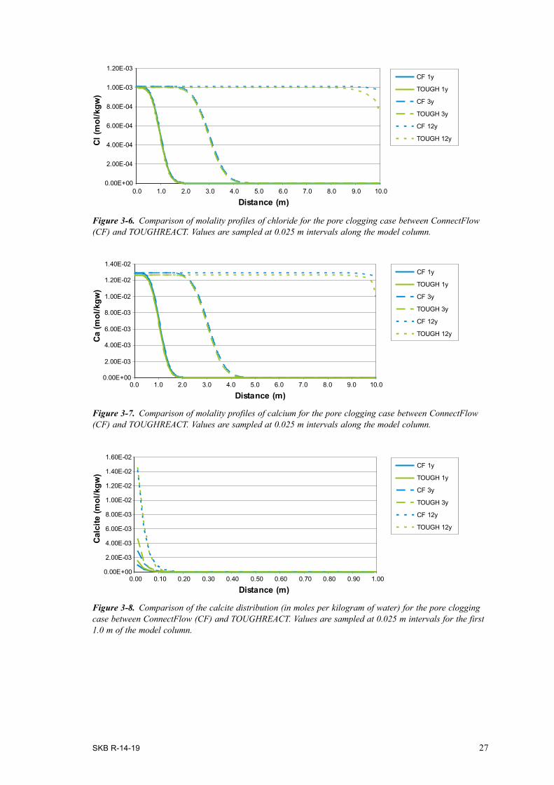
Figure 3-6 shows a comparison between the results from ConnectFlow and TOUGHREACT for the molality profiles of chloride (a non-reacting component) along the model column at three times. The plots show good agreement, except at the outflow boundary for the final time. This difference is due to differences in the way that ConnectFlow and TOUGHREACT represent outflow boundary conditions. ConnectFlow uses a zero dispersive flux boundary condition that allows solutes to flow advectively from the model. TOUGHREACT uses a very large volume boundary cell with a fixed composition to achieve a similar effect, but, in contrast to ConnectFlow, this allows diffusion of solute across the boundary. Figure 3-7 shows the corresponding comparison of molality profiles for calcium (a reactive component). There is a similar level of agreement as for chloride.

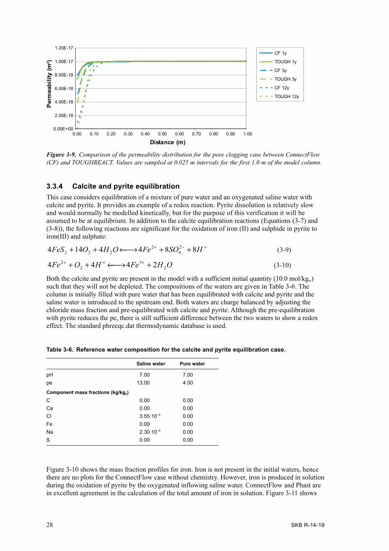
Figure 3-8 shows a comparison of the amount of calcite present in the model at three different times. Note that most of the calcite is precipitated close to the upstream end of the model (due to the oversaturation with respect to calcite, which causes precipitation in the first cell) and so the distance axis of the plots has been reduced to the range 0.0 m to 1.0 m to facilitate a more detailed comparison. There is reasonable agreement between ConnectFlow and TOUGHREACT, although there is a difference at the upstream boundary for the first two times shown. Again, this difference is due to the differences in how the boundary conditions are handled by the two software products. Figure 3-9 shows the permeability values resulting from the change in the amount of calcite with time. The agreement is reasonable between ConnectFlow and TOUGHREACT, with the differences arising due to the differences in the amount of calcite precipitated.

Table 3-4. Properties for pore-clogging reactive transport verification.

Property Value


Porosity 1.0∙10–4

Solute diffusion coefficient 1.0∙10–9 m2/sSolute dispersion length 0.0125 mTemperature 25°CFluid viscosity 1.0∙10–3 Pa/sFluid density 1.0∙103 kg/m3

Darcy flux 3.17∙10–12 m/s (1.0∙10–4 m/y)Time step size 3.157∙105 s (0.01 y)Number of time steps 1,200Molar volume of calcite 3.69∙10–5 mol/ m3

SKB R-14-19 27

0.00E+00

2.00E-04

4.00E-04

6.00E-04

8.00E-04

1.00E-03

1.20E-03

0.0 1.0 2.0 3.0 4.0 5.0 6.0 7.0 8.0 9.0 10.0

Distance (m)

Cl (m

ol/k

gw)

CF 1y

CF 3y

CF 12y

TOUGH 1y

TOUGH 3y

TOUGH 12y

Figure 3‑6. Comparison of molality profiles of chloride for the pore clogging case between ConnectFlow (CF) and TOUGHREACT. Values are sampled at 0.025 m intervals along the model column.

Figure 3‑7. Comparison of molality profiles of calcium for the pore clogging case between ConnectFlow (CF) and TOUGHREACT. Values are sampled at 0.025 m intervals along the model column.

Figure 3‑8. Comparison of the calcite distribution (in moles per kilogram of water) for the pore clogging case between ConnectFlow (CF) and TOUGHREACT. Values are sampled at 0.025 m intervals for the first 1.0 m of the model column.

CF 1y

CF 3y

CF 12y

TOUGH 1y

TOUGH 3y

TOUGH 12y

0.00E+00

2.00E-03

4.00E-03

6.00E-03

8.00E-03

1.00E-02

1.20E-02

1.40E-02

0.0 1.0 2.0 3.0 4.0 5.0 6.0 7.0 8.0 9.0 10.0

Distance (m)

Ca (m

ol/k

gw)

CF 1y

CF 3y

CF 12y

TOUGH 1y

TOUGH 3y

TOUGH 12y

0.00E+00

2.00E-03

4.00E-03

6.00E-03

8.00E-03

1.00E-02

1.20E-02

1.40E-02

1.60E-02

0.00 0.10 0.20 0.30 0.40 0.50 0.60 0.70 0.80 0.90 1.00

Distance (m)

Calc

ite (m

ol/k

gw)

28 SKB R-14-19

3.3.4 Calcite and pyrite equilibrationThis case considers equilibration of a mixture of pure water and an oxygenated saline water with calcite and pyrite. It provides an example of a redox reaction. Pyrite dissolution is relatively slow and would normally be modelled kinetically, but for the purpose of this verification it will be assumed to be at equilibrium. In addition to the calcite equilibration reactions (Equations (3-7) and (3-8)), the following reactions are significant for the oxidation of iron (II) and sulphide in pyrite to iron(III) and sulphate:

+−+ ++→←++ HSOFeOHOFeS 8844144 24

2222 (3-9)

OHFeHOFe 23

22 2444 +→←++ +++

(3-10)

Both the calcite and pyrite are present in the model with a sufficient initial quantity (10.0 mol/kgw) such that they will not be depleted. The compositions of the waters are given in Table 3-6. The column is initially filled with pure water that has been equilibrated with calcite and pyrite and the saline water is introduced to the upstream end. Both waters are charge balanced by adjusting the chloride mass fraction and pre-equilibrated with calcite and pyrite. Although the pre-equilibration with pyrite reduces the pe, there is still sufficient difference between the two waters to show a redox effect. The standard phreeqc.dat thermodynamic database is used.

Table 3-6. Reference water composition for the calcite and pyrite equilibration case.

Saline water Pure water

pH 7.00 7.00pe 13.00 4.00

Component mass fractions (kg/kgs)C 0.00 0.00Ca 0.00 0.00Cl 3.55∙10–5 0.00Fe 0.00 0.00Na 2.30∙10–5 0.00S 0.00 0.00

Figure 3-10 shows the mass fraction profiles for iron. Iron is not present in the initial waters, hence there are no plots for the ConnectFlow case without chemistry. However, iron is produced in solution during the oxidation of pyrite by the oxygenated inflowing saline water. ConnectFlow and Phast are in excellent agreement in the calculation of the total amount of iron in solution. Figure 3-11 shows

Figure 3‑9. Comparison of the permeability distribution for the pore clogging case between ConnectFlow (CF) and TOUGHREACT. Values are sampled at 0.025 m intervals for the first 1.0 m of the model column.

CF 1y

CF 3y

CF 12y

TOUGH 1y

TOUGH 3y

TOUGH 12y

0.00E+00

2.00E-18

4.00E-18

6.00E-18

8.00E-18

1.00E-17

1.20E-17

0.00 0.10 0.20 0.30 0.40 0.50 0.60 0.70 0.80 0.90 1.00

Distance (m)

Perm

eabi

lity

(m2 )

SKB R-14-19 29

the mass fraction profiles for sulphate, an example of the output of a non-master species, again showing very good agreement between Phast and ConnectFlow. They are also in good agreement for the pe values calculated (a measure of the redox conditions), as shown in Figure 3-12.

Figure 3‑10. Comparison of mass fraction profiles of iron for the calcite and pyrite equilibration case between ConnectFlow (CF) and Phast. Mass fractions are sampled at 0.5 m intervals along the model column.

Figure 3‑11. Comparison of mass fraction profiles of sulphate for the calcite and pyrite equilibration case between ConnectFlow (CF) and Phast. Mass fractions are sampled at 0.5 m intervals along the model column.

0.0E+00

2.0E-09

4.0E-09

6.0E-09

8.0E-09

1.0E-08

1.2E-08

1.4E-08

0.0 1.0 2.0 3.0 4.0 5.0 6.0 7.0 8.0 9.0 10.0

Distance (m)

Fe (k

g/kg

s)

CF chemistry 120 y

Phast 120 y

CF chemistry 10 y

Phast 10 y

CF chemistry 30 y

Phast 30 y

CF chemistry 120 y

Phast 120 y

CF chemistry 10 y

Phast 10 y

CF chemistry 30 y

Phast 30 y

0.0E+00

1.0E-08

2.0E-08

3.0E-08

4.0E-08

5.0E-08

0.0 1.0 2.0 3.0 4.0 5.0 6.0 7.0 8.0 9.0 10.0

Distance (m)

Sulp

hate

(kg/

kgs)

30 SKB R-14-19

3.3.5 Olkiluoto equilibrationThis case considers a selection of minerals, waters and reactions relevant for the Olkiluoto site. The reactions are equilibration of the Littorina and Altered Meteoric reference waters (see Section 7.2) with calcite, pyrite and quartz. The equilibration reactions for calcite and pyrite are given by Equations (3-7) to (3-10). The equation for the dissolution of quartz is

4422 2 SiOHOHSiO →←+ (3-11)

The standard phreeqc.dat thermodynamic database is used. The minerals are present in the model with a sufficient initial quantity (10.0 mol/kgw) such that they will not be depleted. The composition of the reference waters are given in Table 7-2. The model is initially filled with Littorina water and Altered Meteoric water is introduced at the upstream end.

Figure 3-13 shows the mass fraction profiles of calcium in aqueous solution for three different times. Again, Phast and ConnectFlow are in excellent agreement. It can be seen that the mass fraction of calcium is higher when chemical reactions are included, indicating that calcite is dissolving in this case. However, the mass fractions of sulphur shown in Figure 3-14 are the same with and without chemical reactions included, indicating that the pyrite is not precipitating or dissolving under these conditions. Again, ConnectFlow and Phast are in good agreement.

3.3.6 Forsmark equilibrationThis case considers a selection of minerals, waters and reactions relevant for the Forsmark site. The reactions are equilibration of the Littorina and Glacial reference waters (see Section 7.1) with calcite, quartz, hydroxyapatite and amorphous iron(II) sulphide (FeS(ppt)). The equilibration reactions for calcite are given by Equations (3-7) and (3-8) and for quartz by Equation (3-11). The equation for the dissolution of hydroxyapatite is

OHHPOCaHOHPOCa 224

2345 354)()( ++→←+ −++ (3-12)

and for FeS(ppt)−++ +→←+ HSFeHFeS 2 (3-13)

Figure 3‑12. Comparison of pe profiles for the calcite and pyrite equilibration case between ConnectFlow (CF) and Phast. Values are sampled at 0.5 m intervals along the model column.

CF chemistry 120 y

Phast 120 y

CF chemistry 10 y

Phast 10 y

CF chemistry 30 y

Phast 30 y

-6.9

-6.8

-6.7

-6.60.0 1.0 2.0 3.0 4.0 5.0 6.0 7.0 8.0 9.0 10.0

Distance (m)pe

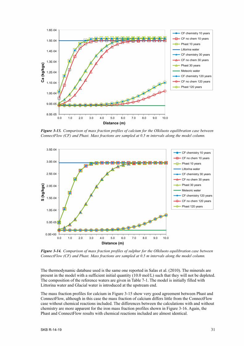
SKB R-14-19 31

CF chemistry 120 years

CF no chem 120 years

Phast 120 years


CF no chem 10 years

Phast 10 years

Littorina water


CF no chem 30 years

Phast 30 years

Meteoric water

8.0E-05

9.0E-05

1.0E-04

1.1E-04

1.2E-04

1.3E-04

1.4E-04

1.5E-04

1.6E-04

0.0 1.0 2.0 3.0 4.0 5.0 6.0 7.0 8.0 9.0 10.0

Distance (m)

Ca

(kg/

kgs)

Figure 3‑13. Comparison of mass fraction profiles of calcium for the Olkiluoto equilibration case between ConnectFlow (CF) and Phast. Mass fractions are sampled at 0.5 m intervals along the model column.

Figure 3‑14. Comparison of mass fraction profiles of sulphur for the Olkiluoto equilibration case between ConnectFlow (CF) and Phast. Mass fractions are sampled at 0.5 m intervals along the model column.



Phast 120 years


CF no chem 10 years

Phast 10 years

Littorina water


CF no chem 30 years

Phast 30 years

Meteoric water

0.0E+00

5.0E-05

1.0E-04

1.5E-04

2.0E-04

2.5E-04

3.0E-04

3.5E-04

0.0 1.0 2.0 3.0 4.0 5.0 6.0 7.0 8.0 9.0 10.0

Distance (m)

S (k

g/kg

s)

The thermodynamic database used is the same one reported in Salas et al. (2010). The minerals are present in the model with a sufficient initial quantity (10.0 mol/L) such that they will not be depleted. The composition of the reference waters are given in Table 7-1. The model is initially filled with Littorina water and Glacial water is introduced at the upstream end.

The mass fraction profiles for calcium in Figure 3-15 show very good agreement between Phast and ConnectFlow, although in this case the mass fraction of calcium differs little from the ConnectFlow case without chemical reactions included. The differences between the calculations with and without chemistry are more apparent for the iron mass fraction profiles shown in Figure 3-16. Again, the Phast and ConnectFlow results with chemical reactions included are almost identical.

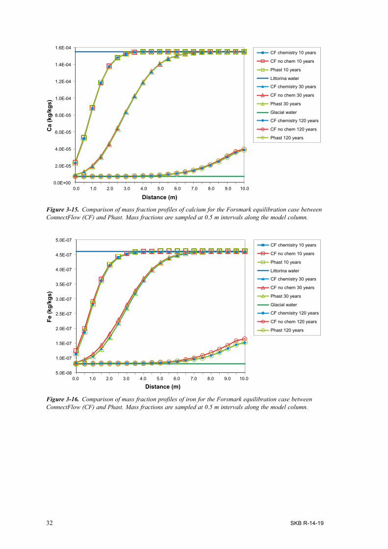
32 SKB R-14-19

Figure 3‑15. Comparison of mass fraction profiles of calcium for the Forsmark equilibration case between ConnectFlow (CF) and Phast. Mass fractions are sampled at 0.5 m intervals along the model column.

Figure 3‑16. Comparison of mass fraction profiles of iron for the Forsmark equilibration case between ConnectFlow (CF) and Phast. Mass fractions are sampled at 0.5 m intervals along the model column.

0.0E+00

2.0E-05

4.0E-05

6.0E-05

8.0E-05

1.0E-04

1.2E-04

1.4E-04

1.6E-04

0.0 1.0 2.0 3.0 4.0 5.0 6.0 7.0 8.0 9.0 10.0

Distance (m)

Ca

(kg/

kgs)



Phast 120 years


CF no chem 10 years

Phast 10 years

Littorina water


CF no chem 30 years

Phast 30 years

Glacial water

5.0E-08

1.0E-07

1.5E-07

2.0E-07

2.5E-07

3.0E-07

3.5E-07

4.0E-07

4.5E-07

5.0E-07

0.0 1.0 2.0 3.0 4.0 5.0 6.0 7.0 8.0 9.0 10.0

Distance (m)

Fe (k

g/kg

s)



Phast 120 years


CF no chem 10 years

Phast 10 years

Littorina water


CF no chem 30 years

Phast 30 years

Glacial water

SKB R-14-19 33

4 Ion exchange reactions

4.1 ContextIon exchange reactions are reversible processes that occur between ions held at the surface of a mineral and ions in aqueous solution. These reactions have implications for the water composition due to their ability to swap one ion for another in aqueous solution. Ion exchange properties are seen in some minerals, particularly clays, such as zeolites and montmorillonite. Clays occur on fracture surfaces at both Forsmark (Löfgren and Sidborn 2010) and Olkiluoto (Posiva 2009) and so there is potential for ion exchange reactions in the fractured rock at these sites. The bentonite used in reposi-tory backfill and around the radioactive waste canisters is also an ion exchanger. Although ion exchange reactions were not considered at the regional-scale for SR-Site due to a lack of data (Salas et al. 2010) they have been considered for Olkiluoto with an illite-like exchanger (Trinchero et al. 2014).

4.2 ImplementationThe capability to carry out ion exchange reactions has been implemented in ConnectFlow by provid-ing an interface to these calculations in iPhreeqc. These reactions can be carried out in conjunction with equilibration with mineral phases or can be carried out separately. The ion exchangers to be used can be selected from the master exchangers or the exchanger species present in the thermo-dynamic database used. If a master exchanger is specified then its initial state can optionally be set by equilibration with the aqueous solution present in each reaction cell. The initial quantity of each exchanger can be specified for the whole model in moles per kilogram of water, with a default value of zero if not specified. If mineral variables are used (Section 3.2.1) then a spatially varying initial quantity of each exchanger can be specified. The values associated with these variables are updated by the ion exchange reactions for user information and output, although the state of the exchangers is maintained internally by iPhreeqc and no further reference to the ConnectFlow variables is required after the initial equilibration. Exchanger species (i.e. not master exchangers) are treated as non-master species for the purposes of output from ConnectFlow (Section 2.4.9).

4.3 VerificationThe ion exchange reaction capability within ConnectFlow has been verified by comparison with Phast, as described in Section 3.3. The same model was used as in Section 3.3 with the properties listed in Table 3-2. The list of cases used to verify the ion exchange functionality is given in Table 4-1. The cases test the ion exchange capability in isolation and in conjunction with the mineral equilib-rium capability. They also test different ways of specifying the initial amount and composition of the exchanger.

Table 4-1. Ion exchange verification cases.

Case Comparison software Verifies

Ion exchange only Phast Ion exchange reactions, initial exchanger composition from equilibration with solution.

Ion exchange with mineral equilibration

Phast Ion exchange reactions with mineral equilibration, explicit initial exchanger composition, output of non-master species

34 SKB R-14-19

4.3.1 Ion exchange onlyThis case considers the reaction of a mixture of two aqueous solutions and an ion exchanger that is able to exchange cations. The reactions are defined in the standard phreeqc.dat thermodynamic database, using the example exchanger ‘X’. The model initially contains a sodium chloride (NaCl) solution, with a small amount of potassium, and a calcium chloride (CaCl2) solution is introduced at the upstream end of the column. The composition of the waters is given in Table 4-2. The column also contains the ion exchanger X with an initial quantity of 0.011 moles per kilogram of water (mol/kgw), whose composition is initialised by equilibrium with the NaCl water.

Table 4-2. Reference water composition for the ion exchange case.

CaCl2 water NaCl water

pH 7.00 7.00pe 4.00 4.00

Component mass fractions (kg/kgs)Ca 2.40∙10–4 0.00Cl 4.25∙10–4 3.90∙10–4

K 0.00 3.91∙10–5

Na 0.00 2.30∙10–4

Figure 4-1 shows the mass fraction profiles of chloride for three different times. This is a non-reactive component and there is good agreement between ConnectFlow (with and without chemistry) and Phast, showing that the transport is equivalent in each calculation. Figure 4-2 shows the mass fraction profiles for calcium. This is not present in solution initially in the model, but as it is introduced in the CaCl2 water its mass fraction rises with time. However, its mass fraction is reduced compared to the ConnectFlow case without chemistry calculations because the calcium ions are taken up by the ion exchanger, which releases sodium and potassium ions as a consequence.

Figure 4‑1. Comparison of mass fraction profiles of chloride for the ion exchange case between ConnectFlow (CF), with and without chemistry, and Phast. Mass fractions are sampled at 0.5 m intervals along the model column.

3.9E-04

4.0E-04

4.1E-04

4.2E-04

4.3E-04

0.0 1.0 2.0 3.0 4.0 5.0 6.0 7.0 8.0 9.0 10.0

Distance (m)

Cl (

kg/k

gs)

CF chemistry 120 y


Phast 120 y

CF chemistry 10 y


Phast 10 y

NaCl water

CF chemistry 30 y


Phast 30 y

CaCl2 water

SKB R-14-19 35

Figure 4-3 shows that the potassium mass fraction in solution rises as it is replaced in the ion exchanger by the calcium ions before eventually being flushed out by the CaCl2 water. The correspond-ing profiles for the exchanger species are shown in Figure 4-4 to Figure 4-6, which show the replacement of sodium and potassium by calcium on the ion exchanger. Some of the sodium seems to be replaced by potassium on the ion exchanger just before the replacement by calcium. There is excellent agreement between the results for ConnectFlow and Phast.

Figure 4‑2. Comparison of mass fraction profiles of calcium for the ion exchange case between ConnectFlow (CF), with and without chemistry, and Phast. Mass fractions are sampled at 0.5 m intervals along the model column.

Figure 4‑3. Comparison of mass fraction profiles of potassium for the ion exchange case between ConnectFlow (CF), with and without chemistry, and Phast. Mass fractions are sampled at 0.5 m intervals along the model column.

0.0E+00

5.0E-05

1.0E-04

1.5E-04

2.0E-04

2.5E-04

0.0 1.0 2.0 3.0 4.0 5.0 6.0 7.0 8.0 9.0 10.0

Distance (m)

Ca

(kg/

kgs)

CF chemistry 120 y


Phast 120 y

CF chemistry 10 y


Phast 10 y

NaCl water

CF chemistry 30 y


Phast 30 y

CaCl2 water

0.0E+00

5.0E-05

1.0E-04

1.5E-04

2.0E-04

2.5E-04

0.0 1.0 2.0 3.0 4.0 5.0 6.0 7.0 8.0 9.0 10.0

Distance (m)

K (k

g/kg

s)

CF chemistry 120 y


Phast 120 y

CF chemistry 10 y


Phast 10 y

NaCl water

CF chemistry 30 y


Phast 30 y

CaCl2 water

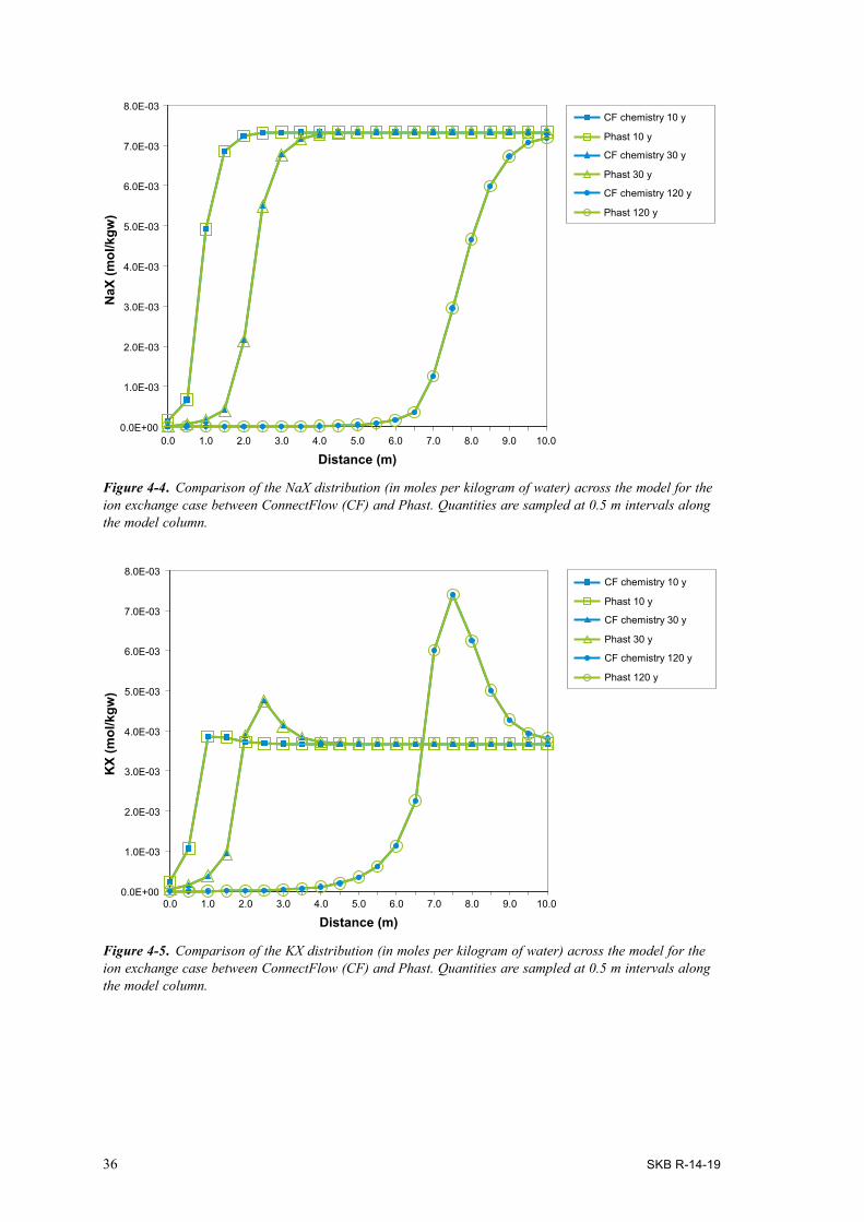
36 SKB R-14-19

Figure 4‑4. Comparison of the NaX distribution (in moles per kilogram of water) across the model for the ion exchange case between ConnectFlow (CF) and Phast. Quantities are sampled at 0.5 m intervals along the model column.

Figure 4‑5. Comparison of the KX distribution (in moles per kilogram of water) across the model for the ion exchange case between ConnectFlow (CF) and Phast. Quantities are sampled at 0.5 m intervals along the model column.

0.0E+00

1.0E-03

2.0E-03

3.0E-03

4.0E-03

5.0E-03

6.0E-03

7.0E-03

8.0E-03

0.0 1.0 2.0 3.0 4.0 5.0 6.0 7.0 8.0 9.0 10.0

Distance (m)

NaX

(mol

/kgw

)

CF chemistry 120 y

Phast 120 y

CF chemistry 10 y

Phast 10 y

CF chemistry 30 y

Phast 30 y

0.0E+00

1.0E-03

2.0E-03

3.0E-03

4.0E-03

5.0E-03

6.0E-03

7.0E-03

8.0E-03

0.0 1.0 2.0 3.0 4.0 5.0 6.0 7.0 8.0 9.0 10.0

Distance (m)

KX

(mol

/kgw

)

CF chemistry 120 y

Phast 120 y

CF chemistry 10 y

Phast 10 y

CF chemistry 30 y

Phast 30 y

SKB R-14-19 37

4.3.2 Ion exchange with mineral equilibrationThis case considers the reaction of a mixture of two aqueous solutions in equilibrium with a mineral phase and an ion exchanger that is able to exchange cations. The reactions are defined in the standard phreeqc.dat thermodynamic database, using the example exchanger ‘X’. The model initially contains a sodium chloride (NaCl) solution, with a small amount of potassium and bicarbonate, and a calcium chloride (CaCl2) solution is introduced at the upstream end of the column. The composition of the waters is given in Table 4-3. The column also contains an ion exchanger X with an initial quantity of 0.011 mol/kgw, whose initial composition is defined as fully NaX. There is also 1.0 mol/kgw of calcite present in the column initially.

Figure 4‑6. Comparison of the CaX2 distribution (in moles per kilogram of water) across the model for the ion exchange case between ConnectFlow (CF) and Phast. Quantities are sampled at 0.5 m intervals along the model column.

Table 4-3. Reference water composition for the ion exchange with mineral equilibration case.

CaCl2 water NaCl water

pH 7.00 7.00pe 4.00 4.00

Component mass fractions (kg/kgs)C 0.00 1.20∙10–5

Ca 2.40∙10–4 0.00Cl 4.25∙10–4 3.25∙10–4

K 0.00 3.91∙10–5

Na 0.00 2.07∙10–4

0.0E+00

1.0E-03

2.0E-03

3.0E-03

4.0E-03

5.0E-03

6.0E-03

0.0 1.0 2.0 3.0 4.0 5.0 6.0 7.0 8.0 9.0 10.0

Distance (m)

CaX

2 (m

ol/k

gw)

CF chemistry 120 y

Phast 120 y

CF chemistry 10 y

Phast 10 y

CF chemistry 30 y

Phast 30 y

Figure 4-7 shows that the transport for ConnectFlow (with and without chemistry) and Phast is equivalent for the non-reacting chloride component. Figure 4-8 shows excellent agreement between the mass fraction profiles of calcium for Phast and ConnectFlow. It can be seen that the calcium mass fraction in solution is considerably reduced when chemical reactions are included. This is predominantly due to take up of calcium by the ion exchanger rather than due to precipitation of calcite, since Figure 4-8 is very similar to Figure 4-2, which does not include calcite equilibration.

38 SKB R-14-19

Figure 4-9 shows the mass fraction profiles for sodium ions. Again, the ConnectFlow results with chemistry are in excellent agreement with the Phast results. In this case the sodium mass fractions in solution are higher when chemical reactions are included, caused by the release of sodium ions from the exchanger due to replacement by calcium. The distributions of NaX, KX and CaX2 across the model for three different times, given in Figure 4-10 to Figure 4-12 respectively, show the replace-ment of sodium and potassium by calcium on the ion exchanger.

Figure 4‑7. Comparison of mass fraction profiles of chloride for the ion exchange with mineral equilibra-tion case between ConnectFlow (CF), with and without chemistry, and Phast. Mass fractions are sampled at 0.5 m intervals along the model column.

Figure 4‑8. Comparison of mass fraction profiles of calcium for the ion exchange with mineral equilibra-tion case between ConnectFlow (CF), with and without chemistry, and Phast. Mass fractions are sampled at 0.5 m intervals along the model column.

3.2E-04

3.4E-04

3.6E-04

3.8E-04

4.0E-04

4.2E-04

0.0 1.0 2.0 3.0 4.0 5.0 6.0 7.0 8.0 9.0 10.0

Distance (m)

Cl (

kg/k

gs)

CF chemistry 120 y


Phast 120 y

CF chemistry 10 y


Phast 10 y

NaCl water

CF chemistry 30 y


Phast 30 y

CaCl2 water

0.0E+00

5.0E-05

1.0E-04

1.5E-04

2.0E-04

2.5E-04

0.0 1.0 2.0 3.0 4.0 5.0 6.0 7.0 8.0 9.0 10.0

Distance (m)

Ca

(kg/

kgs)

CF chemistry 120 y


Phast 120 y

CF chemistry 10 y


Phast 10 y

NaCl water

CF chemistry 30 y


Phast 30 y

CaCl2 water

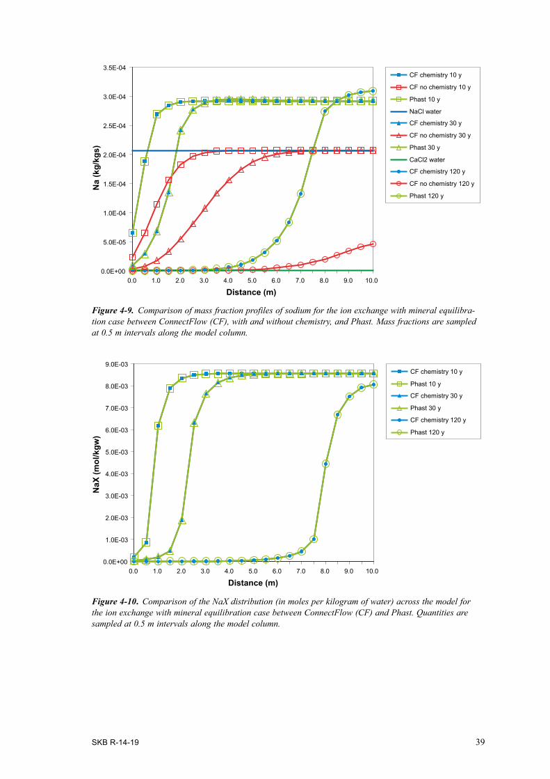
SKB R-14-19 39

Figure 4‑9. Comparison of mass fraction profiles of sodium for the ion exchange with mineral equilibra-tion case between ConnectFlow (CF), with and without chemistry, and Phast. Mass fractions are sampled at 0.5 m intervals along the model column.

Figure 4‑10. Comparison of the NaX distribution (in moles per kilogram of water) across the model for the ion exchange with mineral equilibration case between ConnectFlow (CF) and Phast. Quantities are sampled at 0.5 m intervals along the model column.

0.0E+00

1.0E-03

2.0E-03

3.0E-03

4.0E-03

5.0E-03

6.0E-03

7.0E-03

8.0E-03

9.0E-03

0.0 1.0 2.0 3.0 4.0 5.0 6.0 7.0 8.0 9.0 10.0

Distance (m)

NaX

(mol

/kgw

)

CF chemistry 120 y

Phast 120 y

CF chemistry 10 y

Phast 10 y

CF chemistry 30 y

Phast 30 y

0.0E+00

5.0E-05

1.0E-04

1.5E-04

2.0E-04

2.5E-04

3.0E-04

3.5E-04

0.0 1.0 2.0 3.0 4.0 5.0 6.0 7.0 8.0 9.0 10.0

Distance (m)

Na

(kg/

kgs)

CF chemistry 120 y


Phast 120 y

CF chemistry 10 y


Phast 10 y

NaCl water

CF chemistry 30 y


Phast 30 y

CaCl2 water

40 SKB R-14-19

Figure 4‑11. Comparison of the KX distribution (in moles per kilogram of water) across the model for the ion exchange with mineral equilibration case between ConnectFlow (CF) and Phast. Quantities are sampled at 0.5 m intervals along the model column.

Figure 4‑12. Comparison of the CaX2 distribution (in moles per kilogram of water) across the model for the ion exchange with mineral equilibration case between ConnectFlow (CF) and Phast. Quantities are sampled at 0.5 m intervals along the model column.

0.0E+00

1.0E-03

2.0E-03

3.0E-03

4.0E-03

5.0E-03

6.0E-03

0.0 1.0 2.0 3.0 4.0 5.0 6.0 7.0 8.0 9.0 10.0

Distance (m)

CaX

2(mol

/kgw

) CF chemistry 120 y

Phast 120 y

CF chemistry 10 y

Phast 10 y

CF chemistry 30 y

Phast 30 y

0.0E+00

5.0E-05

1.0E-04

1.5E-04

2.0E-04

2.5E-04

3.0E-04

3.5E-04

0.0 1.0 2.0 3.0 4.0 5.0 6.0 7.0 8.0 9.0 10.0

Distance (m)

KX

(mol

/kgw

)

CF chemistry 120 y

Phast 120 y

CF chemistry 10 y

Phast 10 y

CF chemistry 30 y

Phast 30 y

SKB R-14-19 41

5 Rock matrix diffusion

5.1 IntroductionThe original method of rock matrix diffusion in ConnectFlow (Hoch and Jackson 2004) uses an analytic solution to describe the flux between the fracture and the rock matrix. This method has been used for the site descriptive modelling of Forsmark (Follin 2008) and Olkiluoto (Hartley et al. 2012) and in SR-Site (Joyce et al. 2010). The analytic solution that underpins the method only represents diffusion in the rock matrix and is not applicable if chemical reactions are occurring. To deal with this issue, a new method to calculate rock matrix diffusion has been implemented based on a finite volume approach.

5.2 Finite volume rock matrix diffusionA finite volume rock matrix diffusion method has been implemented to allow the effects of rock matrix diffusion to be modelled in situations where chemical reactions are being calculated. This method may also be used where no chemical reactions are being calculated. The original method of RMD is still available in ConnectFlow, the equations for which are given in Section 2.3.

The original RMD method uses an expression for the flux into the rock matrix derived from an analytic model. The new method models the diffusion of solutes between cells in the rock matrix using a finite volume method. The flux between the fracture and matrix can then be calculated. This new method more readily provides a detailed description of the distribution of solutes within the rock matrix. It is also straightforward to generalise the approach to handle chemical reactions in the rock matrix. A simplified schematic of the two methods is shown in Figure 5-1. With the new method, the user selects the number of cells that the rock matrix is divided up into per fractured rock finite element and also may choose if these are to be of equal length or have varying lengths. As changes in matrix water composition due to diffusion are greatest closest to the fracture, smaller cell sizes for the first few matrix cells may improve accuracy, whilst larger cell sizes for the other matrix cells will help performance without a significant reduction in accuracy.

Figure 5‑1. Simplified schematic of the original and finite volume rock matrix diffusion methods. The blue arrows show flow within the fractures, the large black arrows show flow between the fractures and the rock matrix, and the small black arrows show flow within the rock matrix.

Finite volume RMD

Rock matrixFractureRock matrixFracture

Original RMD

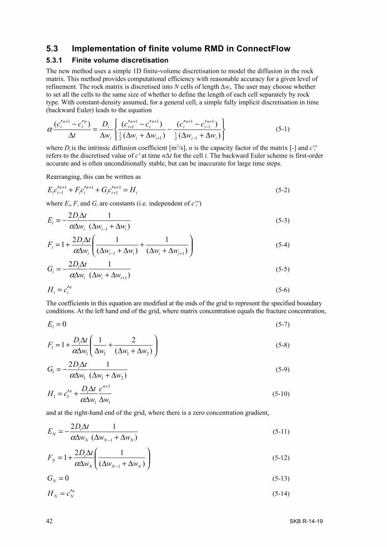
42 SKB R-14-19

5.3 Implementation of finite volume RMD in ConnectFlow5.3.1 Finite volume discretisationThe new method uses a simple 1D finite-volume discretisation to model the diffusion in the rock matrix. This method provides computational efficiency with reasonable accuracy for a given level of refinement. The rock matrix is discretised into N cells of length Δwi. The user may choose whether to set all the cells to the same size of whether to define the length of each cell separately by rock type. With constant-density assumed, for a general cell, a simple fully implicit discretisation in time (backward Euler) leads to the equation

∆+∆′-′

-∆+∆′-′

∆=

∆′-′

-

+-

+

+

+++

+

)()(

)()()(

121

11

1

121

111

1

ii

ni

ni

ii

ni

ni

i

in

in

i

wwcc

wwcc

wD

tccα (5-1)

where Di is the intrinsic diffusion coefficient [m2/s], α is the capacity factor of the matrix [-] and c'in refers to the discretised value of c' at time nΔt for the cell i. The backward Euler scheme is first-order accurate and is often unconditionally stable, but can be inaccurate for large time steps.

Rearranging, this can be written as

in

iin

iin

ii HcGcFcE =′+′+′ ++

++-

11

111 (5-2)

where Ei, Fi and Gi are constants (i.e. independent of c'in)

)(12

1 iii

ii www

tDE∆+∆∆

∆-=-α

(5-3)

∆+∆

+∆+∆∆

∆+=+- )(

1)(

12111 iiiii

ii wwwww

tDFα

(5-4)

)(12

1+∆+∆∆∆-=

iii

ii www

tDGα

(5-5)

nii cH ′= (5-6)

The coefficients in this equation are modified at the ends of the grid to represent the specified boundary conditions. At the left hand end of the grid, where matrix concentration equals the fracture concentration,

01 =E (5-7)

∆+∆

+∆∆

∆+=)(

2112111

1 wwwwtDF i

α (5-8)

)(12

2111 www

tDG i

∆+∆∆∆-=

α (5-9)

1

1

111 w

cwtDcH

nin

∆∆∆+′=

+

α (5-10)

and at the right-hand end of the grid, where there is a zero concentration gradient,

)(12

1 NNN

iN www

tDE∆+∆∆

∆-=-α

(5-11)

∆+∆∆

∆+=- )(

1211 NNN

iN www

tDFα

(5-12)

0=NG (5-13)

nNN cH ′= (5-14)

SKB R-14-19 43

The discretised equations form a tridiagonal system, which can be readily solved using the Thomas algorithm (Thomas 1949).

The case of interest is slightly more complicated than this because the equations involve the unknown c, which is the value of the solute mass fraction in the fracture system at the end of the time step. However, this can be readily handled as follows. Equation (5-2) can be written in the form

in

in

iin

iin

ii HCHcGcFcE 21 111

111

+++

++- +=′+′+′ (5-15)

where, from Equation (5-6) and Equation (5-10),n

ii cH ′=1 (5-16)

and

=

∆∆∆

=else

iww

tDH

i

i

0

112 11α (5-17)

Equation (5-15) is a linear equation for c' n+1 and so the solution is given by 1

,211

,11 ++++ ′+′=′ n

inn

in

i cccc (5-18)

where c'1,in+1 and c'2,i

n+ are the solutions of the linear system for right-hand sides H1i and H2i respectively, i.e.

inii

nii

nii HcGcFcE 11

1,11

,111,1 =′+′+′ +

+++

- (5-19)

inii

nii

nii HcGcFcE 21

1,21

,211,2 =′+′+′ +

+++

- (5-20)

Then the contribution to solute transport in the fracture system from the matrix

0=∂′∂

wi wcDσρ

(5-21)

is given by

)(2)(2 111,2

111,1

1

111

1

++++++ −′+′∆

=−′∆

nnnninni ccccwDcc

wD σρσρ

(5-22)

which can be written in the form shown in equation (2-10).

Once an expression for the flux has been found (in terms of An and B) then the transport calculation can be performed to calculate a value of the fracture concentrations at the latest time step. This can be used in equation (5-18) to calculate equivalent values of the matrix concentration at that time step.

The concentrations in the rock matrix are held in data structures that can be output for selected time steps, locations and components, thus allowing for post-processing and analysis of the concentration profiles within the rock matrix. The RMD data can also be saved to a file at user specified intervals so that a calculation can be restarted at a specified time step.

Note that, as for the original RMD method, the Di values are specified for each rock type and do not vary between components. However, the method could be developed further to support Di values that vary between transported components (Crawford 2008), although this would mean transporting all species, rather than just the master species, and require an update to the diffusion equation to allow for electrochemical diffusion. Likewise, although σ is specified by rock type, it could potentially be calculated for each fractured rock finite element as a function of fracture intensity, i.e. related to permeability and kinematic porosity.

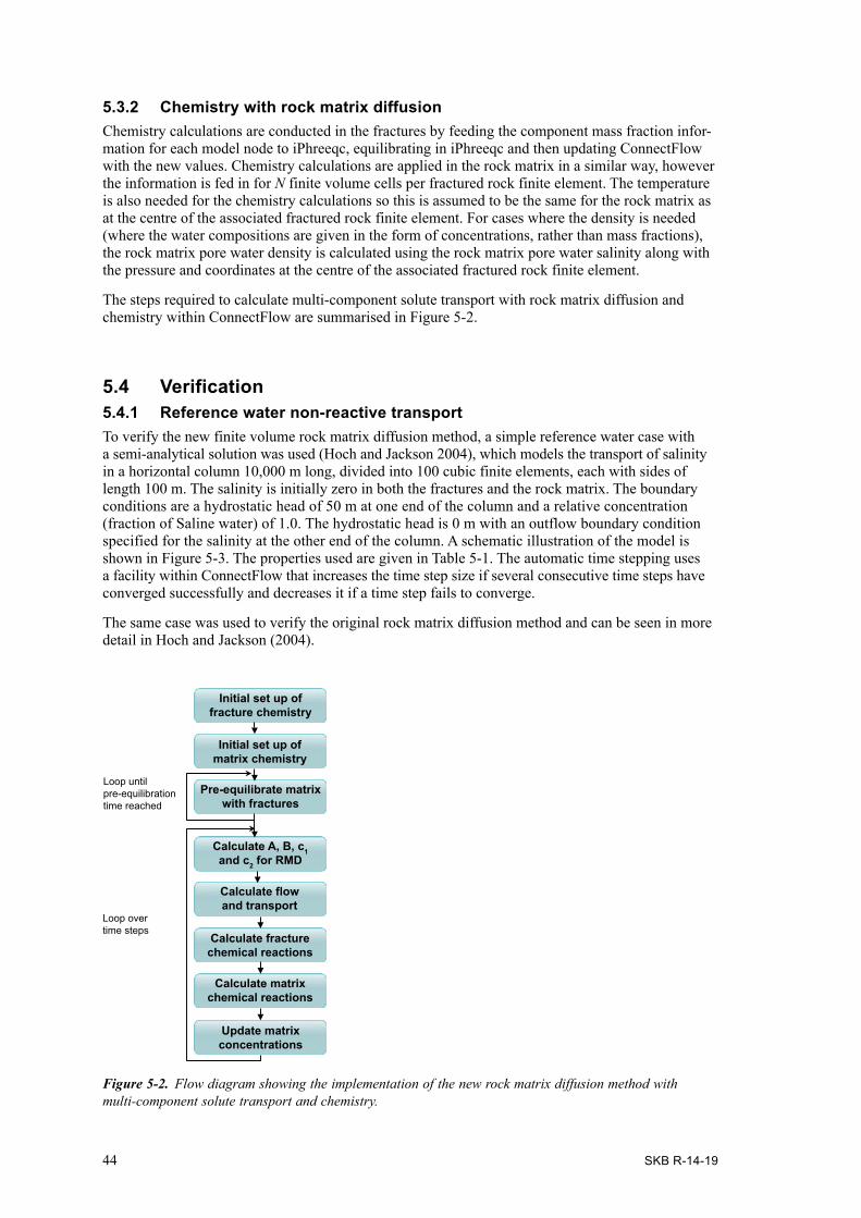
44 SKB R-14-19

5.3.2 Chemistry with rock matrix diffusionChemistry calculations are conducted in the fractures by feeding the component mass fraction infor-mation for each model node to iPhreeqc, equilibrating in iPhreeqc and then updating ConnectFlow with the new values. Chemistry calculations are applied in the rock matrix in a similar way, however the information is fed in for N finite volume cells per fractured rock finite element. The temperature is also needed for the chemistry calculations so this is assumed to be the same for the rock matrix as at the centre of the associated fractured rock finite element. For cases where the density is needed (where the water compositions are given in the form of concentrations, rather than mass fractions), the rock matrix pore water density is calculated using the rock matrix pore water salinity along with the pressure and coordinates at the centre of the associated fractured rock finite element.

The steps required to calculate multi-component solute transport with rock matrix diffusion and chemistry within ConnectFlow are summarised in Figure 5-2.

5.4 Verification5.4.1 Reference water non-reactive transportTo verify the new finite volume rock matrix diffusion method, a simple reference water case with a semi-analytical solution was used (Hoch and Jackson 2004), which models the transport of salinity in a horizontal column 10,000 m long, divided into 100 cubic finite elements, each with sides of length 100 m. The salinity is initially zero in both the fractures and the rock matrix. The boundary conditions are a hydrostatic head of 50 m at one end of the column and a relative concentration (fraction of Saline water) of 1.0. The hydrostatic head is 0 m with an outflow boundary condition specified for the salinity at the other end of the column. A schematic illustration of the model is shown in Figure 5-3. The properties used are given in Table 5-1. The automatic time stepping uses a facility within ConnectFlow that increases the time step size if several consecutive time steps have converged successfully and decreases it if a time step fails to converge.

The same case was used to verify the original rock matrix diffusion method and can be seen in more detail in Hoch and Jackson (2004).

Figure 5‑2. Flow diagram showing the implementation of the new rock matrix diffusion method with multi-component solute transport and chemistry.

Loop until pre-equilibration time reached

Loop over time steps

Initial set up of fracture chemistry

Initial set up of matrix chemistry

Pre-equilibrate matrix with fractures

Calculate A, B, c1 and c2 for RMD

Calculate flow and transport

Calculate fracture chemical reactions

Calculate matrix chemical reactions

Update matrix concentrations

SKB R-14-19 45

Table 5-1. Property values for the reference water non-reactive transport case.

Property Value


Solute diffusion coefficient 1.0∙10–9 m2/sSolute longitudinal dispersion length 100 mSolute transverse dispersion length 10 mTemperature 20°CFluid viscosity 1.0∙10–3 Pa/sFluid density 9.98∙102 kg/m3

Time step size 1.0∙107 s initially but automatically adjusted Number of time steps 501Kinematic porosity, φf 0.01Matrix capacity factor, α 0.3Intrinsic diffusion coefficient, Di 5.0∙10–11 m2/sSpecific fracture surface area, σ 2.0 m–1

Maximum matrix penetration depth, d 0.5 m

The number of finite volume cells is set to 5, 10 or 20 cells per fractured rock finite element. For each case, the finite volume cells are set to be of equal size. Results are compared with the analytical solution as shown in Figure 5-4 and Figure 5-5. Both figures show that the finite volume method agrees well with the analytical method, with the agreement improving as the number of finite volume cells is increased.

As it is possible to use non-uniform cell sizes to represent the rock matrix, the effect of this was also investigated for the verification case. The rock matrix is split into five cells in the distributions shown below in Figure 5-6. The original distribution (used in the verification case with results shown above) has all rock matrix cells of equal size. Distributions 2, 4 and 5 have the cells increasing in size away from the fracture and distribution 3 has the cells decreasing in size away from the fracture.

The results of the investigation into the effects of rock matrix cell size are shown in Figure 5-7, where the concentrations are compared against the results from the previous verification runs. This figure shows that having large cell sizes close to the fracture (distribution 3) decreases the accuracy of the solution. However, reducing the cell size close to the fracture improves accuracy, to the extent that by using five cells in distribution 5, the accuracy is the same as using 20 equal length cells. This is because the bulk of the diffusion into and out of the rock matrix occurs close to the fracture, so reducing the size of the cells closest to the fracture increases the accuracy. In cases where solutes diffuse further into the rock matrix, altering the cell sizes may not be as effective, but distributions where the cells decrease in size close to the fracture would still be expected to improve the accuracy.

The analysis in this section has provided verification for the finite volume rock matrix diffusion scheme against an analytical solution. It has also shown that increasing the number of finite volume cells used increases the accuracy, and that this effect can also be achieved by altering the distribution of cell sizes so that the smallest cells are nearest the fracture. This can improve the accuracy without impacting the performance.

Figure 5‑3. Schematic illustration of the reference water non-reactive transport RMD verification case.

FractureSALINE GLACIAL WATER

Rock matrix

Rock matrix

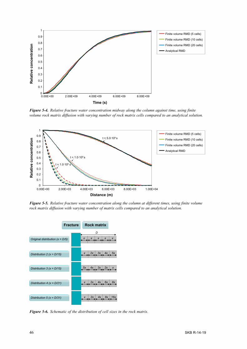
46 SKB R-14-19

Figure 5‑6. Schematic of the distribution of cell sizes in the rock matrix.

Figure 5‑4. Relative fracture water concentration midway along the column against time, using finite volume rock matrix diffusion with varying number of rock matrix cells compared to an analytical solution.

Figure 5‑5. Relative fracture water concentration along the column at different times, using finite volume rock matrix diffusion with varying number of matrix cells compared to an analytical solution.

0

0.1

0.2

0.3

0.4

0.5

0.6

0.7

0.8

0.9

1

0.00E+00 2.00E+09 4.00E+09 6.00E+09 8.00E+09

Rel

ativ

e co

ncen

trat

ion

Time (s)

Finite volume RMD (5 cells)



Analytical RMD

0

0.1

0.2

0.3

0.4

0.5

0.6

0.7

0.8

0.9

1

0.00E+00 2.00E+03 4.00E+03 6.00E+03 8.00E+03 1.00E+04

Rel

ativ

e co

ncen

trat

ion

Distance (m)

t = 1.0∙109 s

t = 1.0∙108 s

t = 5.0∙109 sFinite volume RMD (5 cells)



Analytical RMD

x 2x 3x 4x 5x

x 2x 4x 6x 8x

x 2x 4x 8x 16x

5x 4x 3x 2x x

x x x x x

D

Original distribution (x = D/5)

Distribution 2 (x = D/15)




Rock matrixFracture

x 2x 3x 4x 5x

x 2x 4x 6x 8x

x 2x 4x 8x 16x

5x 4x 3x 2x x

x x x x x

D

Original distribution (x = D/5)





Rock matrixFracture

SKB R-14-19 47

Figure 5‑7. Relative concentration along the column at time t=1.0∙108 s, using finite volume (FV) rock matrix diffusion (RMD) with varying number of matrix cells and different cell sizes compared to an analytical solution.

0

0.1

0.2

0.3

0.4

0.5

0.6

0.7

0.8

0.9

1

0.00E+00 2.00E+03 4.00E+03

Rel

ativ

e co

ncen

trat

ion

Distance (m)

FV RMD 5

FV RMD 20

FV RMD 5 (distribution 2)

Analytical RMD




FV RMD 10

5.4.2 Multi-component solute transport and equilibration with calciteThis verification case uses the model described in Section 3.3, consisting of a horizontal column filled with sea water in equilibrium with calcite, and glacial water is introduced at the upstream end. However, the Darcy flux was increased by a factor of ten to 3.17∙10–12 m/s (1.0∙10–4 m/y) and the time step size was reduced by a factor of ten to 3.157∙106 s (0.1 y) to make the flow in the fractures more advection dominated (relative to diffusion), and hence more of a contrast with the diffusion in the rock matrix. The RMD parameters used are given in Table 5-2.

The model is initially run without chemistry and the results are compared against the original RMD method. The calcium mass fraction profiles after six years from this model without chemical reac-tions are shown in Figure 5-8 for different distributions of finite volume cell sizes. The results are in reasonable agreement with the original rock matrix diffusion method, but the agreement improves as the number of finite volume cells is increased. If the rock matrix cells are sized as in distribution 2 in Figure 5-6, then an improvement in results is seen.

Table 5-2. RMD parameter values for the calcite equilibration reactive transport case.

RMD parameter Value

Kinematic porosity, φf 1.0∙10–4

Matrix capacity factor, α 3.0∙10–3

Intrinsic diffusion coefficient, Di 1.0∙10–13 m2/sSpecific fracture surface area, σ 1.0 m–1

Maximum penetration depth, d 1.0 m

To investigate the effect of rock matrix diffusion on the model including chemistry, a number of cases were run and the results were compared to cases without chemistry and without rock matrix diffusion. Figure 5-9 shows the distribution in the mass fraction of sodium along the length of the model after six years. In this case, sodium is non-reactive, so including chemistry is not expected to affect its mass fraction. Rock matrix diffusion raises the sodium mass fraction in the fractures due to diffusion out of the rock matrix.

Figure 5-10 shows the distribution in the mass fraction of calcium along the length of the model after six years. Five finite volume cells were used to discretise the rock matrix. In this case, calcium is reactive, so including chemistry is expected to have an effect on its mass fraction in solution. The effect of chemistry is to slightly decrease the calcium mass fraction in solution due to precipitation

48 SKB R-14-19

of calcite. In this case, the chemistry has a much smaller effect than rock matrix diffusion. A rock matrix diffusion case has also been run with a 2% calculation threshold applied for the chemistry (as described in Section 2.4.8). Figure 5-10 shows that this model produces nearly identical results to the equivalent model without a calculation threshold.

Figure 5‑8. Calcium mass fraction along the model column at 6 years, using finite volume (FV) rock matrix diffusion (RMD) with varying number of rock matrix cells and the original rock matrix diffusion method. Chemistry not included.

Figure 5‑9. Sodium mass fraction along the column at 6 years, using the finite volume (FV) rock matrix diffusion (RMD) method with and without chemistry. A case with a 2% chemistry calculation threshold is also included. The “No RMD, no chemistry” line is hidden below the “Chemistry, no RMD” line.

0.0E+00

1.0E-05

2.0E-05

3.0E-05

4.0E-05

5.0E-05

6.0E-05

7.0E-05

0.0 2.0 4.0 6.0 8.0 10.0

Distance (m)

Ca

(kg/

kgs)

No RMD

Original RMD

FV RMD (5 cells)

FV RMD (5 cells, dist 2)

FV RMD (10 cells)

FV RMD (10 cells, dist 2)

FV RMD (20 cells)

Sea

Glacial

0.0E+00

5.0E-04

1.0E-03

1.5E-03

2.0E-03

2.5E-03

3.0E-03

0.0 2.0 4.0 6.0 8.0 10.0

Distance (m)

Na

(kg/

kgs)

No RMD, no chemistry

Chemistry, no RMD

No chemistry, FV RMD 5

Chemistry, FV RMD 5

Chemistry, FV RMD 5 – 2% threshold

Sea

Glacial

SKB R-14-19 49

Figure 5‑10. Calcium mass fraction along the model column at 6 years, using the finite volume rock matrix diffusion method, with and without chemistry.

0.0E+00

1.0E-05

2.0E-05

3.0E-05

4.0E-05

5.0E-05

6.0E-05

7.0E-05

0.0 2.0 4.0 6.0 8.0 10.0

Distance (m)

Ca

(kg/

kgs)

No RMD, no chemistry

Chemistry, no RMD

No chemistry, FV RMD 5

Chemistry, FV RMD 5

Chemistry, FV RMD 5 – 2% threshold

Sea

Glacial

SKB R-14-19 51

6 Performance and parallelisation

6.1 Chemistry and equation assemblyIt is essential that reactive transport calculations can be carried out on a reasonable time scale. Therefore, it is important to ensure that the most time consuming parts of the calculations are carried out as efficiently as possible. Usually it is the calculation of the chemical reactions that are the slowest parts of any reactive transport simulation. However, these calculations are carried out independently for each reaction cell and so lend themselves well to parallelisation. Therefore, the chemistry calculations within ConnectFlow have been parallelised by sub-dividing the calculations amongst the available processors using the message passing interface (MPI) method. This has enabled a significant speed up of the chemistry calculations, which scales well with the number of processors used. Use of the parallel solvers in ConnectFlow, such as the Hypre AMG solver, for the flow and transport calculations can also provide performance improvements when run on multiple processors.

After chemistry, the assembly of the transport equations is responsible for the majority of the run-time. Equation assembly is the process by which the matrix representing the linear system of equations to solve is constructed. In CPM models this includes calculating contributions from each finite element. Analysis shows that around 80-90% of this process is carried out independently for each finite element. Therefore, the equation assembly lends itself well to parallelisation, since the calculation of the contributions from the finite elements can be distributed amongst the available processors.

Figure 6-5 shows the total amount of time taken for each stage of a ConnectFlow multi-component solute transport calculation over ten time steps for the Forsmark palaeo-climate calculation described in Section 7.1.5. This case has about 1.2 million finite elements, four mineral phases and eighteen components. Figure 6-6 shows the same information as a percentage of the total calculation time. It can be seen that for a single processor, the run-time is dominated by the chemistry calculations, with the assembly of the transport equations also significant. However, since the chemistry paral-lelises well, the proportion of the time spent carrying out chemical calculations decreases rapidly with the number of processors. Figure 6-8 shows how this performance scales relative to that for a single processor. The chemistry calculations show good scaling up to 12 processor cores (on a 2 CPU computer with 8 cores per CPU), which was the largest number of processors tried. There is also reasonable scaling of performance with the number of processors for the flow and transport equation assembly. The groundwater flow calculations also scale reasonably well using the Hypre AMG solver. The transport calculations scale less well, probably because the calculation for each component is relatively quick so the performance improvements from parallelisation are offset by the overheads of running in parallel, such as distributing data to processors.

As described in Section 2.4.8, calculation thresholds can also be used to improve performance by only requiring chemistry calculations to be carried out in parts of the model where the composition of the water is changing significantly. Figure 6-4 shows how the performance of the chemistry calculations is affected by using a 2% calculation threshold. It can be seen that during the early part of the calculations use of the calculation threshold gives nearly a factor two increase in performance. However, at around 6000 BC, the system begins to evolve more rapidly as Littorina water is intro-duced and begins to migrate through the model, and the benefit of using the calculation threshold is reduced. As the system stabilises, use of the calculation threshold again provides a benefit until the system begins to evolve again upon the introduction of Meteoric water at around 1000 AD. The effect on performance of using a calculation threshold will be model specific and will depend on the proportion of the model where the solute composition is changing very little.

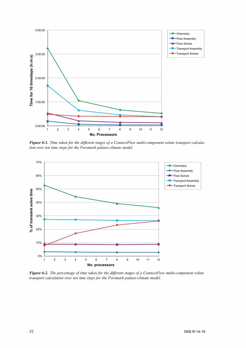
52 SKB R-14-19

Figure 6‑1. Time taken for the different stages of a ConnectFlow multi-component solute transport calcula-tion over ten time steps for the Forsmark palaeo-climate model.

Figure 6‑2. The percentage of time taken for the different stages of a ConnectFlow multi-component solute transport calculation over ten time steps for the Forsmark palaeo-climate model.

0:00:00

1:00:00

2:00:00

3:00:00

4:00:00

1 2 3 4 5 6 7 8 9 10 11 12

No. Processors

Tim

e fo

r 10

times

teps

(h:m

:s)

Chemistry

Flow Assembly

Flow Solves

Transport Assembly

Transport Solves

Chemistry

Flow Assembly

Flow Solves

Transport Assembly

Transport Solves

0%

10%

20%

30%

40%

50%

60%

70%

1 2 3 4 5 6 7 8 9 10 11 12

No. processors

% o

f tra

nsie

nt s

olve

tim

e

SKB R-14-19 53

Figure 6‑3. The performance relative to one processor for the different stages of a ConnectFlow multi-component solute transport calculation over ten time steps for the Forsmark palaeo-climate model.

Chemistry

Flow Assembly

Flow Solves

Transport Assembly

Transport Solves

0.0

1.0

2.0

3.0

4.0

5.0

6.0

7.0

8.0

1 2 3 4 5 6 7 8 9 10 11 12

No. processors

Perf

orm

ance

rela

tive

to 1

pro

cess

or

00:02:00

00:03:00

00:04:00

00:05:00

00:06:00

00:07:00

-8000 -7000 -6000 -5000 -4000 -3000 -2000 -1000 0 1000 2000

Year AD (1 timestep = 20 years)

Che

mis

try

time

per t

imes

tep

(h:m

:s)

Chemistry (0% threshold, 4 CPU)

Chemistry (2% threshold, 4 CPU)

Introduction of Littorina

Introduction of Meteroic

Figure 6‑4. Time taken for the chemistry calculations for each timestep during a ConnectFlow multi-component solute transport calculation for the Forsmark palaeo-climate model. The performance with a 2% calculation threshold is compared to that without a calculation threshold.

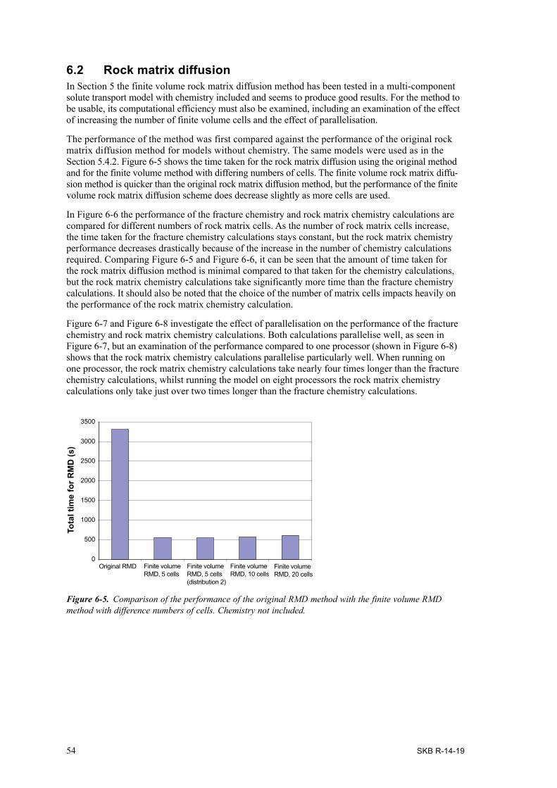
54 SKB R-14-19

6.2 Rock matrix diffusionIn Section 5 the finite volume rock matrix diffusion method has been tested in a multi-component solute transport model with chemistry included and seems to produce good results. For the method to be usable, its computational efficiency must also be examined, including an examination of the effect of increasing the number of finite volume cells and the effect of parallelisation.

The performance of the method was first compared against the performance of the original rock matrix diffusion method for models without chemistry. The same models were used as in the Section 5.4.2. Figure 6-5 shows the time taken for the rock matrix diffusion using the original method and for the finite volume method with differing numbers of cells. The finite volume rock matrix diffu-sion method is quicker than the original rock matrix diffusion method, but the performance of the finite volume rock matrix diffusion scheme does decrease slightly as more cells are used.

In Figure 6-6 the performance of the fracture chemistry and rock matrix chemistry calculations are compared for different numbers of rock matrix cells. As the number of rock matrix cells increase, the time taken for the fracture chemistry calculations stays constant, but the rock matrix chemistry performance decreases drastically because of the increase in the number of chemistry calculations required. Comparing Figure 6-5 and Figure 6-6, it can be seen that the amount of time taken for the rock matrix diffusion method is minimal compared to that taken for the chemistry calculations, but the rock matrix chemistry calculations take significantly more time than the fracture chemistry calculations. It should also be noted that the choice of the number of matrix cells impacts heavily on the performance of the rock matrix chemistry calculation.

Figure 6-7 and Figure 6-8 investigate the effect of parallelisation on the performance of the fracture chemistry and rock matrix chemistry calculations. Both calculations parallelise well, as seen in Figure 6-7, but an examination of the performance compared to one processor (shown in Figure 6-8) shows that the rock matrix chemistry calculations parallelise particularly well. When running on one processor, the rock matrix chemistry calculations take nearly four times longer than the fracture chemistry calculations, whilst running the model on eight processors the rock matrix chemistry calculations only take just over two times longer than the fracture chemistry calculations.

Figure 6‑5. Comparison of the performance of the original RMD method with the finite volume RMD method with difference numbers of cells. Chemistry not included.

0

500

1000

1500

2000

2500

3000

3500

Original RMD

Tota

l tim

e fo

r RM

D (s

)

Finite volume RMD, 5 cells (distribution 2)

Finite volume RMD, 5 cells



SKB R-14-19 55

Figure 6‑6. Comparison of the performance of the chemistry calculation for the finite volume RMD scheme with difference numbers of cells.

0

10000

20000

30000

40000

50000

60000

70000

80000

90000

5 cells 5 cells(distribution 2)

5 cells (2%threshhold)

10 cells 20 cells

Tota

l tim

e (s

)

Rock matrix chemistry time

Fracture chemistry time

Figure 6‑7. Performance of the fracture chemistry and rock matrix chemistry calculations for different numbers of processors (5 equally spaced rock matrix cells used).

0

2000

4000

6000

8000

10000

12000

14000

16000

18000

20000

0 1 2 3 4 5 6 7 8 9

No. processors

Tota

l tim

e (s

)

Fracture chemistry time

Rock matrix chemistry time

Figure 6‑8. Performance relative to one processor of the fracture chemistry and rock matrix chemistry calculations for different numbers of processors (5 equally spaced rock matrix cells used).

0

1

2

3

4

5

6

7

8

9

0 1 2 3 4 5 6 7 8 9

No. processors

Perf

orm

ance

rela

tive

to 1

pro

cess

or Fracture chemisty performance

Rock matrix chemistry performance

SKB R-14-19 57

7 Applications

This section provides illustrations of the types of situation that the new ConnectFlow reactive transport functionality can be applied to. In particular, they demonstrate that the method can be applied to large-scale models that are relevant to the safety assessments of Forsmark and Olkiluoto and produce results that are not inconsistent with site data and previous studies. As these calculations are illustrative, the results are not intended to replace or update hydrogeochemical modelling results already obtained for these sites.

7.1 Forsmark palaeo-climate calculations7.1.1 BackgroundThe license application submitted by SKB for a spent nuclear fuel repository at Forsmark is supported by the SR-Site safety assessment to demonstrate the long-term safety of the proposed repository (SKB 2011). Temperate climate period modelling was used to calculate the regional evolution of groundwater composition for the time span 8000 BC to 12,000 AD as part of SR-Site (Joyce et al. 2010). This corresponds to the current Holocene period that started at the end of the Weichselian glaciation, but is also taken to represent future inter-glacial periods. The interval from 8000 BC to around 1000 AD corresponds to a time when the Forsmark site was submerged. The subsequent interval up to 12,000 AD corresponds to a period when the site is above sea level and the shoreline is retreating due to post-glacial land rise. The reference glacial cycle (SKB 2010a) predicts that the Holocene period will continue to 9000 AD, corresponding to the first occurrence of permafrost. The reference glacial cycle corresponds to the SR-Site base case.

Calculations of hydrogeochemistry were carried out to provide input to the determination of the relevant safety functions for SR-Site (Salas et al. 2010). These calculations were based on reference water fractions exported from the temperate period regional-scale models. The reference water fractions implied a groundwater composition at the locations of interest (typically vertical and horizontal slices through the repository volume), which enabled chemical equilibration calculations with mineral phases to be carried out at these locations using PHREEQC.

The approach reported here is similar, but uses the new multi-component reactive transport facility of ConnectFlow to carry out the equilibration reactions at all points in the model at each time step. Hence there is far more continuity, both in space and time, in the chemistry calculations compared to the post-processing approach used for SR-Site.

7.1.2 Hydrogeological Conceptual ModelThe Forsmark site consists of fractured crystalline rock overlain with Quaternary deposits. Based on the characteristics of the geology, the rock was sub-divided into rock domains (SKB 2008), as shown in Figure 7-1. The repository itself is located in a so-called tectonic lens in which the bedrock is less affected by ductile deformation within surrounding belts of high ductile strain. The upper 200 m of the bedrock is characterised by an increased intensity of sub-horizontal to gently dipping fractures and sheet-joints forming a shallow bedrock aquifer. Below this is sparsely fractured bedrock of low permeability. The intensity of fractures generally decreases with increasing depth.

A conceptual model of the site hydrogeology was developed during the site-descriptive modelling (SDM), culminating in SDM-Site (SKB 2008), serving as a basis for the SR-Site safety assessment (SKB 2011). The conceptual model describes three hydraulic domains (illustrated in Figure 7-2):

• HCD (Hydraulic Conductor Domain) representing deformation zones. The deformation zones forming the HCD are defined as structures where there is a concentration of brittle, ductile or combined brittle and ductile deformation. They are envisaged as being composed of swarms of smaller fractures.

58 SKB R-14-19

• HRD (Hydraulic Rock mass Domain) representing the less fractured bedrock in between the deformation zones. The fractured bedrock between the deformation zones was divided into a number of fracture domains, characterised by fracture properties and location. These fracture domains were denoted FFM01 to FFM06 and are shown schematically in Figure 7-3 and Figure 7-4. Fracture domain FFM06 has a similar structural context to FFM01 and so these two fracture domains were merged.

• HSD (Hydraulic Soil Domain) representing the regolith (Quaternary deposits). The conceptual model of the HSD consists of nine layers (L1-L3 and Z1-Z6) of varying extents and thicknesses as shown in Figure 7-5.

Figure 7‑1. Illustrations of the rock domains at the surface of the local model areas for Forsmark. (SKB 2008).

Figure 7‑2. Schematic diagram showing the division of the crystalline bedrock and the regolith (Quaternary deposits) into three hydraulic domains, HCD, HRD and HSD. (Rhén et al. 2003).

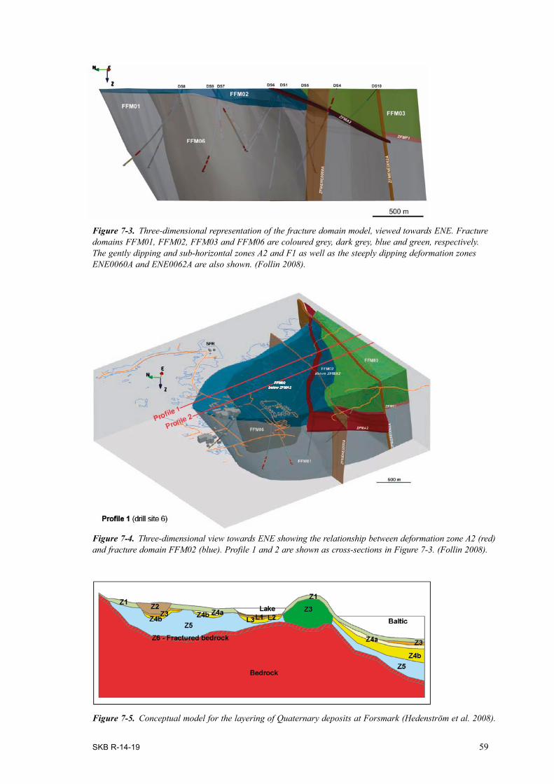
SKB R-14-19 59

Figure 7‑3. Three-dimensional representation of the fracture domain model, viewed towards ENE. Fracture domains FFM01, FFM02, FFM03 and FFM06 are coloured grey, dark grey, blue and green, respectively. The gently dipping and sub-horizontal zones A2 and F1 as well as the steeply dipping deformation zones ENE0060A and ENE0062A are also shown. (Follin 2008).

Figure 7‑4. Three-dimensional view towards ENE showing the relationship between deformation zone A2 (red) and fracture domain FFM02 (blue). Profile 1 and 2 are shown as cross-sections in Figure 7-3. (Follin 2008).

Figure 7‑5. Conceptual model for the layering of Quaternary deposits at Forsmark (Hedenström et al. 2008).

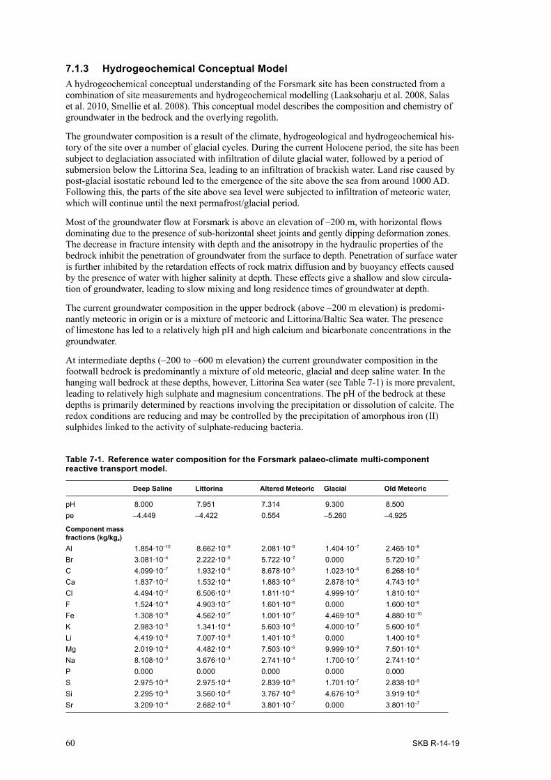
60 SKB R-14-19

7.1.3 Hydrogeochemical Conceptual ModelA hydrogeochemical conceptual understanding of the Forsmark site has been constructed from a combination of site measurements and hydrogeochemical modelling (Laaksoharju et al. 2008, Salas et al. 2010, Smellie et al. 2008). This conceptual model describes the composition and chemistry of groundwater in the bedrock and the overlying regolith.

The groundwater composition is a result of the climate, hydrogeological and hydrogeochemical his-tory of the site over a number of glacial cycles. During the current Holocene period, the site has been subject to deglaciation associated with infiltration of dilute glacial water, followed by a period of submersion below the Littorina Sea, leading to an infiltration of brackish water. Land rise caused by post-glacial isostatic rebound led to the emergence of the site above the sea from around 1000 AD. Following this, the parts of the site above sea level were subjected to infiltration of meteoric water, which will continue until the next permafrost/glacial period.

Most of the groundwater flow at Forsmark is above an elevation of –200 m, with horizontal flows dominating due to the presence of sub-horizontal sheet joints and gently dipping deformation zones. The decrease in fracture intensity with depth and the anisotropy in the hydraulic properties of the bedrock inhibit the penetration of groundwater from the surface to depth. Penetration of surface water is further inhibited by the retardation effects of rock matrix diffusion and by buoyancy effects caused by the presence of water with higher salinity at depth. These effects give a shallow and slow circula-tion of groundwater, leading to slow mixing and long residence times of groundwater at depth.

The current groundwater composition in the upper bedrock (above –200 m elevation) is predomi-nantly meteoric in origin or is a mixture of meteoric and Littorina/Baltic Sea water. The presence of limestone has led to a relatively high pH and high calcium and bicarbonate concentrations in the groundwater.

At intermediate depths (–200 to –600 m elevation) the current groundwater composition in the footwall bedrock is predominantly a mixture of old meteoric, glacial and deep saline water. In the hanging wall bedrock at these depths, however, Littorina Sea water (see Table 7-1) is more prevalent, leading to relatively high sulphate and magnesium concentrations. The pH of the bedrock at these depths is primarily determined by reactions involving the precipitation or dissolution of calcite. The redox conditions are reducing and may be controlled by the precipitation of amorphous iron (II) sulphides linked to the activity of sulphate-reducing bacteria.

Table 7-1. Reference water composition for the Forsmark palaeo-climate multi-component reactive transport model.

Deep Saline Littorina Altered Meteoric Glacial Old Meteoric

pH 8.000 7.951 7.314 9.300 8.500pe –4.449 –4.422 0.554 –5.260 –4.925

Component mass fractions (kg/kgs)Al 1.854∙10–10 8.662∙10–9 2.081∙10–9 1.404∙10–7 2.465∙10–8

Br 3.081∙10–4 2.222∙10–5 5.722∙10–7 0.000 5.720∙10–7

C 4.099∙10–7 1.932∙10–5 8.678∙10–5 1.023∙10–6 6.268∙10–6

Ca 1.837∙10–2 1.532∙10–4 1.883∙10–5 2.878∙10–6 4.743∙10–5

Cl 4.494∙10–2 6.506∙10–3 1.811∙10–4 4.999∙10–7 1.810∙10–4

F 1.524∙10–6 4.903∙10–7 1.601∙10–6 0.000 1.600∙10–6

Fe 1.308∙10–8 4.562∙10–7 1.001∙10–7 4.469∙10–8 4.880∙10–10

K 2.983∙10–5 1.341∙10–4 5.603∙10–6 4.000∙10–7 5.600∙10–6

Li 4.419∙10–6 7.007∙10–8 1.401∙10–8 0.000 1.400∙10–8

Mg 2.019∙10–6 4.482∙10–4 7.503∙10–6 9.999∙10–8 7.501∙10–6

Na 8.108∙10–3 3.676∙10–3 2.741∙10–4 1.700∙10–7 2.741∙10–4

P 0.000 0.000 0.000 0.000 0.000S 2.975∙10–6 2.975∙10–4 2.839∙10–5 1.701∙10–7 2.838∙10–5

Si 2.295∙10–6 3.560∙10–6 3.767∙10–6 4.676∙10–6 3.919∙10–6

Sr 3.209∙10–4 2.682∙10–6 3.801∙10–7 0.000 3.801∙10–7

SKB R-14-19 61

Figure 7‑6. Local area model for the Forsmark palaeo-climate reactive transport calculations, viewed from above and coloured by the vertical component of hydraulic conductivity. The hydraulic soil domain has been removed in the figure. The black line indicates the boundary of the SR-Site regional-scale model.

At greater depths (below –600 m elevation) the salinity increases as deep saline water predominates. The presence of crystalline oxides, such as haematite, indicates reducing conditions and long residence times for the groundwater.

The geochemical conceptual model assumes that the groundwater composition is determined primarily by a mixing of waters of different origins, driven by groundwater flow and transport processes. However, chemical reactions are required to gain a full understanding of the groundwater composition, pH and redox conditions. These reactions are with fracture-filling minerals and with rock forming minerals. The selected minerals for SR-Site are those present at Forsmark as fracture fillings with fast kinetics compared to the time intervals considered (calcite and iron (III) oxyhydroxides) or those that appear to be in equilibrium with current groundwaters (quartz, hydroxyapatite and amorphous iron (II) monosulphides). Iron (III) oxyhydroxide and amorphous iron (II) monosulphides are two alternatives, where the former represents a system which is not affected by sulphate-reducing bacteria and the latter a situation in which there is significant activity of sulphate-reducing bacteria (Salas et al. 2010). The selected minerals are assumed to be in equilibrium with the groundwater at all locations and times. In addition, it is assumed that these minerals are present in sufficient quantity such that they will not be depleted.

7.1.4 Numerical ModelThe model considered here consists of the local sub-volume of the SR-Site regional-scale temperate period model, as shown in Figure 7-6. This is approximately 4.0 km by 5.0 km and 1.2 km deep, sub-divided horizontally into 100 m finite elements, with 20 m refinement in the 3 km × 3 km area containing the repository volume, as shown in Figure 7-7. Internal boundary conditions ensure continuity of pressure and flow where there are discontinuities in the grid at the boundaries of the local area. The top surface of the model is mapped to the topography. There are around 1.2 million finite elements in total.

62 SKB R-14-19

Figure 7‑7. Local area model for the Forsmark palaeo-climate reactive transport calculations, viewed in 3D perspective and coloured by the vertical component of hydraulic conductivity. The hydraulic soil domain has been removed in the figure. The edges of the finite elements are shown in black.

The bedrock is represented by an equivalent continuous porous medium (ECPM). The hydraulic properties are obtained by upscaling a regional-scale discrete fracture network (DFN) model of the HRD, combined with the application of deformation zone and sheet joint properties using the implicit fracture zone method (IFZ) (Hartley and Joyce 2013). The Hydraulic Soil Domain (HSD) is represented by four 1 m deep layers. The vertical and horizontal components of the HSD hydraulic conductivity are different, i.e. the hydraulic conductivity is anisotropic. The horizontal component of the conductivity tensor is based on the arithmetic mean of the hydraulic properties of the original stratigraphy, whereas the vertical component is based on its harmonic mean.

The reference water compositions used in the specification of the initial conditions and boundary conditions are shown in Table 7-1, equivalent to Table 4-2 in Salas et al. (2010). These are converted to component mass fractions by ConnectFlow, which are then used in the transport calculations. The initial condition at 8000 BC is the same as for SR-Site (Joyce et al. 2010), i.e. Deep Saline water in the lower part of the model, being replaced by a mixture of Old Meteoric and Glacial waters higher in the model, with the proportions of the waters a function of elevation.

The boundary conditions for the sides of the model specify zero flux of water and zero flux of solute. The boundary condition on the bottom of the model specifies zero flux of water and the mass fractions of the solutes are held constant at their initial values. The top surface boundary condition leads to recharge or discharge of water depending on the calculated head relative to the ground surface elevation (taking land rise, the depth of the sea and the salinity of the sea into account). The composition of infiltrating water through the top boundary varies over time, consisting of Glacial water at early times, followed by Littorina Sea water for parts of the surface below the sea and then meteoric water for land areas above sea level.

SKB R-14-19 63

Groundwater flow and multi-component solute transport calculations are carried out over the time period 8000 BC to 2000 AD in 20 year time steps. The calculations are carried out with and without chemical reactions. A total of 18 chemical species are transported. The effects of groundwater composition and temperature on groundwater density and viscosity are included, which affect the direction and magnitude of groundwater flow. A temperature of 6ºC is specified at the ground surface which increases at 0.01ºC/m with depth.

The chemical reactions included are the equilibration with calcite, quartz, hydroxyapatite and amorphous iron(II) sulphide (FeS(ppt)). This corresponds to the base case in Salas et al. (2010) for the situation with significant activity of sulphate-reducing bacteria and uses the same thermody-namic database. Initially, the reference waters are equilibrated with these mineral phases and charge balanced by adjusting the mass fraction of sodium or chloride ions as necessary. The equilibration reactions with these four minerals are then repeated for each time step using the updated solute compositions from the transport calculations. Each mineral has an initial quantity of 10 mol/kgw (the default for PHREEQC and ConnectFlow) throughout the model, which essentially means that it will not be depleted. The temperature at each location where chemical reactions are carried out is taken into account in the calculations.

7.1.5 Effective porosity modelThis case is a baseline model for multi-component reactive transport, without diffusion and chemical reactions in the rock matrix. It is equivalent to having a very high rate of diffusivity into the rock matrix. To mimic the solute retardation effects of the rock matrix, an effective porosity is used for the fractured rock based on both the fracture porosity and the rock matrix porosity. This represents the porosity accessible to transported solutes and is defined as:

mmfe dP φφφ 322+=

(7-1)

where ϕe is the effective porosity, ϕf is the fracture porosity, ϕm is the matrix porosity, P32 is the fracture surface area per unit volume and dm is the penetration depth into the matrix. For this case 2P32dm is equal to one and, since the matrix porosity is much higher than the fracture porosity, ϕe ≈ ϕm.

Figure 7-8 shows the distribution of chloride concentration with depth for boreholes KFM01, KFM02 and KFM10, located within the footwall volume of the repository candidate area. The results for simulations with and without chemistry calculations are very similar, as expected because chloride is a non-reactive component. The corresponding plot for calcium concentration in Figure 7-9 also shows little difference between the cases with and without chemistry calcula-tions, even though calcium participates in the dissolution and precipitation of calcite. In Salas et al. (2010) it is noted that, due to the high calcium concentrations in saline waters, the behaviour of calcium is almost conservative and the calcium concentrations observed can be reproduced from the mixing of reference waters alone. The plot for sulphate in Figure 7-10 does show a difference between the simulations with and without chemistry, but the differences are minor.

Figure 7-11 shows the distribution of calcium mass fraction on slices taken through the repository volume, with and without chemical reactions included. The two images are very similar although there seems to be more calcium present in solution near the top of the model when chemical reac-tions are calculated due to the dissolution of calcite by dilute infiltrating water. The mass fraction around the repository is of the order 1.0∙10–3 kg/kgs, i.e. about 2.5∙10–2 mol/L, which is consistent with the range of values reported in Salas et al. (2010).

Figure 7-12 shows the distribution of total sulphur mass fraction on slices through the repository volume. This distribution is similar to the one shown in Salas et al. (2010) where the total sulphur concentration is particularly low around the repository (approximately 1.0∙10–4 mol/L, i.e. about 3.2∙10–6 kg/kgs). There is little difference in the sulphur mass fractions in Figure 7-12 between the cases with and without chemical reactions.

64 SKB R-14-19

Figure 7‑9. Calcium concentration at 2000 AD against elevation for boreholes KFM01, KFM02 and KFM10 from an effective porosity multi-component solute transport model for Forsmark, with and without chemical reactions. Dots show measured site data. Vertical dashed lines show reference water values.

Ca, 2000AD, Foot wall

-1000

-900

-800

-700

-600

-500

-400

-300

-200

-100

00 2000 4000 6000 8000 10000 12000 14000 16000 18000 20000

Ca (mg/L)

Elev

atio

n (m

)

KFM01A (No chemistry)

Ca mg/L KFM01A

KFM01B (No chemistry)

KFM01C (No chemistry)

KFM01D (No chemistry)

Ca mg/L KFM01D


Ca mg/L Glacial

Ca mg/L Old meteoric

Ca mg/L Meteoric

Ca mg/L Deep saline

Ca mg/L Littorina

KFM01A (chemistry)

KFM01B (chemistry)

KFM01C (chemistry)

KFM01D (chemistry)

KFM02A (chemistry)

Figure 7‑8. Chloride concentration at 2000 AD against elevation for boreholes KFM01, KFM02 and KFM10 from an effective porosity multi-component solute transport model for Forsmark, with and without chemical reactions. Dots show measured site data. Vertical dashed lines show reference water values.

-1000

-900

-800

-700

-600

-500

-400

-300

-200

-100

00 5000 10000 15000 20000 25000

Elev

atio

n (m

)Cl (mg/L) Cl, 2000AD, Foot wall


Cl mg/L KFM01A




Cl mg/L KFM01D


Cl mg/L Glacial

Cl mg/L Old meteoric

Cl mg/L Meteoric

Cl mg/L Deep saline

Cl mg/L Littorina

KFM01A (chemistry)

KFM01B (chemistry)

KFM01C (chemistry)

KFM01D (chemistry)

KFM02A (chemistry)

SKB R-14-19 65

Figure 7‑10. Sulphate concentration at 2000 AD against elevation for boreholes KFM01, KFM02 and KFM10 from an effective porosity multi-component solute transport model for Forsmark, with and without chemical reactions. Dots show measured site data. Vertical dashed lines show reference water values.

SO4, 2000AD, Foot wall

-900

-1000

-800

-700

-600

-500

-400

-300

-200

-100

00 200 400 600 800 1000 1200 1400 1600

SO4 (mg/L)


SO4 mg/L KFM01A




SO4 mg/L KFM01D


SO4 mg/L Glacial

SO4 mg/L Old meteoric

SO4 mg/L Meteoric

SO4 mg/L Deep saline

SO4 mg/L Littorina

KFM01A (chemistry)

KFM01B (chemistry)

KFM01C (chemistry)

KFM01D (chemistry)

KFM02A (chemistry)

Elev

atio

n (m

)

The slices of total iron mass fraction distributions in Figure 7-13 show more of a difference between simulations with and without chemical reactions. This sensitivity may be due to the relatively low iron mass fractions in solution compared to the other ions and a dependence on the redox conditions present. The total iron mass fractions of around 1.0∙10-8 kg/kgs (approximately 2.0∙10–7 mol/L) around the repository are about an order of magnitude lower than the values calculated in Salas et al. (2010). The difference may be because this is an effective porosity model and so the details of the transport will be different and the iron mass fractions are quite sensitive to the conditions.

Figure 7-14 shows the distribution of pH values on two slices through the model for the reactive transport palaeo-climate case at 2000 AD. There is not a corresponding plot for the case without chemical reactions as pH is not calculated in that case. The calculated pH values range from about 8.0 to 9.0 at repository depth, compared to about 7.5 to 8.5 in Salas et al. (2010). The measured values from borehole samples range from 7.0 to 8.5 over all depths and are about 7.5 at repository depth.

66 SKB R-14-19

Figure 7‑11. Vertical and horizontal slices, coloured by calcium mass fraction, taken through the repository volume of the Forsmark local area equivalent porosity palaeo-climate model at 2000 AD with chemical reactions (bottom) and without chemical reactions (top). The horizontal slice is at repository depth (–470 m). The vertical slice is taken through the centre of the repository volume and extends northeast to southwest. The locations of the repository structures are shown in black for illustration, although they are not present in the model.

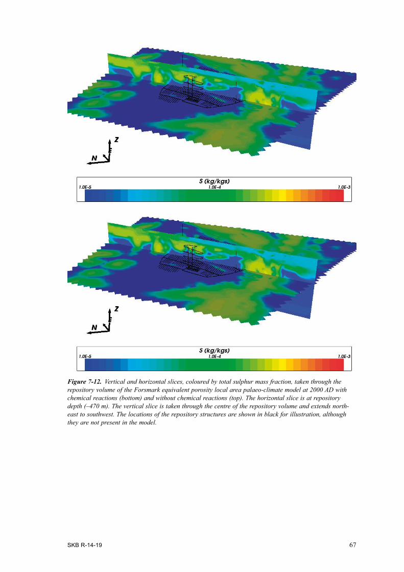
SKB R-14-19 67

Figure 7‑12. Vertical and horizontal slices, coloured by total sulphur mass fraction, taken through the repository volume of the Forsmark equivalent porosity local area palaeo-climate model at 2000 AD with chemical reactions (bottom) and without chemical reactions (top). The horizontal slice is at repository depth (–470 m). The vertical slice is taken through the centre of the repository volume and extends north-east to southwest. The locations of the repository structures are shown in black for illustration, although they are not present in the model.

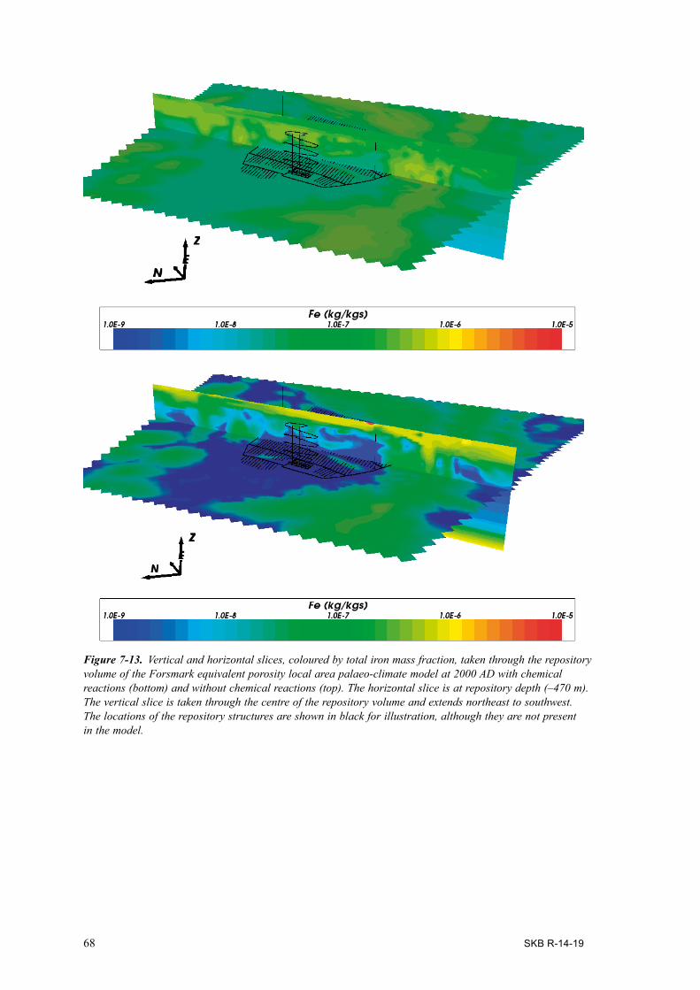
68 SKB R-14-19

Figure 7‑13. Vertical and horizontal slices, coloured by total iron mass fraction, taken through the repository volume of the Forsmark equivalent porosity local area palaeo-climate model at 2000 AD with chemical reactions (bottom) and without chemical reactions (top). The horizontal slice is at repository depth (–470 m). The vertical slice is taken through the centre of the repository volume and extends northeast to southwest. The locations of the repository structures are shown in black for illustration, although they are not present in the model.

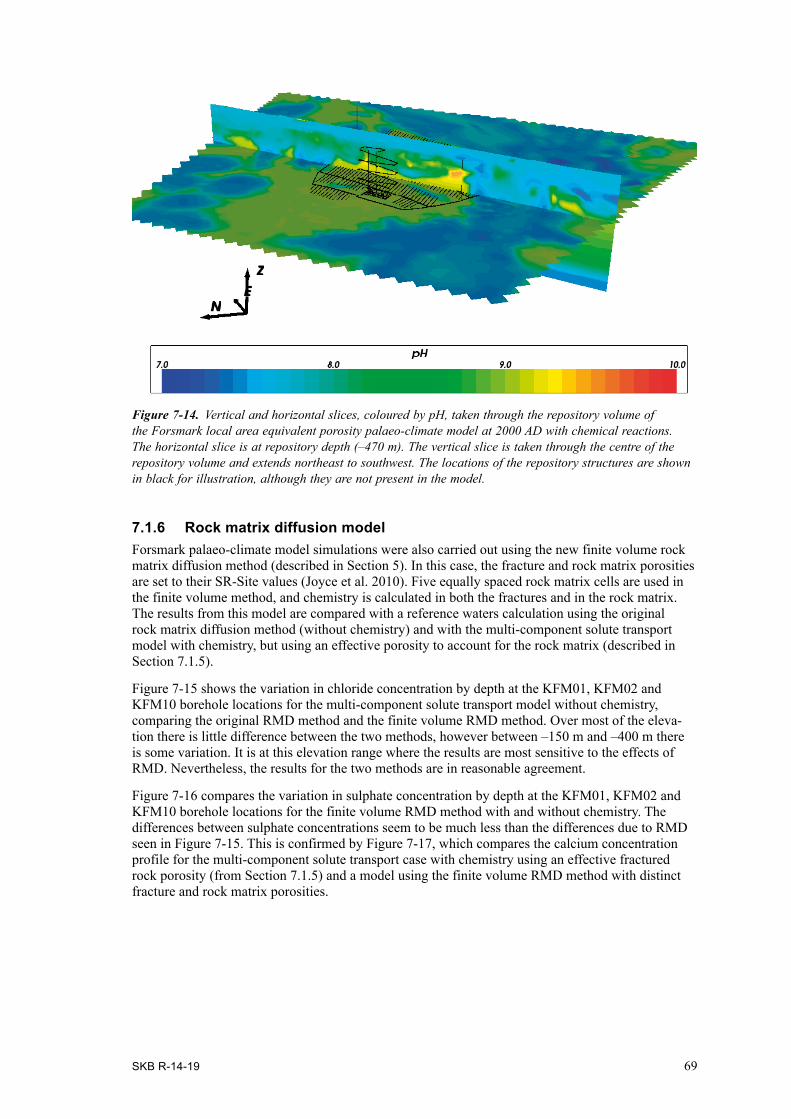
SKB R-14-19 69

Figure 7‑14. Vertical and horizontal slices, coloured by pH, taken through the repository volume of the Forsmark local area equivalent porosity palaeo-climate model at 2000 AD with chemical reactions. The horizontal slice is at repository depth (–470 m). The vertical slice is taken through the centre of the repository volume and extends northeast to southwest. The locations of the repository structures are shown in black for illustration, although they are not present in the model.

7.1.6 Rock matrix diffusion modelForsmark palaeo-climate model simulations were also carried out using the new finite volume rock matrix diffusion method (described in Section 5). In this case, the fracture and rock matrix porosities are set to their SR-Site values (Joyce et al. 2010). Five equally spaced rock matrix cells are used in the finite volume method, and chemistry is calculated in both the fractures and in the rock matrix. The results from this model are compared with a reference waters calculation using the original rock matrix diffusion method (without chemistry) and with the multi-component solute transport model with chemistry, but using an effective porosity to account for the rock matrix (described in Section 7.1.5).

Figure 7-15 shows the variation in chloride concentration by depth at the KFM01, KFM02 and KFM10 borehole locations for the multi-component solute transport model without chemistry, comparing the original RMD method and the finite volume RMD method. Over most of the eleva-tion there is little difference between the two methods, however between –150 m and –400 m there is some variation. It is at this elevation range where the results are most sensitive to the effects of RMD. Nevertheless, the results for the two methods are in reasonable agreement.

Figure 7-16 compares the variation in sulphate concentration by depth at the KFM01, KFM02 and KFM10 borehole locations for the finite volume RMD method with and without chemistry. The differences between sulphate concentrations seem to be much less than the differences due to RMD seen in Figure 7-15. This is confirmed by Figure 7-17, which compares the calcium concentration profile for the multi-component solute transport case with chemistry using an effective fractured rock porosity (from Section 7.1.5) and a model using the finite volume RMD method with distinct fracture and rock matrix porosities.

70 SKB R-14-19

Figure 7‑15. Chloride concentration at 2000 AD against elevation for boreholes KFM01, KFM02 and KFM10 from a multi-component solute transport model for Forsmark using the original RMD method and the finite volume RMD method without chemistry. Dots show measured site data. Vertical dashed lines show reference water values.

Figure 7‑16. Sulphate concentration at 2000 AD against elevation for boreholes KFM01, KFM02 and KFM10 from a multi-component solute transport model for Forsmark using the finite volume RMD method with and without chemistry. Dots show measured site data. Vertical dashed lines show reference water values.

SO4, 2000AD, Foot wall SO4 (mg/L)

Elev

atio

n (m

)

KFM01A (FV RMD no chemistry)

SO4 mg/L KFM01A

KFM01B (FV RMD no chemistry)

KFM01C (FV RMD no chemistry)

KFM01D (FV RMD no chemistry)

SO4 mg/L KFM01D

KFM02A (FV RMD no chemistry)

SO4 mg/L Glacial

SO4 mg/L Old meteoric

SO4 mg/L Meteoric

SO4 mg/L Deep saline

SO4 mg/L Littorina

KFM01A (FV RMD chemistry)

KFM01B (FV RMD chemistry)

KFM01C (FV RMD chemistry)

KFM01D (FV RMD chemistry)


-1000

-900

-800

-700

-600

-500

-400

-300

-200

-100

00 200 400 600 800 1000 1200 1400 1600

Cl, 2000AD, Foot wall Cl (mg/L)

KFM01A (Original RMD)

Cl mg/L KFM01A

KFM01B (Original RMD)

KFM01C (Original RMD)

KFM01D (Original RMD)

Cl mg/L KFM01D

KFM02A (Original RMD)

Cl mg/L Glacial

Cl mg/L Old meteoric

Cl mg/L Meteoric

Cl mg/L Deep saline

Cl mg/L Littorina

KFM01A (FV RMD)

KFM01B (FV RMD)

KFM01C (FV RMD)

KFM01D (FV RMD)

KFM02A (FV RMD)

-1000

-900

-800

-700

-600

-500

-400

-300

-200

-100

00 5000 10000 15000 20000 25000

Elev

atio

n (m

)

SKB R-14-19 71

Figure 7-18 shows the distribution of pH in vertical and horizontal slices through the model volume. The range of pH values is around 7.0 to 8.0 at repository depth, which is significantly lower than the range of 8.0 to 9.0 calculated for the equivalent porosity model in Figure 7-14, but is consistent with the measured values and those calculated in Salas et al. (2010).

These results show that rock matrix diffusion has a significant effect on solute transport and in this case is more important than the contribution from chemistry in determining the groundwater composition. Also, the new rock matrix diffusion method is better able to reproduce the measured data than the effective porosity approach.

This application demonstrates that coupled reactive transport calculations are now feasible for this scale of model, integrating the hydrogeological and hydrogeochemical site descriptive models to give results that are broadly consistent with those of Salas et al. (2010). On four processor cores, this model with 1.2 million finite elements, 5 rock matrix diffusion cells per finite element and 18 chemical species was able to simulate 10,000 years of groundwater evolution (including hydrogeochemistry) in an elapsed time of around 12 days. The corresponding simulation with no hydrogeochemistry for the model with just 5 reference waters and the original rock matrix diffusion method took around 3 days on a single processor core. Given the difference in the number of calculations required, a much greater difference in run time might be expected. However, the efficient implementation of coupled hydrogeochemistry in ConnectFlow, including good scaling of parallel performance (Section 6) has meant that the run time has been kept to an acceptable level.

Figure 7‑17. Calcium concentration at 2000 AD against elevation for boreholes KFM01, KFM02 and KFM10 from a multi-component solute transport model for Forsmark with effective porosity and with the finite volume RMD method, both with chemistry. Dots show measured site data. Vertical dashed lines show reference water values.

Ca, 2000AD, Foot wall Ca (mg/L)

Elev

atio

n (m

)KFM01A (FV RMD chemistry)

Ca mg/L KFM01A

KFM01B (FV RMD chemistry)

KFM01C (FV RMD chemistry)

KFM01D (FV RMD chemistry)

Ca mg/L KFM01D


Ca mg/L Glacial

Ca mg/L Old meteoric

Ca mg/L Meteoric

Ca mg/L Deep saline

Ca mg/L Littorina

KFM01A (Effective porosity chemistry)

KFM01B (Effective porosity chemistry)

KFM01C (Effective porosity chemistry)

KFM01D (Effective porosity chemistry)

KFM02A (Effective porosity chemistry)

-1000

-900

-800

-700

-600

-500

-400

-300

-200

-100

00 2000 4000 6000 8000 10000 12000 14000 16000 18000 20000

72 SKB R-14-19

7.2 Olkiluoto palaeo-climate calculations7.2.1 BackgroundThis case extends the Olkiluoto palaeo-climate model used in the confirmatory testing calculations for the site descriptive modelling (Hartley et al. 2012) to consider reactive transport. Temperate climate period modelling was used to calculate the regional evolution of groundwater composition for the time span 6000 BC to 2000 AD. This corresponds to part of the current Holocene period that started at the end of the Weichselian glaciation. The interval from 6000 BC to around 1000 BC corresponds to a time when Olkiluoto was completely submerged. After that the island began to rise above sea level and began meteoric water infiltration in much the same way as Forsmark.

Calculations of hydrogeochemistry were previously carried out to provide input to Posiva’s safety case (Posiva 2012a, Trinchero et al. 2014). These calculations were based on reactive transport model-ling using flow fields and salinities exported from a hydrogeological model (Löfman and Karvonen 2012) for selected time slices over a 10,000 year period. A combination of FASTREACT (Trinchero et al. 2014) and PHREEQC (Parkhurst and Appelo 1999) was used to evaluate the geochemical environment along streamlines from recharge locations to locations within the proposed repository.

The approach reported here is different in that it carries out reactive transport calculations at each time step over the full 3D regional model domain of the SDM, using the new multi-component reactive transport facility of ConnectFlow.

7.2.2 Hydrogeological Conceptual ModelOlkiluoto is a relatively flat island in south western Finland. The bedrock consists of fractured high grade metamorphic rocks and igneous rocks. The hydrogeological conceptual model of Olkiluoto (Posiva 2011, Hartley et al. 2012a , Posiva 2012b) divides the fractured bedrock into nine fracture domains delimited by ductile deformation zones (Figure 7-19). These are then merged into four hydraulic domains based on hydraulic testing data. The hydraulic domains are sub-divided into four depth zones with depth-dependent properties.

The deformation zones are considered to be deterministic, essentially planar, structures. Those deformation zones that are hydraulically active are called hydrogeological zones. The hydrogeological zones are assigned depth dependent transmissivities, either deterministically or stochastically.

Figure 7‑18. Vertical and horizontal slices, coloured by pH, taken through the repository volume of the Forsmark local area palaeo-climate model at 2000 AD with chemical reactions and rock matrix diffusion. The horizontal slice is at repository depth. The vertical slice is taken through the centre of the repository volume and extends northeast to southwest. The locations of the repository structures are shown in black for illustration, although they are not present in the model.

SKB R-14-19 73

7.2.3 Hydrogeochemical Conceptual ModelAs for Forsmark, the hydrogeochemical conceptual model (Posiva 2009, 2011, Posiva 2012b, Trinchero et al. 2014) assumes that the groundwater composition is determined primarily by a mixing of waters of different origins, driven by groundwater flow and transport processes. However, chemical reactions are required to gain a full picture of the groundwater composition, pH and redox conditions. These reactions are with fracture-filling minerals and with rock forming minerals. The formation of fracture-filling minerals has been influenced by late metamorphic hydrothermal alteration.

The groundwater composition has been characterised by a significant salinity variation with depth. Five groundwater types have been identified with increasing depth: brackish bicarbonate, brackish sulphate, brackish saline, saline and highly saline. Fresh, bicarbonate-rich groundwater is observed in the upper 30 m of the regolith and bedrock. Brackish bicarbonate groundwater is present down to around 100 m depth due to mixing of meteoric and Littorina Sea water. Below this, to a depth of about 300 m, sulphate-rich groundwater of Littorina Sea origin is observed. Down to 400 m depth, mixing between saline and ancient meteoric water has produced brackish chloride water. Below this the saline groundwater has probably been diluted by hydrothermal brine.

7.2.4 Numerical ModelThe numerical model corresponds to the palaeohydrogeology model used for confirmatory testing of the Elaborated DFN in the Olkiluoto SDM (Hartley et al. 2012). The model volume is approxi-mately 5 km by 5 km and 2 km deep, subdivided into 25 m finite elements in the local area to a depth of 500 m and into 50 m finite elements elsewhere, as shown in Figure 7-20. The top surface is mapped to the topography. There are approximately 800,000 finite elements in the model.

The bedrock is represented by an equivalent continuous porous medium (ECPM). The hydraulic properties are obtained by upscaling a discrete fracture network (DFN) model, combined with the application of hydrogeological zone properties using the implicit fracture zone method (IFZ) (Hartley and Joyce 2013). The overburden is modelled as a variable thickness layer above the bedrock using four layers of finite elements.

Figure 7‑19. Delimiting ductile deformation zones and 2010 fracture domains (Hartley et al. 2012).

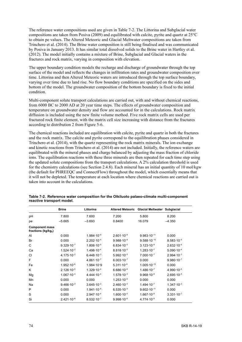
74 SKB R-14-19

The reference water compositions used are given in Table 7-2. The Littorina and Subglacial water compositions are taken from Posiva (2009) and equilibrated with calcite, pyrite and quartz at 25°C to obtain pe values. The Altered Meteoric and Glacial Meltwater compositions are taken from Trinchero et al. (2014). The Brine water composition is still being finalised and was communicated by Posiva in January 2013. It has similar total dissolved solids to the Brine water in Hartley et al. (2012). The model initially contains a mixture of Brine, Subglacial and Glacial waters in the fractures and rock matrix, varying in composition with elevation.

The upper boundary condition models the recharge and discharge of groundwater through the top surface of the model and reflects the changes in infiltration rates and groundwater composition over time. Littorina and then Altered Meteoric waters are introduced through the top surface boundary, varying over time due to land rise. No flow boundary conditions are specified on the sides and bottom of the model. The groundwater composition of the bottom boundary is fixed to the initial condition.

Multi-component solute transport calculations are carried out, with and without chemical reactions, from 6000 BC to 2000 AD at 20 year time steps. The effects of groundwater composition and temperature on groundwater density and flow are accounted for in the calculations. Rock matrix diffusion is included using the new finite volume method. Five rock matrix cells are used per fractured rock finite element, with the matrix cell size increasing with distance from the fractures according to distribution 2 from Figure 5-6.

The chemical reactions included are equilibration with calcite, pyrite and quartz in both the fractures and the rock matrix. The calcite and pyrite correspond to the equilibration phases considered in Trinchero et al. (2014), with the quartz representing the rock matrix minerals. The ion exchange and kinetic reactions from Trinchero et al. (2014) are not included. Initially, the reference waters are equilibrated with the mineral phases and charge balanced by adjusting the mass fraction of chloride ions. The equilibration reactions with these three minerals are then repeated for each time step using the updated solute compositions from the transport calculations. A 2% calculation threshold is used for the chemistry calculations (see Section 2.4.8). Each mineral has an initial quantity of 10 mol/kgw (the default for PHREEQC and ConnectFlow) throughout the model, which essentially means that it will not be depleted. The temperature at each location where chemical reactions are carried out is taken into account in the calculations.

Table 7-2. Reference water composition for the Olkiluoto palaeo-climate multi-component reactive transport model.

Brine Littorina Altered Meteoric Glacial Meltwater Subglacial

pH 7.800 7.600 7.200 5.800 8.200pe –5.665 –3.693 0.8400 16.079 –4.350

Component mass fractions (kg/kgs)Al 0.000 1.984∙10–9 2.601∙10–9 9.983∙10–11 0.000Br 0.000 2.202∙10–5 9.988∙10–8 9.588∙10–10 8.583∙10–5

C 9.329∙10–7 1.806∙10–5 6.834∙10–5 3.123∙10–8 2.632∙10–6

Ca 1.524∙10–2 1.498∙10–4 8.818∙10–5 1.283∙10–7 5.090∙10–4

Cl 4.175∙10–2 6.448∙10–3 5.992∙10–5 7.000∙10–7 2.994∙10–3

F 0.000 4.861∙10–7 6.003∙10–7 0.000 9.980∙10–7

Fe 1.952∙10–6 1.984∙10–9 5.311∙10–6 1.005∙10–10 0.000K 2.126∙10–5 1.329∙10–4 6.686∙10–6 1.486∙10–7 4.990∙10–6

Mg 1.067∙10–4 4.444∙10–4 1.578∙10–5 9.968∙10–8 2.695∙10–5

Mn 0.000 0.000 1.253∙10–6 0.000 0.000Na 9.466∙10–3 3.645∙10–3 2.460∙10–5 1.494∙10–7 1.347∙10–3

P 0.000 1.941∙10–8 6.535∙10–9 9.602∙10–11 0.000S 0.000 2.947∙10–4 1.600∙10–5 1.667∙10–8 3.331∙10–7

Si 2.421∙10–6 8.532∙10–7 9.998∙10–6 4.774∙10–9 0.000

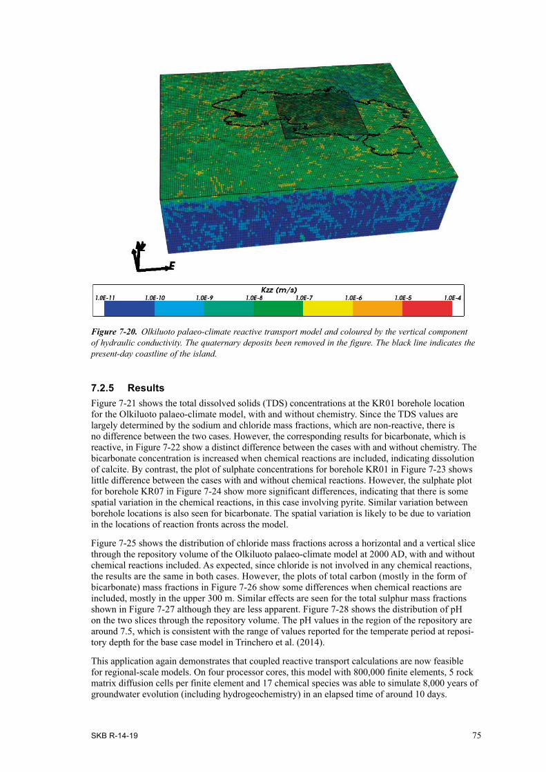
SKB R-14-19 75

7.2.5 ResultsFigure 7-21 shows the total dissolved solids (TDS) concentrations at the KR01 borehole location for the Olkiluoto palaeo-climate model, with and without chemistry. Since the TDS values are largely determined by the sodium and chloride mass fractions, which are non-reactive, there is no difference between the two cases. However, the corresponding results for bicarbonate, which is reactive, in Figure 7-22 show a distinct difference between the cases with and without chemistry. The bicarbonate concentration is increased when chemical reactions are included, indicating dissolution of calcite. By contrast, the plot of sulphate concentrations for borehole KR01 in Figure 7-23 shows little difference between the cases with and without chemical reactions. However, the sulphate plot for borehole KR07 in Figure 7-24 show more significant differences, indicating that there is some spatial variation in the chemical reactions, in this case involving pyrite. Similar variation between borehole locations is also seen for bicarbonate. The spatial variation is likely to be due to variation in the locations of reaction fronts across the model.

Figure 7-25 shows the distribution of chloride mass fractions across a horizontal and a vertical slice through the repository volume of the Olkiluoto palaeo-climate model at 2000 AD, with and without chemical reactions included. As expected, since chloride is not involved in any chemical reactions, the results are the same in both cases. However, the plots of total carbon (mostly in the form of bicarbonate) mass fractions in Figure 7-26 show some differences when chemical reactions are included, mostly in the upper 300 m. Similar effects are seen for the total sulphur mass fractions shown in Figure 7-27 although they are less apparent. Figure 7-28 shows the distribution of pH on the two slices through the repository volume. The pH values in the region of the repository are around 7.5, which is consistent with the range of values reported for the temperate period at reposi-tory depth for the base case model in Trinchero et al. (2014).

This application again demonstrates that coupled reactive transport calculations are now feasible for regional-scale models. On four processor cores, this model with 800,000 finite elements, 5 rock matrix diffusion cells per finite element and 17 chemical species was able to simulate 8,000 years of groundwater evolution (including hydrogeochemistry) in an elapsed time of around 10 days.

Figure 7‑20. Olkiluoto palaeo-climate reactive transport model and coloured by the vertical component of hydraulic conductivity. The quaternary deposits been removed in the figure. The black line indicates the present-day coastline of the island.

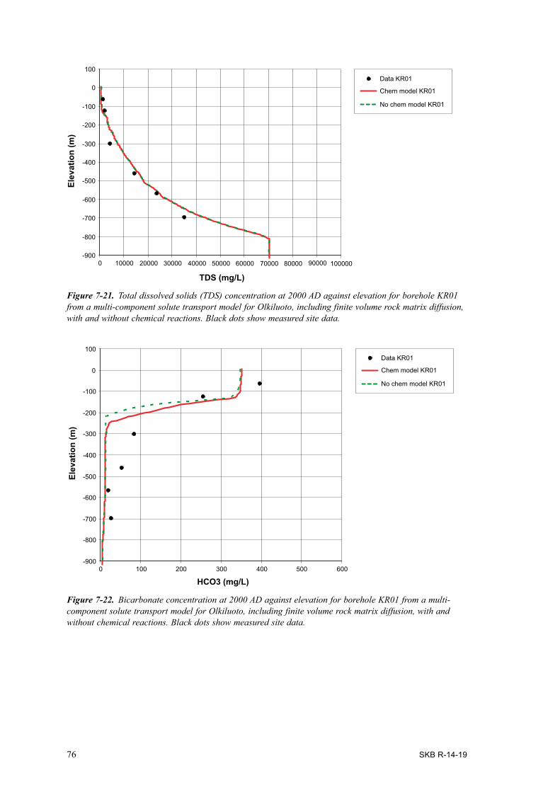
76 SKB R-14-19

Figure 7‑21. Total dissolved solids (TDS) concentration at 2000 AD against elevation for borehole KR01 from a multi-component solute transport model for Olkiluoto, including finite volume rock matrix diffusion, with and without chemical reactions. Black dots show measured site data.

Figure 7‑22. Bicarbonate concentration at 2000 AD against elevation for borehole KR01 from a multi-component solute transport model for Olkiluoto, including finite volume rock matrix diffusion, with and without chemical reactions. Black dots show measured site data.

-900

-800

-700

-600

-500

-400

-300

-200

-100

0

100

0 10000 20000 30000 40000 50000 60000 70000 80000 90000 100000

TDS (mg/L)

Elev

atio

n (m

)Data KR01

Chem model KR01

No chem model KR01

Data KR01

Chem model KR01

No chem model KR01

-900

-800

-700

-600

-500

-400

-300

-200

-100

0

100

0 100 200 300 400 500 600

HCO3 (mg/L)

Elev

atio

n (m

)

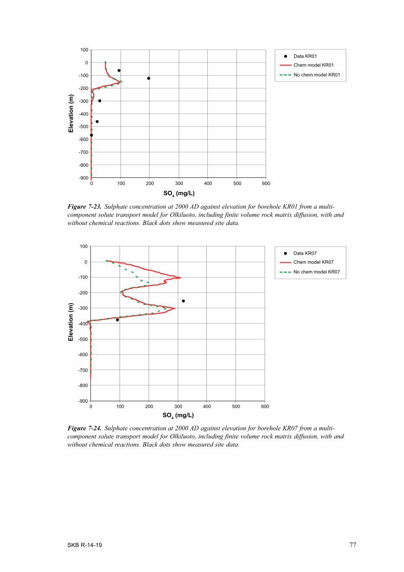
SKB R-14-19 77

Figure 7‑23. Sulphate concentration at 2000 AD against elevation for borehole KR01 from a multi-component solute transport model for Olkiluoto, including finite volume rock matrix diffusion, with and without chemical reactions. Black dots show measured site data.

Figure 7‑24. Sulphate concentration at 2000 AD against elevation for borehole KR07 from a multi-component solute transport model for Olkiluoto, including finite volume rock matrix diffusion, with and without chemical reactions. Black dots show measured site data.

Data KR01

Chem model KR01

No chem model KR01

-900

-800

-700

-600

-500

-400

-300

-200

-100

0

100

0 100 200 300 400 500 600

SO4 (mg/L)

Elev

atio

n (m

)

Data KR07

Chem model KR07

No chem model KR07

-900

-800

-700

-600

-500

-400

-300

-200

-100

0

100

0 100 200 300 400 500 600

SO4 (mg/L)

Elev

atio

n (m

)

78 SKB R-14-19

Figure 7‑25. Vertical and horizontal slices, coloured by chloride mass fraction, taken through the repository volume of the Olkiluoto palaeo-climate model at 2000 AD with chemical reactions (bottom) and without chemical reactions (top). The horizontal slice is at repository depth (–410 m). The vertical slice is taken through the centre of the repository volume and extends northwest to southeast. The locations of the repository structures are shown in black for illustration, although they are not present in the model. The present-day coastline of the island is also shown in black.

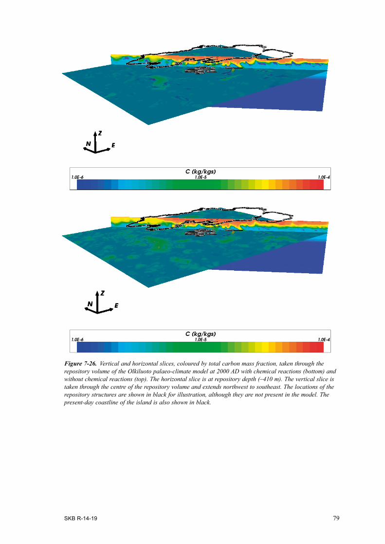
SKB R-14-19 79

Figure 7‑26. Vertical and horizontal slices, coloured by total carbon mass fraction, taken through the repository volume of the Olkiluoto palaeo-climate model at 2000 AD with chemical reactions (bottom) and without chemical reactions (top). The horizontal slice is at repository depth (–410 m). The vertical slice is taken through the centre of the repository volume and extends northwest to southeast. The locations of the repository structures are shown in black for illustration, although they are not present in the model. The present-day coastline of the island is also shown in black.

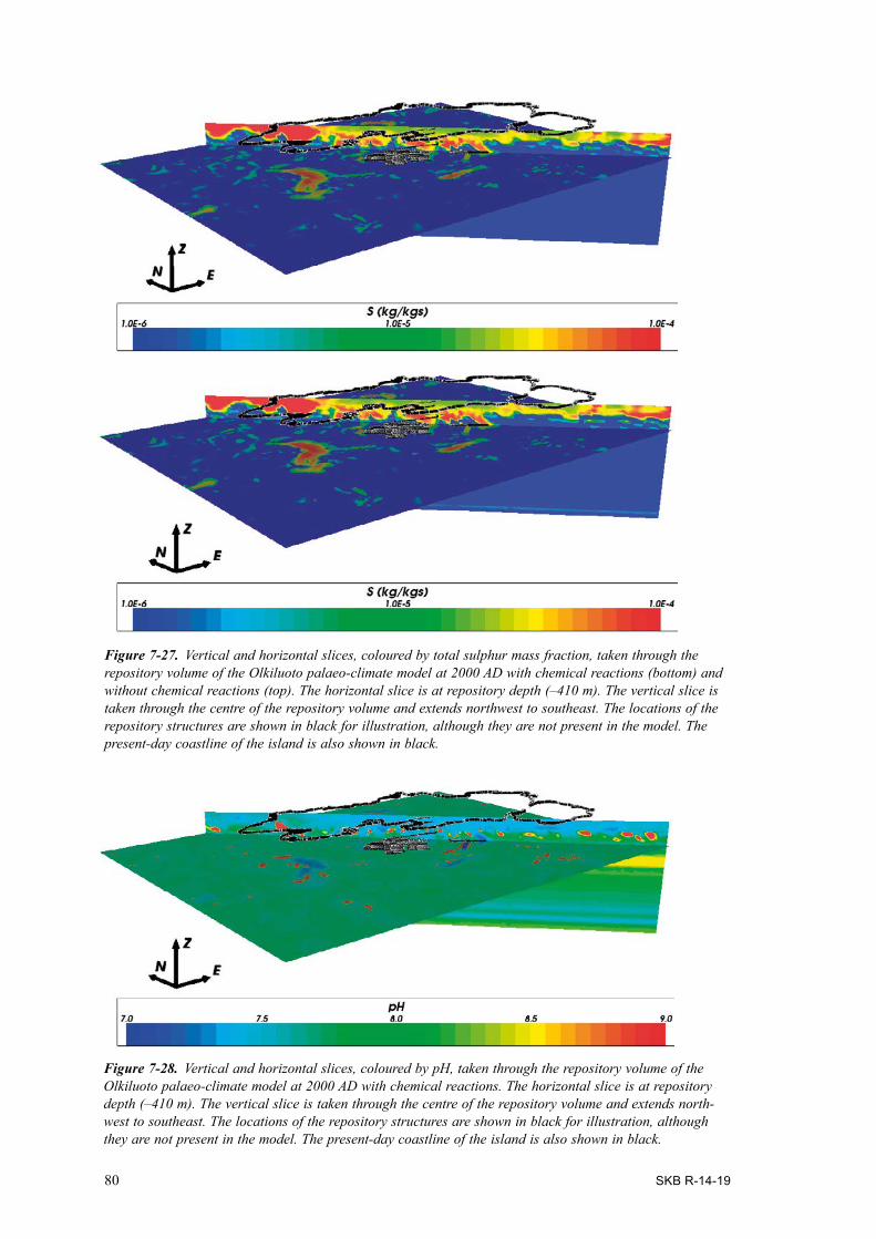
80 SKB R-14-19

Figure 7‑28. Vertical and horizontal slices, coloured by pH, taken through the repository volume of the Olkiluoto palaeo-climate model at 2000 AD with chemical reactions. The horizontal slice is at repository depth (–410 m). The vertical slice is taken through the centre of the repository volume and extends north-west to southeast. The locations of the repository structures are shown in black for illustration, although they are not present in the model. The present-day coastline of the island is also shown in black.

Figure 7‑27. Vertical and horizontal slices, coloured by total sulphur mass fraction, taken through the repository volume of the Olkiluoto palaeo-climate model at 2000 AD with chemical reactions (bottom) and without chemical reactions (top). The horizontal slice is at repository depth (–410 m). The vertical slice is taken through the centre of the repository volume and extends northwest to southeast. The locations of the repository structures are shown in black for illustration, although they are not present in the model. The present-day coastline of the island is also shown in black.

SKB R-14-19 81

8 Conclusions

A facility has been implemented in ConnectFlow to carry out chemical reaction calculations during multi-component solute transport simulations in an equivalent continuous porous medium (ECPM) representation of fractured rock, including rock matrix diffusion. The chemical reaction calculations are carried out for each time step using the iPhreeqc library, which provides an interface to the internationally recognised PHREEQC geochemical software. The reactions currently implemented in ConnectFlow include equilibration with mineral phases and ion exchange reactions. The implemen-tation allows for a flexible, spatially varying, specification of solute compositions, mineral quantities and ion exchange quantities. ConnectFlow is able to track the quantities of these species as they vary due to transport or chemistry calculations, which can then be exported for visualisation and analysis. A new method of modelling rock matrix diffusion has been implemented to allow chemical reactions to be efficiently combined with diffusion processes in the rock matrix, thus allowing an important class of physical situations to be modelled.

Verification by comparison to the Phast and TOUGHREACT software products shows that the ConnectFlow implementation is able to accurately represent coupled solute transport and chemical reactions under a variety of situations. In particular, ConnectFlow is able to almost exactly reproduce the results from Phast for all of the cases considered. The agreement between ConnectFlow and TOUGHREACT is reasonable, although there are differences due to differences in the numerical methods used by the two software products.

Computational efficiency is a critical consideration for reactive transport simulations and has historically been a controlling factor on the scale and types of situations that can be modelled. The implementation within ConnectFlow has therefore been focused on efficiency. Additionally, parallelisation has been applied to key parts of the calculations in terms of performance, namely the chemistry calculations and the equation assembly, so that the multi-processor capabilities of modern computers can be fully utilised to significantly improve run times. Also calculation thresholds can be used to restrict chemistry calculations to those parts of the model that are actually changing as a result of solute transport.

This work has addressed much of the basic functionality and practical constraints in performing large scale transient reactive transport calculations. However, further work remains to broaden the range of reactions than can be provided from the ConnectFlow interface and to make further efficiencies. For instance, the following facilities have not been included in the current implementation, but could be readily added in future developments:

• Kinetic reactions.

• Surface complexation.

• Solid solutions.

• Pore clogging in the rock matrix.

• Export of non-master species for the rock matrix.

• Multiple sequential iteration of groundwater flow, transport and chemistry.

A range of applications are available to the new reactive transport capability within ConnectFlow. One of those is to couple chemical reactions with the palaeo-climate calculations carried out for Forsmark and Olkiluoto as part of the site descriptive modelling and safety assessment calculations. Chemical equilibration with some of the predominant minerals present at these sites during the evolution of the groundwater composition during the last several thousand years provides insight into the processes important in determining the present day distribution of solutes. At Forsmark, advective transport, mixing of groundwaters and rock matrix diffusion were found to be the pre-dominant processes, with the chemical reactions considered to have only a minor impact on present day groundwater composition. For Olkiluoto, the simulations suggest that the effects of chemical reactions are more apparent and may play a more significant role in determining the chemical condi-tions in the site area.

82 SKB R-14-19

Other possible applications include modelling the impact of leachates from cementitious materials (used as part of repository construction) during the operational and post-closure phases of the repositories. For these situations, mixing with groundwater, rock matrix diffusion and chemical reac-tions are important processes in buffering the potentially high pH plumes that are associated with the cement leachates, which can otherwise have negative consequences for repository safety functions. ConnectFlow now has the capability to model all these processes in combination and is thus able to simulate the consequences of these scenarios at a range of scales.

Another application would be to model radionuclide transport taking into account relevant chemical processes such as precipitation/dissolution, ion exchange, surface complexes and solid solutions (the latter two processes are still to be implemented in the ConnectFlow interface to iPhreeqc). This would allow the effects of changing chemical conditions, such as salinity and pH, to be fully accounted for in considering the retardation of radionuclides (Posiva 2012c).

SKB R-14-19 83

References

SKB’s (Svensk Kärnbränslehantering AB) publications can be found at www.skb.se/publications.

AMEC, 2012. CONNECTFLOW Release 10.4 Technical summary document. AMEC/ENV/CONNECTFLOW/15, AMEC, UK.

Carrera J, Sánchez-Vila X, Benet I, Medina A, Galarza G, Guimerà J, 1998. On matrix diffu-sion: formulations, solution methods and qualitative effects. Hydrogeology Journal 6, 178–190.

Charlton S R, Parkhurst D L, 2011. Modules based on the geochemical model PHREEQC for use in scripting and programming languages. Computers & Geosciences 37, 1653–1663.

Crawford J, 2008. Bedrock transport properties Forsmark. Site descriptive modelling, SDM-Site Forsmark. SKB R-08-48, Svensk Kärnbränslehantering AB.

Ewart F T, Sharland S M, Tasker P W, 1985. The chemistry of the near-field environment. In Werme L O (ed). Scientific basis for nuclear waste management IX: symposium held in Stockholm, Sweden, 9–11 September 1985. Pittsburgh, PA: Materials Research Society. (Materials Research Society Symposium Proceedings 50), 539–546.

Follin S, 2008. Bedrock hydrogeology Forsmark. Site descriptive modelling, SDM-Site Forsmark. SKB R-08-95, Svensk Kärnbränslehantering AB.

Grandia F, Galíndez J-M, Arcos D, Molinero J, 2010. Quantitative modelling of the degradation processes of cement grout. Project CEMMOD. SKB TR-10-25, Svensk Kärnbränslehantering AB.

Hartley L, Joyce S, 2013. Approaches and algorithms for groundwater flow modeling in support of site investigations and safety assessment of the Forsmark site, Sweden. Journal of Hydrology 500, 200–216.

Hartley L, Appleyard P, Baxter S, Hoek J, Roberts D, Swan D, 2012. Development of a hydro-geological discrete fracture network model for the Olkiluoto site descriptive model 2011. Posiva Working Report 2012-32, Posiva Oy.

Hartley L, Hoek J, Swan D, Appleyard P, Baxter S, Roberts D, Simpson T, 2013. Hydrogeological modelling for assessment of radionuclide release scenarios for the repository system 2012. Posiva Working Report 2012-42, Posiva Oy, Finland.

Hedenström A, Sohlenius G, Strömgren M, Brydsten L, Nyman H, 2008. Depth and stratig-raphy of regolith at Forsmark. Site desprictive modelling, SDM-Site Forsmark. SKB R-08-07, Svensk Kärnbränslehantering AB.

Hoch A R, Jackson C P, 2004. Rock-matrix diffusion in transport of salinity. Implementation in CONNECTFLOW. SKB R-04-78, Svensk Kärnbränslehantering AB.

Jackson C P, Hoch A R, Todman S, 2000. Self-consistency of a heterogeneous continuum porous medium representation of a fractured medium. Water Resources. Research 36, 189–202.

Joyce S, Simpson T, Hartley L, Applegate D, Hoek J, Jackson P, Swan D, Marsic N, Follin S, 2010. Groundwater flow modelling of periods with temperate climate conditions – Forsmark. SKB R-09-20, Svensk Kärnbränslehantering AB.

Laaksoharju M, Smellie J, Tullborg E-L, Gimeno M, Hallbeck L, Molinero J, Waber N, 2008. Bedrock hydrogeochemistry Forsmark. Site descriptive modelling, SDM-Site Forsmark. SKB R-08-47, Svensk Kärnbränslehantering AB.

Löfgren M, Sidborn M, 2010. Statistical analysis of results from the quantitative mapping of fracture minerals in Forsmark. Site descriptive modelling – complementary studies. SKB R-09-30, Svensk Kärnbränslehantering AB.

Löfman J, Karvonen T, 2012. Simulations of hydrogeological evolution at Olkiluoto. Posiva Working Report 2012-35, Posiva Oy, Finland.

Millero F J, 1970. Apparent and partial molal volume of aqueous sodium chloride solutions at various temperatures. The Journal of Physical Chemistry 74, 356–362.

84 SKB R-14-19

Molinero J, Raposo J R, Galíndez J M, Arcos D, Guimerà J, 2008. Coupled hydrogeological and reactive transport modelling of the Simpevarp area (Sweden). Applied Geochemistry 23, 1957–1981.

Monnin C, 1994. Density calculation and concentration scale conversions for natural waters. Computers & Geosciences 20, 1435–1445.

Neretnieks I, 1980. Diffusion in the rock matrix: an important factor in radionuclide retardation? Journal of Geophysical Research 85, 4379–4397.

Parkhurst D L, Appelo C A J, 1999. User’s guide to PHREEQC (version 2): a computer program for speciation, batch-reaction, one-dimensional transport, and inverse geochemical calculations. Water-Resources Investigations Report 99-4259, U.S. Geological Survey, Denver, Colorado.

Parkhurst D L, Kipp K L, Charlton S R, 2010. PHAST Version 2: a program for simulating groundwater flow, solute transport, and multicomponent geochemical reactions. Techniques and Methods 6-A35, U.S. Geological Survey, Denver, Colorado.

Pitzer K S, 1991. Ion interaction approach: theory and data correlation. In Pitzer K S (ed). Activity coefficients in electrolyte solutions. 2nd ed. Boca Raton, FL: CRC Press, 75–154.

Plummer L N, Parkhurst D L, Fleming G W, Dunkle S A, 1998. A computer program incor-porating Pitzer’s equations for calculation of geochemical reactions in brines. Water-Resources Investigations Report 88-4153, U.S. Geological Survey, Denver, Colorado.

Posiva, 2009. Olkiluoto Site Description 2008. Posiva 2009-01, Posiva Oy, Finland.

Posiva, 2010. Nuclear waste management at Olkiluoto and Loviisa power plants review of current status and future plans for 2010–2012. Posiva TKS-2009, Posiva Oy, Finland.

Posiva, 2011. Olkiluoto site description 2011. Posiva 2011-02, Posiva Oy, Finland.

Posiva, 2012a. Safety case for the disposal of spent nuclear fuel at Olkiluoto – Performance assess-ment 2012. Posiva 2012-04, Posiva Oy, Finland.

Posiva, 2012b. Safety Case for the Disposal of Spent Nuclear Fuel at Olkiluoto – Description of the disposal system 2012. Posiva 2012-05, Posiva Oy, Finland.

Posiva, 2012c. Safety case for the disposal of spent nuclear fuel at Olkiluoto – Assessment of radionuclide release scenarios for the repository system 2012. Posiva 2012-09, Posiva Oy, Finland.

Pruess K, Oldenburg C, Moridis G J, 1999. TOUGH2 user’s guide, version 2.0. Report LBNL-43134, Lawrence Berkeley National Laboratory, Berkeley, California.

Rhén I, Follin S, Hermanson J, 2003. Hydrological Site Descriptive Model – a strategy for its development during Site Investigations. SKB R-03-08, Svensk Kärnbränslehantering AB.

Rhén I, Forsmark T, Hartley L, Joyce S, Roberts D, Gylling B, Marsic N, 2009. Bedrock hydro-geology: model testing and synthesis. Site descriptive modelling, SDM-Site Laxemar. SKB R-08-91, Svensk Kärnbränslehantering AB.

Saaltink M W, Carrera J, Ayora C, 2001. On the behavior of approaches to simulate reactive transport. Journal of Contaminant Hydrology 48, 213–235.

Salas J, Gimeno M J, Auqué L, Molinero J, Gómez J, Juárez I, 2010. SR-Site – hydrogeochemi-cal evolution of the Forsmark site. SKB TR-10-58, Svensk Kärnbränslehantering AB.

Sidborn M, Marsic N, Crawford J, Joyce S, Hartley L, Idiart A, de Vries L M, Maia F, Molinero J, Svensson U, Vidstrand P, Alexander R, 2014. Potential alkaline conditions for deposi-tion holes of a repository in Forsmark as a consequence of OPC grouting. Revised final report after review. SKB R-12-17, Svensk Kärnbränslehantering AB.

Sigg L, 2000. Redox potential measurements in natural waters: significance, concepts and problems. In Schüring J, Schulz H D, Fischer W R, Böttcher J, Duijnisveld W H M (eds). Redox: fundamen-tals, processes and applications. Berlin: Springer, 1–12.

SKB, 2008. Site description of Forsmark at completion of the site investigation phase. SDM-Site Forsmark. SKB TR-08-05, Svensk Kärnbränslehantering AB.

SKB, 2010a. Climate and climate-related issues for the safety assessment SR-Site. SKB TR-10-49, Svensk Kärnbränslehantering AB.

SKB R-14-19 85

SKB, 2010b. RD&D programme 2010. Programme for research, development and demonstra-tion of methods for the management and disposal of nuclear waste. SKB TR-10-63, Svensk Kärnbränslehantering AB.

SKB, 2011. Long-term safety for the final repository for spent nuclear fuel at Forsmark. Main report of the SR-Site project. SKB TR-11-01, Svensk Kärnbränslehantering AB.

Smellie J, Tullborg E-L, Nilsson A-C, Sandström B, Waber N, Gimeno M, Gascoyne M, 2008. Explorative analysis of major components and isotopes. SDM-Site Forsmark. SKB R-08-84, Svensk Kärnbränslehantering AB.

SSM, 2011. Granskning och utvärdering av SKB:s redovisning av Fud-program 2010. Rapport 2011:10, Strålsäkerhetsmyndigheten (Swedish Radiation Safety Authority). (In Swedish.)

Steefel C I, Lasaga A C, 1994. A coupled model for transport of multiple chemical species and kinetic precipitation/dissolution reactions with applications to reactive flow in single phase hydro-thermal systems. American Journal of Science 294, 529–592.

Thomas L H, 1949. Elliptic problems in linear differential equations over a network. Watson Scientific Computing Laboratory, Columbia University, New York.

Trinchero P, Román-Ross G, Maia F, Molinero J, 2014. Posiva Safety Case. Hydrogeochemical evolution of the Olkiluoto Site. Posiva Working Report. 2014-09, Posiva Oy.

Xu T, Sonnenthal E, Spycher N, Pruess K, 2008. TOUGHREACT User’s guide: a simulation program for non-isothermal multiphase reactive geochemical transport in variably saturated geologic media. Lawrence Berkeley National Laboratory, University of California.

SKB R-14-19 87

Appendix A

Component dependent densityIn ConnectFlow the density of the groundwater can be determined using an empirical relationship based on total salinity, temperature and viscosity. An alternative model for density is presented in Monnin (1994). This gives the density in terms of molalities, based on an expression derived in Pitzer (1991). Using Pitzer’s expression, the density depends in a non-linear fashion on the molalities of the individual species. No temperature dependence is provided by Monnin (1994) for the Pitzer parameters, but in Plummer et al. (1998) the temperature dependence is parameterized.

If Pitzer’s density formulation were to be supported in ConnectFlow, it would be necessary to investigate a compatible viscosity expression as well. In fact, transport may be more sensitive to the viscosity function than to the density expression.

Here, the expressions from Monnin (1994) are paraphrased as well as the sources for the Pitzer parameters to be used. These are used to compare the densities for various SKB reference waters with the value currently used in ConnectFlow.

The set of parameters needed is:

• For each ion, its charge and molar mass (g/mol).

• For each cation and anion pair:- standard partial molal volume (cm3/mol),- four parameters in the Pitzer expression (β0, β1, β2, C).

The standard partial molal volume is the partial molal volume in pure water. The set of ions consid-ered in Monnin (1994) are Na+, K+, Ca2+, Mg2+, Cl–, SO42–, HCO3

– and CO32–. The values quoted in

Appendix 1 of Monnin (1994) are used here, plus values for Br– obtained from Millero (1970). The Pitzer parameters are taken from Plummer et al. (1998). There seems to be a different scaling used in Monnin (1994), so the ratio between equivalent results for Cl– between Monnin (1994) and Plummer et al. (1998) is used to rescale the Br– values.

The corrected (Monnin 1994) equations are:

V

Mmi

ii∑+=

1000ρ (A-1)

where:

• ρ = density (g/L),

• mi = molality (mol/kgw),

• Mi = molar mass (g/mol),

• V = volume (L).

The volume of solution that contains 1,000g of water is: ∑ ++=

iexiiw VVmvV 01000 (A-2)

where:

• Vi0 = standard partial molal volume of solute i [cm3/mol],

• vw = specific volume of pure water (cm3/g) = 1/0.9970449 (cm3/g) at 25°C.

∑∑ ∑

++=

c aca

iiicaacDH

ex CzmBmmfRTV ||

212 (A-3)

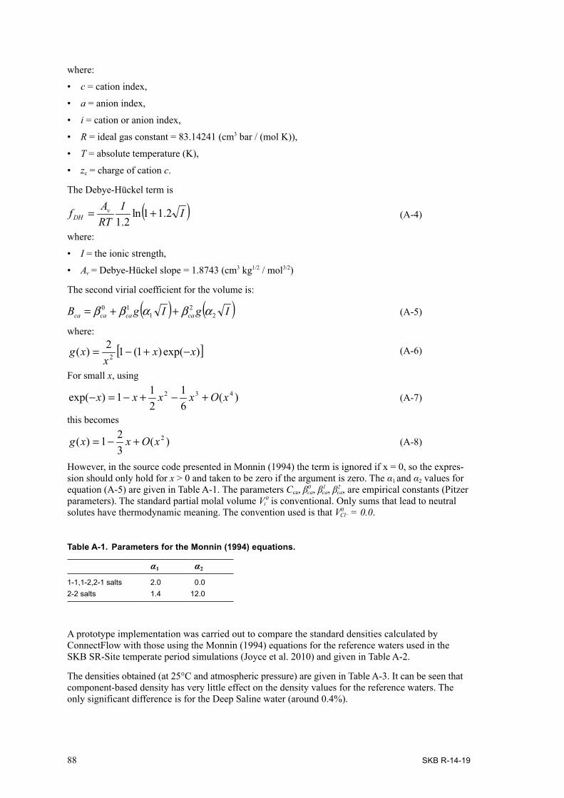
88 SKB R-14-19

where:

• c = cation index,

• a = anion index,

• i = cation or anion index,

• R = ideal gas constant = 83.14241 (cm3 bar / (mol K)),

• T = absolute temperature (K),

• zc = charge of cation c.

The Debye-Hückel term is

( )IIRTAf v

DH 2.11ln2.1

+= (A-4)

where:

• I = the ionic strength,

• Av = Debye-Hückel slope = 1.8743 (cm3 kg1/2 / mol3/2)

The second virial coefficient for the volume is:

( ) ( )IgIgB cacacaca 22

110 αβαββ ++= (A-5)

where:

[ ])exp()1(12)( 2 xxx

xg -+-= (A-6)

For small x, using

)(61

211)exp( 432 xOxxxx +-+-=- (A-7)

this becomes

)(321)( 2xOxxg +-= (A-8)

However, in the source code presented in Monnin (1994) the term is ignored if x = 0, so the expres-sion should only hold for x > 0 and taken to be zero if the argument is zero. The α1 and α2 values for equation (A-5) are given in Table A-1. The parameters Cca, β0

ca, β1ca, β2

ca, are empirical constants (Pitzer parameters). The standard partial molal volume Vi

0 is conventional. Only sums that lead to neutral solutes have thermodynamic meaning. The convention used is that V0

Cl– = 0.0.

Table A-1. Parameters for the Monnin (1994) equations.

α1 α2

1-1,1-2,2-1 salts 2.0 0.02-2 salts 1.4 12.0

A prototype implementation was carried out to compare the standard densities calculated by ConnectFlow with those using the Monnin (1994) equations for the reference waters used in the SKB SR-Site temperate period simulations (Joyce et al. 2010) and given in Table A-2.

The densities obtained (at 25°C and atmospheric pressure) are given in Table A-3. It can be seen that component-based density has very little effect on the density values for the reference waters. The only significant difference is for the Deep Saline water (around 0.4%).

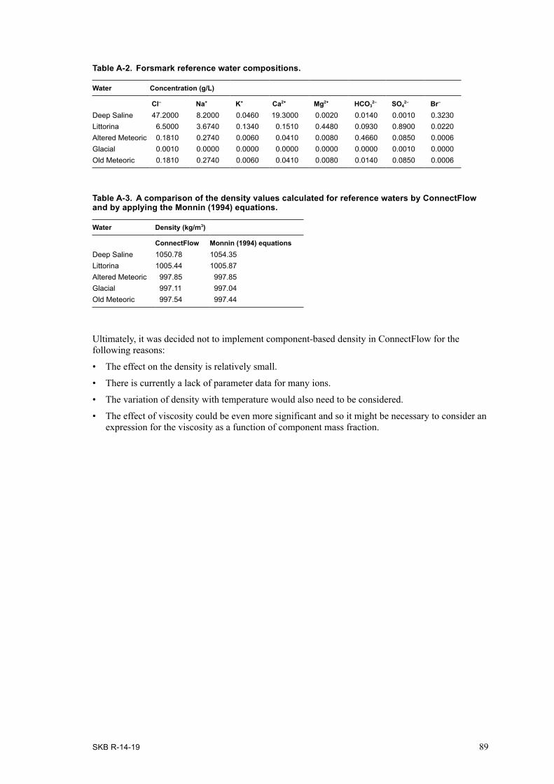
SKB R-14-19 89

Table A-2. Forsmark reference water compositions.

Water Concentration (g/L)

Cl– Na+ K+ Ca2+ Mg2+ HCO32– SO4

2– Br–

Deep Saline 47.2000 8.2000 0.0460 19.3000 0.0020 0.0140 0.0010 0.3230Littorina 6.5000 3.6740 0.1340 0.1510 0.4480 0.0930 0.8900 0.0220Altered Meteoric 0.1810 0.2740 0.0060 0.0410 0.0080 0.4660 0.0850 0.0006Glacial 0.0010 0.0000 0.0000 0.0000 0.0000 0.0000 0.0010 0.0000Old Meteoric 0.1810 0.2740 0.0060 0.0410 0.0080 0.0140 0.0850 0.0006

Table A-3. A comparison of the density values calculated for reference waters by ConnectFlow and by applying the Monnin (1994) equations.

Water Density (kg/m3)

ConnectFlow Monnin (1994) equationsDeep Saline 1050.78 1054.35Littorina 1005.44 1005.87Altered Meteoric 997.85 997.85Glacial 997.11 997.04Old Meteoric 997.54 997.44

Ultimately, it was decided not to implement component-based density in ConnectFlow for the following reasons:

• The effect on the density is relatively small.

• There is currently a lack of parameter data for many ions.

• The variation of density with temperature would also need to be considered.

• The effect of viscosity could be even more significant and so it might be necessary to consider an expression for the viscosity as a function of component mass fraction.

Groundwater flow and reactive transport modelling in … · Den kemiska sammansättningen av...

Documents

Transcript of Groundwater flow and reactive transport modelling in … · Den kemiska sammansättningen av...