Chapter 1

Ground water

If a hole is dug, only the water that flows freely into the hole is groundwater. Since

the air in the hole is at atmospheric pressure, the pressure in the groundwater must

be higher if it is to flow freely into the hole. This is what distinguishes groundwater

from the rest of the underground water.

Definition 1.1. Water, below the surface, at a pressure greater than atmospheric

pressure, which thus flows freely into a hole through interconnected void spaces,

is groundwater.

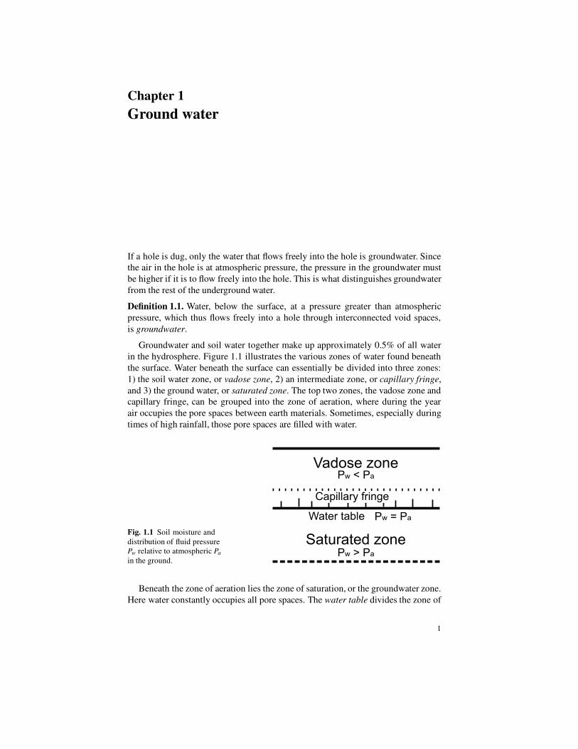
Groundwater and soil water together make up approximately 0.5% of all water

in the hydrosphere. Figure 1.1 illustrates the various zones of water found beneath

the surface. Water beneath the surface can essentially be divided into three zones:

1) the soil water zone, or vadose zone, 2) an intermediate zone, or capillary fringe,

and 3) the ground water, or saturated zone. The top two zones, the vadose zone and

capillary fringe, can be grouped into the zone of aeration, where during the year

air occupies the pore spaces between earth materials. Sometimes, especially during

times of high rainfall, those pore spaces are filled with water.

Fig. 1.1 Soil moisture and

distribution of fluid pressure

Pw relative to atmospheric Pa

in the ground.

Saturated zone

Vadose zone

Capillary fringe

Water table

Pw < Pa

Pw > Pa

Pw = Pa

Beneath the zone of aeration lies the zone of saturation, or the groundwater zone.

Here water constantly occupies all pore spaces. The water table divides the zone of

1

2 1 Ground water

aeration from the zone of saturation. The elevation of the water table is determined

to be where the pore water pressure, Pw, is equal to atmospheric pressure, Pa. The

height of the water table will fluctuate with precipitation, increasing in elevation

during wet periods and decreasing during dry. In general, the water table has an

undulating surface which generally follows the surface topography, but with smaller

relief.

1.1 Porosity

Ground water and soil moisture occur in the cracks, voids, and pore spaces of the

otherwise solid earth materials.

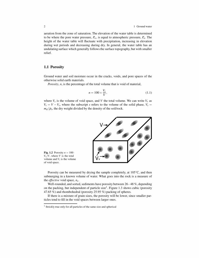
Porosity, n, is the percentage of the total volume that is void of material,

n = 100×Vv

V, (1.1)

where Vv is the volume of void space, and V the total volume. We can write Vv as

Vv = V −Vs, where the subscript s refers to the volume of the solid phase, Vs =md/ρs, the dry weight divided by the density of the soil/rock.

Fig. 1.2 Porosity n = 100 ·

Vv/V , where V is the total

volume and Vv is the volume

of void space.

V

Vv

Porosity can be measured by drying the sample completely, at 105◦C, and then

submerging in a known volume of water. What goes into the rock is a measure of

the effective void space, ne.

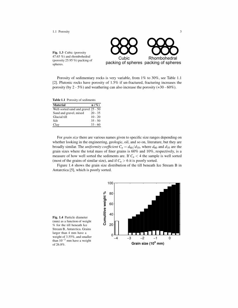
Well-rounded, and sorted, sediments have porosity between 26 - 48 %, depending

on the packing, but independent of particle size1. Figure 1.3 shows cubic (porosity

47.65 %) and rhombohedral (porosity 25.95 %) packing of spheres.

If there is a mixture of grain sizes, the porosity will be lower, since smaller par-

ticles tend to fill in the void spaces between larger ones.

1 Strickly true only for all particles of the same size and spherical

1.1 Porosity 3

Fig. 1.3 Cubic (porosity

47.65 %) and rhombohedral

(porosity 25.95 %) packing of

spheres.

Rhombohedralpacking of spheres

Cubicpacking of spheres

Porosity of sedimentary rocks is very variable, from 1% to 30%, see Table 1.1

[2]. Plutonic rocks have porosity of 1.5% if un-fractured, fracturing increases the

porosity (by 2 - 5%) and weathering can also increase the porosity (+30 - 60%).

Table 1.1 Porosity of sediments

Material n (%)

Well-sorted sand and gravel 25 - 50

Sand and gravel, mixed 20 - 35

Glacial till 10 - 20

Silt 35 - 50

Clay 33 - 60

For grain size there are various names given to specific size ranges depending on

whether looking in the engineering, geologic, oil, and so on, literature, but they are

broadly similar. The uniformity coefficient Cu = d60/d10, where d60 and d10 are the

grain sizes where the total mass of finer grains is 60% and 10%, respectively, is a

measure of how well sorted the sediments are. If Cu < 4 the sample is well sorted

(most of the grains of similar size), and if Cu > 6 it is poorly sorted.

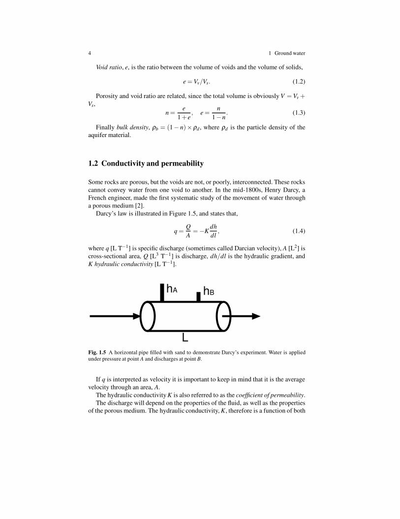
Figure 1.4 shows the grain size distribution of the till beneath Ice Stream B in

Antarctica [5], which is poorly sorted.

Fig. 1.4 Particle diameter

(mm) as a function of weight

% for the till beneath Ice

Stream B, Antarctica. Grains

larger than 4 mm have a

weight of 3.55%, and smaller

than 10−3 mm have a weight

of 26.8%.

−4 −3 −2 −1 00

20

40

60

80

100

Grain size (10x mm)

Cu

mu

liti

ve

weig

ht

%

4 1 Ground water

Void ratio, e, is the ratio between the volume of voids and the volume of solids,

e = Vv/Vs. (1.2)

Porosity and void ratio are related, since the total volume is obviously V = Vv +Vs,

n =e

1 + e, e =

n

1−n. (1.3)

Finally bulk density, ρb = (1− n)×ρd , where ρd is the particle density of the

aquifer material.

1.2 Conductivity and permeability

Some rocks are porous, but the voids are not, or poorly, interconnected. These rocks

cannot convey water from one void to another. In the mid-1800s, Henry Darcy, a

French engineer, made the first systematic study of the movement of water through

a porous medium [2].

Darcy’s law is illustrated in Figure 1.5, and states that,

q =Q

A= −K

dh

dl, (1.4)

where q [L T−1] is specific discharge (sometimes called Darcian velocity), A [L2] is

cross-sectional area, Q [L3 T−1] is discharge, dh/dl is the hydraulic gradient, and

K hydraulic conductivity [L T−1].

L

hA hB

Fig. 1.5 A horizontal pipe filled with sand to demonstrate Darcy’s experiment. Water is applied

under pressure at point A and discharges at point B.

If q is interpreted as velocity it is important to keep in mind that it is the average

velocity through an area, A.

The hydraulic conductivity K is also referred to as the coefficient of permeability.

The discharge will depend on the properties of the fluid, as well as the properties

of the porous medium. The hydraulic conductivity, K, therefore is a function of both

1.3 Capillary forces 5

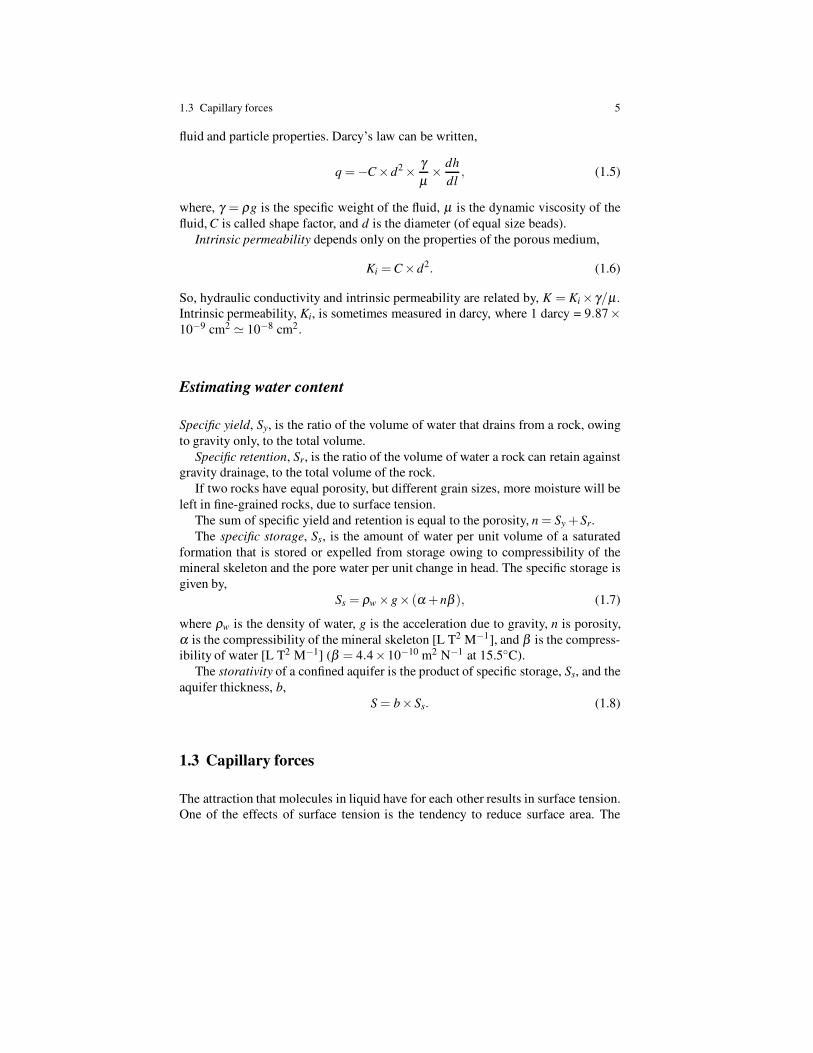
fluid and particle properties. Darcy’s law can be written,

q = −C×d2×

γ

µ×

dh

dl, (1.5)

where, γ = ρg is the specific weight of the fluid, µ is the dynamic viscosity of the

fluid, C is called shape factor, and d is the diameter (of equal size beads).

Intrinsic permeability depends only on the properties of the porous medium,

Ki = C×d2. (1.6)

So, hydraulic conductivity and intrinsic permeability are related by, K = Ki × γ/µ.

Intrinsic permeability, Ki, is sometimes measured in darcy, where 1 darcy = 9.87×

10−9 cm2' 10−8 cm2.

Estimating water content

Specific yield, Sy, is the ratio of the volume of water that drains from a rock, owing

to gravity only, to the total volume.

Specific retention, Sr, is the ratio of the volume of water a rock can retain against

gravity drainage, to the total volume of the rock.

If two rocks have equal porosity, but different grain sizes, more moisture will be

left in fine-grained rocks, due to surface tension.

The sum of specific yield and retention is equal to the porosity, n = Sy +Sr.

The specific storage, Ss, is the amount of water per unit volume of a saturated

formation that is stored or expelled from storage owing to compressibility of the

mineral skeleton and the pore water per unit change in head. The specific storage is

given by,

Ss = ρw ×g× (α +nβ ), (1.7)

where ρw is the density of water, g is the acceleration due to gravity, n is porosity,

α is the compressibility of the mineral skeleton [L T2 M−1], and β is the compress-

ibility of water [L T2 M−1] (β = 4.4×10−10 m2 N−1 at 15.5◦C).

The storativity of a confined aquifer is the product of specific storage, Ss, and the

aquifer thickness, b,

S = b×Ss. (1.8)

1.3 Capillary forces

The attraction that molecules in liquid have for each other results in surface tension.

One of the effects of surface tension is the tendency to reduce surface area. The

6 1 Ground water

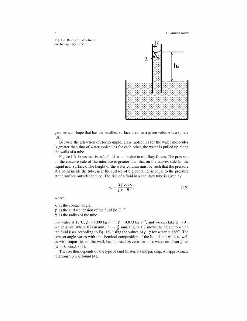
Fig. 1.6 Rise of fluid column

due to capillary force. R

hc

l

geometrical shape that has the smallest surface area for a given volume is a sphere

[3].

Because the attraction of, for example, glass molecules for the water molecules

is greater than that of water molecules for each other, the water is pulled up along

the walls of a tube.

Figure 1.6 shows the rise of a fluid in a tube due to capillary forces. The pressure

on the concave side of the interface is greater than that on the convex side (in the

liquid near surface). The height of the water column must be such that the pressure

at a point inside the tube, near the surface of big container is equal to the pressure

at the surface outside the tube. The rise of a fluid in a capillary tube is given by,

hc =2γ

ρg

cosλ

R, (1.9)

where,

λ is the contact angle,

γ is the surface tension of the fluid [M T−2],

R is the radius of the tube.

For water at 18◦C, ρ ∼ 1000 kg m−3, γ = 0.073 kg s−2, and we can take λ ∼ 0◦,

which gives (where R is in mm), hc = 15R

mm. Figure 1.7 shows the height to which

the fluid rises according to Eq. 1.9, using the values of ρ , γ for water at 18◦C. The

contact angle varies with the chemical composition of the liquid and wall, as well

as with impurities on the wall, but approaches zero for pure water on clean glass

(λ → 0, cosλ ∼ 1).

The rise thus depends on the type of sand (material) and packing. An approximate

relationship was found [4],

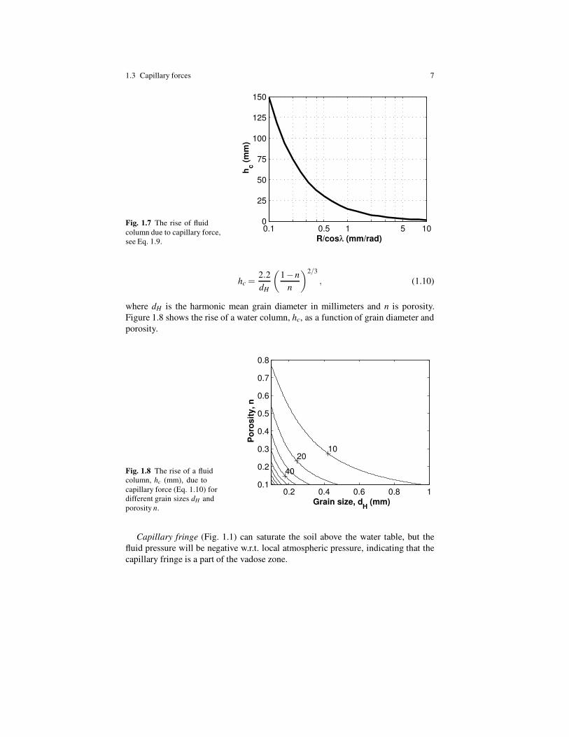
1.3 Capillary forces 7

Fig. 1.7 The rise of fluid

column due to capillary force,

see Eq. 1.9.

0.1 0.5 1 5 100

25

50

75

100

125

150

R/cosλ (mm/rad) h

c (

mm

)

hc =2.2

dH

(

1−n

n

)2/3

, (1.10)

where dH is the harmonic mean grain diameter in millimeters and n is porosity.

Figure 1.8 shows the rise of a water column, hc, as a function of grain diameter and

porosity.

Fig. 1.8 The rise of a fluid

column, hc (mm), due to

capillary force (Eq. 1.10) for

different grain sizes dH and

porosity n.

0.2 0.4 0.6 0.8 10.1

0.2

0.3

0.4

0.5

0.6

0.7

0.8

1020

40

Grain size, dH

(mm)

Po

rosit

y,

n

Capillary fringe (Fig. 1.1) can saturate the soil above the water table, but the

fluid pressure will be negative w.r.t. local atmospheric pressure, indicating that the

capillary fringe is a part of the vadose zone.

8 1 Ground water

1.4 Soil moisture

The zone between the ground surface and down to the water table is called the

vadose zone (unsaturated zone). Water there is held to the soil particles by capillary

forces. The vadose zone (see Figure 1.1) may contain a three-phase system:

• Solid. Mineral grains, and organic material.

• Liquid. Water with dissolved solutes.

• Gaseous. Water vapor, and other gases.

We can write the equation for porosity as,

n = 100× (1−ρb/ρm), (1.11)

where ρb = ms/V is the dry bulk density, subscript s for solid, and ρm = ms/Vs is

the particle density.

The water that is immediately available to plants is a part of the soil water. Soil

water can be sub-divided into three categories: 1) hygroscopic water, 2) capillary

water, and 3) gravitational water.

Hygroscopic water is found as a microscopic film of water surrounding soil par-

ticles. This water is tightly bound to a soil particle by molecular forces so powerful

that it cannot be removed by natural forces. Hygroscopic water is bound to soil par-

ticles by adhesive forces that exceed 31 bars and may be as great as 10 000 bars

(recall that sea level pressure is equal to 1013.2 millibars which is just about 1 bar).

Capillary water is held by cohesive forces between the films of hygroscopic wa-

ter. The binding pressure for capillary water is much less than hygroscopic water.

This water can be removed by air drying, or by plant absorption, but cannot be re-

moved by gravity. Plants extract this water through their roots until the soil capillary

force (force holding water to the particle) is equal to the extractive force of the plant

root. At this point the plant cannot pull water from the plant-rooting zone and it

wilts, called the wilting point.

Definition 1.2. At the wilting point, soil moisture is too tightly bound to the soil

particles for plant roots to be able to withdraw it.

Gravity water is the water moved through the soil by the force of gravity. The

amount of water held in the soil at the point where gravity drainage ceases is called

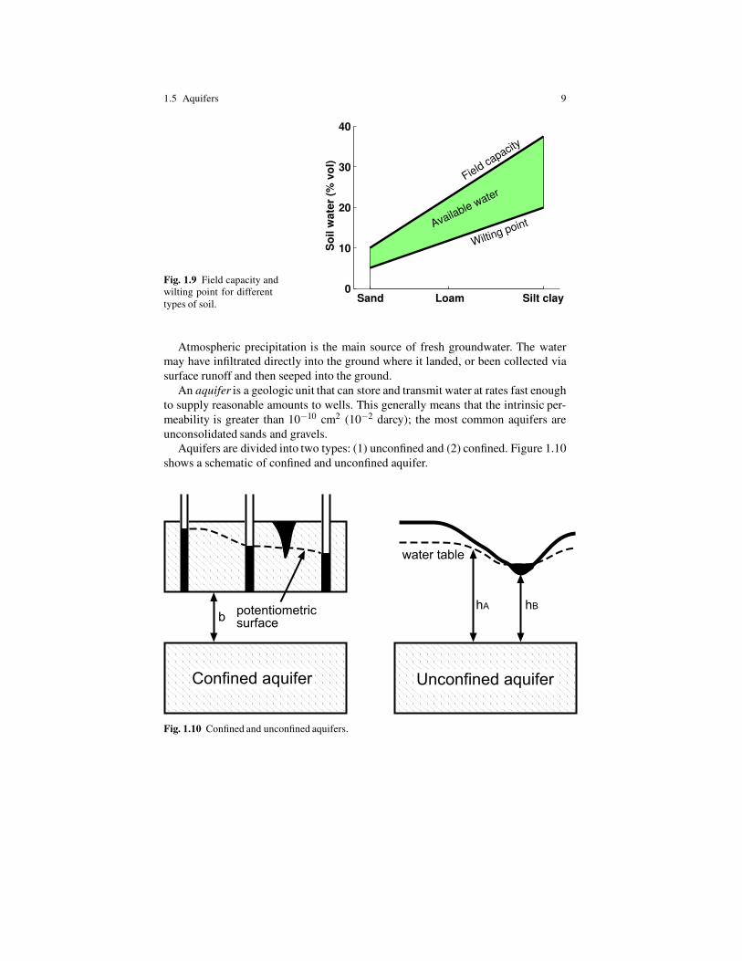
the field capacity of the soil. The amount of water in the soil is controlled by the soil

texture (Figure 1.9).

1.5 Aquifers

Definition 1.3. Aquifers are groundwater-bearing formations that are sufficiently

permeable to transmit and yield water in usable quantities.

1.5 Aquifers 9

Fig. 1.9 Field capacity and

wilting point for different

types of soil.Sand Loam Silt clay

0

10

20

30

40

So

il w

ate

r (%

vo

l)

Wilting point

Field capacity

Available water

Atmospheric precipitation is the main source of fresh groundwater. The water

may have infiltrated directly into the ground where it landed, or been collected via

surface runoff and then seeped into the ground.

An aquifer is a geologic unit that can store and transmit water at rates fast enough

to supply reasonable amounts to wells. This generally means that the intrinsic per-

meability is greater than 10−10 cm2 (10−2 darcy); the most common aquifers are

unconsolidated sands and gravels.

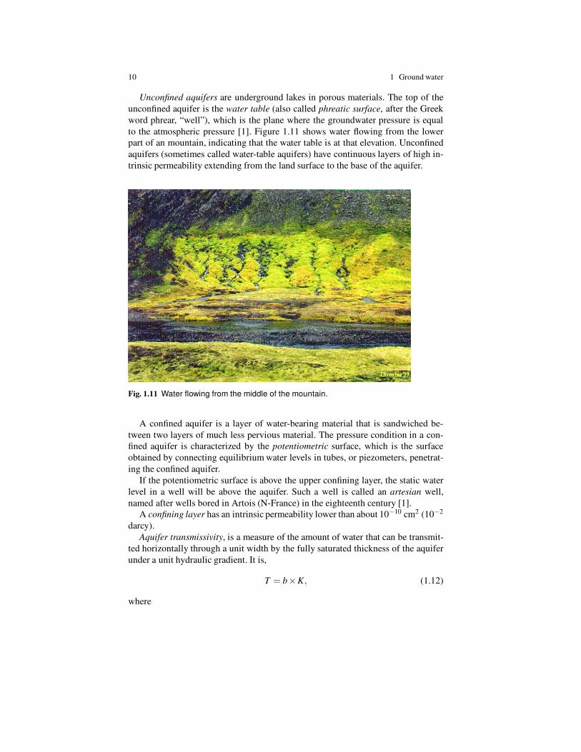
Aquifers are divided into two types: (1) unconfined and (2) confined. Figure 1.10

shows a schematic of confined and unconfined aquifer.

Confined aquifer Unconfined aquifer

water table

hA hB

bpotentiometricsurface

Fig. 1.10 Confined and unconfined aquifers.

10 1 Ground water

Unconfined aquifers are underground lakes in porous materials. The top of the

unconfined aquifer is the water table (also called phreatic surface, after the Greek

word phrear, “well”), which is the plane where the groundwater pressure is equal

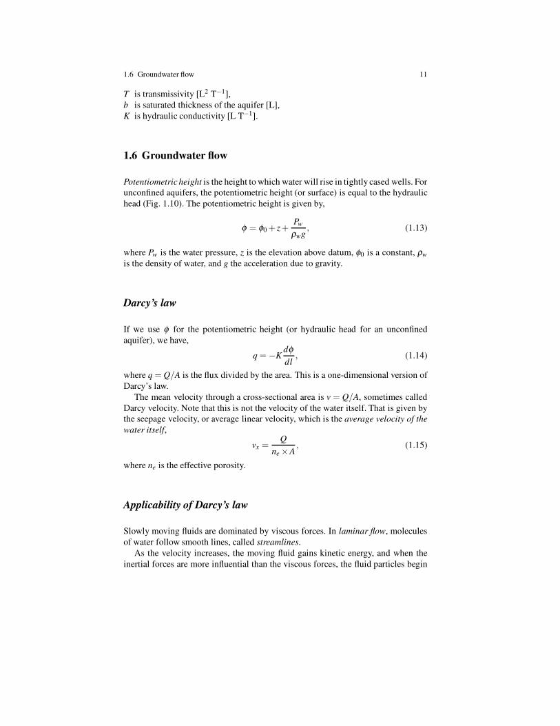
to the atmospheric pressure [1]. Figure 1.11 shows water flowing from the lower

part of an mountain, indicating that the water table is at that elevation. Unconfined

aquifers (sometimes called water-table aquifers) have continuous layers of high in-

trinsic permeability extending from the land surface to the base of the aquifer.

Fig. 1.11 Water flowing from the middle of the mountain.

A confined aquifer is a layer of water-bearing material that is sandwiched be-

tween two layers of much less pervious material. The pressure condition in a con-

fined aquifer is characterized by the potentiometric surface, which is the surface

obtained by connecting equilibrium water levels in tubes, or piezometers, penetrat-

ing the confined aquifer.

If the potentiometric surface is above the upper confining layer, the static water

level in a well will be above the aquifer. Such a well is called an artesian well,

named after wells bored in Artois (N-France) in the eighteenth century [1].

A confining layer has an intrinsic permeability lower than about 10−10 cm2 (10−2

darcy).

Aquifer transmissivity, is a measure of the amount of water that can be transmit-

ted horizontally through a unit width by the fully saturated thickness of the aquifer

under a unit hydraulic gradient. It is,

T = b×K, (1.12)

where

1.6 Groundwater flow 11

T is transmissivity [L2 T−1],

b is saturated thickness of the aquifer [L],

K is hydraulic conductivity [L T−1].

1.6 Groundwater flow

Potentiometric height is the height to which water will rise in tightly cased wells. For

unconfined aquifers, the potentiometric height (or surface) is equal to the hydraulic

head (Fig. 1.10). The potentiometric height is given by,

φ = φ0 + z+Pw

ρwg, (1.13)

where Pw is the water pressure, z is the elevation above datum, φ0 is a constant, ρw

is the density of water, and g the acceleration due to gravity.

Darcy’s law

If we use φ for the potentiometric height (or hydraulic head for an unconfined

aquifer), we have,

q = −Kdφ

dl, (1.14)

where q = Q/A is the flux divided by the area. This is a one-dimensional version of

Darcy’s law.

The mean velocity through a cross-sectional area is v = Q/A, sometimes called

Darcy velocity. Note that this is not the velocity of the water itself. That is given by

the seepage velocity, or average linear velocity, which is the average velocity of the

water itself,

vx =Q

ne ×A, (1.15)

where ne is the effective porosity.

Applicability of Darcy’s law

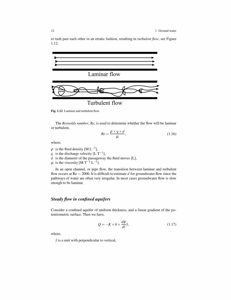
Slowly moving fluids are dominated by viscous forces. In laminar flow, molecules

of water follow smooth lines, called streamlines.

As the velocity increases, the moving fluid gains kinetic energy, and when the

inertial forces are more influential than the viscous forces, the fluid particles begin

12 1 Ground water

to rush past each other in an erratic fashion, resulting in turbulent flow, see Figure

1.12.

Laminar flow

Turbulent flow

Fig. 1.12 Laminar and turbulent flow.

The Reynolds number, Re, is used to determine whether the flow will be laminar

or turbulent,

Re =ρ ×q×d

µ, (1.16)

where,

ρ is the fluid density [M L−3],

q is the discharge velocity [L T−1],

d is the diameter of the passageway the fluid moves [L],

µ is the viscosity [M T−1 L−1].

In an open channel, or pipe flow, the transition between laminar and turbulent

flow occurs at Re ∼ 2000. It is difficult to estimate d for groundwater flow since the

pathways of water are often very irregular. In most cases groundwater flow is slow

enough to be laminar.

Steady flow in confined aquifers

Consider a confined aquifer of uniform thickness, and a linear gradient of the po-

tentiometric surface. Then we have,

Q = −K ×b×dφ

dly, (1.17)

where,

y is a unit with perpendicular to vertical,

1.6 Groundwater flow 13

b is the thickness of the confined aquifer (vertical),

dφ/dl is the slope of the potentiometric surface.

Steady flow in an unconfined aquifer

Now the water table is also the upper boundary of the region of flow (Fig. 1.10),

and from simple geometric arguments the hydraulic gradient will increase in the

direction of flow.

Two assumptions, called Dupuit assumptions, allow us to solve this problem.

They are (1) the hydraulic gradient is equal to the slope of the water table, and (2)

for small water-table gradients, and the streamlines are horizontal.

Starting with Darcy’s equation,

Q = −K ×h×dh

dxy, (1.18)

where h is the saturated thickness of the aquifer. Integrating,

∫ L

0Qdx = −Ky

∫ H2

H1

h dh. (1.19)

After rearrangement, we get,

Q =y

2K

(

H21 −H2

2

L

)

, (1.20)

where

H1 is the head at the origin,

H2 is the head at L,

L is the flow length.

The total discharge at any location must be a constant, no water is coming in or

going out of the system in this case.

To derive the equation for the hydraulic head, when adding or loosing water at

some rate w, we consider the fluxes through an “box”-element. Since the pressure

is zero, we write φ = h. The components of the specific discharge from Darcy’s

equation are,

qi = −K∂ h

∂ xi,

where i = (x,y). Then continuity requires (no storage),

∂

∂ x(qxh)+

∂

∂ y(qyh) = w. (1.21)

We can substitute for qi,

14 1 Ground water

∂

∂ x

(

Kh∂ h

∂ x

)

,

and use the fact that,

h∂ h

∂ x=

1

2

∂ (h2)

∂ x,

which leads to,

−K

(

∂ 2h2

∂ x2+

∂ 2h2

∂ y2

)

= 2w, (1.22)

where w is net addition or loss rate.

If w = 0 we get Laplace equation. If the flow is only in the x-direction, we get

d2h2

dx2= −

2w

K, where x =

{

0, h = H1,L, h = H2,

(1.23)

which gives,

h2 = H21 −

(H21 −H2

2 )x

L+

w

K(L− x)x, (1.24)

where

h is the head at x,

x is the distance from the origin,

L is the distance from the origin to the point where H2 is measured,

w is the recharge rate [L T−1].

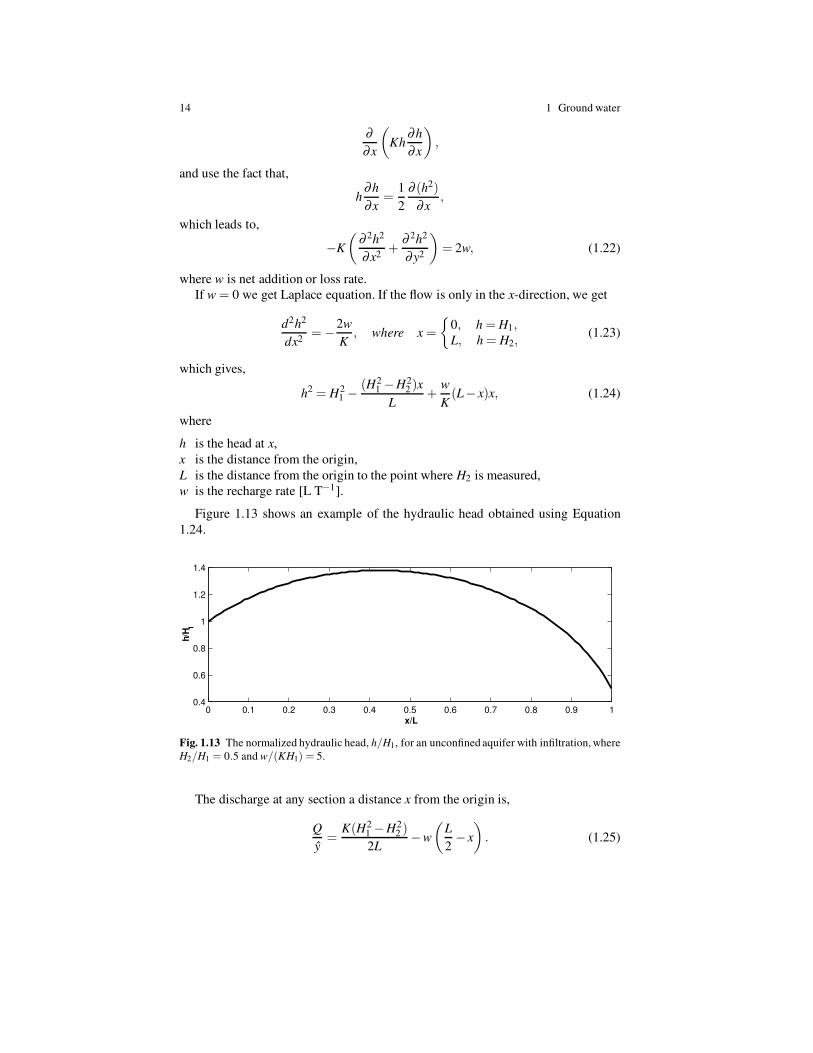
Figure 1.13 shows an example of the hydraulic head obtained using Equation

1.24.

0 0.1 0.2 0.3 0.4 0.5 0.6 0.7 0.8 0.9 10.4

0.6

0.8

1

1.2

1.4

x/L

h/H

1

Fig. 1.13 The normalized hydraulic head, h/H1, for an unconfined aquifer with infiltration, where

H2/H1 = 0.5 and w/(KH1) = 5.

The discharge at any section a distance x from the origin is,

Q

y=

K(H21 −H2

2 )

2L−w

(

L

2− x

)

. (1.25)

1.7 Flow to wells 15

1.7 Flow to wells

The decline in water level around a pumping well is called drawdown.

We can learn about aquifer properties when a well is pumped at a constant rate

and either the stabilzed drawdown, or the rate of drawdown is measured.

These basic assumptions are made:

• The aquifers are homogenous and isotropic, and radially symmetry.

• The wells fully penetrate the aquifers.

• The aquifer is bounded on the bottom by a confining layer.

• Geometry is horizontal of infinite extend.

• The potentiometric surface is horizontal at, and not changing prior to, t = 0, and

all subsequent changes are due to the pumping alone.

• Flow is horizontal and Darcy’s law holds. Water has a constant density (ρ) and

viscosity (µ).

Since we assume radial symmetry it is convenient to use polar coordinates. Two

dimensional flow in a confined aquifer is then given by,

∂ 2φ

∂ r2+

1

r

∂ φ

∂ r=

S

T

∂ φ

∂ t, (1.26)

where (as before), φ is the hydraulic head [L], S is storativity [-] (1.8), T is trans-

missivity [L2T−1] (1.12), t is time [T], and r is radial distance [L] from the pumping

well.

If there is also a (vertical) recharge rate w [L T−1], a term w/T is added to the

left side of (1.26).

Steady State Radial Flow in a Confined Aquifer

Now we look for the steady state solution to (1.26), that is

d2φ

dr2+

1

r

dφ

dr= 0, (1.27)

which has the general solution φ = A lnr +B.

As boundary conditions one could impose certain fixed values for the head for

two values of r. A more realistic set of boundary conditions is to assume a constant

head (φ0) at the outer boundary r = R, and to impose that at the inner boundary a

certain given discharge (Q0) is extracted from the soil. Then the boundary conditions

are,

r =

{

R, φ = φ0,rw, 2πrHqr = −2πTr(dφ/dr) = −Q0,

(1.28)

where Darcy’s law has been used in the form qr = −Kdφ/dr, H is the aquifer

thickness, and the negative sign before Q0 means that the discharge flows in the

16 1 Ground water

negative r direction, that is, towards the well. The solution subject to these boundary

conditions is then,

φ −φ0 =Q0

2πTln

( r

R

)

. (1.29)

Since r < R the logarithm is always negative.

The water level at the well is obtained by setting r = rw in Equation 1.29,

φw = φ0 +Q0

2πTln

(rw

R

)

. (1.30)

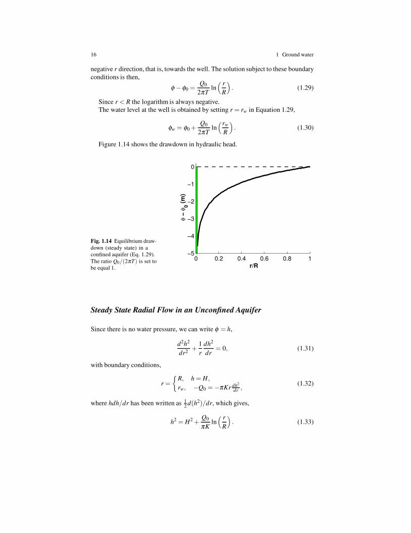
Figure 1.14 shows the drawdown in hydraulic head.

Fig. 1.14 Equilibrium draw-

down (steady state) in a

confined aquifer (Eq. 1.29).

The ratio Q0/(2πT) is set to

be equal 1.

0 0.2 0.4 0.6 0.8 1−5

−4

−3

−2

−1

0

φ −

φ0 (

m)

r/R

Steady State Radial Flow in an Unconfined Aquifer

Since there is no water pressure, we can write φ = h,

d2h2

dr2+

1

r

dh2

dr= 0, (1.31)

with boundary conditions,

r =

{

R, h = H,

rw, −Q0 = −πKr dh2

dr,

(1.32)

where hdh/dr has been written as 12

d(h2)/dr, which gives,

h2 = H2 +Q0

πKln

( r

R

)

. (1.33)

1.8 Problems 17

1.8 Problems

1.1. Compare the surface area of a sphere, cylinder and box, for same volume of

material (same mass, since same density in all cases). Which is smallest?

Hint:

Vb = l×b×h, and Ab = 2× l×b +2×b×h +2× l×h,

Vc = πr2×h, and Ac = 2πr2 +2πrh,

Vs = 4πr3/3, and As = 4πr2.

Put Vb = Vc =Vs (use for instance l,h,b= 1), calculate V with the r you get from

the volume.

1.2. Find the relation between porosity, n, and void ratio, e. That is, start with (1.1)

for n and (1.2) for e, and show that (1.3) holds.

1.3. What is a) an aquifer, and b) the piezometric surface?

1.4. Sketch a) a confined aquifer, and b) an unconfined aquifer.

1.5. Derive Equation (1.11).

1.6. What does the Reynolds-number measure ?

1.7. What is the hydraulic head, φ , at an intermediate distance x between φ1 and φ2,

for a steady flow in a confined aquifer (1.17)?

1.8. For an unconfined aquifer find: a) The distance, d, from the origin where Q = 0

(1.25), i.e. the top of the water table, and b) the maximum hydraulic head (1.24).

Hint: hmax = h(x = d).

Suggested reading

From Fetter [2]:

? Chapters 1-3, for aquifers and soil.

? Chapter 4.6, for Darcy’s law.

? Chapter 4.13, for confined aquifers.

? Chapter 4.14, for unconfinded aquifers.

? Chapter 5.1-5.4, for flow to wells.

? Chapter 6, for soil moisture and ground-water recharge.

References

References

1. Bouwer, H.: Groundwater Hydrology, first edn. McGraw-Hill, New York (1978)

2. Fetter, C.W.: Applied Hydrogeology, fourth edn. Prentice Hall, New Jersey (2001)

3. Price, M.: Introducing groundwater, first edn. Chapman and Hall, London (1985)

4. Todd, D.K.: Ground Water Hydrology, first edn. Wiley International Edition, New York (1959)

5. Tulaczyk, S., Kamb, B., Scherer, R., Engelhardt, H.F.: Sedimentary processes at the base of a

West Antarctic ice stream: Constraints from textural and compositionalproperties of subglacial

debris. Journal of Sedimentary Research 68(3), 487–496 (1998)

19