LUND UNIVERSITY

PO Box 117221 00 Lund+46 46-222 00 00

Ground-truths or Ground-lies? : environmental sampling for remote sensingapplication exemplified by vegetation cover data

Brogaard, Sara; Olafsdottir, Rannveig

1997

Link to publication

Citation for published version (APA):Brogaard, S., & Olafsdottir, R. (1997). Ground-truths or Ground-lies? : environmental sampling for remotesensing application exemplified by vegetation cover data. (Lund electronic reports in physical geography; Vol. 1).Department of Physical Geography, Lund University.

Total number of authors:2

General rightsUnless other specific re-use rights are stated the following general rights apply:Copyright and moral rights for the publications made accessible in the public portal are retained by the authorsand/or other copyright owners and it is a condition of accessing publications that users recognise and abide by thelegal requirements associated with these rights. • Users may download and print one copy of any publication from the public portal for the purpose of private studyor research. • You may not further distribute the material or use it for any profit-making activity or commercial gain • You may freely distribute the URL identifying the publication in the public portal

Read more about Creative commons licenses: https://creativecommons.org/licenses/Take down policyIf you believe that this document breaches copyright please contact us providing details, and we will removeaccess to the work immediately and investigate your claim.

Lund Electronic Reports in Physical GeographyNo. 1, October 1997Department of Physical GeographyLund University, SwedenISSN: 1402 - 9006

Reference: Lund eRep. Phys. Geogr., No. 1, Oct. 1997.

Ground-truths or Ground-lies?

Environmental sampling for remote sensing applicationexemplified by vegetation cover data

Sara Brogaard and Rannveig Ólafsdóttir

Department of Physical GeographyLund UniversitySölvegatan 13

S-223 62 Lund, Sweden

Fax: Int +46 46 222 0321; Tel.: Int + 46 46 222 3622

E-mail: sara.brogaard@natgeo.lu.seandrannveig.olafsdottir@natgeo.lu.se

0. AbstractDuring time of fast development of computer and sensor technology, ground data samplingstrategies have achieved diminished attention in many remote sensing studies. This paperdiscusses the importance of designing an appropriate sampling scheme of ground data collectionfor remote sensing applications. The difficulties of achieving a balance between the size and theerror of the samples are identified. Different techniques of vegetation cover estimations areevaluated to illustrate parts of the proposed sampling design. The study indicates that traditionalmethods of ground data collection for remote sensing applications do not have to result in"ground lies". Determination of a reliable and appropriate sampling scheme for the ground datacollection should be given a more attention when assuring accurate results in remote sensingstudies.

Key words: ground data collection, ground truth, vegetation cover, remote sensing, samplingstrategies

1. IntroductionResource management is making increased use of Geographical Information Systems (GIS). Thisrequires reliable and up-to-date information on the extent, distribution and use of naturalresources in time and space. Remote sensing technology has emerged as a potentially powerfultool for providing information on natural resources at various spatial and temporal resolutions.

Integration of remote sensing data and GIS is facilitated by a number of developments. Thisincludes software and hardware advances as well as price/capability ratios of GIS, theavailability of high-resolution data in digital form, new developments in automated informationextraction, and the use of GIS for spatial and dynamic modeling. What has been given lessconsideration is the accuracy of the input data when integrating data sources in a GIS. Ifincorrectly classified remotely sensed data is included in a database to be used for environmentalmodeling, the results will be uncontrolled error propagation throughout the study. The purposeof the geographical resource information processing is to improve environmental monitoring andmanagement. This can only be achieved if the data are sufficiently reliable and error-free for thepurpose for which they are required.

When using remotely sensed data the sources of errors may result from geometric errors,radiometric errors, a time lag between image acquisition and ground data collection and theactual methods of ground data collection, also referred to as ground truthing. Ground data is usedboth for calibration and the subsequent accuracy assessment of the classified image. Its quality istherefore of fundamental importance. Many researchers (e.g. Hord and Brooner 1976, Hay 1979,Justice and Townshend 1981, Curran and Williamson 1985, 1986, Congalton 1991, Zhou andPilesjö 1996) have questioned the commonly used methods for collecting ground data, evenindicating that inappropriate ground data collection easily may result in "ground lies". It seemsthat during time of fast computer technology and sensor development, sample design hasachieved diminished attention in many remote sensing studies.

This paper aims to highlight the importance of ground data collection for remote sensingpurposes, being aware of the difficulties of achieving a balance between the size and the error ofthe samples. An appropriate sampling scheme, which takes the spatial variation of the studiedpopulation, is discussed. To illustrate parts of the proposed sampling design an example ofground data collection for vegetation cover assessment in a semi-arid rangeland environment ispresented. Different techniques of vegetation cover estimations are also compared.

2. Sampling design considerations

2.1 Importance of designing an appropriate sampling scheme

One of the strengths of remotely sensed data is that it represents a complete spatial population.When computer-derived classifications are used to produce ground cover maps they aregenerally based on ground data collected by the user from selected training areas. The accuracyof the thematic map depends on the user ability to extrapolate successfully from the trainingareas to the whole map area (Thomas and Allcock 1984). Usually the training data set makes upthe first part of the collected ground data, whereas the remaining part is used for accuracyassessment of the classified image.

The sample design is a critical part of the image classification accuracy assessment. The standardform for reporting overall error for each class of the image classification is by the use of an errormatrix. Error matrices represent the number of correctly mapped pixels by comparing grounddata with corresponding results of computer assisted classification. Designing a poor samplingscheme can easily result in significant biases being introduced into the error matrix, which willthen affect the classification accuracy (e.g. Richard 1993, Congalton 1991, Lunetta et. al. 1991).

To ensure that the ground data is representative for the spatial population, a suitable sampledesign has to be chosen. Curran and Williamson (1985) emphasize the importance of therepresentation of ground data, both at the scale of the image to ensure an adequate range of datafor accuracy testing, and at the scale of the pixel to ensure spatial compatibility between ground

data and pixel resolution. Even if complete spatial coverage of a region is provided by remotelysensed imagery, each pixel of the images represents an integration of information, which isconsidered by this approach.

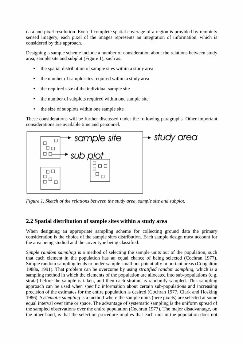
Designing a sample scheme include a number of consideration about the relations between studyarea, sample site and subplot (Figure 1), such as:

• the spatial distribution of sample sites within a study area

• the number of sample sites required within a study area

• the required size of the individual sample site

• the number of subplots required within one sample site

• the size of subplots within one sample site

These considerations will be further discussed under the following paragraphs. Other importantconsiderations are available time and personnel.

Figure 1. Sketch of the relations between the study area, sample site and subplot.

2.2 Spatial distribution of sample sites within a study area

When designing an appropriate sampling scheme for collecting ground data the primaryconsideration is the choice of the sample sites distribution. Each sample design must account forthe area being studied and the cover type being classified.

Simple random samplingis a method of selecting the sample units out of the population, suchthat each element in the population has an equal chance of being selected (Cochran 1977).Simple random sampling tends to under-sample small but potentially important areas (Congalton1988a, 1991). That problem can be overcome by usingstratified random sampling,which is asampling method in which the elements of the population are allocated into sub-populations (e.g.strata) before the sample is taken, and then each stratum is randomly sampled. This samplingapproach can be used when specific information about certain sub-populations and increasingprecision of the estimates for the entire population is desired (Cochran 1977, Clark and Hosking1986).Systematic samplingis a method where the sample units (here pixels) are selected at someequal interval over time or space. The advantage of systematic sampling is the uniform spread ofthe sampled observations over the entire population (Cochran 1977). The major disadvantage, onthe other hand, is that the selection procedure implies that each unit in the population does not

have an equal chance of being included in the sample. (Berry and Baker 1968). Systematicsampling can ether be random systematic or stratified systematic. A random systematic samplingdesign is when the population elements are arranged in some order. The first sample is randomlylocated and thereafter is each unit selected systematically from around that single sampled unitusing a fixed interval (Clark and Hosking 1986).Stratified systematic samplingcombines theadvantage of randomization and stratification with the useful aspects of systematic sampling,while avoiding the possibilities of bias due to the presence of periodicity (Berry and Baker1968). When dealing with very large areas where cost and time are of great concern samplingfrom a car can be a necessary choice. Some consider this sampling technique as a mixture ofrandom and a systematic sampling (Helldén 1980). Disadvantages are though, limitation of thesampling to passable roads. Extensive classes that are not covered by roads, e.g. mountainousterrain, may then be under- or unsample. Land use and other human activities may also not berepresentative for the whole area.

Opinions vary greatly about choices of sample sites distributions and their conclusions includeeverything from simple random sampling to stratified systematic sampling (e.g. Rosenfield et. al.1982, Fitzpatrick-Lins 1981, Ginevan 1979, Van Genderen et. al. 1977, 1978, Hord and Brooner1976). After performing sampling simulations on three spatially diverse areas Congalton (1988a)came to the conclusion that simple random and stratified random sampling provided satisfactoryresults in all cases. But as mentioned above, simple random sampling tends to undersamplesmall, but possibly important, areas. Therefore can stratified random sampling, where aminimum number of samples are selected from each stratum, provide a better choice accordingto Congalton (1988a).

Atkinson (1991, 1996) criticize the common sampling schemes reported in the literature ofremote sensing, claiming that classical statistics are based on assumptions that do not hold forspatially dependent populations. He suggests that the best method to sample ground data withineach pixel is an optimal sampling scheme based on spatial autocorrelation. Autocorrelation isdirectly applicable to error analysis and accuracy assessment of remotely sensed data becauseeach pixel is a mutually exclusive unit and the property of interest is whether or not the pixel hasbeen correctly classified (Congalton 1988b).

2.3 Number of sample sites in a study area

The use of few sample sites to characterize a spatially complex study area is a major source oferror in remote sensing investigations (Curran and Williamson 1985). The number of samplesites required to characterize study area has been extensively discussed (e.g. Curran andWilliamson, 1985, 1986, Hatfield et. al. 1985, Hay 1979, Van Genderen et al. 1978, Ginevan1979, Hord and Brooner 1976, Thomas and Allcock, 1984). Curran and Williamson (1985)indicate that the number of sample sites within a study area is dependent upon the size of thetraining data set and the number of classes in the final analysis. They conclude that a largersample size than 30 should be collected in remote sensing studies if sampling errors are to bekept low.

As discussed in section 2.1, the accuracy assessment of the classifications is done by using theother part of the data set and usually by applying an error matrix. Hay (1979), assuming abinomial distribution of the sampled data, illustrates that for a complete interpretation of theefficiency of the used classification a confidence interval for the accuracy should be given. Ifonly 10 sample points of the produced map are checked and the result indicates that all tendeterminations were correct the immediate reaction could be that the method is 100% correct.

However, according to a sampling theory the probability to get 100% correct result (e.g. 10/10)is only 0.9 if the true proportion correct is 0.99 and 0.20 if the true proportion is 0.85. On theother hand, the result 9/10 suggesting 90% correct might arise from a situation where the trueproportions is much higher (99%) or much lower (85%). These are the figures if a 95%confidence level is chosen and will have to be recalculated if other confidence level is chosen.Hay (1979) concludes that any sample of less than 50 samples for each category would be anunsatisfactionary guide to true error rates.

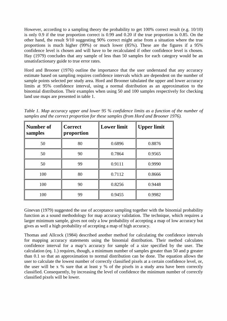
Hord and Brooner (1976) outline the importance that the user understand that any accuracyestimate based on sampling requires confidence intervals which are dependent on the number ofsample points selected per study area. Hord and Brooner tabulated the upper and lower accuracylimits at 95% confidence interval, using a normal distribution as an approximation to thebinomial distribution. Their examples when using 50 and 100 samples respectively for checkingland use maps are presented in table 1.

Table 1. Map accuracy upper and lower 95 % confidence limits as a function of the number ofsamples and the correct proportion for these samples (from Hord and Brooner 1976).

Number ofsamples

Correctproportion

Lower limit Upper limit

50 80 0.6896 0.8876

50 90 0.7864 0.9565

50 99 0.9111 0.9990

100 80 0.7112 0.8666

100 90 0.8256 0.9448

100 99 0.9455 0.9982

Ginevan (1979) suggested the use of acceptance sampling together with the binomial probabilityfunction as a sound methodology for map accuracy validation. The technique, which requires alarger minimum sample, gives not only a low probability of accepting a map of low accuracy butgives as well a high probability of accepting a map of high accuracy.

Thomas and Allcock (1984) described another method for calculating the confidence intervalsfor mapping accuracy statements using the binomial distribution. Their method calculatesconfidence interval for a map’s accuracy for sample of a size specified by the user. Thecalculation (eq. 1.) requires, though, a minimum number of samples greater than 50 and p greaterthan 0.1 so that an approximation to normal distribution can be done. The equation allows theuser to calculate the lowest number of correctly classified pixels at a certain confidence level, or,the user will be x % sure that at least y % of the pixels in a study area have been correctlyclassified. Consequently, by increasing the level of confidence the minimum number of correctlyclassified pixels will be lower.

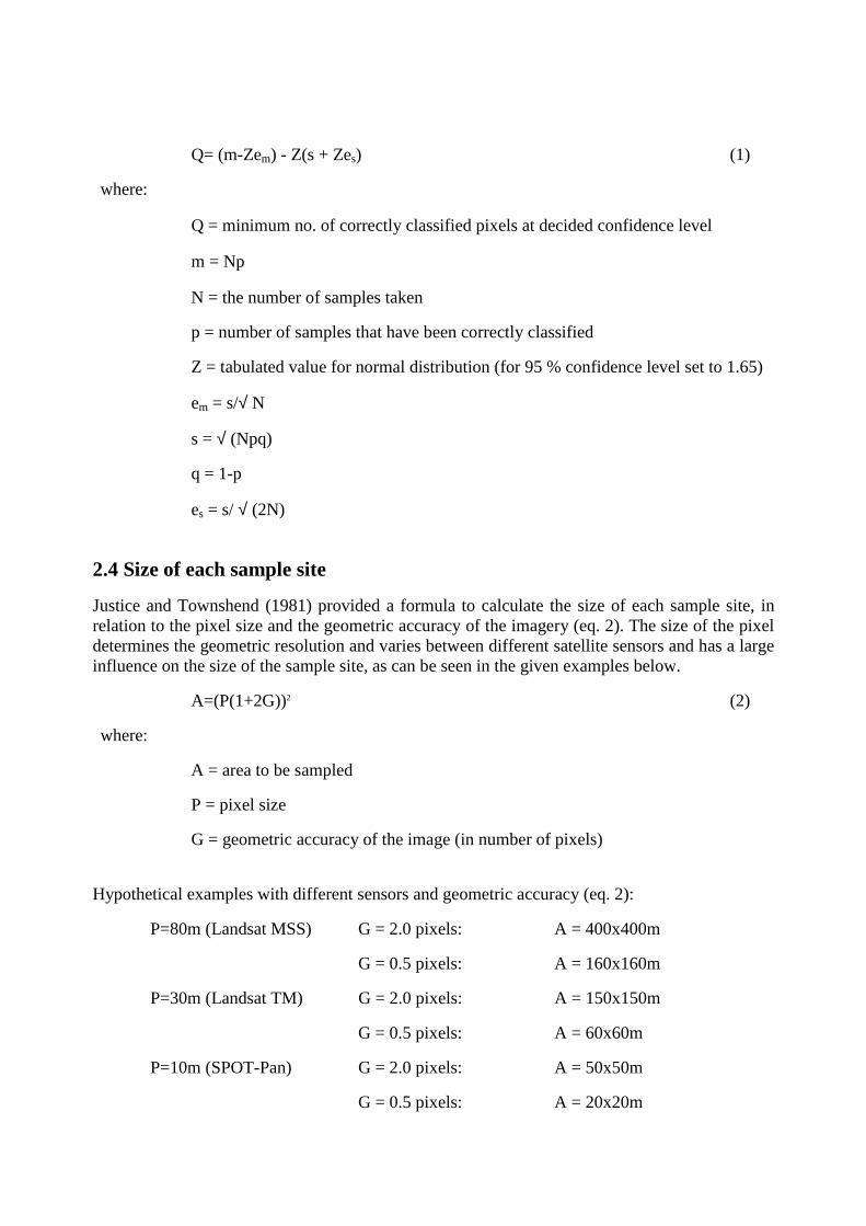
Q= (m-Zem) - Z(s + Zes) (1)

where:

Q = minimum no. of correctly classified pixels at decided confidence level

m = Np

N = the number of samples taken

p = number of samples that have been correctly classified

Z = tabulated value for normal distribution (for 95 % confidence level set to 1.65)

em = s/√ N

s =√ (Npq)

q = 1-p

es = s/√ (2N)

2.4 Size of each sample site

Justice and Townshend (1981) provided a formula to calculate the size of each sample site, inrelation to the pixel size and the geometric accuracy of the imagery (eq. 2). The size of the pixeldetermines the geometric resolution and varies between different satellite sensors and has a largeinfluence on the size of the sample site, as can be seen in the given examples below.

A=(P(1+2G))2 (2)

where:

A = area to be sampled

P = pixel size

G = geometric accuracy of the image (in number of pixels)

Hypothetical examples with different sensors and geometric accuracy (eq. 2):

P=80m (Landsat MSS) G = 2.0 pixels: A = 400x400m

G = 0.5 pixels: A = 160x160m

P=30m (Landsat TM) G = 2.0 pixels: A = 150x150m

G = 0.5 pixels: A = 60x60m

P=10m (SPOT-Pan) G = 2.0 pixels: A = 50x50m

G = 0.5 pixels: A = 20x20m

2.5 Number of subplots within one sample site

The number of subplots per sample site is mainly dependent upon the area to be sampled and itsspatial variability. In order to determine the spatial variability of a sample site, the standarddeviation of a number of spatially random measurements may be used to calculate therelationship between accuracy and number of samples (eq. 3) (Rao and Ulaby 1977). Therequired degree of accuracy (± a) should be set according to the study, quality of the remotelysensed data, etc.

Ns = (σ st/a)2 (3)

where:

Ns = number of subplots

σ s= standard deviation of measured values

t = tabulated student's t (n-1)

a = required degree of accuracy in units from true population mean

The calculation assumes that the data are normally distributed, and that the sample size used forextraction of the t-value (Student's t) in a pilot study (see example in section 3.3) is in the samerange as the sample calculated number of subplots. Degrees of freedom for the t-value arecalculated from (n - 1) where n is the number of samples used in the pilot study.

Hypothetical examples with different required accuracy (eq. 3):

t (n=10) = 2.3 σ s= 0.19 a=10 Ns = 19

t (n=10) = 2.3 σ s= 0.19 a=20 Ns = 5

From the above examples it is obvious that the number of subplots may vary considerably withthe level of required accuracy.

2.6 Size of subplots within one sample site

The size of the subplot should be chosen according to the nature of the studied parameter and theapplied sampling technique. If the studied parameter is highly variable, the subplot could bemade smaller and then a larger number will be required. If, however, the parameter is morehomogeneous fewer but larger subplots will be more efficient. The applied sampling techniquemay decide the size of the subplot.

The main considerations of the above review (section 2.3-2.6) on sampling designs for remotesensing applications are summarized in the following flow scheme (Figure 2).

Figure 2. Flow scheme for the collection of ground data. Boxes illustrate the main considerationsteps when designing a sampling scheme.

3. Vegetation cover data as an example of ground datacollection

3.1 Relationship between vegetation and remote sensing data

In rangeland management and land degradation studies, image processing of satellite data maypotentially provide quantitative data on vegetation cover and related parameters, e.g. wet and drybiomass. The various methods for estimating vegetation cover were already outlined in some ofthe early ecological publications dealing with vegetation cover (Arrhenius 1921, 1923). The mostcommon sampling techniques include visual estimation, quadrants, line intercept and point-centered quadrate (Küchler and Zonneveld 1988).

3.2 Case study

To illustrate the proposed sampling scheme and compare different ground cover estimationtechniques a field study was performed in a semi arid rangeland environment located near SidiBouZid in central Tunisia, North Africa (E 35° 00', N 9° 30'). Four sites with sparse vegetation,dominated by small bushes, perennial herbs and grasses were used. These sites are representativefor the variety of rangeland in the area (Figure 3). A scenario of Landsat TM data with thegeometric correction of 0.5 pixels was chosen as an example, which gave a sample site size of3600m2 or 60x60m (eq. 2). To compare the site level data with the data from subplot level, thesubplot level data were aggregated into the site level by averaging the subplots of each site.Different ground cover estimation techniques were tested: visual estimations both on site andsubplot levels, a line intercept, a quadrant and image analysis of ground photographs.

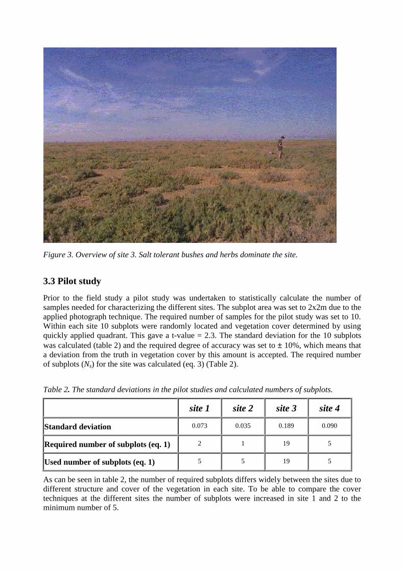
Figure 3. Overview of site 3. Salt tolerant bushes and herbs dominate the site.

3.3 Pilot study

Prior to the field study a pilot study was undertaken to statistically calculate the number ofsamples needed for characterizing the different sites. The subplot area was set to 2x2m due to theapplied photograph technique. The required number of samples for the pilot study was set to 10.Within each site 10 subplots were randomly located and vegetation cover determined by usingquickly applied quadrant. This gave a t-value = 2.3. The standard deviation for the 10 subplotswas calculated (table 2) and the required degree of accuracy was set to± 10%, which means thata deviation from the truth in vegetation cover by this amount is accepted. The required numberof subplots (Ns) for the site was calculated (eq. 3) (Table 2).

Table 2. The standard deviations in the pilot studies and calculated numbers of subplots.

site 1 site 2 site 3 site 4

Standard deviation 0.073 0.035 0.189 0.090

Required number of subplots (eq. 1) 2 1 19 5

Used number of subplots (eq. 1) 5 5 19 5

As can be seen in table 2, the number of required subplots differs widely between the sites due todifferent structure and cover of the vegetation in each site. To be able to compare the covertechniques at the different sites the number of subplots were increased in site 1 and 2 to theminimum number of 5.

3.4 Applied vegetation cover techniques

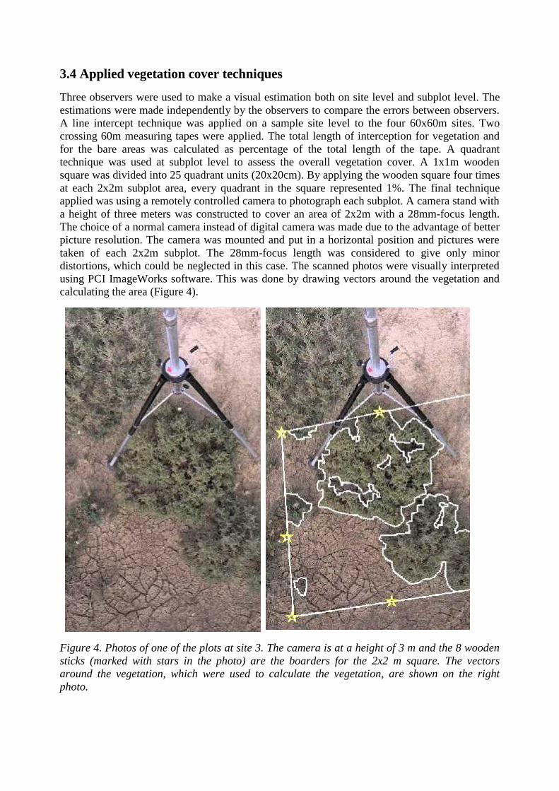
Three observers were used to make a visual estimation both on site level and subplot level. Theestimations were made independently by the observers to compare the errors between observers.A line intercept technique was applied on a sample site level to the four 60x60m sites. Twocrossing 60m measuring tapes were applied. The total length of interception for vegetation andfor the bare areas was calculated as percentage of the total length of the tape. A quadranttechnique was used at subplot level to assess the overall vegetation cover. A 1x1m woodensquare was divided into 25 quadrant units (20x20cm). By applying the wooden square four timesat each 2x2m subplot area, every quadrant in the square represented 1%. The final techniqueapplied was using a remotely controlled camera to photograph each subplot. A camera stand witha height of three meters was constructed to cover an area of 2x2m with a 28mm-focus length.The choice of a normal camera instead of digital camera was made due to the advantage of betterpicture resolution. The camera was mounted and put in a horizontal position and pictures weretaken of each 2x2m subplot. The 28mm-focus length was considered to give only minordistortions, which could be neglected in this case. The scanned photos were visually interpretedusing PCI ImageWorks software. This was done by drawing vectors around the vegetation andcalculating the area (Figure 4).

Figure 4. Photos of one of the plots at site 3. The camera is at a height of 3 m and the 8 woodensticks (marked with stars in the photo) are the boarders for the 2x2 m square. The vectorsaround the vegetation, which were used to calculate the vegetation, are shown on the rightphoto.

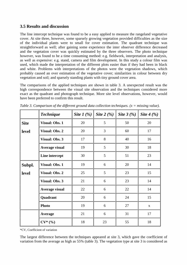
3.5 Results and discussion

The line intercept technique was found to be a easy applied to measure the rangeland vegetativecover. At site three, however, some sparsely growing vegetation provided difficulties as the sizeof the individual plants were to small for cover estimation. The quadrant technique wasstraightforward as well; after gaining some experience the inter observer difference decreasedand the vegetation cover was quickly estimated by the three observers. The photo techniquehowever, was found to be a time consuming method: e.g. fieldwork, interpretation and analysis,as well as expensive: e.g. stand, camera and film development. In this study a colour film wasused, which made the interpretation of the different plots easier than if they had been in blackand white. Problems with interpretations of the photos were the vegetation shadows, whichprobably caused an over estimation of the vegetative cover; similarities in colour between dryvegetation and soil; and sparsely standing plants with tiny ground cover area.

The comparisons of the applied techniques are shown in table 3. A unexpected result was thehigh correspondence between the visual site observation and the techniques considered moreexact as the quadrant and photograph technique. More site level observations, however, wouldhave been preferred to confirm this result.

Table 3. Comparison of the different ground data collection techniques. (x = missing value).

Technique Site 1 (%) Site 2 (%) Site 3 (%) Site 4 (%)

Visual: Obs. 1 20 5 50 20

Visual: Obs. 2 20 3 60 17

Visual: Obs. 3 17 8 40 16

Average visual 19 5 30 18

Site

level

Line intercept 30 5 51 23

Visual: Obs. 1 19 6 20 14

Visual: Obs. 2 25 5 23 15

Visual: Obs. 3 21 6 23 14

Average visual 22 6 22 14

Quadrant 20 6 24 15

Subpl.

level

Photo 19 6 27 x

Average 21 6 31 17

CV* (%) 18 23 55 18

*CV, Coefficient of variation

The largest difference between the techniques appeared at site 3, which gave the coefficient ofvariation from the average as high as 55% (table 3). The vegetation type at site 3 is considered as

the main factor for the large differences between its site and subplot levels. Higher values of theline intercept method at site 1 and 4 are more difficult to explain. The problem of dataaggregation from subplot to site level was also found by Zhou and Pilesjö (1996).

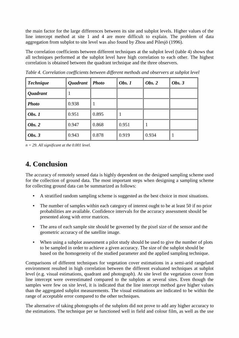
The correlation coefficients between different techniques at the subplot level (table 4) shows thatall techniques performed at the subplot level have high correlation to each other. The highestcorrelation is obtained between the quadrant technique and the three observers.

Table 4. Correlation coefficients between different methods and observers at subplot level

Technique Quadrant Photo Obs. 1 Obs. 2 Obs. 3

Quadrant 1

Photo 0.938 1

Obs. 1 0.951 0.895 1

Obs. 2 0.947 0.868 0.951 1

Obs. 3 0.943 0.878 0.919 0.934 1

n = 29. All significant at the 0.001 level.

4. ConclusionThe accuracy of remotely sensed data is highly dependent on the designed sampling scheme usedfor the collection of ground data. The most important steps when designing a sampling schemefor collecting ground data can be summarized as follows:

• A stratified random sampling scheme is suggested as the best choice in most situations.

• The number of samples within each category of interest ought to be at least 50 if no priorprobabilities are available. Confidence intervals for the accuracy assessment should bepresented along with error matrices.

• The area of each sample site should be governed by the pixel size of the sensor and thegeometric accuracy of the satellite image.

• When using a subplot assessment a pilot study should be used to give the number of plotsto be sampled in order to achieve a given accuracy. The size of the subplot should bebased on the homogeneity of the studied parameter and the applied sampling technique.

Comparisons of different techniques for vegetation cover estimations in a semi-arid rangelandenvironment resulted in high correlation between the different evaluated techniques at subplotlevel (e.g. visual estimations, quadrant and photograph). At site level the vegetation cover fromline intercept were overestimated compared to the subplots at several sites. Even though thesamples were few on site level, it is indicated that the line intercept method gave higher valuesthan the aggregated subplot measurements. The visual estimations are indicated to be within therange of acceptable error compared to the other techniques.

The alternative of taking photographs of the subplots did not prove to add any higher accuracy tothe estimations. The technique per se functioned well in field and colour film, as well as the use

of a digital photo-CD, proved to be a good choice. However, the photograph technique is timeconsuming, expensive and the equipment is sensitive and heavy to carry around. As theinterpretation of the photos involved some difficulties, using a quadrant is indicated to be boththe easiest and most accurate method in the studied type of environment.

When collecting vegetation cover data it is recommended to combine the quadrant method (pilotstudy) and visual method in carefully outlined sites. When skills of the fieldworkers haveincreased through using the quadrant the visual method can be used if the type of vegetation isfamiliar and the whole site is taken into consideration. If several field workers are involved theirconcordance ought to be checked regularly. If this can not be done or if the field workers areinexperienced the need for a more subjective method increases and the photographs of thesubplot should be considered. The study indicates that traditional methods of ground datacollection for remote sensing applications do not have to result in "ground lies". Determinationof a reliable and appropriate sampling scheme for the ground data collection should, however, begiven more attention when assuring accurate results in remote sensing studies.

5. AcknowledgementsWe would like to gratefully acknowledge the enthusiastic field assistance and contribution ofJessica Hellberg. We would also like to acknowledge Dr. Petter Pilesjö and Dr. Peter Schlyter fortheir assistance and contributions to this work. Thanks are also due to Dr. Lars Eklundh foruseful comments made upon drafts of this paper.

6. ReferencesArrhenius, O., 1921. Species and area,Journal of Ecology, 9:95-99.

Arrhenius, O., 1923. Statistical investigations in the constitution of plant associations,Ecology,4: 68-73.

Atkinson, P.M., 1991. Optimal ground-based sampling for remote sensing investigations:estimating the regional mean,Int. J. Remote Sensing,12, 559-567.

Atkinson, P.M., 1996. Optimal sampling strategies for raster-based geographical informationsystems,Global Ecology and Biogeography Letters, 5, 271-280.

Berry, B. L., and Baker, A.M., 1968. Geographic sampling,Spatial analysis, (Berry, B.L. andMarbles, D.F., editors), Prentice-Hall, Eaglewood Cliffs.

Clark W.V., and Hosking P.L., 1986.Statistical methods for geographer,John Wiley & Sons,New York.

Cochran W.G., 1977.Sampling techniques.John Wiley & Sons, New York.

Congalton, R.G., 1988a. A comparison of sampling schemes used in generating error matricesfor assessing the accuracy of maps generated from remotely sensed data,PhotogrammetricEngineering and Remote Sensing,54:593-600.

Congalton, R.G., 1988b.Using spatial autocorrelation analysis to explore the errors in mapsgenerated from remotely sensed data,Photogrammetric Engineering and Remote Sensing,54:587-592.

Congalton, R.G., 1991. A review of assessing the accuracy of classifications of remotely senseddata,Remote Sensing of Environment, 37: 35-46.

Curran, P.J., and Williamson, H.D., 1985. The accuracy of ground data used in remote sensinginvestigations,Int. J. Remote Sensing, 6:1637-1651.

Curran, P.J., and Williamson, H.D., 1986. Sample size for ground and remotely sensed data,Remote Sensing of Environment, 20:31-41.

Fitzpatrick-Lins, K., 1981: Comparison of sampling procedures and data analysis for a land-use and land-cover map,Photogrammetric Engineering and Remote Sensing,47:343-351.

Ginevan, M.E., 1979. Testing land-use map accuracy: another look,PhotogrammetricEngineering and Remote Sensing,45:1371-1377.

Hatfield, J.L., Kanemasu, E.T., Asrar, G., Jackson, R.D., Pinter, P.J., Reginato, R.J. and Idso,S.B., 1985. Leaf area estimates from spectral measurements over various planting dates of wheat.Int. J. Remote Sensing.6:167-175.

Hay, A.M., 1979. Sampling designs to test land-use map accuracy, PhotogrammetricEngineering and Remote Sensing,45:529-533.

Helldén U., 1980. A test of Landsat-2 imagery and digital data for thematic mapping, illustratedby an environmental study in northern Kenya. Lunds Universitets Naturgeografiska Institution.Rapporter och Notiser No 47.

Hord, M.R., and Brooner, W., 1976. Land-use map accuracy criteria.PhotogrammetricEngineering and Remote Sensing,42:671-677.

Justice, C.O., and Townshend, J. G., 1981. Integrating ground data with remote sensing.Terrainanalysis and remote sensing, (Townshend J.G., editor) George Allen and Uniwin, London.

Kuchler, A.W., and Zonneveld, I.S., 1988. Floristic analysis of vegetation,Handbook ofvegetation Science No 10 Vegetation mapping. (Leth.H., editor), Kluwer Academic Publishers,Dordrecht.

Lunetta, Ross S., Congalton, Russell G., Lynn, Fenstermaker K., Jensen John R., McGwireKenneth C. and Tinney Larry R. 1991. Remote sensing and geographic information systems dataintegration: Error sources and research issues.Photogrammetric Engineering and RemoteSensing,57:677-687.

Rao, R. S., and Ulaby, F.T., 1977. Optimal sampling techniques for ground truth data inmicrowave remote sensing of soil moisture.Remote Sensing of Environment, 6:289-301.

Richard, J.A., 1993.Remote sensing digital image analysis. Springer Verlag, Berlin.

Rosenfield, G.H., Fitzpatrick-Lins, K., and Ling H. 1982. Sampling for thematic map accuracytesting.Photogrammetric Engineering and Remote Sensing,48:131-137.

Swain, P.H., and Davis, S.M., 1978.Remote sensing: The quantitative approach.McGraw-Hill,New York.

Thomas, I.L., and Allcock, G.McK., 1984. Determining the confidence level for a classification.Photogrammetric Engineering and Remote Sensing,50:14911496.

Van Genderen, J.L., and Lock, B.F. 1977. Testing land use map accuracy.Photogrammetric

Engineering and Remote Sensing,43:1135-1137.

Van Genderen, J.L., Lock, B.F., and Vass, P.A., 1978. Remote sensing: statistical testing ofthematic map accuracy.Remote Sensing of Environment, 7:3-14.

Zhou, Q., and Pilesjö, P., 1996, Improving ground truthing for integrating remotely sensed dataand GIS.International Society for Photogrammetry and Remote Sensing. Workshop on NewDevelopments in Geographical Information Systems, (Milan, Italy, 6-8 March 1996).