Gröbner Bases - Quick Updates and Extended Snapshotsdacox.people.amherst.edu/lectures/EACA.pdf ·...
122
Gröbner Bases Quick Updates and Extended Snapshots David A. Cox Department of Mathematics and Computer Science Amherst College [email protected] EACA 2012, Alcalá David A. Cox (Amherst College) Gröbner Bases EACA 2012, Alcalá 1 / 42
Transcript of Gröbner Bases - Quick Updates and Extended Snapshotsdacox.people.amherst.edu/lectures/EACA.pdf ·...

Gröbner BasesQuick Updates and Extended Snapshots
David A. Cox
Department of Mathematics and Computer ScienceAmherst College
EACA 2012, Alcalá
David A. Cox (Amherst College) Gröbner Bases EACA 2012, Alcalá 1 / 42

Outline
Four Quick Updates:
The F5 Algorithm
One-Point Algebraic Geometry Codes
Cost Minimization of Series-Parallel System
May 2012
Four Extended Snapshots:
Graph Colorings
The Join-Meet Ideal of a Finite Lattice
The Nullstellensatz
Geometric Theorem Discovery
David A. Cox (Amherst College) Gröbner Bases EACA 2012, Alcalá 2 / 42

Update #1: The F5 Algorithm
In 2002, Faugére proposed his F5 algorithm for computing Gröbnerbases. Its termination was proved just recently!
S. Pan, Y. Hu and B. Wang, The Termination of Algorithms forComputing Gröbner Bases, arXiv:math.AC/1202.3524.
The F5 algorithm is generally believed as one of the fastest algorithmsfor computing Gröbner bases. However, its termination problem is stillunclear. Recently, an algorithm GVW and its variant GVWHS havebeen proposed, and their efficiency are comparable to the F5algorithm. . . . Taking into account this situation, we prove thetermination and correctness of the F5B algorithm. And we notice thatthe original F5 algorithm slightly differs from the F5B algorithm in theinsertion strategy on which the F5-rewritten criterion is based. . . .Therefore, we have a positive answer to the long standing problem ofproving the termination of the original F5 algorithm.
David A. Cox (Amherst College) Gröbner Bases EACA 2012, Alcalá 3 / 42

Update #1, Continued
V. Galkin, Termination of Original F5, arXiv:math.AC/1203.2402.
The original F5 algorithm described in Faugére’s paper is formulatedfor any homogeneous polynomial set input. The correctness of outputis shown for any input that terminates the algorithm, but the terminationitself is proved only for the case of input being regular polynomialsequence. This article shows that algorithm correctly terminates forany homogeneous input without any reference to regularity.
C. Eder, Sweetening the sour taste of inhomogeneous signature-basedGroebner basis computations, arXiv:math.AC/1203.6186.
In this paper we want to give an insight into the rather unknownbehaviour of signature-based Groebner basis algorithms, like F5,G2V, or GVW, for inhomogeneous input.
David A. Cox (Amherst College) Gröbner Bases EACA 2012, Alcalá 4 / 42

Update #2: One-Point Algebraic Geometry Codes
O. Geil, R. Matsumoto and D. Ruano, List decoding algorithmsbased on Gröbner bases for general one-point AG codes,arXiv:cs.IT/1201.6248.
We generalize the list decoding algorithm for Hermitian codesproposed by Lee and O’Sullivan based on Gröbner bases to generalone-point AG codes, under an assumption weaker than one used byBeelen and Brander. By using the same principle, we also generalizethe unique decoding algorithm for one-point AG codes over theMiura-Kamiya Cab curves proposed by Lee, Bras-Amorós andO’Sullivan to general one-point AG codes, without any assumption.
David A. Cox (Amherst College) Gröbner Bases EACA 2012, Alcalá 5 / 42

Update #3: Cost Minimization
F. Castro, J. Gago, I. Hartillo, J. Puerto and J. M. Ucha, Exact costminimization of a series-parallel system, arXiv:math.OC/1203.3307.
The redundancy allocation problem is formulated minimizing thedesign cost for a series-parallel system with multiple componentchoices whereas ensuring a given system reliability level. Theobtained model is a nonlinear integer programming problem with a nonlinear, non separable constraint. We propose an algebraic method,based on Gröbner bases, to obtain the exact solution of the problem.In addition, we provide a closed form for the required Gröbner bases,avoiding the bottleneck associated with the computation, andpromising computational results.
David A. Cox (Amherst College) Gröbner Bases EACA 2012, Alcalá 6 / 42

Update #4: May 2012
D. R. Grayson, A. Seceleanu and M. E. Stillman, Computations in intersectionrings of flag bundles, arXiv:math.AG/1205.4190.
Intersection rings of flag varieties are generated by Chern classes of thetautological bundles modulo relations coming from multiplicativity of totalChern classes. We describe the Groebner bases of the ideals of relations.
V. Galkin, Simple signature-based Groebner basis algorithm,arXiv:math.AC/1205.6050
This paper presents an algorithm for computing Groebner bases based uponlabeled polynomials and ideas from the algorithm F5.
D. J. Wilson, R. J. Bradford and J. H. Davenport, Speeding up CylindricalAlgebraic Decomposition by Gröbner bases, arXiv:cs.SC/1205.6285.
Gröbner Bases and Cylindrical Algebraic Decomposition are generallythought of as two, rather different, methods of looking at systems of equationsand, in the case of Cylindrical Algebraic Decomposition, inequalities.
David A. Cox (Amherst College) Gröbner Bases EACA 2012, Alcalá 7 / 42

Update Summary
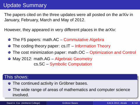
The papers cited on the three updates were all posted on the arXiv inJanuary, February, March and May of 2012.
However, they appeared in very different places in the arXiv:
The F5 papers: math.AC – Commutative Algebra
The coding theory paper: cs.IT – Information Theory
The cost minimization paper: math.OC – Optimization and Control
May 2012: math.AG – Algebraic Geometrycs.SC – Symbolic Computation
This shows:The continued activity in Gröbner bases.
The wide range of areas of mathematics and computer scienceinvolved.
David A. Cox (Amherst College) Gröbner Bases EACA 2012, Alcalá 8 / 42

Update Summary
The papers cited on the three updates were all posted on the arXiv inJanuary, February, March and May of 2012.
However, they appeared in very different places in the arXiv:
The F5 papers: math.AC – Commutative Algebra
The coding theory paper: cs.IT – Information Theory
The cost minimization paper: math.OC – Optimization and Control
May 2012: math.AG – Algebraic Geometrycs.SC – Symbolic Computation
This shows:The continued activity in Gröbner bases.
The wide range of areas of mathematics and computer scienceinvolved.
David A. Cox (Amherst College) Gröbner Bases EACA 2012, Alcalá 8 / 42

Snapshot #1: Graph Colorings
Let G = (V ,E) be a graph with vertices V = {1, . . . ,n}.
DefinitionA k-coloring of G is a function from V to a set of k colors such thatadjacent vertices have distinct colors.
Example
vertices = 81 squaresedges = links between:• squares in same column• squares in same row• squares in same 3× 3
Colors = {1,2, . . . ,9}
Goal: Extend the partialcoloring to a full coloring.
3 5
1 2 9
2
3
9
5
8
7
4
6
13
4
3
3
2
6
7 6
5
4
1
David A. Cox (Amherst College) Gröbner Bases EACA 2012, Alcalá 9 / 42

Graph Ideal
DefinitionThe k-coloring ideal of G is the ideal IG,k ⊆ C[xi | i ∈ V ] generated by:
for all i ∈ V : xki − 1
for all ij ∈ E : xk−1i + xk−2
i xj + · · ·+ xixk−2j + xk−1
j .
LemmaV(IG,k ) ⊆ Cn consists of all k-colorings of G for the set of colorsconsisting of the k th roots of unity
µn = {1, ζk , ζ2k , . . . , ζ
k−1k }, ζk = e2πi/k .
Proof.(xk
i − 1)− (xkj − 1)
xi − xj= xk−1
i + xk−2i xj + · · ·+ xk−1
j .
David A. Cox (Amherst College) Gröbner Bases EACA 2012, Alcalá 10 / 42

The Existence of Colorings
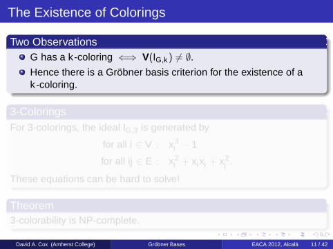
Two ObservationsG has a k-coloring ⇐⇒ V(IG,k ) 6= ∅.
Hence there is a Gröbner basis criterion for the existence of ak-coloring.
3-ColoringsFor 3-colorings, the ideal IG,3 is generated by
for all i ∈ V : x3i − 1
for all ij ∈ E : x2i + xixj + x2
j .
These equations can be hard to solve!
Theorem3-colorability is NP-complete.
David A. Cox (Amherst College) Gröbner Bases EACA 2012, Alcalá 11 / 42

The Existence of Colorings
Two ObservationsG has a k-coloring ⇐⇒ V(IG,k ) 6= ∅.
Hence there is a Gröbner basis criterion for the existence of ak-coloring.
3-ColoringsFor 3-colorings, the ideal IG,3 is generated by
for all i ∈ V : x3i − 1
for all ij ∈ E : x2i + xixj + x2
j .
These equations can be hard to solve!
Theorem3-colorability is NP-complete.
David A. Cox (Amherst College) Gröbner Bases EACA 2012, Alcalá 11 / 42
Example
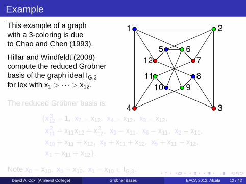
This example of a graphwith a 3-coloring is dueto Chao and Chen (1993).
Hillar and Windfeldt (2008)compute the reduced Gröbnerbasis of the graph ideal IG,3for lex with x1 > · · · > x12.
1 2
34
5 6
7
8
910
11
12
The reduced Gröbner basis is:
{x312 − 1, x7 − x12, x4 − x12, x3 − x12,
x211 + x11x12 + x2
12, x9 − x11, x6 − x11, x2 − x11,
x10 + x11 + x12, x8 + x11 + x12, x5 + x11 + x12,
x1 + x11 + x12}.
Note x8 − x10, x5 − x10, x1 − x10 ∈ IG,3.David A. Cox (Amherst College) Gröbner Bases EACA 2012, Alcalá 12 / 42

Example
This example of a graphwith a 3-coloring is dueto Chao and Chen (1993).
Hillar and Windfeldt (2008)compute the reduced Gröbnerbasis of the graph ideal IG,3for lex with x1 > · · · > x12.
1 2
34
5 6
7
8
910
11
12
The reduced Gröbner basis is:
{x312 − 1, x7 − x12, x4 − x12, x3 − x12,
x211 + x11x12 + x2
12, x9 − x11, x6 − x11, x2 − x11,
x10 + x11 + x12, x8 + x11 + x12, x5 + x11 + x12,
x1 + x11 + x12}.
Note x8 − x10, x5 − x10, x1 − x10 ∈ IG,3.David A. Cox (Amherst College) Gröbner Bases EACA 2012, Alcalá 12 / 42

Uniquely k -Colorable Graphs
The Chao/Chen graph has essentially only one 3-coloring.
DefinitionA graph G is uniquely k-colorable if it has a unique k-coloring up thepermutation of the colors.
Hillar and Windfeldt show that unique k-colorability is easy to detectusing Gröbner bases.
We start with a k-coloring of G that uses all k colors. Assume the kcolors occur among the last k vertices. Then:
Use variables x1, . . . , xn−k , y1, . . . , yk with lex order
x1 > · · · > xn−k > y1 > · · · > yk .
Use these variables to label the vertices of G.
David A. Cox (Amherst College) Gröbner Bases EACA 2012, Alcalá 13 / 42

Some Interesting Polynomials
Consider the following polynomials:
ykk − 1
hj(yj , . . . , yk ) =∑
αj+···+αk=j yαj
j · · · yαkk , j = 1, . . . , k − 1
xi − yj , color(xi) = color(yj), j ≥ 2
xi + y2 + · · ·+ yk , color(xi) = color(y1).
In this notation, the Gröbner basis given earlier is:
{y33 − 1,
h2(y2, y3) = y22 + y2y3 + y2
3 , h1(y1, y2, y3) = y1 + y2 + y3,
x7 − y3, x4 − y3, x3 − y3, x9 − y2, x6 − y2, x2 − y2,
x8 + y2 + y3, x5 + y2 + y3, x1 + y2 + y3}.
David A. Cox (Amherst College) Gröbner Bases EACA 2012, Alcalá 14 / 42

A Theorem
Summary:
G has vertices x1, . . . , xn−k , y1, . . . , yk .
G has a k-coloring where y1, . . . , yk get all the colors.
C[x,y] has lex with x1 > · · · > xn−k > y1 > · · · > yk .
Using this data, we create:
The coloring ideal IG,k ⊆ C[x,y].
The n polynomials g1, . . . ,gn given byyk
k − 1, hj(yj , . . . , yk ), xi − yj , xi + y2 + · · ·+ yk ,
Theorem (Hillar and Windfeldt)The following are equivalent:
G is uniquely k-colorable.
g1, . . . ,gn ∈ IG,k .
{g1, . . . ,gn} is the reduced Gröbner basis for IG,k .
David A. Cox (Amherst College) Gröbner Bases EACA 2012, Alcalá 15 / 42

A Final Amusement
To solve this sudoku, use:
• 81 variables xij , 1 ≤ i , j ≤ 9.• Relabel the 9 variables for
red squares as y1, . . . , y9.• The graph ideal IG,9.• The 9 polynomials y9
9 − 1,h8(y8, y9),h7(y7, y8, y9),h6(y6, y7, y8, y9), . . . ,h1(y1, . . . , y9) = y1 + · · ·+ y9.• The 16 polynomials x31 − y7,
x33 − y6, x37 − y2, . . .
3 5
1 2 9
8
7
4
6
2
3
9
5
13
4
3
3
2
6
7 6
5
4
1
Assuming a unique solution, the Gröbner basis of the ideal generatedby these polynomials will contain x11 − yi , etc. This will tell us how tofill in the blank squares!
David A. Cox (Amherst College) Gröbner Bases EACA 2012, Alcalá 16 / 42

Comments and References
This is a terrible way to solve a 9× 9 sudoku. Doug Leonard hasbeen able to implement this in Magma, but only by working overthe finite field F11 and limiting interreductions to generators ofdegree at most 4.
On the other hand, doing the 4× 4 sudoku this way makes anexcellent student project.
ReferenceC. Hillar, T. Windfeldt, Algebraic characterization of uniquelyvertex colorable graphs, J. Comb. Th., Ser. B 98 (2008), 400–414.
David A. Cox (Amherst College) Gröbner Bases EACA 2012, Alcalá 17 / 42

Snapshot #2: Join-Meet Ideals
Graphs are not the only combinatorial objects that give interestingideals. Here we explore ideals associated to finite lattices.
DefinitionA lattice is a partially ordered set L such that every a,b ∈ L have asup a ∨ b and an inf a ∧ b.
All lattices in this talk will be assumed to be finite.
DefinitionA lattice L is:
distributive if a ∧ (b ∨ c) = (a ∧ b) ∨ (a ∧ c) for all a,b, c ∈ L.
modular if a ≤ b implies a ∨ (c ∧ b) = (a ∨ c) ∧ b for all c ∈ L.
Every distributive lattice is modular; the converse is not true.
David A. Cox (Amherst College) Gröbner Bases EACA 2012, Alcalá 18 / 42

Join-Meet Ideals
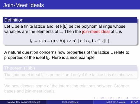
DefinitionLet L be a finite lattice and let k [L] be the polynomial rings whosevariables are the elements of L. Then the join-meet ideal of L is
IL = 〈a b − (a ∨ b)(a ∧ b) | a,b ∈ L〉 ⊆ k [L].
A natural question concerns how properties of the lattice L relate toproperties of the ideal IL. Here is a nice example.
Theorem (Hibi)The join-meet ideal IL is prime if and only if the lattice L is distributive.
We now discuss some of the interesting relations between Gröbnerbases and join-meet ideals.
David A. Cox (Amherst College) Gröbner Bases EACA 2012, Alcalá 19 / 42
Join-Meet Ideals
DefinitionLet L be a finite lattice and let k [L] be the polynomial rings whosevariables are the elements of L. Then the join-meet ideal of L is
IL = 〈a b − (a ∨ b)(a ∧ b) | a,b ∈ L〉 ⊆ k [L].
A natural question concerns how properties of the lattice L relate toproperties of the ideal IL. Here is a nice example.
Theorem (Hibi)The join-meet ideal IL is prime if and only if the lattice L is distributive.
We now discuss some of the interesting relations between Gröbnerbases and join-meet ideals.
David A. Cox (Amherst College) Gröbner Bases EACA 2012, Alcalá 19 / 42

Gröbner Bases and Distributive Lattices
We first give a Gröbner basis criterion for a lattice to be distributive.
TheoremLet L be a lattice. The following are equivalent:
1 L is distributive.2 IL is prime.3 {a b − (a ∨ b)(a ∧ b) | a,b ∈ L incomparable} is a
Gröbner basis for IL for any monomial order satisfyinga b > (a ∨ b)(a ∧ b) when a,b are incomparable.
(1)⇔ (2)⇒ (3) was proved by Hibi in 1987.
(3)⇒ (1) was noted by Qureshi in 2012.
David A. Cox (Amherst College) Gröbner Bases EACA 2012, Alcalá 20 / 42

Modular Non-Distributive Lattices
We next study IL for some modular non-distributive lattices L.Here, Gröbner bases play a key role in the proof.
We begin with two closely related lattices. The one on the left isdistributive; the one on the right is modular but not distributive.
x1
x2
xk
xk +1
xn -1
xn
y1
y2
yk
yk +1
yn -1
yn
x1
x2
xk
xk +1
xn -1
xn
y1
y2
yk
yk +1
yn -1
yn
z
The lattice on the right will be denoted Lk .
David A. Cox (Amherst College) Gröbner Bases EACA 2012, Alcalá 21 / 42

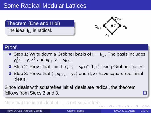
Some Radical Modular Lattices
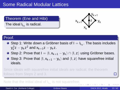
Theorem (Ene and Hibi)The ideal ILk
is radical.xk
xk +1yk
yk +1
z
Proof.Step 1: Write down a Gröbner basis of I = ILk
. The basis includesy2
k z − yk z2 and xk+1z − yk z.
Step 2: Prove that I = 〈I, xk+1 − yk 〉 ∩ 〈I, z〉 using Gröbner bases.
Step 3: Prove that 〈I, xk+1 − yk 〉 and 〈I, z〉 have squarefree initialideals.
Since ideals with squarefree initial ideals are radical, the theoremfollows from Steps 2 and 3.
Note that the initial ideal of ILkis not squarefree.
David A. Cox (Amherst College) Gröbner Bases EACA 2012, Alcalá 22 / 42

Some Radical Modular Lattices
Theorem (Ene and Hibi)The ideal ILk
is radical.xk
xk +1yk
yk +1
z
Proof.Step 1: Write down a Gröbner basis of I = ILk
. The basis includesy2
k z − yk z2 and xk+1z − yk z.
Step 2: Prove that I = 〈I, xk+1 − yk 〉 ∩ 〈I, z〉 using Gröbner bases.
Step 3: Prove that 〈I, xk+1 − yk 〉 and 〈I, z〉 have squarefree initialideals.
Since ideals with squarefree initial ideals are radical, the theoremfollows from Steps 2 and 3.
Note that the initial ideal of ILkis not squarefree.
David A. Cox (Amherst College) Gröbner Bases EACA 2012, Alcalá 22 / 42

References
ReferencesT. Hibi, Distributive lattices, affine semigroup rings and algebraswith straightening laws, in Commutative Algebra andCombinatorics (Kyoto, 1985), North-Holland, Amsterdam, 1987,93–109,
A. Qureshi, Indespensible Hibi relations and Gröbner bases,arXiv:math.CA/1203.0438.
V. Ene and T. Hibi, The join-meet ideal of a finite lattice,arXiv:math.AC/1203.6794.
David A. Cox (Amherst College) Gröbner Bases EACA 2012, Alcalá 23 / 42

Snapshot #3: The Nullstellensatz
There are many proofs of the Nullstellensatz. Here we present a proofdue to Lev Glebsky that uses Gröbner bases.
Notationk [u,x ], x = (x1, . . . , xn−1), is a polynomial ring in n variables.
a ∈ k gives the evaluation map eva : k [u,x ]→ k [x ] defined byeva(p) = p(a,x).
TheoremLet k be an algebraically closed field and let I ( k [u,x ] be an ideal.Then there is a ∈ k such that eva(I) ( k [x ].
Applying this theorem repeatedly, we can find a1, . . . ,an ∈ k witheva1,...,an(I) ( k , hence eva1,...,an(I) = {0}. It follows that V(I) 6= ∅. Thisin turn implies the Nullstellensatz.
David A. Cox (Amherst College) Gröbner Bases EACA 2012, Alcalá 24 / 42

Case I
Assume I ∩ k [u] = 〈p〉, p 6= 0. Then p is nonconstant since I is aproper ideal.
Write p =∏r
i=1(u − ai)mi . Then
I = 〈p〉+ I =⋂r
i=1
(
〈u − ai〉mi + I
)
,
so that 〈u − ai〉mi + I is proper for some index i .
Observe that
〈u − ai〉mi + I ⊆ 〈u − ai〉+ I ⊆
√
〈u − ai〉mi + I.
Hence 〈u − ai〉+ I is also a proper ideal.
It follows easily that evai (I) ( k [x ].
David A. Cox (Amherst College) Gröbner Bases EACA 2012, Alcalá 25 / 42

Case II
This is where we use Gröbner bases.
Assume I ∩ k [u] = {0}. This easily implies that
J := ideal of k(u)[x ] generated by I
is a proper ideal of k(u)[x ].
Let G be a reduced Gröbner basis of J. Elements of G arepolynomials in x with coefficients in k(u). Let h ∈ k [u] be theLCM of all denominators of the coefficients of elements of G.
Since k is infinite, we can pick a ∈ k such that h(a) 6= 0.
Let Ra = {f/g ∈ k(u) | f ,g ∈ k [u], g(a) 6= 0}. Then the evaluationmap eva : k [u,x ] = k [u][x ]→ k [x ] extends to an evaluation map
eva : Ra[x ] −→ k [x ]
David A. Cox (Amherst College) Gröbner Bases EACA 2012, Alcalá 26 / 42
Case II, Continued
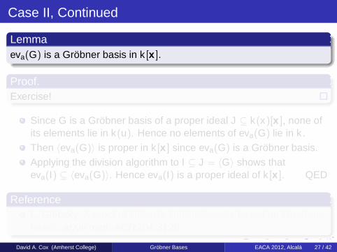
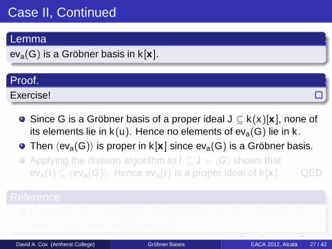
Lemmaeva(G) is a Gröbner basis in k [x ].
Proof.Exercise!
Since G is a Gröbner basis of a proper ideal J ⊆ k(x)[x ], none ofits elements lie in k(u). Hence no elements of eva(G) lie in k .Then 〈eva(G)〉 is proper in k [x ] since eva(G) is a Gröbner basis.Applying the division algorithm to I ⊆ J = 〈G〉 shows thateva(I) ⊆ 〈eva(G)〉. Hence eva(I) is a proper ideal of k [x ]. QED
ReferenceL. Glebsky, A proof of Hilbert’s Nullstellensatz based on Groebnerbases, arXiv:math.AC/1204.3128.
David A. Cox (Amherst College) Gröbner Bases EACA 2012, Alcalá 27 / 42

Case II, Continued
Lemmaeva(G) is a Gröbner basis in k [x ].
Proof.Exercise!
Since G is a Gröbner basis of a proper ideal J ⊆ k(x)[x ], none ofits elements lie in k(u). Hence no elements of eva(G) lie in k .Then 〈eva(G)〉 is proper in k [x ] since eva(G) is a Gröbner basis.Applying the division algorithm to I ⊆ J = 〈G〉 shows thateva(I) ⊆ 〈eva(G)〉. Hence eva(I) is a proper ideal of k [x ]. QED
ReferenceL. Glebsky, A proof of Hilbert’s Nullstellensatz based on Groebnerbases, arXiv:math.AC/1204.3128.
David A. Cox (Amherst College) Gröbner Bases EACA 2012, Alcalá 27 / 42

Snapshot #4: Geometric Theorem Discovery
Our final topic involves an application of comprehensive Gröbnersystems to the problem of discovering the correct hypotheses that givean interesting theorem in geometry.
Our discussion was inspired by a 2007 paper of Montes and Recio.
We begin with a 2006 example of Sato and Suzuki that illustratesspecialization of Gröbner bases.
David A. Cox (Amherst College) Gröbner Bases EACA 2012, Alcalá 28 / 42
Example 1
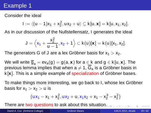
Consider the ideal
I := 〈(u − 1)x1 + x22 ,ux2 + u〉 ⊆ k [u,x ] = k [u, x1, x2].
As in our discussion of the Nullstellensatz, I generates the ideal
J =⟨
x1 +x2
2
u − 1, x2 + 1
⟩
⊂ k(u)[x ] = k(u)[x1, x2].
The generators G of J are a lex Gröbner basis for x1 > x2.
We will write ga = eva(g) = g(a,x) for a ∈ k and g ∈ k [u,x ]. Theprevious lemma implies that when a 6= 1, Ga is a Gröbner basis ink [x ]. This is a simple example of specialization of Gröbner bases.
To make things more interesting, we go back to I, whose lex Gröbnerbasis for x1 > x2 > u is
{ux1 − x1 + x22 ,ux2 + u, x1x2 + x1 − x3
2 − x22}
There are two questions to ask about this situation.David A. Cox (Amherst College) Gröbner Bases EACA 2012, Alcalá 29 / 42
First Question
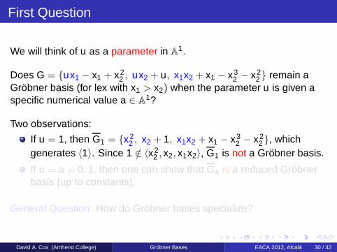
We will think of u as a parameter in A1.
Does G = {ux1 − x1 + x22 , ux2 + u, x1x2 + x1 − x3
2 − x22} remain a
Gröbner basis (for lex with x1 > x2) when the parameter u is given aspecific numerical value a ∈ A1?
Two observations:
If u = 1, then G1 = {x22 , x2 + 1, x1x2 + x1 − x3
2 − x22}, which
generates 〈1〉. Since 1 /∈ 〈x22 , x2, x1x2〉, G1 is not a Gröbner basis.
If u = a 6= 0,1, then one can show that Ga is a reduced Gröbnerbasis (up to constants).
General Question: How do Gröbner bases specialize?
David A. Cox (Amherst College) Gröbner Bases EACA 2012, Alcalá 30 / 42

First Question
We will think of u as a parameter in A1.
Does G = {ux1 − x1 + x22 , ux2 + u, x1x2 + x1 − x3
2 − x22} remain a
Gröbner basis (for lex with x1 > x2) when the parameter u is given aspecific numerical value a ∈ A1?
Two observations:
If u = 1, then G1 = {x22 , x2 + 1, x1x2 + x1 − x3
2 − x22}, which
generates 〈1〉. Since 1 /∈ 〈x22 , x2, x1x2〉, G1 is not a Gröbner basis.
If u = a 6= 0,1, then one can show that Ga is a reduced Gröbnerbasis (up to constants).
General Question: How do Gröbner bases specialize?
David A. Cox (Amherst College) Gröbner Bases EACA 2012, Alcalá 30 / 42

Second Question
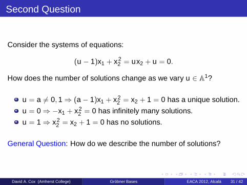
Consider the systems of equations:
(u − 1)x1 + x22 = ux2 + u = 0.
How does the number of solutions change as we vary u ∈ A1?
u = a 6= 0,1⇒ (a − 1)x1 + x22 = x2 + 1 = 0 has a unique solution.
u = 0⇒ −x1 + x22 = 0 has infinitely many solutions.
u = 1⇒ x22 = x2 + 1 = 0 has no solutions.
General Question: How do we describe the number of solutions?
David A. Cox (Amherst College) Gröbner Bases EACA 2012, Alcalá 31 / 42

Second Question
Consider the systems of equations:
(u − 1)x1 + x22 = ux2 + u = 0.
How does the number of solutions change as we vary u ∈ A1?
u = a 6= 0,1⇒ (a − 1)x1 + x22 = x2 + 1 = 0 has a unique solution.
u = 0⇒ −x1 + x22 = 0 has infinitely many solutions.
u = 1⇒ x22 = x2 + 1 = 0 has no solutions.
General Question: How do we describe the number of solutions?
David A. Cox (Amherst College) Gröbner Bases EACA 2012, Alcalá 31 / 42

Answers for the Example
Consider the following pairs:
(S1,G1) :=(
A1 \ {0,1}, {(u − 1)x1 + x22 ,ux2 + x}
)
(S2,G2) :=(
{0}, {x1 − x22}
)
(S3,G3) :=(
{1}, {1})
.
The Si are called segments. Note that:
Si is constructible, S1 ∪ S2 ∪ S3 = A1 is a partition.
For a ∈ Si , Gi a is a reduced Gröbner basis (up to constants).
For a ∈ Si , 〈LT(Gi a)〉 is independent of a.
〈LT(G1a)〉 = 〈x1, x2〉, 〈LT(G2a)〉 = 〈x1〉, 〈LT(G3a)〉 = 〈1〉 gives thenumber of solutions.
This is a minimal canonical comprehensive Gröbner system.
David A. Cox (Amherst College) Gröbner Bases EACA 2012, Alcalá 32 / 42

MCCGS
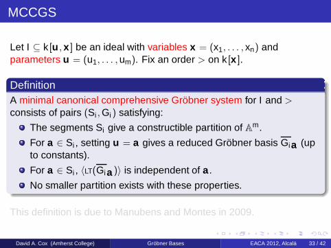
Let I ⊆ k [u ,x ] be an ideal with variables x = (x1, . . . , xn) andparameters u = (u1, . . . ,um). Fix an order > on k [x ].
DefinitionA minimal canonical comprehensive Gröbner system for I and >consists of pairs (Si ,Gi) satisfying:
The segments Si give a constructible partition of Am.
For a ∈ Si , setting u = a gives a reduced Gröbner basis Gia (upto constants).
For a ∈ Si , 〈LT(Gia )〉 is independent of a .
No smaller partition exists with these properties.
This definition is due to Manubens and Montes in 2009.
David A. Cox (Amherst College) Gröbner Bases EACA 2012, Alcalá 33 / 42

MCCGS
Let I ⊆ k [u ,x ] be an ideal with variables x = (x1, . . . , xn) andparameters u = (u1, . . . ,um). Fix an order > on k [x ].
DefinitionA minimal canonical comprehensive Gröbner system for I and >consists of pairs (Si ,Gi) satisfying:
The segments Si give a constructible partition of Am.
For a ∈ Si , setting u = a gives a reduced Gröbner basis Gia (upto constants).
For a ∈ Si , 〈LT(Gia )〉 is independent of a .
No smaller partition exists with these properties.
This definition is due to Manubens and Montes in 2009.
David A. Cox (Amherst College) Gröbner Bases EACA 2012, Alcalá 33 / 42

A False Theorem
Let CD be the diameter of acircle of radius 1. Fix A. Then:
• The line←→AE is tangent to the
circle at E .
• The lines←→AC and
←→ED meet at F .
False TheoremAE = AF .
Challenge: Discover reasonablehypotheses on A to make thetheorem true.
A
C DO
E
F
David A. Cox (Amherst College) Gröbner Bases EACA 2012, Alcalá 34 / 42
Hypotheses
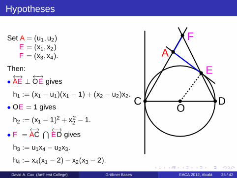
Set A = (u1,u2)E = (x1, x2)F = (x3, x4).
Then:
•←→AE ⊥
←→OE gives
h1 := (x1 − u1)(x1 − 1) + (x2 − u2)x2.
• OE = 1 gives
h2 := (x1 − 1)2 + x22 − 1.
• F =←→AC
⋂ ←→ED gives
h3 := u1x4 − u2x3.
h4 := x4(x1 − 2)− x2(x3 − 2).
A
C DO
E
F
David A. Cox (Amherst College) Gröbner Bases EACA 2012, Alcalá 35 / 42

More Hypotheses
We also need to assume:
• A 6= C, so
u1 6= 0 or u2 6= 0.
• E 6= D, so
x2 6= 2.
Conclusion: The ideal thatdescribes this problem is thesaturation
I := 〈h1,h2,h3,h4〉 : 〈(x2 − 2)u1, (x2 − 2)u2〉∞
in the ring k [u1,u2, x1, x2, x3, x4].
A
C DO
E
F
David A. Cox (Amherst College) Gröbner Bases EACA 2012, Alcalá 36 / 42

Strategy
Our false theorem asserts AE = AF . This gives
g := (u1 − x1)2 + (u2 − x2)
2 − (u1 − x3)2 − (u2 − x4)
2.
StrategyCompute a MCCGS for the ideal
I + 〈g〉 ⊆ k [u1,u2, x1, x2, x3, x4], u1,u2 parameters.
Intuition
The false theorem is true for those u = a ∈ A2 for which
∅ 6= V(Ia + 〈ga 〉) ⊆ A4.
David A. Cox (Amherst College) Gröbner Bases EACA 2012, Alcalá 37 / 42

The MCCGS
The MCCGS for I + 〈g〉 ⊆ k [u1,u2, x1, x2, x3, x4] under lex order withx1 > x2 > x3 > x4 is
(S1,G1) ∪ · · · ∪ (S6,G6)
The Si and Leading Terms
i Si LT(Gia )
1 A2 \(
V(u21 + u2
2 − 2u1) ∪ V(u1))
1
2 V(u21 + u2
2 − 2u1) \ {(0,0), (2,0)} x1, x2, x3, x24
3 V(u1) \ {(0,0), (0,±i)} x1, x2, x3, x24
4 {(0,±i)} x1, x2, x3, x4
5 {(2,0)} x1, x22 , x3, x2
4
6 {(0,0)} x1, x2, x23 , x
24
David A. Cox (Amherst College) Gröbner Bases EACA 2012, Alcalá 38 / 42

Consequences of the MCCGS
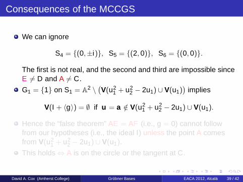
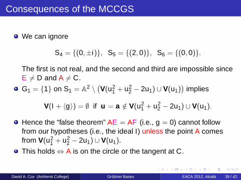
We can ignore
S4 = {(0,±i)}, S5 = {(2,0)}, S6 = {(0,0)}.
The first is not real, and the second and third are impossible sinceE 6= D and A 6= C.
G1 = {1} on S1 = A2 \(
V(u21 + u2
2 − 2u1) ∪ V(u1))
implies
V(I + 〈g〉) = ∅ if u = a /∈ V(u21 + u2
2 − 2u1) ∪ V(u1).
Hence the “false theorem” AE = AF (i.e., g = 0) cannot followfrom our hypotheses (i.e., the ideal I) unless the point A comesfrom V(u2
1 + u22 − 2u1) ∪ V(u1).
This holds⇔ A is on the circle or the tangent at C.
David A. Cox (Amherst College) Gröbner Bases EACA 2012, Alcalá 39 / 42
Consequences of the MCCGS
We can ignore
S4 = {(0,±i)}, S5 = {(2,0)}, S6 = {(0,0)}.
The first is not real, and the second and third are impossible sinceE 6= D and A 6= C.
G1 = {1} on S1 = A2 \(
V(u21 + u2
2 − 2u1) ∪ V(u1))
implies
V(I + 〈g〉) = ∅ if u = a /∈ V(u21 + u2
2 − 2u1) ∪ V(u1).
Hence the “false theorem” AE = AF (i.e., g = 0) cannot followfrom our hypotheses (i.e., the ideal I) unless the point A comesfrom V(u2
1 + u22 − 2u1) ∪ V(u1).
This holds⇔ A is on the circle or the tangent at C.
David A. Cox (Amherst College) Gröbner Bases EACA 2012, Alcalá 39 / 42

Conclusion
A
C DO
E
F In order for AE = AF , we must have
“A is on the circle or the tangent at C”
This is detected by the remainingsegments of the MCCGS:
A on the circle: S2 =V(u2
1 + u22 − 2u1) \ {(0,0), (2,0)}
A on the tangent: S3 =V(u1) \ {(0,0), (0,±i)}
A on the CircleAE = AF is true but boring.
David A. Cox (Amherst College) Gröbner Bases EACA 2012, Alcalá 40 / 42

Conclusion
A
C DO
E
F In order for AE = AF , we must have
“A is on the circle or the tangent at C”
This is detected by the remainingsegments of the MCCGS:
A on the circle: S2 =V(u2
1 + u22 − 2u1) \ {(0,0), (2,0)}
A on the tangent: S3 =V(u1) \ {(0,0), (0,±i)}
A on the CircleAE = AF is true but boring.
A = E = F
C DO
David A. Cox (Amherst College) Gröbner Bases EACA 2012, Alcalá 40 / 42

A on the Tangent
When A is on the tangent,we get the picture to the right.
There are two choices for E :
• For E1, we getF1 = E1, so AE = AFis true but boring.
• For E2, we get aninteresting theorem!
This is automatic theoremdiscovery using MCCGS.
A
C DO
E2
F2
F1 = E1 =
A
C DO
E
F
David A. Cox (Amherst College) Gröbner Bases EACA 2012, Alcalá 41 / 42

References
ReferencesM. Manubens, A. Montes, Minimal canonical comprehensive Groebnersystems, J. of Symbolic Comput. 44 (2009) 463–478.
A. Montes, T. Recio, Automatic discovery of geometric theorems usingminimal canonical comprehensive Groebner systems, In: AutomaticDeduction in Geometry, Proc. ADG 2006, Lect. Notes in AI 4869,Springer, 2007, pp. 113–138.
Recent DevelopmentA. Montes, M. Wibmer, Gröbner bases for polynomial systems withparameters, J. of Symbolic Comput. 45 (2010) 1391–1425.
Introduces Gröbner covers.
“Therefore the main focus of this article is not on the efficiency of thealgorithm but on computing a Gröbner system that has as few segmentsas possible and satisfies some additional nice properties.”
David A. Cox (Amherst College) Gröbner Bases EACA 2012, Alcalá 42 / 42


![Gröbner Bases Tutorial - David A. Coxdacox.people.amherst.edu/lectures/gb1.handout.pdfLet G be a Gröbner basis of I for a monomial order > that eliminates x. Then G∩k[y] is a Gröbner](https://static.fdocuments.net/doc/165x107/5ad6f0287f8b9a32618bad97/grbner-bases-tutorial-david-a-g-be-a-grbner-basis-of-i-for-a-monomial-order-that.jpg)