Thermodynamic Behaviorof particular f R,T Gravity Models ...

Gravity Models Elena Nikolaeva, Egon Elbre,
Roland Pihlakas
MTAT.03.251 Graph Mining

Introduction G=(V,C) network graph Origin Destination Flow as traffic
MTAT.03.251 Graph Mining
FLOW

Traffic flow
http://www.mundi.net/maps/maps_014/ MTAT.03.251 Graph Mining

Characteristics Of The Network Flows
MTAT.03.251 Graph Mining

Characteristics Of The Network Flows How does the traffic move throughout the network?
MTAT.03.251 Graph Mining

Characteristics Of The Network Flows How does the traffic move throughout the network?
Routing Matrix
MTAT.03.251 Graph Mining

Routing Matrix Captures the manner in which traffic moves throughout the
network.
B - binary values
- fraction of flow in case multiple routes are possible
MTAT.03.251 Graph Mining Figures are from Lauri Eskor’s slides
AC AD BD BC CD
1 1 0 0 0 0
2 0 1 1 1 0
3 0 1 1 0 1
Be;ij=
B
C D
A 1
2
3

Characteristics Of The Network Flows How much traffic flows from point A to point B?
MTAT.03.251 Graph Mining

Characteristics Of The Network Flows How much traffic flows from point A to point B?
Traffic Matrix
MTAT.03.251 Graph Mining

Constructing Traffic Matrix
Copyright © 1998-2011, Dr. Jean-Paul Rodrigue, Dept. of Global Studies & Geography, Hofstra University.
A B C D E Ti
A 0 0 50 0 0 50
B 0 0 60 0 30 90
C 0 0 0 30 0 30
D 20 0 80 0 20 120
E 0 0 90 10 0 100
Tj 20 0 280 40 50 390
A
C
B
E D
20
20
10
30
MTAT.03.251 Graph Mining

Origin-Destination Matrix (Traffic Matrix)
Where Zij is the total volume of traffic flowing from origin vertex i to a destination vertex j in a given period of time.
Net out-flow corresponding to vertices i
Net in-flow corresponding to vertices j
MTAT.03.251 Graph Mining

Link Totals
,where Xe – the total flow over a given link e∈ E
,where Z-traffic matrix written as a vector
MTAT.03.251 Graph Mining
AC AD BD BC CD
1 0 0 0 0
0 1 1 1 0
0 1 1 0 1 B
C D
A 1
2
3 X
ZAC
ZAD
ZBD
ZBC
ZCD
=
X1
X2
X3
X B Z
€
Xe = Be;ij × Ziji, j∑

Characteristics Of The Network Flows How much will it “cost” us?
MTAT.03.251 Graph Mining

Characteristics Of The Network Flows How much will it “cost” us?
Cost
MTAT.03.251 Graph Mining
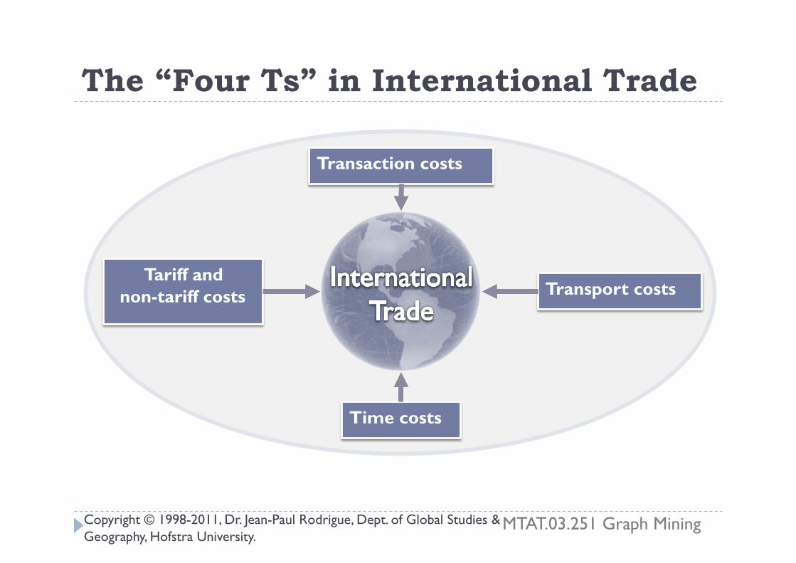
The “Four Ts” in International Trade
Copyright © 1998-2011, Dr. Jean-Paul Rodrigue, Dept. of Global Studies & Geography, Hofstra University.
Transaction costs
Tariff and non-tariff costs Transport costs
Time costs
MTAT.03.251 Graph Mining
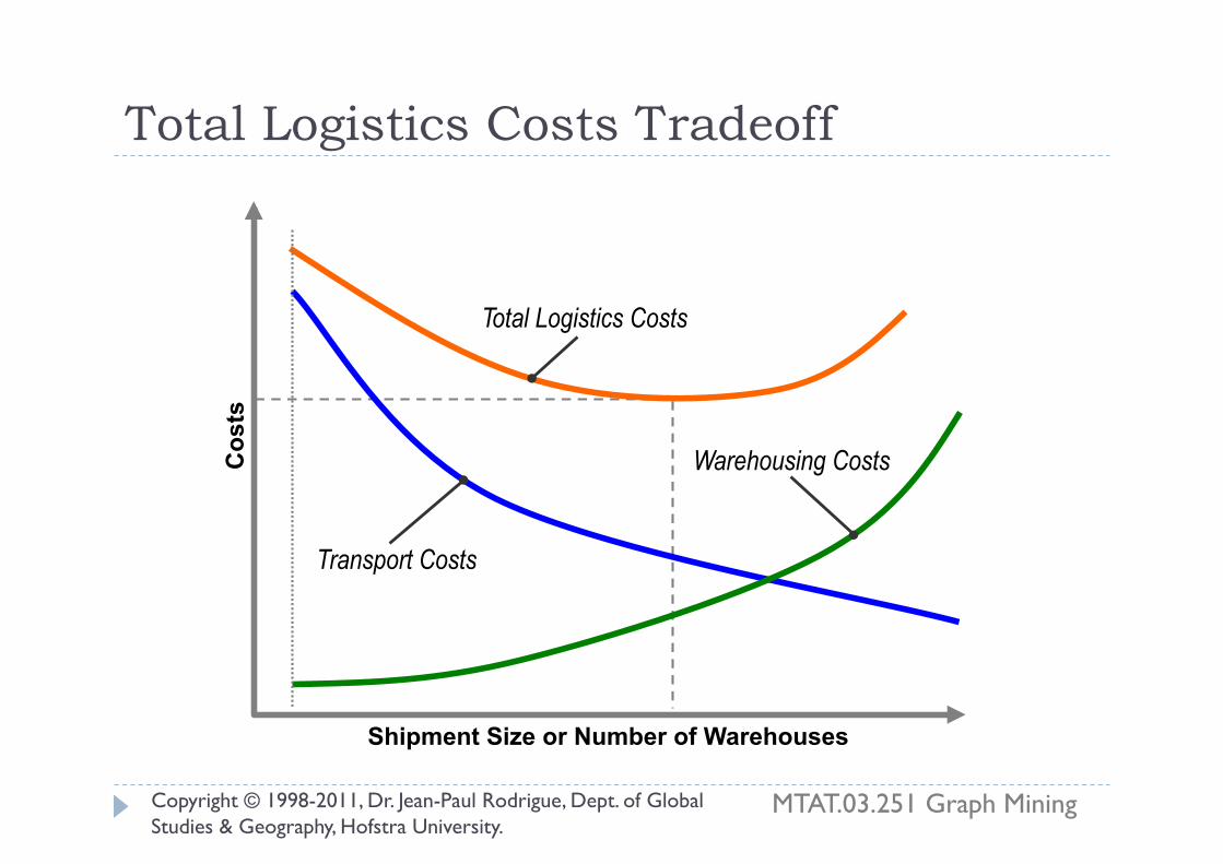
Total Logistics Costs Tradeoff
Copyright © 1998-2011, Dr. Jean-Paul Rodrigue, Dept. of Global Studies & Geography, Hofstra University.
Cos
ts
Shipment Size or Number of Warehouses
Transport Costs
Total Logistics Costs
Warehousing Costs
MTAT.03.251 Graph Mining

Additional Measurements Of Traffic Volume
C – cost associated with paths or links.
i.e. generalized cost (in transport economics)-is the sum of the monetary and non-monetary costs of a journey
Costs associated with QoS - quality of service (in computer and telecommunication networks ) is the ability to provide different priority to different applications, users, or data flows, or to guarantee a certain level of performance to a data flow
MTAT.03.251 Graph Mining

Characteristics Of The Network Flows How will traffic change over time?
MTAT.03.251 Graph Mining
Characteristics Of The Network Flows How will traffic change over time?
Time
MTAT.03.251 Graph Mining
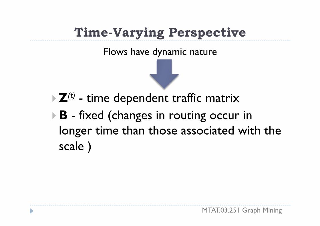
Time-Varying Perspective Flows have dynamic nature
Z(t) - time dependent traffic matrix B - fixed (changes in routing occur in
longer time than those associated with the scale )
MTAT.03.251 Graph Mining

Characteristics Summary Origin Destination
B – Routing Matrix
Z - Traffic Matrix
C - Cost
T - Time
FLOW
MTAT.03.251 Graph Mining

Flow analysis classification
Measurements Goal Method
OD flow volumes Zij Model observed flow volumes Zij
Gravity Models
Link volumes Xe Predict unobserved OD flow volumes Zij
Traffic matrix estimation(static, dynamic)
OD costs cij Predict unobserved OD and link costs
Estimation of network flow costs
MTAT.03.251 Graph Mining
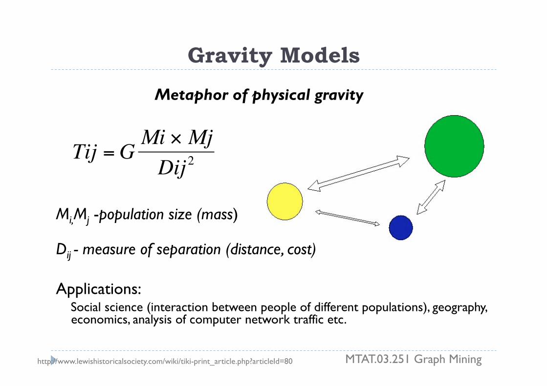
Gravity Models
Metaphor of physical gravity
Mi,Mj -population size (mass)
Dij - measure of separation (distance, cost)
Applications: Social science (interaction between people of different populations), geography, economics, analysis of computer network traffic etc.
MTAT.03.251 Graph Mining http://www.lewishistoricalsociety.com/wiki/tiki-print_article.php?articleId=80
€
Tij =G Mi × MjDij 2

Application of an Elementary Spatial Interaction Equation
W X Y Z Ti
W 100,000 100,000
X 100,000 50,000 25,000 175,000
Y 50,000 50,000
Z 25,000 25,000
Tj 100,000 175,000 50,000 25,000 350,000
€
Tij = kPi ∗Pj
Dij
Copyright © 1998-2011, Dr. Jean-Paul Rodrigue, Dept. of Global Studies & Geography, Hofstra University.
X
2,000,000
Y
Z W
800 km
400 km
2,000,000 1,000,000 k = 0.00001
(people per week)
2,000,000
Weight (P)
Distance (D)
Constant (k)
Centroid (i) Interaction (T)
Elementary Formulation
MTAT.03.251 Graph Mining

Relationship between Distance and Interactions
Copyright © 1998-2011, Dr. Jean-Paul Rodrigue, Dept. of Global Studies & Geography, Hofstra University.
Distance
Interaction
A B
A C
A D
A B C D
T(B-A)
T(C-A)
T(D-A)
MTAT.03.251 Graph Mining

General Gravity Model Specifies that the traffic flows Zij to be in the form of counts, with
independent Poisson distributions and the mean function of the form of:
Tij=E(Zij)- expected value of interaction hO(i)=Pi - origin function hD(j)=Pj- destination function hS(cij)=Dij - separation function cij- vector of K separation attributes
MTAT.03.251 Graph Mining
€
Tij = kPi ∗Pj
Dij
,where
Pi
2,000,000
Pj
Dij=800 km
2,000,000

Extension of the Gravity Model.
X
2,000,000
Y
Z W
800 km
400 km
2,000,000 1,000,000 k = 0.00001
(people per week)
2,000,000
Weight (P)
Distance (D)
Constant (k)
Centroid (i) Interaction (T)
W X Y Z Ti
W 71,378 71,378
X 6,059 2,203 36 8,298
Y 19,420 19,420
Z 153,893 153,893
Tj 6,059 244,692 2,203 36 252,990
€
Tij = kPiα ∗Pj
β
Dijθ
Simple Formulation
Exponent
λ = 0.95 α = 1.05
λ = 1.03 α = 0.96
λ = 1.2 α = 0.7
λ = 1.00 α = 0.90
Copyright © 1998-2011, Dr. Jean-Paul Rodrigue, Dept. of Global Studies & Geography, Hofstra University.
MTAT.03.251 Graph Mining

Extension of the Gravity Model. Power functions
MTAT.03.251 Graph Mining
€
hO (i) = (Pi)α = (πO ,i)α
€ Cij-scalar, θ ≥ 0
€
€
hD ( j) = (Pj)β = (πD j)β
€
hS (cij) = (Dij)−θ = (cij)−θ
,where
origin function
destination function
separation function
OR
flow
cost
~1/xa
~exp()
Gravity Models. Example Austrian Call Data
Need to understand the spatial structure of telecommunication interactions among populations between different geographical
regions
MTAT.03.251 Graph Mining
Gravity Models. Example Austrian Call Data
Need to understand the spatial structure of telecommunication interactions among populations between different geographical
regions
WHY?
MTAT.03.251 Graph Mining
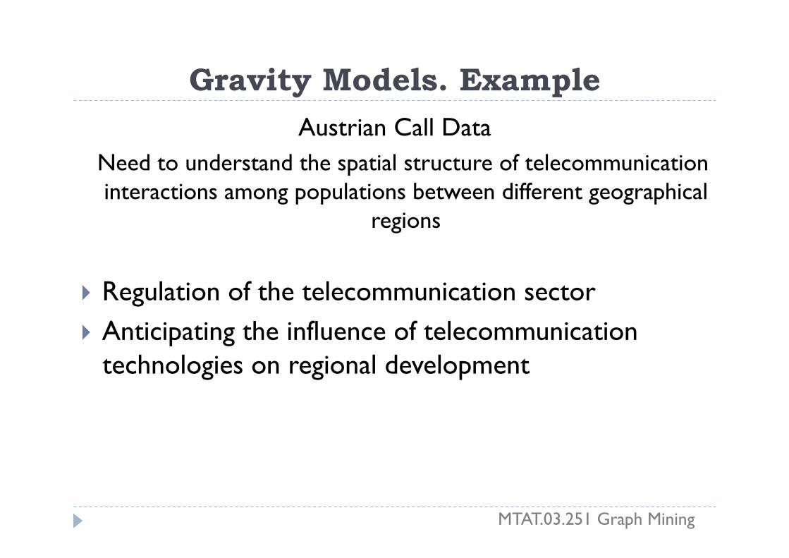
Gravity Models. Example Austrian Call Data
Need to understand the spatial structure of telecommunication interactions among populations between different geographical
regions
Regulation of the telecommunication sector Anticipating the influence of telecommunication
technologies on regional development
MTAT.03.251 Graph Mining
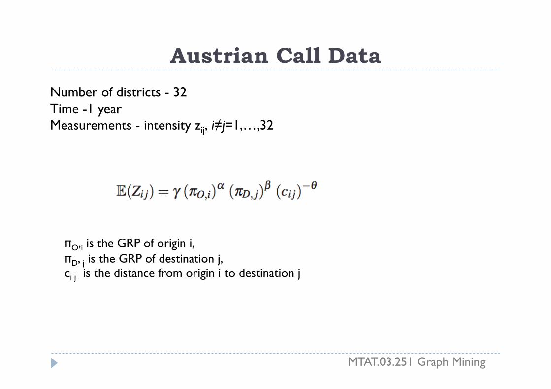
Austrian Call Data
MTAT.03.251 Graph Mining
Number of districts - 32 Time -1 year Measurements - intensity zij, i≠j=1,…,32
πO,i is the GRP of origin i, πD, j is the GRP of destination j, ci j is the distance from origin i to destination j

Austrian Call Data
Scatter plots: Call flow volume versus each of Origin GRP Destination GRP Distance
nonparametric smoother
linear regression
MTAT.03.251 Graph Mining

Alternative Representation. Interaction Probabilities
represent the expected relative frequency at which interactions are specifically ij-interactions
,where
Under the general gravity model specification they can be expressed as:
MTAT.03.251 Graph Mining

Alternative Representation. Destination Gravity Models
related to the counts of Zij from given origin i to all destinations j
Conditional destination probabilities:
In terms of components in general probabilities:
MTAT.03.251 Graph Mining
€
P(A |B) =P(A∩ B)P(B)

Inference For The Gravity Models
Zij – independent Poisson random variables with means:
General model specification:
,where
MTAT.03.251 Graph Mining
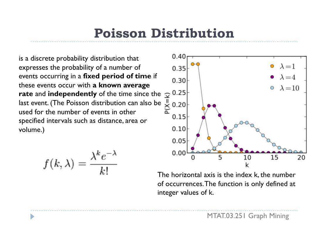
Poisson Distribution
The horizontal axis is the index k, the number of occurrences. The function is only defined at integer values of k.
is a discrete probability distribution that expresses the probability of a number of events occurring in a fixed period of time if these events occur with a known average rate and independently of the time since the last event. (The Poisson distribution can also be used for the number of events in other specified intervals such as distance, area or volume.)
MTAT.03.251 Graph Mining

Ma Given a sample of n measured values ki we wish to estimate the value of the parameter λ of the Poisson population from which the sample was drawn. To calculate the maximum likelihood value, we form the log-likelihood function
Take the derivative of L with respect to λ and equate it to zero:
Solving for λ yields a stationary point, which if the second derivative is negative is the maximum-likelihood estimate of λ:
Checking the second derivative, it is found that it is negative for all λ and ki greater than zero, therefore this stationary point is indeed a maximum of the initial likelihood function: MTAT.03.251 Graph Mining

Inference For The Gravity Models. Maximum Likelihood
Z = z be an (IJ)×1 vector of observations of the flows Zij, ordered by origin i, and by destination j within origin i
Poisson log-likelihood for μ:
maximum likelihood for estimates:
for μi j satisfys the equations:
,where
MTAT.03.251 Graph Mining

Example. Analysis Of The Austrian Call Data
MTAT.03.251 Graph Mining
consider two models
• Fitted using generic iteratively weighted least- squares method for generalized linear models
• Model arguments are considered significant at the 0,05 level
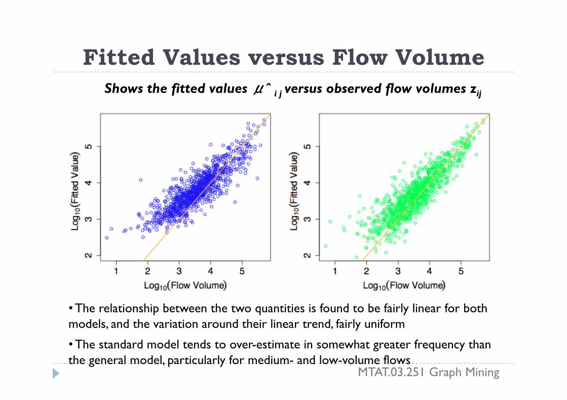
Fitted Values versus Flow Volume Shows the fitted values μˆ i j versus observed flow volumes zij
• The relationship between the two quantities is found to be fairly linear for both models, and the variation around their linear trend, fairly uniform
• The standard model tends to over-estimate in somewhat greater frequency than the general model, particularly for medium- and low-volume flows
MTAT.03.251 Graph Mining

Relative Error versus Flow Volume
light and dark points indicate under- and over- estimation, respectively
MTAT.03.251 Graph Mining
Shows the relative errors (zij-μˆij)/zij versus the flow volumes zij
• For both models the relative error varies widely in magnitude. • The relative error decreases with volume. • For low volumes both models are inclined to over-estimate, while for higher volumes, they are increasingly inclined to under-estimate.
Thank you for your attention!
MTAT.03.251 Graph Mining