Gravity changes over Russian rivers basins from GRACE

Leonid Zotov1,4, Natalya Frolova2, C.K. Shum3

1Sternberg Astronomical Institute, Moscow State University, Russia 2Department of Hydrology, Faculty of Geography, Moscow State University, Russia 3School of Earth Sciences, Ohio State University, USA 4Paris Observatory, France

20 May 2014 CNES, Toulouse, France

Satellites give hydrological data, which present in

Passive (SSM/I) and active (ERS) microwave radars data

Visual light and near infrared (AVHRR) images

Altimetry data (JASON, Envisat, ERS)

Atmospheric precipitation and humidity profiles

Gravity measurements (GRACE, GOCE)

Levels of rivers and lakes

Hydrological mass changes are related to

Snow cover

Water stored in soil and in biomass Precipitation

Gravity field studies can be useful for

Hydrological, meteorological, climatological research. For example, Climate Change influence river’s water balance, permafrost, changes water discharge to the ocean, sea level, water and ice regime of Arctica. Mass redistributions influence Earth rotation. The whole set of geodetic and geodynamical questions is involved. Their study could be important for rational natural resources management, construction, etc.

Soil moisture data (SMOS)

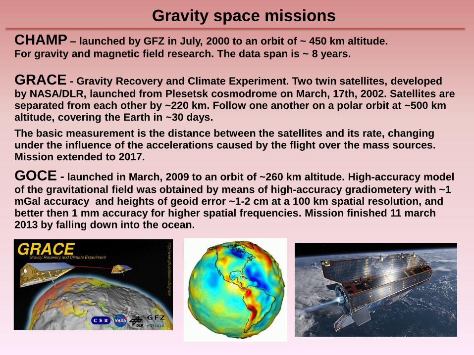
Gravity space missions

CHAMP – launched by GFZ in July, 2000 to an orbit of ~ 450 km altitude.

For gravity and magnetic field research. The data span is ~ 8 years.

GRACE - Gravity Recovery and Climate Experiment. Two twin satellites, developed

by NASA/DLR, launched from Plesetsk cosmodrome on March, 17th, 2002. Satellites are separated from each other by ~220 km. Follow one another on a polar orbit at ~500 km altitude, covering the Earth in ~30 days.

The basic measurement is the distance between the satellites and its rate, changing under the influence of the accelerations caused by the flight over the mass sources. Mission extended to 2017.

GOCE - launched in March, 2009 to an orbit of ~260 km altitude. High-accuracy model

of the gravitational field was obtained by means of high-accuracy gradiometery with ~1 mGal accuracy and heights of geoid error ~1-2 cm at a 100 km spatial resolution, and better then 1 mm accuracy for higher spatial frequencies. Mission finished 11 march 2013 by falling down into the ocean.

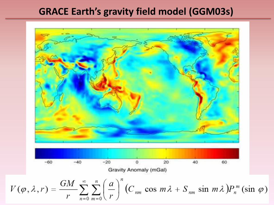
GRACE Earth’s gravity field model (GGM03s)

We used JPL Level-2 RL05 monthly GRACE spherical

harmonic data since 01.2003 till 12.2013 with coefficients

complete to degree and order 60.

Accumulator power shortage and economy caused absance of

data for some months. Only January (01.01-17.01) L2 file is

delivered in 2014.

Eight files (06.03, 01.11, 06.11, 05.12, 10.12, 03.13, 08.13,

09.13) were linearly interpolated (overall N=132 files used).

C20 coefficients were replaced by SLR-derived.

Average field over 10 years was subtracted.

GIA effect was removed according to Paulson 2007 model.

Results are represented in equivalent water height (EWH) level

(cm) according to equation

GRACE data preprocessing

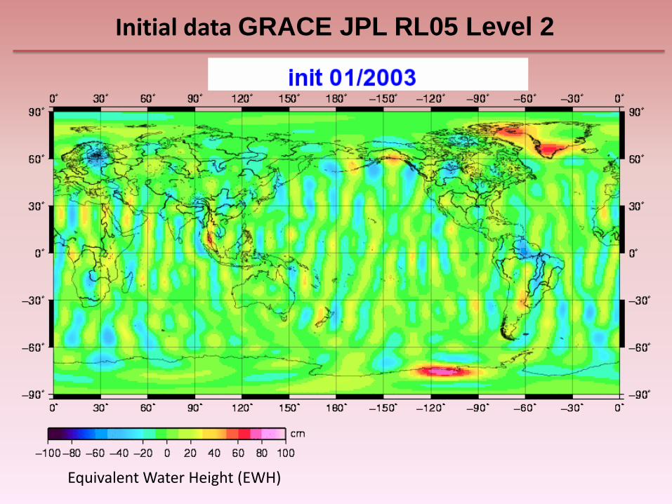
Initial data GRACE JPL RL05 Level 2

Equivalent Water Height (EWH)

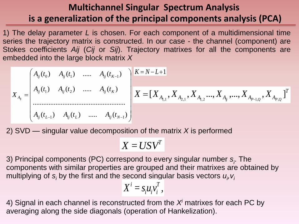
3) Principal components (PC) correspond to every singular number si. The

components with similar properties are grouped and their matrixes are obtained by multiplying of si by the first and the second singular basis vectors ui,vi

1) The delay parameter L is chosen. For each component of a multidimensional time series the trajectory matrix is constructed. In our case - the channel (component) are Stokes coefficients Aij (Cij or Sij). Trajectory matrixes for all the components are embedded into the large block matrix X

Multichannel Singular Spectrum Analysis is a generalization of the principal components analysis (PCA)

2) SVD — singular value decomposition of the matrix X is performed

4) Signal in each channel is reconstructed from the Xi matrixes for each PC by averaging along the side diagonals (operation of Hankelization).

,vus=X T

iii

i

TUSV=X

)(.....)()(

.....................................................

)(.....)()(

)(.....)()(

11

21

110

NijLijLij

Kijijij

Kijijij

A

tAtAtA

tAtAtA

tAtAtA

Xij

1 LNK

T

AAAAAA QPQPijXXXXXXX ],,...,...,,,[

,,12,11,21,1

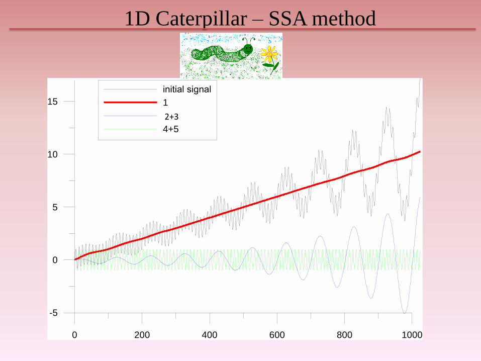
0 200 400 600 800 1000

-5

0

5

10

15

initial signal

1

3+4

4+5

1D Caterpillar – SSA method

2+3

MSSA of GRACE data – singular numbers L=48 months (4 years)

trend

Annual oscillation

L. Zotov, C.K. Shum. Singular spectrum analysis of GRACE observations, American Institute of Physics Proceedings, of the 9th Gamow summer school, 2009, Odessa, Ukraine.

Annual cycle – PC 1

МССА, L=48 months

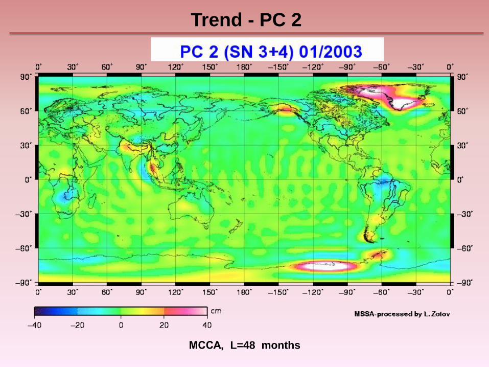
Trend - PC 2

МССА, L=48 months

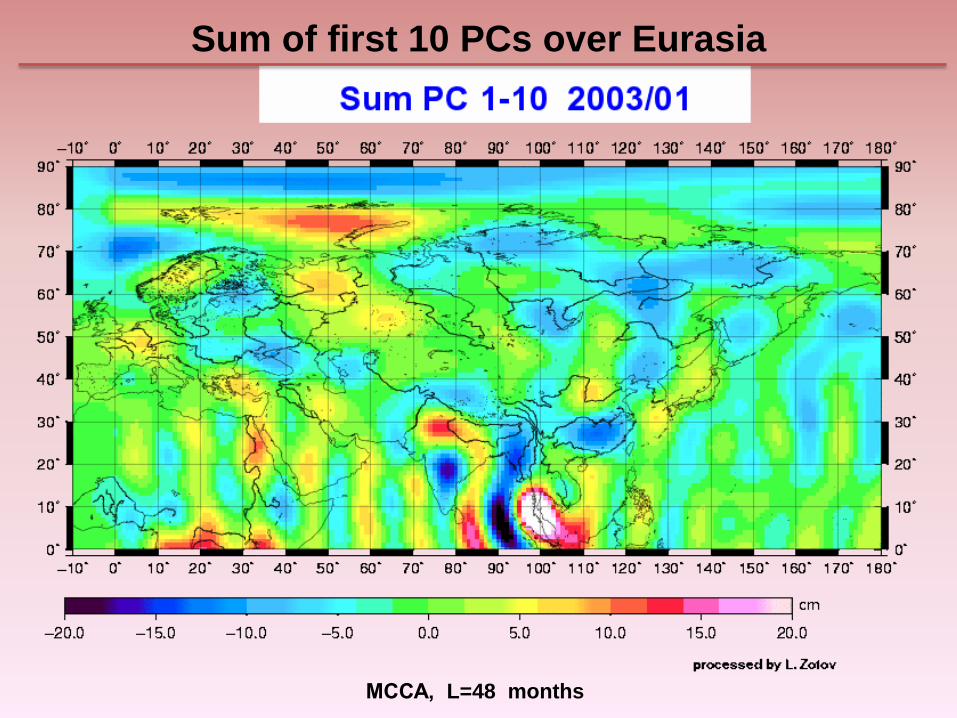
Sum of first 10 SNs

MSSA with L=36 months

Remaining components, sum SNs >10

МССА, L=48 months

МССА, L=48 months

Sum of first 10 PCs over Eurasia

100 200 300 400 500 600 700

50

100

150

200

250

300

350

100 200 300 400 500 600 700

50

100

150

200

250

300

350

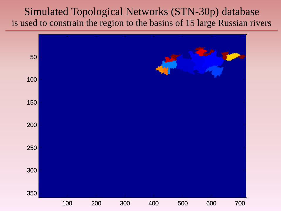
Simulated Topological Networks (STN-30p) database is used to constrain the region to the basins of 15 large Russian rivers

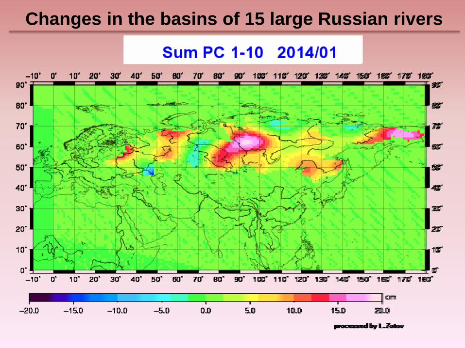
Changes in the basins of 15 large Russian rivers

Mass anomaly (averaged field) in the basins of 15 large Russian rivers

cm

Mass anomaly (averaged field) in the basins of 15 large Russian rivers

Comparison with CNES/GRGS RL 03 for Moscow

CNES and JPL data from http://www.thegraceplotter.com/

Averaged annual cycle over the basins of 15 large Russian rivers

The differences for the annual PC 1 between monthly (March-June 2013) maps and average maps over 9 years (2003-2012) for the corresponding months.

Positive anomalies in spring 2013 over Russia depicts anomalous snow accumulation.

Annual cycle anomalies for March-June

300 km gaussian smoothing, GIA subtracted, Map from http://geoid.colorado.edu/grace/dataportal.html

Averaged trend over the basins of 15 large Russian rivers

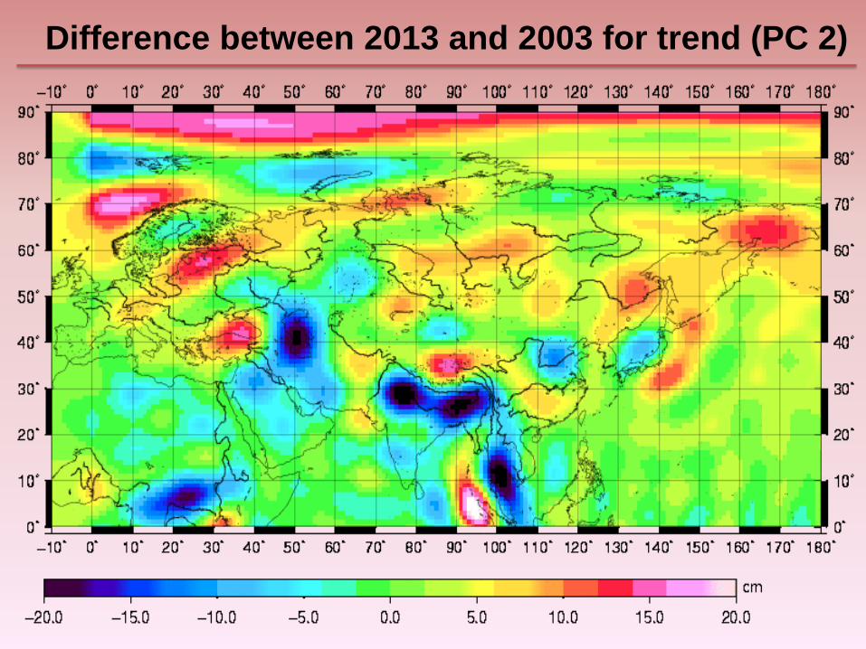
Difference between 2013 and 2003 for trend (PC 2)

25 km gaussian filter, GIA subtracted, map from http://geoid.colorado.edu/grace/dataportal.html

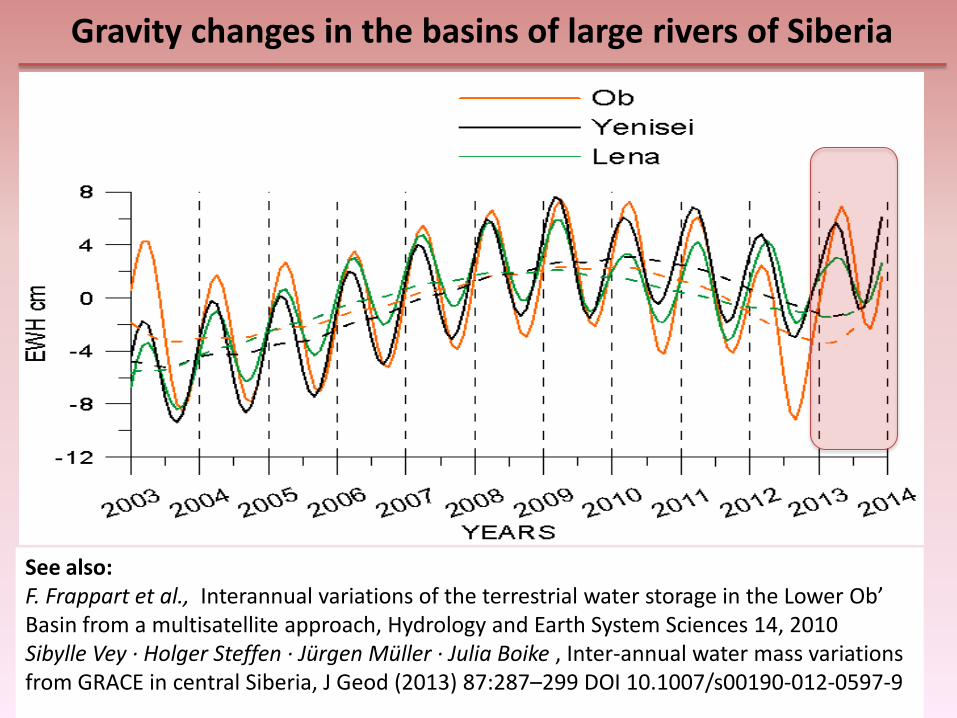
Gravity changes in the basins of large rivers of Siberia

See also: F. Frappart et al., Interannual variations of the terrestrial water storage in the Lower Ob’ Basin from a multisatellite approach, Hydrology and Earth System Sciences 14, 2010 Sibylle Vey · Holger Steffen · Jürgen Müller · Julia Boike , Inter-annual water mass variations from GRACE in central Siberia, J Geod (2013) 87:287–299 DOI 10.1007/s00190-012-0597-9

CNES and JPL plots from http://www.thegraceplotter.com/

Comparison with CNES/GRGS RL 03 for Ob basin

Gravity changes in the basins of large rivers of Russian North and Far East

Comparison with CNES/GRGS RL 03 data For Amur river basin

CNES and JPL data from http://www.thegraceplotter.com/

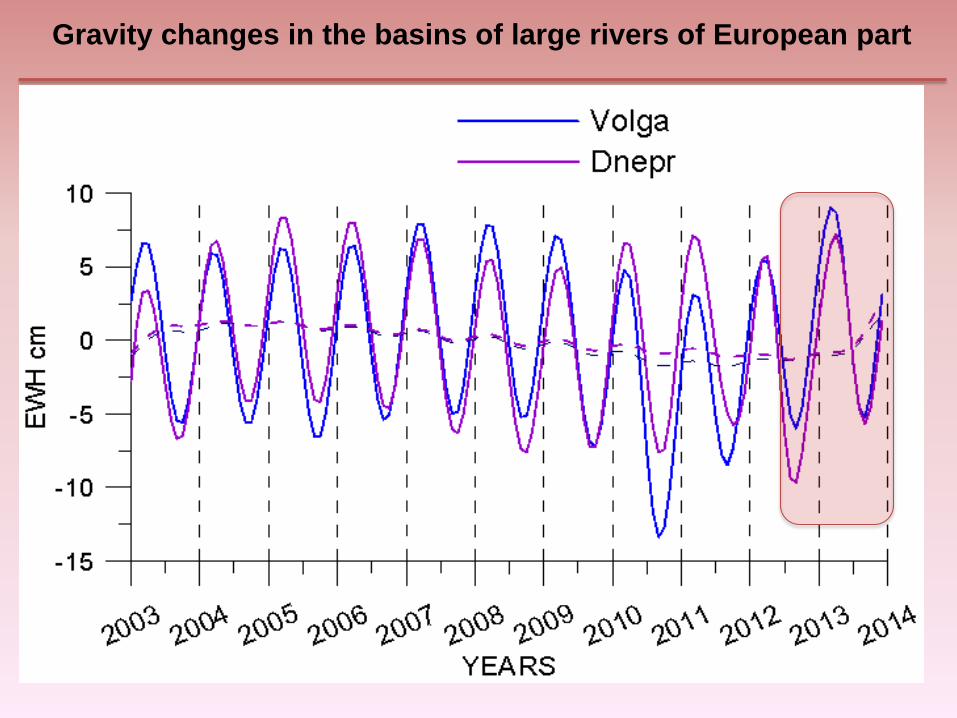
Gravity changes in the basins of large rivers of European part

CYMENT data from http://www.legos.obs-mip.fr/soa/hydrologie/hydroweb/

ENVISAT measurements

Gravity measurements

Comparison with data from hydrological web CYcle de l’eau et de la Matière dans les bassins vErsaNTs (CYMENT)

for Volga basin

Anomalous heat wave in Moscow, Russia 20-27 July 2010 Compared to average over 2000-2008, MODIS, Terra

Will the heat repeats in 2014 ?

Volga, Astrakhan

Volga, Volgograd

Amur, Khabarovsk

Dnepr, Bolshevo

cm

cm

River’s level changes from the Cadastr Center of Russia

Volga, Astrakhan

Volga, Volgograd

Amur, Khabarovsk

Dnepr, Bolshevo

cm

Vous n’aures auncune donnees (pas de gaz sans argent)

Mass balance equation

ΔTWS = ΔSW+ Δ(P-E) + ΔSN + ΔTSS - ΔR, where ΔTWS – measured by GRACE

ΔSW – changes in lakes and swamps Δ(P-E) – changes of precipitation–evaporation difference ΔSN – snow cover storage changes ΔTSS – ground water storage changes ΔR – river discharge changes

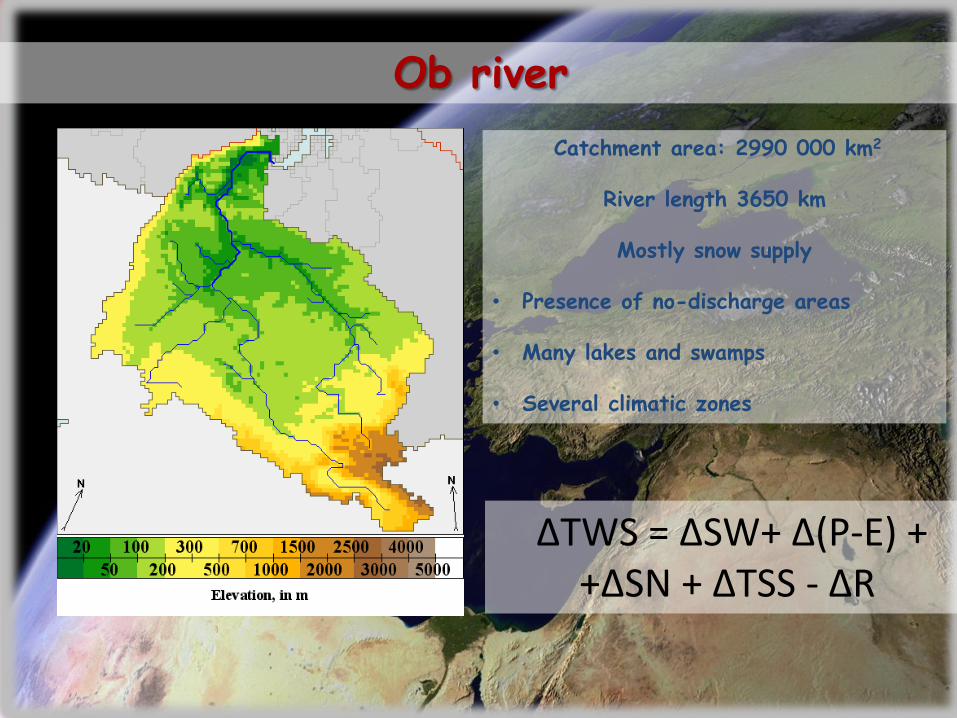
Ob river

ΔTWS = ΔSW+ Δ(P-E) + +ΔSN + ΔTSS - ΔR

Сatchment area: 2990 000 km2

River length 3650 km

Mostly snow supply

• Presence of no-discharge areas

• Many lakes and swamps

• Several climatic zones

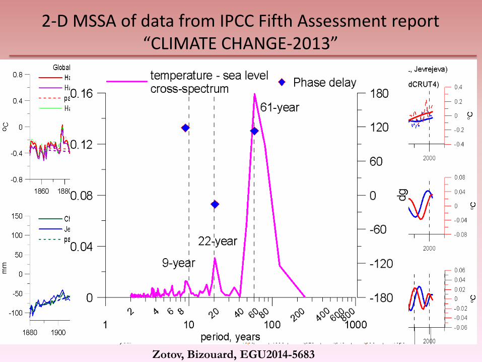
2-D MSSA of data from IPCC Fifth Assessment report “CLIMATE CHANGE-2013”

Zotov, Bizouard, EGU2014-5683

HadCRUT4 after trend subtraction and Length of Day LOD

Correlation 0.43-0.55

years

Are Earth rotation and Climate Change related? This question already posed in K. Lambeck (1980) monograph.

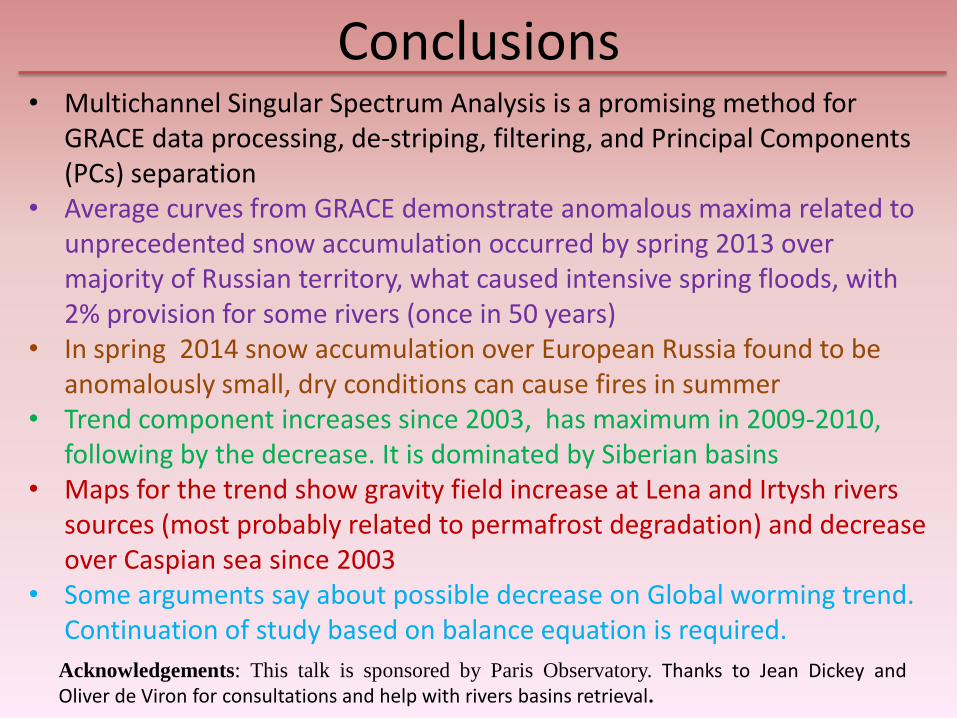
Conclusions • Multichannel Singular Spectrum Analysis is a promising method for

GRACE data processing, de-striping, filtering, and Principal Components (PCs) separation

• Average curves from GRACE demonstrate anomalous maxima related to unprecedented snow accumulation occurred by spring 2013 over majority of Russian territory, what caused intensive spring floods, with 2% provision for some rivers (once in 50 years)

• In spring 2014 snow accumulation over European Russia found to be anomalously small, dry conditions can cause fires in summer

• Trend component increases since 2003, has maximum in 2009-2010, following by the decrease. It is dominated by Siberian basins

• Maps for the trend show gravity field increase at Lena and Irtysh rivers sources (most probably related to permafrost degradation) and decrease over Caspian sea since 2003

• Some arguments say about possible decrease on Global worming trend. Continuation of study based on balance equation is required.

Acknowledgements: This talk is sponsored by Paris Observatory. Thanks to Jean Dickey and Oliver de Viron for consultations and help with rivers basins retrieval.

Merci pour votre attention!

Photo by Irina Repina