CTPU-17-26KEK-TH-1986

Gravitational waves from bubble dynamics:

Beyond the Envelope

Ryusuke Jinnoa,b and Masahiro Takimotob,c

a Center for Theoretical Physics of the Universe, Institute for Basic Science (IBS),Daejeon 34051, Korea

b Theory Center, High Energy Accelerator Research Organization (KEK),Oho, Tsukuba, Ibaraki 305-0801, Japan

c Department of Particle Physics and Astrophysics, Weizmann Institute of Science,Rehovot 7610001, Israel

Abstract

We study gravitational-wave production from bubble dynamics (bubble collisionsand sound waves) during a cosmic first-order phase transition with an analytic ap-proach. We model the system with the thin-wall approximation but without the en-velope approximation often adopted in the literature. We first write down analyticexpressions for the gravitational-wave spectrum, and then evaluate them with numer-ical methods. It is found that, in the long-lasting limit of the collided walls, thespectrum grows from ∝ f3 to ∝ f1 for low frequencies, showing a significant enhance-ment compared to the one with the envelope approximation. It is also found thatthe spectrum saturates in the same limit, indicating a decrease in the correlation ofthe energy-momentum tensor at late times. The bubble walls in our setup are con-sidered as modeling the scalar field configuration and/or the bulk motion of the fluid,and therefore our results have implications to gravitational-wave production from bothbubble collisions (scalar dynamics) and sound waves (fluid dynamics).

arX

iv:1

707.

0311

1v1

[he

p-ph

] 1

1 Ju

l 201

7

Contents

1 Introduction 1

2 Setup and basic ingredients 22.1 Bubble dynamics in cosmological phase transitions . . . . . . . . . . . . . . . 32.2 Explicit form of the energy-momentum tensor . . . . . . . . . . . . . . . . . 112.3 Nucleation rate of bubbles . . . . . . . . . . . . . . . . . . . . . . . . . . . . 122.4 GW power spectrum from the energy-momentum tensor . . . . . . . . . . . 13

2.4.1 GW power spectrum at the transition time . . . . . . . . . . . . . . . 132.4.2 GW power spectrum at present . . . . . . . . . . . . . . . . . . . . . 16

2.5 Summary of the setup and its physical implications . . . . . . . . . . . . . . 16

3 Analytic expressions 173.1 Basic strategy . . . . . . . . . . . . . . . . . . . . . . . . . . . . . . . . . . . 173.2 Analytic expressions . . . . . . . . . . . . . . . . . . . . . . . . . . . . . . . 18

4 Numerical results 194.1 Spectral shape . . . . . . . . . . . . . . . . . . . . . . . . . . . . . . . . . . . 194.2 Peak position . . . . . . . . . . . . . . . . . . . . . . . . . . . . . . . . . . . 20

5 Discussion and conclusions 25

A GW spectrum with the envelope approximation 29A.1 Basic strategy . . . . . . . . . . . . . . . . . . . . . . . . . . . . . . . . . . . 29A.2 Prerequisites . . . . . . . . . . . . . . . . . . . . . . . . . . . . . . . . . . . . 30A.3 Single-bubble spectrum . . . . . . . . . . . . . . . . . . . . . . . . . . . . . . 34A.4 Double-bubble spectrum . . . . . . . . . . . . . . . . . . . . . . . . . . . . . 37

B GW spectrum beyond the envelope approximation 41B.1 Basic strategy . . . . . . . . . . . . . . . . . . . . . . . . . . . . . . . . . . . 41B.2 Prerequisites . . . . . . . . . . . . . . . . . . . . . . . . . . . . . . . . . . . . 41B.3 Single-bubble spectrum . . . . . . . . . . . . . . . . . . . . . . . . . . . . . . 44B.4 Double-bubble spectrum . . . . . . . . . . . . . . . . . . . . . . . . . . . . . 47

C Derivation of the simplification formulas 53C.1 Single-bubble simplification formula . . . . . . . . . . . . . . . . . . . . . . . 53C.2 Double-bubble simplification formula . . . . . . . . . . . . . . . . . . . . . . 56

D Techniques for numerical evaluation 63D.1 Equivalent ways to impose the spacelike conditions . . . . . . . . . . . . . . 63D.2 〈T (x)〉 〈T (y)〉 subtraction . . . . . . . . . . . . . . . . . . . . . . . . . . . . . 66

E Analytic proof on the spectrum behavior 71E.1 Single-bubble spectrum . . . . . . . . . . . . . . . . . . . . . . . . . . . . . . 71E.2 Double-bubble spectrum . . . . . . . . . . . . . . . . . . . . . . . . . . . . . 72

1

F Useful equations 76

G Other numerical results 76

H Comment on “spherical symmetry” 77

1 Introduction

Gravitational waves (GWs) provide us with a unique probe to the early universe. Variouscosmological dynamics are known to produce GWs: inflationary quantum fluctuations [1],preheating [2], topological defects such as domain walls and cosmic strings [3], and first-orderphase transitions [4,5]. Gravitational waves from these cosmological sources, if detected, willgive us an important clue to the high energy physics we are seeking for. On the observationalside there has recently been a great progress of the detection of GWs from black hole binariesby the LIGO collaboration [6–8], and gravitational-wave astronomy has now been established.In the future, space interferometers such as LISA [9], BBO [10] and DECIGO [11] areexpected to open up the era of gravitational-wave cosmology.

In this paper, we study GW production from first-order phase transitions. Though it hasbeen shown that first-order phase transitions do not occur within the standard model [12–14],there are various types of motivated particle physics models which predict first-order phasetransitions (see e.g. Refs. [15,16]). Excitingly, planned GW detectors are sensitive to phasetransitions around TeV-PeV scales, and thus such GWs offer one of the promising tools toprobe new physics beyond the standard model.

In a thermal first-order phase transition, true-vacuum bubbles start to nucleate at sometemperature, and then they expand because of the pressure difference between the falseand true vacua. These bubbles eventually collide with each other and the phase transitioncompletes. Even though uncollided bubbles do not radiate GWs because of the sphericalsymmetry of each bubble, the collision process breaks the symmetry and as a result GWs areproduced. The analysis of GW production from such processes was initiated in Refs. [17–20].In the first numerical simulation carried out in Ref. [17] in a vacuum transition, it was no-ticed that the main GW production comes from the uncollided regions of the bubble walls.This observation made the basis for the “envelope approximation,” in which only the un-collided regions of the bubble walls are taken into account in calculating GW production(see Fig. 1). This approximation has been widely used in the subsequent literature togetherwith the “thin-wall approximation,” in which the released energies are assumed to be con-centrated in an infinitesimally thin bubble walls.♦1 Later a numerical simulation with thesame approximations has been performed in Ref. [21] with an increased number of bubbles,and a more precise form of the GW spectrum has been obtained.

In the literature mentioned above, the bubble walls are thought to represent the energyconcentration by the profile of the scalar field that drives the transition or by the bulkmotion of the fluid coupled to the scalar field. It has recently been noticed in a series ofnumerical simulations [22–24]♦2 that the latter bulk motion propagates even after bubblecollisions, and works as a long-lasting source of GWs. It has been found that the GWs fromsuch sound waves typically dominate the other sources of GWs,♦3 and that the resulting

♦1 Though in the early literature the envelope approximation includes the thin-wall approximation [17–20],we distinguish them in this paper.♦2 See also Refs. [25–27] for other numerical simulations.♦3 In addition to bubble collisions and sound waves, turbulence is another important source for GWs [20,

28–32]. Note that the sound-wave regime as we study in this paper can develop into turbulent regime atlate times.

1

spectrum cannot be modeled by the envelope approximation because of the long-lastingnature of the source [22–24,33].

These numerical simulations have brought significant developments in our understandingon GW sourcing both from bubble collisions and from sound waves. In this paper, however,we stress the importance of the cooperation between

Analytic understanding & Numerical understanding

of such a process, and aim to develop the former. This is partly because the former approachsometimes goes beyond the barrier of computational resources, and also because it oftenoffers a clearer understanding of the physics.♦4 For this purpose we adopt the method ofrelating the GW spectrum with the two-point correlator of the energy-momentum tensor〈T (x)T (y)〉, the method pioneered in Ref. [35]. In Ref. [36] it has been pointed out that,under the thin-wall approximation, various contributions to the correlator 〈T (x)T (y)〉 reduceto finite number of classes. This observation has made it possible in Ref. [36] to write downthe GW spectrum analytically in the same setup as the numerical study in Ref. [21], i.e. theGW spectrum with the thin-wall and envelope approximations.♦5 In this paper we furtherdevelop this method, and write down

Gravitational-wave spectrum with the thin-wall approximationbut without the envelope approximation.♦6

The bubble walls in our setup can be regarded as modeling the energy concentration in thescalar field and/or in the bulk motion of the fluid, and therefore the resulting spectrumis considered to be relevant to GW production both from bubble collisions (scalar fieldcontribution) and sound waves (fluid contribution). The analytic expressions for the GWspectrum, Eqs. (3.2) and (3.3), have multi-dimensional integrations, and hence we evaluatethem with numerical methods.♦7 As a result, the growth and saturation of the spectrum areclearly observed as a function of the duration time of the collided walls.

The organization of the paper is as follows. In Sec. 2 we present out setup and summarizebasic ingredients to estimate the GW spectrum. We also discuss the applicability of our setupin this section. In Sec. 3 we write down the analytic expressions for the GW spectrum, andwe evaluate them in Sec. 4 with Monte-Carlo integration. Sec. 5 is devoted to discussionand conclusions.

2 Setup and basic ingredients

In this section, we present our setup and basic ingredients to estimate the GW spectrum.In order to estimate the spectrum, we have to clarify the energy-momentum tensor of thesystem. It is determined by

♦4 There are attempts to understand GW production from sound waves using the sound-shell model [34].♦5 By using the same formalism, it is also possible to investigate analytically the effect of the bubble

nucleation rate or the cosmic expansion on the GW spectrum [37].♦6 There are other assumptions and approximations such as constant wall velocity, free propagation after

collision, and the absence of cosmic expansion. See Sec. 2.♦7 Note that this is essentially different from numerical simulations.

2

(1) Spacetime distribution of bubbles (i.e., nucleation rate of bubbles),

(2) Energy-momentum tensor profile around a bubble wall,

(3) Dynamics after bubble collisions.

Since it is generically hard to solve the full dynamics of the system, some reasonable approx-imations are necessary for practical calculations. The aim of the following subsections is toclarify the approximations and their validity.

In Sec. 2.1, we give a brief overview of bubble dynamics in a cosmological phase transition,and explain our approximations for (2) and (3) referring to their validity. In this subsectionwe do not show the explicit expression for the energy-momentum profile in order to avoidpossible complications. In Sec. 2.2, we present the explicit form of the profile. In Sec. 2.3, wegive our assumptions about the transition rate which determine (1). In Sec. 2.4, we presenta formalism to calculate the GW spectrum from the correlation function of the energy-momentum tensor. In Sec. 2.5 we summarize our setup and discuss its physical implications.

Before moving on, we comment on the meaning of “wall” in the present paper. This wordusually refers to the energy localization in the form of scalar field gradient. We use the word“scalar wall” for such energy localization when we give general discussions about the bubbledynamics in Sec. 2.1. However, as mentioned in Sec. 1, the main energy carrier aroundbubbles can be not only the scalar field but also the bulk motion of the fluid. Therefore,after modeling the energy-momentum profile in Sec. 2.2, we refer to such energy localizationas “wall.”

2.1 Bubble dynamics in cosmological phase transitions

In this subsection we give a brief overview on GW production in a cosmological phasetransition paying particular attention to the bubble dynamics. We also introduce our ap-proximations for (2) and (3) and discuss their validity.

Classification

In cosmological first-order phase transitions, bubbles of the true vacuum nucleate, expandand then collide with each other. The released free energy accumulates around them dur-ing their expansion. Though uncollided bubbles do not radiate GWs due to the sphericalsymmetry of each bubble, their collisions break it and produce GWs. In order to estimatethe resulting GW spectrum, we have to know the energy-momentum tensor of the systemdetermined by the bubble dynamics. Depending on the system, bubble dynamics can becategorized into three classes:

(a) Runaway,

(b) Low terminal velocity,

(c) High terminal velocity.

3

Roughly speaking, the balance between the released energy and the friction due to back-ground thermal plasma determines which case is realized (see e.g. Refs. [38,39]). Schemati-cally, the acceleration of the scalar wall is given by

vw ∝ ρ0 − Ffric(vw), (2.1)

where vw is the scalar wall velocity, ρ0 denotes the released energy, and Ffric(vw) denotes thefriction term.

In the non-relativistic regime, the friction term is proportional to the velocity: Ffric ∝ vw.If the ratio between the released energy and that of the surrounding plasma ρrad:

α ≡ ρ0

ρrad

. (2.2)

is suppressed α . O(0.1), the acceleration tends to cease within non-relativistic regime.♦8

We refer to such cases as (b) low terminal velocity. On the other hand, if the released energyis large enough α & O(0.1), the scalar wall velocity enters the relativistic regime vw ' 1.In order to deal with this regime, we have to know the behavior of the friction term inγw ≡ 1/

√1− v2

w →∞ limit. Though it had long been considered that the friction saturatesin the relativistic limit and cannot stop the acceleration of the scalar wall [40], the authors ofRef. [41] have recently pointed out that particle splitting processes around the wall generatea friction term proportional to γw. This term becomes larger and larger in γw → ∞ limit,and stops the acceleration before bubble collisions in some cases. In fact, as we discuss inSec. 2.1 (c), the acceleration may stop due to this splitting process for most cases of ourinterest. We refer to such cases as (c) high terminal velocity. We also denote by (a) runawaythose cases in which the acceleration continues until bubble collisions. Though such casesmay hardly occur in realistic setups, we nevertheless consider them in the following for aninstructive purpose: in fact, the dynamics is relatively simple and a clear prediction of theresulting GW spectrum is possible in runaway cases.

As mentioned in the beginning of this section, in order to have the energy-momentumtensor of the system, we have to clarify

(2) Energy-momentum tensor profile around a bubble wall,

(3) Dynamics after bubble collisions,

for each of (a), (b) and (c). Especially, the importance of (3) has recently been pointed outin Refs. [22–24], in which a sizable GW production from sound waves after bubble collisionshas been observed in numerical simulations. In this paper, we adopt

(2) Thin-wall approximation,

(3) Free propagation,

♦8 In order to determine the terminal velocity, we have to specify couplings between the scalar field andthe plasma. Here we do not consider details of friction, assuming that the couplings are not so suppressed.

4

for these two. The former assumes that the released energy is localized in an infinitesi-mally thin surface of a bubble, while the latter assumes that the energy and momentumaccumulated around a bubble until the first collision just pass through after that. Fig. 2 isa schematic picture of the system with these approximations. The black lines denote thethin walls, which model the energy and momentum localization in the scalar wall and/orin the bulk motion of the fluid. They accumulate more and more energy until their firstcollisions. On the other hand, the gray lines denote the evolution of such localized energyand momentum after collisions. They gradually lose the energy and momentum densitiesafter collisions as a result of free propagation. See also Eq. (2.19) for the explicit form ofthe energy-momentum tensor. In addition, we assume that the velocity of the propagationof the localized energy is constant both before and after collisions, and denote it by v. Be-low we discuss the validity of such approximations (thin-wall and free propagation with aconstant velocity) for both (a) and (b). Unfortunately, we do not know much about thedynamics realized in case (c). Thus, we only mention some features and possible proceduresto determine the GW spectrum in this case. We summarize properties of these cases inTable 1.

Before moving on, we comment on turbulence after bubble collisions. In all of the threecases plasma turbulence can be a sizable source for GWs at late times [20, 28–32]. How-ever, since the turbulence dynamics is highly nonlinear, we restrict ourselves to the bubbledynamics before the onset of turbulence in this paper.

Table 1: Classification of bubble dynamics

Type Width of source Scalar wall velocity Dynamics after collision

Runaway thin γw 1 free propagation with speed of lightLow terminal velocity thick constant vw free propagation with speed of soundHigh terminal velocity thick? constant γw 1 ?

(a) Runaway

In the runaway case the released energy is relatively large (α & O(0.1)) and the friction termcannot stop the acceleration of the scalar wall by the time of collisions. Below we assumethat the friction due to the surrounding plasma, especially the splitting effect explained in(c) high terminal velocity, is negligible. Though this case might be unrealistic, we considerit because this is one of the simplest setups where we can predict the GW spectrum ratherprecisely.

In the runaway case, the released energy accumulates around a thin surface of a bubblein the form of scalar gradient. Let us first consider the behavior of the scalar field beforecollisions. Suppose that the scalar field difference between the true and false vacua is ∆φ,the released energy density is ρ0, the bubble radius is R, and the width of energy localizationis lb. We may estimate the width of the surface as(

∆φ

lb

)2

lbR2 ∼ ρ0R

3 → lb ∼∆φ2

ρ0R. (2.3)

5

Figure 1: Rough sketch of bubble dynamics with the envelope approximation. The bubble walls,denoted by the black lines, accumulate energy and momentum as they expand and then lose theminstantly when they collide with others. Compare with Fig. 2. This figure is the same as in Ref. [36].

Figure 2: Rough sketch of bubble dynamics without the envelope approximation. The collidedbubble walls, denoted by the gray lines, gradually lose their energy and momentum densities aftercollisions.

6

Note that the width of the scalar gradient becomes thiner and thiner as bubbles expand.As we see in Sec. 2.3, the typical bubble size just before collision is sub-horizon, which wedenote Rcoll = ε/H with ε . O(0.1) and H denoting the Hubble parameter. For clarity, weparametrize ρ0 as ρ0 ∼ m2

typ∆φ2 where mtyp denotes a typical mass scale of the potential.Usually mtyp ∼ T holds with T being the temperature of the plasma. Also mtyp ∼ T . ∆φholds for most of the runaway cases since the released energy dominates over the radiationenergy. The typical momentum kb of the scalar field configuration carries just before collisionis given by

kb ∼1

lb

∣∣∣∣R=Rcoll

∼ εMP

(mtyp

∆φ

), (2.4)

where MP denotes the reduced Planck mass and we have used the Friedmann equationM2

PH2 ∼ ρ0 satisfied in the runaway case. Note that the typical momentum is much larger

than other physical parameters such as mtyp as long as the phase transition occurs well belowthe Planck scale. The number density nb of such high momentum modes just before collisionis given by

kbnblbR2coll ∼ ρ0R

3coll → nb ∼ εMPmtyp∆φ. (2.5)

Now let us consider the effect of bubble collisions. We focus only on those high momentummodes where most of the released energy is accumulated. Though the scalar field profile isdeformed to some extent during the collision process, deformation in such high momentummodes is expected to be small. To see this, let us consider a scattering process caused by λφ4

interaction for example. Denoting the change in the number density of such high momentummodes by ∆nb, we have the following relation:

∆nbnb∼ λ2

k2b

nb∆tcoll, ∆tcoll ∼1

lb→ ∆nb

nb∼ λ2

ε2

(∆φ

mtyp

)(H

MP

) 1, (2.6)

with ∆tcoll indicating the duration time of the collision process. We see that the effect ofcollision is typically negligible for the high momentum modes because of the last factor.

Next let us consider the effect of decay processes after bubble collisions. Denoting themass and decay rate of the scalar field at the true vacuum by ∼ mtyp and ∼ y2mtyp, respec-tively, we may estimate the lifetime of high momentum modes ∆tdecay as

H∆tdecay ∼ε

y2. (2.7)

Therefore the lifetime can be comparable to the Hubble time, though it depends on themodel parameters.

Finally let us consider the validity of the thin-wall approximation after collisions. Afterbubbles collide with each other, the energy injection into the scalar motion ceases andthe scalar field start to evolve with free propagation. Since the scalar motion has a finitemomentum width ∆kb, the width of the energy concentration becomes thicker and thicker.On the other hand, the relevant scale in the GW spectrum is the typical bubble size around

7

the time of collisions. Therefore, the thin-wall approximation is expected to hold untilthe width of the energy concentration becomes comparable to this length scale. Let usdenote by ∆tthin the timescale with which the scalar wall width grows to this length scale.Approximating the momentum width by ∆kb ∼ kb, we may estimate ∆tthin as♦9

∆tthink2b

m2typ

∼ Rcoll → H∆tthin ∼ ε

(kbmtyp

)2

1. (2.9)

Hence, the thin-wall approximation typically remains valid during a Hubble time as long asthe phase transition occurs much below the Planck scale.

Let us summarize the runaway case. During bubble expansion, the released energyaccumulates within extremely thin regions in the form of scalar gradient, and the scalar fieldbecomes ultra-relativistic. The effect of bubble collisions is typically negligible for such ultra-relativistic modes, and the walls are almost luminal both before and after collisions. Theuniverse becomes radiation dominated after the transition since the energy is dominatedby such ultra-relativistic modes. From these considerations we conclude that in runawaycase our assumptions (thin-wall and free propagation with a constant velocity) capture thebubble dynamics quite well.

(b) Low terminal velocity

Next let us consider those cases where the released energy is subdominant compared to thatof radiation (α . O(0.1)). In such cases, the dynamics of bubble expansion is determined bycoupled equations between the scalar field and the plasma. Soon after bubbles nucleate, thepressure difference between the true and false vacua gets balanced with the friction from thethermal plasma, and as a result the scalar wall velocity vw approaches a constant value [38].

During bubble expansion, the released energy is converted into the bulk motion of theplasma surrounding the scalar wall. Since there is no distance scale in the fluid equations,the fluid profile (enthalpy ω, fluid velocity u and so on) depends only on the variable ξ ≡ r/t,where r is the distance from the bubble nucleation point and t is the time after nucleation.Generally the fluid bulk motion is localized around the position of the scalar wall ξ ∼ vw,♦10

and the width of this energy localization is smaller than but comparable to the bubble size.The fraction κ of the released energy ρ0 which goes into the plasma motion is obtained as

κ =3

ρ0v3w

∫ ∞0

dξ ξ2ωγ2u2, (2.10)

with γ ≡ 1/√

1− u2, and is called the efficiency factor.After bubble collisions, the energy injection into plasma motion ceases. However, as

pointed out in Refs. [22–24], the plasma motion remains after bubble collisions and such

♦9 This can be estimated from the relation between the velocity dispersion and the momentum dispersion:

∆γw ∼vw∆vw

(1− v2w)3/2∼ ∆kbmtyp

. (2.8)

♦10 Note that this does not necessarily mean that the fluid velocity u is close to the scalar wall velocity vw.

8

remaining motions can produce a sizable amount of GWs. In the present case the releasedenergy is typically subdominant compared to the plasma energy density, and thus δρ/ρrad 1 hold in most cases with δρ ∼ κρ0 being the energy density in the plasma motion localizedaround the bubbles. Also, the fluid velocity u is at most of order O(δρ/ρrad) 1 [38]. Whenthe two conditions δρ/ρrad 1 and u 1 hold, the dynamics of the plasma motion is welldescribed by linear theory (sound wave dynamics). For example, the fluid velocity obeys theordinary wave equation (

∂2

∂t2− c2

s∆

)u = 0, (2.11)

with cs ' 1/√

3 being the speed of sound. Therefore we expect that the plasma dynamicsafter bubble collisions is described just by the free propagation of plasma motions with thespeed of sound. The width of the energy localization is fixed at the first collision, and theplasma velocity u starts to decrease after the first collision because of the increase in thevolume of energy localization and because of the energy conservation.♦11 Though soundwaves might be damped by viscosity at late times, the timescale of such an effect can belarger than the Hubble time [24].

In short, the bubble dynamics in the low terminal velocity case is as follows: duringbubble expansion the released energy is converted into the plasma bulk motion aroundbubbles within relatively thick regions, while after bubble collisions the fluid motions obeysimple wave equations and they freely propagate with the speed of sound cs.

Now let us discuss the validity of our assumptions, i.e. thin-wall and free propagationwith a constant velocity v. As long as we are interested in frequencies around or lowerthan the inverse of the typical bubble size around collisions, the thin-wall approximationwill work as a reasonable approximation because such modes cannot see the width of theenergy concentration.♦12 Also, the assumption of free propagation after collisions is suitableas long as the fluid obeys the ordinary wave equation. On the other hand, the assumption ofa constant velocity v might fail to capture the dynamics because the velocity in the presentcase is not unique: the region of energy concentration expands with a velocity around ξ ∼ vwbefore collisions, while it propagates with the speed of sound cs after collisions. However, aslong as vw ' cs ∼ O(0.1), we expect to obtain a reasonable estimate of the GW spectrumby setting the velocity v to be cs. Here note that phase transitions with vw ∼ O(0.1) is mostrelevant from the viewpoint of detection, because a sizable amount of GWs is expected in suchcases. Therefore our setup (thin-wall and free propagation with a constant velocity v = cs)is expected to give a reasonable estimate on the GW spectrum especially for frequenciesaround or lower than the inverse of the typical bubble size at the time of collisions as longas vw ∼ O(0.1).♦13 We also consider possible corrections for vw cs in Sec. 2.5.

♦11 On this point our modeling of the system differs from the one in Ref. [35].♦12 One might worry that the thin-wall approximation would fail to describe the present system after the

region of energy localization fills the whole Universe. (Note that the volume of energy localization continuesto increase after bubble collisions.) However, this is not the case: see the discussion in the latter part ofSec. 5.♦13 Note that our assumptions hold good as long as the fluid dynamics after collisions is within the linear

regime, and therefore the wall velocity vw is not necessarily required to be much below the speed of light.

9

(c) High terminal velocity

Finally let us discuss the high terminal velocity case. Recently, the authors of Ref. [41] havepointed out that particle splitting processes generate a friction term proportional to γw. Wedenote those cases in which such a friction term stops the acceleration of bubble walls by (c)high terminal velocity. Below we discuss when this is realized instead of (a) runaway, andthen briefly consider the bubble dynamics, especially the behavior of the energy-momentumtensor, before and after collisions.

First let us consider when this case is realized by estimating the terminal velocity. Thefriction term due to the particle splitting processes is given by [41]

Ffric(vw) ∼ γwg2typ∆mT 3, (2.12)

where gtyp denotes a typical value of the coupling of such species to the scalar field, and∆m denotes the mass difference (between the true and false vacua) of some particle speciespopulated at least in the false vacuum. This friction term stops the acceleration of the wallwhen Ffric becomes comparable to ρ0, which gives

γhigh−terminalw ∼ α

g2typ

(T

∆m

). (2.13)

On the other hand, if we assume the runaway case, the wall continues to be accelerated untilcollision, and γw becomes

γrunawayw ∼ ε

(MP

∆φ

). (2.14)

If γrunawayw . γhigh−terminal

w , the acceleration of the bubble walls does not cease before collisionsand runaway will be realized. Such a condition is written as

α & εg2typ

(∆m

∆φ

)(MP

T

). (2.15)

Therefore, as long as the transition occurs well below the Planck scale, the runaway caseseems unlikely in thermal phase transitions.

Now let us consider the behavior of the energy-momentum tensor. Before bubble col-lisions, the released energy is converted into the plasma bulk motion around the scalarwalls.♦14 In the present case, the energy density around the bubbles will be much largerthan that of background, δρ/ρrad 1, and also the typical value of the velocity field u willbe ∼ O(0.1). Then the fluid dynamics will be far from the linear regime. In order to obtainthe behavior of the energy-momentum tensor of such a system during and after bubble col-lisions, full numerical simulations would be necessary and such a study is beyond the scopeof the present paper.

♦14 The situation near the scalar walls might be far from thermal equilibrium because of the productionof energetic particles. However, the fluid description of the energy-momentum tensor of the system is stillexpected to be valid for the length scale relevant to GW production Rcoll ∼ ε/H, which is much larger thanthe typical length scale of particle scattering.

10

2.2 Explicit form of the energy-momentum tensor

So far we have seen that our assumptions (thin-wall approximation and free propagationwith a constant velocity) capture the bubble dynamics quite well for (a) runaway and workreasonably in (b) low terminal velocity for low frequencies. In this subsection we present theexplicit form of the energy-momentum tensor we use in the following. The final expressionis Eq. (2.16) with ρB given by Eq. (2.19).

Thin-wall approximation

We first give the explicit form of the energy-momentum tensor for uncollided bubble wallsto illustrate the thin-wall approximation. Here note that “walls” refer to the energy concen-tration by the scalar field gradient and/or the bulk motion of the fluid, as mentioned justbefore Sec. 2.1. Let us consider a setup where a single bubble nucleates at a spacetime pointxn ≡ (txn, ~xn) and expands with a constant velocity v, and denote the infinitesimal width ofbubble walls by lB. Here the subscript “n” denotes “nucleation.” In this setup, the ij-partof the energy-momentum tensor TB of this bubble is given by♦15

TBij(x) = ρB(x) (x− xn)i(x− xn)j, (2.16)

with ρB being ρ(uncollided)B defined as

ρ(uncollided)B (x) ≡

4π

3rB(tx, txn)3κρ0

/4πrB(tx, txn)2lB rB(tx, txn) < |~x− ~xn| < r′B(tx, txn)

0 otherwise,

(2.17)

and rB, r′B denoting the bubble radius

rB(tx, txn) = v(tx − txn), r′B(tx, txn) = rB(tx, txn) + lB. (2.18)

Here x denotes the spacetime point x = (tx, ~x), the Latin indices run over 1, 2, 3 throughoutthe paper, and the hat on the vector • indicates the unit vector in ~• direction. Also, asmentioned before, the efficiency factor κ is the fraction of the released energy density ρ0

localized around the walls♦16 [20]. In the runaway case we have κ ' 1, while in the terminalvelocity cases it depends on the setup (see Eq. (2.10) and Refs. [38,39]).

Free propagation with arbitrary damping

Now we give the explicit form of the energy-momentum tensor after collisions. Let us considera bubble wall fragment which experiences the first collision at xi = (txi, ~xi). In the followingwe often call this first collision “interception,” and label it by the subscript “i.” Note that

♦15 Though in general there are isotropic contributions ∝ δij from the false vacuum energy, we can neglectthem because it does not contribute to GW production.♦16 This corresponds to the energy of the bulk fluid when the scalar wall reaches a terminal velocity, while

it corresponds to the energy of the scalar wall itself when the scalar field carries most of the released energy.

11

the interception point differs among each fragment. Assuming free propagation of the wallsafter the first collisions, we write ρB(x) for this particular fragment after the first collisionas

ρ(collided)B (x) =

[4π

3rB(txi, txn)3κρ0

/4πrB(txi, txn)2lB

]× rB(txi, txn)2

rB(tx, txn)2×D(tx, txi) (2.19)

= ρ(uncollided)B (x)× rB(txi, txn)3

rB(tx, txn)3×D(tx, txi), (2.20)

for rB(tx, txn) < |~x − ~xn| < r′B(tx, txn), while it vanishes otherwise. Note that we takeonly the first collisions into account and neglect the effect of subsequent collisions on theenergy-momentum tensor. The second factor in the R.H.S. of Eq. (2.19) takes into accountthe increase in the wall area and the total energy conservation. Here we have introduced a“damping function” D, which satisfies D(tx, txi = tx) = 1. This function accounts for howthe collided walls lose their energy and momentum densities from txi to tx in addition to thesecond factor in Eq. (2.19). For free propagation we have D = 1 for an arbitrary combinationof tx and txi. Though our analytic expressions for the GW spectrum are applicable to anyform of D,♦17 we adopt the following form for practical calculations:

D(t, ti) = e−(t−ti)/τ . (2.21)

Here τ denotes a typical damping timescale of the walls, which generally depends on theunderlying particle model. The instant damping τ = 0 corresponds to the envelope approx-imation (see Fig. 1), while τ = ∞ corresponds to free propagation, i.e. no damping. Theintroduction of the damping function makes it possible to clarify when GWs are sourced foreach wavenumber, as we see in Sec. 4.

Note that Eq. (2.19) reduces to Eq. (2.17) for txi = tx. Therefore, Eq. (2.16) withρB given by Eq. (2.19) (for uncollided walls we take txi = tx) is our assumption for theenergy-momentum tensor.

2.3 Nucleation rate of bubbles

As mentioned in the beginning of this section, we need

(1) Spacetime distribution of bubbles (i.e., nucleation rate of bubbles),

in order to estimate the GW spectrum. In this paper we assume the following form for thebubble nucleation rate per unit time and volume:

Γ(t) = Γ∗eβ(t−t∗), (2.22)

where t∗ denotes some typical time for bubble nucleation, Γ∗ indicates the nucleation rateat t = t∗, and β is assumed to be constant. The typical nucleation time t∗ is calculated

♦17 The dumping function D depends on the underlying particle model which describes the strength of thecoupling of the scalar field with light particles. As discussed in Sec. 2.1, in some cases we expect D ' 1during one Hubble time. Though it may also depend on the nucleation time tn, our final expressions for theGW spectrum can be applied to such cases as well.

12

from the condition H4∗Γ∗ ∼ 1 with H∗ being the Hubble parameter at t = t∗, and this is

equivalent to specifying the temperature T∗ just before the nucleation time. The expression(2.22) applies to thermal phase transitions,♦18 and the parameter β is calculated with theinstanton method from the underlying particle model [43,44]. The inverse of β gives a typicaltimescale from nucleation to collision, and the typical bubble size when bubbles collide (orthe typical distance between two neighboring bubbles) is given by ∼ v/β correspondingly.♦19

Before moving on, we comment on the cosmic expansion. In this paper we neglect thecosmic expansion during the phase transition, because the transition typically completes ina short period compared to the Hubble time: β/H∗ ∼ O(101−5) 1 [20].

2.4 GW power spectrum from the energy-momentum tensor

In this subsection we summarize a formalism to estimate the GW spectrum from the energy-momentum tensor of the system when the produced GWs are stochastic. The point is thatthe GW spectrum is determined by the two-point correlator of the energy-momentum tensor,which we symbolically denote by 〈T (x)T (y)〉. Here the angular bracket denotes an ensembleaverage: the nucleation rate gives the probability of bubble nucleation, and in this respect theenergy-momentum tensor can be regarded as a stochastic variable. This subsection closelyfollows Ref. [35].

2.4.1 GW power spectrum at the transition time

Equation of motion and its solution

As mentioned in Sec. 2.3, we neglect the effect of cosmic expansion during the transition.With this assumption the metric is well described by the Minkowski background with tensorperturbations:

ds2 = −dt2 + (δij + 2hij)dxidxj. (2.23)

The tensor perturbations, satisfying the transverse and traceless conditions hii = ∂ihij = 0,obey the following evolution equation

hij(t,~k) + k2hij(t,~k) = 8πGΠij(t,~k). (2.24)

Here the dot denotes the time derivative, and •(t,~k) indicates the Fourier mode of the

corresponding quantity with ~k being the wave vector.♦20 The source term Πij denotes theprojected energy-momentum tensor:

Πij(t,~k) = Kijkl(k)Tkl(t,~k), (2.25)

Kijkl(k) ≡ Pik(k)Pjl(k)− 1

2Pij(k)Pkl(k), Pij(k) ≡ δij − kikj. (2.26)

♦18 Those cases in which this expression does not hold have recently been studied by the authors of Ref. [42].♦19 This is understood as follows. The nucleation rate grows with a typical timescale ∼ 1/β. This means

that, after bubbles start to fill the Universe, they can expand only for a timescale ∼ 1/β before they collidewith others. Therefore this gives the typical timescale from nucleation to collision, while the typical bubblesize at collisions is given by ∼ v/β.♦20 The convention for Fourier transformation is taken to be

∫d3x ei

~k·~x and∫d3k/(2π)3 e−i

~k·~x.

13

We assume that the source is switched on from tstart to tend, which we take tstart/end → ∓∞in the following calculation.

Eq. (2.24) is formally solved by using the Green function Gk satisfying Gk(t, t) = 0 and∂Gk(t, t

′)/∂t|t=t′ = 1 as

hij(t,~k) = 8πG

∫ t

tstart

dt′ Gk(t, t′)Πij(t

′, ~k), t < tend, (2.27)

where Gk(t, t′) = sin(k(t− t′))/k. Matching conditions at t = tend give

hij(t,~k) = Aij(~k) sin(k(t− tend)) +Bij(~k) cos(k(t− tend)), (2.28)

for t > tend. Here the coefficients are given by

Aij(~k) =8πG

k

∫ tend

tstart

dt cos(k(tend − t))Πij(t,~k), (2.29)

Bij(~k) =8πG

k

∫ tend

tstart

dt sin(k(tend − t′))Πij(t,~k). (2.30)

Power spectrum

Now we give the expression for the GW spectrum using the formal solution (2.28). Theenergy density of GWs is given by

ρGW(t) =〈hij(t, ~x)hij(t, ~x)〉

8πG, (2.31)

where the angular bracket denotes taking an oscillation average for several oscillation periodsand also an ensemble average. The latter procedure is justified because of the stochasticityof GWs produced in phase transitions.♦21 The energy density of GWs per each logarithmicwavenumber normalized by the total energy density of the universe is given by

ΩGW(t, k) ≡ 1

ρtot(t)

dρGW

d ln k(t, k) =

k3

16π3GPh(t, k). (2.32)

Here we have defined the power spectrum Ph as

〈hij(t,~k)h∗ij(t, ~q)〉 = (2π)3δ(3)(~k − ~q)Ph(t, k). (2.33)

The power spectrum Ph is related to the source term Πij in the following way. First wedefine the unequal-time correlator Π of the source term as

〈Πij(tx, ~k)Π∗ij(ty, ~q)〉 = (2π)3δ(3)(~k − ~q)Π(tx, ty, k). (2.34)

♦21 The effect of cosmic variance is extremely suppressed because we have a huge number of samples(remnant of bubbles) when we perform observations.

14

This correlator has the following relation to the original energy-momentum tensor

Π(tx, ty, k) = Kijkl(k)Kijmn(k)

∫d3r ei

~k·~r〈TklTmn〉(tx, ty, ~r), (2.35)

where

〈TijTkl〉(tx, ty, ~r) ≡ 〈Tij(tx, ~x)Tkl(ty, ~y)〉, (2.36)

with ~r ≡ ~x−~y. This correlator depends on ~x and ~y only through the combination ~r becauseof the spacial homogeneity of the system. Then, since h is related to the source term throughEq. (2.28) for t > tend, we obtain the following relation by using Eqs. (2.28), (2.33) and (2.34):

Ph(t, k) = 32π2G2

∫ tend

tstart

dtx

∫ tend

tstart

dty cos(k(tx − ty))Π(tx, ty, k), t > tend. (2.37)

Though we put the argument t in the L.H.S., the R.H.S. has no dependence on it becausethe source term is switched off for t > tend and because there is no dilution of GWs by thecosmic expansion in the present system. Substituting Eq. (2.37) into Eq. (2.32), one finds

ΩGW(t, k) =2Gk3

πρtot

∫ tend

tstart

dtx

∫ tend

tstart

dty cos(k(tx − ty))Π(tx, ty, k), t > tend. (2.38)

Eq. (2.38) means that the GW spectrum is obtained straightforwardly once one finds ex-pressions for Π(tx, ty, k), or equivalently the two-point correlator of the energy-momentumtensor 〈T (x)T (y)〉 with x ≡ (tx, ~x) and y ≡ (ty, ~y).

Here we rewrite the expression for the GW spectrum for later convenience. As mentionedin Eq. (2.2), we define the ratio of the released energy density to the background radiationenergy density ρrad just before the transition:

α ≡ ρ0

ρrad

, ρtot = ρ0 + ρrad, (2.39)

Then we may factor out some parameter dependences from the GW spectrum:

ΩGW(t, k) ≡ κ2

(H∗β

)2(α

1 + α

)2

∆(k/β), (2.40)

where ∆ is given by

∆(k/β) =3

8πG

β2ρtot

κ2ρ20

ΩGW(t, k)

=3

4π2

β2k3

κ2ρ20

∫ tend

tstart

dtx

∫ tend

tstart

dty cos(k(tx − ty))Π(tx, ty, k). (2.41)

In deriving Eq. (2.41) we have used the Friedmann equation H2∗ = (8πG/3)ρtot. The defini-

tion (2.40) factors out G, κ, ρ0 and ρtot dependences. The dimensionless GW spectrum ∆depends on dimensionless quantities such as v, τ and k/β, though we have kept only k/βdependence explicitly in Eqs. (2.40)–(2.41).

15

2.4.2 GW power spectrum at present

Gravitational waves are redshifted after production until the present time. The relationbetween the scale factor just after the transition a∗ and the one at present a0 is given by

a∗a0

= 8.0× 10−16( g∗

100

)−1(

T∗100 GeV

)−1

, (2.42)

where g∗ is the total number of relativistic degrees of freedom in the thermal bath at tem-perature T∗. The present frequency is obtained by redshifting:

f0 =

(a∗a0

)f∗ = 1.65× 10−5Hz

(f∗β

)(β

H∗

)(T∗

100 GeV

)( g∗100

) 16. (2.43)

The present GW amplitude is obtained by taking into account that GWs are non-interactingradiation:

ΩGWh2∣∣t=t0

= 1.67× 10−5( g∗

100

)− 13

ΩGWh2∣∣t=tend

= 1.67× 10−5κ2∆

(β

H∗

)−2(α

1 + α

)2 ( g∗100

)− 13. (2.44)

Note that in Eq. (2.44) the argument in ∆ is redshifted: the present frequency f0 in theargument of ΩGW is related to the argument k/β in ∆ by f0 = (a∗/a0)f∗ = (a∗/a0)(k/2π).♦22

Also note that the shape of the GW spectrum is encoded in ∆, which is obtained from thetwo-point correlator of the energy-momentum tensor 〈T (x)T (y)〉 by using Eq. (2.41).

2.5 Summary of the setup and its physical implications

Let us summarize this section. In order to estimate the GW spectrum from bubble dynamicsin a cosmological first-order phase transition, we need to specify the behavior of the energy-momentum tensor of the system. More specifically, we need to know the three ingredients(1)–(3) listed in the beginning of this section. In this paper we approximate the systemwith the thin-wall approximation and free propagation after first collisions with a constantvelocity (Eqs. (2.16) and (2.19)) for (2) and (3), while we assume an exponential formfor the nucleation rate (Eq. (2.22)) for (1). With these ingredients, the GW spectrumis obtained from the two-point correlator of the energy-momentum tensor by using thestochastic property of GWs produced in first-order phase transitions (Eq. (2.41)).

The resulting GW spectrum is determined by six parameters:

α, β, T∗, κ, τ, v. (2.45)

The first three parameters α (Eq. (2.2)), β (Eq. (2.22)) and T∗ (below Eq. (2.22)) can beestimated by thermal field theory. The efficiency factor κ (Eqs. (2.17) or (2.19)), whichparameterizes the fraction of the released energy which is localized around the bubble walls,

♦22 In the present paper we regard k as the physical wavenumber, not the comoving one.

16

is determined by the energy-momentum profile of a single bubble. For runaway cases withsufficiently large α we expect κ ' 1, while for terminal velocity cases it depends on the setup.The typical damping timescale τ of collided walls (Eq. (2.21)) depends on the underlyingmodel and is expected to be much larger than the duration time of the phase transitionτ 1/β in most cases of our interest.

Regarding the wall velocity v, the GW spectrum for the runaway case can be estimatedby setting v = 1 and the result is expected to be rather precise as discussed in Sec. 2.1 (a).For low terminal velocity case, we expect a reasonable estimate for the GW spectrum bysetting v = cs as long as the scalar wall velocity satisfies vw ∼ cs, especially for frequenciesaround or lower than the peak as discussed in Sec. 2.1 (b). However, if vw is much differentfrom the speed of sound, e.g. vw cs, our approximation of the system with wall velocityv = cs might fail to capture the bubble dynamics before collisions. One of the possibleremedies for this would be as follows. As we see in Sec. 4, GW production is dominated bythe dynamics after collisions. Then, the main role of the bubble dynamics before collisionswould be to determine the typical bubble size, which gives one of the initial conditions forGW production in late times.♦23 The typical bubble size in our setup (v = cs) is adjustedto the one realized in such a system (vw cs) by the following replacement:

β → βeff ≡csvwβ. (2.46)

Therefore, we expect that setting v = cs and replacing β with βeff give at least an order-of-magnitude estimate for the GW spectrum in the low terminal velocity case.

3 Analytic expressions

Now that we have defined the properties of the energy-momentum tensor of the system inSec. 2.2 and 2.3, we can calculate 〈T (x)T (y)〉 and relate it with the GW spectrum by usingthe method explained in Sec. 2.4. In this section we summarize the basic strategy to calculateit and present the resulting analytic expressions for the GW spectrum. The derivation isexplained in detail in Appendix A–C.

3.1 Basic strategy

First we summarize the basic strategy to calculate the correlator of the energy-momentumtensor and the resulting GW spectrum. From Eq. (2.41) we see that the spectrum is es-sentially the unequal-time correlator of the energy-momentum tensor Π(tx, ty, k), which isthe Fourier transform of Π(tx, ty, ~r) ∼ 〈T (tx, ~x)T (ty, ~y)〉 with T symbolically denoting theenergy-momentum tensor. Calculating 〈T (tx, ~x)T (ty, ~y)〉 means

• Fix the spacetime points x = (tx, ~x) and y = (ty, ~y).

• Find those bubble configurations that give nonzero T (x)T (y), estimate the probabilityfor such configurations to occur, and calculate the value of T (x)T (y) in each case.

♦23 For vw cs, the bubble wall shape after collision deviates from a spherical one. Such an effect mayalso affect the GW spectrum to some extent.

17

• Sum over all such configurations.

As detailed in Appendix A, we may classify the bubble configurations depending on whetherthe energy-momentum tensor at (tx, ~x) and (ty, ~y) comes from the same bubble or differentbubbles (in other words, the same nucleation point or different nucleation points). We referto each contribution as

• Single-bubble,

• Double-bubble.

Therefore, the resulting GW spectrum ∆ becomes the sum of these two contributions:

∆ = ∆(s) + ∆(d), (3.1)

where the superscripts denote “single” and “double,” respectively.♦24

3.2 Analytic expressions

Now we present the analytic expressions for the GW spectrum. After a short calculation(see Appendix A–C), we obtain the single-bubble spectrum

∆(s) =

∫ ∞−∞

dtx

∫ ∞−∞

dty

∫ ∞v|tx,y |

dr

∫ tmax

−∞dtn

∫ tx

tn

dtxi

∫ ty

tn

dtyi

k3

3

e−I(xi,yi) Γ(tn)

r

r(s)xnr

(s)yn

×[j0(kr)K0(nxn×, nyn×) +

j1(kr)

krK1(nxn×, nyn×) +

j2(kr)

(kr)2K2(nxn×, nyn×)

]× ∂txi

[rB(txi, tn)3D(tx, txi)

]∂tyi

[rB(tyi, tn)3D(ty, tyi)

]cos(ktx,y)

,(3.2)

and the double-bubble spectrum

∆(d) =

∫ ∞−∞

dtx

∫ ∞−∞

dty∫ ∞0

dr

∫ tx

−∞dtxn

∫ ty

−∞dtyn

∫ tx

txn

dtxi

∫ ty

tyn

dtyi

∫ 1

−1

dcxn

∫ 1

−1

dcyn

∫ 2π

0

dφxn,yn

k3

3

Θsp(xi, yn)Θsp(xn, yi)e

−I(xi,yi)Γ(txn)Γ(tyn)

× r2

[j0(kr)K0(nxn, nyn) +

j1(kr)

krK1(nxn, nyn) +

j2(kr)

(kr)2K2(nxn, nyn)

]× ∂txi

[rB(txi, txn)3D(tx, txi)

]∂tyi

[rB(tyi, tyn)3D(ty, tyi)

]cos(ktx,y)

. (3.3)

♦24 The spherical symmetry of a single bubble does not mean that the single-bubble contribution vanishes.See Appendix H on this point.

18

Here jn are the spherical Bessel functions, and Kn functions, expressed by elementary func-tions, are defined in Appendix F. See Appendix A–C for the definition of the other quantities.These expressions apply to a general damping function D and a general nucleation rate Γ.♦25

In addition, though we have derived these expressions by assuming Eqs. (2.16) and (2.19)for the energy-momentum tensor, the derivation is basically the same for other forms.

Given the specific forms for the damping function (2.21) and the nucleation rate (2.22),we can simplify the expressions and obtain Eq. (B.11) for the single-bubble and Eq. (B.20) forthe double-bubble, which have now been reduced to five- and nine-dimensional integrations,respectively. For the double-bubble spectrum, we further arrange the expression using atechnique detailed in Appendix D to obtain the seven-dimensional integration (D.7).

In Sec. 4 we evaluate the spectrum numerically. However, it is possible to show directlythat the spectrum behaves∝ k for small k in the long-lasting limit τ →∞. See the discussionin the latter part of Sec. 5 and Appendix E on this point.

4 Numerical results

In this section we show the results for numerical evaluation of the spectrum (3.2) and (3.3).We show the total spectrum ∆ = ∆(s)+∆(d), changing the duration time of the collided wallsτ . This will tell us how GWs are sourced in time by the bubble dynamics after collisions.

For practical evaluations we use (B.11) and (D.7) for the single- and double-bubblespectrum, respectively. In this section we show the total spectrum ∆ = ∆(s) + ∆(d) only,and the numerical results for each contribution are shown in Appendix G. Also, all thedimensionful quantities are normalized by β in the following. In evaluating the spectrum weuse a multi-dimensional integration algorithm VEGAS in the CUBA library [45], and cutthe calculation at a relative error of 5%.

In the present paper we report only for k . 1. This is because for larger k the spectrumbecomes highly oscillatory and numerical difficulties arise. We leave numerical evaluationsfor higher wavenumbers as future work.

4.1 Spectral shape

First, we show the spectrum for v = 1 in Figs. 3–5. Fig. 3 shows the GW spectrum as afunction of the duration time τ for various wavenumbers from k = 0.001 to 1. The blue, red,yellow and green lines denote k = (1, 0.6, 0.4, 0.2) × 10−n (n ∈ Z), respectively, and thesewavenumbers are comparable or smaller than the inverse of the typical bubble size aroundthe time of collisions (which corresponds to k ∼ 1). The sampling points for the durationtime are τ = (0.01, 0.03, 0.1, 0.3, 1, 3, 10) × (1/k) for each wavenumber. The τ dependenceof the spectrum can be interpreted as denoting the typical sourcing time: for example, ifthe spectrum grows around τ ∼ 10 for some wavenumber, it means that in the long-lastinglimit (τ → ∞) the growth typically occurs around time 10 after the typical collision time.Important features in the spectrum are

♦25 In Appendix A–C we keep the nucleation-time dependence of D in order to make the discussion asgeneral as possible. This dependence is omitted in Eqs. (3.2)–(3.3).

19

• For a wide range of wavenumbers (smaller than the inverse of the typical bubble sizearound the time of collisions), the spectrum grows significantly as τ increases.

• The growth occurs at τ ∼ 1/vk, and it stops after that.

There is a physical interpretation for the latter: for a fixed wavenumber, GW sourcingoccurs when the typical bubble size grows to ∼ 1/k. In addition, there is a reason for thetermination of the sourcing at late times: see Sec. 5.

Fig. 4 is essentially the same as Fig. 3, except that the horizontal axis is the wavenumberk. Different markers correspond to different values of τ mentioned above, and the blackline is the spectrum with the envelope approximation (instant damping τ = 0) reported inRef. [36]. It is seen that the spectrum approaches to the black line for small τ , as expected.♦26

An important feature is that

• The spectrum for low frequencies grows from ∝ k3 to ∝ k,

in the long-lasting limit. There is an explanation for this behavior (see the latter part ofSec. 5) and also an analytic proof on this linear behavior (see Appendix E).

Fig. 5 shows the spectrum at fixed τ . The colored lines correspond to τ = 1, 3, 10, 30, 100from bottom to top, while the black-dashed line corresponds to the maximal value of τ inthe data, i.e. τ = 10 × (1/k). In making this figure we have interpolated the data pointsshown in Figs. 3 and 4 to make constant-τ slices. Also, for large wavenumbers k > 0.1 wehave extrapolated the value at τ = 10× (1/k) to larger τ by assuming that the spectrum isconstant for τ > 10× (1/k). It is seen that the saturation of the GW spectrum starts fromhigher wavenumbers as τ increases.

In Figs. 6–8 we show the spectrum for v = cs. As discussed in Sec. 2, these figures areconsidered to be relevant to (b) low terminal velocity. The basic features are the same asFigs. 3–5.

In Figs. 3 and 6, the low-frequency behavior in the long-lasting limit (black-dashed lines)is approximately given by

∆ '

0.202×

(k

β

)(v = 1),

0.0292×(k

β

)(v = cs),

(4.1)

for k/β . 1.♦27

4.2 Peak position

In Fig. 9 we show the peak wavenumber of the spectrum with the envelope approximation(blue) and without the envelope approximation (red). In calculating the latter we have used

♦26 For wavenumbers 0.001 . k . 0.01, we have checked that smaller values for τ than shown in this plotreproduce the black line. These data are also used in making constant-τ slices in Fig. 5.♦27 For k/β . H/β the cosmic expansion will no longer be negligible, and the spectrum is expected to be

suppressed.

20

the data for τ = 10 × (1/k), assuming that the spectrum is constant for larger values of τ .It is seen that the peak position moves to lower k in the long-lasting limit.

10-2

100

102

104

10-8

10-6

10-4

10-2

1

100

10-1

10-2

10-3

Figure 3: The total spectrum ∆ as a function of the duration time τ for v = 1. The blue, red,yellow and green lines correspond to k = (1, 0.6, 0.4, 0.2)× 10−n (n ∈ Z), respectively.

21

10-3

10-2

10-1

100

k/

10-8

10-6

10-4

10-2

1

=0.01×(k/)-1 =0.03×(k/)-1 =0.1×(k/)-1 =0.3×(k/)-1

=1×(k/)-1 =3×(k/)-1 =10×(k/)-1

Figure 4: The total spectrum ∆ as a function of wavenumber k for v = 1. Each data pointcorresponds to τ = (0.01, 0.03, 0.1, 0.3, 1, 3, 10) × (1/k), while the black line shows the spectrumwith the envelope approximation obtained in Ref. [36].

10 10 101

100

k

108

106

104

102

1

=1 = =10 = =100

Figure 5: The total spectrum ∆ as a function of wavenumber k for v = 1. Each colored linecorresponds to τ = 1, 3, 10, 30, 100 from bottom to top, while the black-dashed line corresponds tothe data points for τ = 10× (1/k). The black-solid line is the same as Fig. 4.

22

10-2

100

102

104

10-8

10-6

10-4

10-2

1

100

10-1

10-2

10-3

Figure 6: Same as Fig. 3 except that v = cs.

10-3

10-2

10-1

100

k/

10-8

10-6

10-4

10-2

1

=0.01×(k/)-1 =0.03×(k/)-1 =0.1×(k/)-1 =0.3×(k/)-1

=1×(k/)-1 =3×(k/)-1 =10×(k/)-1

Figure 7: Same as Fig. 4 except that v = cs.

23

10

10

101

100

k

108

106

104

102

1

=1 = =10 = =100

Figure 8: Same as Fig. 5 except that v = cs.

0.1 0.3 cs 1v

0.5

1.0

1.5

2.0

2.5

kpeak/

Figure 9: Peak position of the spectrum with the envelope approximation (blue) and without theenvelope approximation (red).

24

5 Discussion and conclusions

In this paper we have studied GW production from bubble dynamics in cosmic first-orderphase transitions. We have used the method of relating the GW spectrum with the two-point correlator of the energy-momentum tensor 〈T (x)T (y)〉 by using the stochasticity ofproduced GWs. In calculating the correlator, the main approximations we have adopted inthis paper are

(1) Exponential form for the nucleation rate (Eq. (2.22)),

(2) Thin-wall approximation (Eqs. (2.16) and (2.19)),

(3) Free propagation after bubble collisions (Eqs. (2.16) and (2.19)),

and thus we have generalized our previous result [36] by removing the envelope approxima-tion. As explained in Sec. 2, the approximations we adopt in this paper are expected to givea reasonable modeling of the system for frequencies around or lower than the inverse of thetypical bubble size around the time of collisions, as long as the phase transition proceedswith either (a) runaway or (b) low terminal velocity.♦28 The remaining case, (c) high termi-nal velocity, would require the analysis of nonlinear dynamics, and beyond the scope of thispaper.

Our main results are the analytic expressions in Sec. 3 (Eqs. (3.2) and (3.3)), and thenumerical results presented in Sec. 4:

• For the analytic expressions, they apply to a general damping function D (see Sec. 2.2)and a general nucleation rate Γ (see Sec. 2.3). Also, it can be shown that the spectrumbehaves as ∝ k for small k in the long-lasting limit of bubble walls (see the discussionbelow and also Appendix E).

• In Sec. 4, we have performed numerical evaluation of the spectrum obtained in Sec. 3.It is found that the spectrum shows a significant enhancement in the long-lastinglimit of bubble walls, compared to the one with the envelope approximation. It isalso found that the spectrum growth occurs as a transition from ∝ k3 to ∝ k forsmall wavenumbers. For a fixed wavenumber k, such a transition typically occurs time∼ 1/vk after collision, which has a physical interpretation that the sourcing occurswhen the (collided) bubbles expand to size ∼ 1/k. Also, the sourcing terminates afterthis typical sourcing time.

At this point we compare our results with the literature. The results we have obtainedin Sec. 4 and the ones in the numerical simulation literature show some discrepancies. It iscommonly considered that GW sourcing from sound waves continues all the way until the

♦28 In Ref. [24] it has been reported that the peak of the spectrum is located at frequencies around theinverse of the bubble wall width. In fact, bubble wall width seems to be one of the characteristic scalesin cosmological first-order phase transitions. However, our current formalism cannot take such a finite wallwidth into account, which will affect the spectrum at frequencies higher than the inverse of the bubble radiusaround the time of collisions. It would be one of the future directions to consider how to deal with the finitewall width in the present formalism.

25

Hubble time after bubble collisions because of the long-lasting nature of the source. Thisargument is based on the following ansatz on the correlator Π at late times:

Π(tx, ty, k)?= Π(tx − ty, k). (5.1)

However, if this argument holds true, the GW spectrum presented in this paper would showa linear enhancement in the duration time of the bubble walls τ , as long as our modelingof the system correctly captures the dynamics at least for low frequencies (i.e. frequencieslower than the inverse of the typical bubble size around the time of collisions). Instead,what we have observed is the termination of the sourcing and the resulting saturation of thespectrum in the long-lasting limit. Within the modeling of the system we have presented inthis paper, there is a clear reason why Eq. (5.1) does not hold at least for low frequencies:

• GWs are sourced by the two-point correlator of the energy-momentum tensor 〈T (x)T (y)〉,or more precisely, the projected correlator KK 〈T (x)T (y)〉 (see Sec. 2.4). On the otherhand, the projected one-point correlator K 〈T (x)〉 vanishes because of the sphericalsymmetry of the system makes 〈T (x)〉 ∝ δij.

• Therefore, in order to produce nonzero KK 〈T (x)T (y)〉, the contribution to the energy-momentum tensor at the spacetime point x must affect the energy-momentum tensorat y in some way. Taking into account the fact that bubble nucleation finishes withinthe timescale of ∼ 1/β, this means that the bubble which affects T (x) and the onewhich affects T (y) must nucleate within a distance of ∼ O(1/β)♦29 (Fig. 26 might beof some help).

• Let us see this from a different viewpoint. In the system under consideration, we maydivide the bubbles into some groups in which the nucleation points are within a radiusof ∼ O(1/β), which we call “correlation groups” (see Fig. 10). These correlation groupsjust expand as time goes without affecting each other. Gravitational-wave productionin this system can be modeled just by the sum of sourcing from these independentsources, because they have only suppressed correlations with each other even afterthey overlap. In this modeling, GW sourcing at wavenumber k occurs only when thecorrelation groups expand to a size ∼ 1/k, and there is no sourcing at later times.

• In addition, one can show that this modeling reproduces the observed behavior of thespectrum ∆ ∝ k for low frequencies. First note that

– Relativistic objects with energy density ρsource and size ∼ 1/k which last for a pe-riod ∆t produces GWs with a typical amplitude ΩGW ∼ (ρtot/M

2P )(ρsource/ρtot)

2(∆t)2

at wavenumber k.♦30

♦29 In the single-bubble case this is automatically satisfied because the two bubbles are identical, while inthe double-bubble case the two bubbles give a net contribution to KK 〈T (x)T (y)〉 only when the nucleationpoints are close with each other ∼ O(1/β).♦30 This can be derived for example from the equation of motion as

h ∼ ρsourceM2P

→ ρGW ∼ρ2source∆t

2

M2P

→ ΩGW ∼ρtotM2P

ρ2sourceρ2tot

∆t2. (5.2)

26

Then also note that in the present setup there are ∼ (k/β)−3 overlapping independentsources at time ∼ 1/k after collisions. Each source has energy density ρsource ∝ k3 andlasts for ∆t ∼ 1/k. Therefore one finds ΩGW ∝ k−3 · (k3)2 · (k−1)2 ∝ k,♦31 and henceour modeling of the system by independent expanding sources captures the late timeGW sourcing quite well.

At the current stage we do not have any argument which reconciles above reasoning withthe sound-wave enhancement of GWs in the literature.

Finally we discuss the effect of finite wall width in the low terminal velocity case. Asmentioned in Sec. 2.1 (b), the region of energy concentration increases in volume after bubblecollisions. Such wall regions eventually fill the whole Universe and start to overlap with eachother.♦32 One might worry that the description of the present system by the thin-wallapproximation would not be valid any longer after such overlaps start to develop. However,these overlaps do not necessarily mean the breakdown of the thin-wall approximation. Thisis because most overlaps are supposed to be irrelevant in GW production: as we have justseen, two bubbles with nucleation points more than O(1/β) distant from each other haveonly suppressed correlation, and their overlap is quite unlikely to affect GW production. Inthis sense, we only have to focus on each correlation group in discussing GW production.For each group the volume fraction of the wall regions does not increase even well aftercollisions (see Fig. 10). Therefore, the thin-wall approximation is still expected to be a gooddescription of the system for GW frequencies lower than the inverse of the wall width.

Though much remains to be settled, the analytic approach to the dynamics of GWsourcing in first-order phase transitions as we have presented in this paper will work com-plementarily with numerical simulations. We believe that such a direction is worth furtherinvestigation in the future.

Acknowledgments

The work of R.J. was supported by IBS under the project code, IBS-R018-D1. The work ofR.J. and M.T. was supported by JSPS Research Fellowships for Young Scientists. R.J. isgrateful for the computing resources of IBS-CTPU.

Also, with ρsource ∼ κρ0, this reproduces the well-known behavior of GWs from bubble collisions

ΩGW ∼ κ2(H∗β

)2(α

1 + α

)2

. (5.3)

♦31 More precisely, from ρsource ∼ (k/β)3κρ0, the GW spectrum becomes

ΩGW ∼(β

k

)3

· ρtotM2P

((k/β)3κρ0

ρtot

)2(1

k

)2

∼(k

β

)· κ2

(H∗β

)2(α

1 + α

)2

, (5.4)

at low frequencies k . β.♦32 Note that, as mentioned in Sec. 2.1 (b), the width of such wall regions remains to be constant while

their area increases as bubbles expand.

27

Figure 10: Schematic picture of the “correlation groups.” Bubbles are divided into groups whichtypically have radius ∼ 1/β around the time of phase transition (left). These bubbles have correla-tion with each other only within each group, and correlation across different groups are (exponen-tially) suppressed. As long as free propagation after bubble collisions makes a good approximationof the system, these groups have no correlation even after they expand and overlap with each other,and can be regarded as independent sources of GWs (right).

28

A GW spectrum with the envelope approximation

In this appendix we derive the GW spectrum by evaluating the unequal-time power spec-trum Π(tx, ty, k), or equivalently the correlator 〈T (x)T (y)〉. Though our main goal is toderive it without the envelope approximation, we first illustrate the calculation procedurewith this approximation. This is because the full derivation of the correlator in Sec. B issomewhat complicated, and therefore it would be better to see a simpler example first. Weuse Eq. (2.16)–(2.17) for the energy-momentum tensor of uncollided bubble walls, while weassume that it vanishes instantly after collision. This appendix basically follows Ref. [36].

A.1 Basic strategy

We first explain the essence for the derivation of the GW spectrum. From the definition ofthe ensemble average, all we have to do to obtain 〈T (x)T (y)〉 is

• Fix the spacetime points x = (tx, ~x) and y = (ty, ~y).

• Find bubble configurations giving nonzero T (x)T (y), estimate the probability for suchconfigurations to occur, and calculate the value of T (x)T (y) in each case.

• Sum over all possible configurations.

We call x and y in the arguments of 〈T (x)T (y)〉 “(spacetime) evaluation point” in thefollowing. Also, tx and ty are called “evaluation time”, while ~x and ~y are called “(spacial)evaluation point”.

Let us consider which bubble configurations give nonzero T (x)T (y). In order for this tooccur, some bubble wall fragment(s) must be at ~x at time tx, and other(s) must be at ~y attime ty

♦33. We refer to such bubbles whose wall pass through ~x at tx or ~y at ty as x-bubbleor y-bubble, respectively, and call the wall fragments which pass these spacetime evaluationpoints x-fragment or y-fragment, respectively. See Fig. 11 for illustration. In this figure,bubble nucleation points are denoted by the yellow circles. The red bubble is x-bubble andy-bubble (which we call xy-bubble), while the left and right blue ones are x-bubble andy-bubble, respectively.

Next we take the thin-wall limit lB → 0 into account. In this limit we do not have toconsider those cases where two different fragments exist at a single spacetime evaluationpoint, because such a probability is infinitely smaller than the probability for one fragmentto exist at the point. Therefore we consider one wall fragment at x, and another at y. Thereare two possibilities for this: one is that these fragments originate from the same nucleationpoint (red lines in Fig. 11), while the other is that these come from different nucleationpoints (blue lines in Fig. 11). This leads to the following classification:♦34

♦33 If one takes radiation component and the false-vacuum energy into account, the energy-momentumtensor is nonzero even when there is no bubble wall at x or y. However, these contributions are isotropicand they vanish after multiplied to the projection operator (2.26).♦34 One may wonder why the single-bubble contribution has to be taken into account, because it is well

known that a spherical object does not radiate GWs. The answer is that fixing the spacetime points x andy breaks the spherical symmetry of a single bubble. See Appendix H on this point.

29

Figure 11: Rough sketch of the single- and double-bubble contributions. In single-bubble contri-bution (red), the bubble wall fragments passing through ~x and ~y come from the single nucleationpoint, while in double-bubble contribution (blue) they belong to different nucleation points. In thisfigure the evaluation times are taken to be tx = ty for illustrative purpose.

• Single-bubble:The wall fragments passing through x and y originate from a single nucleation point.

• Double-bubble:The wall fragments passing through x and y originate from two different nucleationpoints.

In the rest of this appendix we calculate these contributions in turn, using the envelope ap-proximation mentioned in Sec. 1 and Sec. 2.2. The final expressions are shown in Eqs. (A.23)and (A.31) for single- and double-bubble contributions, respectively.

Before going into calculation of the spectrum, we first fix our notations and then introducethe “false vacuum probability”. These are repeatedly used in the following calculations. Alsowe take β = 1 unit without loss of generality.

A.2 Prerequisites

Notations

In this subsection we fix our notations and conventions. We denote the two spacetime pointsin the correlator as (see Fig. 12)

x = (tx, ~x), y = (ty, ~y), (A.1)

and write the average and difference of the time coordinates as

t〈x,y〉 ≡tx + ty

2, tx,y ≡ tx − ty. (A.2)

30

We sometimes use these quantities in place of tx and ty. Also, the distance between ~x and~y is denoted by

~r ≡ ~x− ~y, r ≡ |~r|. (A.3)

For later convenience, we define the spacial distance normalized by the wall velocity v:

rv ≡r

v. (A.4)

In what follows we often consider past cones with velocity v originating from x and y(see Fig. 12 and 13), and we refer to these as past v-cones. These coincide with past lightcones for luminal wall case v = 1. We label these by Sx and Sy. The regions inside Sx andSy are called Vx and Vy, respectively, and their union is written as Vxy ≡ Vx ∪ Vy. Also, wedefine the following spacetime points

x+ δ ≡ (tx + lB/v, ~x), y + δ ≡ (ty + lB/v, ~y). (A.5)

We denote their past v-cones by Sx+δ and Sy+δ, and their inner regions by Vx+δ and Vy+δ.The thin regions on the surface of Vx and Vy with width lB/v are written as

δVx ≡ Vx+δ − Vx, δVy ≡ Vy+δ − Vy. (A.6)

The intersection of these regions is denoted by

δVxy ≡ δVx ∩ δVy. (A.7)

We also define the following region for later use

δV (y)x ≡ δVx − Vy+δ, δV (x)

y ≡ δVy − Vx+δ. (A.8)

Fig. 12 summarizes these notations.Next, let us consider a constant-time hypersurface Σt at time t. The two past v-cones

Sx and Sy form spheres on this hypersurface as shown in Fig. 14. We call these two spheresCx and Cy, and call their centers Ox and Oy. The radii of Cx and Cy are given by

rx ≡ rB(tx, t), ry ≡ rB(ty, t), (A.9)

respectively. These spheres Cx and Cy have intersection only for t < tmax with

tmax ≡tx + ty − rv

2. (A.10)

Let Px and Py be some arbitrary points on Cx and Cy. These points are parametrized by

nx ≡−−−→OxPx/|

−−−→OxPx| and ny ≡

−−−→OyPy/|

−−−→OyPy|. We parametrize these unit vectors so that θx

and θy denote the polar angle and φx and φy denote the azimuthal angle with respect to ~r:

nx ≡ (sxcφx, sxsφx, cx), ny ≡ (sycφy, sysφy, cy), (A.11)

31

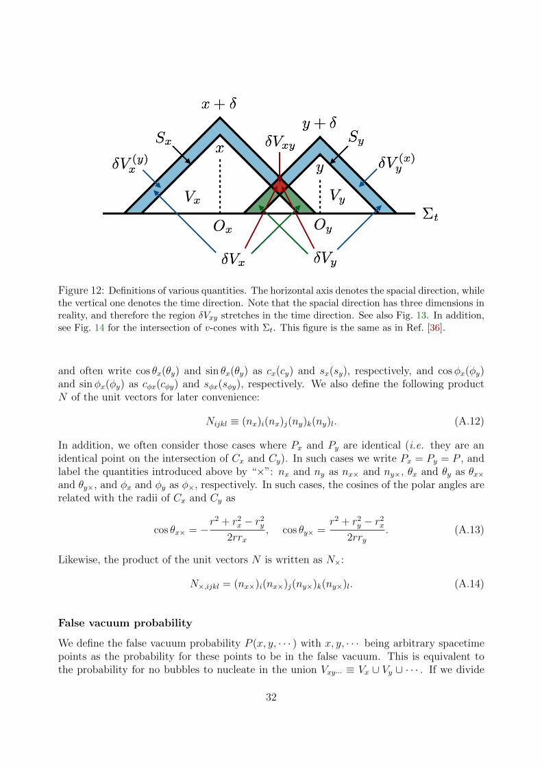
Figure 12: Definitions of various quantities. The horizontal axis denotes the spacial direction, whilethe vertical one denotes the time direction. Note that the spacial direction has three dimensions inreality, and therefore the region δVxy stretches in the time direction. See also Fig. 13. In addition,see Fig. 14 for the intersection of v-cones with Σt. This figure is the same as in Ref. [36].

and often write cos θx(θy) and sin θx(θy) as cx(cy) and sx(sy), respectively, and cosφx(φy)and sinφx(φy) as cφx(cφy) and sφx(sφy), respectively. We also define the following productN of the unit vectors for later convenience:

Nijkl ≡ (nx)i(nx)j(ny)k(ny)l. (A.12)

In addition, we often consider those cases where Px and Py are identical (i.e. they are anidentical point on the intersection of Cx and Cy). In such cases we write Px = Py = P , andlabel the quantities introduced above by “×”: nx and ny as nx× and ny×, θx and θy as θx×and θy×, and φx and φy as φ×, respectively. In such cases, the cosines of the polar angles arerelated with the radii of Cx and Cy as

cos θx× = −r2 + r2

x − r2y

2rrx, cos θy× =

r2 + r2y − r2

x

2rry. (A.13)

Likewise, the product of the unit vectors N is written as N×:

N×,ijkl = (nx×)i(nx×)j(ny×)k(ny×)l. (A.14)

False vacuum probability

We define the false vacuum probability P (x, y, · · · ) with x, y, · · · being arbitrary spacetimepoints as the probability for these points to be in the false vacuum. This is equivalent tothe probability for no bubbles to nucleate in the union Vxy··· ≡ Vx ∪ Vy ∪ · · · . If we divide

32

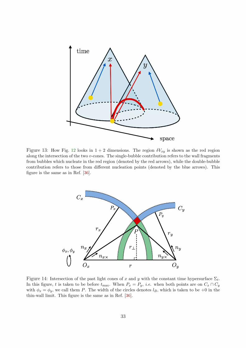
Figure 13: How Fig. 12 looks in 1 + 2 dimensions. The region δVxy is shown as the red regionalong the intersection of the two v-cones. The single-bubble contribution refers to the wall fragmentsfrom bubbles which nucleate in the red region (denoted by the red arrows), while the double-bubblecontribution refers to those from different nucleation points (denoted by the blue arrows). Thisfigure is the same as in Ref. [36].

Figure 14: Intersection of the past light cones of x and y with the constant time hypersurface Σt.In this figure, t is taken to be before tmax. When Px = Py, i.e. when both points are on Cx ∩ Cywith φx = φy, we call them P . The width of the circles denotes lB, which is taken to be +0 in thethin-wall limit. This figure is the same as in Ref. [36].

33

Vxy··· into infinitesimal regions δVi with i being the label for these regions, the probabilitywe need is the product of 1− ΓiδVi over the whole region in Vxy···. Therefore [46],

P (x, y, · · · ) =∏i

(1− ΓidVi) = e−I(x,y,··· ), I(x, y, · · · ) =

∫Vxy···

d4z Γ(tz). (A.15)

Here z = (tz, ~z). Using Eq. (A.15), we can explicitly write down the probability for twospacetime points x and y to remain in the false vacuum. As seen from Fig. 12, the intersectionof the union Vxy with the hypersurface Σt consists of a union of two spheres for t < tmax,while it consists of separate spheres for t > tmax. Therefore, the I function is written as

I(x, y) =

∫ tmax

−∞dt Γ(t)

[π3r3x(2 + cx×)(1− cx×)2 +

π

3r3y(2− cy×)(1 + cy×)2

]+

∫ tx

tmax

dt Γ(t)

[4π

3r3x

]+

∫ ty

tmax

dt Γ(t)

[4π

3r3y

]. (A.16)

Here the quantity in the square parenthesis in the first line is the three-dimensional volumeof the intersection of Vxy with Σt. Note that this expression does not assume any specificform for Γ(t).

For the nucleation rate (2.22), it is straightforward to evaluate the time integration byusing Eqs. (A.9), (A.10) and (A.13). We get♦35

I(x, y) ≡ v3Γ∗et〈x,y〉 I(tx,y, rv), I(tx,y, rv) = 8π

[etx,y/2 + e−tx,y/2 +

t2x,y − (r2v + 4rv)

4rve−rv/2

].

(A.17)

Note that we adopt β = 1 unit without loss of generality.

A.3 Single-bubble spectrum

Conditions for bubble configurations

We now calculate the single-bubble contribution to the GW spectrum (see the red arrowsin Figs. 11 and 13). First let us make clear necessary and sufficient conditions for the wallof a single bubble to contribute to the energy-momentum tensor both at x and y. They aresummarized as

• No bubbles nucleate in Vxy.

• One bubble nucleates in δVxy.

The former condition is understood as follows. If this is not satisfied, some bubble(s) nucleatein Vxy. Such bubbles expand, and the evaluation point ~x or ~y enters these bubbles before theevaluation time tx or ty. Here note that, in the envelope approximation, every spacial pointis passed through by bubble walls only once (see Fig. 1). Therefore there cannot be any wall

♦35 We have changed the definition of I from Ref. [36].

34

fragment at spacetime points x or y. The latter condition is understood as follows. As seenfrom Figs. 12 or 14, those bubbles which contribute to the energy-momentum tensor at x andy must have their nucleation points in δVxy. Though more than one bubbles can nucleatein this region, such a probability is infinitely smaller than the one for a single bubble tonucleate in the thin-wall limit lB → 0. Therefore we have only to take one bubble nucleationinto account.

Expression for GW spectrum

Now let us move on to the calculation of the correlator. First we calculate the probabilitypart. Since the region δVxy exists only before tmax, we limit ourselves to the nucleation timetn < tmax. Let us take a constant-time hypersurface Σtn at time tn. We label “n” to allthe quantities introduced around Eqs. (A.9)–(A.13) to denote that these quantities are onΣtn , like nxn, θxn, φxn, nyn, θyn, φyn and Nn. Denoting by dP (s) (“s” denotes “single”) theprobability for no bubbles to nucleate in Vxy and for one bubble to nucleate in δVxy in thetime interval [tn, tn + dtn] and in the azimuthal angle interval [φn, φn + dφn], we obtain

dP (s) = P (x, y)× r⊥l2B

sin(θxn× − θyn×)dφn × Γ(tn)dtn = P (x, y)× l2B

cyn×

r(s)xn

− cxn×

r(s)yn

dφn × Γ(tn)dtn,

(A.18)

with r(s)xn ≡ rB(tx, tn) and r

(s)yn ≡ rB(ty, tn), and r⊥ = r

(s)xnsxn× = r

(s)yn syn× denotes the distance

from P to the lineOxOy. See Fig. 14. Here the factor r⊥l2Bdφn/ sin(θxn×−θyn×) come from the

infinitesimal three-dimensional volume of the intersection of δVxy with Σtn , i.e. the volumeof the red diamond in Fig. 14 rotated around ~r with an infinitesimal azimuthal angle dφn.The next step is to calculate the value of Tij(x)Tkl(y) when such an event with probabilitydP (s) occurs. From the expression for the energy-momentum tensor (2.16)–(2.17), it is givenby

[Tij(x)Tkl(y)](s) =

(4π

3r(s)3xn κρ0

1

4πr(s)2xn lB

)(4π

3r(s)3yn κρ0

1

4πr(s)2yn lB

)Nn×,ijkl, (A.19)

with Nn×,ijkl being Nn,ijkl when Px and Py are identical: see Eq. (A.14). From these expres-sions, the correlator is obtained by the summation over tn as

〈TijTkl〉(s) (tx, ty, r) =

∫ tn=tmax

tn=−∞dP (s) [Tij(x)Tkl(y)](s) . (A.20)

Now everything is straightforward. Let us first calculate the unequal-time power spectrumΠ(s) in Eq. (2.35), and then the GW spectrum ∆(s) in Eq. (2.41). We can perform theangular integration in Eq. (2.35) with the formula (F.2). In the present case, we substitutethe special value nx× and ny× into nx and ny, and therefore the polar angles are given byEq. (A.13) and φx − φy = φ× − φ× = 0. After integrating out the angular direction of ~r, we

35

obtain

Π(s)(tx, ty, k)

=

∫ ∞v|tx,y |

dr

∫ tmax

−∞dtn

4π2

9κ2ρ2

0

e−I(x,y)Γ(tn)rr(s)2

xn r(s)2yn

×[j0(kr)K0(nxn×, nyn×) +

j1(kr)

krK1(nxn×, nyn×) +

j2(kr)

(kr)2K2(nxn×, nyn×)

] ,(A.21)

where jn are the spherical Bessel functions given in Eqs. (F.6) and the explicit forms ofKn are given in Appendix F. The lower bound of the integration region for r is because theintersection δVxy does not exist for rv ≡ r/v < |tx,y|. Though at this stage we can perform theintegration by tn for the nucleation rate (2.22), we leave it general for a while. Substitutingthis into Eq. (2.41), we obtain the single-bubble spectrum for a general nucleation rate

∆(s) =

∫ ∞−∞

dtx

∫ ∞−∞

dty

∫ ∞v|tx,y |

dr

∫ tmax

−∞dtn

k3

3

e−I(x,y)Γ(tn)rr(s)2

xn r(s)2yn

×[j0(kr)K0(nxn×, nyn×) +

j1(kr)

krK1(nxn×, nyn×) +

j2(kr)

(kr)2K2(nxn×, nyn×)

]cos(ktx,y)

.(A.22)

Here we have substituted tstart, tend = ∓∞.Finally let us consider the nucleation rate (2.22). Given this specific form, we can perform

t〈x,y〉 and tn integrations to obtain the GW spectrum as

∆(s) =

∫ ∞−∞

dtx,y

∫ ∞|tx,y |

drv v3k3 e−

rv2

I(tx,y, rv)

[j0(vkrv)S0 +

j1(vkrv)

vkrvS1 +

j2(vkrv)

(vkrv)2S2

]cos(ktx,y).

(A.23)

Here we have changed the integration variable from r to rv ≡ r/v. Also, Sn functions are

S0 =2

3

(t2x,y − r2v)

2

r3v

(r2v + 6rv + 12),

S1 =2

3

t2x,y − r2v

r3v

[−t2x,y(r3

v + 12r2v + 60rv + 120) + r2

v(r3v + 4r2

v + 12rv + 24)],

S2 =1

6

1

r3v

[t4x,y(r

4v + 20r3

v + 180r2v + 840rv + 1680)

− 2t2x,yr2v(r

4v + 12r3

v + 84r2v + 360rv + 720)

+r4v(r

4v + 4r3

v + 20r2v + 12rv + 24)

], (A.24)

36

and we have used∫∞−∞ dY e

−XeY +nY = (n− 1)!/Xn for t〈x,y〉 integration.

The exponential factor e−rv2 in Eq. (A.23) has a physical origin. For the nucleation rate

(2.22), there is a typical time when spacial points experience the transition from the falseto true vacuum. Fig. 1 roughly corresponds to such a time. This typical transition time isalso a typical time for bubble collisions, as seen from this figure. Let us set the evaluationtimes tx and ty around this typical collision time, because GWs are mainly sourced aroundthis time in the envelope approximation. If we take spacial evaluation points ~x and ~y farseparated with each other, the xy-bubble has to nucleate well before the typical collisiontime. Probabilities for bubble nucleation at such early times are suppressed by e−rv/2, andthis is the origin for the exponential factor in Eq. (A.23).

For the numerical evaluation of Eq. (A.23), see Ref. [36]. It is shown that ∆(s) is propor-tional to k3 for k/β . 1/v, while it behaves as ∝ k−1 for k/β & 1/v.

A.4 Double-bubble spectrum

Conditions for bubble configurations

For the double-bubble spectrum, the procedure is basically the same as the single-bubblecase. The necessary and sufficient conditions for the walls of two different bubbles to con-tribute to the energy-momentum tensor at x and y are summarized as

• No bubbles nucleate in Vxy.

• One bubble nucleates in δV(y)x , and another nucleates in δV

(x)y .

Note that the second condition is different from the single-bubble case. It means that onebubble nucleates in the left blue-shaded region in Fig. 12, and another nucleates in theright blue-shaded region. As mentioned in the beginning of this section, we call the formerand latter bubbles x- and y-bubbles, respectively. Since they nucleate independently ofeach other, we denote the nucleation times for these bubbles by txn and tyn, respectively,and consider constant-time hypersurfaces Σtxn and Σtyn separately when we discuss thenucleation process. We again label all the quantities introduced around Eqs. (A.9)–(A.13)by “n” to denote that these quantities are on these hypersurfaces.

Expression for GW spectrum

Let us consider the probability dP (d) (“d” denotes “double”) where no bubbles nucleate

in δVxy and one bubble nucleates in each of δV(y)x and δV

(x)y in time intervals dtxn and dtyn

within infinitesimal angular intervals dcxndφxn and dcyndφyn, respectively. Such a probabilityis given by

dP (d) = P (x, y)× r(d)2xn lBΓ(txn)dtxndcxndφxn × r(d)2

yn lBΓ(tyn)dtyndcyndφyn. (A.25)

Here we have defined r(d)xn ≡ rB(tx, txn) and r

(d)yn ≡ rB(ty, tyn). The expression (A.25) holds

only for txn < tx and tyn < ty, because otherwise there is no allowed region for bubblenucleation (i.e. the hypersurface Σtxn or Σtyn does not intersect with Vx or Vy). Also, the

37

integration regions for cxn or cyn depend on whether the nucleation time is before or aftertmax. For the former case, the allowed region (the blue-shaded region in Figs. 12 and 14) doesnot form a complete sphere, and therefore the cosines must satisfy cxn > cx× or cyn < cy×.For the latter case, such region forms a complete sphere and cxn or cyn is allowed to takeany value in [−1, 1]. When such an event with probability dP (d) occurs, the expression forthe product of the energy-momentum tensor at the evaluation points x and y becomes

[Tij(x)Tkl(y)](d) =

(4π

3r(d)3xn κρ0

1

4πr(d)2xn lB

)(4π

3r(d)3yn κρ0

1

4πr(d)2yn lB

)Nn,ijkl. (A.26)

Here Nn,ijkl ≡ (nxn)i(nxn)j(nyn)k(nyn)l with nxn and nyn being nx and ny on the constant-time hypersurface Σtxn and Σtyn , respectively. Then, by summing up all the contributionsfrom various nucleation time, we get the following expression for the correlator of the energy-momentum tensor

〈TijTkl〉(d) (tx, ty, r) =

∫ txn=tx

txn=−∞

∫ tyn=ty

tyn=−∞dP (d) [Tij(x)Tkl(y)](d) . (A.27)

Taking Eqs. (A.25) and (A.26) into account, one sees that the integrations with respectto the x bubble and y bubble factorize and therefore can be done separately. SubstitutingEq. (A.27) into Eq. (2.35), and using Eq. (F.2), we have

Π(d)(tx, ty, k) =

∫ ∞v|tx,y |

dr

∫ tmax

−∞dtxn

∫ tmax

−∞dtyn

∫ 1

cxn×

dcxn

∫ cyn×

−1

dcyn

∫ 2π

0

dφxn,yn

4π2

9κ2ρ2

0

e−I(x,y)Γ(txn)Γ(tyn) r2r(d)3

xn r(d)3yn

×[j0(kr)K0(nxn, nyn) +

j1(kr)

krK1(nxn, nyn) +

j2(kr)

(kr)2K2(nxn, nyn)

] .(A.28)

Here φxn,yn ≡ φxn − φyn, and we have integrated out φ〈xn,yn〉 ≡ (φxn + φyn)/2 directionby using Eq. (F.2). Below we explain the integration ranges in this expression. First, thelower bound for the integration region for r comes from the following argument. Under theenvelope approximation, there is no bubble configuration where bubble walls contribute tothe energy-momentum tensor at both x and y if rv < tx,y is satisfied. We illustrate thispoint in Fig. 15. If y is inside the past v-cone of x, the evaluation point ~x is already insidethe y-bubble before the evaluation time tx. In other words, some fragment of the y-bubblehas already passed through ~x before tx. Since any spacial point is passed through by bubblewalls only once in the envelope approximation, there cannot be any wall fragment at ~x attime tx. The same argument holds when x is inside the past v-cone of y, and thereforewe can safely restrict the integration region to rv > tx,y. Second, we explain txn and tynintegrations. We have removed [tmax, tx] and [tmax, ty] from their integration regions (notethat tmax exists because x and y are now taken to be spacelike from the first argument).This is because the contributions from [tmax, tx] and [tmax, ty] vanish because of the sphericalsymmetry. See Fig. 16 for illustration. The removed regions correspond to above the blue-dotted line. Bubbles which nucleate in these regions contribute to the energy-momentum

38

Figure 15: Illustration for why we do not have to take the integration region rv < tx,y intoaccount in the envelope approximation. The horizontal and vertical axes denote the space andtime direction, respectively. For rv < tx,y, the wall of the bubble nucleated on the past v-cone of ypasses through ~x before the evaluation time tx, and hence there can be no bubble wall at ~x at timetx.

tensor at the evaluation points from every direction, and such contributions vanish aftersumming over the whole solid angle. In contrast, for txn and tyn in [−∞, tmax], only limiteddirections are allowed for nucleation for both x- and y-bubbles, as shown in the yellow lines.These allowed directions correspond to the blue-shaded regions in Fig. 14. This explains thelower (upper) bound cxn× (cyn×) for the cxn (cyn) integration.

We can proceed further by integrating out the angular variables. First, note that φxn,ynappears only in K functions. After integrating them out, one sees that only the term pro-portional to the first term in Eq. (F.5) survives. It has a form like (3c2

xn − 1)(3c2yn − 1), and

the variables cxn and cyn appear only in this part. Therefore we can complete the angularintegration and obtain

Π(d)(tx, ty, k)

=

∫ ∞v|tx,y |

dr

∫ tmax

−∞dtxn

∫ tmax

−∞dtyn

16π3

9κ2ρ2

0

e−I(x,y)Γ(txn)Γ(tyn) r2r(d)3

x r(d)3y

×(c3xn× − cxn×)(cyn× − c3

yn×)j2(kr)

(kr)2

.(A.29)

Given this expression, it is straightforward to construct the spectrum ∆(d) by using Eq. (2.41):

∆(d) =

∫ ∞−∞

dtx

∫ ∞−∞

dty

∫ ∞v|tx,y |

dr

∫ tmax

−∞dtxn

∫ tmax

−∞dtyn

4π

3k3

e−I(x,y)Γ(txn)Γ(tyn) r2r(d)3

x r(d)3y

×(c3xn× − cxn×)(cyn× − c3

yn×)j2(kr)

(kr)2cos(ktx,y)

. (A.30)

39

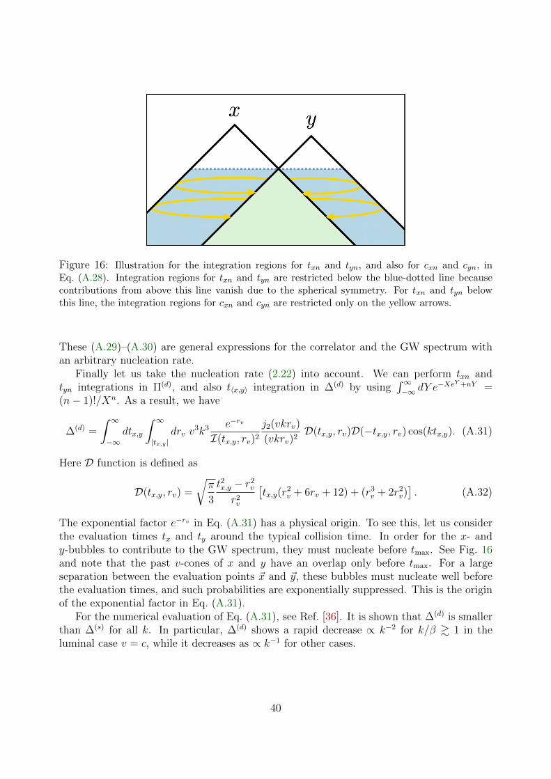
Figure 16: Illustration for the integration regions for txn and tyn, and also for cxn and cyn, inEq. (A.28). Integration regions for txn and tyn are restricted below the blue-dotted line becausecontributions from above this line vanish due to the spherical symmetry. For txn and tyn belowthis line, the integration regions for cxn and cyn are restricted only on the yellow arrows.

These (A.29)–(A.30) are general expressions for the correlator and the GW spectrum withan arbitrary nucleation rate.

Finally let us take the nucleation rate (2.22) into account. We can perform txn andtyn integrations in Π(d), and also t〈x,y〉 integration in ∆(d) by using

∫∞−∞ dY e

−XeY +nY =(n− 1)!/Xn. As a result, we have

∆(d) =

∫ ∞−∞

dtx,y

∫ ∞|tx,y |

drv v3k3 e−rv

I(tx,y, rv)2

j2(vkrv)

(vkrv)2D(tx,y, rv)D(−tx,y, rv) cos(ktx,y). (A.31)

Here D function is defined as

D(tx,y, rv) =

√π

3

t2x,y − r2v

r2v

[tx,y(r

2v + 6rv + 12) + (r3

v + 2r2v)]. (A.32)

The exponential factor e−rv in Eq. (A.31) has a physical origin. To see this, let us considerthe evaluation times tx and ty around the typical collision time. In order for the x- andy-bubbles to contribute to the GW spectrum, they must nucleate before tmax. See Fig. 16and note that the past v-cones of x and y have an overlap only before tmax. For a largeseparation between the evaluation points ~x and ~y, these bubbles must nucleate well beforethe evaluation times, and such probabilities are exponentially suppressed. This is the originof the exponential factor in Eq. (A.31).

For the numerical evaluation of Eq. (A.31), see Ref. [36]. It is shown that ∆(d) is smallerthan ∆(s) for all k. In particular, ∆(d) shows a rapid decrease ∝ k−2 for k/β & 1 in theluminal case v = c, while it decreases as ∝ k−1 for other cases.

40

B GW spectrum beyond the envelope approximation

In this appendix we derive the GW spectrum without the envelope approximation. Thedifference from the envelope case is that the bubble walls now keep their energy and mo-mentum after collision (see Fig. 2). This collision, which we refer to as “interception” in thefollowing, makes the evaluation of 〈T (x)T (y)〉 much more complicated.

B.1 Basic strategy

Basic strategy is the same as in the envelope case. In the present case as well, there are twotypes of contributions:

• Single-bubble

• Double-bubble

The difference appears in the assumption on the functional form of the energy-momentumtensor. It is given by Eq. (2.16), but ρB is now taken to be ρ

(collided)B , where

ρ(collided)B (x) =

[4π

3rB(txi, txn)3κρ0

/4πrB(txi, txn)2lB

]× rB(txi, txn)2

rB(tx, txn)2×D(tx, txi, txn),

= ρ(uncollided)B (x)× rB(txi, txn)3

rB(tx, txn)3×D(tx, txi, txn), (B.1)

for rB(tx, txn) < |~x− ~xn| < r′B(tx, txn), and it vanishes otherwise. Here txi denotes the timewhen the bubble wall fragment is intercepted by some other walls for the first time. Notethat different wall fragments have different txi. The second factor in the R.H.S. of the firstline in Eq. (B.1) takes into account the increase of the bubble-wall area and the resulting lossof the energy and momentum densities after interception. Also, D is a “damping function”,which accounts for how fast collided walls lose their energy and momentum on top of the losscoming from the increase in their area. It depends on the underlying particle model whichdescribes the couplings between the scalar field and light species. Therefore we take D to bearbitrary in the following, except for the condition D(tx, txi = tx, tn) = 1. This is becausethere is no time for damping if the interception occurs at the evaluation time. Note that,in Eq. (B.1), we have assumed that the bubble walls are affected only by the first collisionand not by the subsequent collisions. This is because the energy and momentum in bubblewalls are sourced by the released energy (latent heat) until their first collisions, while thereis no such energy sourcing after that. In Fig. 2, the collided walls, denoted by gray lines,propagate inside other bubbles without energy sourcing after their first collisions.

In the following, we first summarize our notation and then proceed to the calculation of〈T (x)T (y)〉 from single- and double-bubble contributions in turn.

B.2 Prerequisites

Labels for spacetime points

As before, we use x = (tx, ~x) and y = (ty, ~y) for the arguments in 〈T (x)T (y)〉. The bubblewalls which pass through these evaluation points must nucleate somewhere before the evalu-

41

ation times tx and ty. We denote these nucleation points as xn = (txn, ~xn) and yn = (tyn, ~yn),and call these bubbles x- and y-bubbles, respectively. The bubble wall fragments experiencethe interception (the first collision) before the evaluation time in some cases. In such caseswe denote the interception points by xi = (txi, ~xi) and yi = (tyi, ~yi). Note that, as mentionedbefore, the interception times of two wall fragments are generally different even if they belongto the same bubble, and therefore xi and yi depend on the bubble itself and the direction inwhich the fragment is propagating. In summary, our notation is

• n : label for nucleation points

• i : label for interception points

Spacelike theta function

In the following discussion, we often require two spacetime points to be spacelike. We imposethis condition by inserting the spacelike step function Θsp defined by

Θsp(x, y) ≡ Θ(|~x− ~y|2 − (tx − ty)2), (B.2)

to the integrands,♦36 where Θ is the Heaviside theta function.

Shorthand notations

In the calculation below, we often encounter time differences and spacial distances betweentwo spacetime points. Therefore, for brevity, we introduce

tx•,y ≡ tx• − ty, rx•,y ≡ |~x• − ~y|. (B.3)

Also, we define the average as

t〈x•,y〉 ≡tx• + ty

2. (B.4)

In addition, we often take time derivatives along the propagation direction of the wall frag-ment. We write such a derivative of a quantity Q with respect to t• and derivatives withrespect to t• and t as

[Q]t• , [Q]t•,t , (B.5)

and so on. For example, the derivative with respect to txi along the propagation of thex-fragment is written as [Q]txi. The derivatives with respect to txi (along the x-fragment)and tyi (along the y-fragment) is written as [Q]txi,tyi. Note that the order of the derivativeswith respect to t• and t is not important in all the following calculations. We comment onthese derivatives below Eqs. (B.10) and (B.19) with concrete examples.

♦36 There are other ways to impose the spacelike condition, e.g. Θ((|~x− ~y|2 − (tx − ty)2)2). Our results donot depend on how we choose the functional form.

42

Figure 17: Past v-cones relevant in the calculation beyond the envelope. Bubble wall fragmentsare now subject to the interception dynamics, which occurs at the points denoted by the yellowcrosses. For the double-bubble contribution (blue) x and y are not necessarily spacelike, in contrastto the envelope case. On the other hand, for the single-bubble contribution (red), x and y must bespacelike because otherwise the nucleation region δVxy does not exist. See also Fig. 18 for how theleft panel looks in 1 + 2 dimensions.

Figure 18: How the left panel of Fig. 17 looks in 1 + 2 dimensions.

43

B.3 Single-bubble spectrum

Classification

Now we start the calculation of the single-bubble contribution. See Figs. 17 and 18. Notethat x- and y-fragments come from the same nucleation point, and therefore, we can safelylimit ourselves to the spacelike combinations of (x, y). The single-bubble contribution can beclassified into four classes, depending on whether the fragments have already been interceptedor not at the evaluation points:

• CC : Both x and y-fragments have already collided with other bubbles at the evaluationpoints x and y.

• CU : Only x-fragment has already collided with other bubbles and y-fragment remainsuncollided at the evaluation points x and y.

• UC : Only y-fragment has already collided with other bubbles and x-fragment remainsuncollided at the evaluation points x and y.

• UU : Both x and y-fragments remain uncollided at the evaluation points x and y.

In the following, we see that the single-bubble spectrum reduces to a simple expression aftersumming up all these classes.

Simplification formula

In this subsection we introduce a “simplification formula”, which makes the sum of the fourcontributions much simpler.

Let us suppose that the UU contribution to the correlator 〈T (x)T (y)〉 is written as

〈Tij(x)Tkl(y)〉(s,UU) =

∫ tmax

−∞dtn

∫ 2π

0

dφn e−I(x,y)F (s)(x, y;xi = x, yi = y; zn), (B.6)

with some function F (s). We denote the common nucleation point for x and y-fragments byzn = (tn, ~zn), which means xn = yn = zn. Also, φn is the azimuthal angle for the nucleationpoint ~zn with respect to ~r ≡ ~x − ~y. Note that tn and φn completely specify the nucleationpoint zn for given x and y. The explicit expression for F (s) is found in the same way asAppendix A, except that the energy-momentum tensor is now given by Eq. (2.16) with ρBbeing Eq. (B.1):

F (s)(x, y;xi, yi; zn)

=r⊥l

2B

sin(θxn× − θyn×)Γ(tn)

(4π

3r(s)3xn κρ0

1

4πr(s)2xn lB

)(4π

3r(s)3yn κρ0

1

4πr(s)2yn lB

)Nn×,ijkl

× rB(txi, tn)3

r(s)3xn

rB(tyi, tn)3

r(s)3yn

D(tx, txi, tn)D(ty, tyi, tn). (B.7)

44

Here r(s)xn = rB(tx, tn) and r

(s)yn = rB(ty, tn), and r⊥ and Nn×,ijkl are defined in the same way

as Appendix A.3. Note that substituting xi = x and yi = y reproduces the result withthe envelope approximation (A.20). Then, interestingly, the sum of the four contributionsreduces to

〈T (x)T (y)〉(s,UU+UC+CU+CC)

=

∫ tmax

−∞dtn

∫ 2π

0

dφn

∫ tx

txn

dtxi

∫ ty

tyn

dtyi e−I(xi,yi)

[F (s)(x, y;xi, yi, zn)

]txi,tyi

. (B.8)

We prove this formula in Appendix C. Here, the expression [F ]txi,tyi denotes taking thederivatives with respect to txi and tyi along the propagation of the bubble wall fragments,as explained in the previous subsection. In the present case, F (s) in Eq. (B.8) contains theargument xi = (txi, ~xi) and yi = (tyi, ~yi). When taking derivatives with respect to txi and tyi,we regard ~xi and ~yi as functions of them. This is possible once the propagation directionsof x and y-fragments are specified, and in fact they are specified by the variables tn and φn.

Expressions for GW spectrum

Let us derive concrete expressions for Π(s) and ∆(s). First, for a general nucleation rate Γand the damping function D, we obtain the following for Π(s) by using the simplificationformula (B.8):

Π(s)(tx, ty, k) =

∫ ∞v|tx,y |

dr

∫ tmax

−∞dtn

∫ tx

tn

dtxi

∫ ty

tn

dtyi

4π2

9κ2ρ2

0

e−I(xi,yi) Γ(tn)

r

r(s)xnr

(s)yn

×[j0(kr)K0(nxn×, nyn×) +

j1(kr)

krK1(nxn×, nyn×) +

j2(kr)

(kr)2K2(nxn×, nyn×)

]× ∂txi

[rB(txi, tn)3D(tx, txi, tn)

]∂tyi

[rB(tyi, tn)3D(ty, tyi, tn)

]

(B.9)

and the following for ∆(s):

∆(s) =

∫ ∞−∞

dtx

∫ ∞−∞

dty

∫ ∞v|tx,y |

dr

∫ tmax

−∞dtn

∫ tx

tn

dtxi

∫ ty

tn

dtyi

k3

3

e−I(xi,yi) Γ(tn)

r

r(s)xnr

(s)yn

×[j0(kr)K0(nxn×, nyn×) +

j1(kr)

krK1(nxn×, nyn×) +

j2(kr)

(kr)2K2(nxn×, nyn×)

]× ∂txi

[rB(txi, tn)3D(tx, txi, tn)

]∂tyi

[rB(tyi, tn)3D(ty, tyi, tn)

]cos(ktx,y)

.(B.10)

Some comments are in order. First, the r⊥/ sin(θxn×−θyn×) term in Eq. (B.7) has been sim-plified by using the same transformations as around Eq. (A.18). Next, the derivatives with

45

respect to the propagation directions in Eq. (B.8) are now reduced to partial derivatives.This is because txi (tyi) dependence of ~xi (~yi) is encoded in Eq. (B.7) through rB(txi, tn)(rB(tyi, tn)). After reducing the derivatives to partial derivatives, we can perform the inte-gration with respect to φn. Finally, the integration regions are determined as follows. Forr, the lower limit is set because δVxy does not exist for r < v|txy|. See 17 and 18, and alsothe explanation at the beginning of Sec. B.3. The upper limit for tn integration comes fromthe same reason. Also, the integration regions for txi and tyi come from the simplificationformula (B.8).

Here it would be a good exercise to check that these expressions coincide with the expres-sions with the envelope approximation (A.21) and (A.22) if we assume an instant dampingof the wall energy. Such a setup is realized by setting D(t, ti, tn) = Θ(ti − t + ε) with εbeing infinitesimal and positive. With this form, D is unity for time t before ti + ε, while itvanishes after that. The txi and tyi derivatives in Eqs. (B.9) and (B.10) can act both on rBand D, but if either of them acts on rB the integrand vanishes because D is unity only forthe integration range tx−ε < txi < tx or ty−ε < tyi < ty. Therefore these derivatives have toact on D, and this gives δ(txi− tx+ ε) and δ(tyi− ty + ε). Performing txi and tyi integrations,one sees that Eqs. (B.9) and (B.10) coincide with Eqs. (A.21) and (A.22), respectively.

Let us finally derive the expression for ∆(s) with the damping function (2.21) and thenucleation rate (2.22). Given these specific forms we can perform one integration, because wecan shift the whole system in the time direction without changing the geometry of bubbles.In fact, if we write all the time variables in Eq. (B.10) in terms of the difference from thenucleation time tn, all the effects of time shift in the system appears in the exponent I(xi, yi)and the nucleation rate Γ(tn).♦37 Therefore we can integrate out the time shift direction andobtain

∆(s) =

∫ ∞−∞

dtx,y

∫ ∞|tx,y |

drv

∫ ∞rv/2

dt〈x,y〉,n

∫ tx,n

0

dtxi,n

∫ ty,n

0

dtyi,n

v3k3

3

e−(txi,n+tyi,n)/2e−(tx,xi+ty,yi)/τ

I(txi,yi, rxi,yi/v)

(3t2xi,n + t3xi,n/τ)(3t2yi,n + t3yi,n/τ)

tx,nty,n

× rv

[j0(vkrv)K0(nxn×, nyn×) +

j1(vkrv)

vkrvK1(nxn×, nyn×) +

j2(vkrv)

(vkrv)2K2(nxn×, nyn×)

]× cos(k(tx,n − ty,n))

.(B.11)

Note that tx,n, ty,n, tx,xi and ty,yi in this expression should be understood in terms of theintegration variables as

tx,n =tx,y2

+ t〈x,y〉,n, ty,n = −tx,y2

+ t〈x,y〉,n, tx,xi = tx,n − txi,n, ty,yi = ty,n − tyi,n,(B.12)

♦37 In fact, in Eq. (B.10), r(s)xn = vtx,n and r

(s)yn = vty,n contain time differences only, and K functions

contain angular variables such as sxn× and cxn×, which can be written in terms of r, tx,n and ty,n. Also,from rB(txi, tn) = vtxi,n, rB(tyi, tn) = vtyi,n, D(tx, txi, tn) = e−tx,xi/τ and D(ty, tyi, tn) = e−ty,yi/τ , one seesthat the last line also has time differences only.

46

where t〈x,y〉,n = t〈x,y〉− tn. In addition, the arguments txi,yi = txi,n− tyi,n and rxi,yi = |~xi− ~yi|in the I function are also functions of the integration variables. In fact, using the relation~xi − ~yi = ~r + v(tx,xinxn× − ty,yinyn×) (with the subscript n indicating that the vectors nx×and ny× are on the constant-time hypersurface Σtn), one can express rxi,yi as

rxi,yiv

=√r2v + t2x,xi + t2y,yi + 2rvtx,xicxn× − 2rvty,yicyn× − 2tx,xity,yicxyn×, (B.13)

where cxn× and cyn× are the cosines introduced around Eq. (A.13). In addition, cxyn× isthe cosine of the angle between nxn× and nyn× given by cxyn× = cxn×cyn× + sxn×syn×.Alternatively, using ~xi − ~yi = v(−txi,nnxn× + tyi,nnyn×), one has

rxi,yiv

=√t2xi,n + t2yi,n − 2txi,ntyi,ncxyn×, (B.14)

which also gives an expression of rxi,yi in terms of the integration variables.

B.4 Double-bubble spectrum

Classification

Next we move on to the calculation of the double-bubble contribution. We first classifybubble wall properties as in the single-bubble case. The bubble wall fragment reaching theevaluation point x or y is either already collided or still uncollided, as before. In the double-bubble case, however, we need further classification for the former depending on whether thebubble which intercepts the x-(or y-)fragment is the bubble which y-(or x-)fragment belongsto. We illustrate this point in Fig. 19. The horizontal (vertical) axis is the space (time)direction, and the blue arrows denote the propagation of the x- and y-fragments. Note thatthese blue arrows are propagating on the surface of v-cones as in Fig. 18. In the upper-leftpanel, the interception (denoted by the crosses) occurs to the x-(or y-)fragment (denoted byblue arrows) before the wall of the y-(or x-)bubble (denoted by yellow lines) catches up withthe x-(or y-)fragment. In such cases the intercepting bubble is different from the one whichthe other fragment belongs to, and we label such contribution by Ci × Ci. The oppositecase is shown in the lower-right panel, where x-(y-)fragment is intercepted by the bubblewall which the other fragment belongs to. We label such contributions by Cin × Cin. Themeaning of the other two cases Ci × Cin and Cin × Ci is now trivial. Note that whethercontributions including Cin exist or not depends on the choice of the spacetime points x andy and on the choice of the propagation directions.

In summary, we can classify the double-bubble contribution into (U,Ci, Cin)×(U,Ci, Cin),where

• U : x-(or y-)fragment remains uncollided at the evaluation point.

• Ci : x-(or y-)fragment has already been intercepted at the evaluation point, and theinterception occurs with a collision with a bubble other than the y-(or x-)bubble.

• Cin : x-(or y-)fragment has already been intercepted at the evaluation point, and theinterception occurs with a collision with the y-(or x-)bubble.

47

One may notice that Ci×Ci contribution can be classified into two classes: the interceptingbubbles for the x- and y-fragments are identical or not. Both of them can properly be takeninto account by the simplification formula we explain below.

Simplification formula

A simplification formula exists in the double-bubble case as well, which makes the sum of thenine classes (U,Ci, Cin)× (U,Ci, Cin) much simpler. First, let us write the UU contributionin the following form:

〈Tij(x)Tkl(y)〉(d,UU) =

∫ tx

−∞dtxn

∫ ty

−∞dtyn

∫dΩxn

∫dΩyn

Θsp(x, yn)Θsp(xn, y)e−I(x,y)F (d)(x, y;xi = x, yi = y;xn, yn). (B.15)

Here Ωxn and Ωyn denote the propagation directions (θxn, φxn) and (θyn, φyn) of the wallfragments, respectively. Note that the constant-time hypersurfaces at the nucleation timesdiffer for x- and y-bubbles, since the nucleation of x- and y-bubbles occurs independently ofeach other. This argument is the same as Appendix A.4. On the other hand, the integrationranges for these directions are now over the whole solid angle in Eq. (B.15) in contrast to

Appendix A.4. In Appendix A.4 we integrate the nucleation points over δV(y)x = δVx−Vy and

δV(x)y = δVy − Vx, which do not form the whole solid angle. This might seem contradictory,

but actually is not. The spacelike theta functions in Eq. (B.15) guarantee that the integrationranges are effectively the same. We illustrate this point in Fig. 20. The nucleation point xncannot enter the past v-cone of y because Θsp(xn, y) gives zero in such cases, while Θsp(x, yn)guarantees that yn is outside the v-cone of x. Also note that Eq. (B.15) forces (x, y) to bespacelike, because if x and y are timelike the theta functions make the integrand to vanishfor any solid angle. The explicit form of F (d) is read off from the derivation in Appendix A:

F (d)(x, y;xi, yi;xn, yn)

= r(d)2xn lBΓ(txn) r(d)2

yn lBΓ(tyn)

(4π

3r(d)3xn κρ0

1

4πr(d)2xn lB

)(4π

3r(d)3yn κρ0

1

4πr(d)2yn lB

)Nn,ijkl

× rB(txi, txn)3

r(d)3xn

rB(tyi, tyn)3

r(d)3yn

D(tx, txi, txn)D(ty, tyi, tyn). (B.16)

In fact, one sees that the substitution of xi = x and yi = y reproduces Eq. (A.27).Now, the sum of the nine contributions (U,Ci, Cin)× (U,Ci, Cin) gives a simple formula

〈Tij(x)Tkl(y)〉(d,(U,Ci,Cin)×(U,Ci,Cin))

=

∫ tx

−∞dtxn

∫ ty

−∞dtyn

∫ tx

txn

dtxi

∫ ty

tyn

dtyi

∫dΩxn

∫dΩyn

Θsp(xi, yn)Θsp(xn, yi)e−I(xi,yi)

[F (d)(x, y;xi, yi;xn, yn)

]txi,tyi

. (B.17)

Here the subscript on the squared parenthesis denotes the time derivatives along the propa-gation of the wall fragments defined in Appendix B.2. We prove this formula in Appendix C.

48

Figure 19: Illustration for (Ci, Cin) × (Ci, Cin) in the double-bubble contribution. The circlesdenote the nucleation points for the x- and y-fragments, which are shown in blue arrows. Thecrosses on these arrows denote the interception points for these fragments. Note that some choicesof x and y forbid the three types including Cin (i.e. CiCin, CinCi and CinCin). (Top-left) CiCi: theintercepting bubbles for the x- and y-fragments are different from the y- and x-bubbles, respectively.(Top-right) CiCin: the intercepting bubble for the y-fragment is the x-bubble. (Bottom-left) CinCi:the intercepting bubble for the y-fragment is the y-bubble. (Bottom-right) CinCin: the interceptingbubbles for the x- and y-fragments are the y- and x bubbles, respectively.

49

Figure 20: Illustration for the integration ranges for the angular variables in Eq. (B.15). The yellowarrows show how the nucleation point changes as the propagation direction Ωxn (Ωyn) changes ona constant-time hypersurface. For tx > tmax (ty > tmax) the spacelike theta functions in Eq. (B.15)always give unity (the upper two yellow lines), while for tx < tmax (ty < tmax) they make theintegrand vanish if the nucleation point xn (yn) enters the past v-cone of y (x) (the lower twoyellow lines). Also, they always give zero for timelike combinations of x and y. Therefore the

integration ranges are effectively constrained within δV(y)x and δV

(x)y with spacelike combinations

of x and y, and hence Eq. (B.15) is consistent with the calculation in Sec. A.4.

Expressions for GW spectrum

We now derive concrete expressions for Π(d) and ∆(d). For a general nucleation rate Γ andthe dumping function D, the simplification formula (B.17) gives

Π(d)(tx, ty, k) =

∫ ∞0

dr

∫ tx

−∞dtxn

∫ ty

−∞dtyn

∫ tx

txn

dtxi

∫ ty

tyn

dtyi

∫ 1

−1

dcxn

∫ 1

−1

dcyn

∫ 2π

0

dφxn,yn

4π2

9κ2ρ2

0

Θsp(xi, yn)Θsp(xn, yi)e

−I(xi,yi)Γ(txn)Γ(tyn)

× r2

[j0(kr)K0(nxn, nyn) +

j1(kr)

krK1(nxn, nyn) +

j2(kr)

(kr)2K2(nxn, nyn)

]× ∂txi

[rB(txi, txn)3D(tx, txi, txn)

]∂tyi

[rB(tyi, tyn)3D(ty, tyi, tyn)

] ,

(B.18)

50

for the correlator, and

∆(d) =

∫ ∞−∞

dtx

∫ ∞−∞

dty∫ ∞0

dr

∫ tx

−∞dtxn

∫ ty

−∞dtyn

∫ tx

txn

dtxi

∫ ty

tyn

dtyi

∫ 1

−1

dcxn

∫ 1

−1

dcyn

∫ 2π

0

dφxn,yn

k3

3

Θsp(xi, yn)Θsp(xn, yi)e

−I(xi,yi)Γ(txn)Γ(tyn)

× r2

[j0(kr)K0(nxn, nyn) +

j1(kr)

krK1(nxn, nyn) +

j2(kr)

(kr)2K2(nxn, nyn)

]× ∂txi

[rB(txi, txn)3D(tx, txi, tyn)

]∂tyi

[rB(tyi, tyn)3D(ty, tyi, tyn)

]cos(ktx,y)

,(B.19)

for the GW spectrum. Note that the derivatives along the propagation of the wall fragmentshave now reduced to partial derivatives with respect to the interception times txi and tyi,because the dependence of ~xi and ~yi on txi and tyi, respectively, is now encoded in thefunctional form of F (d). Also note that the integration range for r is r > 0 in contrast toAppendix A.4. As explained above, this is because the spacelike theta functions effectivelyguarantee that the nucleation point for the x-(or y-)bubble to be spacelike to the evaluationpoint y (or x). In addition, we have integrated out the azimuthal angle (φxn+φyn)/2 becausethe geometry of the system is independent of this direction. This leaves φxn,yn = φxn − φynas the only remaining azimuthal angle.

Again it would be a good exercise to check that Eqs. (B.18) and (B.19) coincide withthe expressions with the envelope approximation (A.29) and (A.30) if we assume an instantdamping of the wall energy. As in Sec. B.3, we take the damping function to be D(t, ti, tn) =Θ(ti − t + ε) with ε being infinitesimal and positive. The txi and tyi derivatives have to acton the damping functions due to the same reason as the previous subsection, and we cancomplete txi and tyi integrations using the resulting delta functions. Now the spacelike thetafunctions are replaced by Θsp(x, yn) and Θsp(y, xn), and hence only spacelike combinationsof (x, yn) and (y, xn) are allowed. Since the integration tx > tmax or ty > tmax gives vanishingcontributions due to the spherical symmetry, one can safely restrict the integration range totx < tmax and ty < tmax to obtain Eq. (A.28). The same arguments as Appendix A.4 lead toEqs. (A.29) and (A.30).

Finally we derive the GW spectrum with the nucleation rate (2.22) and the dampingfunction (2.21). Given these specific forms, we can perform the integration with respectto the overall time shift of the system. In fact, one can write all the time variables inEq. (B.19) in terms of time differences except for the exponent I(xi, yi) and the nucleationrate Γ(txn)Γ(tyn). From the derivation in Appendix A.4 we know that such a time shift

51

direction can be integrated out. As a result, we have ♦38

∆(d) =

∫ ∞−∞

dtx,y

∫ ∞0

drv∫ ∞0

dtx,xn

∫ ∞0

dty,yn

∫ tx,xn

0

dtx,xi

∫ ty,yn

0

dty,yi

∫ 1

−1

dcxn

∫ 1

−1

dcyn

∫ 2π

0

dφxn,yn

v3k3

3

Θsp(xi, yn)Θsp(xn, yi)

× e−(txi,xn+tyi,yn)e−(tx,xi+ty,yi)/τ

I(txi,yi, rxi,yi/v)2(3t2xi,xn + t3xi,xn/τ)(3t2yi,yn + t3yi,yn/τ)

× r2v

[j0(vkrv)K0(nxn, nyn) +

j1(vkrv)

vkrvK1(nxn, nyn) +

j2(vkrv)

(vkrv)2K2(nxn, nyn)

]× cos(ktx,y)

.

(B.20)

Note that time differences such as txi,xn, tyi,yn and txi,yi are expressed in terms of the inte-gration variables as txi,xn = tx,xn− tx,xi, tyi,yn = ty,yn− ty,yi, and txi,yi = tx,y − tx,xi + ty,yi. Inaddition, rxi,yi = |~xi − ~yi| can also be written in terms of the integration variables. In fact,the relation ~xi − ~yi = ~r + v(tx,xinxn − ty,yinyn) gives

rxi,yiv

=√r2v + t2x,xi + t2y,yi + 2rvtx,xicxn − 2rvty,yicyn − 2tx,xity,yicxyn, (B.21)

where cxyn is the cosine of the angle between nxn and nyn given by cxyn = cxncyn +sxnsyn cos(φxn − φyn).

♦38 In Eq. (B.19), the spacelike theta functions as well as the second and third lines in the squareparenthesis contain time differences only. Therefore, overall time-shift dependence appears only inI(xi, yi) = v3Γ∗e

t〈x,y〉/2e−(tx,xi+ty,yi−rxi,yi/v)/2I(txi,yi, rxi,yi) and the nucleation rate Γ(txn)Γ(tyn) =Γ2∗e

2t〈x,y〉e−(tx,xn+ty,yn), in the form of et〈x,y〉 . After rewriting tx and ty integrations into t〈x,y〉 and tx,yintegrations, and expressing all the other time integration variables in terms of time differences like tx,xn,ty,yn, tx,xi and ty,yi, we can integrate out t〈x,y〉 direction to obtain Eq. (B.20).

52

C Derivation of the simplification formulas

In this appendix we derive the simplification formulas (B.8) and (B.17).

C.1 Single-bubble simplification formula

Let us start from Eq. (B.6), which is written here again for completeness

〈Tij(x)Tkl(y)〉(s,UU) =

∫ tmax

−∞dtn

∫dφn e

−I(x,y)F (s)(x, y;xi = x, yi = y; zn), (C.1)

and show that other contributions are written as

〈T (x)T (y)〉(s,UC) =

∫ tmax

−∞dtn

∫dφn

∫ ty

tyn

dtyi [I(x, yi)]tyi e−I(x,yi)F (s)(x, y;xi = x, yi; zn),

〈T (x)T (y)〉(s,CU) =

∫ tmax

−∞dtn

∫dφn

∫ tx

txn

dtxi [I(xi, y)]txi e−I(xi,y)F (s)(x, y;xi, yi = y; zn),

〈T (x)T (y)〉(s,CC) =

∫ tmax

−∞dtn

∫dφn

∫ tx

txn

dtxi

∫ ty

tyn

dtyi[[I(xi, yi)]txi [I(xi, yi)]tyi − [I(xi, yi)]txi,tyi

]e−I(xi,yi)F (s)(x, y;xi, yi, zn),

(C.2)

where remember that the subscripts on the square bracket mean taking the derivative withrespect to that quantity along the propagation of the bubble wall fragments.

In deriving the simplification formula, it would be instructive to see the structure ofEq. (C.1). It consists of two parts. One is P (x, y) = e−I(x,y), which guarantees that nobubbles nucleate in Vx ∪ Vy. This is necessary because otherwise at least one of the x- andy-fragments collides before the evaluation time with bubble(s) which nucleate in Vx ∪ Vy.The other is F (s), which takes into account the probability for nucleation of the xy-bubble(with the infinitesimal time intervals dtn and angle dφn) and the resulting values of theenergy-momentum tensor at the evaluation points.

Let us see how these arguments change in other contributions, taking CU as an example.See the left panel of Fig. 21. We first consider the change in the false vacuum probability.Since now the x-fragment is allowed to collide with other bubbles after it is intercepted atxi (i.e., in the left panel of Fig. 21, bubble walls are allowed to cross the left red arrow atanywhere from xi to x), we do not require that no bubbles nucleate in Vx ∪ Vy. Instead, werequire that the x-fragment remain uncollided until it reaches xi:

• No bubbles nucleate in the union of past v-cones of xi and y.

However, this condition does not guarantee that the x-fragment is intercepted at xi. Let usassume that the x-fragment is intercepted between the infinitesimal time interval [txi, txi +dtxi], and let us consider where such an intercepting bubble can nucleate. Since we are nowfocusing on C“U” contribution, we require the following for such a bubble:

53

• The bubble which intercepts the x-fragment nucleates somewhere on the past v-coneof xi, and it does not intercept the y-fragment before the evaluation time ty.

The nucleation region satisfying this requirement is shown as the yellow band in the leftpanel of Fig. 21. Here xi + δxi is the spacetime point of the x-fragment at time tx + dtx.

The probability for both of the two events above to occur is given by P (xi + δxi, y) −P (xi, y) = [I(xi, y)]txi e

−I(xi,y)dtxi. The reason is simple: if there is any difference betweenthe false vacuum probabilities P (xi + δxi, y) and P (xi, y), the difference corresponds to theprobability for a transition from the false to the true vacuum occurs somewhere betweenxi and xi + δxi. This transition means that a fragment propagating from xi and xi + δxiis intercepted by a bubble which nucleates somewhere in the yellow band in the left panelof Fig. 21 (i.e. Vxi+δxi − (Vxi ∪ Vy)). Note that we do not have to care about how manyintercepting bubbles nucleate, because in the thin-wall limit the number of such bubblesreduces to unity. Another way to understand this expression is to note that [I(xi, y)]txi dtxi =I(xi + δxi, y)− I(xi, y) gives the integration of the nucleation probability Γ over the yellowband, which gives the probability for a single bubble nucleation in this region in the thin-walllimit, while e−I(xi,y) guarantees that no bubbles nucleate in Vxi ∪ Vy.

Now, the replacement for F (s) is easy to find. The only change is in the value of theenergy-momentum tensor due to the fact that the x-fragment cannot be sourced after theinterception at xi. Therefore we use F (s)(x, y;xi, yi = y; zn) instead of F (s)(x, y;xi = x, yif =y; zn). Taking all the above into account, and integrating with the interception time, onehas the CU contribution in Eq. (C.2). The UC contribution is given by the same argumentwith the roles of x• and y• interchanged.

Lastly, let us consider the CC contribution. See the lower panel of Fig. 21. Supposethat the interceptions occur in the time intervals [tx, tx + dtx] and [ty, ty + dty] for the x- andy-fragments, respectively. There are two cases for this:

• One bubble nucleates in Vxi+δxi−(Vxi∪Vyi+δyi) (the left yellow band in the lower panelof Fig. 21), and another nucleates in Vyi+δyi − (Vxi+δxi ∪ Vyi) (the right yellow band inthe same figure).

• One bubble nucleates in the small spacetime region (Vxi+δxi ∪ Vyi+δyi − Vxi ∪ Vyi) −(Vxi+δxi − Vxi)− (Vyi+δyi − Vyi) (the small yellow diamond in the same figure).

The former means that the two intercepting bubbles are different, while in the latter a singlebubble intercepts both the x- and y-fragments. Under the condition that no bubbles nucleatein Vxi∪Vyi (which occurs with probability e−I(xi,yi)), the probability for the former is given by[I(xi, yi)]txi [I(xi, yi)]tyi dtxidtyi, while that for the latter is given by − [I(xi, yi)]txi,tyi dtxidtyi.

For the F (s) function, we have only to use F (s)(x, y;xi, yi; zn). Therefore we obtain theexpression in Eq. (C.2).

Once we have Eqs. (C.1) and (C.2), their sum becomes much simpler. Noting thatF (s)(x, y;xi = xn, yi; zn) and F (s)(x, y;xi, yi = yn; zn) vanish because those bubbles inter-

54

cepted just after nucleation have vanishing energy and momentum, we obtain

〈T (x)T (y)〉(s,UU+UC+CU+CC)

=

∫ tmax

−∞dtn

∫dφn

∫ tx

txn

dtxi

∫ ty

tyn

dtyi e−I(xi,yi)

[F (s)(x, y;xi, yi, zn)

]txi,tyi

, (C.3)

after integration by parts. This is what we call the “simplification formula” for the single-bubble.

Figure 21: (Top-left) CU contribution. The x-fragment is intercepted in the time interval [tx, tx +dtx] by some bubble which does not intercept the y-fragment before ty. Such a bubble nucleatesin the thin yellow band. Note that the red arrows are on the past v-cones of x and y, and theirinclinations do not mean that bubble walls propagate slower than v: see Fig. 13. (Top-right) UCcontribution. Same as the top-left, except that the roles of x and y are interchanged. (Bottom) CCcontribution. This contains two cases: one is that one bubble nucleates in each of the left and rightthin yellow bands, and the other is that only one bubble nucleates in the small yellow diamond inthe center.

55

C.2 Double-bubble simplification formula

(U,Ci)× (U,Ci) contributions

Let us start from Eq. (B.6), which is written here again for completeness

〈Tij(x)Tkl(y)〉(d,UU) =

∫ tx

−∞dtxn

∫ ty

−∞dtyn

∫dΩxn

∫dΩyn

Θsp(x, yn)Θsp(xn, y)e−I(x,y)F (d)(x, y;xi = x, yi = y;xn, yn). (C.4)

Below we first show that the other contributions in (U,Ci)× (U,Ci) are expressed as

〈Tij(x)Tkl(y)〉(d,UCi) =

∫ tx

−∞dtxn

∫ ty

−∞dtyn

∫ ty

tyn

dtyi

∫dΩxn

∫dΩyn

Θsp(x, yn)Θsp(xn, yi) [I(x, yi)]tyi e−I(x,yi)F (d)(x, y;xi = x, yi;xn, yn),

〈Tij(x)Tkl(y)〉(d,CiU) =

∫ tx

−∞dtxn

∫ ty

−∞dtyn

∫ tx

txn

dtxi

∫dΩxn

∫dΩyn

Θsp(xi, yn)Θsp(xn, y) [I(xi, y)]txi e−I(xi,y)F (d)(x, y;xi, yi = y;xn, yn),

〈Tij(x)Tkl(y)〉(d,CiCi) =

∫ tx

−∞dtxn

∫ ty

−∞dtyn

∫ tx

txn

dtxi

∫ ty

tyn

dtyi

∫dΩxn

∫dΩyn

Θsp(xi, yn)Θsp(xn, yi)[[I(xi, yi)]txi [I(xi, yi)]tyi − [I(xi, yi)]txi,tyi

]e−I(xi,yi)F (d)(x, y;xi, yi;xn, yn). (C.5)

Let us remember the arguments in Appendix B when we derive Eq. (C.4). The spaceliketheta functions require (x, yn) and (xn, y) to be spacelike. This is because, for timelike (x, yn)for example, either of the following two occurs:

• For tx < tyn, yn is in the future v-cone of x and therefore ~yn is already inside thex-bubble at the nucleation time tyn. This makes the nucleation of the y-bubble impos-sible.

• For tx > tyn, x is in the future v-cone of yn and therefore ~x is already inside they-bubble at the evaluation time tx. This is not “U” type contribution.

Therefore, the spacelike theta functions select out proper combinations of the nucleationpoints xn and yn for given x and y. Also, the false vacuum probability P (x, y) = e−I(x,y)

guarantees that no bubbles nucleate in Vx ∪ Vy, while the probability for bubble nucleationat proper spacetime points and the value of the energy-momentum tensor at the evaluationpoints are encoded in F (d).

These arguments are modified in the other contributions in (U,Ci)× (U,Ci). Let us takeCiU as an example. See the left panel of Fig. 22. Now the x-fragment has already beenintercepted at the evaluation point tx, and therefore, in contrast to UU contribution, aaa wedo not have to guarantee the “U”(uncollided)-ness of the x-fragment by Θsp(x, yn). Instead,Θsp(x, yn) must be replaced with Θsp(xi, yn). The reason is as follows. Even though the

56

x-fragment is allowed to collide with other bubbles before the evaluation time tx, it is notallowed before txi because xi is the interception point, or the first collision point, by definition.Therefore we have to guarantee the “U”-ness of the x-fragment until the interception pointxi, and that is why we replace Θsp(x, yn) with Θsp(xi, yn).♦39 On the other hand, the otherspacelike theta function Θsp(xn, y) remains the same, because otherwise the “U”-ness of they-fragment is not guaranteed. The derivation of the remaining part (i.e. [I(x, yi)]tyi e

−I(x,yi)

and F (d)) is basically the same as the single-bubble simplification formula. Since the spaceliketheta functions themselves do not guarantee that proper bubble configurations are realized,we have to impose the following in order to realize such bubble configurations:

• No bubbles nucleate in the union of the past v-cones of xi and y.

• The bubble which intercepts the x-fragment nucleates somewhere on the past v-coneof xi, and it does not intercept the y-fragment before the evaluation time ty.

Just as the single-bubble simplification formula, these are simultaneously taken into accountby considering P (xi + δxi, y) − P (xi, y) = [I(xi, y)]txi e

−I(xi,y) for the interception of thex-fragment in the time interval [txi, txi + dtxi]. For the F (d) function, we have only touse F (d)(x, y;xi = x, yi;xn, yn) to replace the value of the energy-momentum tensor at theevaluation points. These considerations give the expression for CiU in Eq. (C.5). For theUCi contribution, the same argument holds with the roles of x• and y• interchanged.

For the CiCi contributions there are two possibilities, just like CC in the single-bubblecontribution (see the bottom panel of Fig. 22):

• One bubble nucleates in Vxi+δxi − (Vxi ∪ Vyi+δyi), and another nucleates in Vyi+δyi −(Vxi+xi+δxi ∪ Vyi).

• One bubble nucleates in the small spacetime region (Vxi+δxi ∪ Vyi+δyi − Vxi ∪ Vyi) −(Vxi+δxi − Vxi)− (Vyi+δyi − Vyi).

The sum of these two probabilities gives[[I(xi, yi)]txi [I(xi, yi)]tyi − [I(xi, yi)]txi,tyi

]dtxidtyi.

For the F (d) function, we use F (d)(x, y;xi, yi;xn, yn) to take both interceptions into account.This completes the proof of Eq. (C.5). Now, using integration by parts as in derivingEq. (C.3), we have

〈Tij(x)Tkl(y)〉(d,UU+UCi+CiU+CiCi)

=

∫ tx

−∞dtxn

∫ ty

−∞dtyn

∫ tx

txn

dtxi

∫ ty

tyn

dtyi

∫dΩxn

∫dΩyn

e−I(xi,yi)[Θsp(xi, yn)Θsp(xn, yi)F (d)(x, y;xi, yi;xn, yn)

]txi,tyi

, (C.6)

♦39 After this replacement, x and yn are no longer spacelike. One might worry that, if x and yn are timelikewith tx < tyn, nucleation of the y-bubble is not guaranteed because yn is inside the future v-cone of x,which is inside the future v-cone of xn (that is, ~yn has already been past by the x-bubble at the nucleationtime tyn). However, this never occurs. If yn is inside the future v-cone of x, it means that yn is also insidethe future v-cone of xi because the latter v-cone contains the former. Such a combination of xi and yn isforbidden by Θsp(xi, yn).

57

as the sum of the four contributions.Below we see the behavior of the time derivatives acting on the spacelike theta functions

in Eq. (C.6), because such terms partly cancel out with the other five contributions in(U,Ci, Cin) × (U,Ci, Cin). In the following, for given x and y, we regard Eq. (C.6) as firstfixing (txn, tyn) and (Ωxn,Ωyn) and then scanning (txi, tyi), which means that we scan (xi, yi)along the propagation lines of x- and y-fragments. Now, let us consider [Θsp(xi, yn)]txi forexample. From the definition of the subscript on the square bracket, we take the derivativeby changing txi in Θsp(xi, yn) along the propagation of the x-fragment. This derivative isnonzero only when the spacetime relation between (xi, yn) changes from timelike to spacelike(Θsp changes from 0 to 1) or spacelike to timelike (Θsp changes from 1 to 0). Such a spacetimepoint is either

• On the past v-cone of yn.

• On the future v-cone of yn.

We denote these points by x(past)in and x

(future)in , respectively. See Fig. 23 for illustration.

Though in this figure both x(past)in and x

(future)in seem to exist, this is an artifact arising from

plotting in two-dimensions. In fact, after some consideration, one sees that there is only onesuch point along the propagation line of the x-fragment for given evaluation points (x, y)and propagation directions (Ωxn,Ωyn).♦40♦41 After further consideration, one sees that onlythe future crossing point can appear in the integration region for txi, and the past crossingpoint never appears in the integration.♦42 Therefore we write x

(future)in simply as xin, and

♦40 In fact, the spacetime crossing point between the propagation line of the x-fragment and both thepast and future v-cones of yn can be calculated by squaring the identity ~xin − ~yn = (~xin − ~x) − (~yn − ~x)with |~xin − ~yn| = v|txin,yn|, ~xin − ~x = −vtx,xinnx and ~yn − ~x = −~r + vty,ynny. Also, the crossing pointbetween the propagation line of the y-fragment and the past and future v-cones of xn is obtained by squaring~yin − ~xn = (~yin − ~y)− (~xn − ~y) with |~yin − ~xn| = v|tyin,xn|, ~yin − ~y = −vty,yinny and ~xn − ~y = ~r+ vtxn,xnx.The resulting expressions are

txin,x =−t2x,yn + t2y,yn + r2 − 2ty,ynrcy

2(tx,yn + rcx − ty,yncxy), tyin,y =

−t2y,xn + t2x,xn + r2 + 2tx,xnrcx

2(ty,xn − rcy − tx,xncxy). (C.7)

Here cxy = nx · ny is the cosine between the propagation angles of x- and y-fragments, and also we havepresented these crossing points in terms of time differences txin,x = txin − tx and tyin,y = tyin − ty. Thismeans that there is a unique spacetime crossing point between the propagation line and the v-cones.♦41 For special propagation directions with which the denominator of txin,x or tyin,y in Eq. (C.7) vanishes,

there is no spacetime crossing between the propagation line and the v-cone. Also, if the numerator vanishesin addition, there are infinite number of the crossing points. However, since such contributions occupy avanishing measure in the integration, we can safely neglect them.♦42 The past crossing point does not appear in the integration region for the following reason. Suppose

that it appears. Then, denoting the past crossing point by xin for brevity, one finds that

(xn, xin) is null with txn < txin.

Also one finds that

(xin, yn) is null with txin < tyn, (yn, yi) is null with tyn < tyi.

Spacetime points xn and yi satisfying these three conditions are timelike (except for limited cases withvanishing integration measure). Therefore the other spacelike theta function Θsp(xn, yi) in Eq. (C.6) vanishes.

58

take only this into account. The future crossing point between the propagation line of they-fragment and the v-cones of xn is defined in the same way, and we call it yin. Now thetime derivatives give

[Θsp(xi, yn)]txi = −δ(txi − txin), [Θsp(xn, yi)]tyi = −δ(tyi − tyin), (C.8)

where the minus signs arise because Θsp changes from 1 to 0 at the future crossing points.Therefore, we can rewrite Eq. (C.6) as

〈Tij(x)Tkl(y)〉(d,UU+UCi+CiU+CiCi)

=

∫ tx

−∞dtxn

∫ ty

−∞dtyn

∫ tx

txn

dtxi

∫ ty

tyn

dtyi

∫dΩxn

∫dΩyn

e−I(xi,yi)

δ(txi − txin)δ(tyi − tyin)F (d)(x, y;xi, yi, xn, yn)

− δ(txi − txin)Θsp(xn, yi)[F (d)(x, y;xi, yi, xn, yn)

]tyi

− Θsp(xi, yn)δ(tyi − tyin)[F (d)(x, y;xi, yi, xn, yn)

]txi

+ Θsp(xi, yn)Θsp(xn, yi)[F (d)(x, y;xi, yi, xn, yn)

]txi,tyi

. (C.9)

Below we see some of these terms cancel out with the other five contributions to give a simpleformula.

(U,Ci, Cin)× (U,Ci, Cin) contributions

Let us see the other five contributions, UCin, CinU , CiCin, CinCi and CinCin. Rememberthat Cin refers to those contributions where the x-(or y-)fragment is intercepted by the y-(orx-)bubble. Therefore, whether such a contribution exists or not depends on whether thefuture crossing point txin or tyin lies in the integration region [txn, tx] or [tyn, ty], respectively.However, in any cases, the five contributions can be written as follows:

〈Tij(x)Tkl(y)〉(d,UCin) =

∫ tx

−∞dtxn

∫ ty

−∞dtyn

∫ ty

tyn

dtyi

∫dΩxn

∫dΩyn

Θsp(x, yn)δ(tyi − tyin)e−I(x,yi)F (d)(x, y;x, yi;xn, yn), (C.10)

〈Tij(x)Tkl(y)〉(d,CinU) =

∫ tx

−∞dtxn

∫ ty

−∞dtyn

∫ tx

txn

dtxi

∫dΩxn

∫dΩyn

δ(txi − txin)Θsp(xn, y)e−I(xi,y)F (d)(x, y;xi, y;xn, yn), (C.11)

〈Tij(x)Tkl(y)〉(d,CiCin) =

∫ tx

−∞dtxn

∫ ty

−∞dtyn

∫ tx

txn

dtxi

∫ ty

tyn

dtyi

∫dΩxn

∫dΩyn

Θsp(xi, yn)δ(tyi − tyin) [I(xi, yi)]txi e−I(xi,yi)F (d)(x, y;xi, yi;xn, yn),

(C.12)

59

Figure 22: (Top-left) CiU contribution. The x-fragment is intercepted in the time interval [tx, tx+dtx] by some bubble which do not intercept the y-fragment before ty. (Top-right) UCi contribution.Same as the left panel, except that the role of x and y are interchanged. (Bottom) CiCi contribution.One possibility is that one bubble nucleates in each of the left and right thin yellow region, andthe other possibility is that only one bubble nucleates in the small diamond-shaped region.

60

Figure 23: Definition of x(past)in , x

(future)in (left) and y

(past)in , y

(future)in (right). They are the spacetime

crossing points of the propagation line of the x-(y-)fragment and the v-cones of yn (xn). If thecrossing point is on the past (future) v-cone, we label it with past (future). The derivative of thespacelike theta function [Θsp(xi, yn)]txi or [Θsp(xn, yi)]tyi is nonzero only at these points. Note that

there is only either of x(past)in or x

(future)in (y

(past)in or y

(future)in ). See the main text on this point.

〈Tij(x)Tkl(y)〉(d,CinCi) =

∫ tx

−∞dtxn

∫ ty

−∞dtyn

∫ tx

txn

dtxi

∫ ty

tyn

dtyi

∫dΩxn

∫dΩyn

δ(txi − txin)Θsp(xn, yi) [I(xi, yi)]tyi e−I(xi,yi)F (d)(x, y;xi, yi;xn, yn),

(C.13)

〈Tij(x)Tkl(y)〉(d,CinCin) =

∫ tx

−∞dtxn

∫ ty

−∞dtyn

∫ tx

txn

dtxi

∫ ty

tyn

dtyi

∫dΩxn

∫dΩyn

δ(txi − txin)δ(tyi − tyin)e−I(xi,yi)F (d)(x, y;xi, yi;xn, yn). (C.14)

First let us see the CinU contribution (C.11). When the future crossing point txin does notlie in the integration region [txn, tx], this expression trivially holds since it vanishes. Onthe other hand, when txin lies in the integration region [txn, tx], one can perform the txiintegration. This replaces all the xi in the integrand with xin. Now the meanings of thefactors in the integrand are clear: Θsp(xn, y) guarantees the “U”-ness of the y-fragment.P (xin, y) = e−I(xin,y) guarantees that no bubbles nucleate in the union of the past v-cones ofxin and y, which is necessary for xin to be the interception (first collision) point and for yto remain uncollided until the evaluation time. F (d) with xi replaced by xin represents theproper value of the energy-momentum tensor. Note that no spacelike theta function appearsfor xi and yn because they are null with each other in the present case. The same argumentsapply to UCin contribution (C.10).

Next let us see the CinCi contribution (C.13). This trivially holds when txin does notlie in the integration region [txn, tx]. In the opposite case, one can perform txi integrationto replace all the xi in the integrand with xin. Now the meanings of the factors in theintegrand are as follows: Θsp(xn, yi) guarantees that yi is the interception (first collision)

61

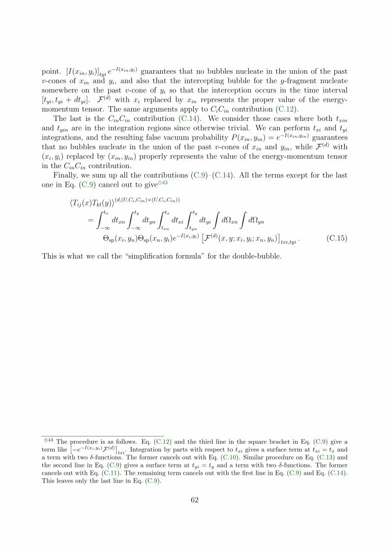
point. [I(xin, yi)]tyi e−I(xin,yi) guarantees that no bubbles nucleate in the union of the past

v-cones of xin and yi, and also that the intercepting bubble for the y-fragment nucleatesomewhere on the past v-cone of yi so that the interception occurs in the time interval[tyi, tyi + dtyi]. F (d) with xi replaced by xin represents the proper value of the energy-momentum tensor. The same arguments apply to CiCin contribution (C.12).

The last is the CinCin contribution (C.14). We consider those cases where both txinand tyin are in the integration regions since otherwise trivial. We can perform txi and tyiintegrations, and the resulting false vacuum probability P (xin, yin) = e−I(xin,yin) guaranteesthat no bubbles nucleate in the union of the past v-cones of xin and yin, while F (d) with(xi, yi) replaced by (xin, yin) properly represents the value of the energy-momentum tensorin the CinCin contribution.

Finally, we sum up all the contributions (C.9)–(C.14). All the terms except for the lastone in Eq. (C.9) cancel out to give♦43

〈Tij(x)Tkl(y)〉(d,(U,Ci,Cin)×(U,Ci,Cin))

=

∫ tx

−∞dtxn

∫ ty

−∞dtyn

∫ tx

txn

dtxi

∫ ty

tyn

dtyi

∫dΩxn

∫dΩyn

Θsp(xi, yn)Θsp(xn, yi)e−I(xi,yi)

[F (d)(x, y;xi, yi;xn, yn)

]txi,tyi

. (C.15)

This is what we call the “simplification formula” for the double-bubble.

♦43 The procedure is as follows. Eq. (C.12) and the third line in the square bracket in Eq. (C.9) give aterm like

[−e−I(xi,yi)F (d)

]txi

. Integration by parts with respect to txi gives a surface term at txi = tx anda term with two δ-functions. The former cancels out with Eq. (C.10). Similar procedure on Eq. (C.13) andthe second line in Eq. (C.9) gives a surface term at tyi = ty and a term with two δ-functions. The formercancels out with Eq. (C.11). The remaining term cancels out with the first line in Eq. (C.9) and Eq. (C.14).This leaves only the last line in Eq. (C.9).

62

D Techniques for numerical evaluation

In this appendix we explain several techniques in evaluating the GW spectrum.

D.1 Equivalent ways to impose the spacelike conditions

In the double-bubble contribution (B.20), we encounter two spacelike theta functions. Inthis subsection, we show that they can be replaced by one spacelike theta function. Thisreplacement makes it possible to integrate out tx,xn and ty,yn directions, and as a result leavesseven-dimensional integration.

First, we write Eq. (B.20) here again for completeness:

∆(d) =

∫ ∞−∞

dtx,y

∫ ∞0

drv∫ ∞0

dtx,xn

∫ ∞0

dty,yn

∫ tx,xn

0

dtx,xi

∫ ty,yn

0

dty,yi

∫ 1

−1

dcxn

∫ 1

−1

dcyn

∫ 2π

0

dφxn,yn

v3k3

3

Θsp(xi, yn)Θsp(xn, yi)

× e−(txi,xn+tyi,yn)e−(tx,xi+ty,yi)/τ

I(txi,yi, rxi,yi/v)2(3t2xi,xn + t3xi,xn/τ)(3t2yi,yn + t3yi,yn/τ)

× r2v

[j0(vkrv)K0(nxn, nyn) +

j1(vkrv)

vkrvK1(nxn, nyn) +

j2(vkrv)

(vkrv)2K2(nxn, nyn)

]× cos(ktx,y)

.

(D.1)

Suppose that we first fix the evaluation points (x, y) and the propagation directions of thewall fragments (Ωxn,Ωyn). Then, the spacelike theta functions in this expression require twonucleation points (xn, yn) and two interception points (xi, yi) to satisfy

• (xi, yn) are spacelike.

• (xn, yi) are spacelike.

We illustrate this procedure in the left panel of Fig. 24. Fixing (x, y) and (Ωxn,Ωyn) cor-responds to fixing the separation and directions of the two blue lines in this figure. Thenfinding (xn, yn) and (xi, yi) satisfying the above conditions means finding four points on theselines so that (xi, yn) and (xn, yi) are spacelike (denoted by the green solid lines). Now weargue that this procedure is equivalent to the following

• Find spacelike (xi, yi).

• Fix (xn, yn) so that xn lies between xni and xi and yn lies between yni and yi.

Here xni and yni are defined as the spacetime crossing points between the propagation linesof the x- and y-fragments and the past v-cone of yi and xi, respectively. We illustrate thisprocedure in the right panel of Fig. 24.

63

Figure 24: Two equivalent ways of imposing the spacelike conditions. Spacelike points are con-nected with green lines. (Left) Fix the four points so that (xi, yn) and (xn, yi) are spacelike. (Right)Fix xi and yi so that they are spacelike, and then choose xn and yn so that they do not enter thepast v-cone of yi and xi, respectively. By adopting the way shown in the right panel, txn and tyncan be integrated from txni to txi and from tyni to tyi, respectively.

The equivalence is proven as follows. First, suppose that we have spacelike combinationsof (xi, yn) and (xn, yi). Then (xi, yi) are spacelike because otherwise either of (xi, yn) or(xn, yi) becomes timelike (note that txn < txi and tyn < tyi). Also xn (yn) lies between xniand xi (yni and yi) because otherwise it enters the past v-cone of yi (xi) and becomes timeliketo yi (xi). Second, suppose that (xi, yi) are spacelike and that xn (yn) is chosen so that itis between xni and xn (yni and yn). Then (xi, yn) and (xn, yi) are spacelike combinationsbecause xn and yn are outside the past v-cone of yi and xi, respectively. This proves theequivalence.

Here one may notice that xni and yni do not necessarily exist, just as xin and yin donot necessarily exist in Appendix B.4. In fact, there is only one spacetime crossing pointbetween the propagation line of the x-(or y-)fragment and the past and future v-cones of yi(or xi). They are given by♦44

txni,x =−t2x,yi + t2y,yi + r2 − 2ty,yircy

2(tx,yi + rcx − ty,yicxy), tyni,y =

−t2y,xi + t2x,xi + r2 + 2tx,xircx

2(ty,xi − rcy − tx,xicxy). (D.2)

Therefore the past crossing point xni or yni does not exist if the solution (D.2) indicates thecrossing point on the future v-cone. Even in such cases, the equivalence holds if one usestxni = −∞ or tyni = −∞, because the absence of xni or yni just means that the nucleationpoint xn or yn can be chosen to be infinitely past without violating the spacelikeness of(xi, yn) or (xn, yi).

Using this equivalence, one can integrate tx,xn and ty,yn in Eq. (D.1). Rewriting the

♦44 These are obtained by squaring the identity ~xni − ~yi = (~xni − ~x)− (~yi − ~x) with |~xni − ~yi| = v|txni,yi|,~xni − ~x = vtx,xninx and ~yi − ~x = −~r + vty,yiny, and the identity ~yni − ~xi = (~yni − ~y) − (~xi − ~y) with|~yni − ~xi| = v|tyni,xi|, ~yni − ~y = vty,yniny and ~xi − ~y = ~r + vtx,xinx, respectively.

64

integration with tx,xn, ty,yn, tx,xi and ty,yi as∫ ∞0

dtx,xn

∫ ∞0

dty,yn

∫ tx,xn

0

dtx,xi

∫ ty,yn

0

dty,yi →∫ ∞

0

dtx,xi

∫ ∞0

dty,yi

∫ ∞0

dtxi,xn

∫ ∞0

dtyi,yn,

(D.3)

one sees that the integrand vanishes for txi,xn and tyi,yn larger than txi,xni and tyi,yni, respec-tively, because of the above arguments. Then one can perform txi,xn and tyi,yn integrationon [0, txi,xni] and [0, tyi,yni], respectively. Note that txi,xni or tyi,yni must be taken to be +∞if xni or yni does not exist. As a result, one obtains

∆(d) =

∫ ∞−∞

dtx,y

∫ ∞0

drv

∫ ∞0

dtx,xi

∫ ∞0

dty,yi

∫ 1

−1

dcxn

∫ 1

−1

dcyn

∫ 2π

0

dφxn,yn

12v3k3

Θsp(xi, yi)

×(

1 +1

τ

)2

[1− E(τ ; txi,xni)] [1− E(τ ; tyi,yni)]e−(tx,xi+ty,yi)/τ

I(txi,yi, rxi,yi/v)2

× r2v

[j0(vkrv)K0(nxn, nyn) +

j1(vkrv)

vkrvK1(nxn, nyn) +

j2(vkrv)

(vkrv)2K2(nxn, nyn)

]× cos(ktx,y)

,

(D.4)

where the E function is defined as

E(τ ; ti,ni) ≡ e−ti,ni

[1

6(1 + τ)t3i,ni +

1

2t2i,ni + ti,ni + 1

]. (D.5)

Note that the two E ’s in the second line vanish for txi,xni =∞ and tyi,yni =∞, respectively.Therefore, one sees that nonzero E ’s arise when we cannot take the nucleation points infinitelypast for given evaluation points and propagation directions. Also note that the behavior inτ → 0 limit (envelope limit) is safely taken, because (1 + 1/τ)2 and e−(tx,xi+ty,yi)/τ in thesecond line in the square parenthesis work as δ-functions in this limit: e−tx,xi/τ/τ → δ(tx,xi−ε)and e−ty,yi/τ/τ → δ(ty,yi− ε) with ε being infinitesimal and positive. Therefore tx,xi and ty,yiintegrations can be completed in that limit, and all txi and tyi in the integrand are substitutedby tx and ty, respectively. Numerically, it is confirmed in Sec. 4 that Eq. (D.4) gives thesame value as the envelope case for small values of τ .♦45

♦45 Though Eq. (D.4) numerically gives the same value as the envelope case in τ → 0 limit, it is difficult todirectly compare this expression with the one we obtain in Appendix A.4. This is because parametrizationof the integration is different in these expressions. The difference is understood from Figs. 16, 20 and 25.After taking the envelope limit in Eq. (D.4), the resulting expression parametrizes the integral as shown inFig. 25. Fixing the propagation directions, i.e. fixing cxn, cyn and φxn,yn, determines the yellow lines forx- and y-fragments in this figure. In Eq. (D.4), the time integrations along these yellow lines are alreadyperformed. The lower endpoints of these yellow lines are encoded as the direction-dependent txni and tyni inthis equation. Therefore, the parametrization of the integral is different from the envelope calculation (A.30)or Fig. 16, and also from the original parametrization of the UU contribution (B.15) or Fig. 20. However,these are just difference in parametrization and the physics is the same.

65

Figure 25: Illustration for the envelope limit τ → 0 in Eq. (D.4). For each yellow line (whichcorresponds to the propagation line of a wall fragment), the time integration from the upperendpoint to the lower endpoint is performed in the first place. The dependence on the lowerendpoint appear in Eq. (D.4) as txni or tyni through the E function.

D.2 〈T (x)〉 〈T (y)〉 subtraction

Numerically, the double-bubble spectrum (D.4) shows a poor convergence especially when τis much larger than 1/β. There is a physical reason for this behavior. Below we first explainthe reason, and then provide a remedy for it.

First remember that 1/β determines the typical timescale from bubble nucleation tocollisions (see the arguments around Eq. (2.22)). Then suppose that τ is much larger than1/β. The energy and momentum of the bubble walls decrease only with power-law aftercollisions for time ∼ τ , and then vanishes rapidly. What makes the poor convergence is suchlong-lasting walls. In order to explain how such walls cause a problem, we fix the evaluationpoints x and y so that both time and spacial separations of them are much smaller than τ(but not necessarily smaller than 1/β). These evaluation points can be either timelike orspacelike, because both contributions exist in the double-bubble beyond the envelope. Then,as shown in Fig. 26 with the yellow circles numbered from 1 to 4, the energy-momentumtensor at these evaluation points is contributed by bubble walls from every direction whichnucleated far from the evaluation points.

Let us consider the evaluation point x for the moment, and see how these wall fragmentscontribute to the energy-momentum tensor at x. If they come from every direction withexactly the same condition, the resulting ensemble average of the energy-momentum tensor atx is isotropic and it does not contribute to the GW spectrum. We used similar arguments inAppendix A.4: we restricted the integration regions for txn and tyn before tmax, because thosebubbles which nucleate after tmax give an isotropic contribution after taking the ensembleaverage. However, in the present case, the wall fragments do not necessarily come from everydirection in the same way. Given that the y-bubble has nucleated somewhere, x-fragmenttend not to come from the direction where y-bubble has nucleated. Fig. 26 illustrates this.If the y-bubble has already nucleated at point 1, the x-bubble cannot nucleate around that

66

point (because spacial regions around the y-bubble soon experience the transition from thefalse to true vacuum) or tends to be weaker even if it nucleates (because such a bubble sooncollides with the y-bubble). If the y-bubble has nucleated at point 2, the x-bubble tends notto nucleate or tends to be weaker around that point. In this sense, what breaks the isotropyis the correlation between the two bubbles.

Above arguments gives us two different viewpoints on the double-bubble contribution:

• All the nucleation patterns of the x- and y-bubbles such as pattern 1 to 4 in Fig. 26sum up to give the GW spectrum.

• Most of the nucleation patterns, like pattern 3 or 4 in Fig. 26, do not contributeto the GW spectrum because they give only isotropic contributions. Only when thetwo nucleation points have correlation, like pattern 1 or 2, is the isotropy broken andcontributions to the GW spectrum arise.

These two viewpoints give the same GW spectrum, but require different numerics. Thefirst one gives the spectrum only after summing up the contributions from all directions.Eq. (D.4) is based on this viewpoint, and therefore shows a poor convergence. Hence, itwould be natural to look for an expression based on the second viewpoint. It is provided bysubtracting 〈T (x)〉 〈T (y)〉. We explain this below.

The system we consider in this paper is isotropic, and therefore Eq. (2.35) with 〈T (x)T (y)〉replaced by 〈T (x)〉 〈T (y)〉 vanishes due to the projection operator. We denote the unequal-time correlator Π with such a replacement by Π∞, where the meaning of the subscript willbe made clear soon. Correspondingly, we obtain ∆∞ by substituting Π∞ instead of Π intoEq. (2.41). These Π∞ and ∆∞ are strictly zero, but we calculate them anyway. Theycan be calculated by following a similar procedure to Appendix B.4. However, there is astraightforward way to derive the resulting expression: taking rxi,yi →∞ in Eq. (D.4). Thisis because considering 〈T (x)〉 〈T (y)〉 corresponds to considering two copies of the systemwhich are unrelated with each other, and calculate 〈T (x)〉 and 〈T (y)〉 in each of the two,respectively. Such two uncorrelated systems are effectively realized by taking rxi,yi → ∞limit. In this limit, the spacelike theta function always gives unity and can be eliminatedfrom the expression. Also, E functions vanish because txni and tyni go to −∞. In addition,the I function is replaced by I∞, where

I∞(tx,y) = 8π[etx,y/2 + e−tx,y/2

]. (D.6)

67

As a result, we obtain the following expression for the double-bubble spectrum

∆(d) = ∆(d) −∆∞

=

∫ ∞−∞

dtx,y

∫ ∞0

drv

∫ ∞0

dtx,xi

∫ ∞0

dty,yi

∫ 1

−1

dcxn

∫ 1

−1

dcyn

∫ 2π

0

dφxn,yn

12v3k3

(1 +

1

τ

)2

e−(tx,xi+ty,yi)/τ

×[Θsp(xi, yi)

[1− E(τ ; txi,xni)] [1− E(τ ; tyi,yni)]

I(txi,yi, rxi,yi/v)2− 1

I∞(txi,yi)2

]× r2

v

[j0(vkrv)K0(nxn, nyn) +

j1(vkrv)

vkrvK1(nxn, nyn) +

j2(vkrv)

(vkrv)2K2(nxn, nyn)

]× cos(ktx,y)

.

(D.7)

This expression properly realizes the second viewpoint explained above: for bubble nucleationpatterns like 3 or 4 in Fig. 26, the second line in the square parenthesis almost vanishes(note that for a large separation 1/β between the nucleation points like pattern 3 or4, the separation between the interception points tend to be also large). Also, one cancheck that ∆∞ vanishes: the dependence on the propagation directions appears only in theK functions, which vanish after cxn, cyn and φxn,yn integrations. We use Eq. (D.7) in thenumerical evaluation in Sec. 4.

In the following, we derive the expression for ∆∞ one by one for completeness. Theprocedure is almost the same as Sec. B.4. First note that there are two types of contributionsto 〈T (x)〉:

• U : x-fragment remains uncollided at the evaluation point.

• C : x-fragment has already been intercepted at the evaluation point.

They are written as

〈T (x)〉(U) =

∫ tx

−∞dtxn

∫dΩxn e

−I(x)F∞(x;xi = x;xn), (D.8)

〈T (x)〉(C) =

∫ tx

−∞dtxn

∫ tx

txn

dtxi

∫dΩxn

[I(xi)e

−I(xi)]txiF∞(x;xi;xn), (D.9)

where F∞ is given by

F∞(x, xi, xn) = r(d)2xn lBΓ(txn)

(4π

3r(d)3xn κρ0

1

4πr(d)2xn lB

)rB(txi, txn)3

r(d)3xn

D(tx, txi, txn). (D.10)

Note that now the false vacuum probability has only one argument. These two are combinedto give

〈T (x)〉(U+C) =

∫ tx

−∞dtxn

∫ tx

txn

dtxi

∫dΩxn e

−I(xi) [F∞(x;xi;xn)]txi , (D.11)

68

Figure 26: Illustration for how correlation between the x- and y-bubbles arises. If the y-bubblenucleates at point 1, the x-bubble tend not to nucleate around the y-bubble nucleation point, ortend to have a weak bubble wall even if it nucleates around there, due to the existence of they-bubble. Such a realization pattern is denoted by label 1. The pink circles denote the correlationregion, which typically have size ∼ 1/β. The same applies to the nucleation pattern 2. For thenucleation patterns 3 or 4, the x- and y-bubbles nucleate and experience subsequent collisions withother bubbles almost independently of each other. For long-lasting walls (i.e. τ 1/β), there aremuch more cases like 3 or 4 than like 1 or 2.

69

where we used F∞(x;xi = xn;xn) = 0. A similar expression is obtained for 〈T (y)〉(U+C), andwe obtain the following expression for ∆∞ for a general nucleation rate and the dampingfunction

∆∞ =

∫ ∞−∞

dtx

∫ ∞−∞

dty∫ ∞0

dr

∫ tx

−∞dtxn

∫ ty

−∞dtyn

∫ tx

txn

dtxi

∫ ty

tyn

dtyi

∫ 1

−1

dcxn

∫ 1

−1

dcyn

∫ 2π

0

dφxn,yn

k3

3

e−I(xi)e−I(yi)Γ(txn)Γ(tyn)

× r2

[j0(kr)K0(nxn, nyn) +

j1(kr)

krK1(nxn, nyn) +

j2(kr)

(kr)2K2(nxn, nyn)

]× ∂txi

[rB(txi, txn)3D(tx, txi, tyn)

]∂tyi

[rB(tyi, tyn)3D(ty, tyi, tyn)

]cos(ktx,y)

,(D.12)

Following the same procedure as Appendix D.1, we obtain the following expression for thenucleation rate (2.22) and the damping function (2.21):

∆∞ =

∫ ∞−∞

dtx,y

∫ ∞0

drv

∫ ∞0

dtx,xi

∫ ∞0

dty,yi

∫ 1

−1

dcxn

∫ 1

−1

dcyn

∫ 2π

0

dφxn,yn

12v3k3

(1 +

1

τ

)2e−(tx,xi+ty,yi)/τ

I∞(txi,yi)2

× r2v

[j0(vkrv)K0(nxn, nyn) +

j1(vkrv)

vkrvK1(nxn, nyn) +

j2(vkrv)

(vkrv)2K2(nxn, nyn)

]× cos(ktx,y)

.(D.13)

70

E Analytic proof on the spectrum behavior

In this appendix we give proofs on the behavior of the GW spectrum for small k regionin τ → ∞ limit. In Sec. 4 and Appendix G we have numerically seen that the spectrumbehaves linear in k in τ →∞ limit. The aim of this appendix is to justify this behavior byanalytic arguments. In the following, note that we adopt β = 1 unit.

E.1 Single-bubble spectrum

Let us start with Eq. (B.10) with D = 1 (long-lasting limit τ → ∞) and rxi,yi given byEq. (B.14). The key to observe the behavior of the spectrum for small k is to classify theintegration variables depending on the values they typically take:

• Variable r takes∼ 1/k, because GWs with wavenumber k are mostly sourced by objectswith distance ∼ 1/k away from each other.

• Variables tx,n and ty,n take ∼ 1/vk, because x- and y-fragments propagate distances∼ r ∼ 1/k after nucleation to the evaluation times.

• Variables txi,n and tyi,n take ∼ 1, because the whole space is covered by bubbles typi-cally with timescale ∼ 1.

Based on these observations, we first rewrite the integration variable in Eq. (B.10) as∫ ∞−∞

dtx

∫ ∞−∞

dty

∫ ∞v|tx,y |

dr

∫ tmax

−∞dtn

∫ tx

tn

dtxi

∫ ty

tn

dtyi

=

∫ ∞0

dtx,n

∫ ∞0

dty,n

∫ v(tx,n+ty,n)

v|tx,n−ty,n|dr

∫ ∞−∞

dtn

∫ tx,n

0

dtxi,n

∫ ty,n

0

dtyi,n. (E.1)

Note that time variables txn, tyn, txi and tyi are now expressed in terms of differences fromtn. Then we rescale those variables which typically take ∼ 1/k or ∼ 1/vk by multiplying k:

∆(s) =

∫ ∞0

dt′x,n

∫ ∞0

dt′y,n

∫ v(t′x,n+t′y,n)

v|t′x,n−t′y,n|dr′∫ ∞−∞

dtn

∫ t′x,n/k

0

dtxi,n

∫ t′y,n/k

0

dtyi,n

k

3

e−I(xi,yi) Γ(tn)

r′

r′(s)xn r

′(s)yn

×[j0(r′)K0(nxn×, nyn×) +

j1(r′)

r′K1(nxn×, nyn×) +

j2(r′)

r′2K2(nxn×, nyn×)

]× ∂txi

[rB(txi, tn)3

]∂tyi

[rB(tyi, tn)3

]cos(k(t′x,n − t′y,n))

, (E.2)

where variables with primes mean •′ ≡ k•. Now we argue that this expression does notdepend on k except for the overall k in the small k limit:

• The upper limits for txi,n and tyi,n go to infinity and thus become independent of k.

• The variables r′(s)xn = vt′x,n and r

′(s)yn = vt′y,n do not depend on k.

71

• I(xi, yi) = v3Γ∗etn+(txi,n+tyi,n)/2I(txi,n − tyi,n, rxi,yi) does not depend on k. Note that

rxi,yi is independent of k. This is because, in Eq. (B.14), cxyn× is written in terms ofcxn×, cyn×, sxn× and syn×, which can be expressed without k dependence:

cxn× = −r′2 + r

′(s)2xn − r

′(s)2yn

2r′r′(s)xn

, cyn× =r′2 + r

′(s)2yn − r

′(s)2xn

2r′r′(s)yn

. (E.3)

• The angular variables nxn× and nyn× do not depend on k because of the same reasonas above.

Therefore ∆(s) behaves linearly in k for small k in the long-lasting limit of the bubble walls.

E.2 Double-bubble spectrum

In the double-bubble case the procedure is basically the same as the single-bubble case.However, in contrast to the single-bubble case, it might be nontrivial that rxi,yi takes ∼ 1,not ∼ 1/k, at first sight (see Eq. (B.21)). First let us check by a rough argument that rxi,yitypically does not take ∼ 1/k. We consider Eq. (B.19) with the subtraction of Eq. (D.12).It contains a factor

Θsp(xi, yn)Θsp(xn, yi)e−I(xi,yi) − e−I(xi)e−I(yi). (E.4)

Suppose that rxi,yi ∼ 1/k. We can safely assume that txi and tyi are different by only ∼ 1or smaller, because otherwise at least either of the nucleation times txn and tyn (which aretypically only ∼ 1 away from txi and tyi) is away from the typical nucleation times by morethan ∼ 1, and the probability for such a bubble configuration to occur is exponentiallysuppressed. Then we can set Θsp(xi, yn)Θsp(xn, yi) to unity. Now we see that e−I(xi,yi) ande−I(xi)e−I(yi) almost cancels out (e−I(xi,yi) − e−I(xi)e−I(yi) ∼ e−O(1)/k × e−I(xi,yi)) for such alarge separation rxi,yi between the interception points, and therefore such configurations giveonly suppressed contributions to the GW spectrum. Hence we can take rxi,yi ∼ v, not ∼ 1/k,in ∆(d)−∆∞, and by the same procedure as the single-bubble case, we obtain ∝ k behavior.Below we see above arguments more rigorously.

Let us next see the spectrum behavior more rigorously. We start with Eq. (B.19) withthe subtraction of Eq. (D.12):

∆(d) = ∆(d) −∆∞

=

∫ ∞−∞

dtx

∫ ∞−∞

dty∫ ∞0

dr

∫ tx

−∞dtxn

∫ ty

−∞dtyn

∫ tx

txn

dtxi

∫ ty

tyn

dtyi

∫ 1

−1

dcxn

∫ 1

−1

dcyn

∫ 2π

0

dφxn,yn

k3

3

[Θsp(xi, yn)Θsp(xn, yi)e

−I(xi,yi) − e−I(xi)e−I(yi)]

Γ(txn)Γ(tyn)

× r2

[j0(kr)K0(nxn, nyn) +

j1(kr)

krK1(nxn, nyn) +

j2(kr)

(kr)2K2(nxn, nyn)

]× ∂txi

[rB(txi, txn)3

]∂tyi

[rB(tyi, tyn)3

]cos(ktx,y)

, (E.5)

72

where we have taken D = 1 (long-lasting limit τ →∞). We rewrite the integration variabler in terms of ri ≡ rxi,yi through the relation (B.21). However, before that procedure, wereplace the integration range for r to (−∞,∞) and compensate it by multiplying an overallfactor 1/2:

∆(d) =

∫ ∞−∞

dtx

∫ ∞−∞

dty∫ ∞−∞

dr

∫ tx

−∞dtxn

∫ ty

−∞dtyn

∫ tx

txn

dtxi

∫ ty

tyn

dtyi

∫ 1

−1

dcxn

∫ 1

−1

dcyn

∫ 2π

0

dφxn,yn

k3

6

[Θsp(xi, yn)Θsp(xn, yi)e

−I(xi,yi) − e−I(xi)e−I(yi)]

Γ(txn)Γ(tyn)

× |r|2[j0(k|r|)K0(nxn, nyn) +

j1(k|r|)k|r|

K1(nxn, nyn) +j2(k|r|)(k|r|)2

K2(nxn, nyn)

]× ∂txi

[rB(txi, txn)3

]∂tyi

[rB(tyi, tyn)3

]cos(ktx,y)

,(E.6)

where we give the distance between the interception points rxi,yi as a function of r by (B.21)for both positive and negative r. It can be shown that r < 0 gives an identical contributionto r > 0. Then we rewrite r in terms of ri through Eq. (B.21), and also write the timevariables in terms of differences:

∆(d) =

∫ ∞0

dtx,xi

∫ ∞0

dty,yi∫ ∞ri,min

dri

∫ 0

−∞dtxn,xi

∫ 0

−∞dtyn,yi

∫ ∞−∞

dtxi

∫ ∞−∞

dtyi

∫ 1

−1

dcxn

∫ 1

−1

dcyn

∫ 2π

0

dφxn,yn

k3

6

[Θsp(xi, yn)Θsp(xn, yi)e

−I(xi,yi) − e−I(xi)e−I(yi)]

Γ(txn)Γ(tyn)

× ri√r2i − r2

i,min

[|r+|2jK(k|r+|, nxn, nyn) + |r−|2jK(k|r−|, nxn, nyn)

]× ∂txi

[rB(txi, txn)3

]∂tyi

[rB(tyi, tyn)3

]cos(ktx,y)

, (E.7)

with

ri,min

v≡√

(tx,xisxn − ty,yisxn)2 + 2tx,xity,yi(1− cφxn,yn), (E.8)

and

jK(kr, nxn, nyn) ≡ j0(kr)K0(nxn, nyn) +j1(kr)

krK1(nxn, nyn) +

j2(kr)

(kr)2K2(nxn, nyn). (E.9)

Also, the function r± is given by

r±v≡ −tx,xicxn + ty,yicyn ±

√r2i

v2−r2i,min

v2. (E.10)

73

Now we rescale those variables which typically take ∝ 1/k as in the single-bubble case:

∆(d) =

∫ ∞0

dt′x,xi

∫ ∞0

dt′y,yi∫ ∞ri,min

dri

∫ 0

−∞dtxn,xi

∫ 0

−∞dtyn,yi

∫ ∞−∞

dtxi

∫ ∞−∞

dtyi

∫ 1

−1

dcxn

∫ 1

−1

dcyn

∫ 2π

0

dφxn,yn

1

6k

[Θsp(xi, yn)Θsp(xn, yi)e

−I(xi,yi) − e−I(xi)e−I(yi)]

Γ(txn)Γ(tyn)

× ri√r2i − r2

i,min

[|r′+|2jK(|r′+|, nxn, nyn) + |r′−|2jK(|r′−|, nxn, nyn)

]× ∂txi

[rB(txi, txn)3

]∂tyi

[rB(tyi, tyn)3

]cos(ktx,y)

, (E.11)

where the prime denotes •′ ≡ k•. One sees that this expression does not depend on k exceptfor

ri,min

v=

1

k

√(t′x,xisxn − t′y,yisxn)2 + 2t′x,xit

′y,yi(1− cφxn,yn), (E.12)

and

r′±v

= −t′x,xicxn + t′y,yicyn ± k

√r2i

v2−r2i,min

v2. (E.13)

Let us consider implications of these k dependences. In Eq. (E.12), the quantities in thesquare root are naively expected to take values ∼ 1. However, if the square root takes ∼ 1,the 1/k factor makes ri,min much larger than unity. We have seen in the beginning of thissubsection that such a large ri (> ri,min) makes the exponentials of the I function cancel outwith each other. Therefore, we see that Eq. (E.12) with the integration region ri > ri,min

works as δ-functions for (t′x,xisxn − t′y,yisxn) and 2t′x,xit′y,yi(1− cφxn,yn) in small k limit. After

properly taking proportionality factors into account, we find that the following replacement

1√r2i − r2

i,min

→ 2πrik2

v2δ(t′x,xisxn − t′y,yisxn

)δ(√

2t′x,xit′y,yi(1− cφxn,yn)

), (E.14)

is justified for small k limit.♦46 Also, r′±/v → −t′x,xicxn + t′y,yncyn holds in the same limit.

♦46 Discussion here can be illustrated with the following example:

∆ =

∫ ∞xmin

dx

∫ ∞0

dyf(x)√x2 − x2min

, (E.15)

with xmin = y/k and f denoting some function which drops rapidly for x 1. Here x corresponds to ri,while y corresponds to the other time and angular variables in Eq. (E.11). We can explicitly calculate yintegration to obtain

∆ =

∫ ∞0

dx

∫ x>xmin

0

dyf(x)√x2 − x2min

=

∫ ∞0

dxπ

2kf(x). (E.16)

74

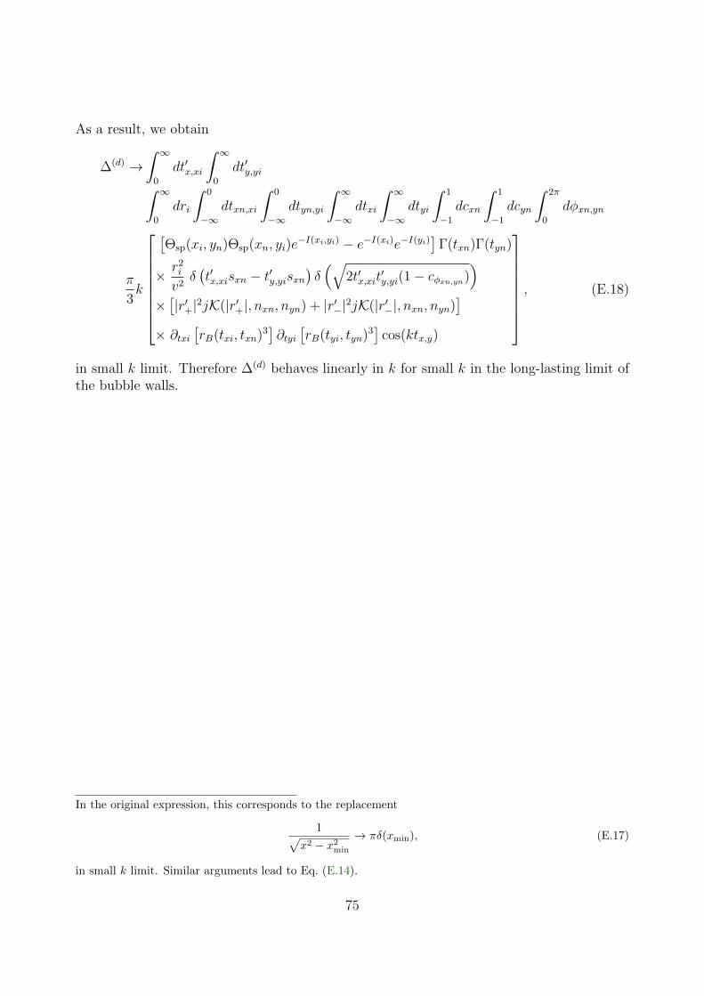
As a result, we obtain

∆(d) →∫ ∞

0

dt′x,xi

∫ ∞0

dt′y,yi∫ ∞0

dri

∫ 0

−∞dtxn,xi

∫ 0

−∞dtyn,yi

∫ ∞−∞

dtxi

∫ ∞−∞

dtyi

∫ 1

−1

dcxn

∫ 1

−1

dcyn

∫ 2π

0

dφxn,yn

π

3k

[Θsp(xi, yn)Θsp(xn, yi)e

−I(xi,yi) − e−I(xi)e−I(yi)]

Γ(txn)Γ(tyn)

× r2i

v2δ(t′x,xisxn − t′y,yisxn

)δ(√

2t′x,xit′y,yi(1− cφxn,yn)

)×[|r′+|2jK(|r′+|, nxn, nyn) + |r′−|2jK(|r′−|, nxn, nyn)

]× ∂txi

[rB(txi, txn)3

]∂tyi

[rB(tyi, tyn)3

]cos(ktx,y)

, (E.18)

in small k limit. Therefore ∆(d) behaves linearly in k for small k in the long-lasting limit ofthe bubble walls.

In the original expression, this corresponds to the replacement

1√x2 − x2min

→ πδ(xmin), (E.17)

in small k limit. Similar arguments lead to Eq. (E.14).

75

F Useful equations

In this appendix we summarize useful formulas. In performing the angular part of the Fouriertransformation with respect to ~r, the following formula holds for arbitrary unit vectors nxand ny, which are defined through their angles measured from ~r (see Fig. 14):♦47

∫dΩr

∫ 2π

0

dφ〈x,y〉 Kijkl(k)ei~k·~rNijkl

= 4π2

[j0(kr)K0(nx, ny) +

j1(kr)

krK1(nx, ny) +

j2(kr)

(kr)2K2(nx, ny)

]. (F.2)

Here φ〈x,y〉 ≡ (φx + φy)/2, and Kn are

K0(nx, ny) = s2xs

2y cos(2(φx − φy)), (F.3)

K1(nx, ny) = 8sxcxsycy cos(φx − φy)− 2s2xs

2y cos(2(φx − φy)), (F.4)

K2(nx, ny) = 2(3c2x − 1)(3c2

y − 1)− 16sxcxsycy cos(φx − φy) + s2xs

2y cos(2(φx − φy)), (F.5)

with cx and sx (cy and sy) denoting cos θx and sin θx (cos θy and sin θy), Also, jn are thespherical Bessel functions

j0(x) =sinx

x, j1(x) =

sinx− x cosx

x2, j2(x) =

(3− x2) sinx− 3x cosx

x3. (F.6)

Note that the vectors nx and ny change their directions as ~r changes its direction becausethey are defined through their angles measured from ~r. The arguments θx, θy, φx and φy inEqs. (F.3)–(F.5) denote such angles.

G Other numerical results

In this appendix we show the results presented in Sec. 4 in terms of single- and double-bubblecontributions.

First, Figs. 27, 28 and 31 are the behavior of the single-bubble spectrum for v = 1.Fig. 27 shows the single-bubble spectrum as a function of the duration time τ for variouswavenumbers from k = 0.001 to 1. The blue, red, yellow and green lines denote k =(1, 0.6, 0.4, 0.2)×10−n (n ∈ Z), respectively. Fig. 28 is essentially the same as Fig. 27, exceptthat the horizontal axis is the wavenumber k. Different markers correspond to different τ ,and the black line is the single-bubble spectrum with the envelope approximation in Ref. [36].Fig. 31 shows the spectrum at fixed τ . The colored lines correspond to τ = 1, 3, 10, 30, 100from bottom to top, while the black-dashed line corresponds to τ = 10× (1/k). In making

♦47 The formula (F.2) can easily be derived by noting that∫dΩr

∫ 2π

0

dφ〈x,y〉 Kijkl(k)ei~k·~rNijkl =

∫dΩk

∫ 2π

0

dφ〈x,y〉 Kijkl(k)ei~k·~rNijkl. (F.1)

76

this figure we have interpolated the data points shown in Figs. 27 and 28 to make constant-τslices. Also, for large wavenumbers k > 0.1, we have extrapolated the value at τ = 10×(1/k)to larger τ by assuming that the spectrum is constant after this time.

Next, Figs. 29, 30 and 32 are the same as Figs. 27, 28 and 31, respectively, except thatthey show the double-bubble spectrum. It is seen that the single-bubble dominates thedouble-bubble for the wavenumbers shown in the plot.

Finally, Figs. 33, 34 and 37 are the behavior of the single-bubble spectrum for v = cs,which correspond to Figs. 27, 28 and 31, respectively. The basic features are the same asv = 1 case. Also, Figs. 35, 36 and 38 show the double-bubble spectrum for v = cs.

H Comment on “spherical symmetry”

In this appendix we explain why the single-bubble contribution arises in spite of the factthat spherically symmetric objects do not radiate GWs.

Let us take the single-bubble contribution in the envelope case as an example. See Fig. 39.In this figure we take the evaluation times to satisfy tx = ty for an illustrative purpose. Thepoint is that, in the formalism illustrated in Sec. 3 and used in Appendix A–C, we do notscan the spacetime points x and y over the surface of a single bubble but rather first fix themand then sum up all the bubble configurations which gives nonzero T (x)T (y). One sees thatthe spherical symmetry of a single bubble is in fact broken by the process of fixing x and y:the bubble wall fragments propagating towards ~x and ~y cannot collide with other walls untilthe evaluation time (note that walls instantly disappear when they collide with each otherwithin the envelope approximation), while other parts of the wall can collide before thattime, as shown in Fig. 39. Therefore, our formalism automatically takes into account thebreaking of the spherical symmetry of each bubble caused by collisions with other bubbles.

77

10-2

100

102

104

10-8

10-6

10-4

10-2

1

(s)

100

10-1

10-2

10-3

Figure 27: The single-bubble spectrum ∆(s) as a function of the duration time τ for v = 1. Theblue, red, yellow and green lines correspond to k = (1, 0.6, 0.4, 0.2)× 10−n (n ∈ Z), respectively.

10-3

10-2

10-1

100

k/

10-8

10-6

10-4

10-2

1

(s)

=0.01×(k/)-1 =0.03×(k/)-1 =0.1×(k/)-1 =0.3×(k/)-1

=1×(k/)-1 =3×(k/)-1 =10×(k/)-1

Figure 28: The single-bubble spectrum ∆(s) as a function of wavenumber k for v = 1. Eachdata point corresponds to τ = (0.01, 0.03, 0.1, 0.3, 1, 3, 10) × (1/k), while the black line shows thesingle-bubble spectrum with the envelope approximation in Ref. [36].

78

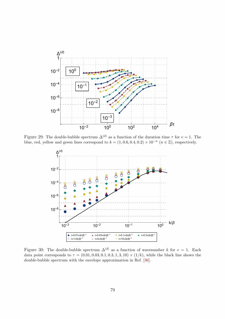
10-2

100

102

104

10-8

10-6

10-4

10-2

1

(d)

100

10-1

10-2

10-3

Figure 29: The double-bubble spectrum ∆(d) as a function of the duration time τ for v = 1. Theblue, red, yellow and green lines correspond to k = (1, 0.6, 0.4, 0.2)× 10−n (n ∈ Z), respectively.

10-3

10-2

10-1

100

k/

10-8

10-6

10-4

10-2

1

(d)

=0.01×(k/)-1 =0.03×(k/)-1 =0.1×(k/)-1 =0.3×(k/)-1

=1×(k/)-1 =3×(k/)-1 =10×(k/)-1

Figure 30: The double-bubble spectrum ∆(d) as a function of wavenumber k for v = 1. Eachdata point corresponds to τ = (0.01, 0.03, 0.1, 0.3, 1, 3, 10) × (1/k), while the black line shows thedouble-bubble spectrum with the envelope approximation in Ref. [36].

79

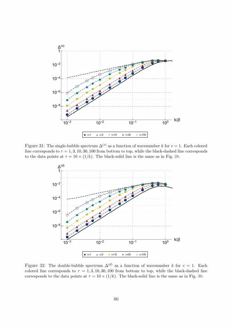
10-3

10-2

10-1

100

k/

10-8

10-6

10-4

10-2

1

(s)

=1 =3 =10 =30 =100

Figure 31: The single-bubble spectrum ∆(s) as a function of wavenumber k for v = 1. Each coloredline corresponds to τ = 1, 3, 10, 30, 100 from bottom to top, while the black-dashed line correspondsto the data points at τ = 10× (1/k). The black-solid line is the same as in Fig. 28.

10-3

10-2

10-1

100

k/

10-8

10-6

10-4

10-2

1

(d)

=1 =3 =10 =30 =100

Figure 32: The double-bubble spectrum ∆(d) as a function of wavenumber k for v = 1. Eachcolored line corresponds to τ = 1, 3, 10, 30, 100 from bottom to top, while the black-dashed linecorresponds to the data points at τ = 10× (1/k). The black-solid line is the same as in Fig. 30.

80

10-2

100

102

104

10-8

10-6

10-4

10-2

1

(s)

100

10-1

10-2

10-3

Figure 33: Same as Fig. 27 except that v = cs.

10-3

10-2

10-1

100

k/

10-8

10-6

10-4

10-2

1

(s)

=0.01×(k/)-1 =0.03×(k/)-1 =0.1×(k/)-1 =0.3×(k/)-1

=1×(k/)-1 =3×(k/)-1 =10×(k/)-1

Figure 34: Same as Fig. 28 except that v = cs.

81

10-2

100

102

104

10-8

10-6

10-4

10-2

1

(d)

100

10-1

10-2

10-3

Figure 35: Same as Fig. 29 except that v = cs.

10-3

10-2

10-1

100

k/

10-8

10-6

10-4

10-2

1

(d)

=0.01×(k/)-1 =0.03×(k/)-1 =0.1×(k/)-1 =0.3×(k/)-1

=1×(k/)-1 =3×(k/)-1 =10×(k/)-1

Figure 36: Same as Fig. 30 except that v = cs.

82

10-3

10-2

10-1

100

k/

10-8

10-6

10-4

10-2

1

(s)

=1 =3 =10 =30 =100

Figure 37: Same as Fig. 31 except that v = cs.

10-3

10-2

10-1

100

k/

10-8

10-6

10-4

10-2

1

(d)

=1 =3 =10 =30 =100

Figure 38: Same as Fig. 32 except that v = cs.

83

Figure 39: Illustration for why the single-bubble contribution arises in spite of the sphericalsymmetry of a single bubble. In this figure we show the envelope case and set tx = ty. Same figureas in Ref. [36].

84

References

[1] A. A. Starobinsky, “Spectrum of relict gravitational radiation and the early state of theuniverse,” JETP Lett. 30 (1979) 682–685. [Pisma Zh. Eksp. Teor. Fiz.30,719(1979)].

[2] S. Y. Khlebnikov and I. I. Tkachev, “Relic gravitational waves produced after preheating,”Phys. Rev. D56 (1997) 653–660, arXiv:hep-ph/9701423 [hep-ph].

[3] A. Vilenkin and E. P. S. Shellard, Cosmic Strings and Other Topological Defects. CambridgeUniversity Press, 2000. http://www.cambridge.org/mw/academic/subjects/physics/theoretical-physics-and-mathematical-physics/

cosmic-strings-and-other-topological-defects?format=PB.

[4] E. Witten, “Cosmic Separation of Phases,” Phys. Rev. D30 (1984) 272–285.

[5] C. J. Hogan, “Gravitational radiation from cosmological phase transitions,” Mon. Not. Roy.Astron. Soc. 218 (1986) 629–636.

[6] Virgo, LIGO Scientific Collaboration, B. P. Abbott et al., “Observation of GravitationalWaves from a Binary Black Hole Merger,” Phys. Rev. Lett. 116 no. 6, (2016) 061102,arXiv:1602.03837 [gr-qc].

[7] Virgo, LIGO Scientific Collaboration, B. P. Abbott et al., “GW151226: Observation ofGravitational Waves from a 22-Solar-Mass Binary Black Hole Coalescence,” Phys. Rev. Lett.116 no. 24, (2016) 241103, arXiv:1606.04855 [gr-qc].

[8] VIRGO, LIGO Scientific Collaboration, B. P. Abbott et al., “GW170104: Observation ofa 50-Solar-Mass Binary Black Hole Coalescence at Redshift 0.2,” Phys. Rev. Lett. 118no. 22, (2017) 221101, arXiv:1706.01812 [gr-qc].

[9] eLISA Collaboration, P. A. Seoane et al., “The Gravitational Universe,” arXiv:1305.5720

[astro-ph.CO].

[10] G. M. Harry, P. Fritschel, D. A. Shaddock, W. Folkner, and E. S. Phinney, “Laserinterferometry for the big bang observer,” Class. Quant. Grav. 23 (2006) 4887–4894.[Erratum: Class. Quant. Grav.23,7361(2006)].

[11] N. Seto, S. Kawamura, and T. Nakamura, “Possibility of direct measurement of theacceleration of the universe using 0.1-Hz band laser interferometer gravitational wave antennain space,” Phys. Rev. Lett. 87 (2001) 221103, arXiv:astro-ph/0108011 [astro-ph].

[12] K. Kajantie, M. Laine, K. Rummukainen, and M. E. Shaposhnikov, “Is there a hotelectroweak phase transition at m(H) larger or equal to m(W)?,” Phys. Rev. Lett. 77 (1996)2887–2890, arXiv:hep-ph/9605288 [hep-ph].

[13] M. Gurtler, E.-M. Ilgenfritz, and A. Schiller, “Where the electroweak phase transition ends,”Phys. Rev. D56 (1997) 3888–3895, arXiv:hep-lat/9704013 [hep-lat].

[14] F. Csikor, Z. Fodor, and J. Heitger, “Endpoint of the hot electroweak phase transition,”Phys. Rev. Lett. 82 (1999) 21–24, arXiv:hep-ph/9809291 [hep-ph].

85

[15] C. Caprini et al., “Science with the space-based interferometer eLISA. II: Gravitationalwaves from cosmological phase transitions,” JCAP 1604 no. 04, (2016) 001,arXiv:1512.06239 [astro-ph.CO].

[16] R.-G. Cai, Z. Cao, Z.-K. Guo, S.-J. Wang, and T. Yang, “The Gravitational-Wave Physics,”arXiv:1703.00187 [gr-qc].

[17] A. Kosowsky, M. S. Turner, and R. Watkins, “Gravitational radiation from colliding vacuumbubbles,” Phys. Rev. D45 (1992) 4514–4535.

[18] A. Kosowsky, M. S. Turner, and R. Watkins, “Gravitational waves from first ordercosmological phase transitions,” Phys. Rev. Lett. 69 (1992) 2026–2029.

[19] A. Kosowsky and M. S. Turner, “Gravitational radiation from colliding vacuum bubbles:envelope approximation to many bubble collisions,” Phys. Rev. D47 (1993) 4372–4391,arXiv:astro-ph/9211004 [astro-ph].

[20] M. Kamionkowski, A. Kosowsky, and M. S. Turner, “Gravitational radiation from first orderphase transitions,” Phys. Rev. D49 (1994) 2837–2851, arXiv:astro-ph/9310044[astro-ph].

[21] S. J. Huber and T. Konstandin, “Gravitational Wave Production by Collisions: MoreBubbles,” JCAP 0809 (2008) 022, arXiv:0806.1828 [hep-ph].

[22] M. Hindmarsh, S. J. Huber, K. Rummukainen, and D. J. Weir, “Gravitational waves fromthe sound of a first order phase transition,” Phys. Rev. Lett. 112 (2014) 041301,arXiv:1304.2433 [hep-ph].

[23] M. Hindmarsh, S. J. Huber, K. Rummukainen, and D. J. Weir, “Numerical simulations ofacoustically generated gravitational waves at a first order phase transition,” Phys. Rev. D92no. 12, (2015) 123009, arXiv:1504.03291 [astro-ph.CO].

[24] M. Hindmarsh, S. J. Huber, K. Rummukainen, and D. J. Weir, “Shape of the acousticgravitational wave power spectrum from a first order phase transition,” arXiv:1704.05871

[astro-ph.CO].

[25] H. L. Child and J. T. Giblin, Jr., “Gravitational Radiation from First-Order PhaseTransitions,” JCAP 1210 (2012) 001, arXiv:1207.6408 [astro-ph.CO].

[26] J. T. Giblin, Jr. and J. B. Mertens, “Vacuum Bubbles in the Presence of a RelativisticFluid,” JHEP 12 (2013) 042, arXiv:1310.2948 [hep-th].

[27] J. T. Giblin and J. B. Mertens, “Gravitional radiation from first-order phase transitions inthe presence of a fluid,” Phys. Rev. D90 no. 2, (2014) 023532, arXiv:1405.4005[astro-ph.CO].

[28] A. Kosowsky, A. Mack, and T. Kahniashvili, “Gravitational radiation from cosmologicalturbulence,” Phys. Rev. D66 (2002) 024030, arXiv:astro-ph/0111483 [astro-ph].

[29] A. Nicolis, “Relic gravitational waves from colliding bubbles and cosmic turbulence,” Class.Quant. Grav. 21 (2004) L27, arXiv:gr-qc/0303084 [gr-qc].

86

[30] C. Caprini and R. Durrer, “Gravitational waves from stochastic relativistic sources:Primordial turbulence and magnetic fields,” Phys. Rev. D74 (2006) 063521,arXiv:astro-ph/0603476 [astro-ph].

[31] C. Caprini, R. Durrer, and G. Servant, “The stochastic gravitational wave background fromturbulence and magnetic fields generated by a first-order phase transition,” JCAP 0912(2009) 024, arXiv:0909.0622 [astro-ph.CO].

[32] T. Kahniashvili, L. Kisslinger, and T. Stevens, “Gravitational Radiation Generated byMagnetic Fields in Cosmological Phase Transitions,” Phys. Rev. D81 (2010) 023004,arXiv:0905.0643 [astro-ph.CO].

[33] D. J. Weir, “Revisiting the envelope approximation: gravitational waves from bubblecollisions,” Phys. Rev. D93 no. 12, (2016) 124037, arXiv:1604.08429 [astro-ph.CO].

[34] M. Hindmarsh, “Sound shell model for acoustic gravitational wave production at a first-orderphase transition in the early Universe,” arXiv:1608.04735 [astro-ph.CO].

[35] C. Caprini, R. Durrer, and G. Servant, “Gravitational wave generation from bubble collisionsin first-order phase transitions: An analytic approach,” Phys. Rev. D77 (2008) 124015,arXiv:0711.2593 [astro-ph].

[36] R. Jinno and M. Takimoto, “Gravitational waves from bubble collisions: analyticderivation,” Phys. Rev. D95 no. 2, (2017) 024009, arXiv:1605.01403 [astro-ph.CO].

[37] R. Jinno, S. Lee, H. Seong, and M. Takimoto, work in progress.

[38] J. R. Espinosa, T. Konstandin, J. M. No, and G. Servant, “Energy Budget of CosmologicalFirst-order Phase Transitions,” JCAP 1006 (2010) 028, arXiv:1004.4187 [hep-ph].

[39] L. Leitao and A. Megevand, “Hydrodynamics of ultra-relativistic bubble walls,” Nucl. Phys.B905 (2016) 45–72, arXiv:1510.07747 [astro-ph.CO].

[40] D. Bodeker and G. D. Moore, “Can electroweak bubble walls run away?,” JCAP 0905(2009) 009, arXiv:0903.4099 [hep-ph].

[41] D. Bodeker and G. D. Moore, “Electroweak Bubble Wall Speed Limit,” JCAP 1705 no. 05,(2017) 025, arXiv:1703.08215 [hep-ph].

[42] A. Megevand and S. Ramirez, “Bubble nucleation and growth in very strong cosmologicalphase transitions,” Nucl. Phys. B919 (2017) 74–109, arXiv:1611.05853 [astro-ph.CO].

[43] A. D. Linde, “On the Vacuum Instability and the Higgs Meson Mass,” Phys. Lett. B70(1977) 306–308.

[44] A. D. Linde, “Decay of the False Vacuum at Finite Temperature,” Nucl. Phys. B216 (1983)421. [Erratum: Nucl. Phys.B223,544(1983)].

[45] T. Hahn, “CUBA: A Library for multidimensional numerical integration,” Comput. Phys.Commun. 168 (2005) 78–95, arXiv:hep-ph/0404043 [hep-ph].

[46] M. S. Turner, E. J. Weinberg, and L. M. Widrow, “Bubble nucleation in first order inflationand other cosmological phase transitions,” Phys. Rev. D46 (1992) 2384–2403.

87