
Gravitational softening as a smoothing operationbarnes/research/smoothing/soft_ds.pdfMon. Not. R....
29
Mon. Not. R. Astron. Soc. 000, 000–000 (0000) Printed 24 August 2012 (MN L A T E X style file v2.2) Gravitational softening as a smoothing operation Joshua E. Barnes Institute of Astronomy, University of Hawaii, 2680 Woodlawn Drive, Honolulu, HI 96822, USA 24 August 2012 ABSTRACT In self-consistent N -body simulations of collisionless systems, gravitational interactions are modified on small scales to remove singularities and simplify the task of numerically integrating the equations of motion. This ‘gravitational softening’ is sometimes presented as an ad-hoc departure from Newtonian gravity. However, softening can also be described as a smoothing operation applied to the mass distribution; the gravitational potential and the smoothed density obey Poisson’s equation precisely. While ‘softening’ and ‘smoothing’ are mathematically equivalent descriptions, the latter has some advantages. For example, the smoothing description suggests a way to set up N -body initial conditions in almost perfect dynamical equilibrium. Key words: methods: numerical – galaxies: kinematics & dynamics 1 INTRODUCTION The evolution of a collisionless self-gravitating system is described by two coupled equations: the Vlasov equation, ∂f ∂t + v · ∂f ∂ r -∇Φ · ∂f ∂ v =0 , (1) where f = f (r, v,t) is the one-particle distribution function and Φ(r,t) is the gravitational potential, and Poisson’s equation, ∇ 2 Φ=4πGρ =4πG dv f. (2) N -body simulations use a Monte-Carlo method to solve these equations. The distribution function is represented by a collection of N particles (Klimontovich 1967): f (r, v,t)= N i=1 m i δ 3 (r - r i (t)) δ 3 (v - v i (t)) , (3) c 0000 RAS
Transcript of Gravitational softening as a smoothing operationbarnes/research/smoothing/soft_ds.pdfMon. Not. R....

Mon. Not. R. Astron. Soc. 000, 000–000 (0000) Printed 24 August 2012 (MN LATEX style file v2.2)
Gravitational softening as a smoothing operation
Joshua E. BarnesInstitute of Astronomy, University of Hawaii, 2680 Woodlawn Drive, Honolulu, HI 96822, USA
24 August 2012
ABSTRACT
In self-consistent N -body simulations of collisionless systems, gravitational
interactions are modified on small scales to remove singularities and simplify
the task of numerically integrating the equations of motion. This ‘gravitational
softening’ is sometimes presented as an ad-hoc departure from Newtonian
gravity. However, softening can also be described as a smoothing operation
applied to the mass distribution; the gravitational potential and the smoothed
density obey Poisson’s equation precisely. While ‘softening’ and ‘smoothing’
are mathematically equivalent descriptions, the latter has some advantages.
For example, the smoothing description suggests a way to set up N -body
initial conditions in almost perfect dynamical equilibrium.
Key words: methods: numerical – galaxies: kinematics & dynamics
1 INTRODUCTION
The evolution of a collisionless self-gravitating system is described by two coupled equations:
the Vlasov equation,
!f
!t+ v · !f
!r!"! · !f
!v= 0 , (1)
where f = f(r,v, t) is the one-particle distribution function and !(r, t) is the gravitational
potential, and Poisson’s equation,
"2! = 4"G# = 4"G!
dv f . (2)
N -body simulations use a Monte-Carlo method to solve these equations. The distribution
function is represented by a collection of N particles (Klimontovich 1967):
f(r,v, t) =N"
i=1
mi $3(r ! ri(t)) $
3(v ! vi(t)) , (3)
c! 0000 RAS
2 J. E. Barnes
where mi, ri, and vi are the mass, position, and velocity of particle i. Over time, particles
move along characteristics of (1); at each instant, their positions provide the density needed
for (2).
In many collisionless N -body simulations, the equations of motion actually integrated
are
dri
dt= vi ,
dvi
dt=
N"
j "=i
Gmjrj ! ri
(|rj ! ri|2 + %2)3/2, (4)
where % is the softening length. These equations reduce to the standard Newtonian equations
of motion if % = 0. The main reason for setting % #= 0 is to suppress the 1/r singularity in
the Newtonian potential; this greatly simplifies the task of numerically integrating these
equations (e.g., Dehnen 2001). By limiting the spatial resolution of the gravitational force,
softening also helps control fluctuations caused by sampling the distribution function with
finite N ; however, this comes at a price, since the gravitational field is systematically biased
for % #= 0 (Merritt 1996; Athanassoula et al. 1998, 2000).
Softening is often described as a modification of Newtonian gravity, with the 1/r potential
replaced by 1/$
r2 + %2. The latter is proportional to the potential of a Plummer (1911)
sphere with scale radius %. This does not imply that particles interact like Plummer spheres
(Dyer & Ip 1993); the acceleration of particle i is computed from the field at the point
ri only. But it does imply that softening can also be described as a smoothing operation
(e.g., Hernquist & Barnes 1990), in which the pointillistic Monte-Carlo representation of the
density field is convolved with the kernel
S(r; %) =3
4"
%2
(r2 + %2)5/2. (5)
In e"ect, the source term for Poisson’s equation (2) is replaced with the smoothed density
#(r; %) %!
dr# #(r#)S(|r! r#|; %) =!
dr# #(r ! r#)S(|r#|; %) . (6)
Formally, (4) provides a Monte-Carlo solution to the Vlasov equation (1) coupled with
"2! = 4"G#(r; %) = 4"G!
dr#!
dv f(r#,v, t)S(|r! r#|; %) . (7)
Thus one may argue that a softened N -body simulation actually uses standard Newtonian
gravity, as long as it is clear that the mass distribution generating the gravitational field is
derived from the particles via a smoothing process.
Although Plummer softening is widely used in N -body simulations, its e"ects are incom-
pletely understood. If the underlying density field is featureless on scales of order %, softening
c! 0000 RAS, MNRAS 000, 000–000
Softening as Smoothing 3
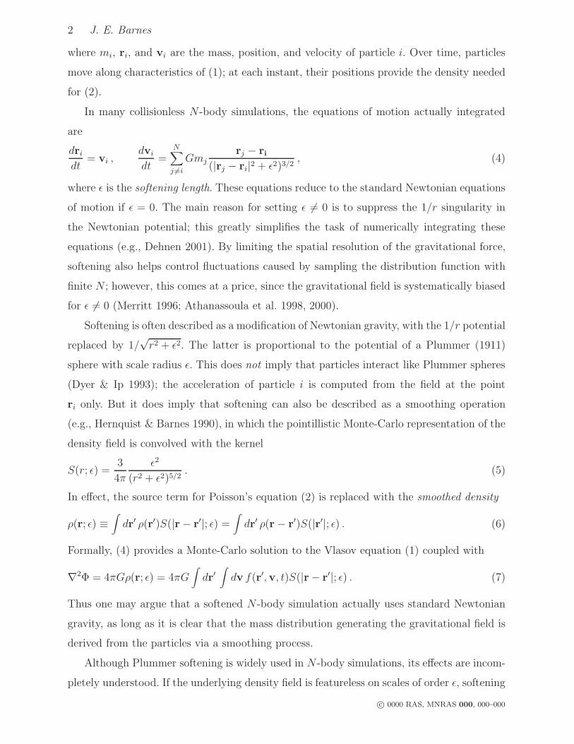
Figure 1. E!ect of Plummer smoothing on a ! $ r!1
profile. Dashed line is the underlying density profile; solidcurve is the result of smoothing with " = 1. The smoothedprofile is always less than the underlying power-law.
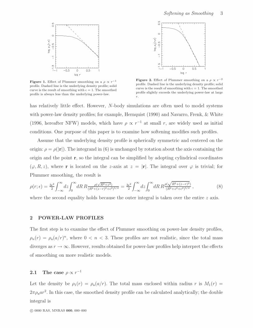
Figure 2. E!ect of Plummer smoothing on a ! $ r!2
profile. Dashed line is the underlying density profile; solidcurve is the result of smoothing with " = 1. The smoothedprofile slightly exceeds the underlying power-law at larger.
has relatively little e"ect. However, N -body simulations are often used to model systems
with power-law density profiles; for example, Hernquist (1990) and Navarro, Frenk, & White
(1996, hereafter NFW) models, which have # & r%1 at small r, are widely used as initial
conditions. One purpose of this paper is to examine how softening modifies such profiles.
Assume that the underlying density profile is spherically symmetric and centered on the
origin: # = #(|r|). The integrand in (6) is unchanged by rotation about the axis containing the
origin and the point r, so the integral can be simplified by adopting cylindrical coordinates
(&, R, z), where r is located on the z-axis at z = |r|. The integral over & is trivial; for
Plummer smoothing, the result is
#(r; %) = 3"2
2
! &
%&dz
! &
0dR R !(
'R2+z2)
(R2+(z%r)2+"2)5/2 = 3"2
2
! &
%&dz
! &
0dR R
!($
R2+(z%r)2)
(R2+z2+"2)5/2 , (8)
where the second equality holds because the outer integral is taken over the entire z axis.
2 POWER-LAW PROFILES
The first step is to examine the e"ect of Plummer smoothing on power-law density profiles,
#n(r) = #a(a/r)n, where 0 < n < 3. These profiles are not realistic, since the total mass
diverges as r ' (. However, results obtained for power-law profiles help interpret the e"ects
of smoothing on more realistic models.
2.1 The case # & r%1
Let the density be #1(r) = #a(a/r). The total mass enclosed within radius r is M1(r) =
2"#aar2. In this case, the smoothed density profile can be calculated analytically; the double
integral is
c! 0000 RAS, MNRAS 000, 000–000
4 J. E. Barnes
! &
%&dz
! &
0dR R
(R2 + (z ! r)2)%1/2
(R2 + z2 + %2)5/2=
2
3%2$%2 + r2
. (9)
This yields a remarkably simple result for the smoothed density, plotted in Fig. 1,
#1(r; %) = #aa$
%2 + r2= #1(
$%2 + r2) = #1(r") , (10)
where r" %$%2 + r2. The smoothed mass within radius r, hereafter called the smoothed
mass profile1, is
M1(r; %) =! r
0dx 4"x2 #1(x; %) = 2"#aa
#rr" ! %2 sinh%1(r/%)
$. (11)
2.2 The case # & r%2
Let the density be #2(r) = #a(a/r)2. The total mass enclosed within radius r is M2(r) =
4"#aa2r. The integral over R can be evaluated, but the result is not particularly informa-
tive and the remaining integral must be done numerically. Fig. 2 presents the results. For
log(r) >) 0.2, the smoothed density exceeds the underlying power-law profile. This occurs be-
cause smoothing, in e"ect, spreads mass from r <) % to larger radii, and with the underlying
profile dropping away so steeply this redistributed mass makes a relatively large contribution
to #2(r; %). Note that as r ' 0, the smoothed density #2(r; %) ' 2#2(%).
2.3 Central density
It appears impossible to calculate the smoothed density profile for arbitrary n without
resorting to numerical methods, but the central density is another matter. Setting r = 0,
the smoothed density is
#n(0; %) = 3%2! &
0dx
x2#n(x)
(x2 + %2)5/2=
n$"#(3
2 !n2 )#(n
2 )#n(%) . (12)
The central density ratio D0(n) = #n(0; %)/#n(%) is plotted as a function of n in Fig. 3. For
n = 1 and 2, the ratio D0 = 1 and 2, respectively, in accord with the results above, while as
n ' 3 the central density diverges.
The smoothed central density for an arbitrary power-law is useful in devising an approx-
imate expression for the smoothed density profile (Appendix A.1). In addition, the central
density is related to the shortest dynamical time-scale present in an N -body simulation,
which may in turn be used to estimate a maximum permissible value for the time-step
(§ 4.3.1).
1 This profile can’t be obtained by applying kernel smoothing directly to M(r); only density profiles can be smoothed.
c! 0000 RAS, MNRAS 000, 000–000

Softening as Smoothing 5
Figure 3. Density ratio D0 = !n(0; ")/!n(") plotted as a function of n. Limiting values are D0 = 1 as n ( 0 and D0 = & asn ( 3.
3 ASTROPHYSICAL MODELS
3.1 Hernquist and NFW models
As noted above, both of these profiles have # & r%1 as r ' 0. For this reason, they are
treated in parallel. The Hernquist (1990) model has density and mass profiles
#H(r) =aM
2"r(a + r)3, MH(r) =
Mr2
(r + a)2, (13)
where a is the scale radius and M is the total mass. The Navarro, Frenk, & White (1996)
model has density and mass profiles
#NFW(r) =a3#0
r(a + r)2, MNFW(r) = 4"#0a
3%log
%a + r
a
&! r
a + r
&, (14)
where a is again the scale radius and #0 is a characteristic density. The double integrals
required to evaluate the smoothed versions of these profiles appear intractable analytically2
but can readily be calculated numerically. Figs. 4 and 5 present results for a range of % values
between a and a/256. For comparison, both models are scaled to have the same underlying
density profile at r * a.
The smoothed profiles shown in Figs. 4 and 5 are, for the most part, easily understood in
terms of the results obtained for power-laws. For radii r < %, smoothing transforms central
cusps into constant-density cores, just as in Fig. 1. If the softening length % is much less than
the scale length a, the smoothed density #(r; %) within r * a is almost independent of the
underlying profile at radii r > a. Consequently, the smoothed central density #(0; %) + #(%),
echoing the result obtained for the power-law n = 1. In addition, the actual curves in
Figs. 4 and 5 are shifted versions of the curves in Fig. 1; this observation motivates simple
approximations to #H(r; %) and #NFW(r; %) described in Appendix A.2.
2 Smoothed central densities for these and other profiles can be expressed in terms of special functions.
c! 0000 RAS, MNRAS 000, 000–000

6 J. E. Barnes
Figure 4. E!ect of Plummer smoothing on Hernquistprofile. Top curve shows the density profile of a Hernquistmodel with scale radius a = 1 and mass M = 1. Lowercurves show profiles smoothed with " = 1/256, 1/128, . . . ,1 (from top to bottom); heavy curve is " = 1/64, dashedcurve is " = 1. Inset shows ratio !H(r; ")/!H(r).
Figure 5. E!ect of Plummer smoothing on NFW profile.Top curve shows the density profile of a NFW model withscale radius a = 1 and density !0 = 1/(2#). Lower curvesshow profiles smoothed with " = 1/256, 1/128, . . . , 1(from top to bottom); heavy curve is " = 1/64, dashedcurve is " = 1. Inset shows ratio !NFW(r; ")/!NFW(r).
On the other hand, if % is comparable to a, the quantitative agreement between these
profiles and the smoothed n = 1 profile breaks down; the smoothed density at small r has
a non-negligible contribution from the underlying profile beyond the scale radius a. As an
example, for % = 1 the central density of the smoothed NFW profile is higher than the central
density of the smoothed Hernquist profile, because the former receives a larger contribution
from mass beyond the scale radius.
A somewhat more subtle result, shown in the insets, is that heavily smoothed profiles
exceed the underlying profiles at radii r >) a. This is basically the same e"ect found with the
n = 2 power-law profile (§ 2.2); with the underlying density dropping rapidly as a function
of r, the mass spread outward from smaller radii more than makes up for the mass spread
to still larger radii. This e"ect is more evident for the Hernquist profile than for the NFW
profile because the former falls o" more steeply for r >) a.
3.2 Ja!e model
The Ja"e (1983) model has density and mass profiles
#J(r) =aM
4"r2(a + r)2, MJ(r) =
Mr
(r + a), (15)
c! 0000 RAS, MNRAS 000, 000–000
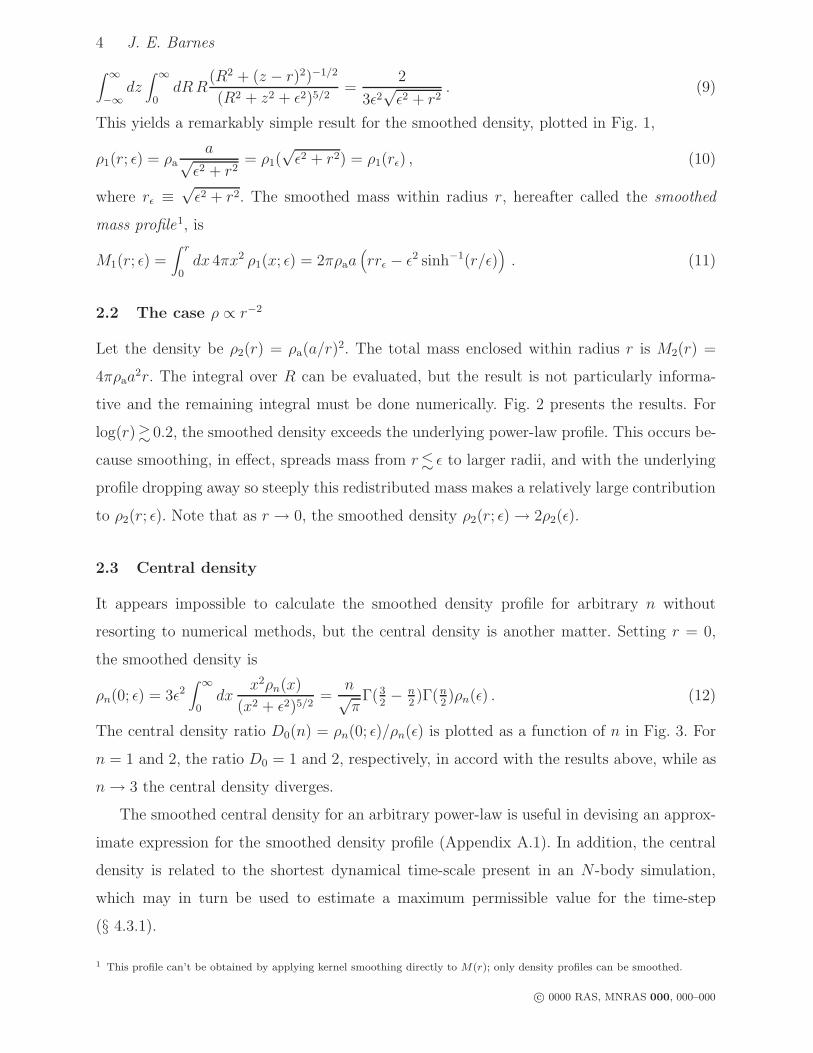
Softening as Smoothing 7
Figure 6. E!ect of Plummer smoothing on Ja!e profile.Top curve shows the density profile of a Ja!e model withscale radius a = 1 and mass M = 1. Lower curves showprofiles smoothed with " = 1/256, 1/128, . . . , 1 (fromtop to bottom); heavy curve is " = 1/64, dashed curve is" = 1. Inset shows ratio !J(r; ")/!J(r).
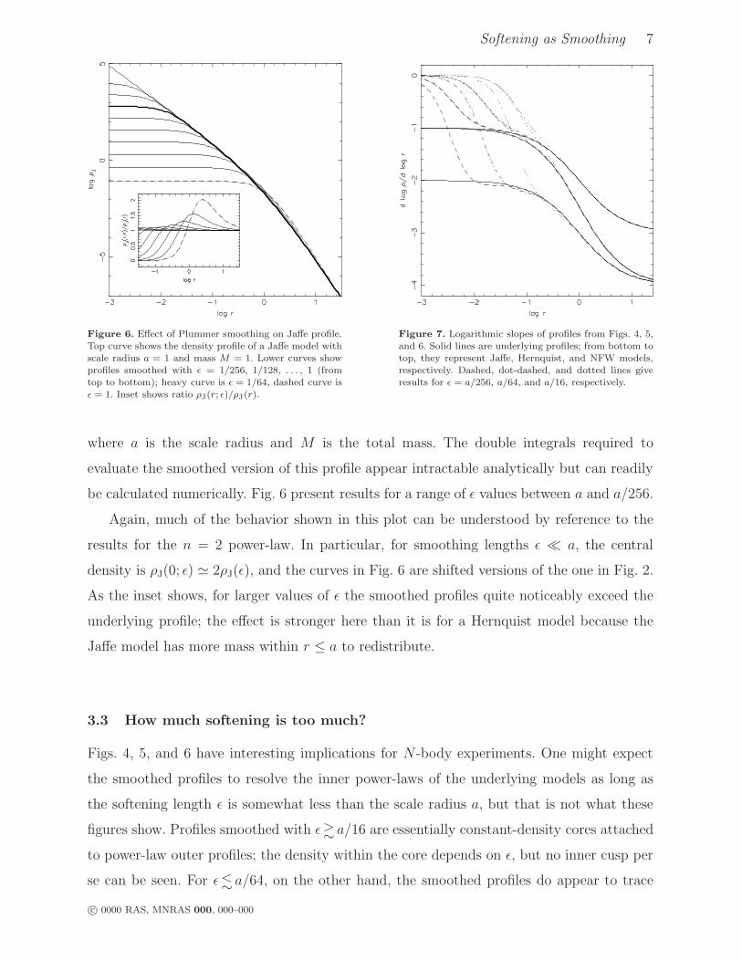
Figure 7. Logarithmic slopes of profiles from Figs. 4, 5,and 6. Solid lines are underlying profiles; from bottom totop, they represent Ja!e, Hernquist, and NFW models,respectively. Dashed, dot-dashed, and dotted lines giveresults for " = a/256, a/64, and a/16, respectively.
where a is the scale radius and M is the total mass. The double integrals required to
evaluate the smoothed version of this profile appear intractable analytically but can readily
be calculated numerically. Fig. 6 present results for a range of % values between a and a/256.
Again, much of the behavior shown in this plot can be understood by reference to the
results for the n = 2 power-law. In particular, for smoothing lengths % * a, the central
density is #J(0; %) + 2#J(%), and the curves in Fig. 6 are shifted versions of the one in Fig. 2.
As the inset shows, for larger values of % the smoothed profiles quite noticeably exceed the
underlying profile; the e"ect is stronger here than it is for a Hernquist model because the
Ja"e model has more mass within r , a to redistribute.
3.3 How much softening is too much?
Figs. 4, 5, and 6 have interesting implications for N -body experiments. One might expect
the smoothed profiles to resolve the inner power-laws of the underlying models as long as
the softening length % is somewhat less than the scale radius a, but that is not what these
figures show. Profiles smoothed with %>) a/16 are essentially constant-density cores attached
to power-law outer profiles; the density within the core depends on %, but no inner cusp per
se can be seen. For %<) a/64, on the other hand, the smoothed profiles do appear to trace
c! 0000 RAS, MNRAS 000, 000–000
8 J. E. Barnes
the inner power-laws over some finite range of radii, before flattening out at smaller r. Only
for %<) a/256 can the inner cusps be followed for at least a decade in radius.
Fig. 7 helps explain this result. The underlying Ja"e, Hernquist, and NFW profiles all
roll over gradually from their inner to outer power-law slopes between radii 0.1a <) r <) 10a.
Thus a resolution somewhat better than 0.1a is required to see the inner cusps of these
models. In practice, this implies the softening parameter % must be several times smaller
than 0.1a.
4 TESTS AND APPLICATIONS
Since the formalism developed above is exact, numerical tests of a relation like (8) for the
smoothed density #(r; %) may seem superfluous. In practice, such tests can be illuminating
– as benchmarks of N -body technique. In what follows, the smoothing formalism will be
applied to actual N -body calculations, to check N -body methodology and to demonstrate
that the formalism has real applications.
Putting this plan into operation requires some care. To begin with, an N -body realization
of a standard Hernquist or Ja"e profile spans a huge range of radii. Typically, the innermost
particle has radius rin ) aN%1/2 or aN%1 for a Hernquist or Ja"e profile, respectively,
while for either profile, the outermost particle has radius rout ) aN . A dynamic range of
rout/rin ) N3/2 or N2 can be awkward to handle numerically; even gridless tree codes may
not accommodate such enormous ranges gracefully. One simple option is to truncate the
particle distribution at some fairly large radius, but it’s preferable to smoothly taper the
density profile:
#(r) ' #t(r) =
'(()
((*
(1 + µ) #(r) , r , b
(1 + µ) #) (b/r)2 e%r/r" , r > b
(16)
where the taper radius b - a, the values of r) and #) are fixed by requiring that #t(r) and
its first derivative are continuous at r = b, and the value of µ * 1 is chosen to preserve the
total mass. Let
' =r
#
d#
dr
+++++r=b
(17)
be the logarithmic slope of the density profile at r = b, and M(r) be the underlying mass
profile; then
c! 0000 RAS, MNRAS 000, 000–000
Softening as Smoothing 9
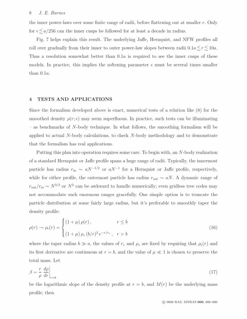
Figure 8. E!ect of Plummer smoothing on tapered Hernquist (left) and Ja!e (right) models, represented by the solid curves.Dashed, dot-dashed, and dotted curves show results for " = 1/256, 1/64, and 1/16, respectively.
r) =b
!(2 + '), #) = #(b)e%(2+$) , and µ =
M(()
M(b) + 4"b2r)#(b)! 1 . (18)
Fig. 8 shows how Plummer smoothing modifies tapered Hernquist and Ja"e profiles. Both
profiles have scale radius a = 1, taper radius b = 100, and mass M = 1; these parameters
will be used in all subsequent calculations. In each case, the underlying profile follows the
standard curve out to the taper radius b, and then rapidly falls away from the outer power
law. At radii r , b, the smoothed profiles match those shown in Figs. 4 and 6, apart from
the factor of (1 + µ) used to preserve total mass. At larger radii, the smoothed profiles
initially track the underlying tapered profiles, but then transition to asymptotic # & r%5
power law tails. This occurs because the Plummer smoothing kernel (5) falls o" as r%5 at
large r; in fact, these power laws match # = 3M%2/4"r5, which is the large-r approximation
for a point mass M smoothed with a Plummer kernel. The amount of mass in these r%5 tails
is negligible.
4.1 Gravitational potentials
In principle, it’s straightforward to verify that the smoothed profiles above generate poten-
tials matching those obtained from N -body calculations. For a given density profile #(r),
construct a realization with N particles at positions ri; a N -body force calculation with
softening % yields the gravitational potential !i for each particle. Conversely, given the
smoothed density profile #(r; %), compute the smoothed mass profile M(r; %), and use the
result to obtain the smoothed potential !(r; %):
c! 0000 RAS, MNRAS 000, 000–000

10 J. E. Barnes
d!
dr= G
M(r; %)
r2, (19)
with boundary condition !' 0 as r ' (. For each particle, the N -body potential !i may
be compared with the predicted value !(|ri|; %); apart from$
N fluctuations, the two should
agree.
A major complication is that$
N fluctuations in N -body realizations imprint spatially
coherent perturbations on the gravitational field; potentials measured at adjacent positions
are not statistically independent. For example, the softened potential at the origin of an
N -body system is
!0 ="
i
Gmi
(r2i + %2)1/2
. (20)
If the radii ri are independently chosen, this expression is a Monte Carlo integral, which will
deviate from !(0; %) by an amount of order O(N%1/2); moreover, everywhere within r <) %
the potential will deviate upward or downward by roughly as much as it does at r = 0.
One way around this is to average over many N -body realizations, but this is tedious and
expensive. An easier solution is to sample the radial distribution uniformly. Let M(r) be the
mass profile associated with the underlying density #(r). Assign all particles equal masses,
and determine the radius ri of particle i by solving M(ri) = (i ! 0.5)M(()/N for i = 1
to N . This eliminates radial fluctuations; the Monte-Carlo integral for !0 is replaced with
a panel integration uniformly spaced in M(r), and the central potential is obtained with
relatively high accuracy.
This trick does not suppress non-radial fluctuations, so the N -body potential evaluated
at any point r > 0 still di"ers from the true !(r; %). But a non-radial fluctuation which
creates an overdensity at some position rover must borrow mass from elsewhere on the sphere
r = |rover|; over-dense and under-dense regions compensate each other when averaged over
the entire surface of the sphere. The resulting potential fluctuations likewise average to zero
over the sphere, as one can show by using Gauss’s theorem to evaluate the average gradient
of the potential and integrating inward from r = (.
Finally, a subtle bias arises if the particles used to generate the potential are also used
to probe the potential, since local overdensities are sampled more heavily. To avoid this,
the potential can be measured at a set of points rk which are independent of the particle
positions ri. Then $!k % !k!!(rk; %) should display some scatter, but average to zero when
integrated over test points rk within a spherical shell.
c! 0000 RAS, MNRAS 000, 000–000
Softening as Smoothing 11
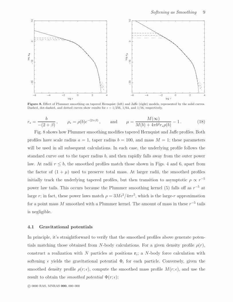
Figure 9. Di!erence %"k between N-body and smoothed potentials for tapered Hernquist (left) and Ja!e (right) models,normalized by central potential "(0; "). Vertical dashed lines show value of " = 1/64. Points are results for uniform realizations;jagged curves shows averages for groups of 32 points. Grey-scale images show typical results for random realizations. Centralpotentials are "H(0; ") = %0.9809 and "J(0; ") = %3.9009.
Fig. 9 shows results from direct-sum potential calculations for tapered Hernquist and
Ja"e models, using units with G = 1. In each case, the underlying density profile was rep-
resented with N = 220 = 1048576 equal-mass particles, and the potential was measured at
4096 points uniformly distributed in log(r) between 0.01% and 100%. The points show results
for uniform radial sampling. While non-radial fluctuations create scatter in !k, the distribu-
tion is fairly symmetric about the line $! = 0. The jagged curves are obtained by averaging
$!k over radial bins each containing 32 points. These averages fall near zero, demonstrating
very good agreement between the N -body results and the potentials calculated from the
smoothed density profiles.
For comparison, the grey-scale images in Fig. 9 display representative results for random
realizations of each density profile. In these realizations, the radius of particle i is computed
by solving M(ri) = XiM((), where Xi is a random number3 uniformly distributed between
0 and 1. To examine the range of outcomes, 1000 random realizations of each model were
generated and ranked by central potential !0; since particle radii are chosen independently,
the central limit theorem implies that !0 has a normal distribution. Shown here are the 25th
percentile and 75th percentile members of these ensembles; half of all random realizations lie
between the two examples presented in each figure. Note that these examples deviate from
3 A good random number generator is essential. The Unix generator, random(), appears to be slightly non-uniform; replacing
Xi with 1 % Xi yields systematically di!erent "0 values. The results shown here use the Tausworthe generator taus2 (Galassi
et al. 2009).
c! 0000 RAS, MNRAS 000, 000–000

12 J. E. Barnes
the true potential by fractional amounts of ) N%1/2. Obviously, it’s impossible to detect
discrepancies between !k and !(rk; %) of less than one part in 103 using random realizations
with N ) 106.
It’s instructive, not to mention disconcerting, to try reproducing Fig. 9 using a tree
code (Barnes & Hut 1986) instead of direct summation. Tree codes employ approximations
which become less accurate for % > 0 (Hernquist 1987; Wachlin & Carpintero 2006); these
systematically bias computed potentials and accelerations (see Appendix B). For example,
the code which will shortly be used for dynamical tests, run with an opening angle ( = 0.8,
yields central potentials which are too deep by a few parts in 103, depending on the system
being modeled. This systematic error cannot be ‘swept under the carpet’ when comparing
computed and predicted potentials at the level of precision attempted here.
4.2 Distribution functions
Constructing equilibrium configurations is an important element of many N -body experi-
ments. Approximate equilibria may be generated by a variety of ad hoc methods, but the
construction of a true equilibrium N -body model amounts to drawing particle positions and
velocities from an equilibrium distribution function f = f(r,v). However, a configuration
based on a distribution function (DF) derived without allowing for softening will not be in
equilibrium if it is simulated with softening.
Assume the model to be constructed is spherical and isotropic. Broadly speaking, there
are two options: (a) adopt a DF f = f(E) which depends on the energy E, and solve
Poisson’s equation for the gravitational potential, or (b) adopt a mass model # = #(r),
and use Eddington’s (1916) formula to solve for the DF. If softening is taken into account,
option (a) becomes somewhat awkward, since the source term for Poisson’s equation (7) is
non-local4. On the other hand, option (b) is relatively straightforward (e.g., Kazantzidis,
Magorrian, & Moore 2004).
Starting with a desired density profile #(r), the first step is to compute the smoothed
density and mass profiles #(r; %) and M(r; %), respectively. Since M(r; %) . 0 everywhere,
equation (19) guarantees that the smoothed potential !(r; %) is a monotonically increasing
function of r. It is therefore possible to express the underlying density profile #(r) as a
function of !(r; %), and compute the DF:
4 Debattista & Sellwood (2000) describe an iterative scheme using softened N-body potentials which implements option (a).
c! 0000 RAS, MNRAS 000, 000–000
Softening as Smoothing 13
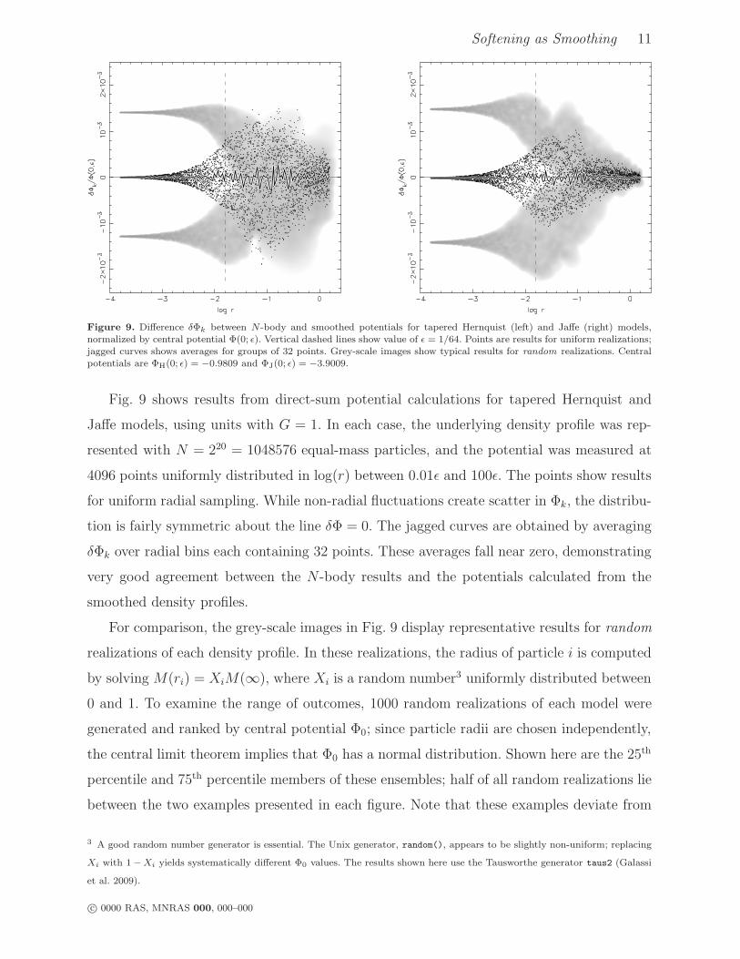
Figure 10. Distribution functions for tapered Hernquist (left) and Ja!e (right) models. Solid curve: f(E); dashed, dot-dashed,and dotted curves: f(E; ") for " = 1/256, 1/64, and 1/16, respectively.
f(E; %) =1$8"2
d
dE
! 0
Ed! (!! E)%1/2 d#
d!. (21)
Note that in d#/d!, the quantity # = #(r) is the underlying density, while ! = !(r; %) is
the smoothed potential, related by Poisson’s equation to the smoothed density #(r; %). In
e"ect, the smoothed potential !(r; %) is taken as a given, and (21) is used to find what will
hereafter be called the smoothed distribution function f(E; %); with this DF, the underlying
profile #(r) is in equilibrium in the adopted potential (e.g., McMillan & Dehnen 2007; Barnes
& Hibbard 2009). Conversely, setting % = 0 yields the self-consistent distribution function
f(E) which describes a self-gravitating model with the underlying profile #(r).
Fig. 10 presents DFs for tapered Hernquist and Ja"e models. In each case the solid line
shows the self-consistent DF; these match the published DFs (Ja"e 1983; Hernquist 1990)
over almost the entire energy range, deviating only for E >) !GM/b = !0.01 where tapering
sets in.
Smoothed DFs for Ja"e models appear very di"erent from their self-consistent counter-
part. The latter has a logarithmic, infinitely deep potential well, which e"ectively confines
material with constant velocity dispersion in a # & r%2 cusp. The characteristic phase-space
density f ) #)%3 & r%2 diverges as r ' 0 (ie, as E ' !(), but only because # does. With
% > 0 the potential well is harmonic at small r, and can’t confine a # & r%2 cusp unless
the local velocity dispersion scales as ) & r; thus the phase-space density now diverges as
f & r%5. Moreover, the domain of f(E; %) is limited to to E0 , E , 0, where E0 % !(0; %).
Thus, instead of growing exponentially as a function of !E, the smoothed DF abruptly
diverges at some finite energy.
By comparison, smoothed DFs for Hernquist models look similar to the self-consistent
DF. The latter has a potential well of finite depth, and the smoothed profiles generate wells
which are only slightly shallower. As the left panel of Fig. 10 shows, all the DFs asymptote to
( as E ' E0. However, the run of velocity dispersion with r is di"erent; the self-consistent
c! 0000 RAS, MNRAS 000, 000–000

14 J. E. Barnes
model has ) & r1/2, implying f & #)%3 & r%5/2. In contrast, the smoothed models have
) & r, implying f & r%4.
One consequence is that the way in which f ' ( as E ' E0 is di"erent in the smoothed
and self-consistent Hernquist models. The self-consistent model has a linear potential as
small r, and thus f & r%5/2 & (E !E0)%5/2. By comparison, the models based on smoothed
potentials have harmonic cores, and as a result, f & r%4 & (E ! E0)%2. (This di"erence is
not apparent in Fig. 10 but becomes obvious when log(E ! E0) is plotted against log f .)
In this respect, the use of a smoothed potential e"ects a non-trivial change on Hernquist
models: f is a di"erent power-law of (E ! E0). Coincidentally, the smoothed Ja"e models
have f & r%5 & (E ! E0)%5/2, just like the self-consistent Hernquist model.
4.3 Dynamical tests
N -body simulations are useful to show that the distribution functions just constructed are
actually in dynamical equilibrium with their smoothed potentials. For each model and %
value, two ensembles of three random realizations were run. In one ensemble, the initial
conditions were generated using the self-consistent DF f(E). The other ensemble used initial
conditions generated from the smoothed DF f(E; %), which allows for the e"ects of softening.
Each realization contained N = 218 = 262144 equal-mass particles. Initial particle radii
ri were selected randomly by solving M(ri) = XiM(() as described above. Initial particle
speeds vi were selected randomly by rejection sampling (von Neumann 1951) from the dis-
tributions g(v; ri) = v2f(12v
2 + !(ri)) or g(v; ri) = v2f(12v
2 + !(ri; %); %), where the former
assumes the self-consistent DF, and the latter a smoothed DF. Position and velocity vectors
for particle i are obtained by multiplying ri and vi by independent unit vectors drawn from
an isotropic distribution. In e"ect, this procedure treats the 6-D distribution function f(r,v)
as a probability density, and selects each particle’s coordinates independently.
Simulations were run using a hierarchical N -body code5. An opening angle of ( = 0.8,
together with quadrupole moments, provided forces with median errors $a/|a|<) 0.0006.
Particles within r ) 10% have much larger force errors, although these seem to have limited
e"ect in practice (Appendix B). Trajectories were integrated using a time-centered leap-frog,
with the same time-step $t = 1/1024 for all particles (see § 4.3.1). All simulations were run
to t = 16, which is more than su%cient to test initial equilibrium.
5 See http://www.ifa.hawaii.edu/faculty/barnes/treecode/treeguide.html for a description.
c! 0000 RAS, MNRAS 000, 000–000

Softening as Smoothing 15
Figure 11. Evolution of potential well depth for N-body simulations of Hernquist (top row) and Ja!e (bottom row) models,each run with the " value labeled. Solid (dotted) curves show results for initial conditions generated from smoothed (self-consistent) DFs. Light grey bands show expected ±2& variation in central potential for N = 262144 independent particles.
Fig. 11 shows how the potential well depth !min of each simulation evolves as a function
of time. Here, well depth is estimated by computing the softened gravitational potential
!i of each particle i and taking the minimum (most negative) value. (This is more accu-
rate than evaluating the potential at the origin since the center of the system may wander
slightly during a dynamical simulation.) To better display the observed changes in !min, the
horizontal axis is logarithmic in time.
Most of the ensembles set up without allowing for softening (dotted curves in Fig. 11)
are clearly not in equilibrium. In all three of the Ja"e models (bottom row), the potential
wells become dramatically shallower on a time-scale comparable to the dynamical time at
r = %. The reason for this is evident. The self-consistent Ja"e model has a central potential
diverging like log r as r ' 0; this potential can confine particles with finite velocity dispersion
at arbitrarily small radii. However, the relatively shallow potential well of a smoothed Ja"e
model cannot confine these particles; they travel outward in a coherent surge and phase-mix
at radii of a few %. Their outward surge and subsequent fallback accounts for the rapid rise
c! 0000 RAS, MNRAS 000, 000–000

16 J. E. Barnes
Figure 12. Density profiles of Ja!e models before and after dynamical evolution. Initial conditions were constructed usingself-consistent DFs (left) and smoothed DFs (right). In each panel, the top profile shows the initial conditions; the smooth curveis the underlying tapered model, overplotted by three slightly bumpy curves showing numerical results from three independentrealizations. The three profiles below show numerical results at t = 16 for simulations run with " = 1/256, 1/64, and 1/16,respectively; each is displaced downward by one additional unit in log ! for clarity.
and partial rebound of the central potential. Similar although less pronounced evolution
occurs in the Hernquist models (top row) with % = 1/16 and possibly with % = 1/64 as
well. Only the self-consistent Hernquist models run with % = 1/256 appear truly close to
equilibrium.
In contrast, all of the ensembles set up with smoothed DFs (solid curves in Fig. 11) are
close to dynamical equilibrium. In equilibrium, gravitational potentials fluctuate as individ-
ual particles move along their orbits. If particles are uncorrelated, the amplitude of these
fluctuations should be comparable to the amplitude seen in an ensemble of independent
realizations. To check this, 1000 realizations of each model were generated; central gravita-
tional potentials !min were evaluated using the same tree algorithm and parameters used
for the self-consistent simulations. The grey horizontal bands show a range of ±2) around
the average central potential for each model and choice of %. Some of the simulations set up
using smoothed DFs wander slightly beyond the 2) range. However, none of them exhibit
the dramatic evolution seen in the cases set up using self-consistent DFs.
The central potential is relatively insensitive to changes in the mass distribution on
scales r * %. To examine small-scale changes directly, density profiles measured from the
initial conditions were compared to profiles measured at t = 16 time units. These profiles
were derived as follows. First, SPH-style interpolation with an adaptive kernel containing 32
particles was used to estimate the density around each particle. Next, the centroid position
rcent of the 32 highest-density particles was determined. Finally, a set of nested spherical
c! 0000 RAS, MNRAS 000, 000–000

Softening as Smoothing 17
shells, centered on rcent, were constructed; each shell was required to contain at least 16
particles and have an outer radius at least 1.05 times its inner radius.
Fig. 12 summarizes results for Ja"e models, which display the most obvious changes.
The density of each shell is plotted against the average distance from rcent of the particles it
contains. In each panel, the top set of curves compare initial (t = 0) numerical results with
the underlying tapered Ja"e model, always represented by a light grey line. Profiles from
three independent N -body realizations of each model are overplotted. While some scatter
from realization to realization is seen, the measured densities track the underlying profile
throughout the entire range plotted. The outermost point is at ) 107 times the radius of the
innermost one; there are not enough particles to obtain measurements at smaller or larger
radii.
Ranged below the top curves in Fig. 12 are numerical results at t = 16 for softening
lengths % = 1/256, 1/64, and 1/16, each shifted downward by one more unit in log #. Again,
profiles from three independent simulations are overplotted to illustrate run-to-run varia-
tions. Simulations set up using the self-consistent DF (left panel) show significant density
evolution; their initial power-law profiles are rapidly replaced by cores of roughly constant
density inside r <) %. In contrast, simulations set up using smoothed DFs (right panel) follow
the initial profile down to r ) 10%4 (although density evolution occurs on smaller scales).
This shows that a careful set-up procedure can maintain the initial density profile even on
scales much smaller than the softening length.
A similar plot for the Hernquist models confirms that most of these simulations start
close to equilibrium. Hernquist models set up using smoothed DFs don’t appear to evolve
at all, although this statement should be qualified since the profiles of these models can’t
be measured reliably on scales much smaller than r ) 10%2. Models set up using the self-
consistent DF and run with % = 1/16 undergo some density evolution; their profiles fall below
the underlying Hernquist model at r ) %, although they continue rising to the innermost
point measured. Simulations run with % = 1/64 or less display no obvious changes down to
scales of r ) 10%2.
It appears that the Ja"e models set up using smoothed DFs are not completely free
of long-term evolution. The right-hand panel of Fig. 12 shows that the peak density as
measured using a fixed number of particles falls by roughly an order of magnitude by t =
16. Moreover, a close examination of Fig. 11 turns some cases with a gradual decrease
in potential well depth; in the smoothed Ja"e models with % = 1/256, for example, !min
c! 0000 RAS, MNRAS 000, 000–000

18 J. E. Barnes
exhibits an upward trend of ) 0.011 percent per unit time. This evolution may not be due
to any flaw in the initial conditions; the central cusps of such models, which are confined
by very shallow harmonic potentials, are fragile and easily disrupted. There may be more
than one mechanism at work here; the rate of potential evolution appears to be inversely
proportional to particle number N , while the rate of density evolution is independent of N .
A full examination of this matter is beyond the scope of this paper.
4.3.1 Choice of time-step
Selecting the time-step $t for an N -body simulation is a non-trivial problem. While the
choice can usually be justified post-hoc by testing for convergence in a series of experiments
with di"erent time-steps, it’s clearly convenient to be able to estimate an appropriate $t a
priori. A general rule governing such estimates is that the time-step should be smaller than
the shortest dynamical time-scale present in the simulation.
The central density #c = #(0; %) of a smoothed density profile defines one such time-
scale. Within the nearly constant-density core of a smoothed profile, the local orbital period
is tc =,
3"/G#c; this is the shortest orbital period anywhere in the system. Numerical tests
show the leap-frog integrator is well-behaved if $t <) 0.05tc (conversely, it becomes unstable
if $t >) 0.15tc). Among the models simulated here, the Ja"e model with % = 1/256 has the
highest smoothed central density; for this model, #c = #J(0; %) + D0(2)#J(%) = 10440. Given
this density, tc + 0.0300 and $t <) 0.0015.
The time required for a fast-moving particle to cross the core region defines another
time-scale. If !c = !(0; %) is depth of the central potential well, the maximum speed of a
bound particle is$!2!c, and the core crossing time is tx = %/
$!2!c. The smoothed Ja"e
model with % = 1/256 has the deepest potential well. For this model, tests of the leap-frog
with fast-moving particles on radial orbits show that $t , tx + 0.0012 yields good results,
but time-steps a few times longer result in poor energy conservation as particles traverse the
core region. (The relationship between tx and the maximum acceptable time-step $t may
be somewhat model-dependent.)
Thus, for the Ja"e model with % = 1/256, both the local criterion based on tc and the
global criterion based on tx yield similar constraints6 on $t. It’s convenient to round $t
6 Assuming " * a, one can show that tc/tx + 11-
ln(a/") for any smoothed Ja!e model; both criteria yield similar constraints
almost independent of ". For smoothed Hernquist models, on the other hand, tc/tx + 11-
a/"; the constraint based on tx is
generally stricter.
c! 0000 RAS, MNRAS 000, 000–000

Softening as Smoothing 19
down to the next power of two, implying $t = 1/1024. This corresponds to $t + 0.03tc +
0.81tx, which is somewhat conservative but helps insure that non-equilibrium changes will
be accurately followed.
To see if this time-step is reasonable, realizations of this model were simulated with
various values of $t between 1/128 to 1/2048. At the lower end of this range, the e"ects
of an over-large time-step manifest quickly; global energy conservation is violated, and the
measured central potential !min drifts upward over time (even though the initial conditions,
generated from f(E; %), are near equilibrium). With a time-step $t = 1/128, for example;
the potential well becomes ) 3 percent shallower during the first two time-steps, and by
t = 4 its depth has decreased by 18 percent. These simulations also violate global energy
conservation, becoming ) 4.5 percent less bound by t = 4. Integration errors are reduced
– but not entirely eliminated – with a time-step $t = 1/256; by t = 4, the potential well
becomes ) 1.3 percent shallower, while total energy changes by ) 0.4 percent. With a time-
step of $t = 1/512 or less, global energy conservation is essentially perfect, and variations
in !min appear to be driven largely by particle discreteness as opposed to time-step e"ects.
Plots analogous to Fig. 12 show that the simulations with time-steps as large as $t =
1/256 + 0.12tc reproduce the inner cusps of Ja"e models just as well as those with $t =
1/1024. With this time-step, individual particles may not be followed accurately, but their
aggregate distribution is not obviously incorrect. On the other hand, a time-step $t = 1/128
yields density profiles which fall below the initial curves for r <) 0.01.
5 DISCUSSION
Softening and smoothing are mathematically equivalent. While the particular form of soft-
ening adopted in (4) corresponds to smoothing with a Plummer kernel (5), other softening
prescriptions can also be described in terms of smoothing operations (e.g. Dehnen 2001).
There are two conceptual advantages to thinking about softening as a smoothing process
transforming the underlying density field #(r) to the smoothed density field #(r; %). First,
since the gravitational potential !(r; %) is related to #(r; %) by Poisson’s equation, the pow-
erful mathematical machinery of classical potential theory becomes available to analyze po-
tentials in N -body simulations. Second, focusing attention on smoothing makes the source
term for the gravitational field explicit. From this perspective, smoothing is not a property
of the particles, but a separate step introduced to ameliorate 1/r singularities in the po-
c! 0000 RAS, MNRAS 000, 000–000
20 J. E. Barnes
tential. Particle themselves are points rather than extended objects; this insures that their
trajectories are characteristics of (1).
Plummer smoothing converts #n(r) & r%n power-laws to cores. At radii r - % the density
profile is essentially unchanged, while at r * % the density approaches a constant value equal
to the density of the underlying model at r = % times a factor which depends only on n. For
the case n = 1, this factor is unity and #1(r; %) = #1($
r2 + %2) everywhere.
The e"ects of Plummer smoothing on astrophysically-motivated models with power-law
cusps, such as the Ja"e, Hernquist, and NFW profiles, follow for the most part from the
results for pure power-laws. In particular, for %<) a/64, where a is the profile’s scale radius,
the power-law results are essentially ‘grafted’ onto the underlying profile. On the other hand,
for %>) a/16, the inner power-law is erased by smoothing.
Smoothing provides a way to predict the potentials obtained in N -body calculations
to an accuracy limited only by$
N fluctuations. These predictions o"er new and powerful
tests of N -body methodology, exposing subtle systematic e"ects which may be di%cult to
diagnose by other means.
Given an underlying density profile #(r), it’s straightforward to construct an isotropic
distribution function f(E; %) such that #(r) is in equilibrium with the potential generated by
its smoothed counterpart #(r; %). Such distribution functions can be used to generate high-
quality equilibrium initial conditions for N -body simulations; they should be particularly
e"ective when realized with ‘quiet start’ procedures (Debattista & Sellwood 2000). Systems
with shallow central cusps, such as Hernquist and NFW models, may be set up fairly close
to equilibrium without taking softening into account as long as % is not too large. However,
it appears impossible to set up a good N -body realization of a Ja"e model without allowing
for softening.
It’s true that realizations so constructed don’t reproduce the actual dynamics of the
underlying models at small radii (Dehnen 2001, footnote 8); to obtain an equilibrium, the
velocity dispersion is reduced on scales r <) %. But realizations set up without softening pre-
serve neither the dispersion nor the density at small radii, and the initial relaxation of such
a system can’t be calculated a priori but must be simulated numerically. On the whole, it
seems better to get the central density profile right on scales r < %, and know how the central
velocity dispersion profile has been modified. Even if the dynamics are not believable within
r <) %, the ability to localize mass on such scales may be advantageous in modeling dynamics
on larger scales.
c! 0000 RAS, MNRAS 000, 000–000

Softening as Smoothing 21
Mathematica code to tabulate smoothed models is available at
http://www.ifa.hawaii.edu/faculty/barnes/research/smoothing/.
ACKNOWLEDGMENTS
I thank Jun Makino and Lars Hernquist for useful and encouraging comments, and an
anonymous referee for a positive and constructive report. Mathematica rocks.
REFERENCES
Athanassoula, E., Bosma, A., Lambert, J.-C., Makino, J. 1998, ‘Performance and accuracy
of a GRAPE-3 system for collisionless N-body simulations’, MNRAS, 293, 369–380
Athanassoula, E., Fady, E., Lambert, J.-C., Bosma, A. 2000, ‘Optimal softening for force
calculations in collisionless N-body simulations’, MNRAS, 314, 475–488
Barnes, J.E. 1998, ‘Dynamics of Galaxy interactions’, in Galaxies: Interactions and Induced
Star Formation, eds. D. Friedli, L. Martinet, & D. Pfenniger. Berlin, Springer, p. 275–394
Barnes, J. & Hut, P. 1986, ‘A hierarchical O(N log N) force-calculation algorithm’, Nature,
324, 446–449
Barnes, J. & Hut, P. 1989, ‘Error analysis of a tree code’, ApJS, 70, 389–417
Barnes, J.E. & Hibbard, J.E. 2009, ‘IDENTIKIT 1: A modeling tool for interacting disc
galaxies’, AJ, 137, 3071–3090
Debattista, V.P. & Sellwood , J.A. 2000, ‘Constraints from Dynamical Friction on the Dark
Matter Content of Barred Galaxies’, ApJ, 543, 704–721
Dehnen, W. 2001, ‘Towards optimal softening in three-dimensional N -body codes – I.
Minimizing the force error’, MNRAS, 324, 273–291
Dyer, C.C. & Ip, P.S.S. 1993, ‘Softening in N -body simulations of collisionless systems’,
ApJ, 409, 60–67
Eddington, A.S. 1916, ‘The distribution of stars in globular clusters’, MNRAS, 76, 572–585
Hernquist, L. & Barnes, J.E. 1990, ‘Are some N -body algorithms intrinsically less collisional
than others?’, ApJ, 349, 562–569
Galassi, M., Davies, J., Theiler, J., Gough, B., Jungman, G., Alken, P., Booth, M., Rossi,
F. 2009, ‘GNU Scientific Library Reference Manual’, Network Theory Ltd, UK
Hernquist, L.E. 1987, ‘Performance Characteristics of Tree Codes’, ApJS, 64, 715–734
c! 0000 RAS, MNRAS 000, 000–000
22 J. E. Barnes
Hernquist, L.E. 1990, ‘An analytical model for spherical galaxies and bulges’, ApJ, 356,
359–364
Ja"e, W. 1983, ‘A simple model for the distribution of light in spherical galaxies’, MNRAS,
202, 995-999
Kazantzidis, S., Magorrian, J., & Moore, B. 2004, ‘Generating Equilibrium Dark Matter
Halos: Inadequacies of the Local Maxwellian Approximation’, ApJ, 601, 37–46
Klimontovich, Yu. L. 1967, ‘The statistical theory of non-equilibrium processes in a plasma’,
M.I.T. Press, Cambridge, MA.
McMillan, P.J. & Dehnen, W. 2007, ‘Initial conditions for disc galaxies’, MNRAS, 378,
541–550
Merritt, D. 1996, ‘Optimal Smoothing for N-Body Codes’, AJ, 111, 2462–2464
Navarro, J.F., Frenk, C.S., & White, S.D.M. 1996, ‘The Structure of Cold Dark Matter
Halos’, ApJ, 462, 563–575
Plummer, H.C. 1911, ‘On the problem of distribution in globular star clusters’, MNRAS,
71, 460–470
von Neumann, J. 1951, ‘Various techniques used in connection with random digits’, in
Monte Carlo Method, eds. A.S. Householder, G.E. Forsythe, & H.H. Germond. National
Bureau of Standards Applied Mathematics Series 12, U.S. Government Printing O%ce,
Washington, D.C., p. 36–38
Wachlin, F.C. & Carpintero, D.D. 2006, ‘Softened potentials and the multipolar expansion’,
Rev. Mex. Astr. Ap., 42, 251–259
APPENDIX A: APPROXIMATIONS
A.1 Power-law profiles
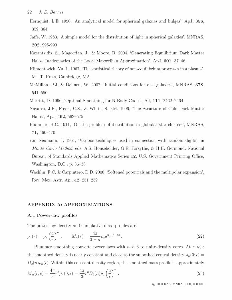
The power-law density and cumulative mass profiles are
#n(r) = #a
%a
r
&n
, Mn(r) =4"
3 ! n#aa
nr(3%n) . (22)
Plummer smoothing converts power laws with n < 3 to finite-density cores. At r * %
the smoothed density is nearly constant and close to the smoothed central density #n(0; %) =
D0(n)#n(%). Within this constant-density region, the smoothed mass profile is approximately
Mn(r; %) =4"
3r3#n(0; %) =
4"
3r3D0(n)#a
%a
%
&n
. (23)
c! 0000 RAS, MNRAS 000, 000–000

Softening as Smoothing 23
Figure 13. Relative error in smoothed density (solid)and mass (dashed) for a ! $ r!1 profile, computed for" = 1 using (25) and (26). Dark curves show results for' = 1.739; light grey solid curves show errors in densityonly for ' = 1.769 (above) and ' = 1.709 (below).
Figure 14. Relative error in smoothed density (solid)and mass (dashed) for a ! $ r!2 profile, computed for" = 1 using (25) and (26). Dark curves show results for' = 1.820; light grey solid curves show errors in densityonly for ' = 1.850 (above) and ' = 1.790 (below).
At r - %, on the other hand, smoothing has little e"ect on the mass profile, so Mn(r; %) +
Mn(r). Interpolating between these functions yields an approximate expression for the
smoothed mass profile:
.Mn(r; %) =#Mn(r; %)%'/n + Mn(r)%'/n
$%n/', (24)
where the shape parameter * determines how abruptly the transition from one function to
the other takes place. This expression can be rearranged to give
.Mn(r; %) =
/
01
3
(3 ! n)D0(n)
2'/n %%
r
&'
+ 1
3
4%n/'
Mn(r) . (25)
The smoothed density profile is obtained by di"erentiating the mass profile:
#̃n(r; %) =1
4"r2
d
dr.Mn(r; %) . (26)
Figs. 13 and 14 present tests of these approximations for # & r%1 and r%2 power-laws,
respectively. As in Figs. 1 and 2, the smoothed density profile was computed with % = 1;
for other values of %, the entire pattern simply shifts left or right without changing shape or
amplitude. Dashed curves show relative errors in smoothed mass, $M = .M(r; %)/M(r; %)!1,
while solid curves are relative errors in smoothed density $! = #̃(r; %)/#(r; %) ! 1. The *
value used for each dark curve is the value which minimizes5
i$!(ri)2 evaluated at points
ri distributed uniformly in log r between log r = !1.5 and 1.5. In light grey, plots of $!(r)
for two other * illustrate the sensitivity to this parameter. Comparing these plots, it appears
that the approximation works better for the # & r%1 power-law than it does for r%2, but
even in the latter case the maximum error is only ) 2%.
Because (25) modifies the underlying mass profile with a multiplicative factor, it can
also be used to approximate e"ects of softening on non-power-law profiles (e.g. Barnes &
Hibbard 2009); for this purpose, both % and * can be treated as free parameters and ad-
c! 0000 RAS, MNRAS 000, 000–000
24 J. E. Barnes
justed to provide a good fit. The resulting errors in density, which amount to a few percent
near the softening scale, are undesirable but don’t appear to seriously compromise N -body
simulations with N ) 105.
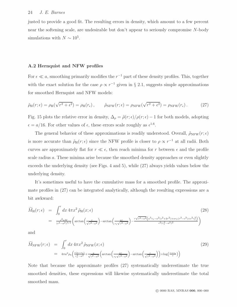
A.2 Hernquist and NFW profiles
For % * a, smoothing primarily modifies the r%1 part of these density profiles. This, together
with the exact solution for the case # & r%1 given in § 2.1, suggests simple approximations
for smoothed Hernquist and NFW models:
#̃H(r; %) = #H($
r2 + %2) = #H(r") , #̃NFW(r; %) = #NFW($
r2 + %2) = #NFW(r") . (27)
Fig. 15 plots the relative error in density, $! = #̃(r; %)/#(r; %)! 1 for both models, adopting
% = a/16. For other values of %, these errors scale roughly as %1.6.
The general behavior of these approximations is readily understood. Overall, #̃NFW(r; %)
is more accurate than #̃H(r; %) since the NFW profile is closer to # & r%1 at all radii. Both
curves are approximately flat for r * %, then reach minima for r between % and the profile
scale radius a. These minima arise because the smoothed density approaches or even slightly
exceeds the underlying density (see Figs. 4 and 5), while (27) always yields values below the
underlying density.
It’s sometimes useful to have the cumulative mass for a smoothed profile. The approxi-
mate profiles in (27) can be integrated analytically, although the resulting expressions are a
bit awkward:
.MH(r; %) =! r
0dx 4"x2 #̃H(x; %) (28)
= !2aM
(!2!a2)3/2
%arctan
#r'
!2!a2
$%arctan
#ar
r!'
!2!a2
$%
r'
!2!a2(a3r!!a2(!2+2r2)+ar!(r2!!2)+!2r2
!)!2(r2
!!a2)2
&
and
.MNFW(r; %) =! r
0dx 4"x2 #̃NFW(x; %) (29)
= 4#a3!a
#r(a!r!)
r2!!a2 + a'
!2!a2
#arctan
#ar
r!'
!2!a2
$%arctan
#r'
!2!a2
$$+log( r+r!
! )$
Note that because the approximate profiles (27) systematically underestimate the true
smoothed densities, these expressions will likewise systematically underestimate the total
smoothed mass.
c! 0000 RAS, MNRAS 000, 000–000
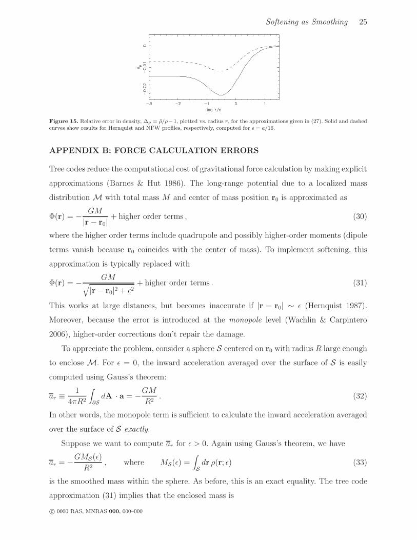
Softening as Smoothing 25
Figure 15. Relative error in density, #" = !̃/!%1, plotted vs. radius r, for the approximations given in (27). Solid and dashedcurves show results for Hernquist and NFW profiles, respectively, computed for " = a/16.
APPENDIX B: FORCE CALCULATION ERRORS
Tree codes reduce the computational cost of gravitational force calculation by making explicit
approximations (Barnes & Hut 1986). The long-range potential due to a localized mass
distribution M with total mass M and center of mass position r0 is approximated as
!(r) = ! GM
|r ! r0|+ higher order terms , (30)
where the higher order terms include quadrupole and possibly higher-order moments (dipole
terms vanish because r0 coincides with the center of mass). To implement softening, this
approximation is typically replaced with
!(r) = ! GM,|r! r0|2 + %2
+ higher order terms . (31)
This works at large distances, but becomes inaccurate if |r ! r0| ) % (Hernquist 1987).
Moreover, because the error is introduced at the monopole level (Wachlin & Carpintero
2006), higher-order corrections don’t repair the damage.
To appreciate the problem, consider a sphere S centered on r0 with radius R large enough
to enclose M. For % = 0, the inward acceleration averaged over the surface of S is easily
computed using Gauss’s theorem:
ar %1
4"R2
!
(SdA · a = !GM
R2. (32)
In other words, the monopole term is su%cient to calculate the inward acceleration averaged
over the surface of S exactly.
Suppose we want to compute ar for % > 0. Again using Gauss’s theorem, we have
ar = !GMS(%)
R2, where MS(%) =
!
Sdr #(r; %) (33)
is the smoothed mass within the sphere. As before, this is an exact equality. The tree code
approximation (31) implies that the enclosed mass is
c! 0000 RAS, MNRAS 000, 000–000
26 J. E. Barnes
M0S(%) =
M
(1 + %2/R2)3/2. (34)
This is correct if M is simply a point mass located at r0. But if M has finite extent, then
the enclosed mass MS(%) is always less than M0S(%). As a result, (31) will systematically
overestimate the inward acceleration and depth of the potential well due to M. Wachlin
& Carpintero (2006) demonstrate a similar result by computing the softened potential of a
homogeneous sphere; they find !GM/,|r ! r0|2 + %2 is only the first term in a series.
The inequality MS(%) < M0S(%) is easily verified for Plummer softening. An analogous
inequality is likely to hold for other smoothing kernels S(r; %) which monotonically decrease
with r. Smoothing kernels with compact support (Dehnen 2001) may be better behaved in
this regard.
Under what conditions are these errors significant? For ‘reasonable’ values of %, most
dynamically relevant interactions are on ranges $r - % where softening has little e"ect;
these interactions are not compromised since (31) is nearly correct at long range. Only if a
significant fraction of a system’s mass lies within a region of size % can these errors become
important. This situation was not investigated in early tree code tests (e.g., Hernquist 1987;
Barnes & Hut 1989), which generally used mass models with cores instead of central cusps,
and even heavily softened Hernquist models don’t have much mass within one softening
radius. On the other hand, Ja"e models pack more mass into small radii; a Ja"e model with
% = a/16 has almost 6 percent of its mass within r = %. Ja"e models should be good test
configurations for examining treecode softening errors.
Tests were run using tapered Ja"e and Hernquist models, realized using the same pa-
rameters (a = 1, b = 100, M = 1, and N = 262144) used in the dynamical experiments
(§ 4.3). In each model, the gravitational field was sampled at 4096 points drawn from the
same distribution as the mass. At each test point, results from the tree code with opening
angle ( = 0.8, including quadrupole terms, were compared with the results of an direct-sum
code. As expected, the tests with Hernquist models showed relatively little trend of force
calculation error with %, although the errors are somewhat larger for % = 1/16 than for
smaller values. In contrast, the tests with Ja"e models reveal a clear relationship between
softening length and force calculation accuracy.
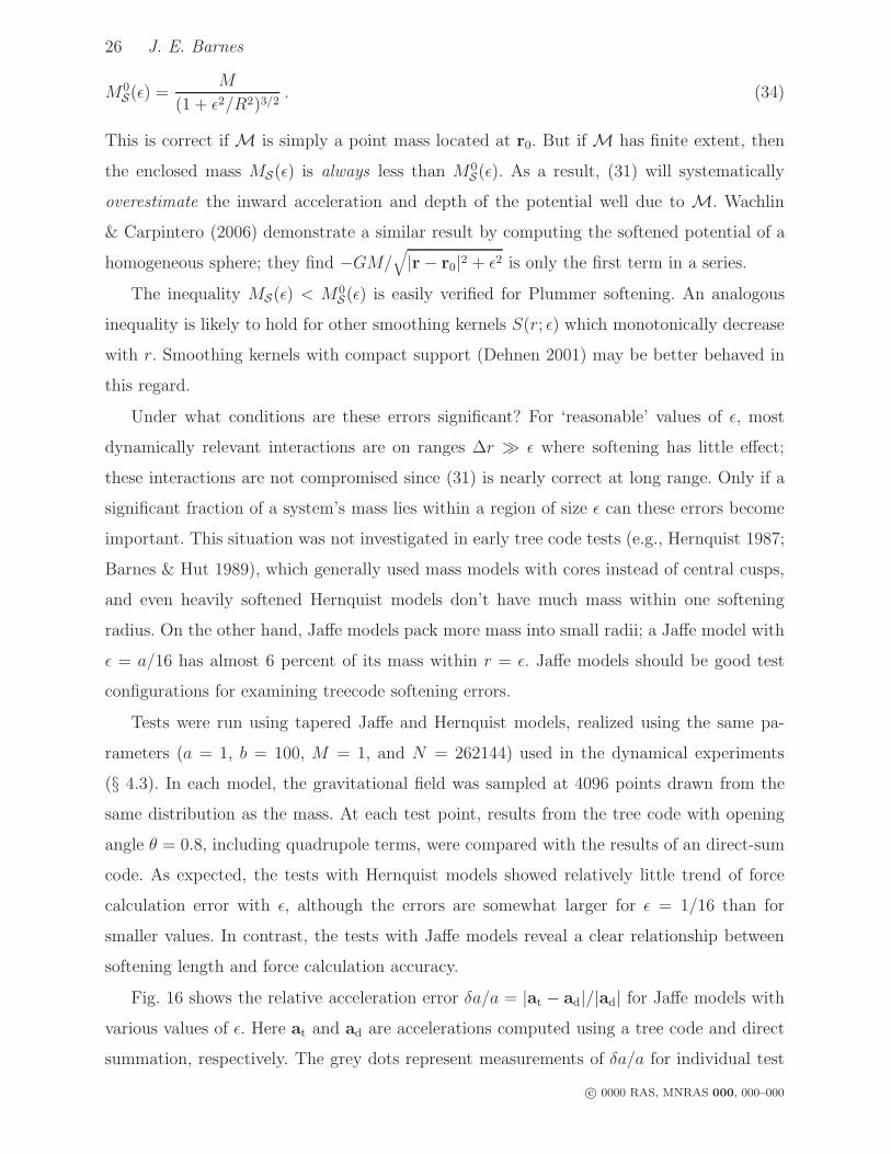
Fig. 16 shows the relative acceleration error $a/a = |at ! ad|/|ad| for Ja"e models with
various values of %. Here at and ad are accelerations computed using a tree code and direct
summation, respectively. The grey dots represent measurements of $a/a for individual test
c! 0000 RAS, MNRAS 000, 000–000

Softening as Smoothing 27
Figure 16. Tree code acceleration error %a/a plottedagainst radius. These results were obtained for a Ja!emodel with ) = 0.8. Grey dots show errors for individualtest points with " = 1/64; the jagged curve threading thedots is constructed by averaging points in groups of 16.Similar curves above and below show results for " = 1/16and " = 1/256, respectively. The large marker on eachcurve shows the average value of %a/a at radius r = ".The light grey curve shows results for " = 0.
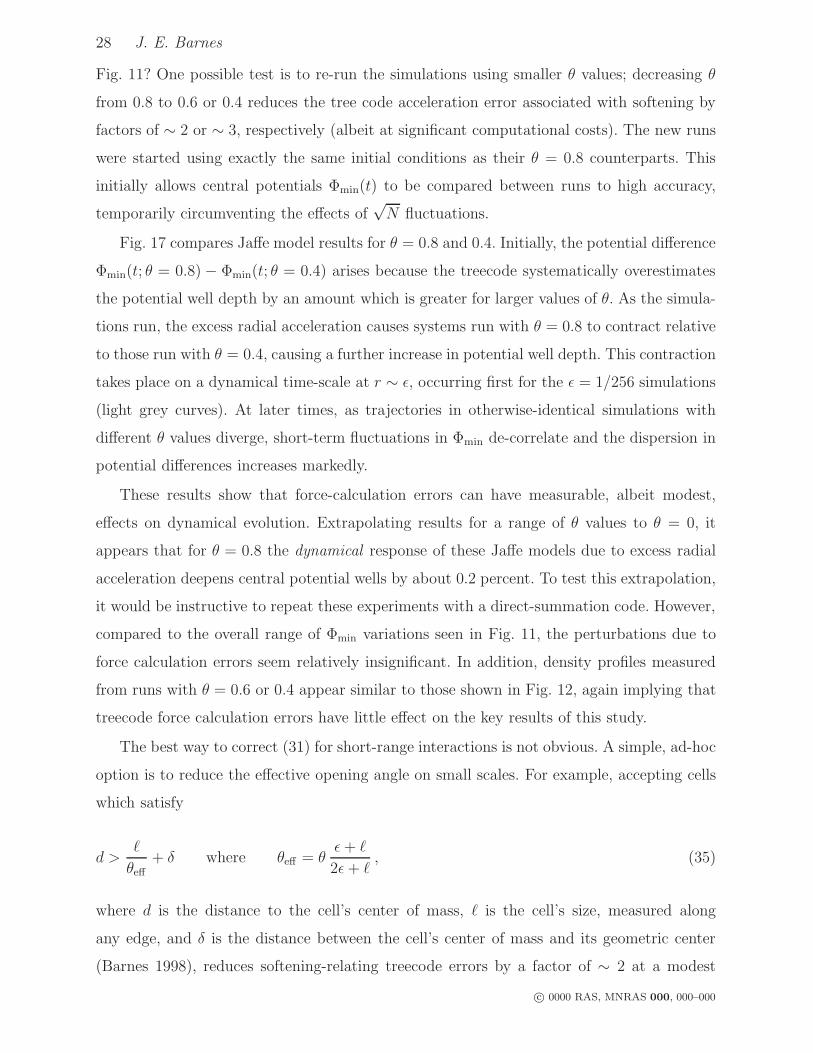
Figure 17. Ja!e model results for evolution of di!erencein potential well depth "min for simulations run with) = 0.8 and 0.4. Light grey, dark grey, and black showpotential di!erences for " = 1/256, 1/64, and 1/16, re-spectively; three independent realizations are plotted ineach case.
points, computed using % = 1/64. The pattern of errors suggests two regimes. At radii
r >) 0.25 (log r >) !0.4), the points fall in a ‘sawtooth’ pattern which reflects the hierarchical
cell structure used in the force calculation. At smaller radii, on the other hand, the relative
error grows more or less monotonically as r ' 0. It appears that errors in the large-r
regime are due to neglect of moments beyond quadrupole order in computing the potentials
of individual cells; conversely, the errors in the small-r regime are due to the tree code’s
inaccurate treatment of softening. The direction of the error vectors at ! ad supports this
interpretation; in the large-r regime they are isotropically distributed, while in the small-r
regime they point toward the center of the system.
The jagged line threading through the dots in Fig. 16, constructed by averaging test
points in groups of 16, shows the overall relationship between acceleration error and radius
for % = 1/64. Similar curves are also plotted for % = 1/16 (above) and % = 1/256 (below).
At large radii, all three curves coincide precisely, implying that force errors are independent
of %. Going to smaller r, the curve for % = 1/16 is the first to diverge, rising above the other
two, next the curve for % = 1/64 begins to rise, tracking the mean distribution of the plotted
dots, and finally the curve for % = 1/256 parallels the other two. Each curve begins rising
monotonically at a radius r ) 20%; this is evidently where softening errors begin to dominate
other errors in the force calculation. At the softening radius r = %, all three curves show
mean acceleration errors $a/a + 0.013.
Are errors of this magnitude dynamically important? In particular, could they explain
some of the potential evolution seen in the runs set up with softening (solid curves) in
c! 0000 RAS, MNRAS 000, 000–000
28 J. E. Barnes
Fig. 11? One possible test is to re-run the simulations using smaller ( values; decreasing (
from 0.8 to 0.6 or 0.4 reduces the tree code acceleration error associated with softening by
factors of ) 2 or ) 3, respectively (albeit at significant computational costs). The new runs
were started using exactly the same initial conditions as their ( = 0.8 counterparts. This
initially allows central potentials !min(t) to be compared between runs to high accuracy,
temporarily circumventing the e"ects of$
N fluctuations.
Fig. 17 compares Ja"e model results for ( = 0.8 and 0.4. Initially, the potential di"erence
!min(t; ( = 0.8) ! !min(t; ( = 0.4) arises because the treecode systematically overestimates
the potential well depth by an amount which is greater for larger values of (. As the simula-
tions run, the excess radial acceleration causes systems run with ( = 0.8 to contract relative
to those run with ( = 0.4, causing a further increase in potential well depth. This contraction
takes place on a dynamical time-scale at r ) %, occurring first for the % = 1/256 simulations
(light grey curves). At later times, as trajectories in otherwise-identical simulations with
di"erent ( values diverge, short-term fluctuations in !min de-correlate and the dispersion in
potential di"erences increases markedly.
These results show that force-calculation errors can have measurable, albeit modest,
e"ects on dynamical evolution. Extrapolating results for a range of ( values to ( = 0, it
appears that for ( = 0.8 the dynamical response of these Ja"e models due to excess radial
acceleration deepens central potential wells by about 0.2 percent. To test this extrapolation,
it would be instructive to repeat these experiments with a direct-summation code. However,
compared to the overall range of !min variations seen in Fig. 11, the perturbations due to
force calculation errors seem relatively insignificant. In addition, density profiles measured
from runs with ( = 0.6 or 0.4 appear similar to those shown in Fig. 12, again implying that
treecode force calculation errors have little e"ect on the key results of this study.
The best way to correct (31) for short-range interactions is not obvious. A simple, ad-hoc
option is to reduce the e"ective opening angle on small scales. For example, accepting cells
which satisfy
d >+
(e!+ $ where (e! = (
% + +
2% + +, (35)
where d is the distance to the cell’s center of mass, + is the cell’s size, measured along
any edge, and $ is the distance between the cell’s center of mass and its geometric center
(Barnes 1998), reduces softening-relating treecode errors by a factor of ) 2 at a modest
c! 0000 RAS, MNRAS 000, 000–000

Softening as Smoothing 29
cost in computing time. Further experiments with similar expressions may produce better
compromises between speed and accuracy.
c! 0000 RAS, MNRAS 000, 000–000