Graphs and Linear Functions - Anna Kuczynska · Graphs and Linear Functions . Graphs of Linear...

section G1 | 101

System of Coordinates, Graphs of Linear Equations and the Midpoint Formula

Graphs and Linear Functions

A 2-dimensional graph is a visual representation of a relationship between two variables given by an equation or an inequality. Graphs help us solve algebraic problems by analysing the geometric aspects of a problem. While equations are more suitable for precise calculations, graphs are more suitable for showing patterns and trends in a relationship. To fully utilize what graphs can offer, we must first understand the concepts and skills involved in graphing that are discussed in this chapter.

G.1 System of Coordinates, Graphs of Linear Equations and the Midpoint Formula

In this section, we will review the rectangular coordinate system, graph various linear equations and inequalities, and introduce a formula for finding coordinates of the midpoint of a given segment.

The Cartesian Coordinate System

A rectangular coordinate system, also called a Cartesian coordinate system (in honor of French mathematician, René Descartes), consists of two perpendicular number lines that cross each other at point zero, called the origin. Traditionally, one of these number lines, usually called the 𝒙𝒙-axis, is positioned horizontally and directed to the right (see Figure 1a). The other number line, usually called 𝒚𝒚-axis, is positioned vertically and directed up. Using this setting, we identify each point 𝑃𝑃 of the plane with an ordered pair of numbers (𝑥𝑥, 𝑦𝑦), which indicates the location of this point with respect to the origin. The first number in the ordered pair, the 𝒙𝒙-coordinate, represents the horizontal distance of the point 𝑃𝑃 from the origin. The second number, the 𝒚𝒚-coordinate, represents the vertical distance of the point 𝑃𝑃 from the origin. For example, to locate point 𝑃𝑃(3,2), we start from the origin, go 3 steps to the right, and then two steps up. To locate point 𝑄𝑄(−3,−2), we start from the origin, go 3 steps to the left, and then two steps down (see Figure 1b). Observe that the coordinates of the origin are (0,0). Also, the second coordinate of any point on the 𝑥𝑥-axis as well as the first coordinate of any point on the 𝑦𝑦-axis is equal to zero. So, points on the 𝑥𝑥-axis have the form (𝑥𝑥, 0), while points on the 𝑦𝑦-axis have the form of (0,𝑦𝑦). To plot (or graph) an ordered pair (𝑥𝑥,𝑦𝑦) means to place a dot at the location given by the ordered pair.

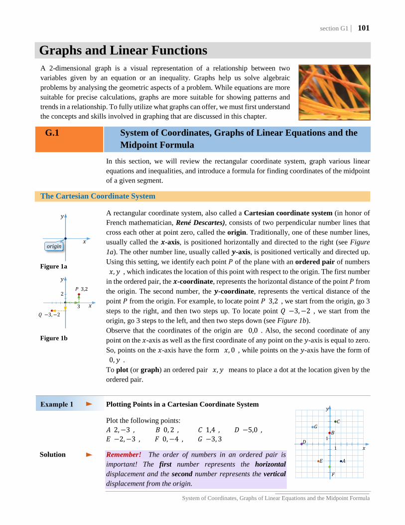
Plotting Points in a Cartesian Coordinate System Plot the following points:

𝐴𝐴(2,−3), 𝐵𝐵(0, 2), 𝐶𝐶(1,4), 𝐷𝐷(−5,0), 𝐸𝐸(−2,−3), 𝐹𝐹(0,−4), 𝐺𝐺(−3, 3) Remember! The order of numbers in an ordered pair is important! The first number represents the horizontal displacement and the second number represents the vertical displacement from the origin.

Solution

𝑦𝑦

𝑥𝑥 origin

𝑦𝑦

𝑥𝑥

𝑃𝑃(3,2)

3 𝑄𝑄(−3,−2)

2

Figure 1a

Figure 1b

𝐹𝐹

𝑦𝑦

𝑥𝑥 1

1 𝐵𝐵

𝐶𝐶

𝐷𝐷

𝐴𝐴 𝐸𝐸

𝐺𝐺

102 | section G1


Graphs of Linear Equations

A graph of an equation in two variables, 𝑥𝑥 and 𝑦𝑦, is the set of points corresponding to all ordered pairs (𝒙𝒙,𝒚𝒚) that satisfy the equation (make the equation true). This means that a graph of an equation is the visual representation of the solution set of this equation.

To determine if a point (𝑎𝑎, 𝑏𝑏) belongs to the graph of a given equation, we check if the equation is satisfied by 𝑥𝑥 = 𝑎𝑎 and 𝑦𝑦 = 𝑏𝑏.

Determining if a Point is a Solution of a Given Equation

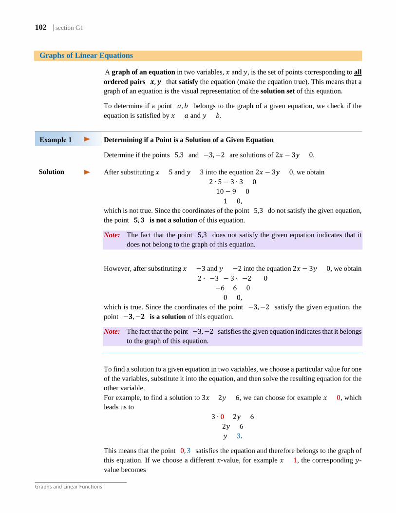
Determine if the points (5,3) and (−3,−2) are solutions of 2𝑥𝑥 − 3𝑦𝑦 = 0. After substituting 𝑥𝑥 = 5 and 𝑦𝑦 = 3 into the equation 2𝑥𝑥 − 3𝑦𝑦 = 0, we obtain

2 ∙ 5 − 3 ∙ 3 = 0 10− 9 = 0

1 = 0, which is not true. Since the coordinates of the point (5,3) do not satisfy the given equation, the point (𝟓𝟓,𝟑𝟑) is not a solution of this equation.

Note: The fact that the point (5,3) does not satisfy the given equation indicates that it does not belong to the graph of this equation.

However, after substituting 𝑥𝑥 = −3 and 𝑦𝑦 = −2 into the equation 2𝑥𝑥 − 3𝑦𝑦 = 0, we obtain 2 ∙ (−3) − 3 ∙ (−2) = 0

−6 + 6 = 0 0 = 0,

which is true. Since the coordinates of the point (−3,−2) satisfy the given equation, the point (−𝟑𝟑,−𝟐𝟐) is a solution of this equation.

Note: The fact that the point (−3,−2) satisfies the given equation indicates that it belongs to the graph of this equation.

To find a solution to a given equation in two variables, we choose a particular value for one of the variables, substitute it into the equation, and then solve the resulting equation for the other variable. For example, to find a solution to 3𝑥𝑥 + 2𝑦𝑦 = 6, we can choose for example 𝑥𝑥 = 0, which leads us to

3 ∙ 0 + 2𝑦𝑦 = 6 2𝑦𝑦 = 6 𝑦𝑦 = 3.

This means that the point (0, 3) satisfies the equation and therefore belongs to the graph of this equation. If we choose a different 𝑥𝑥-value, for example 𝑥𝑥 = 1, the corresponding 𝑦𝑦-value becomes

Solution

section G1 | 103


3 ∙ 1 + 2𝑦𝑦 = 6 2𝑦𝑦 = 3 𝑦𝑦 = 3

2.

So, the point �1, 32� also belongs to the graph.

Since any real number could be selected for the 𝑥𝑥-value, there are infinitely many solutions to this equation. Obviously, we will not be finding all of these infinitely many ordered pairs of numbers in order to graph the solution set to an equation. Rather, based on the location of several solutions that are easy to find, we will look for a pattern and predict the location of the rest of the solutions to complete the graph.

To find more points that belong to the graph of the equation in our example, we might want to solve 3𝑥𝑥 + 2𝑦𝑦 = 6 for 𝑦𝑦. The equation is equivalent to

2𝑦𝑦 = −3𝑥𝑥 + 6

𝑦𝑦 = −32𝑥𝑥 + 3

Observe that if we choose 𝑥𝑥-values to be multiples of 2, the calculations of 𝑦𝑦-values will be easier in this case. Here is a table of a few more (𝑥𝑥,𝑦𝑦) points that belong to the graph:

𝒙𝒙 𝒚𝒚 = −𝟑𝟑𝟐𝟐𝒙𝒙+ 𝟑𝟑 (𝒙𝒙,𝒚𝒚)

−𝟐𝟐 −32(−2) + 3 = 6 (−2, 6)

𝟐𝟐 −32(2) + 3 = 0 (2, 0)

𝟒𝟒 −32(4) + 3 = −3 (4,−3)

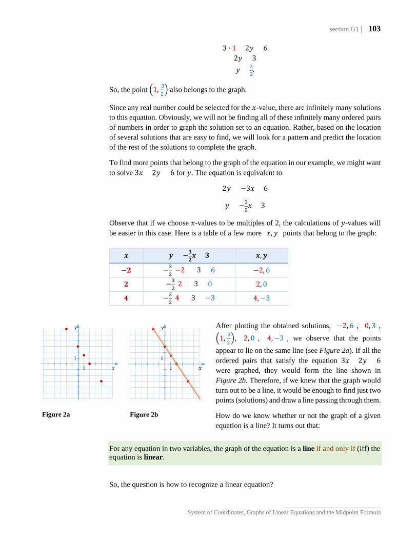
After plotting the obtained solutions, (−2, 6), (0, 3),

�1, 32�, (2, 0), (4,−3), we observe that the points

appear to lie on the same line (see Figure 2a). If all the ordered pairs that satisfy the equation 3𝑥𝑥 + 2𝑦𝑦 = 6 were graphed, they would form the line shown in Figure 2b. Therefore, if we knew that the graph would turn out to be a line, it would be enough to find just two points (solutions) and draw a line passing through them.

How do we know whether or not the graph of a given equation is a line? It turns out that:

For any equation in two variables, the graph of the equation is a line if and only if (iff) the equation is linear.

So, the question is how to recognize a linear equation?

𝑦𝑦

𝑥𝑥 1

1

Figure 2b Figure 2a

𝑦𝑦

𝑥𝑥 1

1

104 | section G1


Definition 1.1 Any equation that can be written in the form

𝑨𝑨𝒙𝒙+ 𝑩𝑩𝒚𝒚 = 𝑪𝑪, where 𝐴𝐴,𝐵𝐵,𝐶𝐶 ∈ ℝ, and 𝐴𝐴 and 𝐵𝐵 are not both 0,

is called a linear equation in two variables.

The form 𝑨𝑨𝒙𝒙 + 𝑩𝑩𝒚𝒚 = 𝑪𝑪 is called standard form of a linear equation.

Graphing Linear Equations Using a Table of Values

Graph 4𝑥𝑥 − 3𝑦𝑦 = 6 using a table of values.

Since this is a linear equation, we expect the graph to be a line. While finding two points satisfying the equation is sufficient to graph a line, it is a good idea to use a third point to guard against errors. To find several solutions, first, let us solve 4𝑥𝑥 − 3𝑦𝑦 = 6 for 𝑦𝑦:

−3𝑦𝑦 = −4𝑥𝑥 + 6 𝑦𝑦 = 4

3𝑥𝑥 − 2

We like to choose 𝑥𝑥-values that will make the calculations of the corresponding 𝑦𝑦-values relatively easy. For example, if 𝑥𝑥 is a multiple of 3, such as −3, 0 or 3, the denominator of 43 will be reduced. Here is the table of points satisfying the given equation and the graph of the line.

To graph a linear equation in standard form, we can develop a table of values as in Example 2, or we can use the 𝑥𝑥- and 𝑦𝑦-intercepts.

Definition 1.2 The 𝒙𝒙-intercept is the point (if any) where the line intersects the 𝑥𝑥-axis. So, the 𝑥𝑥-intercept has the form (𝒙𝒙,𝟎𝟎).

The 𝒚𝒚-intercept is the point (if any) where the line intersects the 𝑦𝑦-axis. So, the 𝑦𝑦-intercept has the form (𝟎𝟎,𝒚𝒚).

Graphing Linear Equations Using 𝒙𝒙- and 𝒚𝒚-intercepts

Graph 5𝑥𝑥 − 3𝑦𝑦 = 15 by finding and plotting the 𝑥𝑥- and 𝑦𝑦-intercepts.

𝒙𝒙 𝒚𝒚 = 𝟒𝟒𝟑𝟑𝒙𝒙 − 𝟐𝟐 (𝒙𝒙,𝒚𝒚)

−𝟑𝟑 43(−3) − 2 = −6 (−3,−6)

𝟎𝟎 43(0)− 2 = −2 (0,−2)

𝟑𝟑 43(3) − 2 = 2 (3, 2)

Solution

𝑦𝑦

𝑥𝑥 −3

2

−6

3

−2

section G1 | 105


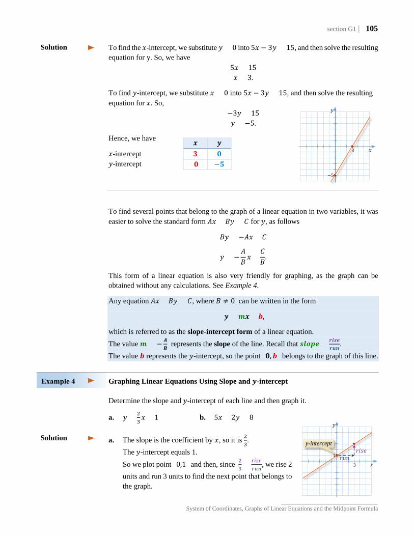
To find the 𝑥𝑥-intercept, we substitute 𝑦𝑦 = 0 into 5𝑥𝑥 − 3𝑦𝑦 = 15, and then solve the resulting equation for y. So, we have

5𝑥𝑥 = 15 𝑥𝑥 = 3.

To find 𝑦𝑦-intercept, we substitute 𝑥𝑥 = 0 into 5𝑥𝑥 − 3𝑦𝑦 = 15, and then solve the resulting equation for 𝑥𝑥. So,

−3𝑦𝑦 = 15 𝑦𝑦 = −5.

Hence, we have

𝑥𝑥-intercept 𝑦𝑦-intercept

To find several points that belong to the graph of a linear equation in two variables, it was easier to solve the standard form 𝐴𝐴𝑥𝑥 + 𝐵𝐵𝑦𝑦 = 𝐶𝐶 for 𝑦𝑦, as follows

𝐵𝐵𝑦𝑦 = −𝐴𝐴𝑥𝑥 + 𝐶𝐶

𝑦𝑦 = −𝐴𝐴𝐵𝐵𝑥𝑥 +

𝐶𝐶𝐵𝐵

.

This form of a linear equation is also very friendly for graphing, as the graph can be obtained without any calculations. See Example 4.

Any equation 𝐴𝐴𝑥𝑥 + 𝐵𝐵𝑦𝑦 = 𝐶𝐶, where 𝐵𝐵 ≠ 0 can be written in the form

𝒚𝒚 = 𝒎𝒎𝒙𝒙 + 𝒃𝒃,

which is referred to as the slope-intercept form of a linear equation. The value 𝒎𝒎 = −𝑨𝑨

𝑩𝑩 represents the slope of the line. Recall that 𝒔𝒔𝒔𝒔𝒔𝒔𝒔𝒔𝒔𝒔 = 𝒓𝒓𝒓𝒓𝒔𝒔𝒔𝒔

𝒓𝒓𝒓𝒓𝒓𝒓.

The value 𝒃𝒃 represents the 𝑦𝑦-intercept, so the point (𝟎𝟎,𝒃𝒃) belongs to the graph of this line.

Graphing Linear Equations Using Slope and 𝒚𝒚-intercept

Determine the slope and 𝑦𝑦-intercept of each line and then graph it.

a. 𝑦𝑦 = 23𝑥𝑥 + 1 b. 5𝑥𝑥 + 2𝑦𝑦 = 8

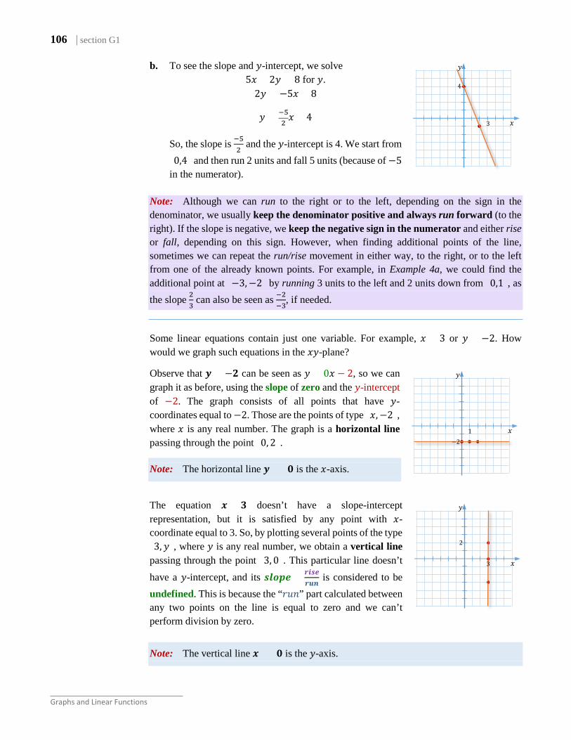
a. The slope is the coefficient by 𝑥𝑥, so it is 2

3.

The 𝑦𝑦-intercept equals 1. So we plot point (0,1) and then, since 2

3= 𝑟𝑟𝑟𝑟𝑟𝑟𝑟𝑟

𝑟𝑟𝑟𝑟𝑟𝑟, we rise 2

units and run 3 units to find the next point that belongs to the graph.

𝒙𝒙 𝒚𝒚 𝟑𝟑 𝟎𝟎 𝟎𝟎 −𝟓𝟓

Solution

Solution

𝑦𝑦

𝑥𝑥

−5

3

1

𝑦𝑦

𝑥𝑥 3

𝑟𝑟𝑟𝑟𝑟𝑟𝑟𝑟 𝑟𝑟𝑟𝑟𝑟𝑟

y-intercept

106 | section G1


b. To see the slope and 𝑦𝑦-intercept, we solve 5𝑥𝑥 + 2𝑦𝑦 = 8 for 𝑦𝑦.

2𝑦𝑦 = −5𝑥𝑥 + 8

𝑦𝑦 = −52𝑥𝑥 + 4

So, the slope is −52

and the 𝑦𝑦-intercept is 4. We start from (0,4) and then run 2 units and fall 5 units (because of −5 in the numerator).

Note: Although we can run to the right or to the left, depending on the sign in the denominator, we usually keep the denominator positive and always run forward (to the right). If the slope is negative, we keep the negative sign in the numerator and either rise or fall, depending on this sign. However, when finding additional points of the line, sometimes we can repeat the run/rise movement in either way, to the right, or to the left from one of the already known points. For example, in Example 4a, we could find the additional point at (−3,−2) by running 3 units to the left and 2 units down from (0,1), as the slope 2

3 can also be seen as −2

−3, if needed.

Some linear equations contain just one variable. For example, 𝑥𝑥 = 3 or 𝑦𝑦 = −2. How would we graph such equations in the 𝑥𝑥𝑦𝑦-plane?

Observe that 𝒚𝒚 = −𝟐𝟐 can be seen as 𝑦𝑦 = 0𝑥𝑥 − 2, so we can graph it as before, using the slope of zero and the 𝑦𝑦-intercept of −2. The graph consists of all points that have 𝑦𝑦-coordinates equal to −2. Those are the points of type (𝑥𝑥,−2), where 𝑥𝑥 is any real number. The graph is a horizontal line passing through the point (0, 2).

Note: The horizontal line 𝒚𝒚 = 𝟎𝟎 is the 𝑥𝑥-axis.

The equation 𝒙𝒙 = 𝟑𝟑 doesn’t have a slope-intercept representation, but it is satisfied by any point with 𝑥𝑥-coordinate equal to 3. So, by plotting several points of the type (3,𝑦𝑦), where 𝑦𝑦 is any real number, we obtain a vertical line passing through the point (3, 0). This particular line doesn’t have a 𝑦𝑦-intercept, and its 𝒔𝒔𝒔𝒔𝒔𝒔𝒔𝒔𝒔𝒔 = 𝒓𝒓𝒓𝒓𝒔𝒔𝒔𝒔

𝒓𝒓𝒓𝒓𝒓𝒓 is considered to be

undefined. This is because the “𝑟𝑟𝑟𝑟𝑟𝑟” part calculated between any two points on the line is equal to zero and we can’t perform division by zero.

Note: The vertical line 𝒙𝒙 = 𝟎𝟎 is the 𝑦𝑦-axis.

𝑦𝑦

𝑥𝑥

4

3

𝑦𝑦

𝑥𝑥 1

−2

𝑦𝑦

𝑥𝑥 3

2

section G1 | 107


In general, the graph of any equation of the type

𝒚𝒚 = 𝒃𝒃, where 𝒃𝒃 ∈ ℝ

is a horizontal line with the 𝑦𝑦-intercept at 𝒃𝒃. The slope of such line is zero.

The graph of any equation of the type 𝒙𝒙 = 𝒂𝒂, where 𝒂𝒂 ∈ ℝ

is a vertical line with the 𝑥𝑥-intercept at 𝒂𝒂. The slope of such line is undefined.

Graphing Special Types of Linear Equations

Graph each equation and state its slope.

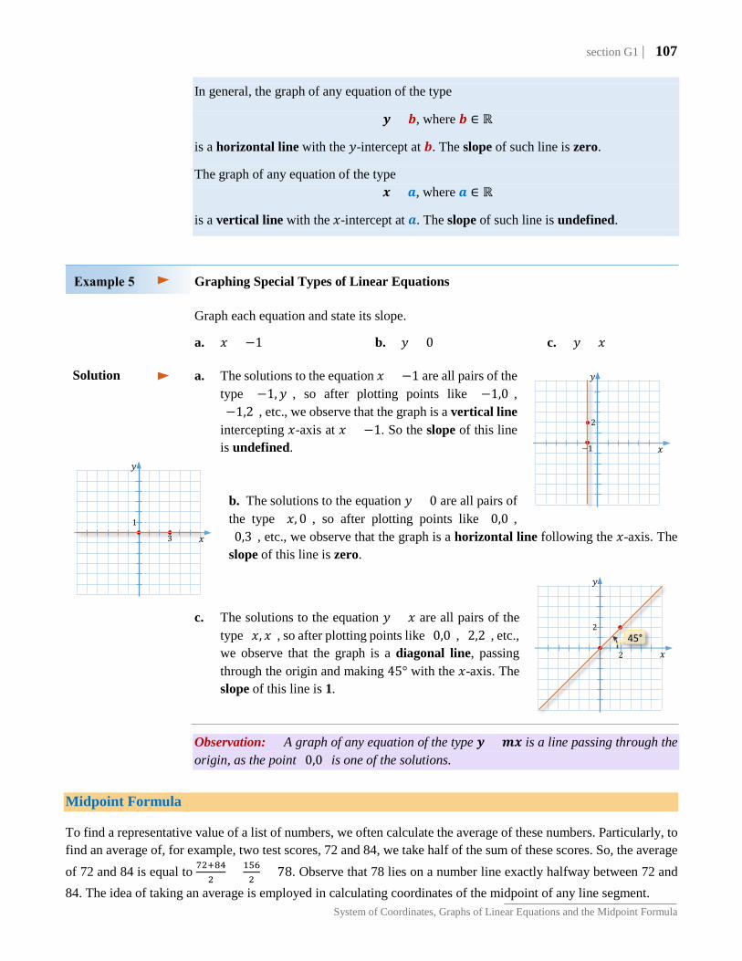
a. 𝑥𝑥 = −1 b. 𝑦𝑦 = 0 c. 𝑦𝑦 = 𝑥𝑥 a. The solutions to the equation 𝑥𝑥 = −1 are all pairs of the

type (−1,𝑦𝑦), so after plotting points like (−1,0), (−1,2), etc., we observe that the graph is a vertical line intercepting 𝑥𝑥-axis at 𝑥𝑥 = −1. So the slope of this line is undefined.

b. The solutions to the equation 𝑦𝑦 = 0 are all pairs of the type (𝑥𝑥, 0), so after plotting points like (0,0), (0,3), etc., we observe that the graph is a horizontal line following the 𝑥𝑥-axis. The slope of this line is zero.

c. The solutions to the equation 𝑦𝑦 = 𝑥𝑥 are all pairs of the type (𝑥𝑥, 𝑥𝑥), so after plotting points like (0,0), (2,2), etc., we observe that the graph is a diagonal line, passing through the origin and making 45° with the 𝑥𝑥-axis. The slope of this line is 1.

Observation: A graph of any equation of the type 𝒚𝒚 = 𝒎𝒎𝒙𝒙 is a line passing through the origin, as the point (0,0) is one of the solutions.

Midpoint Formula To find a representative value of a list of numbers, we often calculate the average of these numbers. Particularly, to find an average of, for example, two test scores, 72 and 84, we take half of the sum of these scores. So, the average of 72 and 84 is equal to 72+84

2= 156

2= 78. Observe that 78 lies on a number line exactly halfway between 72 and

84. The idea of taking an average is employed in calculating coordinates of the midpoint of any line segment.

Solution

𝑦𝑦

𝑥𝑥 3

1

𝑦𝑦

𝑥𝑥 −1

2

𝑦𝑦

𝑥𝑥

2

2

45°

108 | section G1


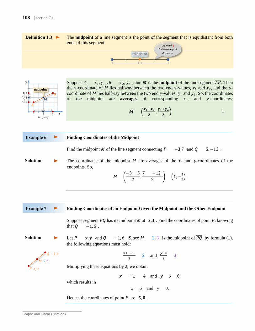
Definition 1.3 The midpoint of a line segment is the point of the segment that is equidistant from both ends of this segment.

Suppose 𝐴𝐴 = (𝑥𝑥1,𝑦𝑦1),𝐵𝐵 = (𝑥𝑥2,𝑦𝑦2), and 𝑴𝑴 is the midpoint of the line segment 𝐴𝐴𝐵𝐵��. Then the 𝑥𝑥-coordinate of 𝑀𝑀 lies halfway between the two end 𝑥𝑥-values, 𝑥𝑥1 and 𝑥𝑥2, and the 𝑦𝑦-coordinate of 𝑀𝑀 lies halfway between the two end 𝑦𝑦-values, 𝑦𝑦1 and 𝑦𝑦2. So, the coordinates of the midpoint are averages of corresponding 𝑥𝑥-, and 𝑦𝑦-coordinates:

𝑴𝑴 = �𝒙𝒙𝟏𝟏+𝒙𝒙𝟐𝟐𝟐𝟐

, 𝒚𝒚𝟏𝟏+𝒚𝒚𝟐𝟐𝟐𝟐

�

Finding Coordinates of the Midpoint

Find the midpoint 𝑀𝑀 of the line segment connecting 𝑃𝑃 = (−3,7) and 𝑄𝑄 = (5,−12). The coordinates of the midpoint 𝑀𝑀 are averages of the 𝑥𝑥- and 𝑦𝑦-coordinates of the endpoints. So,

𝑀𝑀 = �−3 + 5

2,7 + (−12)

2 � = �𝟏𝟏,−𝟓𝟓𝟐𝟐�.

Finding Coordinates of an Endpoint Given the Midpoint and the Other Endpoint

Suppose segment 𝑃𝑃𝑄𝑄 has its midpoint 𝑀𝑀 at (2,3). Find the coordinates of point 𝑃𝑃, knowing that 𝑄𝑄 = (−1, 6).

Let 𝑃𝑃 = (𝑥𝑥,𝑦𝑦) and 𝑄𝑄 = (−1, 6). Since 𝑀𝑀 = (2, 3) is the midpoint of 𝑃𝑃𝑄𝑄��, by formula (1), the following equations must hold:

𝑥𝑥+(−1)2

= 2 and 𝑦𝑦+62

= 3

Multiplying these equations by 2, we obtain

𝑥𝑥 + (−1) = 4 and 𝑦𝑦 + 6 = 6, which results in

𝑥𝑥 = 5 and 𝑦𝑦 = 0.

Hence, the coordinates of point 𝑃𝑃 are (𝟓𝟓,𝟎𝟎).

Solution

Solution

halfway

halfway

𝑨𝑨

𝑦𝑦

𝑥𝑥

2

3

4

3

5 1

midpoint 𝑩𝑩

𝑴𝑴

midpoint

the mark | indicates equal

distances

(1)

𝑃𝑃(𝑥𝑥, 𝑦𝑦)

𝑄𝑄(−1,6)

𝑀𝑀(2,3)

section G1 | 109


G.1 Exercises

Vocabulary Check Fill in each blank with the most appropriate term or phrase from the given list: averages,

graph, horizontal, linear, line, ordered, origin, root, slope, slope-intercept, solution, undefined, vertical, x, x-axis, x-intercept, y, y-axis, y-intercept, zero.

1. The point with coordinates (0, 0) is called the ____________ of a rectangular coordinate system.

2. Each point 𝑃𝑃 of a plane in a rectangular coordinate system is identified with an ___________ pair of numbers (𝑥𝑥,𝑦𝑦), where 𝑥𝑥 measures the _____________ displacement of the point 𝑃𝑃 from the origin and 𝑦𝑦 measures the _____________ displacement of the point 𝑃𝑃 from the origin.

3. Any point on the _____________ has the 𝑥𝑥-coordinate equal to 0.

4. Any point on the _____________ has the 𝑦𝑦-coordinate equal to 0.

5. A ____________ of an equation consists of all points (𝑥𝑥,𝑦𝑦) satisfying the equation.

6. To find the 𝑥𝑥-intercept of a line, we let _____ equal 0 and solve for _____. To find the 𝑦𝑦-intercept, we let _____ equal 0 and solve for _____.

7. Any equation of the form 𝐴𝐴𝑥𝑥 + 𝐵𝐵𝑦𝑦 = 𝐶𝐶, where 𝐴𝐴,𝐵𝐵,𝐶𝐶 ∈ ℝ, and 𝐴𝐴 and 𝐵𝐵 are not both 0, is called a __________ equation in two variables. The graph of such equation is a ________ .

8. In the _______________ form of a line, 𝑦𝑦 = 𝑚𝑚𝑥𝑥 + 𝑏𝑏, the coefficient 𝑚𝑚 represents the _______ and the free term 𝑏𝑏 represents the ______________ of this line.

9. The slope of a vertical line is ______________ and the slope of a horizontal line is _________ .

10. A point where the graph of an equation crosses the 𝑥𝑥-axis is called the _____________ of this graph. This point is also refered to as the ________ or ____________ of the equation.

11. The coordinates of the midpoint of a line segment are the _____________ of the 𝑥𝑥- and 𝑦𝑦-coordinates of the endpoints of this segment.

Concept Check

12. Plot each point in a rectangular coordinate system.

a. (1,2) b. (−2,0) c. (0,−3) d. (4,−1) e. (−1,−3)

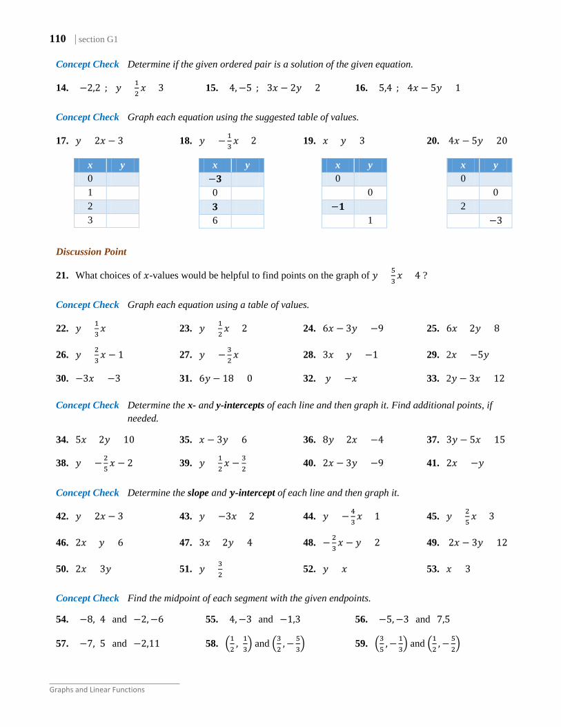
13. State the coordinates of each plotted point.

𝑦𝑦

𝑥𝑥 1

1

𝐵𝐵

𝐶𝐶 𝐷𝐷

𝐴𝐴

𝐸𝐸

𝐺𝐺

𝐹𝐹

110 | section G1


Concept Check Determine if the given ordered pair is a solution of the given equation.

14. (−2,2); 𝑦𝑦 = 12𝑥𝑥 + 3 15. (4,−5); 3𝑥𝑥 − 2𝑦𝑦 = 2 16. (5,4); 4𝑥𝑥 − 5𝑦𝑦 = 1

Concept Check Graph each equation using the suggested table of values.

17. 𝑦𝑦 = 2𝑥𝑥 − 3 18. 𝑦𝑦 = −13𝑥𝑥 + 2 19. 𝑥𝑥 + 𝑦𝑦 = 3 20. 4𝑥𝑥 − 5𝑦𝑦 = 20

Discussion Point

21. What choices of 𝑥𝑥-values would be helpful to find points on the graph of 𝑦𝑦 = 53𝑥𝑥 + 4 ?

Concept Check Graph each equation using a table of values.

22. 𝑦𝑦 = 13𝑥𝑥 23. 𝑦𝑦 = 1

2𝑥𝑥 + 2 24. 6𝑥𝑥 − 3𝑦𝑦 = −9 25. 6𝑥𝑥 + 2𝑦𝑦 = 8

26. 𝑦𝑦 = 23𝑥𝑥 − 1 27. 𝑦𝑦 = −3

2𝑥𝑥 28. 3𝑥𝑥 + 𝑦𝑦 = −1 29. 2𝑥𝑥 = −5𝑦𝑦

30. −3𝑥𝑥 = −3 31. 6𝑦𝑦 − 18 = 0 32. 𝑦𝑦 = −𝑥𝑥 33. 2𝑦𝑦 − 3𝑥𝑥 = 12 Concept Check Determine the x- and y-intercepts of each line and then graph it. Find additional points, if

needed.

34. 5𝑥𝑥 + 2𝑦𝑦 = 10 35. 𝑥𝑥 − 3𝑦𝑦 = 6 36. 8𝑦𝑦 + 2𝑥𝑥 = −4 37. 3𝑦𝑦 − 5𝑥𝑥 = 15

38. 𝑦𝑦 = −25𝑥𝑥 − 2 39. 𝑦𝑦 = 1

2𝑥𝑥 − 3

2 40. 2𝑥𝑥 − 3𝑦𝑦 = −9 41. 2𝑥𝑥 = −𝑦𝑦

Concept Check Determine the slope and 𝒚𝒚-intercept of each line and then graph it.

42. 𝑦𝑦 = 2𝑥𝑥 − 3 43. 𝑦𝑦 = −3𝑥𝑥 + 2 44. 𝑦𝑦 = −43𝑥𝑥 + 1 45. 𝑦𝑦 = 2

5𝑥𝑥 + 3

46. 2𝑥𝑥 + 𝑦𝑦 = 6 47. 3𝑥𝑥 + 2𝑦𝑦 = 4 48. −23𝑥𝑥 − 𝑦𝑦 = 2 49. 2𝑥𝑥 − 3𝑦𝑦 = 12

50. 2𝑥𝑥 = 3𝑦𝑦 51. 𝑦𝑦 = 32 52. 𝑦𝑦 = 𝑥𝑥 53. 𝑥𝑥 = 3

Concept Check Find the midpoint of each segment with the given endpoints.

54. (−8, 4) and (−2,−6) 55. (4,−3) and (−1,3) 56. (−5,−3) and (7,5)

57. (−7, 5) and (−2,11) 58. �12

, 13� and �3

2,−5

3� 59. �3

5,−1

3� and �1

2,−5

2�

x y 0 1 2 3

x y −𝟑𝟑 0 𝟑𝟑 6

x y 0 0

−𝟏𝟏 1

x y 0 0

2 −3

section G1 | 111


Analytic Skills Segment PQ has the given coordinates for one endpoint P and for its midpoint M. Find the coordinates of the other endpoint Q.

60. 𝑃𝑃(−3,2), 𝑀𝑀(3,−2) 61. 𝑃𝑃(7, 10), 𝑀𝑀(5,3)

62. 𝑃𝑃(5,−4), 𝑀𝑀(0,6) 63. 𝑃𝑃(−5,−2), 𝑀𝑀(−1,4)

112 | section G2


G.2 Slope of a Line and Its Interpretation

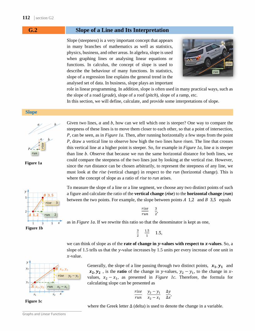
Slope (steepness) is a very important concept that appears in many branches of mathematics as well as statistics, physics, business, and other areas. In algebra, slope is used when graphing lines or analysing linear equations or functions. In calculus, the concept of slope is used to describe the behaviour of many functions. In statistics, slope of a regression line explains the general trend in the analysed set of data. In business, slope plays an important role in linear programming. In addition, slope is often used in many practical ways, such as the slope of a road (grade), slope of a roof (pitch), slope of a ramp, etc. In this section, we will define, calculate, and provide some interpretations of slope.

Slope

Given two lines, 𝑎𝑎 and 𝑏𝑏, how can we tell which one is steeper? One way to compare the steepness of these lines is to move them closer to each other, so that a point of intersection, 𝑃𝑃, can be seen, as in Figure 1a. Then, after running horizontally a few steps from the point 𝑃𝑃, draw a vertical line to observe how high the two lines have risen. The line that crosses this vertical line at a higher point is steeper. So, for example in Figure 1a, line 𝑎𝑎 is steeper than line 𝑏𝑏. Observe that because we run the same horizontal distance for both lines, we could compare the steepness of the two lines just by looking at the vertical rise. However, since the run distance can be chosen arbitrarily, to represent the steepness of any line, we must look at the rise (vertical change) in respect to the run (horizontal change). This is where the concept of slope as a ratio of rise to run arises.

To measure the slope of a line or a line segment, we choose any two distinct points of such a figure and calculate the ratio of the vertical change (rise) to the horizontal change (run) between the two points. For example, the slope between points 𝐴𝐴(1,2) and 𝐵𝐵(3,5) equals

𝑟𝑟𝑟𝑟𝑟𝑟𝑟𝑟𝑟𝑟𝑟𝑟𝑟𝑟

= 32,

as in Figure 1a. If we rewrite this ratio so that the denominator is kept as one,

32

= 1.51

= 1.5,

we can think of slope as of the rate of change in 𝒚𝒚-values with respect to 𝒙𝒙-values. So, a slope of 1.5 tells us that the 𝑦𝑦-value increases by 1.5 units per every increase of one unit in 𝑥𝑥-value.

Generally, the slope of a line passing through two distinct points, (𝒙𝒙𝟏𝟏,𝒚𝒚𝟏𝟏) and (𝒙𝒙𝟐𝟐,𝒚𝒚𝟐𝟐), is the ratio of the change in 𝑦𝑦-values, 𝑦𝑦2 − 𝑦𝑦1, to the change in 𝑥𝑥-values, 𝑥𝑥2 − 𝑥𝑥1, as presented in Figure 1c. Therefore, the formula for calculating slope can be presented as

𝑟𝑟𝑟𝑟𝑟𝑟𝑟𝑟𝑟𝑟𝑟𝑟𝑟𝑟

=𝑦𝑦2 − 𝑦𝑦1𝑥𝑥2 − 𝑥𝑥1

=∆𝑦𝑦∆𝑥𝑥

,

where the Greek letter ∆ (delta) is used to denote the change in a variable.

Figure 1b

Figure 1c

𝑦𝑦

𝑥𝑥

2

3

5

5 1

𝑟𝑟𝑟𝑟𝑟𝑟𝑟𝑟 = 3

𝑩𝑩(𝟑𝟑,𝟓𝟓)

𝑨𝑨(𝟏𝟏,𝟐𝟐) 𝑟𝑟𝑟𝑟𝑟𝑟 = 2

𝑦𝑦

𝑥𝑥

𝑦𝑦1

𝑦𝑦2

𝑥𝑥2 𝑥𝑥1

𝑟𝑟𝑟𝑟𝑟𝑟𝑟𝑟 = 𝑦𝑦2 − 𝑦𝑦1

𝑩𝑩(𝑥𝑥1, 𝑦𝑦2)

𝑨𝑨(𝑥𝑥1, 𝑦𝑦2) 𝑟𝑟𝑟𝑟𝑟𝑟 = 𝑥𝑥2 − 𝑥𝑥1

𝑎𝑎 𝑏𝑏

Figure 1a

𝑎𝑎 𝑏𝑏

𝑟𝑟𝑟𝑟𝑟𝑟

𝑟𝑟𝑟𝑟𝑟𝑟𝑟𝑟

𝑃𝑃

𝑟𝑟𝑟𝑟𝑟𝑟

𝑟𝑟𝑟𝑟𝑟𝑟𝑟𝑟

section G2 | 113

Slope of a Line and Its Interpretation

Definition 2.1 Suppose a line passes through two distinct points (𝒙𝒙𝟏𝟏,𝒚𝒚𝟏𝟏) and (𝒙𝒙𝟐𝟐,𝒚𝒚𝟐𝟐).

If 𝑥𝑥1 ≠ 𝑥𝑥2, then the slope of this line, often denoted by 𝒎𝒎, is equal to

If 𝑥𝑥1 = 𝑥𝑥2, then the slope of the line is said to be undefined.

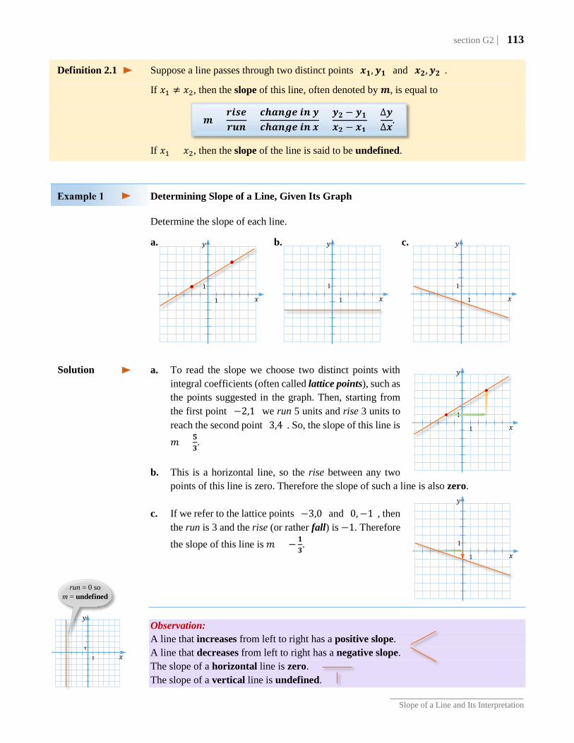
Determining Slope of a Line, Given Its Graph

Determine the slope of each line.

a. b. c. a. To read the slope we choose two distinct points with

integral coefficients (often called lattice points), such as the points suggested in the graph. Then, starting from the first point (−2,1) we run 5 units and rise 3 units to reach the second point (3,4). So, the slope of this line is 𝑚𝑚 = 𝟓𝟓

𝟑𝟑.

b. This is a horizontal line, so the rise between any two

points of this line is zero. Therefore the slope of such a line is also zero. c. If we refer to the lattice points (−3,0) and (0,−1), then

the run is 3 and the rise (or rather fall) is −1. Therefore the slope of this line is 𝑚𝑚 = −𝟏𝟏

𝟑𝟑.

Observation: A line that increases from left to right has a positive slope. A line that decreases from left to right has a negative slope. The slope of a horizontal line is zero. The slope of a vertical line is undefined.

Solution

𝒎𝒎 =𝒓𝒓𝒓𝒓𝒔𝒔𝒔𝒔𝒓𝒓𝒓𝒓𝒓𝒓

=𝒄𝒄𝒄𝒄𝒂𝒂𝒓𝒓𝒄𝒄𝒔𝒔 𝒓𝒓𝒓𝒓 𝒚𝒚𝒄𝒄𝒄𝒄𝒂𝒂𝒓𝒓𝒄𝒄𝒔𝒔 𝒓𝒓𝒓𝒓 𝒙𝒙

=𝒚𝒚𝟐𝟐 − 𝒚𝒚𝟏𝟏𝒙𝒙𝟐𝟐 − 𝒙𝒙𝟏𝟏

=∆𝒚𝒚∆𝒙𝒙

.

𝑦𝑦

𝑥𝑥

1

1

𝑦𝑦

𝑥𝑥

1

1

𝑦𝑦

𝑥𝑥

1

1

𝑦𝑦

𝑥𝑥

1

1

𝑦𝑦

𝑥𝑥

1

1

𝑦𝑦

𝑥𝑥 1

1

run = 0 so m = undefined

114 | section G2


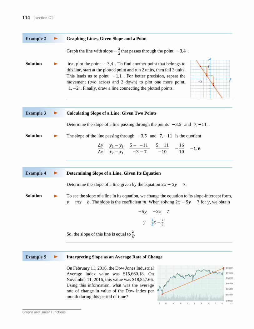
Graphing Lines, Given Slope and a Point

Graph the line with slope −32 that passes through the point (−3,4).

irst, plot the point (−3,4). To find another point that belongs to this line, start at the plotted point and run 2 units, then fall 3 units. This leads us to point (−1,1). For better precision, repeat the movement (two across and 3 down) to plot one more point, (1,−2). Finally, draw a line connecting the plotted points.

Calculating Slope of a Line, Given Two Points

Determine the slope of a line passing through the points (−3,5) and (7,−11).

The slope of the line passing through (−3,5) and (7,−11) is the quotient

∆𝑦𝑦∆𝑥𝑥

=𝑦𝑦2 − 𝑦𝑦1𝑥𝑥2 − 𝑥𝑥1

=5 − (−11)−3− 7

=5 + 11−10

= −1610

= −𝟏𝟏.𝟔𝟔

Determining Slope of a Line, Given Its Equation

Determine the slope of a line given by the equation 2𝑥𝑥 − 5𝑦𝑦 = 7.

To see the slope of a line in its equation, we change the equation to its slope-intercept form, 𝑦𝑦 = 𝑚𝑚𝑥𝑥 + 𝑏𝑏. The slope is the coefficient 𝑚𝑚. When solving 2𝑥𝑥 − 5𝑦𝑦 = 7 for 𝑦𝑦, we obtain

−5𝑦𝑦 = −2𝑥𝑥 + 7

𝑦𝑦 = 𝟐𝟐𝟓𝟓𝑥𝑥 − 7

5.

So, the slope of this line is equal to 𝟐𝟐𝟓𝟓.

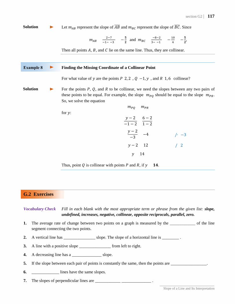
Interpreting Slope as an Average Rate of Change

On February 11, 2016, the Dow Jones Industrial Average index value was $15,660.18. On November 11, 2016, this value was $18,847.66. Using this information, what was the average rate of change in value of the Dow index per month during this period of time?

Solution

Solution

Solution 𝑦𝑦

𝑥𝑥

4

−3

section G2 | 115


The value of the Dow index has increased by 18,847.66− 15,660.18 = 3187.48 dollars over the 9 months (from February 11 to November 11). So, the slope of the line segment connecting the Dow index values on these two days (as marked on the above chart) equals

3187.489

≅ 𝟑𝟑𝟓𝟓𝟒𝟒.𝟏𝟏𝟔𝟔 $/𝑚𝑚𝑚𝑚𝑟𝑟𝑚𝑚ℎ

This means that the value of the Dow index was increasing on average by 354.16 dollars per month between February 11, 2016 and November 11, 2016.

Observe that the change in value was actually different in each month. Sometimes the change was larger than the calculated slope, but sometimes the change was smaller or even negative. However, the slope of the above segment gave us the information about the average rate of change in Dow’s value during the stated period.

Parallel and Perpendicular Lines

Since slope measures the steepness of lines, and parallel lines have the same steepness, then the slopes of parallel lines are equal.

To indicate on a diagram that lines are parallel, we draw on each line arrows pointing in the same direction (see Figure 2). To state in mathematical notation that two lines are parallel, we use the ∥ sign.

To see how the slopes of perpendicular lines are related, rotate a line with a given slope 𝒂𝒂𝒃𝒃

(where 𝑏𝑏 ≠ 0) by 90°, as in Figure 3. Observe that under this rotation the vertical change 𝒂𝒂 becomes the horizontal change but in opposite direction (–𝒂𝒂), and the horizontal change

𝒃𝒃 becomes the vertical change. So, the slope of the perpendicular line is −𝒃𝒃𝒂𝒂. In other

words, slopes of perpendicular lines are opposite reciprocals. Notice that the product of perpendicular slopes, 𝒂𝒂

𝒃𝒃∙ �− 𝒃𝒃

𝒂𝒂�, is equal to −𝟏𝟏.

In the case of 𝑏𝑏 = 0, the slope is undefined, so the line is vertical. After rotation by 90°, we obtain a horizontal line, with a slope of zero. So a line with a zero slope and a line with an “undefined” slope can also be considered perpendicular.

To indicate on a diagram that two lines are perpendicular, we draw a square at the intersection of the two lines, as in Figure 3. To state in mathematical notation that two lines are perpendicular, we use the ⊥ sign. In summary, if 𝒎𝒎𝟏𝟏 and 𝒎𝒎𝟐𝟐 are slopes of two lines, then the lines are:

• parallel iff 𝒎𝒎𝟏𝟏 = 𝒎𝒎𝟐𝟐, and • perpendicular iff 𝒎𝒎𝟏𝟏 = − 𝟏𝟏

𝒎𝒎𝟐𝟐 (or equivalently, if 𝒎𝒎𝟏𝟏 ∙ 𝒎𝒎𝟐𝟐 = −𝟏𝟏)

In addition, a horizontal line (with a slope of zero) is perpendicular to a vertical line (with undefined slope).

Solution

Figure 2

Figure 3

−𝒂𝒂

𝒂𝒂

𝒃𝒃

𝒃𝒃

116 | section G2


Determining Whether the Given Lines are Parallel, Perpendicular, or Neither

For each pair of linear equations, determine whether the lines are parallel, perpendicular, or neither.

a. 3𝑥𝑥 + 5𝑦𝑦 = 75𝑥𝑥 − 3𝑦𝑦 = 4

b. 𝑦𝑦 = 𝑥𝑥 2𝑥𝑥 − 2𝑦𝑦 = 5

c. 𝑦𝑦 = 5 𝑦𝑦 = 5𝑥𝑥

a. As seen in section G1, the slope of a line given by an equation in standard form, 𝐴𝐴𝑥𝑥 +

𝐵𝐵𝑦𝑦 = 𝐶𝐶, is equal to −𝐴𝐴𝐵𝐵

. One could confirm this by solving the equation for 𝑦𝑦 and taking the coefficient by 𝑥𝑥 for the slope.

Using this fact, the slope of the line 3𝑥𝑥 + 5𝑦𝑦 = 7 is −𝟑𝟑𝟓𝟓, and the slope of 5𝑥𝑥 − 3𝑦𝑦 = 4

is 𝟓𝟓𝟑𝟑. Since these two slopes are opposite reciprocals of each other, the two lines are

perpendicular.

b. The slope of the line 𝑦𝑦 = 𝑥𝑥 is 1 and the slope of 2𝑥𝑥 − 2𝑦𝑦 = 5 is also 22

= 𝟏𝟏. So, the two lines are parallel.

c. The line 𝑦𝑦 = 5 can be seen as 𝑦𝑦 = 0𝑥𝑥 + 5, so its slope is 0. The slope of the second line, 𝑦𝑦 = 5𝑥𝑥, is 𝟓𝟓. So, the two lines are neither parallel nor perpendicular.

Collinear Points

Definition 2.2 Points that lie on the same line are called collinear.

Two points are always collinear because there is only one line passing through these points. The question is how could we check if a third point is collinear with the given two points? If we have an equation of the line passing through the first two points, we could plug in the coordinates of the third point and see if the equation is satisfied. If it is, the third point is collinear with the other two. But, can we check if points are collinear without referring to an equation of a line?

Notice that if several points lie on the same line, the slope between any pair of these points will be equal to the slope of this line. So, these slopes will be the same. One can also show that if the slopes between any two points in the group are the same, then such points lie on the same line. So, they are collinear. Points are collinear iff the slope between each pair of points is the same.

Determine Whether the Given Points are Collinear

Determine whether the points 𝐴𝐴(−3,7), 𝐵𝐵(−1,2), and 𝐶𝐶 = (3,−8) are collinear.

Solution

𝐶𝐶

𝐵𝐵 𝐴𝐴

https://www.mathsisfun.com/definitions/collinear.html

section G2 | 117


Let 𝑚𝑚𝐴𝐴𝐵𝐵 represent the slope of 𝐴𝐴𝐵𝐵�� and 𝑚𝑚𝐵𝐵𝐵𝐵 represent the slope of 𝐵𝐵𝐶𝐶��. Since

𝑚𝑚𝐴𝐴𝐵𝐵 = 2−7−1−(−3) = −𝟓𝟓

𝟐𝟐 and 𝑚𝑚𝐵𝐵𝐵𝐵 = −8−2

3−(−1) = −104

= −𝟓𝟓𝟐𝟐,

Then all points 𝐴𝐴, 𝐵𝐵, and 𝐶𝐶 lie on the same line. Thus, they are collinear.

Finding the Missing Coordinate of a Collinear Point

For what value of 𝑦𝑦 are the points 𝑃𝑃(2, 2), 𝑄𝑄(−1,𝑦𝑦), and 𝑅𝑅(1, 6) collinear? For the points 𝑃𝑃, 𝑄𝑄, and 𝑅𝑅 to be collinear, we need the slopes between any two pairs of these points to be equal. For example, the slope 𝑚𝑚𝑃𝑃𝑃𝑃 should be equal to the slope 𝑚𝑚𝑃𝑃𝑃𝑃. So, we solve the equation

𝑚𝑚𝑃𝑃𝑃𝑃 = 𝑚𝑚𝑃𝑃𝑃𝑃 for 𝑦𝑦:

𝑦𝑦 − 2−1− 2

=6 − 21 − 2

𝑦𝑦 − 2−3

= −4

𝑦𝑦 − 2 = 12

𝑦𝑦 = 14 Thus, point 𝑄𝑄 is collinear with points 𝑃𝑃 and 𝑅𝑅, if 𝑦𝑦 = 𝟏𝟏𝟒𝟒.

G.2 Exercises

Vocabulary Check Fill in each blank with the most appropriate term or phrase from the given list: slope,

undefined, increases, negative, collinear, opposite reciprocals, parallel, zero.

1. The average rate of change between two points on a graph is measured by the ____________ of the line segment connecting the two points.

2. A vertical line has _______________ slope. The slope of a horizontal line is ________ .

3. A line with a positive slope _______________ from left to right.

4. A decreasing line has a ______________ slope.

5. If the slope between each pair of points is constantly the same, then the points are _________________.

6. _____________ lines have the same slopes.

7. The slopes of perpendicular lines are ____________ ______________ .

Solution

Solution

/∙ (−3)

/+2

118 | section G2


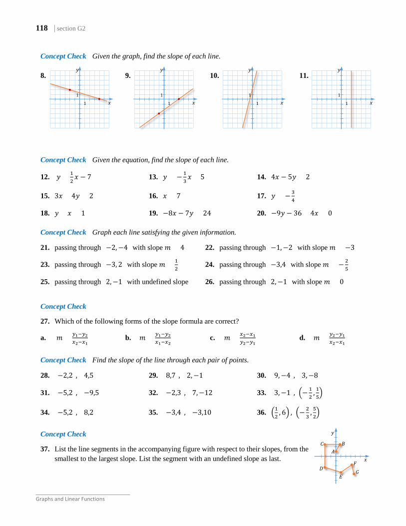
Concept Check Given the graph, find the slope of each line. 8. 9. 10. 11.

Concept Check Given the equation, find the slope of each line.

12. 𝑦𝑦 = 12𝑥𝑥 − 7 13. 𝑦𝑦 = −1

3𝑥𝑥 + 5 14. 4𝑥𝑥 − 5𝑦𝑦 = 2

15. 3𝑥𝑥 + 4𝑦𝑦 = 2 16. 𝑥𝑥 = 7 17. 𝑦𝑦 = −34

18. 𝑦𝑦 + 𝑥𝑥 = 1 19. −8𝑥𝑥 − 7𝑦𝑦 = 24 20. −9𝑦𝑦 − 36 + 4𝑥𝑥 = 0 Concept Check Graph each line satisfying the given information.

21. passing through (−2,−4) with slope 𝑚𝑚 = 4 22. passing through (−1,−2) with slope 𝑚𝑚 = −3

23. passing through (−3, 2) with slope 𝑚𝑚 = 12 24. passing through (−3,4) with slope 𝑚𝑚 = −2

5

25. passing through (2,−1) with undefined slope 26. passing through (2,−1) with slope 𝑚𝑚 = 0

Concept Check

27. Which of the following forms of the slope formula are correct?

a. 𝑚𝑚 = 𝑦𝑦1−𝑦𝑦2𝑥𝑥2−𝑥𝑥1

b. 𝑚𝑚 = 𝑦𝑦1−𝑦𝑦2𝑥𝑥1−𝑥𝑥2

c. 𝑚𝑚 = 𝑥𝑥2−𝑥𝑥1𝑦𝑦2−𝑦𝑦1

d. 𝑚𝑚 = 𝑦𝑦2−𝑦𝑦1𝑥𝑥2−𝑥𝑥1

Concept Check Find the slope of the line through each pair of points.

28. (−2,2), (4,5) 29. (8,7), (2,−1) 30. (9,−4), (3,−8)

31. (−5,2), (−9,5) 32. (−2,3), (7,−12) 33. (3,−1), �− 12

, 15�

34. (−5,2), (8,2) 35. (−3,4), (−3,10) 36. �12

, 6� , �−23

, 52�

Concept Check

37. List the line segments in the accompanying figure with respect to their slopes, from the smallest to the largest slope. List the segment with an undefined slope as last.

𝑦𝑦

𝑥𝑥 1

1

𝑦𝑦

𝑥𝑥 1

1

𝑦𝑦

𝑥𝑥 1

1

𝑦𝑦

𝑥𝑥 1

1

𝐹𝐹

𝐸𝐸

𝑦𝑦

𝑥𝑥 𝐴𝐴

𝐵𝐵

𝐷𝐷

𝐶𝐶

𝐺𝐺

section G2 | 119


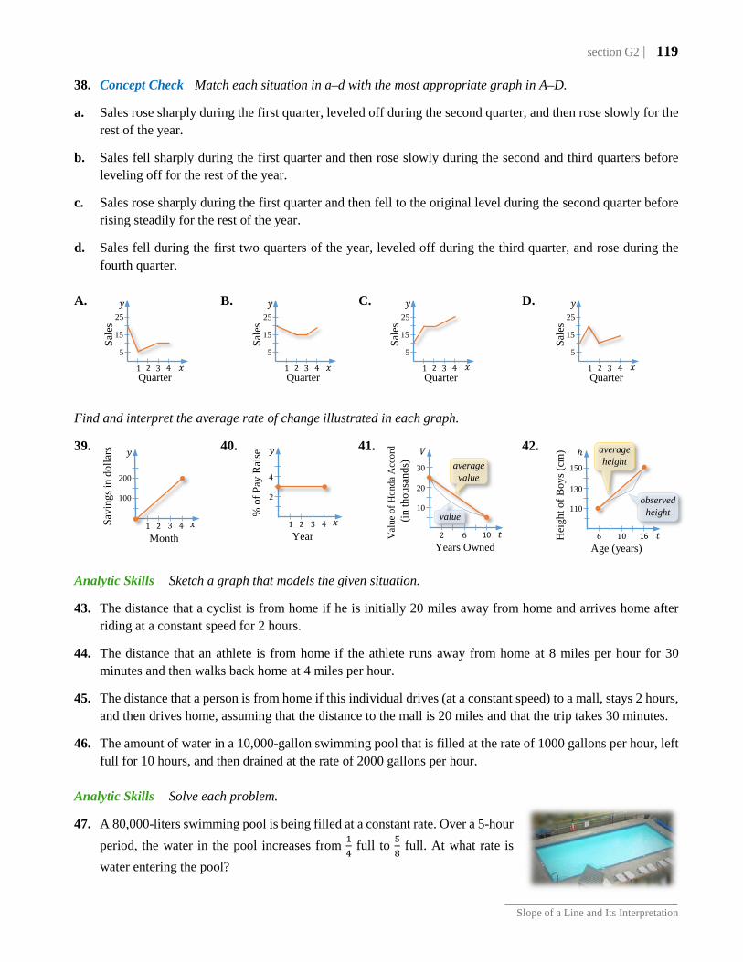
38. Concept Check Match each situation in a–d with the most appropriate graph in A–D.

a. Sales rose sharply during the first quarter, leveled off during the second quarter, and then rose slowly for the rest of the year.

b. Sales fell sharply during the first quarter and then rose slowly during the second and third quarters before leveling off for the rest of the year.

c. Sales rose sharply during the first quarter and then fell to the original level during the second quarter before rising steadily for the rest of the year.

d. Sales fell during the first two quarters of the year, leveled off during the third quarter, and rose during the fourth quarter.

A. B. C. D.

Find and interpret the average rate of change illustrated in each graph.

39. 40. 41. 42.

Analytic Skills Sketch a graph that models the given situation.

43. The distance that a cyclist is from home if he is initially 20 miles away from home and arrives home after riding at a constant speed for 2 hours.

44. The distance that an athlete is from home if the athlete runs away from home at 8 miles per hour for 30 minutes and then walks back home at 4 miles per hour.

45. The distance that a person is from home if this individual drives (at a constant speed) to a mall, stays 2 hours, and then drives home, assuming that the distance to the mall is 20 miles and that the trip takes 30 minutes.

46. The amount of water in a 10,000-gallon swimming pool that is filled at the rate of 1000 gallons per hour, left full for 10 hours, and then drained at the rate of 2000 gallons per hour.

Analytic Skills Solve each problem.

47. A 80,000-liters swimming pool is being filled at a constant rate. Over a 5-hour period, the water in the pool increases from 1

4 full to 5

8 full. At what rate is

water entering the pool?

1 3

𝑦𝑦

𝑥𝑥

5

Quarter

4

Sale

s

2

15

25

1 3

𝑦𝑦

𝑥𝑥

5

Quarter

4

Sale

s

2

15

25

1 3

𝑦𝑦

𝑥𝑥 5

Quarter

4

Sale

s

2

15

25

1 3

𝑦𝑦

𝑥𝑥 5

Quarter

4

Sale

s

2

15

25

1 3

𝑦𝑦

𝑥𝑥

100

Month

4 Savi

ngs i

n do

llars

2

200

1 3

𝑦𝑦

𝑥𝑥

2

Year 4

% o

f Pay

Rai

se

2

4 average

value

2 6

𝑉𝑉

𝑚𝑚

10

Years Owned

Val

ue o

f Hon

da A

ccor

d

(in th

ousa

nds)

10

20

30

value

average height

6 10

ℎ

𝑚𝑚

110

Age (years) H

eigh

t of B

oys (

cm)

16

130

150

observed height

120 | section G2


48. An airplane on a 1,800-kilometer trip is flying at a constant rate. Over a 2-hour period, the location of the plane changes from covering 1

3 of the distance to covering 3

4 of the distance. What is the speed of the airplane?

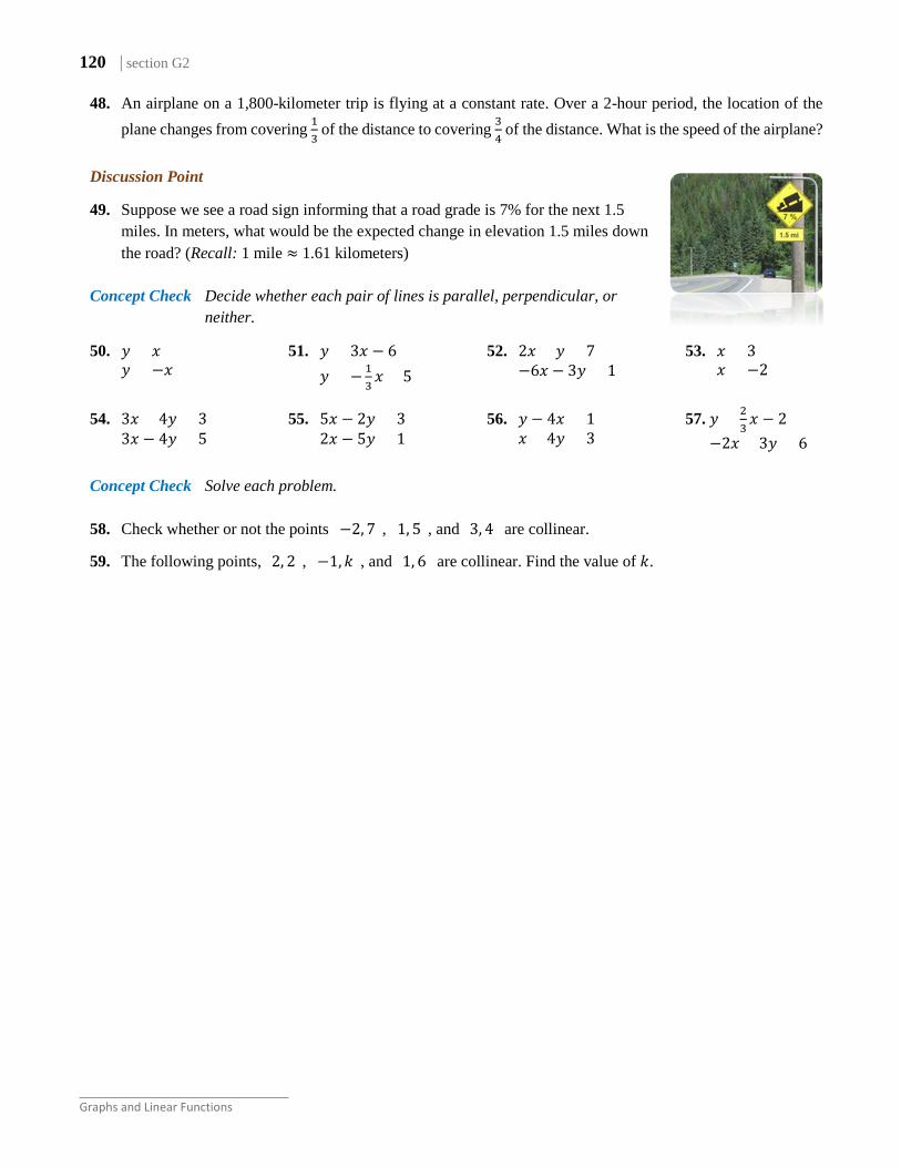
Discussion Point

49. Suppose we see a road sign informing that a road grade is 7% for the next 1.5 miles. In meters, what would be the expected change in elevation 1.5 miles down the road? (Recall: 1 mile ≈ 1.61 kilometers)

Concept Check Decide whether each pair of lines is parallel, perpendicular, or

neither.

50. 𝑦𝑦 = 𝑥𝑥𝑦𝑦 = −𝑥𝑥

51. 𝑦𝑦 = 3𝑥𝑥 − 6𝑦𝑦 = −1

3𝑥𝑥 + 5

52. 2𝑥𝑥 + 𝑦𝑦 = 7−6𝑥𝑥 − 3𝑦𝑦 = 1

53. 𝑥𝑥 = 3𝑥𝑥 = −2

54. 3𝑥𝑥 + 4𝑦𝑦 = 33𝑥𝑥 − 4𝑦𝑦 = 5

55. 5𝑥𝑥 − 2𝑦𝑦 = 32𝑥𝑥 − 5𝑦𝑦 = 1

56. 𝑦𝑦 − 4𝑥𝑥 = 1𝑥𝑥 + 4𝑦𝑦 = 3

57. 𝑦𝑦 = 23𝑥𝑥 − 2

−2𝑥𝑥 + 3𝑦𝑦 = 6

Concept Check Solve each problem. 58. Check whether or not the points (−2, 7), (1, 5), and (3, 4) are collinear.

59. The following points, (2, 2), (−1,𝑘𝑘), and (1, 6) are collinear. Find the value of 𝑘𝑘.

section G3 | 121

Forms of Linear Equations in Two Variables

G.3 Forms of Linear Equations in Two Variables

Linear equations in two variables can take different forms. Some forms are easier to use for graphing, while others are more suitable for finding an equation of a line given two pieces of information. In this section, we will take a closer look at various forms of linear equations and their utilities.

Forms of Linear Equations

The form of a linear equation that is most useful for graphing lines is the slope-intercept form, as introduced in section G1.

Definition 3.1 The slope-intercept form of the equation of a line with slope 𝒎𝒎 and 𝒚𝒚-intercept (0,𝒃𝒃) is

𝒚𝒚 = 𝒎𝒎𝒙𝒙 + 𝒃𝒃.

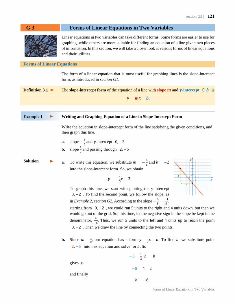
Writing and Graphing Equation of a Line in Slope-Intercept Form Write the equation in slope-intercept form of the line satisfying the given conditions, and

then graph this line.

a. slope −45 and 𝑦𝑦-intercept (0,−2)

b. slope 12 and passing through (2,−5)

a. To write this equation, we substitute 𝑚𝑚 = −4

5 and 𝑏𝑏 = −2

into the slope-intercept form. So, we obtain

𝒚𝒚 = −𝟒𝟒𝟓𝟓𝒙𝒙 − 𝟐𝟐.

To graph this line, we start with plotting the y-intercept (0,−2). To find the second point, we follow the slope, as in Example 2, section G2. According to the slope −4

5= −4

5,

starting from (0,−2), we could run 5 units to the right and 4 units down, but then we would go out of the grid. So, this time, let the negative sign in the slope be kept in the denominator, 4

−5. Thus, we run 5 units to the left and 4 units up to reach the point

(0,−2). Then we draw the line by connecting the two points. b. Since 𝑚𝑚 = 1

2, our equation has a form 𝑦𝑦 = 1

2𝑥𝑥 + 𝑏𝑏. To find 𝑏𝑏, we substitute point (2,−5) into this equation and solve for 𝑏𝑏. So

−5 = 12(2) + 𝑏𝑏

gives us −5 = 1 + 𝑏𝑏

and finally 𝑏𝑏 = −6.

Solution 𝑦𝑦

𝑥𝑥 5

1

−4

1

122 | section G3


Therefore, our equation of the line is 𝒚𝒚 = 𝟏𝟏𝟐𝟐𝒙𝒙 − 𝟔𝟔.

We graph it, starting by plotting the given point (2,−5) and finding the second point by following the slope of 1

2, as

described in Example 2, section G2.

The form of a linear equation that is most useful when writing equations of lines with unknown 𝑦𝑦-intercept is the slope-point form.

Definition 3.2 The slope-point form of the equation of a line with slope 𝒎𝒎 and passing through the point (𝒙𝒙𝟏𝟏,𝒚𝒚𝟏𝟏) is

𝒚𝒚 − 𝒚𝒚𝟏𝟏 = 𝒎𝒎(𝒙𝒙 − 𝒙𝒙𝟏𝟏).

This form is based on the defining property of a line. A line can be defined as a set of points with a constant slope 𝑚𝑚 between any two of these points. So, if (𝑥𝑥1,𝑦𝑦1) is a given (fixed) point of the line and (𝑥𝑥,𝑦𝑦) is any (variable) point of the line, then, since the slope is equal to 𝑚𝑚 for all such points, we can write the equation

𝑚𝑚 =𝑦𝑦 − 𝑦𝑦1𝑥𝑥 − 𝑥𝑥1

.

After multiplying by the denominator, we obtain the slope-point formula, as in Definition 3.2.

Writing Equation of a Line Using Slope-Point Form Use the slope-point form to write an equation of the line satisfying the given conditions.

Leave the answer in the slope-intercept form and then graph the line.

a. slope −23 and passing through (1,−3)

b. passing through points (2, 5) and (−1,−2) a. To write this equation, we plug the slope 𝑚𝑚 = −2

3 and the coordinates of the point

(1,−3) into the slope-point form of a line. So, we obtain

𝑦𝑦 − (−3) = −23(𝑥𝑥 − 1)

𝑦𝑦 + 3 = −23𝑥𝑥 + 2

3

𝑦𝑦 = −23𝑥𝑥 + 2

3− 9

3

𝒚𝒚 = −𝟐𝟐𝟑𝟑𝒙𝒙 − 𝟕𝟕

𝟑𝟑

𝑦𝑦

𝑥𝑥

1

1

2

1

Solution

/−3

section G3 | 123


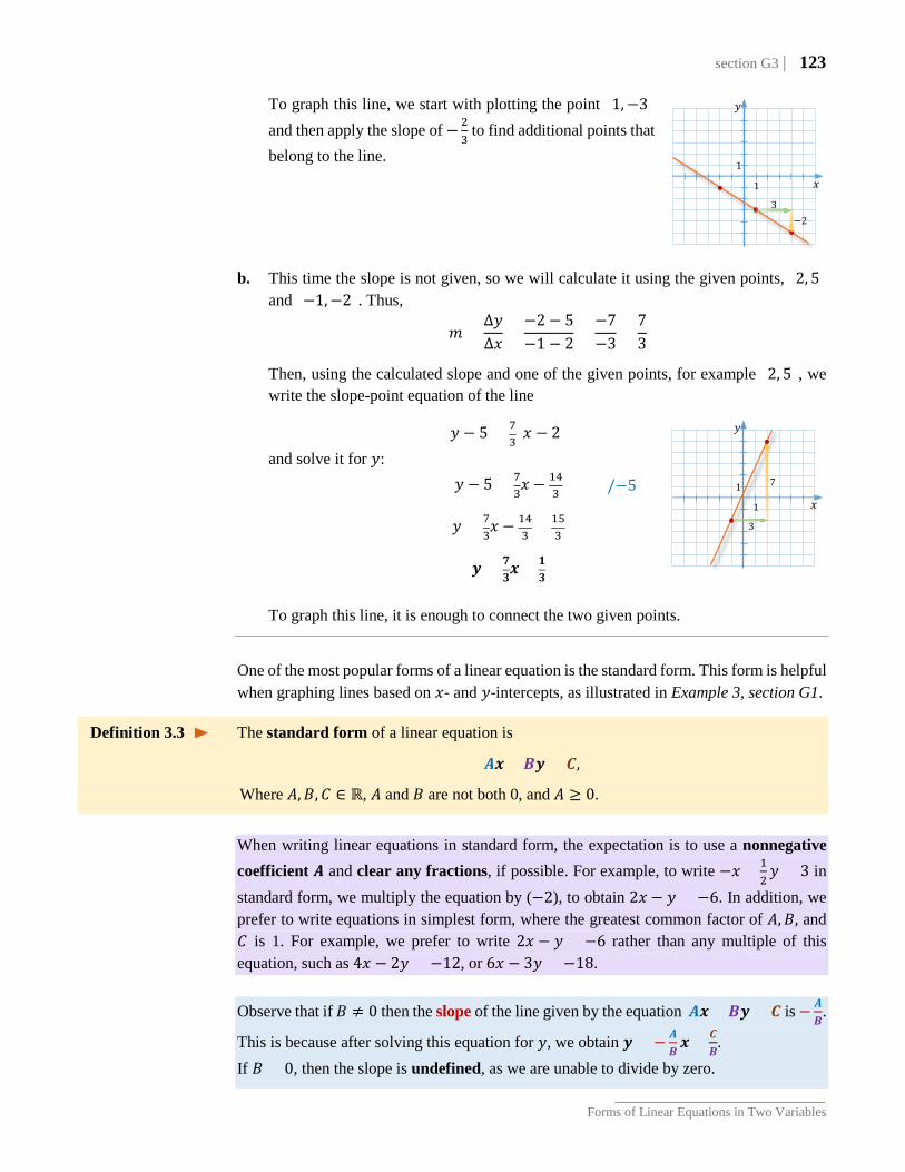
To graph this line, we start with plotting the point (1,−3) and then apply the slope of −2

3 to find additional points that

belong to the line.

b. This time the slope is not given, so we will calculate it using the given points, (2, 5)

and (−1,−2). Thus,

𝑚𝑚 =∆𝑦𝑦∆𝑥𝑥

=−2 − 5−1 − 2

=−7−3

=73

Then, using the calculated slope and one of the given points, for example (2, 5), we write the slope-point equation of the line

𝑦𝑦 − 5 = 73(𝑥𝑥 − 2)

and solve it for 𝑦𝑦: 𝑦𝑦 − 5 = 7

3𝑥𝑥 − 14

3

𝑦𝑦 = 73𝑥𝑥 − 14

3+ 15

3

𝒚𝒚 = 𝟕𝟕𝟑𝟑𝒙𝒙 + 𝟏𝟏

𝟑𝟑

To graph this line, it is enough to connect the two given points.

One of the most popular forms of a linear equation is the standard form. This form is helpful when graphing lines based on 𝑥𝑥- and 𝑦𝑦-intercepts, as illustrated in Example 3, section G1.

Definition 3.3 The standard form of a linear equation is

𝑨𝑨𝒙𝒙+ 𝑩𝑩𝒚𝒚 = 𝑪𝑪,

Where 𝐴𝐴,𝐵𝐵,𝐶𝐶 ∈ ℝ, 𝐴𝐴 and 𝐵𝐵 are not both 0, and 𝐴𝐴 ≥ 0.

When writing linear equations in standard form, the expectation is to use a nonnegative coefficient 𝑨𝑨 and clear any fractions, if possible. For example, to write −𝑥𝑥 + 1

2𝑦𝑦 = 3 in

standard form, we multiply the equation by (−2), to obtain 2𝑥𝑥 − 𝑦𝑦 = −6. In addition, we prefer to write equations in simplest form, where the greatest common factor of 𝐴𝐴,𝐵𝐵, and 𝐶𝐶 is 1. For example, we prefer to write 2𝑥𝑥 − 𝑦𝑦 = −6 rather than any multiple of this equation, such as 4𝑥𝑥 − 2𝑦𝑦 = −12, or 6𝑥𝑥 − 3𝑦𝑦 = −18. Observe that if 𝐵𝐵 ≠ 0 then the slope of the line given by the equation 𝑨𝑨𝒙𝒙 + 𝑩𝑩𝒚𝒚 = 𝑪𝑪 is −𝑨𝑨

𝑩𝑩.

This is because after solving this equation for 𝑦𝑦, we obtain 𝒚𝒚 = − 𝑨𝑨𝑩𝑩𝒙𝒙 + 𝑪𝑪

𝑩𝑩.

If 𝐵𝐵 = 0, then the slope is undefined, as we are unable to divide by zero.

𝑦𝑦

𝑥𝑥

7

1

3

1

𝑦𝑦

𝑥𝑥

−2

1

3

1

/−5

124 | section G3


The form of a linear equation that is most useful when writing equations of lines based on their 𝑥𝑥- and 𝑦𝑦-intercepts is the intercept form.

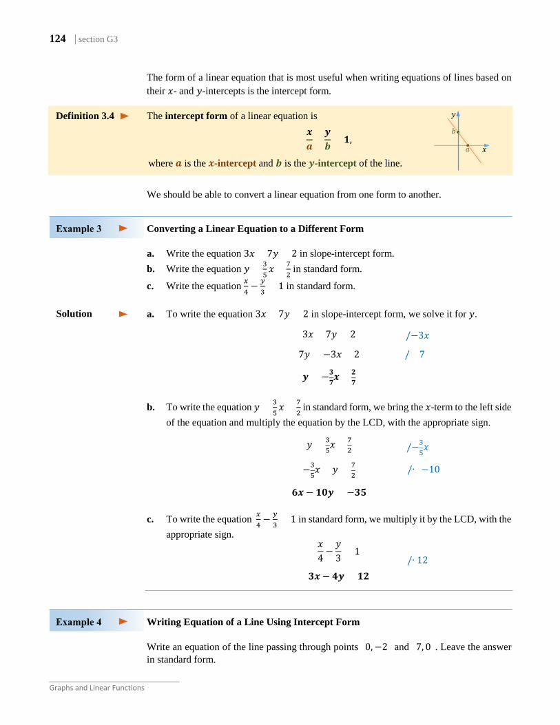
Definition 3.4 The intercept form of a linear equation is 𝒙𝒙𝒂𝒂

+𝒚𝒚𝒃𝒃

= 𝟏𝟏,

where 𝒂𝒂 is the 𝒙𝒙-intercept and 𝒃𝒃 is the 𝒚𝒚-intercept of the line.

We should be able to convert a linear equation from one form to another.

Converting a Linear Equation to a Different Form

a. Write the equation 3𝑥𝑥 + 7𝑦𝑦 = 2 in slope-intercept form. b. Write the equation 𝑦𝑦 = 3

5𝑥𝑥 + 7

2 in standard form.

c. Write the equation 𝑥𝑥4− 𝑦𝑦

3= 1 in standard form.

a. To write the equation 3𝑥𝑥 + 7𝑦𝑦 = 2 in slope-intercept form, we solve it for 𝑦𝑦.

3𝑥𝑥 + 7𝑦𝑦 = 2

7𝑦𝑦 = −3𝑥𝑥 + 2

𝒚𝒚 = −𝟑𝟑𝟕𝟕𝒙𝒙 + 𝟐𝟐

𝟕𝟕

b. To write the equation 𝑦𝑦 = 3

5𝑥𝑥 + 7

2 in standard form, we bring the 𝑥𝑥-term to the left side

of the equation and multiply the equation by the LCD, with the appropriate sign.

𝑦𝑦 = 35𝑥𝑥 + 7

2

−35𝑥𝑥 + 𝑦𝑦 = 7

2

𝟔𝟔𝒙𝒙 − 𝟏𝟏𝟎𝟎𝒚𝒚 = −𝟑𝟑𝟓𝟓 c. To write the equation 𝑥𝑥

4− 𝑦𝑦

3= 1 in standard form, we multiply it by the LCD, with the

appropriate sign. 𝑥𝑥4−𝑦𝑦3

= 1

𝟑𝟑𝒙𝒙 − 𝟒𝟒𝒚𝒚 = 𝟏𝟏𝟐𝟐

Writing Equation of a Line Using Intercept Form

Write an equation of the line passing through points (0,−2) and (7, 0). Leave the answer in standard form.

Solution

/−3𝑥𝑥

/÷ 7

/−35𝑥𝑥

/∙ (−10)

/∙ 12

𝑎𝑎

𝑦𝑦

𝑥𝑥

𝑏𝑏

section G3 | 125


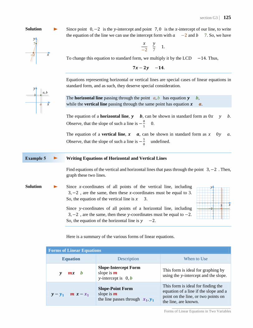
Since point (0,−2) is the 𝑦𝑦-intercept and point (7, 0) is the 𝑥𝑥-intercept of our line, to write the equation of the line we can use the intercept form with 𝑎𝑎 = −2 and 𝑏𝑏 = 7. So, we have

𝑥𝑥−2

+𝑦𝑦7

= 1.

To change this equation to standard form, we multiply it by the LCD = −14. Thus,

𝟕𝟕𝒙𝒙 − 𝟐𝟐𝒚𝒚 = −𝟏𝟏𝟒𝟒.

Equations representing horizontal or vertical lines are special cases of linear equations in standard form, and as such, they deserve special consideration. The horizontal line passing through the point (𝑎𝑎, 𝑏𝑏) has equation 𝒚𝒚 = 𝒃𝒃, while the vertical line passing through the same point has equation 𝒙𝒙 = 𝒂𝒂.

The equation of a horizontal line, 𝒚𝒚 = 𝒃𝒃, can be shown in standard form as 0𝑥𝑥 + 𝑦𝑦 = 𝑏𝑏. Observe, that the slope of such a line is −0

1= 0.

The equation of a vertical line, 𝒙𝒙 = 𝒂𝒂, can be shown in standard form as 𝑥𝑥 + 0𝑦𝑦 = 𝑎𝑎. Observe, that the slope of such a line is −1

0= undefined.

Writing Equations of Horizontal and Vertical Lines

Find equations of the vertical and horizontal lines that pass through the point (3,−2). Then, graph these two lines. Since 𝑥𝑥-coordinates of all points of the vertical line, including (3,−2), are the same, then these 𝑥𝑥-coordinates must be equal to 3. So, the equation of the vertical line is 𝑥𝑥 = 3.

Since 𝑦𝑦-coordinates of all points of a horizontal line, including (3,−2), are the same, then these 𝑦𝑦-coordinates must be equal to −2. So, the equation of the horizontal line is 𝑦𝑦 = −2.

Here is a summary of the various forms of linear equations.

Forms of Linear Equations

Equation Description When to Use

𝒚𝒚 = 𝒎𝒎𝒙𝒙 + 𝒃𝒃 Slope-Intercept Form slope is 𝒎𝒎 𝑦𝑦-intercept is (0,𝒃𝒃)

This form is ideal for graphing by using the 𝑦𝑦-intercept and the slope.

𝒚𝒚 − 𝒚𝒚𝟏𝟏 = 𝒎𝒎(𝒙𝒙 − 𝒙𝒙𝟏𝟏) Slope-Point Form slope is 𝒎𝒎 the line passes through (𝒙𝒙𝟏𝟏,𝒚𝒚𝟏𝟏)

This form is ideal for finding the equation of a line if the slope and a point on the line, or two points on the line, are known.

Solution

Solution 𝑦𝑦

𝑥𝑥 3 −2

−2

𝑦𝑦

𝑥𝑥

7

(𝑎𝑎,𝑏𝑏) 𝑦𝑦

𝑥𝑥

𝑏𝑏

𝑎𝑎

126 | section G3


Note: Except for the equations for a horizontal or vertical line, all of the above forms of

linear equations can be converted into each other via algebraic transformations.

Writing Equations of Parallel and Perpendicular Lines

Recall that the slopes of parallel lines are the same, and slopes of perpendicular lines are opposite reciprocals. See section G2.

Writing Equations of Parallel Lines Passing Through a Given Point

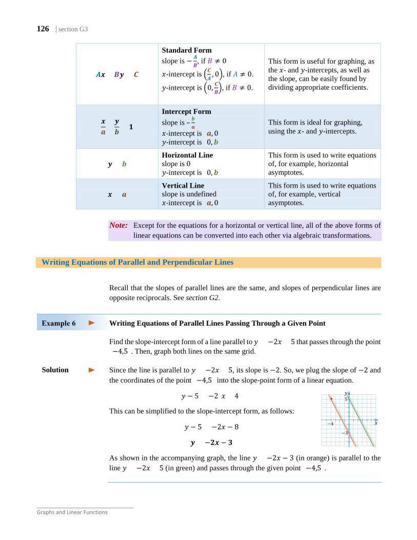
Find the slope-intercept form of a line parallel to 𝑦𝑦 = −2𝑥𝑥 + 5 that passes through the point (−4,5). Then, graph both lines on the same grid. Since the line is parallel to 𝑦𝑦 = −2𝑥𝑥 + 5, its slope is −2. So, we plug the slope of −2 and the coordinates of the point (−4,5) into the slope-point form of a linear equation.

𝑦𝑦 − 5 = −2(𝑥𝑥 + 4)

This can be simplified to the slope-intercept form, as follows:

𝑦𝑦 − 5 = −2𝑥𝑥 − 8

𝒚𝒚 = −𝟐𝟐𝒙𝒙 − 𝟑𝟑

As shown in the accompanying graph, the line 𝑦𝑦 = −2𝑥𝑥 − 3 (in orange) is parallel to the line 𝑦𝑦 = −2𝑥𝑥 + 5 (in green) and passes through the given point (−4,5).

𝑨𝑨𝒙𝒙 +𝑩𝑩𝒚𝒚 = 𝑪𝑪

Standard Form slope is − 𝑨𝑨

𝑩𝑩, if 𝐵𝐵 ≠ 0

𝑥𝑥-intercept is �𝑪𝑪𝑨𝑨

, 0�, if 𝐴𝐴 ≠ 0.

𝑦𝑦-intercept is �0, 𝑪𝑪𝑩𝑩�, if 𝐵𝐵 ≠ 0.

This form is useful for graphing, as the 𝑥𝑥- and 𝑦𝑦-intercepts, as well as the slope, can be easily found by dividing appropriate coefficients.

𝒙𝒙𝒂𝒂

+𝒚𝒚𝒃𝒃

= 𝟏𝟏

Intercept Form slope is – 𝒃𝒃

𝒂𝒂

𝑥𝑥-intercept is (𝒂𝒂, 0) 𝑦𝑦-intercept is (0,𝒃𝒃)

This form is ideal for graphing, using the 𝑥𝑥- and 𝑦𝑦-intercepts.

𝒚𝒚 = 𝒃𝒃 Horizontal Line slope is 0 𝑦𝑦-intercept is (0,𝒃𝒃)

This form is used to write equations of, for example, horizontal asymptotes.

𝒙𝒙 = 𝒂𝒂 Vertical Line slope is undefined 𝑥𝑥-intercept is (𝒂𝒂, 0)

This form is used to write equations of, for example, vertical asymptotes.

Solution

𝑦𝑦

𝑥𝑥

5

−4

−3

section G3 | 127


Writing Equations of Perpendicular Lines Passing Through a Given Point

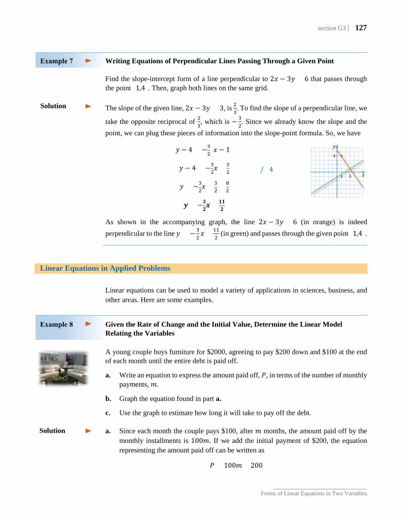
Find the slope-intercept form of a line perpendicular to 2𝑥𝑥 − 3𝑦𝑦 = 6 that passes through the point (1,4). Then, graph both lines on the same grid. The slope of the given line, 2𝑥𝑥 − 3𝑦𝑦 = 3, is 2

3. To find the slope of a perpendicular line, we

take the opposite reciprocal of 23, which is −3

2. Since we already know the slope and the

point, we can plug these pieces of information into the slope-point formula. So, we have

𝑦𝑦 − 4 = −32(𝑥𝑥 − 1)

𝑦𝑦 − 4 = −32𝑥𝑥 + 3

2

𝑦𝑦 = −32𝑥𝑥 + 3

2+ 8

2

𝒚𝒚 = −𝟑𝟑𝟐𝟐𝒙𝒙 + 𝟏𝟏𝟏𝟏

𝟐𝟐

As shown in the accompanying graph, the line 2𝑥𝑥 − 3𝑦𝑦 = 6 (in orange) is indeed perpendicular to the line 𝑦𝑦 = −3

2𝑥𝑥 + 11

2 (in green) and passes through the given point (1,4).

Linear Equations in Applied Problems

Linear equations can be used to model a variety of applications in sciences, business, and other areas. Here are some examples.

Given the Rate of Change and the Initial Value, Determine the Linear Model Relating the Variables

A young couple buys furniture for $2000, agreeing to pay $200 down and $100 at the end of each month until the entire debt is paid off.

a. Write an equation to express the amount paid off, 𝑃𝑃, in terms of the number of monthly payments, 𝑚𝑚.

b. Graph the equation found in part a.

c. Use the graph to estimate how long it will take to pay off the debt. a. Since each month the couple pays $100, after 𝑚𝑚 months, the amount paid off by the

monthly installments is 100𝑚𝑚. If we add the initial payment of $200, the equation representing the amount paid off can be written as

𝑃𝑃 = 100𝑚𝑚 + 200

Solution

𝑦𝑦

𝑥𝑥

4

3 1 /+4

Solution

128 | section G3


b. To graph this equation, we use the slope-intercept method. Starting with the 𝑃𝑃-intercept of 200, we run 1 and rise 100, repeating this process as many times as needed to hit a lattice point on the chosen scale. So, as shown in the accompanying graph, the line passes through points (6, 800) and (18, 2000).

c. As shown in the graph, $2000 will be paid off in 18 months.

Finding a Linear Equation that Fits the Data Given by Two Ordered Pairs

Gabriel Daniel Fahrenheit invented the mercury thermometer in 1717. The thermometer shows that water freezes at 32℉ and boils at 212℉. In 1742, Anders Celsius invented the Celsius temperature scale. On this scale, water freezes at 0℃ and boils at 100℃. Determine a linear equation that can be used to predict the Celsius temperature, 𝐶𝐶, when the Fahrenheit temperature, 𝐹𝐹, is known. To predict the Celsius temperature, 𝐶𝐶, knowing the Fahrenheit temperature, 𝐹𝐹, we treat the variable 𝐶𝐶 as dependent on the variable 𝐹𝐹. So, we consider 𝐶𝐶 as the second coordinate when setting up the ordered pairs, (𝐹𝐹,𝐶𝐶), of given data. The corresponding freezing temperatures give us the pair (32,0) and the boiling temperatures give us the pair (212,100). To find the equation of a line passing through these two points, first, we calculate the slope, and then, we use the slope-point formula. So, the slope is

𝑚𝑚 =100 − 0

212− 32=

100180

=𝟓𝟓𝟗𝟗

,

and using the point (32,0), the equation of the line is

𝑪𝑪 =𝟓𝟓𝟗𝟗

(𝑭𝑭 − 𝟑𝟑𝟐𝟐)

Determining if the Given Set of Data Follows a Linear Pattern

Determine whether the data given in each table follow a linear pattern. If they do, find the slope-intercept form of an equation of the line passing through all the given points.

a.

a. The set of points follows a linear pattern if the slopes between consecutive pairs of these points are the same. These slopes are the ratios of increments in 𝑦𝑦-values to increments in 𝑥𝑥-values. Notice that the increases between successive 𝑥𝑥-values of the given points are constantly equal to 2. So, to check if the points follow a linear pattern, it is enough to check if the increases between successive 𝑦𝑦-values are also constant. Observe that the numbers in the list 12, 16, 20, 24, 28 steadily increase by 4. Thus, the given set of data follow a linear pattern.

x 1 3 5 7 9 y 12 16 20 24 28

x 10 20 30 40 50 y 15 21 26 30 35

3 9 18

1600

1200

𝑃𝑃

𝑚𝑚

400

6

2000

12

(6,800)

(18,2000)

800

15

Solution

Solution

b.

section G3 | 129


To find an equation of the line passing through these points, we use the slope, which is 42

= 2, and one of the given points, for example (1,12). By plugging these pieces of information into the slope-point formula, we obtain

𝑦𝑦 − 12 = 2(𝑥𝑥 − 1), which after simplifying becomes

𝑦𝑦 − 12 = 2𝑥𝑥 − 2

𝒚𝒚 = 𝟐𝟐𝒙𝒙 + 𝟏𝟏𝟎𝟎

b. Observe that the increments between consecutive 𝑥𝑥-values of the given points are constantly equal to 10, while the increments between consecutive 𝑦𝑦-values in the list 15, 21, 26, 30, 35 are 6, 5, 4, 5. So, they are not constant. Therefore, the given set of data does not follow a linear pattern.

Finding a Linear Model Relating the Number of Items Bought at a Fixed Amount

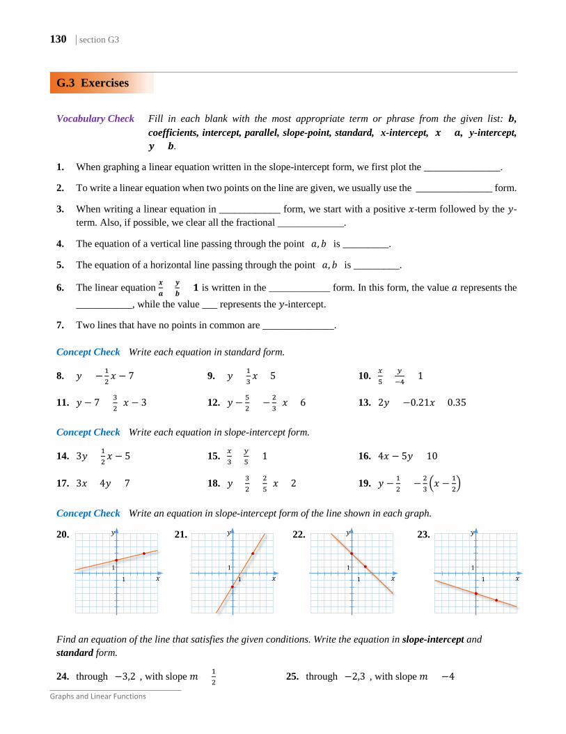
A manager for a country market buys apples at $0.25 each and pears at $0.50 each. Write a linear equation in standard form relating the number of apples, 𝑎𝑎, and pears, 𝑝𝑝, she can buy for $80. Then, a. graph the equation and b. using the graph, find at least 3 points (𝑎𝑎,𝑝𝑝) satisfying the equation, and interpret their

meanings in the context of the problem. It costs 0.25𝑎𝑎 dollars to buy 𝑎𝑎 apples. Similarly, it costs 0.50𝑝𝑝 dollars to buy 𝑝𝑝 pears. Since the total charge is $80, we have

0.25𝑎𝑎 + 0.50𝑝𝑝 = 80

We could convert the coefficients into integers by multiplying the equation by a hundred. So, we obtain

25𝑎𝑎 + 50𝑝𝑝 = 8000, which, after dividing by 25, turns into

𝒂𝒂 + 𝟐𝟐𝒔𝒔 = 𝟑𝟑𝟐𝟐𝟎𝟎.

a. To graph this equation, we will represent the number of apples, 𝑎𝑎, on the horizontal axis and the number of pears, 𝑝𝑝, on the vertical axis, respecting the alphabetical order of labelling the axes. Using the intercept method, we connect points (320,0) and (0,160).

b. Aside of the intercepts, (320,0) and (0,160), the graph shows us a few more points that satisfy the equation. In particular, (𝟖𝟖𝟎𝟎,𝟏𝟏𝟐𝟐𝟎𝟎) and (𝟏𝟏𝟔𝟔𝟎𝟎,𝟖𝟖𝟎𝟎) are points of the graph. If a point (𝑎𝑎,𝑝𝑝) of the graph has integral coefficients, it tells us that for $80, the manager could buy a apples and p pears. For example, the point (𝟖𝟖𝟎𝟎,𝟏𝟏𝟐𝟐𝟎𝟎) tells us that the manager can buy 80 apples and 120 pears for $80.

Solution

𝑝𝑝

𝑎𝑎

80

160

160

320

(80,120) (160,80)

(320,0)

/+12

130 | section G3


G.3 Exercises

Vocabulary Check Fill in each blank with the most appropriate term or phrase from the given list: 𝒃𝒃,

coefficients, intercept, parallel, slope-point, standard, x-intercept, 𝒙𝒙 = 𝒂𝒂, y-intercept, 𝒚𝒚 = 𝒃𝒃.

1. When graphing a linear equation written in the slope-intercept form, we first plot the _______________.

2. To write a linear equation when two points on the line are given, we usually use the _______________ form.

3. When writing a linear equation in ____________ form, we start with a positive 𝑥𝑥-term followed by the 𝑦𝑦-term. Also, if possible, we clear all the fractional _____________.

4. The equation of a vertical line passing through the point (𝑎𝑎, 𝑏𝑏) is _________.

5. The equation of a horizontal line passing through the point (𝑎𝑎, 𝑏𝑏) is _________.

6. The linear equation 𝒙𝒙𝒂𝒂

+ 𝒚𝒚𝒃𝒃

= 𝟏𝟏 is written in the ____________ form. In this form, the value 𝑎𝑎 represents the ___________, while the value ___ represents the 𝑦𝑦-intercept.

7. Two lines that have no points in common are ______________. Concept Check Write each equation in standard form.

8. 𝑦𝑦 = −12𝑥𝑥 − 7 9. 𝑦𝑦 = 1

3𝑥𝑥 + 5 10. 𝑥𝑥

5+ 𝑦𝑦

−4= 1

11. 𝑦𝑦 − 7 = 32

(𝑥𝑥 − 3) 12. 𝑦𝑦 − 52

= −23

(𝑥𝑥 + 6) 13. 2𝑦𝑦 = −0.21𝑥𝑥 + 0.35 Concept Check Write each equation in slope-intercept form.

14. 3𝑦𝑦 = 12𝑥𝑥 − 5 15. 𝑥𝑥

3+ 𝑦𝑦

5= 1 16. 4𝑥𝑥 − 5𝑦𝑦 = 10

17. 3𝑥𝑥 + 4𝑦𝑦 = 7 18. 𝑦𝑦 + 32

= 25

(𝑥𝑥 + 2) 19. 𝑦𝑦 − 12

= −23�𝑥𝑥 − 1

2�

Concept Check Write an equation in slope-intercept form of the line shown in each graph.

20. 21. 22. 23.

Find an equation of the line that satisfies the given conditions. Write the equation in slope-intercept and standard form.

24. through (−3,2), with slope 𝑚𝑚 = 12 25. through (−2,3), with slope 𝑚𝑚 = −4

𝑦𝑦

𝑥𝑥 1

1

𝑦𝑦

𝑥𝑥 1

1

𝑦𝑦

𝑥𝑥 1

1

𝑦𝑦

𝑥𝑥 1

1

section G3 | 131


26. with slope 𝑚𝑚 = 32 and 𝑦𝑦-intercept at −1 27. with slope 𝑚𝑚 = −1

5 and 𝑦𝑦-intercept at 2

28. through (−1,−2), with 𝑦𝑦-intercept at −3 29. through (−4,5), with 𝑦𝑦-intercept at 32

30. through (2,−1) and (−4,6) 31. through (3,7) and (−5,1)

32. through �− 43

,−2� and �45

, 23� 33. through �4

3, 32� and �− 1

2, 43�

Find an equation of the line that satisfies the given conditions.

34. through (−5,7), with slope 0 35. through (−2,−4), with slope 0

36. through (−1,−2), with undefined slope 37. through (−3,4), with undefined slope

38. through (−3,6) and horizontal 39. through �− 53

,−72� and horizontal

40. through �− 34

,−32� and vertical 41. through (5,−11) and vertical

Concept Check Write an equation in standard form for each of the lines described. In each case make a sketch

of the given line and the line satisfying the conditions.

42. through (7,2) and parallel to 3𝑥𝑥 − 𝑦𝑦 = 4 43. through (4,1) and parallel to 2𝑥𝑥 + 5𝑦𝑦 = 10

44. through (−2,3) and parallel to −𝑥𝑥 + 2𝑦𝑦 = 6 45. through (−1,−3) and parallel to −𝑥𝑥 + 3𝑦𝑦 = 12

46. through (−1,2) and parallel to 𝑦𝑦 = 3 47. through (−1,2) and parallel to 𝑥𝑥 = −3

48. through (6,2) and perpendicular to 2𝑥𝑥 − 𝑦𝑦 = 5 49. through (0,2) and perpendicular to 5𝑥𝑥 + 𝑦𝑦 = 15

50. through (−2,4) and perpendicular to 3𝑥𝑥 + 𝑦𝑦 = 6 51. through (−4,−1) and perpendicular to 𝑥𝑥 − 3𝑦𝑦 = 9

52. through (3,−4) and perpendicular to 𝑥𝑥 = 2 53. through (3,−4) and perpendicular to 𝑦𝑦 = −3

Analytic Skills For each situation, write an equation in the form y = mx + b, and then answer the question of the problem.

54. Membership in the Midwest Athletic Club costs $99, plus $41 per month. Let 𝑥𝑥 represent the number of months and 𝑦𝑦 represent the cost. How much does one-year membership cost?

55. A cell phone plan includes 900 anytime minutes for $60 per month, plus a one-time activation fee of $36. A cell phone is included at no additional charge. Let 𝑥𝑥 represent the number of months of service and 𝑦𝑦 represent the cost. If you sign a 1-yr contract, how much will this cell phone plan cost?

56. There is a $30 fee to rent a chainsaw, plus $6 per day. Let 𝑥𝑥 represent the number of days the saw is rented and 𝑦𝑦 represent the total charge to the renter, in dollars. If the total charge is $138, for how many days is the saw rented?

57. A rental car costs $50 plus $0.12 per kilometer. Let 𝑥𝑥 represent the number of kilometers driven and 𝑦𝑦 represent the total charge to the renter, in dollars. How many kilometers was the car driven if the renter paid $84.20?

132 | section G3


Analytic Skills Solve each problem.

58. At its inception, a professional organization had 26 members. Three years later, the organization had grown to 83 members. If membership continues to grow at the same rate, find an equation that represents the number 𝑟𝑟 of members in the organization after 𝑚𝑚 years.

59. Thirty minutes after a truck driver passes the 142-km marker on a freeway, he passes the 170-km marker. Find an equation that shows the distance 𝑑𝑑 he drives in 𝑚𝑚 hr.

60. The average annual cost of a private college or university is shown in the table. This cost includes tuition, fees, room, and board.

a. Find the slope-intercept form of a line that passes through these two data points. b. Interpret the slope in the context of the problem. c. To the nearest thousand, estimate the cost of private college or university in 2020.

61. The life expectancy for a person born in 1900 was 48 years, and in 2000 it was 77 years. To the nearest year, estimate the life expectancy for someone born in 1970.

62. After 2 years, the amount in a savings account earning simple interest was $1070. After 5 years, the amount in the account was $1175. Find an equation that represents the amount 𝐴𝐴 in the account after 𝑚𝑚 years.

63. A real-estate agent receives a flat monthly salary plus a 0.5% commission on her monthly home sales. In a particular month, her home sales were $500,000, and her total monthly income was $4300.

a. Write an equation in slope-intercept form that shows the real-estate agent’s total monthly income 𝐼𝐼 in terms of her monthly home sales 𝑟𝑟.

b. Graph the equation on the coordinate plane. c. What does the 𝐼𝐼-intercept represent in the context of the problem? d. What does the slope represent in the context of the problem?

64. A taxi company charges a flat meter fare of $1.25 plus an additional fee for each kilometer (or part thereof) driven. A passenger pays $10.25 for a 6-kilometer taxi ride.

a. Find an equation in slope-intercept form that models the total meter fare 𝑓𝑓 in terms of the number 𝑘𝑘 of kilometers driven.

b. Graph the equation on the coordinate plane. c. What does the slope of the graph of the equation in part a. represent in this situation? d. How many kilometers were driven if a passenger pays $20.75?

65. Fold a string like this:

Count how many pieces of string you would have after cutting the string as shown in Figure 3.1. Predict how many pieces of string you would have if you made 2, 3, or more such cuts. Complete the table below and determine whether or not the data in the table follow a linear pattern. Can you find an equation that predicts the number of pieces if you know the number of cuts?

Year 𝒚𝒚 2007 2016 Cost 𝑪𝑪 $37000 $72000

# of cuts 0 1 2 3 4 5 # of pieces

cutline

Figure 3.1

section G4 | 133

Linear Inequalities in Two Variables Including Systems of Inequalities

G.4 Linear Inequalities in Two Variables Including Systems of Inequalities

In many real-life situations, we are interested in a range of values satisfying certain conditions rather than in one specific value. For example, when exercising, we like to keep the heart rate between 120 and 140 beats per minute. The systolic blood pressure of a healthy person is usually between 100 and 120 mmHg (millimeters of mercury). Such conditions can be described using inequalities. Solving systems of inequalities has its applications in many practical business problems, such as how to allocate resources to achieve a maximum profit or a minimum cost. In this section, we study graphical solutions of linear inequalities and systems of linear inequalities.

Linear Inequalities in Two Variables

Definition 4.1 Any inequality that can be written as

𝑨𝑨𝑨𝑨 + 𝑩𝑩𝑩𝑩 < 𝑪𝑪, 𝑨𝑨𝑨𝑨 + 𝑩𝑩𝑩𝑩 ≤ 𝑪𝑪, 𝑨𝑨𝑨𝑨+ 𝑩𝑩𝑩𝑩 > 𝑪𝑪, 𝑨𝑨𝑨𝑨 + 𝑩𝑩𝑩𝑩 ≥ 𝑪𝑪, or 𝑨𝑨𝑨𝑨 + 𝑩𝑩𝑩𝑩 ≠ 𝑪𝑪,

where 𝐴𝐴,𝐵𝐵,𝐶𝐶 ∈ ℝ and 𝐴𝐴 and 𝐵𝐵 are not both 0, is a linear inequality in two variables.

To solve an inequality in two variables, 𝑥𝑥 and 𝑦𝑦, means to find all ordered pairs (𝑨𝑨,𝑩𝑩) satisfying the inequality.

Inequalities in two variables arise from many situations. For example, suppose that the number of full-time students, 𝑓𝑓, and part-time students, 𝑝𝑝, enrolled in upgrading courses at the University of the Fraser Valley is at most 1200. This situation can be represented by the inequality

𝑓𝑓 + 𝑝𝑝 ≤ 1200.

Some of the solutions (𝑓𝑓,𝑝𝑝) of this inequality are: (1000, 200), (1000, 199), (1000, 198), (600, 600). (550, 600), (1100, 0), and many others.

The solution sets of inequalities in two variables contain infinitely many ordered pairs of numbers which, when graphed in a system of coordinates, fulfill specific regions of the coordinate plane. That is why it is more beneficial to present such solutions in the form of a graph rather than using set notation. To graph the region of points satisfying the inequality 𝑓𝑓 + 𝑝𝑝 ≤ 1200, we may want to solve it first for 𝑝𝑝,

𝑝𝑝 ≤ −𝑓𝑓 + 1200,

and then graph the related equation, 𝑝𝑝 = −𝑓𝑓 + 1200, called the boundary line. Notice, that setting 𝑓𝑓 to, for instance, 300 results in the inequality

𝑝𝑝 ≤ −300 + 1200 = 900. So, any point with the first coordinate of 300 and the second coordinate of 900 or less satisfies the inequality (see the dotted half-line in Figure 1a). Generally, observe that any point with the first coordinate 𝑓𝑓 and the second coordinate −𝑓𝑓 +1200 or less satisfies the inequality. Since the union of all half-lines that start from the boundary line and go down is the whole half-plane below the boundary line, Figure 1a

𝑝𝑝

𝑓𝑓

300

1200

1200

300

(300,900)

134 | section G4


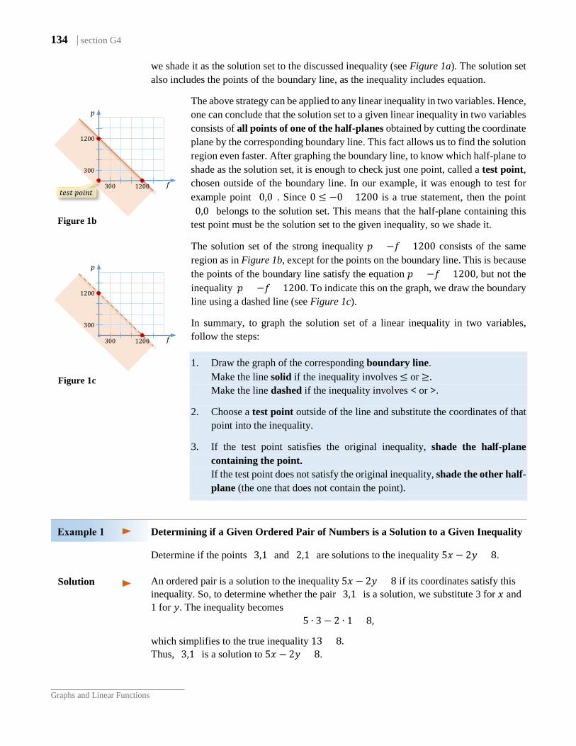
we shade it as the solution set to the discussed inequality (see Figure 1a). The solution set also includes the points of the boundary line, as the inequality includes equation.

The above strategy can be applied to any linear inequality in two variables. Hence, one can conclude that the solution set to a given linear inequality in two variables consists of all points of one of the half-planes obtained by cutting the coordinate plane by the corresponding boundary line. This fact allows us to find the solution region even faster. After graphing the boundary line, to know which half-plane to shade as the solution set, it is enough to check just one point, called a test point, chosen outside of the boundary line. In our example, it was enough to test for example point (0,0). Since 0 ≤ −0 + 1200 is a true statement, then the point (0,0) belongs to the solution set. This means that the half-plane containing this test point must be the solution set to the given inequality, so we shade it.

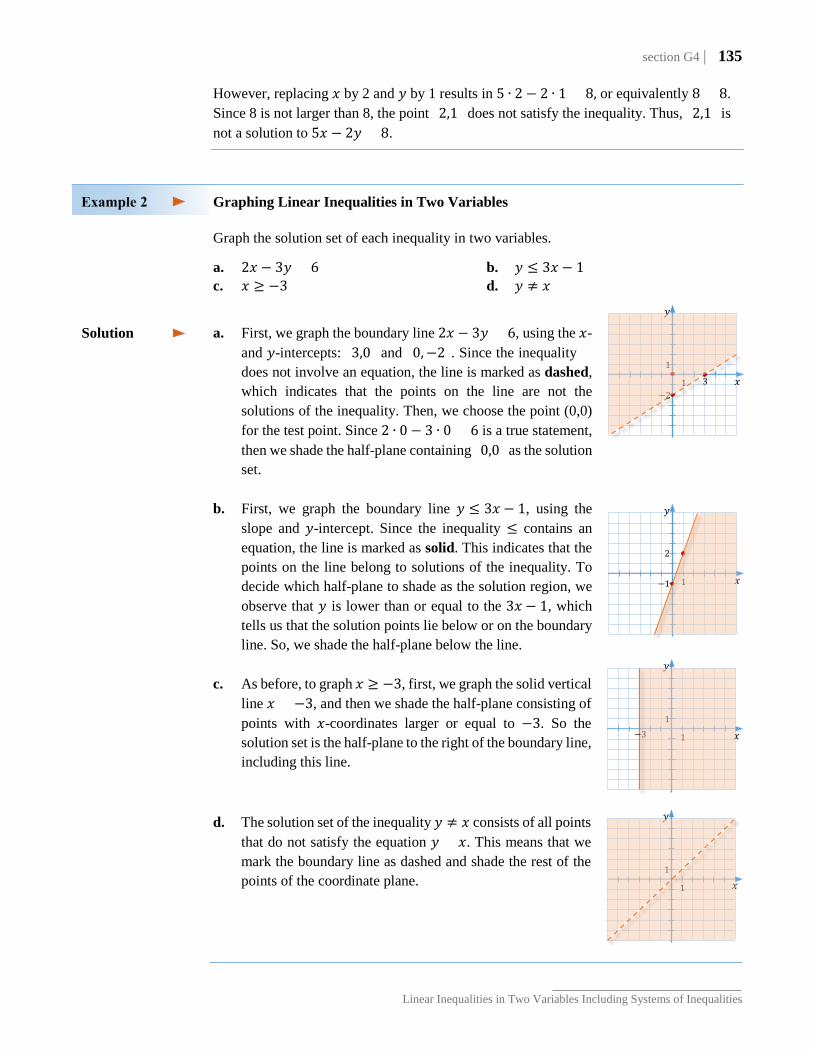
The solution set of the strong inequality 𝑝𝑝 < −𝑓𝑓 + 1200 consists of the same region as in Figure 1b, except for the points on the boundary line. This is because the points of the boundary line satisfy the equation 𝑝𝑝 = −𝑓𝑓 + 1200, but not the inequality 𝑝𝑝 < −𝑓𝑓 + 1200. To indicate this on the graph, we draw the boundary line using a dashed line (see Figure 1c).

In summary, to graph the solution set of a linear inequality in two variables, follow the steps:

1. Draw the graph of the corresponding boundary line. Make the line solid if the inequality involves ≤ or ≥. Make the line dashed if the inequality involves < or >.

2. Choose a test point outside of the line and substitute the coordinates of that point into the inequality.

3. If the test point satisfies the original inequality, shade the half-plane containing the point.

If the test point does not satisfy the original inequality, shade the other half-plane (the one that does not contain the point).

Determining if a Given Ordered Pair of Numbers is a Solution to a Given Inequality Determine if the points (3,1) and (2,1) are solutions to the inequality 5𝑥𝑥 − 2𝑦𝑦 > 8.

An ordered pair is a solution to the inequality 5𝑥𝑥 − 2𝑦𝑦 > 8 if its coordinates satisfy this inequality. So, to determine whether the pair (3,1) is a solution, we substitute 3 for 𝑥𝑥 and 1 for 𝑦𝑦. The inequality becomes

5 ∙ 3 − 2 ∙ 1 > 8,

which simplifies to the true inequality 13 > 8. Thus, (3,1) is a solution to 5𝑥𝑥 − 2𝑦𝑦 > 8.

Figure 1c

Figure 1b

𝑝𝑝

𝑓𝑓

300

1200

1200

300 𝑡𝑡𝑡𝑡𝑡𝑡𝑡𝑡 𝑝𝑝𝑝𝑝𝑝𝑝𝑝𝑝𝑡𝑡

𝑝𝑝

𝑓𝑓

300

1200

1200

300

Solution

section G4 | 135


However, replacing 𝑥𝑥 by 2 and 𝑦𝑦 by 1 results in 5 ∙ 2 − 2 ∙ 1 > 8, or equivalently 8 > 8. Since 8 is not larger than 8, the point (2,1) does not satisfy the inequality. Thus, (2,1) is not a solution to 5𝑥𝑥 − 2𝑦𝑦 > 8.

Graphing Linear Inequalities in Two Variables Graph the solution set of each inequality in two variables.

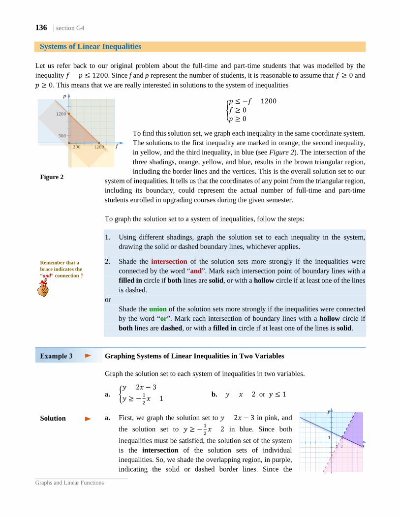
a. 2𝑥𝑥 − 3𝑦𝑦 < 6 b. 𝑦𝑦 ≤ 3𝑥𝑥 − 1 c. 𝑥𝑥 ≥ −3 d. 𝑦𝑦 ≠ 𝑥𝑥

a. First, we graph the boundary line 2𝑥𝑥 − 3𝑦𝑦 = 6, using the 𝑥𝑥- and 𝑦𝑦-intercepts: (3,0) and (0,−2). Since the inequality < does not involve an equation, the line is marked as dashed, which indicates that the points on the line are not the solutions of the inequality. Then, we choose the point (0,0) for the test point. Since 2 ∙ 0 − 3 ∙ 0 < 6 is a true statement, then we shade the half-plane containing (0,0) as the solution set.

b. First, we graph the boundary line 𝑦𝑦 ≤ 3𝑥𝑥 − 1, using the

slope and 𝑦𝑦-intercept. Since the inequality ≤ contains an equation, the line is marked as solid. This indicates that the points on the line belong to solutions of the inequality. To decide which half-plane to shade as the solution region, we observe that 𝑦𝑦 is lower than or equal to the 3𝑥𝑥 − 1, which tells us that the solution points lie below or on the boundary line. So, we shade the half-plane below the line.

c. As before, to graph 𝑥𝑥 ≥ −3, first, we graph the solid vertical

line 𝑥𝑥 = −3, and then we shade the half-plane consisting of points with 𝑥𝑥-coordinates larger or equal to −3. So the solution set is the half-plane to the right of the boundary line, including this line.

d. The solution set of the inequality 𝑦𝑦 ≠ 𝑥𝑥 consists of all points that do not satisfy the equation 𝑦𝑦 = 𝑥𝑥. This means that we mark the boundary line as dashed and shade the rest of the points of the coordinate plane.

Solution 𝑦𝑦

𝑥𝑥 3 1 −2

1

𝑦𝑦

𝑥𝑥 −3 1

1

𝑦𝑦

𝑥𝑥

2

1 −1

𝑦𝑦

𝑥𝑥 1

1

136 | section G4


Systems of Linear Inequalities Let us refer back to our original problem about the full-time and part-time students that was modelled by the inequality 𝑓𝑓 + 𝑝𝑝 ≤ 1200. Since f and p represent the number of students, it is reasonable to assume that 𝑓𝑓 ≥ 0 and 𝑝𝑝 ≥ 0. This means that we are really interested in solutions to the system of inequalities

�𝑝𝑝 ≤ −𝑓𝑓 + 1200𝑓𝑓 ≥ 0 𝑝𝑝 ≥ 0

To find this solution set, we graph each inequality in the same coordinate system. The solutions to the first inequality are marked in orange, the second inequality, in yellow, and the third inequality, in blue (see Figure 2). The intersection of the three shadings, orange, yellow, and blue, results in the brown triangular region, including the border lines and the vertices. This is the overall solution set to our

system of inequalities. It tells us that the coordinates of any point from the triangular region, including its boundary, could represent the actual number of full-time and part-time students enrolled in upgrading courses during the given semester. To graph the solution set to a system of inequalities, follow the steps:

1. Using different shadings, graph the solution set to each inequality in the system, drawing the solid or dashed boundary lines, whichever applies.

2. Shade the intersection of the solution sets more strongly if the inequalities were connected by the word “and”. Mark each intersection point of boundary lines with a filled in circle if both lines are solid, or with a hollow circle if at least one of the lines is dashed.

or Shade the union of the solution sets more strongly if the inequalities were connected

by the word “or”. Mark each intersection of boundary lines with a hollow circle if both lines are dashed, or with a filled in circle if at least one of the lines is solid.

Graphing Systems of Linear Inequalities in Two Variables Graph the solution set to each system of inequalities in two variables.

a. �𝑦𝑦 < 2𝑥𝑥 − 3𝑦𝑦 ≥ −1

2𝑥𝑥 + 1 b. 𝑦𝑦 > 𝑥𝑥 + 2 or 𝑦𝑦 ≤ 1

a. First, we graph the solution set to 𝑦𝑦 < 2𝑥𝑥 − 3 in pink, and

the solution set to 𝑦𝑦 ≥ −12𝑥𝑥 + 2 in blue. Since both

inequalities must be satisfied, the solution set of the system is the intersection of the solution sets of individual inequalities. So, we shade the overlapping region, in purple, indicating the solid or dashed border lines. Since the

Figure 2

Solution

𝑝𝑝

𝑓𝑓

300

1200

1200

300

𝑦𝑦

𝑥𝑥 1 2

1

Remember that a brace indicates the “and” connection

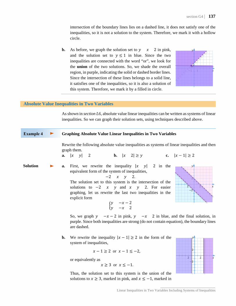
section G4 | 137


intersection of the boundary lines lies on a dashed line, it does not satisfy one of the inequalities, so it is not a solution to the system. Therefore, we mark it with a hollow circle.

b. As before, we graph the solution set to 𝑦𝑦 > 𝑥𝑥 + 2 in pink,

and the solution set to 𝑦𝑦 ≤ 1 in blue. Since the two inequalities are connected with the word “or”, we look for the union of the two solutions. So, we shade the overall region, in purple, indicating the solid or dashed border lines. Since the intersection of these lines belongs to a solid line, it satisfies one of the inequalities, so it is also a solution of this system. Therefore, we mark it by a filled in circle.

Absolute Value Inequalities in Two Variables

As shown in section L6, absolute value linear inequalities can be written as systems of linear inequalities. So we can graph their solution sets, using techniques described above.

Graphing Absolute Value Linear Inequalities in Two Variables

Rewrite the following absolute value inequalities as systems of linear inequalities and then graph them. a. |𝑥𝑥 + 𝑦𝑦| < 2 b. |𝑥𝑥 + 2| ≥ 𝑦𝑦 c. |𝑥𝑥 − 1| ≥ 2 a. First, we rewrite the inequality |𝑥𝑥 + 𝑦𝑦| < 2 in the

equivalent form of the system of inequalities, −2 < 𝑥𝑥 + 𝑦𝑦 < 2.

The solution set to this system is the intersection of the solutions to −2 < 𝑥𝑥 + 𝑦𝑦 and 𝑥𝑥 + 𝑦𝑦 < 2. For easier graphing, let us rewrite the last two inequalities in the explicit form

�𝑦𝑦 > −𝑥𝑥 − 2𝑦𝑦 < −𝑥𝑥 + 2

So, we graph 𝑦𝑦 > −𝑥𝑥 − 2 in pink, 𝑦𝑦 < −𝑥𝑥 + 2 in blue, and the final solution, in purple. Since both inequalities are strong (do not contain equation), the boundary lines are dashed.

b. We rewrite the inequality |𝑥𝑥 − 1| ≥ 2 in the form of the

system of inequalities,

𝑥𝑥 − 1 ≥ 2 or 𝑥𝑥 − 1 ≤ −2,

or equivalently as 𝑥𝑥 ≥ 3 or 𝑥𝑥 ≤ −1.

Thus, the solution set to this system is the union of the solutions to 𝑥𝑥 ≥ 3, marked in pink, and 𝑥𝑥 ≤ −1, marked in

𝑦𝑦

𝑥𝑥 1 −1

1

Solution 𝑦𝑦

𝑥𝑥 −2

2

2

2

𝑦𝑦

𝑥𝑥 −2

2

2

2

138 | section G4


blue. The overall solution to the system is marked in purple and includes the boundary lines.

c. We rewrite the inequality |𝑥𝑥 + 2| ≤ 𝑦𝑦 in the form of the

system of inequalities,

−𝑦𝑦 ≤ 𝑥𝑥 + 2 ≤ 𝑦𝑦,

or equivalently as 𝑦𝑦 ≥ −𝑥𝑥 − 2 and 𝑦𝑦 ≥ 𝑥𝑥 + 2.

Thus, the solution set to this system is the intersection of the solutions to 𝑦𝑦 ≥ −𝑥𝑥 − 2, marked in pink, and 𝑦𝑦 ≥ 𝑥𝑥 + 2, marked in blue. The overall solution to the system, marked in purple, includes the border lines and the vertex.

G.4 Exercises

Vocabulary Check Fill in each blank with the most appropriate term from the given list: above, below,

boundary, dashed, intersection, satisfies, solid, test, union.

1. To graph the solution set to the inequality 𝑦𝑦 > 𝑥𝑥 + 3 , first, we graph the _______________ line 𝑦𝑦 = 𝑥𝑥 + 3. Since equation is not a part of the inequality >, the boundary line is marked as a ____________ line.

2. The solution set to the inequality 𝑦𝑦 > 𝑥𝑥 + 3 lies _______________ the boundary line.

3. The solution set to the inequality 𝑦𝑦 ≤ 𝑥𝑥 + 3 lies _______________ the boundary line.

4. The boundary line of the solution region to the inequality 𝑦𝑦 ≤ 𝑥𝑥 + 3 is graphed as a ____________ line because the equality is a part of the inequality ≤ .

5. To decide which half-plane to shade when graphing solutions to the inequality 5𝑥𝑥 − 3𝑦𝑦 ≥ 15, we use a _______ point that does not lie on the boundary line. We shade the half-plane that includes the test point if it ______________ the inequality. In case the chosen test point doesn’t satisfy the inequality, we shade the opposite half-plane.

6. To graph the solution set to a system of inequalities with the connecting word “and” we shade the ______________ of solutions to individual inequalities.

7. To graph the solution set to a system of inequalities with the connecting word “or” we shade the ______________ of solutions to individual inequalities.

Concept Check For each inequality, determine if the given points belong to the solution set of the inequality.

8. 𝑦𝑦 ≥ −4𝑥𝑥 + 3; (1,−1), (1,0) 9. 2𝑥𝑥 − 3𝑦𝑦 < 6; (3,0), (2,−1)

10. 𝑦𝑦 > −2; (0,0), (−1,−1) 11. 𝑥𝑥 ≥ −2; (−2,1), (−3,1)

𝑦𝑦

𝑥𝑥 −2

2

2

2

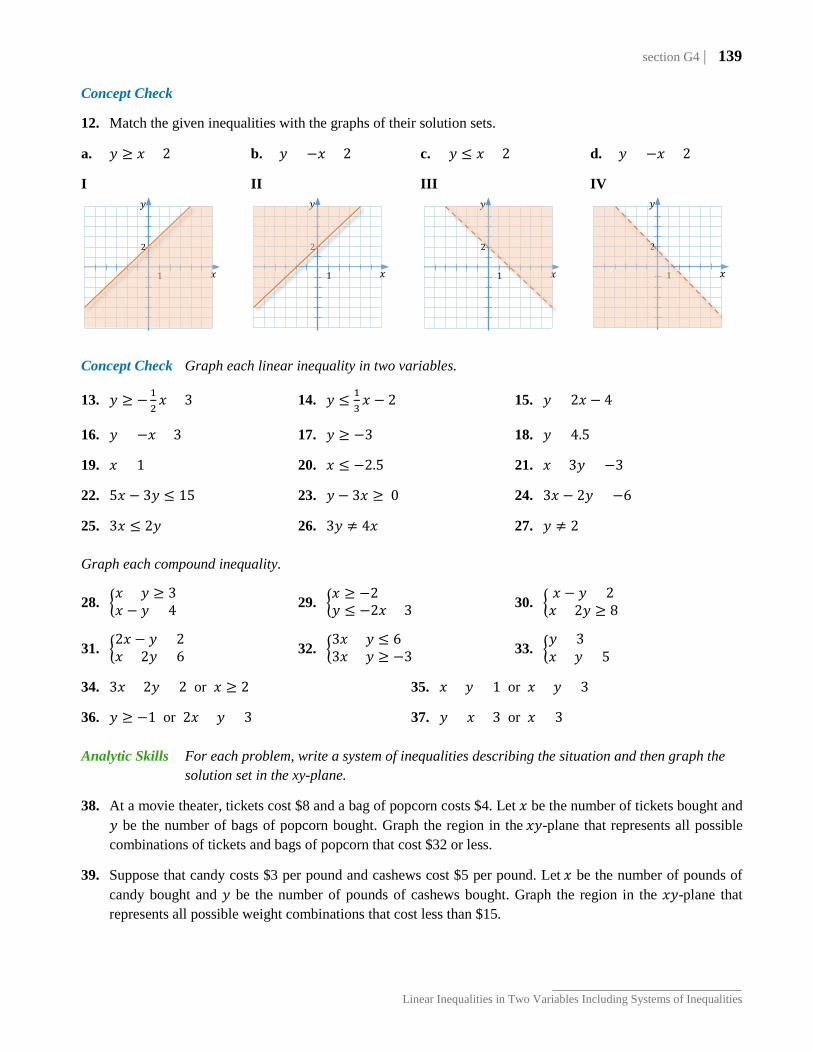
section G4 | 139


Concept Check

12. Match the given inequalities with the graphs of their solution sets.

a. 𝑦𝑦 ≥ 𝑥𝑥 + 2 b. 𝑦𝑦 < −𝑥𝑥 + 2 c. 𝑦𝑦 ≤ 𝑥𝑥 + 2 d. 𝑦𝑦 > −𝑥𝑥 + 2

I II III IV

Concept Check Graph each linear inequality in two variables.

13. 𝑦𝑦 ≥ −12𝑥𝑥 + 3 14. 𝑦𝑦 ≤ 1

3𝑥𝑥 − 2 15. 𝑦𝑦 < 2𝑥𝑥 − 4

16. 𝑦𝑦 > −𝑥𝑥 + 3 17. 𝑦𝑦 ≥ −3 18. 𝑦𝑦 < 4.5

19. 𝑥𝑥 > 1 20. 𝑥𝑥 ≤ −2.5 21. 𝑥𝑥 + 3𝑦𝑦 > −3

22. 5𝑥𝑥 − 3𝑦𝑦 ≤ 15 23. 𝑦𝑦 − 3𝑥𝑥 ≥ 0 24. 3𝑥𝑥 − 2𝑦𝑦 < −6

25. 3𝑥𝑥 ≤ 2𝑦𝑦 26. 3𝑦𝑦 ≠ 4𝑥𝑥 27. 𝑦𝑦 ≠ 2 Graph each compound inequality.

28. �𝑥𝑥 + 𝑦𝑦 ≥ 3𝑥𝑥 − 𝑦𝑦 < 4 29. �𝑥𝑥 ≥ −2

𝑦𝑦 ≤ −2𝑥𝑥 + 3 30. � 𝑥𝑥 − 𝑦𝑦 < 2𝑥𝑥 + 2𝑦𝑦 ≥ 8

31. �2𝑥𝑥 − 𝑦𝑦 < 2𝑥𝑥 + 2𝑦𝑦 > 6 32. �3𝑥𝑥 + 𝑦𝑦 ≤ 6

3𝑥𝑥 + 𝑦𝑦 ≥ −3 33. �𝑦𝑦 < 3𝑥𝑥 + 𝑦𝑦 < 5

34. 3𝑥𝑥 + 2𝑦𝑦 > 2 or 𝑥𝑥 ≥ 2 35. 𝑥𝑥 + 𝑦𝑦 > 1 or 𝑥𝑥 + 𝑦𝑦 < 3

36. 𝑦𝑦 ≥ −1 or 2𝑥𝑥 + 𝑦𝑦 > 3 37. 𝑦𝑦 > 𝑥𝑥 + 3 or 𝑥𝑥 > 3

Analytic Skills For each problem, write a system of inequalities describing the situation and then graph the solution set in the xy-plane.

38. At a movie theater, tickets cost $8 and a bag of popcorn costs $4. Let 𝑥𝑥 be the number of tickets bought and 𝑦𝑦 be the number of bags of popcorn bought. Graph the region in the 𝑥𝑥𝑦𝑦-plane that represents all possible combinations of tickets and bags of popcorn that cost $32 or less.

39. Suppose that candy costs $3 per pound and cashews cost $5 per pound. Let 𝑥𝑥 be the number of pounds of candy bought and 𝑦𝑦 be the number of pounds of cashews bought. Graph the region in the 𝑥𝑥𝑦𝑦-plane that represents all possible weight combinations that cost less than $15.

𝑦𝑦

𝑥𝑥

2

1

𝑦𝑦

𝑥𝑥

2

1

𝑦𝑦

𝑥𝑥

2

1

𝑦𝑦

𝑥𝑥

2

1

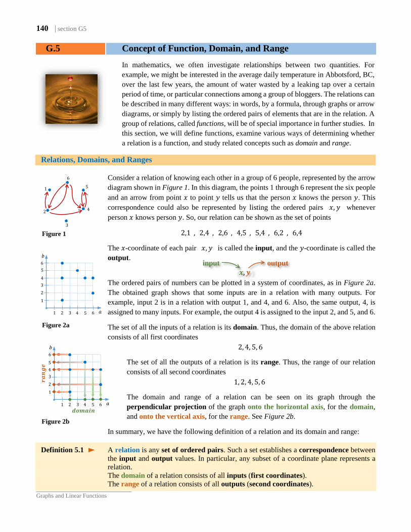
140 | section G5


G.5 Concept of Function, Domain, and Range

In mathematics, we often investigate relationships between two quantities. For example, we might be interested in the average daily temperature in Abbotsford, BC, over the last few years, the amount of water wasted by a leaking tap over a certain period of time, or particular connections among a group of bloggers. The relations can be described in many different ways: in words, by a formula, through graphs or arrow diagrams, or simply by listing the ordered pairs of elements that are in the relation. A group of relations, called functions, will be of special importance in further studies. In this section, we will define functions, examine various ways of determining whether a relation is a function, and study related concepts such as domain and range.

Relations, Domains, and Ranges

Consider a relation of knowing each other in a group of 6 people, represented by the arrow diagram shown in Figure 1. In this diagram, the points 1 through 6 represent the six people and an arrow from point 𝑥𝑥 to point 𝑦𝑦 tells us that the person 𝑥𝑥 knows the person 𝑦𝑦. This correspondence could also be represented by listing the ordered pairs (𝑥𝑥, 𝑦𝑦) whenever person 𝑥𝑥 knows person 𝑦𝑦. So, our relation can be shown as the set of points

{(2,1), (2,4), (2,6), (4,5), (5,4), (6,2), (6,4)}

The 𝑥𝑥-coordinate of each pair (𝑥𝑥,𝑦𝑦) is called the input, and the 𝑦𝑦-coordinate is called the output.

The ordered pairs of numbers can be plotted in a system of coordinates, as in Figure 2a. The obtained graph shows that some inputs are in a relation with many outputs. For example, input 2 is in a relation with output 1, and 4, and 6. Also, the same output, 4, is assigned to many inputs. For example, the output 4 is assigned to the input 2, and 5, and 6.

The set of all the inputs of a relation is its domain. Thus, the domain of the above relation consists of all first coordinates

{ 2, 4, 5, 6}

The set of all the outputs of a relation is its range. Thus, the range of our relation consists of all second coordinates

{1, 2, 4, 5, 6}

The domain and range of a relation can be seen on its graph through the perpendicular projection of the graph onto the horizontal axis, for the domain, and onto the vertical axis, for the range. See Figure 2b.

In summary, we have the following definition of a relation and its domain and range:

Definition 5.1 A relation is any set of ordered pairs. Such a set establishes a correspondence between the input and output values. In particular, any subset of a coordinate plane represents a relation.

The domain of a relation consists of all inputs (first coordinates). The range of a relation consists of all outputs (second coordinates).

Figure 2a

3

2 4

5

6

1

6

2

3

5

5

𝑏𝑏

𝑎𝑎

1

4

4

1 6 3 2

𝒓𝒓𝒓𝒓𝒓𝒓𝒓𝒓

𝒓𝒓

𝒅𝒅𝒅𝒅𝒅𝒅𝒓𝒓𝒅𝒅𝒓𝒓

6

2

3

5

5

𝑏𝑏

𝑎𝑎

1

4

4

1 6 3 2

Figure 1

Figure 2b

input output (𝑨𝑨,𝑩𝑩)

section G5 | 141

Concept of Function, Domain, and Range

Relations can also be given by an equation or an inequality. For example, the equation

|𝑦𝑦| = |𝑥𝑥|

describes the set of points in the 𝑥𝑥𝑦𝑦-plane that lie on two diagonals, 𝑦𝑦 = 𝑥𝑥 and 𝑦𝑦 = −𝑥𝑥. In this case, the domain and range for this relation are both the set of real numbers because the projection of the graph onto each axis covers the entire axis.

Functions, Domains, and Ranges Relations that have exactly one output for every input are of special importance in mathematics. This is because as long as we know the rule of a correspondence defining the relation, the output can be uniquely determined for every input. Such relations are called functions. For example, the linear equation 𝑦𝑦 = 2𝑥𝑥 + 1 defines a function, as for every input 𝑥𝑥, one can calculate the corresponding 𝑦𝑦-value in a unique way. Since both the input and the output can be any real number, the domain and range of this function are both the set of real numbers.

Definition 5.2 A function is a relation that assigns exactly one output value in the range to each input value of the domain.

If (𝑥𝑥,𝑦𝑦) is an ordered pair that belongs to a function, then 𝑥𝑥 can be any arbitrarily chosen input value of the domain of this function, while 𝑦𝑦 must be the uniquely determined value that is assigned to 𝑥𝑥 by this function. That is why 𝑥𝑥 is referred to as an independent variable while 𝑦𝑦 is referred to as the dependent variable (because the 𝑦𝑦-value depends on the chosen 𝑥𝑥-value).

How can we recognize if a relation is a function?

If the relation is given as a set of ordered pairs, it is enough to check if there are no two pairs with the same inputs. For example:

{(2,1), (2,4), (1,3)} {(2,1), (1,3), (4,1)} relation function

If the relation is given by a diagram, we want to check if no point from the domain is assigned to two points in the range. For example:

𝑦𝑦

𝑥𝑥 1

1

independent variable

dependent variable (𝑨𝑨,𝑩𝑩)

The pairs (2,1) and (2,4) have the same inputs. So, there are two 𝑩𝑩-values assigned to the 𝑥𝑥-value 2,

which makes it not a function.

There are no pairs with the same inputs, so each 𝑥𝑥-value is associated with exactly

one pair and consequently with exactly one 𝑦𝑦-value. This makes it a function.

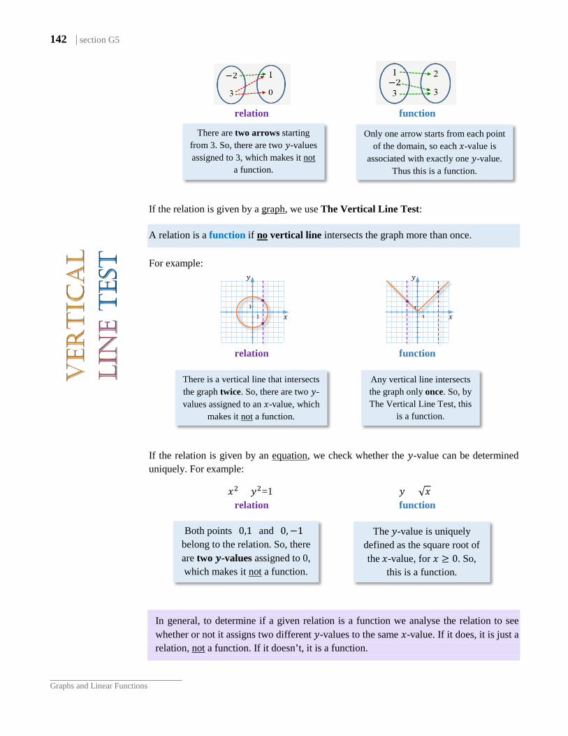
142 | section G5


relation function

If the relation is given by a graph, we use The Vertical Line Test:

A relation is a function if no vertical line intersects the graph more than once.

For example:

relation function

If the relation is given by an equation, we check whether the 𝑦𝑦-value can be determined uniquely. For example:

𝑥𝑥2 + 𝑦𝑦2=1 𝑦𝑦 = √𝑥𝑥 relation function

In general, to determine if a given relation is a function we analyse the relation to see whether or not it assigns two different 𝑦𝑦-values to the same 𝑥𝑥-value. If it does, it is just a relation, not a function. If it doesn’t, it is a function.

𝑦𝑦

𝑥𝑥 1

1

𝑦𝑦

𝑥𝑥 1

1

Both points (0,1) and (0,−1) belong to the relation. So, there are two 𝑩𝑩-values assigned to 0, which makes it not a function.

The 𝑦𝑦-value is uniquely defined as the square root of the 𝑥𝑥-value, for 𝑥𝑥 ≥ 0. So,

this is a function.

There are two arrows starting from 3. So, there are two 𝑦𝑦-values assigned to 3, which makes it not

a function.

Only one arrow starts from each point of the domain, so each 𝑥𝑥-value is

associated with exactly one 𝑦𝑦-value. Thus this is a function.

There is a vertical line that intersects the graph twice. So, there are two 𝑦𝑦-values assigned to an 𝑥𝑥-value, which

makes it not a function.

Any vertical line intersects the graph only once. So, by The Vertical Line Test, this

is a function.

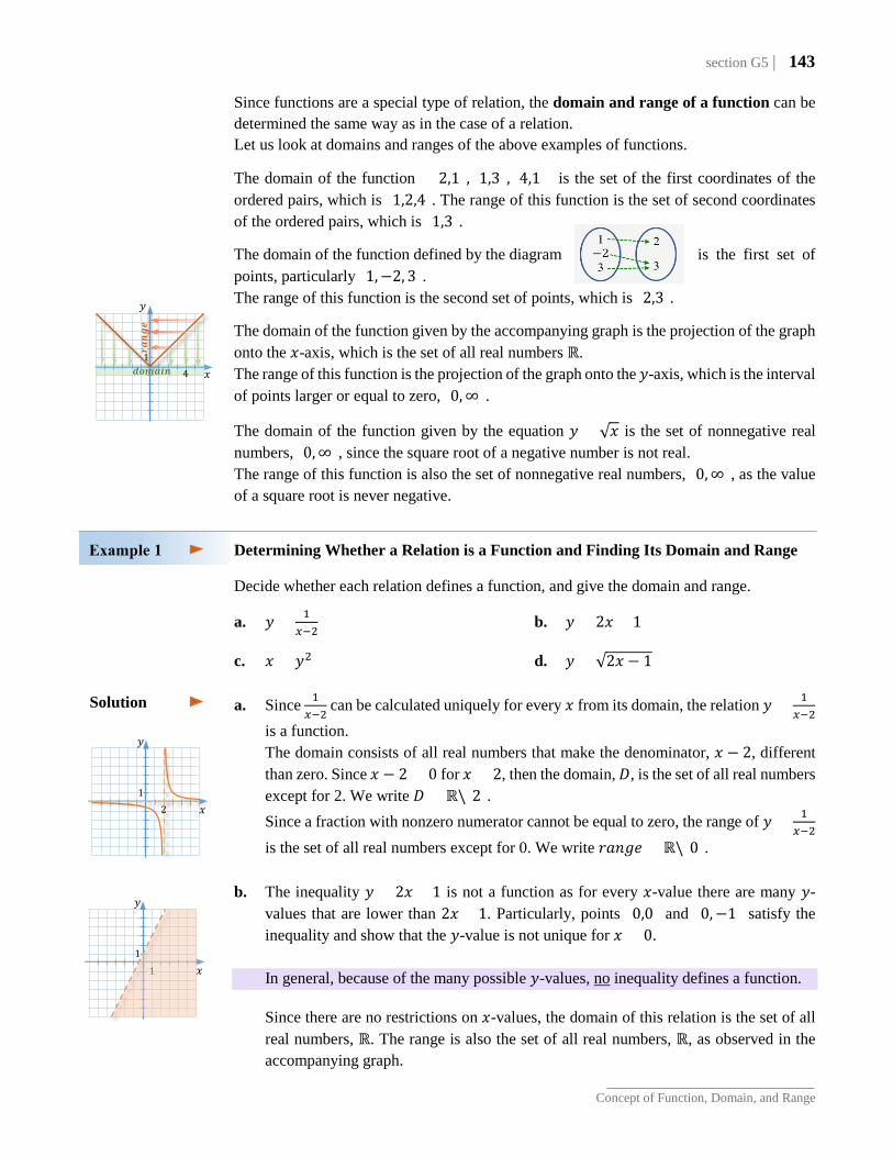
section G5 | 143


Since functions are a special type of relation, the domain and range of a function can be determined the same way as in the case of a relation. Let us look at domains and ranges of the above examples of functions.

The domain of the function {(2,1), (1,3), (4,1)} is the set of the first coordinates of the ordered pairs, which is {1,2,4}. The range of this function is the set of second coordinates of the ordered pairs, which is {1,3}.

The domain of the function defined by the diagram is the first set of points, particularly {1,−2, 3}. The range of this function is the second set of points, which is {2,3}.

The domain of the function given by the accompanying graph is the projection of the graph onto the 𝑥𝑥-axis, which is the set of all real numbers ℝ. The range of this function is the projection of the graph onto the 𝑦𝑦-axis, which is the interval of points larger or equal to zero, [0,∞).

The domain of the function given by the equation 𝑦𝑦 = √𝑥𝑥 is the set of nonnegative real numbers, [0,∞), since the square root of a negative number is not real. The range of this function is also the set of nonnegative real numbers, [0,∞), as the value of a square root is never negative.

Determining Whether a Relation is a Function and Finding Its Domain and Range Decide whether each relation defines a function, and give the domain and range.

a. 𝑦𝑦 = 1𝑥𝑥−2

b. 𝑦𝑦 < 2𝑥𝑥 + 1

c. 𝑥𝑥 = 𝑦𝑦2 d. 𝑦𝑦 = √2𝑥𝑥 − 1

a. Since 1𝑥𝑥−2

can be calculated uniquely for every 𝑥𝑥 from its domain, the relation 𝑦𝑦 = 1𝑥𝑥−2

is a function.

The domain consists of all real numbers that make the denominator, 𝑥𝑥 − 2, different than zero. Since 𝑥𝑥 − 2 = 0 for 𝑥𝑥 = 2, then the domain, 𝐷𝐷, is the set of all real numbers except for 2. We write 𝐷𝐷 = ℝ\{2}.

Since a fraction with nonzero numerator cannot be equal to zero, the range of 𝑦𝑦 = 1𝑥𝑥−2

is the set of all real numbers except for 0. We write 𝑟𝑟𝑎𝑎𝑝𝑝𝑟𝑟𝑡𝑡 = ℝ\{0}.

b. The inequality 𝑦𝑦 < 2𝑥𝑥 + 1 is not a function as for every 𝑥𝑥-value there are many 𝑦𝑦-

values that are lower than 2𝑥𝑥 + 1. Particularly, points (0,0) and (0,−1) satisfy the inequality and show that the 𝑦𝑦-value is not unique for 𝑥𝑥 = 0.

In general, because of the many possible 𝑦𝑦-values, no inequality defines a function.

Since there are no restrictions on 𝑥𝑥-values, the domain of this relation is the set of all real numbers, ℝ. The range is also the set of all real numbers, ℝ, as observed in the accompanying graph.

Solution

𝑦𝑦

𝑥𝑥 1

1

𝑦𝑦

𝑥𝑥 1

2

𝑦𝑦

𝑥𝑥 1

4 𝒅𝒅𝒅𝒅𝒅𝒅𝒓𝒓𝒅𝒅𝒓𝒓


𝒓𝒓

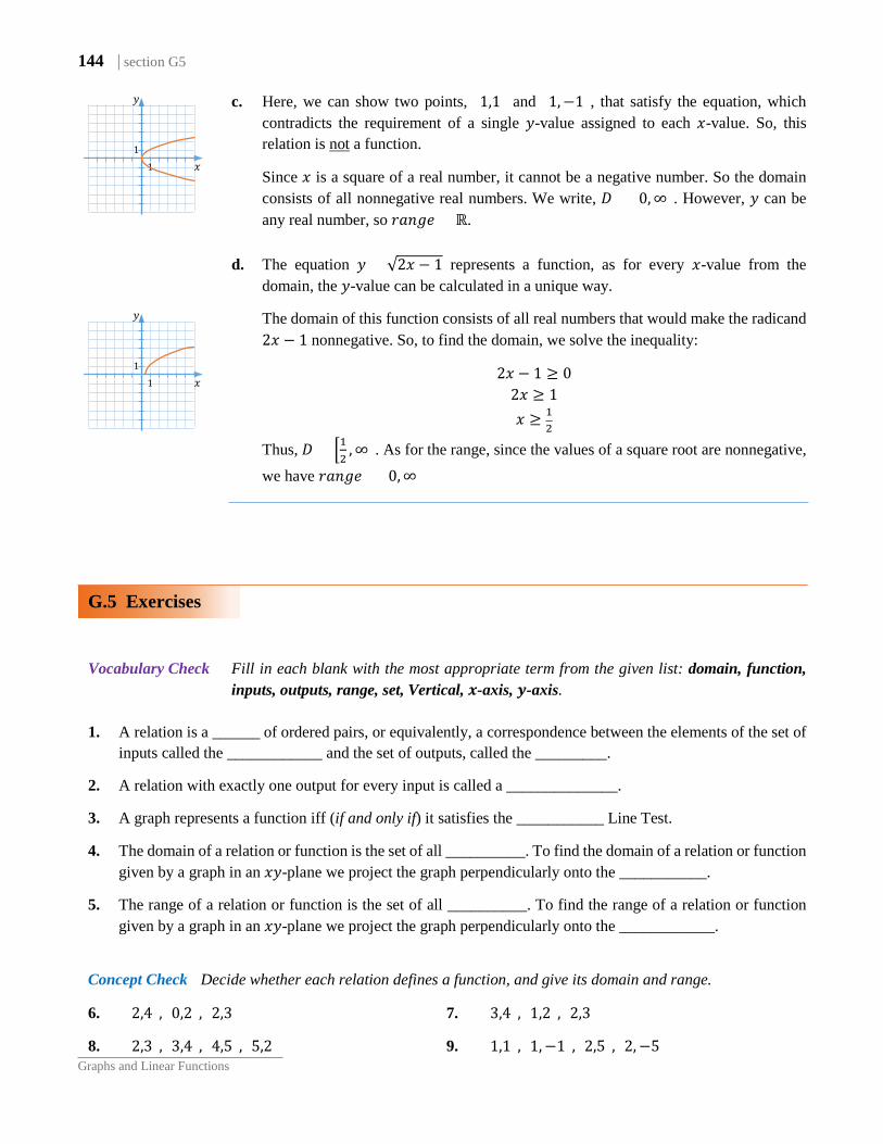
144 | section G5


c. Here, we can show two points, (1,1) and (1,−1), that satisfy the equation, which contradicts the requirement of a single 𝑦𝑦-value assigned to each 𝑥𝑥-value. So, this relation is not a function.

Since 𝑥𝑥 is a square of a real number, it cannot be a negative number. So the domain consists of all nonnegative real numbers. We write, 𝐷𝐷 = [0,∞). However, 𝑦𝑦 can be any real number, so 𝑟𝑟𝑎𝑎𝑝𝑝𝑟𝑟𝑡𝑡 = ℝ.

d. The equation 𝑦𝑦 = √2𝑥𝑥 − 1 represents a function, as for every 𝑥𝑥-value from the

domain, the 𝑦𝑦-value can be calculated in a unique way.

The domain of this function consists of all real numbers that would make the radicand 2𝑥𝑥 − 1 nonnegative. So, to find the domain, we solve the inequality:

2𝑥𝑥 − 1 ≥ 0 2𝑥𝑥 ≥ 1 𝑥𝑥 ≥ 1

2

Thus, 𝐷𝐷 = �12

,∞). As for the range, since the values of a square root are nonnegative,

we have 𝑟𝑟𝑎𝑎𝑝𝑝𝑟𝑟𝑡𝑡 = [0,∞)

G.5 Exercises

Vocabulary Check Fill in each blank with the most appropriate term from the given list: domain, function, inputs, outputs, range, set, Vertical, 𝑨𝑨-axis, 𝑩𝑩-axis.

1. A relation is a ______ of ordered pairs, or equivalently, a correspondence between the elements of the set of

inputs called the ____________ and the set of outputs, called the _________.

2. A relation with exactly one output for every input is called a ______________.

3. A graph represents a function iff (if and only if) it satisfies the ___________ Line Test.

4. The domain of a relation or function is the set of all __________. To find the domain of a relation or function given by a graph in an 𝑥𝑥𝑦𝑦-plane we project the graph perpendicularly onto the ___________.

5. The range of a relation or function is the set of all __________. To find the range of a relation or function given by a graph in an 𝑥𝑥𝑦𝑦-plane we project the graph perpendicularly onto the ____________.

Concept Check Decide whether each relation defines a function, and give its domain and range.

6. {(2,4), (0,2), (2,3)} 7. {(3,4), (1,2), (2,3)}

8. {(2,3), (3,4), (4,5), (5,2)} 9. {(1,1), (1,−1), (2,5), (2,−5)}

𝑦𝑦

𝑥𝑥 1

1

𝑦𝑦

𝑥𝑥 1

1

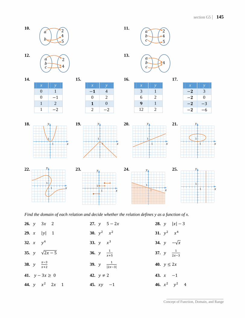
section G5 | 145


10. 11.

12. 13.

14. 15. 16. 17.

18. 19. 20. 21.

22. 23. 24. 25.

Find the domain of each relation and decide whether the relation defines y as a function of x.

26. 𝑦𝑦 = 3𝑥𝑥 + 2 27. 𝑦𝑦 = 5 − 2𝑥𝑥 28. 𝑦𝑦 = |𝑥𝑥| − 3

29. 𝑥𝑥 = |𝑦𝑦| + 1 30. 𝑦𝑦2 = 𝑥𝑥2 31. 𝑦𝑦2 = 𝑥𝑥4

32. 𝑥𝑥 = 𝑦𝑦4 33. 𝑦𝑦 = 𝑥𝑥3 34. 𝑦𝑦 = −√𝑥𝑥

35. 𝑦𝑦 = √2𝑥𝑥 − 5 36. 𝑦𝑦 = 1𝑥𝑥+5

37. 𝑦𝑦 = 12𝑥𝑥−3

38. 𝑦𝑦 = 𝑥𝑥−3𝑥𝑥+2

39. 𝑦𝑦 = 1|2𝑥𝑥−3| 40. 𝑦𝑦 ≤ 2𝑥𝑥

41. 𝑦𝑦 − 3𝑥𝑥 ≥ 0 42. 𝑦𝑦 ≠ 2 43. 𝑥𝑥 = −1

44. 𝑦𝑦 = 𝑥𝑥2 + 2𝑥𝑥 + 1 45. 𝑥𝑥𝑦𝑦 = −1 46. 𝑥𝑥2 + 𝑦𝑦2 = 4

x y −𝟏𝟏 4 0 2 𝟏𝟏 0 2 −2

x y 3 1 6 2 𝟗𝟗 1 12 2

x y −𝟐𝟐 3 −𝟐𝟐 0 −𝟐𝟐 −3 −𝟐𝟐 −6

x y 0 1 0 −1 1 2 1 −2

𝑏𝑏

𝑎𝑎

5

2 4 𝑏𝑏

𝑎𝑎

5

2 4

𝑐𝑐

𝑏𝑏 𝑎𝑎

4 𝑐𝑐

𝑏𝑏 𝑎𝑎 2

4 𝑐𝑐

𝑦𝑦

𝑥𝑥

1

1

𝑦𝑦

𝑥𝑥

1

1

𝑦𝑦

𝑥𝑥

1

1

𝑦𝑦

𝑥𝑥

1

1

𝑦𝑦

𝑥𝑥

1

1

𝑦𝑦

𝑥𝑥

1

1

𝑦𝑦

𝑥𝑥

1

1

𝑦𝑦

𝑥𝑥 1

1

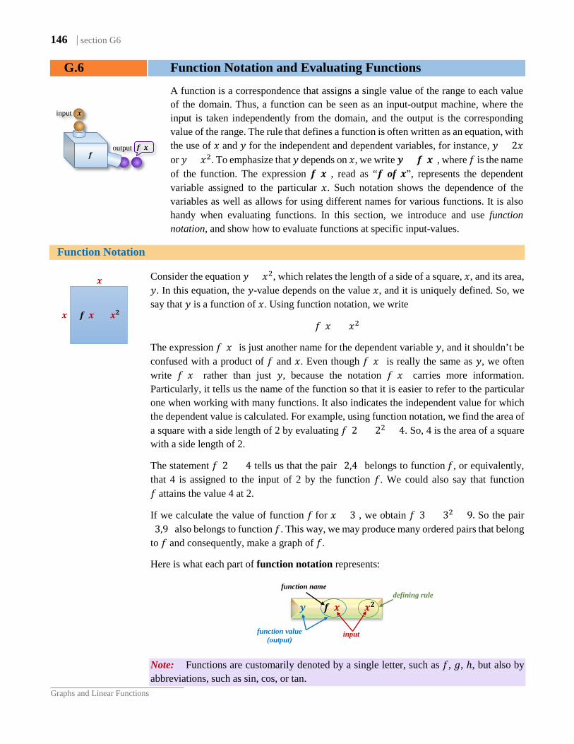
146 | section G6


G.6 Function Notation and Evaluating Functions

A function is a correspondence that assigns a single value of the range to each value of the domain. Thus, a function can be seen as an input-output machine, where the input is taken independently from the domain, and the output is the corresponding value of the range. The rule that defines a function is often written as an equation, with the use of 𝑥𝑥 and 𝑦𝑦 for the independent and dependent variables, for instance, 𝑦𝑦 = 2𝑥𝑥 or 𝑦𝑦 = 𝑥𝑥2. To emphasize that 𝑦𝑦 depends on 𝑥𝑥, we write 𝑩𝑩 = 𝒇𝒇(𝑨𝑨), where 𝑓𝑓 is the name of the function. The expression 𝒇𝒇(𝑨𝑨), read as “𝒇𝒇 of 𝑨𝑨”, represents the dependent variable assigned to the particular 𝑥𝑥. Such notation shows the dependence of the variables as well as allows for using different names for various functions. It is also handy when evaluating functions. In this section, we introduce and use function notation, and show how to evaluate functions at specific input-values.

Function Notation

Consider the equation 𝑦𝑦 = 𝑥𝑥2, which relates the length of a side of a square, 𝑥𝑥, and its area, 𝑦𝑦. In this equation, the 𝑦𝑦-value depends on the value 𝑥𝑥, and it is uniquely defined. So, we say that 𝑦𝑦 is a function of 𝑥𝑥. Using function notation, we write

𝑓𝑓(𝑥𝑥) = 𝑥𝑥2

The expression 𝑓𝑓(𝑥𝑥) is just another name for the dependent variable 𝑦𝑦, and it shouldn’t be confused with a product of 𝑓𝑓 and 𝑥𝑥. Even though 𝑓𝑓(𝑥𝑥) is really the same as 𝑦𝑦, we often write 𝑓𝑓(𝑥𝑥) rather than just 𝑦𝑦, because the notation 𝑓𝑓(𝑥𝑥) carries more information. Particularly, it tells us the name of the function so that it is easier to refer to the particular one when working with many functions. It also indicates the independent value for which the dependent value is calculated. For example, using function notation, we find the area of a square with a side length of 2 by evaluating 𝑓𝑓(2) = 22 = 4. So, 4 is the area of a square with a side length of 2.

The statement 𝑓𝑓(2) = 4 tells us that the pair (2,4) belongs to function 𝑓𝑓, or equivalently, that 4 is assigned to the input of 2 by the function 𝑓𝑓. We could also say that function 𝑓𝑓 attains the value 4 at 2.

If we calculate the value of function 𝑓𝑓 for 𝑥𝑥 = 3 , we obtain 𝑓𝑓(3) = 32 = 9. So the pair (3,9) also belongs to function 𝑓𝑓. This way, we may produce many ordered pairs that belong to 𝑓𝑓 and consequently, make a graph of 𝑓𝑓.

Here is what each part of function notation represents:

𝑩𝑩 = 𝒇𝒇(𝑨𝑨) = 𝑨𝑨𝟐𝟐

Note: Functions are customarily denoted by a single letter, such as 𝑓𝑓, 𝑟𝑟, ℎ, but also by abbreviations, such as sin, cos, or tan.

function name

input function value (output)

defining rule

𝑨𝑨

𝑨𝑨 𝒇𝒇(𝑨𝑨) = 𝑨𝑨𝟐𝟐

input 𝑨𝑨

𝒇𝒇(𝑨𝑨) 𝒇𝒇

output

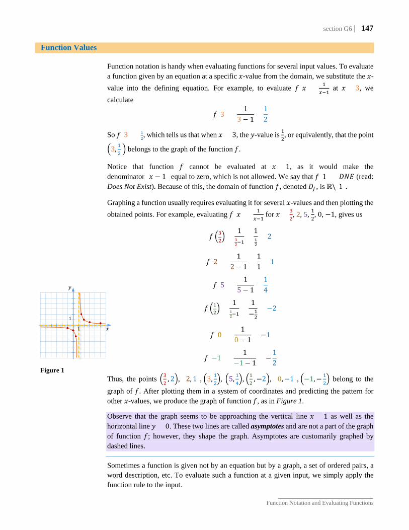
section G6 | 147

Function Notation and Evaluating Functions

Function Values Function notation is handy when evaluating functions for several input values. To evaluate a function given by an equation at a specific 𝑥𝑥-value from the domain, we substitute the 𝑥𝑥-value into the defining equation. For example, to evaluate 𝑓𝑓(𝑥𝑥) = 1

𝑥𝑥−1 at 𝑥𝑥 = 3, we

calculate

𝑓𝑓(3) =1

3 − 1=

12

So 𝑓𝑓(3) = 12, which tells us that when 𝑥𝑥 = 3, the 𝑦𝑦-value is 1

2, or equivalently, that the point

�3, 12 � belongs to the graph of the function 𝑓𝑓.

Notice that function 𝑓𝑓 cannot be evaluated at 𝑥𝑥 = 1, as it would make the denominator (𝑥𝑥 − 1) equal to zero, which is not allowed. We say that 𝑓𝑓(1) = 𝐷𝐷𝐷𝐷𝐷𝐷 (read: Does Not Exist). Because of this, the domain of function 𝑓𝑓, denoted 𝐷𝐷𝑓𝑓, is ℝ\{1}.

Graphing a function usually requires evaluating it for several 𝑥𝑥-values and then plotting the obtained points. For example, evaluating 𝑓𝑓(𝑥𝑥) = 1

𝑥𝑥−1 for 𝑥𝑥 = 3

2, 2, 5, 1

2, 0, −1, gives us

𝑓𝑓 �32� =

132−1

=112

= 2

𝑓𝑓(2) =1

2 − 1=

11

= 1

𝑓𝑓(5) =1

5 − 1=

14

𝑓𝑓 �12� =

112−1

=1−12

= −2

𝑓𝑓(0) =1

0 − 1= −1

𝑓𝑓(−1) =1

−1− 1= −

12

Thus, the points �32

, 2�, (2, 1), �3, 12�, �5, 1

4�, �1

2,−2�, (0,−1), �−1,−1

2� belong to the

graph of 𝑓𝑓. After plotting them in a system of coordinates and predicting the pattern for other 𝑥𝑥-values, we produce the graph of function 𝑓𝑓, as in Figure 1.

Observe that the graph seems to be approaching the vertical line 𝑥𝑥 = 1 as well as the horizontal line 𝑦𝑦 = 0. These two lines are called asymptotes and are not a part of the graph of function 𝑓𝑓; however, they shape the graph. Asymptotes are customarily graphed by dashed lines. Sometimes a function is given not by an equation but by a graph, a set of ordered pairs, a word description, etc. To evaluate such a function at a given input, we simply apply the function rule to the input.

Figure 1

𝑦𝑦

𝑥𝑥

1

1

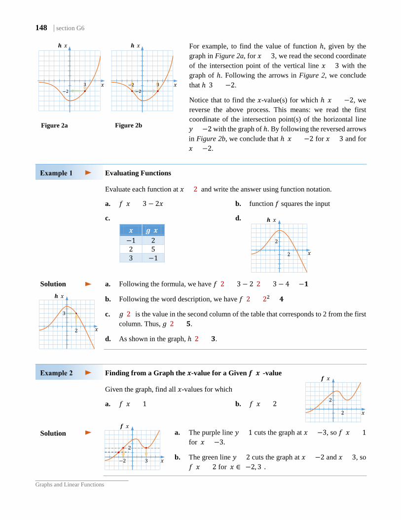
148 | section G6


For example, to find the value of function ℎ, given by the graph in Figure 2a, for 𝑥𝑥 = 3, we read the second coordinate of the intersection point of the vertical line 𝑥𝑥 = 3 with the graph of ℎ. Following the arrows in Figure 2, we conclude that ℎ(3) = −2.

Notice that to find the 𝑥𝑥-value(s) for which ℎ(𝑥𝑥) = −2, we reverse the above process. This means: we read the first coordinate of the intersection point(s) of the horizontal line 𝑦𝑦 = −2 with the graph of ℎ. By following the reversed arrows in Figure 2b, we conclude that ℎ(𝑥𝑥) = −2 for 𝑥𝑥 = 3 and for 𝑥𝑥 = −2.

Evaluating Functions Evaluate each function at 𝑥𝑥 = 2 and write the answer using function notation.

a. 𝑓𝑓(𝑥𝑥) = 3 − 2𝑥𝑥 b. function 𝑓𝑓 squares the input

c. d.

a. Following the formula, we have 𝑓𝑓(2) = 3 − 2(2) = 3 − 4 = −𝟏𝟏

b. Following the word description, we have 𝑓𝑓(2) = 22 = 𝟒𝟒

c. 𝑟𝑟(2) is the value in the second column of the table that corresponds to 2 from the first column. Thus, 𝑟𝑟(2) = 𝟓𝟓.

d. As shown in the graph, ℎ(2) = 𝟑𝟑.

Finding from a Graph the 𝑨𝑨-value for a Given 𝒇𝒇(𝑨𝑨)-value Given the graph, find all 𝑥𝑥-values for which

a. 𝑓𝑓(𝑥𝑥) = 1 b. 𝑓𝑓(𝑥𝑥) = 2

a. The purple line 𝑦𝑦 = 1 cuts the graph at 𝑥𝑥 = −3, so 𝑓𝑓(𝑥𝑥) = 1 for 𝑥𝑥 = −3.

b. The green line 𝑦𝑦 = 2 cuts the graph at 𝑥𝑥 = −2 and 𝑥𝑥 = 3, so 𝑓𝑓(𝑥𝑥) = 2 for 𝑥𝑥 ∈ {−2, 3}.

𝑨𝑨 𝒓𝒓(𝑨𝑨) −1 2 2 5 3 −1

Solution

Figure 2a

Solution

𝒉𝒉(𝑥𝑥)

𝑥𝑥 2

2

𝒉𝒉(𝑥𝑥)

𝑥𝑥 −2

3

Figure 2b

𝒉𝒉(𝑥𝑥)

𝑥𝑥 −2

3 −2

𝒉𝒉(𝑥𝑥)

𝑥𝑥 2

3

𝒇𝒇(𝑥𝑥)

𝑥𝑥 2

2

𝒇𝒇(𝑥𝑥)

𝑥𝑥 3

2

−2

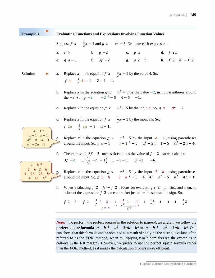
section G6 | 149


Evaluating Functions and Expressions Involving Function Values

Suppose 𝑓𝑓(𝑥𝑥) = 12𝑥𝑥 − 1 and 𝑟𝑟(𝑥𝑥) = 𝑥𝑥2 − 5. Evaluate each expression.

a. 𝑓𝑓(4) b. 𝑟𝑟(−2) c. 𝑟𝑟(𝑎𝑎) d. 𝑓𝑓(2𝑎𝑎)

e. 𝑟𝑟(𝑎𝑎 − 1) f. 3𝑓𝑓(−2) g. 𝑟𝑟(2 + ℎ) h. 𝑓𝑓(2 + ℎ) − 𝑓𝑓(2)

a. Replace 𝑥𝑥 in the equation 𝑓𝑓(𝑥𝑥) = 12𝑥𝑥 − 1 by the value 4. So,

𝑓𝑓(4) = 12

(4) − 1 = 2 − 1 = 𝟏𝟏. b. Replace 𝑥𝑥 in the equation 𝑟𝑟(𝑥𝑥) = 𝑥𝑥2 − 5 by the value −2, using parentheses around

the −2. So, 𝑟𝑟(−2) = (−2)2 − 5 = 4 − 5 = −𝟏𝟏. c. Replace 𝑥𝑥 in the equation 𝑟𝑟(𝑥𝑥) = 𝑥𝑥2 − 5 by the input 𝑎𝑎. So, 𝑟𝑟(𝑎𝑎) = 𝒓𝒓𝟐𝟐 − 𝟓𝟓. d. Replace 𝑥𝑥 in the equation 𝑓𝑓(𝑥𝑥) = 1

2𝑥𝑥 − 1 by the input 2𝑎𝑎. So,

𝑓𝑓(2𝑎𝑎) = 12

(2𝑎𝑎) − 1 = 𝒓𝒓 − 𝟏𝟏. e. Replace 𝑥𝑥 in the equation 𝑟𝑟(𝑥𝑥) = 𝑥𝑥2 − 5 by the input (𝑎𝑎 − 1), using parentheses

around the input. So, 𝑟𝑟(𝑎𝑎 − 1) = (𝑎𝑎 − 1)2 − 5 = 𝑎𝑎2 − 2𝑎𝑎 + 1 − 5 = 𝒓𝒓𝟐𝟐 − 𝟐𝟐𝒓𝒓 − 𝟒𝟒. f. The expression 3𝑓𝑓(−2) means three times the value of 𝑓𝑓(−2), so we calculate

3𝑓𝑓(−2) = 3 ∙ �12

(−2) − 1� = 3(−1 − 1) = 3(−2) = −𝟔𝟔. g. Replace 𝑥𝑥 in the equation 𝑟𝑟(𝑥𝑥) = 𝑥𝑥2 − 5 by the input (2 + ℎ), using parentheses

around the input. So, 𝑟𝑟(2 + ℎ) = (2 + ℎ)2 − 5 = 4 + 4ℎ + ℎ2 − 5 = 𝒉𝒉𝟐𝟐 + 𝟒𝟒𝒉𝒉 − 𝟏𝟏. h. When evaluating 𝑓𝑓(2 + ℎ) − 𝑓𝑓(2), focus on evaluating 𝑓𝑓(2 + ℎ) first and then, to

subtract the expression 𝑓𝑓(2), use a bracket just after the subtraction sign. So,

𝑓𝑓(2 + ℎ) − 𝑓𝑓(2) = 12

(2 + ℎ) − 1��𝑓𝑓(2+ℎ)

− �12

(2) − 1��𝑓𝑓(2)

= 1 + 12ℎ − 1 − [1 − 1] = 𝟏𝟏

𝟐𝟐𝒉𝒉

Note: To perform the perfect squares in the solution to Example 3e and 3g, we follow the perfect square formula (𝒓𝒓 + 𝒃𝒃)𝟐𝟐 = 𝒓𝒓𝟐𝟐 + 𝟐𝟐𝒓𝒓𝒃𝒃 + 𝒃𝒃𝟐𝟐 or (𝒓𝒓 − 𝒃𝒃)𝟐𝟐 = 𝒓𝒓𝟐𝟐 − 𝟐𝟐𝒓𝒓𝒃𝒃 + 𝒃𝒃𝟐𝟐. One can check that this formula can be obtained as a result of applying the distributive law, often referred to as the FOIL method, when multiplying two binomials (see the examples in callouts in the left margin). However, we prefer to use the perfect square formula rather than the FOIL method, as it makes the calculation process more efficient.

Solution

(𝑎𝑎 − 1)2

= (𝑎𝑎 − 1)(𝑎𝑎 − 1)= 𝑎𝑎2 − 𝑎𝑎 − 𝑎𝑎 + 1= 𝑎𝑎2 − 2𝑎𝑎 + 1

(2 + ℎ)2

= (2 + ℎ)(2 + ℎ) = 4 + 2ℎ + 2ℎ + ℎ2

= 4 + 4ℎ + ℎ2

150 | section G6


Function Notation in Graphing and Application Problems

By Definition 1.1 in section G1, a linear equation is an equation of the form 𝐴𝐴𝑥𝑥 + 𝐵𝐵𝑦𝑦 = 𝐶𝐶. The graph of any linear equation is a line, and any nonvertical line satisfies the Vertical Line Test. Thus, any linear equation 𝐴𝐴𝑥𝑥 + 𝐵𝐵𝑦𝑦 = 𝐶𝐶 with 𝐵𝐵 ≠ 0 defines a linear function.

How can we write this function using function notation?

Since 𝑦𝑦 = 𝑓𝑓(𝑥𝑥), we can replace the variable 𝑦𝑦 in the equation 𝐴𝐴𝑥𝑥 + 𝐵𝐵𝑦𝑦 = 𝐶𝐶 with 𝑓𝑓(𝑥𝑥) and then solve for 𝑓𝑓(𝑥𝑥). So, we obtain

𝐴𝐴𝑥𝑥 + 𝐵𝐵 ∙ 𝑓𝑓(𝑥𝑥) = 𝐶𝐶

𝐵𝐵 ∙ 𝑓𝑓(𝑥𝑥) = −𝐴𝐴𝑥𝑥 + 𝐶𝐶

𝑓𝑓(𝑥𝑥) = −𝐴𝐴𝐵𝐵𝑥𝑥 +

𝐶𝐶𝐵𝐵

Definition 6.1 Any function that can be written in the form

𝒇𝒇(𝑨𝑨) = 𝒅𝒅𝑨𝑨 + 𝒃𝒃,

where 𝑚𝑚 and 𝑏𝑏 are real numbers, is called a linear function. The value 𝒅𝒅 represents the slope of the graph, and the value 𝒃𝒃 represents the 𝑩𝑩-intercept of this function. The domain of any linear function is the set of all real numbers, ℝ.

In particular:

Definition 6.2 A linear function with slope 𝒅𝒅 = 𝟎𝟎 takes the form

𝒇𝒇(𝑨𝑨) = 𝒃𝒃,

where 𝑏𝑏 is a real number, and is called a constant function.

Note: Similarly as the domain of any linear function, the domain of a constant function is the set ℝ. However, the range of a constant function is the one element set {𝒃𝒃}, while the range of any nonconstant linear function is the set ℝ.

Generally, any equation in two variables, 𝑥𝑥 and 𝑦𝑦, that defines a function can be written using function notation by solving the equation for 𝑦𝑦 and then letting 𝑦𝑦 = 𝑓𝑓(𝑥𝑥). For example, to rewrite the equation −4𝑥𝑥2 + 2𝑦𝑦 = 5 explicitly as a function 𝑓𝑓 of 𝑥𝑥, we solve for 𝑦𝑦,

2𝑦𝑦 = 4𝑥𝑥2 + 5

𝑦𝑦 = 2𝑥𝑥2 + 52,

and then replace 𝑦𝑦 by 𝑓𝑓(𝑥𝑥). So, 𝑓𝑓(𝑥𝑥) = 2𝑥𝑥2 + 5

2.

/÷ 𝐵𝐵

/−𝐴𝐴𝑥𝑥

must assume that 𝐵𝐵 ≠ 0

Alternatively, we can solve the original equation for 𝑩𝑩

and then replace 𝑩𝑩 with 𝒇𝒇(𝑨𝑨).

implicit form

explicit form

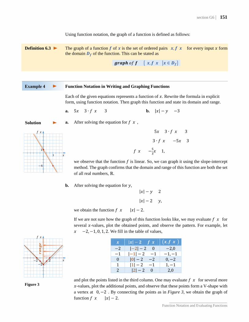
section G6 | 151


Using function notation, the graph of a function is defined as follows:

Definition 6.3 The graph of a function 𝒇𝒇 of 𝑨𝑨 is the set of ordered pairs (𝑨𝑨,𝒇𝒇(𝑨𝑨)) for every input 𝑥𝑥 form the domain 𝑫𝑫𝒇𝒇 of the function. This can be stated as

𝒓𝒓𝒓𝒓𝒓𝒓𝒈𝒈𝒉𝒉 𝑝𝑝𝑓𝑓 𝒇𝒇 = �(𝑨𝑨,𝒇𝒇(𝑨𝑨))�𝑨𝑨 ∈ 𝑫𝑫𝒇𝒇�

Function Notation in Writing and Graphing Functions Each of the given equations represents a function of 𝑥𝑥. Rewrite the formula in explicit

form, using function notation. Then graph this function and state its domain and range.

a. 5𝑥𝑥 + 3 ∙ 𝑓𝑓(𝑥𝑥) = 3 b. |𝑥𝑥| − 𝑦𝑦 = −3

a. After solving the equation for 𝑓𝑓(𝑥𝑥),

5𝑥𝑥 + 3 ∙ 𝑓𝑓(𝑥𝑥) = 3

3 ∙ 𝑓𝑓(𝑥𝑥) = −5𝑥𝑥 + 3

𝑓𝑓(𝑥𝑥) = −53𝑥𝑥 + 1,

we observe that the function 𝑓𝑓 is linear. So, we can graph it using the slope-intercept method. The graph confirms that the domain and range of this function are both the set of all real numbers, ℝ.

b. After solving the equation for 𝑦𝑦,

|𝑥𝑥| − 𝑦𝑦 = 2

|𝑥𝑥| − 2 = 𝑦𝑦,

we obtain the function 𝑓𝑓(𝑥𝑥) = |𝑥𝑥| − 2.

If we are not sure how the graph of this function looks like, we may evaluate 𝑓𝑓(𝑥𝑥) for several 𝑥𝑥-values, plot the obtained points, and observe the pattern. For example, let 𝑥𝑥 = −2,−1, 0, 1, 2. We fill in the table of values,

and plot the points listed in the third column. One may evaluate 𝑓𝑓(𝑥𝑥) for several more 𝑥𝑥-values, plot the additional points, and observe that these points form a V-shape with a vertex at (0,−2). By connecting the points as in Figure 3, we obtain the graph of function 𝑓𝑓(𝑥𝑥) = |𝑥𝑥| − 2.

𝑨𝑨 |𝑨𝑨| − 𝟐𝟐 = 𝒇𝒇(𝑨𝑨) �𝑨𝑨,𝒇𝒇(𝑨𝑨)� −2 |−2|− 2 = 0 (−2,0) −1 |−1| − 2 = −1 (−1,−1) 0 |0| − 2 = −2 (0,−2) 1 |1| − 2 = −1 (1,−1) 2 |2| − 2 = 0 (2,0)

Solution

𝑓𝑓(𝑥𝑥)

𝑥𝑥

1

−4

3

𝑓𝑓(𝑥𝑥)

𝑥𝑥 −2 −2

2


𝒓𝒓

Figure 3

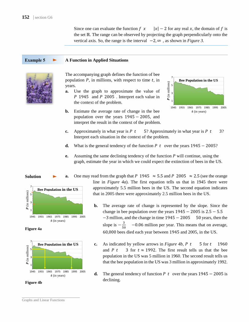
152 | section G6


Since one can evaluate the function 𝑓𝑓(𝑥𝑥) = |𝑥𝑥| − 2 for any real 𝑥𝑥, the domain of 𝑓𝑓 is the set ℝ. The range can be observed by projecting the graph perpendicularly onto the vertical axis. So, the range is the interval [−2,∞), as shown in Figure 3.

A Function in Applied Situations

The accompanying graph defines the function of bee population 𝑃𝑃, in millions, with respect to time 𝑡𝑡, in years. a. Use the graph to approximate the value of

𝑃𝑃(1945) and 𝑃𝑃(2005). Interpret each value in the context of the problem.

b. Estimate the average rate of change in the bee population over the years 1945 − 2005, and interpret the result in the context of the problem.

c. Approximately in what year is 𝑃𝑃(𝑡𝑡) = 5? Approximately in what year is 𝑃𝑃(𝑡𝑡) = 3? Interpret each situation in the context of the problem.

d. What is the general tendency of the function 𝑃𝑃(𝑡𝑡) over the years 1945 − 2005? e. Assuming the same declining tendency of the function 𝑃𝑃 will continue, using the

graph, estimate the year in which we could expect the extinction of bees in the US.

a. One may read from the graph that 𝑃𝑃(1945) ≈ 5.5 and 𝑃𝑃(2005) ≈ 2.5 (see the orange line in Figure 4a). The first equation tells us that in 1945 there were approximately 5.5 million bees in the US. The second equation indicates that in 2005 there were approximately 2.5 million bees in the US. b. The average rate of change is represented by the slope. Since the

change in bee population over the years 1945− 2005 is 2.5 − 5.5 =−3 million, and the change in time 1945 − 2005 = 50 years, then the slope is − 3

50= −0.06 million per year. This means that on average,

60,000 bees died each year between 1945 and 2005, in the US. c. As indicated by yellow arrows in Figure 4b, 𝑃𝑃(𝑡𝑡) = 5 for 𝑡𝑡 = 1960

and 𝑃𝑃(𝑡𝑡) = 3 for 𝑡𝑡 ≈ 1992. The first result tells us that the bee population in the US was 5 million in 1960. The second result tells us that the bee population in the US was 3 million in approximately 1992.

d. The general tendency of function 𝑃𝑃(𝑡𝑡) over the years 1945− 2005 is

declining.

Solution

Figure 4a

Figure 4b

𝑷𝑷 (i

n m

illio

ns)

1945 1955 1965 1975 1985 1995 2005 𝒕𝒕 (in years)

Bee Population in the US 7 5 3 1

𝑷𝑷 (i

n m

illio

ns)

1945 1955 1965 1975 1985 1995 2005 𝒕𝒕 (in years)


𝑷𝑷 (i

n m

illio

ns)

1945 1955 1965 1975 1985 1995 2005 𝒕𝒕 (in years)


section G6 | 153


e. Assuming the same declining tendency, to estimate the year in which the bee population in the US will disappear, we extend the 𝑡𝑡-axis and the approximate line of tendency (see the purple line in Figure 4c) to see where they intersect. After extending of the scale on the 𝑡𝑡-axis, we predict that the bee population will disappear around the year 2040.

Constructing Functions

Consider a circle with area 𝐴𝐴, circumference 𝐶𝐶, radius 𝑟𝑟, and diameter 𝑑𝑑.

a. Write 𝐴𝐴 as a function of 𝑟𝑟. b. Write 𝑟𝑟 as a function of 𝐴𝐴. c. Write 𝑑𝑑 as a function of 𝐶𝐶. d. Write 𝑑𝑑 as a function of 𝐴𝐴.

a. Using the formula for the area of a circle, 𝐴𝐴 = 𝜋𝜋𝑟𝑟2, the function 𝐴𝐴 of 𝑟𝑟 is 𝑨𝑨(𝒓𝒓) = 𝝅𝝅𝒓𝒓𝟐𝟐.

b. To express 𝑟𝑟 as a function of 𝐴𝐴, we solve the area formula for 𝑟𝑟.

𝐴𝐴 = 𝜋𝜋𝑟𝑟2 𝐴𝐴𝜋𝜋

= 𝑟𝑟2

�𝐴𝐴𝜋𝜋

= 𝑟𝑟

So, the function 𝑟𝑟 of 𝐴𝐴 is 𝒓𝒓(𝑨𝑨) = �𝑨𝑨𝝅𝝅

.

c. To write 𝑑𝑑 as a function of 𝐶𝐶, we start by connecting the formula for the circumference 𝐶𝐶 in terms of 𝑟𝑟 and the formula that expresses 𝑑𝑑 in terms of 𝑟𝑟. Since

𝐶𝐶 = 2𝜋𝜋𝑟𝑟 and 𝑑𝑑 = 2𝑟𝑟, then after letting 𝑟𝑟 = 𝑑𝑑

2 in the first equation, we obtain

𝐶𝐶 = 2𝜋𝜋𝑟𝑟 = 2𝜋𝜋 ∙𝑑𝑑2

= 𝜋𝜋𝑑𝑑,

which after solving for 𝑑𝑑, gives us 𝑑𝑑 = 𝐶𝐶𝜋𝜋. Hence, our function 𝑑𝑑 of 𝐶𝐶 is 𝒅𝒅(𝑪𝑪) = 𝑪𝑪

𝝅𝝅.

d. Since 𝑑𝑑 = 2𝑟𝑟 and 𝑟𝑟 = �𝐴𝐴𝜋𝜋 (as developed in the solution to Example 6b),

then 𝑑𝑑 = 2�𝐴𝐴𝜋𝜋. Thus, the function 𝑑𝑑 of 𝐴𝐴 is 𝒅𝒅(𝑨𝑨) = 𝟐𝟐�𝑨𝑨

𝝅𝝅.

Solution

𝑑𝑑

𝐶𝐶

𝑟𝑟 𝐴𝐴

Figure 4c

𝑷𝑷 (i

n m

illio

ns)

1945 1955 1965 1975 1985 1995 2005 2035 𝒕𝒕 (in years)


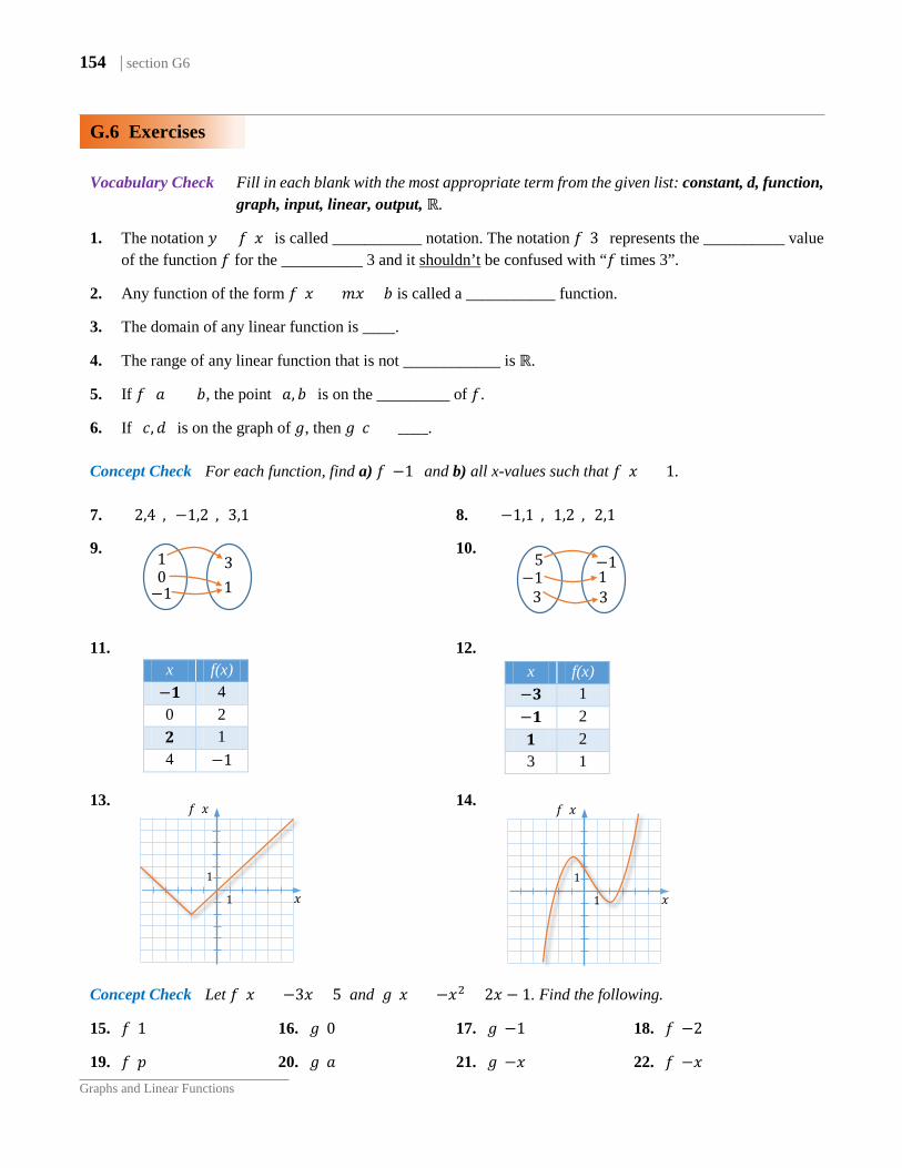
154 | section G6


G.6 Exercises

Vocabulary Check Fill in each blank with the most appropriate term from the given list: constant, d, function,

graph, input, linear, output, ℝ.

1. The notation 𝑦𝑦 = 𝑓𝑓(𝑥𝑥) is called ___________ notation. The notation 𝑓𝑓(3) represents the __________ value of the function 𝑓𝑓 for the __________ 3 and it shouldn’t be confused with “𝑓𝑓 times 3”.

2. Any function of the form 𝑓𝑓(𝑥𝑥) = 𝑚𝑚𝑥𝑥 + 𝑏𝑏 is called a ___________ function.

3. The domain of any linear function is ____.

4. The range of any linear function that is not ____________ is ℝ.

5. If 𝑓𝑓 (𝑎𝑎) = 𝑏𝑏, the point (𝑎𝑎, 𝑏𝑏) is on the _________ of 𝑓𝑓.

6. If (𝑐𝑐,𝑑𝑑) is on the graph of 𝑟𝑟, then 𝑟𝑟(𝑐𝑐) = _____. Concept Check For each function, find a) 𝑓𝑓(−1) and b) all x-values such that 𝑓𝑓(𝑥𝑥) = 1. 7. {(2,4), (−1,2), (3,1)} 8. {(−1,1), (1,2), (2,1)}

9. 10.

11. 12.

13. 14.

Concept Check Let 𝑓𝑓(𝑥𝑥) = −3𝑥𝑥 + 5 and 𝑟𝑟(𝑥𝑥) = −𝑥𝑥2 + 2𝑥𝑥 − 1. Find the following.

15. 𝑓𝑓(1) 16. 𝑟𝑟(0) 17. 𝑟𝑟(−1) 18. 𝑓𝑓(−2)

19. 𝑓𝑓(𝑝𝑝) 20. 𝑟𝑟(𝑎𝑎) 21. 𝑟𝑟(−𝑥𝑥) 22. 𝑓𝑓(−𝑥𝑥)

x f(x) −𝟏𝟏 4 0 2 𝟐𝟐 1 4 −1

x f(x) −𝟑𝟑 1 −𝟏𝟏 2 𝟏𝟏 2 3 1

−1 5

3

−1 1

3 0 1 3

1 −1

𝑓𝑓(𝑥𝑥)

𝑥𝑥

1

1

𝑓𝑓(𝑥𝑥)

𝑥𝑥

1

1

section G6 | 155


23. 𝑓𝑓(𝑎𝑎 + 1) 24. 𝑟𝑟(𝑎𝑎 + 2) 25. 𝑟𝑟(𝑥𝑥 − 1) 26. 𝑓𝑓(𝑥𝑥 − 2)

27. 𝑓𝑓(2 + ℎ) 28. 𝑟𝑟(1 + ℎ) 29. 𝑟𝑟(𝑎𝑎 + ℎ) 30. 𝑓𝑓(𝑎𝑎 + ℎ)

31. 𝑓𝑓(3) − 𝑟𝑟(3) 32. 𝑟𝑟(𝑎𝑎) − 𝑓𝑓(𝑎𝑎) 33. 3𝑟𝑟(𝑥𝑥) + 𝑓𝑓(𝑥𝑥) 34. 𝑓𝑓(𝑥𝑥 + ℎ) − 𝑓𝑓(𝑥𝑥)

Concept Check Fill in each blank with the correct response.

35. The graph of the equation 2𝑥𝑥 + 𝑦𝑦 = 4 is a ___________. One point that lies on this graph is (3, ____). If we solve the equation for 𝑦𝑦 and use function notation, we obtain 𝑓𝑓(𝑥𝑥) = ______________ . For this function, 𝑓𝑓(3) = _______ , meaning that the point (____ , ____) lies on the graph of the function.

Graph each function. Give the domain and range.

36. 𝑓𝑓(𝑥𝑥) = −2𝑥𝑥 + 5 37. 𝑟𝑟(𝑥𝑥) = 13𝑥𝑥 + 2 38. ℎ(𝑥𝑥) = −3𝑥𝑥

39. 𝐹𝐹(𝑥𝑥) = 𝑥𝑥 40. 𝐺𝐺(𝑥𝑥) = 0 41. 𝐻𝐻(𝑥𝑥) = 2

42. 𝑥𝑥 − ℎ(𝑥𝑥) = 4 43. −3𝑥𝑥 + 𝑓𝑓(𝑥𝑥) = −5 44. 2 ∙ 𝑟𝑟(𝑥𝑥) − 2 = 𝑥𝑥

45. 𝑘𝑘(𝑥𝑥) = |𝑥𝑥 − 3| 46. 𝑚𝑚(𝑥𝑥) = 3 − |𝑥𝑥| 47. 𝑞𝑞(𝑥𝑥) = 𝑥𝑥2

48. 𝑄𝑄(𝑥𝑥) = 𝑥𝑥2 − 2𝑥𝑥 49. 𝑝𝑝(𝑥𝑥) = 𝑥𝑥3 + 1 50. 𝑡𝑡(𝑥𝑥) = √𝑥𝑥 Solve each problem.

51. A taxicab driver charges $1.75 per kilometer.

a. Fill in the table with the correct charge 𝑓𝑓(𝑥𝑥) for a trip of 𝑥𝑥 kilometers. b. Find the linear function that gives the amount charged 𝑓𝑓(𝑥𝑥) = ___________. c. Graph 𝑓𝑓(𝑥𝑥) for the domain {0, 1, 2, 3}. 52. The table represents a linear function.

a. What is 𝑓𝑓(3)? b. If 𝑓𝑓(𝑥𝑥) = −2.5, what is the value of 𝑥𝑥? c. What is the slope of this line? d. What is the 𝑦𝑦-intercept of this line? e. Using your answers to parts c. and d., write an equation for 𝑓𝑓(𝑥𝑥). 53. A car rental is $150 plus $0.20 per kilometer. Let 𝑥𝑥 represent the number of kilometers driven and 𝑓𝑓(𝑥𝑥)

represent the total cost to rent the car.

a. Write a linear function that models this situation. b. Find 𝑓𝑓(250) and interpret your answer in the context of this problem. c. Find the value of 𝑥𝑥 satisfying the equation 𝑓𝑓(𝑥𝑥) = 230 and interpret it in the context of this problem. 54. A window cleaner charges $50 per visit plus $35 per hour.

a. Express the total charge, 𝐶𝐶, as a function of the number of hours worked, 𝑝𝑝.

x f(x) 𝟎𝟎 1 𝟐𝟐 3

x f(x) 𝟎𝟎 3.5 1 2.3 𝟐𝟐 1.1 3 −0.1 4 −1.3 5 −2.5

156 | section G6


b. Find 𝐶𝐶(4) and interpret your answer in the context of this problem. c. If the window cleaner charged $295 for his job, what was the number of hours for which he has charged?

55. Refer to the accompanying graph to answer the questions below. a. What numbers are possible values of the independent variable? The

dependent variable? b. For how long is the water level increasing? Decreasing? c. How many gallons of water are in the pool after 90 hr? d. Call this function 𝑓𝑓. What is 𝑓𝑓(0)? What does it mean? e. What is 𝑓𝑓(25)? What does it mean? Analytic Skills

The graph represents the distance that a person is from home while walking on a straight path. The t-axis represents time, and the d-axis represents distance. Interpret the graph by describing the person’s movement.

56. 57.

58. Consider a square with area 𝐴𝐴, side 𝑡𝑡, perimeter 𝑃𝑃, and diagonal 𝑑𝑑. (Hint for question 58 c and d: apply the Pythagorean equation 𝑎𝑎2 + 𝑏𝑏2 = 𝑐𝑐2, where 𝑐𝑐 is the hypotenuse of a right angle triangle with arms 𝑎𝑎 and 𝑏𝑏.)

a. Write 𝐴𝐴 as a function of 𝑡𝑡. b. Write 𝑡𝑡 as a function of 𝑃𝑃. c. Write 𝑑𝑑 as a function of 𝑡𝑡. d. Write 𝑑𝑑 as a function of 𝑃𝑃.

hours

2000

3000

0 100

𝑓𝑓(𝑡𝑡)

𝑡𝑡

1000

75

4000

0

gallo

ns

50 25

Gallons of Water in a Pool at Time 𝒕𝒕

𝑑𝑑

𝑡𝑡

𝑑𝑑

𝑡𝑡

𝒔𝒔

𝒔𝒔

𝒅𝒅

Graphs and Linear Functions - Anna Kuczynska · Graphs and Linear Functions . Graphs of Linear...

Documents

Transcript of Graphs and Linear Functions - Anna Kuczynska · Graphs and Linear Functions . Graphs of Linear...