Graph Theory lecture notes

1 Definitions and examples

1–1 Definitions

Definition 1.1. A graph is a set of points, called vertices, together with a collection of lines,called edges, connecting some of the points. The set of vertices must not be empty.

If G is a graph we may write V (G) and E(G) for the set of vertices and the set of edgesrespectively. The number of vertices (sometimes called the “order” of G) is written |G|, andthe number of edges (sometimes called the “size” of G) is written e(G).

A graph may have multiple edges, i.e. more than one edge between some pair of vertices,or loops, i.e. edges from a vertex to itself. A graph without multiple edges or loops is calledsimple. Many natural problems only make sense in the setting of simple graphs.

If two vertices are joined by an edge they are called adjacent.

Definition 1.2. For each vertex v, the set of vertices which are adjacent to v is called theneighbourhood of v, and written Γ(v). A neighbour of v is any element of the neighbourhood.

Remark. Normally we do not include v in Γ(v); it is only included if there is a loop.

Definition 1.3. The degree of a vertex v, written d(v), is the number of ends of edges whichconnect to that vertex.

In other words if we wrote down as a list the corresponding pair of vertices for every edge,the degree of a vertex is the number of times it appears in that list. As both ends of a loop goto the same vertex, each loop contributes 2 to the degree. In a simple graph, d(v) = |Γ(v)|.

What happens if we add up the degrees of all the vertices?

Lemma 1.4 (Euler’s handshaking lemma). The sum of the degrees of the vertices of a graphis equal to twice the number of edges.

We may write the sum of the degrees in two equivalent forms. Let d1, d2, . . . be the degreesof vertices in G and ni be the number of vertices with degree i. Then d1 + d2 + d3 + · · · =n1 + 2n2 + 3n3 + · · · ; the handshaking lemma tells us that each is equal to twice the number ofedges. In particular, both sums are even.

In order for two graphs to be the same, they must have the same set of vertices and thesame set of edges. This is very restrictive, and normally all we are interested in is whether theyare essentially the same, that is to say they are different labellings of the same basic structure.What follows is a formal definition of this idea.

Definition 1.5. If G and H are two graphs then an isomorphism between G and H is abijection φ : V (G)→ V (H) such that for any v, w ∈ V (G) the number of edges between v andw in G is the same as the number of edges between φ(v) and φ(w) in H. If such a bijectionexists we say that G and H are isomorphic and write G ∼= H.

Example 1.6. Give a bijection which shows that the graphs below are isomorphic.

1

Definition 1.7. Let G and H be graphs. We say that H is a subgraph of G (or G “contains”H) if V (H) ⊆ V (G) and E(H) ⊆ E(G). If V (H) = V (G) and E(H) ⊆ E(G) then H is aspanning subgraph.

G is always a subgraph of itself. A proper subgraph of G is any subgraph other than Gitself.

One type of subgraph of particular importance is an induced subgraph: H is an inducedsubgraph of G if V (H) ⊆ V (G) and E(H) is the set of edges in E(G) with both vertices inV (H).

1–2 Examples and types of graphs

1. Empty graphs. En has n vertices and no edges.

2. Complete graphs. Kn has n vertices and each vertex is connected to each other vertex byprecisely one edge.

3. Paths and cycles. The path Pn is the graph with n vertices v1, v2, . . . vn and n− 1 edgesv1v2, v2v3, . . . vn−1vn. The cycle Cn is graph with n edges obtained from Pn by adding anedge between the two ends; it is the graph of a polygon with n sides. The wheel graphWn+1 is the graph obtained from Cn by adding another vertex and edges from it to allthe others.

4. Platonic graphs. There are five platonic graphs corresponding to the five platonic solids.See the additional sheet for full details. We can define graphs similarly for other polyhedra;there are 13 graphs which correspond to archimedean solids, for example.

5. Disjoint union of graphs. From any two graphs G1 and G2 we can form the disjoint unionG1 tG2 which consists of separate copies of G1 and G2, with no edges between them.

Definition 1.8. A graph is connected if it cannot be written as a disjoint union of twographs.

6. Regular graphs. A regular graph is one in which all the vertices have the same degree.

Definition 1.9. G is k-regular if every vertex has degree k.

“Cubic” is another word for 3-regular.

7. Bipartite graphs.

Definition 1.10. A graph is bipartite if we can colour the vertices red and blue in sucha way that each edge connects a red vertex to a blue vertex.

2

The complete bipartite graph Km,n has m red vertices and n blue vertices, and fromevery red vertex there is exactly one edge to every blue vertex.

8. The complement. Let G be a simple graph. The complement of G, written G or G,is the simple graph with the same vertex set as G such that two vertices are adjacent inG if and only if they are not adjacent in G. The complement of the complement is theoriginal graph, i.e. (G) = G.

Examples of complements relating graphs we have already seen are Kn = En and Ks,t =Ks tKt.

2 Connectivity and Trees

2–1 Connectivity

Recall that a graph is disconnected if it is the disjoint union of two other graphs, and connectedotherwise. We will find it convenient to think of connectivity in terms of being able to get fromany vertex to any other.

Definition 2.1. A walk in a graph is a sequence of the form v1, e1, v2, e2 . . . vr, for some r > 1,where the vi are vertices and ei is an edge from vi to vi+1 for each 1 6 i < r.

Remark. If r = 1 the walk consists of a single vertex and no edges; this is still valid.

Definition 2.2. A trail is a walk in which no edge appears more than once.

Definition 2.3. A path is a walk in which no vertex appears more than once.

We might want to know whether there is a path (or trail, or walk) between specific verticesx and y. First we note that the answer is the same in each case.

Lemma 2.4. The following are equivalent:

1. there is a path from x to y;

2. there is a trail from x to y;

3. there is a walk from x to y.

Proof. First note that, since any path is also a trail and any trail is also a walk, 1)⇒ 2)⇒ 3).So it suffices to prove that 3)⇒ 1). We will complete the proof in lectures.

Write x 99K y if there is a path from x to y; recall that the single vertex x is a path of length0 so x 99K x. The relation 99K is an equivalence relation, since if x 99K y and y 99K z thenwe can put the two paths together to get a walk from x to z, and by Lemma 2.4 this impliesx 99K z. Consequently we may partition the vertices into equivalence classes of 99K, and we callthese the components of G.

Theorem 2.5. A graph G is connected if and only if there is a path between every pair ofvertices.

Proof (non-examinable). Write V for the set of vertices. Suppose there is no path from v to w,for v, w ∈ V . Let C be the component containing v. Certainly v ∈ C and w ∈ V \ C, so bothsets are non-empty. There are no edges between C and V \ C, since there is no path from anyvertex in C to any vertex not in C, by definition. So, writing G1 for the subgraph induced byC and G2 for the subgraph induced by V \ C, G = G1 tG2.

3

Conversely, suppose G = G3 t G4 is not connected. Let v be a vertex of G3 and w be avertex of G4. If there is a path in G from v to w then let x be the last vertex on the path whichbelongs to G3, and y be the next vertex (which exists since x 6= w). Then xy is not an edge ofG3, since y is not in G3, nor is it an edge of G4, since x is not in G4. But xy is an edge of G,so G 6= G3 tG4.

We may therefore equivalently define a connected graph to be one which has a path betweenevery pair of vertices; we will generally find this definition easier to work with.

2–2 Trees

We say a graph has a cycle if it has a subgraph isomorphic to Cn for some n.

Definition 2.6. A tree is a connected graph with no cycles. A forest is a graph with nocycles.

Remark. A tree must be a simple graph.

Drawing some trees suggests that they all have the same number of edges. We’ll prove thisin two stages.

Theorem 2.7. A connected graph with n vertices has at least n− 1 edges.

Proof. We use induction on the number of vertices. When n = 1 there is nothing to prove. Weassume the theorem is true for n = k − 1 and show that this implies it is also true for n = k.We will complete the proof in lectures.

Theorem 2.8. Let G be a connected graph with n vertices. Then G is a tree if and only ife(G) = n− 1.

Proof. We have two things to prove: “if” and “only if”. For the first, it is sufficient to showthat if G is not a tree, so G has a cycle, then it has more than n− 1 edges. For the second, weshow by induction on n that any tree with n vertices has n− 1 edges. We will complete this inlectures.

If G is a tree, we refer to a vertex of G with degree 1 as a leaf.

Example 2.9. Show that any tree with at least two vertices has at least two leaves.

Let G be a connected graph on n vertices. A spanning tree for G is a subgraph which isa tree containing all vertices of G. Such a subgraph must exist.

We can define a simple algorithm to identify a spanning tree:

1. if there are only n− 1 edges remaining then we have found a tree, so stop;

2. the graph is connected and not a tree, so find a cycle;

3. delete any edge from this cycle;

4. go to step 1.

The spanning tree found is not unique because of the choice we have in step 3. If G is a graphand T a specified spanning tree then we call the edges of T branches and the remaining edgesof G chords. Each chord lies in a cycle whose other edges are branches; this cycle is unique.These cycles (one for each chord) are called the fundamental cycles of T .

4

3 Applications of trees

3–1 Kruskal’s algorithm

Definition 3.1. A weighted graph is a graph where each edge has a positive number (or“weight”) associated with it.

The weights typically represent distance, time or cost of travel between vertices. The weightof a subgraph is the sum of the weights of all the edges which are included.

Kruskal’s algorithm finds a minimum-weight spanning tree in a weighted graph. A typicalapplication is that we have several towns which we wish to connect up by adding water pipesbetween pairs of towns, minimising the total length of pipe used; we have a table of distancesbetween pairs of towns. Since any connected graph which is not a tree will contain a spanningtree which uses less pipe, the answer will always be a tree. So we are looking for a spanning treewith the minimum possible total edge length. This need not be unique; there may be severaldifferent spanning trees but with the same total edge length. Our table of distances might be

A3 B5 2 C1 4 9 D12 13 9 2 E10 7 6 9 6 F

The algorithm to find a minimal spanning tree is based on the following observation.

Lemma 3.2. Suppose the edge between A and B is at least as short as every other edge. Thenthere exists a minimal spanning tree which includes the edge AB.

We will prove this in lectures

Our algorithm is therefore:

1. list the edges in increasing order of length;

2. consider the smallest remaining edge;

3. if we can add that edge to T without creating a cycle, do so, otherwise discard it;

4. if we have n− 1 edges, T is a spanning tree so stop;

5. otherwise go back to step 2.

Example 3.3. Carry out this algorithm for the distances given above.

Note that this assumes that the only permitted vertices are the towns specified. In a real-world scenario we might be able to do better. For example, suppose towns A, B and C arearranged in an equilateral triangle of side length 10 miles. The minimal spanning tree haslength 20 miles, but we can do better by placing a pumping station somewhere in the middleand connecting it to each town. What is the minimum length of pipe needed if we do this?

5

3–2 Chemistry

Alkanes have chemical formula CnH2n+2. The first four (n = 1, . . . 4) are methane, ethane,propane and butane, shown below.

H H H

H C H H C C H

H H H

H H H H H H H

H C C C H H C C C C H

H H H H H H H

However, there is another compound, isobutane, which also has the formula C4H10.

H H H

H C C C H

H C H

H H H

Butane and isobutane are called structural isomers; they have the same formula but theatoms are connected in a different way. The number of isomers increases rapidly; C25H52 hasover one million isomers.

We can relate the isomers of CnH2n+2 to graphs. Because of the physical properties of theatoms, each carbon atom must be bonded to 4 other atoms (chemists say carbon has “valency”4) and each hydrogen atom to 1 other atom, and the whole molecule must be connected.So we have a connected graph with n vertices of degree 4 and 2n + 2 vertices of degree 1, so2e = 4n+(2n+2) and so e = 3n+1, which is one less than the number of vertices. Consequentlythe graph is a tree.

All the hydrogen atoms are leaves; if we remove them the remaining carbon vertices mustform a smaller tree. So if we want to know how many isomers there are, we need to count thenumber of non-isomorphic trees on n vertices, with no vertex having degree higher than 4.

Example 3.4. How many isomers of pentane (C5H12) are there?

Exercise 3.5. How many isomers of hexane (C6H14) are there?

We might also consider compounds which have some other atoms. Chlorine (Cl) has valency1, oxygen (O) has valency 2, and nitrogen (N) has valency 3. We can again work out if thegraph is a tree, and draw the trees with the appropriate number of vertices, but a tree willtypically give more than one isomer since we will need to decide which vertex is the nitrogenatom, say.

Example 3.6. Does C3H8O form a tree? How many isomers does it have?

3–3 Bracings

See the first homework sheet.

6

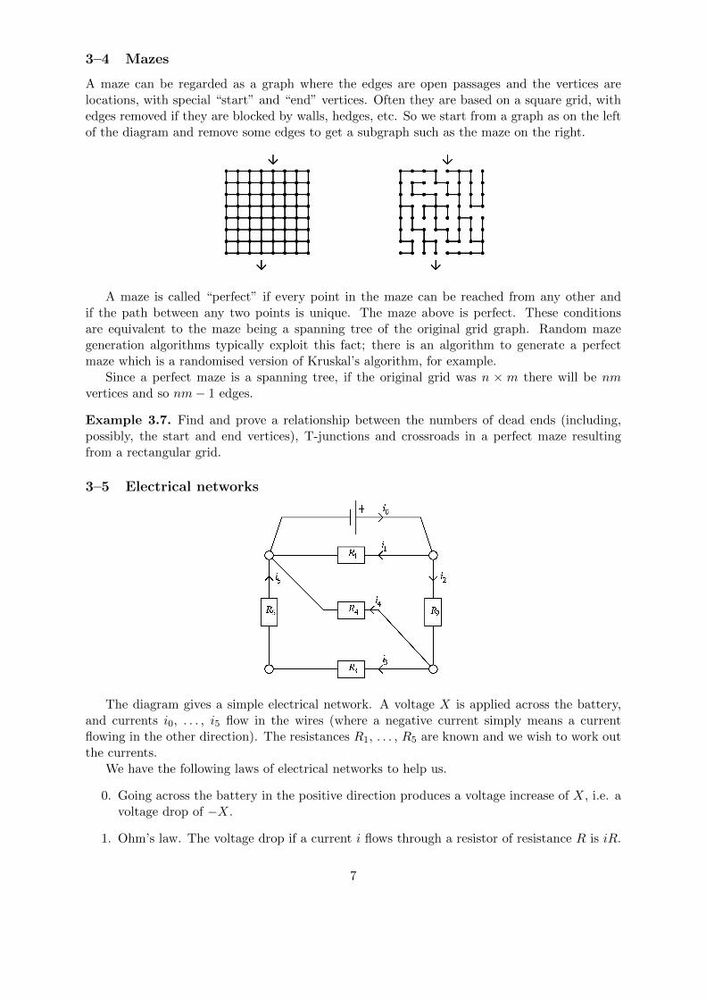
3–4 Mazes

A maze can be regarded as a graph where the edges are open passages and the vertices arelocations, with special “start” and “end” vertices. Often they are based on a square grid, withedges removed if they are blocked by walls, hedges, etc. So we start from a graph as on the leftof the diagram and remove some edges to get a subgraph such as the maze on the right.

A maze is called “perfect” if every point in the maze can be reached from any other andif the path between any two points is unique. The maze above is perfect. These conditionsare equivalent to the maze being a spanning tree of the original grid graph. Random mazegeneration algorithms typically exploit this fact; there is an algorithm to generate a perfectmaze which is a randomised version of Kruskal’s algorithm, for example.

Since a perfect maze is a spanning tree, if the original grid was n × m there will be nmvertices and so nm− 1 edges.

Example 3.7. Find and prove a relationship between the numbers of dead ends (including,possibly, the start and end vertices), T-junctions and crossroads in a perfect maze resultingfrom a rectangular grid.

3–5 Electrical networks

The diagram gives a simple electrical network. A voltage X is applied across the battery,and currents i0, . . . , i5 flow in the wires (where a negative current simply means a currentflowing in the other direction). The resistances R1, . . . , R5 are known and we wish to work outthe currents.

We have the following laws of electrical networks to help us.

0. Going across the battery in the positive direction produces a voltage increase of X, i.e. avoltage drop of −X.

1. Ohm’s law. The voltage drop if a current i flows through a resistor of resistance R is iR.

7

2. Kirchoff’s first law. The sum of currents entering a node is equal to the sum of currentsleaving it. This gives us four equations. However, these equations are not linearly inde-pendent and any one of them may be deduced from the other three. So we have threeequations (in six unknowns).

3. Kirchoff’s second law. The sum of voltage drops around any cycle is 0. Together withOhm’s law this gives us several additional equations – one for each cycle.

To avoid redundancy in Kirchoff’s second law we should take a system of fundamental cycles;this will produce linearly independent equations. Any spanning tree will have three fundamentalcycles, so gives us three more equations for a total of six linearly independent equations in sixunknowns. These will have a unique solution. In general if there are n vertices and e edgeswe have n − 1 equations from the first law and e − (n − 1) fundamental cycles, so a total of eequations.

Example 3.8. Pick a spanning tree and write down six linearly independent equations for thecircuit shown. Solve them when X = 240 V, R1 = R2 = R3 = R4 = 20 Ω and R5 = 30 Ω.

4 Eulerian graphs

4–1 Euler trails

Is it possible to draw the graph shown without lifting thepen from the paper, or going over the same line twice?

Recall that a walk is a route round the edges and vertices of a graph, and a trail is a walk inwhich the edges used are distinct. A trail (or walk) is closed if it starts and ends at the samevertex. A closed trail is not necessarily a cycle, since it may visit the same vertex several times.

Definition 4.1. A graph is Eulerian if it has a closed trail which includes every edge. A graphis semi-Eulerian if has a trail which is not closed but which includes every edge.

We refer to a closed trail which includes every edge as an Euler trail. Euler observed that,provided the graph is connected, we can tell whether it is Eulerian, semi-Eulerian, or neitherjust by looking at the degrees of the vertices. It is easy to see that an Eulerian graph must haveall its degrees even, but harder to show that a connected graph which satisfies this property isindeed Eulerian.

Lemma 4.2. If G is a graph with all vertices having even degree, then the edges of G may bepartitioned into disjoint cycles.

We will prove this in lectures

Next we show that for a connected graph we can stitch together these cycles into an Euler trail.

Theorem 4.3 (Euler). A connected graph G is Eulerian if and only if every vertex has evendegree.

8

We will prove this in lectures

We get an equivalent condition for semi-Eulerian graphs by observing that a graph is semi-Eulerian if and only if we make it Eulerian by adding a single edge.

Theorem 4.4 (Euler). A connected graph G is semi-Eulerian if and only if exactly two verticeshave odd degree.

We will prove this in lectures

Fleury’s algorithm finds an Euler trail in an Eulerian graph, or a trail which uses every edge ina semi-Eulerian graph.

Definition 4.5. A bridge in a connected graph is an edge whose removal will disconnectthe graph. In an unconnected graph, a bridge is an edge whose removal will disconnect thecomponent it is in.

Fleury’s algorithm proceeds as follows. If the graph is Eulerian, start at any vertex andmove along any edge, deleting that edge once you have crossed it, but only crossing a bridgeif there is no alternative. If it is semi-Eulerian, start at either vertex of odd degree and thenapply the same algorithm.

4–2 The Chinese Postman problem

A postman delivers letters to a set of streets which form the edges of a connected graph G; thevertices of G are junctions between streets. He knows the length of each street (different streetsmay have different lengths). He needs to start and finish at the same junction, and travel alonga walk which covers every street at least once. What is the shortest walk he can take whichachieves this?

The problem was originally studied by Mei-Ko Kwan (1962), who gave a necessary andsufficient condition for a shortest route. Edmonds and Johnson subsequently (1973) gave anefficient algorithm for finding the optimal closed walk.

The postman can certainly do no better than the total length L of all the streets, and aroute of this length is precisely an Euler trail so he can do this if and only if G is Eulerian. Ifit is not Eulerian he will need to travel along some streets more than once.

Theorem 4.6. If the graph is semi-Eulerian, x and y are the two vertices of odd degree, andthe shortest path between x and y has length P then the shortest postman route has lengthL+ P .

Proof. The postman can certainly achieve this, by walking along a trail from x to y which coversevery edge and then back to x along a shortest path.

To show that he can do no better, it is sufficient to show that in any closed walk whichcovers every edge, the set of edges covered twice include a path from x to y. We will completethe proof in lectures.

We shall see an efficient algorithm to find the shortest path in a later lecture. The generalcase, where G may have several vertices of odd degree, is much harder.

9

5 Hamilton cycles

Recall that a cycle in a given graph is a subgraph isomorphic to Cn for some n, and a path in agraph is a subgraph isomorphic to Pm for some m (or, equivalently, a walk in which no vertexappears more than once).

Definition 5.1. A Hamilton cycle in a graph is a cycle which includes every vertex, and aHamilton path is a path which includes every vertex.

Definition 5.2. A graph is Hamiltonian if it has a Hamilton cycle, and semi-Hamiltonianif it is not Hamiltonian but does have a Hamilton path.

In paths and cycles all the vertices have to be distinct (unlike trails where only edges have tobe distinct). So a Hamilton path or cycle visits every vertex exactly once; an Eulerian trail usesevery edge exactly once. It is much harder to determine whether a given graph is Hamiltonianthan whether it is Eulerian.

Some examples of Hamiltonian graphs are the complete graph Kn (for n > 3) and thecomplete bipartite graph Kn,n (for n > 2), all five platonic graphs, and (harder) the “knight’sgraph” whose vertices are the squares of a chessboard and whose edges connect pairs of verticeswhich are a knight’s move apart.

Exercise 5.3. Verify that the dodecahedron and icosahedron are Hamiltonian.

Some examples of graphs which are not Hamiltonian are the complete bipartite graph Kn,m

for n 6= m (since any cycle in a bipartite graph must alternate between red and blue vertices,so must have the same number of each) and any graph with a bridge (since once we cross thebridge we can’t get back).

There is no simple if-and-only-if condition for a graph to be Hamiltonian. There are somesufficient conditions, most of which say that a graph with plenty of edges everywhere is Hamil-tonian. The first of these was proved by G. A. Dirac (1952).

Theorem 5.4 (Dirac). If G is a simple graph with n > 3 vertices and minimum degree at leastn2 then G is Hamiltonian.

We will not give Dirac’s original proof, but instead deduce Dirac’s theorem from the subse-quent result proved by Ore (1960).

Theorem 5.5 (Ore). Let G be a simple graph with n > 3 vertices. Suppose that every pairof distinct non-adjacent vertices (u, v) satisfies the inequality d(u) + d(v) > n. Then G isHamiltonian.

Proof. Outline; we will fill in the details in lectures.

1. Suppose G is not Hamiltonian. We may assume G is semi-Hamiltonian (why?).

2. Take a Hamilton path v1 · · · vn, and imagine it running from left to right. Show that thereis some edge on the path whose right-hand vertex is adjacent to v1 and whose left-handvertex is adjacent to vn.

3. Show how we may form a Hamilton cycle given such an edge.

Example 5.6. What is the smallest number of edges that will ensure that a simple graph on10 vertices is Hamiltonian?

10

We can deduce Dirac’s theorem immediately from Ore’s theorem: if d(v) > n2 for every v

then d(u) + d(v) > n for every pair of vertices, so G is Hamiltonian. The n2 in Dirac’s theorem

is best possible.

Exercise 5.7. Any graph can be categorised as Eulerian (E), semi-Eulerian (SE), or neither(NE) and also as Hamiltonian (H), semi-Hamiltonian (SH), or neither (NH). Combining thesegives 9 categories of graphs; draw a simple connected example for each.

6 The Travelling Salesman problem

A travelling salesman needs to visit each of a group of cities, returning to his starting point. Thedistance from each city to each other is known, and he wishes to minimise his total distance.This corresponds to finding a Hamilton cycle of minimum weight in a weighted complete graph.This is a hard problem. There are (n − 1)! Hamilton cycles to choose from, and the factorialsgrow quite quickly. When n = 10 we have 9! = 362880; when n = 20 we have 19! ≈ 1017; andwhen n = 71 we have 70! ≈ 10100.

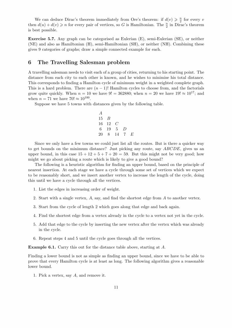
Suppose we have 5 towns with distances given by the following table.

A15 B16 12 C6 19 5 D20 8 14 7 E

Since we only have a few towns we could just list all the routes. But is there a quicker wayto get bounds on the minimum distance? Just picking any route, say ABCDE, gives us anupper bound, in this case 15 + 12 + 5 + 7 + 20 = 59. But this might not be very good; howmight we go about picking a route which is likely to give a good bound?

The following is a heuristic algorithm for finding an upper bound, based on the principle ofnearest insertion. At each stage we have a cycle through some set of vertices which we expectto be reasonably short, and we insert another vertex to increase the length of the cycle, doingthis until we have a cycle through all the vertices.

1. List the edges in increasing order of weight.

2. Start with a single vertex, A, say, and find the shortest edge from A to another vertex.

3. Start from the cycle of length 2 which goes along that edge and back again.

4. Find the shortest edge from a vertex already in the cycle to a vertex not yet in the cycle.

5. Add that edge to the cycle by inserting the new vertex after the vertex which was alreadyin the cycle.

6. Repeat steps 4 and 5 until the cycle goes through all the vertices.

Example 6.1. Carry this out for the distance table above, starting at A.

Finding a lower bound is not as simple as finding an upper bound, since we have to be able toprove that every Hamilton cycle is at least as long. The following algorithm gives a reasonablelower bound.

1. Pick a vertex, say A, and remove it.

11

2. Use Kruskal’s algorithm to find a minimum spanning tree for the remainder.

3. Find the two shortest edges from A to the rest of the graph.

4. Add these two lengths to the total length of the spanning tree to get a lower bound.

Lemma 6.2. This gives a lower bound on the travelling salesman problem.

We will prove this in lectures

Example 6.3. Find a lower bound for the distance table above, removing A.

In both cases the bound we get will depend on the choice of vertex we make at the start.

7 Directed graphs and directed Hamilton paths

A directed graph, or digraph, is like a graph, but instead of a set of edges between pairsof vertices we have a set of arcs, where each arc goes from one vertex to another (or back toitself). We draw arcs as arrows. We might think of these as a system of one-way streets. If wewanted to represent a 2-way street we would do this by having an arc from a to b and anotherarc from b to a.

A directed path in a directed graph is a sequence of arcs of the form v1 → v2, v2 → v3, . . . ,vk−1 → vk, where the vi are distinct vertices. In other words it corresponds to our previousnotion of a path but all the arcs must be going in the right direction. A directed cycle is likewisea sequence v1 → v2, v2 → v3, . . . , vk−1 → vk, vk → v1.

Consider the following puzzle. Points a to g are arranged around a circle clockwise. From a,d or f we are allowed to move exactly 3 spaces either clockwise or anticlockwise (so from a wecould go to d or e); from b or e we are allowed to move 2 spaces in either direction; and from cor g we are allowed to move one space in either direction. Can we move around following theserules and visit every point exactly once?

This is asking for a Hamilton path in a directed graph obtained by drawing arcs a → dand a → e, b → g and b → d, and so on. There is no efficient algorithm, but we might try tosystematically search for a solution either by breadth-first or depth-first searching.

7–1 Depth-first search

Choose a vertex to start from, a, say. Next choose any unvisited vertex reachable from a, andgo there. Keep going, at every stage choosing an unvisited vertex which we are allowed to moveto – mark any vertex from which we have only one option. Keep going until you either find aHamilton path or are stuck – when you are stuck backtrack to the previous vertex where therewas a choice and choose differently.

Example 7.1. Find a solution to the puzzle above using depth-first search.

7–2 Breadth-first search

We aim to build up a tree of possible routes. Start with a in the first column, then put thepossible vertices you can get to from a in the next column, then the possible ways to continuethese paths in the third column, and so on. We will find all possibilities this way.

Example 7.2. Find all solutions to the puzzle above using breadth-first search.

12

Exercise 7.3. Arrange points a to k in a circle clockwise. From g or j you may move one stepin either direction; from d or f exactly two steps in either direction; from b, e or h you maymove exactly three steps in either direction; from a, c or k, four; and from i, five. Find a routethrough all the vertices starting at a.

8 Shortest and longest paths

8–1 Shortest paths

Recall that a weighted graph (or digraph) is one where each edge (or arc) has a positive “weight”,which we typically think of as representing distance, time or cost of travel, associated with it. Itis natural to ask for the shortest (in terms of total weight) path between two points in a graphor digraph; we have already seen an application of this in the Chinese Postman problem. Howmight we go about finding the shortest path from A to L in the following weighted graph?

B2

4

D2

G6

J

5

A

3

8

2

E2

1

H

5

9

6

L

C9

6

F2

1

I2

K

3

Dijkstra’s algorithm finds the shortest distance to every vertex. We will not give a formalproof that it works. At each step of the algorithm there will be some vertices marked withdistances, and we need to distinguish which are final answers and which are merely bounds(which may change). We typically do this by circling the final answers.

1. Start by marking the start vertex as distance 0, and circle it.

2. For each vertex adjacent to the start vertex, we calculate a bound which is the length ofthe edge to that vertex.

3. Find the vertex with the smallest bound among vertices which do not have final answerscircled. Circle that bound, and mark the edge which gave that bound.

4. For each edge leaving the vertex you have just marked with a final answer, add that answerto the length of an edge to get a bound for the vertex that edge goes to. If it is smallerthan the current bound at that vertex, replace the old bound with this one.

5. Repeat steps 3 and 4 until all vertices have their exact distances marked.

Example 8.1. Carry out Dijkstra’s algorithm on the graph above.

The edges we’ve marked form a tree and the shortest path from A to any given vertex is thepath contained in that tree.

8–2 Minimum-cost maximum flows

We have a directed graph where the arcs represent pipes. Water flows along the pipes from Ato G. The circled numbers on the arcs are capacities; they represent how much water can flowthrough the given pipe.

13

B 3© //

3©%%

D

4©%%

A

4©99

4©%%

E 5© //

3©%%

G

C 4© //

4©99

F

4©99

We want to send as much water as possible through the network. In order to do this wechoose a path through the network, then put as much water as we can through that path. Sowe might start by putting 3 units along the path ABDG. This uses up all the capacity of BD,and AB and DG have 1 unit of capacity left. Then we repeat the process on the network withthese reduced capacities, shown below (any arc which can’t take any more water is removed).

B

3©%%

D

1©%%

A

1©99

4©%%

E 5© //

3©%%

G

C 4© //

4©99

F

4©99

Continue adding flow until there are no paths from A to G left. We next might put 4 unitsof flow along ACFG. There is now only one remaining path through the network, ABEG, andwe can put 1 unit through it. This gives us our final flow, which is 8 units in total. This willalways give the maximum possible amount of flow.

However, there are lots of different ways to put 8 units through this network. In applicationssome arcs may be cheaper to use than others; we give each arc a cost, which is a positive number.The cost of n units of water flowing through a pipe of cost c is nc. The costs might be as follows.

B5 //

3 %%

D5

%%A

299

5 %%

E5 //

2

%%

G

C5 //

199

F

299

ABDG has cost 12, ACFG 12 and ABEG 10, so the total cost of our flow is 12× 3 + 12×4+10×1 = 94. We want to find a flow which still puts the maximum amount of water (8 units)through the network, but is as cheap as possible. One approach to doing this is that at eachstage when we are looking for a path to add, we use Djikstra’s algorithm to find the shortestpath in terms of costs.

Remark. This algorithm is not guaranteed to find the absolute minimum cost for every network;there is a slightly more complicated version which will always do so.

Example 8.2. Use the minimum-cost maximum flow algorithm on the network given above,and find the total cost of the resulting flow. The second time we run the shortest path algorithm,it will be on the network shown below.

B5 // D

5

%%A

299

5 %%

E5 // G

C5 //

199

F

299

14

8–3 Longest paths

For the longest path problem we are generally interested in directed graphs with no cycles.With that restriction, the following algorithm will find a longest path.

1. Mark the desired start vertex as having distance 0.

2. Find an unmarked vertex X which only has arcs in from vertices already marked withdistances.

3. For each arc coming into X, add the weight of the arc to the distance marked at thevertex the arc comes from; each of these is a possible path length.

4. Mark X with the maximum of these.

5. Mark the arc which gave the maximum value as being used.

6. If all vertices are marked, stop.

7. Otherwise, return to step 2.

The distance marked at a vertex will be the length of the longest path to that vertex. Thelongest path will be the path to that vertex from the start which consists entirely of markedarcs. This will not always be unique: we may have a tie for the maximum in step 3.

This algorithm will work provided we can always find a suitable vertex in step 2. It can failfor one of two reasons: either there is a vertex which cannot be reached from the start, or thereis a cycle.

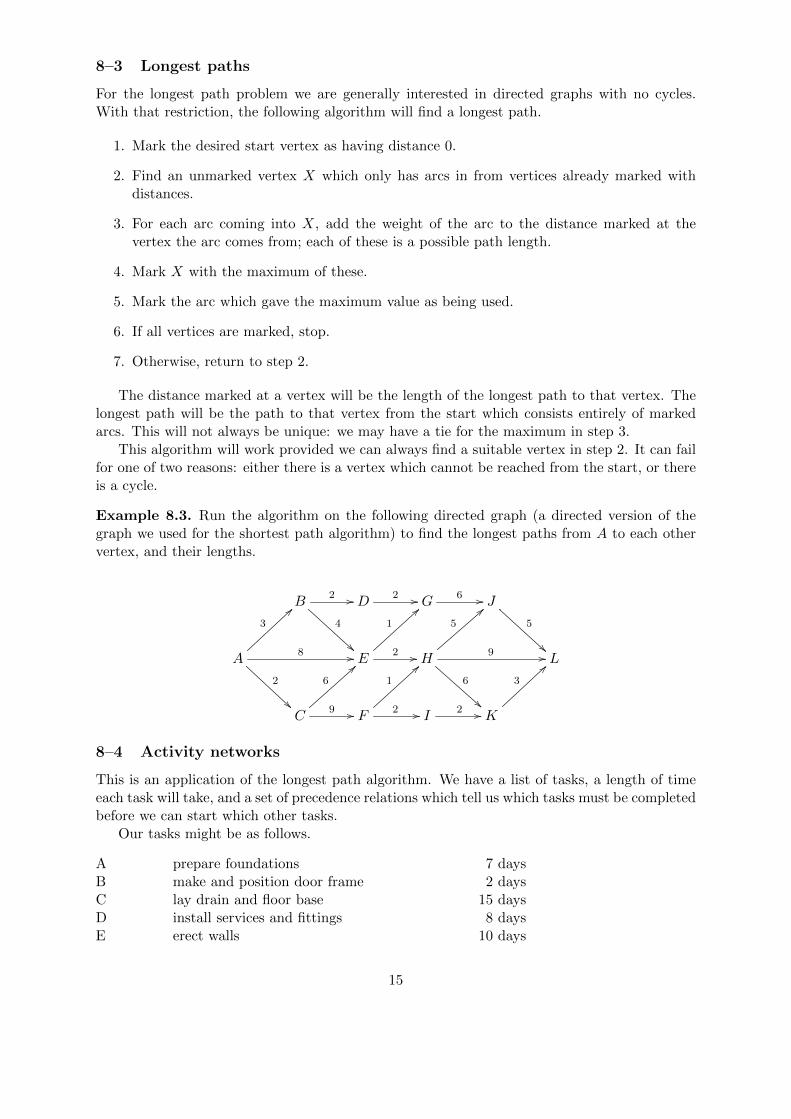
Example 8.3. Run the algorithm on the following directed graph (a directed version of thegraph we used for the shortest path algorithm) to find the longest paths from A to each othervertex, and their lengths.

B2 //

4

!!

D2 // G

6 // J

5

A

3

>>

8 //

2

E2 //

1

==

H

5

==

9 //

6

!!

L

C9 //

6

>>

F2 //

1

==

I2 // K

3

>>

8–4 Activity networks

This is an application of the longest path algorithm. We have a list of tasks, a length of timeeach task will take, and a set of precedence relations which tell us which tasks must be completedbefore we can start which other tasks.

Our tasks might be as follows.

A prepare foundations 7 daysB make and position door frame 2 daysC lay drain and floor base 15 daysD install services and fittings 8 daysE erect walls 10 days

15

F plaster ceiling 2 daysG erect roof 5 daysH install and paint doors and windows 8 daysI fit gutters and pipes 2 daysJ paint inside 3 days

The precedence relations are that D must come after E, E must come after A and B, F mustcome after D and G, G must come after E, H must come after G, I must come after C and F,and J must come after I.

What is the shortest time in which the structure can be built? We can solve such problemsusing Fulkerson’s algorithm.

1. Obtain a directed graph to represent the project. Put “start” in the first column. Findthe tasks which do not have any prerequisites and put them in the second column. Addarcs of weight 0 from “start” to each of them. In each subsequent column put all the taskswhich only have to follow tasks which already appear in earlier columns, and add an arcfor each precedence. Once all the tasks are included, put “end” in a final column and addan arc to “end” from every task which nothing has to follow. Each arc should be labelledwith the length of time taken by the task it is coming from. “Start” can be thought of asa task which takes no time but must occur before any other.

2. Use the longest path algorithm to find all the longest path distances from “start”. Theminimum time for completion is the length of the longest path to “end”, and the earliesttime at which each task may be begun is the length of the longest path to that task. Ifwe start the tasks at those times then we will always have completed all prerequisites bythe time we are due to start a given task.

3. If required, we may also work out the latest starting times (that is, the latest time a taskcan start if we are still to finish in the minimum time) by going backwards, column bycolumn. The latest time for “end” is the same as the earliest time. To get the latest timefor a task X, look at all the latest times of tasks which must follow X. Then subtract thetime taken for X from the smallest of these.

Example 8.4. Carry out all three parts of the algorithm for the tasks given above. The directedgraph we get will look like the following (labels omitted).

""

//

""start

;;

//

##

//

<<

//

<<

//::

// // end77

Remark. Some tasks give us no leeway: the earliest start time equals the latest start time. Werefer to the longest path from “start” to “end” as the critical path. All tasks on such a pathwill have equal start and end times, and so any delay on the critical path will delay the entireproject. The critical path might not be unique.

16

9 Planar graphs

An old puzzle concerns three houses which each need to be connected to three utilities. Is itpossible to connect each house to each utility without crossing the connections?

Definition 9.1. A planar graph is a graph which may be drawn in the plane without itsedges crossing. A plane graph is a specified drawing of a graph in the plane without edgescrossing.

In graph-theoretic terms, the puzzle is asking whether K3,3 is planar.

Theorem 9.2. The graphs K5 and K3,3 are not planar.

We will prove this in lectures

9–1 The planarity algorithm for Hamiltonian graphs

The proof we will give generalises to a way to check whether a Hamiltonian graph G is planar,provided we know or can easily find a Hamilton cycle.

1. Find a Hamilton cycle. Draw the vertices and edges of this cycle as a regular polygon,and draw the remaining edges as straight lines inside the polygon.

2. Draw the incompatibility graph, H. To do this, for each edge of G inside the cycle, giveH a vertex labelled by that edge; connect two vertices of H if the corresponding edges ofG cross in the drawing.

3. G is planar if and only if H is bipartite. If H is bipartite then we can draw G in theplane by putting the edges of G which correspond to red vertices of H inside the Hamiltoncycle, and those which correspond to blue vertices of H outside. Conversely, given a planedrawing of G we can colour vertices of H red if they correspond to edges inside the cycleand blue otherwise, and this will be a bipartition of H.

Example 9.3. Carry out the algorithm on the two graphs shown; step 1 has already beencarried out.

9–2 Kuratowski’s theorem

It is easy to see that any subgraph of a planar graph is also planar – start from a plane drawing ofthe original graph and rub out edges and vertices as appropriate. So any graph which containsa non-planar graph is not planar, and in particular any graph which contains K5 or K3,3 isnon-planar.

17

Kn is non-planar if n > 5 (but is planar if n < 5) and Kr,s isnon-planar if r, s > 3 (but is planar if r < 3). However, there are manynon-planar graphs which do not contain either K5 or K3,3 as asubgraph. The graph shown does not contain K5 (or K3,3), but itlooks like K5, and is non-planar for the same reason. This examplemotivates the following definition.

Definition 9.4. A subdivision of a graph G is any graph obtained by inserting new verticesof degree 2 along some of the edges; each edge can have any number of such vertices added.

In other words H is a subdivision of G if we can obtain H by replacing some of the edgesof G with paths. We interpret “some of the edges” above to include the case where none of theedges are modified, so that G is a subdivision of itself.

Suppose H is a subdivision of G. If G is planar then we may take a plane drawing of G andadd new vertices along the edges to get a plane drawing of H. Conversely, if H is planar wemay get a plane drawing of G by replacing the path of each subdivided edge by a single curve.

Since K5 and K3,3 are not planar, neither is any subdivision of either of them, and so neitheris any graph which contains a subdivision of K5 or K3,3. Remarkably, that is enough to give acomplete classification of planar graphs.

Theorem 9.5 (Kuratowski). A graph is planar if and only if it contains no subdivision of K5

or K3,3 as a subgraph.

We say two graphs G, H are homeomorphic if both are isomorphic to subdivisions ofthe same graph F . If H is a subdivision of G then G and H are homeomorphic (by takingF = G), but in general two graphs can be homeomorphic without either being isomorphic toa subdivision of the other. Kuratowski’s theorem may be equivalently stated as “A graph isplanar if and only if it contains no subgraph homeomorphic to K5 or K3,3.” We shall not proveKuratowski’s theorem here as the proof that any graph without such a subgraph is planar isvery complex.

Example 9.6. We previously used the planarity algorithmto show that the graph to the right is not planar.Consequently, by Kuratowski’s theorem, it must contain asubdivision of K5 or K3,3. Find such a subdivision.

9–3 Euler’s formula

Any plane graph G divides the plane into regions, called the faces of G. The region outside Gis counted as one of the faces. The degree of a face is the number of sides of edges boundingit (so that if an edge has the same face on both sides, it is counted twice in the degree). Likevertex degree, this satisfies a handshaking lemma.

Lemma 9.7. The sum of the face degrees of a plane graph is twice the number of edges.

18

Euler’s formula gives a relation between the number of edges, the number of faces and thenumber of vertices.

Theorem 9.8 (Euler). If a plane connected graph has v vertices, e edges and f faces thenv + f − e = 2.

We will prove this in lectures

For a fixed planar connected graph G, with v vertices and e edges, it follows that every planedrawing of G has e − v + 2 faces, so the number of faces of G does not depend on how it isdrawn in the plane.

Since the graph of any polyhedron is planar, the same formula applies to a polyhedron withv vertices, e edges and f faces. (Imagine a hollow rubber polyhedron. Puncture any face,stretch the hole and flatten the polyhedron onto the plane. The punctured face becomes theexternal face of a plane drawing of the graph.)

We can use Euler’s formula to bound the number of edges a planar graph can have.

Corollary 9.9. If G is a simple connected planar graph with v > 3 vertices and e edges thene 6 3v − 6. If additionally G has no cycle of length 3 then e 6 2v − 4.

We will prove this in lectures

Both bounds are best possible.

Example 9.10. Use these bounds to give another proof of the fact that K5 and K3,3 are notplanar.

9–4 Fullerenes

A fullerene is a polyhedral molecule consisting entirely ofcarbon atoms. The first such molecule to be synthesised,buckminsterfullerene, has 60 carbon atoms arranged in theform of a truncated icosahedron (the polyhedron used as abasis for the standard football design).

In any fullerene each atom is bonded to three others, and every face is either a hexagon or apentagon. We can think of this as a 3-regular plane graph with p faces of degree 5 and h facesof degree 6 (and no others).

Example 9.11. Prove that every fullerene has exactly 12 pentagonal faces.

A 20-carbon fullerene with 12 pentagonal faces and no hexagonal faces does exist, as do manyother fullerenes smaller than buckminsterfullerene, but they do not occur naturally whereas itdoes (and so do four others which are slightly larger). One reason for this is that configurationswhere two pentagonal faces share an edge are much less stable. What is the smallest fullerenein which no two pentagons share an edge? In fact no two pentagons can share a vertex, sincethe three faces meeting at each vertex all share edges, so the 12 pentagons must between themspan 60 different vertices. Buckminsterfullerene has 60 carbons and no two pentagons share anedge, so it is the smallest such fullerene.

19

9–5 Graphs on surfaces

What happens if instead of trying to draw graphs in the plane without edges crossing we try todraw them on some other surface? The graphs which can be drawn on a sphere without edgescrossing are just the planar graphs. Other surfaces, such as the torus, Mobius strip or Kleinbottle, might be more interesting.

We can represent the torus as a square with opposite sides identified – so that moving offthe left-hand side of the square brings us back onto the right-hand side, and likewise with thetop and bottom. We may represent the Mobius strip as a square with top and bottom identifiedwith a twist.

The diagram below shows how K5 may be drawn on the torus and Mobius strip withoutedges crossing. Edges which cross the sides of the squares have been marked to show how theyjoin up.

Example 9.12. Draw K3,3 on the torus and Mobius strip without edges crossing. For each ofthe four drawings, count the number of faces. Is Euler’s formula satisfied?

Definition 9.13. The orientable surface of genus g is the torus-like surface with g holes.

The orientable surface of genus 0 is a sphere, that of genus 1 is a normal torus, and so on.

Definition 9.14. The genus of a graph G is the smallest value of g such that G can be drawnon the orientable surface of genus g without edges crossing. We write g(G) for the genus of G.

Since any graph which can be drawn on the surface of genus g can also be drawn on thesurface of genus g + 1, we may equivalently say that G has genus g if it may be drawn on theorientable surface of genus g without edges crossing, but not on the orientable surface of genusg− 1. Euler’s formula works for the plane or sphere, i.e. for genus 0, but may be generalised tohigher genus. We won’t prove this generalisation.

Theorem 9.15. If G is a connected graph of genus g with v vertices and e edges, and is drawnon the orientable surface of genus g without crossings in such a way as to have f faces, thenv + f − e = 2− 2g.

The assumption that G has genus g is necessary; if we remove that condition then we insteadget v + f − e > 2− 2g.

Example 9.16. Let G be a simple connected graph of genus g with e edges and v > 3 vertices.Show that g > 1− v/2 + e/6. Use this inequality to show that g(Kn) > (n− 3)(n− 4)/12 (forn > 3).

20

In fact g(Kn) = d 112(n − 3)(n − 4)e for every n > 3 (where the notation dxe, pronounced

“ceiling of x”, means the smallest integer y with y > x). So g(K3) = g(K4) = 0, g(K5) =g(K6) = g(K7) = 1, g(K8) = 2.

One other surface we might consider is the Klein bottle, which islike a torus with a twist; we can represent it as shown.

Example 9.17. Draw K6 on the Klein bottle.

10 Vertex colouring

Let G be any graph. A vertex colouring of G is an assignment of a colour to each vertex suchthat every edge goes between two different colours. We often just call this a colouring of G.

We will generally focus on simple graphs when we talk about vertex colouring. If G has aloop then it has no colourings at all, and it makes no difference for colouring purposes whetherwe have one or two (or more) edges between x and y.

We say that G is k-colourable if it has a colouring which uses at most k colours. Note thata graph is bipartite if and only if it is 2-colourable; the definitions are the same.

Theorem 10.1. A graph is bipartite if and only if it has no cycle of odd length.

We will prove this in lectures; we need the following lemma

Lemma 10.2. Any closed walk with an odd number of edges contains an odd cycle.

Proof. Let H be the graph on the same vertex set with an edge between x and y for every timex and y appear consecutively in the walk (so if we use the same edge xy of G twice, there aretwo edges between x and y in H). All vertices have even degree in H, so by Lemma 4.2 theedges of H may be partitioned into disjoint cycles. If all these cycles are even then H wouldhave an even number of edges, which it doesn’t, so at least one must be odd.

Definition 10.3. The chromatic number of G, written χ(G), is the smallest k such that Gis k-colourable.

If χ(G) = k we sometimes say “G is k-chromatic”.

10–1 Bounds on the chromatic number

Let G be a simple graph. Choose an ordering of the vertices of G. We will colour the verticesone at a time in order with colours from the set 1, 2, 3, . . .. When colouring each vertex, wechoose the smallest colour which has not already been assigned to one of its neighbours. Thisis the greedy algorithm for colouring. It will always produce a colouring, but the number ofcolours used will depend on what order we colour the vertices in. There is always some orderfor which the greedy algorithm uses only χ(G) colours. On the other hand, the worst-caseperformance of the greedy algorithm can be very bad: for each n there is a bipartite graph on2n vertices and an ordering for which greedy uses n+ 1 colours.

21

Theorem 10.4. If G is a simple graph of maximum degree ∆ then χ(G) is at most ∆ + 1. Ifχ(G) = ∆ + 1 then G must have at least ∆ + 1 vertices of degree ∆.

We will prove this in lectures

The following theorem of Brooks, which we will not prove, is a stronger version of this.

Theorem 10.5 (Brooks). If G is a simple connected graph with maximum degree ∆ then eitherG = K∆+1, G is an odd cycle, or χ(G) 6 ∆.

10–2 Colouring on surfaces

A natural question is to ask whether we can bound the chromatic number of planar graphs. Itwas conjectured as early as 1852 that only four colours are needed to colour any simple planegraph, and several fallacious proofs were produced during the 19th century. In 1890, Heawoodshowed that an earlier “proof” by Kempe was incorrect, but adapted the method to prove thatfive colours are always sufficient. The conjecture itself was not proved until 1976, by Appel andHaken – the famous “four-colour theorem”. Their proof relied on complicated arguments toreduce the conjecture to almost 2000 different cases, which were then checked by computer.

It is quite easy to show that six colours are sufficient, using a simple consequence of Corollary9.9.

Lemma 10.6. Any simple planar graph has a vertex of degree at most 5.

Corollary 10.7. If G is a simple plane graph then χ(G) 6 6.

We will prove these in lectures

This method forms the basis of the next two results (both due to Heawood).

Theorem 10.8. If G is a simple plane graph then χ(G) 6 5.

Proof. Again, we use induction on the number of vertices; the result is true for graphs with 5 orfewer vertices. Suppose G has n vertices and assume the result is true for all graphs with fewervertices. By Euler’s formula, G has some vertex v with d(v) 6 5. If we remove v the remainingvertices may be coloured with 5 colours; take any such colouring. If this colouring does not useall 5 colours on the neighbours of v then there is a colour available for v and we are done. If notthen v has 5 neighbours all of different colours. Label these a1, . . . a5 going clockwise around vin our plane drawing, and assume ai has colour i for each i.

To complete the proof, we need to show that we can modify the colouring so that there willbe a colour available to use at v. We will do this part in lectures.

For planar graphs the lower bound (that 4 colours may be required) is trivial, but the upperbound (the four-colour theorem) is very hard. For other orientable surfaces, however, the upperbound is relatively easy whereas showing that this many colours may be required is hard. Wewill just prove the upper bound. Here bxc, “floor of x”, is the largest integer less than or equalto x.

Theorem 10.9 (Heawood’s bound). If G is a simple graph drawn on the surface of genus g,where g > 0, then χ(G) 6

⌊12

(7 +√

1 + 48g)⌋

.

22

Proof (non-examinable). Write h(g) =⌊

12

(7 +√

1 + 48g)⌋

. Again we prove the result by in-duction. As before, it is sufficient to show that any simple graph on this surface has a vertex ofdegree at most h(g)− 1. Suppose not; take a counterexample G. From Euler’s formula for thesurface, we can deduce e 6 3v + 6g − 6 (the equivalent of Corollary 9.5 for this surface). Sinceevery vertex has degree at least h(g), by handshaking 2e > h(g)v, so

v(h(g)− 6) 6 12g − 12 .

Since g > 1, h(g) − 6 > 0. Also, since G is simple and any vertex has degree at least h(g), wemust have v > h(g) + 1. So

(h(g) + 1)(h(g)− 6) 6 12g − 12 .

Now h(g) > 12

(7 +√

1 + 48g)− 1, and consequently(√

1 + 48g + 7)(√

1 + 48g − 7)< 48g − 48 ,

but in fact the two sides are equal.

Heawood conjectured that this bound was best possible for every g, i.e. that for every g > 1there exists a graph of genus g which requires h(g) colours. This is now known – it is the Ringel–Youngs Theorem – and the last remaining cases were proved in 1968. Heawood also proved asimilar bound for graphs which may be drawn on non-orientable surfaces, and conjectured thatit was best possible in every case. This conjecture is false for the Klein bottle (in 1930 Franklinshowed that any graph drawn on the Klein bottle can be coloured with 6 colours, whereasHeawood’s bound was 7), but has since been proved for every other non-orientable surface. Theanalogue of Euler’s formula on the Klein bottle is that v+ f − e > 0 (with equality if the graphcannot be drawn on a simpler surface).

Theorem 10.10 (Franklin). If the simple graph G can be drawn on the Klein bottle thenχ(G) ≤ 6.

Proof (non-examinable). We will show in lectures that if any 7-chromatic simple graph may bedrawn on the Klein bottle then K7 may be drawn on the Klein bottle in such a way that everyface is a triangle.

To complete the proof we must show that if K7 can be drawn on a surface in such a waythat every face has degree 3 and is simply connected then this surface must be the torus. Picka vertex, 1, and label its neighbours 2, . . . 7 clockwise.

23

What face meets face 123 at the edge 23? It cannot be 237, since we already have an edge27; it cannot be 234 either so it is 235 or 236. Without loss of generality (the other choice isequivalent to reflecting the diagram and relabelling) it is 235. Now everything else is determined,and our triangulation looks locally like the second diagram; identifying equal points makes atorus, as shown.

11 The chromatic polynomial

Previously we have considered the question of whether a given graph can be coloured with kcolours. Now we will think about how many ways there are to colour a given graph with kcolours. Let G be a simple graph, and write PG(k) for the number of ways of vertex-colouringG with k colours.

For the empty graph, PEn(k) = kn, since there are k choices at each vertex. For the completegraph, PKn(k) = k(k − 1)(k − 2) · · · (k − n + 1), because the first vertex can be coloured withany colour, the second with any other colour, the third with any colour not yet used, and so on.

Lemma 11.1. If T is a tree on n vertices then PT (k) = k(k − 1)n−1.

We will prove this in lectures

11–1 Techniques for calculating PG(k)

1. Disconnected graphs. If G = A tB then PG(k) = PA(k)PB(k), since we may colour eachpart separately.

2. Gluing together at a vertex. Suppose G is made up of two parts, G1 and G2, which sharea single vertex v. This time we can’t just colour G1 and G2 separately because we needto make sure both colourings give v the same colour. There are PG1(k) k-colourings ofG1; for each one there are 1

kPG2(k) colourings of G2 which give v the same colour, soPG(k) = 1

kPG1(k)PG2(k).

A special case of this rule is where G has a vertex of degree 1, and removing this vertexleaves the graph G1. In this case after colouring G1 we have k − 1 choices for the othervertex, so PG(k) = (k − 1)PG1(k).

3. Gluing together along an edge. Suppose G is made up of two parts, G1 and G2, withexactly two vertices in common, u and v, and G1, G2 and G all include the edge uv.Now our colourings must agree on u and v. Since u and v are adjacent, they must havedifferent colours in any colouring of G1 or G2, and any pair of different colours is equallylikely. Consequently PG(k) = 1

k(k−1)PG1(k)PG2(k).

Be careful to make sure that uv is an edge of the graph and that you include this edge inboth G1 and G2. A special case is where G has a vertex v of degree 2 and its neigbours havean edge between them. Then removing v leaves a graph G1 and PG(k) = (k − 2)PG1(k).

4. Suppose G has subgraphs G1 and G2 which between them include every edge and vertexof G, and G1∩G2

∼= Kr. Then PG(k) = PG1(k)PG2(k)/PKr(k). This is a generalisation ofthe previous rules, but is less often useful for higher r. The intersection being a completegraph is necessary for any rule of this type to work.

24

11–2 The contraction–deletion relation

What is PC4(k)? None of the above rules help, so we will need a new idea. To that end we willdefine several modifications to graphs.

Let G be a simple graph, and x, y be vertices. If x and y are not adjacent then G + xy isthe simple graph obtained by adding the edge xy; similarly, if x and y are adjacent then G−xyis the simple graph obtained by deleting the edge xy. If x and y are not adjacent then we mayidentify x and y to form the simple graph Gx=y. This only has a single vertex correspondingto x and y; this is adjacent to z if and only if z was adjacent to x or y in G (but we neverhave multiple edges, even if z was adjacent to both). Finally, if e is any edge of G then we maycontract e to form the simple graph G/e. To contract e, first delete e and then identify its twovertices.

Theorem 11.2. If G is a simple graph and x, y non-adjacent vertices then PG(k) = PG+xy(k)+PGx=y(k).

Corollary 11.3. If G is a simple graph and e is any edge of G then PG(k) = PG−e(k)−PG/e(k).

We will prove Theorem 11.2 in lectures

Corollary 11.3 follows immediately by applying Theorem 11.2 to G− e.This gives two recursive algorithms for finding the chromatic polynomial of any simple graph

G. Using Theorem 11.2, we can choose two non-adjacent vertices x and y, and form the graphsG1 = G + xy and G2 = Gx=y, so that PG = PG1 + PG2 . If G1 is now complete we know PG1 ;if not we choose two non-adjacent vertices in G1 and form two more graphs G3, G4 from itin the same way. Likewise if G2 is not complete we form graphs G5 and G6 from it, and nowPG = PG3 +PG4 +PG5 +PG6 . We continue this process until all remaining graphs are complete.

In fact, when performing this algorithm by hand we do not need to carry on until everythingis complete – if a graph with an easy to calculate chromatic polynomial comes up we just leaveit.

The other recursive algorithm is to use Corollary 11.3. Choose an edge e0 of G and writeG1 = G−e0, G2 = G/e0 so that PG = PG1−PG2 If G1 is not empty then we can choose anotheredge e1 in G1 and set G3 = G1 − e1, G4 = G1/e1, and similarly for G2. Then we have

PG = (PG3 − PG4)− (PG5 − PG6)

= PG3 − PG4 − PG5 + PG6 ;

we have to be careful to keep track of signs with this method. Continue until we have reducedto graphs whose chromatic polynomials we know – if implementing this on computer it may beeasier to continue until all remaining graphs are empty.

Example 11.4. Use each method in turn to find PC4(k), and checkthat the answers agree.

Example 11.5. Calculate the chromatic polynomials of the wheelW5 and the graph G shown.

11–3 Properties of the chromatic polynomial

We are now able to use Corollary 11.3 to prove that PG(k) has the following properties.

25

1. PG(k) is a polynomial in k.

2. Its degree is the number of vertices of G, n.

3. The coefficients are integers.

4. The coefficient of kn is 1.

5. The coefficient of kn−1 is −e(G).

6. The coefficients alternate in sign.

We only need a single method to prove all these facts. We will just prove properties 1 to5 in lectures, as including property 6 would make the proof unnecessarily fiddly (though notreally any harder).

Theorem 11.6. Let G be a simple graph with n vertices and m edges. Then PG(k) is apolynomial with integer coefficients of the form kn −mkn−1 + · · · .

We will prove this in lectures

12 Edge colouring

Let G be a graph with no loops (but multiple edges are permitted). An edge colouring of Gis as assignment of a colour to each edge such that any two edges which have a common vertexare assigned different colours. We say G is k-edge-colourable if there is an edge colouring of Gusing at most k colours and define the chromatic index of G, which we write χ′(G), to be thesmallest k for which G is k-edge-colourable.

Clearly if G has maximum degree ∆ then χ′(G) > ∆, since the ∆ edges meeting at a vertexof maximum degree all require different colours. A greedy-algorithm based argument wouldquickly give χ′(G) 6 2∆, since each edge shares a vertex with at most 2∆− 1 others, but if Gis simple then much more is true.

Theorem 12.1 (Vizing). If G is a simple graph with maximum degree ∆ then χ′(G) 6 ∆ + 1.

We will not prove Vizing’s Theorem. The requirement that G is simple is necessary: forgraphs with multiple edges, χ′(G) can be as large as 3∆/2. If G is simple then χ′(G) is either∆ or ∆ + 1, but it is in general difficult to determine which. We will determine which it is in afew special cases, however.

Lemma 12.2. Let G be a ∆-regular simple graph with n vertices. If n is odd then χ′(G) > ∆.

We will prove this in lectures

A natural application of edge colouring is tournament scheduling. Imagine a league of nplayers in which every player plays against every other once. How many rounds are needed toschedule all the games? The answer is χ′(Kn) – the edges represent matches and the colour ofan edge is the round in which that match occurs.

Theorem 12.3. If n is odd then χ′(Kn) = n; if n is even then χ′(Kn) = n− 1.

26

Proof. By Lemma 12.2, χ′(Kn) > n if n is odd, and by Vizing’s Theorem χ′(Kn) 6 n, socertainly χ′(Kn) = n if n is odd. So we just need to construct an edge colouring of Kn withn− 1 colours when n is even to complete the proof. In fact we will give a construction with ncolours for n odd as well. We will complete this in lectures.

We can also determine the chromatic index for any bipartite graph. The proof is non-examinable, but included for interest.

Theorem 12.4. If G is bipartite with maximum degree ∆ then χ′(G) = ∆.

Proof (non-examinable). This proof uses a modification of Kempe chains. We prove it by in-duction on the number of edges; it is certainly true for a graph with 1 edge. Suppose it istrue for any bipartite graph with fewer edges than G, and remove an edge xy from G to get abipartite graph G′ with fewer edges and maximum degree at most ∆. Choose an edge colouringof G′ with ∆ colours and try to extend it to an edge colouring of G. Now x had degree at most∆ in G so has degree at most ∆− 1 in G′, so there is some colour which has not yet been usedat x, 1, say. Likewise there is some colour which hasn’t been used at y. If this is also 1 we aredone, so suppose it is 2. We want to colour the edge xy with colour 1, so we try to swap somecolours in such a way that 1 becomes available at y, while still being available at x.

Construct a path from y whose edges are alternately coloured 1 and 2 which is as long aspossible. This path is unique: if we have reached z and are looking for an edge of colour 1 thenthere is at most one since we have a valid edge colouring. If it does not reach x then we canjust swap all the colours along the path to get a new colouring in which 1 is available at x andy, which we can extend to a colouring of G. But the path cannot reach x after an odd numberof edges, since then the edge reaching x would be colour 1, which we assumed was available atx. It cannot reach x after an even number of vertices either, since then these edges togetherwith xy would be an odd cycle in G, and G is bipartite. So the path does not reach x and wecan swap the colours on it as required.

13 Face colouring

We stated the four-colour theorem as a result on vertex colouring, but it was originally con-jectured as a result on face-colouring. A face-colouring of a bridgeless plane graph is anassignment of colours to faces such that two faces which meet along an edge have differentcolours. We require graphs to be bridgeless so that no face meets itself along an edge.

Theorem 13.1. A bridgeless plane graph G is face-colourable with two colours if and only ifevery vertex has even degree.

We will prove this in lectures

Given a connected plane graph G we may define its dual G∗ as follows. Pick a point insideeach face of G; these will be the vertices of G∗. For each edge e of G we draw a correspondingedge of G∗ between the vertices corresponding to faces on either side of e, which crosses e. Notethat G∗ is defined only for a particular plane drawing of G, and we define not just the graph G∗

but also a plane drawing of it. The drawing we use for G does matter: it is easy to constructplane graphs G and H such that G ∼= H but G∗ H∗.

Provided G is connected G∗ satisfies the following conditions.

a G∗ is connected.

27

b (G∗)∗ = G.

c G∗ has no loops ⇐⇒ G has no bridges.

d If G has v vertices, e edges and f faces then G∗ has f vertices, e edges and v faces.

Consequently we may state the four-colour theorem in either of the following equivalent forms.

1. Every loopless planar graph is 4-colourable.

2. Every bridgeless plane graph is 4-face-colourable.

In fact, given any bridgeless planar graphG we may construct a 3-regular bridgeless planar graphwhich is at least as hard to face-colour. G has no vertices of degree 1, because it is bridgeless,and any vertex of degree 2 may be replaced by a single edge connecting its neighbours, withoutaffecting which faces meet. Any vertex of degree at least 4 may be truncated as shown; anyk-face-colouring of the truncated graph contains a k-face-colouring of the original graph.

Consequently the four-colour theorem is equivalent to

3. Every 3-regular bridgeless plane graph is 4-face-colourable.

Our final result links the 4-colour theorem to edge colouring.

Theorem 13.2 (Tait). The following are equivalent:

3. Every 3-regular bridgeless plane graph is 4-face-colourable.

4. Every 3-regular bridgeless plane graph is 3-edge-colourable.

The proof of this result is non-examinable; we will only prove in lectures that (3)⇒ (4).The four-colour theorem means that any bridgeless planar cubic graph must be 3-edge-

colourable. The planarity condition is necessary; perhaps the best-known counterexample ingraph theory is the Petersen graph, which is bridgeless and 3-regular but not 3-edge-colourable(in addition to many other remarkable properties).

28