Graph Theory

Frank de Zeeuw

August 17, 2016

1 Introduction 31.1 Definitions . . . . . . . . . . . . . . . . . . . . . . . . . . . . . . . . . . . . 31.2 Basic facts . . . . . . . . . . . . . . . . . . . . . . . . . . . . . . . . . . . . 5

2 Trees 72.1 Basic facts . . . . . . . . . . . . . . . . . . . . . . . . . . . . . . . . . . . . 72.2 Spanning trees and basic algorithms . . . . . . . . . . . . . . . . . . . . . . 82.3 Distances and breadth-first search . . . . . . . . . . . . . . . . . . . . . . . 92.4 Minimum-weight spanning trees . . . . . . . . . . . . . . . . . . . . . . . . 10

3 Matchings 123.1 Matchings and augmenting paths . . . . . . . . . . . . . . . . . . . . . . . 123.2 Hall’s Theorem . . . . . . . . . . . . . . . . . . . . . . . . . . . . . . . . . 133.3 Konig’s Theorem . . . . . . . . . . . . . . . . . . . . . . . . . . . . . . . . 14

4 Covers and independent sets 164.1 Summary of matchings in arbitrary graphs . . . . . . . . . . . . . . . . . . 164.2 Matchings, covers, and independent sets . . . . . . . . . . . . . . . . . . . 164.3 Independent sets . . . . . . . . . . . . . . . . . . . . . . . . . . . . . . . . 184.4 Dominating sets . . . . . . . . . . . . . . . . . . . . . . . . . . . . . . . . . 19

5 Coloring 215.1 Vertex coloring . . . . . . . . . . . . . . . . . . . . . . . . . . . . . . . . . 215.2 Edge coloring . . . . . . . . . . . . . . . . . . . . . . . . . . . . . . . . . . 225.3 Line graphs . . . . . . . . . . . . . . . . . . . . . . . . . . . . . . . . . . . 24

6 Hamilton cycles 266.1 Girth and circumference . . . . . . . . . . . . . . . . . . . . . . . . . . . . 266.2 Hamilton cycles . . . . . . . . . . . . . . . . . . . . . . . . . . . . . . . . . 276.3 Sufficient conditions . . . . . . . . . . . . . . . . . . . . . . . . . . . . . . . 28

7 2-connected graphs 307.1 2-connectedness . . . . . . . . . . . . . . . . . . . . . . . . . . . . . . . . . 307.2 Whitney’s Theorem . . . . . . . . . . . . . . . . . . . . . . . . . . . . . . . 317.3 3-connectedness and Brooks’s Theorem . . . . . . . . . . . . . . . . . . . . 32

These are lecture notes from the class Graph Theory that I taught at EPFL in Spring 2016.

1

8 k-connected graphs 348.1 Menger’s Theorem . . . . . . . . . . . . . . . . . . . . . . . . . . . . . . . 348.2 k-connected graphs . . . . . . . . . . . . . . . . . . . . . . . . . . . . . . . 35

9 Planar graphs 389.1 Drawings of graphs . . . . . . . . . . . . . . . . . . . . . . . . . . . . . . . 389.2 Non-planar graph . . . . . . . . . . . . . . . . . . . . . . . . . . . . . . . . 389.3 Euler’s formula . . . . . . . . . . . . . . . . . . . . . . . . . . . . . . . . . 399.4 Coloring planar graphs . . . . . . . . . . . . . . . . . . . . . . . . . . . . . 41

10 Extremal graph theory I 4210.1 Extremal graph theory . . . . . . . . . . . . . . . . . . . . . . . . . . . . . 4210.2 Triangles . . . . . . . . . . . . . . . . . . . . . . . . . . . . . . . . . . . . . 4310.3 Squares . . . . . . . . . . . . . . . . . . . . . . . . . . . . . . . . . . . . . 4410.4 Trees . . . . . . . . . . . . . . . . . . . . . . . . . . . . . . . . . . . . . . . 46

11 Extremal graph theory II 4811.1 Complete graphs . . . . . . . . . . . . . . . . . . . . . . . . . . . . . . . . 4811.2 Complete bipartite graphs . . . . . . . . . . . . . . . . . . . . . . . . . . . 51

12 Ramsey theory 5412.1 Ramsey numbers . . . . . . . . . . . . . . . . . . . . . . . . . . . . . . . . 5412.2 Bounds for R(Kt, Kt) . . . . . . . . . . . . . . . . . . . . . . . . . . . . . . 5512.3 A general Ramsey theorem . . . . . . . . . . . . . . . . . . . . . . . . . . . 57

2

Chapter 1

Introduction

1.1 Definitions

Definition. A graph G = (V,E) consists of a finite set V and a set E of two-elementsubsets of V . The elements of V are called vertices and the elements of E are callededges.

For instance, very formally we can introduce a graph like this:

V = {1, 2, 3, 4}, E = {{1, 2}, {3, 4}, {2, 3}, {2, 4}}.

In practice we more often think of a drawing like this:

1 2

34

Technically, this is what is called a labelled graph, but we often omit the labels. When wesay something about an unlabelled graph like , we mean that the statement holds forany labelling of the vertices.

Here are two examples of related objects that in this course we do not consider graphs:

The first is a multigraph, which can have multiple edges and loops; the correspondingdefinition would allow the edge set and the edges to be multisets. The second is a directedgraph, in which every edge has a direction; in the corresponding definition the edgeswould be ordered pairs instead of two-element subsets. In this course we mostly avoidthese variants for simplicity, although they are certainly very useful objects. Most factsabout graphs in our sense have analogues for multigraphs or directed graphs, althoughthose are often a bit less nice. Another type of graph that we are avoiding is infinitegraphs ; many facts about finite graphs do not extend to infinite graphs.

Some notation: Given a graph G, we write V (G) for the vertex set, and E(G) for theedge set. For an edge {x, y} ∈ E(G), we usually write xy, and we consider yx to be thesame edge. If xy ∈ E(G), then we say that x, y ∈ V (G) are adjacent or connected or thatthey are neighbors. If x ∈ e, then we say that x ∈ V (G) and e ∈ E(G) are incident.

3

Definition (Subgraphs). Two graphs G,G′ are isomorphic if there is a bijection ϕ :V (G) → V (G′) such that xy ∈ E(G) if and only if ϕ(x)ϕ(y) ∈ E(G′). A graph H is asubgraph of a graph G, denoted H ⊂ G, if there is a graph H ′ isomorphic to H such thatV (H ′) ⊂ V (G) and E(H ′) ⊂ E(H).

With this definition we can for instance say that is a subgraph of . As mentionedabove, when we talk about graphs we often omit the labels of the vertices. A more formalway of doing this is to define an unlabelled graph to be an isomorphism class of labelledgraphs. We will be somewhat informal about this distinction, since it rarely leads toconfusion.

Definition (Degree). Fix a graph G = (V,E). For v ∈ V , we write

N(v) = {w ∈ V : vw ∈ E}

for the set of neighbors of v (which does not include v). Then d(v) = |N(v)| is the degreeof v. We write δ(G) for the minimum degree of a vertex in G, and ∆(G) for the maximumdegree.

Definition (Examples). The following are some of the most common types of graphs.

• Paths are the graphs Pn of the form . The graph Pn has n edges andn+ 1 vertices; we call n the length of the path.

• Cycles are the graphs Cn of the form . The graph Cn has n edges and nvertices; we call n the length of the cycle.

• Complete graphs are the graphs Kn on n vertices in which all vertices are adjacent.The graph Kn has

(n2

)edges. For instance, K4 is .

• Complete bipartite graphs are the graphs Ks,t with a partition V (Ks,t) = X ∪ Ywith |X| = s, |Y | = t, such that every vertex of X is adjacent to every vertex of Y ,and there are no edges inside X or Y . Then Kst has st edges. For example, K2,3 is

.

The following are the most common properties of graphs that we will consider.

Definition (Regular). A graph G is k-regular if d(v) = k for all v ∈ V (G).

Definition (Bipartite). A graph G is bipartite if there is a partition V (G) = X ∪ Ysuch that every edge of G has one vertex in X and one in Y ; we call such a partition abipartition.

Definition (Connected). A graph G is connected if for all x, y ∈ V (G) there is a pathin G from x to y (more formally, there is a path Pk which is a subgraph of G and whoseendpoints are x and y).A connected component of G is a maximal connected subgraph of G (i.e., a connected sub-graph that is not contained in any larger connected subgraph). The connected componentsof G form a partition of V (G).

4

1.2 Basic facts

In this section we prove some basic facts about graphs. It is a somewhat arbitrarycollection of statements, but we introduce them here to get used to the terminologyand to see some typical proof techniques.

Proposition 1.2.1. In any graph G we have∑

v∈V (G)

d(v) = 2|E(G)|.

Proof. We double count the number of pairs (v, e) ∈ V (G) × E(G) such that v ∈ e. Onthe one hand, a vertex v is involved in d(v) such pairs, so the total number of such pairs is∑

v∈V (G) d(v). On the other hand, every edge is involved in two such pairs, so the number

of pairs must equal 2|E(G)|.

This fact is sometimes called the “handshake lemma” because it says that at a partythe number of shaken hands is twice the number of handshakes. It has useful corollaries,such as the fact that the number of odd-degree vertices in a graph must be even.

The next lemma gives a condition under which a graph must contain a long path orcycle. Note that “contains a path” means that the graph has a subgraph that is isomorphicto some Pn, and similarly for cycles. The proof is an example of an extremal argument,where we take an object that is extremal with respect to some property, and show thatthis extremality implies some other property of the object.

Proposition 1.2.2. A graph G with minimum degree δ(G) ≥ 2 contains a path of lengthat least δ(G) and a cycle of length at least δ(G) + 1.

Proof. Let v1 · · · vk be a maximal path in G, i.e., a path that cannot be extended. Thenany neighbor of v1 must be on the path, since otherwise we could extend it. Since v1 hasat least δ(G) neighbors, the set {v2, . . . , vk} must contain at least δ(G) elements. Hencek ≥ δ(G) + 1, so the path has length at least δ(G).

To find a long cycle, we continue the proof above. The neighbor of v1 that is furthestalong the path must be vi with i ≥ δ(G) + 1. Then v1 · · · viv1 is a cycle of length at leastδ(G) + 1.

Note that in general these bounds cannot be improved, because Kδ+1 has minimumdegree δ, but its longest path has length δ and its longest cycle has length δ + 1. InProblem Set 1 we will see that we can find longer paths in graphs that are not complete.

The following lemma can be helpful when trying to prove certain statements for generalgraphs that are easier to prove for bipartite graphs. The lemma says that you don’t haveto remove more than half the edges of a graph to make it bipartite. The proof is anexample of an algorithmic proof, where we prove the existence of an object by giving analgorithm that constructs such an object.

Proposition 1.2.3. Any graph G contains a bipartite subgraph H with |E(H)| ≥ |E(G)|/2.

Proof. We prove the stronger claim that G has a bipartite subgraph H with V (H) = V (G)and dH(v) ≥ dG(v)/2 for all v ∈ V (G). Starting with an arbitrary partition V (G) = X∪Y(which need not be a bipartition for G), we apply the following procedure. We refer to Xand Y as “parts”. For any v ∈ V (G), we see if it has more edges to X or to Y ; if it hasmore edges that connect it to the part it is in than it has edges to the other part, then wemove it to the other part. We repeat this until there are no more vertices v that shouldbe moved.

5

There are at most |V (G)| consecutive steps in which no vertex is moved, since if noneof the vertices can be moved, then we are done. When we move a vertex from one partto the other, we increase the number of edges between X and Y (note that a vertex maymove back and forth between X and Y , but still the total number of edges between X andY increases in every step). It follows that this procedure terminates, since there are onlyfinitely many edges in the graph. When it has terminated, every vertex in X has at leasthalf its edges going to Y , and similarly every vertex in Y has at least half its edges goingto X. Thus the graph H with V (H) = V (G) and E(H) = {xy ∈ E(G) : x ∈ X, y ∈ Y }has the claimed property that dH(v) ≥ dG(v)/2 for all v ∈ V (G).

The last lemma gives a characterization of bipartite graphs. An “odd cycle” is just acycle whose length is odd. Again we give an algorithmic proof.

Proposition 1.2.4. A graph is bipartite if and only if it contains no odd cycle.

Proof. Suppose that G is bipartite with bipartition V (G) = X ∪ Y , and that v1 · · · vkv1

is a cycle in G, with v1 ∈ X. We must have vi ∈ X for all odd i and vi ∈ Y for all even i.Since vk is adjacent to v1, it must be in Y , so k must be even and the cycle is not odd.

Suppose we have a connected graph G which has no odd cycles. We can obtain abipartition using the following algorithm. Start with X, Y being empty sets. Pick anarbitrary vertex x0 and put it in X. Put all the neighbors of x0 in Y . For each y ∈ Y ,put into X all neighbors of y that have not yet been assigned. Then for each x ∈ X,put into Y all neighbors that have not yet been assigned. Keep repeating this until allvertices have been assigned. This algorithm is well-defined because no vertex is assignedmore than once (thanks to the stipulation that we only consider unassigned vertices). Itremains to be shown that the algorithm terminates (i.e., it does not go on endlessly), andthat the resulting partition is really a bipartition of V (G).

The algorithm terminates because G is connected (by assumption). Indeed, this meansthat every y ∈ Y has a path yv1 · · · vkx0 to x0, and in every step at least one more vertexfrom this past must get assigned.

Next we show that V (G) = X∪Y is a bipartition. Suppose that two vertices x1, x2 ∈ Xare adjacent. By construction, there is a path P from x1 to x0 that uses only edges betweenX and Y , and similarly there is such a path P ′ from x2 to x0; note that these paths mayintersect, so their union might not be a path. Let x3 be the first vertex where P intersectsP ′ (this could be x0). Then we get a path P ′′ from x1 to x3 to x2 that also has theproperty that all its edges are between X and Y . Since this path goes from X to X usingonly edges between X and Y , it must have an even number of edges. Thus, if we combineit with x1x2, we get an odd cycle, which is a contradiction. Similarly, if y1, y2 ∈ Y areadjacent, combining this edge with the path from y1 to y2 gives an odd cycle. This showsthat all edges of G are between X and Y , so G is bipartite.

We did the above under the assumption that G is connected. If it is not, we can applythe above to each connected component, and arbitrarily combine the bipartitions of thecomponents to get a bipartition of G.

6

Chapter 2

Trees

2.1 Basic facts

Definition. A tree is a connected graph without cycles. A forest is a graph without cycles.In a tree or a forest, a vertex of degree one is called a leaf.

Proposition 2.1.1. Every tree with at least two vertices has a leaf.

Proof. Take a longest path x0x1 · · ·xk in the tree (so k ≥ 1, since the tree has at leasttwo vertices). A neighbor of x0 cannot be outside the path, since then the path couldbe extended. But if x0 were adjacent to xi for some i > 1, then x0x1 · · ·xix0 would be acycle. So the only neighbor of x0 is x1, and x0 is a leaf. (Of course, the same works forxk, so there are at least two leaves.)

Proposition 2.1.2. Any tree T satisfies |E(T )| = |V (T )| − 1.

Proof. We use induction on the number of vertices. If |V (T )| = 1, then |E(T )| = 0.Otherwise, Proposition 2.1.1 gives a leaf x0 of T . Let T ′ be the graph obtained byremoving x0 and its only edge. Then T ′ is connected, since for any x, y ∈ V (T ′) thereis a path from x to y in T , and this path cannot pass through x0, so it is also a pathin T ′. Since T has no cycles, neither does T ′, so T ′ is a tree. By induction we have|E(T ′)| = |V (T ′)| − 1, so plugging in |E(T ′)| = |E(T )| − 1 and |V (T ′)| = |V (T )| − 1 givethe desired formula.

Corollary 2.1.3. Any forest F satisfies |E(F )| = |V (F )| − c(F ), where c(F ) is thenumber of connected components of F .

Proof. Each connected component T of F is a tree, so Proposition 2.1.2 gives |E(T )| =|V (T )| − 1. Summing up over the c(F ) components gives the desired formula.

Proposition 2.1.4. A graph G is a tree if and only if for all x, y ∈ V (G) there is aunique path between x and y.

Proof. First suppose we have a graph G in which any two vertices are connected by aunique path. ThenG is certainly connected. Moreover, ifG contained a cycle x0x1 · · ·xkx0,then x0xk and x0x1 · · ·xk would be two distinct paths between x0 and xk. Hence G is atree.

Suppose G is a tree and x, y ∈ V (G). Since G is connected, there is at least one pathfrom x to y. Suppose there are two paths P 6= P ′ from x to y. If these paths only intersect

7

at x and y, we can immediately combine them into a cycle, but in general the paths couldintersect in a complicated way, so we have to be careful. The paths P and P ′ could startout from x being the same; let u be the last vertex at which they are the same. Let v bethe first vertex after u on P that is again on P ′. Then there is a cycle that goes along Pfrom u to v, and then back along P ′ from v to u. This is a contradiction, so there is aunique path from x to y in G.

We introduce some notation for adding and removing edges in graphs. Given a graphG, we write G+xy for the graph with vertex set V (G)∪{x, y} and edge set E(G)∪{xy}(one or both of x, y could already be in G). We also write G − xy for the graph withvertex set V (G) and edge set E(G)\{xy}.

Proposition 2.1.5. Let T be a tree. If xy ∈ E(T ), then T − xy is not connected. Ifxy 6∈ E(T ) and x, y ∈ V (T ), then T + xy contains a unique cycle.

Proof. Let xy ∈ E(T ). Suppose that T − xy is connected. Then there is a path inT − xy from x to y. Combining this path with xy gives a cycle contained in T , which isa contradiction.

Let xy 6∈ E(T ) and x, y ∈ V (T ). By Proposition 2.1.4, there is a unique path in Tfrom x to y. Combining this path with xy gives a cycle in T + xy. If there were a secondcycle in T +xy, it would also have to contain xy. Then removing xy from this cycle wouldgive a second path from x to y in T , contradicting the uniqueness of the path.

2.2 Spanning trees and basic algorithms

Definition. A spanning tree of a graph G is a tree T with |V (T )| = |V (G)|.

Proposition 2.2.1. A graph G is connected if and only if it has a spanning tree.

Proof. If G contains a spanning tree T , then any two vertices in V (G) are connected bya path in T , which is also a path in G. Therefore G is connected.

IfG is connected, the following algorithm shows thatG has a spanning tree. Arbitrarilypick x ∈ V (G) and consider it as a tree T . Repeat the following for as long as possible.For every y ∈ V (G)\V (T ), check if y is adjacent to a vertex z in V (T ), and if so, replaceT by T + yz.

The algorithm continues until V (T ) = V (G), at which point T is a spanning tree.Indeed, it is a tree since every edge that we add has exactly one endpoint in the tree. It isspanning, because if there is still a vertex y ∈ V (G)\V (T ) when the algorithm terminates,then the connectedness of G implies that there is a path from y to x. Somewhere on thispath there must be a vertex v of T adjacent to a vertex w not in T , so the algorithm canstill add w, and cannot have terminated.

The proof of Proposition 2.2.1 gives a very simple algorithm for finding a spanningtree. It is of course not defined very formally; in particular, we did not specify how to picky. We could do that by putting an arbitrary order on V (G), and going over the verticesin that order.

Using this informal algorithm, we can give algorithms for the following basic tasks.

• Determine if G is connected: If the algorithm from the proof of Proposition 2.2.1finds a tree T with V (T ) = V (G), then G is connected; otherwise G is disconnected.

8

• Find the connected components of G: For a graph that is not connected, the algo-rithm will find a spanning tree of a connected component of G; repeat this to getall the components.

• Determine if G contains a cycle: Find the connected components. If some connectedcomponent H has |E(H)| 6= |V (H)|−1, then it contains a cycle, because it containsa spanning tree and at least one more edge. If |E(H)| = |V (H)| − 1 for everycomponent, then each component is equal to its own spanning tree, so the graphhas no cycle.

2.3 Distances and breadth-first search

We saw one way of obtaining a spanning tree of a graph, but this is certainly not the onlyway. We will now see a more specific algorithm that gives a spanning tree with specialproperties, called a breadth-first search tree or BFS tree. This algorithm lets us answervarious natural questions, like determining the distance between two vertices.

Definition. Let G be a graph. For two vertices x, y ∈ V (G), the distance d(x, y) =dG(x, y) is the length of a shortest path between x and y.The diameter of G is the length of the longest shortest path: diam(G) = maxx,y∈V (G) d(x, y).

Given a graph G and a subgraph H ⊂ G, we define

∂(H) = {xy ∈ E(G) : x ∈ V (H), y 6∈ V (H)}

for the set of edges going from vertices of H to vertices not in H. The algorithm in theproof of Proposition 2.2.1 worked by repeatedly adding an edge from ∂(T ) to the currenttree T . Another bit of terminology: To single out one vertex of a tree, we refer to it as aroot.

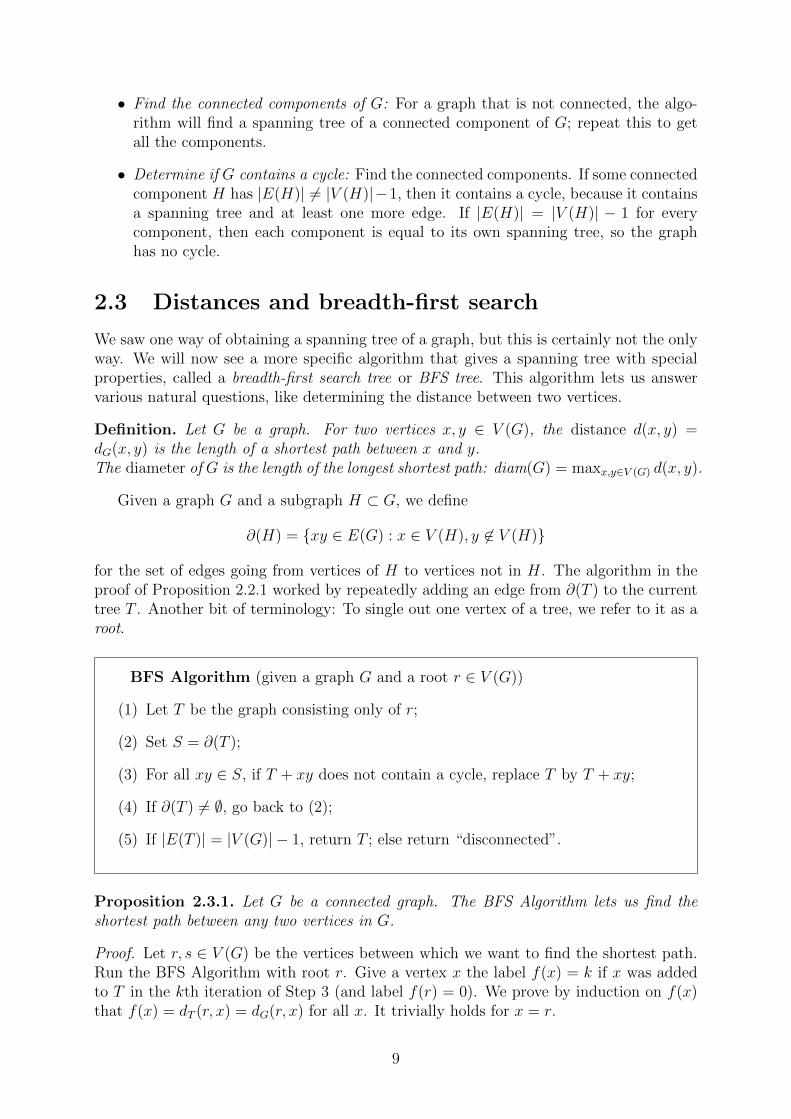
BFS Algorithm (given a graph G and a root r ∈ V (G))

(1) Let T be the graph consisting only of r;

(2) Set S = ∂(T );

(3) For all xy ∈ S, if T + xy does not contain a cycle, replace T by T + xy;

(4) If ∂(T ) 6= ∅, go back to (2);

(5) If |E(T )| = |V (G)| − 1, return T ; else return “disconnected”.

Proposition 2.3.1. Let G be a connected graph. The BFS Algorithm lets us find theshortest path between any two vertices in G.

Proof. Let r, s ∈ V (G) be the vertices between which we want to find the shortest path.Run the BFS Algorithm with root r. Give a vertex x the label f(x) = k if x was addedto T in the kth iteration of Step 3 (and label f(r) = 0). We prove by induction on f(x)that f(x) = dT (r, x) = dG(r, x) for all x. It trivially holds for x = r.

9

If f(x) = k, then by construction x is adjacent (in T and G) to a vertex y withf(y) = k − 1, and by induction we have dT (r, y) = dG(r, y) = k − 1. So there is a path(in T and G) of length k − 1 from r to y, which gives a path (in T and G) of length kfrom r to x. Moreover, there cannot be a shorter path in G from r to x, because thendG(r, x) < k, so by induction we would have f(x) = dG(r, x) < k, a contradiction.

Knowing that dT (r, x) = dG(r, x), we can find the shortest path from r to x in G byfinding the shortest path in T . To do that, we have to keep track of the “predecessor” ofeach x that we add in step (3); i.e., the vertex p with f(p) = f(x)− 1 that x is connectedto. Then, to find the shortest path from r to s, we start from s and repeatedly take thepredecessor, until we reach r.

Aside from letting us find shortest paths, the BFS algorithm lets us compute distances,and it also gives us algorithms for the following tasks on G.

• Compute diam(G): For each pair of vertices, we can find a shortest path and thusthe distance. Do this for all pairs and take the largest distance.

• Find a shortest cycle in G: For every edge xy, find a shortest path between x and yin G− xy (if it exists); combine this path with xy to get a cycle. Compare all thesecycles to find the shortest.

Some of these algorithms are very inefficient, but they are already much better thanbrute force approaches that go over all possible answers. There are all kinds of algorithmsthat do these tasks faster, but in this course, we don’t care too much about efficiency,and we focus on the graph-theoretical aspects (in particular, proving that the algorithmswork). For more sophisticated algorithms, we suggest taking a course in CombinatorialOptimization.

The problem of finding a shortest path is more interesting if we have a weight functionw : E(G)→ R+, and we want a path P for which the total weight

∑e∈P w(e) is minimal.

The BFS algorithm above does not do this, because it finds a path with the fewest edges,whereas a minimum-weight path may use many lightweight edges. Nevertheless, the bestknown algorithm for finding minimum-weight paths, known as Dijkstra’s algorithm, isbased on this BFS approach.

2.4 Minimum-weight spanning trees

Another natural algorithmic problem is the minimum-weight spanning tree problem. Fora graph G with a weight function w : E(G)→ R+, we want a spanning tree T whose totalweight w(T ) =

∑e∈E(T )w(e) is minimal (or determine that there is none, which means

G is disconnected). It is easy to imagine an application with locations that have to beconnected by a network of roads, which has to be done with the total road length as smallas possible.

The easiest thing to try is what is called a “greedy” approach: Repeatedly add thesmallest edge, while preserving connectedness and acyclicity (i.e., maintain a tree allalong).

Greedy Tree-Growing Algorithm

10

(1) Start with T being any vertex;

(2) Find e ∈ ∂(T ) with minimum w(e); if ∂(T ) = ∅, go to (4);

(3) Replace T by T + e; go to (2);

(4) If |E(T )| = |V (G)| − 1, return T , else return “disconnected”.

Theorem 2.4.1. The Tree-Growing Algorithm returns a minimum spanning tree, if itexists.

Proof. Suppose the algorithm returns T , and let e1, . . . , en−1 be the order in which theedges of T are selected. Let T ∗ be a minimum-weight spanning tree that shares as manyinitial vertices with T as possible; in other words, to each minimum-weight spanning treeT ∗ associate the smallest i such that ei 6∈ T ∗, and choose the T ∗ with the largest i. IfT = T ∗, then we are done, so assume T 6= T ∗.

Let e be the first edge not in T ∗ that was picked by the algorithm, and let T ′ bethe tree that the algorithm had before it picked e. Since e 6∈ T ∗, adding e to T ∗ createsa unique cycle by Proposition 2.1.5. There must be an edge f 6= e in that cycle forwhich f ∈ ∂(T ′), since the cycle leaves T ′ via e and must somehow re-enter T ′. Since thealgorithm chose e over f , we must have w(e) ≤ w(f).

Now T ∗∗ = T ∗ + e − f is a tree (because the unique cycle containing e is broken byremoving f) with w(T ∗∗) ≤ w(T ∗), so T ∗∗ is also a minimum-weight spanning tree. ButT ∗∗ shares more initial vertices with T than T ∗, contradicting the definition of T ∗. Itfollows that T = T ∗, and T is minimum.

There are different greedy approaches for finding a minimum spanning tree, where adifferent property is preserved in the process. In Problem Set 2, we will see two suchalgorithms, one that greedily grows a forest, and one that greedily removes edges whilekeeping the graph connected.

11

Chapter 3

Matchings

3.1 Matchings and augmenting paths

Definition. Let G be a graph. A set of edges M ⊂ E(G) is a matching if no two edgesin M share a vertex. A matching M is perfect if every vertex of G is incident with anedge in M ; it is maximal if there is no matching M ′ in G with M (M ′; it is maximumif there is no matching M ′ in G with |M | < |M ′|.

We will address the following questions: How can we find a maximum matching? Howcan we tell if a graph has a perfect matching? How can we check if a given matching ismaximum?

First note that a maximal matching need not be maximum. Take for instance a pathwith three edges, and the matching consisting of the middle edge. Similarly, a greedyapproach that keeps adding edges without removing any, like we used for spanning trees,would probably not lead to a maximum matching. Instead, an algorithm to find maximummatchings will need some kind of backtracking, where we throw away some edges that wepreviously selected. The following notion lets us do that in a smart way.

Definition. Given a matching M in a bipartite graph G, a path is alternating if for everytwo consecutive edges on the path, one of the two is in M . Note that any path of length0 or 1 is alternating. An alternating path with at least one edge is augmenting if its firstand last vertex are not matched by M .

Lemma 3.1.1. A matching M is maximum if and only if there is no augmenting pathfor M .

Proof. We prove that M is not maximum if and only if there is an augmenting pathfor M . First suppose that there is an augmenting path P for the matching M . SayP = v1v2 · · · vk and the matching edges on the path are v2v3, . . . , v2iv2i+1, . . . , vk−2vk−1 (kmust be even). Then we can augment M , by removing these edges from M and replacingthem by v1v2, . . . , v2i−1v2i, . . . , vk−1vk. More formally, we replace M by1 M ′ = M4E(P ).Then M ′ is a matching since v1 and vk were unmatched by M , and we have |M ′| > |M |,so M is not maximum.

Suppose M is not maximum, so there is a matching M ′ with |M ′| > |M |. Let D bethe graph with V (D) = V (G) and E(D) = M4M ′. Every vertex has degree 0, 1, or 2 inD. This implies that the connected components of D are either cycles, paths, or isolated

1We write S∆T for the symmetric difference of two sets, i.e., S∆T = (S\T ) ∪ (T\S).

12

vertices. A cycle in D has the same number of edge from M as from M ′, so |M ′| > |M |implies that there is a path P in D with more edges from M ′ than from M . Then P mustbe an augmenting path for M .

Note that the proof of Lemma 3.1.1 actually works in any graph (if we define matchingsin arbitrary graphs in the obvious way).

Lemma 3.1.1 leads to the following algorithm. It looks for an augmenting path andaugments on it, until that is no longer possible. It then follows from Lemma 3.1.1 thatthe resulting matching is maximum.

Augmenting Path Algorithm to find a maximum matching in a bipartite graph Gwith bipartition V (G) = A ∪B

(1) Set M = ∅;

(2) Set S = A\(∪M), T = B\(∪M);

(3) Find any alternating path P from S to T ; if none exists, go to (5);

(4) Augment along P using M := M∆E(P ); go back to (2);

(5) Return M .

It is not specified how to find alternating paths, but for bipartite graphs this is fairlysimple, by considering only non-M -edges from A to B, and M -edges from B to A. Anyalternating path from S to T must be of this form, since it starts from an unmatched vertexin S. Note that for non-bipartite graphs, it is not at all clear how to find all alternatingpaths, and because of this it is much harder to give an algorithm that finds maximummatchings in general graphs (even though Lemma 3.1.1 holds for general graphs).

3.2 Hall’s Theorem

The following theorem gives a necessary and sufficient criterion for a bipartite graph tohave a perfect matching. We say that a matching matches A ⊂ V (G) if every vertex inA is contained in an edge of the matching. Given S ⊂ V (G), we define the neighborhoodof S by N(S) = {v ∈ V (G) : ∃u ∈ S such that uv ∈ E(G)}. Note that if S is in one partof a bipartite graph, then S ∩N(S) = ∅.

Theorem 3.2.1 (Hall). Let G be a bipartite graph with bipartition V (G) = A∪B. ThenG has a matching that matches A if and only if for all S ⊂ A we have |N(S)| ≥ |S|.

Proof. If G has a matching M that matches A, then the vertices of any S ⊂ A are matchedby M to |S| distinct neighbors in B, which implies that |N(S)| ≥ |S|.

Suppose that G has no matching that matches A. Let M be a maximum matchingand a0 ∈ A a vertex not matched by M . Let R be the set of all vertices in V (G) that canbe reached by an alternating path that starts at a0. Note that such a path must startwith a non-M -edge from a0 to B, followed by an M -edge from B to A, then a non-M -edgefrom A to B, etc. We claim that |N(R ∩ A)| < |R ∩ A|.

First we show that N(R∩A) ⊆ R∩B. Suppose that b ∈ B is connected to a ∈ R∩A.If ba ∈ M , then the alternating path from a0 to a must go through ba, which implies

13

that b ∈ R. If ba 6∈ M , then the alternating path from a0 to a can be extended to analternating path from a0 to b (unless b is already on that path, in which case also b ∈ R),so again b ∈ R.

Next observe that if b ∈ R∩B were unmatched by M , then the alternating path froma0 to b would be an augmenting path, which by Lemma 3.1.1 would contradict M beingmaximum. Thus every b ∈ R ∩B is matched by M to some a ∈ A\{a0}. In that case wehave a ∈ R, because adding ba to the alternating path from a0 to b gives an alternatingpath from a0 to a (unless a is already on that path, in which case also a ∈ R). Hence wehave |R ∩B| < |R ∩ A|.

Combining the last two paragraphs, we have |N(R ∩ A)| ≤ |R ∩ B| < |R ∩ A|,contradicting the assumption that |N(S)| ≥ |S| for all S ⊂ A.

Corollary 3.2.2. A bipartite graph G has a perfect matching if and only if for all S ⊂V (G) we have |N(S)| ≥ |S|.

Proof. Let V (G) = A∪B be a bipartition of G. If G has a perfect matching, then just asin the proof of Theorem 3.2.1, we have |N(S)| ≥ |S| for all S ⊂ A and all S ⊂ B. Thenfor S ⊂ V (G) we have |N(S ∩A)| ≥ |S ∩A| and |N(S ∩B)| ≥ |S ∩B|, so summing gives|N(S)| ≥ |S|.

On the other hand, |N(S)| ≥ |S| for all S ⊂ V (G) implies that |A| = |B|, since if oneof the two were larger, its neighborhood would be smaller than itself. Applying Theorem3.2.1 gives a matching that matches A. Since |A| = |B|, it must also match B, so it is aperfect matching.

Note that Hall’s condition is not necessarily convenient in practice, since it requireschecking something for all subsets of the vertex set. So if we want to know if a given graphhas a perfect matching, we might still be better off finding a maximum matching with theaugmenting path algorithm. However, in many theoretical applications, the condition isconvenient to check; several examples of this are on Problem Set 3.

3.3 Konig’s Theorem

We have already seen an algorithm for finding a maximum matching, but we might want amore direct method of verifying that a given matching is maximum. The following theoremgives a way to do that: If there is a vertex cover of the same size as the matching, thenthe matching is maximum.

Definition. Given a graph G, a vertex cover for G is a set C ⊂ V (G) such that everyedge of G is incident with a vertex in C.

Note that the “size” of a matching is the number of edges in it, while the “size” of avertex cover is the number of vertices in it.

Theorem 3.3.1 (Konig). Let G be a bipartite graph. The maximum size of a matchingequals the minimum size of a vertex cover.

Proof. The size of any vertex cover is at least the size of any matching, since the coverhas to cover every edge of the matching with one of the endpoints of the edge. Thus theminimum size of a vertex cover is at least the maximum size of a matching.

Let M be a maximum matching of G. We will show that there is a vertex cover Cwith |C| = |M |, which will complete the proof.

14

Let V (G) = A ∪ B be a bipartition. Let S ⊂ A be the set of vertices in A that areunmatched by M , and let R be the set of v ∈ V (G) that can be reached by an alternatingpath from a vertex in S. Note that an alternating path from S must use non-M -edgesfrom A to B, and M -edges from B to A.

B ∩R

A ∩R

B\R

A\R

Define C = (A\R) ∪ (B ∩ R). We claim that C is a vertex cover for G. Suppose thereis an edge in E(G) not incident to C, which must be an edge ab between A ∩ R andB\R. If ab were in M , then an alternating path from S to a would have to go throughab, contradicting the fact that b 6∈ R. If ab were not in M , then extending the path fromS to a would provide an alternating path from S to b, contradicting b ∈ B\R.

Now we prove that |C| ≤ |M | (which of course implies |C| = |M |). To prove this, weshow that every vertex of C is matched by a different edge of M . If a ∈ C ∩ A = A\R,then a 6∈ R, and R contains the set S of unmatched vertices of A, so a must be matched.If b ∈ C∩B, then there is an alternating path from S to b, so b must be matched, becauseotherwise we get an augmenting path, contradicting the assumption that M is maximum.Thus C is matched by M . Moreover, no two vertices of C can be matched by the sameedge of M , since this would have to be an edge from B ∩R to A\R, which would lead toan alternating path from S to A\R, a contradiction.

Theorem 3.3.1 is a special case of the duality theorem of linear programming.

15

Chapter 4

Covers and independent sets

4.1 Summary of matchings in arbitrary graphs

In the previous lecture we treated matchings in bipartite graphs. As mentioned there,in this course we will not cover matchings in arbitrary graphs, mostly because it wouldtake too much time. Nevertheless, we now give a quick overview of the basic facts aboutmatchings in arbitrary graphs.

In an arbitrary graph, it is still true that a matching is maximum if and only if there isno augmenting path for it (the proof that we gave did not use the bipartiteness). However,the augmenting path algorithm that we described does not work, mainly because it is notclear how to find an augmenting path or determine that none exists.

Both Hall’s Theorem and Konig’s Theorem fail for arbitrary graphs. Take for instancethe triangle K3. It is 2-regular, but does not have a perfect matching. The maximum sizeof a matching is 1, but the minimum size of a vertex cover is 2.

There is an analogue of Hall’s Theorem for arbitary graphs, known as Tutte’s Theorem,but it is more complicated. There is also a good algorithm due to Edmonds for findinga maximum matching in an arbitrary graph, known as the “blossom algorithm”. It doesuse augmenting paths, but its method for finding them is considerably more complicated.

4.2 Matchings, covers, and independent sets

In this section we discuss several objects in graphs related to matchings and covers.

Definition. Let G be a graph (that is not necessarily bipartite).- A matching is a set M ⊂ E(G) such that the edges in M are pairwise disjoint;- A vertex cover is a set C ⊂ V (G) such that every edge of G is incident to a vertex ofC;- An independent set is a set I ⊂ V (G) such that no two vertices in I are adjacent;- An edge cover is a set C ⊂ E(G) such that every vertex of G is incident to an edge inC (note that a graph with an isolated vertex has no edge cover).

Just like for matchings and vertex covers, we would like to find maximum independentsets and minimum edge covers. We introduce the following parameters to keep track of

16

all these extrema.

m(G) = max{|M | : M ⊂ E(G) is a matching}vc(G) = min{|C| : C ⊂ V (G) is a vertex cover}α(G) = max{|S| : S ⊂ V (G) is independent}ec(G) = min{|C| : C ⊂ E(G) is an edge cover}

We now prove various relations between these parameters.

Lemma 4.2.1. For any graph G we have m(G) ≤ vc(G) and α(G) ≤ ec(G).

Proof. For the first inequality, take a matching M , and observe that any vertex cover hasto have at least one vertex from each edge in M . Thus the size (number of vertices) of anyvertex cover is at least the size (number of edges) of any matching, so the minimum sizeof a vertex cover is at least the maximum size of a matching. (This is the same argumentas we saw for bipartite graphs, but there we had equality, which is not always the casehere.)

For the second inequality, take an independent set I, and observe that any edge coverhas to have at least one edge incident with each vertex of I, and no edge can cover twovertices of I. Thus the size of any edge cover is at least the size of any independent sets,and the minimum size of an edge cover is at least the maximum size of an independentset.

Lemma 4.2.2. For any graph G we have α(G) + vc(G) = |V (G)|.

Proof. Observe that I is independent if and only if V (G)\I is a vertex cover. This isbecause I is independent if and only if every edge of G has at least one vertex in V (G)\I,which means exactly that V (G)\I is a vertex cover. Thus, if I is an independent set ofsize α(G), then there is a vertex cover of size |V (G)|− |I| = |V (G)|−α(G), which impliesthat vc(G) ≤ |V (G)| − α(G). Similarly, if C is a vertex cover of size vc(G), then thereis an independent set of size |V (G)| − |C| = |V (G)| − vc(G), so α(G) ≥ |V (G)| − vc(G).Combining the two obtained inequalities gives the equality in the lemma.

Lemma 4.2.3. For a graph G without isolated vertices we have m(G) + ec(G) = |V (G)|.

Proof. Let M be a matching with |M | = m(G). Each of the |V (G)| − 2|M | unmatchedvertices must be incident with some edge, since otherwise the vertex would be isolated; oneendpoint of this edge must be in an edge of M , since otherwise the edge could be addedto M to give a larger matching. Pick one such edge for each vertex not in an edge of M ,and let C be the union of M and these |V (G)| − 2|M | edges. Then C is an edge cover ofsize |M |+ (|V (G)|− 2|M |) = |V (G)|−m(G), which implies that ec(G) ≤ |V (G)|−m(G).

Let C be a minimum edge cover, so we have |C| = ec(G). Let H be the graph withV (H) = V (G) and E(H) = C. An edge e ∈ C shares at most one vertex with any otheredge of C, since otherwise we could remove it and obtain a smaller edge cover. Thus everyedge in H has at least one endpoint with degree one. This means that H is a forest whoseconnected components are all stars (a star is a graph K1,t, consisting of one vertex ofdegree t connected to t vertices of degree one). The number of stars in H is |V (G)| − |C|,since that is the number of components in a forest with |C| edges. Create M by pickingone arbitrary edge from each star. Then M is a matching of size |V (G)| − |C|, whichimplies that m(G) ≥ |V (G)| − ec(G).

Combining the two inequalities that we have obtained gives the equality in the lemma.

17

Note that in a bipartite graph G, we have m(G) = vc(G) by Konig’s Theorem. Com-bining this with α(G) + vc(G) = |V (G)| = m(G) + ec(G) from the previous two lemmasshows that in a bipartite graph we also have α(G) = ec(G).

The proof of Lemma 4.2.2 shows that in principle, if we have an algorithm that finds amaximum independent set, then we also have an algorithm that gives a minimum vertexcover, and vice versa. Similarly, the proof of Lemma 4.2.2 shows that an algorithm thatfinds a maximum matching also gives a minimum edge cover, and vice versa. We havementioned that there is a fast algorithm for finding a maximum matching, so it followsthat there is one for finding a minimum edge cover. However, we will see in the nextsection that we do not have a fast algorithm for finding a maximum independent set; itfollows that we also do not have one for finding a minimum vertex cover.

4.3 Independent sets

Next we prove a lower bound for the independence number. We give two proofs, onesimple direct proof and one algorithmic proof.

Lemma 4.3.1. For any graph G we have α(G) ≥ |V (G)|∆(G)+1

.

Direct proof. Let I be an independent set in G of size α(G). A vertex v ∈ V (G)\I mustbe connected to a vertex in I, since otherwise I could be enlarged. Since any vertex hasdegree at most ∆(G), at most ∆(G) vertices of V (G)\I are connected to the same vertexin I. This implies that

|V (G)| − |I| ≤ ∆(G) · |I|.

This gives the inequality in the lemma.

Algorithmic proof. We use the following greedy algorithm. Pick any vertex v1 and removev1 and its neighbors, then pick v2 and remove v2 and its neighbors, etc. Repeat until novertices are left. Then {v1, v2, . . .} is an independent set. In each step, we remove atmost ∆(G) + 1 vertices. Hence we can execute at least |V (G)|/(∆(G) + 1) steps, so theresulting independent step has at least that many vertices.

The bound in Lemma 4.3.1 is tight for the complete graphKn, which has ∆(Kn) = n−1and α(Kn) = 1. On the other hand, for many graphs the inequality is strict, like pathsor cycles, which have ∆(G) = 2 and α(G) ≥ b|V (G)|/2c. For a star K1,t we even have∆(K1,t) = |V (K1,t)| − 1 and α(K1,t) = t, so in this case the inequality is about as far offas possible.

We have seen that there is a fast algorithm1 for various questions, like shortest paths,minimum-weight spanning tree, and maximum matchings. However, there does not seemto be any fast algorithm that finds a maximum independent set. The only algorithmsthat can find a maximum independent set are slow, while faster algorithms only findapproximations. In fact, the best known algorithm for finding large independent sets isthe greedy algorithm given in the proof of Lemma 4.3.1. It can be improved somewhat bypicking vi to be the minimum degree vertex in the remaining graph, although in a regulargraph we would have δ(G) = ∆(G), so this would not matter much.

1By “fast” we mean that the time the algorithm takes on an input is bounded above by a polynomialfunction of the size of the input. By “slow” we mean that there is no such polynomial; for instance, thetime that the algorithm takes might be exponential in the size of the input. We do not formalize thishere.

18

The problem of finding a maximum independent set is the first example in this courseof an “NP-hard problem”. We won’t go into the details of what this means, but roughlyspeaking it means that no fast algorithm is known. Moreover, if someone were to finda fast algorithm for such a problem, it would give a fast algorithm for many other hardproblems; many computer scientists and mathematicians think that this is not possible(this is the “P=NP problem”).

4.4 Dominating sets

Finally, we introduce one more graph parameter. We have seen vertex covers, wherevertices cover edges, and edge covers, where edges cover vertices. It makes sense to alsoconsider sets of vertices that “cover” all other vertices; to avoid confusion, we use theword “dominate”.

Definition. Given u, v ∈ V (G), we say that u dominates v if v ∈ N(u) ∪ {u}. A setD ⊂ V (G) is dominating if every vertex of G is dominated by a vertex in D; in otherwords, D ∪N(D) = V (G). We write dom(G) for the minimum size of a dominating setin G.

Theorem 4.4.1. For any graph G we have

1

1 + ∆(G)|V (G)| ≤ dom(G) ≤ 1 + log(δ(G) + 1)

δ(G) + 1|V (G)|.

Proof. The first inequality follows from the fact that any vertex dominates at most ∆(G)+1 vertices.

For the second inequality, we use the following greedy algorithm: Repeatedly add thevertex that dominates the most vertices that are not yet dominated, until all vertices aredominated. We first prove a technical claim, which we will then use to prove that thisalgorithm gives the stated bound. Let δ = δ(G) and n = |V (G)|.

Let D ⊂ V (G) and set U = V (G)\(D∪N(D)). We claim that there is a vertex y 6∈ Dthat dominates at least δ+1

n|U | vertices of U . The total number of pairs (v, u) ∈ V (G)×U

such that v dominates u equals∑u∈U

|N(u) ∪ {u}| ≥ (δ + 1)|U |.

Thus, the average number of vertices of U that a vertex in V (G) dominates is at leastδ+1n|U |, which implies that there is a vertex y that dominates at least that many vertices

of U . By definition of U , we have y 6∈ D.The algorithm starts with D empty, and repeatedly picks the best vertex, which by

the claim dominates at least δ+1n

vertices that were previously undominated. We now

prove that after log(δ+1)δ+1

n steps, the algorithm has a set D that dominates all but at most1δ+1

n vertices. This requires some calculation.If there are r vertices left undominated before step i, then, by the claim, there are at

most

r − δ + 1

nr = r ·

(1− δ + 1

n

)

19

vertices undominated after step i. Hence, after log(δ+1)δ+1

n steps, the number of undominated

vertices is (using the inequality (1− x)1/x < e−1, which follows from 1− x < e−x)

n ·(

1− δ + 1

n

) log(δ+1)δ+1

n

< n · e− log(δ+1) =n

δ + 1.

Even if the algorithm picks all the remaining vertices, the dominating set returned by thealgorithm has size at most

log(δ + 1)

δ + 1n+

1

δ + 1n =

1 + log(δ(G) + 1)

δ(G) + 1|V (G)|.

This finishes the proof.

Finding a minimum dominating set is also an NP-hard problem, so we do not knowany fast algorithm. The proof above shows that the greedy algorithm does reasonablywell: It provides a dominating set that is at most a factor log(δ(G))∆(G)

δ(G)(roughly) larger

than the minimum dominating set.Theorem 4.4.1 also has a probabilistic proof, which works by selecting a random set of

vertices. It is one of the classic examples of the probabilistic method in combinatorics.

20

Chapter 5

Coloring

5.1 Vertex coloring

Definition. A vertex coloring of a graph G is a map c : V (G)→ N such that c(x) 6= c(y)whenever xy ∈ E(G). The chromatic number χ(G) of G is the minimum image size of avertex coloring of G; in other words, it is the minimum number of colors that V (G) canbe colored with.

Given a vertex coloring, each color class (the set of vertices with the same color) is anindependent set. So a vertex coloring is the same thing as a partition of the vertex setinto independent sets.

A graph G has χ(G) = 1 if and only if it has no edges. Having χ(G) = 2 is the sameas being bipartite (assuming the graph has at least one edge). Even cycles are bipartiteand thus have chromatic number 2; odd cycles have chromatic number 3.

A complete graph Kn has chromatic number n. If G contains H, then χ(G) ≥ χ(H).Thus, if a graph G contains a Kk, then χ(G) ≥ k. But it is not true that if χ(G) ≥ k,then G must contain a Kk; we have χ(C5) = 3, but C5 contains no K3.

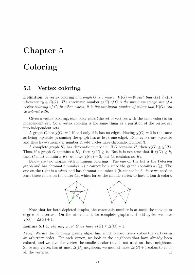
Below are two graphs with minimum colorings. The one on the left is the Petersengraph and has chromatic number 3 (it cannot be 2 since the graph contains a C5). Theone on the right is a wheel and has chromatic number 4 (it cannot be 3, since we need atleast three colors on the outer C5, which forces the middle vertex to have a fourth color).

Note that for both depicted graphs, the chromatic number is at most the maximumdegree of a vertex. On the other hand, for complete graphs and odd cycles we haveχ(G) = ∆(G) + 1.

Lemma 5.1.1. For any graph G we have χ(G) ≤ ∆(G) + 1.

Proof. We use the following greedy algorithm, which consecutively colors the vertices inan arbitrary order. For each vertex, we look at the neighbors that have already beencolored, and we give the vertex the smallest color that is not used on those neighbors.Since any vertex has at most ∆(G) neighbors, we need at most ∆(G) + 1 colors to colorall the vertices.

21

The greedy algorithm can be refined somewhat, by choosing the ordering in a certainway, so that it does better on some graphs. However, the problem of determining thechromatic number of a graph is NP-hard, so we do not know any fast algorithm thatalways works. We do have an algorithm for determining whether or not a graph haschromatic number two, since we have seen an algorithm for determining if a graph isbipartite.

As mentioned, complete graphs and odd cycles have χ(G) = ∆(G)+1, so the inequalityin Lemma 5.1.1 cannot be improved in general. In fact, complete graphs and odd cyclesare the only connected graphs that attain equality, but we will not prove this until later.For now, we prove a weaker statement by choosing a specific ordering for the greedyalgorithm.

Lemma 5.1.2. If a connected graph G has χ(G) = ∆(G) + 1, then G is regular.

Proof. We show that if G is not regular, then we can choose an ordering of the verticesso that the greedy algorithm from the proof of Lemma 5.1.1 needs only ∆(G) colors. Setn = |V (G)|. Assume G is not regular, so there is a vertex of degree at most ∆(G) − 1,which we label xn.

We grow a spanning tree from xn: Starting with T consisting only of the vertexxn, we repeatedly add to T an edge from ∂(T ). Since G is connected, this will indeedterminate with a spanning tree. While doing this, we label the vertices xn−1, xn−2, . . . , x1

in decreasing order as we add them. We claim that the resulting sequence x1, . . . , xn hasthe property that each vertex has at most ∆(G) − 1 neighbors in the sequence beforeit. Indeed, any xi with i < n has a unique path to xn in the tree, and by constructionthe labels on the vertices of this path increase from xi to xn. Thus xi has at least oneneighbor xj with j > i. The claim also holds for xn, because we chose xn to have degreeat most ∆(G)− 1.

We apply the greedy algorithm from the proof of Lemma 5.1.1, with the vertices inthe ordering x1, . . . , xn. When we are about to color xi, at most ∆(G)−1 of its neighborsare already colored, so ∆(G) colors suffice.

5.2 Edge coloring

Definition. An edge coloring of a graph G is a map c : E(G)→ N such that c(e) 6= c(e′)whenever e, e′ are distinct edges that share a vertex. The edge-chromatic number χe(G) ofG is the minimum image size of an edge coloring of G; in other words, it is the minimumnumber of colors that E(G) can be colored with.

Each color class in an edge coloring is a matching, so an edge coloring is partition ofthe graph into matchings.

An even cycle has edge-chromatic number 2 and an odd cycle has edge-chromaticnumber 3. The picture on the left below is an edge coloring of the Petersen graph withfour colors. We now prove that four is the minimum number (the picture on the rightillustrates the proof). Suppose we could color it with three colors. The outside C5 needsthree colors, and there must be three consecutive vertices on that C5 that are incidentwith only two colors (here red and blue). Then the third edge of each of those threevertices must have the third color (here green). But then this third color cannot be usedon the inside C5.

22

Lemma 5.2.1. For any graph G with at least one edge we have ∆(G) ≤ χe(G) ≤ 2∆(G)−1.

Proof. There must a vertex of degree ∆(G), and an edge coloring must give a differentcolor to each of the ∆(G) edges at that vertex. This implies χe(G) ≥ ∆(G).

The upper bound follows by a greedy algorithm just like that in the proof of Lemma5.1.1. Take an arbitrary ordering of the edges, and consecutively color each edge with thesmallest color that is not yet used on the colored edges that it shares a vertex with. Sincean edge shares a vertex with at most 2(∆(G)− 1) edges, it follows that 2∆(G)− 1 colorssuffice.

Unlike for vertex coloring, the greedy algorithm for edge coloring can be significantlyimproved on. This is shown in the proof of the following theorem, which tells us thatany graph G has edge-chromatic number either ∆(G) or ∆(G) + 1. Both are possible,since even cycles have χe(G) = ∆(G) and odd cycles have χe(G) = ∆(G) + 1. However,this algorithm still does not always give the exact number, and in fact it is NP-hard todetermine which of the two values is the edge-chromatic number of a given graph.

Theorem 5.2.2 (Vizing). For any graph G we have χe(G) ≤ ∆(G) + 1.

Proof. We use induction on the number of edges; the statement clearly holds for a graphwithout edges. Given an edge xy ∈ E(G), we describe an algorithm that, given an edgecoloring of G − xy with at most ∆(G) + 1 colors, produces an edge coloring of G withthe same number of colors. To find a color for xy, the algorithm may have to change thecolors of other edges, so it is not a greedy algorithm.

We first give some ad hoc definitions.

• If no edge incident with vertex v has color c, then we say that c is free at v, or thatv is c-free.

• Given two colors c, d, a cd-path is a path in G−xy whose edges are colored c and d.If a cd-path is maximal, then we can invert it by switching the colors c and d alongthe path. The result will still be an edge coloring, because if there were a conflict,then the path would not be maximal.

• A fan consists of a vertex x, a sequence y0, . . . , yk of distinct neighbors of x, and asequence c1, . . . , ck of distinct colors, such that xy0 is uncolored, and for 1 ≤ i ≤ k,xyi has color ci and yi−1 is ci-free. We can rotate a fan by recoloring edge xyi−1

with color ci for i = 1, . . . , k, and leaving xyk uncolored; the result is still an edgecoloring (except for xyk).

Given an edge coloring of G − xy with ∆(G) + 1 colors, we begin by constructing afan based at x with y0 = y as follows. Since we have ∆(G) + 1 colors and y0 has degreeat most ∆(G), there is a color c1 that is free at y0. If there is an edge incident to x withcolor c1, then we label its other endpoint y1. We continue like this: We pick a color ci+1

23

that is free at yi, and if possible we pick a ci+1-colored edge xyi+1 that is not yet in thefan. This terminates when we have a vertex yk that is c-free for some color c, but thereis no new edge incident to x with color c.

Given this fan, there is a color c that is free at yk, and there is a color d that is freeat x. We take a maximal cd-alternating path containing x. Such a path either consists ofx, or it starts at x with a c-edge, possibly followed by a d-edge, etc. We invert the path,which gives a new edge coloring.

After this inversion x is c-free. We claim that for some 1 ≤ ` ≤ k, y` is c-free, andx, y1, . . . , y` still forms a fan. If the alternating path was just x, and the inversion didnothing, then we can take the whole fan. Otherwise, the path started with some c-edgexyi+1, and yi must have been c-free before the inversion; in other words, ci = c. If thepath did not contain yi, then x, y1, . . . , yi is still a fan. Indeed, the colors c1, . . . , ck aredistinct, so for j ≤ i the inversion did not affect the fact that xyj has color cj or the factthat yj−1 is cj-free. If the path did somehow reach yi, then the inversion made it d-free,and it colored xyi+1 with d. In this case, x, y1, . . . , yk is still a fan, with the only changewithin the fan being that ci is replaced with d.

In all cases we have a fan x, y1, . . . , y` in which x and y` are c-free. Now we can rotatethe fan, so that the uncolored edge xy0 = xy becomes colored, and xy` becomes uncolored.Then we can color xy` with c.

5.3 Line graphs

Definition. The line graph of a graph G is the graph L(G) with vertex set V (L(G)) =E(G), and with e, e′ ∈ V (L(G)) adjacent if e and e′ share a vertex in G.

Line graphs explain some similarities that you may have noticed, between edge coloringand vertex coloring, and matchings and independent sets. From the definitions it shouldbe clear that

χe(G) = χ(L(G)),

and similarly thatm(G) = α(L(G)).

The cycle of a line graph is the cycle itself, which explains why the chromatic numberof a cycle equals its edge-chromatic number (if that needed any explanation).

We have ∆(L(G)) ≤ 2(∆(G) − 1), since if two vertices of degree ∆(G) are adjacent,then their edge corresponds to a vertex of degree 2(∆(G)−1) in the line graph. Thus theupper bound χe(G) ≤ 2∆(G)−1 actually follows from the upper bound χ(G) ≤ ∆(G)+1(and indeed, the proofs were essentially the same).

Here is another example where this connection is useful.

Lemma 5.3.1. For any graph G we have χ(G) ≥ |V (G)|α(G)

and χe(G) ≥ |E(G)|m(G)

.

Proof. First we prove that χ(G)α(G) ≥ |V (G)|. Given a coloring with χ(G) colors, thecolor classes (label them S1, . . . , Sχ(G)) are independent sets, and thus have size at mostα(G). Hence we have

|V (G)| =χ(G)∑i=1

|Si| ≤χ(G)∑i=1

α(G) = χ(G)α(G).

The second inequality follows directly by applying the first one to the line graph of G.

24

Not every graph is a line graph. Suppose for instance that the following graph H isa line graph L(G). The pair of vertices of H connected by the horizontal edge wouldcorrespond to a path xyz in G. The edges in G corresponding to the top and bottomvertex of H have to touch both edges of the path xyz, so one should be incident onlywith y and one should connect x and z. But then the edge of G corresponding to therightmost vertex of H cannot touch the edge xz without touching xy or yz, which is acontradiction.

We can now look back at the algorithmic facts that we have seen. In general, there is nogood algorithm for finding independent sets. But, for graphs that are line graphs, findingan independent set in L(G) is equivalent to finding a matching in G, for which there isa good algorithm. Similarly, there is no good algorithm for determining the chromaticnumber of a graph, and the greedy algorithm is basically the best we have. But, forline graphs, determining the chromatic number of L(G) is the same as determining theedge-chromatic number of G. For that there is a non-greedy algorithm which does a lotbetter, since it gives an edge coloring of G (and thus a vertex coloring of L(G)) that iseither minimal or has one color too much.

25

Chapter 6

Hamilton cycles

6.1 Girth and circumference

Definition. The girth gir(G) of a graph G is the length of the shortest cycle containedin G. The circumference circ(G) is the length of the longest cycle contained in G.

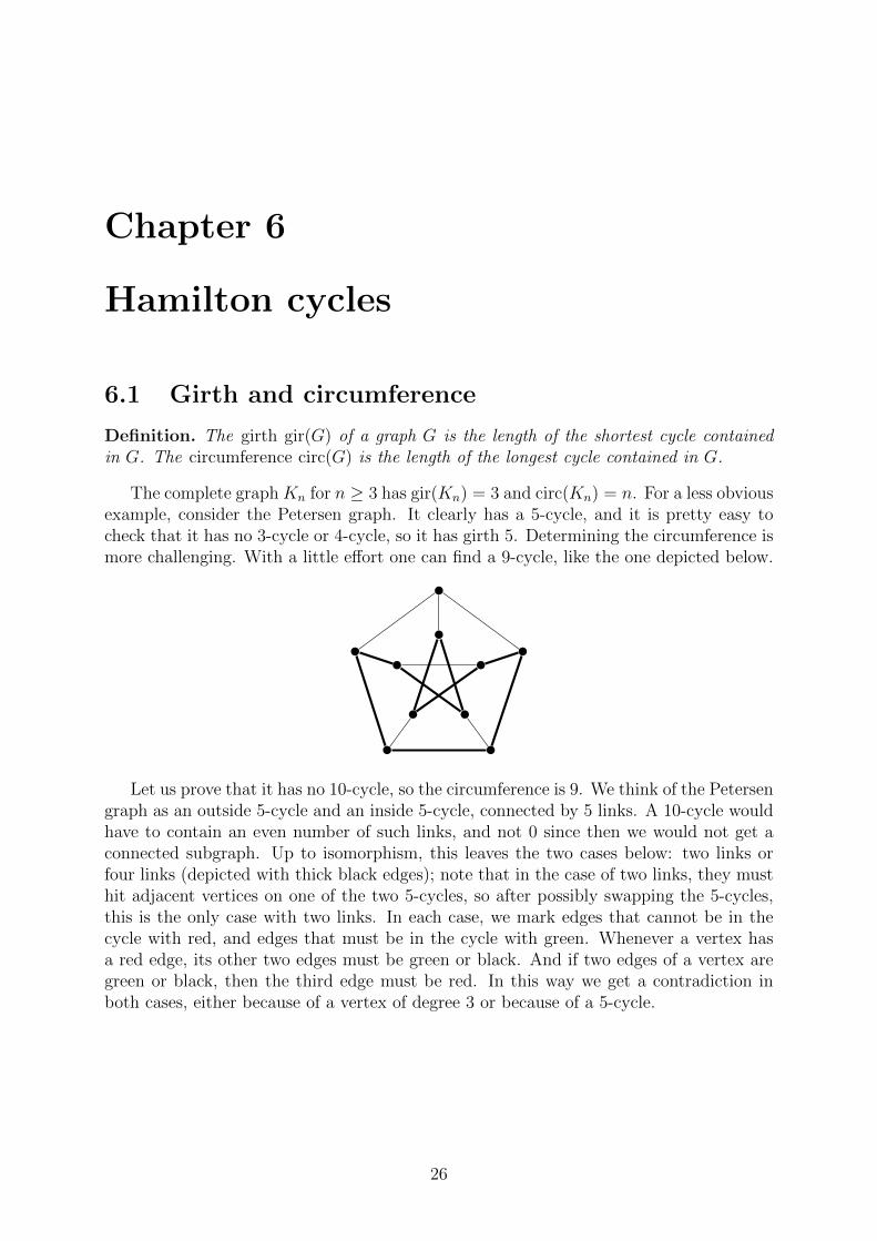
The complete graph Kn for n ≥ 3 has gir(Kn) = 3 and circ(Kn) = n. For a less obviousexample, consider the Petersen graph. It clearly has a 5-cycle, and it is pretty easy tocheck that it has no 3-cycle or 4-cycle, so it has girth 5. Determining the circumference ismore challenging. With a little effort one can find a 9-cycle, like the one depicted below.

Let us prove that it has no 10-cycle, so the circumference is 9. We think of the Petersengraph as an outside 5-cycle and an inside 5-cycle, connected by 5 links. A 10-cycle wouldhave to contain an even number of such links, and not 0 since then we would not get aconnected subgraph. Up to isomorphism, this leaves the two cases below: two links orfour links (depicted with thick black edges); note that in the case of two links, they musthit adjacent vertices on one of the two 5-cycles, so after possibly swapping the 5-cycles,this is the only case with two links. In each case, we mark edges that cannot be in thecycle with red, and edges that must be in the cycle with green. Whenever a vertex hasa red edge, its other two edges must be green or black. And if two edges of a vertex aregreen or black, then the third edge must be red. In this way we get a contradiction inboth cases, either because of a vertex of degree 3 or because of a 5-cycle.

26

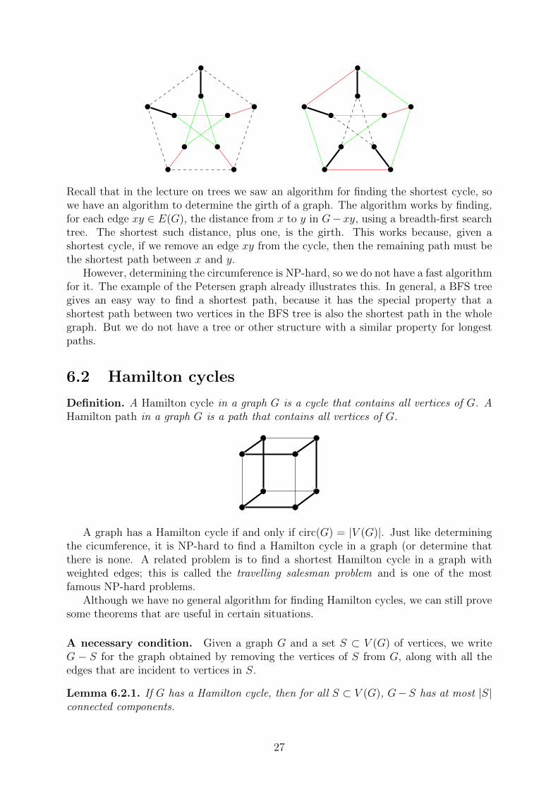
Recall that in the lecture on trees we saw an algorithm for finding the shortest cycle, sowe have an algorithm to determine the girth of a graph. The algorithm works by finding,for each edge xy ∈ E(G), the distance from x to y in G− xy, using a breadth-first searchtree. The shortest such distance, plus one, is the girth. This works because, given ashortest cycle, if we remove an edge xy from the cycle, then the remaining path must bethe shortest path between x and y.

However, determining the circumference is NP-hard, so we do not have a fast algorithmfor it. The example of the Petersen graph already illustrates this. In general, a BFS treegives an easy way to find a shortest path, because it has the special property that ashortest path between two vertices in the BFS tree is also the shortest path in the wholegraph. But we do not have a tree or other structure with a similar property for longestpaths.

6.2 Hamilton cycles

Definition. A Hamilton cycle in a graph G is a cycle that contains all vertices of G. AHamilton path in a graph G is a path that contains all vertices of G.

A graph has a Hamilton cycle if and only if circ(G) = |V (G)|. Just like determiningthe cicumference, it is NP-hard to find a Hamilton cycle in a graph (or determine thatthere is none. A related problem is to find a shortest Hamilton cycle in a graph withweighted edges; this is called the travelling salesman problem and is one of the mostfamous NP-hard problems.

Although we have no general algorithm for finding Hamilton cycles, we can still provesome theorems that are useful in certain situations.

A necessary condition. Given a graph G and a set S ⊂ V (G) of vertices, we writeG − S for the graph obtained by removing the vertices of S from G, along with all theedges that are incident to vertices in S.

Lemma 6.2.1. If G has a Hamilton cycle, then for all S ⊂ V (G), G−S has at most |S|connected components.

27

Proof. The Hamilton cycle must visit all the components of G− S (viewed as subgraphsof G), and to get from one component to another the cycle must pass through a vertexof S. Thus every component is connected to S by two edges of the cycle (and possiblyby other edges not in the cycle). Since every vertex is incident to two edges of the cycle,we have that twice the number of components is at most twice the number of vertices ofS.

This lemma can be useful to show that a graph does not have a Hamilton cycle. Forexample, if in the left-hand graph G below we let S consist of the middle two vertices, thenG − S has three connected components, so by Lemma 6.2.1 the graph has no Hamiltoncycle.

On the other hand, one can check that the right-hand graph H satisfies the conditionthat for all S ⊂ V (H), H − S has at most |S| components. Nevertheless, the graph hasno Hamilton cycle. To see this, observe that for the vertices of degree 2, both incidentedges would have to be in the cycle; but then the middle vertex would be incident to threeedges of the cycle, which is impossible.

6.3 Sufficient conditions

Next we prove two sufficient conditions for a graph to have a Hamilton cycle. First weshow that a graph with many edges must have a Hamilton cycle. However, note that thisbound is suprisingly weak, because a graph with this many edges is almost complete. Inthe proof the following definition will be convenient.

Definition. The complement of a graph G is the graph G with vertex set V (G) = V (G)and edge set E(G) = {xy : x, y ∈ V (G), xy 6∈ E(G)}.

Theorem 6.3.1. If G is a graph with |E(G)| >(|V (G)|−1

2

)+ 1, then G has a Hamilton

cycle.

Proof. Set n = |V (G)|. The statement is clearly true for n = 1, 2, 3, so we assume n > 3.Note that

(n−1

2

)+ 1 =

(n2

)− (n − 2). Thus the condition of the theorem means that

|E(G)| < n − 2. Thus∑dG(v) = 2(n − 2) < 2n, which implies that there must be a

vertex v such that dG(v) ≤ 1. Then we have dG(v) ≥ n− 2. We remove the vertex v fromG, and we will apply induction to G− v. We distinguish the two cases d(v) = n− 2 andd(v) = n− 1.

Suppose d(v) = n− 2. Then

|E(G−v)| = |E(G)|−(n−2) >

(n− 1

2

)+1−(n−2) =

(n− 2

2

)+1 =

(|V (G− v)| − 1

2

)+1.

28

Hence, by induction, the graph G − v has a Hamilton cycle C. Since d(v) = n − 2 andn > 3, v must have two neighbors u,w that are adjacent on C. Then we can remove uwfrom C and replace it by uv and vw, which results in a Hamilton cycle for G.

Suppose d(v) = n − 1. In this case we only have |E(G − v)| >(|V (G−v)|−1

2

), so we

cannot apply induction right away. If G−v is complete, then G−v has a Hamilton cycle,and we can add v as in the previous case. Otherwise, we can add an arbitrary edge e toG−v, and apply induction to find a Hamilton cycle C in G−v+ e. If C does not containe, then we can again add v as in the previous case. If C does contain e, then removinge from C gives a “Hamilton path” P in G− v. Since d(v) = n− 1, v is connected to allvertices of G − v, and in particular to the endpoints u,w of P . Then adding uv and vwto P gives a Hamilton cycle of G.

The statement in Theorem 6.3.1 cannot be improved, in the sense that a weaker boundon |E(G)| does not imply a Hamilton cycle. Take for instance the graph G consisting ofKn−1 and a single vertex connected to a single vertex of Kn−1. This graph has |E(G)| =(n−1

2

)+ 1, but it has no Hamilton cycle, since it has a vertex of degree 1.

As said, the condition in Theorem 6.3.1 is somewhat weak in the sense that manygraphs that have a Hamilton cycle do not satisfy the condition. The following sufficientcondition does better by looking at the minimum degree instead of the total number ofedges. Its proof is a typical extremal argument that we have seen before, for instance inthe proof of a lemma in Lecture 1, which said that a graph must have a cycle of lengthδ(G) + 1. But note that that lemma by itself is not strong enough to imply a Hamiltoncycle.

Theorem 6.3.2 (Dirac). Let G be a graph with |V (G)| ≥ 3. If δ(G) ≥ 12|V (G)|, then G

has a Hamilton cycle.

Proof. First observe that G must be connected, since otherwise each connected componentwould contain at least δ(G) + 1 > 1

2|V (G)| vertices, which is impossible.

Take a longest path P = x1x2 · · ·xk in G. By maximality, all neighbors of x1 and xkare on the path. Thus δ(G) ≥ 1

2|V (G)| gives the following two inequalities:

|{xi : 1 ≤ i ≤ k − 1, xixk ∈ E(G)}| ≥ 1

2|V (G)|,

|{xi : 1 ≤ i ≤ k − 1, xi+1x1 ∈ E(G)}| ≥ 1

2|V (G)|.

In other words, we have two subsets of size at least 12|V (G)| that are contained in the

set {x1, . . . , xk−1}, which has k − 1 < |V (G)| elements. It follows that the two subsetsshare an element xi, which means that we have xixk ∈ E(G) and xi+1x1 ∈ E(G). ThenC = xi · · ·x1xi+1 · · ·xkxi is a cycle.

In fact, C is a Hamilton cycle. Indeed, suppose there is a vertex u not in C. SinceG is connected, there is a path from u to (say) x1. There is a vertex v on this path thatis not on C but that is adjacent to some xj. Then there is a path that goes from v toxj, then all around the cycle C to a neighbor of xj. This path contains k + 1 vertices,contradicting the maximality of P .

This theorem is again best possible, in the sense that a weaker bound on the minimumdegree would not imply a Hamilton cycle. Take for instance the graph G consisting of twocopies of Kk sharing a single vertex. This graph has n = 2k − 1 vertices and minimumdegree δ(G) = k − 1 = 1

2|V (G)| − 1

2, but no Hamilton cycle.

29

Chapter 7

2-connected graphs

7.1 2-connectedness

In this lecture we look at graphs that are “more connected” than other connected graphs.Recall that if G is a graph and x ∈ V (G), then G − v is the graph with vertex setV (G)\{x} and edge set E(G)\{e : x ∈ e}.

Definition. A graph G is 2-connected if |V (G)| > 2 and for every x ∈ V (G) the graphG− x is connected.

A vertex v ∈ V (G) such that G−v is disconnected is called a cut-vertex ; a graph withat least three vertices is thus 2-connected if it has no cut-vertices. If G is 2-connected,then δ(G) ≥ 2, since if a vertex has degree 1 (in a connected graph with more than twovertices), then its neighbor is a cut-vertex.

Cycles Cn are 2-connected, as are complete graphs Kn for n > 2. Trees are not 2-connected: Removing a vertex that is not a leaf disconnects the graph, since otherwisethere would be a path connecting its neighbors, which would give a cycle in the tree.

One can similarly define a cut-edge to be an edge e ∈ E(G) such that G − e isdisconnected, and a graph to be 2-edge-connected if it has no cut-edges. However, in thislecture we will focus on vertex connectivity.

Our first theorem gives a constructive characterization of 2-connected graphs. This isuseful for visualizing such graphs, and can be used in induction proofs.

Definition. An ear decomposition of a graph G consists of a cycle C and a sequenceof paths P1, . . . , Pk such that G can be constructed by starting with C and consecutivelyattaching the paths Pi by their endpoints.

Theorem 7.1.1. A graph G is 2-connected if and only if it has an ear decomposition.

Proof. Suppose G has an ear decomposition. The cycle that the decomposition startswith is 2-connected. For any 2-connected graph H, attaching a path P by its endpointsgives a 2-connected graph: If we remove an internal vertex from P , each of the othervertices of P is connected to one of its endpoints, and thus to all of H; if we remove avertex x from H (which may be an endpoint of P ), then H − x is still connected, and Pis still connected to H via at least one of its endpoints. It follows that a graph that hasan ear decomposition is 2-connected.

Assume that G is 2-connected. Then it is not a tree, so it has a cycle. We will showthat we can build an ear decomposition starting with any cycle C.

30

Let H be any 2-connected subgraph of G with V (H) 6= V (G). Let x be a vertex inV (G)\V (H). Since G is connected, there is a path from x to any vertex in H, and thispath contains a vertex y 6∈ V (H) that is adjacent to a vertex z ∈ V (H). Since G is2-connected, G− z is connected, so there is a path in G− z from y to a vertex in H. Takethe part of that path that goes from y to the first vertex of the path that is in H (whichis not z). This subpath, combined with yz, is an “ear” that we can attach to H.

Therefore, starting with any cycle C, we can find such an ear and attach it, whichgives a larger 2-connected subgraph, and we can continue like this until there are novertices left. At that point any remaining edge is an ear, so we can add the remainingedges one-by-one.

7.2 Whitney’s Theorem

Recall that a graph is connected if there is a path between any two vertices. Thus itwould have made sense to define “2-connected” as any two vertices being connected bytwo paths. This would have been less convenient than the definition based on removalthat we gave above. Nevertheless, the next theorem shows that the result would basicallybe the same, if we require that the two paths share no vertices besides their endpoints.We call two paths internally disjoint if they share no vertices other than (possibly) theirendpoints.

Theorem 7.2.1 (Whitney). Let G be a graph with |V (G)| ≥ 3. Then G is 2-connectedif and only if for any distinct x, y ∈ V (G) there are two internally disjoint paths from xto y in G.

Proof. First we show that if every two vertices x, y ∈ V (G) are connected by two internallydisjoint paths, then G − z is connected for any z ∈ V (G), so G is 2-connected. Fixz ∈ V (G), and consider any two other vertices x, y ∈ V (G). There are two internallydisjoint paths from x to y, so z lies on at most one of these, and removing z breaks atmost one of the paths. Hence in G − z there is still a path between x and y. Since thisholds for any x, y ∈ V (G− z), G− z is connected.

Now assume that G is 2-connected and let x, y ∈ V (G). We use induction on thedistance d(x, y) to prove that there are two internally disjoint paths from x to y. Whend(x, y) = 1, the edge xy is one path. The fact that G−x and G−y are connected impliesthat G − xy is connected, so there is a path from x to y that does not contain xy, andthis is our second path.

Let d(x, y) = k > 1. Then there is a path from x to y of length k. Let z be the lastvertex before y on this path, so we have d(x, z) = k − 1. By induction, there are twointernally disjoint paths P1, P2 from x to z. Since G − z is connected, there is a pathQ from x to y in G that does not contain z. If Q does not intersect P1 or P2, then wehave two internally disjoint paths from x to y: Q, and P1 followed by zy. Suppose thatQ intersects P1 or P2 (possible more than once, and possibly both). Create one path bystarting from y, following Q until it first intersects P1 or P2, and then following that pathto x; note that this path avoids z. Create another path by combining the other one of P1

and P2 with zy. This gives two internally disjoint paths from x to y.

Corollary 7.2.2. A graph G is 2-connected if and only if for every two vertices x, y ∈V (G) there is a cycle in G that contains x and y.

31

Note that in a 2-connected graph we cannot guarantee that any three vertices lie on acycle. Take for instance K2,3, which is 2-connected. The three vertices on the larger sideare not on any cycle, because a cycle in a bipartite graph has the same number of verticesfrom both sides.

In the next lecture we will generalize 2-connectedness to k-connectedness, and we willsee generalizations of Theorem 7.2.1 and Corollary 7.2.2.

7.3 3-connectedness and Brooks’s Theorem

Definition. A graph G is 3-connected if |V (G)| > 3 and for all x, y ∈ V (G) the graphG− x− y is connected.

In this section we will use the notion of 3-connectedness to prove an important theoremon vertex coloring. Our proof does not actually use any theorems about 3-connectedness,but the property is exactly what we need to distinguish between the two main cases inthe proof. This is why we postponed this theorem to the current lecture.

Recall that for any graph G we have χ(G) ≤ ∆(G) + 1. We already saw a proofthat when equality holds, G must be a regular graph. Brooks’s Theorem refines thatstatement.

Theorem 7.3.1 (Brooks). Let G be a connected graph. If χ(G) = ∆(G) + 1, then G isa complete graph or an odd cycle.

Proof. Set ∆ = ∆(G). In Lecture 5 we saw that if χ(G) = ∆ + 1, then G must be ∆-regular. The proof worked as follows: If G has a vertex x of degree less than ∆, then wecan order the vertices using a spanning tree, in such a way that every vertex has a neighborthat comes later in the order, except for x, which comes last; the greedy algorithm is thenable to color all vertices with ∆ colors. We will use that idea again.

First note that if ∆ = 0, 1, the statement is trivial, and if ∆ = 2 then it is easy to seethat G must be an odd cycle. So we can assume that ∆ ≥ 3. We will distinguish betweenthe case where G is 3-connected and the case where G is not 3-connected.

Suppose that G is 3-connected. We can assume that there are two vertices x1, x2 ∈V (G) such that d(x1, x2) = 2, since otherwise G is complete and we are done. Thus x1

and x2 are not adjacent, but there is a vertex xn that is adjacent to both. Since G is3-connected, G−x1−x2 is connected. We build a tree in G with xn as root, by repeatedlyadding vertices xn−1, . . . , x3 from G − x1 − x2, with each xi having at least one edge toone of the previous vertices.

Now we apply the greedy algorithm with the vertex order x1, x2, . . . , xn to color Gwith at most ∆ colors. Since x1 and x2 are not adjacent, they get the same color. Sinceeach of the vertices x3, . . . , xn−1 has ∆ neighbors, at least one of which is uncolored whenthe algorithm reaches the vertex, each of these vertices can be colored with one of the∆ colors. Finally, when the algorithm reaches xn, all its ∆ neighbors are colored, but x1

and x2 are neighbors of xn with the same color, so there is a color left to color xn with.This shows that χ(G) ≤ ∆(G) if G is 3-connected and not complete.

Now suppose that G is not 3-connected. In this case there are x, y ∈ V (G)such that G − x − y is not connected. We can take subgraphs G1 and G2 such thatV (G1) ∩ V (G2) = {x, y}, E(G1) ∪ E(G2) = E(G), and there are no edges between

32

V (G1)\{x, y} and V (G2)\{x, y}. Specifically, let G1 be one component of G − x − ycombined with x, y and all the edges with both endpoints in this set; let G2 be the unionof the remaining components, combined with x, y and all edges with both endpoints inthis set.

Since x and y must have edges in both G1 and G2, these graphs are not regular, socan be ∆-colored. If both can be colored with x, y having the same color, or both canbe colored with x, y having different colors, then we can combine the two colorings into a∆-coloring of G. In particular, if x and y are adjacent, then both colorings give x and ydifferent colors, so can be combined. Thus we can assume that x and y are not adjacent.

The remaining possibility is that every ∆-coloring of G1 gives x, y the same color,and every ∆-coloring of G2 gives x, y different colors (or vice versa). If a ∆-coloring ofG1 is forced to give x, y the same color, then it must be because dG1(x) = ∆ − 1 anddG1(y) = ∆ − 1. Indeed, if one of these degrees were lower, then we would have analternative color for one of the two vertices. But then dG2(x) = 1 and dG2(y) = 1, so since∆ ≥ 3 and x and y are not adjacent, it is not possible that a ∆-coloring of G2 is forcedto give x, y different colors. This is because only one color is blocked at each of x and y,and at least two colors are available at each, so there is one color that can be given toboth. This is a contradiction that finishes the proof.

33

Chapter 8

k-connected graphs

8.1 Menger’s Theorem

In this lecture we generalize our results from the previous lecture, from 2-connected graphsto k-connected graphs. We first prove the key tool behind these generalizations, which isMenger’s Theorem. Its proof is relatively difficult and requires a few ad hoc definitions.

Given two vertex sets A,B ⊂ V (G), we call a path an AB-path if one endpoint is inA, the other endpoint is in B, and no other vertex on the path is in A or B. If x ∈ A∩B,then we consider x itself to be an AB-path. We call a set S ⊂ V (G) such that everyAB-path intersects S an AB-separator.

Theorem 8.1.1 (Menger). Let G be a graph and A,B ⊂ V (G). The maximum numberof disjoint AB-paths equals the minimum size of a set S ⊂ V (G) such that every AB-pathcontains a vertex from S.

Proof. Let s be the minimum size of an AB-separator. Any set of disjoint AB-pathscontains at most s paths, since otherwise a separator of size s could not cut all the paths.We have to show that there exists a set of s disjoint AB-paths. We will prove this usinginduction on |E(G)|. When |E(G)| = 0, then the only minimum AB-separator is A ∩ Bitself, so we must have s = |A ∩B|, and the s vertices in A ∩B are disjoint AB-paths.

Assume |E(G)| ≥ 1 and let xy be any edge in E(G). We claim that if G does nothave s disjoint AB-paths, then G has an AB-separator S of size s that contains both xand y. We first show how to prove the theorem given this claim, and then we will provethe claim.

Consider the graph G − xy, in which S is still an AB-separator. Consider an AS-separator R in G−xy. Observe that every AB-path in G contains an AS-path in G−xy(this could fail if we did not have x, y ∈ S), so R is also an AB-separator in G, whichimplies |R| ≥ s. It follows that the minimum size of an AS-separator in G−xy is at leasts. By induction, this implies that G−xy has s disjoint AS-paths. By the same argumenton the other side, G−xy has s disjoint SB-paths. These AS-paths and SB-paths do notintersect outside S, since that would give an AB-path avoiding S. Since |S| = s, we canconnect the s AS-paths with the s SB-paths to obtain s disjoint AB-paths.

It remains to prove the claim that if G does not have s disjoint AB-paths, then G hasan AB-separator S of size s containing x and y. We contract xy to get the graph G/xy;this means that we remove xy and identify x and y to a vertex vxy. More precisely, weremove x, y, and all incident edges, add a new vertex vxy, and we connect vxy to everyvertex that was previously adjacent to x or y (or both). We modify A in the natural way:

34

If A does not contain x or y, then we let A′ be the same set in G/xy; if A does contain xor y (or both), then we set A′ = (A\{x, y}) ∪ {vxy}. We do the same with B to get B′.

An A′B′-path P in G/xy corresponds to one or more AB-paths in G: If vxy is not onP , then P is an AB-path in G; if vxy is on P , then there can be more than one way tomodify P to an AB-path in G. Conversely, an AB-path in G corresponds to an A′B′-pathin G/xy. Also note that disjoint A′B′-paths in G/xy correspond to disjoint AB-paths inG.

By assumption, G does not have s disjoint AB-paths, so G/xy does not have s disjointA′B′-paths. By induction (for the statement of the theorem, not just the claim), thisimplies that the minimum size of an A′B′-separator in G/xy is at most s − 1, so G/xyhas an A′B′-separator S ′ of size at most s − 1. We must have vxy ∈ S ′, since otherwiseS ′ would be an AB-separator in G that is smaller than the minimum (using the fact thatevery AB-path in G corresponds to an A′B′-path in G/xy). Set S = (S ′\{vxy}) ∪ {x, y}.It is an AB-separator in G of size s that contains x and y.

Corollary 8.1.2. Let G be a graph and x, y ∈ V (G) distinct vertices with xy 6∈ E(G).The maximum number of internally disjoint paths from x to y equals the minimum sizeof a set S ⊂ V (G)\{x, y} with the property that every path from x to y contains a vertexfrom S.

Proof. Apply Theorem 8.1.1 with A = N(x) and B = N(y). Note that adding x and yto an AB-path gives a path from x to y, but removing x and y from a path between xand y may not give an AB-path, because a path between x and y may pass through morethan one neighbor of x or y. Nevertheless, every path between x and y does contain asubpath that is an AB-path, so the maximum number of internally disjoint paths fromx to y equals the number of disjoint AB-paths. By Theorem 8.1.1, this maximum equalsthe minimum size of a set S ⊂ V (G) such that every AB-path intersects S. Any such setS also has the property that every path from x to y contains a vertex of S. It remains toshow that a minimum such set S does not contain x or y. If S contains x (say) and everyAB-path intersects S, then the same holds for S\{x}, since a path that goes from B toA via x contains a subpath from B to A that does not contain x, and that subpath mustcontain some other vertex of S.

8.2 k-connected graphs

Recall that for S ⊂ V (G), G−S is the subgraph obtained from G by removing the verticesof S and all edges incident with a vertex of S.

Definition. A graph is k-connected if |V (G)| > k and for every S ⊂ V (G) with |S| =k − 1 the graph G− S is connected.

Note that 1-connected is the same as connected, except (annoyingly) when |V (G)| = 1.

Theorem 8.2.1. A graph G is k-connected if and only if for any distinct x, y ∈ V (G)there are k internally disjoint paths from x to y in G.

Proof. If G contains k internally disjoint paths between any two vertices, then we musthave |V (G)| > k, and after removing k − 1 vertices, any two vertices are still connectedby one of the k paths, so G is k-connected.

35

Conversely, suppose that G is k-connected and contains two vertices x, y that are notconnected by k internally disjoint paths. If xy 6∈ E(G), then by Corollary 8.1.2 there arek − 1 vertices whose removal disconnects x from y, contradicting k-connectedness. Thuswe can assume that xy ∈ E(G).

By assumption, any set of internally disjoint paths connecting x and y has size at mostk−1. Moreover, any maximum such set includes the path xy, since otherwise we can addit. Thus G−xy has at most k−2 internally disjoint paths from x to y. By Corollary 8.1.2,there is a set S ⊂ V (G)\{x, y} of size k−2 such that every path from x to y intersects S.We have |S ∪ {x, y}| = k and |V (G)| > k, so there is a vertex z 6∈ S ∪ {x, y}. In G− xy,S must separate z from either x or y, since otherwise there would be a path from x to yavoiding S. Say that S separates z from x; then S ∪ {y} is a set of at most k− 1 verticesthat separates z from x in G, contradicting the k-connectedness of G.

Definition. The connectivity conn(G) of a graph G is the maximum k such that G isk-connected.

We have conn(Cn) = 2, conn(Kn) = n − 1 for n ≥ 3, and the connectivity of thePetersen graph is 3. Note that conn(G) ≤ δ(G), since if x is a vertex with d(x) = δ(G),then N(x) is a set of δ(G) vertices such that G−N(x) is not connected.

Finally, we prove the generalization of the fact from the last lecture that in a 2-connected graph every two vertices are contained in a cycle. The proof of that fact waseasy, since two internally disjoint paths between two vertices give a cycle containing thosetwo vertices. For more than two vertices, the proof is more interesting. We require thefollowing lemma.

Lemma 8.2.2. Let G be a k-connected graph. For every x ∈ V (G) and U ⊂ V (G) with|U | ≥ k, there are k paths from x to U that are disjoint aside from x, with each pathhaving exactly one vertex from U .

Proof. Add a vertex u that is adjacent to all the vertices in U ; the resulting graph isstill k-connected (this requires that |U | ≥ k). By Theorem 8.2.1, there are k internallydisjoint paths from x to u. Removing u from these paths gives paths from x to U that aredisjoint aside from x. If such a path contains more than one vertex of U , then it containsa subpath with exactly one vertex from U , which we can take instead.

Theorem 8.2.3 (Dirac). If a graph G is k-connected for k ≥ 2, then for every set K ofk vertices in G, there exists a cycle in G containing K.

Proof. We use induction on k. For k = 2, we saw a proof in the previous lecture; it alsofollows directly from the case k = 2 of Theorem 8.2.1. Assume k > 2 and pick any x ∈ K.By induction, G has a cycle C containing K\{x}. If x ∈ V (C), we are done, so we canassume that x 6∈ V (C).

Suppose that |V (C)| = k−1. By Lemma 8.2.2 and the fact that G is (k−1)-connected,there are k − 1 paths from x to C that are disjoint aside from x, each containing exactlyone vertex of C. We can use any two of the paths from x that end at adjacent verticesy, z ∈ V (C) to obtain a cycle containing x as well as K\{x}: Remove the edge yz fromC, and replace it by the path that goes from y to x and then from x to z. Since thesepaths were disjoint aside from x, and also contain no other vertices from C, this indeedgives a cycle.

Suppose that |V (C)| ≥ k. By Lemma 8.2.2 and the fact that G is k-connected, thereare k paths from x to C that are disjoint aside from x, each containing exactly one vertex

36

of C. The k − 1 vertices of K\{x} partition V (C) into k − 1 consecutive segments (foreach vertex of K\{x}, take that vertex and all the following ones, up to the one beforethe next vertex of K\{x}). By the pigeonhole principle, there must be a segment that isreached by two of the paths from x. Then as in the previous case these two paths can beused to obtain a cycle containing x as well as K\{x}.

37

Chapter 9

Planar graphs

9.1 Drawings of graphs

We have so far only considered abstract graphs, although we often used pictures to illus-trate the graph. In this lecture, we prove some facts about pictures of graphs and theirproperties. To set this on a firm footing, we give a formal definition of what we mean by“picture”, although in most of the lecture we will be less formal.

Definition. A drawing of a graph G consists of an injective map f : V (G)→ R2, and acurve Cxy (the image of an injective continuous map [0, 1] → R2) from x to y for everyxy ∈ E(G), such that if z 6= x, y then z 6∈ Cxy. A drawing is planar if the curves Cxy donot intersect each other except possibly at endpoints.

Definition. A graph is planar if it has a planar drawing.

For example, the graphs K4 and K2,3 are planar graphs.

Warning: Some proofs in this lecture will be not quite rigorous. This is mainlybecause arbitrary continuous curves can behave in unintuitive ways, which makes it hardto make intuitive arguments fully rigorous. Whenever an argument is not quite rigorous,we will point out why. In most cases, the arguments can be made rigorous using the JordanCurve Theorem, which states that a non-self-intersecting closed curve in R2 divides R2

into an inside and an outside, and any path between a point inside and a point outsidemust pass through the closed curve. Although this statement is very intuitive, proving itturns out to be quite hard. We will not try to prove it in this course, since it would takeus too far into topology and away from graph theory.

Definition. A face of a drawing D of a graph G is a maximal connected set in R2 afterthe vertices and edges of D are removed. We write FD(G) for the set of faces of D.

Every drawing has an outer face, which is the unique unbounded face in the comple-ment of the drawing. Note that although typically an edge lies in the boundary of twofaces, an edge can be in the boundary of a single face, which happens if and only if theedge is a cut-edge; this fact will create some complications later on.

9.2 Non-planar graph

To show that a graph is planar, we only have to supply a planar drawing. It is often alittle harder to show that a graph is not planar.

38

Proposition 9.2.1. The graph K5 is not planar.

Proof. The graph contains a K3, which can basically be drawn in only one way. If in adrawing the fourth vertex is inside this K3 and the fifth is outside, then the edge betweenthem must cross the K3, which means the drawing is not planar. If both vertices areinside the K3, then the three edges of one vertex divide the inside face into three faces.The other vertex must then be in one of these three faces, and one of its edges must crossthe boundary of this face. A similar argument applies when both vertices are outside theK3.

Note that to make this proof rigorous, we would need the Jordan Curve Theorem toshow that a drawing of a K3 has an inside and an outside, and that to connect a vertexinside to a vertex outside we would have to cross the K3.

Proposition 9.2.2. The graph K3,3 is not planar.

Proof. The graph contains a C6, and the remaining three edges connect opposite cornersof the C6 in a symmetric way. Two of these three edges would have to be both insideor outside the C6, and there one of them would create a closed curve that the other onewould have to cross. Again, this proof relies on the Jordan Curve Theorem.

If a graph H is a subgraph of a graph G and H is not planar, then G is also notplanar, since a planar drawing of G would give a planar drawing of H. A stronger versionof this is the following. Call a graph H ′ a subdivision of H if it can be obtained from Hby repeatedly replacing an edge xy by a path xzy for some new vertex z (informally, wesimply place the new vertex z somewhere on top of the edge xy, subdividing it into twoedges xz and zy). It is easy to see that a subdividion of H is planar if and only if H isplanar; the new vertices do not have any effect on whether ot not we can draw the graphwithout crossing edges.

Proposition 9.2.3. The Petersen graph is not planar.

Proof. It contains a subdivision of K3,3.

Amazingly, any non-planar graph can be shown to be non-planar by displaying asubdivision of K5 or K3,3 in that graph, and a planar graph can be shown to be planar byshowing that it does not contain such a subdivision. This is the content of the followingtheorem. Note that it states an equivalence between a topological statement (the graphhaving a planar drawing) and a combinatorial statement (the graph not containing acertain subdivision). The proof of this theorem is fairly hard and we will not include itin this course.

Theorem 9.2.4 (Kuratowski). A graph is planar if and only if it does not contain asubdivision of K5 or K3,3.

9.3 Euler’s formula

Theorem 9.3.1 (Euler). Let G be a connected planar graph and D a planar drawing ofG. Then

|V (G)| − |E(G)|+ |FD(G)| = 2.

39

Proof. We use induction on |E(G)|. Since G is connected, we have |E(G)| ≥ |V (G)| − 1,so we can start with the base case |E(G)| = |V (G)| − 1. In that case, G is a tree, so anyplanar drawing has only one face and we have |FD(G)| = 1. Then

|V (G)| − |E(G)|+ |FD(G)| = |V (G)| − (|V (G)| − 1) + 1 = 2.

Assume that |E(G)| > |V (G)|−1. Then G contains a cycle C. Pick an edge e ∈ E(C).The graph G − e is connected, and the drawing D directly gives a planar drawing D′

of G − e. Moreover, since e is in a cycle, it is not a cut-edge of G, so e is on theboundary of two different faces (one inside C, one outside C; here we use the JordanCurve Theorem). Removing e merges these two faces, and does not affect any other faces,so |FD′(G− e)| = |FD(G)| − 1. By induction, we have

|V (G− e)| − |E(G− e)|+ |FD′(G− e)| = 2.

Plugging in |V (G−e)| = |V (G)|, |E(G−e)| = |E(G)|−1, and |FD′(G−e)| = |FD(G)|−1gives Euler’s formula for G.

Note that Euler’s formula implies that for two planar drawings D1, D2 of a graph wehave |FD1(G)| = 2 − |V (G)| + |E(G)| = |FD2(G)|, so the number of faces in a planardrawing of a graph is independent of the drawing.

Proposition 9.3.2. Let G be a planar graph with |V (G)| ≥ 3. Then |E(G)| ≤ 3|V (G)|−6.

Proof. We can assume that G is maximally planar, i.e., that adding any edge to G wouldmake it non-planar. Indeed, given any planar graph, we can add edges until it is maximallyplanar; if the bound holds for the maximally planar graph, then it also holds for theoriginal graph. Then G is connected, every edge is in the boundary of two faces, andevery face has exactly three edges on its boundary, since if any of these properties did nothold, then we could add an edge.

Double counting the pairs (e, f), where the edge e is on the boundary of the face f ,gives us

2|E(G)| = 3|FD(G)|.

Plugging |FD(G)| = 23|E(G)| into Euler’s formula gives

2 = |V (G)| − |E(G)|+ 2

3|E(G)|,

which rearranges to |E(G)| = 3|V (G)| − 6. Since this equality holds for any maximallyplanar graph, the inequality |E(G)| ≤ 3|V (G)| − 6 holds for any planar graph.

It is possible to prove Proposition 9.3.2 in a more direct way, without assuming thegraph to be maximally planar. Basically, every edge bounds at most two faces, andevery face is bounded by at least three edges, so we should have 2|E(G)| ≥ 3|FD(G)|.Plugging that into Euler’s formula directly gives the inequality |E(G)| ≤ 3|V (G)| − 6 (toapply Euler’s formula, we need the graph to be connected, but we can apply it to eachconnected component, which leads to the same bound). However, it is not always truethat every edge bounds at most two faces and every face is bounded by at least threeedges; take for instance the path P2, which has one face bounded by two edges. For P2 wehave 2|E(G)| ≥ 3|FD(G)| anyway, but it is tricky to prove that this holds for all graphs.The step of making the graph maximally planar is a convenient way around this.

40

Proposition 9.3.2 gives us a quick proof that K5 is not planar:

|E(K5)| =(

5

2

)= 10 > 9 = 3 · 5− 6 = 3|V (K5)| − 6.

This does not quite work for K3,3 or the Petersen graph, but their non-planarity can alsobe proved using Euler’s formula (see Problem Set 9 for K3,3).

Corollary 9.3.3. If G is planar, then it has a vertex of degree at most five.

Proof. Combining Proposition 9.3.2 with the degree formula from the first lecture gives∑v∈V (G)

d(v) = 2|E(G)| ≤ 6|V (G)| − 12.

This implies that the average degree of a vertex is strictly less than six, so there must bea vertex with degree at most five.

9.4 Coloring planar graphs

Theorem 9.4.1 (Five Color Theorem). If G is planar then χ(G) ≤ 5.

Proof. Fix a planar drawing of G. We use induction on |V (G)|. The statement is obviousfor |V (G)| ≤ 5. By Corollary 9.3.3, there is a vertex v ∈ V (G) of degree at most five. Byinduction, we can color G − v with five colors. If this coloring uses at most four colorson N(v), then we can color v with the fifth color and we are done. Thus we can assumethat v has five neighbors x1, . . . , x5, and that xi has color i. We can also assume that theedges vx1, . . . , vx5 leave v in that order when we go around v in the clockwise direction(say).

We call a path in G an ij-path if all its vertices have color i or j.Suppose that there is no 13-path from x1 to x3. Let R be the set of vertices that are

reachable from x1 by a 13-path. By assumption, x3 is not in R. Then we can swap thecolors 1 and 3 for all the vertices in R. This gives a valid coloring, and it leaves x1 andx3 both colored with 3. Then we can color v with 1 and we are done.

Now suppose that there is a 13-path from x1 to x3; together with v this path formsa cycle C, all of whose vertices are colored with 1 or 3 (or uncolored in the case of v).Let S be the set of vertices reachable by 24-paths from x2. Then the cycle C separates Sfrom x4 (here we use the Jordan Curve Theorem), so x4 is not in S. Thus we can swapcolors 2 and 4 in S, and then color v with 2.

This theorem is actually not best possible. The famous Four Color Theorem statesthat for any planar graph we have χ(G) ≤ 4. However, the proof is extremely hard andhas only been completed using computers to check many cases.

41

Chapter 10

Extremal graph theory I

10.1 Extremal graph theory

Extremal graph theory is a wide area that studies the extremal values of graph parametersfor graphs with certain properties. We have seen various examples in this course; forinstance, we saw an upper bound for the number of edges in a graph without a Hamiltoncycle. In this lecture (and the next), we will focus on a specific subset of problems fromextremal graph theory, namely bounds on the number of edges of a graph not containinga fixed subgraph.

Definition. Let H be a graph. A graph G is H-free if G does not contain H. We writeexH(n) for the maximum number of edges in an H-free graph on n vertices. An extremalgraph for H is an H-free graph that has n vertices and exH(n) edges.

To give a simple example, consider H = . We claim that exH(n) = n− 1 for n ≥ 4.Indeed, if we pick one edge xy in an H-free graph, then every other edge must share avertex with it. If one edge contains x and another contains y, then they must form atriangle, and there can be no other edges. Otherwise, all edges contain the same endpointof e, which implies that there are at most n − 1 edges. This proof also shows that theonly extremal graph for H is the star K1,n−1.

Usually, we first look for an upper bound on exH(n), and then we try to find extremalgraphs matching that bound. Sometimes that will work perfectly and we can determineexH(n) exactly (see Section 10.2), while other times it turns out to be harder and we haveto settle for upper and lower bounds for exH(n) (see Section 3).

Compared to the previous lectures, extemal graph theory relies more often on formulasand inequalities. In this lecture we only need the following standard inequality.

Lemma 10.1.1 (Cauchy-Schwarz). Let x1, . . . , xk and y1, . . . , yk be real numbers. Then(k∑i=1

xiyi

)2

≤k∑i=1

x2i

k∑i=1

y2i .

Equality holds if and only if the vector (xi) is a multiple of the vector (yi).

We will mostly use the following corollary, which follows by setting yi = 1 for all i.

42

Corollary 10.1.2. If x1, . . . , xk are real numbers, then

k∑i=1

x2i ≥

1

k

(k∑i=1

xi

)2

.

Equality holds if and only if all xi are equal.

10.2 Triangles

Theorem 10.2.1 (Mantel). If G contains no triangle, then |E(G)| ≤ 14|V (G)|2.

Proof. Suppose G contains no triangle. Pick any xy ∈ E(G). Then x and y have nocommon neighbor, since otherwise we would get a triangle. Thus N(x) and N(y) aredisjoint subsets of V (G)\{x, y}, so we have

(d(x)− 1) + (d(y)− 1) ≤ |V (G)| − 2,

which impliesd(x) + d(y) ≤ |V (G)|.

Summing over all xy ∈ E(G), we get

|V (G)| · |E(G)| ≥∑

xy∈E(G)

(d(x) + d(y)) =∑

x∈V (G)

d(x)2.

The equality holds because in the sum on the left, a term d(x) occurs exactly d(x) times,once for each edge incident to x. Applying Cauchy-Schwarz, or more specifically Corollary10.1.2, and using

∑d(x) = 2|E(G)|, this gives

|V (G)| · |E(G)| ≥∑

x∈V (G)

d(x)2 ≥ 1

|V (G)|

∑x∈V (G)

d(x)

2

=4|E(G)|2

|V (G)|.

This proves the theorem.

Corollary 10.2.2. We have exK3(n) = bn2

4c, and the only extremal graph for K3 is

Kbn2c,dn

2e.

Proof. The number of edges is always an integer, so Theorem 10.2.1 gives exK3(n) ≤ bn2

4c.

The graph Kbn2c,dn

2e has no triangle and has⌊n

2

⌋·⌈n

2

⌉=

⌊n2

4

⌋edges, so we have exK3(n) = bn2

4c. To see that there is no other extremal graph (up to

isomorphism of course), we have to look back at the proof of Theorem 10.2.1.Let us assume that n is even1. To get an equality in the bound, we must first of all

have an equality in the application of Cauchy-Schwarz. By Corollary 10.1.2, this happens

1The odd case is similar, but slightly more annoying, because then the d(x) are almost equal but notquite. In the next lecture, we will see a more general proof that gives the uniqueness of the extremalgraph in a more pleasant way.

43

if and only if all d(x) are equal. Then we must have equality in d(x) + d(y) ≤ n, sod(x) = 1

2n for all x. Pick any vertex x. It has 1

2n neighbors, which form an independent

set B. Each vertex in B has 12n neighbors, which is an independent set A disjoint from

B. It now follows that every vertex of A is adjacent to every vertex of B, which meansthat we have a complete bipartite graph with parts of size |A| = |B| = 1

2n.

Just for fun, we give another proof of Theorem 10.2.1.

Alternative proof of Theorem 10.2.1. We use a technique called weight shifting. Let G bea graph without triangles. We begin with a weight w(x) = 1 on every vertex x ∈ V (G).We will maximize

S =∑

xy∈E(G)

w(x)w(y)

by moving the weights around, in such a way that the total weight stays the same (equal to|V (G)|), while S never decreases. When we start with every weight 1, we have S = |E(G)|.

Write W (x) = w(N(x)) for the total weight of the neighbors of a vertex. Let x, y ∈V (G) be two non-adjacent vertices with W (x) ≥ W (y). Then for any s ≥ 0 we have

(w(x) + s)W (x) + (w(y)− s)W (y) ≥ w(x)W (x) + w(y)W (y).

This means that we can shift any weight from y to x without decreasing S.In general, for any two non-adjacent vertices with nonzero weight, we can shift all the

weight of the one with smaller W to the one with larger W . When we do this repeatedly,we increase the number of vertices with weight 0 in each step. Therefore, after finitelymany steps we cannot make any further steps, which must be because all vertices withnonzero weight have become pairwise adjacent. But there is no triangle, so at this pointwe must have all the weight on (at most) two adjacent vertices x, y. The maximum valueof w(x)w(y), under the condition w(x) +w(y) = |V (G)|, occurs when w(x) and w(y) areequal, so

S ≤ 1

2|V (G)| · 1

2|V (G)| = 1

4|V (G)|2.

Note that 12|V (G)|may not be an integer, but the upper bound still holds. Observe that we

started with S = |E(G)|, and S did not decrease while shifting, so |E(G)| ≤ 14|V (G)|2.

10.3 Squares

Theorem 10.3.1 (Erdos). If G contains no K2,2, then |E(G)| ≤ |V (G)|3/2.

Proof. Suppose G has no K2,2. Set n = |V (G)| and e = |E(G)|. We will double count thenumber of copies of K1,2 = P2 in G; write M for this number. On the one hand, for anyvertex we get a K1,2 for every pair of incident edges, so

M =∑

x∈V (G)

(d(x)

2

).

Because there is no K2,2, there can be no two K1,2 with the same two endpoints. Inother words, for any pair x, y of vertices, there is at most one z such that x, y, z form aK1,2 with x, y as endpoints. This gives us

M ≤(n

2

).

44

Now we calculate. We have obtained(n

2

)≥M =

∑x∈V (G)

(d(x)

2

)=

1

2

∑d(x)2 − 1

2

∑d(x).

Applying Cauchy-Schwarz and∑d(x) = 2e gives

1

2

∑d(x)2 − 1

2

∑d(x) ≥ 1

2n

(∑d(x)

)2

− 1

2

∑d(x) =

2e2

n− e.

For convenience we use slightly rough bounds. The expression on the right can bebounded below by e2/n (unless e < n, in which case we are done anyway). The binomialcoefficient

(n2

)can be roughly bounded above by n2. Thus we have

n2 ≥ e2

n,

which gives e ≤ n3/2 and proves the theorem.

Note that we were a bit rough with the inequalities in the proof of Theorem 10.3.1. Inthe Problem Set you will prove a tighter upper bound of the form |E(G)| ≤ 1

2|V (G)|3/2 +

c|V (G)| for some constant c. We now prove a lower bound, which is also rough, but itshows that 3/2 is the right exponent. With some more effort, it can be shown that thebound from the Problem Set is almost exactly the value of exK2,2(n).

Corollary 10.3.2. We have

1

16n3/2 − n ≤ exK2,2(n) ≤ n3/2.

Proof. The upper bound is Theorem 10.3.1. To prove the lower bound, we construct aK2,2-free graph with at least 1

2n3/2 edges.

Let p be a prime and consider the finite field Fp. Let G be the graph with vertex setF2p, where (a, b) ∈ F2

p is adjacent to (x, y) ∈ F2p if ax+ by = 1. We could think of an edge

between (a, b) and (x, y) as representing the fact that the point (x, y) lies on the line withequation ax+ by = 1 (although this is a bit confusing because we are thinking of a vertexboth as a point and as a line). Note that the vertex (0, 0) is an isolated vertex.

This graph is K2,2-free. A quick way to see it is to think of two vertices (a, b) and(a′, b′) as two lines, and a common neighbor (x, y) as an intersection point of those lines.Then the fact that two lines have at most one intersection point (which is true in anyplane over any field) implies that (a, b) and (a′, b′) have at most one common neighbor,which means there is no K2,2. Alternatively, we can just argue that the two equationsax+ by = 1 and a′x+ b′y = 1 have at most one common solution.

We claim that every vertex (x, y) 6= (0, 0) has degree at least p − 1. If both x and yare nonzero, then for every a there is a b such that ax+ by = 1, namely b = y−1(1− ax).The p values of a give p solutions to ax+ by = 1, but we do not count (a, b) = (x, y) if itis a solution, so (x, y) has at least p− 1 neighbors. If one of x, y is zero, then one of a, bis determined and the other can take any value. This proves the claim.

The graph G has n = p2 vertices, and the number of edges satisfies

|E(G)| = 1

2

∑v∈V (G)

d(v) ≥ 1

2(p2 − 1)(p− 1) ≥ 1

2p3 − p2 =

1

2n3/2 − n.

45

This proves the lower bound (actually, a better one) for any n that happens to be asquare of a prime. By a result from number theory2, for any n there is a prime p between12

√n and

√n. Then we can take the graph with p2 vertices, and add isolated vertices

until we have exactly n vertices. The resulting graph is still K2,2-free and has at least12p3 − p2 ≥ 1

16n3/2 − n edges.

10.4 Trees

We have seen that exH(n) can be quadratic in n, and that it can behave as n3/2, sosubquadratic but superlinear. We now consider trees, and we will see that exH(n) canalso be linear. It is actually true that exH(n) is linear in n if and only if H is a tree (or aforest), but this is more difficult. Another fact is that for any rational number r between1 and 2, there is a graph H such that exH(n) grows like nr.

Theorem 10.4.1. Let T be any tree. If G does not contain T , then |E(G)| < (|E(T )| −1)|V (G)|.

We prove the theorem via two convenient lemmas.

Lemma 10.4.2. If T is a tree, and G is a graph with δ(G) ≥ |E(T )|, then G contains T .

Proof. We use induction on |E(T )|. The statement is obvious when |E(T )| = 1. Letx ∈ V (T ) be a leaf of T , and let y ∈ V (T ) be its neighbor in T . By induction, G containsa copy of T − x. There may be more than one possible embedding of T − x in G, butwe fix one particular embedding. We write y for the vertex of G that corresponds to thevertex y of T in this embedding.

Since dG(y) ≥ δ(G) ≥ |E(T )| ≥ |V (T )| − 1, and since T − x has at most |V (T )| − 2vertices other than y, there is a neighbor of y in G that is not in the embedding of T − x.Hence, we can label this neighbor x to get an embedding of T in G.

The next lemma states that any graph has a subgraph with reasonably large minimumdegree. Note that the minimum degree of the subgraph is more than half the averagedegree of G, since that average is (

∑d(x))/|V (G)| = 2|E(G)|/|V (G)|.

Lemma 10.4.3. Any graph G with at least one edge has a subgraph H with δ(H) > |E(G)||V (G)| .

Proof. We use induction on |V (G)|. When |V (G)| = 2, the statement is true, because thesingle edge K2 has δ(K2) > 1/2.

If δ(G) > |E(G)|/|V (G)|, then we can take H = G, so we can assume there is x ∈ V (G)with d(x) ≤ |E(G)|/|V (G)|. Consider G− x. By induction, it has a subgraph H with

δ(H) >|E(G− x)||V (G− x)|

≥|E(G)| − |E(G)|

|V (G)|

|V (G)| − 1=|E(G)||V (G)|

·1− 1

|V (G)|

1− 1|V (G)|

=|E(G)||V (G)|

.

This proves the lemma.

2Known as Bertrand’s Postulate; see for instance “Proofs from the Book” by Aigner and Ziegler.

46

Proof of Theorem 10.4.1. Let G be a graph with |E(G)| ≥ (|E(T )|−1)|V (G)|. By Lemma10.4.3, G contains a subgraph H with

δ(H) >|E(G)||V (G)|

≥ (|E(T )| − 1)|V (G)||V (G)|

= |E(T )| − 1.

Since δ(H) is an integer, we actually have δ(H) ≥ |E(T )|. By Lemma 10.4.2, H containsT , so also G contains T .

47

Chapter 11

Extremal graph theory II

In this lecture, we generalize the two main theorems from the last lecture, from trianglesK3 to complete graphs Kt, and from squares K2,2 to complete bipartite graphs Kt,t.

11.1 Complete graphs

We first prove an upper bound on exKt(n), which can be done with a relatively simpleinduction proof (assuming that we know the bound in advance).

Theorem 11.1.1 (Turan). Let t ≥ 2. If G is a Kt-free graph, then

|E(G)| ≤ 1

2

(1− 1

t− 1

)|V (G)|2.

Proof. Set n = |V (G)|. We use induction on n; for n < t, we can check(n2

)≤ 1

2(1− 1

t−1)n2.

Assume n ≥ t and let G be maximally Kt-free, i.e., adding any edges to G creates aKt. Then G must contain a Kt−1. Let A ⊂ V (G) be the vertex set of a Kt−1 in G, andlet B = V (G)\A be its complement.

The number of edges in A is(t−1

2

). Any vertex of B is adjacent to at most t−2 vertices

of A, since otherwise we would get a Kt. Thus the total number of edges between A andB is at most (t− 2)(n− t+ 1). The subgraph of G on B contains no Kt, so by inductionG has at most 1

2(1− 1

t−1)(n− t+ 1)2 edges on B. Altogether we have

|E(G)| ≤(t− 1

2

)+ (t− 2)(n− t+ 1) +

1

2

(1− 1

t− 1

)(n− t+ 1)2

= (t− 2)

(1

2(t− 1) + n− (t− 1) +

n2 − 2(t− 1)n+ (t− 1)2

2(t− 1)

)= (t− 2)

(−1

2(t− 1) + n+

n2

2(t− 1)− n+

1

2(t− 1)

)=

1

2

t− 2

t− 1n2.

This proves the theorem.

This proof was fairly easy, because knowing the bound in advance made the inductioneasy. We now give a proof that does not require knowing the bound in advance, andmoreover, with a little more effort it tells us what the extremal graphs are. Recall thatan extremal graph for H is a graph with the maximum number exH(n) of edges amongall H-free graphs on n vertices.

48

Definition. The complete k-partite graph Ks1,...,sk is the graph whose vertex set consistsof independent sets V1, . . . , Vk of sizes s1, . . . , sk, such that for all i 6= j every vertex of Viis adjacent to every vertex of Vj.

The crucial observation is that a (t− 1)-partite graph is Kt-free. Indeed, if a graph Hon t vertices is contained in a (t− 1)-partite graph, then there is some part Vi that has atleast two of H, so these vertices are not adjacent and H is not complete. We know provethat every extremal graph for Kt is a (t− 1)-partite graph; afterwards we will determinewhich (t− 1)-partite graph has the most edges (for a fixed number of vertices).

Theorem 11.1.2. Let t ≥ 2. Every extremal graph for Kt is a complete (t − 1)-partitegraph.

Proof. Suppose G is a Kt-free graph. Pick x ∈ V (G) with d(x) = ∆(G). Set S = N(x)and T = V (G)\S (so x ∈ T ). Since there is no Kt in G, there is no Kt−1 in S, becauseotherwise it would combine with x to give a Kt.

We create a new graph H with V (H) = V (G) as follows. On S, H has the same edgesas G; on T , H has no edges at all; and between S and T , H has all possible edges. ThenH is also Kt-free, because G did not have any Kt−1 on S, so any Kt in H would haveto have two vertices in T , which is not possible. Next, observe that for y ∈ S we havedH(y) ≥ dG(y), since edges in S are unchanged, and edges to T are only added. For z ∈ Twe also have dH(z) = |S| = ∆(G) ≥ dG(z). Thus we have

|E(H)| = 1

2

∑dH(x) ≥ 1

2

∑dG(x) = |E(G)|. (11.1)

We have shown that for any Kt-free graph, there is another Kt-free graph H with at leastas many edges, which contains an independent set T that is completely connected to itscomplement.

Moreover, if |E(H)| = |E(G)|, then there were no changes at all. Indeed, if an edgebetween S and T was added, then the degree of its endpoint in S must increase, so (11.1)gives |E(H)| > |E(G)|. If an edge in T was removed, then its endpoints could not havebeen connected to all of S in G, because otherwise their degrees would be greater than∆(G). Thus some edge must have been added between S and T , and as we just observed,this implies that |E(H)| > |E(G)|.

Let G be an extremal graph for Kt. Then the above gives a Kt-free graph H1, whichcannot have more edges than G, so |E(G)| = |E(H)|, which implies H = G. This tellsus that there is a nonempty independent set T1 ⊂ V (G) that is completely connectedto S1 = V (G)\T . Moreover, G does not have any Kt−1 on S1; we write G1 for thesubgraph of G with vertices in S1. We modify G1 to a Kt−1-free graph H2; we cannothave |E(H2)| > |E(G1)|, because then we would get a Kt-free graph on V (G) with moreedges than G. Thus H2 = G1, and there is a nonempty independent set T2 ⊂ V (G1)that is completely connected to S2 = V (G1)\T2. In fact, it is completely connected toV (G)\T2. We repeat this to get a sequence T1, T2, . . . , Tt−2 ⊂ V (G) of disjoint nonemptyindependent sets, such that Ti is completely connected to V (G)\Ti, and V (G)\(T1∪· · ·∪Ti)is Kt−i-free. In particular, V (G)\(T1∪ · · ·∪Tt−2) is K2-free, so an independent set, whichwe label Tt−1. We have now partitioned V (G) into t−1 independent sets, each of which iscompletely connected to its complement. This means that G is a complete (t− 1)-partitegraph.

To exactly determine the extremal graphs for Kt, we have to figure out which (t− 1)-partite graphs have the most edges. This is a fairly straightforward calculation.

49

Lemma 11.1.3. Among all complete k-partite graphs on n vertices, the maximum numberof edges is at most 1

2(1 − 1

k)n2 (but may be smaller), and up to isomorphism there is a

unique graph with the maximum number of edges (called a Turan graph, and denoted byTn,k).

Proof. Suppose that G = Ks1,...,sk is a complete k-partite graph on n vertices, and supposethere are i, j such that si − sj ≥ 2. Modify G by moving one vertex from the class withsi vertices to the class with sj vertices. Thus we remove sj edges, and we add si − 1, so,since (si− 1)− sj ≥ 1, we increase the number of edges. We can keep repeating this untilwe have a complete k-partite graph with |si − sj| ≤ 1 for all i, j, which has more edgesthan G.

We claim that there is only one graph with that property (up to isomorphism). Seta = bn/kc and b = n− ak. Consider the graphs Ks1,...,sk with b of the si equal to dn/ke,and k− b of the si equal to bn/kc. Such a graph has exactly n vertices, it has |si−sj| ≤ 1for all i, j, and any two such graphs are isomorphic (simply by permuting the si). Itfollows that this is the unique complete k-partite graph on n vertices with the maximumnumber of edges. We define Tn,k to be this graph; it is often called a Turan graph.

In Tn,k, the vertices in the classes of size a = bn/kc have degree n−a, and the verticesin the classes of size a+ 1 = dn/ke have degree n− a− 1. Thus we have

2|E(Tn,k)| = n · (n− a)− b · (a+ 1)

= n2 − n · n− bk− b · n− b

k− b

=

(1− 1

k

)n2 +

b(b− k)

k,

which gives |E(Tn,k)| ≤ 12(1− 1

k)n2, since b < k.

When k divides n, then in the proof above we have b = 0, so |E(Tn,k)| = 12(1− 1

k)n2.

On the other hand, when k does not divide n, we have |E(Tn,k)| < 12(1− 1

k)n2. Therefore,

the bound of Theorem 11.1.2 is tight for infinitely many values of n and k, but there arealso infinitely values for which there is a bound.

Corollary 11.1.4. The unique extremal graph for Kt is Tn,k, and we have

exKt(n) = |E(Tn,k)| ≤1

2

(1− 1

k

)n2.

Proof. By Theorem 11.1.2, every extremal graph is a complete k-partite graph. By Lemma11.1.3, the largest such graph is Tn,k.

To end this section, let us mention one important theorem that puts Turan’s Theoreminto a larger perspective. It gives an asymptotic bound for the extremal number of anygraph, dependent on the chromatic number of the graph.

Theorem 11.1.5 (Erdos-Stone). Let H be any graph. Then

exH(n) =1

2

(1− 1

χ(H)− 1

)n2 + f(n),

for some function f(n) such that f(n)n2 → 0 as n→∞.

50

For sufficiently large n, the “error function” f(n) will be negligibly small comparedto n2, and thus the first term gives a good approximation. For Kt we have χ(Kt) = t, sothis matches the bound of Theorem 11.1.1 (except for the f(n)). For a bipartite graph

H, the theorem only tells us that exH(n)n2 → 0 as n → ∞, i.e., that bipartite graphs have

subquadratic extremal functions. We will see a self-contained proof of this fact in thenext section.

11.2 Complete bipartite graphs

In our proof of the upper bound for the extremal function of K2,2, we needed the Cauchy-Schwarz inequality. For the generalization to Kt,t, we need the following stronger inequal-ity. Recall that a function f : R → R is convex if f(ax + by) ≤ af(x) + bf(y) for alla, b ≥ 0 with a+ b = 1.

Lemma 11.2.1 (Jensen). If f : R → R is convex, then for all a1, . . . , an ≥ 0 witha1 + · · ·+ an = 1 we have

f(∑

aixi

)≤∑

aif(xi).

The corollary of the Cauchy-Schwarz inequality that we used in the previous lecturefollows if we set f(x) = x2 and ai = 1/n for all i. In the next proof we will use thefollowing corollary for binomial coefficients.

Corollary 11.2.2. For integers t, x1, . . . , xn ≥ 0 we have∑(xit

)≥ n ·

(1n

∑xi

t

).

Proof. We define a function ft by ft(x) = 1t!x(x − 1) · · · (x − t + 1) for x ≥ t − 1, and

ft(x) = 0 for x ≤ t− 1. When x and t are integers, we have ft(x) =(xt

). We prove that

ft(x) is convex; by Lemma 11.2.1 and the fact that ft(x) =(xt

)for integers, this implies

that stated inequality. The polynomial x(x− 1) · · · (x− t+ 1) has t roots 0, 1, . . . , t− 1.Its derivative has at most t − 2 roots, and these must be in between the t − 1 roots.The second derivative has t − 3 roots, which must be in between the t − 2 roots of thefirst derivative. This implies that for x ≥ t − 1, the second derivative does not changesign. The last root of the first derivative is a minimum of the polynomial, so the secondderivative must be positive for x ≥ t− 1. This implies that ft(x) is convex for t ≥ x− 1.For t ≤ x− 1 the convexity is clear.

With this tool in hand we can prove the main theorem of this section.

Theorem 11.2.3 (Kovari-Sos-Turan). If G is a Kt,t-free graph, then

|E(G)| ≤ t · |V (G)|2−1t .

Proof. Set n = |V (G)| and e = |E(G)|. We double count the number of stars K1,t. Onthe one hand, every t edges incident to a vertex give a K1,t, so the number of stars K1,t

equals ∑x∈V (G)

(d(x)

t

).

51

On the other hand, any t vertices have at most t− 1 common neighbors, since t commonneighbors would give a Kt,t. Thus the number of stars K1,t is at most

(t− 1)

(n

t

).

The rest of the proof is calculation. Corollary 11.2.2 gives∑x∈V (G)

(d(x)

t

)≥ n ·

((∑d(x))/n

t

)= n ·

(2e/n

t

).

Using the rough bounds (a−b)bb!≤(ab

)≤ ab

b!for the binomial coefficients we get

n ·(

2en− t)t

t!≤ n ·

(2e/n

t

)≤ (t− 1)

(n

t

)≤ t

nt

t!.

This gives (2e

n− t)t≤ tnt−1,

which finally leads to

e ≤ 1

2t1/tn2− 1

t +1

2tn ≤ tn2− 1

t .

Note that although we can bound the first term more nicely using t1/t ≤ 2, the secondterm could dominate when t is very large, so we do need a coefficient like t to get a boundthat holds for all t and n. When t is fixed and small, the bound n2− 1

t without a coefficientwould work.

In the Problem Set, you will see a slightly more precise version of the bound, whichalso makes clear the dependence on s, t for an unbalanced bipartite graph Ks,t.

We can deduce the following statement, which we mentioned in the previous sectionas consequence of the Erdos-Stone Theorem.

Corollary 11.2.4. If H is bipartite, then exH(n)n2 → 0 as n→∞.

Proof. Set t = |V (H)|. Then we have H ⊂ Kt,t, so if G is H-free, then it also Kt,t-

free. By Theorem 11.2.3, we have |E(G)| ≤ t · |V (G)|2− 1t . Thus exH(n) ≤ t · n2− 1

t , andexH(n)n2 ≤ t

n1/t → 0 as n→∞.

We now prove a lower bound for exKt,t(n), which unfortunately does not quite matchthe upper bound of Theorem 11.2.3. Determining the exact value (or even the rightexponent) is a big open problem in combinatorics.

Theorem 11.2.5. For all t ≥ 2 there is a constant ct such that there is Kt,t-free graphG with

|E(G)| ≥ ct|V (G)|2−2t .

Proof. We will show by counting that for some choice of e, not all the graphs with e edgesare Kt,t-free. More precisely, we show that fraction of all graphs with n vertices and eedges that have a Kt,t is less than 1.

52

The number of graphs with n vertices and e edges is((n2

)e

),

and the number of those that contain a Kt,t is less than(n

t

)·(n− tt

)·((n

2

)− t2

e− t2

).

The first factor corresponds to choosing one side of Kt,t, the second factor correspondsto choosing the other side, and the third factor corresponds to choosing the remainingedges. We are overcounting by a factor 2, but this does not hurt.

The fraction of graphs with n vertices and e edges that contains a Kt,t is(nt

)·(n−tt

)·((n2)−t2e−t2

)((n2)e

) =n! · (n− t)! · (

(n2

)− t2)! · e! · (

(n2

)− e)!

t! · (n− t)! · t! · (n− 2t)! · (e− t2)! · ((n2

)− e)! ·

(n2

)!

= c′t ·n! · (

(n2

)− t2)! · e!

(n− 2t)! · (e− t2)! ·(n2

)!

= c′t ·n · (n− 1) · · · (n− 2t+ 1) · e · (e− 1) · · · (e− t2 + 1)(

n2

)· ((n2

)− 1) · · · (

(n2

)− t2 + 1)

≤ c′t · n2t ·

(e(n2

))t2

≤ c′′t · n2t−2t2 · et2 .

In the step before the last, we used the inequality a−cb−c ≤

ab, which holds for a ≤ b and

c ≥ 0. The fraction above is less than 1 if

e = ct · n2− 2t

for a constant ct that is sufficiently small. If that fraction is less than 1, it means that forthis choice of e there exists a Kt,t-free graph.

One can reformulate the proof above as an example of the probabilistic method : Ifwe randomly choose a graph from among all graphs with n vertices and e edges (for theright choice of e), then the probability is less than 1 that this graph has a Kt,t, and thusthe probability that the graph is Kt,t-free is greater than 0. This tells us that a Kt,t-freegraph with e edges exists, although it does not tell us what that graph looks like.

53

Chapter 12

Ramsey theory

Note that in this lecture, when we talk about coloring the edges of a complete graph, wedo not mean an edge coloring in the sense of lecture 5, i.e., we do not require that edgesmust get distinct colors if they share a vertex.

12.1 Ramsey numbers

Proposition 12.1.1. If the edges of K6 are colored red and blue, then there is a red K3

or a blue K3.

Proof. Pick a vertex x0. It has five incident edges, among which there must be three rededges or three blue edges. Without loss of generality, assume there are three red edgesx0x1, x0x2, x0x3. If one of the edges x1x2, x2x3, x1x3 is red, then it forms a red K3 togetherwith the two corresponding edges to x0. Otherwise, the edges x1x2, x2x3, x1x3 are all blue,so they form a blue K3.

Definition. Given a coloring of the edges of a graph G, we say that G contains amonochromatic H if G has a subgraph H, all of whose edges have the same color.

Definition. We write R(H1, . . . , Hk) for the minimum N such that for every k-coloringof the edges of KN with the colors c1, . . . , ck, there is a monochromatic Hi with color ci.

Note that the order of the colors is important. For instance, for R(K3, K4), the edgesof KN are colored red and blue, and we want to find a red K3 or a blue K4; a blue K3

would not be enough.Proposition 12.1.1 thus states that R(K3, K3) ≤ 6. In fact, we have

R(K3, K3) = 6,

because of the following coloring of K5. We take a C5 in K5 and color its edges red; theremaining edges form another C5, which we color blue. There is no K3 in either of thecolors.

Proposition 12.1.2. We have R(K3, K4) = 9.

Proof. Let K9 be 2-colored with red and blue. Suppose there is a vertex x0 that has fourred edges x0x1, x0x2, x0x3, x0x4. If one of the edges between x1, x2, x3, x4 is red, it forms ared K3 with the corresponding edges to x0. Otherwise, all the edges between x1, x2, x3, x4

54

are blue, which means they form a blue K4. Thus we can assume that every vertex hasat most three red edges.

It is not possible that every vertex has exactly three red edges, because then thesubgraph given by the red edges would have an odd number of vertices of odd degree.Thus there is a vertex y0 with at most two red edges, which implies it has six blue edgesy0y1, . . . , y0y6.

Consider the subgraph on y1, . . . , y6, which is a 2-colored K6. By Proposition 12.1.1,there is a red K3 or a blue K3 in this subgraph. If it is a red K3, we are done. If it is ablue K3, this K3 together with the corresponding edges to y0 forms a blue K4.

The above proves R(K3, K4) ≤ 9. To show that R(K3, K4) ≥ 9, we give a coloring ofK8 without a red K3 or blue K4. Start with a red cycle C8; think of it as a regular polygon.Add four red edges between every pair of opposite vertices. The resulting red graph hasno K3. Make all other edges blue. There is no blue K4, since any four non-adjacentvertices on the C8 contain an opposite pair.

Proposition 12.1.3. We have R(P2, ) = 5.

Proof. First observe that R(P2, P2) = 3, since if we 2-color K3, then there must be twoedges of the same color, and they share a vertex.

Let the edges of K5 be colored red and blue, and assume there is no red P2. Then thereare at most two red edges, so there is a vertex x with all incident edges blue. ConsiderN(x); it corresponds to a 2-colored K4 without a red P2. Since R(P2, P2) = 3, there mustbe a blue P2 with vertices in N(x). Since all the edges from this P2 to x are blue, we geta blue .

For the lower bound, take a K4, color two disjoint edges red, and color the other edgesblue.

Proposition 12.1.4. We have R(K3, K3, K3) ≤ 17.

Proof. Let K17 be 3-colored with red, blue, and green. A vertex x0 has 16 edges, amongwhich there must be six with the same color. Without loss of generality we can assumethat x0x1, . . . , x0x6 are red. If any of the edges between x1, . . . , x6 is red, then togetherwith the two corresponding edges to x0 it forms a red K3. Thus we can assume thatthe edges between x1, . . . , x6 are only colored blue or green. By Proposition 12.1.1, theremust be a blue K3 or a green K3 on these vertices.

It is true that R(K3, K3, K3) = 17, but the 3-coloring of K16 required to prove this isa bit difficult to describe.

12.2 Bounds for R(Kt, Kt)

The Ramsey numbers R(Kt, Kt) have probably been studied most of all. Nevertheless,there is still a mysteriously large gap between the best lower bound and upper bound.In this section we prove lower and upper bounds that are very close to the best knownbounds.

Specifically, we will prove that for t ≥ 2 we have

212t ≤ R(Kt, Kt) ≤ 22t/

√t.

There have been small improvements to these bounds, but these have not changed thebases of the exponentials on both sides, i.e.,

√2 from below and 4 from above. It remains

55

a mystery why there is such a big gap between the bounds, and it is big open problem incombinatorics to narrow this gap.

We prove the upper bound and lower bound separately.

Theorem 12.2.1 (Erdos-Szekeres). For all t ≥ 2 we have R(Kt, Kt) ≤ 22t/√t.

Proof. Interestingly, for the proof of this bound for the balanced Ramsey numbers, wewill work via the unbalanced Ramsey numbers. We claim that for all s, t ≥ 2 we have

R(Ks, Kt) ≤ R(Ks−1, Kt) +R(Ks, Kt−1). (12.1)

Let N = R(Ks−1, Kt) + R(Ks, Kt−1) and consider a coloring of the edges of KN withred and blue. Pick a vertex x. It has either at least R(Ks−1, Kt) red edges or at leastR(Ks, Kt−1) blue edges. The cases are symmetric, so we can assume without loss ofgenerality that x has R(Ks−1, Kt) red edges. Consider the 2-colored complete graph onthe corresponding R(Ks−1, Kt) neighbors of x. By definition of R(Ks−1, Kt), this graphhas either a red Ks−1 or a blue Kt. In the first case we get a red Ks, and in the secondcase we get a blue Kt. This proves the claim.

It follows from (12.1) that for all s, t ≥ 2

R(Ks, Kt) ≤(s+ t− 2

s− 1

). (12.2)

To prove this we use induction on s + t. The bound is easily checked for s = 2 or t = 2.Using (12.1), induction, and the equality

(mn−1

)+(mn

)=(m+1n

), we get

R(Ks, Kt) ≤ R(Ks−1, Kt) +R(Ks, Kt−1)

≤(

(s− 1) + t− 2

(s− 1)− 1

)+

(s+ (t− 1)− 2

s− 1

)=

(s+ t− 2

s− 1

).

For s = t, (12.2) gives R(Kt, Kt) ≤(

2t−2t−1

), and we merely need to approximate this

bound. A version of Stirling’s formula gives 2√nnne−n ≤ n! ≤ 3

√nnne−n, which leads to(

2n

n

)=

(2n)!

(n!)2≤ 3√

2n(2n)2ne−2n

(2√nnne−n)2

=3

2√

2· 22n

√n.

Therefore

R(Kt, Kt) ≤(

2t− 2

t− 1

)≤ 3

2√

2· 22(t−1)

√t− 1

≤ 22t

√t.

This proves the lemma.

The recursion equation (12.1) can be useful in its own right. For instance, togetherwith Proposition 12.1.2 it gives

R(K4, K4) ≤ R(K3, K4) +R(K4, K3) = 9 + 9 = 18,

and this is the correct value (we omit the required coloring of K17 because it is a bitcomplicated). So far, so good. Shockingly, R(K5, K5) is still unknown; the best we knowit is that is between 43 and 49.

We proceed to the lower bound. Its proof is one of the first examples of the probabilisticmethod in combinatorics, although here we phrase it simply in terms of counting.

56

Theorem 12.2.2 (Erdos). For all t ≥ 3 we have R(Kt, Kt) ≥ 212t.

Proof. Let N be a large number that we choose at the end of the proof. The num-

ber of colorings of KN is 2(N2 ). The number of colorings in which one particular Kt ismonochromatic is

2 · 2(N2 )−(t2).

Thus an upper bound for the total number of colorings with monochromatic Kt is(N

t

)· 2 · 2(N2 )−(t2).

This is an overestimate, since a coloring with more than one monochromatic Kt is countedmore than once.

We wish to choose N so that(N

t

)· 2 · 2(N2 )−(t2) < 2(N2 ),

which is equivalent to (N

t

)< 2(t2)−1.

We have(Nt

)≤ N t/t! ≤ N t/2

12t+1 (using t! > 2

12t+1, which holds for t > 3, while for t = 3

we know the bound holds), so it suffices to ensure

N t < 212t+1 · 2(t2)−1 = 2

12t2 ,

orN < 2

12t.

This implies that R(Kt, Kt) ≥ 212t.

12.3 A general Ramsey theorem

Theorem 12.3.1 (Ramsey). For any graphs H1, . . . , Hk there exists an N such that forany k-coloring of KN with colors c1, . . . , ck, there is a monochromatic Hi with color ci. Inother words, R(H1, . . . , Hk) exists.

Proof. It suffices to prove that every R(Kt, . . . , Kt) exists. Indeed, given H1, . . . , Hk, wecan set t = max |V (Hi)|, and take N such that every k-coloring of KN contains a Kt ofcolor ci, which then contains an Hi of color ci.

Set N = kkt and let KN be k-colored. Pick a vertex x0. It has at least d(N − 1)/ke =dkkt−1 − 1/ke = kkt−1 edges of the same color. Let a0 be that color, and let X1 bethe set of vertices connected to x0 by edges of color a0. Pick x1 ∈ X1. It has at leastd(kkt−1 − 1)/ke = kkt−2 edges of the same color to vertices in X1. Let a1 be that color,and let X2 ⊂ X1 be the corresponding set of neighbors. By iterating this, we repeatedlyget a set Xi with |Xi| ≥ kkt−i, and a vertex xi ∈ Xi that is connected to all of Xi+1 byedges of color ai.

We can continue as long as kkt−i > 1. We get a sequence of colors a0, a1, . . . , akt−1

(with repetitions), and a sequence of vertices x0, x1, . . . , xkt, such that xi is connected toall later vertices xj by an edge of color ai.

57

Since kt > k(t− 1), some color b must repeat t times in the sequence a0, a1, . . . , akt−1,say b = ai1 = ai2 = · · · = ait . Then the vertices xi1 , xi2 , . . . , xit form a monochromaticKt.

We finish with a cute application to number theory.

Corollary 12.3.2 (Schur). For every k there exists an N such that if {1, . . . , N} isk-colored, then there is a monochromatic solution of x+ y = z.

Proof. By Theorem 12.3.1, we can choose N large enough so that every k-coloring of theedges of KN contains a monochromatic K3. Consider a complete graph KN on vertexset {1, . . . , N}, and color the edge ij with the color of the integer |i − j|. There mustbe a monochromatic K3 in this graph, which means there are three integers i < j < ksuch that j − i, k − j, k − i have the same color. But k − i = (k − j) + (j − i), so(x, y, z) = (j − i, k − j, k − i) is a monochromatic solution of x+ y = z.

For instance, for k = 2 we can take N = 5. Indeed, suppose {1, 2, 3, 4, 5} is 2-colored.We can assume that 1 is colored red. If 2 is also red, then 1 + 1 = 2 is a monochromaticsolution, so we can assume that 2 is blue. Since 2 + 2 = 4, we can assume that 4 is red.Then since 1 + 4 = 5, we can assume that 5 is blue. Now if 3 is red, then 1 + 3 = 4 ismonochromatic, while if 3 is blue, then 2 + 3 = 5 is monochromatic.

58