Graph Polynomials and Their Representations Polynomials and Their Representations By the Faculty of...
122
Graph Polynomials and Their Representations By the Faculty of Mathematik und Informatik of the Technische Universität Bergakademie Freiberg approved Thesis to attain the academic degree of doctor rerum naturalium (Dr. rer. nat.) submitted by Dipl.-Math. (FH) Martin Trinks born on the 15.05.1984 in Mittweida Assessor: Prof. Ingo Schiermeyer und Prof. Peter Tittmann Date of the award:Freiberg, 27. August 2012
-
Upload
phungkhanh -
Category
Documents
-
view
217 -
download
1
Transcript of Graph Polynomials and Their Representations Polynomials and Their Representations By the Faculty of...

Graph Polynomialsand Their Representations
By the Faculty of Mathematik und Informatik
of the Technische Universität Bergakademie Freiberg
approved
Thesis
to attain the academic degree of
doctor rerum naturalium(Dr. rer. nat.)
submitted byDipl.-Math. (FH) Martin Trinksborn on the 15.05.1984 in Mittweida
Assessor: Prof. Ingo Schiermeyer und Prof. Peter Tittmann
Date of the award:Freiberg, 27. August 2012


Abstract
Graph polynomials are polynomials associated to graphs that encode the numberof subgraphs with given properties. We list diUerent frameworks used to deVnegraph polynomials in the literature. We present the edge elimination polynomialand introduce several graph polynomials equivalent to it. Thereby, we connect arecursive deVnition to the counting of colorings and to the counting of (spanning)subgraphs. Furthermore, we deVne a graph polynomial that not only generalizesthe mentioned, but also many of the well-known graph polynomials, includingthe Potts model, the matching polynomial, the trivariate chromatic polynomialand the subgraph component polynomial. We proof a recurrence relation for thisgraph polynomial using edge and vertex operation. The deVnitions and state-ments are given in such a way that most of them are also valid in the case ofhypergraphs.

iv
Acknowledgment
The research leading to this dissertation was supported by the European SocialFund grant 080940498.
First of all, I want to thank all persons facilitating me to concentrate on math-ematics and “playing” with graph polynomials for whole three years. This timegave me the opportunity to think deeply about some nice problems in discretemathematics, sometimes even with a “happy end” in form of a theorem.
In particular, I wish to thank my supervisors Professor Peter Tittmann fornumerous assistance, concerning both scientiVc and organizational matters, andProfessor Ingo Schiermeyer for supporting my doctorate. I thank my colleagueFrank Simon for many helpful discussions.
Furthermore, I thank my family to enable me to start a scientiVc career. Muchgratitude is due to my girlfriend Stefanie Körner, who shows much more under-standing for me and my work as I could expect, especially during the Vnal stageof writing down this dissertation.

vi
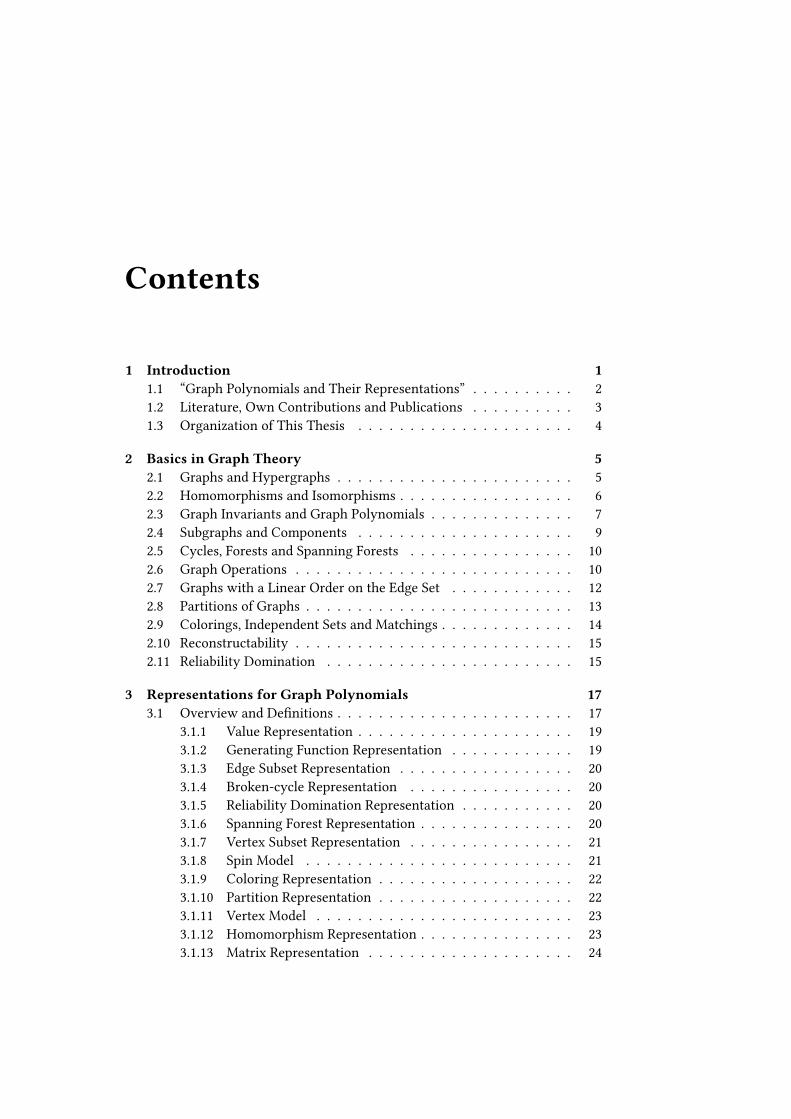
Contents
1 Introduction 11.1 “Graph Polynomials and Their Representations” . . . . . . . . . . 21.2 Literature, Own Contributions and Publications . . . . . . . . . . 31.3 Organization of This Thesis . . . . . . . . . . . . . . . . . . . . . 4
2 Basics in Graph Theory 52.1 Graphs and Hypergraphs . . . . . . . . . . . . . . . . . . . . . . . 52.2 Homomorphisms and Isomorphisms . . . . . . . . . . . . . . . . . 62.3 Graph Invariants and Graph Polynomials . . . . . . . . . . . . . . 72.4 Subgraphs and Components . . . . . . . . . . . . . . . . . . . . . 92.5 Cycles, Forests and Spanning Forests . . . . . . . . . . . . . . . . 102.6 Graph Operations . . . . . . . . . . . . . . . . . . . . . . . . . . . 102.7 Graphs with a Linear Order on the Edge Set . . . . . . . . . . . . 122.8 Partitions of Graphs . . . . . . . . . . . . . . . . . . . . . . . . . . 132.9 Colorings, Independent Sets and Matchings . . . . . . . . . . . . . 142.10 Reconstructability . . . . . . . . . . . . . . . . . . . . . . . . . . . 152.11 Reliability Domination . . . . . . . . . . . . . . . . . . . . . . . . 15
3 Representations for Graph Polynomials 173.1 Overview and DeVnitions . . . . . . . . . . . . . . . . . . . . . . . 17
3.1.1 Value Representation . . . . . . . . . . . . . . . . . . . . . 193.1.2 Generating Function Representation . . . . . . . . . . . . 193.1.3 Edge Subset Representation . . . . . . . . . . . . . . . . . 203.1.4 Broken-cycle Representation . . . . . . . . . . . . . . . . 203.1.5 Reliability Domination Representation . . . . . . . . . . . 203.1.6 Spanning Forest Representation . . . . . . . . . . . . . . . 203.1.7 Vertex Subset Representation . . . . . . . . . . . . . . . . 213.1.8 Spin Model . . . . . . . . . . . . . . . . . . . . . . . . . . 213.1.9 Coloring Representation . . . . . . . . . . . . . . . . . . . 223.1.10 Partition Representation . . . . . . . . . . . . . . . . . . . 223.1.11 Vertex Model . . . . . . . . . . . . . . . . . . . . . . . . . 233.1.12 Homomorphism Representation . . . . . . . . . . . . . . . 233.1.13 Matrix Representation . . . . . . . . . . . . . . . . . . . . 24

viii CONTENTS
3.1.14 Matroid Representation . . . . . . . . . . . . . . . . . . . 253.1.15 Recurrence Relation Representation . . . . . . . . . . . . 25
3.2 Relations to the Edge Subset Representation . . . . . . . . . . . . 253.2.1 Broken-cycle Representation . . . . . . . . . . . . . . . . 263.2.2 Spanning Forest Representation . . . . . . . . . . . . . . . 303.2.3 Reliability Domination Representation . . . . . . . . . . . 35
3.3 Recurrence Relations . . . . . . . . . . . . . . . . . . . . . . . . . 373.3.1 Some Examples . . . . . . . . . . . . . . . . . . . . . . . . 383.3.2 Two General Theorems . . . . . . . . . . . . . . . . . . . 39
4 Edge Elimination Polynomials 434.1 The Edge Elimination Polynomial . . . . . . . . . . . . . . . . . . 444.2 The Covered Components Polynomial . . . . . . . . . . . . . . . . 454.3 The Subgraph Counting Polynomial . . . . . . . . . . . . . . . . . 474.4 The Extended Subgraph Counting Polynomial . . . . . . . . . . . 494.5 The Trivariate Chromatic Polynomial . . . . . . . . . . . . . . . . 514.6 Further Edge Elimination Polynomials . . . . . . . . . . . . . . . . 55
4.6.1 The Hyperedge Elimination Polynomial . . . . . . . . . . 554.6.2 The Subgraph Enumerating Polynomial . . . . . . . . . . 564.6.3 The Trivariate Chromatic Polynomial by White . . . . . . 57
4.7 Properties . . . . . . . . . . . . . . . . . . . . . . . . . . . . . . . 574.7.1 Encoded Invariants . . . . . . . . . . . . . . . . . . . . . . 574.7.2 Derivatives . . . . . . . . . . . . . . . . . . . . . . . . . . 594.7.3 Reconstructability . . . . . . . . . . . . . . . . . . . . . . 60
4.8 Relations . . . . . . . . . . . . . . . . . . . . . . . . . . . . . . . . 624.8.1 Relation to the U-polynomial . . . . . . . . . . . . . . . . 624.8.2 Relation to the Chromatic Symmetric Function . . . . . . 634.8.3 Relation to the Subgraph Component Polynomial . . . . . 644.8.4 Relation to the Extended Negami Polynomial . . . . . . . 664.8.5 Relation to the Bivariate Chromatic Polynomial . . . . . . 674.8.6 Relation to the Wiener Polynomial . . . . . . . . . . . . . 68
5 The Generalized Subgraph Counting Polynomial 715.1 DeVnition and Recurrence Relation . . . . . . . . . . . . . . . . . 715.2 Relations . . . . . . . . . . . . . . . . . . . . . . . . . . . . . . . . 735.3 Properties . . . . . . . . . . . . . . . . . . . . . . . . . . . . . . . 77
5.3.1 Polynomial Reconstructability . . . . . . . . . . . . . . . . 775.3.2 Non-isomorphic Graphs with Coinciding Generalized
Subgraph Counting Polynomial . . . . . . . . . . . . . . . 775.3.3 Not Necessarily a “Most General” Graph Polynomial . . . 78
6 Conclusion 836.1 An Overview about Graph Polynomials . . . . . . . . . . . . . . . 846.2 Open Problems . . . . . . . . . . . . . . . . . . . . . . . . . . . . . 84

CONTENTS ix
A List of Graph Polynomials 87
Glossary 95
Bibliography 99

x CONTENTS
Chapter 1
Introduction
In graph theory, as in discrete mathematics in general, not only the existence, butalso the counting of objects with some given properties, is of main interest. Tocount and to encode the number of structures with given properties, generatingfunctions, formally written as polynomials, are widely used. With respect tographs, we speak about graph polynomials that count the number of subgraphswith given properties.
A graph can nowadays be easily described as the abstraction of a network. Itconsists of a set of vertices and a set of edges, where each edge connects at mosttwo vertices with each other. A graph polynomial is a polynomial associatedto a graph, such that the same polynomial is assigned to graphs arising from arelabeling of the vertices.
While some graph polynomials, for instance the characteristic polynomial,the chromatic polynomial, the matching polynomial and the Tutte polynomial,are already studied intensively and also their relations are well known, this doesnot hold for graph polynomials in general. In fact, as more and more speciVcgraph structures, and consequently the corresponding subgraphs, have been an-alyzed, for many of these a generating function and thereby a graph polynomialhas been deVned. Hence, there is a multitude of graph polynomials — called “thezoo of graph polynomials” following a suggestion of Zaslavsky [99, footnote onpage 1] — whose similarities and diUerences, and hence whose relations, are notyet clariVed.
The main aim of this dissertation is to give a substantial contribution to thelong-term goal of establishing a “general theory of graph polynomials”, a termused by Makowsky in the title of [100]. It is clear, that this will not be possiblein an one-to-one-meaning, as the nature of graph polynomials diUers extremelydepending on the context in which these are deVned.
We have both perspectives on graph polynomials, a very general one by ob-serving in which frameworks graph polynomials can be deVned, and a very spe-ciVc one exploring a speciVc graph polynomial, the edge elimination polynomial.We bring both perspectives together by introducing several graph polynomials

2 CHAPTER 1. INTRODUCTION
which are equivalent to the edge elimination polynomial, that means these canbe calculated (for a given graph) from the edge elimination polynomial (of thisgraph) and vice versa, but are deVned in diUerent frameworks. By using anappropriate graph polynomial we can show some properties valid for all theseequivalent graph polynomials, which may be much harder to prove starting fromanother deVnition. These results provide some evidence that it makes sense toconsider equivalent graph polynomials.
Related to this is the topic of recurrence relations for graph polynomials.These either can be stated for given graph polynomials, or can be used to deVnesome. While in the Vrst case, the problem to Vnd (and prove) a recurrence re-lation, in the second case, to Vnd a combinatorial interpretation of the speciVedgraph polynomial may be challenging. Again, we give some general results onrecurrence relations and some speciVc results on single graph polynomials.
Another focus lies on the deVnition of (slightly more general) graph polyno-mials unifying several of the major graph polynomials. Regarding this, we deVnethe generalized subgraph counting polynomial. This graph polynomial gener-alizes two classes of graph polynomials, those satisfying a recurrence relationwith respect to some edge operations and those satisfying a recurrence relationwith respect to some vertex operations. We prove that the generalized subgraphcounting polynomial itself also obeys a recurrence relation.
While we have mentioned only graphs until now, many results are also validfor the more general case of hypergraphs, where in a hypergraph each edge maybe connect an arbitrary number of vertices.
1.1 “Graph Polynomials and Their Representations”
The title of this dissertation is chosen to include two possible meanings of theterm “representation” in connection with graph polynomials.
Mainly, by “representations for graph polynomials” we mean the frameworks(ways, formalisms, concepts) used to deVne graph polynomials. Thus, we aretalking about an “edge subset representation” and a “coloring representation” if agraph polynomial is deVned as a sum over edge subsets and as a sum over color-ings, respectively. As the name suggests, the chromatic polynomial is originallydeVned in terms of colorings and therefore by a coloring representation.
Furthermore, it seems to be possible to expand this meaning and to refer to agraph polynomial equivalent to another graph polynomial, but deVned in anotherframework (representation), as a “representation” of the given graph polynomial.With this meaning, a representation of the chromatic polynomial is for examplethe adjoint polynomial, which is deVned as a sum over partitions and can bederived from the chromatic polynomial by replacing the falling factorials in anappropriate formulation by powers, and vice versa.
Another frequently used term is an “expansion” of a graph polynomial, whichdenotes an equivalent graph polynomial (deVned in another framework) yielding
1.2. LITERATURE, OWN CONTRIBUTIONS AND PUBLICATIONS 3
exactly the same graph polynomial. Many expansions of the chromatic poly-nomial are known, including an “edge subset expansion” stating the chromaticpolynomial as a sum over edge subsets.
While the term “representation” is rarely used in the literature and not nec-essarily in the same meaning, the term “expansion” with respect to graph poly-nomials is widely used with the same meaning. As an example, in the article “Ex-pansions of the chromatic polynomial” Biggs [14] states several diUerent waysthe chromatic polynomial can be deVned. The Vrst usage in this direction seemsto be Whitney’s “A logical expansion in mathematics” [152], where the edge sub-set expansion and the broken-cycle expansion of the chromatic polynomial aregiven (not using these terms explicitly). The term is often used as “subset expan-sion”, which half the times denotes what we denote as “edge subset expansion”,but in the other cases refers to a sum or product over some other ground set thanthe edge set.
A related term is “type analog”, which is used by Sarmiento [122] to expressthat (two) graph polynomials are stated using similar formalisms: “That is, bothpolynomials ‘look similar’ in the sense that” replacing some term by another, onegraph polynomial is transformed into another.
1.2 Literature, Own Contributions and Publications
The point of origin of the present research was the deVnition of the edge elimina-tion polynomial in connection with the search for graph polynomials satisfyingsome recurrence relations and relations between graph polynomials followingfrom such recurrence relations. Namely we want to mention the following liter-ature:
• “From a zoo to a zoology: Towards a general theory of graph polynomials”[100],
• “A most general edge elimination polynomial” and “An extension of the bi-variate chromatic polynomial”, both introducing the edge elimination poly-nomial [4; 5],
• some surveys on graph polynomials [54; 55; 108; 113].
My own contributions are in particular the deVnition of the covered com-ponents polynomial, the subgraph counting polynomial, the trivariate chromaticpolynomial (all equivalent to the edge elimination polynomial) and the gener-alized subgraph counting polynomial, together with the statement concerningthese graph polynomials.
Some of these results are already published or submitted:
• “The covered components polynomial: A new representation of the edgeelimination polynomial”, introducing the covered components polynomial,published as [139],
4 CHAPTER 1. INTRODUCTION
• “From spanning forests to edge subsets”, relating spanning forest repre-sentation and edge subset representation, a preprint is published as [137],submitted to Ars Mathematica Contemporanea,
• “Proving properties of the edge elimination polynomial using equivalentgraph polynomials”, introducing the subgraph counting polynomial andthe trivariate chromatic polynomial, a preprint is published as [138], sub-mitted to Congressus Numerantium.
1.3 Organization of This Thesis
This thesis consists of six chapters and one appendix, where Chapter 2 and Chap-ter 6 provide the necessary terms and a conclusion, respectively. The chaptersbetween are mostly self-contained and can be read in arbitrary order, while thegiven order is the one suggested.
In Chapter 2, all deVnitions and notations used throughout the work, withexception of the deVnition of the graph polynomials, are given.
Then we investigate possible ways to deVne graph polynomials, the represen-tations for graph polynomials, in Chapter 3. The Vrst section is in an extensive butnot exhaustive overview about the frameworks used in the literature, expandedby some Vrst classiVcation of them. Relations between representations are givenin the second section. The third section is especially devoted to recurrence rela-tions.
In Chapter 4, the edge elimination polynomials are considered, which in-clude the edge elimination polynomial and the graph polynomials equivalent toit. We start with a short introduction of the edge elimination polynomial andthen present several equivalent graph polynomials. Their combinatorial inter-pretations are used to prove some properties valid for all edge elimination poly-nomials and some relations to other graph polynomials.
A new graph polynomial, the generalized subgraph counting polynomial, isdeVned in Chapter 5. This proceeds the results of the previous chapter as itgeneralizes some of them. The main theorem there is the recurrence relationapplicable also for hypergraphs, which easily enables to derive many well-knowngraph polynomials and their recurrence relations from it.
For the sake of convenience, in Appendix A we itemize references and deVni-tions for all mentioned graph polynomials, and in the Glossary the occurrences ofthe signiVcant terms, including the representations, expansions and graph poly-nomials, are given.
Chapter 2
Basics in Graph Theory
In this chapter we introduce some graph theory we make use of. Because we dis-cuss a multitude of diUerent graphs polynomials, we touch a lot of miscellaneousareas of graph theory, and, consequently, a long list of deVnitions and notationsis necessary.
While we try to deVne every term applied, previous knowledge of graph the-ory as presented in standard textbooks [10; 15; 25; 28; 47; 65; 144] may be advan-tageous. Readers familiar with this topic may skip to the next chapter.
For the sake of convenience, we use the terms used for graphs also for hyper-graphs, for example we speak about “graph polynomial” and “subgraph” instead“hypergraph polynomials” and “subhypergraphs”. Consequently, correspondingtheorems will only diUer on the assumption of a graph or a hypergraph.
Preliminary, we present the following (non-graph-theoretic) notations: Forelements s1 , . . . , sk , by {s1 , . . . , sk } and {s1 , . . . , sk }∗ we denote the set and themultiset of these elements, and by |{s1 , . . . , sk }| and |{s1 , . . . , sk }∗ | we denote theircardinality, respectively. For sets A, B (with A ⊆ B), the interval [A, B] is the setof subsets of B, which are supersets of A. For a set S ,
(Sk
)denotes the set of k-
element subsets of S . For a statement S , let [S] be equal to 1, if S is true, and 0otherwise [86].
2.1 Graphs and Hypergraphs
DeVnition 2.1. A graph G = (V , E) is an ordered pair of a set of vertices, thevertex setV , and a multiset of edges, the edge set E, such that each edge is a one-or two-element subset of the vertex set, i.e. e ∈
(V1
)∪
(V2
)for all e ∈ E. An edge
e ∈ E is a link, if it is a two-element subsets of V , i.e. e ∈(V2
), and a loop, if it is
an one-element subset of V , i.e. e ∈(V1
).
DeVnition 2.2. A simple graph is a graph G = (V , E), where each edge is a linkand the edge set is a set, i.e. E ⊆
(V2
).
6 CHAPTER 2. BASICS IN GRAPH THEORY
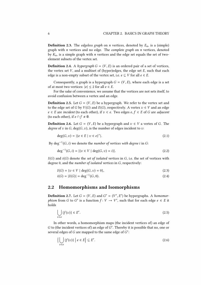
DeVnition 2.3. The edgeless graph on n vertices, denoted by En , is a (simple)graph with n vertices and no edge. The complete graph on n vertices, denotedby Kn , is a simple graph with n vertices and the edge set equals the set of two-element subsets of the vertex set.
DeVnition 2.4. A hypergraph G = (V , E) is an ordered pair of a set of vertices,the vertex set V , and a multiset of (hyper)edges, the edge set E, such that eachedge is a non-empty subset of the vertex set, i.e. e ⊆ V for all e ∈ E.
Consequently, a graph is a hypergraph G = (V , E), where each edge is a setof at most two vertices: |e | ≤ 2 for all e ∈ E.
For the sake of convenience, we assume that the vertices are not sets itself, toavoid confusion between a vertex and an edge.
DeVnition 2.5. Let G = (V , E) be a hypergraph. We refer to the vertex set andto the edge set of G by V (G ) and E (G ), respectively. A vertex v ∈ V and an edgee ∈ E are incident (to each other), if v ∈ e . Two edges e , f ∈ E of G are adjacent(to each other), if e ∩ f , ∅.
DeVnition 2.6. Let G = (V , E) be a hypergraph and v ∈ V a vertex of G. Thedegree of v in G, deg(G ,v ), is the number of edges incident to v :
deg(G ,v ) = |{e ∈ E | v ∈ e}∗ |. (2.1)
By deg−1 (G , i ) we denote the number of vertices with degree i in G:
deg−1 (G , i ) = |{v ∈ V | deg(G ,v ) = i}|. (2.2)
I (G ) and i (G ) denote the set of isolated vertices in G, i.e. the set of vertices withdegree 0, and the number of isolated vertices in G, respectively:
I (G ) = {v ∈ V | deg(G ,v ) = 0}, (2.3)
i (G ) = |I (G ) | = deg−1 (G , 0). (2.4)
2.2 Homomorphisms and Isomorphisms
DeVnition 2.7. Let G = (V , E) and G′ = (V ′, E′) be hypergraphs. A homomor-phism from G to G′ is a function f : V → V ′, such that for each edge e ∈ E itholds ⋃
v∈e
{f (v )} ∈ E′. (2.5)
In other words, a homomorphism maps (the incident vertices of) an edge ofG to (the incident vertices of) an edge ofG′. Thereby it is possible that no, one orseveral edges of G are mapped to the same edge of G′:{⋃
v∈e
{f (v )}∣∣∣ e ∈ E} ⊆ E′. (2.6)

2.3. GRAPH INVARIANTS AND GRAPH POLYNOMIALS 7
For the counting of homomorphisms it is usual to also consider which edge ofG is mapped to which edge ofG′, that means to count functions mapping verticesto vertices and edges to edges.
DeVnition 2.8. Let G = (V , E) and G′ = (V ′, E′) be hypergraphs. The numberof homomorphisms from G to G′, denoted by hom(G ,G′), is deVned as
hom(G ,G′) =∑
f :{V →V ′E→E′
[∀v ∈ V ∀e ∈ E : v ∈ e ⇒ f (v ) ∈ f (e )]. (2.7)
For simple graphs G and G′ (in fact if G′ has no parallel edges), a homomor-phism is given by the function mapping the vertex sets. Hence,
hom(G ,G′) =∑
f : V →V ′
[∀e ∈ E :
⋃v∈e
{f (v )} ∈ E′]. (2.8)
This can be extended to the general case of hypergraphs by considering thenumber of edges of E′, to which each edge of E can be mapped:
hom(G ,G′) =∑
f : V →V ′
∏e∈E
∣∣∣∣{e′ ∈ E′ : ⋃v∈e
{f (v )
}= e′
}∗∣∣∣∣. (2.9)
This deVnition is similar to those used by Garijo, Goodall and Nešetřil [59,Subsection 2.1].
DeVnition 2.9. Let G = (V , E) and G′ = (V ′, E′) be hypergraphs. An isomor-phism from G into G′ is a bijective homomorphism, that is a bijective functionf : V → V ′, such that{⋃
v∈e
{f (v )}∣∣∣ e ∈ E}∗ = E′. (2.10)
The hypergraphsG andG′ are isomorphic, if there is an isomorphism fromG intoG′.
In other words,G andG′ are isomorphic, ifG′ can be obtained by a relabelingof the vertices of G.
2.3 Graph Invariants and Graph Polynomials
DeVnition 2.10. Let G be the set of hypergraphs and S some set. A graphinvariant is a function f : G → S, such that for isomorphic graphs G ,G′ ∈ G itholds
f (G ) = f (G′). (2.11)

8 CHAPTER 2. BASICS IN GRAPH THEORY
DeVnition 2.11. Let G be the set of hypergraphs and R[x1 , . . . , xk ] the ringof polynomials in the commuting variables x1 , . . . , xk over the real numbers. Agraph polynomial P (G , x1 , . . . , xk ) is a function P : G → R[x1 , . . . , xk ].
DeVnition 2.12. Let G be the set of hypergraphs. An invariant graph polynomialis a graph polynomial, which is a graph invariant, that is a function P : G →R[x1 , . . . , xk ], such that for isomorphic hypergraphs G ,G′ ∈ G and commutingvariables x1 , . . . , xk it holds
P (G , x1 , . . . , xk ) = P (G′, x1 , . . . , xk ). (2.12)
Until otherwise stated, we consider only graph polynomials, which are alsograph invariants, and therefore use “graph polynomial” as abbreviation for “in-variant graph polynomial”. In case of S = {0, 1} and S = N one usually speaksabout (invariant) graph properties and (invariant) graph parameters, respectively.While we consider polynomial rings over the real numbers for the deVnition,the coeXcients of the graph polynomials investigated in the following are in-tegers. Furthermore, all variables are commuting, and in case of multivariatepolynomials we deVne X = (x1 , . . . , xk ) and write R[X ] and P (G ,X ) instead ofR[x1 , . . . , xk ] and P (G , x1 , . . . , xk ), respectively. In particular, by P (G ,X ) we de-note an arbitrary graph polynomial. Additionally, we use P (G ,X ,y) for a graphpolynomial in the variables x1 , . . . , xk ,y.
DeVnition 2.13. Let G be the set of hypergraphs and P (G ,X ), P ′(G ,X ) twograph polynomials. P (G ,X ) and P ′(G ,X ) are equivalent (to each other), if thereis a bijection f : R[X ]→ R[X ], such that for all graphs G ∈ G it holds
P (G ,X ) = f (P ′(G ,X )). (2.13)
DeVnition 2.14. Let P = P (G ,X ) be a (graph) polynomial with
P =∑
i1 ,...,ik
ai1 ,...,ikxi11 · · · x
ikk , (2.14)
where i1 , . . . , ik ∈ N and ai1 ,...,ik ∈ R. We denote by degx (P ) the degree of x inP and by [xlj ](P ) the sum of all monomials including the variable xj in the powerl , i.e.
[xlj ](P ) =∑
i1 ,...,ikij=l
ai1 ,...,ikxi11 · · · x
ij−1j−1 x
ij+1j+1 · · · x
ikk . (2.15)
Furthermore, we expand this to several variables and write [xi11 · · · xijj ](P ) instead
of [xi11 ](· · · [xijj ](P ) · · · ).
For a graph polynomial P (G , x ) in a single variable x , [xi ](P (G , x )) is thecoeXcient of xi in P (G , x ).
2.4. SUBGRAPHS AND COMPONENTS 9
2.4 Subgraphs and Components
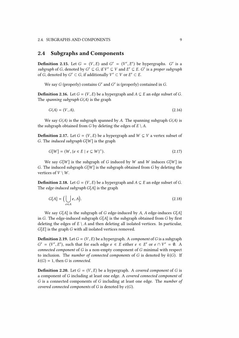
DeVnition 2.15. Let G = (V , E) and G′ = (V ′, E′) be hypergraphs. G′ is asubgraph of G, denoted by G′ ⊆ G, if V ′ ⊆ V and E′ ⊆ E. G′ is a proper subgraphof G, denoted by G′ ⊂ G, if additionally V ′ ⊂ V or E′ ⊂ E.
We say G (properly) contains G′ and G′ is (properly) contained in G.
DeVnition 2.16. LetG = (V , E) be a hypergraph and A ⊆ E an edge subset ofG.The spanning subgraph G〈A〉 is the graph
G〈A〉 = (V ,A). (2.16)
We say G〈A〉 is the subgraph spanned by A. The spanning subgraph G〈A〉 isthe subgraph obtained from G by deleting the edges of E \A.
DeVnition 2.17. Let G = (V , E) be a hypergraph andW ⊆ V a vertex subset ofG. The induced subgraph G[W ] is the graph
G[W ] = (W , {e ∈ E | e ⊆W }∗ ). (2.17)
We say G[W ] is the subgraph of G induced by W and W induces G[W ] inG. The induced subgraph G[W ] is the subgraph obtained from G by deleting thevertices of V \W .
DeVnition 2.18. LetG = (V , E) be a hypergraph and A ⊆ E an edge subset ofG.The edge-induced subgraph G[A] is the graph
G[A] =( ⋃e∈A
e ,A). (2.18)
We say G[A] is the subgraph of G edge-induced by A, A edge-induces G[A]in G. The edge-induced subgraph G[A] is the subgraph obtained from G by Vrstdeleting the edges of E \ A and then deleting all isolated vertices. In particular,G[E] is the graph G with all isolated vertices removed.
DeVnition 2.19. LetG = (V , E) be a hypergraph. A component ofG is a subgraphG′ = (V ′, E′), such that for each edge e ∈ E either e ∈ E′ or e ∩ V ′ = ∅. Aconnected component of G is a non-empty component of G minimal with respectto inclusion. The number of connected components of G is denoted by k (G ). Ifk (G ) = 1, then G is connected.
DeVnition 2.20. Let G = (V , E) be a hypergraph. A covered component of G isa component of G including at least one edge. A covered connected component ofG is a connected components of G including at least one edge. The number ofcovered connected components of G is denoted by c (G ).

10 CHAPTER 2. BASICS IN GRAPH THEORY
Remarks
Please note that especially for the diUerent kind of subgraphs the notation is notuniform in diUerent textbooks, see [11, Section 1.1; 25, Section I.1; 28, Section 2.1,2.2; 47, Section 1.1; 65, Section 1.2; 144, Section I.3].
2.5 Cycles, Forests and Spanning Forests
DeVnition 2.21. Let G = (V , E) be a graph. G is cyclic, if G has a subgraphG′ = (V ′, E′) including at least one edge, such that for each edge e ∈ E′ of G′ itholds
k (G′) = k (G′−e ). (2.19)
Otherwise, G is acyclic.
DeVnition 2.22. Let G = (V , E) be a graph. G is a cycle, if G is cyclic and has noproper cyclic subgraph. G is a forest, if G is acyclic. G is tree, if G is acyclic andconnected.
DeVnition 2.23. Let G = (V , E) be a graph and A ⊆ E an edge subset of G. AtreeT = G〈A〉 = (V ,A) is a spanning tree ofG. The set of all spanning trees ofG isdenoted by T (G ).
DeVnition 2.24. Let G = (V , E) be a graph and A ⊆ E an edge subset of G. Aforest F = G〈A〉 = (V ,A) is a spanning forest of G, if k (G ) = k (F ). The set of allspanning forests of G is denoted by F (G ).
Remarks
While the term “spanning tree” is unambiguous, the term “spanning forest” is not,because not every spanning subgraph which is a forest is a “spanning forest” [25,Section X.5]. A spanning forest is the union of spanning trees for each connectedcomponent.
2.6 Graph Operations
DeVnition 2.25. Let G = (V , E) and G′ = (V ′, E′) be hypergraphs. The unionG ∪G′ is the graph arising from the union of the vertex sets and edge sets:
G ∪G′ = (V ∪V ′, E ∪ E′). (2.20)
DeVnition 2.26. Let G = (V , E) and G′ = (V ′, E′) be hypergraphs. The intersec-tion G ∩G′ is the graph arising from the intersection of the vertex sets and edgesets:
G ∩G′ = (V ∩V ′, E ∩ E′). (2.21)

2.6. GRAPH OPERATIONS 11
DeVnition 2.27. Let G = (V , E) and G′ = (V ′, E′) be hypergraphs. The disjointunion G∪· G′ is the graph arising from the union of disjoint copies of both graphs.
In other words, Vrst (the vertices of) the graphs are relabeled, such that theintersection of both graphs is empty, and then the union is formed.
DeVnition 2.28. Let G = (V , E) be a hypergraph and e ∈ E an edge of G. WedeVne the following edge operations:
• −e: deletion of the edge e , i.e. e is removed,
• /e: contraction of the edge e , i.e. e is removed and its incident vertices aremerged (parallel edges and loops may occur),
• †e: extraction of the edge e , i.e. the vertices incident to e and their incidentedges (including e itself) are removed.
The arising hypergraphs are denoted by G−e , G/e and G†e , respectively.
DeVnition 2.29. Let G = (V , E) be a hypergraph and e ⊆ V a possible edge of G(with respect to the type of graph). We deVne the following non-edge operations:
• +e: insertion of the edge e , i.e. e is added,
• /e: contraction of the vertices in e , i.e. the vertices in e are merged (paralleledges and loops may occur),
The arising hypergraphs are denoted by G+e and G/e , respectively.
DeVnition 2.30. Let G = (V , E) be a hypergraph, v ∈ V a vertex and W ⊆ V avertex subset of G. We deVne the following vertex operations:
• v : deletion of the vertex v , i.e. v and its incident edges are removed,
• W : deletion of all vertices in the vertex subset W , i.e. all vertices v ∈ Wand their incident edges are removed.
The arising hypergraphs are denoted by Gv and GW , respectively.
Remarks
We use W instead of the usual −W for the deletion of the vertex setW from agraph G = (V , E), because each edge is also a vertex subset, and therefore withW = e ∈ E we have to distinguish between the deletion of the edge e , −e , and thedeletion of the vertices incident to the edge e , e . For probably similar reasonsthis notation is already used in the literature [57; 80]. It holds G†e = Ge , butthe Vrst term is deVned only for e ∈ E, whereas the second one is deVned for anye ⊆ V .

12 CHAPTER 2. BASICS IN GRAPH THEORY
The deVned edge and vertex operations are known from the recurrence rela-tions for the chromatic polynomial, see Section 3.3, the matching polynomial [56,Theorem 1] and the independence polynomial [68, Proposition 4].
There are several more graph operations that can be found in the literature,for example:
• vertex contraction [134, Section 5.1],
• insertion of “pseudo-edges” [9, Section 1],
• Kellman’s operation (for adjacent vertices) [43, DeVnition 2.0.1]
• NA-Kellman’s operation (for non-adjacent vertices) [43, DeVnition 2.8.1],
• adaption of two vertices [34, Section 3],
• cloning of edges and vertices [78, Section 3].
2.7 Graphs with a Linear Order on the Edge Set
In the following we consider graphsG = (V , E) with a linear order < on the edgeset E. This linear order can be represented by a bijection β : E → {1, . . . , |E |} forall e , f ∈ E with
e < f ⇔ β (e ) < β (f ). (2.22)
DeVnition 2.31 (Section 7 in [152]). Let G = (V , E) be a graph with a linearorder < on the edge set E. Let C = (VC , EC ) ⊆ G be a cycle and e ∈ EC themaximal edge of C with respect to <. Then EC \ {e} is a broken cycle in G withrespect to <. The set of all broken cycles of G with respect to < is denoted byB (G , <).
DeVnition 2.32 (Section 3 in [141]). Let G = (V , E) be a graph with a linearorder < on the edge set E and F = (V ,A) ∈ F (G ) a spanning forest of G. Anedge e ∈ A is internally active in F with respect toG and <, if there exists no edgef ∈ E \ A, such that e < f and F−e+f ∈ F (G ). We denote the set of internallyactive edges and the number of internally active edges of F with respect to G and< by Ei (F ,G , <) and i (F ,G , <), respectively.
An edge e in the spanning forest F is internally active, if it is the maximaledge of all edges in the cut crossed by e itself (connecting the vertices in theconnected components arising by deleting e from F ). In other words, the edgee can not be replaced by a greater edge (not in the spanning forest), such that Fremains a spanning forest. Hence, formally we have
Ei (F ,G , <) = {e ∈ E (F ) | @f ∈ E (G ) \ E (F ) : e < f ∧ F−e+f ∈ F (G )}.(2.23)
2.8. PARTITIONS OF GRAPHS 13
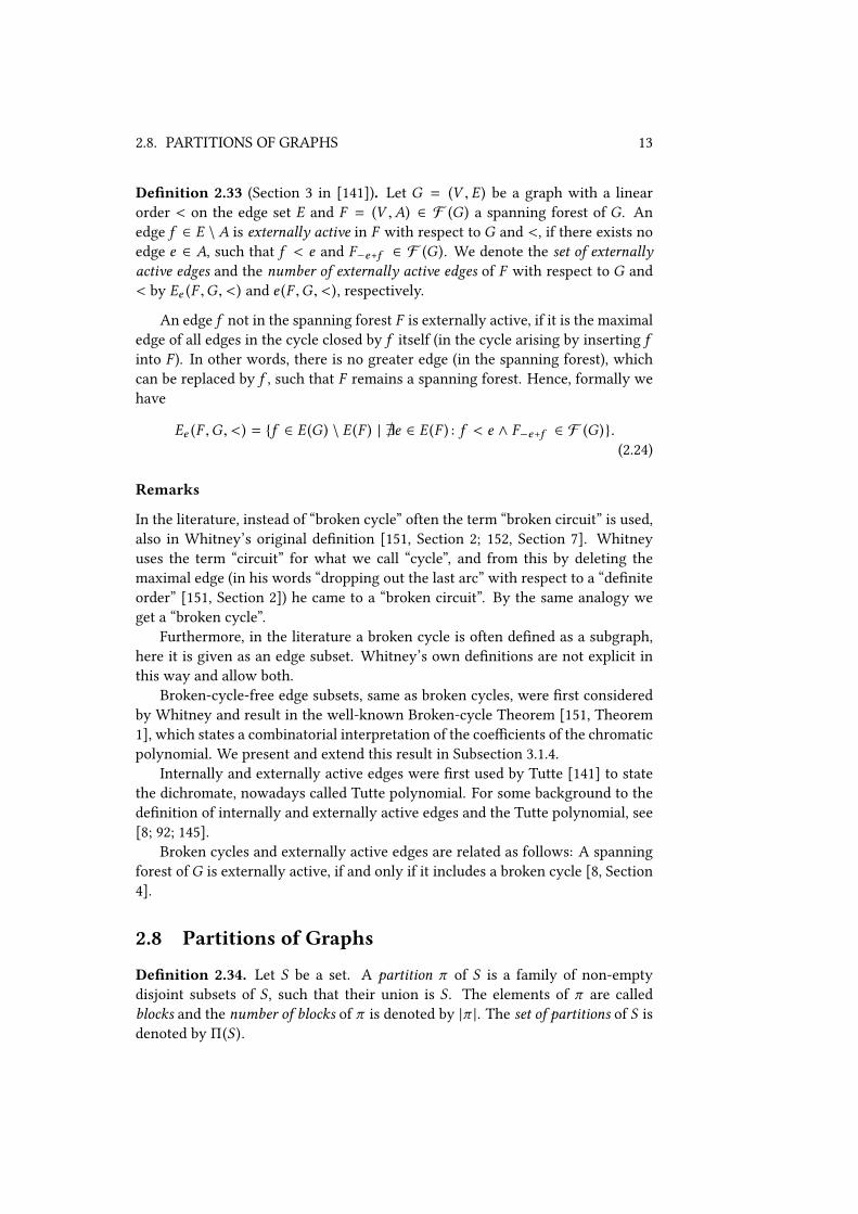
DeVnition 2.33 (Section 3 in [141]). Let G = (V , E) be a graph with a linearorder < on the edge set E and F = (V ,A) ∈ F (G ) a spanning forest of G. Anedge f ∈ E \A is externally active in F with respect to G and <, if there exists noedge e ∈ A, such that f < e and F−e+f ∈ F (G ). We denote the set of externallyactive edges and the number of externally active edges of F with respect to G and< by Ee (F ,G , <) and e (F ,G , <), respectively.
An edge f not in the spanning forest F is externally active, if it is the maximaledge of all edges in the cycle closed by f itself (in the cycle arising by inserting finto F ). In other words, there is no greater edge (in the spanning forest), whichcan be replaced by f , such that F remains a spanning forest. Hence, formally wehave
Ee (F ,G , <) = {f ∈ E (G ) \ E (F ) | @e ∈ E (F ) : f < e ∧ F−e+f ∈ F (G )}.(2.24)
Remarks
In the literature, instead of “broken cycle” often the term “broken circuit” is used,also in Whitney’s original deVnition [151, Section 2; 152, Section 7]. Whitneyuses the term “circuit” for what we call “cycle”, and from this by deleting themaximal edge (in his words “dropping out the last arc” with respect to a “deVniteorder” [151, Section 2]) he came to a “broken circuit”. By the same analogy weget a “broken cycle”.
Furthermore, in the literature a broken cycle is often deVned as a subgraph,here it is given as an edge subset. Whitney’s own deVnitions are not explicit inthis way and allow both.
Broken-cycle-free edge subsets, same as broken cycles, were Vrst consideredby Whitney and result in the well-known Broken-cycle Theorem [151, Theorem1], which states a combinatorial interpretation of the coeXcients of the chromaticpolynomial. We present and extend this result in Subsection 3.1.4.
Internally and externally active edges were Vrst used by Tutte [141] to statethe dichromate, nowadays called Tutte polynomial. For some background to thedeVnition of internally and externally active edges and the Tutte polynomial, see[8; 92; 145].
Broken cycles and externally active edges are related as follows: A spanningforest ofG is externally active, if and only if it includes a broken cycle [8, Section4].
2.8 Partitions of Graphs
DeVnition 2.34. Let S be a set. A partition π of S is a family of non-emptydisjoint subsets of S , such that their union is S . The elements of π are calledblocks and the number of blocks of π is denoted by |π |. The set of partitions of S isdenoted by Π(S ).
14 CHAPTER 2. BASICS IN GRAPH THEORY
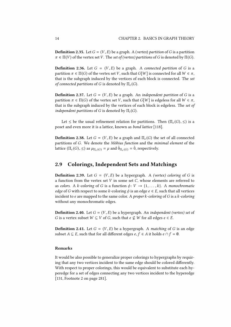
DeVnition 2.35. LetG = (V , E) be a graph. A (vertex) partition ofG is a partitionπ ∈ Π(V ) of the vertex setV . The set of (vertex) partitions ofG is denoted by Π(G ).
DeVnition 2.36. Let G = (V , E) be a graph. A connected partition of G is apartition π ∈ Π(G ) of the vertex setV , such thatG[W ] is connected for allW ∈ π ,that is the subgraph induced by the vertices of each block is connected. The setof connected partitions of G is denoted by Πc (G ).
DeVnition 2.37. Let G = (V , E) be a graph. An independent partition of G is apartition π ∈ Π(G ) of the vertex set V , such that G[W ] is edgeless for allW ∈ π ,that is the subgraph induced by the vertices of each block is edgeless. The set ofindependent partitions of G is denoted by Πi (G ).
Let ≤ be the usual reVnement relation for partitions. Then (Πc (G ), ≤) is aposet and even more it is a lattice, known as bond lattice [118].
DeVnition 2.38. Let G = (V , E) be a graph and Πc (G ) the set of all connectedpartitions of G. We denote the Möbius function and the minimal element of thelattice (Πc (G ) , ≤) as µΠc (G ) = µ and 0Πc (G ) = 0, respectively.
2.9 Colorings, Independent Sets and Matchings
DeVnition 2.39. Let G = (V , E) be a hypergraph. A (vertex) coloring of G isa function from the vertex set V in some set C , whose elements are referred toas colors. A k-coloring of G is a function ϕ : V → {1, . . . , k }. A monochromaticedge ofG with respect to some k-coloring ϕ is an edge e ∈ E, such that all verticesincident to e are mapped to the same color. A proper k-coloring ofG is a k-coloringwithout any monochromatic edges.
DeVnition 2.40. Let G = (V , E) be a hypergraph. An independent (vertex) set ofG is a vertex subsetW ⊆ V of G, such that e *W for all edges e ∈ E.
DeVnition 2.41. Let G = (V , E) be a hypergraph. A matching of G is an edgesubset A ⊆ E, such that for all diUerent edges e , f ∈ A it holds e ∩ f = ∅.
Remarks
It would be also possible to generalize proper colorings to hypergraphs by requir-ing that any two vertices incident to the same edge should be colored diUerently.With respect to proper colorings, this would be equivalent to substitute each hy-peredge for a set of edges connecting any two vertices incident to the hyperedge[131, Footnote 2 on page 281].

2.10. RECONSTRUCTABILITY 15
2.10 Reconstructability
The reconstruction conjecture of Kelly [85] and Ulam [146] states that every graphG = (V , E) with at least three vertices can be reconstructed from (the isomor-phism classes) of its deckD (G ), which is the multiset of (isomorphism classes) ofvertex-deleted subgraphs, i.e. D (G ) = {Gv | v ∈ V }∗.
This question can be “restricted” to a graph polynomial P (G ,X ) as follows:Can the graph polynomial of a given graph be reconstructed from the graphpolynomials of its deck?
DeVnition 2.42. LetG = (V , E) be a graph and P (G ,X ) a graph polynomial. Thepolynomial deck DP (G ) is the multiset
DP (G ) = {P (Gv ,X ) | v ∈ V }∗ . (2.25)
A graph polynomial is reconstructable from the polynomial deck, if P (G ,X ) can bedetermined from DP (G ).
2.11 Reliability Domination
DeVnition 2.43 (Equation (2.3) in [81]). Let G = (V , E) be a graph, A ⊆ E anedge subset of G and k ∈ N. For all edge subsets B ⊆ A, the signed dominationd (G , B, k ) is recursively deVned by
[k (G〈A〉) ≤ k] =∑B⊆A
d (G , B, k ). (2.26)
Theorem 2.44 (Theorem 4.2 in [81]). Let G = (V , E) be a graph, A ⊆ E an edgesubset of G and k ∈ N. The signed domination d (G ,A, k ) satisVes
d (G ,A, k ) =∑B⊆A
(−1) |A|− |B |[k (G〈B〉) ≤ k]. (2.27)
Proof. The statement follows directly by Möbius inversion. �
DeVnition 2.45 (Proposition 2.8 in [82]). Let G = (V , E) be a graph, A ⊆ E anedge subset ofG and k ∈ N. A k-forest ofG〈A〉 is a spanning subgraphG〈B〉, suchthat G〈B〉 is a forest, B ⊆ A and k (G〈B〉) ≤ k . We denote the set of k-forests ofG〈A〉 by F (G ,A, k ). A k-formation D of G〈A〉 is a non-empty set of k-forests ofG〈A〉, such that their union isG〈A〉, i.e. a non-empty subset F ⊆ F (G ,A, k ) is a k-formation ofG〈A〉, if
⋃H ∈F H = G〈A〉. The set of k-formations ofG〈A〉 is denoted
by D (G ,A, k ). The signed domination d′(G ,A, k ) is deVned as the number of k-formations of G〈A〉 of odd cardinality minus the number of k-formations of G〈A〉of even cardinality, i.e.
d′(G ,A, k ) =∑
D∈D (G,A,k )
(−1) |D |−1. (2.28)

Remarks
Reliability domination has been deVned in order to Vnd a combinatorial inter-pretation of the coeXcients of the reliability polynomial R (G ,p) [124, Equation(7)].
We give two diUerent deVnitions for signed domination and show their equiv-alence in Subsection 3.2.3. Due to Satyanarayana and Tindell [125, Section 1], theoriginal deVnition of signed domination is given by Satyanarayana [123] in termsof “formations” of a graph. It is often deVned with respect to a vertex subset, thisis considered in many publications by Satyanarayana and his coauthors, see [24;116] and the references therein. Another deVnition was given by Huseby [81; 82]for “clutters”. Both deVnitions above orient more on the last one in the case ofgraphs with respect to the number of connected components.
Signed domination is also related to spanning trees: The number of spanningtrees having no externally active edge equals the absolute value of the signeddomination d (G , E , 1) [23, Corollary 4.2].

Chapter 3
Representations forGraph Polynomials
This chapter is devoted to the multitude of diUerent ways and frameworks ap-plied to deVne a graph polynomial — to the representations for graph polynomials.
In Section 3.1 we give a survey on diUerent representations used in the liter-ature. The list does not claim to be exhaustive. However, we hope to mentionthe main representatives available in the literature. For each we give an infor-mal deVnition, an exemplary graph polynomial deVned in this framework, and acorresponding formulation of the chromatic polynomial. Thereby we introduceseveral well-known graph polynomials and expansions of the chromatic polyno-mial.
Some results that serve as a link between the edge subset representation andsome other representations are presented in Section 3.2. With exception of thegeneralization of the Broken-cycle Theorem, the statements are, in principle, al-ready known. However, these statements provide good examples for non-obviousrelations between diUerent representations of graph polynomials and either theproofs, for instance for the relation to reliability domination representation, orthe applications, for instance for the relation to spanning forest representation,seem to be new.
In Section 3.3 we discuss recurrence relations, used to deVne graph polyno-mials or satisVed by them, in more detail. We show some examples and provetwo general results.
3.1 Overview and DeVnitions
There are various ways to deVne graph polynomials and in this section we in-troduce the main patterns we found (with names wherever possible also fromthe literature). The given itemization is neither complete nor are the given rep-resentations formally deVned or disjoint. We also mix between how the graph

18 CHAPTER 3. REPRESENTATIONS FOR GRAPH POLYNOMIALS
polynomials are written down and in which graph theoretic terms these are de-Vned.
For “how the graph polynomials are written down” there are in fact two pos-sibilities: value representation, where the number of the counted objects equalsthe polynomial at a given value, and generating function representation, wherethe number of counted objects equals a coeXcient of a monomial in the polyno-mial. There are also graph polynomials which combine both, for example the badcoloring polynomial which counts for a given number of colors (the variable x )the number of some edges as a generating function (in the variable z).
For the graph theoretic terms used, there are some more possibilities, whichcan be grouped as counting subgraphs, counting mappings and others.
For counting subgraphs, most often spanning subgraphs, given by edge sub-sets, or induced subgraphs, given by a vertex subsets, are considered. Broken-cycles, reliability domination and spanning forests are in fact deVned in terms ofedge subsets, but we list them as single items because of their relevance.
When mappings are counted, there are again three possibilities: mappingsof the vertex set, mappings of the edge set, and homomorphisms to some graph,which are in fact mappings of the vertex and edge set. Spin models (mostlyused for graph polynomials deVned in physics) and colorings are in fact the samekind of vertex mappings, in the Vrst case the vertices are mapped to a set of“spins”, in the second to a set of “colors”. Consequently, both diUer only in their“language”, not in the mathematics behind. We add a superior category denoted“edge mapping representations” to make clear what is meant by a “vertex model”.
The three “other” representations are using matrices and matroids associatedto the graph or recurrence relations.
All together, we classify the representations for graph polynomials as follows:
• value representation,
• generating function representation,
• subgraph representation:
– edge subset representation,
– broken-cycle representation,
– reliability domination representation,
– spanning forest representation,
– vertex subset representation,
• vertex mapping representation:
– spin model,
– coloring representation,
– partition representation,
3.1. OVERVIEW AND DEFINITIONS 19
• edge mapping representation:
– vertex model,
• homomorphism representation.
• matrix representation,
• matroid representation,
• recurrence relation representation,
We continue by introducing the representations, a characteristic graph poly-nomial using this representation, and a corresponding expansion of the chromaticpolynomial one by one. The thereby given list of such expansions is not complete,missing are, amongst others, some subgraph expansions concerning only specialsubgraphs [14; 103].
In the following, we assume G = (V , E) to be a graph with some linear order< on the edge set E. (While most of the deVnitions of graph polynomials alsomake sense in the case of hypergraphs, some expansion would not be valid.)
3.1.1 Value Representation
A value representation states a graph polynomial by a combinatorial interpreta-tion for given values (mostly integers) of the variables.
The chromatic polynomial χ (G , x ) (for x ∈ N) is deVned [18; 52] as the num-ber of proper (vertex) colorings of G with (at most) x colors,
χ (G , x ) = |{proper colorings of G with x colors}|. (3.1)
In fact, from this deVnition it is not obvious that χ (G , x ) is a polynomial in x .
3.1.2 Generating Function Representation
A generating function representation states a graph polynomial as the generatingfunction for a number sequence.
The matching polynomial M (G , x ,y) is deVned [56; 64] as the generatingfunction of the number of matchings with respect to their cardinality,
M (G , x ,y) =∑i
aix |V |− |⋃e∈A e |yi , (3.2)
where ai is the number of matchings of G with cardinality i .The chromatic polynomial χ (G , x ) can be deVned [151, Theorem 1; 52, Theo-
rem 2.3.1] as the generating function
χ (G , x ) =∑i
mix |V |−i , (3.3)
where (−1)imi is the number of spanning subgraphs of G with i edges not con-taining any broken cycle (with respect to <).

20 CHAPTER 3. REPRESENTATIONS FOR GRAPH POLYNOMIALS
3.1.3 Edge Subset Representation
An edge subset representation states a graph polynomial as a sum over edge sub-sets.
The Potts model Z (G , x ,y) is deVned [129] as
Z (G , x ,y) =∑A⊆E
xk (G 〈A〉)y |A| . (3.4)
The chromatic polynomial χ (G , x ) has the edge subset expansion [151, Sec-tion 2; 52, Theorem 2.2.1]
χ (G , x ) =∑A⊆E
(−1) |A|xk (G 〈A〉) . (3.5)
3.1.4 Broken-cycle Representation
A broken-cycle representation states a graph polynomial as a sum over broken-cycle-free edge subsets.
The chromatic polynomial χ (G , x ) has the broken-cycle expansion [152, Sec-tion 7; 52, Theorem 2.3.1]
χ (G , x ) =∑A⊆E
∀B∈B (G,<) : B*A
(−1) |A|x |V |− |A| . (3.6)
3.1.5 Reliability Domination Representation
A reliability domination representation states a graph polynomial in terms of reli-ability domination.
The reliability polynomial R (G ,p) can be deVned [124, Equation (7)] as
R (G ,p) =∑A⊆E
d (G ,A, 1)p |A| . (3.7)
The chromatic polynomial χ (G , x ) has the reliability domination expansion[125, Proposition 3.3, due to Rodriguez]
χ (G , x ) = (−1) |E | (1 − x )|V |−1∑k=1
d (G , E , k )xk . (3.8)
3.1.6 Spanning Forest Representation
A spanning forest representation states a graph polynomial as a sum over spanningforests. In case of connected graphs we have spanning trees and therefore speakabout spanning tree representation.
3.1. OVERVIEW AND DEFINITIONS 21
The Tutte polynomialT (G , x ,y) is deVned [141, Section 3; 15, DeVnition 13.6]as
T (G , x ,y) =∑
F ∈F (G )
xi (F,G,<)ye (F,G,<) . (3.9)
The chromatic polynomial χ (G , x ) has the spanning forest expansion [141,Equation (4) and (21); 15, Theorem 14.1]
χ (G , x ) = (−1) |V | (−x )k (G )∑
F ∈F (G )e (F,G,<)=0
(1 − x )i (F,G,<) . (3.10)
3.1.7 Vertex Subset Representation
A vertex subset representation states a graph polynomial as a sum over vertexsubsets.
The independence polynomial I (G , x ) is deVned [68; 94] as
I (G , x ) =∑
W ⊆V
[W is independent set in G]x |W | . (3.11)
The chromatic polynomial χ (G , x ) (for x ∈ N) has the “recursive vertex sub-set expansion” [54, Theorem 9.7.17]
χ (G , x ) =∑
W ⊆V
[W is independent set in G] χ (GW , x − 1). (3.12)
3.1.8 Spin Model
A spin model states a graph polynomial as a sum over mappings of the vertexset in a set, whose elements are called “spins” or “states”, therefore also the namestate model is common. The representation has its origin in mathematical physics,but is in fact equivalent to counting colorings (coloring representation). See also[70; 105; 126].
The extended Negami polynomial f (G , t , x ,y , z) (for t ∈ N) can be deVned[105, page 327] as
f (G , t , x ,y , z) =∑
ϕ : V →{1,...,t }
∏e∈E
w (e ), (3.13)
where
w (e ) =
x + y if ∀v ∈ e : ϕ (v ) = 1,
z + y if ∃c , 1∀v ∈ e : ϕ (v ) = c ,y if @c ∀v ∈ e : ϕ (v ) = c .
(3.14)

22 CHAPTER 3. REPRESENTATIONS FOR GRAPH POLYNOMIALS
The chromatic polynomial χ (G , x ) (for x ∈ N) has the spin model expansion[70, page 209]
χ (G , x ) =∑
ϕ : V →{1,...,x }
∏e∈E
γ (e ), (3.15)
where
γ (e ) =
0 if ∃c : ∀v ∈ e : ϕ (v ) = c ,1 if @c : ∀v ∈ e : ϕ (v ) = c .
(3.16)
Please observe, that Noble and Welsh use the term “states model representa-tion” for an equation of the weighted graph polynomial given as a sum over edgesubsets [107, Theorem 4.3].
Spin models may be used to count isomorphisms and therefore to deVne com-plete graph invariants [70, Proposition on page 213].
3.1.9 Coloring Representation
A coloring representation (vertex coloring model) states a graph polynomial bycounting colorings. It has its origin in graph theory, but is in fact equivalentto spin models.
The bivariate chromatic polynomial P (G , x ,y) (for x ,y ∈ N) is deVned asthe number of (vertex) colorings with (at most) x colors, such that the verticesincident to each monochromatic edge are colored by a color c > y [50, Section 1],
P (G , x ,y) =∑
ϕ : V →{1,...,x }
∏e∈E
∃c≤y ∀v∈e : ϕ (v )=c
0. (3.17)
The “coloring expansion” of the chromatic polynomial is exactly its deVni-tion: The chromatic polynomial χ (G , x ) (for x ∈ N) is deVned as
χ (G , x ) =∑
ϕ : V →{1,...,x }
∏e∈E
∃c ∀v∈e : ϕ (v )=c
0. (3.18)
The connection between graph polynomials “counting generalized colorings”and graph polynomials deVnable in Second Order Logic (SOL) is examined byKotek, Makowsky and Zilber [90; 91].
3.1.10 Partition Representation
A partition representation states a graph polynomial as a sum over set partitions,usually over (special) partitions of the vertex set.
The partition polynomial Q (G , x ) is deVned [127, Section 4] as
Q (G , x ) =∑
π∈Πc (G )
x |π | , (3.19)

3.1. OVERVIEW AND DEFINITIONS 23
and the adjoint polynomial h(G , x ) (for a simple graphG = (V , E)) is deVned [52,Section 11.1] as
h(G , x ) =∑
π∈Πi (G )
x |π | , (3.20)
where G = (V ,(V2
)\ E).
The chromatic polynomial χ (G , x ) has the connected partition expansion[118, Equation (*) in Section 9] and the independent partition expansion [52, The-orem 1.4.1]
χ (G , x ) =∑
π∈Πc (G )
µ (0, π ) · x |π | , (3.21)
=∑
π∈Πi (G )
x |π | . (3.22)
3.1.11 Vertex Model
A vertex model states a graph polynomial as a sum over mappings of the edge setin a set, whose elements are called “states”. The value of each such mapping isdetermined by the images of the edges incident to each vertex. This representa-tion is in fact the opposite of a spin model, as the roles of vertices and edges areinterchanged. Just as there, we can consider the states as colors, therefore alsothe names edge model and edge coloring model are used, see [70; 132].
The edge coloring polynomial χ ′(G , x ) is deVned [70, Section 2] as
χ ′(G , x ) =∑
ϕ : E→{1,...,x }
∏v∈V
γ (v ), (3.23)
with
γ (v ) =
0 if ∃e1 , e2 ∈ E : v ∈ e1 ∩ e2 ∨ ϕ (e1) = ϕ (e2),
1 otherwise.(3.24)
Spin model and vertex model can be related via the line graph [70, Subsection2.3]. Consequently, the chromatic polynomial of a line graph has the “vertexmodel expansion”
χ (L(G ), x ) = χ ′(G , x ). (3.25)
3.1.12 Homomorphism Representation
A homomorphism representation deVnes a graph polynomial of a graph by count-ing its homomorphisms to some graphs.

24 CHAPTER 3. REPRESENTATIONS FOR GRAPH POLYNOMIALS
In general, for a class H of graphs and a function w : H → R, a graphpolynomial H (G ,H ,w ) can be deVned as the weighted sum of the number ofhomomorphisms from G to the graphs inH :
H (G ,H ,w ) =∑H ∈H
w (H ) · hom(G ,H ). (3.26)
The homomorphism polynomial by Garijo et al. H (G , k , x ,y , z) (fork , x ,y , z ∈ N) is deVned [59, page 1044] as
H (G , k , x ,y , z) = hom(G ,Hk,x,y,z ), (3.27)
where the graph Klk is a complete graph on k vertices with l loops attached at
each vertex and the graph Hk,x,y,z arises by the join of a Kzk with the disjoint
union of y copies of Kzx .
The chromatic polynomial χ (G , x ) (for x ∈ N) has the homomorphism ex-pansion [72, Proposition 1.7]
χ (G , x ) = hom(G ,Kx ). (3.28)
There are other “homomorphism polynomials”, for example one deVned orig-inally by Bari for simple graphs [9; 62] and extended by Gillman to graphs [62],that count homomorphisms of a graph to its subgraphs.
Nowadays, homomorphisms of graphs and polynomials counting them seemto get increasing attention [59; 60; 72].
3.1.13 Matrix Representation
A matrix representation states a graph polynomial as a function of a matrix. Agood overview of graph polynomials deVned as determinants and permanents ofmatrices (related to the adjacency matrix) is given by Parthasarathy [113, Subsec-tion 2.1 and Section 5].
The characteristic polynomial ϕ (G , x ) is deVned [44] as the characteristicpolynomial of the adjacency matrix A(G ),
ϕ (G , x ) = det(xI − A(G )) , (3.29)
where A(G ) = [au,v]u,v∈V with au,v = |{e ∈ E | e = {u ,v}}∗ | and I is the identitymatrix of format |V | × |V |.
While the chromatic polynomial of an arbitrary graph can be written in a ma-trix equation, each of these in fact uses another representation (to represent theentries of the matrix). For special (symmetric) graphs there is a “matrix method”to calculate the values of their chromatic polynomials [16; 17].

3.2. RELATIONS TO THE EDGE SUBSET REPRESENTATION 25
3.1.14 Matroid Representation
A matroid representation states a graph polynomial as a function of a matroid. Forthe corresponding deVnitions we refer to [110].
The rank-generating function S (G , x ,y) can be deVned [33, Section 6.2; 25,Section X.1] as
S (G , x ,y) =∑A⊆E
xr (E )−r (A)y |A|−r (A) , (3.30)
where r (A) is the rank of the set A in the cycle matroid of G.The chromatic polynomial χ (G , x ) has the matroid representation [33, Propo-
sition 6.3.1]
χ (G , x ) = xk (G ) (−1)V −k (G )∑A⊆E
(−x )r (E )−r (A) (−1) |A|−r (A) , (3.31)
where r (A) is the rank of the set A in the cycle matroid of G.
3.1.15 Recurrence Relation Representation
A recurrence relation representation states a graph polynomial by recurrence rela-tions satisVed.
The edge elimination polynomial ξ (G ) = ξ (G , x ,y , z) is deVned [4, Equation(13)] as
ξ (G ) = ξ (G−e ) + y · ξ (G/e ) + z · ξ (G†e ), (3.32)
ξ (G1 ∪· G2) = ξ (G1) · ξ (G2), (3.33)
ξ (K1) = x . (3.34)
The chromatic polynomial χ (G , x ) satisVes the recurrence relations [153, dueto Foster; 52]
χ (G , x ) = χ (G−e ) − χ (G/e ), (3.35)
χ (G1 ∪· G2) = χ (G1) · χ (G2), (3.36)
χ (K1) = x . (3.37)
Recurrence relations are discussed in more detail in Section 3.3.
3.2 Relations to the Edge Subset Representation
We have already seen that some representations are related to each other, forinstance the spin model and the coloring representation are equivalent. Someother relations are already given implicitly by the diUerent expansions of thechromatic polynomial. A generalization of this graph polynomial is the Pottsmodel, which is deVned in graph theory (as given in Equation (3.4)) by a sum
26 CHAPTER 3. REPRESENTATIONS FOR GRAPH POLYNOMIALS
over edge subsets and in mathematical physics by a spin model [128; 129]. Ittherefore already gives a more general relation of those two representations thanthe expansions of the chromatic polynomial.
In this section we look for relations between diUerent representations whichdo not assume any special graph polynomial, but hold for all graph polynomi-als satisfying some properties. The required properties are linked to a functionranging over edge subsets, consequently such an expansion is necessary for theapplication of the statement. In fact, each of these relations is a generalization ofthe results known for the chromatic polynomial and hence this graph polynomial(and the function in its edge subset expansion) fulVlls the requirements.
3.2.1 Broken-cycle Representation
The well-known Broken-cycle Theorem can be extended to link between edgesubset representations and broken-cycle representations.
Please remember that broken cycles of a graph are edge subsets arising fromthe edges of its cycles by deleting the maximal edge and that their set is denotedby B (G , <) (DeVnition 2.31).
The Broken-cycle Theorem was Vrst given by Whitney [151, Theorem 1] andstates a combinatorial interpretation of the coeXcients of the chromatic poly-nomial. Originally, the Broken-cycle Theorem was given by removing edges,“(−1)imi is the number of ways of picking out i arcs from G so that not all thearcs of any broken circuit are removed” [151, Theorem 1]. Later on, the pointof view was changed to the nowadays used (and in fact more general) versioninserting edges, “the number (−1)imi is the number of subgraphs of G of i arcswhich do not contain all the arcs of any broken circuit” [152, Section 7].
We Vrst restate the Broken-cycle Theorem and its proof in order to make thereader familiar with this result and thereby to point to the diUerences occurringin the following.
Theorem 3.1 (Section 7 in [152], Theorem 2.3.1 in [52]). Let G = (V , E) be agraph with a linear order < on the edge set E. The chromatic polynomial χ (G , x )satisVes
χ (G , x ) =∑A⊆E
∀B∈B (G,<) : B*A
(−1) |A|xk (G 〈A〉) (3.38)
=∑A⊆E
∀B∈B (G,<) : B*A
(−1) |A|x |V |− |A| . (3.39)
Proof. For each broken cycle B ∈ B (G , <), we denote bye (B) the minimal edge closing the broken cycle B, i.e. e (B) =
min {e ∈ E | B ∪ {e} is the edge set of a cycle in G}. Assume that B (G , <) ={B1 , . . . , Bk }, such that i < j if e (Bi ) < e (Bj ).
3.2. RELATIONS TO THE EDGE SUBSET REPRESENTATION 27
We partition the set of edge subsets A ⊆ E into blocks Ei (some of them maybe empty), such that A ∈ Ei , if Bi is the minimal broken cycle (with respect to itsindex and to the edge closing it) included in A, i.e. A ∈ Ei , if i = min {j | Bj ⊆ A}.
Then for each i and each A ∈ Ei with e (Bi ) < A, A ∈ Ei if and only ifA∪{e (Bi )} ∈ Ei . For the Vrst direction we assume that A∪{e (Bi )} ∈ Ej with i , j.Because Bi ∈ A ∪ {e (Bi )}, by the deVnition of Ej it follows that Bj ∈ A ∪ {e (Bi )}with j < i . But e (Bi ) is in the broken cycle Bj , otherwise A ∈ Bj , and thereforee (Bi ) < e (Bj ). Consequently i < j, which gives a contradiction. The seconddirection follows easily from the fact that if Bi ⊆ A∪ {e (Bi )}, then Bi ⊆ A, and bydeleting an edge no other broken cycle occurs.
For such i and A, e (Bi ) is an edge of a cycle in G〈A ∪ {e (Bi )}〉. Thereforek (G〈A〉) = k (G〈A ∪ {e (Bi )}〉) and consequently
(−1) |A|xk (G 〈A〉) = −(−1) |A∪{e (Bi )} |xk (G 〈A∪{e (Bi )}〉) .
Hence, for each block Ei , E0 it holds∑A∈Ei
(−1) |A|xk (G 〈A〉) = 0.
As E0 is the set of edge subsets not including any broken cycle B ∈ B (G , <), wehave E0 = {A ⊆ E | ∀B ∈ B (G , <) : B * A}, and the Vrst statement follows fromthe edge subset expansion of the chromatic polynomial as given in Equation (3.5):
χ (G , x ) =∑A⊆E
(−1) |A|xk (G 〈A〉)
=∑A⊆EA∈E0
(−1) |A|xk (G 〈A〉)
=∑A⊆E
∀B∈B (G,<) : B*A
(−1) |A|xk (G 〈A〉) .
Because broken-cycle-free subgraphs are cycle-free subgraphs (forests), they sat-isfy k (G〈A〉) = |V | − |A| and therefore the second statement holds. �
The Broken-cycle Theorem as given in Equation (3.38) can be generalized intwo aspects:
1. by enabling a restriction of the regarded set of broken cycles,
2. by introducing more general terms of summation.
Theorem 3.2. Let G = (V , E) be a graph with a linear order < on the edge setE, B ⊆ B (G , <) a subset of the set of broken cycles of G, and f (G ,A) a functionmapping in an additive abelian group, such that for all A ⊆ E and all e ∈ E \ A itholds
k (G〈A〉) = k (G〈A〉 ∪ {e}) ⇒ f (G ,A) = −f (G ,A ∪ {e}). (3.40)

28 CHAPTER 3. REPRESENTATIONS FOR GRAPH POLYNOMIALS
Then ∑A⊆E
f (G ,A) =∑A⊆E
∀B∈B : B*A
f (G ,A). (3.41)
This can be shown by a proof similar to the those for the original statement,where “broken cycle B ∈ B (G , <)” is replaced by “broken cycle B ∈ B” and“(−1) |A|xk (G 〈A〉)” is replaced by “f (G ,A)”. We give an alternative proof usinginduction with respect to the number of broken cycles in B.
Proof. We use induction with respect to the cardinality of the set B, that is withrespect to the number of broken cycles regarded.
For the basic step we assume that |B| = 0 and the statement holds obviously.We assume as induction hypothesis that the statement holds for any set B ⊆B (G , <) with cardinality less than k and consider now a set B ⊆ B (G , <) withcardinality k .
For each broken cycle B ∈ B (G , <), we denote by e (B)the maximal edge closing the broken cycle B, i.e. e (B) =
max {e ∈ E | B ∪ {e} is the edge set of a cycle of G}. Let B ∈ B and B′ = B \ {B},such that e (B) ≮ e (B′) for all B′ ∈ B′.
In fact, we only have to show that the edge subsets, which do include thebroken cycle B, but do not include any broken cycle B′ ∈ B′, cancel each other.Let A be the set of such edge subsets, i.e.
A =⋃A⊆E
∀B′∈B′ : B′*AB⊆A
{A}.
Then for each A ⊆ E with e (B) < A, A ∈ A if and only if A ∪ {e (B)} ∈ A.For the Vrst direction we assume that A ∪ {e (B)} includes another broken cycleB′ ∈ B′: Then e (B) must be in the broken cycle B′, but does not close it, otherwiseB′ ⊆ A, and therefore e (B) < e (B′). This is a contradiction to e (B) ≮ e (B′) for allB′ ∈ B′, therefore A ∪ {e (B)} does not include another broken cycle. The seconddirection follows easily from the fact that if B ⊆ A ∪ {e (B)}, then B ⊆ A, and bydeleting an edge no new broken cycle can occur.
The statement follows by∑A⊆E
f (G ,A) =∑A⊆E
∀B′∈B′ : B′*A
f (G ,A)
=∑A⊆E
∀B′∈B′ : B′*AB*A
f (G ,A) +∑A⊆E
∀B′∈B′ : B′*AB⊆A
f (G ,A)
=∑A⊆E
∀B∈B : B*A
f (G ,A) +∑A⊆E
∀B′∈B′ : B′*AB⊆A,e (B)∈A
f (G ,A) +∑A⊆E
∀B′∈B′ : B′*AB⊆A,e (B)<A
f (G ,A)

3.2. RELATIONS TO THE EDGE SUBSET REPRESENTATION 29
=∑A⊆E
∀B∈B : B*A
f (G ,A). �
Furthermore, in many cases f (G ,A) = f (G〈A〉,A), that is the function f de-pends only on the spanning subgraph G〈A〉. This is in fact a special case as, forexample, the edge set E and therefore the number of edges connecting vertices indiUerent connected components and in the same connected component in G〈A〉is not known, respectively.
For a given linear order < on the edge set E, the conditions given in Equation(3.40) must only be satisVed by the edges closing some broken cycle. Claimingthe result for any linear order, the condition is required for any edge which canbe an edge of a broken cycle, which are exactly the edges in a cycle.
An inductive proof for the Broken-cycle Theorem with respect to the numberof edges is given by Dohmen [48].
Corollary 3.3 (Theorem 9 in [50]). Let G = (V , E) be a graph with a linear order< on the edge set E and B ⊆ B (G , <) a subset of broken cycles of G. The bivariatechromatic polynomial P (G , x ,y) satisVes
P (G , x ,y) =∑A⊆E
∀B∈B : B*A
(−1) |A|xi (G 〈A〉)yc (G 〈A〉) . (3.42)
Proof. The statement follows directly via Theorem 3.2 from the edge subset ex-pansion of the bivariate chromatic polynomial [139, Corollary 29]. �
DeVnition 3.4 (Proposition 5.1 in [107]). Let G = (V , E) be a graph. The U-polynomial U (G ,X ,y) is deVned as
U (G ,X ,y) =∑A⊆E
|V |∏i=1
xki (G 〈A〉)i (y − 1) |A|− |V |+k (G 〈A〉) , (3.43)
where ki (G ) is the number of connected components ofG with exactly i vertices.
Corollary 3.5. Let G = (V , E) be a graph with a linear order < on the edge set Eand B ⊆ B (G , <) a subset of broken cycles of G. The U-polynomial U (G ,X ,y) aty = 0 satisVes
U (G ,X , 0) =∑A⊆E
∀B∈B : B*A
|V |∏i=1
xki (G 〈A〉)i (−1) |A|− |V |+k (G 〈A〉) , (3.44)
where ki (G ) is the number of connected components of G with exactly i vertices.
Proof. The statement follows directly via Theorem 3.2 from the deVnition of theU-polynomial (DeVnition 3.4). �

30 CHAPTER 3. REPRESENTATIONS FOR GRAPH POLYNOMIALS
3.2.2 Spanning Forest Representation
The relation between spanning forest representations and edge subset represen-tations follows from the fact that each edge subset arises from exactly one span-ning forest by deleting some internally active edges and adding some externallyactive edges. This was Vrst proven by Crapo [42, Lemma 8] and an analogousresult for matroids has been shown by Björner [22, Proposition 7.3.6].
We restate this proof here for various reasons. First, from the results follows anice relation between the sums over edge subsets and sums over spanning forests(Corollary 3.7). Second, the proof gives a good insight in the consequences of thedeVnition of internally and externally active edges. And third, it can be appliedfor direct proofs of the edge subset expansion of the Tutte polynomial (Corollary3.9) and spanning forest expansions of some graph polynomials, including thePotts model (Corollary 3.10) and the U-polynomial (Corollary 3.11).
Please remember the following deVnitions: The spanning forests of a graphare its inclusion minimal spanning subgraphs with the same number of connectedcomponents, and their set is denoted by F (G ) (DeVnition 2.24). An internally ac-tive edge is an edge of the spanning forest, which is the maximal in the cut itcrosses (DeVnition 2.32), and an externally active edge is an edge not in the span-ning subgraph, which is the maximal in the cycle it closes (DeVnition 2.33). Thecorresponding sets are denoted by Ei (F ,G , <) and Ee (F ,G , <) and their cardinal-ities are denoted by i (F ,G , <) and e (F ,G , <), respectively.
Theorem 3.6 (Lemma 8 in [42]). Let G = (V , E) be a graph with a linear order <on the edge set E. Then⋃
·
F =(V,Af )∈F (G )
[Af \ Ei (F ,G , <),Af ∪ Ee (F ,G , <)] =⋃·
A⊆E
{A} = 2E . (3.45)
Proof. We have to prove that the intervals for each spanning forest F are mutuallydisjoint and that each edge subset is in some interval. Let I (F ) be the intervalarising from the spanning forest F , i.e. I (F ) = [Af \Ei (F ,G , <),Af ∪Ee (F ,G , <)]for each F = (V ,Af ) ∈ F (G ).
First, we show that I (F 1) ∩ I (F 2) = ∅ for diUerent spanning forests F 1 , F 2 ∈
F (G ). Assume that there is an edge subset A ⊆ E with A ∈ I (F 1) ∩ I (F 2). AsF 1 and F 2 are diUerent spanning forests, there is an edge д ∈ E (F 1) \ E (F 2).Furthermore, for any choice of д, there is an edge h ∈ E (F 2) \ E (F 1), such thatF 1−д+h , F
2−h+д ∈ F (G ). (There is at least one edge on the path connecting the in-
cident vertices of д in F 2, which is in the cut crossed by д in F 1. These conditionsensure that we can “compare” the edges д and h, because д is in the cycle closedby adding h to F 1 and, equivalently, in the cut crossed by h in F 2, and vice versa.)
We distinguish whether д (д ∈ E (F 1) but д < E (F 2)) and h (h < E (F 1) buth ∈ E (F 2)) are in A or not:
• Case 1: д ∈ A,h ∈ A: We have a contradiction by
3.2. RELATIONS TO THE EDGE SUBSET REPRESENTATION 31
– д ∈ A⇒ д ∈ Ee (F 2 ,G , <) ⇒ h < д,
– h ∈ A⇒ h ∈ Ee (F 1 ,G , <) ⇒ д < h.
• Case 2: д ∈ A,h < A: We have a contradiction by
– д ∈ A⇒ д ∈ Ee (F 2 ,G , <) ⇒ h < д,
– h < A⇒ h ∈ Ei (F 2 ,G , <) ⇒ д < h.
• Case 3: д < A,h ∈ A: We have a contradiction by
– д < A⇒ д ∈ Ei (F 1 ,G , <) ⇒ h < д,
– h ∈ A⇒ h ∈ Ei (F 1 ,G , <) ⇒ д < h.
• Case 4: д < A,h < A: We have a contradiction by
– д < A⇒ д ∈ Ei (F 1 ,G , <) ⇒ h < д,
– h < A⇒ h ∈ Ei (F 2 ,G , <) ⇒ д < h.
Hence, there is no such edge subsetA and consequently the intervals for diUerentspanning forests are mutually disjoint.
Second, we show that for each edge subset A ⊆ E there is a spanning forestF ∈ F (G ) with A ∈ I (F ).
We arrange the edges of A and E \ A in a sequence e1 , . . . , e |E | , such that theedges of A appear before the edges of E \ A, that the edges of A are increasing,and that the edges of E \A are decreasing, both with respect to <.
We start with the edgeless graph on the vertex setV and successively add theedges of E in this graph as they appear in the sequence, but only if the arisinggraph remains acyclic. That means G0 = (V , ∅) and for i ∈ {1, . . . , |E |} we have
Gi =
Gi−1+ei if Gi−1
+ei is acyclic,
Gi−1 if Gi−1+ei is cyclic.
Thus, G |E | = F = (V ,Af ) ∈ F (G ) is a spanning forest of G.An edge that is in A, but not in Af , is not added to Gi , meaning that it would
close a cycle consisting of earlier added and thus lesser edges of A. Hence, thisedge is an externally active edge (maximal edge of the cycles closed by itself),A \Af = Ae ⊆ Ee (F ,G , <).
An edge that is not in A, but in Af , is added to Gi , meaning that it is the Vrstand thus greatest edges of E \A crossing the according cut. Hence, this edge is aninternally active edge (maximal edge of the cut crossed by itself), Af \ A = Ai ⊆
Ei (F ,G , <).Consequently, (Af \ Ai ) ∪ Ae = A, and therefore for each edge subset A ⊆ E
there is a spanning forest F = (V ,Af ) ∈ F (G ) such that A ∈ I (F ). �

32 CHAPTER 3. REPRESENTATIONS FOR GRAPH POLYNOMIALS
Corollary 3.7 (Corollary 7 in [137]). Let G = (V , E) be a graph with a linear order< on the edge set E, A ⊆ E an edge subset of G, and f (G ,A) a function in an additiveabelian group. Then∑
F ∈F (G )
∑A=(Af \Ai )∪Ae
Af =E (F )Ai ⊆Ei (F,G,<)Ae ⊆Ee (F,G,<)
f (G ,A) =∑A⊆E
f (G ,A). (3.46)
Proof. The statement follows directly from Theorem 3.6, because for each span-ning forest F ∈ F (G ) we have⋃
Af =E (F )Ai ⊆Ei (F,G,<)Ae ⊆Ee (F,G,<)
(Af \Ai ) ∪Ae = [Af \ Ei (F ,G , <),Af ∪ Ee (F ,G , <)],
and hence we sum on both sides of the equation over the same edge subsets. �
When applying the theorems above, it seems useful to point to some kind ofdisjointness of internally and externally active edges of a spanning forest, whichresults in some kind of independence of deleting and adding these edges.
Lemma 3.8 (Lemma 9 in [137]). Let G = (V , E) be a graph with a linear order <on the edge set E and F = (V ,A) ∈ F (G ) a spanning forest of G. Then deleting aninternally active edge splits a connected component, which can not be reconnectedby adding externally active edges. Adding an externally active edge connects verticesconnected by a path, which can not be destroyed by deleting internally active edges.
Proof. The statement follows directly form the deVnition of internally and ex-ternally active edges: Assume there is an internally active edge e ∈ A and anexternally active edge f ∈ E \ A, such that the connected components arising bydeleting e are connected by adding f or the other way around. Then f is in thecut crossed by e and hence f < e by the deVnition of internally active edges. Bute is in the cycle closed by F and hence e < f by the deVnition of externally activeedges, which gives a contradiction. �
As announced, we can apply the corollary and lemma above for a direct veri-Vcation of the edge subset expansion of the Tutte polynomial. Usually, this state-ment is proven by showing that both the Tutte polynomial and its edge subsetexpansion satisfy the same recurrence relation and have the same initial value[25, Theorem 10 in Section X.5].
Corollary 3.9 (Equation (9.6.2) in [144]). Let G = (V , E) be a graph with a linearorder < on the edge set E. The Tutte polynomial T (G , x ,y) satisVes
T (G , x ,y) = (x − 1)−k (G ) (y − 1)−|V |∑A⊆E
((x − 1)(y − 1))k (G 〈A〉) (y − 1) |A| .
(3.47)

3.2. RELATIONS TO THE EDGE SUBSET REPRESENTATION 33
Proof. By Corollary 3.7 it holds
(x − 1)−k (G ) (y − 1)−|V |∑A⊆E
((x − 1)(y − 1))k (G 〈A〉) (y − 1) |A|
=∑A⊆E
(x − 1)k (G 〈A〉)−k (G ) (y − 1)k (G 〈A〉)−|V |+|A|
=∑
F ∈F (G )
∑A=(Af \Ai )∪Ae
Af =E (F )Ai ⊆Ei (F,G,<)Ae ⊆Ee (F,G,<)
(x − 1)k (G 〈A〉)−k (G ) (y − 1)k (G 〈A〉)−|V |+|A| .
We consider the exponents of (x − 1) and (y − 1): The exponent of (x − 1) is 0if A = E (F ) (Ai = Ae = ∅), and it increases by 1 with each edge in Ai (k (G〈A〉)increases by 1), while it is not inWuenced from the edges in Ae . The exponentof (y − 1) is also 0 if A = E (F ), and it increases by 1 with each edge in Ae (|A|increases by 1), while it is not inWuenced from the edges in Ai (k (G〈A〉) increasesby 1, but |A| decreases by 1). Consequently we have∑
F ∈F (G )
∑A=(Af \Ai )∪Ae
Af =E (F )Ai ⊆Ei (F,G,<)Ae ⊆Ee (F,G,<)
(x − 1)k (G 〈A〉)−k (G ) (y − 1)k (G 〈A〉)−|V |+|A|
=∑
F ∈F (G )
∑A=(Af \Ai )∪Ae
Af =E (F )Ai ⊆Ei (F,G,<)Ae ⊆Ee (F,G,<)
(x − 1) |Ai | (y − 1) |Ae |
=∑
F ∈F (G )
xi (F,G,<)ye (F,G,<)
= T (G , x ,y). �
The following statement, the spanning forest expansion of the Potts model,can alternatively be shown from the deVnition of the Tutte polynomial by apply-ing the relation between both graph polynomials.
Corollary 3.10. Let G = (V , E) be a graph with a linear order < on the edge set E.The Potts model Z (G , x ,y) satisVes
Z (G , x ,y) = (xy
)k (G )y |V |∑
F ∈F (G )
(1 +xy
)i (F,G,<) (1 + y)e (F,G,<) . (3.48)
Proof. First, we start with the deVnition of the Potts model as given in Equation(3.4) and apply Corollary 3.7:
Z (G , x ,y) =∑A⊆E
xk (G 〈A〉)y |A|

34 CHAPTER 3. REPRESENTATIONS FOR GRAPH POLYNOMIALS
=∑
F ∈F (G )
∑A=(Af \Ai )∪Ae
Af =E (F )Ai ⊆Ei (F,G,<)Ae ⊆Ee (F,G,<)
xk (G 〈A〉)y |A| .
Second, we describe the terms for edge subsets corresponding to spanning forestsand how these change according to the number of internally and externally activeedges: A spanning forest has k (G ) connected components and |V | − k (G ) edgeswhich generates the monomial xk (G )y |V |−k (G ) ; by deleting an internally activeedge the number of connected components increases by 1 and the number ofedges decreases by 1 (xy ); and by inserting an externally active edge the numberof edges increases by 1 (y). Hence we have
Z (G , x ,y) =∑
F ∈F (G )
∑A=(Af \Ai )∪Ae
Af =E (F )Ai ⊆Ei (F,G,<)Ae ⊆Ee (F,G,<)
xk (G )y |V |−k (G ) (1 +xy
) |Ai | (1 + y) |Ae |
= (xy
)k (G )y |V |∑
F ∈F (G )
(1 +xy
)i (F,G,<) (1 + y)e (F,G,<) . �
Along the same line of argumentation the spanning forest expansion of thechromatic polynomial (Equation (3.10)) can be shown [137, Theorem 12]. Alter-natively, this can be derived from the Tutte polynomial [141, Equation (4) and(21); 15, Theorem 14.1].
In the results above, we have given spanning forest expansions dependingonly on the number of internally and externally active edges, but not on the edgesitself. The reason is, that these graph polynomials count parameters, whose val-ues for a spanning forest can be determined and whose change for each internallyactive edge deleted and each externally active edge added can be quantiVed.
Sometimes, this in only possible for the change arising by one of the twooperations. For example, for the U-polynomial only the change arising by theaddition of an externally active edge is of such an easy form, because these edgesare added between vertices in the same connected component and therefore donot change the distribution of the vertices in the connected components.
Corollary 3.11 (Theorem 17 in [137]). Let G = (V , E) be a graph with a linearorder < on the edge set E. The U-polynomial U (G ,X ,y) satisVes
U (G ,X ,y) =∑
F ∈F (G )
ye (F,G,<)∑
A=Af \AiAf =E (F )
Ai ⊆Ei (F,G,<)
x∗ (G〈A〉), (3.49)
where x∗ (G ) =∏|V |
i=1 xki (G )i and ki (G ) is the number of connected components of G
with exactly i vertices.
3.2. RELATIONS TO THE EDGE SUBSET REPRESENTATION 35
Proof. Applying Corollary 3.7 to the deVnition of the U -polynomial we have
U (G ,X ,y) =∑A⊆E
x∗ (G〈A〉) (y − 1) |A|− |V |+k (G 〈A〉)
=∑
F ∈F (G )
∑A=(Af \Ai )∪Ae
Af =E (F )Ai ⊆Ei (F,G,<)Ae ⊆Ee (F,G,<)
x∗ (G〈A〉) (y − 1) |A|− |V |+k (G 〈A〉) .
Therein we have to describe the terms for edge sets corresponding to spanningtrees and how they change according to the number of internally and externallyactive edges: The exponent of (y − 1) for the edge subset corresponding to anspanning forests equals 0. If an externally active edge is added, then the arrange-ment of the vertices in the connected components is not aUected, but the numberof edges increases by one ((y − 1)). If an internally active edge is deleted, thenthe number of edges decreases by one and the number of connected componentsincreases by one, hence the exponent of (y − 1) is not aUected. (But the arrange-ment of the vertices in the connected components changes and does not onlydepend on the number of internally active edges deleted.) It follows
U (G ,X ,y) =∑
F ∈F (G )
∑A=(Af \Ai )∪Ae
Af =E (F )Ai ⊆Ei (F,G,<)Ae ⊆Ee (F,G,<)
x∗ (G〈A〉) (y − 1) |Ae |
=∑
F ∈F (G )
ye (F,G,<)∑
A=Af \AiAf =E (F )
Ai ⊆Ei (F,G,<)
x∗ (G〈A〉). �
3.2.3 Reliability Domination Representation
We have introduced two deVnitions of signed domination. For the Vrst one, anedge subset expansion follows directly by Möbius inversion (Theorem 2.44). Weshow that the second one has the same edge subset expansion and therefore bothdeVnitions are equivalent to each other.
Please remember the two alternative deVnitions of signed domination of agraph for an edge subset A and an integer k . Either it can be deVned implicitlysuch that its sum over all subsets of the edge subsets equals 1 or 0, dependingon whether the subgraph spanned by the edge subset has at most k connectedcomponents or not, and is denoted as d (G ,A, k ) (DeVnition 2.43). Or it is deVnedas the number of k-formations of the subgraph spanned by the edge subset ofodd cardinality minus those of even cardinality, and is denoted as d′(G ,A, k )(DeVnition 2.45).
Theorem 3.12 (Proposition 2.8 in [82]). Let G = (V , E) be a graph, A ⊆ E an edge

36 CHAPTER 3. REPRESENTATIONS FOR GRAPH POLYNOMIALS
subset of G and k ∈ N. Then
d′(G ,A, k ) =∑B⊆A
(−1) |A|− |B |[k (G〈B〉) ≤ k] = d (G ,A, k ). (3.50)
Proof. For each edge subset B ⊆ E of G, the spanning subgraph G〈B〉 has at mostk connected components, if and only if there is a k-forest of G〈B〉, therefore wehave
[k (G〈B〉) ≤ k] = 1 − [F (G , B, k ) = ∅]
= 1 − 0|F (G,B,k ) |
= 1 − (1 − 1) |F (G,B,k ) |
= 1 −∑
F ⊆F (G,B,k )
(−1) |F |
=∑
∅⊂F ⊆F (G,B,k )
(−1) |F |−1
=∑A⊆B
∑∅⊂F ⊆F (G,B,k )⋃
A′∈F A′=A
(−1) |F |−1.
By Möbius inversion it follows that∑B⊆A
(−1) |A|− |B |[k (G〈B〉) ≤ k] =∑
∅⊂F ⊆F (G,A,k )⋃A′∈F A′=A
(−1) |F |−1.
Then, d (G ,A, k ) equals the left hand side and the right hand side equalsd′(G ,A, k ) by
d (G ,A, k ) =∑B⊆A
(−1) |A|− |B |[k (G〈A〉) ≤ k]
=∑
∅⊂F ⊆F (G,A,k )⋃A′∈F A′=A
(−1) |F |−1
=∑
D∈D (G,A,k )
(−1) |F |−1
= d′(G ,A, k ). �
The theorem above can be applied to show the reliability domination repre-sentation of the reliability polynomial and the chromatic polynomial.
Theorem 3.13 (Equation (7) in [124]). Let G = (V , E) be a graph. The reliabilitypolynomial R (G ,p) satisVes
R (G ,p) =∑B⊆E
d (G , B, 1)p |B | . (3.51)

3.3. RECURRENCE RELATIONS 37
Proof. The statement follows from the deVnition of the reliability polynomial[149, Equation (3.4.1)] by
R (G ,p) =∑A⊆E
p |A| (1 − p) |E |− |A|[k (G〈A〉) = 1]
= (1 − p) |E |∑A⊆E
(p
1 − p) |A|[k (G〈A〉) = 1]
= (1 − p) |E |∑A⊆E
(p
1 − p) |A|
∑B⊆A
d (G , B, 1)
= (1 − p) |E |∑B⊆E
(p
1 − p) |B | (1 +
p1 − p
) |E |− |B |d (G , B, 1)
=∑B⊆E
d (G , B, 1)p |B | . �
Theorem 3.14 ([125], due to Rodriguez). Let G = (V , E) be a graph. The chro-matic polynomial satisVes
χ (G , x ) = (−1) |E | (1 − x )|V |−1∑k=1
d (G , E , k )xk . (3.52)
Proof. The statement follow from the edge subset expansion of the chromaticpolynomial as given in Equation (3.5) by
χ (G , x ) =∑A⊆E
(−1) |A|xk (G 〈A〉)
=∑k
∑A⊆E
(−1) |A|[k (G〈A〉) = k]xk
=∑k
(−1) |E | (d (G , E , k ) − d (G , E , k − 1)) xk
= (−1) |E |∑
k
d (G , E , k )xk − x∑k
d (G , E , k )xk
= (−1) |E | (1 − x )|V |−1∑k=1
d (G , E , k )xk ,
where the third identity is by
d (G , E , k ) − d (G , E , k − 1) =∑A⊆E
(−1) |E |− |A|[k (G〈A〉) = k]. �
3.3 Recurrence Relations
In this section we delve a little bit more deeply into recurrence relations, eitherused to deVne graph polynomials or satisVed by them. We give some more ex-amples of recurrence relations and proof two general theorems concerning them.

38 CHAPTER 3. REPRESENTATIONS FOR GRAPH POLYNOMIALS
3.3.1 Some Examples
The probably Vrst recurrence relation introduced for a graph polynomial was theone for the chromatic polynomial χ (G , x ) of a graph G = (V , E) with an edgee ∈ E:
χ (G , x ) = χ (G−e , x ) − χ (G/e , x ). (3.53)
According to Kung [92], this equality is due to Foster and was Vrst published byWhitney [153, Note on page 718].
The equality above is often given in a “non-edge-version”: For a (not neces-sary) two-element vertex subset f ⊆ V with f < E it holds [52, Theorem 1.3.1]
χ (G , x ) = χ (G+f , x ) + χ (G/f ). (3.54)
Together with the multiplicativity in components (Equation (3.36)) and theinitial value (Equation (3.37)) the chromatic polynomial of every graph can bedetermined. Alternatively, it is suXcient to have the recurrence relation and thevalues for the edgeless graphs,
χ (En , x ) = xn . (3.55)
In fact, an analogous equation holds for every graph polynomial which is multi-plicative in components and has the initial value x for a single vertex. In Theorem3.16 we give conditions under which the reverse holds.
Combining the recurrence relation (Equation (3.53)) and the equality abovewe can give a single identity for the chromatic polynomial from which, in prin-ciple, the value of every graph can be calculated:
χ (G ∪· En , x ) = χ (G−e , x ) · xn − χ (G/e , x ) · xn . (3.56)
The selection of one of the two merged equalities is wrapped in the choice of thecomponents G and En .
While the recurrence relations introduced so far, and also the ones in theremainder, are all linear, there is no such restriction. For example, the character-istic polynomial ϕ (G , x ) of a simple graphG = (V , E) with an edge e = {u ,v} ∈ EsatisVes [117, Equation (6)]
ϕ (G , x ) = ϕ (G−e , x ) − ϕ (Guv , x )
−2[ϕ (Gu , x )ϕ (Gv , x ) − ϕ (G−e , x )ϕ (Guv , x )]12 . (3.57)
For a not necessarily simple graph G without any edges parallel to e , also theequality [119, Theorem 1.3]
ϕ (G , x ) = ϕ (G−e , x ) + ϕ (G/e , x ) + (x − 1) · ϕ (G†e , x )
−ϕ (Gu , x ) − ϕ (Gv , x ) (3.58)
3.3. RECURRENCE RELATIONS 39
holds. This equality looks similar to a recurrence relation we prove in Chap-ter 5. But in contrast to the situation there and to all other recurrence relationsdiscussed, the formula above can not be applied successively to parallel edges.Instead, all parallel edges must be handled at once: If F ⊆ E is the multiset of alledges connecting u and v , then Rowlinson [119, Theorem 1.3] shows that
ϕ (G , x ) = ϕ (G−F , x ) + |F | · ϕ (G/F , x ) + |F |(x − |F |) · ϕ (G†F , x )
−|F | · ϕ (Gu , x ) − |F | · ϕ (Gv , x ). (3.59)
In general, there is no restriction on the graph operations or on the depen-dence of the coeXcients used to deVne a graph polynomial. The only requirementis that the arising graph polynomial is a graph invariant, that means its value doesnot depend on a relabeling of the vertices or on the order of the vertices / edgesto which the operations are applied. Proofs checking the “invariance” of a recur-rence relation are Vrst given by Averbouch, Godlin and Makowsyky [4, Section3; 3, Section 3.3], we state such a result in Section 5.3.3.
3.3.2 Two General Theorems
A local graph operation (for an edge or a vertex) is an operation which onlyaUects the connected component where the corresponding element belongs to.
DeVnition 3.15. Let G = (V , E) be a graph and д ∈ V ∪ E an element of G. Alocal graph operation is a graph operation o(д), such that if G = G1 ∪· G2 for twographs G1 = (V 1 , E2), G2 and д ∈ V 1 ∪ E1, then
Go (д) = G1o (д) ∪· G
2 , (3.60)
where Go (д) is the graph arising from G by applying o(д).
According to the deVnition above, most of the graph operations mentioned(Section 2.6) are local graph operations, including the deletion, contraction, ex-traction of an edge and also the deletion and contraction of a vertex. An exceptionis the NA-Kellman’s operation, the Kellman’s operation for non-adjacent vertices[43, DeVnition 2.8.1].
Theorem 3.16. Let P (G ) = P (G ,X ) be a graph polynomial satisfying a linearrecurrence relation with respect to some local graph operations reducing the numberof edges and P (En ) = xn for some x ∈ R[X ]. Then the graph polynomial P (G ) ismultiplicative in components, that is for graphs G1 and G2 it holds
P (G1 ∪· G2) = P (G1) · P (G2). (3.61)
Proof. We assume that for a graph G = (V , E), the graph polynomial P (G ) satis-Ves
P (G ) =k∑i=1
ai · P (Gi ) ,

40 CHAPTER 3. REPRESENTATIONS FOR GRAPH POLYNOMIALS
P (En ) = xn ,
where k ∈ N, x , ai ∈ R[X ] and the graphs Gi are arising from G by local graphoperations reducing the number of edges.
We use induction with respect to |E |, the number of edges inG = G1 ∪· G2. Asbasic step we assume that |E | = 0. ThenG1 ∪· G2 is an edgeless graph, andG1 andG2 are isomorphic to Er and Es for some r , s ∈ N, respectively. Consequently, thestatement holds by
P (G1 ∪· G2) = P (Er ∪· Es ) = P (Er +s ) = xr +s
= xr · xs = P (Er ) · P (Es ) = P (G1) · P (G2).
As induction hypothesis we assume that the statement holds for graphs with|E | < m and consider now a graph with |E | =m. Then for G = G1 ∪· G2 it holds
P (G1 ∪· G2) = P (G )
=∑i∈I
ai · P (Gi )
=∑i∈I
ai · P (G1i ∪· G
2)
=∑i∈I
ai · P (G1i ) · P (G2)
=
∑i∈I
ai · P (G1i )
· P (G2)
= P (G1) · P (G2). �
Remark 3.17. In the theorem above we restrict the graph operations which maybe used to those reducing the number of edges. This is necessary for the inductiveproof with respect to the number of edges. However, it seems possible to weakenthis condition and to require only that by a repeated application of the recurrencerelation we end up with edgeless graphs. (In this case the induction can be donewith respect to the maximal number of times the recurrence relation must beapplied such that all arising graphs are edgeless.) Furthermore, we have requiredthat the coeXcients in the linear recurrence relation are constant. In fact, thesecoeXcients can depend on the connected components where the handled elementbelongs to. (The used functions must be “locally” in the same sense as the graphoperations.)
Theorem 3.18. Let G = (V , E) be a graph, {Gi }i∈I a family of graphs and y , ai ∈R[X ] for i ∈ I . Let p (G ) be a graph parameter. If a graph polynomial P (G ,X )satisVes
P (G ,X ) =∑i∈I
ai · P (Gi ,X ), (3.62)

3.3. RECURRENCE RELATIONS 41
and a graph polynomial P ′(G ,X ) satisVes
P ′(G ,X ) = yp (G ) · P (G ,X ), (3.63)
then
P ′(G ,X ) =∑i∈I
yp (G )−p (Gi ) · ai · P ′(Gi ,X ). (3.64)
Proof. The statement follows directly from the deVnition of P ′(G ,X ):
P ′(G ,X ) = yp (G ) · P (G ,X )
= yp (G ) ·∑i∈I
ai · P (Gi ,X )
=∑i∈I
yp (G )−p (Gi ) · ai · yp (Gi ) · P (Gi ,X )
=∑i∈I
yp (G )−p (Gi ) · ai · P ′(Gi ,X ). �
Consider for example as graph parameters the number of vertices and thenumber of connected components of a graph G = (V , E). Then for a graph poly-nomial P (G ) = P (G ,X ) and a,b , c ,d ∈ R[X ] with
P (G ) = a · P (G−e ) + b · P (G/e ) (3.65)
it follows that
c |V | · P (G ) = a · P (G−e ) + bc |e |−1 · P (G/e ), (3.66)
and
dk (G ) · P (G ) = adk (G )−k (G−e ) · P (G−e ) + b · P (G/e ). (3.67)
The value |e | − 1 in the Vrst equality depends (for graphs) on whether theedge is a link or a loop, the value k (G ) − k (G−e ) in the second equality dependson whether the edge is a bridge or not. This in some sense explains, why on theone hand, the Tutte polynomial and the Potts model are strongly related to eachother [129, Equation (2.26)],
T (G , x ,y) = (x − 1)k (G ) (y − 1)−|V | · Z (G , (x − 1)(y − 1) ,y − 1). (3.68)
But on the other hand, only the Potts model satisVes a recurrence relation for anarbitrary edge [4, Equation (7)], the recurrence relation for the Tutte polynomialdepends on the kind of the edge (loop, bridge, other edge) to which it is applied[141, Equation (19) and (20); 26, Section X.1].
42 CHAPTER 3. REPRESENTATIONS FOR GRAPH POLYNOMIALS

Chapter 4
Edge Elimination Polynomials
In this chapter we present the edge elimination polynomial and some graph poly-nomials equivalent to it, which we all together subsume under the term edge elim-ination polynomials. Thereby we relate a deVnition using recurrence relations todeVnitions counting subgraphs and counting colorings.
While the edge elimination polynomial generalizes a lot of graph polyno-mials, each of them containing a lot of combinatorial information, very few isknown about (additional) combinatorial information encoded in the edge elimi-nation polynomial itself. The recursive deVnition of this graph polynomial con-strains the direct access to such data, and justiVes the seeking for and observationof graph polynomials equivalent to the edge elimination polynomial, but withstraightforward combinatorial interpretations.
In Section 4.1 we present
• the edge elimination polynomial [4] (deVned by a recurrence relation)
which is the source of all but one of the following graph polynomials. Then weintroduce equivalent graph polynomials, namely
• the covered components polynomial [139] (counting spanning subgraphs),
• the subgraph counting polynomial [138] (counting subgraphs),
• the extended subgraph counting polynomial (counting subgraphs),
• the trivariate chromatic polynomial [138] (counting colorings),
in Section 4.2 to 4.5, respectively. In Section 4.6 we mention three more edgeelimination polynomials available in the literature, these are
• the hyperedge elimination polynomial [150],
• the subgraph enumerating polynomial [29],
• the trivariate chromatic polynomial by White [150].

44 CHAPTER 4. EDGE ELIMINATION POLYNOMIALS
At the end of this chapter, in Section 4.7 and Section 4.8, we use appropriate graphpolynomials to derive some properties and relations valid for all edge eliminationpolynomials.
While most of the deVnitions and statements in this chapter are given forgraphs, many of them are also valid in the case of hypergraphs. For this, it maybe necessary to generalize known graph polynomials to hypergraphs, their deV-nitions are given accordingly in Appendix A.
4.1 The Edge Elimination Polynomial
Motivated by several graph polynomials satisfying a linear recurrence relationwith respect to (two of the) edge operations, deletion, contraction and extraction,Averbouch, Godlin and Makowsky [4; 5] deVne the edge elimination polynomialof a graph.
DeVnition 4.1 (Equation (13) in [4]). Let G = (V , E),G1 ,G2 be graphs and e ∈ Ean edge of G. The edge elimination polynomial ξ (G ) = ξ (G , x ,y , z) is deVned as
ξ (G ) = ξ (G−e ) + y · ξ (G/e ) + z · ξ (G†e ), (4.1)
ξ (G1 ∪· G2) = ξ (G1) · ξ (G2), (4.2)
ξ (K1) = x . (4.3)
The authors verify that the edge elimination polynomial is “a most generalgraph polynomial” [4, Theorem 3] satisfying such “most general recurrence re-lation” [4, Section 2], both with respect to the given edge operations for an in-variant graph polynomial. This is investigated in most detail in the PhD thesis ofAverbouch [3, Section 3.3].
Theorem 4.2 (Theorem 3 in [4]). Let G = (V , E) ,G1 ,G2 be graphs. Each graphpolynomial P (G ) = P (G , a,b , c ,d ) satisfying
• a linear recurrence relation with respect to the deletion, contraction and ex-traction for each edge e ∈ E of G, i.e.
P (G ) = a · P (G−e ) + b · P (G/e ) + c · P (G†e ), (4.4)
• multiplicativity in components, i.e.
P (G1 ∪· G2) = P (G1) · P (G2), (4.5)
• and an initial condition, i.e.
P (K1) = d , (4.6)
can be calculated from the edge elimination polynomial.

4.2. THE COVERED COMPONENTS POLYNOMIAL 45
From its deVnition and the theorem above it follows, that the edge elimi-nation polynomial generalizes all graph polynomials obeying similar recurrencerelations and graph polynomials that can be calculated from these. This includesfor example the bad coloring polynomial, the bivariate chromatic polynomial,the matching polynomial, the Potts model, the Tutte polynomial, and the vertex-cover polynomial. For some of the exact relations, see [4, Remark 4; 6, Section2].
A Vrst combinatorial interpretation of the coeXcients of the edge eliminationpolynomial is given in terms of a 3-partition of the edge set.
Theorem 4.3 (Theorem 5 in [4]). Let G = (V , E) be a graph. The edge eliminationpolynomial ξ (G , x ,y , z) satisVes
ξ (G , x ,y , z) =∑
(AtB)⊆E
xk (G 〈A∪B〉)−c (G 〈B〉)y |A|+|B |−c (G 〈B〉)zc (G 〈B〉) , (4.7)
where (A t B) ⊆ E is used for the summation over pairs of edge subsets(A, B) : A, B ⊆ E, such that the set of vertices incident to the edges of A and Bare disjoint:
⋃e∈A e ∩
⋃e∈B e = ∅.
4.2 The Covered Components Polynomial
The covered components polynomial of a graph is the generating function for thenumber of edges, connected components and covered connected components inits spanning subgraphs.
DeVnition 4.4 (DeVnition 3 and DeVnition 41 in [139]). Let G = (V , E) be ahypergraph. The covered components polynomial C (G , x ,y , z) is deVned as
C (G , x ,y , z) =∑A⊆E
xk (G 〈A〉)y |A|zc (G 〈A〉) . (4.8)
The deVnition is motivated by two properties of the edge elimination polyno-mial. First, this graph polynomial generalizes the Potts model, and, second, it hasan expansion using the number of covered connected components. The coveredcomponents polynomial generalizes the Potts model by additionally counting thenumber of covered connected components.
Proposition 4.5. Let G = (V , E) be a graph. The covered components polynomialC (G , x ,y , z) generalizes the Potts model Z (G , x ,y) by
Z (G , x ,y) = C (G , x ,y , 1). (4.9)
Theorem 4.6 (Theorem 4 in [139]). Let G = (V , E),G1 ,G2 be graphs and e ∈ Ean edge of G. The covered components polynomial C (G ) = C (G , x ,y , z) satisVes
C (G ) = C (G−e ) + y ·C (G/e ) + (xyz − xy) ·C (G†e ), (4.10)
C (G1 ∪· G2) = C (G1) ·C (G2), (4.11)
C (K1) = x . (4.12)

46 CHAPTER 4. EDGE ELIMINATION POLYNOMIALS
Proof. The second equality (multiplicativity in components) holds as the edgesubsets (spanning subgraphs) in diUerent components can be chosen indepen-dently from each other and the third equality (initial value) holds by deVnition.Therefore, it only remains to show the Vrst equality.
Let c1 , c2 , c3 be the covered components polynomials of G restricted to thoseedge subsets A ⊆ E, such that the edge e is not in A, only e but no edge adjacentto it is in A, and e and at least one adjacent edge is in A, respectively, i.e.
c1 =∑A⊆E
[e < A]xk (G 〈A〉)y |A|zc (G 〈A〉) ,
c2 =∑A⊆E
[e ∈ A ∧ @f ∈ A : e ∩ f , ∅]xk (G 〈A〉)y |A|zc (G 〈A〉) ,
c3 =∑A⊆E
[e ∈ A ∧ ∃f ∈ A : e ∩ f , ∅]xk (G 〈A〉)y |A|zc (G 〈A〉) .
The covered components polynomial of G−e counts exactly those edge sub-sets A not including e , i.e.
C (G−e ) = c1.
The covered components polynomial ofG/e counts exactly those edge subsetsA including e , because contracting e keeps the connection properties. But thepolynomial is dived by y, as e is not counted, and, in case no edge adjacent to eis in A is also divided by z, as the single vertex to which e is contracted is notcounted as a covered connected component, i.e.
C (G/e ) =c2
yz+c3
y.
The covered components polynomial of G†e counts exactly those edge sub-sets A including neither e nor any edge adjacent to it. Therefore, xyz · C (G†e )counts those edge subsets A including e but no edge adjacent to it, where thefactor corresponds to the (covered) connected component consisting of e and itsadjacent vertices, i.e.
C (G†e ) =c2
xyz.
Thus, the recurrence relation equals the sum of the three distinct cases:
C (G−e ) + y ·C (G/e ) + (xyz − xy) ·C (G†e ) = c1 + c2 + c3 = C (G ). �
In the proof above we start with the subgraphs arising in the recurrence rela-tion and determine which situations these are counting. We also can do the otherway around, starting with the three distinct situations and determining by whichsubgraphs these are enumerated [139, Proof of Theorem 4]. (The same holds foranalogous proofs in the following sections.)
From the recurrence relation the equivalence of the covered componentspolynomial and the edge elimination polynomial follows.
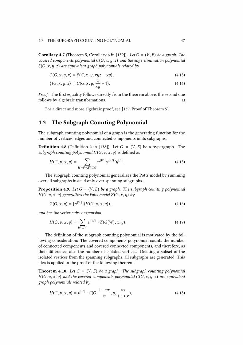
4.3. THE SUBGRAPH COUNTING POLYNOMIAL 47
Corollary 4.7 (Theorem 5, Corollary 6 in [139]). Let G = (V , E) be a graph. Thecovered components polynomial C (G , x ,y , z) and the edge elimination polynomialξ (G , x ,y , z) are equivalent graph polynomials related by
C (G , x ,y , z) = ξ (G , x ,y , xyz − xy), (4.13)
ξ (G , x ,y , z) = C (G , x ,y ,zxy
+ 1). (4.14)
Proof. The Vrst equality follows directly from the theorem above, the second onefollows by algebraic transformations. �
For a direct and more algebraic proof, see [139, Proof of Theorem 5].
4.3 The Subgraph Counting Polynomial
The subgraph counting polynomial of a graph is the generating function for thenumber of vertices, edges and connected components in its subgraphs.
DeVnition 4.8 (DeVnition 2 in [138]). Let G = (V , E) be a hypergraph. Thesubgraph counting polynomial H (G ,v , x ,y) is deVned as
H (G ,v , x ,y) =∑
H =(W,F )⊆G
v |W |xk (H )y |F | . (4.15)
The subgraph counting polynomial generalizes the Potts model by summingover all subgraphs instead only over spanning subgraphs.
Proposition 4.9. Let G = (V , E) be a graph. The subgraph counting polynomialH (G ,v , x ,y) generalizes the Potts model Z (G , x ,y) by
Z (G , x ,y) = [v |V |](H (G ,v , x ,y)), (4.16)
and has the vertex subset expansion
H (G ,v , x ,y) =∑
W ⊆V
v |W | · Z (G[W ], x ,y). (4.17)
The deVnition of the subgraph counting polynomial is motivated by the fol-lowing consideration: The covered components polynomial counts the numberof connected components and covered connected components, and therefore, astheir diUerence, also the number of isolated vertices. Deleting a subset of theisolated vertices from the spanning subgraphs, all subgraphs are generated. Thisidea is applied in the proof of the following theorem.
Theorem 4.10. Let G = (V , E) be a graph. The subgraph counting polynomialH (G ,v , x ,y) and the covered components polynomial C (G , x ,y , z) are equivalentgraph polynomials related by
H (G ,v , x ,y) = v |V | ·C (G ,1 +vxv,y ,
vx1 +vx
), (4.18)
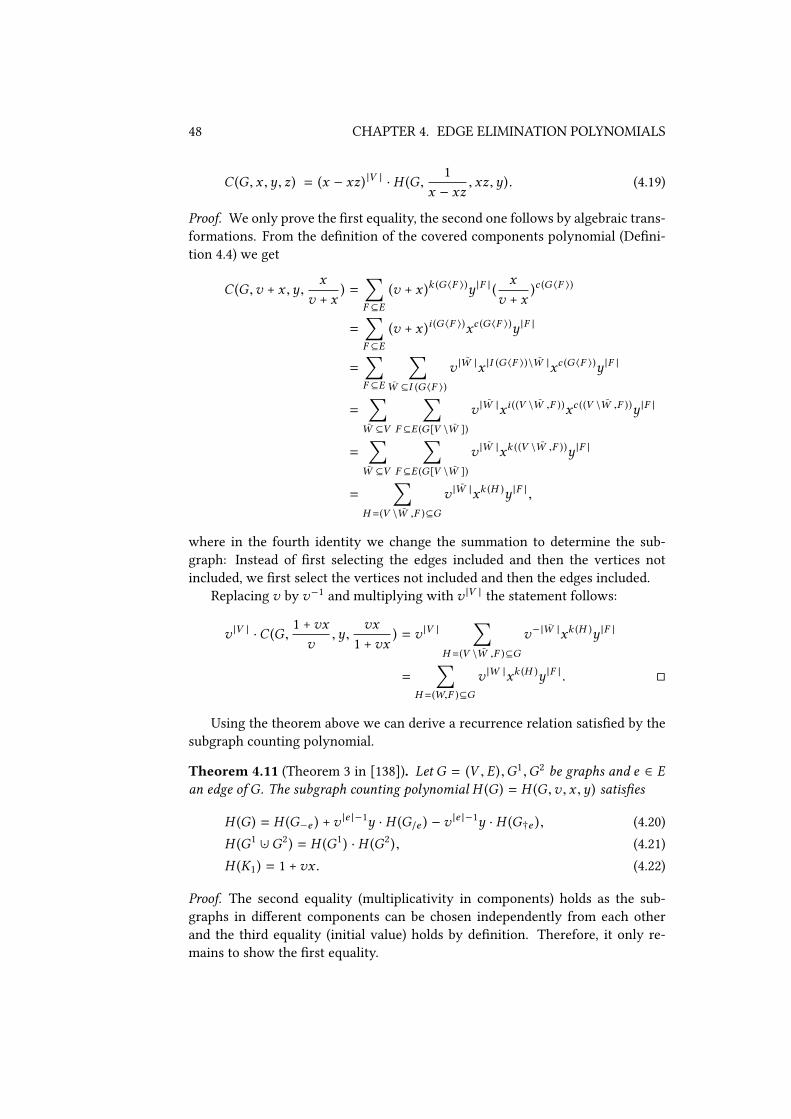
48 CHAPTER 4. EDGE ELIMINATION POLYNOMIALS
C (G , x ,y , z) = (x − xz) |V | · H (G ,1
x − xz, xz ,y). (4.19)
Proof. We only prove the Vrst equality, the second one follows by algebraic trans-formations. From the deVnition of the covered components polynomial (DeVni-tion 4.4) we get
C (G ,v + x ,y ,x
v + x) =
∑F ⊆E
(v + x )k (G 〈F 〉)y |F | (x
v + x)c (G 〈F 〉)
=∑F ⊆E
(v + x )i (G 〈F 〉)xc (G 〈F 〉)y |F |
=∑F ⊆E
∑W ⊆I (G 〈F 〉)
v |W |x |I (G 〈F 〉)\W |xc (G 〈F 〉)y |F |
=∑
W ⊆V
∑F ⊆E (G [V \W ])
v |W |xi ((V \W ,F ))xc ((V \W ,F ))y |F |
=∑
W ⊆V
∑F ⊆E (G [V \W ])
v |W |xk ((V \W ,F ))y |F |
=∑
H =(V \W ,F )⊆G
v |W |xk (H )y |F | ,
where in the fourth identity we change the summation to determine the sub-graph: Instead of Vrst selecting the edges included and then the vertices notincluded, we Vrst select the vertices not included and then the edges included.
Replacing v by v−1 and multiplying with v |V | the statement follows:
v |V | ·C (G ,1 +vxv,y ,
vx1 +vx
) = v |V |∑
H =(V \W ,F )⊆G
v−|W |xk (H )y |F |
=∑
H =(W,F )⊆G
v |W |xk (H )y |F | . �
Using the theorem above we can derive a recurrence relation satisVed by thesubgraph counting polynomial.
Theorem 4.11 (Theorem 3 in [138]). Let G = (V , E),G1 ,G2 be graphs and e ∈ Ean edge of G. The subgraph counting polynomial H (G ) = H (G ,v , x ,y) satisVes
H (G ) = H (G−e ) +v |e |−1y · H (G/e ) − v |e |−1y · H (G†e ), (4.20)
H (G1 ∪· G2) = H (G1) · H (G2), (4.21)
H (K1) = 1 +vx . (4.22)
Proof. The second equality (multiplicativity in components) holds as the sub-graphs in diUerent components can be chosen independently from each otherand the third equality (initial value) holds by deVnition. Therefore, it only re-mains to show the Vrst equality.

4.4. THE EXTENDED SUBGRAPH COUNTING POLYNOMIAL 49
Let H = H (G ,v , x ,y) = v−|V | · H (G ,v , x ,y) = C (G , 1+vxv ,y ,
vx1+vx ). From the
recurrence relation for the covered components polynomial (Theorem 4.6), weget
H (G ) = H (G−e ) + y · H (G/e ) −yv· H (G†e )
for an edge e ∈ E. For H (G ) = H (G ,v , x ,y), it follows
H (G ) = v |V | · H (G )
= v |V | ·[H (G−e ) + y · H (G/e ) −
yv· H (G†e )
]= v |V | · H (G−e ) +v |V |y · H (G/e ) − v |V |
yv· H (G†e )
= v |V (G−e ) | · H (G−e ) +v |e |−1yv |V (G/e ) | · H (G/e )
−v |e |−1yv |V (G†e ) | · H (G†e )
= H (G−e ) +v |e |−1y · H (G/e ) − v |e |−1y · H (G†e ). �
For a direct and more combinatorial proof, see [138, Proof of Theorem 3].
Corollary 4.12 (Corollary 4 in [138]). Let G = (V , E) be a graph. The sub-graph counting polynomial H (G ,v , x ,y) and the edge elimination polynomialξ (G , x ,y , z) are equivalent graph polynomials related by
H (G ,v , x ,y) = v |V | · ξ (G ,1 +vxv,y , −
yv
), (4.23)
ξ (G , x ,y , z) = (x − y) |V | · H (G ,1
x − y,y ,
zx − y
). (4.24)
Proof. The statements can be derived via the relations to the covered componentspolynomial (Corollary 4.7 and Theorem 4.10). �
Alternatively, the corollary above can be derived directly from the recurrencerelation, see [138, Proof of Corollary 4].
4.4 The Extended Subgraph Counting Polynomial
The extended subgraph counting polynomial of a graph is the generating func-tion for the number of vertices, edges, connected components and covered con-nected components in its subgraphs.
DeVnition 4.13. Let G = (V , E) be a hypergraph. The extended subgraph count-ing polynomial H ′(G ,v , x ,y , z) is deVned as
H ′(G ,v , x ,y , z) =∑
H =(W,F )⊆G
v |W |xk (H )y |F |zc (H ) . (4.25)
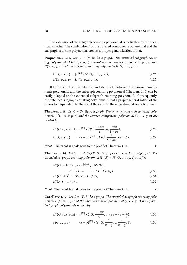
50 CHAPTER 4. EDGE ELIMINATION POLYNOMIALS
The extension of the subgraph counting polynomial is motivated by the ques-tion, whether “the combination” of the covered components polynomial and thesubgraph counting polynomial creates a proper generalization or not.
Proposition 4.14. Let G = (V , E) be a graph. The extended subgraph count-ing polynomial H ′(G ,v , x ,y , z) generalizes the covered components polynomialC (G , x ,y , z) and the subgraph counting polynomial H (G ,v , x ,y) by
C (G , x ,y , z) = [v |V |](H ′(G ,v , x ,y , z)) , (4.26)
H (G ,v , x ,y) = H ′(G ,v , x ,y , 1). (4.27)
It turns out, that the relation (and its proof) between the covered compo-nents polynomial and the subgraph counting polynomial (Theorem 4.10) can beeasily adapted to the extended subgraph counting polynomial. Consequently,the extended subgraph counting polynomial is not a proper generalization of theothers but equivalent to them and thus also to the edge elimination polynomial.
Theorem 4.15. Let G = (V , E) be a graph. The extended subgraph counting poly-nomial H ′(G ,v , x ,y , z) and the covered components polynomial C (G , x ,y , z) arerelated by
H ′(G ,v , x ,y , z) = v |V | ·C (G ,1 +vxv,y ,
vxz1 +vx
), (4.28)
C (G , x ,y , z) = (x − xz) |V | · H ′(G ,1
x − xz, xz ,y , 1). (4.29)
Proof. The proof is analogous to the proof of Theorem 4.10. �
Theorem 4.16. Let G = (V , E),G1 ,G2 be graphs and e ∈ E an edge of G. Theextended subgraph counting polynomial H ′(G ) = H ′(G ,v , x ,y , z) satisVes
H ′(G ) = H ′(G−e ) +v |e |−1y · H ′(G/e )
+v |e |−1y (vxz − vx − 1) · H ′(G†e ), (4.30)
H ′(G1 ∪· G2) = H ′(G1) · H ′(G2), (4.31)
H ′(K1) = 1 +vx . (4.32)
Proof. The proof is analogous to the proof of Theorem 4.11. �
Corollary 4.17. Let G = (V , E) be a graph. The extended subgraph counting poly-nomial H (G ,v , x ,y) and the edge elimination polynomial ξ (G , x ,y , z) are equiva-lent graph polynomials related by
H ′(G ,v , x ,y , z) = v |V | · ξ (G ,1 +vxv,y , xyz − xy −
yv
), (4.33)
ξ (G , x ,y , z) = (x − y) |V | · H ′(G ,1
x − y,y ,
zx − y
, 1). (4.34)
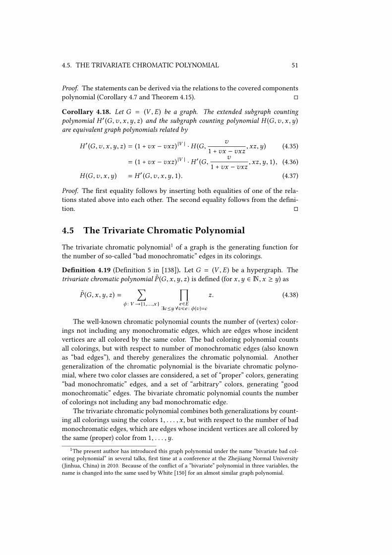
4.5. THE TRIVARIATE CHROMATIC POLYNOMIAL 51
Proof. The statements can be derived via the relations to the covered componentspolynomial (Corollary 4.7 and Theorem 4.15). �
Corollary 4.18. Let G = (V , E) be a graph. The extended subgraph countingpolynomial H ′(G ,v , x ,y , z) and the subgraph counting polynomial H (G ,v , x ,y)are equivalent graph polynomials related by
H ′(G ,v , x ,y , z) = (1 +vx − vxz) |V | · H (G ,v
1 +vx − vxz, xz ,y) (4.35)
= (1 +vx − vxz) |V | · H ′(G ,v
1 +vx − vxz, xz ,y , 1) , (4.36)
H (G ,v , x ,y) = H ′(G ,v , x ,y , 1). (4.37)
Proof. The Vrst equality follows by inserting both equalities of one of the rela-tions stated above into each other. The second equality follows from the deVni-tion. �
4.5 The Trivariate Chromatic Polynomial
The trivariate chromatic polynomial1 of a graph is the generating function forthe number of so-called “bad monochromatic” edges in its colorings.
DeVnition 4.19 (DeVnition 5 in [138]). Let G = (V , E) be a hypergraph. Thetrivariate chromatic polynomial P (G , x ,y , z) is deVned (for x ,y ∈ N, x ≥ y) as
P (G , x ,y , z) =∑
ϕ : V →{1,...,x }
∏e∈E
∃c≤y ∀v∈e : ϕ (v )=c
z. (4.38)
The well-known chromatic polynomial counts the number of (vertex) color-ings not including any monochromatic edges, which are edges whose incidentvertices are all colored by the same color. The bad coloring polynomial countsall colorings, but with respect to number of monochromatic edges (also knownas “bad edges”), and thereby generalizes the chromatic polynomial. Anothergeneralization of the chromatic polynomial is the bivariate chromatic polyno-mial, where two color classes are considered, a set of “proper” colors, generating“bad monochromatic” edges, and a set of “arbitrary” colors, generating “goodmonochromatic” edges. The bivariate chromatic polynomial counts the numberof colorings not including any bad monochromatic edge.
The trivariate chromatic polynomial combines both generalizations by count-ing all colorings using the colors 1, . . . , x , but with respect to the number of badmonochromatic edges, which are edges whose incident vertices are all colored bythe same (proper) color from 1, . . . ,y.
1The present author has introduced this graph polynomial under the name “bivariate bad col-oring polynomial” in several talks, Vrst time at a conference at the Zhejiiang Normal University(Jinhua, China) in 2010. Because of the conWict of a “bivariate” polynomial in three variables, thename is changed into the same used by White [150] for an almost similar graph polynomial.
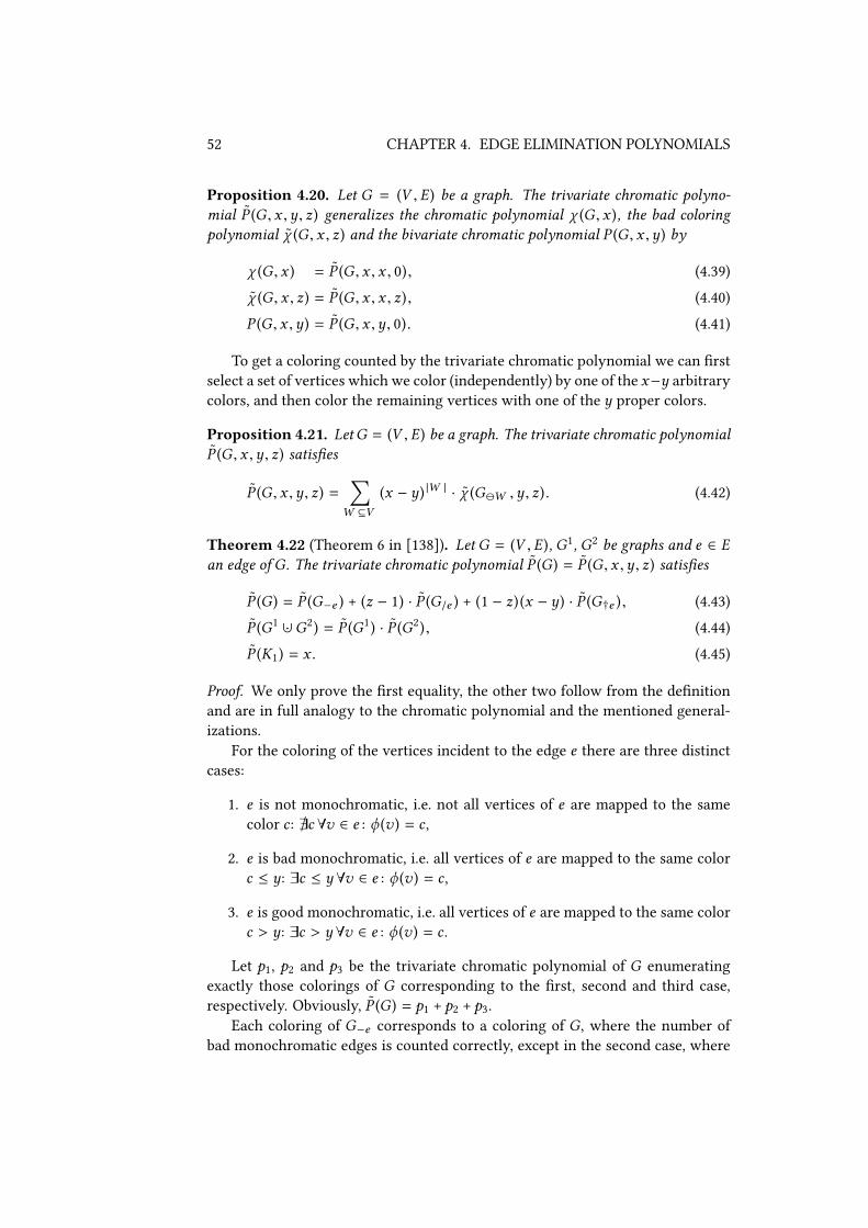
52 CHAPTER 4. EDGE ELIMINATION POLYNOMIALS
Proposition 4.20. Let G = (V , E) be a graph. The trivariate chromatic polyno-mial P (G , x ,y , z) generalizes the chromatic polynomial χ (G , x ), the bad coloringpolynomial χ (G , x , z) and the bivariate chromatic polynomial P (G , x ,y) by
χ (G , x ) = P (G , x , x , 0), (4.39)
χ (G , x , z) = P (G , x , x , z), (4.40)
P (G , x ,y) = P (G , x ,y , 0). (4.41)
To get a coloring counted by the trivariate chromatic polynomial we can Vrstselect a set of vertices which we color (independently) by one of the x−y arbitrarycolors, and then color the remaining vertices with one of the y proper colors.
Proposition 4.21. Let G = (V , E) be a graph. The trivariate chromatic polynomialP (G , x ,y , z) satisVes
P (G , x ,y , z) =∑
W ⊆V
(x − y) |W | · χ (GW ,y , z). (4.42)
Theorem 4.22 (Theorem 6 in [138]). Let G = (V , E), G1, G2 be graphs and e ∈ Ean edge of G. The trivariate chromatic polynomial P (G ) = P (G , x ,y , z) satisVes
P (G ) = P (G−e ) + (z − 1) · P (G/e ) + (1 − z) (x − y) · P (G†e ) , (4.43)
P (G1 ∪· G2) = P (G1) · P (G2), (4.44)
P (K1) = x . (4.45)
Proof. We only prove the Vrst equality, the other two follow from the deVnitionand are in full analogy to the chromatic polynomial and the mentioned general-izations.
For the coloring of the vertices incident to the edge e there are three distinctcases:
1. e is not monochromatic, i.e. not all vertices of e are mapped to the samecolor c: @c ∀v ∈ e : ϕ (v ) = c ,
2. e is bad monochromatic, i.e. all vertices of e are mapped to the same colorc ≤ y: ∃c ≤ y ∀v ∈ e : ϕ (v ) = c ,
3. e is good monochromatic, i.e. all vertices of e are mapped to the same colorc > y: ∃c > y ∀v ∈ e : ϕ (v ) = c .
Let p1, p2 and p3 be the trivariate chromatic polynomial of G enumeratingexactly those colorings of G corresponding to the Vrst, second and third case,respectively. Obviously, P (G ) = p1 + p2 + p3.
Each coloring of G−e corresponds to a coloring of G, where the number ofbad monochromatic edges is counted correctly, except in the second case, where
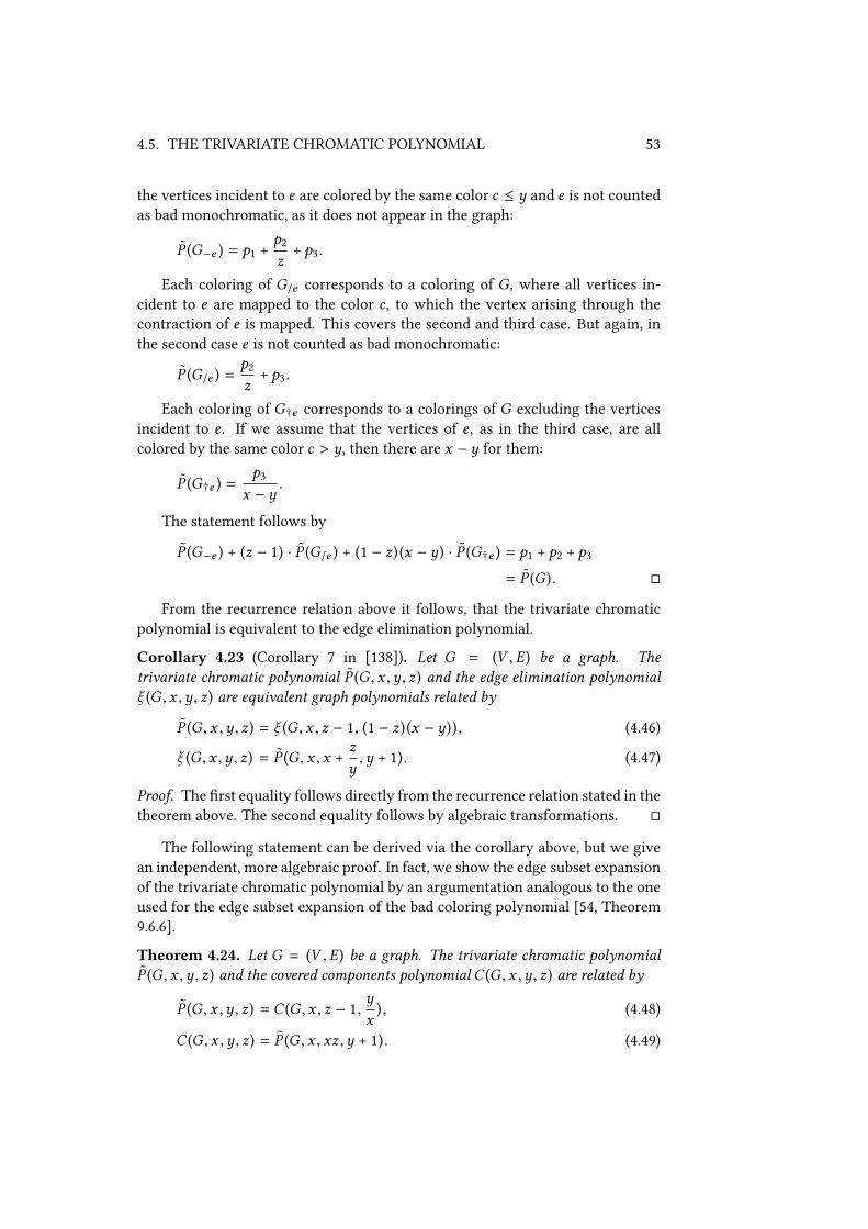
4.5. THE TRIVARIATE CHROMATIC POLYNOMIAL 53
the vertices incident to e are colored by the same color c ≤ y and e is not countedas bad monochromatic, as it does not appear in the graph:
P (G−e ) = p1 +p2
z+ p3.
Each coloring of G/e corresponds to a coloring of G, where all vertices in-cident to e are mapped to the color c , to which the vertex arising through thecontraction of e is mapped. This covers the second and third case. But again, inthe second case e is not counted as bad monochromatic:
P (G/e ) =p2
z+ p3.
Each coloring of G†e corresponds to a colorings of G excluding the verticesincident to e . If we assume that the vertices of e , as in the third case, are allcolored by the same color c > y, then there are x − y for them:
P (G†e ) =p3
x − y.
The statement follows by
P (G−e ) + (z − 1) · P (G/e ) + (1 − z) (x − y) · P (G†e ) = p1 + p2 + p3
= P (G ). �
From the recurrence relation above it follows, that the trivariate chromaticpolynomial is equivalent to the edge elimination polynomial.
Corollary 4.23 (Corollary 7 in [138]). Let G = (V , E) be a graph. Thetrivariate chromatic polynomial P (G , x ,y , z) and the edge elimination polynomialξ (G , x ,y , z) are equivalent graph polynomials related by
P (G , x ,y , z) = ξ (G , x , z − 1, (1 − z) (x − y)), (4.46)
ξ (G , x ,y , z) = P (G , x , x +zy,y + 1). (4.47)
Proof. The Vrst equality follows directly from the recurrence relation stated in thetheorem above. The second equality follows by algebraic transformations. �
The following statement can be derived via the corollary above, but we givean independent, more algebraic proof. In fact, we show the edge subset expansionof the trivariate chromatic polynomial by an argumentation analogous to the oneused for the edge subset expansion of the bad coloring polynomial [54, Theorem9.6.6].
Theorem 4.24. Let G = (V , E) be a graph. The trivariate chromatic polynomialP (G , x ,y , z) and the covered components polynomial C (G , x ,y , z) are related by
P (G , x ,y , z) = C (G , x , z − 1,yx
), (4.48)
C (G , x ,y , z) = P (G , x , xz ,y + 1). (4.49)
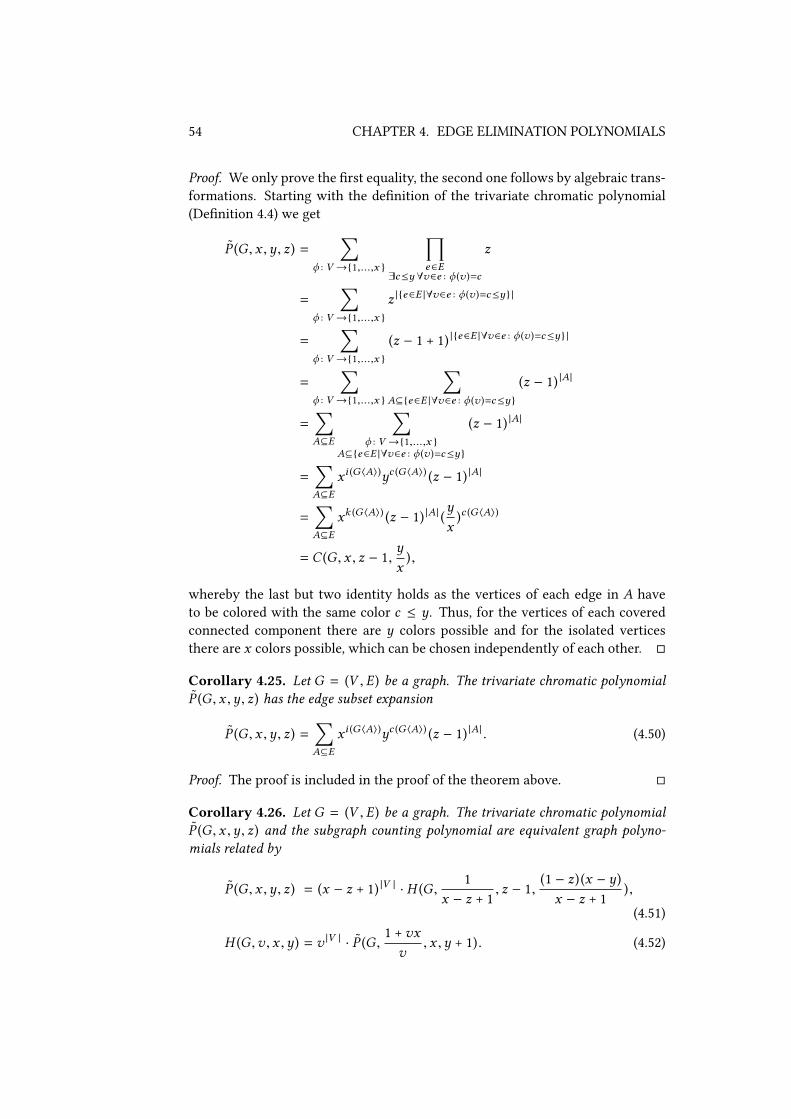
54 CHAPTER 4. EDGE ELIMINATION POLYNOMIALS
Proof. We only prove the Vrst equality, the second one follows by algebraic trans-formations. Starting with the deVnition of the trivariate chromatic polynomial(DeVnition 4.4) we get
P (G , x ,y , z) =∑
ϕ : V →{1,...,x }
∏e∈E
∃c≤y ∀v∈e : ϕ (v )=c
z
=∑
ϕ : V →{1,...,x }
z | {e∈E |∀v∈e : ϕ (v )=c≤y} |
=∑
ϕ : V →{1,...,x }
(z − 1 + 1) | {e∈E |∀v∈e : ϕ (v )=c≤y} |
=∑
ϕ : V →{1,...,x }
∑A⊆{e∈E |∀v∈e : ϕ (v )=c≤y}
(z − 1) |A|
=∑A⊆E
∑ϕ : V →{1,...,x }
A⊆{e∈E |∀v∈e : ϕ (v )=c≤y}
(z − 1) |A|
=∑A⊆E
xi (G 〈A〉)yc (G 〈A〉) (z − 1) |A|
=∑A⊆E
xk (G 〈A〉) (z − 1) |A| (yx
)c (G 〈A〉)
= C (G , x , z − 1,yx
),
whereby the last but two identity holds as the vertices of each edge in A haveto be colored with the same color c ≤ y. Thus, for the vertices of each coveredconnected component there are y colors possible and for the isolated verticesthere are x colors possible, which can be chosen independently of each other. �
Corollary 4.25. Let G = (V , E) be a graph. The trivariate chromatic polynomialP (G , x ,y , z) has the edge subset expansion
P (G , x ,y , z) =∑A⊆E
xi (G 〈A〉)yc (G 〈A〉) (z − 1) |A| . (4.50)
Proof. The proof is included in the proof of the theorem above. �
Corollary 4.26. Let G = (V , E) be a graph. The trivariate chromatic polynomialP (G , x ,y , z) and the subgraph counting polynomial are equivalent graph polyno-mials related by
P (G , x ,y , z) = (x − z + 1) |V | · H (G ,1
x − z + 1, z − 1,
(1 − z) (x − y)x − z + 1
),
(4.51)
H (G ,v , x ,y) = v |V | · P (G ,1 +vxv, x ,y + 1). (4.52)

4.6. FURTHER EDGE ELIMINATION POLYNOMIALS 55
Proof. The statements can be derived via the relations to the edge eliminationpolynomial (Corollary 4.12 and Corollary 4.23). �
The trivariate chromatic polynomial and its recurrence relation given aboveare utilized by Garijo, Goodall and Nešetřil [59, Theorem 34] to prove that theedge elimination polynomial can be stated as counting graph homomorphisms.
Theorem 4.27 (Theorem 34 in [59]). Let G = (V , E) be a graph. The trivariatechromatic polynomial P (G , x ,y , z) equals (for x ,y , z ∈ N, x ≥ y) the number ofhomomorphisms of G into K1
x−y + Kzy , where K
zn is the complete graph of n vertices
with z loops attached at each vertex and the graph K1x−y +Kz
y arises from the join ofa K1
x−y and a Kzy ,
P (G , x ,y , z) = hom(G ,K1x−y + Kz
y ). (4.53)
4.6 Further Edge Elimination Polynomials
In this section we mention some other graph polynomials equivalent to the edgeelimination polynomial, which are given in the literature.
4.6.1 The Hyperedge Elimination Polynomial
The hyperedge elimination polynomial ξ (G , x ,y , z) has been introduced byWhite [150, Section 4] as an (explicit) “hyperedge version” of the edge eliminationpolynomial. It is deVned [150, DeVnition 1] by an identity similar to the expan-sion of the edge elimination polynomial in terms of 3-partitions of the edge set[4, Theorem 5] (Theorem 4.3), which instead of the number of covered connectedcomponents of a spanning subgraph uses the number of connected componentsin the edge-induced subgraph.
DeVnition 4.28 (DeVnition 1 in [150]). Let G = (V , E) be a hypergraph. Thehyperedge elimination polynomial ξ (G , x ,y , z) is deVned as
ξ (G , x ,y , z) =∑
(AtB)⊆E
xk (G 〈A∪B〉)−k (G [B])y |A|+|B |−k (G [B])zk (G [B]) , (4.54)
where (A t B) ⊆ E is used for the summation over pairs of edge subsets(A, B) : A, B ⊆ E, such that the set of vertices incident to the edges of A and Bare disjoint:
⋃e∈A e ∩
⋃e∈B e = ∅.
White [150, Proposition 1] shows that the hyperedge elimination polynomialsatisVes exactly the same recurrence relation that are used to deVne the edgeelimination polynomial (DeVnition 4.1).

56 CHAPTER 4. EDGE ELIMINATION POLYNOMIALS
4.6.2 The Subgraph Enumerating Polynomial
The Vrst graph polynomial deVned that is equivalent to the edge eliminationpolynomial, is in fact not the edge elimination polynomial itself, but the sub-graph enumerating polynomial deVned by Borzacchini and Pulito more than twodecades ago.
DeVnition 4.29 (Equation (1) in [29]). Let G = (V , E) be a graph. The subgraphenumerating polynomial P (G ,u ,v ,p) is deVned as
P (G ,u ,v ,p) =∑A⊆E
ui (G 〈A〉)v |A|pk (G 〈A〉) , (4.55)
where i (G ) is the number of non-isolated vertices in G.
Furthermore, the authors also proved a recurrence relation with respect tothe usual three edge elimination operations.
Theorem 4.30 (Theorem 2 in [29]). Let G = (V , E),G1 ,G2 be graphs and e ∈ Ean edge of G. The subgraph enumerating polynomial P (G ) = P (G ,u ,v ,p) satisVes
P (G ) = P (G−e ) + u |e |−1v · P (G/e ) + u |e |−1 (u − 1)vp · P (G†e ), (4.56)
P (G1 ∪· G2) = P (G1) · P (G2), (4.57)
P (K1) = p. (4.58)
The subgraph enumerating polynomial is strongly related to the coveredcomponents polynomial, both diUer only in the usage of the number of non-isolated vertices and covered connected components, respectively.
Theorem 4.31. Let G = (V , E) be a graph. The subgraph enumerating polynomialP (G ,u ,v ,p) and the covered components polynomial C (G , x ,y , z) are equivalentgraph polynomials related by
P (G ,u ,v ,p) = u |V | ·C (G ,pu,v ,u), (4.59)
C (G , x ,y , z) = z−|V | · P (G , z ,y , xz). (4.60)
Proof. The Vrst equality follows from
P (G ,u ,v ,p) =∑A⊆E
ui (G 〈A〉)v |A|pk (G 〈A〉)
=∑A⊆E
u |V |−k (G 〈A〉)+c (G 〈A〉)v |A|pk (G 〈A〉)
= u |V | ·∑A⊆E
(pu
)k (G 〈A〉) v |A| uc (G 〈A〉)
= u |V | ·C (G ,pu,v ,u),
and the second one by algebraic transformations. �
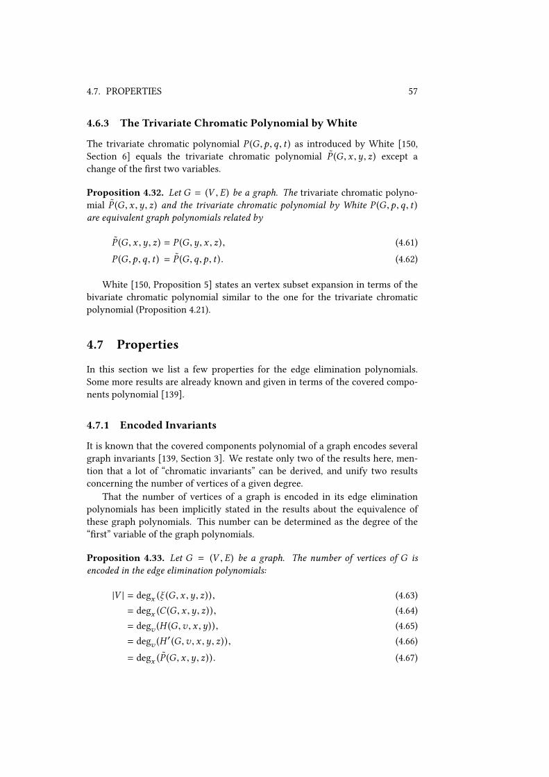
4.7. PROPERTIES 57
4.6.3 The Trivariate Chromatic Polynomial by White
The trivariate chromatic polynomial P (G ,p ,q, t ) as introduced by White [150,Section 6] equals the trivariate chromatic polynomial P (G , x ,y , z) except achange of the Vrst two variables.
Proposition 4.32. Let G = (V , E) be a graph. The trivariate chromatic polyno-mial P (G , x ,y , z) and the trivariate chromatic polynomial by White P (G ,p ,q, t )are equivalent graph polynomials related by
P (G , x ,y , z) = P (G ,y , x , z), (4.61)
P (G ,p ,q, t ) = P (G ,q,p , t ). (4.62)
White [150, Proposition 5] states an vertex subset expansion in terms of thebivariate chromatic polynomial similar to the one for the trivariate chromaticpolynomial (Proposition 4.21).
4.7 Properties
In this section we list a few properties for the edge elimination polynomials.Some more results are already known and given in terms of the covered compo-nents polynomial [139].
4.7.1 Encoded Invariants
It is known that the covered components polynomial of a graph encodes severalgraph invariants [139, Section 3]. We restate only two of the results here, men-tion that a lot of “chromatic invariants” can be derived, and unify two resultsconcerning the number of vertices of a given degree.
That the number of vertices of a graph is encoded in its edge eliminationpolynomials has been implicitly stated in the results about the equivalence ofthese graph polynomials. This number can be determined as the degree of the“Vrst” variable of the graph polynomials.
Proposition 4.33. Let G = (V , E) be a graph. The number of vertices of G isencoded in the edge elimination polynomials:
|V | = degx (ξ (G , x ,y , z)), (4.63)
= degx (C (G , x ,y , z)), (4.64)
= degv (H (G ,v , x ,y)), (4.65)
= degv (H ′(G ,v , x ,y , z)) , (4.66)
= degx (P (G , x ,y , z)). (4.67)

58 CHAPTER 4. EDGE ELIMINATION POLYNOMIALS
One graph invariant that is not included in many graph polynomials is thenumber of edge-induced subgraphs with given number of vertices, edges and con-nected components. This number can be derived from the covered componentspolynomial [139, Theorem 16], but a generalization can be easily obtained fromthe coeXcients of the extended subgraph counting polynomial.
Proposition 4.34. Let G = (V , E) be a graph. The number of subgraphs withexactly n vertices, m edges, k connected components, c of them covered connectedcomponents, denoted by д(n,m, k , c ), is given as a coeXcient of the extended sub-graph counting polynomial H ′(G ,v , x ,y , z):
д(n,m, k , c ) = [vnxkymzc ](H ′(G ,v , x ,y , z)). (4.68)
From the trivariate chromatic polynomial many chromatic invariants can bedetermined. Beside the usual chromatic number, that is the minimal number ofcolors necessary for a proper coloring of the vertices, also some extensions upto the number of colors necessary for a partial coloring with a given number ofmonochromatic edges.
Proposition 4.35. Let G = (V , E) be a graph. The minimal number of colorsnecessary for a coloring of all but a vertices such that b edges are monochromatic,denoted by χa,b (G ), is encoded in the trivariate chromatic polynomial P (G , x ,y , z):
χa,b (G ) = min {x ∈ N | [vazb](P (v + x , x , z)) > 0)}. (4.69)
There are already two results concerning the encoding of the number of ver-tices with a given degree: First, the number of vertices of degree 0, 1 and ofminimum degree can be determined from the covered components polynomial[139, Section 3]. Second, the number of vertices of a given degree in a forestis encoded in the edge elimination polynomial [139, Theorem 36] (shown by aproof using the recurrence relation). Using the trivariate chromatic polynomialboth results can be uniVed.
Theorem 4.36 (Theorem 11 in [138]). Let G = (V , E) be a graph. The numberof vertices with degree i in G, deg−1 (G , i ), is encoded in the trivariate chromaticpolynomial P (G , x ,y , z):
deg−1 (G , i ) = [v1z |E |−i ](P (G ,v + 1, 1, z)), (4.70)
where |E | = degz (P (G ,v + 1, 1, z)).
Informal this can be shown as follows: We consider the number of badmonochromatic edges in a coloring using v arbitrary and 1 proper color. Eachterm including v1 corresponds to colorings where exactly one vertex is coloredby one of the v arbitrary colors and all other vertices are colored by the sameproper color. Hence, all edges except the edges incident to the one arbitrary col-ored vertex are bad monochromatic, and their number is counted in the variablez.

4.7. PROPERTIES 59
For a proof following this argumentation, see [138, Theorem 11]. Here wegive a slightly diUerent proof using the edge subset expansion of the trivariatechromatic polynomial.
Proof. Applying the edge subset expansion of the trivariate chromatic polynomial(Corollary 4.25),
P (G , x ,y , z) =∑A⊆E
xi (G 〈A〉)yc (G 〈A〉) (z − 1) |A| ,
for P (G ,v + 1, 1, z), it follows
P (G ,v + 1, 1, z) =∑A⊆E
(v + 1)i (G 〈A〉)1c (G 〈A〉) (z − 1) |A|
=∑A⊆E
(v + 1) |I (G 〈A〉) | (z − 1) |A|
=∑A⊆E
∑W ⊆I (G 〈A〉)
v |W | (z − 1) |A|
=∑
W ⊆V
∑A⊆E (GW )
v |W | (z − 1) |A|
=∑
W ⊆V
v |W |∑
A⊆E (GW )
(z − 1) |A|
=∑
W ⊆V
v |W |z |E (GW ) | .
Consequently, the coeXcient in front of the monomial v1z |E |−i counts the num-ber of vertices, whose deletion removes i edges, and hence the number of verticeswith degree i in G, deg−1 (G , i ). �
4.7.2 Derivatives
The following theorem is analogous to a statement given for the subgraph enu-merating polynomial [29, Theorem 4].
Theorem 4.37. Let G = (V , E) be a graph. The subgraph counting polynomialH (G ,v , x ,y) satisVes
|V | · H (G ,v , x ,y) =∑v∈V
H (Gv ,v , x ,y) +v∂H (G ,v , x ,y)
∂v. (4.71)
Proof. The subgraph counting polynomial H (G ,v , x ,y) enumerates the numberof vertices, edges and connected components in the subgraphs of G, i.e.
H (G ,v , x ,y) =∑i,j,k
h(G , i , j , k )vix jyk ,

60 CHAPTER 4. EDGE ELIMINATION POLYNOMIALS
where h(G , i , j , k ) is the number of subgraphs of G with i vertices, j edges and kconnected components.
By Kelly’s Lemma [85], each subgraph with exactly i vertices is a subgraph of|V | − i vertex-deleted subgraphs (with one of the |V | − i missing vertices deleted),i.e. for all i , j , k we have
( |V | − i ) · h(G , i , j , k ) =∑v∈V
h(Gv , i , j , k ).
Hence,
( |V | − i )∑i,j,k
h(G , i , j , k )vix jyk =∑v∈V
∑i,j,k
h(Gv , i , j , k )vix jyk .
Using the deVnition of the subgraph counting polynomial and the identity
i∑i,j,k
h(G , i , j , k )vix jyk = v∂∑i,j,k h(G , i , j , k )vix jyk
∂v,
the statement follows:
|V | · H (G ,v , x ,y) =∑v∈V
H (Gv ,v , x ,y) +v∂H (G ,v , x ,y)
∂v. �
4.7.3 Reconstructability
Kotek [89, Theorem 2.5] has shown that the edge elimination polynomial of asimple graph with at least three vertices is reconstructable from the isomorphismclasses of its deck.
This is also possible without having exactly (the isomorphism classes of) thegraphs in the deck. It is enough to know the corresponding incidence matrixN (G ), deVned by Thatte [133], which represents how often any induced sub-graph of G is induced in any other.
Corollary 4.38. Let G = (V , E) be a simple graph with at least three vertices. Thecovered components polynomial C (G , x ,y , z) is reconstructable from the incidencematrix N (G ).
Proof. The statement follows directly from [133, Lemma 3.14] by the same ar-gument used for the rank polynomial in [133, Lemma 3.15]: From N (G ) the“number of subgraphs with v vertices (none of which isolated), e edges and l[connected] components”, and hence all coeXcients of the covered componentspolynomial can be determined. �
For the polynomial reconstructability, the probably Vrst aXrmative statementin this direction is given by Tutte for the rank polynomial [142; 143].
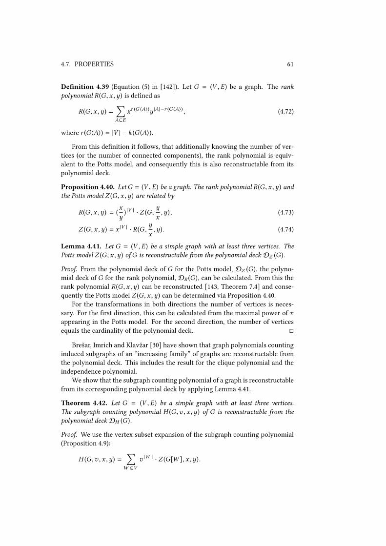
4.7. PROPERTIES 61
DeVnition 4.39 (Equation (5) in [142]). Let G = (V , E) be a graph. The rankpolynomial R (G , x ,y) is deVned as
R (G , x ,y) =∑A⊆E
xr (G 〈A〉)y |A|−r (G 〈A〉) , (4.72)
where r (G〈A〉) = |V | − k (G〈A〉).
From this deVnition it follows, that additionally knowing the number of ver-tices (or the number of connected components), the rank polynomial is equiv-alent to the Potts model, and consequently this is also reconstructable from itspolynomial deck.
Proposition 4.40. Let G = (V , E) be a graph. The rank polynomial R (G , x ,y) andthe Potts model Z (G , x ,y) are related by
R (G , x ,y) = (xy
) |V | · Z (G ,yx,y), (4.73)
Z (G , x ,y) = x |V | · R (G ,yx,y). (4.74)
Lemma 4.41. Let G = (V , E) be a simple graph with at least three vertices. ThePotts model Z (G , x ,y) of G is reconstructable from the polynomial deck DZ (G ).
Proof. From the polynomial deck of G for the Potts model, DZ (G ), the polyno-mial deck of G for the rank polynomial, DR (G ), can be calculated. From this therank polynomial R (G , x ,y) can be reconstructed [143, Theorem 7.4] and conse-quently the Potts model Z (G , x ,y) can be determined via Proposition 4.40.
For the transformations in both directions the number of vertices is neces-sary. For the Vrst direction, this can be calculated from the maximal power of xappearing in the Potts model. For the second direction, the number of verticesequals the cardinality of the polynomial deck. �
Brešar, Imrich and Klavžar [30] have shown that graph polynomials countinginduced subgraphs of an “increasing family” of graphs are reconstructable fromthe polynomial deck. This includes the result for the clique polynomial and theindependence polynomial.
We show that the subgraph counting polynomial of a graph is reconstructablefrom its corresponding polynomial deck by applying Lemma 4.41.
Theorem 4.42. Let G = (V , E) be a simple graph with at least three vertices.The subgraph counting polynomial H (G ,v , x ,y) of G is reconstructable from thepolynomial deck DH (G ).
Proof. We use the vertex subset expansion of the subgraph counting polynomial(Proposition 4.9):
H (G ,v , x ,y) =∑
W ⊆V
v |W | · Z (G[W ], x ,y).
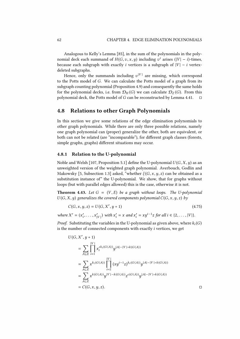
62 CHAPTER 4. EDGE ELIMINATION POLYNOMIALS
Analogous to Kelly’s Lemma [85], in the sum of the polynomials in the poly-nomial deck each summand of H (G ,v , x ,y) including vi arises ( |V | − i )-times,because each subgraph with exactly i vertices is a subgraph of |V | − i vertex-deleted subgraphs.
Hence, only the summands including v |V | are missing, which correspondto the Potts model of G. We can calculate the Potts model of a graph from itssubgraph counting polynomial (Proposition 4.9) and consequently the same holdsfor the polynomial decks, i.e. from DH (G ) we can calculate DZ (G ). From thispolynomial deck, the Potts model of G can be reconstructed by Lemma 4.41. �
4.8 Relations to other Graph Polynomials
In this section we give some relations of the edge elimination polynomials toother graph polynomials. While there are only three possible relations, namelyone graph polynomial can (proper) generalize the other, both are equivalent, orboth can not be related (are “incomparable”), for diUerent graph classes (forests,simple graphs, graphs) diUerent situations may occur.
4.8.1 Relation to the U-polynomial
Noble and Welsh [107, Proposition 5.1] deVne the U-polynomialU (G ,X ,y) as anunweighted version of the weighted graph polynomial. Averbouch, Godlin andMakowsky [5, Subsection 1.3] asked, “whether ξ (G , x ,y , z) can be obtained as asubstitution instance of” the U-polynomial. We show, that for graphs withoutloops (but with parallel edges allowed) this is the case, otherwise it is not.
Theorem 4.43. Let G = (V , E) be a graph without loops. The U-polynomialU (G ,X ,y) generalizes the covered components polynomial C (G , x ,y , z) by
C (G , x ,y , z) = U (G ,X ′,y + 1) (4.75)
where X ′ = (x ′1 , . . . , x′|V | ) with x
′1 = x and x ′i = xyi−1z for all i ∈ {2, . . . , |V |}.
Proof. Substituting the variables in the U-polynomial as given above, where ki (G )is the number of connected components with exactly i vertices, we get
U (G ,X ′,y + 1)
=∑A⊆E
|V |∏i=1
x ′iki (G 〈A〉)y |A|− |V |+k (G 〈A〉)
=∑A⊆E
xk1 (G 〈A〉)|V |∏i=2
(xyi−1z)ki (G 〈A〉)y |A|− |V |+k (G 〈A〉)
=∑A⊆E
xk (G 〈A〉)y |V |−k (G 〈A〉)zc (G 〈A〉)y |A|− |V |+k (G 〈A〉)
= C (G , x ,y , z). �
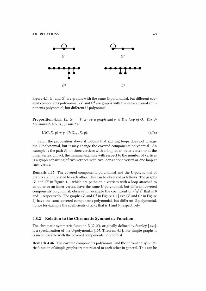
4.8. RELATIONS 63
G1 G2
G3 G4
Figure 4.1: G1 and G2 are graphs with the same U-polynomial, but diUerent cov-ered components polynomial, G3 and G4 are graphs with the same covered com-ponents polynomial, but diUerent U-polynomial.
Proposition 4.44. Let G = (V , E) be a graph and e ∈ E a loop of G. The U-polynomial U (G ,X ,y) satisVes
U (G ,X ,y) = y ·U (G−e ,X ,y). (4.76)
From the proposition above it follows that shifting loops does not changethe U-polynomial, but it may change the covered components polynomial. Anexample is the path P3 on three vertices with a loop at an outer vertex or at theinner vertex. In fact, the minimal example with respect to the number of verticesis a graph consisting of two vertices with two loops at one vertex or one loop ateach vertex.
Remark 4.45. The covered components polynomial and the U-polynomial ofgraphs are not related to each other. This can be observed as follows: The graphsG1 and G2 in Figure 4.1, which are paths on 3 vertices with a loop attached toan outer or an inner vertex, have the same U-polynomial, but diUerent coveredcomponents polynomial, observe for example the coeXcient of x2y2z2 that is 0and 1, respectively. The graphs G3 and G4 in Figure 4.1 [139, G5 and G6 in Figure2] have the same covered components polynomial, but diUerent U-polynomial,notice for example the coeXcients of x4x6 that is 1 and 0, respectively.
4.8.2 Relation to the Chromatic Symmetric Function
The chromatic symmetric function X (G ,X ), originally deVned by Stanley [130],is a specialization of the U-polynomial [107, Theorem 6.1]. For simple graphs itis incomparable with the covered components polynomial.
Remark 4.46. The covered components polynomial and the chromatic symmet-ric function of simple graphs are not related to each other in general. This can be

64 CHAPTER 4. EDGE ELIMINATION POLYNOMIALS
G5 G6
G7 G8
Figure 4.2: G5 and G6 are graphs with the same chromatic symmetric function,but diUerent covered components polynomial, G7 and G8 are graphs with thesame covered components polynomial, but diUerent chromatic symmetric func-tion.
observed as follows: The graphs G5 and G6 in Figure 4.2 [130, G and H in Figure1] have the same chromatic symmetric function, but diUerent covered compo-nents polynomial, notice for example the coeXcient of x2y5z. The graphs G7 andG8 in Figure 4.2 [139, G5 and G6 in Figure 2] have the same covered componentspolynomial, but diUerent chromatic symmetric function, because all trees withat most 23 vertices have a unique chromatic symmetric function [101, Section 0,due to Tan].
The situation changes if only trees are considered.
Remark 4.47. The chromatic symmetric function generalizes the covered com-ponents polynomial of trees. This can be concluded from the relations of bothpolynomials to the U-polynomial: For trees, the chromatic symmetric function isequivalent to the U-polynomial (“[107, Theorem 6.1] is easily seen to be reversiblefor trees” [101, Section 0]), and the U-polynomial generalizes the covered compo-nents polynomial (Theorem 4.43).
4.8.3 Relation to the Subgraph Component Polynomial
The subgraph component polynomial Q (G , x ,y) is the generating function forthe number of vertices and connected components in the induced subgraphs.
It is known that the subgraph component polynomial of the line graph L(G )can be derived from the edge elimination polynomial of G [134, Theorem 23].We show that for forests the subgraph counting polynomial and the subgraphcomponent polynomial are equivalent to each other.
Theorem 4.48 (Theorem 8 in [138]). Let G = (V , E) be a forest. The sub-graph counting polynomial H (G ,v , x ,y) and the subgraph component polynomial

4.8. RELATIONS 65
Q (G ,v , x ) are equivalent graph polynomials related by
H (G ,v , x ,y) = Q (G ,v (x + y),x
x + y), (4.77)
Q (G ,v , x ) = H (G ,v , x , 1 − x ). (4.78)
Proof. We start with the vertex subset expansion of the subgraph counting poly-nomial in terms of the Potts model (Proposition 4.9). The Potts model of a forestdepends only on the number of vertices and the number of connected compo-nents (each edge reduces the number of connected components by one), hencewe have
H (G ,v , x ,y) =∑
W ⊆V
v |W | · Z (G[W ], x ,y)
=∑
W ⊆V
v |W |xk (G [W ]) (x + y) |W |−k (G [W ]) .
Then the Vrst equality follows by
Q (G ,v (x + y),x
x + y) =
∑W ⊆V
(v (x + y)) |W |(
xx + y
)k (G [W ])
=∑
W ⊆V
v |W |xk (G [W ]) (x + y) |W |−k (G [W ])
= H (G ,v , x ,y),
and the second equality follows by
H (G ,v , x , 1 − x ) =∑
W ⊆V
v |W |xk (G [W ]) (1) |V |−k (G [W ])
=∑
W ⊆V
v |W |xk (G [W ])
= Q (G ,v , x ). �
Remark 4.49. The subgraph component polynomial and the subgraph countingpolynomial of simple graphs are not related to each other. This can be observedas follows: The graphs G9 and G10 in Figure 4.3 [139, G3 and G4 in Figure 2]have the same subgraph counting polynomial, but diUerent subgraph componentpolynomial, notice for example the coeXcient of v6x1. The graphs G11 and G12
in Figure 4.3 [7, G7 and G8 in Figure 1] have the same subgraph component poly-nomial, but diUerent chromatic polynomial and hence diUerent subgraph count-ing polynomial. (For non-simple graphs this follows already from the fact thatthe subgraph component polynomial does not consider parallel edges and loops,which the subgraph counting polynomial does.)
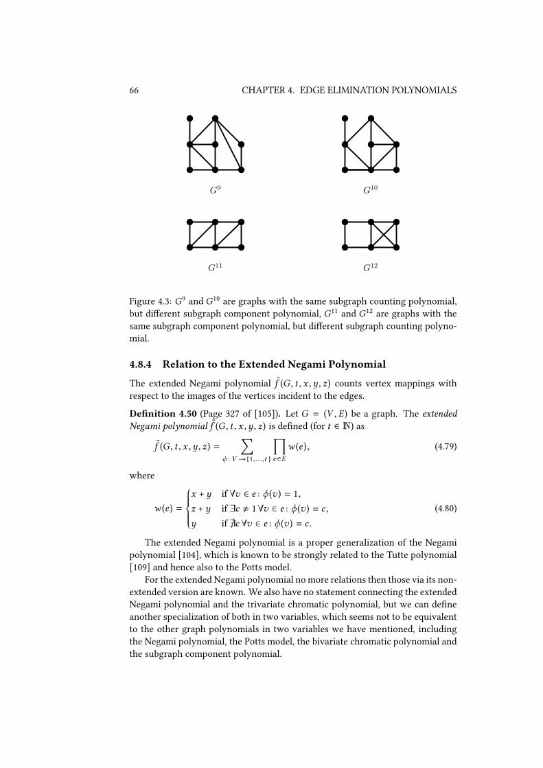
66 CHAPTER 4. EDGE ELIMINATION POLYNOMIALS
G9 G10
G11 G12
Figure 4.3: G9 and G10 are graphs with the same subgraph counting polynomial,but diUerent subgraph component polynomial, G11 and G12 are graphs with thesame subgraph component polynomial, but diUerent subgraph counting polyno-mial.
4.8.4 Relation to the Extended Negami Polynomial
The extended Negami polynomial f (G , t , x ,y , z) counts vertex mappings withrespect to the images of the vertices incident to the edges.
DeVnition 4.50 (Page 327 of [105]). Let G = (V , E) be a graph. The extendedNegami polynomial f (G , t , x ,y , z) is deVned (for t ∈ N) as
f (G , t , x ,y , z) =∑
ϕ : V →{1,...,t }
∏e∈E
w (e ), (4.79)
where
w (e ) =
x + y if ∀v ∈ e : ϕ (v ) = 1,
z + y if ∃c , 1∀v ∈ e : ϕ (v ) = c ,y if @c ∀v ∈ e : ϕ (v ) = c .
(4.80)
The extended Negami polynomial is a proper generalization of the Negamipolynomial [104], which is known to be strongly related to the Tutte polynomial[109] and hence also to the Potts model.
For the extended Negami polynomial no more relations then those via its non-extended version are known. We also have no statement connecting the extendedNegami polynomial and the trivariate chromatic polynomial, but we can deVneanother specialization of both in two variables, which seems not to be equivalentto the other graph polynomials in two variables we have mentioned, includingthe Negami polynomial, the Potts model, the bivariate chromatic polynomial andthe subgraph component polynomial.

4.8. RELATIONS 67
Theorem 4.51. Let G = (V , E) be a graph. There are specializations of thetrivariate chromatic polynomial P (G , x ,y , z) and the extended Negami polynomialf (G , t , x ,y , z) that equal each other:
P (G , x , x − 1, z) = f (G , x , 0, 1, z − 1) (4.81)
Proof. The trivariate chromatic polynomial can be stated as
P (G , x ,y , z) =∑
ϕ : V →{1,...,x }
∏e∈E
w (e ),
where
w (e ) =
z if ∃c ≤ y ∀v ∈ e : ϕ (v ) = c ,1 else.
Consequently, for P (G , x , x − 1, z) the function w (e ) changes to
w (e ) =
z if ∃c ≤ x − 1∀v ∈ e : ϕ (v ) = c ,1 else,
which equals the corresponding function for f (G , x , 0, 1, z − 1) (with exceptionthat the colors / states are renamed). �
4.8.5 Relation to the Bivariate Chromatic Polynomial
By Proposition 4.20, the bivariate chromatic polynomial is a specialization ofthe trivariate chromatic polynomial, and for forests both are equivalent. This isshown by the present author for the covered components polynomial [139, The-orem 38]. Here we show the equivalence of the bivariate and trivariate chromaticpolynomial more directly by making use of the fact that for forests the numberof edges is determined by the number of vertices and the number of connectedcomponents.
Theorem 4.52. Let G = (V , E) be a forest. The trivariate chromatic polynomialP (G , x ,y , z) and the bivariate chromatic polynomial P (G , x ,y , z) are equivalentgraph polynomials related by
P (G , x ,y , z) = (1 − z)−|V | · P (G ,x
1 − z,
y1 − z
), (4.82)
P (G , x ,y) = P (G , x ,y , 0). (4.83)
Proof. Using the edge subset expansions of both polynomials (Corollary 4.25), thestatement follows by
P (G , x ,y , z) =∑A⊆E
xi (G 〈A〉)yc (G 〈A〉) (z − 1) |A|

68 CHAPTER 4. EDGE ELIMINATION POLYNOMIALS
G13 G14
Figure 4.4: G13 andG14 are graphs with the same bivariate chromatic polynomial,but diUerent trivariate chromatic polynomial.
=∑A⊆E
xi (G 〈A〉)yc (G 〈A〉) (1 − z) |V |−k (G 〈A〉) (−1) |A|
= (1 − z)−|V |∑A⊆E
( x1 − z
)i (G 〈A〉) ( y1 − z
)c (G 〈A〉)(−1) |A|
= (1 − z)−|V | · P (G ,x
1 − z,
y1 − z
). �
Remark 4.53. The trivariate chromatic polynomial properly generalizes the bi-variate chromatic polynomial of simple graphs. This can be concluded from thegraphsG13 andG14 in Figure 4.4 [139,G1 andG2 in Figure 1], which have the samebivariate chromatic polynomial, but diUerent covered components polynomials,observe for example the number of vertices of degree 4.
4.8.6 Relation to the Wiener Polynomial
The Wiener polynomial W (G , x ) is the generating function for the distance oftwo vertices.
DeVnition 4.54 (Equation 1 of [120]). Let G = (V , E) be a connected graph. TheWiener polynomialW (G ,q) is deVned as
W (G ,q) =∑
{u,v }∈(V2 )
qd (G,u,v ) , (4.84)
where d (G ,u ,v ) is the distance of the vertices u and v in G.
Remark 4.55. The covered components polynomial and the Wiener polynomialof simple graphs are not related to each other. This can be observed as follows:The graphs G15 and G16 in Figure 4.5, which are a cycle on 4 vertices and a cycleon 3 vertices with an additional pendent edge, have the same Wiener polynomial(2 pairs of vertices of distance 2, all other pairs have distance 1), but diUerent cov-ered components polynomial, observe for example that the coeXcient of x2y3z1
is 0 and 1, respectively. The graphs G17 and G18 in Figure 4.5 [139, G5 and G6 inFigure 2] have the same covered components polynomial, but diUerent Wienerpolynomial, notice for example thatG12 has two vertices of distance 7, whichG11
does not have.

4.8. RELATIONS 69
G15 G16
G17 G18
Figure 4.5: G15 andG16 are graphs with the same Wiener polynomial, but diUerentcovered components polynomial, G17 and G18 are graphs with the same coveredcomponents polynomial, but diUerent Wiener polynomial.

70 CHAPTER 4. EDGE ELIMINATION POLYNOMIALS

Chapter 5
The Generalized SubgraphCounting Polynomial —A Unifying Graph Polynomial
The edge elimination polynomial and the subgraph component polynomial are“most general graph polynomials” with respect to recurrence relations using dele-tion, contraction and extraction of an edge [4, Theorem 3], and deletion, neigh-borhood deletion and contraction of a vertex [134, Theorem 22], respectively.That means that every graph polynomial satisfying such recurrence relation canbe calculated from them.
In Section 5.1 we deVne the generalized subgraph counting polynomial, aunifying graph polynomial in the sense that it generalizes both the edge elimi-nation polynomial (by generalizing the subgraph counting polynomial) and thesubgraph component polynomial. As main result of this chapter we prove a re-currence relation of the newly introduced graph polynomial applicable for hy-pergraphs.
Some relations to other graph polynomials and some properties are given inSection 5.2 and Section 5.3, respectively. In the last we give some evidence, whythe generalized subgraph counting polynomial probably is not “a most generalgraph polynomial” with respect to the recurrence relation satisVed by itself.
While most of the deVnitions and statements in this chapter are given forgraphs, many of them are also valid in the case of hypergraphs. For this, it maybe necessary to generalize known graph polynomials to hypergraphs, their deV-nitions are given accordingly in Appendix A.
5.1 DeVnition and Recurrence Relation
The generalized subgraph counting polynomial extends the subgraph countingpolynomial by additional counting the number of edges in the subgraphs inducedby the vertex set of the considered subgraph.
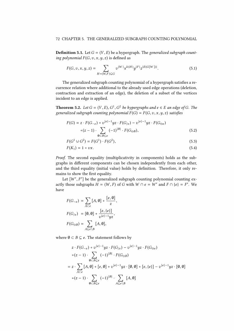
72 CHAPTER 5. THE GENERALIZED SUBGRAPH COUNTING POLYNOMIAL
DeVnition 5.1. LetG = (V , E) be a hypergraph. The generalized subgraph count-ing polynomial F (G ,v , x ,y , z) is deVned as
F (G ,v , x ,y , z) =∑
H =(W,F )⊆G
v |W |xk (H )y |F |z |E (G [W ]) | . (5.1)
The generalized subgraph counting polynomial of a hypergraph satisVes a re-currence relation where additional to the already used edge operations (deletion,contraction and extraction of an edge), the deletion of a subset of the verticesincident to an edge is applied.
Theorem 5.2. Let G = (V , E),G1 ,G2 be hypergraphs and e ∈ E an edge of G. Thegeneralized subgraph counting polynomial F (G ) = F (G ,v , x ,y , z) satisVes
F (G ) = z · F (G−e ) +v |e |−1yz · F (G/e ) − v |e |−1yz · F (Ge )
+(z − 1) ·∑∅⊂B⊆e
(−1) |B | · F (GB ), (5.2)
F (G1 ∪· G2) = F (G1) · F (G2), (5.3)
F (K1) = 1 +vx . (5.4)
Proof. The second equality (multiplicativity in components) holds as the sub-graphs in diUerent components can be chosen independently from each other,and the third equality (initial value) holds by deVnition. Therefore, it only re-mains to show the Vrst equality.
Let [W ′, F ′] be the generalized subgraph counting polynomial counting ex-actly those subgraphs H = (W , F ) of G with W ∩ e =W ′ and F ∩ {e} = F ′. Wehave
F (G−e ) =∑A⊂e
[A, ∅] +[e , ∅]z,
F (G/e ) = [∅, ∅] +[e , {e}]v |e |−1yz
,
F (GB ) =∑
A⊆e\B
[A, ∅],
where ∅ ⊂ B ⊆ e . The statement follows by
z · F (G−e ) +v |e |−1yz · F (G/e ) − v |e |−1yz · F (Ge )
+(z − 1) ·∑∅⊂B⊆e
(−1) |B | · F (GB )
= z ·∑A⊂e
[A, ∅] + [e , ∅] +v |e |−1yz · [∅, ∅] + [e , {e}] − v |e |−1yz · [∅, ∅]
+(z − 1) ·∑∅⊂B⊆e
(−1) |B | ·∑
A⊆e\B
[A, ∅]
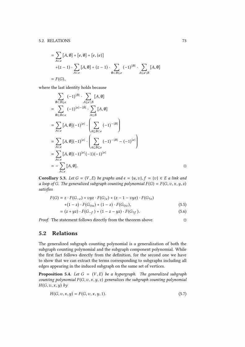
5.2. RELATIONS 73
=∑A⊂e
[A, ∅] + [e , ∅] + [e , {e}]
+(z − 1) ·∑A⊂e
[A, ∅] + (z − 1) ·∑∅⊂B⊆e
(−1) |B | ·∑
A⊆e\B
[A, ∅]
= F (G ),
where the last identity holds because∑∅⊂B⊆e
(−1) |B | ·∑
A⊆e\B
[A, ∅]
=∑∅⊆B⊂e
(−1) |e |− |B | ·∑A⊆B
[A, ∅]
=∑A⊂e
[A, ∅](−1) |e | ·
∑A⊆B⊂e
(−1)−|B |
=∑A⊂e
[A, ∅](−1) |e | ·
∑A⊆B⊆e
(−1)−|B | − (−1) |e |
=∑A⊂e
[A, ∅](−1) |e | (−1)(−1) |e |
= −∑A⊂e
[A, ∅]. �
Corollary 5.3. Let G = (V , E) be graphs and e = {u ,v}, f = {v} ∈ E a link anda loop of G. The generalized subgraph counting polynomial F (G ) = F (G ,v , x ,y , z)satisVes
F (G ) = z · F (G−e ) +vyz · F (G/e ) + (z − 1 − vyz) · F (G†e )
+(1 − z) · F (Gu ) + (1 − z) · F (Gv ), (5.5)
= (z + yz) · F (G−f ) + (1 − z − yz) · F (G†f ). (5.6)
Proof. The statement follows directly from the theorem above. �
5.2 Relations
The generalized subgraph counting polynomial is a generalization of both thesubgraph counting polynomial and the subgraph component polynomial. Whilethe Vrst fact follows directly from the deVnition, for the second one we haveto show that we can extract the terms corresponding to subgraphs including alledges appearing in the induced subgraph on the same set of vertices.
Proposition 5.4. Let G = (V , E) be a hypergraph. The generalized subgraphcounting polynomial F (G ,v , x ,y , z) generalizes the subgraph counting polynomialH (G ,v , x ,y) by
H (G ,v , x ,y) = F (G ,v , x ,y , 1). (5.7)
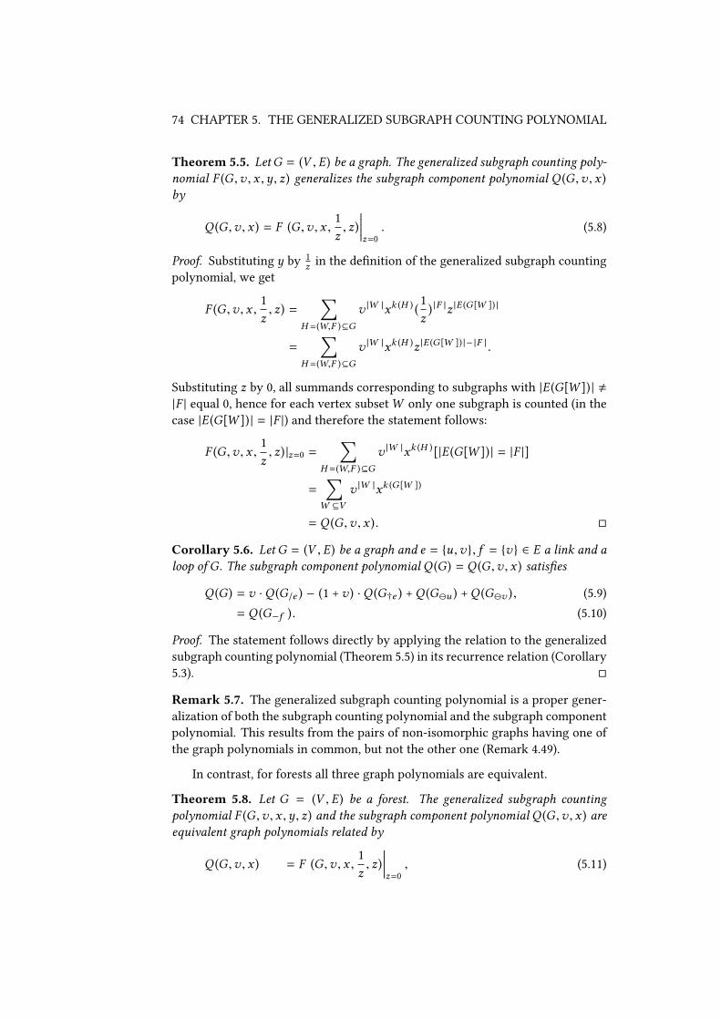
74 CHAPTER 5. THE GENERALIZED SUBGRAPH COUNTING POLYNOMIAL
Theorem 5.5. Let G = (V , E) be a graph. The generalized subgraph counting poly-nomial F (G ,v , x ,y , z) generalizes the subgraph component polynomial Q (G ,v , x )by
Q (G ,v , x ) = F (G ,v , x ,1z, z)
∣∣∣∣∣z=0. (5.8)
Proof. Substituting y by 1z in the deVnition of the generalized subgraph counting
polynomial, we get
F (G ,v , x ,1z, z) =
∑H =(W,F )⊆G
v |W |xk (H ) (1z
) |F |z |E (G [W ]) |
=∑
H =(W,F )⊆G
v |W |xk (H )z |E (G [W ]) |− |F | .
Substituting z by 0, all summands corresponding to subgraphs with |E (G[W ]) | ,|F | equal 0, hence for each vertex subsetW only one subgraph is counted (in thecase |E (G[W ]) | = |F |) and therefore the statement follows:
F (G ,v , x ,1z, z) |z=0 =
∑H =(W,F )⊆G
v |W |xk (H )[|E (G[W ]) | = |F |]
=∑
W ⊆V
v |W |xk (G [W ])
= Q (G ,v , x ). �
Corollary 5.6. Let G = (V , E) be a graph and e = {u ,v}, f = {v} ∈ E a link and aloop of G. The subgraph component polynomial Q (G ) = Q (G ,v , x ) satisVes
Q (G ) = v ·Q (G/e ) − (1 +v ) ·Q (G†e ) +Q (Gu ) +Q (Gv ), (5.9)
= Q (G−f ). (5.10)
Proof. The statement follows directly by applying the relation to the generalizedsubgraph counting polynomial (Theorem 5.5) in its recurrence relation (Corollary5.3). �
Remark 5.7. The generalized subgraph counting polynomial is a proper gener-alization of both the subgraph counting polynomial and the subgraph componentpolynomial. This results from the pairs of non-isomorphic graphs having one ofthe graph polynomials in common, but not the other one (Remark 4.49).
In contrast, for forests all three graph polynomials are equivalent.
Theorem 5.8. Let G = (V , E) be a forest. The generalized subgraph countingpolynomial F (G ,v , x ,y , z) and the subgraph component polynomial Q (G ,v , x ) areequivalent graph polynomials related by
Q (G ,v , x ) = F (G ,v , x ,1z, z)
∣∣∣∣∣z=0, (5.11)
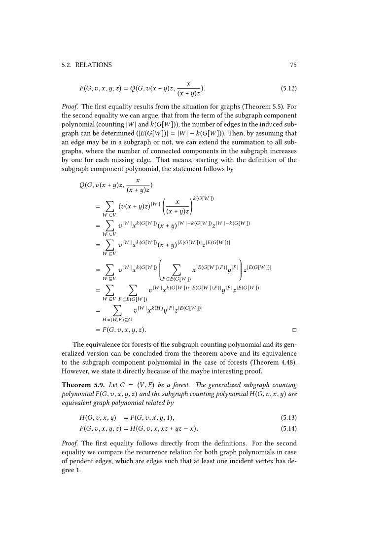
5.2. RELATIONS 75
F (G ,v , x ,y , z) = Q (G ,v (x + y)z ,x
(x + y)z). (5.12)
Proof. The Vrst equality results from the situation for graphs (Theorem 5.5). Forthe second equality we can argue, that from the term of the subgraph componentpolynomial (counting |W | and k (G[W ])), the number of edges in the induced sub-graph can be determined (|E (G[W ]) | = |W | − k (G[W ])). Then, by assuming thatan edge may be in a subgraph or not, we can extend the summation to all sub-graphs, where the number of connected components in the subgraph increasesby one for each missing edge. That means, starting with the deVnition of thesubgraph component polynomial, the statement follows by
Q (G ,v (x + y)z ,x
(x + y)z)
=∑
W ⊆V
(v (x + y)z) |W |(
x(x + y)z
)k (G [W ])
=∑
W ⊆V
v |W |xk (G [W ]) (x + y) |W |−k (G [W ])z |W |−k (G [W ])
=∑
W ⊆V
v |W |xk (G [W ]) (x + y) |E (G [W ]) |z |E (G [W ]) |
=∑
W ⊆V
v |W |xk (G [W ])
∑F ⊆E (G [W ])
x |E (G [W ]\F ) |y |F | z |E (G [W ]) |
=∑
W ⊆V
∑F ⊆E (G [W ])
v |W |xk (G [W ])+|E (G [W ]\F ) |y |F |z |E (G [W ]) |
=∑
H =(W,F )⊆G
v |W |xk (H )y |F |z |E (G [W ]) |
= F (G ,v , x ,y , z). �
The equivalence for forests of the subgraph counting polynomial and its gen-eralized version can be concluded from the theorem above and its equivalenceto the subgraph component polynomial in the case of forests (Theorem 4.48).However, we state it directly because of the maybe interesting proof.
Theorem 5.9. Let G = (V , E) be a forest. The generalized subgraph countingpolynomial F (G ,v , x ,y , z) and the subgraph counting polynomial H (G ,v , x ,y) areequivalent graph polynomial related by
H (G ,v , x ,y) = F (G ,v , x ,y , 1), (5.13)
F (G ,v , x ,y , z) = H (G ,v , x , xz + yz − x ). (5.14)
Proof. The Vrst equality follows directly from the deVnitions. For the secondequality we compare the recurrence relation for both graph polynomials in caseof pendent edges, which are edges such that at least one incident vertex has de-gree 1.
76 CHAPTER 5. THE GENERALIZED SUBGRAPH COUNTING POLYNOMIAL
Because each non-empty forest has at least one pendent edge, a graph poly-nomial of a forest can be calculated recursively by a recurrence relation for pen-dent edges (together with the multiplicativity with respect to components and aninitial value).
Let e = {u ,v} ∈ E be a pendent edge of G with deg(G ,u) = 1. From therecurrence relation for the generalized subgraph counting polynomial F (G ) =F (G ,v , x ,y , z) of an arbitrary edge (Theorem 5.2) we get
F (G ) = z · F (G−e ) +vyz · F (G/e ) + (z − 1 − vyz) · F (G†e )
+(1 − z) · F (Gu ) + (1 − z) · F (Gv )
= z (1 +vx ) · F (Gu ) +vyz · F (Gu ) + (z − 1 − vyz) · F (Guv )
+(1 − z) · F (Gu ) + (1 − z) (1 +vx ) · F (Gv )
= [vxz +vyz + 1] · F (Gu ) + [vx − vxz − vyz] · F (Guv ),
and for H (G ) = H (G ,v , x ,y) = F (G ,v , x ,y , 1) it follows
H (G ) = [vx +vy + 1] · H (Gu ) + [−vy] · H (Guv ).
Therefore, H (G ,v , x , xz +yz − x ) and F (G ,v , x ,y , z) satisfy the same recurrencerelation and consequently the second equality holds. �
In the literature there is another graph polynomial generalizing both the edgeelimination polynomial and the subgraph component polynomial, the homomor-phism polynomial H (G , k , x ,y , z) [59, page 1044] deVned by Garijo, Goodall andNešetřil. It is deVned as the number of homomorphisms from G to the graphHk,x,y,z , H (G , k , x ,y , z) = hom(G ,Hk,x,y,z ), where Hk,x,y,z is the join of a Kz
k withthe disjoint union of y copies of Kz
x , where Kln is a complete graph on n vertices
with l loops attached at each vertex. The authors give a vertex subset expansionof the graph polynomial in terms of the Potts models of induced graphs, whichcan be rewritten such that the diUerence to the generalized subgraph countingpolynomial becomes more clear.
Proposition 5.10 (Page 1044 in [59]). Let G = (V , E) be a graph. The homomor-phism polynomial h(G , k , x ,y , z) satisVes
h(G , k , x ,y , z) =∑
W ⊆V
k |V |− |W |yk (G [W ])P (G[W ], x , z) (5.15)
=∑
H =(W,F )⊆G
k |V |− |W |yk (G [W ])xk (H )z |F | . (5.16)
Therefore, in addition to renaming variables, the diUerence between the gen-eralized subgraph counting polynomial and the homomorphism polynomial isthat the Vrst counts the edges and the second counts the connected componentsin the subgraph induced by the vertex set of the considered subgraph.
But this fact gives no straightforward insight into the relation of both graphpolynomials and hence this is an open problem (Question 6).
5.3. PROPERTIES 77
5.3 Properties
5.3.1 Polynomial Reconstructability
The generalized subgraph counting polynomial of a graph is reconstructable fromits polynomial deck by the same line of arguments valid for the non-generalizedversion (Theorem 4.42), caused by a similar vertex subset expansion as a sumover Potts models.
Proposition 5.11. Let G = (V , E) be a graph. The generalized subgraph countingpolynomial F (G ,v , x ,y , z) generalizes the Potts model Z (G , x ,y) by
Z (G , x ,y) = [v |V |](F (G ,v , x ,y , 1)), (5.17)
and has the vertex subset expansion
F (G ,v , x ,y , z) =∑
W ⊆V
v |W |z |E (G [W ]) | · Z (G[W ], x ,y). (5.18)
Theorem 5.12. Let G = (V , E) be a simple graph with at least three vertices. Thegeneralized subgraph counting polynomial F (G ,v , x ,y , z) of G is reconstructablefrom the polynomial deck DF (G ).
Proof. We use the vertex subset expansion of the generalized subgraph countingpolynomial (Proposition 5.11):
F (G ,v , x ,y , z) =∑
W ⊆V
v |W |z |E (G [W ]) | · Z (G[W ], x ,y).
Analogous to Kelly’s Lemma [85], in the sum of the polynomials in the poly-nomial deck each summand of F (G ,v , x ,y , z) including vi arises ( |V | − i )-times,because each subgraph with exactly i vertices is a subgraph of |V | − i vertex-deleted subgraphs.
Hence, only the summands including v |V | are missing, which correspond tothe Potts model of G (the factor z |E | can be determined as degy (Z (G , x ,y))). Wecan calculate the Potts model of a graph from its extended subgraph countingpolynomial (Proposition 5.11) and consequently the same holds for the polyno-mial decks, i.e. fromDF (G ) we can calculateDZ (G ). From this polynomial deck,the Potts model of G can be reconstructed by Lemma 4.41. �
5.3.2 Non-isomorphic Graphs with Coinciding Generalized Sub-graph Counting Polynomial
We have already shown that the generalized subgraph counting polynomial isa proper generalization of the subgraph counting polynomial and the subgraphcomponent polynomial. This can also be seen from the fact that the last two donot distinguish all simple graphs with 8 vertices, which is done by the Vrst.

78 CHAPTER 5. THE GENERALIZED SUBGRAPH COUNTING POLYNOMIAL
G19 G20
Figure 5.1: G19 and G20 are two non-isomorphic graphs with the same extendedsubgraph counting polynomial.
Remark 5.13. The generalized subgraph counting polynomial distinguishes sim-ple graphs with less than 9 vertices. The graphs G19 and G20 of Figure 5.1 are theminimal non-isomorphic graphs (minimal with respect to the number of vertices)with the same generalized subgraph counting polynomial.
For forests, all three mentioned graph polynomials are equivalent (Theorem5.8 and Theorem 5.9). Therefore, the pairs of non-isomorphic trees with the samecovered components polynomial have also the same generalized subgraph count-ing polynomial. For all those pairs with up to 12 vertices, see [139, Figure 2 andFigure 3].
5.3.3 Not Necessarily a “Most General” Graph Polynomial
The edge elimination polynomial and the subgraph counting polynomial are themost general graph polynomials with respect to those graph polynomials satisfy-ing a similar recurrence relation. However, it seems unlikely that the same holdsfor the generalized subgraph counting polynomial.
DeVnition 5.14. Let G = (V , E),G1 ,G2 be a graphs and e = {u ,v}, f ={w } ∈ E a link and a loop of G. The (non-invariant) graph polynomial Ξ(G ) =Ξ(G , α , β ,γ , δ , ϵ , ζ , x ) is deVned by
Ξ(G ) = α · Ξ(G−e ) + β · Ξ(G/e ) + γ · Ξ(G†e ) (5.19)
+δ · Ξ(Gu ) + δ · Ξ(Gv ), (5.20)
Ξ(G ) = ϵ · Ξ(G−f ) + ζ · Ξ(G†f ), (5.21)
Ξ(En ) = xn . (5.22)
We determine suXcient conditions of the parameters α , . . . , ζ , such that thegraph polynomial Ξ(G ) is an invariant.
Remark 5.15. We have already assumed that the coeXcients of Ξ(Gu ) andΞ(Gv ) are equal (here δ ), because this is obviously a necessary condition for aninvariant graph polynomial.

5.3. PROPERTIES 79
G1
e f
G2
e f
G3
e f
G4
u
v
w
e f
G5
u
v
e f
G6
e f
G7
e f
Figure 5.2: DiUerent cases for the elimination of two edges e and f .
By Theorem 3.16 it follows that the graph polynomial Ξ(G ) is multiplicativein components.
We have to determine under which conditions the application of the re-currence relation for two edges is interchangeable. This approach and alsothe following analysis are analogous to those given by Averbouch, Godlin andMakowsky [3, Section 3.3; 4, Section 2].
Theorem 5.16. The graph polynomial Ξ(G , α , β ,γ , δ , ϵ , ζ ) is an invariant graphpolynomial if the following equations are satisVed:
(α − 1)γ = (β + δ )δ , (5.23)
(α − 1)ζ = δ (ϵ − 1), (5.24)
(β + δ )ζ = γ (ϵ − 1). (5.25)
Proof. We have to check all situations of the mutual location of two edges, eitherthese are two links, a link and a loop, or two loops. The cases are displayed inFigure 5.2.
Let EF i be Ξ(Gi ) calculated by eliminating Vrst the edge e and second theedge f and let FEi be Ξ(Gi ) calculated by eliminating Vrst the edge f and secondthe edge e . The conditions must be determined, under which the arising graphpolynomial is independent of the order of the elimination of the edges e and f , i.e. EF i = FEi = 0 for i = 1, . . . , 7.
If the two edges have no common vertex, as in the graphs G1, G2 and G3, orare symmetrically, as in the graphs G6 and G7, the graphs occurring and theirprefactors do not depend on the order of the operated edge. Hence, the resultingpolynomials EF i and FEi are identical for i = 1, 2, 3, 6, 7.
80 CHAPTER 5. THE GENERALIZED SUBGRAPH COUNTING POLYNOMIAL
It remains to check the cases for i = 4, 5, where we write Gs instead of Ξ(Gs )for the sake of brevity.
The graph G4 contains the edges e = {u ,v} and f = {v ,w }. We have
EF 4 = α ·G−e + β ·G/e + γ ·G†e + δ ·Gu + δ ·Gv= α · [α ·G−e−f + β ·G−e/f + γ ·G−e†f + δ ·G−ev + δ ·G−ew ]
+ β · [α ·G/e−f + β ·G/e/f + γ ·G/e†f + δ ·G/ev + δ ·G/ew ]
+ γ ·G†e+ δ · [α ·Gu−f + β ·Gu/f + γ ·Gu†f + δ ·Guv + δ ·Guw ]
+ δ ·Gv
and
FE4 = α ·G−f + β ·G/f + γ ·G†f + δ ·Gv + δ ·Gw= α · [α ·G−f −e + β ·G−f/e + γ ·G−f †e + δ ·G−f u + δ ·G−f v]
+ β · [α ·G/f −e + β ·G/f/e + γ ·G/f †e + δ ·G/f u + δ ·G/f v]
+ γ ·G†f+ δ ·Gv+ δ · [α ·Gw−e + β ·Gw/e + γ ·Gw†e + δ ·Gwu + δ ·Gwv].
Using the commutativity of the following operations
G−e−f = G−f −e , G−e/f = G/f −e , G−ew = Gw−e ,
G/e−f = G−f/e , G/e/f = G/f/e , G/ew = Gw/e ,
Gu−f = G−f u , Gu/f = G/f u , Guw = Gwu ,
and the following identities
Gv = G−ev = G−f v ,
Guv = G/ev = G†e = G−f †e ,
Gvw = G−e†f = G†f = Gvw ,
Guvw = G/e†f = G/f †e = Gu†f = Gw†e ,
we get as a necessary condition for a graph invariant that
EF4 − FE4 = (Guv −Gvw ) · (−αγ + βδ + γ + δ 2) = 0,
which equals
(α − 1)γ = (β + δ )δ . (5.26)
The graph G5 contains the edges e = {u ,v} and f = {v}. We have
EF 5 = α ·G−e + β ·G/e + γ ·G†e + δ ·Gu + δ ·Gv
5.3. PROPERTIES 81
= α · [ϵ ·G−e−f + ζ ·G−e†f ]
+ β · [ϵ ·G/e−f + ζ ·G/e†f ]
+ γ ·G†e+ δ · [ϵ ·Gu−f + ζ ·Gu†f ]
+ δ ·Gv
and
FE5 = ϵ ·G−f + ζ ·G†f= ϵ · [α ·G−f −e + β ·G−f/e + γ ·G−f †e + δ ·G−f u + δ ·G−f v]
+ ζ ·G†f .
Using the commutativity of the following operations
G−e−f = G−f −e , G−e/f = G/f −e , G/e−f = G−f/e ,
G/e/f = G/f/e , Gu−f = G−f u , Gu/f = G/f u ,
and the following identities
Gv = G−e†f = G†f = G−ev = G−f v ,
Guv = G/ev = G†e = G−f †e = Gu†f = G/e†f = G/f †e ,
we get as a necessary condition for a graph invariant that
EF5 − FE5 = Guv · (βζ + γ + δζ − ϵγ )
+ Gv · (αζ + δ − δϵ − ζ ) = 0,
which equals
(α − 1)ζ = δ (ϵ − 1),
(β + δ )ζ = γ (ϵ − 1). �
The edge elimination polynomial corresponds to the case δ = 0, ϵ = α + βand ζ = γ . Thereby, the second equation is fulVlled and the third one equals theVrst one. The Vrst equation has in fact two diUerent solutions, α = 1 and γ = 0.Hence, to show that this graph polynomial is “a most general” one satisfying suchkind of recurrence relation, it has been necessary to argument that the case α = 1is more general than γ = 0. This holds, because the second case is equivalent tothe Potts model [4, Equation 21].
While the generalized subgraph counting polynomial also satisVes the equa-tions given in the theorem above, there are much more solutions for them.Whether each of these solutions is a specialization of or equivalent to the gener-alized subgraph counting polynomial is an open problem (Question 7), but at leastit seems to be unlikely. Therefore, to attack this problem, it seems appropriateto look for solutions corresponding to graph polynomials distinguishing non-isomorphic graphs with the same generalized subgraph counting polynomial, forexample G1 and G2 in Figure 5.1.
82 CHAPTER 5. THE GENERALIZED SUBGRAPH COUNTING POLYNOMIAL
Chapter 6
Conclusion
The aim of this dissertation is to make some progress to a better understandingof graph polynomials and their relations. This is done by
• collecting several concepts used to deVne graph polynomials and statingrelations between them (Chapter 3),
• introducing graph polynomials equivalent to the edge elimination poly-nomial and thereby linking a graph polynomial deVned by a recurrencerelation to the counting of (spanning) subgraphs and colorings (Chapter 4),
• deVning a graph polynomial that uniVes several of the well-known graphpolynomials (Chapter 5).
We think some evidence is given that the investigation of equivalent graphpolynomials can be very useful, although or rather because these are mathemat-ically the same.
We have restricted our investigation to graph polynomials associated to hy-pergraphs with a constant number of variables. Therefore, neither graph poly-nomials associated to other graph-like structures, for example directed graphs,graph embeddings and knots, nor multivariate graph polynomials, where usu-ally a variable for each vertex or edge is used, are considered here. Furthermore,the topic of this thesis has been concentrated on graph polynomials that can bedeVned by or satisfy a recurrence relation.
For sure, this sole work can not cover all topics related to graph polynomials,not even with the mentioned restrictions. But it seems that graph polynomials geta lot of attention in the last years, especially from PhD students. Hence, togetherwith the theses of Averbouch [3], Csikvari [43] and HoUmann [78], whose topicsare all mostly mutually disjoint, there has been some progress “towards a generaltheory of graph polynomials” [100].
In the following Section 6.1 we present graphically our current knowledgeabout the relations between some graph polynomials. Some open problems men-tioning unknown relations and other questions for further research are given inSection 6.2.

84 CHAPTER 6. CONCLUSION
6.1 An Overview about Graph Polynomials
We summarize the most of our knowledge about the relations between diUerentgraph polynomials in Figure 6.1. There we display a “graph of graph polynomi-als”, where the vertices represent graph polynomials and where an directed edgefrom graph polynomial A to graph polynomial B means that B can be calculatedfrom A in the case of graphs.
Please note the following remarks for the dashed edges:
• the relation from the U-polynomial to the covered components polynomialholds only for simple graphs,
• for the calculation of the Potts model and the Negami polynomial from theTutte polynomial, the number of vertices is necessary.
6.2 Open Problems
We list some of the questions still open, mostly regarding relations of the men-tioned graph polynomials. Some of them arise from some “missing edges” inFigure 6.1 and could be answered in the negative by Vnding some speciVc pair ofnon-isomorphic graphs having some graph polynomial in common, but not someother one.
All recurrence relations discussed in this work are linear, with exception ofone given for the characteristic polynomial in Equation (3.57) .
Question 1. Are there other non-linear recurrence relations for graph polynomials?
The chromatic symmetric function can be generalized to a “bad coloring”version, which we denote as bad coloring symmetric function X (G ,X , z). This isequivalent to the U-polynomial [107, Theorem 6.2].
Question 2. Is there a “direct combinatorial” relation between the bad coloringsymmetric function and the trivariate chromatic polynomial?
There are some graph polynomials generalized by both the trivariate chro-matic polynomial and extended Negami polynomial. But nothing is known abouttheir relation to each other.
Question 3. Are the trivariate chromatic polynomial and the extended Negamipolynomial related (for graphs / forests)?
We know that there are pairs of non-isomorphic trees with the same coveredcomponents polynomial but diUerent Wiener polynomial, but are not aware ofexamples for the other way around.
Question 4. Is the Wiener polynomial a generalization of the covered componentspolynomial for forests?
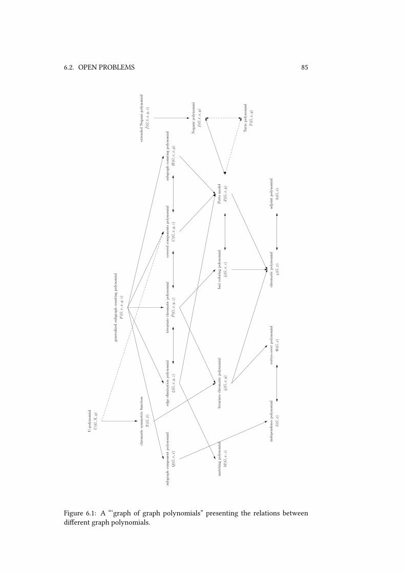
6.2. OPEN PROBLEMS 85
generalized
subgrap
hcountingpolynom
ial
F(G
,v,x,y,z)
U-polynom
ial
U(G
,X,y)
chromatic
symmetricfunction
X(G
,x)
extended
Negam
ipolynom
ial
f(G
,t,x,y,z)
edge
elim
inationpolynom
ial
ξ(G,x,y,z)
coveredcompon
ents
polynom
ial
C(G
,x,y,z)
subgrap
hcountingpolynom
ial
H(G
,v,x,y)
trivariate
chromatic
polynom
ial
P(G
,x,y,z)
subgrap
hcompon
entpolynom
ial
Q(G
,v,x)
bad
coloringpolynom
ial
χ(G
,x,z)
bivariate
chromatic
polynom
ial
χ(G
,x,y)
Potts
model
Z(G
,x,y)
Negam
ipolynom
ial
f(G
,t,x,y)
Tuttepolynom
ial
T(G
,x,y)
adjointpolynom
ial
h(G
,x)
chromatic
polynom
ial
χ(G
,x)
matchingpolynom
ial
M(G
,x,z)
indep
endence
polynom
ial
I(G
,x)
vertex-cover
polynom
ial
Ψ(G
,x)
Figure 6.1: A “‘graph of graph polynomials” presenting the relations betweendiUerent graph polynomials.

86 CHAPTER 6. CONCLUSION
The generalized subgraph counting polynomial generalizes the trivariatechromatic polynomial. Can the generalized subgraph counting polynomial bedeVned in terms of colorings which makes this relation obvious?
Question 5. Is there a coloring expansion of the generalized subgraph countingpolynomial?
There are some other graph polynomials generalizing the same graph polyno-mials as the generalized subgraph counting polynomial. It seems that the relationbetween these graph polynomials is not yet considered.
Question 6. Are the generalized subgraph counting polynomial, the extendedNegami polynomial, and the homomorphism polynomial related to each other (forgraphs / forests)?
Question 7. Is the generalized subgraph counting polynomial a “most generalgraph polynomial” with respect to the recurrence relation it satisVes?
If we restrict the recurrence relations to those with δ = 0, is then the edgeelimination polynomial also most general or are by the independence of the fac-tors for a link and a loop other graph polynomials possible?
Question 8. Is there a most general graph polynomial satisfying Theorem 5.16 inthe case δ = 0?
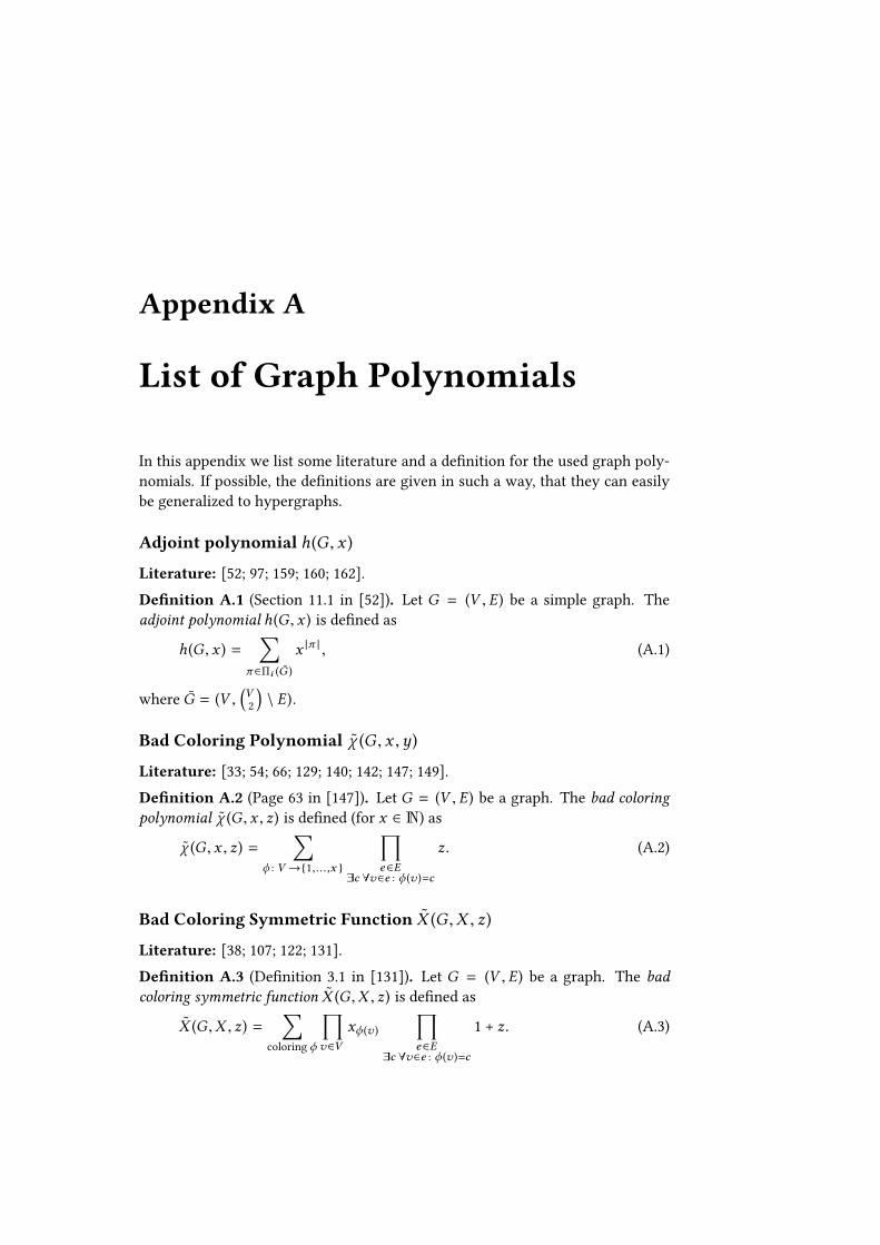
Appendix A
List of Graph Polynomials
In this appendix we list some literature and a deVnition for the used graph poly-nomials. If possible, the deVnitions are given in such a way, that they can easilybe generalized to hypergraphs.
Adjoint polynomial h(G , x )
Literature: [52; 97; 159; 160; 162].
DeVnition A.1 (Section 11.1 in [52]). Let G = (V , E) be a simple graph. Theadjoint polynomial h(G , x ) is deVned as
h(G , x ) =∑
π∈Πi (G )
x |π | , (A.1)
where G = (V ,(V2
)\ E).
Bad Coloring Polynomial χ (G , x ,y)
Literature: [33; 54; 66; 129; 140; 142; 147; 149].
DeVnition A.2 (Page 63 in [147]). Let G = (V , E) be a graph. The bad coloringpolynomial χ (G , x , z) is deVned (for x ∈ N) as
χ (G , x , z) =∑
ϕ : V →{1,...,x }
∏e∈E
∃c ∀v∈e : ϕ (v )=c
z. (A.2)
Bad Coloring Symmetric Function X (G ,X , z)
Literature: [38; 107; 122; 131].
DeVnition A.3 (DeVnition 3.1 in [131]). Let G = (V , E) be a graph. The badcoloring symmetric function X (G ,X , z) is deVned as
X (G ,X , z) =∑
coloring ϕ
∏v∈V
xϕ (v )
∏e∈E
∃c ∀v∈e : ϕ (v )=c
1 + z. (A.3)

88 APPENDIX A. LIST OF GRAPH POLYNOMIALS
Bivariate Chromatic Polynomial P (G , x ,y)
Literature: [4; 5; 49; 50; 73; 77; 78].
DeVnition A.4 (Section 1 in [50]). Let G = (V , E) be a graph. The bivariatechromatic polynomial P (G , x ,y) is deVned as
P (G , x ,y) =∑
ϕ : V →{1,...,x }
∏e∈E
∃c≤y ∀v∈e : ϕ (v )=c
0. (A.4)
Characteristic Polynomial ϕ (G , x )
Literatur[44; 67; 80; 117; 119; 136]
DeVnition A.5 (Section 0.1 in [44]). Let G = (V , E) be a graph with adjacencymatrix A(G ). The characteristic polynomial ϕ (G , x ) is deVned as
ϕ (G , x ) = det(xI − A(G )) , (A.5)
where I is the identity matrix of format |V | × |V |.
Chromatic Polynomial χ (G , x )
Literature: [8; 13; 14; 16; 17; 18; 19; 20; 23; 37; 52; 103; 112; 114; 115; 128; 141;151; 152; 153; 161].
DeVnition A.6 ([18], Section 2 in [151]). Let G = (V , E) be a graph. The chro-matic polynomial χ (G , x ) is deVned (for x ∈ N) as
χ (G , x ) =∑
ϕ : V →{1,...,x }
∏e∈E
∃c ∀v∈e : ϕ (v )=c
0. (A.6)
Chromatic Symmetric Function X (G ,X )
Literature: [38; 101; 130; 131].
DeVnition A.7 (DeVnition 2.1 in [130]). Let G = (V , E) be a graph. The chro-matic symmetric function X (G ,X ) is deVned as
X (G ,X ) =∑
proper coloring ϕ
∏v∈V
xϕ (v ) . (A.7)
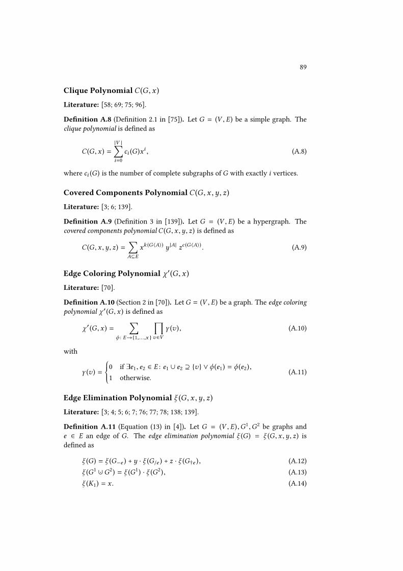
89
Clique Polynomial C (G , x )
Literature: [58; 69; 75; 96].
DeVnition A.8 (DeVnition 2.1 in [75]). Let G = (V , E) be a simple graph. Theclique polynomial is deVned as
C (G , x ) =|V |∑i=0
ci (G )xi , (A.8)
where ci (G ) is the number of complete subgraphs of G with exactly i vertices.
Covered Components Polynomial C (G , x ,y , z)
Literature: [3; 6; 139].
DeVnition A.9 (DeVnition 3 in [139]). Let G = (V , E) be a hypergraph. Thecovered components polynomial C (G , x ,y , z) is deVned as
C (G , x ,y , z) =∑A⊆E
xk (G 〈A〉) y |A| zc (G 〈A〉) . (A.9)
Edge Coloring Polynomial χ ′(G , x )
Literature: [70].
DeVnition A.10 (Section 2 in [70]). LetG = (V , E) be a graph. The edge coloringpolynomial χ ′(G , x ) is deVned as
χ ′(G , x ) =∑
ϕ : E→{1,...,x }
∏v∈V
γ (v ), (A.10)
with
γ (v ) =
0 if ∃e1 , e2 ∈ E : e1 ∪ e2 ⊇ {v} ∨ ϕ (e1) = ϕ (e2),
1 otherwise.(A.11)
Edge Elimination Polynomial ξ (G , x ,y , z)
Literature: [3; 4; 5; 6; 7; 76; 77; 78; 138; 139].
DeVnition A.11 (Equation (13) in [4]). Let G = (V , E),G1 ,G2 be graphs ande ∈ E an edge of G. The edge elimination polynomial ξ (G ) = ξ (G , x ,y , z) isdeVned as
ξ (G ) = ξ (G−e ) + y · ξ (G/e ) + z · ξ (G†e ), (A.12)
ξ (G1 ∪· G2) = ξ (G1) · ξ (G2), (A.13)
ξ (K1) = x . (A.14)
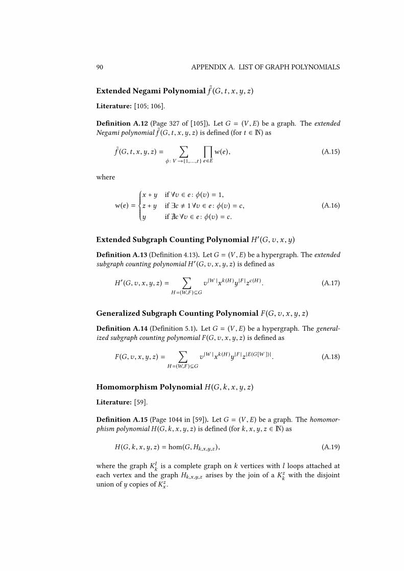
90 APPENDIX A. LIST OF GRAPH POLYNOMIALS
Extended Negami Polynomial f (G , t , x ,y , z)
Literature: [105; 106].
DeVnition A.12 (Page 327 of [105]). Let G = (V , E) be a graph. The extendedNegami polynomial f (G , t , x ,y , z) is deVned (for t ∈ N) as
f (G , t , x ,y , z) =∑
ϕ : V →{1,...,t }
∏e∈E
w (e ), (A.15)
where
w (e ) =
x + y if ∀v ∈ e : ϕ (v ) = 1,
z + y if ∃c , 1∀v ∈ e : ϕ (v ) = c ,y if @c ∀v ∈ e : ϕ (v ) = c .
(A.16)
Extended Subgraph Counting Polynomial H ′(G ,v , x ,y)
DeVnition A.13 (DeVnition 4.13). LetG = (V , E) be a hypergraph. The extendedsubgraph counting polynomial H ′(G ,v , x ,y , z) is deVned as
H ′(G ,v , x ,y , z) =∑
H =(W,F )⊆G
v |W |xk (H )y |F |zc (H ) . (A.17)
Generalized Subgraph Counting Polynomial F (G ,v , x ,y , z)
DeVnition A.14 (DeVnition 5.1). Let G = (V , E) be a hypergraph. The general-ized subgraph counting polynomial F (G ,v , x ,y , z) is deVned as
F (G ,v , x ,y , z) =∑
H =(W,F )⊆G
v |W |xk (H )y |F |z |E (G [W ]) | . (A.18)
Homomorphism Polynomial H (G , k , x ,y , z)
Literature: [59].
DeVnition A.15 (Page 1044 in [59]). Let G = (V , E) be a graph. The homomor-phism polynomial H (G , k , x ,y , z) is deVned (for k , x ,y , z ∈ N) as
H (G , k , x ,y , z) = hom(G ,Hk,x,y,z ), (A.19)
where the graph Klk is a complete graph on k vertices with l loops attached at
each vertex and the graph Hk,x,y,z arises by the join of a Kzk with the disjoint
union of y copies of Kzx .
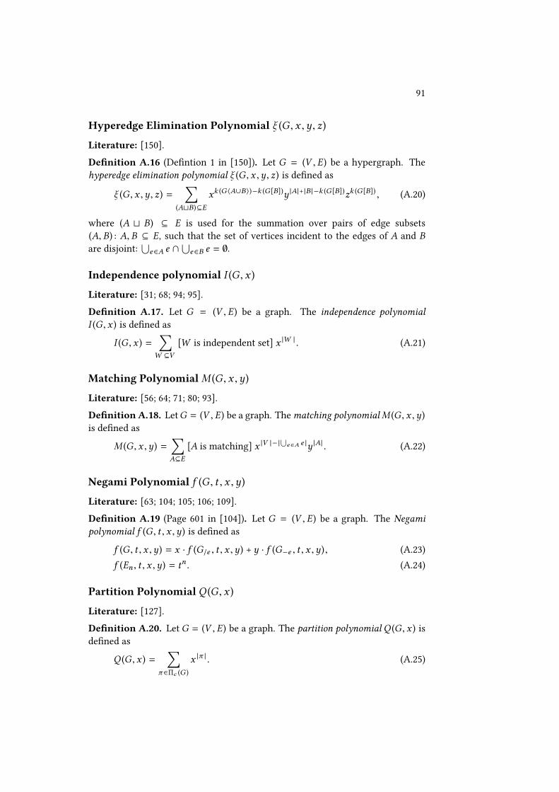
91
Hyperedge Elimination Polynomial ξ (G , x ,y , z)
Literature: [150].
DeVnition A.16 (DeVntion 1 in [150]). Let G = (V , E) be a hypergraph. Thehyperedge elimination polynomial ξ (G , x ,y , z) is deVned as
ξ (G , x ,y , z) =∑
(AtB)⊆E
xk (G 〈A∪B〉)−k (G [B])y |A|+|B |−k (G [B])zk (G [B]) , (A.20)
where (A t B) ⊆ E is used for the summation over pairs of edge subsets(A, B) : A, B ⊆ E, such that the set of vertices incident to the edges of A and Bare disjoint:
⋃e∈A e ∩
⋃e∈B e = ∅.
Independence polynomial I (G , x )
Literature: [31; 68; 94; 95].
DeVnition A.17. Let G = (V , E) be a graph. The independence polynomialI (G , x ) is deVned as
I (G , x ) =∑
W ⊆V
[W is independent set] x |W | . (A.21)
Matching PolynomialM (G , x ,y)
Literature: [56; 64; 71; 80; 93].
DeVnition A.18. LetG = (V , E) be a graph. The matching polynomial M (G , x ,y)is deVned as
M (G , x ,y) =∑A⊆E
[A is matching] x |V |− |⋃e∈A e |y |A| . (A.22)
Negami Polynomial f (G , t , x ,y)
Literature: [63; 104; 105; 106; 109].
DeVnition A.19 (Page 601 in [104]). Let G = (V , E) be a graph. The Negamipolynomial f (G , t , x ,y) is deVned as
f (G , t , x ,y) = x · f (G/e , t , x ,y) + y · f (G−e , t , x ,y), (A.23)
f (En , t , x ,y) = tn . (A.24)
Partition Polynomial Q (G , x )
Literature: [127].
DeVnition A.20. Let G = (V , E) be a graph. The partition polynomial Q (G , x ) isdeVned as
Q (G , x ) =∑
π∈Πc (G )
x |π | . (A.25)
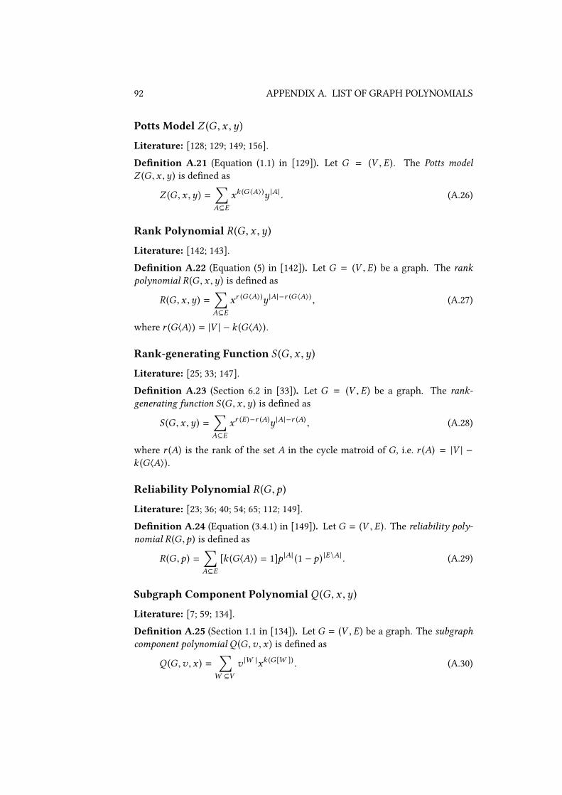
92 APPENDIX A. LIST OF GRAPH POLYNOMIALS
Potts Model Z (G , x ,y)
Literature: [128; 129; 149; 156].
DeVnition A.21 (Equation (1.1) in [129]). Let G = (V , E). The Potts modelZ (G , x ,y) is deVned as
Z (G , x ,y) =∑A⊆E
xk (G 〈A〉)y |A| . (A.26)
Rank Polynomial R (G , x ,y)
Literature: [142; 143].
DeVnition A.22 (Equation (5) in [142]). Let G = (V , E) be a graph. The rankpolynomial R (G , x ,y) is deVned as
R (G , x ,y) =∑A⊆E
xr (G 〈A〉)y |A|−r (G 〈A〉) , (A.27)
where r (G〈A〉) = |V | − k (G〈A〉).
Rank-generating Function S (G , x ,y)
Literature: [25; 33; 147].
DeVnition A.23 (Section 6.2 in [33]). Let G = (V , E) be a graph. The rank-generating function S (G , x ,y) is deVned as
S (G , x ,y) =∑A⊆E
xr (E )−r (A)y |A|−r (A) , (A.28)
where r (A) is the rank of the set A in the cycle matroid of G, i.e. r (A) = |V | −k (G〈A〉).
Reliability Polynomial R (G ,p)
Literature: [23; 36; 40; 54; 65; 112; 149].
DeVnition A.24 (Equation (3.4.1) in [149]). Let G = (V , E). The reliability poly-nomial R (G ,p) is deVned as
R (G ,p) =∑A⊆E
[k (G〈A〉) = 1]p |A| (1 − p) |E\A| . (A.29)
Subgraph Component Polynomial Q (G , x ,y)
Literature: [7; 59; 134].
DeVnition A.25 (Section 1.1 in [134]). Let G = (V , E) be a graph. The subgraphcomponent polynomial Q (G ,v , x ) is deVned as
Q (G ,v , x ) =∑
W ⊆V
v |W |xk (G [W ]) . (A.30)
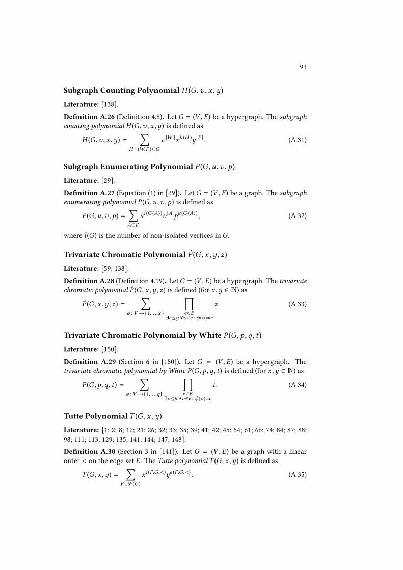
93
Subgraph Counting Polynomial H (G ,v , x ,y)
Literature: [138].
DeVnition A.26 (DeVnition 4.8). Let G = (V , E) be a hypergraph. The subgraphcounting polynomial H (G ,v , x ,y) is deVned as
H (G ,v , x ,y) =∑
H =(W,F )⊆G
v |W |xk (H )y |F | . (A.31)
Subgraph Enumerating Polynomial P (G ,u ,v ,p)
Literature: [29].
DeVnition A.27 (Equation (1) in [29]). Let G = (V , E) be a graph. The subgraphenumerating polynomial P (G ,u ,v ,p) is deVned as
P (G ,u ,v ,p) =∑A⊆E
ui (G 〈A〉)v |A|pk (G 〈A〉) , (A.32)
where i (G ) is the number of non-isolated vertices in G.
Trivariate Chromatic Polynomial P (G , x ,y , z)
Literature: [59; 138].
DeVnition A.28 (DeVnition 4.19). LetG = (V , E) be a hypergraph. The trivariatechromatic polynomial P (G , x ,y , z) is deVned (for x ,y ∈ N) as
P (G , x ,y , z) =∑
ϕ : V →{1,...,x }
∏e∈E
∃c≤y ∀v∈e : ϕ (v )=c
z. (A.33)
Trivariate Chromatic Polynomial by White P (G ,p ,q, t )
Literature: [150].
DeVnition A.29 (Section 6 in [150]). Let G = (V , E) be a hypergraph. Thetrivariate chromatic polynomial by White P (G ,p ,q, t ) is deVned (for x ,y ∈ N) as
P (G ,p ,q, t ) =∑
ϕ : V →{1,...,q}
∏e∈E
∃c≤p ∀v∈e : ϕ (v )=c
t . (A.34)
Tutte Polynomial T (G , x ,y)
Literature: [1; 2; 8; 12; 21; 26; 32; 33; 35; 39; 41; 42; 45; 54; 61; 66; 74; 84; 87; 88;98; 111; 113; 129; 135; 141; 144; 147; 148].
DeVnition A.30 (Section 3 in [141]). Let G = (V , E) be a graph with a linearorder < on the edge set E. The Tutte polynomial T (G , x ,y) is deVned as
T (G , x ,y) =∑
F ∈F (G )
xi (F,G,<)ye (F,G,<) . (A.35)
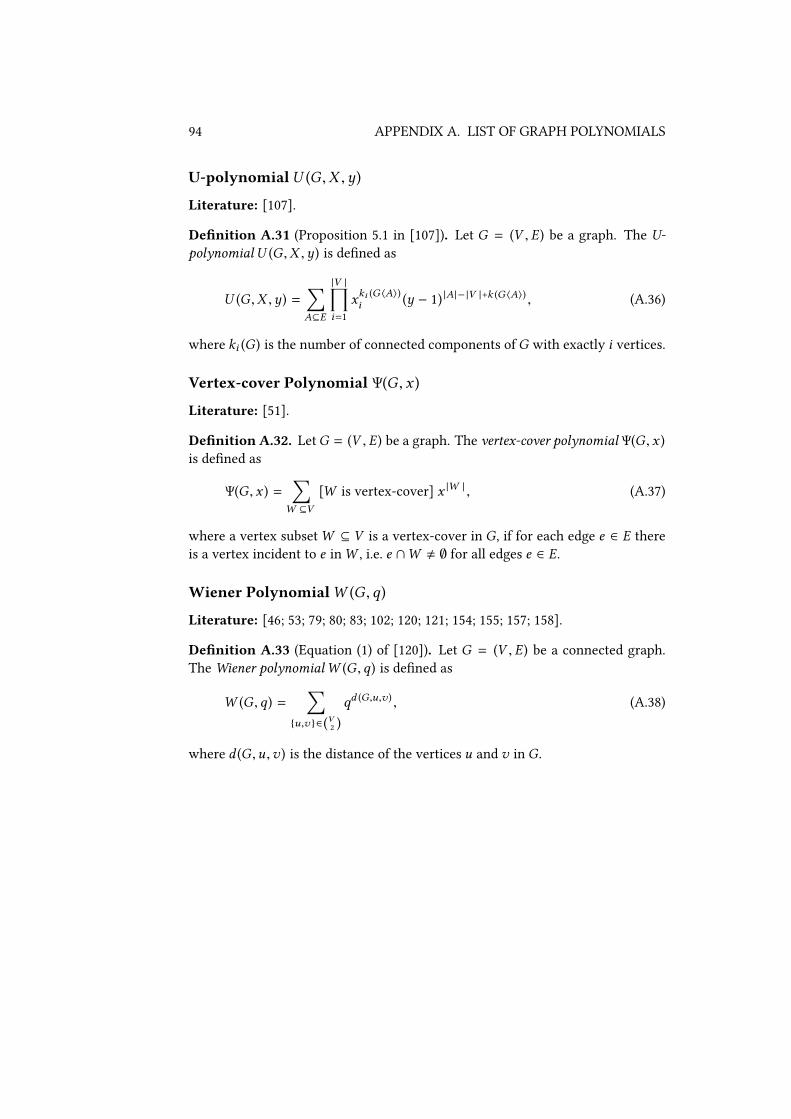
94 APPENDIX A. LIST OF GRAPH POLYNOMIALS
U-polynomialU (G ,X ,y)
Literature: [107].
DeVnition A.31 (Proposition 5.1 in [107]). Let G = (V , E) be a graph. The U-polynomial U (G ,X ,y) is deVned as
U (G ,X ,y) =∑A⊆E
|V |∏i=1
xki (G 〈A〉)i (y − 1) |A|− |V |+k (G 〈A〉) , (A.36)
where ki (G ) is the number of connected components ofG with exactly i vertices.
Vertex-cover Polynomial Ψ(G , x )
Literature: [51].
DeVnition A.32. LetG = (V , E) be a graph. The vertex-cover polynomial Ψ(G , x )is deVned as
Ψ(G , x ) =∑
W ⊆V
[W is vertex-cover] x |W | , (A.37)
where a vertex subsetW ⊆ V is a vertex-cover in G, if for each edge e ∈ E thereis a vertex incident to e inW , i.e. e ∩W , ∅ for all edges e ∈ E.
Wiener PolynomialW (G ,q)
Literature: [46; 53; 79; 80; 83; 102; 120; 121; 154; 155; 157; 158].
DeVnition A.33 (Equation (1) of [120]). Let G = (V , E) be a connected graph.The Wiener polynomialW (G ,q) is deVned as
W (G ,q) =∑
{u,v }∈(V2 )
qd (G,u,v ) , (A.38)
where d (G ,u ,v ) is the distance of the vertices u and v in G.
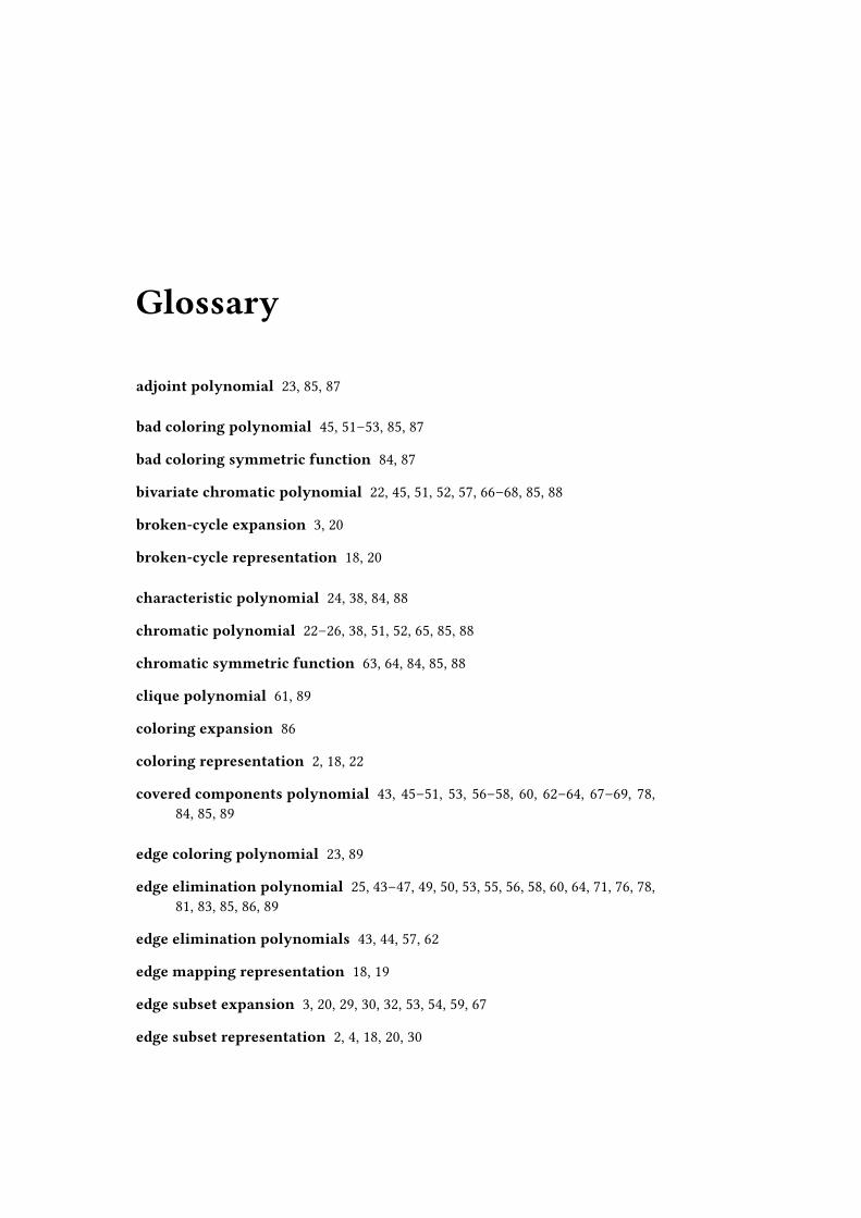
Glossary
adjoint polynomial 23, 85, 87
bad coloring polynomial 45, 51–53, 85, 87
bad coloring symmetric function 84, 87
bivariate chromatic polynomial 22, 45, 51, 52, 57, 66–68, 85, 88
broken-cycle expansion 3, 20
broken-cycle representation 18, 20
characteristic polynomial 24, 38, 84, 88
chromatic polynomial 22–26, 38, 51, 52, 65, 85, 88
chromatic symmetric function 63, 64, 84, 85, 88
clique polynomial 61, 89
coloring expansion 86
coloring representation 2, 18, 22
covered components polynomial 43, 45–51, 53, 56–58, 60, 62–64, 67–69, 78,84, 85, 89
edge coloring polynomial 23, 89
edge elimination polynomial 25, 43–47, 49, 50, 53, 55, 56, 58, 60, 64, 71, 76, 78,81, 83, 85, 86, 89
edge elimination polynomials 43, 44, 57, 62
edge mapping representation 18, 19
edge subset expansion 3, 20, 29, 30, 32, 53, 54, 59, 67
edge subset representation 2, 4, 18, 20, 30

96 GLOSSARY
extended Negami polynomial 66, 67, 84–86, 90
extended subgraph counting polynomial 43, 49–51, 58, 77, 78, 90
generalized subgraph counting polynomial 71–78, 81, 85, 86, 90
generating function representation 18, 19
homomorphism polynomial 24, 76, 86, 90
homomorphism representation 18, 19
hyperedge elimination polynomial 43, 55, 91
independence polynomial 61, 85, 91
matching polynomial 45, 85, 91
matrix representation 18, 19
matroid representation 18, 19
Negami polynomial 66, 84, 85, 91
partition polynomial 22, 91
partition representation 18
Potts model 25, 41, 45, 47, 61, 62, 65, 66, 76, 77, 81, 84, 85, 92
rank polynomial 60, 61, 92
rank-generating function 25, 92
recurrence relation representation 18, 19
reliability domination expansion 20
reliability domination representation 18, 20
reliability polynomial 92
spanning forest expansion 21, 30, 33, 34
spanning forest representation 4, 18, 20, 30
spanning tree representation 20
spin model 18, 21

GLOSSARY 97
spin model expansion 22
state model 21
subgraph component polynomial 64–66, 71, 73–77, 85, 92
subgraph counting polynomial 43, 47–51, 54, 59–62, 64–66, 71, 73–75, 77, 78,85, 93
subgraph enumerating polynomial 43, 56, 59, 93
subgraph expansion 19
subgraph representation 18
trivariate chromatic polynomial 43, 51–55, 57–59, 66–68, 84–86, 93
trivariate chromatic polynomial (White) 43, 57, 93
Tutte polynomial 41, 45, 66, 84, 85, 93
U-polynomial 62–64, 84, 85, 94
value representation 18, 19
vertex mapping representation 18
vertex model 18, 19
vertex subset expansion 21, 47, 57, 61, 65, 76, 77
vertex subset representation 18, 21
vertex-cover polynomial 45, 85, 94
weighted graph polynomial 22, 62
Wiener polynomial 68, 69, 84, 94

98 GLOSSARY

Bibliography
[1] Martin Aigner. A Course in Enumeration. Vol. 238. Graduate Texts inMathematics. Berlin: Springer, 2007. doi: 10.1007/978-3-540-39035-0.
[2] Artur Andrzejak. “An algorithm for the Tutte polynomials of graphs ofbounded treewidth”. In: Discrete Mathematics 190.1-3 (1998), pp. 39–54.doi: 10.1016/S0012-365X(98)00113-7.
[3] Ilia Averbouch. “Completeness and Universality Properties of Graph In-variants and Graph Polynomials”. PhD thesis. Israel Institute of Technol-ogy, Nov. 2010. url: http://cs.technion.ac.il/~ailia/thesis/Work/thesis.pdf.
[4] Ilia Averbouch, Benny Godlin, and Johann A. Makowsky. “A most generaledge elimination polynomial”. In: Graph-Theoretic Concepts in ComputerScience. Vol. 5344. Lecture Notes in Computer Science. Springer Berlin /Heidelberg, 2008, pp. 31–42. doi: 10.1007/978-3-540-92248-3_4.
[5] Ilia Averbouch, Benny Godlin, and Johann A. Makowsky. “An extensionof the bivariante chromatic polynomial”. In: European Journal of Combi-natorics 31.1 (2010), pp. 1–17. doi: 10.1016/j.ejc.2009.05.006.
[6] Ilia Averbouch, Tomer Kotek, Johann A. Makowsky, and E. Ravve. “TheUniversal Edge Elimination Polynomial and the Dichromatic Polynomial”.In: Electronic Notes in Discrete Mathematics 38.0 (2011). The Sixth Euro-pean Conference on Combinatorics, Graph Theory and Applications, Eu-roComb 2011, pp. 77–82. doi: 10.1016/j.endm.2011.09.013.
[7] Ilia Averbouch, Johann A. Makowsky, and Peter Tittmann. “A graph poly-nomial arising from community structure (extended abstract)”. In: Graph-Theoretic Concepts in Computer Science. Ed. by C. Paul and M. Habib.Vol. 5911. Lecture Notes in Computer Science. 2010, pp. 33–43. doi: 10.1007/978-3-642-11409-0_3.
[8] Ruth A. Bari. “Chromatic Polynomials and the Internal and External Ac-tivities of Tutte”. In: Graph Theory and Related Topics. Ed. by J. A. Bondyand U. S. R. Murty. Proceedings of the conference held in honour of Pro-fessor W. T. Tutte on the occasion of his sixtieth birthday, University ofWaterloo, July 5-9, 1977. London: Academic Press, 1979, pp. 41–52.
100 BIBLIOGRAPHY
[9] Ruth A. Bari. “Homomorphism polynomials of graphs”. In: Journal ofCombinatorics, Information & System Sciences 7.1 (1982), pp. 56–64.
[10] Claude Berge. Graphs and hypergraphs. North-Holland, 1973. GoogleBooks: Wy2mhanRnk4C.
[11] Claude Berge. Hypergraphs. Vol. 45. North-Holland Mathematical Li-brary. North-Holland, 1989. url: http://www.sciencedirect.com/science/bookseries/09246509/45.
[12] Olivier Bernardi. “A Characterization of the Tutte Polynomial via Com-binatorial Embeddings”. In: Annals of Combinatorics 12.2 (2008), pp. 139–153. doi: 10.1007/s00026-008-0343-4.
[13] Pascal Berthomé, Sylvain Lebresne, and Kim Nguyên. “Computationof Chromatic Polynomials Using Triangulations and Clique Trees”. In:Graph-Theoretic Concepts in Computer Science. Ed. by Dieter Kratsch.Vol. 3787. Lecture Notes in Computer Science. Springer Berlin / Heidel-berg, 2005, pp. 362–373. doi: 10.1007/11604686_32.
[14] Norman L. Biggs. “Expansions of the chromatic polynomial”. In: DiscreteMathematics 6.2 (1973), pp. 105–113. doi: 10 . 1016 / 0012 - 365X(73 )90040-X.
[15] Norman L. Biggs. Algebraic graph theory. Vol. 2. Cambridge: CambridgeUniversity Press, 1993.
[16] Norman L. Biggs. “A matrix method for chromatic polynomials - II”. In:LSE-CDAM 2000-04. CDAM Research Report Series. 2000.
[17] Norman L. Biggs. “A Matrix Method for Chromatic Polynomials”. In: Jour-nal of Combinatorial Theory, Series B 82.1 (2001), pp. 19–29. doi: 10.1006/jctb.2000.2017.
[18] George D. BirkhoU. “A Determinant Formula for the Number of Ways ofColoring a Map”. In: The Annals of Mathematics 14.1 (1912), pp. 42–46.JSTOR: 1967597.
[19] George D. BirkhoU. “On the polynomial expressions for the number ofways of coloring a map”. In: Annali Pisa 3.1 (1934), pp. 85–103. url: http://www.numdam.org/item?id=ASNSP_1934_2_3_1_85_0.
[20] George D. BirkhoU and D. C. Lewis. “Chromatic polynomials”. In: Trans-actions of the American Mathematical Society 60 (1946), pp. 355–451. doi:10.1090/S0002-9947-1946-0018401-4.
[21] Andreas Björklund, Thore Husfeldt, Petteri Kaski, and Mikko Koivisto.Computing the Tutte polynomial in vertex-exponential time. Apr. 2008.arXiv: 0711.2585 [cs.DS].
[22] Anders Björner. “Homology and Shellability of Matroids and GeometricLattices”. In: Matroid Applications. Ed. by Neil White. Cambridge Univer-sity Press, 1992, pp. 226–283. doi: 10.1017/CBO9780511662041.
BIBLIOGRAPHY 101
[23] F. T. Boesch, A. Satyanarayana, and C. L. SuUel. “Some Alternate Char-acterizations of Reliability Domination”. In: Probability in the Engineer-ing and Informational Sciences 4 (1990), pp. 257–276. doi: 10 . 1017 /S0269964800001571.
[24] F. T. Boesch, A. Satyanarayana, and C. L. SuUel. “A survey of some net-work reliability analysis and synthesis results”. In: Networks 54 (2009),pp. 99–107. doi: 10.1002/net.20300.
[25] Béla Bollobás. Modern Graph Theory. Vol. 184. Graduate Texts in Mathe-matics. Springer New York, 1998.
[26] Béla Bollobás, Luke Pebody, and Oliver Riordan. “Contraction-deletioninvariants for graphs”. In: Journal of Combinatorial Theory, Series B 80.2(2000), pp. 320–345. doi: 10.1006/jctb.2000.1988.
[27] J. A. Bondy and U. S. R. Murty, eds. Graph theory and related topics. Pro-ceedings of the conference held in honour of Professor W. T. Tutte on theoccasion of his sixtieth birthday, University of Waterloo, July 5-9, 1977.Academic Press, 1979.
[28] J. A. Bondy and U. S. R. Murty. Graph Theory. Vol. 244. Graduate Texts inMathematics. Berlin: Springer, 2008. doi: 10.1007/978-1-84628-970-5.
[29] Luigi Borzacchini and Carmelo Pulito. “On subgraph enumerating poly-nomials and Tutte polynomials”. In: Bollettino U. M. I. 6.1-B (1982),pp. 589–597.
[30] Boštjan Brešar, Wilfried Imrich, and Sandi Klavžar. “Reconstructingsubgraph-counting graph polynomials of increasing families of graphs”.In: Discrete Mathematics 297.1-3 (2005), pp. 159–166. doi: 10.1016/j.disc.2005.02.019.
[31] Jason Brown and Richard Hoshino. On Circulant Graphs Uniquely Charac-terized by their Independence Polynomials. 2011. url: http://research.nii.ac.jp/~rhoshino/papers/ipunique.pdf.
[32] Thomas H. Brylawski. “Intersection Theory for Graphs”. In: Journal ofCombinatorial Theory, Series B 30.2 (1981), pp. 233–246. doi: 10.1016/0095-8956(81)90068-X.
[33] Thomas H. Brylawski and James G. Oxley. “The Tutte Polynomial and ItsApplications”. In: Matroid Applications. Ed. by Neil White. Vol. 40. Ency-clopedia of mathematics and its applications. Cambridge University Press,1992. Chap. 6, pp. 123–225.
[34] Jesper Makholm Byskov. “Enumerating maximal independent sets withapplications to graph colouring”. In: Operations Research Letters 32.6(2004), pp. 547–556. doi: 10.1016/j.orl.2004.03.002.
102 BIBLIOGRAPHY
[35] Hungyung Chang, Jun Ma, and Yeong-Nan Yeh. “Tutte polynomials andG-parking functions”. In: Advances in Applied Mathematics 44.3 (2010),pp. 231–242. doi: 10.1016/j.aam.2009.07.001.
[36] M. Chari and Charles J. Colbourn. “Reliability Polynomials: A Survey”.In: Journal of Combinatorics, Information and System Scienes 22 (1997),pp. 177–193.
[37] G. L. Chia. “A bibliography on chromatic polynomials”. In: Discrete Math-ematics 172.1-3 (1997), pp. 175–191. doi: 10.1016/S0012- 365X(97)90031-5.
[38] Timothy Yi-Chung Chow. “Symmetric function generalizations of graphpolynomials”. PhD thesis. Massachusetts Institute of Technology, Mar.1995. arXiv: math/0103229 [math.COel].
[39] Laura E. Chávez-Lomelí, Criel Merino, Steven D. Noble, and MarcelinoRamírez-Ibáñez. “Some inequalities for the Tutte polynomial”. In: Euro-pean Journal of Combinatorics 32.3 (2011), pp. 422–433. doi: 10.1016/j.ejc.2010.11.005.
[40] Charles J. Colbourn. The Combinatorics of Network Reliability. New York,NY, USA: Oxford University Press, 1987.
[41] Charles J. Colbourn and William R. Pulleyblank. “Matroid Steiner prob-lems, the Tutte polynomial and network reliability”. In: Journal of Com-binatorial Theory, Series B 47.1 (1989), pp. 20–31. doi: 10.1016/0095-8956(89)90062-2.
[42] Henry H. Crapo. “The Tutte polynomial”. In: Aequationes Mathematicae3.3 (1969), pp. 211–229. doi: 10.1007/BF01817442.
[43] Péter Csikvári. “Graph Polynomials and Graph Transformations in Alge-braic Graph Theory”. PhD thesis. Eötvös Loránd University, 2011. url:http://teo.elte.hu/minosites/ertekezes2011/csikvari_p.pdf.
[44] Dragos M. Cvetković, Michael Doob, and H. Sachs. Spectra of Graphs. 3rd.Johann Ambrosius Barth, 1995.
[45] Jeremy Dawson. “A construction for a family of sets and its applicationto matroids”. In: Combinatorial Mathematics VIII. Vol. 884. Lecture Notesin Mathematics. Springer Berlin / Heidelberg, 1981, pp. 136–147. doi: 10.1007/BFb0091815.
[46] Matthias Dehmer and Aleksandar Ilić. “Location of Zeros of Wiener andDistance Polynomials”. In: PLoS ONE 7.3 (Mar. 2012), e28328. doi: 10.1371/journal.pone.0028328.
[47] Reinhard Diestel. Graph Theory. 3rd. Vol. 173. Graduate Texts in Math-ematics. Springer Berlin / Heidelberg / New York, 2005. url: http://diestel-graph-theory.com.

BIBLIOGRAPHY 103
[48] Klaus Dohmen. “An Inductive Proof of Whitney’s Broken Circuit Theo-rem”. In: Discussiones Mathematicae Graph Theory 31 (2011), pp. 509–515.
[49] Klaus Dohmen. Closed-form expansions for the bivariate chromatic polyno-mial of paths and cycles. Jan. 2012. arXiv: 1201.3886 [math.CO].
[50] Klaus Dohmen, André Pönitz, and Peter Tittmann. “A new two-variablegeneralization of the chromatic polynomial”. In: Discrete Mathematics andTheoretical Computer Science 6 (2003), pp. 69–90. url: http://www.emis.de/journals/DMTCS/volumes/abstracts/dm060106.abs.html.
[51] F. M. Dong, M. D. Hendy, K. L. Teo, and C. H. C. Little. “The vertex-coverpolynomial of a graph”. In: Discrete Mathematics 250.1 - 3 (2002), pp. 71–78. doi: 10.1016/S0012-365X(01)00272-2.
[52] F. M. Dong, K. M. Koh, and K. L. Teo. Chromatic polynomials and chro-maticity of graphs. World ScientiVc Publishing, 2005.
[53] Mehdi Eliasi and Bijan Taeri. “Extension of the Wiener index and Wienerpolynomial”. In: Applied Mathematics Letters 21 (2008), pp. 916–921. doi:10.1016/j.aml.2007.10.001.
[54] Joanna A. Ellis-Monaghan and Criel Merino. “Graph polynomials andtheir applications I: The Tutte polynomial”. In: Structural Analysis of Com-plex Networks. Ed. by Matthias Dehmer. Birkhäuser Boston, 2011. Chap. 9,pp. 219–255. doi: 10.1007/978-0-8176-4789-6_9.
[55] Joanna A. Ellis-Monaghan and Criel Merino. “Graph polynomials andtheir applications II: Interrelations and interpretations”. In: StructuralAnalysis of Complex Networks. Ed. by Matthias Dehmer. BirkhäuserBoston, 2011. Chap. 10, pp. 257–292. doi: 10.1007/978-0-8176-4789-6_10.
[56] Edward J. Farrell. “An Introduction to Matching Polynomials”. In: Journalof Combinatorial Theory, Series B 27.1 (1979), pp. 75–86. doi: 10.1016/0095-8956(79)90070-4.
[57] Edward J. Farrell and S. A. Wahid. “On the reconstraction of the matchingpolynomial and the reconstruction conjecture”. In: International Journalof Mathematics and Mathematical Sciences 10.1 (1987), pp. 155–162. doi:10.1155/S016117128700019X.
[58] David C. Fisher and Anita E. Solow. “Dependence polynomials”. In:Discrete Mathematics 82.3 (1990), pp. 251–258. doi: 10 . 1016 / 0012 -365X(90)90202-S.
[59] Delia Garijo, Andrew Goodall, and Jaroslav Nešetřil. “Distinguishinggraphs by their left and right homomorphism proVles”. In: European Jour-nal of Combinatorics 32.7 (2011), pp. 1025–1053. doi: 10.1016/j.ejc.2011.03.012.
104 BIBLIOGRAPHY
[60] Delia Garijo, Jaroslav Nešetřil, and M. Pastora Revuelta. “Homomor-phisms and polynomial invariants of graphs”. In: European Journal ofCombinatorics 30.7 (2009), pp. 1659–1675. doi: 10.1016/j.ejc.2009.03.016.
[61] Ira M. Gessel and Bruce E. Sagan. “The Tutte polynomial of a graph,depth-Vrst search, and simplicial complex partitions”. In: The ElectronicJournal of Combinatorics 3.2 (1996). The Foata Festschrift, #R9. url: http://www.combinatorics.org/Volume_3/volume3_2.html#R9.
[62] Richard Alan Gillman. “Homomorphism and sigma polynomials”. In: In-ternational Journal of Mathematics and Mathematical Sciences 18.4 (1995),pp. 653–658. doi: 10.1155/S0161171295000834.
[63] Richard Alan Gillman. “Negami’s polynomial as a contraction polyno-mial”. In: Proceedings of the seventh quadrennial international conferenceon the theory and applications of graphs. Ed. by Y. Alavi and A. Schwenk.Vol. 1. Graph theory, combinatorics, algorithms and applications. NewYork, NY: Wiley, 1995.
[64] Chris D. Godsil and Ivan Gutman. “On the theory of the matching polyno-mial”. In: Journal of Graph Theory 5.2 (1981), pp. 137–144. doi: 10.1002/jgt.3190050203.
[65] Chris D. Godsil and Gordon Royle. Algebraic graph theory. Vol. 207. Grad-uate Texts in Mathematics. Springer, 2001.
[66] A. J. Goodall. “Some new evaluations of the Tutte polynomial”. In: Journalof Combinatorial Theory, Series B 96.2 (2006), pp. 207–224. doi: 10.1016/j.jctb.2005.07.007.
[67] Ivan Gutman. “Polynomials in graph theory”. In: Chemical Graph The-ory: Introduction and Fundamentals. Ed. by Danail Bonchev and DennisH. Rouvray. Vol. 1. Mathematical Chemistry Series. Abacus Press, 1991,pp. 133–176. Google Books: X0AG7HhiccoC.
[68] Ivan Gutman and Frank Harary. “Generalizations of the matching poly-nomial”. In: Utilitas Mathematica 24.1 (1983), pp. 97–106.
[69] H. Hajiabolhassan and M. L. Mehrabadi. “On clique polynomials”. In: Aus-tralasian Journal of Combinatorics 18 (1998), pp. 313–316. url: http://ajc.maths.uq.edu.au/pdf/18/ocr-ajc-v18-p313.pdf.
[70] Pierre de la Harpe and V. F. R. Jones. “Graph invariants related to statis-tical mechanical models: Examples and problems”. In: Journal of Combi-natorial Theory, Series B 57.2 (1993), pp. 207–277. doi: 10.1006/jctb.1993.1017.
[71] Ole J. Heilmann and Elliott H. Lieb. “Theory of monomer-dimer systems”.In: Communications in Mathematical Physics 25 (3 1972), pp. 190–232. doi:10.1007/BF01877590.

BIBLIOGRAPHY 105
[72] Pavol Hell and Jaroslav Nešetřil. Graphs and Homomorphisms. Oxford Lec-ture Series in Mathematics and its Applicataions 28. Oxford UniversityPress, 2004.
[73] Christopher J. Hillar and Troels Windfeldt. Fibonacci Identities and GraphColorings. 2008. arXiv: 0805.0992 [math.CO].
[74] Petr Hliněný. “The Tutte Polynomial for Matroids of Bounded Branch-Width”. In: Combinatorics, Probability and Computing 15 (3 2006), pp. 397–409. doi: 10.1017/S0963548305007297.
[75] Cornelis Hoede and Xueliang Li. “Clique polynomials and independentset polynomials of graphs”. In: Discrete Mathematics 125 (1994), pp. 219–228. doi: 10.1016/0012-365X(94)90163-5.
[76] Christian HoUmann. A Most General Edge Elimination Polynomial - Thick-ening of Edges. Jan. 2008. arXiv: 0801.1600 [math.CO].
[77] Christian HoUmann. “A Most General Edge Elimination Polynomial -Thickening of Edges”. In: Fundamenta Informaticae 98.4 (2010), pp. 373–378. doi: 10.3233/FI-2010-233.
[78] Christian HoUmann. “Computational Complexity of Graph Polynomials”.PhD thesis. Saarland University, 2010. url: http://research.enn-hoch.de/dissertation_christian_hoffmann_pflichtexemplar.pdf.
[79] Haruo Hosoya. “Topological Index. A Newly Proposed Quantity Charac-terizing the Topological Nature of Structural Isomers of Saturated Hy-drocarbons”. In: Bulletin of the Chemical Society of Japan 44.9 (1971),pp. 2332–2339. doi: 10.1246/bcsj.44.2332.
[80] Haruo Hosoya. “On some counting polynomials in chemistry”. In: DiscreteApplied Mathematics 19.1 – 3 (1988), pp. 239–257. doi: 10.1016/0166-218X(88)90017-0.
[81] Arne Bang Huseby. A uniVed theory of domination and signed domina-tion with application to exact reliability computations. Statistical ResearchReport 3. University of Oslo, 1984.
[82] Arne Bang Huseby. “Domination Theory and the Crapo β-Invariant”. In:Networks 19 (1989), pp. 135–149. doi: 10.1002/net.3230190111.
[83] Ali Iranmanesh, Y. Alizadeh, and S. Mirzaie. “Computing Wiener Poly-nomial, Wiener Index and Hyper Wiener Index of C60 Fullerene by GAPProgram”. In: Fullerenes, Nanotubes and Carbon Nanostructures 17 (2009),pp. 560–566. doi: 10.1080/15363830903133204.
[84] François Jaeger. “On Tutte polynomials and cycles of plane graphs”. In:Journal of Combinatorial Theory, Series B 44.2 (1988), pp. 127–146. doi:10.1016/0095-8956(88)90083-4.

106 BIBLIOGRAPHY
[85] Paul J. Kelly. “A congruence theorem for trees”. In: PaciVc Journal ofMathematics 7.1 (1957), pp. 961–968. url: http://projecteuclid.org/euclid.pjm/1103043674.
[86] Donald Ervin Knuth. Two Notes on Notation. May 1992. arXiv: math /9205211v1 [math.HO].
[87] William Kocay. “Some new methods in reconstruction theory”. In: Com-binatorial Mathematics IX. Ed. by Elizabeth Billington, Sheila Oates-Williams, and Anne Street. Vol. 952. Lecture Notes in Mathemat-ics. Springer Berlin / Heidelberg, 1982, pp. 89–114. doi: 10 . 1007 /BFb0061974.
[88] Michael Korn and Igor Pak. Combinatorial evaluations of the Tutte poly-nomial. 2003. url: http : / / www . math . ucla . edu / ~pak / papers /tutte7color.pdf.
[89] Tomer Kotek. “On the reconstruction of graph invariants”. In: ElectronicNotes in Discrete Mathematics 34.0 (2009). European Conference on Com-binatorics, Graph Theory and Applications (EuroComb 2009), pp. 375–379. doi: 10.1016/j.endm.2009.07.062.
[90] Tomer Kotek, Johann A. Makowsky, and B. Zilber. “On counting gen-eralized colorings”. In: Computer Science Logic. Vol. 5213/2008. LectureNotes in Computer Science. Proceedings of the 22nd International Work-shop, CSL 2008, 17th Annual Conference of the EACSL, Bertinoro, Italy,September 16-19, 2008. Springer Berlin / Heidelberg, 2008, pp. 339–353.doi: 10.1007/978-3-540-87531-4.
[91] Tomer Kotek, Johann A. Makowsky, and B. Zilber. “On Counting General-ized Colorings”. In: Model Theoretic Methods in Finite Combinatorics. Con-temporary Mathematics. American Mathematical Society, 2011, pp. 207–242. url: http://www.ams.org/bookstore-getitem?item=CONM-558.
[92] Joseph P. S. Kung. “Preface: Old and new perspectives on the Tutte Poly-nomial”. In: Annals of Combinatorics 12.2 (2008), pp. 133–137. doi: 10.1007/s00026-008-0342-5.
[93] Bodo Lass. “Matching Polynomials And Duality”. In: Combinatorica 24.3(2004), pp. 427–440. doi: 10.1007/s00493-004-0026-7.
[94] Vadim E. Levit and Eugen Madrescu. “The independence polynomial ofa graph - a survey”. In: Proceedings of the 1st International Conference onAlgebraic Informatics. 2005, pp. 233–254. url: http://web.auth.gr/cai05/papers/20.pdf.

BIBLIOGRAPHY 107
[95] Vadim E. Levit and Eugen Madrescu. “On the roots of independencepolynomials of almost all very well-covered graphs”. In: Discrete AppliedMathematics 156.4 (2008). Third Haifa Workshop on Interdisciplinary Ap-plications of Graph Theory, Combinatorics & Algorithm, pp. 478–491.doi: 10.1016/j.dam.2006.06.016.
[96] Xueliang Li and Ivan Gutman. “A uniVed approach to the Vrst deriva-tives of graph polynomials”. In: Discrete Applied Mathematics 58.3 (1995),pp. 293–297. doi: 10 . 1016 / 0166 - 218X(95 ) 00121 - 7. url: http ://www.sciencedirect.com/science/article/B6TYW- 3YYTK1K-6/2/bb5f6f85338c9fe09d7dee0c740d4a17.
[97] Ru-Ying Liu. “Adjoint polynomials and chromatically unique graphs”. In:Discrete Mathematics 172.1-3 (1997), pp. 85–92. doi: 10.1016/S0012-365X(96)00271-3.
[98] Jun Ma and Yeong-Nan Yeh. “Combinatorial interpretations forTG (1, −1)”. In: Journal of Graph Theory 69.3 (2012), pp. 341–348. doi: 10.1002/jgt.20588.
[99] Johann A. Makowsky. “From a zoo to a zoology: Descriptive complexityfor graph polynomials”. In: Logical Approaches to Computational Barri-ers. Vol. 3988/2006. Lecture Notes in Computer Science. Springer Berlin /Heidelberg, 2006, pp. 330–341. doi: 10.1007/11780342_35.
[100] Johann A. Makowsky. “From a zoo to a zoology: Towards a general the-ory of graph polynomials”. In: Theory of Computing Systems 43.3-4 (2008),pp. 542–562. doi: 10.1007/s00224-007-9022-9.
[101] Jeremy L. Martin, Matthew Morin, and Jennifer D. Wagner. “On distin-guishing trees by their chromatic symmetric functions”. In: Journal ofCombinatorial Theory, Series A 115.2 (2008), pp. 237–253. doi: 10.1016/j.jcta.2007.05.008.
[102] Bojan Mohar and Toniaž Pisanski. “How to compute the Wiener index ofa graph”. In: Journal of Mathematical Chemistry 2 (3 1988), pp. 267–277.doi: 10.1007/BF01167206.
[103] J. F. Nagle. “A New Subgraph Expansion for Obtaining Coloring Polyno-mials for Graphs”. In: Journal of Combinatorial Theory, Series B 10.1 (1971),pp. 42–59. doi: 10.1016/0095-8956(71)90066-9.
[104] Seiya Negami. “Polynomial Invariants of Graphs”. In: Transactions of theAmerican Mathematical Society 299.2 (Feb. 1987), pp. 601–622. JSTOR:2000516.
[105] Seiya Negami and Kenichi Kawagoe. “Polynomial invariants of graphswith state models”. In: Discrete Applied Mathematics 56.2-3 (1995),pp. 323–331. doi: 10.1016/0166-218X(94)00093-S.

108 BIBLIOGRAPHY
[106] Seiya Negami and Katsuhiro Ota. “Polynomial Invariants of Graphs II”.In: Graphs and Combinatorics 12.1 (1996), pp. 189–198. doi: 10.1007/BF01858453.
[107] Steven D. Noble and Dominic J. A. Welsh. “A weighted graph polynomialfrom chromatic invariants of knots”. In: Annales de l’institut Fourier 49.3(1999), pp. 1057–1087. url: http://aif.cedram.org/item?id=AIF_1999__49_3_1057_0.
[108] Marc Noy. “Graphs determined by polynomial invariants”. In: TheoreticalComputer Science 307.2 (2003). Random Generation of Combinatorial Ob-jects and Bijective Combinatorics, pp. 365–384. doi: 10.1016/S0304-3975(03)00225-1.
[109] James G. Oxley. “A note on Negami’s polynomial invariants for graphs”.In: Discrete Mathematics 76.3 (1989), pp. 279–281. doi: 10.1016/0012-365X(89)90326-9.
[110] James G. Oxley. Matroid Theory. Oxford Graduate Texts in Mathematics3. Oxford Science Publications, 1992. Google Books: EckCyC3e_RgC.
[111] James G. Oxley and Dominic J. A. Welsh. “The Tutte polynomial and per-culation”. In: Graph Theory and Related Topics. Ed. by J. A. Bondy and U.S. R. Murty. Proceedings of the conference held in honour of Professor W.T. Tutte on the occasion of his sixtieth birthday, University of Waterloo,July 5-9, 1977. London: Academic Press, 1979, pp. 329–339.
[112] James G. Oxley and Dominic J. A. Welsh. “Chromatic, Flow and Relia-bility Polynomials: The Complexity of their CoeXcients”. In: Combina-torics, Probability and Computing 11.4 (2002), pp. 403–426. doi: 10.1017/S0963548302005175.
[113] K. R. Parthasarathy. “Graph polynomials”. In: Recent Studies in Graph The-ory. Ed. by V. R. Kulli. Vishwa International Publications, 1999, pp. 212–224.
[114] Ronald C. Read. “An Introduction to Chromatic Polynomials”. In: Journalof Combinatorial Theory 4.1 (1968), pp. 52–71. doi: 10.1016/S0021-9800(68)80087-0.
[115] Ronald C. Read and William Thomas Tutte. “Chromatic polynomials”. In:Selected Topics in Graph Theory. Ed. by Lowell W. Beineke and Robin J.Wilson. Vol. 3. Academic Press, 1988, pp. 15–42.
[116] Jose Rodriguez and Lorenzo Traldi. “(K , j )-Domination and (K , j )-Reliability”. In: Networks 30 (1997), pp. 293–306. doi: 10.1002/(SICI)1097-0037(199712)30:4<293::AID-NET6>3.0.CO;2-E.
[117] Vladimir R. Rosenfeld and Ivan Gutman. “A New Recursion Relation forthe Characteristic Polynomial of a Molecular Graph”. In: Journal of Chem-ical Information and Computer Sciences 36.3 (1996), pp. 527–530. doi: 10.1021/ci9501148.

BIBLIOGRAPHY 109
[118] Gian-Carlo Rota. “On the foundations of combinatorial theory I. Theoryof Möbius functions”. In: Probability Theory and Related Fields 2.4 (1964),pp. 340–368. doi: 10.1007/BF00531932.
[119] Peter Rowlinson. “A deletion-contraction algorithm for the characteristicpolynomial of a multigraph”. In: Proceedings of the Royal Society of Edin-burgh. Section A. Mathematics 105 (1987), pp. 153–160.
[120] Bruce E. Sagan, Yeong-Nah Yeh, and Ping Zhang. “The Wiener Polyno-mial of a Graph”. In: International Journal of Quantum Chemistry 60.5(1996), pp. 959–969. doi: 10 . 1002 / (SICI ) 1097 - 461X(1996 ) 60 :5<959::AID-QUA2>3.0.CO;2-W.
[121] Bruce E. Sagan, Yeong-Nah Yeh, and Ping Zhang. The Wiener Polynomialof a Graph. 1998. arXiv: math/9801011 [math.CO].
[122] Irasema Sarmiento. “The Polychromate and a Chord Diagram Polyno-mial”. In: Annals of Combinatorics 4.2 (2000), pp. 227–236. doi: 10.1007/s000260050008.
[123] A. Satyanarayana. Multi-terminal network reliability. Technical Report#ORC 80-6. Operations Research Center, University of California, Berkley,1980.
[124] A. Satyanarayana and Zohel Khalil. “On an Invariant of Graphs and theReliability Polynomial”. In: SIAM Journal on Algebraic and Discrete Meth-ods 7 (1986), pp. 399–403. doi: 10.1137/0607045.
[125] A. Satyanarayana and R. Tindell. “Chromatic polynomials and networkreliability”. In: Discrete Mathematics 67.1 (1987), pp. 57–79. doi: 10.1016/0012-365X(87)90166-X.
[126] Alexander Schrijver. “Graph invariants in the spin model”. In: Journal ofCombinatorial Theory, Series B 99.2 (2009), pp. 502–511. doi: 10.1016/j.jctb.2008.10.003.
[127] Frank Simon, Peter Tittmann, and Martin Trinks. “Counting ConnectedSet Partitions of Graphs”. In: The Electronic Journal of Combinatorics 18.1(2011), #P14. url: http://www.combinatorics.org/Volume_18/Abstracts/v18i1p14.html.
[128] Alan D. Sokal. “Chromatic polynomials, Potts models and all that”. In:Physica A: Statistical Mechanics and its Applications 279.1 - 4 (2000),pp. 324–332. doi: 10.1016/S0378-4371(99)00519-1.
[129] Alan D. Sokal. “The multivariate Tutte polynomial (alias Potts model) forgraphs and matroids”. In: Surveys in combinatorics. Vol. 327. 2005, pp. 173–226. doi: 10.1017/CBO9780511734885.009.
[130] Richard Peter Stanley. “A Symmetric Function Generalization of theChromatic Polynomial of a Graph”. In: Advances in Mathematics 111.1(1995), pp. 166–194. doi: 10.1006/aima.1995.1020.

110 BIBLIOGRAPHY
[131] Richard Peter Stanley. “Graph colorings and related symmetric func-tions: ideas and applications - a description of results, interesting applica-tions, & notable open problems”. In: Discrete Mathematics 193.1-3 (1998),pp. 267–286. doi: 10.1016/S0012-365X(98)00146-0.
[132] Balázs Szegedy. “Edge coloring models and reWection positivity”. In: Jour-nal of the American Mathematical Society 20.4 (2007), pp. 969–988. url:http://www.ams.org/journals/jams/2007-20-04/S0894-0347-07-00568-1/.
[133] Bhalchandra D. Thatte. “Kocay’s lemma, Whitney’s theorem, and somepolynomial invariant reconstruction problems”. In: The Electronic Journalof Combinatorics 12 (2005), #R63. url: http://www.combinatorics.org/Volume_12/Abstracts/v12i1r63.html.
[134] Peter Tittmann, Ilia Averbouch, and Johann A. Makowsky. “The enumer-ation of vertex induced subgraphs with respect to the number of com-ponents”. In: European Journal of Combinatorics 32.7 (2011), pp. 954–974.doi: 10.1016/j.ejc.2011.03.017.
[135] Lorenzo Traldi. “Series and parallel reductions for the Tutte polynomial”.In: Discrete Mathematics 220.1-3 (2000), pp. 291–297. doi: 10 . 1016 /S0012-365X(00)00035-2.
[136] Nenad Trinajstić. “The characteristic polynomial of a chemical graph”. In:Journal of Mathematical Chemistry 2.3 (1988), pp. 197–215. doi: 10.1007/BF01167201.
[137] Martin Trinks. From spanning forests to edge subsets. Sept. 2011. arXiv:1109.3282 [math.CO].
[138] Martin Trinks. Proving properties of the edge elimination polynomial usingequivalent graph polynomials. May 2012. arXiv: 1205.2205 [math.CO].
[139] Martin Trinks. “The covered components polynomial: A new represen-tation of the edge elimination polynomial”. In: The Electronic Journal ofCombinatorics 19 (2012), #P50. url: http://www.combinatorics.org/Volume_19/Abstracts/v19i1p50.html.
[140] William Thomas Tutte. “A ring in graph theory”. In: Mathematical Pro-ceedings of the Cambridge Philosophical Society 43 (1947), pp. 26–40. doi:10.1017/S0305004100023173.
[141] William Thomas Tutte. “A contribution to the theory of chromatic poly-nomials”. In: Canadian Journal of Mathematics 6 (1954), pp. 80–91. doi:10.4153/CJM-1954-010-9.
[142] William Thomas Tutte. “On Dichromatic Polynomials”. In: Journal ofCombinatorial Theory 2 (1967), pp. 301–320. doi: 10 . 1016 / S0021 -9800(67)80032-2.

BIBLIOGRAPHY 111
[143] William Thomas Tutte. “All the King’s Horses (A Guide to Reconstruc-tion)”. In: Graph theory and related topics. Ed. by J. A. Bondy and U. S. R.Murty. Proceedings of the conference held in honour of Professor W. T.Tutte on the occasion of his sixtieth birthday, University of Waterloo, July5-9, 1977. Academic Press, 1979, pp. 15–33.
[144] William Thomas Tutte. Graph Theory. Vol. 21. Encyclopedia of mathemat-ics and its applications. Cambridge University Press, 2001.
[145] William Thomas Tutte. “Graph-polynomials”. In: Advances in AppliedMathematics 32.1-2 (2004), pp. 5–9. doi: 10 . 1016 / S0196 - 8858(03 )00041-1.
[146] S. M. Ulam. A collection of mathematical problems. Interscience Tracts inpure and applied mathematics 8. Interscience New York, 1960.
[147] Dominic J. A. Welsh. Complexity: Knots, Colourings and Counting. Vol. 186.London Mathematical Society Lecture Note Series. Cambridge UniversityPress, 1993. Google Books: X6xhj81Ro7EC.
[148] Dominic J. A. Welsh. “The Tutte polynomial”. In: Random Structures& Algorithms 15 (1999), pp. 210–228. doi: 10 . 1002 / (SICI ) 1098 -2418(199910/12)15:3/4<210::AID-RSA2>3.0.CO;2-R.
[149] Dominic J. A. Welsh and Criel Merino. “The Potts model and the Tuttepolynomial”. In: Journal of Mathematical Physics 41.3 (2000), pp. 1127–1152. doi: 10.1063/1.533181.
[150] Jacob A. White. “On Multivariate Chromatic Polynomials of Hypergraphsand Hyperedge Elimination”. In: The Electronic Journal of Combinatorics18.1 (2011), #P160. url: http://www.combinatorics.org/Volume_18/Abstracts/v18i1p160.html.
[151] Hassler Whitney. “The Coloring of Graphs”. In: Proceedings of the Na-tional Acadamy of Sciences of the USA 17.2 (1931), pp. 122–125. url: http://www.ncbi.nlm.nih.gov/pmc/articles/PMC1076007.
[152] Hassler Whitney. “A logical expansion in mathematics”. In: Bulletin ofthe American Mathematical Society 38.8 (1932), pp. 572–579. url: http://projecteuclid.org/euclid.bams/1183496087.
[153] Hassler Whitney. “The Coloring of Graphs”. In: The Annals of Mathemat-ics 33.4 (1932), pp. 688–718. JSTOR: 1968214.
[154] Harald Wiener. “InWuence of Interatomic Forces on ParaXn Properties”.In: Journal of Chemical Physics 15.10 (1947), p. 766. doi: 10.1063/1.1746328.
[155] Harald Wiener. “Structural determination of paraXn boiling points”. In:Journal of the American Chemical Society 69.1 (1947), pp. 17–20. doi: 10.1021/ja01193a005.

112 BIBLIOGRAPHY
[156] F. Y. Wu. “The Potts model”. In: Review of Modern Physics 54.1 (1 1982),pp. 235–268. doi: 10.1103/RevModPhys.54.235.
[157] Weigen Yan, Bo-Yin Yang, and Yeong-Nan Yeh. “The behavior of Wienerindices and polynomials of graphs under Vve graph decorations”. In: Ap-plied Mathemtics Letters 20 (2007), pp. 290–295. doi: 10.1016/j.aml.2006.04.010.
[158] Bo-Yin Yang and Yeong-Nah Yeh. “Wiener Polynomials of Some Chemi-cally Interesting Graphs”. In: International Journal of Quantum Chemistry99 (2004), pp. 80–91. doi: 10.1002/qua.20100.
[159] Chengfu Ye and Xuewen Bao. “New families of adjointly unique graphs”.In: Discrete Mathematics 172.1-3 (1997), pp. 155–162. doi: 10 . 1016 /S0012-365X(96)00278-6.
[160] Haixing Zhao. “Chromaticity and adjoint polynomials of graphs”. PhDthesis. University of Twente, 2005. url: http://doc.utwente.nl/50795/.
[161] Haixing Zhao, Xueliang Li, Ruying Liu, and Chengfu Ye. “The Chromatic-ity of Certain Complete Multipartite Graphs”. In: Graphs and Combina-torics 20 (3 2004), pp. 423–434. doi: 10.1007/s00373-004-0560-5.
[162] Haixing Zhao, Ruying Liu, Xueliang Li, and Ligong Wang. “On prop-erties of adjoint polynomial of graphs and their applications”. In: Aus-tralasian Journal of Combinatorics 30 (2004), pp. 291–306. url: http://ajc.maths.uq.edu.au/pdf/30/ajc_v30_p291.pdf.


![Representations of Positive Polynomials: Theory, Practice ...vicki/talks/TempleNov2014_handout.pdf · R[X]2, from which one can deduce the positivity condition immediately. A theorem](https://static.fdocuments.net/doc/165x107/601dde4e2fedb6192845607a/representations-of-positive-polynomials-theory-practice-vickitalkstemplenov2014handoutpdf.jpg)