Grafting: Fast, Incremental Feature Selection by Gradient...

Journal of Machine Learning Research 3 (2003) 1333-1356 Submitted 5/02; Published 3/03

Grafting: Fast, Incremental Feature Selection byGradient Descent in Function Space

Simon Perkins S.PERKINS@LANL .GOV

Space and Remote Sensing SciencesLos Alamos National LaboratoryLos Alamos, NM 87545, USA

Kevin Lacker [email protected]

Department of Computer ScienceUniversity of California, BerkeleyCA 94720, USA

James Theiler JT@LANL .GOV

Space and Remote Sensing SciencesLos Alamos National LaboratoryLos Alamos, NM 87545, USA

Editors: Isabelle Guyon and Andr´e Elisseeff

AbstractWe present a novel and flexible approach to the problem of feature selection, calledgrafting. Ratherthan considering feature selection as separate from learning, grafting treats the selection of suitablefeatures as an integral part of learning a predictor in a regularized learning framework. To makethis regularized learning process sufficiently fast for large scale problems, grafting operates in anincremental iterative fashion, gradually building up a feature set while training a predictor modelusing gradient descent. At each iteration, a fast gradient-based heuristic is used to quickly assesswhich feature is most likely to improve the existing model, that feature is then added to the model,and the model is incrementally optimized using gradient descent. The algorithm scales linearlywith the number of data points and at most quadratically with the number of features. Graftingcan be used with a variety of predictor model classes, both linear and non-linear, and can be usedfor both classification and regression. Experiments are reported here on a variant of grafting forclassification, using both linear and non-linear models, and using a logistic regression-inspired lossfunction. Results on a variety of synthetic and real world data sets are presented. Finally therelationship between grafting, stagewise additive modelling, and boosting is explored.Keywords: Feature selection, functional gradient descent, loss functions, margin space, boosting.

1. Introduction

Systems for performing automated feature selection have long occupied a strange position, actingas a bridge between the harsh reality of the real world, and the cozy idealistic environments in-habited by most machine learning algorithms. No wonder then, that feature selection is often seenas something rather separate from learning, and altogether much moread hocand mysterious. Asa result, most feature selection methods are rather independent of the learning systems they workwith. Filter methods, for example the RELIEF algorithm (Kira and Rendell, 1992), use a quicklycomputed heuristic to estimate the value of each feature, individually or in combination, and use this

c©2003 Simon Perkins, Kevin Lacker and James Theiler.

PERKINS, LACKER AND THEILER

to select a set of features before the underlying learning engine ever sees the data. Wrapper methods(Kohavi and John, 1997), do at least interact with an underlying learning engine, but they typicallyonly communicate with it through brief summaries of performance,e.g.cross-validation scores. Allthe other information that the learning system might have gleaned from the data is usually ignoredwhen choosing features.

More recently however, great efforts have been made to expand the applicability and robustnessof general learning engines, and as a result, the distinction between feature selection and learning isbeginning to look a little artificial. After all, are they not just two sides of the same overall task oflearning a good model, given a set of training data described using a large number of features, andwithout using any special domain knowledge?

This observation motivates the approach presented in this paper, where we view feature selec-tion, whether for performance or pragmatic purposes, as part of an integrated criterion optimizationscheme.

Section 2 of this paper presents the regularized risk minimization framework that forms the coreof this scheme, and Section 3 introduces a fast, incremental method for finding optimal (or some-times approximately optimal) solutions, which we call grafting.1 Section 4 provides an empiricalcomparison of grafting with a number of other learning and feature selection techniques, and fi-nally, Section 5 draws conclusions and contrasts grafting with related work in stagewise additivemodelling and boosting.

2. Learning to Select Features

In this paper, we view feature selection as just one aspect of the single problem of learning a map-ping based on training data described by a large number of features. At the core of this view is acommon modern approach to machine learning, which can be described asregularized risk mini-mization. In the rest of this section, we review this approach, consider how it can be adapted toinclude feature selection, and explain why this might be a good idea.

2.1 Learning as Regularized Risk Minimization

First, a few definitions. We assume that we are trying to find a predictor functionf (·) that mapsfeature2 vectorsx of fixed lengthn, onto a scalar output value. If we have a binary classificationproblem then we derive an output labely∈ −1,+1 with y = sign( f (x)). If we have a regressionproblem then we produce an output predicted valuey= f (x). Since this is a machine learning paper,f (.) is derived, via a learning procedure, from a training set consisting ofm randomly sampled(x,y)pairs drawn from the distribution we’re attempting to model.

We assume thatf (·) is a member of a family of predictor functions that are parameterized by aset of parametersθ. We can specify a particular member of this family explicitly asfθ(·), but wewill often omit the subscript for brevity. We want to come up with aθ that minimizes the expectedrisk:

R(θ) =∫

L( fθ(x),y) p(x,y)dxdy (1)

1. The name “grafting” is derived from “gradient feature testing”, for reasons that will become clear.2. The term “feature” rather than “variable” is used throughout this paper to cover the general case where the arguments

of f (·) are themselves functions of the raw variables describing the problem.

1334

GRAFTING: FAST, INCREMENTAL FEATURE SELECTION

whereL( f (x),y) is a loss function that specifies how much we are penalized for returningf (x) whenthe true target value isy; andp(x,y) is the joint probability density function forx andy. For classifi-cation problems the most common loss function is the misclassification rate:L≡ 1

2 |y−sign( f (x))|.In general we do not knowp(x,y) in (1), so it is usually not possible to directly optimize that cri-terion with respect toθ. Instead, we usually work with the empirical riskRempcalculated from thetraining data, with the integral in (1) replaced by a sum over all data points. As is well known,directly optimizing the empirical risk can lead to overfitting, so it is common in modern machinelearning to attempt to minimize a combination of the empirical risk plus a regularization term topenalize over-complex solutions. That is, we attempt to minimize a criterion of the form:

C(θ) =1m

m

∑i=1

L( fθ(xi),yi)+ Ω(θ) (2)

whereΩ(θ) is a regularization function that has a high value for “complex” predictorsf .

2.1.1 LOSSFUNCTIONS FORCLASSIFICATION

In theory, we could simply use the error rate as the loss function in (2), but there are two mainproblems with this. First, this loss function almost inevitably leads to an optimization problem thatis hard to solve exactly. Second, experience and theory have shown that we obtain robust and bettergeneralizing classifiers if we prefer classifiers that separate the data by as wide amarginas possible.Discussion of this phenomenon, and many examples, can be found in Smola et al. (2000). We canusually improve generalization performance and make the criterion easier to optimize by choosinga loss function that encourages such large-margin solutions.

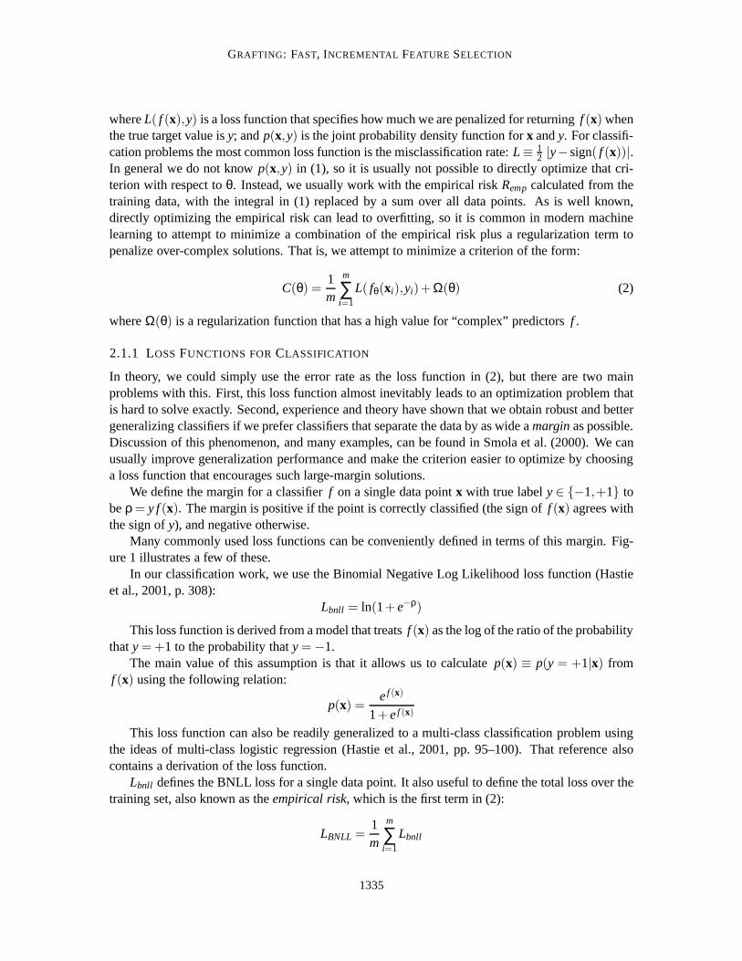
We define the margin for a classifierf on a single data pointx with true labely∈ −1,+1 tobeρ = y f(x). The margin is positive if the point is correctly classified (the sign off (x) agrees withthe sign ofy), and negative otherwise.

Many commonly used loss functions can be conveniently defined in terms of this margin. Fig-ure 1 illustrates a few of these.

In our classification work, we use the Binomial Negative Log Likelihood loss function (Hastieet al., 2001, p. 308):

Lbnll = ln(1+e−ρ)

This loss function is derived from a model that treatsf (x) as the log of the ratio of the probabilitythaty = +1 to the probability thaty =−1.

The main value of this assumption is that it allows us to calculatep(x) ≡ p(y = +1|x) fromf (x) using the following relation:

p(x) =ef (x)

1+ef (x)

This loss function can also be readily generalized to a multi-class classification problem usingthe ideas of multi-class logistic regression (Hastie et al., 2001, pp. 95–100). That reference alsocontains a derivation of the loss function.

Lbnll defines the BNLL loss for a single data point. It also useful to define the total loss over thetraining set, also known as theempirical risk, which is the first term in (2):

LBNLL =1m

m

∑i=1

Lbnll

1335


−3 −2 −1 0 1 2 30

0.5

1

1.5

2

2.5

3

3.5

4

ρf

Loss

Example Loss Functions

Error RateSVMPerceptronBinomial Negative Log Likelihood

Figure 1: Commonly used loss functions, plotted as a function of the marginρ = y f(x). Shownare the “SVM” loss function:Lsvm= max(0,1− ρ); the perceptron criterion:Lper =max(0,ρ); and the binomial negative log-likelihood:Lbnll = ln(1+e−ρ).

2.1.2 REGULARIZATION

Possibly the most straightforward approach to machine learning involves defining a family of mod-els and then selecting the model that minimizes the empirical risk. While this is certainly an often-used technique, it has two serious problems.

The first problem is that for certain combinations of model family, empirical risk function, andtraining data, the optimization problem can be unbounded with respect to the model parametersθ.For example, consider the linear model defined by:

f (x)≡n

∑i=1

wixi +b (3)

wherew = (w1, . . . ,wn)T is a vector of weights,xi is thei’th feature of the feature vectorx, andb isa constant offset. If the training data is linearly separable, then we can increase the magnitude ofwindefinitely to reduceLBNLL.

The second problem is the well-known overfitting problem. Given a sufficiently flexible familyof classifiers, it is often possible to find one that has a very low empirical risk, but that generalizesvery badly to previously unseen data.

Both these problems can be tackled by adding a regularization term to the empirical risk. Theregularization term (or regularizer) is a function of the model parameters that returns a high valuefor “unlikely” or complex models that are liable to generalize badly. By optimizing a sum of theregularizer and the empirical risk, we achieve a trade-off between model simplicity and empiricalrisk. If the balance is chosen appropriately then we can often improve generalization performancesignificantly compared with simple empirical risk minimization.

The form of the regularizer depends to some extent on the form of the model, but here we restrictourselves to a class of models where the model parametersθ take the form of a vector of real-valuednumbers of lengthp, which we will refer to as a weight vectorw. This class of models includeslinear models and many types of multi-layer perceptron (MLP).

1336


Given this parameter vector, we can define a commonly employed family of regularizers param-eterized by a non-negative integerq, and a vector of positive real numbersα:

Ωq(w) = λp

∑i=1

αi |wi |q (4)

Members of this regularizer family correspond to different kinds of weighted Minkowski normof the parameter vector, and soΩq is often referred to as anlq regularizer. Usually, we chooseαi ∈ 0,1 so as to simply include or exclude certain elements ofw from the regularization.3 Theessence of these regularizers is that they penalize large values ofwi whenαi > 0.

It is easy to show that the solutions found by unconstrained minimization of (2) using anΩq

regularizer are equivalent to those found by the following constrained optimization problem:

minimize1m

m

∑i=1

L( f (xi),yi) (5)

s.t.p

∑i=1

αi |wi |q ≤ γ

There is a one-to-one (but not necessarily simple) correspondence between the parametersλ andγ. This alternative formulation is useful when we consider theΩ0 regularizer.

The most interesting members of the family involveq∈ 0,1,2. The following is a summaryof the properties and peculiarities if these three regularizers.

Ω2 This regularizer is seen in ridge regression (Hoerl and Kennard, 1970), the support vector ma-chine (Boser et al., 1992, Sch¨olkopf and Smola, 2002) and regularization networks (Girosiet al., 1995). Those references give various justifications for this form of regularization. Onereason for preferring it over otherΩq regularizers is that it is the only one which produces thesame solution under an arbitrary rotation of the feature space axes. Thel2 norm also makesthe solution to (2) bounded. Asλ is increased, the magnitudes of the elements ofw will tendto decrease, but in general none will go to zero. Thel2 norm is a convex function of weights,and so if the loss function being optimized is also a convex function of the weights, then theregularized loss has a single local (and global) optimum.

Ω1 The l1-based regularizer is also known as the “lasso”. Tibshirani (1994) describes it in greatdetail and notes that one of its main advantages is that it often leads to solutions where someelements ofw are exactly zero. Asλ is increased, the number of zero weights steadily in-creases. Unlike theΩ2 regularizer, using thel1 norm means that an arbitrary rotation of thefeature axes in general produces a different solution, so the feature axes have special statuswith this choice of regularizer. Like theΩ2 regularizer, this regularizer leads to bounded solu-tions. Similarly, thel1 norm is a convex function of weights, and so if the loss function beingoptimized is also a convex function of the weights, then the regularized loss has a single local(and global) optimum.

Ω0 If we define 00 ≡ 0, then this contributes a fixed penaltyαi for each weightwi 6= 0. If all αi

are identical, then this is equivalent to setting a limit on the maximum number of non-zeroweights. Thel0 norm is, however, a non-convex function of weights, and this tends to makeexact optimization of (2) computationally expensive.

3. For instance in a linear model we usually want to exclude the constant offset term.

1337


2.2 Feature Selection as Regularization

If we have a mathematical expression for a model in which feature vector elements only ever appearwith an associated multiplicative weight, then the process of feature selection amounts to producinga model in which only a subset of weights associated with features are non-zero. Of the regularizersdescribed above,Ω0 andΩ1 lead to solutions with some weights set to exactly zero. But can theybe justified in terms of the standard reasons for feature selection?

There are many motivations for feature selection, but we will consider two broad classes whichgenerally encompass the reasons most commonly given.

2.2.1 PRAGMATIC MOTIVATIONS FOR FEATURE SELECTION

Often, the motivations for feature selection are pragmatic. We wish to reduce training time; reducethe time it takes to apply a learned model to new data; reduce the storage requirements for the model;or improve the intelligibility of the model. We can interpret all of these as either constituting a fixedpenalty for including a feature in the model, or as a constraint on the maximum number of featuresin the model. For the simplest linear model case, where each feature appears in the model associatedwith just a single weight, then it is easy to see that both of these interpretations correspond to aΩ0

regularizer withαi > 0 only wherewi is the multiplicative weight on a feature. For more complexmodels, where each feature might be associated with several weights, then we can handle this witha slightly modified version of theΩ0 regularizer:

Ω0(w) =n

∑i=1

αiδi (6)

whereδi = maxj∈si (w0j ), in whichsi is the set of weight indices associated with thei’th feature.

If different features carry different costs, for instance if some features are very expensive tocompute, then we can adjust theαi associated with those features accordingly.

2.2.2 PERFORMANCEMOTIVATIONS FOR FEATURE SELECTION

The other common motivation for feature selection is to improve the generalization performanceof our learned models. In general, the more feature dimensions a model includes, the greater its“capacity”, and hence the greater the tendency for it to overfit the training data — the so-called“curse of dimensionality”. But regularization techniques are intended to prevent overfitting, andthe question arises: if we use regularization, do we need to do any additional feature selection?Or alternatively, can we achieve improved generalization performance by using a regularizer thatencourages zero-weighted features in our model, such as theΩ1 andΩ0 regularizers?

In order to explore this issue, we performed a simple experiment to compare the generalizationperformance of the same simple linear classifier usingΩ0, Ω1 andΩ2 regularizers, in the presence ofvarying numbers of irrelevant features. We created a sequence of simplen-feature two-class problemas follows. For the first class, then features for each training example are drawn independently froma normal distribution with mean equal to -1 and standard deviationσ. Then features of the secondclass are generated in the same way except a normal distribution with a mean of +1 is used. We thenrandomly permute the feature values between all the training examples for all elements of the featurevector except the first two features. This produces a training set where each feature has exactly thesame distribution, but only the first two are correlated with the class label and the othern− 2

1338


0 2 4 6 8 10 120

0.05

0.1

0.15

0.2

0.25

0.3

Irrelevant features

Mea

n m

iscl

assi

ficat

ion

rate

σ=0.5

0 2 4 6 8 10 120

0.05

0.1

0.15

0.2

0.25

0.3

Irrelevant features

Mea

n m

iscl

assi

ficat

ion

rate

σ=1.0

Ω0

Ω1

Ω2

UnregularizedBayes Error

Figure 2: Comparison of different regularization schemes on a problem with varying numbers ofirrelevant features and different optimal Bayes error.

feature are irrelevant. Training sets with between 0 and 12 irrelevant features were generated, eachcontaining 10 samples drawn from each class. We compared problems withσ = 0.5 andσ = 1.0.The former has a Bayes misclassification rate of 0.0035, the latter has a Bayes misclassification rateof 0.079. Test sets were generated in the same way, but with 1000 samples in each class. We useda linear model as in (3) which was trained by optimizing a regularized risk criterion (2), using thelogistic regression loss functionLbnll and one of the threeΩq regularizers, or using no regularization.ForΩ1 andΩ2 we used a gradient descent algorithm (Nelder and Mead, 1965), and forΩ0 we usedbackward elimination (Kohavi and John, 1997), choosing to eliminate the feature that increased theloss function by the least at each step. This is a greedy procedure that may not produce the optimalanswer, but exhaustive subset comparison was impractically slow. The regularization parameters (λfor theΩ1 andΩ2 regularizers,γ for theΩ0 regularizer) were found by generating multiple instancesof each problem and searching for the values that minimized the average misclassification rate.

Figure 2 compares the performance of the various regularizers as the number of irrelevant fea-tures is altered. For each problem type, 200 training and test sets were randomly generated. Theplots show the mean test score for each type of regularizer, and for the two different values ofσ.For reasons of clarity, error bars indicating the standard error of the mean misclassification rate arenot shown here, but they are small compared to the separation between the curves.

Both values ofσ produce qualitatively similar results. The unregularized and subset selection(Ω0) experiments perform worst, although subset selection does relatively better when the informa-tive features are well-separated in the lowσ case. Of the other two experiments, when most featuresare relevant, thenΩ2 regularization slightly outperformsΩ1 regularization. But as the number ofirrelevant features increases,Ω1 regularization takes the lead. Interestingly, when more than two-thirds of the features are irrelevant in this case, the test performance usingΩ1 regularization seemsto level off, while the performance usingΩ2 regularization continues to degrade.

In conclusion, if performance alone is the key concern, then eitherΩ1 or Ω2, rather thanΩ0,seem to be the preferred regularizers. If we expect a large fraction of irrelevant features, thenwe might prefer theΩ1 regularizer. These conclusions are somewhat similar to those reached byTibshirani (1994).

1339


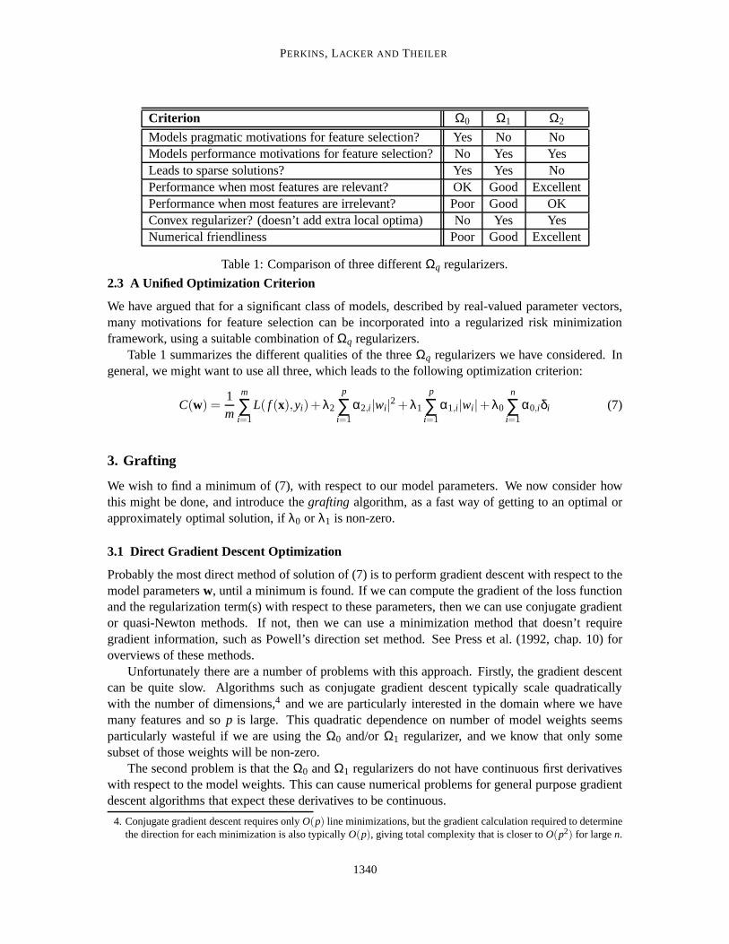
Criterion Ω0 Ω1 Ω2

Models pragmatic motivations for feature selection? Yes No NoModels performance motivations for feature selection?No Yes YesLeads to sparse solutions? Yes Yes NoPerformance when most features are relevant? OK Good ExcellentPerformance when most features are irrelevant? Poor Good OKConvex regularizer? (doesn’t add extra local optima) No Yes YesNumerical friendliness Poor Good Excellent

Table 1: Comparison of three differentΩq regularizers.

2.3 A Unified Optimization Criterion

We have argued that for a significant class of models, described by real-valued parameter vectors,many motivations for feature selection can be incorporated into a regularized risk minimizationframework, using a suitable combination ofΩq regularizers.

Table 1 summarizes the different qualities of the threeΩq regularizers we have considered. Ingeneral, we might want to use all three, which leads to the following optimization criterion:

C(w) =1m

m

∑i=1

L( f (x),yi)+ λ2

p

∑i=1

α2,i |wi|2 + λ1

p

∑i=1

α1,i |wi |+ λ0

n

∑i=1

α0,iδi (7)

3. Grafting

We wish to find a minimum of (7), with respect to our model parameters. We now consider howthis might be done, and introduce thegrafting algorithm, as a fast way of getting to an optimal orapproximately optimal solution, ifλ0 or λ1 is non-zero.

3.1 Direct Gradient Descent Optimization

Probably the most direct method of solution of (7) is to perform gradient descent with respect to themodel parametersw, until a minimum is found. If we can compute the gradient of the loss functionand the regularization term(s) with respect to these parameters, then we can use conjugate gradientor quasi-Newton methods. If not, then we can use a minimization method that doesn’t requiregradient information, such as Powell’s direction set method. See Press et al. (1992, chap. 10) foroverviews of these methods.

Unfortunately there are a number of problems with this approach. Firstly, the gradient descentcan be quite slow. Algorithms such as conjugate gradient descent typically scale quadraticallywith the number of dimensions,4 and we are particularly interested in the domain where we havemany features and sop is large. This quadratic dependence on number of model weights seemsparticularly wasteful if we are using theΩ0 and/orΩ1 regularizer, and we know that only somesubset of those weights will be non-zero.

The second problem is that theΩ0 andΩ1 regularizers do not have continuous first derivativeswith respect to the model weights. This can cause numerical problems for general purpose gradientdescent algorithms that expect these derivatives to be continuous.

4. Conjugate gradient descent requires onlyO(p) line minimizations, but the gradient calculation required to determinethe direction for each minimization is also typicallyO(p), giving total complexity that is closer toO(p2) for largen.

1340


Finally, we have the problem of local minima. TheΩ2 andΩ1 regularizers are convex functionsof the weights and so if the loss function being used is also a convex function of weights, then wehave a single optimum. TheΩ0 regularizer on the other hand is not convex and introduces manylocal minima into the optimization problem.

3.2 Stagewise Gradient Descent Optimization

If we are using theΩ1 or Ω0 regularizer, and we suspect that the numberN of non-zero weights inthe final model is going to be much less than the total number of weightsn, then a more efficientstagewise optimization procedure suggests itself. We call this algorithmgrafting. The basic plan isto begin with a model in which almost all weights are at zero. At each iteration of the grafting pro-cedure, we use a fast gradient-based heuristic to decide which zero weight should be adjusted awayfrom zero in order to decrease the optimization criterion by the maximum amount. We then performgradient descent using that weight and any other non-zero weights in the model, and continue untilno further progress can be made.

3.2.1 THE BASIC GRAFTING ALGORITHM

For ease of presentation, we first consider the case whereλ0 = 0 in (7), butλ1 andλ2 are non-zero.We will return to the case whereλ0 6= 0 later. At this stage, our discussion applies to a broad classof models and loss functions.

As described above, we assume that the model we are using is parameterized by a weight vectorw. At any stage in the grafting process, the model weights are divided into two disjoint sets. Thoseweightswi ∈ F are “free” to be altered as desired. The remaining weightswi ∈ Z(≡ ¬F ) are fixedat zero.

We also assume that the output of the model for a given training example is differentiable withrespect to the model weights,i.e.we can calculate∂ f (xi)/∂wj for an arbitrary feature vectorxi andand an arbitrary weightwj .

As explained below, after each grafting step (and before the first step) we minimize (7) withrespect to the free weights, so before thek’th grafting step, we have:

∀i ∈ F∂C∂wi

= 0

During thek’th grafting step, we wish to move one weight fromZ to F . It seems sensible toselect the weight which is going to have the greatest effect on reducing the optimization criterionC.The gradient of the criterion with respect to an arbitrary model weightwi is:

∂C∂wi

=1m

m

∑i=1

(∂L

∂ f (xi)∂ f (xi)

∂wi

)+2λ2α2,iwi + λ1α1,isign(wi)

=1m

m

∑i=1

(∂L

∂ f (xi)∂ f (xi)

∂wi

)±λ1α1,i (8)

The contribution from theΩ2 term disappears becausewi = 0 for allwi ∈Z. Slightly more subtleis the replacement of sign(wi) with ±1, which invites the question of what sign should be used, andwhether in fact sign(0) has a well-defined value at all. Recall, however, that we are interested in

1341


determining which weight, when adjusted in the appropriate direction, will decreaseC at the fastestrate. Consider∂LTOT/∂wi, the derivative of the total loss with respect towi (this is just the firstterm in the above expression). Suppose that∂LTOT/∂wi > λ1α1,i . This means that∂C/∂wi > 0,regardless of the sign ofwi . In this case, in order to decreaseC, we will want to decreasewi . Sincewi starts at zero, the very first infinitesimal adjustment towi will take it negative. Therefore for ourpurposes we can let sign(wi) = −1. Similarly, if ∂LTOT/∂wi < −λ1α1,i , then we can effectivelylet sign(wi) = +1. Essentially, the effect of theΩ1 derivative is simply to reduce themagnitudeof∂C/∂wi by an amountλ1α1,i . The same argument shows that if|∂LTOT/∂wi| < λ1α1,i then it is notpossible to produce any local decrease inC by adjustingwi away from zero. This is the essence ofwhy theΩ1 regularizer leads to solutions with zero-valued weights, and also provides the basis forone of the two stopping conditions discussed below.

At each grafting step, we calculate the magnitude of∂C/∂wi for eachwi ∈ Z, and determinethe maximum magnitude. We then add the weight to the set of free weightsF , and call a generalpurpose gradient descent routine to optimize (7) with respect to all the free weights. Since weknow how to calculate the gradient of∂C/∂wi , we can use an efficient quasi-Newton method. Weuse the Broyden-Fletcher-Goldfarb-Shanno (BFGS) variant (see Press et al. 1992, chap. 10 for adescription). We start the optimization at the weight values found in thek−1’th step, so in generalonly the most recently added weight changes significantly.

Note that choosing the next weight based on the magnitude of∂C/∂wi does not guarantee thatit is the best weight to add at that stage. However, it ismuchfaster than the alternative of tryingan optimization with each member ofZ in turn and picking the best. We shall see below that thisprocedure will take us to a solution that is at least locally optimal.

3.2.2 INCORPORATING THEΩ0 REGULARIZER

Use of theΩ0 regularizer means that transferring a weightwi from Z to F incurs a penalty ofλ0α0,iδi. This fixed penalty makes it substantially harder to determine which weight is the mostpromising one to transfer toF .5 The heuristic we use in this case is based upon the empiricalobservation that in a sequence of grafting steps, the magnitude of the most recently added weight inF typically decreases monotonically. This allows us to estimate an upper limit on the magnitude ofthe weight we are about to add, which in turn means we can roughly estimate a bound on the changein C which will result from adding a weightwi in the grafting step after a weightwj was added:

∆C(wi)≥ λ0α0,iδi −∣∣wj

∣∣(∣∣∣∣∂LTOT

∂wi

∣∣∣∣−λ1α1,i −λ2α2,i

∣∣wj

∣∣) (9)

Picking the best weight to add then amounts to choosingwi ∈ Z that minimizes (9). Note thatif λ0 = 0 and∀wi,wj ⊂ Z : α2,i = α2, j , then this heuristic is equivalent to the simple heuristicpreviously discussed.

3.2.3 STOPPINGCONDITIONS

If only the Ω2 regularizer is being used, then in general the model will contain no zero-valuedweights, and the grafting procedure will not terminate untilZ is empty. In this case there is noadvantage in using grafting over full gradient descent optimization.

5. One exception is when all weights inZ incur the sameΩ0 penalty, as is the case with a simple linear model wherewe simply penalize the number of included features. In this case it is reasonable to use the standard heuristic.

1342


If we are using theΩ1 regularizer, then we can reach a point where:

∀wi ∈ Z∣∣∣∣∂LTOT

∂wi

∣∣∣∣≤ λ1α1,i

At this point it is not possible to make any further decrease inC by either moving a weight fromZ to F , or by adjusting any weights inF and so we are at a local (and perhaps global) minimum,and can terminate the grafting procedure.

If we are using theΩ0 regularizer, then we may reach a point whereC increases after addingwi to F . We must then setwi to zero, remove it fromF , and undo the last optimization step (itis convenient to keep a copy of the previous model around in order to avoid an extra optimizationstep). We then have a choice. It is possible that a different choice ofwi might lead to a decrease inC, so we could try the optimization step again with thewi associated with the next lowest value of∆C(wi). This cycle could be repeated until all remaining weights inZ have been eliminated, andthe algorithm then terminates. Alternatively we can just terminate the algorithm the first time thishappens, recognizing that with theΩ0 regularizer, our solution will be a greedy approximation tothe optimal solution at best. The latter approach is the one we recommend in most cases.

3.2.4 OPTIMALITY

If we have a convex loss function (as a function of weights) and are using just theΩ2 and/orΩ1

regularizers (which are themselves convex functions of the weights), then there is only one minimumof (7). Examination of the stopping conditions above reveal that the grafting algorithm is guaranteedto stop at a local optimum, and so grafting is guaranteed to find the global optimum in these cases.

As we have seen by now, use of theΩ0 regularizer makes it much harder to find an optimalsolution. The grafting procedure with non-zeroλ0 amounts to a greedy heuristic forward subset se-lection method, which sacrifices optimality in return for fast learning. Whether this is good enoughfor the problem at hand depends on the situation.

One should note however, that asλ0 is made smaller and smaller relative toλ1, then the chancesof ending up in a sub-optimal situation decrease. Hence we are inclined to makeλ0 fairly small inmost cases.

3.2.5 COMPUTATIONAL COMPLEXITY

We have claimed that grafting is substantially faster than full gradient descent. We will now exam-ine this claim more carefully. If there arep weights in our weight vector, then full gradient descentrequires some multiple ofp line minimizations to optimize our criterion, let’s saycp minimiza-tions.6 Determining the direction requiresp derivatives∂C/∂wi to be computed. The computationof each derivative is dominated by the computation of∂LTOT/∂wi , which is simply a weighted sumof m simple derivatives∂ f (x j)/∂wi . The line minimizations themselves require a fewO(m) func-tion evaluations, but ifp is large, then this is a minor contribution. If we denote the time taken tocalculate one simple derivative asτ, then the total time taken for full gradient descent is≈ cmp2τ.

Under grafting we will select some numbers weights before the algorithm terminates. Sincewe select one weight at each grafting step we takes steps. Thek’th step consists of two phases.First we evaluate∂C/∂wi for each of the(p− k) weights inZ. As noted above, the derivativecalculation takesmτ, and so the time devoted to gradient testing overs steps is≈ mspτ. The

6. Here,c = 1 if our criterion is a perfect quadratic form, andc > 1 otherwise.

1343


second phase involves optimizing with respect to thek free weights. At most this might takeckline minimizations, but it should take less than this since most of the free weights will be close totheir optimal values. To compensate for using a constantc that is probably too high here, we againignore the time taken for the line minimizations themselves (some small multiple ofmτ). Thereforethe time taken for optimization at thek’th step is≈ cmk2τ. Overs steps, this is≈ 1

3cms3τ. Puttingthis together the total grafting run time is≈ (msp+ 1

3cms3)τ. If we assume thats p then it isclear that the grafting algorithm should be substantially quicker than the≈ cmp2τ required for fullgradient descent. Also note that the full gradient descent algorithm has to deal with discontinuitiesin the gradient which can slow it down significantly. By keeping zero-valued weights out of theoptimization steps, grafting avoids this difficulty.

3.2.6 NORMALIZATION

In order to make the gradient magnitude heuristic a fair comparison, it is usually important tonormalize all features so that they have approximately the same scale. Before we begin, we linearlyscale all feature vectors so that each feature has a mean value of zero and has a standard deviation ofone. It is of course important to scale testing data using the same scaling parameters derived fromthe training data.

3.3 Grafting Examples

It is helpful to illustrate the grafting algorithm in more detail for some particular models and lossfunctions. Here we will concern ourselves only with binary classification problems and so a suitableloss function to use is the binomial negative log likelihoodLbnll . For simplicity, we will also assumeonly Ω1 andΩ0 regularization are used, and that allα1,i ∈ 0,1.

3.3.1 LINEAR MODEL

We first consider linear models withn+1 weights, of the form:

f (x) =n

∑i=1

wixi +w0

If we define the margin for a given training pair(xi ,yi) asρi = yi f (xi), then the following is theregularized optimization criterion:

C(w) =1m

m

∑i=1

(1+e−ρi )+ λ1

n

∑i=1

|wi|+ λ0s (10)

wheres is the number of selected features. Note that the constant offset termw0 does not appear inthe regularizer since we do not want to penalize a mere translation of the linear discriminant surface.

The derivatives we need (ignoring theΩ0 term for now) are:

∂C∂wj

=1m

m

∑i=1

∂Lbnll

∂ρi

∂ρi

∂wj±λwj

= − 1m

m

∑i=1

11+eρi

yixi, j ±λwj

wherexi, j is the j ’th component ofxi .

1344


It is instructive to interpret this derivative in a geometric way. First, we imagine anm-dimensionalmargin space, which has one dimension for each training point. If we think of each of the coor-dinate axes as representing the marginsρi for the current model on the pointxi , then the total lossfunction can be thought of as a function over this space, and we can calculate the full gradient ofthat function:

∇ρL =(

∂L∂ρ1

,∂L∂ρ2

, . . . ,∂L

∂ρm

)T

In the same margin space we can also imagine thefeature margin vectorr j :

r j = (y1x1, j ,y2x2, j , . . . ,ymxm, j)T

Given this we can write:∂C∂wj

= ∇ρL · r j ±λwj

Since the grafting heuristic for selecting the next weight to add to the model is only interestedin the magnitude of this derivative, and since the regularizer component always acts to reduce thismagnitude, we can see that picking the next weight amounts to choosing the feature margin vectorthat is most well-aligned with the direction of steepest descent of the loss function in margin space.

For the linear model, we initializeF to contain justw0 and perform an initial optimization. Wethen proceed in the usual grafting fashion, picking one new weight to add toF at each graftingstep until anΩ0 or Ω1 stopping condition is reached. In this case, each weight corresponds to onefeature.

The simplicity of the linear model means that it sometimes cannot fit the training data verywell. But this problem is somewhat reduced when we have many features since in general the extrafeatures will tend to make the problem more linearly separable.

3.3.2 MULTI LAYER PERCEPTRONMODEL

For a more powerful model, we might use an MLP withh hidden units having sigmoid transferfunctions and a linear output unit with unit output weights. We can write this MLP function as:

f (x) =h

∑j=1

g

(n

∑i=1

w( j)i xi +w( j)

0

)+w(0)

0

In this modelw( j)i is the weight from thei’th feature to thej ’th hidden unit. The sigmoid transfer

functiong(·) is defined as:

g(x) =2

1+e−x −1

which is the usual neural net sigmoid function, scaled vertically so thatg(0) = 0, g(+∞) = +1 andg(−∞) =−1, which makes the net slightly better behaved under grafting.

The optimization criterion is almost identical to (10) with the differentf (·) substituted. All theweights in the MLP model are included equally in the regularization term, except for the “bias”weights on each node which are excluded, and the constant weights on the output node. Rather thanuse a fixed number of hidden units, the grafting procedure we describe here allows hidden units tobe added as the grafting process continues. In the MLP model, each weight added corresponds to

1345


a new connection in the network. We begin withF containing just the output bias weightw(0)0 and

a network with no hidden units, and perform an initial optimization with respect to just that biasweight. At each grafting step we decide how to grow the network in one of two possible ways:

Adding a new hidden unit: If there arek−1 hidden units already, this involves adding a hiddennode, along with a new connection to the output node, and a new connection from the hidden nodeto a feature input, with weightw(k)

i . The question becomes: which feature should be connected tothe new hidden unit? The derivative we need is:

∂C

∂w(k)i

=− 1m

m

∑j=1

11+eρi

yjxj,i ±λw(k)i

Adding an input connection to an existing hidden unit: Each of theh hidden units may beconnected to any of then input features and any of these connections are candidates for adding tothe model (if they are not present already). If we are considering adding a connection from thei’thinput feature to thek’th hidden unit, then the relevant derivative is:

∂C

∂w(k)i

=− 1m

m

∑j=1

11+eρi

yj xj,i g′(

n

∑l=1

w(k)l xi,l +w(k)

0

)±λw(k)

i

with:

g′(x) =2e−x

(1+e−x)2

After t grafting steps, there aren possibilities to consider for adding a new hidden unit, and(hn− t) possibilities to consider for adding a connection to a new hidden unit. Following the usualgrafting procedure, we calculate the derivatives for all these candidates and pick the one with thelargest magnitude. The corresponding weight is added toF and we reoptimize. The cycle isrepeated until one of the stopping conditions is met. If a new hidden unit is added, then we alsoneed to include the associated bias weight, initialized at zero, inF .

3.4 Variants

A number of variants to the basic grafting procedure are possible. One interesting alternative isnot to attempt a full optimization of the full setF after each grafting step. Instead only the mostrecently added weight and perhaps the bias weights are adjusted. This makes each grafting stepfaster, at the expense of a loss in accuracy and the strong possibility of ending up at a solution that isnot even a local optimum. In practice, if only a small fraction of the possible weights are non-zerowhen grafting finishes, then the time spent checking gradients to determine the next weight to addoften dominates the run time, and so saving a little effort on the optimization makes little difference.

Grafting can also be readily extended to regression problems through the use of a suitable lossfunction, such as the squared error loss function. This has not yet been implemented.

4. Grafting Experiments

In this section, we compare the performance of grafting and a number of other different approachesto feature selection, on a set of synthetic and real world test problems. For simplicity, we concentrateentirely on binary classification problems in this paper.

1346


4.1 The Datasets

Five datasets were used in these experiments, labeledA throughE. Each dataset consists of a train-ing set and a test set. DatasetsA, B andC are synthetic problems, and are all instances of the samebasic task described below. DatasetsD andE are real world problems, taken from the online UCIMachine Learning Repository (Blake and Merz, 1998).

The three synthetic problems are variations of a task we call thethreshold max(TM) problem.In the most basic version of this problem, the feature space containsnr informative features, each ofwhich is uniformly distributed between -1 and +1. The output label for a given point is defined as:

y =

+1 if max(xi) > 2(1−1/nr ))−1 ; i = 1. . .nr

-1 Otherwise

The y = −1 points occupy a large hypercube wedged into one corner of the larger hypercubecontaining all the points. They = +1 points fill the remaining space. The constant in the aboveexpression is chosen so that half the feature space belongs to each class. Variations of this basicproblem are derived by addingni irrelevant features uniformly distributed between -1 and +1, andnc redundant features which are just copies of the informative features. The TM problem is designedso that each of the informative features only provides a little information, but by using all of themtogether, the problem is completely separable. In addition, the optimal discriminating surface forthe problem is very non-linear, but the problem is asymmetric so a linear discriminant should beable to do at least better than random.

Ten instantiations of the training and testing sets of each of the three synthetic problems weregenerated to obtain some statistics on relative algorithm performance.

In more detail, the datasets are:

Dataset A The TM problem, withnr = 10, nc = 0 andni = 90. Both the training set and thetest set contain 1000 points each. This dataset explores the effect of irrelevant features in the TMproblem.

Dataset B The TM problem, withnr = 10, nc = 90 andni = 0. Both the training set and thetest set contain 1000 points each. This dataset explores the effect of redundant features in the TMproblem.

Dataset C The TM problem, withnr = 10,nc = 490 andni = 500. The training set contains only100 training points, despite the problem dimensionality of 1000. The test set contains 1000 points.This dataset explores an extreme situation in which there are many more features than trainingpoints.

Dataset D The “Multiple Features” database from the UCI repository. This is actually a handwrit-ten digit recognition task, where digitized images of digits have been represented using 649 featuresof various types. The task tackled here is to distinguish the digit “0” from all other digits. Thetraining and test sets both consist of 1000 points. The features were all scaled to have zero meanand unit variance before being used here.

Dataset E The “Arrhythmia” database from the UCI repository. The task here is to distinguishnormal from abnormal heartbeat behavior from ECG data described by 279 numeric and binaryattributes. The data was slightly modified from the original to make it easier to use. Feature number14 (“J”) was missing in most of the records, so it was removed from all the records. Of the 452

1347


instances in the database, 32 had other missing attribute values and so those instances were alsoremoved, leaving 420 instances described by 278 attributes. These were divided into a training setof 280 points, and a test set of 140 points.

All the datasets used in these experiments can be found online at:

http://nis-www.lanl.gov/˜simes/data/jmlr02/

4.2 The Algorithms

Eight different algorithms, which we denote by the letters(a) through(h), were compared on thefive datasets described above. Except where described below, all implementation relied on Matlab(including the Matlab Optimization Toolbox).

(a) The linear grafting algorithm described in Section 3.3, and using bothΩ0 andΩ1 regularization.

(b) The MLP grafting algorithm described in Section 3.3, and using bothΩ0 andΩ1 regularization.

(c) Simple gradient descent to fit anΩ1 regularized linear combination of all the input features.After gradient descent is complete, any weights with a magnitude less than 10−4 of the maxi-mum magnitude in the weight vector, are pruned in order to obtain the subset selection drivenby theΩ1 regularization.

(d) Simple gradient descent to fit anΩ1 regularized, fully connected MLP of a similar form tothat learned by the MLP grafting algorithm, with the exception that the number of hiddennodes is fixed at 10 nodes (and of course the connectivity is much higher). After gradientdescent is complete, any weights with a magnitude less than 10−4 of the maximum magnitudein the weight vector, are pruned in order to obtain the subset selection driven by theΩ1

regularization.

(e) Linear SVM, which effectively usesΩ2 regularization and a slightly different loss function thanthat used by the grafting implementations. The SVM implementation we used islibsvm(Chang and Lin, 2001).

(f) Gaussian RBF kernel SVM, using the defaultlibsvm kernel parameters.

(g) Gaussian RBF kernel SVM as above, but in conjunction with “wrapper” feature subset selection.At each feature selection step, all possible features are considered for addition to the currentfeature set, and 3-fold cross-validation is used to select the best one. This process is repeateduntil we have selected 10 features, and a final RBF SVM is trained using just those features.This is essentially greedy forward subset selection.

(h) Gaussian RBF kernel SVM, but in conjunction with a “filter” feature subset selection. For eachdataset, we simply take the 10 features that are most highly correlated with the label and trainour SVM using those features.

Note that an efficient implementation of grafting must directly exploit the sparsity of the modelsbeing trained. Our Matlab implementations take care to do this.

1348


Linear Graft/GD MLP Graft/GD Linear SVM RBF SVM(λ1/λ0) (λ1/λ0) (C) (C)

A 3×10−4/0.005 10−6/0.005 0.01 10B 10−4/0.005 10−6/0.005 0.01 0.1C 0.2/0.001 0.1/0.001 0.001 100D 0.005/0.001 3×10−4/0.001 1 1E 0.05/0.001 3×10−5/0.001 0.01 1

Table 2: Regularization parameters used in experiments for each dataset, chosen using five-foldcross-validation. “GD” stands for Gradient Descent.

4.3 Experimental Details

Each algorithm was applied to each of the datasets. The exception to this was the fully connectedMLP (algorithm (d)), which failed to converge for several of the larger datasets. We suspect thatthis was caused by the large number of weights close to zero in the model, and the discontinuousderivative of the regularizer at this point. For the three synthetic problems the training runs wererepeated for ten different random instantiations of the training and test sets, to assess sensitivity tosmall changes in the dataset.

The regularization parameters used in these experiments were chosen using five-fold cross val-idation on each of the training sets. Algorithms(a) and(c) share the same parameters; as do algo-rithms (b) and(d); and algorithms(f), (g) and(h). Note that the grafting algorithms,(a) and(b),use bothΩ1 andΩ0 regularization, requiring parametersλ1 andλ0, while the corresponding simplegradient descent algorithms,(c) and (d), use onlyΩ1 regularization. This is due to the difficultyof incorporatingΩ0 regularization into a standard gradient descent algorithm. The parameters arelisted in Table 2.

For the Matlab implementations (algorithms(a), (b), (c) and (d)) the training time on eachdataset was recorded to see if grafting gave a speedup over simple gradient descent. A direct speedcomparison between the SVM algorithms (written in C) and the Matlab implementations was notattempted at this time, due to the inherent efficiency differences between Matlab and C code.

We also recorded the number of features selected (not the same as the number of weights ingeneral), for those algorithms that select a subset of the features (all algorithm except(e) and(f)).In addition, for the three synthetic problems, we can directly calculate a measure of how useful theselected feature subsets are. Recall that in each of these problems there arenr informative features,not including redundant duplicates. We can define a feature setsaliencymeasure:

s=ng

nr+

ng

nf−1

whereng is the number of “good” features selected (i.e. informative features, but not includingany duplicate redundant features), andnf is the total number of features selected. The saliencyevaluates to 1 if allnr good features are selected and no others are selected. It evaluates to -1 ifno good features are selected, and it evaluates to approximately zero if all the good features areselected, but only along with many irrelevant or redundant features.

Note that the number of selected features for the linear and MLP models trained by simplegradient descent (algorithms(c) and (d)) relies on a somewhat subjective pruning of low valuedweights, as described above. Therefore the measurements of numbers of selected features, and

1349


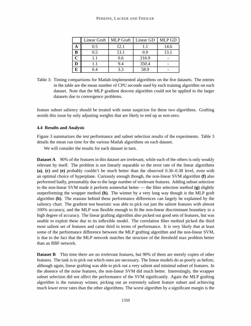
Linear Graft MLP Graft Linear GD MLP GD

A 0.5 12.1 1.1 14.6B 0.5 13.1 0.9 13.1C 1.1 0.6 216.9 -D 1.1 9.4 350.4 -E 0.4 3.3 58.9 -

Table 3: Timing comparisons for Matlab-implemented algorithms on the five datasets. The entriesin the table are the mean number of CPU seconds used by each training algorithm on eachdataset. Note that the MLP gradient descent algorithm could not be applied to the largerdatasets due to convergence problems.

feature subset saliency should be treated with some suspicion for these two algorithms. Graftingavoids this issue by only adjusting weights that are likely to end up as non-zero.

4.4 Results and Analysis

Figure 3 summarizes the test performance and subset selection results of the experiments. Table 3details the mean run time for the various Matlab algorithms on each dataset.

We will consider the results for each dataset in turn.

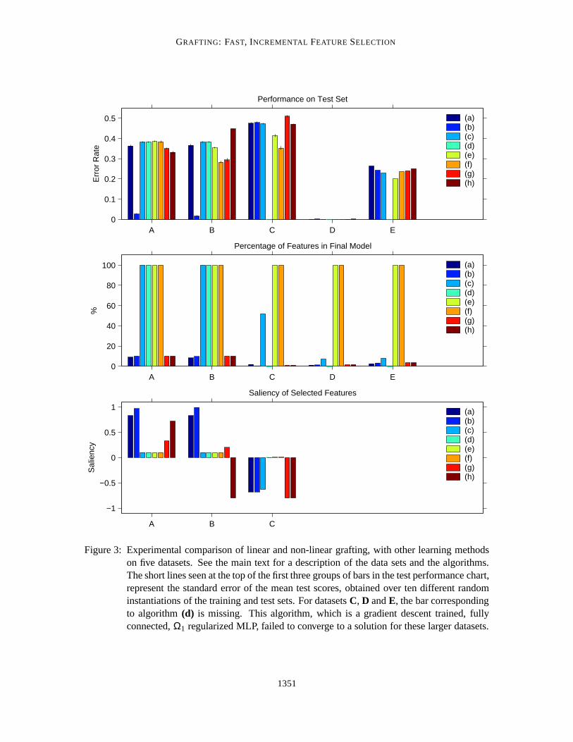
Dataset A 90% of the features in this dataset are irrelevant, while each of the others is only weaklyrelevant by itself. The problem is not linearly separable so the error rate of the linear algorithms(a), (c) and (e) probably couldn’t be much better than the observed 0.36–0.38 level, even withan optimal choice of hyperplane. Curiously enough though, the non-linear SVM algorithm(f) alsoperformed badly, presumably due to the large number of irrelevant features. Adding subset selectionto the non-linear SVM made it perform somewhat better — the filter selection method(g) slightlyoutperforming the wrapper method(h). The winner by a very long way though is the MLP graftalgorithm (b). The reasons behind these performance differences can largely be explained by thesaliency chart. The gradient test heuristic was able to pick out just the salient features with almost100% accuracy, and the MLP was flexible enough to fit the non-linear discriminant boundary to ahigh degree of accuracy. The linear grafting algorithm also picked out good sets of features, but wasunable to exploit these due to its inflexible model. The correlation filter method picked the thirdmost salient set of features and came third in terms of performance. It is very likely that at leastsome of the performance difference between the MLP grafting algorithm and the non-linear SVM,is due to the fact that the MLP network matches the structure of the threshold max problem betterthan an RBF network.

Dataset B This time there are no irrelevant features, but 90% of them are merely copies of otherfeatures. The task is to pick out which ones are necessary. The linear models do as poorly as before,although again, linear grafting was able to pick out a very salient and minimal subset of features. Inthe absence of the noise features, the non-linear SVM did much better. Interestingly, the wrappersubset selection did not affect the performance of the SVM significantly. Again the MLP graftingalgorithm is the runaway winner, picking out an extremely salient feature subset and achievingmuch lower error rates than the other algorithms. The worst algorithm by a significant margin is the

1350


A B C D E0

0.1

0.2

0.3

0.4

0.5

Err

or R

ate

Performance on Test Set

(a)(b)(c)(d)(e)(f)(g)(h)

A B C D E0

20

40

60

80

100

%

Percentage of Features in Final Model

(a)(b)(c)(d)(e)(f)(g)(h)

A B C

−1

−0.5

0

0.5

1

Sal

ienc

y

Saliency of Selected Features

(a)(b)(c)(d)(e)(f)(g)(h)

Figure 3: Experimental comparison of linear and non-linear grafting, with other learning methodson five datasets. See the main text for a description of the data sets and the algorithms.The short lines seen at the top of the first three groups of bars in the test performance chart,represent the standard error of the mean test scores, obtained over ten different randominstantiations of the training and test sets. For datasetsC, D andE, the bar correspondingto algorithm(d) is missing. This algorithm, which is a gradient descent trained, fullyconnected,Ω1 regularized MLP, failed to converge to a solution for these larger datasets.

1351


filter-based subset selection technique. This is to be expected since this simple filter has no reasonnot to pick multiple redundant features.

Dataset C With 1000 dimensions and only 100 training points this is a very hard problem. Look-ing at the saliency chart, it is clear that the grafting algorithms, along with both the wrapper and filterselection methods, pick out very poor subsets of features. The only algorithms to perform much bet-ter than a random classifier are the two SVM algorithms without subset selection,(e) and(f). Thenon-linear SVM performs best by a significant margin. The problem seems to be that, given enoughfeatures and few enough data points, the grafting and other subset selection methods are very likelyto find irrelevant features that explain the labels better than the true informative features, merely bychance. They then seize on those features as the most useful. In contrast, the basic SVM, withl2regularization and no subset selection, has less tendency to focus on just a few features, and so doesbetter.

Dataset D The digit recognition problem turns out to be very easy, with most algorithms misclas-sifying only one member of the test set, out of 1000. The challenge here is to solve the problemquickly and using as few features as possible — many of the features are relatively expensive tocompute so this is a real-world challenge. The linear and non-linear grafting algorithms(a) and(b) do an excellent job in this respect, achieving excellent performance using only about 1% of thefeatures. This parsimony also pays off in terms of training time, as the linear grafting algorithm isover 300 times faster than training a full linear model using gradient descent.

Dataset E The arrhythmia problem is quite a hard one. The best algorithm is the linear SVM(e),with an average error rate of around 0.2. All the other algorithms achieve performance figures in thevicinity of 0.25, although the grafting algorithms achieve this error rate using a very small fractionof the available features.

5. Discussion

We finish with some conclusions, and compare grafting to some better-known algorithms.

5.1 Connections with Stagewise Additive Modelling

Both the linear and MLP models considered in this paper are examples of additive models:

E(y|x) =k

∑i=1

fi(x)

Hastie et al. (2001, chap. 9) provide an in-depth discussion of this class of models which have along history in statistics. They also describe a method called additive regression that allows us to fitthe above model usingbackfitting(Friedman and Stuetzle, 1981). Backfitting is a simple iterativeprocedure whereby the individual functionsfi are adjusted one at a time to optimize a chosen lossfunction, and by cycling through this process enough times we can optimize the whole model. Ad-ditive logistic regression specializes this problem for classification by using the binomial negativelog likelihood loss function as an optimization criterion. For the classes of additive model consid-ered in this paper, we can simply use sophisticated general purpose gradient descent algorithms tooptimize the model, which are likely to be more efficient than the simple backfitting procedure.

1352


As an alternative to using a model with a fixed number of componentsk, we can incrementallydevelop such a model using a greedy stagewise algorithm. In this approach, at each time step, weadd a new component to the additive model, which is designed to reduce the current loss as muchas possible. The previous components are fixed, and only the new function is adjusted. An exampleof this ismatching pursuit, described by Mallat and Zhang (1993). This approach is also discussedat length by Friedman et al. (2000) where they develop a greedy stagewise form of additive logisticregression.

All this looks very similar to the grafting procedure described in this paper, so what is new aboutgrafting? Here are some of the more important differences:

• Grafting is used to build up models out of components that may be combined together inmuch more complicated ways than simply being added together. In MLP graft, for instance,at each grafting step we consider both adding a new hidden node, and adding an input to anexisting node. These options are considered in the same framework, but involve rather differ-ent alterations to the model. In stagewise additive modelling we are usually only concernedwith adding anotherfi to the model at each step.

• At each step, grafting considers many possibilities for altering the current model (typicallyone for each weight inF ) and decides between them using the gradient test heuristic. Instagewise additive modelling, we usually only consider one possibility, which is to add (liter-ally) a new functionfi , which will be fit to a weighted version of the training set.

• After updating the model, stagewise additive modelling typically only adjusts parametersrelating to the most recently addedfi. Grafting usually adjusts all the free parameters inthe model using a gradient descent engine. This is feasible because our model output isalways differentiable with respect to all the model parameters. Additive model practitionersdo sometimes use backfitting to fit their models, but this is likely to be less efficient than usinga quasi-Newton gradient descent algorithm.

5.2 Connections with Boosting

Boosting (Freund and Schapire, 1996) is one of the most active fields of research in modern machinelearning. Boosting, and in particular the AdaBoost algorithm, provides a way of training a sequenceof classifiers on some data and then combining them together to form anensemble classifierthat issubstantially better than any of its member classifiers.

Boosting can be viewed as a form of stagewise additive modelling (Friedman et al., 2000) thatoptimizes a logistic regression-like loss function, combined with anl1 regularizer. It works byreweighting the training data at each stage, training a new classifier using a “weak learner”, andforming a composite classifier as a linear combination of the classifiers learned at each stage. Thereweighting of the data can be shown to “encourage” a new classifier to be learned that maximallydecreases the logistic regression loss (Friedman et al., 2000).

If we consider the variant of grafting mentioned in Section 3.4, where we only update the mostrecently added weights, and use a linear model withΩ1 regularization, then we end up with some-thing that is very much like an extreme version of boosting where the weak learner simply fits amodel of the formf (x) = w0 + w1xk, choosing a single featurexk to add to the model. The tech-nique of “boosting with stumps” is similar to this, except thatf (x) is usually thresholded at zeroto produce an output that is -1 or +1, as required by the original AdaBoost algorithm. More recent

1353


versions of boosting relax this requirement (Schapire and Singer, 1999) however, so in fact thisvariant of linear grafting is a simple form of boosting.

The original boosting algorithm mandated anl1 regularizer and the logistic regression loss func-tion. However, Mason et al. (2000) have devised a general purpose algorithm called AnyBoost,which, like grafting (and stagewise additive modelling) can work with a variety of loss functionsand regularization methods.

5.3 Implications for Regularization

We achieved best performance with the grafting algorithms using both aΩ1 and aΩ0 regularizer. Ithas been argued, (e.g., see Tibshirani, 1994), thatΩ1 regularization represents a good compromisebetween the needs of coefficient shrinkage for generalization performance, and the needs of subsetselection for pragmatic reasons. However, as discussed in Section 2.1.2, these are really two separategoals and perhaps should be accounted for separately. Our experience is that if we attempted to useonly Ω1 regularization then it was often impossible to find a single value ofλ1 that produced goodgeneralization performance without also incorporating many largely irrelevant features. It shouldbe noted, though, that theΩq regularizer withq = 1 is the smallestq-value where the regularizer isconvex.

5.4 Other Related Work

Das (2001) describes a technique for using boosting for feature selection. However he does notcombine feature selection with model building in the integrated way we have described.

Jebara and Jaakkola (2000) also examine feature selection in a regularized risk minimizationcontext for linear models. They define a prior describing likely values of weights, and choose onethat tends to drive a number of weights to zero, in a similar fashion tol1 regularization. In factl1 regularization can be viewed as being equivalent to a sharply peaked prior for weight values(Tibshirani, 1994).

Weston et al. (2000) describe a gradient descent method that can be used to select a subset offeatures non-linear for support vector machines. The input features are first weighted using a vectorof weightsσ. This vector is then optimized using gradient descent, to minimize a bound on theexpected leave-one-out error, subject to al1 constraint on the magnitude ofσ. This leads to some ofthe elements ofσ being driven to zero.

SVMs are normally associated withl2 regularization, but it is possible to formulate them usingan l1 norm as well. Fung and Mangasarian (2002) describe a gradient descent technique for rapidlyoptimizing suchl1 SVMs, which have the property that, as usual, many weights are driven to zero.

References

C.L. Blake and C.J. Merz. UCI repository of machine learning databases.http://www.ics.uci.edu/˜mlearn/MLRepository.html , 1998. University of Califor-nia, Irvine, Dept. of Information and Computer Science.

B. Boser, I. Guyon, and V. Vapnik. A training algorithm for optimal margin classifiers. InProc.Fifth Annual Workshop on Computational Learning Theory, pages 144–152, Pittsburgh, ACM,1992.

1354


C. Chang and C. Lin. LIBSVM: A library for support vector machines. Software available athttp://www.csie.ntu.edu.tw/ cjlin/libsvm , 2001.

S. Das. Filters, wrappers and a boosting-based hybrid for feature selection. InProc. ICML. MorganKauffmann, 2001.

Y. Freund and R.E. Schapire. Experiments with a new boosting algorithm. InMachine Learning:Proc. 13th Int. Conf., pages 148–156. Morgan Kaufmann, 1996.

J. Friedman, T. Hastie, and R. Tibshirani. Additive logistic regression: A statistical view of boosting.Annals of Statistics, 28:337–307, 2000.

J. Friedman and W. Stuetzle. Projection pursuit regression.Journal of the American StatisticalAssociation, 76:817–823, 1981.

G. Fung and O.L. Mangasarian. A feature selection Newton method for support vector machineclassification. Technical Report 02-03, Data Mining Institute, Dept. of Computer Sciences, Uni-versity of Wisconsin: Madison, Sept 2002.

F. Girosi, M. Jones, and T. Poggio. Regularization theory and neural networks architectures.NeuralComputation, 7:219–269, 1995.

T. Hastie, R. Tibshirani, and J. Friedman.The Elements of Statistical Learning. Springer, 2001.

A.E. Hoerl and R. Kennard. Ridge regression: Biased estimation for nonorthogonal problems.Technometrics, 12:55–67, 1970.

T. Jebara and T. Jaakkola. Feature selection and dualities in maximum entropy discrimination. InProc. Int. Conf. on Uncertainity in Artificial Intelligence, 2000.

K. Kira and L. Rendell. A practical approach to feature selection. In D. Sleeman and P. Edwards,editors,Proc. Int. Conf. on Machine Learning, pages 249–256. Morgan Kaufmann, 1992.

R. Kohavi and G.H. John. Wrappers for feature subset selection.Artificial Intelligence, 97:273–324,1997.

S. Mallat and Z. Zhang. Matching pursuit with time-frequency dictionaries.IEEE Transactions onSignal Processing, 41(12):3397–3415, 1993.

L. Mason, J. Baxter, P.L. Bartlett, and M. Frean. Functional gradient techniques for combininghypotheses. In A.J. Smola, P.L Bartlett, B. Sc¨olkopf, and D. Schuurmans, editors,Advances inLarge Margin Classifiers, pages 221–246. MIT Press, 2000.

J.A. Nelder and R. Mead. A simplex method for function minimization.Computer Journal, 7:308–313, 1965.

W.H. Press, S.A. Teukolsky, W.T. Vetterling, and B.P. Flannery.Numerical Recipes in C. CambridgeUniversity Press, 2nd edition, 1992.

R.E. Schapire and Y. Singer. Improved boosting algorithms using confidence-rated predictions.Machine Learning, 37(3):297–336, 1999.

1355


B. Scholkopf and A. Smola.Learning with Kernels. MIT Press, Cambridge, MA, 2002.

A.J. Smola, P.J. Bartlett, B. Sch¨olkopf, and D. Schuurmans, editors.Advances in Large MarginClassifiers. MIT Press, 2000.

R. Tibshirani. Regression shrinkage and selection via the lasso. Technical report, Dept. of Statistics,University of Toronto, 1994.

J. Weston, S. Mukherjee, O. Chapelle, M. Pontil, T. Poggio, and V. Vapnik. Feature selection forSVMs. Advances in Neural Information Processing Systems, 13, 2000.

1356

Grafting: Fast, Incremental Feature Selection by Gradient...

Documents

Transcript of Grafting: Fast, Incremental Feature Selection by Gradient...