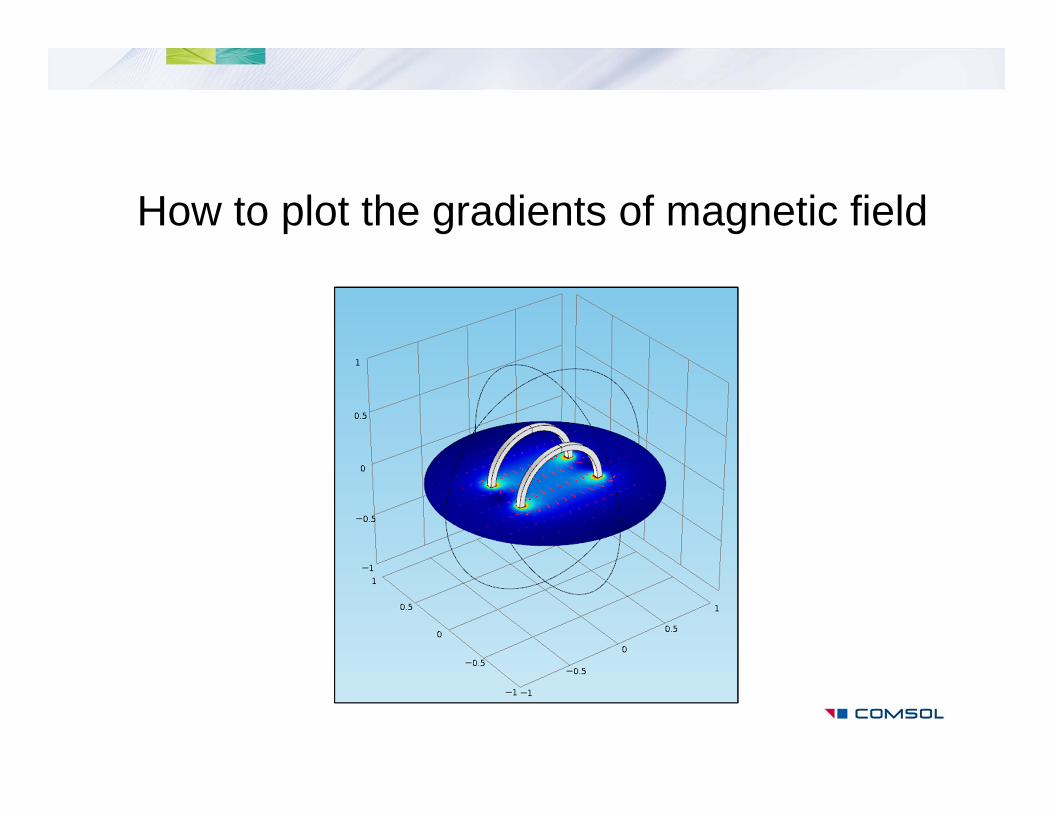
How to plot the gradients of magnetic field

• 3D magnetic problems are solved in COMSOL using vector (curl) elements.

• The solution to these problems is the magnetic vector potential (A).

• The magnetic flux density (B) involves the 1st derivative of A and is given by the following equation.

• The second derivative is not defined on vector elements and hence we cannot visualize spatial gradients of B directly in COMSOL.

Background

AB

• This tutorial shows how to visualize the spatial derivatives of B.

• The technique demonstrated here shows how each component of B = [Bx, By, Bz] can mapped to a separate variable say u, u2, u3 respectively.

• These new variables would be defined on Lagrange elements.

• Since both 1st and 2nd order derivatives are defined on Lagrange elements, we would be able to obtain spatial derivatives of each component of B.

• The mapping on Lagrange elements will also allow the use of polynomial patch recovery to get smooth values of derivatives.

Objective

Modeling steps

• The next few slides illustrate the steps involved in mapping the solution from an existing 3D magnetic model.

• The detailed steps are available in the file: helmholtz_coil_field_gradient_42a

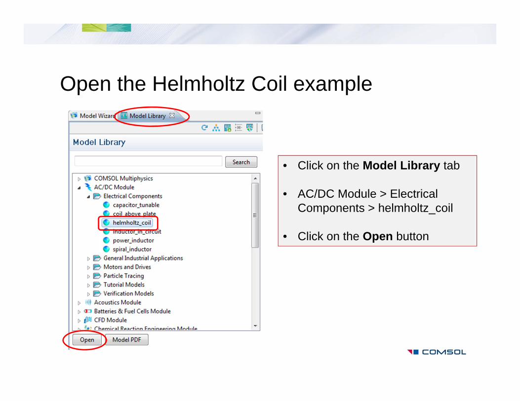
Open the Helmholtz Coil example

• Click on the Model Library tab

• AC/DC Module > Electrical Components > helmholtz_coil

• Click on the Open button

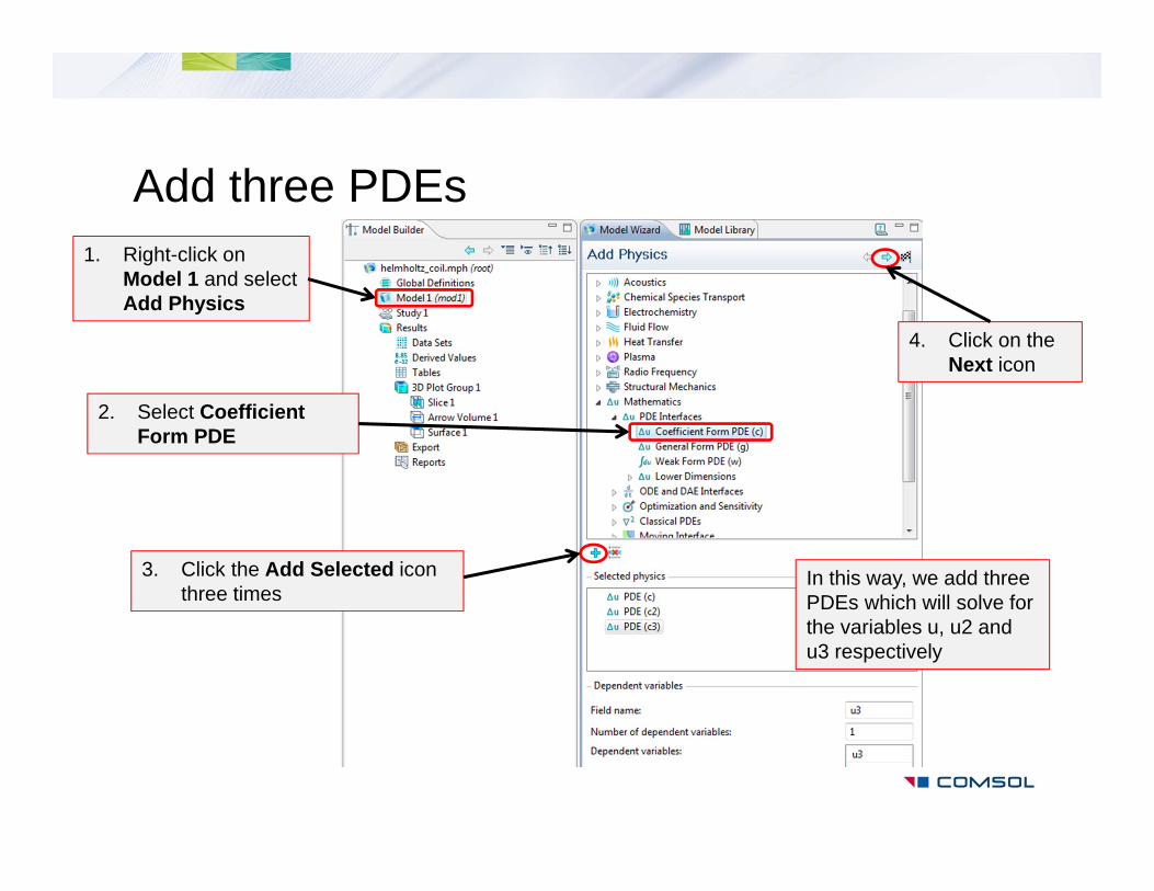
Add three PDEs

2. Select Coefficient Form PDE

1. Right-click on Model 1 and select Add Physics

3. Click the Add Selected icon three times

In this way, we add three PDEs which will solve for the variables u, u2 and u3 respectively

4. Click on the Next icon

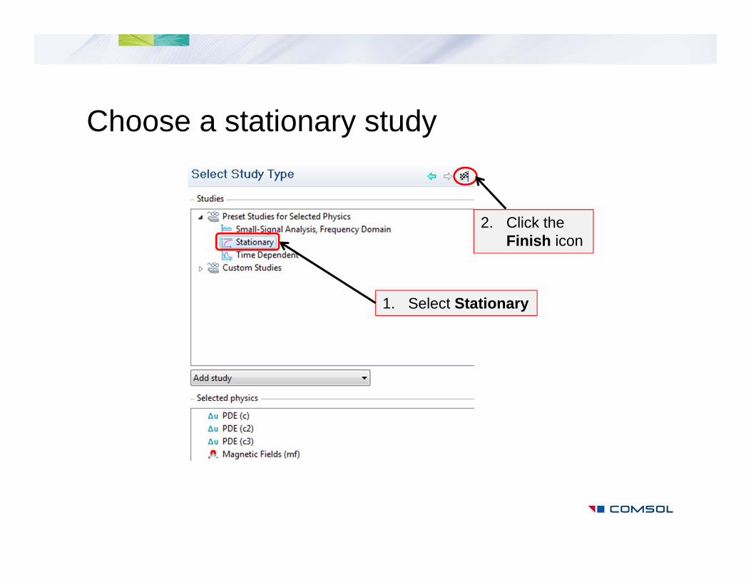
Choose a stationary study

1. Select Stationary

2. Click the Finish icon

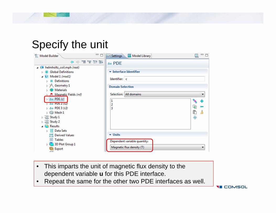
Specify the unit

• This imparts the unit of magnetic flux density to the dependent variable u for this PDE interface.

• Repeat the same for the other two PDE interfaces as well.

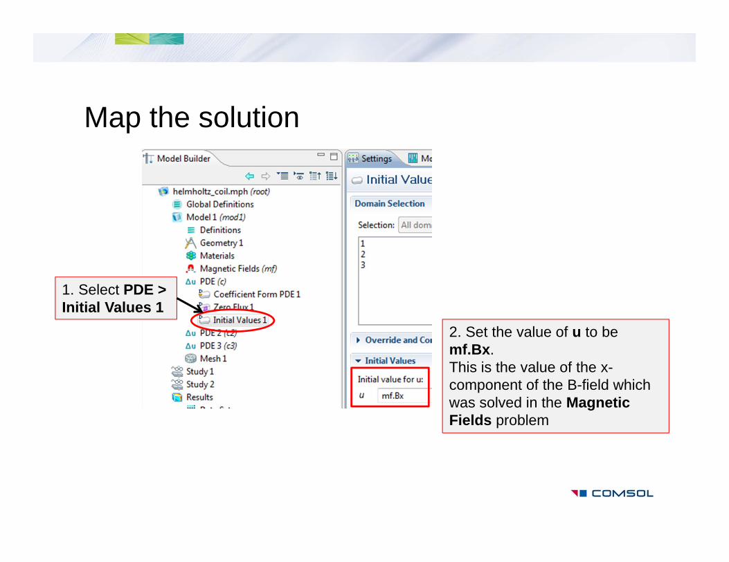
Map the solution

1. Select PDE > Initial Values 1

2. Set the value of u to be mf.Bx.This is the value of the x-component of the B-field which was solved in the Magnetic Fields problem

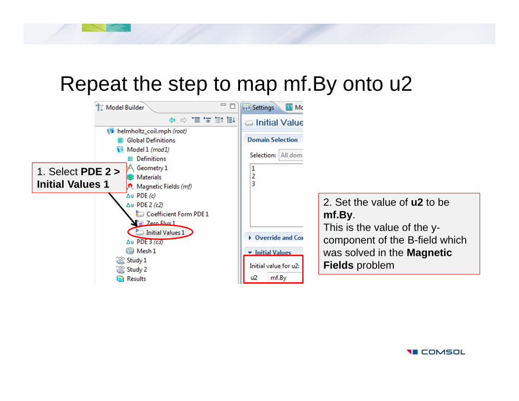
Repeat the step to map mf.By onto u2

1. Select PDE 2 > Initial Values 1

2. Set the value of u2 to be mf.By.This is the value of the y-component of the B-field which was solved in the Magnetic Fields problem

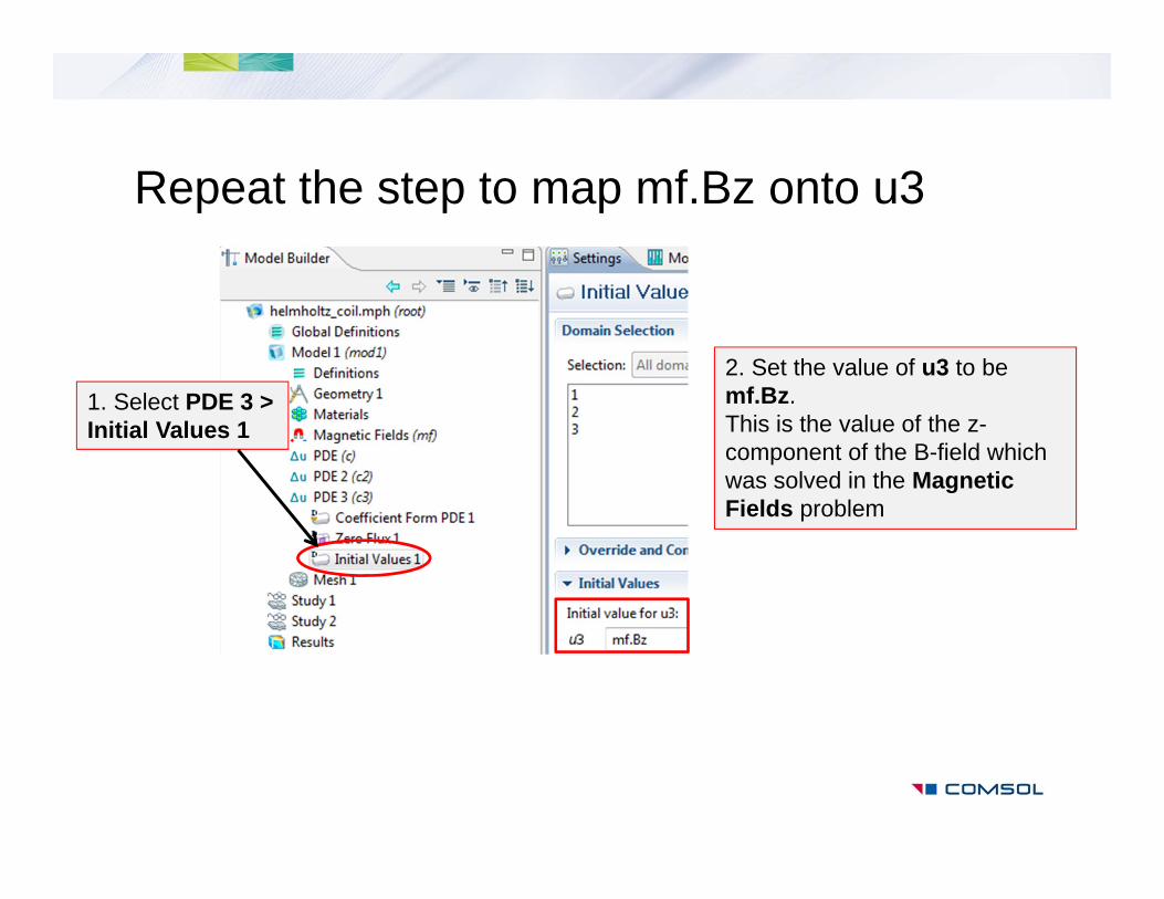
Repeat the step to map mf.Bz onto u3

1. Select PDE 3 > Initial Values 1

2. Set the value of u3 to be mf.Bz.This is the value of the z-component of the B-field which was solved in the Magnetic Fields problem

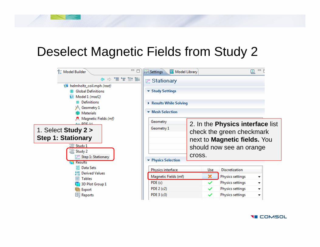
Deselect Magnetic Fields from Study 2

1. Select Study 2 > Step 1: Stationary

2. In the Physics interface list check the green checkmark next to Magnetic fields. You should now see an orange cross.

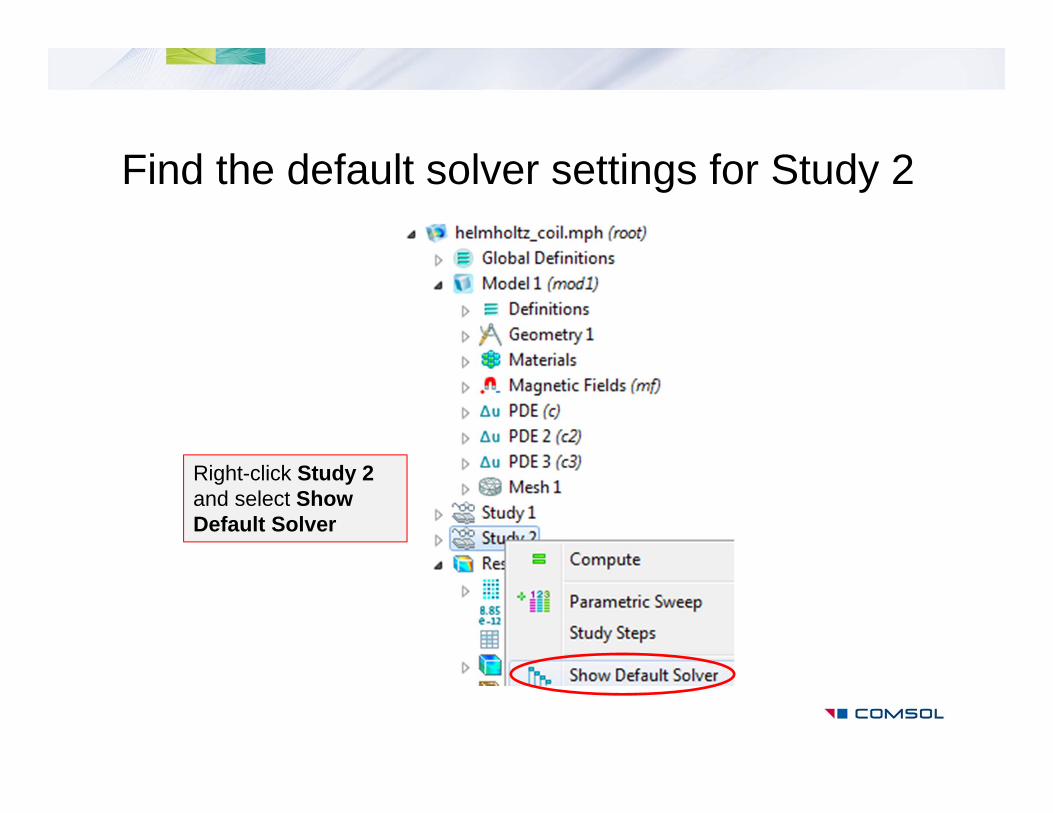
Find the default solver settings for Study 2

Right-click Study 2and select Show Default Solver

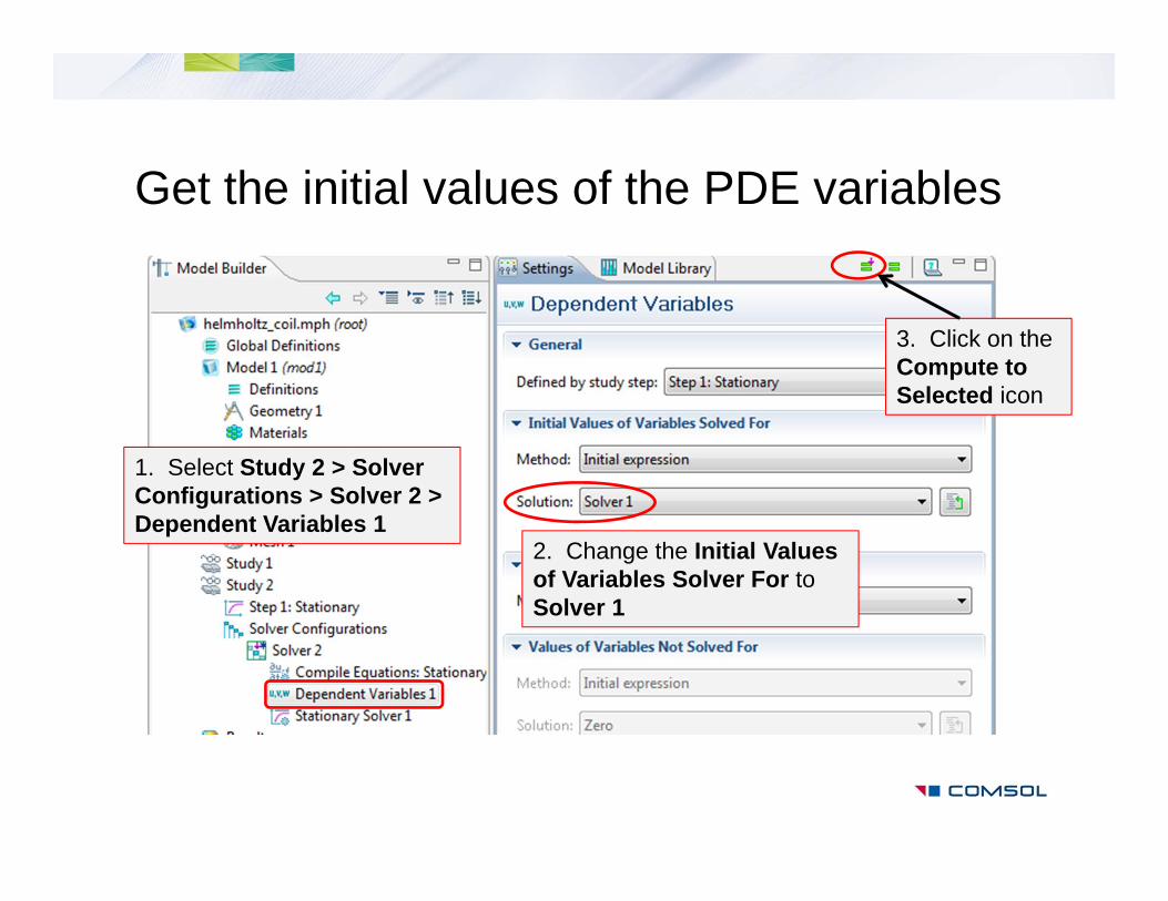
Get the initial values of the PDE variables

1. Select Study 2 > Solver Configurations > Solver 2 > Dependent Variables 1

2. Change the Initial Values of Variables Solver For to Solver 1

3. Click on the Compute to Selected icon

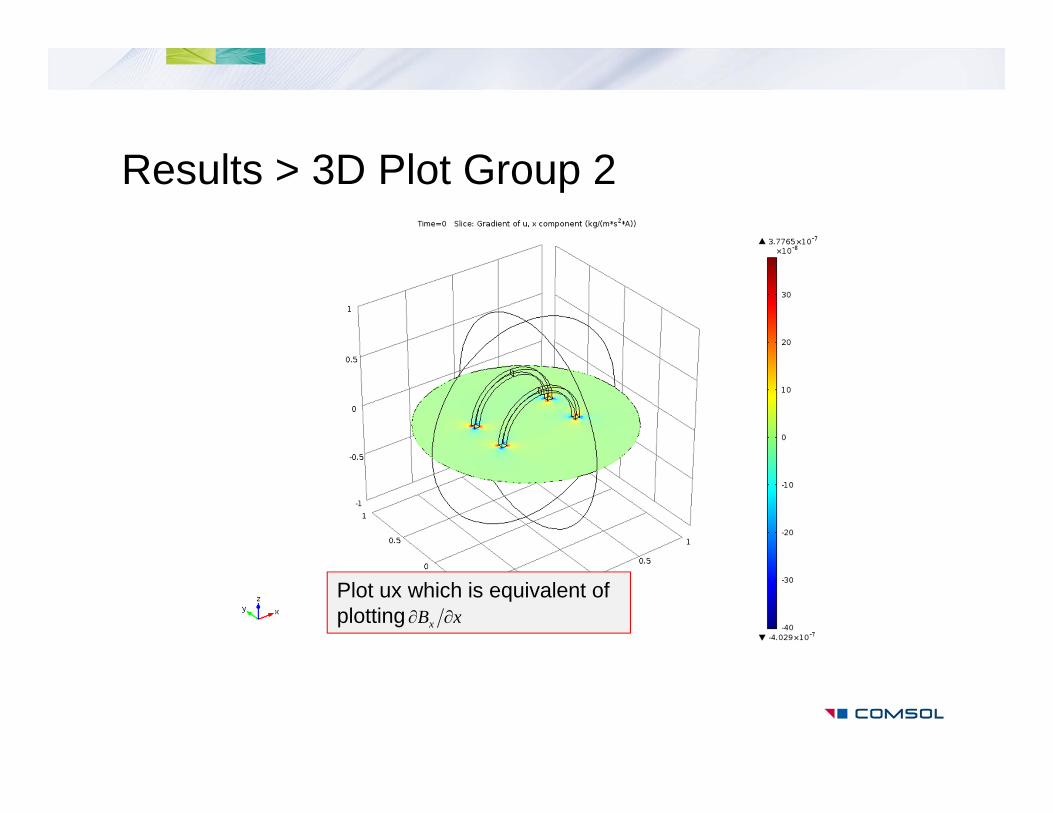
Results > 3D Plot Group 2

Plot ux which is equivalent of plotting xBx

Note on polynomial patch recovery (ppr)

• The polynomial patch recovery feature allows you to obtain smoother derivatives.

• How to use this feature?– You can either use the ppr or pprint functionOR…– Expand the Quality section of the plot settings

and see the Recover list

• Refer to the COMSOL MultiphysicsUser’s Guide for details.

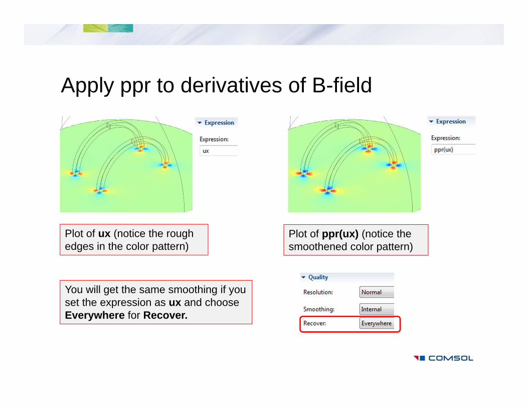
Apply ppr to derivatives of B-field

Plot of ux (notice the rough edges in the color pattern)

Plot of ppr(ux) (notice the smoothened color pattern)

You will get the same smoothing if you set the expression as ux and choose Everywhere for Recover.

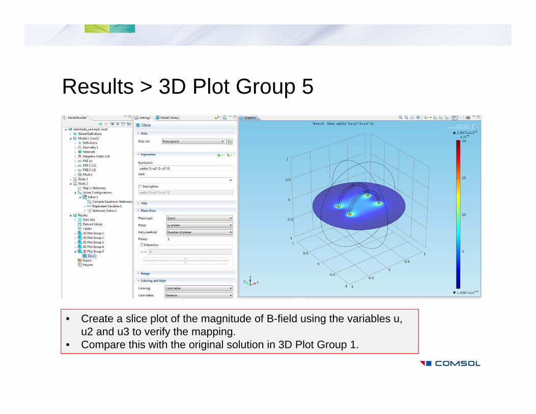
Results > 3D Plot Group 5

• Create a slice plot of the magnitude of B-field using the variables u, u2 and u3 to verify the mapping.

• Compare this with the original solution in 3D Plot Group 1.

Summary

• This tutorial showed how to visualize the spatial gradient of magnetic field.

• The magnetic field solution was mapped from vector elements to Lagrange elements.

• The derivative operations could be performed on the solution on the Lagrange elements.

• Mapping the solution onto Lagrange elements also give us the advantage to get smooth derivatives by using the polynomial patch recovery feature.