Gradient Estimation UsingStochastic Computation Graphs

John Schulman1,2

joschu@eecs.berkeley.eduNicolas Heess1

heess@google.com

Theophane Weber1

theophane@google.comPieter Abbeel2

pabbeel@eecs.berkeley.edu

1 Google DeepMind 2 University of California, Berkeley, EECS Department

AbstractIn a variety of problems originating in supervised, unsupervised, and reinforce-ment learning, the loss function is defined by an expectation over a collectionof random variables, which might be part of a probabilistic model or the exter-nal world. Estimating the gradient of this loss function, using samples, lies atthe core of gradient-based learning algorithms for these problems. We introducethe formalism of stochastic computation graphs—directed acyclic graphs that in-clude both deterministic functions and conditional probability distributions—anddescribe how to easily and automatically derive an unbiased estimator of the lossfunction’s gradient. The resulting algorithm for computing the gradient estimatoris a simple modification of the standard backpropagation algorithm. The genericscheme we propose unifies estimators derived in variety of prior work, along withvariance-reduction techniques therein. It could assist researchers in developing in-tricate models involving a combination of stochastic and deterministic operations,enabling, for example, attention, memory, and control actions.

1 IntroductionThe great success of neural networks is due in part to the simplicity of the backpropagation al-gorithm, which allows one to efficiently compute the gradient of any loss function defined as acomposition of differentiable functions. This simplicity has allowed researchers to search in thespace of architectures for those that are both highly expressive and conducive to optimization; yield-ing, for example, convolutional neural networks in vision [12] and LSTMs for sequence data [9].However, the backpropagation algorithm is only sufficient when the loss function is a deterministic,differentiable function of the parameter vector.

A rich class of problems arising throughout machine learning requires optimizing loss functionsthat involve an expectation over random variables. Two broad categories of these problems are (1)likelihood maximization in probabilistic models with latent variables [17, 18], and (2) policy gradi-ents in reinforcement learning [5, 23, 26]. Combining ideas from from those two perennial topics,recent models of attention [15] and memory [29] have used networks that involve a combination ofstochastic and deterministic operations.

In most of these problems, from probabilistic modeling to reinforcement learning, the loss functionsand their gradients are intractable, as they involve either a sum over an exponential number of latentvariable configurations, or high-dimensional integrals that have no analytic solution. Prior work (seeSection 6) has provided problem-specific derivations of Monte-Carlo gradient estimators, however,to our knowledge, no previous work addresses the general case.

Appendix C recalls several classic and recent techniques in variational inference [14, 10, 21] and re-inforcement learning [23, 25, 15], where the loss functions can be straightforwardly described using

1

arX

iv:1

506.

0525

4v3

[cs

.LG

] 5

Jan

201

6

the formalism of stochastic computation graphs that we introduce. For these examples, the variance-reduced gradient estimators derived in prior work are special cases of the results in Sections 3 and 4.

The contributions of this work are as follows:

• We introduce a formalism of stochastic computation graphs, and in this general setting, we deriveunbiased estimators for the gradient of the expected loss.

• We show how this estimator can be computed as the gradient of a certain differentiable function(which we call the surrogate loss), hence, it can be computed efficiently using the backpropaga-tion algorithm. This observation enables a practitioner to write an efficient implementation usingautomatic differentiation software.

• We describe variance reduction techniques that can be applied to the setting of stochastic compu-tation graphs, generalizing prior work from reinforcement learning and variational inference.

• We briefly describe how to generalize some other optimization techniques to this setting:majorization-minimization algorithms, by constructing an expression that bounds the loss func-tion; and quasi-Newton / Hessian-free methods [13], by computing estimates of Hessian-vectorproducts.

The main practical result of this article is that to compute the gradient estimator, one just needsto make a simple modification to the backpropagation algorithm, where extra gradient signals areintroduced at the stochastic nodes. Equivalently, the resulting algorithm is just the backpropagationalgorithm, applied to the surrogate loss function, which has extra terms introduced at the stochasticnodes. The modified backpropagation algorithm is presented in Section 5.

2 Preliminaries2.1 Gradient Estimators for a Single Random Variable

This section will discuss computing the gradient of an expectation taken over a single randomvariable—the estimators described here will be the building blocks for more complex cases withmultiple variables. Suppose that x is a random variable, f is a function (say, the cost), and we areinterested in computing ∂

∂θEx [f(x)]. There are a few different ways that the process for generatingx could be parameterized in terms of θ, which lead to different gradient estimators.

• We might be given a parameterized probability distribution x ∼ p(·; θ). In this case, we can usethe score function (SF) estimator [3]:

∂

∂θEx [f(x)] = Ex

[f(x)

∂

∂θlog p(x; θ)

]. (1)

This classic equation is derived as follows:∂

∂θEx [f(x)] =

∂

∂θ

∫dx p(x; θ)f(x) =

∫dx

∂

∂θp(x; θ)f(x)

=

∫dx p(x; θ)

∂

∂θlog p(x; θ)f(x) = Ex

[f(x)

∂

∂θlog p(x; θ)

]. (2)

This equation is valid if and only if p(x; θ) is a continuous function of θ; however, it does notneed to be a continuous function of x [4].

• x may be a deterministic, differentiable function of θ and another random variable z, i.e., we canwrite x(z, θ). Then, we can use the pathwise derivative (PD) estimator, defined as follows.

∂

∂θEz [f(x(z, θ))] = Ez

[∂

∂θf(x(z, θ))

]. (3)

This equation, which merely swaps the derivative and expectation, is valid if and only if f(x(z, θ))is a continuous function of θ for all z [4]. 1 That is not true if, for example, f is a step function.1 Note that for the pathwise derivative estimator, f(x(z, θ)) merely needs to be a continuous function of

θ—it is sufficient that this function is almost-everywhere differentiable. A similar statement can be madeabout p(x; θ) and the score function estimator. See Glasserman [4] for a detailed discussion of the technicalrequirements for these gradient estimators to be valid.

2

• Finally θ might appear both in the probability distribution and inside the expectation, e.g., in∂∂θEz∼p(·; θ) [f(x(z, θ))]. Then the gradient estimator has two terms:

∂

∂θEz∼p(·; θ) [f(x(z, θ))] = Ez∼p(·; θ)

[∂

∂θf(x(z, θ)) +

(∂

∂θlog p(z; θ)

)f(x(z, θ))

]. (4)

This formula can be derived by writing the expectation as an integral and differentiating, as inEquation (2).

In some cases, it is possible to reparameterize a probabilistic model—moving θ from the distributionto inside the expectation or vice versa. See [3] for a general discussion, and see [10, 21] for a recentapplication of this idea to variational inference.

The SF and PD estimators are applicable in different scenarios and have different properties.

1. SF is valid under more permissive mathematical conditions than PD. SF can be used if f isdiscontinuous, or if x is a discrete random variable.

2. SF only requires sample values f(x), whereas PD requires the derivatives f ′(x). In the contextof control (reinforcement learning), SF can be used to obtain unbiased policy gradient estimatorsin the “model-free” setting where we have no model of the dynamics, we only have access tosample trajectories.

3. SF tends to have higher variance than PD, when both estimators are applicable (see for instance[3, 21]). The variance of SF increases (often linearly) with the dimensionality of the sampledvariables. Hence, PD is usually preferable when x is high-dimensional. On the other hand, PDhas high variance if the function f is rough, which occurs in many time-series problems due toan “exploding gradient problem” / “butterfly effect”.

4. PD allows for a deterministic limit, SF does not. This idea is exploited by the deterministic policygradient algorithm [22].

Nomenclature. The methods of estimating gradients of expectations have been independently pro-posed in several different fields, which use differing terminology. What we call the score functionestimator (via [3]) is alternatively called the likelihood ratio estimator [5] and REINFORCE [26].We chose this term because the score function is a well-known object in statistics. What we callthe pathwise derivative estimator (from the mathematical finance literature [4] and reinforcementlearning [16]) is alternatively called infinitesimal perturbation analysis and stochastic backpropa-gation [21]. We chose this term because pathwise derivative is evocative of propagating a derivativethrough a sample path.

2.2 Stochastic Computation Graphs

The results of this article will apply to stochastic computation graphs, which are defined as follows:

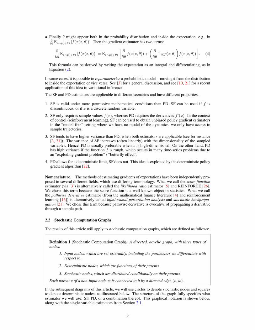
Definition 1 (Stochastic Computation Graph). A directed, acyclic graph, with three types ofnodes:

1. Input nodes, which are set externally, including the parameters we differentiate withrespect to.

2. Deterministic nodes, which are functions of their parents.

3. Stochastic nodes, which are distributed conditionally on their parents.

Each parent v of a non-input node w is connected to it by a directed edge (v, w).

In the subsequent diagrams of this article, we will use circles to denote stochastic nodes and squaresto denote deterministic nodes, as illustrated below. The structure of the graph fully specifies whatestimator we will use: SF, PD, or a combination thereof. This graphical notation is shown below,along with the single-variable estimators from Section 2.1.

3

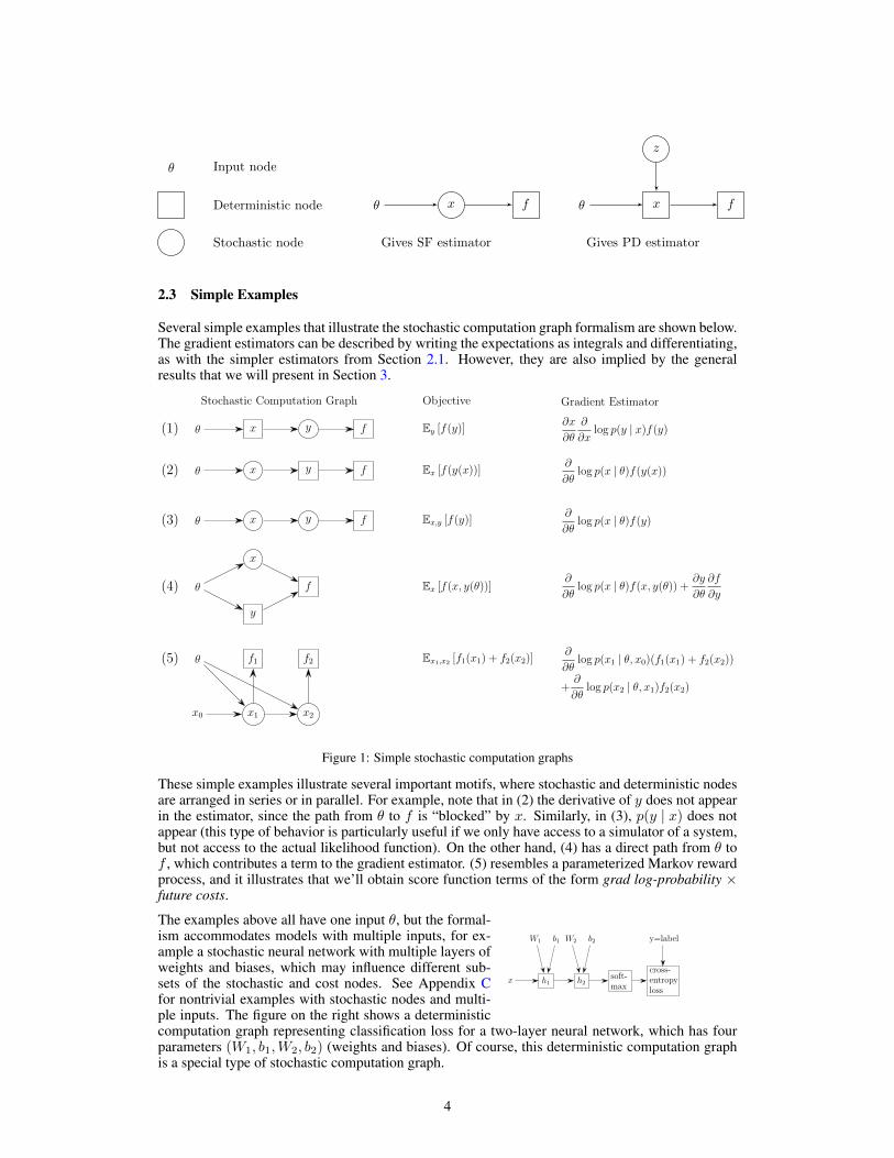
θ Input node

Deterministic node

Stochastic node

θ x f

Gives SF estimator

θ

z

x f

Gives PD estimator

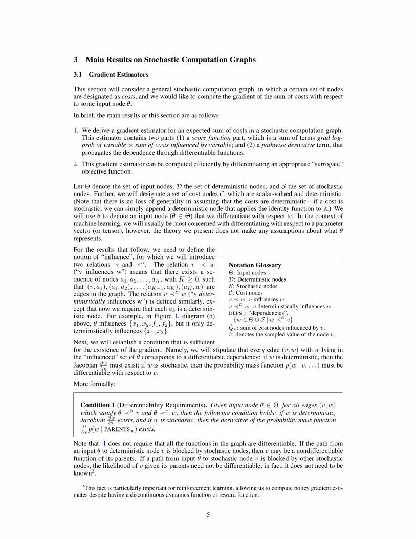
2.3 Simple Examples

Several simple examples that illustrate the stochastic computation graph formalism are shown below.The gradient estimators can be described by writing the expectations as integrals and differentiating,as with the simpler estimators from Section 2.1. However, they are also implied by the generalresults that we will present in Section 3.

Stochastic Computation Graph Objective Gradient Estimator

(1) θ x y f

(2) θ x y f

(3) θ x y f

(4) θ

x

y

f

(5) θ

x0 x1 x2

f1 f2

∂x

∂θ

∂

∂xlog p(y | x)f(y)

∂

∂θlog p(x | θ)f(y(x))

∂

∂θlog p(x | θ)f(y)

∂

∂θlog p(x | θ)f(x, y(θ)) + ∂y

∂θ

∂f

∂y

∂

∂θlog p(x1 | θ, x0)(f1(x1) + f2(x2))

+∂

∂θlog p(x2 | θ, x1)f2(x2)

Ey [f(y)]

Ex [f(y(x))]

Ex,y [f(y)]

Ex [f(x, y(θ))]

Ex1,x2 [f1(x1) + f2(x2)]

Figure 1: Simple stochastic computation graphs

These simple examples illustrate several important motifs, where stochastic and deterministic nodesare arranged in series or in parallel. For example, note that in (2) the derivative of y does not appearin the estimator, since the path from θ to f is “blocked” by x. Similarly, in (3), p(y | x) does notappear (this type of behavior is particularly useful if we only have access to a simulator of a system,but not access to the actual likelihood function). On the other hand, (4) has a direct path from θ tof , which contributes a term to the gradient estimator. (5) resembles a parameterized Markov rewardprocess, and it illustrates that we’ll obtain score function terms of the form grad log-probability ×future costs.

x h1 h2

W1 W2b1 b2

soft-max

y=label

cross-entropyloss

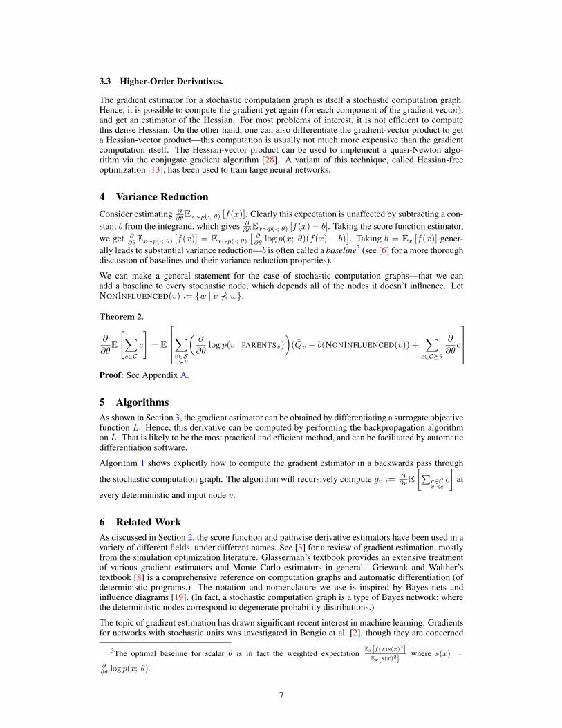
The examples above all have one input θ, but the formal-ism accommodates models with multiple inputs, for ex-ample a stochastic neural network with multiple layers ofweights and biases, which may influence different sub-sets of the stochastic and cost nodes. See Appendix Cfor nontrivial examples with stochastic nodes and multi-ple inputs. The figure on the right shows a deterministiccomputation graph representing classification loss for a two-layer neural network, which has fourparameters (W1, b1,W2, b2) (weights and biases). Of course, this deterministic computation graphis a special type of stochastic computation graph.

4

3 Main Results on Stochastic Computation Graphs

3.1 Gradient Estimators

This section will consider a general stochastic computation graph, in which a certain set of nodesare designated as costs, and we would like to compute the gradient of the sum of costs with respectto some input node θ.

In brief, the main results of this section are as follows:

1. We derive a gradient estimator for an expected sum of costs in a stochastic computation graph.This estimator contains two parts (1) a score function part, which is a sum of terms grad log-prob of variable × sum of costs influenced by variable; and (2) a pathwise derivative term, thatpropagates the dependence through differentiable functions.

2. This gradient estimator can be computed efficiently by differentiating an appropriate “surrogate”objective function.

Let Θ denote the set of input nodes, D the set of deterministic nodes, and S the set of stochasticnodes. Further, we will designate a set of cost nodes C, which are scalar-valued and deterministic.(Note that there is no loss of generality in assuming that the costs are deterministic—if a cost isstochastic, we can simply append a deterministic node that applies the identity function to it.) Wewill use θ to denote an input node (θ ∈ Θ) that we differentiate with respect to. In the context ofmachine learning, we will usually be most concerned with differentiating with respect to a parametervector (or tensor), however, the theory we present does not make any assumptions about what θrepresents.

Notation GlossaryΘ: Input nodesD: Deterministic nodesS: Stochastic nodesC: Cost nodesv ≺ w: v influences wv ≺D w: v deterministically influences wDEPSv: “dependencies”,{w ∈ Θ ∪ S | w ≺D v}

Qv: sum of cost nodes influenced by v.v: denotes the sampled value of the node v.

For the results that follow, we need to define thenotion of “influence”, for which we will introducetwo relations ≺ and ≺D. The relation v ≺ w(“v influences w”) means that there exists a se-quence of nodes a1, a2, . . . , aK , with K ≥ 0, suchthat (v, a1), (a1, a2), . . . , (aK−1, aK), (aK , w) areedges in the graph. The relation v ≺D w (“v deter-ministically influences w”) is defined similarly, ex-cept that now we require that each ak is a determin-istic node. For example, in Figure 1, diagram (5)above, θ influences {x1, x2, f1, f2}, but it only de-terministically influences {x1, x2}.Next, we will establish a condition that is sufficientfor the existence of the gradient. Namely, we will stipulate that every edge (v, w) with w lying inthe “influenced” set of θ corresponds to a differentiable dependency: if w is deterministic, then theJacobian ∂w

∂v must exist; if w is stochastic, then the probability mass function p(w | v, . . . ) must bedifferentiable with respect to v.

More formally:

Condition 1 (Differentiability Requirements). Given input node θ ∈ Θ, for all edges (v, w)which satisfy θ ≺D v and θ ≺D w, then the following condition holds: if w is deterministic,Jacobian ∂w

∂v exists, and if w is stochastic, then the derivative of the probability mass function∂∂vp(w | PARENTSw) exists.

Note that 1 does not require that all the functions in the graph are differentiable. If the path froman input θ to deterministic node v is blocked by stochastic nodes, then v may be a nondifferentiablefunction of its parents. If a path from input θ to stochastic node v is blocked by other stochasticnodes, the likelihood of v given its parents need not be differentiable; in fact, it does not need to beknown2.

2This fact is particularly important for reinforcement learning, allowing us to compute policy gradient esti-mates despite having a discontinuous dynamics function or reward function.

5

We need a few more definitions to state the main theorems. Let DEPSv := {w ∈ Θ ∪ S | w ≺D v},the “dependencies” of node v, i.e., the set of nodes that deterministically influence it. Note thefollowing:

• If v ∈ S, the probability mass function of v is a function of DEPSv , i.e., we can write p(v |DEPSv).• If v ∈ D, v is a deterministic function of DEPSv , so we can write v(DEPSv).

Let Qv :=∑c�v,c∈C

c, i.e., the sum of costs downstream of node v. These costs will be treated as

constant, fixed to the values obtained during sampling. In general, we will use the hat symbol v todenote a sample value of variable v, which will be treated as constant in the gradient formulae.

Now we can write down a general expression for the gradient of the expected sum of costs in astochastic computation graph:

Theorem 1. Suppose that θ ∈ Θ satisfies 1. Then the following two equivalent equations hold:

∂

∂θE

[∑c∈C

c

]= E

∑w∈S,θ≺Dw

(∂

∂θlog p(w | DEPSw)

)Qw +

∑c∈Cθ≺Dc

∂

∂θc(DEPSc)

(5)

= E

∑c∈C

c∑w≺c,θ≺Dw

∂

∂θlog p(w | DEPSw) +

∑c∈C,θ≺Dc

∂

∂θc(DEPSc)

. (6)

Proof: See Appendix A.

The estimator expressions above have two terms. The first term is due to the influence of θ on proba-bility distributions. The second term is due to the influence of θ on the cost variables through a chainof differentiable functions. The distribution term involves a sum of gradients times “downstream”costs. The first term in Equation (5) involves a sum of gradients times “downstream” costs, whereasthe first term in Equation (6) has a sum of costs times “upstream” gradients.

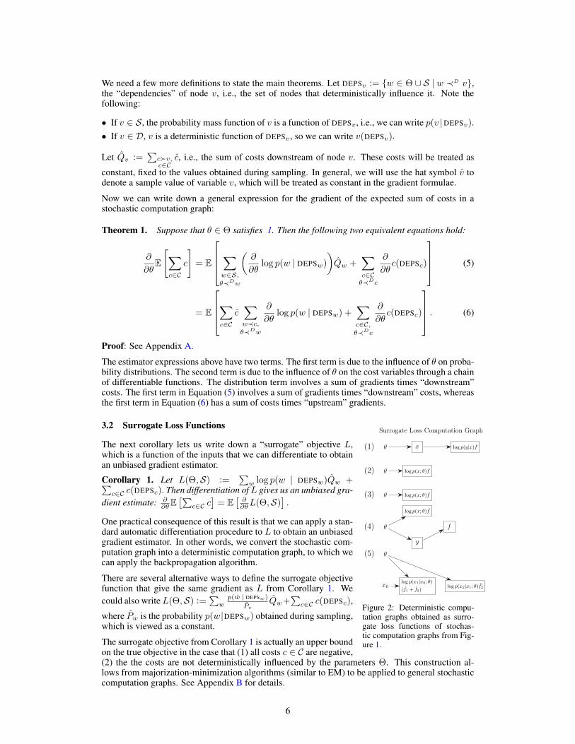
3.2 Surrogate Loss FunctionsSurrogate Loss Computation Graph

(1) θ x log p(y|x)f

(2) θ log p(x; θ)f

(3) θ log p(x; θ)f

(4) θ

log p(x; θ)f

y

f

(5) θ

x0log p(x1|x0; θ)(f1 + f2)

log p(x2|x1; θ)f2

Figure 2: Deterministic compu-tation graphs obtained as surro-gate loss functions of stochas-tic computation graphs from Fig-ure 1.

The next corollary lets us write down a “surrogate” objective L,which is a function of the inputs that we can differentiate to obtainan unbiased gradient estimator.

Corollary 1. Let L(Θ,S) :=∑w log p(w | DEPSw)Qw +∑

c∈C c(DEPSc). Then differentiation ofL gives us an unbiased gra-dient estimate: ∂

∂θE[∑

c∈C c]

= E[∂∂θL(Θ,S)

].

One practical consequence of this result is that we can apply a stan-dard automatic differentiation procedure to L to obtain an unbiasedgradient estimator. In other words, we convert the stochastic com-putation graph into a deterministic computation graph, to which wecan apply the backpropagation algorithm.

There are several alternative ways to define the surrogate objectivefunction that give the same gradient as L from Corollary 1. Wecould also writeL(Θ,S) :=

∑wp(w | DEPSw)

PvQw+

∑c∈C c(DEPSc),

where Pw is the probability p(w|DEPSw) obtained during sampling,which is viewed as a constant.

The surrogate objective from Corollary 1 is actually an upper boundon the true objective in the case that (1) all costs c ∈ C are negative,(2) the the costs are not deterministically influenced by the parameters Θ. This construction al-lows from majorization-minimization algorithms (similar to EM) to be applied to general stochasticcomputation graphs. See Appendix B for details.

6

3.3 Higher-Order Derivatives.

The gradient estimator for a stochastic computation graph is itself a stochastic computation graph.Hence, it is possible to compute the gradient yet again (for each component of the gradient vector),and get an estimator of the Hessian. For most problems of interest, it is not efficient to computethis dense Hessian. On the other hand, one can also differentiate the gradient-vector product to geta Hessian-vector product—this computation is usually not much more expensive than the gradientcomputation itself. The Hessian-vector product can be used to implement a quasi-Newton algo-rithm via the conjugate gradient algorithm [28]. A variant of this technique, called Hessian-freeoptimization [13], has been used to train large neural networks.

4 Variance ReductionConsider estimating ∂

∂θEx∼p(·; θ) [f(x)]. Clearly this expectation is unaffected by subtracting a con-stant b from the integrand, which gives ∂

∂θEx∼p(·; θ) [f(x)− b]. Taking the score function estimator,we get ∂

∂θEx∼p(·; θ) [f(x)] = Ex∼p(·; θ)[∂∂θ log p(x; θ)(f(x)− b)

]. Taking b = Ex [f(x)] gener-

ally leads to substantial variance reduction—b is often called a baseline3 (see [6] for a more thoroughdiscussion of baselines and their variance reduction properties).

We can make a general statement for the case of stochastic computation graphs—that we canadd a baseline to every stochastic node, which depends all of the nodes it doesn’t influence. LetNONINFLUENCED(v) := {w | v ⊀ w}.

Theorem 2.

∂

∂θE

[∑c∈C

c

]= E

∑v∈Sv�θ

(∂

∂θlog p(v | PARENTSv)

)(Qv − b(NONINFLUENCED(v)) +

∑c∈C�θ

∂

∂θc

Proof: See Appendix A.

5 AlgorithmsAs shown in Section 3, the gradient estimator can be obtained by differentiating a surrogate objectivefunction L. Hence, this derivative can be computed by performing the backpropagation algorithmon L. That is likely to be the most practical and efficient method, and can be facilitated by automaticdifferentiation software.

Algorithm 1 shows explicitly how to compute the gradient estimator in a backwards pass through

the stochastic computation graph. The algorithm will recursively compute gv := ∂∂vE

[∑c∈Cv≺c

c

]at

every deterministic and input node v.

6 Related WorkAs discussed in Section 2, the score function and pathwise derivative estimators have been used in avariety of different fields, under different names. See [3] for a review of gradient estimation, mostlyfrom the simulation optimization literature. Glasserman’s textbook provides an extensive treatmentof various gradient estimators and Monte Carlo estimators in general. Griewank and Walther’stextbook [8] is a comprehensive reference on computation graphs and automatic differentiation (ofdeterministic programs.) The notation and nomenclature we use is inspired by Bayes nets andinfluence diagrams [19]. (In fact, a stochastic computation graph is a type of Bayes network; wherethe deterministic nodes correspond to degenerate probability distributions.)

The topic of gradient estimation has drawn significant recent interest in machine learning. Gradientsfor networks with stochastic units was investigated in Bengio et al. [2], though they are concerned

3The optimal baseline for scalar θ is in fact the weighted expectationEx[f(x)s(x)2]

Ex[s(x)2]where s(x) =

∂∂θ

log p(x; θ).

7

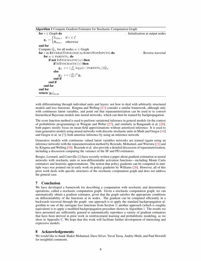
Algorithm 1 Compute Gradient Estimator for Stochastic Computation Graphfor v ∈ Graph do . Initialization at output nodes

gv =

{1dim v if v ∈ C0dim v otherwise

end forCompute Qw for all nodes w ∈ Graphfor v in REVERSETOPOLOGICALSORT(NONINPUTS) do . Reverse traversal

for w ∈ PARENTSv doif not ISSTOCHASTIC(w) then

if ISSTOCHASTIC(v) thengw += ( ∂

∂w log p(v | PARENTSv))Qwelse

gw += ( ∂v∂w )Tgvend if

end ifend for

end forreturn [gθ]θ∈Θ

with differentiating through individual units and layers; not how to deal with arbitrarily structuredmodels and loss functions. Kingma and Welling [11] consider a similar framework, although onlywith continuous latent variables, and point out that reparameterization can be used to to converthierarchical Bayesian models into neural networks, which can then be trained by backpropagation.

The score function method is used to perform variational inference in general models (in the contextof probabilistic programming) in Wingate and Weber [27], and similarly in Ranganath et al. [20];both papers mostly focus on mean-field approximations without amortized inference. It is used totrain generative models using neural networks with discrete stochastic units in Mnih and Gregor [14]and Gregor et al. in [7]; both amortize inference by using an inference network.

Generative models with continuous valued latent variables networks are trained (again using aninference network) with the reparametrization method by Rezende, Mohamed, and Wierstra [21] andby Kingma and Welling [10]. Rezende et al. also provide a detailed discussion of reparameterization,including a discussion comparing the variance of the SF and PD estimators.

Bengio, Leonard, and Courville [2] have recently written a paper about gradient estimation in neuralnetworks with stochastic units or non-differentiable activation functions—including Monte Carloestimators and heuristic approximations. The notion that policy gradients can be computed in mul-tiple ways was pointed out in early work on policy gradients by Williams [26]. However, all of thisprior work deals with specific structures of the stochastic computation graph and does not addressthe general case.

7 ConclusionWe have developed a framework for describing a computation with stochastic and deterministicoperations, called a stochastic computation graph. Given a stochastic computation graph, we canautomatically obtain a gradient estimator, given that the graph satisfies the appropriate conditionson differentiability of the functions at its nodes. The gradient can be computed efficiently in abackwards traversal through the graph: one approach is to apply the standard backpropagation al-gorithm to one of the surrogate loss functions from Section 3; another approach (which is roughlyequivalent) is to apply a modified backpropagation procedure shown in Algorithm 1. The results wehave presented are sufficiently general to automatically reproduce a variety of gradient estimatorsthat have been derived in prior work in reinforcement learning and probabilistic modeling, as weshow in Appendix C. We hope that this work will facilitate further development of interesting andexpressive models.

8 AcknowledgementsWe would like to thank Shakir Mohamed, Dave Silver, Yuval Tassa, Andriy Mnih, and Paul Horsfallfor insightful comments.

8

References[1] J. Baxter and P. L. Bartlett. Infinite-horizon policy-gradient estimation. Journal of Artificial Intelligence

Research, pages 319–350, 2001.[2] Y. Bengio, N. Leonard, and A. Courville. Estimating or propagating gradients through stochastic neurons

for conditional computation. arXiv preprint arXiv:1308.3432, 2013.[3] M. C. Fu. Gradient estimation. Handbooks in operations research and management science, 13:575–616,

2006.[4] P. Glasserman. Monte Carlo methods in financial engineering, volume 53. Springer Science & Business

Media, 2003.[5] P. W. Glynn. Likelihood ratio gradient estimation for stochastic systems. Communications of the ACM,

33(10):75–84, 1990.[6] E. Greensmith, P. L. Bartlett, and J. Baxter. Variance reduction techniques for gradient estimates in

reinforcement learning. The Journal of Machine Learning Research, 5:1471–1530, 2004.[7] K. Gregor, I. Danihelka, A. Mnih, C. Blundell, and D. Wierstra. Deep autoregressive networks. arXiv

preprint arXiv:1310.8499, 2013.[8] A. Griewank and A. Walther. Evaluating derivatives: principles and techniques of algorithmic differenti-

ation. Siam, 2008.[9] S. Hochreiter and J. Schmidhuber. Long short-term memory. Neural computation, 9(8):1735–1780, 1997.

[10] D. P. Kingma and M. Welling. Auto-encoding variational Bayes. arXiv:1312.6114, 2013.[11] D. P. Kingma and M. Welling. Efficient gradient-based inference through transformations between bayes

nets and neural nets. arXiv preprint arXiv:1402.0480, 2014.[12] Y. LeCun, L. Bottou, Y. Bengio, and P. Haffner. Gradient-based learning applied to document recognition.

Proceedings of the IEEE, 86(11):2278–2324, 1998.[13] J. Martens. Deep learning via Hessian-free optimization. In Proceedings of the 27th International Con-

ference on Machine Learning (ICML-10), pages 735–742, 2010.[14] A. Mnih and K. Gregor. Neural variational inference and learning in belief networks. arXiv:1402.0030,

2014.[15] V. Mnih, N. Heess, A. Graves, and K. Kavukcuoglu. Recurrent models of visual attention. In Advances

in Neural Information Processing Systems, pages 2204–2212, 2014.[16] R. Munos. Policy gradient in continuous time. The Journal of Machine Learning Research, 7:771–791,

2006.[17] R. M. Neal. Learning stochastic feedforward networks. Department of Computer Science, University of

Toronto, 1990.[18] R. M. Neal and G. E. Hinton. A view of the em algorithm that justifies incremental, sparse, and other

variants. In Learning in graphical models, pages 355–368. Springer, 1998.[19] J. Pearl. Probabilistic reasoning in intelligent systems: networks of plausible inference. Morgan Kauf-

mann, 2014.[20] R. Ranganath, S. Gerrish, and D. M. Blei. Black box variational inference. arXiv preprint

arXiv:1401.0118, 2013.[21] D. J. Rezende, S. Mohamed, and D. Wierstra. Stochastic backpropagation and approximate inference in

deep generative models. arXiv:1401.4082, 2014.[22] D. Silver, G. Lever, N. Heess, T. Degris, D. Wierstra, and M. Riedmiller. Deterministic policy gradient

algorithms. In ICML, 2014.[23] R. S. Sutton, D. A. McAllester, S. P. Singh, Y. Mansour, et al. Policy gradient methods for reinforcement

learning with function approximation. In NIPS, volume 99, pages 1057–1063. Citeseer, 1999.[24] N. Vlassis, M. Toussaint, G. Kontes, and S. Piperidis. Learning model-free robot control by a Monte

Carlo EM algorithm. Autonomous Robots, 27(2):123–130, 2009.[25] D. Wierstra, A. Forster, J. Peters, and J. Schmidhuber. Recurrent policy gradients. Logic Journal of IGPL,

18(5):620–634, 2010.[26] R. J. Williams. Simple statistical gradient-following algorithms for connectionist reinforcement learning.

Machine learning, 8(3-4):229–256, 1992.[27] D. Wingate and T. Weber. Automated variational inference in probabilistic programming. arXiv preprint

arXiv:1301.1299, 2013.[28] S. J. Wright and J. Nocedal. Numerical optimization, volume 2. Springer New York, 1999.[29] W. Zaremba and I. Sutskever. Reinforcement learning neural Turing machines. arXiv preprint

arXiv:1505.00521, 2015.

9

A ProofsTheorem 1

We will consider the case that all of the random variables are continuous-valued, thus the expecta-tions can be written as integrals. For discrete random variables, the integrals should be changed tosums.

Recall that we seek to compute ∂∂θE

[∑c∈C c

]. We will differentiate the expectation of a single cost

term; summing over these terms yields Equation (6).

Ev∈S,v≺c

[c] =

∫ ∏v∈S,v≺c

p(v | DEPSv)dv c(DEPSc) (7)

∂

∂θEv∈S,v≺c

[c] =∂

∂θ

∫ ∏v∈S,v≺c

p(v | DEPSv)dv c(DEPSc) (8)

=

∫ ∏v∈S,v≺c

p(v | DEPSv)dv

∑w∈S,w≺c

∂∂θp(w | DEPSw)

p(w | DEPSw)c(DEPSc) +

∂

∂θc(DEPSc)

(9)

=

∫ ∏v∈S,v≺c

p(v | DEPSv)dv

∑w∈S,w≺c

(∂

∂θlog p(w | DEPSw)

)c(DEPSc) +

∂

∂θc(DEPSc)

(10)

= Ev∈S,v≺c

∑w∈S,w≺c

∂

∂θlog p(w | DEPSw)c+

∂

∂θc(DEPSc)

. (11)

Equation (9) requires that the integrand is differentiable, which is satisfied if all of the PDFs andc(DEPSc) are differentiable. Equation (6) follows by summing over all costs c ∈ C. Equation (5)follows from rearrangement of the terms in this equation.

Theorem 2

It suffices to show that for a particular node v ∈ S, the following expectation (taken over all vari-ables) vanishes

E[(

∂

∂θlog p(v | PARENTSv)

)b(NONINFLUENCED(v))

]. (12)

Analogously to NONINFLUENCED(v), define INFLUENCED(v) := {w | w � v}. Note that thenodes can be ordered so that NONINFLUENCED(v) all come before v in the ordering. Thus, wecan write

ENONINFLUENCED(v)

[EINFLUENCED(v)

[(∂

∂θlog p(v | PARENTSv)

)b(NONINFLUENCED(v))

]](13)

= ENONINFLUENCED(v)

[EINFLUENCED(v)

[(∂

∂θlog p(v | PARENTSv)

)]b(NONINFLUENCED(v))

](14)

= ENONINFLUENCED(v) [0 · b(NONINFLUENCED(v))] (15)

= 0 (16)

where we used EINFLUENCED(v)

[(∂∂θ log p(v | PARENTSv)

)]= Ev

[(∂∂θ log p(v | PARENTSv)

)]= 0.

B Surrogate as an Upper Bound, and MM AlgorithmsL has additional significance besides allowing us to estimate the gradient of the expected sum ofcosts. Under certain conditions, L is a upper bound on on the true objective (plus a constant).

10

We shall make two restrictions on the stochastic computation graph: (1) first, that all costs c ∈ Care negative. (2) the the costs are not deterministically influenced by the parameters Θ. First, letus use importance sampling to write down the expectation of a given cost node, when the samplingdistribution is different from the distribution we are evaluating: for parameter θ ∈ Θ, θ = θold isused for sampling, but we are evaluating at θ = θnew.

Ev≺c | θnew[c] = Ev≺c | θold

c ∏v≺c,θ≺Dv

Pv(v | DEPSv\θ, θnew)

Pv(v | DEPSv\θ, θold)

(17)

≤ Ev≺c | θold

clog

∏v≺c,θ≺Dv

Pv(v | DEPSv\θ, θnew)

Pv(v | DEPSv\θ, θold)

+ 1

(18)

where the second line used the inequality x ≥ log x+ 1, and the sign is reversed since c is negative.Summing over c ∈ C and rearranging we get

ES | θnew

[∑c∈C

c

]≤ ES | θold

[∑c∈C

c+∑v∈S

log

(p(v | DEPSv\θ, θnew)

p(v | DEPSv\θ, θold)

)Qv

](19)

= ES | θold

[∑v∈S

log p(v | DEPSv\θ, θnew)Qv

]+ const. (20)

Equation (20) allows for majorization-minimization algorithms (like the EM algorithm) to be usedto optimize with respect to θ. In fact, similar equations have been derived by interpreting rewards(negative costs) as probabilities, and then taking the variational lower bound on log-probability (e.g.,[24]).

C ExamplesThis section considers two settings where the formalism of stochastic computation graphs can beapplied. First, we consider the generalized EM algorithm for maximum likelihood estimation inprobabilistic models with latent variables. Second, we consider reinforcement learning in MarkovDecision Processes. In both cases, the objective function is given by an expectation; writing it outas a composition of stochastic and deterministic steps yields a stochastic computation graph.

C.1 Generalized EM Algorithm and Variational Inference.

The generalized EM algorithm maximizes likelihood in a probabilistic model with latent variables[18]. We start with a parameterized probability density p(x, z; θ) where x is observed, z is a latentvariable, and θ is a parameter of the distribution. The generalized EM algorithm maximizes thevariational lower bound, which is defined by an expectation over z for each sample x:

L(θ, q) = Ez∼q[log

(p(x, z; θ)

q(z)

)]. (21)

As parameters will appear both in the probability density and inside the expectation, stochasticcomputation graphs provide a convenient route for deriving the gradient estimators.

x h1 h2 h3

r1 r2 r3

φ1 φ2 φ3

θ1 θ2 θ3

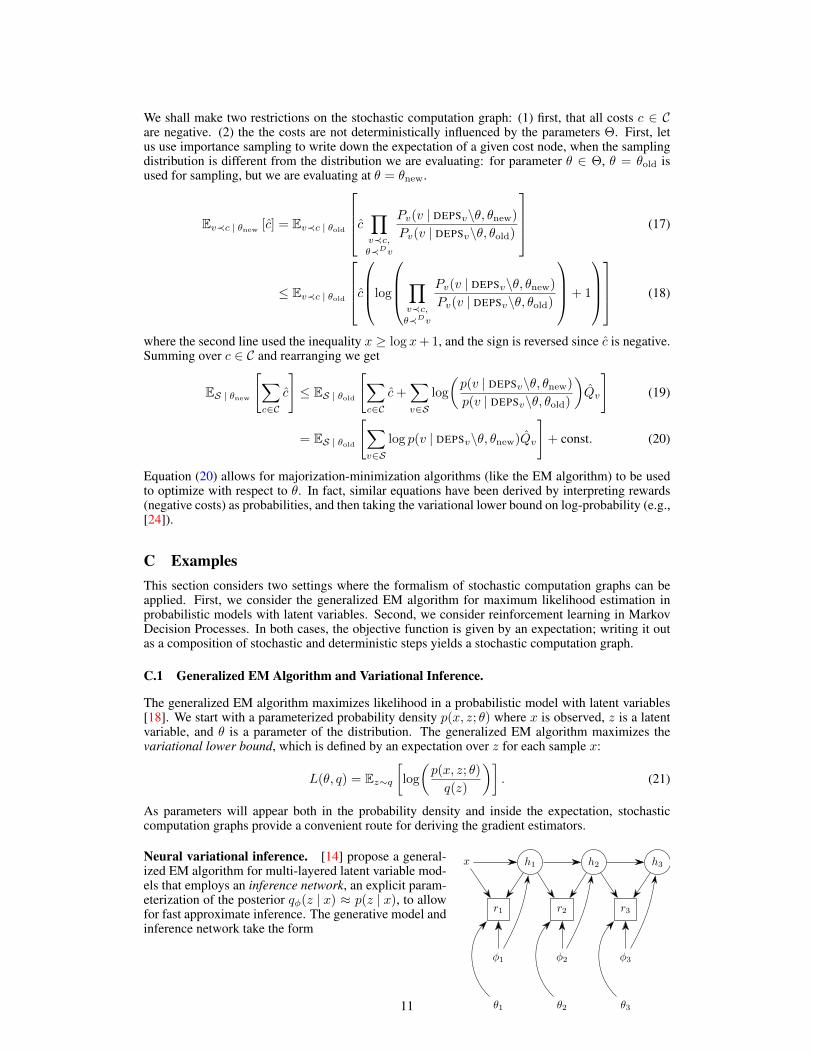
Neural variational inference. [14] propose a general-ized EM algorithm for multi-layered latent variable mod-els that employs an inference network, an explicit param-eterization of the posterior qφ(z | x) ≈ p(z | x), to allowfor fast approximate inference. The generative model andinference network take the form

11

pθ(x) =∑h1,h2

pθ1(x|h1)pθ2(h1|h2)pθ3(h2|h3)pθ3(h3)

qφ(h1, h2|x) = qφ1(h1|x)qφ2

(h2|h1)qφ3(h3|h2).

The inference model qφ is used for sampling, i.e., we sample h1 ∼ qφ1(· |x), h2 ∼ qφ2

(· |h1), h3 ∼qφ3

(· | h2). The stochastic computation graph is shown above.

L(θ, φ) = Eh∼qφ

logpθ1(x|h1)

qφ1(h1|x)︸ ︷︷ ︸=r1

+ logpθ2(h1|h2)

qφ2(h2|h1)︸ ︷︷ ︸=r2

+ logpθ3(h2|h3)pθ3(h3)

qφ3(h3|h2)︸ ︷︷ ︸=r3

.Given a sample h ∼ qφ an unbiased estimate of the gradient is given by Theorem 2 as

∂L

∂θ≈ ∂

∂θlog pθ1(x|h1) +

∂

∂θlog pθ2(h1|h2) +

∂

∂θlog pθ3(h2) (22)

∂L

∂φ≈ ∂

∂φlog qφ1(h1|x)(Q1 − b1(x))

+∂

∂φlog qφ2

(h2|h1)(Q2 − b2(h1)) +∂

∂φlog qφ3

(h3|h2)(Q3 − b3(h2)) (23)

where Q1 = r1 + r2 + r3; Q2 = r2 + r3; and Q3 = r3, and b1, b2, b3 are baseline functions.

x h1 z h2 x

L

φ θ

⇓ Reparameterization

x h1 z h2 x

L

φ θε

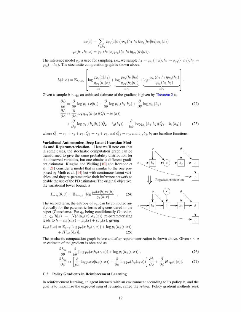
Variational Autoencoder, Deep Latent Gaussian Mod-els and Reparameterization. Here we’ll note out thatin some cases, the stochastic computation graph can betransformed to give the same probability distribution forthe observed variables, but one obtains a different gradi-ent estimator. Kingma and Welling [10] and Rezende etal. [21] consider a model that is similar to the one pro-posed by Mnih et al. [14] but with continuous latent vari-ables, and they re-parameterize their inference network toenable the use of the PD estimator. The original objective,the variational lower bound, is

Lorig(θ, φ) = Eh∼qφ[log

pθ(x|h)pθ(h)

qφ(h|x)

]. (24)

The second term, the entropy of qφ, can be computed an-alytically for the parametric forms of q considered in thepaper (Gaussians). For qφ being conditionally Gaussian,i.e. qφ(h|x) = N(h|µφ(x), σφ(x)) re-parameterizingleads to h = hφ(ε;x) = µφ(x) + εσφ(x), giving

Lre(θ, φ) = Eε∼ρ [log pθ(x|hφ(ε, x)) + log pθ(hφ(ε, x))]

+H[qφ(·|x)]. (25)

The stochastic computation graph before and after reparameterization is shown above. Given ε ∼ ρan estimate of the gradient is obtained as

∂Lre

∂θ≈ ∂

∂θ[log pθ(x|hφ(ε, x)) + log pθ(hφ(ε, x))] , (26)

∂Lre

∂φ≈[∂

∂hlog pθ(x|hφ(ε, x)) +

∂

∂hlog pθ(hφ(ε, x))

]∂h

∂φ+

∂

∂φH[qφ(·|x)]. (27)

C.2 Policy Gradients in Reinforcement Learning.

In reinforcement learning, an agent interacts with an environment according to its policy π, and thegoal is to maximize the expected sum of rewards, called the return. Policy gradient methods seek

12

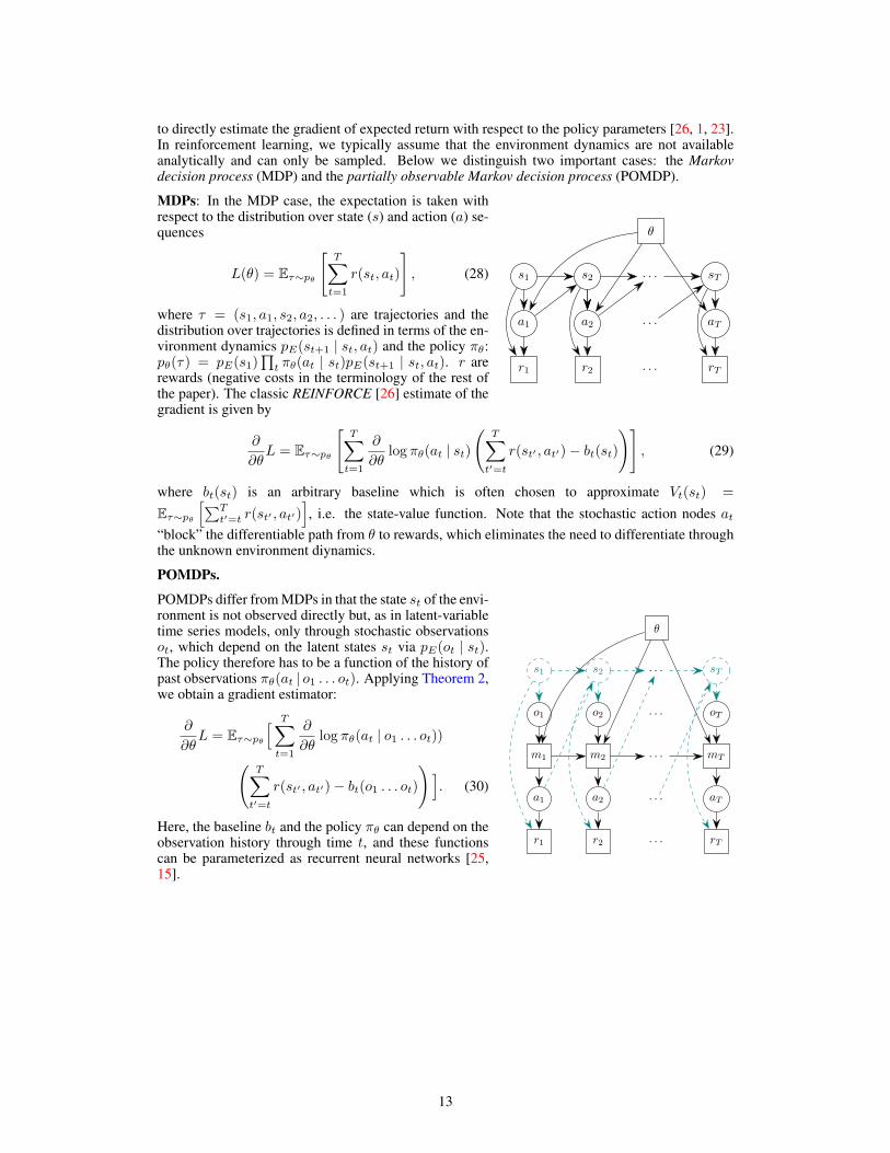
to directly estimate the gradient of expected return with respect to the policy parameters [26, 1, 23].In reinforcement learning, we typically assume that the environment dynamics are not availableanalytically and can only be sampled. Below we distinguish two important cases: the Markovdecision process (MDP) and the partially observable Markov decision process (POMDP).

θ

s1 s2 . . . sT

a1 a2 . . . aT

r1 r2 . . . rT

MDPs: In the MDP case, the expectation is taken withrespect to the distribution over state (s) and action (a) se-quences

L(θ) = Eτ∼pθ

[T∑t=1

r(st, at)

], (28)

where τ = (s1, a1, s2, a2, . . . ) are trajectories and thedistribution over trajectories is defined in terms of the en-vironment dynamics pE(st+1 | st, at) and the policy πθ:pθ(τ) = pE(s1)

∏t πθ(at | st)pE(st+1 | st, at). r are

rewards (negative costs in the terminology of the rest ofthe paper). The classic REINFORCE [26] estimate of thegradient is given by

∂

∂θL = Eτ∼pθ

[T∑t=1

∂

∂θlog πθ(at | st)

(T∑t′=t

r(st′ , at′)− bt(st))]

, (29)

where bt(st) is an arbitrary baseline which is often chosen to approximate Vt(st) =

Eτ∼pθ[∑T

t′=t r(st′ , at′)], i.e. the state-value function. Note that the stochastic action nodes at

“block” the differentiable path from θ to rewards, which eliminates the need to differentiate throughthe unknown environment diynamics.

POMDPs.

θ

s1 s2 . . . sT

o1 o2 . . . oT

m1 m2 . . . mT

a1 a2 . . . aT

r1 r2 . . . rT

POMDPs differ from MDPs in that the state st of the envi-ronment is not observed directly but, as in latent-variabletime series models, only through stochastic observationsot, which depend on the latent states st via pE(ot | st).The policy therefore has to be a function of the history ofpast observations πθ(at | o1 . . . ot). Applying Theorem 2,we obtain a gradient estimator:

∂

∂θL = Eτ∼pθ

[ T∑t=1

∂

∂θlog πθ(at | o1 . . . ot))(

T∑t′=t

r(st′ , at′)− bt(o1 . . . ot)

)]. (30)

Here, the baseline bt and the policy πθ can depend on theobservation history through time t, and these functionscan be parameterized as recurrent neural networks [25,15].

13