Acta MechDOI 10.1007/s00707-016-1762-7

ORIGINAL PAPER

C. Bagni · H. Askes · E. C. Aifantis

Gradient-enriched finite element methodologyfor axisymmetric problems

Received: 9 June 2016 / Revised: 22 October 2016© The Author(s) 2016. This article is published with open access at Springerlink.com

Abstract Due to the axisymmetric nature of many engineering problems, bi-dimensional axisymmetric finiteelements play an important role in the numerical analysis of structures, as well as advanced technology micro/nano-components and devices (nano-tubes, nano-wires, micro-/nano-pillars, micro-electrodes). In this paper,a straightforward C0-continuous gradient-enriched finite element methodology is proposed for the solutionof axisymmetric geometries, including both axisymmetric and non-axisymmetric loads. Considerations aboutthe best integration rules and an exhaustive convergence study are also provided along with guidances onoptimal element size. Moreover, by applying the present methodology to cylindrical bars characterised by acircumferential sharp crack, the ability of the present methodology to remove singularities from the stress fieldhas been shown under axial, bending, and torsional loading conditions. Some preliminary results, obtained byapplying the proposed methodology to notched cylindrical bars, are also presented, highlighting the accuracyof the methodology in the static and fatigue assessment of notched components, for both brittle and ductilematerials. Finally, the proposed methodology has been applied to model the unit cell of the anode of Li-ionbatteries showing the ability of the methodology to account for size effects.

C. Bagni (B) · H. AskesDepartment of Civil and Structural Engineering, University of Sheffield, Mappin Street, Sheffield S1 3JD, UKE-mail: c.bagni@sheffield.ac.ukTel.: +44(0)114 2227728Fax: +44(0)114 2227890

H. AskesE-mail: h.askes@sheffield.ac.uk

E. C. AifantisLaboratory of Mechanics and Materials, School of Engineering, Aristotle University of Thessaloniki, Thessaloniki, Greece

E. C. AifantisMichigan Technological University, Houghton, MI 49931, USAE-mail: mom@mom.gen.auth.gr

E. C. AifantisITMO University, St. Petersburg, Russia 197101

E. C. AifantisBUCEA, Beijing 100044, China

C. Bagni et al.

1 Introduction

The origin of the finite element method (FEM) dates back to the mid-twentieth century, in the aerospace indus-try [13,57] where many relevant structures, especially rockets, can be considered as axisymmetric; hence thestress analysis of complex axisymmetric structures has always been of primary importance. This encouragedthe development of axisymmetric finite elements in the first half of the 1960s [58]. However, even if axisym-metric finite elements have been originally developed for aerospace applications, they have found a wideapplication also in other fields (mechanical industry, transport, and containment of fluids), since many struc-tural components are characterised by an axisymmetric geometry, such as pressure and containment vessels,pipes, cooling towers, tunnels, and shafts.

Speaking about aeronautical and mechanical components, then, fracture and fatigue problems are of greatinterest and an accurate estimation of the stress state is essential for a reliable assessment. Here gradientelasticity theories come into play; in fact, as extensively discussed and proven in the literature (see, forinstance, [10,15,17,19,20,42,46]), they are able to overcome thedeficiencies of classical elasticity in accuratelydetermining the stress fields in specific problems, especially those forwhich it is necessary to account formicro-and nanoscale effects in the description of the overall macroscopic response. In particular, gradient-enrichedtheories are able to remove singularities from (micro-)stress and (micro-)strain fields in the neighbourhoodof sharp crack tips and, in general, they have a smoothing effect on the stresses in the presence of stressconcentrators, such as notches and holes. Moreover, they can interpret size effects in a robust and effectivemanner, in agreement with experiments.

The idea of enriching the equations of classical elasticity with higher-order spatial gradients was proposedby Cauchy in the early 1850s, with the aim of studying more accurately the behaviour of discrete latticemodels [22–24]. However, this idea remained dormant until the beginning of the twentieth century when theCosserat brothers [26] proposed to enrich the kinematics of the three-dimensional continuum equations withthree micro-rotations and to include the couple-stresses in the equations of motion.

Nevertheless, the most significant revival of gradient theories took place in the 1960s when several effortswere spent in the extension of the Cosserat theory as well as couple stress theories. In particular, Toupin [56]proposed to improve the theory of classical elasticity by enriching the strain energy function with the fullfirst gradient of the strain. Few years later, Mindlin suggested to define both kinetic and deformation energydensity also in terms ofmicro-strains [43] and enriched the theory of classical elasticity by including the secondgradient of the strain [44]. Classical elasticity was further extended by Green and Rivlin [38] by including allthe gradients of the strain. The aforementioned research works, aiming to include a mathematically completeset of higher-order gradients into the classical elasticity equations, resulted in rather complicated theories.

Finally, about 20 years later, gradient elasticity theories saw a second significant renaissance in particularthrough the work of Eringen [29–31] and Aifantis et al. [1,10,46], leading to simpler theories containing onlythe higher-order terms needed to describe the phenomena of interest. In particular, in 1993 Ru and Aifantis [46]proposed a split operator allowing the solution of the original fourth-order Aifantis theory as an un-coupledsequence of two systems of second-order p.d.e., as described in Sect. 3, decreasing the continuity requirementsfromC1 toC0, allowing a straightforwardfinite element implementation of the theory. Furthermore, as explainedin [17], the stress-based formulation of the Ru–Aifantis theory presents significant advantages if comparedto the displacement-based and strain-based formulations of the same theory. These are the main reasons whyin this paper, as well as in [19], the stress-based Ru–Aifantis theory has been chosen for the finite elementimplementation.

In the literature, it is possible to find several applications of gradient elasticity to axisymmetric problems.In particular, strain-gradient theories such as the Mindlin theory have been successfully applied to studydifferent axisymmetric problems such as stress concentrations at spherical inclusions and cavities [21,25],circular holes [32,33], Boussinesq problem [35,36]. Other researchers, instead, provided analytical solutionsto axisymmetric problems such as thick-walled cylinder [34], annulus under internal and external pressure,and circular hole in infinite body [12] starting from the gradient elastic formulation proposed by Aifantis et al.[1,10,11].

Although gradient elasticity has been widely applied to axisymmetric problems leading to several analyt-ical solutions for simple benchmark problems, the complex geometries of modern engineering componentsmake analytical solution of practical problems nearly impossible and, therefore, numerical solutions becomeessential. However, as far as the authors are aware, no complete finite element implementation of gradientelasticity for axisymmetric problems has been proposed until now.

Gradient-enriched finite element methodology

In this paper, a reduced-gradient version of the gradient-enriched finite element methodology presentedin [17,19,53], for plane stress/strain and three-dimensional problems, has been developed for axisymmetricproblems, with the aim of providing a comprehensive finite element methodology based on the Ru–Aifantistheory, applicable to any kind of axisymmetric problem. This includes even the non-trivial case of non-axisymmetric loads, where all the circumferential variables as well as their derivatives with respect to theangular coordinate θ cannot be neglected, while displacements and forces must be expressed in terms ofFourier series. Appropriate numerical integration schemes have also been established, and comprehensiveconvergence studies have been carried out, allowing recommendations on optimal element size. The proposedmethodology has also been used to analyse notched cylindrical bars subject to both static and fatigue loadings,showing that gradient elasticity could potentially be a very accurate and effective tool for the static and fatigueassessment of notched components.

After a brief description of the theoretical background of axisymmetric analysis and gradient elasticity the-ory provided, respectively, in Sects. 2 and 3, in Sect. 4 a possible C0-continuous finite element implementationof the Ru–Aifantis theory (with reduced gradient dependence) is proposed for axisymmetric solids subject toboth axisymmetric and non-axisymmetric loads. In Sect. 5, details about the best integration rules to adopt areprovided, while in Sect. 6, the proposed methodology is applied to solve the problem of an hollow cylindersubject to internal pressure and the numerical results compared to the analytical solution proposed by Gao andPark [34]. In Sects. 7 and 8, the convergence of the proposed methodology is studied for problems withoutand with singularities, respectively; furthermore, in Sect. 8, recommendations on optimal element size areprovided. Section 9 is dedicated to applications of the proposed methodology to different problems, whichhighlight the main advantages of the present gradient-enriched methodology. In particular, these advantagesconsist of the stress smoothing in the presence of stress risers (removal of singularities from the stress fieldsaround the tips of sharp cracks), which allows a more accurate static and fatigue assessment of componentscharacterised by stress concentrators and, last but not least, the ability to describe size effects.

2 Axisymmetric analysis

2.1 Axisymmetric loading

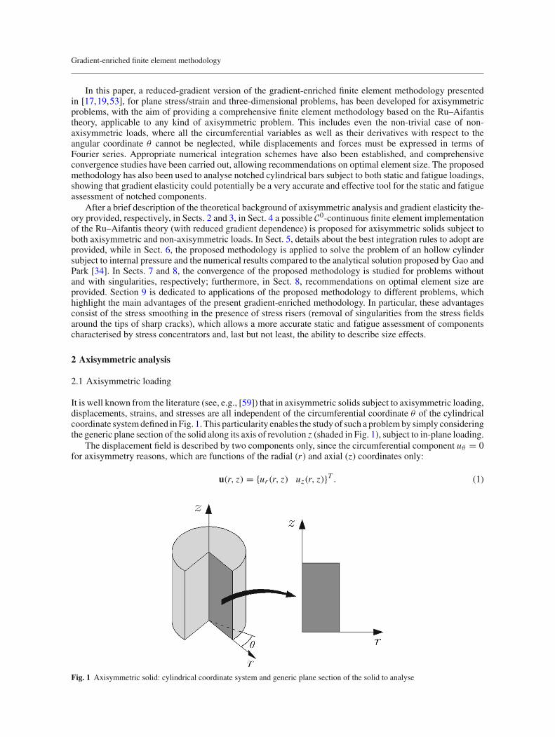
It is well known from the literature (see, e.g., [59]) that in axisymmetric solids subject to axisymmetric loading,displacements, strains, and stresses are all independent of the circumferential coordinate θ of the cylindricalcoordinate systemdefined in Fig. 1. This particularity enables the study of such a problemby simply consideringthe generic plane section of the solid along its axis of revolution z (shaded in Fig. 1), subject to in-plane loading.

The displacement field is described by two components only, since the circumferential component uθ = 0for axisymmetry reasons, which are functions of the radial (r ) and axial (z) coordinates only:

u(r, z) = {ur (r, z) uz(r, z)}T . (1)

Fig. 1 Axisymmetric solid: cylindrical coordinate system and generic plane section of the solid to analyse

C. Bagni et al.

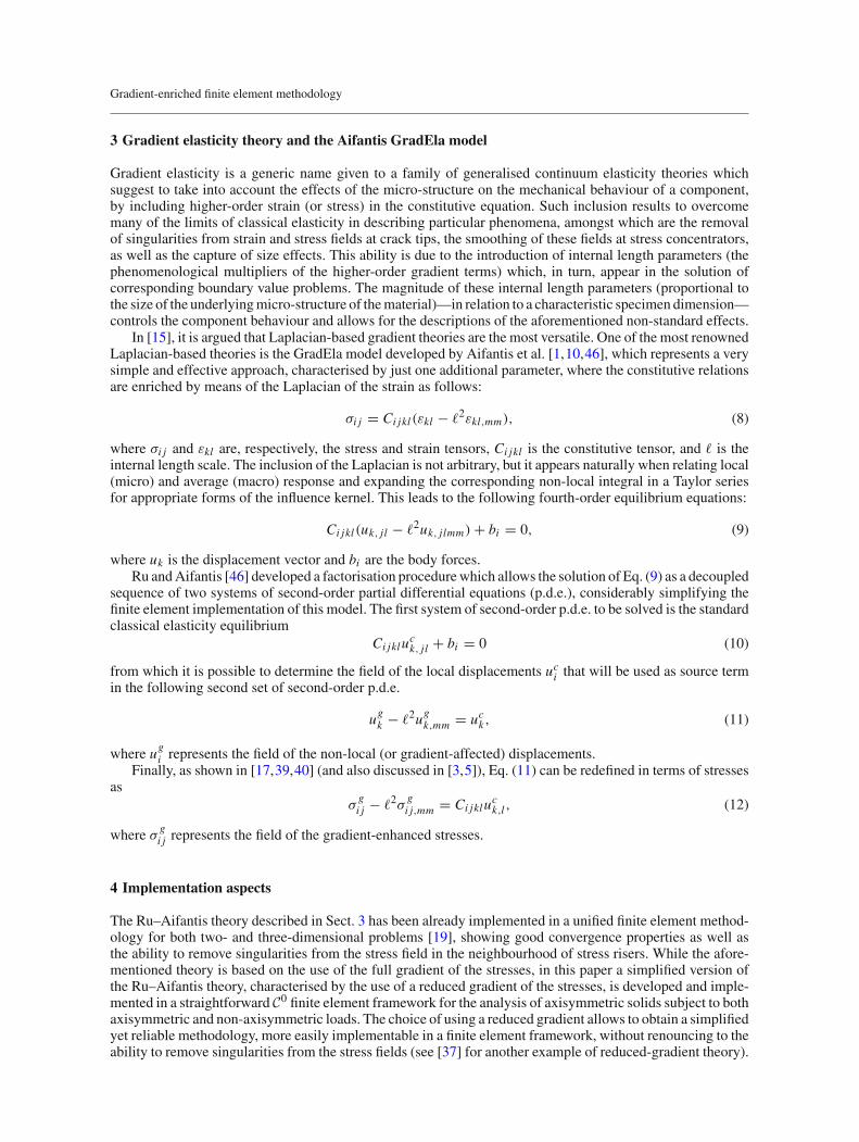
In what concerns the strains, they can be collected in the strain vector

ε(r, z) = {εrr (r, z) εzz(r, z) εθθ (r, z) 2εr z(r, z)}T , (2)

where (ignoring the spatial dependence for notational simplicity)

εrr = ∂ur∂r

, εzz = ∂uz∂z

, εθθ = urr

, 2εr z = ∂uz∂r

+ ∂ur∂z

. (3)

Finally, in the case of linear elastic materials, the stress field is linked to the strain field through the followingconstitutive relation:

σ =

⎧⎪⎪⎪⎪⎨

⎪⎪⎪⎪⎩

σrr

σzz

σθθ

σr z

⎫⎪⎪⎪⎪⎬

⎪⎪⎪⎪⎭

= Cε = E

(1 + ν)(1 − 2ν)

⎡

⎢⎢⎢⎢⎣

1 − ν ν ν 0

ν 1 − ν ν 0

ν ν 1 − ν 0

0 0 0 1−2ν2

⎤

⎥⎥⎥⎥⎦

ε, (4)

where E and ν are the Young’s modulus and Poisson’s ratio, respectively.

2.2 Non-axisymmetric loading

In the case of an axisymmetric solid subject to non-axisymmetric loads, the circumferential component of thedisplacements uθ must be taken into account in addition to the radial and axial components. As a consequenceof this, none of the strain and stress components can be considered null; in particular, the strain vector assumesthe following form (ignoring the spatial dependence for notational simplicity)

ε = {εrr εzz εθθ 2εr z 2εrθ 2εzθ }T , (5)

where in addition to Eq. (3), we have

2εrθ = 1

r

(∂ur∂θ

− uθ

)

+ ∂uθ

∂r, 2εzθ = ∂uθ

∂z+ 1

r

∂uz∂θ

, (6)

and the stress vector is now defined as

σ =

⎧⎪⎪⎪⎪⎪⎪⎪⎪⎪⎨

⎪⎪⎪⎪⎪⎪⎪⎪⎪⎩

σrr

σzz

σθθ

σr z

σrθ

σzθ

⎫⎪⎪⎪⎪⎪⎪⎪⎪⎪⎬

⎪⎪⎪⎪⎪⎪⎪⎪⎪⎭

= C�ε = E

(1 + ν)(1 − 2ν)

⎡

⎢⎢⎢⎢⎢⎢⎢⎢⎢⎢⎣

1 − ν ν ν 0 0 0

ν 1 − ν ν 0 0 0

ν ν 1 − ν 0 0 0

0 0 0 1−2ν2 0 0

0 0 0 0 1−2ν2 0

0 0 0 0 0 1−2ν2

⎤

⎥⎥⎥⎥⎥⎥⎥⎥⎥⎥⎦

ε. (7)

However, it is still possible to solve this problem as a quasi-bidimensional problem by expressing the load anddisplacement components through Fourier series (see, e.g. [58,60]).

Gradient-enriched finite element methodology

3 Gradient elasticity theory and the Aifantis GradEla model

Gradient elasticity is a generic name given to a family of generalised continuum elasticity theories whichsuggest to take into account the effects of the micro-structure on the mechanical behaviour of a component,by including higher-order strain (or stress) in the constitutive equation. Such inclusion results to overcomemany of the limits of classical elasticity in describing particular phenomena, amongst which are the removalof singularities from strain and stress fields at crack tips, the smoothing of these fields at stress concentrators,as well as the capture of size effects. This ability is due to the introduction of internal length parameters (thephenomenological multipliers of the higher-order gradient terms) which, in turn, appear in the solution ofcorresponding boundary value problems. The magnitude of these internal length parameters (proportional tothe size of the underlyingmicro-structure of thematerial)—in relation to a characteristic specimen dimension—controls the component behaviour and allows for the descriptions of the aforementioned non-standard effects.

In [15], it is argued that Laplacian-based gradient theories are the most versatile. One of the most renownedLaplacian-based theories is the GradEla model developed by Aifantis et al. [1,10,46], which represents a verysimple and effective approach, characterised by just one additional parameter, where the constitutive relationsare enriched by means of the Laplacian of the strain as follows:

σi j = Ci jkl(εkl − �2εkl,mm), (8)

where σi j and εkl are, respectively, the stress and strain tensors, Ci jkl is the constitutive tensor, and � is theinternal length scale. The inclusion of the Laplacian is not arbitrary, but it appears naturally when relating local(micro) and average (macro) response and expanding the corresponding non-local integral in a Taylor seriesfor appropriate forms of the influence kernel. This leads to the following fourth-order equilibrium equations:

Ci jkl(uk, jl − �2uk, jlmm) + bi = 0, (9)

where uk is the displacement vector and bi are the body forces.Ru andAifantis [46] developed a factorisation procedurewhich allows the solution of Eq. (9) as a decoupled

sequence of two systems of second-order partial differential equations (p.d.e.), considerably simplifying thefinite element implementation of this model. The first system of second-order p.d.e. to be solved is the standardclassical elasticity equilibrium

Ci jkluck, jl + bi = 0 (10)

from which it is possible to determine the field of the local displacements uci that will be used as source termin the following second set of second-order p.d.e.

ugk − �2ugk,mm = uck, (11)

where ugi represents the field of the non-local (or gradient-affected) displacements.Finally, as shown in [17,39,40] (and also discussed in [3,5]), Eq. (11) can be redefined in terms of stresses

asσgi j − �2σ

gi j,mm = Ci jklu

ck,l , (12)

where σgi j represents the field of the gradient-enhanced stresses.

4 Implementation aspects

The Ru–Aifantis theory described in Sect. 3 has been already implemented in a unified finite element method-ology for both two- and three-dimensional problems [19], showing good convergence properties as well asthe ability to remove singularities from the stress field in the neighbourhood of stress risers. While the afore-mentioned theory is based on the use of the full gradient of the stresses, in this paper a simplified version ofthe Ru–Aifantis theory, characterised by the use of a reduced gradient of the stresses, is developed and imple-mented in a straightforward C0 finite element framework for the analysis of axisymmetric solids subject to bothaxisymmetric and non-axisymmetric loads. The choice of using a reduced gradient allows to obtain a simplifiedyet reliable methodology, more easily implementable in a finite element framework, without renouncing to theability to remove singularities from the stress fields (see [37] for another example of reduced-gradient theory).

C. Bagni et al.

4.1 Axisymmetric loads

The index notation used in Sect. 3 is valid in Cartesian coordinates, while axisymmetric problems are usuallyaddressed in cylindrical coordinates as in the following of the present paper. Therefore, in order to derivethe finite element equations for axisymmetric problems unambiguously, we will now depart from the indexnotation used in the previous section, adopting a tensorial notation. Furthermore, two functionals, one for eachof the two steps of the Ru–Aifantis theory, are defined as follows:

W1 =∫

Ω

1

2εcTCεc dΩ −

∫

Ω

ucTb dΩ −∫

n

ucT t dn (13)

for the first step and

W2 =∫

Ω

1

2

[

σ gTSσ g + �2(

∂σ gT

∂rS

∂σ g

∂r+ ∂σ gT

∂zS

∂σ g

∂z

)]

dΩ −∫

Ω

σ gT εc dΩ (14)

for the second, where uc and εc are, respectively, the local displacement and local strain vectors, σ g is thenon-local stress vector, C is the constitutive matrix, defined in Eq. (4), S = C−1 is the compliance matrix, bis the vector of the body forces in the domain Ω , t is the vector of the prescribed traction on the free portionn of the boundary.

Imposing the stationarity of the first functional, that is, δW1 = 0, the usual global system of standardelasticity equations is obtained:

Kdc − f = 0, (15)

where dc is the vector of the nodal local displacements, K = ∫

ΩBTu CBudΩ is the stiffness matrix and

f = ∫

ΩNTu b dΩ − ∫

nNTu t dn the force vector.

Repeating the same procedure for the second functional, W2, leads to

∫

Ω

NTσ Nσ + �2

(∂NT

σ

∂r

∂Nσ

∂r+ ∂NT

σ

∂z

∂Nσ

∂z

)

dΩ sg −∫

Ω

NTσ Bu dΩ dc = 0, (16)

where sg is the vector of the nodal non-local stresses and Nσ is just an expanded version of the shape functionmatrix Nu , in order to accommodate all four non-local stress components, so that σ g = Nσ sg .

At this point, solving Eq. (15) for dc, and using the result as source term in Eq. (16), the nodal values ofthe gradient-enriched stresses sg can be easily calculated.

4.2 Non-axisymmetric loads

The finite element equations for the case of axisymmetric solids subject to non-axisymmetric loads can bedetermined by following the same process described in Sect. 4.1.

Regarding the first step of the Ru–Aifantis theory, the functional defined by Eq. (13) can be considered bytaking into account that now the constitutive matrix is C� defined in Eq. (7) and the displacements (includingnow also the circumferential component) are described by means of Fourier series as

uc =m∑

h=0

ΘshNud

c,sh +

m∑

h=0

ΘahNud

c,ah (17)

with

Θsh =

⎡

⎢⎢⎣

cos(hθ) 0 0

0 cos(hθ) 0

0 0 sin(hθ)

⎤

⎥⎥⎦ and Θa

h =

⎡

⎢⎢⎣

sin(hθ) 0 0

0 sin(hθ) 0

0 0 cos(hθ)

⎤

⎥⎥⎦ , (18)

where h is the order of the harmonic, while the superscripts s and a indicate, respectively, the symmetric andanti-symmetric components of the displacements (and of the loads) with respect to the θ = 0 axis.

Gradient-enriched finite element methodology

The local strains are defined as follows:

εc =

⎧⎪⎪⎪⎪⎪⎪⎪⎪⎪⎪⎨

⎪⎪⎪⎪⎪⎪⎪⎪⎪⎪⎩

εcrr

εczz

εcθθ

εcrz

εcrθ

εczθ

⎫⎪⎪⎪⎪⎪⎪⎪⎪⎪⎪⎬

⎪⎪⎪⎪⎪⎪⎪⎪⎪⎪⎭

= Luc =

⎡

⎢⎢⎢⎢⎢⎢⎢⎢⎢⎢⎢⎣

∂∂r 0 0

0 ∂∂z 0

1r 0 1

r∂∂θ

∂∂z

∂∂r 0

1r

∂∂θ

0 ∂∂r − 1

r

0 1r

∂∂θ

∂∂z

⎤

⎥⎥⎥⎥⎥⎥⎥⎥⎥⎥⎥⎦

⎧⎪⎨

⎪⎩

ucr

ucz

ucθ

⎫⎪⎬

⎪⎭, (19)

and substituting Eq. (17) into (19)

εc =m∑

h=0

Bsu,hd

c,sh +

m∑

h=0

Bau,hd

c,ah , (20)

where Bsu,h = LΘs

hNu and Bau,h = LΘa

hNu are the two strain-displacement matrices for symmetric andantisymmetric displacements/loads, respectively.

After these considerations, the first step of the Ru–Aifantis theory still consists in Eq. (15), with thedifference that now also the nodal forces are expressed in terms of Fourier series as

f =

⎧⎪⎨

⎪⎩

fr

fz

fθ

⎫⎪⎬

⎪⎭=

⎧⎪⎪⎪⎪⎪⎪⎪⎪⎨

⎪⎪⎪⎪⎪⎪⎪⎪⎩

m∑

h=0f sr,h cos(hθ) +

m∑

h=0f ar,h sin(hθ)

m∑

h=0f sz,h cos(hθ) +

m∑

h=0f az,h sin(hθ)

m∑

h=0f sθ,h sin(hθ) +

m∑

h=0f aθ,h cos(hθ)

⎫⎪⎪⎪⎪⎪⎪⎪⎪⎬

⎪⎪⎪⎪⎪⎪⎪⎪⎭

, (21)

and the stiffness matrix is defined as

K =m∑

h=0

m∑

l=0

khl , (22)

where khl is the stiffness contribution of the hth and lth harmonics, given by

khl =∫

V

BTu,hC

�Bu,ldV =∫

V

[BsTu,h

BaTu,h

]

C�[Bsu,l B

au,l

]dV

=∫

V

[BsTu,hC

�Bsu,l B

sTu,hC

�Bau,l

BaTu,hC

�Bsu,l B

aTu,hC

�Bau,l

]

dV .

(23)

Considering that dV = rdrdzdθ = rdθdA, it can be easily demonstrated that

∫

A

2π∫

0

BsTu,hC

�Bau,l rdθdA =

∫

A

2π∫

0

BaTu,hC

�Bsu,l rdθdA = [0] , (24)

which means that the symmetric and anti-symmetric terms are decoupled, as it should be, given the orthogo-nality of the Fourier series. Furthermore, it can also be proved that

∫

A

2π∫

0

BsTu,hC

�Bsu,l rdθdA =

∫

A

2π∫

0

BaTu,hC

�Bau,l rdθdA = [0] when h �= l. (25)

C. Bagni et al.

Hence, the off-diagonal terms of the global stiffness matrix K are all null and each harmonic can be treatedseparately, allowing application of the principle of superposition to determine the final result.

In what concerns the second step of the Ru–Aifantis theory, considering for simplicity only the symmetriccomponents, defining the following functional:

W̃2 =∫

V

1

2

⎧⎨

⎩

(Θs

σ,hσg,sh

)T S�(Θs

σ,hσg,sh

) + �2

⎡

⎣

(

Θsσ,h

∂σg,sh

∂r

)T

S�

(

Θsσ,h

∂σg,sh

∂r

)

+

+(

Θsσ,h

∂σg,sh

∂z

)T

S�

(

Θsσ,h

∂σg,sh

∂z

)

+ 1

r

∂

∂θ

(Θs

σ,hσg,sh

)T S� 1

r

∂

∂θ

(Θs

σ,hσg,sh

)

⎤

⎦

⎫⎬

⎭dV−

−∫

V

(Θs

σ,hσg,sh

)Tεc,sh dV,

(26)

where S� = C�−1, while Θsσ,h is defined as (see, e.g. [58])

Θsσ,h =

⎡

⎢⎢⎢⎢⎢⎢⎢⎢⎢⎢⎣

cos(hθ) 0 0 0 0 0

0 cos(hθ) 0 0 0 0

0 0 cos(hθ) 0 0 0

0 0 0 cos(hθ) 0 0

0 0 0 0 sin(hθ) 0

0 0 0 0 0 sin(hθ)

⎤

⎥⎥⎥⎥⎥⎥⎥⎥⎥⎥⎦

, (27)

and imposing the stationarity of W̃2, that is, δW̃2 = 0, the following solving system of equations is obtained:

∫

V

[

NTσ ΘsT

h ΘshNσ + �2

(∂NT

σ

∂rΘsT

h Θsh∂Nσ

∂r+ ∂NT

σ

∂zΘsT

h Θsh∂Nσ

∂z

+ 1

r2NT

σ

∂ΘsTh

∂θ

∂Θsh

∂θNσ

)]

dV sg,sh =∫

V

NTσ ΘsT

h CBsu,hdV dc,sh ,

(28)

which can be easily numerically solved for the non-local stress sg,sh . The same system must be solved alsofor the anti-symmetric components (if needed). Finally, once the solutions for all the necessary harmonics arecalculated, the global solution can be determined through superposition of the effects.

5 Numerical integration

For the numerical solution of Eqs. (15), (16), and (28), the Gauss quadrature rule has been used. As summarisedin Table 1, in what concerns Eq. (15) (first step), since it coincides with the p.d.e. of classical elasticity, the stan-dard number of integration points has been considered, in particular the bi-quadratic serendipity quadrilateralshave been under-integrated.

For the numerical solution of Eqs. (16) (second step with axisymmetric loads) and (28) (second step withnon-axisymmetric loads), instead, higher integration rules are needed, except for the bi-linear quadrilateralelements, if � = 0 (as reported in Table 1). On the other hand, if � �= 0, the quadrature rules used for thefirst step can be adopted for all the elements without any rank deficiency problem, similar to the 2D planestrain/stress and 3D problems, as described in [19].

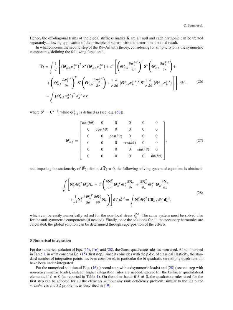
Gradient-enriched finite element methodology

Table 1 Number of Gauss points used in the first step of the Ru-Aifantis theory and formally required in the second step (when� = 0)

Elements Order Gauss points

1st step Triangles Linear 1Quadratic 3

Quadrilaterals Bi-linear 2 × 2Bi-quadratic 2 × 2

2nd step Triangles Linear 3Quadratic 6 (degree of precision 4)

Quadrilaterals Bi-linear 2 × 2Bi-quadratic 3 × 3

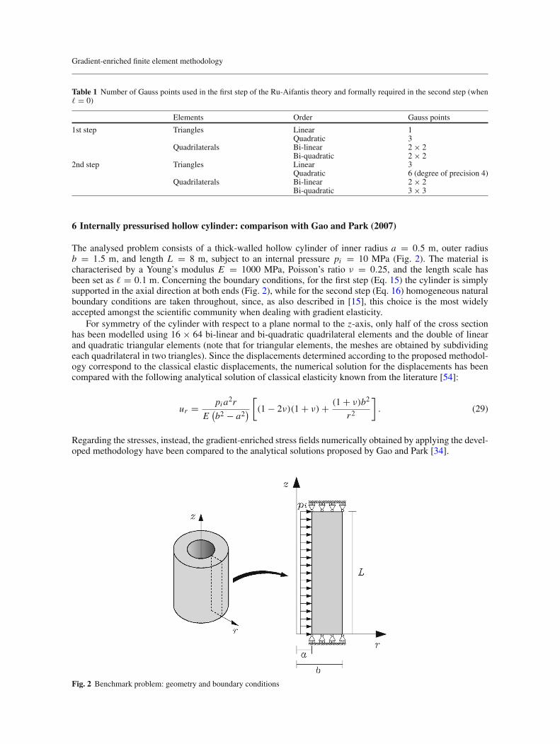
6 Internally pressurised hollow cylinder: comparison with Gao and Park (2007)

The analysed problem consists of a thick-walled hollow cylinder of inner radius a = 0.5 m, outer radiusb = 1.5 m, and length L = 8 m, subject to an internal pressure pi = 10 MPa (Fig. 2). The material ischaracterised by a Young’s modulus E = 1000 MPa, Poisson’s ratio ν = 0.25, and the length scale hasbeen set as � = 0.1 m. Concerning the boundary conditions, for the first step (Eq. 15) the cylinder is simplysupported in the axial direction at both ends (Fig. 2), while for the second step (Eq. 16) homogeneous naturalboundary conditions are taken throughout, since, as also described in [15], this choice is the most widelyaccepted amongst the scientific community when dealing with gradient elasticity.

For symmetry of the cylinder with respect to a plane normal to the z-axis, only half of the cross sectionhas been modelled using 16 × 64 bi-linear and bi-quadratic quadrilateral elements and the double of linearand quadratic triangular elements (note that for triangular elements, the meshes are obtained by subdividingeach quadrilateral in two triangles). Since the displacements determined according to the proposed methodol-ogy correspond to the classical elastic displacements, the numerical solution for the displacements has beencompared with the following analytical solution of classical elasticity known from the literature [54]:

ur = pia2r

E(b2 − a2

)

[

(1 − 2ν)(1 + ν) + (1 + ν)b2

r2

]

. (29)

Regarding the stresses, instead, the gradient-enriched stress fields numerically obtained by applying the devel-oped methodology have been compared to the analytical solutions proposed by Gao and Park [34].

Fig. 2 Benchmark problem: geometry and boundary conditions

C. Bagni et al.

0.5 0.7 0.9 1.1 1.3 1.53

4

5

6

7

8 x 10−3

r [m]

u r [m]

Classical elasticityProposed methodology

0.5 0.7 0.9 1.1 1.3 1.5−8

−6

−4

−2

0 x 106

r [m]

σ rr [P

a]

Gao and Park (2007)Proposed methodology

0.5 0.7 0.9 1.1 1.3 1.52

4

6

8

10

12 x 106

r [m]

σ θθ [P

a]

Gao and Park (2007)Proposed methodology

0.5 0.7 0.9 1.1 1.3 1.50.2

0.6

1

1.4

1.8 x 106

r [m]

σ zz [P

a]

Gao and Park (2007)Proposed methodology

Fig. 3 Comparison between the numerical solutions obtained with bi-quadratic quadrilateral elements and their correspondentanalytical counterparts

In Fig. 3, the displacement and stress fields, obtained by using bi-quadratic quadrilateral elements, arecompared with the relative analytical solutions. Similar results have also been obtained with all the otherimplemented elements.

FromFig. 3, it canbeobserved that the numerical estimationof the radial displacementsur perfectlymatchesthe correspondent analytical counterpart. Regarding the stress components, instead, the numerical solutionsobtained by applying the proposed methodology show some differences when compared with the analyticalsolutions proposed by Gao and Park [34]. In particular, it is possible to observe that both the numerical σ g

θθ andσgzz stress profiles present qualitative and quantitative differences if compared to their analytical counterparts.

This is due to the fact that while the methodology presented in this paper is stress-based, the analyticalsolutions proposed by Gao and Park [34] are obtained through a displacement-based formulation and thereforethe stress components are calculated following different procedures. Furthermore, the displacement-basedformulation used by Gao and Park [34] requires just two higher-order boundary conditions (in particular, theyset homogeneous natural boundary conditions of the radial stress at the inner andouter surfaces)while the stress-based methodology proposed in this paper requires more higher-order boundary conditions (homogeneousnatural boundary conditions of all the stress components at the inner and outer surfaces have been chosen).Therefore, the aforementioned differences are also due to a different choice of the boundary conditions. Finally,it can be easily explained why σ

gzz obtained by applying the proposed methodology should be constant. To do

so, let us consider first the exact stress solutions of classical elasticity known from the literature [54]:

σrr = pia2

b2 − a2

(

1 − b2

r2

)

, σθθ = pia2

b2 − a2

(

1 + b2

r2

)

, σzz = 2νpia2

b2 − a2. (30)

In particular, it can be observed that σzz is constant along the radial coordinate, and therefore, due to the waythe proposed methodology post-processes the stress fields, the longitudinal stress component is not affectedby any gradient enrichment, leading to σ

gzz = σzz = const.

Only quantitative differences can be seen, instead, in the radial stress component, due to the fact that, whilein the proposed methodology the stress components are uncoupled, in the analytical solution proposed by Gaoand Park [34], the stress components are coupled.

Gradient-enriched finite element methodology

Furthermore, the analytical solution proposed by Gao and Park [34] is obtained through a full gradientmethodology, while, as already explained in Sect. 4, the methodology proposed in the present paper is basedon the use of a reduced gradient.

Due to the aforementioned differences (although justified), the analytical solution proposed by Gao andPark cannot be used as benchmark solution for the convergence study performed in the following section wherethe reference solution will be approximated through Richardson extrapolation [45].

7 Convergence study

The convergence behaviour of the implemented elements in the case of both axisymmetric and non-axisymmetric loads has been studied. For this purpose, the L2-norm error defined as

‖e‖2 = ‖σe − σc‖‖σe‖ , (31)

where σe and σc are, respectively, the extrapolated and calculated values of the stresses, has been plotted againstthe number of degrees of freedom (nDoF). From now on, the reference solutions have been approximatedthrough Richardson extrapolation [45].

As already explained in [19], the stresses are determined as primary variable, by solving the second step ofthe Ru–Aifantis theory (either Eq. (16) or (28)) and not as secondary variables, like in standard finite elementmethodologies based on classical elasticity. This means that, although the error conserves its proportionalitywith the nDoF, the theoretical convergence rate for the stresses is different from the one determined in classicalelasticity. In particular, Helmholtz equations such as Eqs. (16) and (28) are characterised by the followingproportionality [41]:

eσ � O(nDoF)−n+12 = O(nDoF)p, (32)

where n is the polynomial order.Equation (32) clearly shows that the ‖e‖2 – nDoF curve in a bi-logarithmic system of axis is represented

by a straight line, whose slope represents the convergence rate p of the numerical solution to the extrapolatedsolution. In particular, the theoretical convergence rate is p = −1 for linear elements and p = −1.5 forquadratic elements.

In what concerns the case of axisymmetric load, the thick-walled hollow cylinder problem presented inSect. 5 has been considered. The domain has been modelled by using all the implemented elements, startingfrom a 4× 16 mesh and refining the mesh, by doubling the number of elements in both directions 4 times, upto a 64 × 256 mesh. The length parameter has been set as � = 0.1 m.

Regarding the case of axisymmetric solids subject to non-axisymmetric loads, two different problems havebeen analysed. The first one consists of a cylindrical bar of radius R = 1 m and length L = 8 m, subject to abending moment M = 106 Nm (Fig. 4, left), while the second one consists of the same cylinder subject nowto a torsional moment T = 106 Nm (Fig. 4, right). In both cases, Young’s modulus E = 1000 MPa, Poisson’sratio ν = 0.25, and the length scale has been set as � = 0.1 m.

For symmetry of the cylinder with respect to a plane normal to the z-axis, in both cases, only half of thecross section has been modelled (Fig. 4). Also, in this case all the implemented elements have been used todiscretise the domain, starting from a 4× 16 mesh and performing the same mesh refinement described in thecase of axisymmetric loads. Concerning the boundary conditions, in both problems, for the first step (Eq. 15with K defined by Eq. 22), homogeneous essential boundary conditions have been imposed, so that uz = 0(bending problem) and uz = uθ = 0 (torsional problem) along the axis of symmetry (Fig. 4), while for thesecond step (Eq. 28) homogeneous natural boundary conditions have been chosen, as in the previous case.

In Fig. 5, the L2-norm error is plotted against the nDoF in a bi-logarithmic system for the three analysedproblems, fromwhich it is possible to appreciate that all the implemented elements produce numerical solutionscharacterised by convergence rates in good agreement with the theoretical predictions when applied to anykind of axisymmetric problem.

C. Bagni et al.

Fig. 4 Cylindrical bars under pure bending (left) and pure torsion (right): geometry and boundary conditions

Fig. 5 Stress error versus nDoF for internal pressure in hollow cylinder (left) and plain cylindrical bars subject to pure bending(centre) and pure torsion (right). The slope of the lines represents the convergence rate

8 Convergence in the presence of singularities and recommendations on optimum element size

As is well known [1,3,5,10,46], one of the most important abilities of gradient elasticity is the removal ofsingularities from the strain and stress fields such as those obtained at the tips of sharp cracks when classicalelasticity is used. See also the analyses in [15,17,19], as well as a more recent discussion in [6,7]. Since thepresence of cracks reduces drastically the convergence rate of standard finite element methodologies, veryfine meshes are required in the neighbourhood of the stress riser to ensure that convergence of the solution isreached, with significant increasing in computational cost. Hence, the analysis of the convergence behaviour ofthe proposed gradient-enriched finite element methodology is of great interest. Furthermore, an accurate errorestimation has allowed the formulation of recommendations on optimal element size also for axisymmetricfinite elements that together with the recommendations provided in [19] for plane and three-dimensional finiteelements constitutes a complete and useful meshing guideline for gradient-enriched finite elements.

To analyse the aforementioned aspects, three different problems (Fig. 6) consisting of a cylindrical barcharacterised by the presence of a circumferential crack and subject, respectively, to axial load F = 106 N(axisymmetric), bending moment M = 106 Nm, and torque T = 106 Nm (non-axisymmetric loads) havebeen studied. The cylinder has a radius R = 1 m, a length L = 8 m, and the crack is 0.25m deep. Materialproperties, boundary conditions, and meshes are taken as in Sect. 7.

As in Sect. 7, the convergence rate is determined as the slope of the straight line obtained by plotting in abi-logarithmic graph the L2-norm error, defined by Eq. (31), versus the nDoF (Fig. 7). From the literature [59],it is known that in the presence of singularities, the error on classical stresses is proportional to the nDoF as

eσ � O(nDoF)−[min(λ,n)]/2 = O(nDoF)p, (33)

where λ = 0.5 for a nearly closed crack, which leads to a theoretical convergence rate p = −0.25 for bothlinear and quadratic elements.

Gradient-enriched finite element methodology

Fig. 6 Cracked cylindrical bars under uniaxial tensile load (left), pure bending (centre), and pure torsion (right)

Fig. 7 Stress error versus nDoF for cracked cylindrical bars subject to uniaxial tensile load (left), pure bending (centre), and puretorsion (right). The slope of the lines represents the convergence rate

From Fig. 7, it is possible to observe that, when singularities are involved, both linear and quadraticelements show approximatively the same convergence rate (in accordance with Eq. (33)). Furthermore, theproposed gradient-enriched methodology produces a significant improvement in terms of convergence rate; inparticular, the solutions of the three analysed problems are all characterised by a convergence rate almost threetimes higher than the correspondent theoretical value (typical of standard finite element methodology basedon classical elasticity). As already explained in [19], this improvement is due to two main factors:

– removal of singularities from the stress fields;– gradient-enriched stresses are primary variables, instead of secondary variables (as in standard classical

elasticity-based finite element methodologies).

Analysing then the error affecting the numerical solutions (determined through Eq. (31)), it is possible toprovide recommendations on optimal element size. Table 2 summarises the ratios between the element sizeand the length scale � that ensure an error of about 5% or lower. The recommendations summarised in Table 2highlight the fact that using the proposed methodology, even in the presence of singularities, it is possible toobtain accurate solutions using a fairly coarse mesh, reducing consistently the computational efforts.

9 Applications

9.1 Removal of singularities

As already mentioned in Sect. 1, one of the features of the proposed methodology is the ability to removesingularities from the stress field, such as those emerging near the tip of sharp cracks. This ability can be easily

C. Bagni et al.

Table 2 Recommendations on optimal element size to guarantee an error of 5% or lower

Elements Order Element size/�

Triangles Linear 1Quadratic 5/2

Quadrilaterals Bi-linear 3/2Bi-quadratic 5/2

shown by considering the problems presented in Sect. 8 and comparing the stress profiles obtained by applyingthe proposed methodology with those produced by classical elasticity. In Fig. 8, in fact it can be seen that whilethe classical elastic stress fields are characterised by an unbounded peak in correspondence with the cracktip, the gradient-enriched ones converge to a unique finite solution upon mesh refinement (the stress profilespresented in Fig. 8 were obtained by using bi-quadratic quadrilateral elements, similar results are produced byall the other implemented elements).

9.2 Static and fatigue assessment of notched bars

The aforementioned ability to remove singularities, or more in general the stress smoothing in correspon-dence with stress concentrators, leads to more physically realistic results and therefore to more accurate staticand fatigue assessments of components presenting stress risers. In particular, it allows the static and fatigueassessments, by considering the values of the relevant stresses directly at the crack/notch tip and not into theanalysed body, as it happens in most of the existing assessment procedures, with evident simplifications in theassessment process.

In [16,48], similarities and differences between gradient elasticity and the Theory of Critical Distances(TCD) (for an in-depth description of this theory, see [52]) are investigated, showing the advantages of thesetwo theories in the static and fatigue assessment of cracked components. Furthermore, in [48] a relation linkingthe two length parameters, characterising the aforementioned theories has been proposed, namely

� ≈ L

2√2, (34)

where L is the characteristic length of the TCD, defined as in [52].The proposed methodology has been applied to notched cylindrical bars (Fig. 9), subject to both static and

fully reversed cyclic loadings (load ratio R = −1), in order to show the accuracy of the proposedmethodology,with � defined through Eq. (34), in the determination of both static and fatigue strength of notched components(for more results, see also [20]).

The accuracy of the proposed methodology has been tested against a wide range of materials (both brittleand ductile) and notch root radii.

All the relevant data about the analysed problems are summarised in Tables 3 and 4, where σ0 is the inherentmaterial strength, σth is the ultimate tensile nominal stress, Δσ0 is the plain fatigue limit stress range, andΔσth is the range of the nominal fatigue strength (all the nominal stresses are referred to the gross section ofthe specimens).

The accuracy of the proposed methodology in estimating both the static strength and the fatigue limit ofnotched cylindrical bars has been verified by defining the following errors:

error = σeff − σ0

σ0[%] and error = Δσeff − Δσ0

Δσ0[%] (35)

for static and fatigue problems, respectively, where σeff and Δσeff are, respectively, the stress (for staticproblems) and the stress range (for fatigue problems) numerically obtained at the notch tip.

In Fig. 10, the aforementioned errors are plotted for the different analysed materials, from which it ispossible to appreciate the accuracy of the proposed methodology, with errors mainly ranging between −10%and +30% (dashed lines). Considering the usual error band ±20%, it is possible to observe that the presentmethodology produces results with errors falling into a band of the same size, but 10% more conservative.

Gradient-enriched finite element methodology

0 0.2 0.4 0.6 0.8 1−5

0

5

10

15

20 x 105

r [m]

σ zz [P

a]

4x16 elements8x32 elements16x64 elements32x128 elements64x256 elements

0 0.2 0.4 0.6 0.8 1−5

0

5

10

15

20 x 105

r [m]

σg zz [P

a]

4x16 elements8x32 elements16x64 elements32x128elements64x256 elements

0 0.2 0.4 0.6 0.8 1−1

0

1

2

3

4

5

6

7

8 x 106

r [m]

σ zz [P

a]

4x16 elements8x32 elements16x64 elements32x128 elements64x256 elements

0 0.2 0.4 0.6 0.8 1−2

0

2

4

6

8 x 106

r [m]

σg zz [P

a]

4x16 elements8x32 elements16x64 elements32x128 elements64x256 elements

0 0.2 0.4 0.6 0.8 1−1

0

1

2

3

4 x 106

r [m]

τ zθ [P

a]

4x16 elements8x32 elements16x64 elements32x128 elements64x256 elements

0 0.2 0.4 0.6 0.8 1−1

0

1

2

3

4 x 106

r [m]

τg zθ [P

a]

4x16 elements8x32 elements16x64 elements32x128 elements64x256 elements

Fig. 8 Stress profiles obtained by applying classical (left) and gradient (right) elasticity, for uniaxial tensile loading (top), purebending (centre), and pure torsion (bottom)

Fig. 9 Geometry of the cylindrical notched bars

C. Bagni et al.

Table 3 Geometrical and material parameters of the notched cylindrical bars under static loading

Material Ref. Load type σ0 L � D a ρ σth[MPa] [mm] [mm] [mm] [mm] [mm] [MPa]

PMMA [49] Axial 113.9 0.108 0.038 12.8 2.3 0.2 13.8312.8 2.3 0.4 17.3312.8 2.3 1.2 21.6012.8 2.3 4.0 21.99

Al6082 [51] Axial 445.9 1.640 0.580 10.0 1.90 0.44 206.5410.0 1.95 0.50 205.2510.0 1.90 1.25 201.3110.0 1.95 4.00 167.18

Table 4 Geometrical and material parameters of the notched cylindrical bars under fatigue loading. All the values for Δσth aretaken from [18]

Material Ref. Load type Δσ0 L � D a ρ Δσth[MPa] [mm] [mm] [mm] [mm] [mm] [MPa]0.45 C steel [18] Rotating bending 582 0.061 0.022 5.01 0.005 0.05 547

5.01 0.005 0.02 5475.01 0.005 0.01 5575.02 0.01 0.05 4845.02 0.01 0.02 4945.02 0.01 0.01 4845.2 0.1 0.6 3735.2 0.1 0.3 3385.2 0.1 0.1 3025.2 0.1 0.05 3205.2 0.1 0.02 3206 0.5 0.6 2086 0.5 0.3 1746 0.5 0.1 1626 0.5 0.05 1626 0.5 0.02 1686 0.5 0.01 1688 1.5 0.6 85.48 1.5 0.3 68.48 1.5 0.1 61.08 1.5 0.05 61.08 1.5 0.02 61.08 1.5 0.01 63.5

0.36 C steel [18] Rotating bending 446 0.092 0.033 15.0 1.0 0.2 11314.4 0.7 0.2 13614.0 0.5 0.2 16413.6 0.3 0.2 20313.3 0.15 0.2 25513.2 0.1 0.2 290

Mild Steel [47,55] Axial 420 0.296 0.105 43.0 5.08 0.05 68.843.0 5.08 0.10 70.043.0 5.08 0.13 67.743.0 5.08 0.25 68.843.0 5.08 0.64 68.843.0 5.08 1.27 77.043.0 5.08 5.08 121.0

NiCr steel [50] Axial 1000 0.085 0.030 22.6 0.51 0.13 236.043.0 5.08 0.05 88.631.8 5.08 0.13 96.6

Steel 15313 [47,55] Axial 440 0.237 0.084 5.0 0.03 0.03 429.05.0 0.05 0.05 403.05.0 0.07 0.07 321.05.0 0.20 0.20 237.05.0 0.40 0.40 209.05.0 0.76 0.76 155.0

AISI 304 [50] Axial 720 0.110 0.039 43.0 5.08 0.05 72.3

Gradient-enriched finite element methodology

Fig. 10 Error in the estimation of both static strength and fatigue limit of notched cylindrical bars

9.3 Size effects

In previous publications byAifantis et al. [2,4,14,27,28], it was shown that theGradElamodel can convenientlycapture the occurrence of elastic size effects in small one-dimensional objects and specimens with holescommonly used for advanced technology applications. More recently, its extension to describe size effectsdue to thermomechanical, chemomechanical, and electromechanical couplings has been reviewed in [7]. Thepurpose of this section is to expand this discussion for an emerging technological problem of internal stressdevelopment and capacity fade in Lithium-ion (Li-ion) rechargeable battery electrodes by elaborating on theclassical elasticity treatment first used for this problem in the pioneering work of [8] (see also related chaptersand references in [9]).

In fact, nowadays, the majority of electronic devices, such as laptops, tablets, smart phones, and digitalcameras, are powered by Li-ion batteries. Li-ion batteries have replaced their older sisters nickel-cadmium(Ni–Cd) and nickel-metal-hydride (Ni–MH) batteries due to their unique characteristics, such as lightness,high energy density, and non-toxicity [8].

In Li-ion batteries, the active sites in the anode and (to a lesser extent) in the cathode are subject to significantexpansions upon lithium insertion, which leads to a severe damage of the surrounding glass/ceramic matrixand consequently to a deterioration of the electrochemical properties of the electrodes. It is then evident howcritical an accurate estimation of the stresses in the matrix is for a subsequent damage evaluation.

However, the dimensions characterising this problems are usually of the order of nanometres, which makesclassical elasticity not accurate enough for the estimation of the stresses, due to its incapability to capture sizeeffects, particularly significant at the nanoscale. In this section, the proposed gradient-enriched methodologyis applied to study the aforementioned problem, in order to show its ability to easily describe size effects,obtaining a more accurate size-dependent estimation of the stresses, with a small additional computationaleffort.

The active sites of the electrodes can be fabricated in different shapes like thin layers, spheres, or fibres.In this section, the third shape is considered and analysed.

Fibre-like electrodes can be considered as a series of unit cells formed by a cylindrical Li-ion active siteof radius r = a, surrounded by a glass or ceramic matrix (inert with respect to Li) of radius r = b.

Two different problems have been analysed: in first instance, only the outer matrix has been modelled as anhollow cylinder, and after that, both the active site and the surroundingmatrix have beenmodelled as two nestedcylinder made of two different materials. The material properties are taken as Eg = 75 GPa, Es = 41 GPa,νg = 0.25, and νs = 0.33 (see [8]), where the subscript g refers to the glass matrix and the subscript s to theactive site. Furthermore, the glass matrix and the active site are characterised by an internal length �g and �s ,respectively. Concerning the geometry dimensions, the inner and outer radii have been defined, respectively,as a = γ a0 and b = γ b0, where a0 and b0 are, respectively, the inner and outer radii of the domain, as given in

C. Bagni et al.

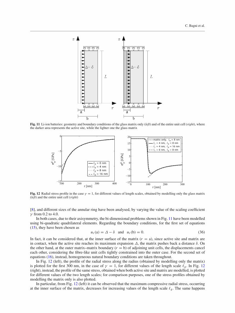
Fig. 11 Li-ion batteries: geometry and boundary conditions of the glass matrix only (left) and of the entire unit cell (right), wherethe darker area represents the active site, while the lighter one the glass matrix

100 200 300 400−15

−10

−5

0

r [nm]

σg rr [G

Pa]

g = 0 nmg = 4 nmg = 8 nmg = 16 nm

0 100 200 300−15

−10

−5

0

5

10

15

20

r [nm]

σg rr [G

Pa]

matrix only, g = 8 nms = 4 nm, g = 8 nms = 4 nm, g = 16 nms = 6 nm, g = 8 nm

Fig. 12 Radial stress profile in the case γ = 1, for different values of length scales, obtained by modelling only the glass matrix(left) and the entire unit cell (right)

[8], and different sizes of the annular ring have been analysed, by varying the value of the scaling coefficientγ from 0.2 to 4.0.

In both cases, due to their axisymmetry, the bi-dimensional problems shown in Fig. 11 have been modelledusing bi-quadratic quadrilateral elements. Regarding the boundary conditions, for the first set of equations(15), they have been chosen as

ur (a) = Δ − δ and ur (b) = 0. (36)

In fact, it can be considered that, at the inner surface of the matrix (r = a), since active site and matrix arein contact, when the active site reaches its maximum expansion Δ, the matrix pushes back a distance δ. Onthe other hand, at the outer matrix–matrix boundary (r = b) of adjoining unit cells, the displacements canceleach other, considering the fibre-like unit cells tightly constrained into the outer case. For the second set ofequations (16), instead, homogeneous natural boundary conditions are taken throughout.

In Fig. 12 (left), the profile of the radial stress along the radius (obtained by modelling only the matrix)is plotted for the first 300 nm, in the case of γ = 1, for different values of the length scale �g . In Fig. 12(right), instead, the profile of the same stress, obtained when both active site andmatrix are modelled, is plottedfor different values of the two length scales; for comparison purposes, one of the stress profiles obtained bymodelling the matrix only is also plotted.

In particular, from Fig. 12 (left) it can be observed that the maximum compressive radial stress, occurringat the inner surface of the matrix, decreases for increasing values of the length scale �g . The same happens

Gradient-enriched finite element methodology

0.3 0.6 0.9 1.2 1.5 1.8−0.1

0

0.1

0.2

0.3

0.4

0.5

Log(a/ g)

Log

(stressratio)

Gradient el. (matrix only)Gradient el. (active site + matrix)Classical el.

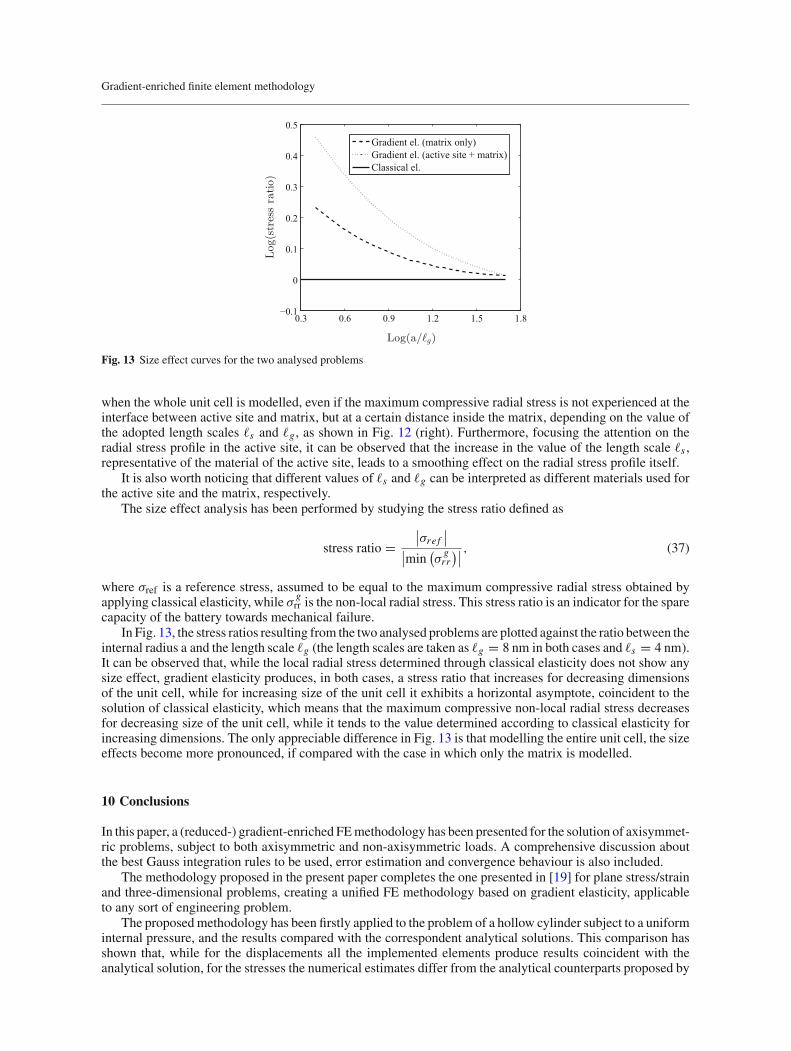
Fig. 13 Size effect curves for the two analysed problems

when the whole unit cell is modelled, even if the maximum compressive radial stress is not experienced at theinterface between active site and matrix, but at a certain distance inside the matrix, depending on the value ofthe adopted length scales �s and �g , as shown in Fig. 12 (right). Furthermore, focusing the attention on theradial stress profile in the active site, it can be observed that the increase in the value of the length scale �s ,representative of the material of the active site, leads to a smoothing effect on the radial stress profile itself.

It is also worth noticing that different values of �s and �g can be interpreted as different materials used forthe active site and the matrix, respectively.

The size effect analysis has been performed by studying the stress ratio defined as

stress ratio =∣∣σre f

∣∣

∣∣min

(σgrr

)∣∣, (37)

where σref is a reference stress, assumed to be equal to the maximum compressive radial stress obtained byapplying classical elasticity, while σ

grr is the non-local radial stress. This stress ratio is an indicator for the spare

capacity of the battery towards mechanical failure.In Fig. 13, the stress ratios resulting from the two analysed problems are plotted against the ratio between the

internal radius a and the length scale �g (the length scales are taken as �g = 8 nm in both cases and �s = 4 nm).It can be observed that, while the local radial stress determined through classical elasticity does not show anysize effect, gradient elasticity produces, in both cases, a stress ratio that increases for decreasing dimensionsof the unit cell, while for increasing size of the unit cell it exhibits a horizontal asymptote, coincident to thesolution of classical elasticity, which means that the maximum compressive non-local radial stress decreasesfor decreasing size of the unit cell, while it tends to the value determined according to classical elasticity forincreasing dimensions. The only appreciable difference in Fig. 13 is that modelling the entire unit cell, the sizeeffects become more pronounced, if compared with the case in which only the matrix is modelled.

10 Conclusions

In this paper, a (reduced-) gradient-enriched FEmethodology has been presented for the solution of axisymmet-ric problems, subject to both axisymmetric and non-axisymmetric loads. A comprehensive discussion aboutthe best Gauss integration rules to be used, error estimation and convergence behaviour is also included.

The methodology proposed in the present paper completes the one presented in [19] for plane stress/strainand three-dimensional problems, creating a unified FE methodology based on gradient elasticity, applicableto any sort of engineering problem.

The proposedmethodology has been firstly applied to the problem of a hollow cylinder subject to a uniforminternal pressure, and the results compared with the correspondent analytical solutions. This comparison hasshown that, while for the displacements all the implemented elements produce results coincident with theanalytical solution, for the stresses the numerical estimates differ from the analytical counterparts proposed by

C. Bagni et al.

Gao and Park [34]. These differences can be ascribed to the fact that while the proposedmethodology is a stress-gradient elastic methodology, the one used by Gao and Park represents a displacement-based formulation, thisleading in particular to different higher-order boundary conditions and different relationship amongst the stresscomponents (while in the analytical solution proposed by Gao and Park the stress components are coupled, inthe developed methodology they are uncoupled). Moreover, whereas Gao and Park [34] in their work use a fullgradient approach, the methodology proposed in the present paper is based on the use of a reduced gradient.

The convergence behaviour of the proposed methodology has been checked in both the absence and thepresence of singularities, for three different loading conditions. The results have shown that for problemswithout singularities, overall, the convergence rates of the numerical solutions are well in line with the cor-respondent theoretical predictions. In the presence of singularities, instead, the convergence rates are higherthan the correspondent theoretical values, typical of traditional finite element methodologies. The cause of thisfaster convergence has been mainly attributed to two aspects:

– the removal of singularities, characteristic of gradient elasticity theories;– the non-local stresses determined as primary variables, instead of secondary variables as in traditional

finite element methodologies.

Furthermore, a guideline on optimal element size has been suggested, highlighting that relatively coarsemeshes can produce sufficiently accurate solutions, with associated reduction in computational costs.

The ability of the proposed methodology to remove singularities from the stress fields has been shown byanalysing three problems, consisting of a cylindrical bar characterised by a circumferential crack and subjectto three different loading conditions.

The accuracy of the present methodology in the static and fatigue assessment of notched cylindrical barshas been also investigated for both brittle and ductile materials, covering a wide range of notch root radiias well. This study has shown that the proposed gradient-enriched FE methodology produces very accurateresults, with errors ranging from−10% and+30%, which correspond to an error band equal to the usual±20%but shifted 10% towards the conservative side. In addition, the proposed methodology allows the static andfatigue assessment of cracked/notched components by considering the relevant stress values directly at the tipof the stress riser (i.e. on the surface), avoiding the need to know a priori the failure location into the body, withevident advantages from an industrial point of view. Thus, it is possible to state that the proposed methodologycan potentially become a powerful tool in the static and fatigue assessment of components presenting stressconcentrators.

Finally, the proposed finite element methodology has been applied to evaluate the radial stress inside theglass/ceramic matrix surrounding the active sites in the electrodes of Li-ion batteries, showing the ability ofgradient elasticity to describe size effects, or in other words the different mechanical behaviours of the matrixwhen the dimensions of the unit cell are scaled; in particular, it has been pointed out that scale effects becomemore significant for decreasing dimensions of the unit cell.

Thus, it is possible to conclude that, using gradient elasticity, with a limited additional computational costwith respect to classical elasticity, it is possible to take into account size effects, obtaining more accurateestimations of the stresses experienced by the matrix. Furthermore, this feature of gradient elasticity enablesa more accurate choice of the material to use for the matrix (different materials mean different length scales)as well as the most appropriate dimensions of the unit cell.

In a similar way, gradient elasticity can be also employed to consider size effects for the benchmarkproblems presented in [9] to obtain input for the most favourable configurations (spheres vs. cylindrical fibres)and material selection for preventing fracture. Some interesting results are also expected by considering theparameters Δ and δ as being dependent on the concentration of the diffusing Li-ions. This will be discussedindependently in a forthcoming paper.

Acknowledgements The authors gratefully acknowledge financial support from Safe Technology Ltd. (part of the DessaultSistèmes SIMULIA brand), Hellenic ERC-13 and ARISTEIA II projects of the General Secretariat of Research and Technology(GSRT) of Greece. Discussions with Katerina Aifantis who suggested the Li-ion problem are also gratefully acknowledged.

Open Access This article is distributed under the terms of the Creative Commons Attribution 4.0 International License (http://creativecommons.org/licenses/by/4.0/), which permits unrestricted use, distribution, and reproduction in any medium, providedyou give appropriate credit to the original author(s) and the source, provide a link to the Creative Commons license, and indicateif changes were made.

Gradient-enriched finite element methodology

References

1. Aifantis, E.C.: On the role of gradients in the localization of deformation and fracture. Int. J. Eng. Sci. 30(10), 1279–1299(1992). doi:10.1016/0020-7225(92)90141-3

2. Aifantis, E.C.: Strain gradient interpretation of size effects. Int. J. Fract. 95, 299–314 (1999). doi:10.1023/A:10186250068043. Aifantis, E.C.: Update on a class of gradient theories.Mech.Mater. 35, 259–280 (2003). doi:10.1016/S0167-6636(02)00278-

84. Aifantis, E.C.: Exploring the applicability of gradient elasticity to certainmicro/nano reliability problems.Microsyst. Technol.

15(1), 109–115 (2009). doi:10.1007/s00542-008-0699-85. Aifantis, E.C.: On the gradient approach—relation to Eringen’s nonlocal theory. Int. J. Eng. Sci. 49(12), 1367–1377 (2011).

doi:10.1016/j.ijengsci.2011.03.0166. Aifantis, E.C.: On non-singular GRADELA crack fields. Theor. Appl. Mech. Lett. 4(051005), 1–7 (2014). doi:10.1063/2.

14051057. Aifantis, E.C.: Internal length gradient (ILG) mechanics across scales and disciplines. Adv. Appl. Mech. 49, 1–110 (2016).

doi:10.1016/bs.aams.2016.08.0018. Aifantis, K.E., Hackney, S.A.: An ideal elasticity problem for Li-batteries. J. Mech. Behav. Mater. 14(6), 413–427 (2003).

doi:10.1515/JMBM.2003.14.6.4139. Aifantis, K.E., Hackney, S.A., Kumar, V.R. (eds.): High Energy Density Lithium Batteries: Materials, Engineering, Appli-

cations. Wiley, Weinheim (2010)10. Altan, S., Aifantis, E.C.: On the structure of the mode III crack-tip in gradient elasticity. Scr. Metall. Mater. 26, 319–324

(1992). doi:10.1016/0956-716X(92)90194-J. [See also: S. B. Altan, E. C. Aifantis. On some aspects in the special theory ofgradient elasticity. Journal of the Mechanical Behavior of Materials, 8:231–282, 1997]

11. Altan, S., Aifantis, E.C.: On some aspects in the special theory of gradient elasticity. J. Mech. Behav. Mater. 8(3), 231–282(1997). doi:10.1515/JMBM.1997.8.3.231

12. Aravas, N.: Plane-strain problems for a class of gradient elasticity models—a stress function approach. J. Elast. 104(1),45–70 (2011). doi:10.1007/s10659-011-9308-7

13. Argyris, J.: Energy theorems and structural analysis. Aircr. Eng. Aerosp. Technol. 26(11), 383–394 (1954). doi:10.1108/eb032491

14. Askes, H., Aifantis, E.C.: Numerical modeling of size effects with gradient elasticity—formulation, meshless discretizationand examples. Int. J. Fract. 117(4), 347–358 (2002). doi:10.1023/A:1022225526483

15. Askes, H., Aifantis, E.C.: Gradient elasticity in statics and dynamics: an overview of formulations, length scale identificationprocedures, finite element implementations and new results. Int. J. Solids Struct. 48(13), 1962–1990 (2011). doi:10.1016/j.ijsolstr.2011.03.006

16. Askes, H., Livieri, P., Susmel, L., Taylor, D., Tovo, R.: Intrinsic material length, theory of critical distances and gradientmechanics: analogies and differences in processing linear-elastic crack tip stress fields. Fatigue Fract. Eng. Mater. Struct. 36,39–55 (2013). doi:10.1111/j.1460-2695.2012.01687.x

17. Askes,H.,Morata, I., Aifantis, E.C.: Finite element analysiswith staggered gradient elasticity. Comput. Struct. 86, 1266–1279(2008). doi:10.1016/j.compstruc.2007.11.002

18. Aztori, B., Lazzarin, P., Meneghetti, G.: Fracture mechanics and notch sensitivity. Fatigue Fract. Eng. Mater. Struct. 26,257–267 (2003). doi:10.1046/j.1460-2695.2003.00633.x

19. Bagni, C., Askes, H.: Unified finite element methodology for gradient elasticity. Comput. Struct. 160, 100–110 (2015).doi:10.1016/j.compstruc.2015.08.008

20. Bagni, C., Askes, H., Susmel, L.: Gradient elasticity: a transformative stress analysis tool to design notched componentsagainst uniaxial/multiaxial high-cycle fatigue. Fatigue Fract. Eng. Mater. Struct. 39(8), 1012–1029 (2016). doi:10.1111/ffe.12447

21. Bleustein, J.L.: Effects of micro-structure on the stress concentration at a spherical cavity. Int. J. Solids Struct. 2(1), 82–104(1966). doi:10.1016/0020-7683(66)90008-4

22. Cauchy, A.: Mémoire sur les systèmes isotropes de points matériels. In: Oeuvres complètes, 1re Série—Tome II. Gauthier-Villars (reprint 1908), Paris, pp. 351–386 (1850)

23. Cauchy, A.: Mémoire sur les vibrations d’un double système de molécules et de l’éther continu dans un corps cristallisé. In:Oeuvres complètes, 1re Série—Tome II. Gauthier-Villars (reprint 1908), Paris, pp. 338–350 (1850)

24. Cauchy, A.: Note sur l’équilibre et les mouvements vibratoires des corps solides. In: Oeuvres complètes, 1re Série—TomeXI. Gauthier-Villars (reprint 1899), Paris, pp. 341–346 (1851)

25. Cook, T.S., Weitsman, Y.: Strain-gradient effects around spherical inclusions and cavities. Int. J. Solids Struct. 2(3), 393–406(1966). doi:10.1016/0020-7683(66)90029-1

26. Cosserat, E., Cosserat, F.: Théorie des corps déformables. Librairie Scientifique A. Hermann et Fils, Paris (1909)27. Efremidis, G., Carpinteri, A., Aifantis, E.C.: Multifractal scaling law versus gradient elasticity in the evaluation of disordered

material compressive strength. J. Mech. Behav. Mater. 12(2), 107–120 (2001). doi:10.1515/JMBM.2001.12.2.10728. Efremidis, G., Pugno, N., Aifantis, E.C.: A proposition for a “self-consistent” gradient elasticity. J. Mech. Behav. Mater.

19(1), 15–30 (2009). doi:10.1515/JMBM.2009.19.1.1529. Eringen, A.C.: Linear theory of nonlocal elasticity and dispersion of plane waves. Int. J. Eng. Sci. 10(5), 425–435 (1972).

doi:10.1016/0020-7225(72)90050-X30. Eringen, A.C.: Nonlocal polarelastic continua. Int. J. Eng. Sci. 10(1), 1–16 (1972). doi:10.1016/0020-7225(72)90070-531. Eringen, A.C.: On differential equations of nonlocal elasticity and solutions of screw dislocation and surface waves. J. Appl.

Phys. 54(9), 4703–4710 (1983). doi:10.1063/1.33280332. Eshel, N.N.: Axi-symmetric problems in elastic materials of grade two. J. Franklin Inst. 299(1), 43–51 (1975). doi:10.1016/

0016-0032(75)90083-633. Eshel, N.N., Rosenfeld, G.: Effects of strain-gradient on the stress-concentration at a cylindrical hole in a field of uniaxial

tension. J. Eng. Math. 4(2), 97–111 (1970). doi:10.1007/BF01535082

C. Bagni et al.

34. Gao, X.L., Park, S.K.: Variational formulation of a simplified strain gradient elasticity theory and its application to apressurized thick-walled cylinder problem. Int. J. Solids Struct. 44, 7486–7499 (2007). doi:10.1016/j.ijsolstr.2007.04.022

35. Georgiadis, H.G., Anagnostou, D.S.: Problems of the Flamant-Boussinesq and Kelvin type in dipolar gradient elasticity. J.Elast. 90(1), 71–98 (2008). doi:10.1007/s10659-007-9129-x

36. Georgiadis, H.G., Gourgiotis, P.A., Anagnostou, D.S.: The Boussinesq problem in dipolar gradient elasticity. Arch. Appl.Mech. 84(9), 1373–1391 (2014). doi:10.1007/s00419-014-0854-x

37. Gitman, I.M., Askes, H., Kuhl, E., Aifantis, E.C.: Stress concentrations in fractured compact bone simulated with a specialclass of anisotropic gradient elasticity. Int. J. Solids Struct. 47(9), 1099–1107 (2010). doi:10.1016/j.ijsolstr.2009.11.020

38. Green, A.E., Rivlin, R.S.: Simple force and stress multipoles. Arch. Ration. Mech. Anal. 16(5), 325–353 (1964)39. Gutkin, M.Y.: Nanoscopics of dislocations and disclinations in gradient elasticity. Rev. Adv. Mater. Sci. 1, 27–60 (2000)40. Gutkin, M.Y., Aifantis, E.C.: Dislocations in the theory of gradient elasticity. Scr. Mater. 40, 559–566 (1999)41. Ihlenburg, F., Babuška, I.: Finite element solution of the Helmholtz equation with high wave number part I: the h-version of

the FEM. Comput. Math. Appl. 30(9), 9–37 (1995). doi:10.1016/0898-1221(95)00144-N42. Jadallah, O., Bagni, C., Askes, H., Susmel, L.: Microstructural length scale parameters to model the high-cycle fatigue

behaviour of notched plain concrete. Int. J. Fatigue 82, 708–720 (2016). doi:10.1016/j.ijfatigue.2015.09.02943. Mindlin, R.: Micro-structure in linear elasticity. Arch. Ration. Mech. Anal. 16, 52–78 (1964)44. Mindlin, R.: Second gradient of strain and surface-tension in linear elasticity. Int. J. Solids Struct. 1, 417–438 (1965)45. Richardson, L.F.: The approximate arithmetical solution by finite differences of physical problems involving differential

equations, with an application to the stresses in a masonry dam. Philos. Trans. R. Soc. Lond. A Math. Phys. Eng. Sci.210(459–470), 307–357 (1911). doi:10.1098/rsta.1911.0009

46. Ru, C.Q., Aifantis, E.C.: A simple approach to solve boundary-value problems in gradient elasticity. Acta Mech. 101, 59–68(1993). doi:10.1007/BF01175597

47. Susmel, L.: A unifying approach to estimate the high-cycle fatigue strength of notched components subjected to both uniaxialand multiaxial cyclic loadings. Fatigue Fract. Eng. Mater. Struct. 27(5), 391–411 (2004). doi:10.1111/j.1460-2695.2004.00759.x

48. Susmel, L., Askes, H., Bennett, T., Taylor, D.: Theory of critical distances versus gradient mechanics in modelling thetransition from the short to long crack regime at the fatigue limit. Fatigue Fract. Eng. Mater. Struct. 36, 861–869 (2013).doi:10.1111/ffe.12066

49. Susmel, L., Taylor, D.: The theory of critical distances to predict static strength of notched brittle components subjected tomixed-mode loading. Eng. Fract. Mech. 75, 534–550 (2008). doi:10.1016/j.engfracmech.2007.03.035

50. Susmel, L., Taylor, D.: The theory of critical distances as an alternative experimental strategy for the determination of KICand ΔKth . Eng. Fract. Mech. 77, 1492–1501 (2010). doi:10.1016/j.engfracmech.2010.04.016

51. Susmel, L., Taylor, D.: The theory of critical distances to estimate the static strength of notched samples of Al6082 loadedin combined tension and torsion. Part II: multiaxial static assessment. Eng. Fract. Mech. 77, 470–478 (2010). doi:10.1016/j.engfracmech.2009.10.004

52. Taylor, D.: The Theory of Critical Distances: A New Perspective in Fracture Mechanics. Elsevier, Oxford (2007)53. Tenek, L., Aifantis, E.C.: A two-dimensional finite element implementation of a special form of gradient elasticity. Comput.

Model. Eng. Sci. 3, 731–741 (2002)54. Timoshenko, S., Goodier, J.: Theory of Elasticity, 3rd edn. McGraw-Hill, New York (1970)55. Ting, J., Lawrence, F.: A crack closure model for predicting the threshold stresses of notches. Fatigue Fract. Eng. Mater.

Struct. 16(1), 93–114 (1993). doi:10.1111/j.1460-2695.1993.tb00073.x56. Toupin, R.: Elastic materials with couple-stress. Arch. Ration. Mech. Anal. 11, 385–414 (1962)57. Turner, M.: Stiffness and deflection analysis of complex structures. J. Aeronaut. Sci. 23(9), 805–823 (1956). doi:10.2514/8.

366458. Wilson, E.L.: Structural analysis of axisymmetric solids. AIAA J. 3, 2269–2274 (1965)59. Zienkiewicz, O., Taylor, R.: The Finite ElementMethod, Vol. 1—TheBasis, 5th edn. Butterworth-Heinemann, Oxford (2000)60. Zienkiewicz, O., Taylor, R.: The Finite ElementMethod, Vol. 2—SolidMechanics, 5th edn. Butterworth-Heinemann, Oxford

(2000)