
Brooklynn M. Horton Brooklynn M. Horton Lydia E. Horton Brooklynn ...

Graceful Trees: Statistics and Algorithms Michael Horton
i
Graceful Trees: Statistics and
Algorithms
By Michael Horton, BComp
A dissertation submitted to the
School of Computing
in partial fulfilment of the requirements for the degree of
Bachelor of Computing with Honours
School of Computing
University of Tasmania
November, 2003

Graceful Trees: Statistics and Algorithms Michael Horton
ii
Statement
I, Michael Horton do hereby declare that this thesis contains no material that has
been accepted for the award of any other degree or diploma in any tertiary institution.
To the best of my knowledge and belief it contains no material previously published
by another person, except where due reference is made in the text of the thesis.
Signed:................................................

Graceful Trees: Statistics and Algorithms Michael Horton
iii
Abstract
The Graceful Tree Conjecture is a problem in graph theory that dates back to 1967.
It suggests that every tree on n nodes can be labelled with the integers [1..n] such that
the edges, when labelled with the difference between their endpoint node labels, are
uniquely labelled with the integers [1..n-1]. To date, no proof or disproof of the
conjecture has been found, but all trees with up to 28 vertices have been shown to be
graceful. The conjecture also leads to a problem in algorithm design � efficiently
finding graceful labellings for trees. In this thesis, a new graceful labelling algorithm
is described and used to show that all trees on 29 vertices are graceful. A study is
also made of statistical trends in the proportion of tree labellings that are graceful.
These trends offer strong additional evidence that every tree is graceful.

Graceful Trees: Statistics and Algorithms Michael Horton
iv
Contents
GRACEFUL TREES: STATISTICS AND ALGORITHMS.............................................................I STATEMENT ...................................................................................................................................... II ABSTRACT ....................................................................................................................................... III CONTENTS ........................................................................................................................................IV LIST OF TABLES..............................................................................................................................VI LIST OF FIGURES.......................................................................................................................... VII ACKNOWLEDGEMENTS ...............................................................................................................IX DEFINITIONS..................................................................................................................................... X 1 INTRODUCTION....................................................................................................................... 1 2 LITERATURE REVIEW........................................................................................................... 2
2.1 THE GRACEFUL TREE CONJECTURE ..................................................................................... 2 2.2 APPROACH 1: CLASSES OF GRACEFUL TREE ......................................................................... 2
2.2.1 Chains............................................................................................................................. 3 2.2.2 Caterpillars..................................................................................................................... 3 2.2.3 m-stars ............................................................................................................................ 3 2.2.4 Trees with diameter five.................................................................................................. 4 2.2.5 Olive trees....................................................................................................................... 4 2.2.6 Banana trees ................................................................................................................... 4 2.2.7 Tp-Trees.......................................................................................................................... 5 2.2.8 Product trees................................................................................................................... 5
2.3 APPROACH 2: EXHAUSTIVE LABELLING ............................................................................... 6 2.3.1 Graceful labelling algorithms......................................................................................... 7
2.3.1.1 Exhaustive labelling algorithms...........................................................................................7 2.3.1.2 Forward-thinking labelling algorithms ................................................................................7 2.3.1.3 Approximation labelling algorithms....................................................................................7
2.3.2 Tree construction ............................................................................................................ 8 2.3.2.1 Constructing all trees ...........................................................................................................8 2.3.2.2 Constructing random trees...................................................................................................8
2.4 RELATED PROBLEMS ............................................................................................................ 9 2.4.1 Ringel’s Conjecture ........................................................................................................ 9 2.4.2 Strong graceful labelling .............................................................................................. 10 2.4.3 Graceful graphs ............................................................................................................ 10 2.4.4 Harmonious graphs and trees....................................................................................... 11 2.4.5 Cordial graphs and trees .............................................................................................. 12
2.5 SUMMARY .......................................................................................................................... 13 3 METHODS ................................................................................................................................ 14
3.1 INTRODUCTION................................................................................................................... 14 3.2 DRAWING EVERY SIZE N TREE ............................................................................................ 14
3.2.1 Encoding the trees ........................................................................................................ 14 3.2.2 Generating the trees ..................................................................................................... 14
3.3 DRAWING RANDOM SIZE N TREES ....................................................................................... 15 3.3.1 Simple random tree construction.................................................................................. 16 3.3.2 Evenly distributed random tree construction................................................................ 16
3.3.2.1 Random rooted unlabelled trees ........................................................................................16 3.3.2.2 Random rootless unlabelled trees ......................................................................................16
4 THE EDGE SEARCH ALGORITHM.................................................................................... 18 4.1 INTRODUCTION................................................................................................................... 18 4.2 THE BASIC ALGORITHM (EDGESEARCHBASIC) ................................................................... 18 4.3 EXAMPLE ........................................................................................................................... 20
4.3.1 Correctness ................................................................................................................... 23 4.3.2 Termination .................................................................................................................. 23 4.3.3 Run-time analysis.......................................................................................................... 23

Graceful Trees: Statistics and Algorithms Michael Horton
v
4.3.3.1 Theory ...............................................................................................................................23 4.3.3.2 Results ...............................................................................................................................25
4.4 EXTENSIONS....................................................................................................................... 28 4.4.1 Restarting after excess time .......................................................................................... 28 4.4.2 Restarting after excess failures (EdgeSearchRestart)................................................... 29 4.4.3 Identifying mirrored nodes (EdgeSearchRestartMirrors) ............................................ 32 4.4.4 Running time comparisons............................................................................................ 38
4.5 THE EDGE SEARCH CONJECTURE......................................................................................... 41 4.6 THE FINAL ALGORITHM ...................................................................................................... 41 4.7 OBSERVATIONS .................................................................................................................. 46 4.8 FURTHER WORK ON THE ALGORITHM ................................................................................. 46 4.9 SUMMARY .......................................................................................................................... 47
5 SEARCH TO 29 ........................................................................................................................ 48 5.1 INTRODUCTION................................................................................................................... 48 5.2 THE SEARCH....................................................................................................................... 49
5.2.1 The algorithm ............................................................................................................... 49 5.2.2 Parallel operation......................................................................................................... 49 5.2.3 Additional tests ............................................................................................................. 50
5.3 RESULTS............................................................................................................................. 50 5.4 SUMMARY .......................................................................................................................... 50
6 STATISTICAL ANALYSIS..................................................................................................... 51 6.1 THEORY ............................................................................................................................. 51 6.2 ALGORITHMS USED ............................................................................................................ 51
6.2.1 Constructing all trees ................................................................................................... 51 6.2.2 Counting graceful labellings ........................................................................................ 51
6.2.2.1 Basic counting algorithm...................................................................................................51 6.2.2.2 Mirrored node counting algorithm.....................................................................................52
6.3 MEASUREMENTS TAKEN..................................................................................................... 52 6.4 TOTAL LABELLINGS ANALYSIS ........................................................................................... 53 6.5 AVERAGE PROPORTION ANALYSIS ...................................................................................... 55 6.6 BEST AND WORST CASE ANALYSIS...................................................................................... 58
6.6.1 Best and worst case proportions................................................................................... 58 6.6.2 Best case structure ........................................................................................................ 60 6.6.3 Worst case structure ..................................................................................................... 60
6.7 SUMMARY .......................................................................................................................... 62 7 DISCUSSION ............................................................................................................................ 63
7.1 THE EDGE SEARCH ALGORITHM.......................................................................................... 63 7.2 29-NODE TREES .................................................................................................................. 63 7.3 STATISTICS......................................................................................................................... 64
CONCLUSIONS................................................................................................................................. 65 REFERENCES ................................................................................................................................... 66 APPENDIX A – ALGORITHMS...................................................................................................... 69
7.4 NEXTTREE ......................................................................................................................... 69 7.4.1 Variables....................................................................................................................... 69
7.5 RANRUT (RANDOM ROOTED UNLABELLED TREES) ......................................................... 72 7.5.1 Variables....................................................................................................................... 72 7.5.2 Algorithm...................................................................................................................... 72
APPENDIX B – EDGE SEARCH EFFICIENCY ........................................................................... 75 APPENDIX C – STATISTICAL RESULTS.................................................................................... 82

Graceful Trees: Statistics and Algorithms Michael Horton
vi
List of tables
Table 3-1: RANRUT mean running time per tree, for 256 trees of each size................................ 17 Table 5-1: The number of unlabelled rootless trees on 1 to 32 nodes (Otter 1948)....................... 48 Table 6-1: Comparison of the best case proportion of labellings that are graceful with the 1-star
.................................................................................................................................................... 60 Table 6-2: Comparison of the worst case proportion of labellings that are graceful with the
chain ........................................................................................................................................... 61
Table B-1: EdgeSearchBasic running time ...................................................................................... 75 Table B-2: EdgeSearchBasic calls to FindEdge ............................................................................... 75 Table B-3: EdgeSearchRestart running time ................................................................................... 76 Table B-4: EdgeSearchRestart calls to FindEdge............................................................................ 76 Table B-5: EdgeSearchRestartMirrors running time ..................................................................... 77 Table B-6: EdgeSearchRestartMirrors calls to FindEdge .............................................................. 77 Table B-7: EdgeSearchRestartMirrors running time for random trees........................................ 78 Table B-8: EdgeSearchRestartMirrors calls to FindEdge for random trees ................................ 79 Table B-9: Worst-case running times of the three edge search algorithms................................... 80 Table B-10: Mean running times of the three edge search algorithms .......................................... 80 Table B-11: Worst-case calls to FindEdge for the three edge search algorithms.......................... 81 Table B-12: Mean calls to FindEdge for the three edge search algorithms................................... 81
Table C-1: Counts of graceful labellings/all possible labellings for all trees on 1-9 nodes. This is the first part of the table containing proportions for all trees on 1-12 nodes. ..................... 82
Table C-2: The proportion of all possible labellings that are graceful for all trees on 1-9 nodes. This is the first part of the table containing proportions for all trees on 1-12 nodes. ......... 83
Table C-3: Log to base n of the proportion of all possible labellings that are graceful for all trees on 1-9 nodes ............................................................................................................................... 84
Table C-4: Averages of the proportion of all possible labellings that are graceful for all trees on 1-12 nodes .................................................................................................................................. 85
Table C-5: Best and worst case analysis of proportion of all possible labellings that are graceful for all trees on 1-12 nodes, with 1-star and chain proportions for comparison................... 85

Graceful Trees: Statistics and Algorithms Michael Horton
vii
List of figures
Figure i: Example of a graph, with 8 vertices and 9 edges................................................................ x Figure ii: Example of a tree, with 7 vertices and 6 edges .................................................................. x Figure iii: K6, the complete graph with 6 vertices and 15 edges ...................................................... xi Figure iv: A rooted tree, showing the level of each vertex .............................................................xiii Figure v: Arithmetic and logarithmic scales ................................................................................... xiv Figure vi: Example of mirrored nodes – the 2, 3 and 4 can be rearranged at will....................... xiv Figure 2-1: An example of a gracefully labelled tree......................................................................... 2 Figure 2-2: The 5-node chain, gracefully labelled by Cahit and Cahit’s algorithm ....................... 3 Figure 2-3: A caterpillar, gracefully labelled by Cahit and Cahit's algorithm. The upper
horizontal line is the chain section; only paths of length 1 may be attached to it.................. 3 Figure 2-4: A 2-star, gracefully labelled by Cahit and Cahit's algorithm ....................................... 3 Figure 2-5: The k=3 olive tree.............................................................................................................. 4 Figure 2-6: A banana tree constructed from a 2-star, 3-star and 1-star.......................................... 4 Figure 2-7: Rearranging a gracefully labelled path to generate a gracefully labelled Tp-tree...... 5 Figure 2-8: Example of a graceful product tree................................................................................. 6 Figure 2-9: K7 being decomposed into 7 isomorphic trees of size 3.................................................. 9 Figure 2-10: Example of a gracefully labelled graph....................................................................... 10 Figure 2-11: A graph that cannot be gracefully labelled................................................................. 11 Figure 2-12: A harmoniously labelled graph.................................................................................... 11 Figure 2-13: A harmoniously labelled tree ....................................................................................... 11 Figure 2-14: A cordially labelled graph............................................................................................ 12 Figure 2-15: A cordially labelled tree ............................................................................................... 12 Figure 2-16: K4: A graph that cannot be cordially labelled............................................................ 12 Figure 3-1: The primary canonical level sequences and resulting trees drawn by successive calls
to NextTree for n=6................................................................................................................... 15 Figure 4-1: The edge search starts by testing node label 1 on the first node. All nodes adjacent
to the labelled node are marked possible. ............................................................................... 21 Figure 4-2: The first edge label to be considered is 4. It is tested on the first possible node. Since
the node above the possible node is labelled 1, a node label of -3 or 5 is required to achieve this. Only 5 lies within the bounds of the possible node labels, so it is applied. .................. 21
Figure 4-3: Whenever a possible node is labelled, all unlabelled adjacent nodes are marked possible. ...................................................................................................................................... 21
Figure 4-4: The initial search gets this far but can’t find any way to obtain edge label 1, so it backtracks.................................................................................................................................. 22
Figure 4-5: The next recursion tries edge label 2 on the bottom node but has no better luck. .... 22 Figure 4-6: Since edge label 3 to the centre node failed, it’s tried to the right-hand node. .......... 22 Figure 4-7: This time, edge labels 2 and 1 follow easily and a graceful labelling is recorded. ..... 22 Figure 4-8: Chart showing how mean calls to FindEdge is closely correlated to mean running
time. Both scales are logarithmic. ........................................................................................... 24 Figure 4-9: Chart showing how worst-case calls to FindEdge is closely correlated to worst-case
running time. Both scales are logarithmic. ............................................................................ 25 Figure 4-10: Basic edge search algorithm worst-case running time (arithmetic scale) ................ 25 Figure 4-11: Basic edge search algorithm mean running time (arithmetic scale)......................... 26 Figure 4-12: Basic edge search algorithm worst-case and mean running time (logarithmic scale)
.................................................................................................................................................... 26 Figure 4-13: Basic edge search algorithm worst-case calls to FindEdge (arithmetic scale) ......... 27 Figure 4-14: Basic edge search algorithm mean calls to FindEdge (arithmetic scale).................. 27 Figure 4-15: Basic edge search worst-case and mean calls to FindEdge (logarithmic scale) ....... 28 Figure 4-16: EdgeSearchRestart worst-case running time (arithmetic scale)............................... 30 Figure 4-17: EdgeSearchRestart mean running time (arithmetic scale) ....................................... 30 Figure 4-18: EdgeSearchRestart worst-case and mean running time (logarithmic scale) ........... 31 Figure 4-19: EdgeSearchRestart worst-case calls to FindEdge (arithmetic scale)........................ 31 Figure 4-20: EdgeSearchRestart mean calls to FindEdge (arithmetic scale) ................................ 32 Figure 4-21: EdgeSearchRestart calls to FindEdge (logarithmic scale) ........................................ 32 Figure 4-22: EdgeSearchRestartMirrors worst-case running time (arithmetic scale) ................. 33 Figure 4-23: EdgeSearchRestartMirrors mean running time (arithmetic scale).......................... 33 Figure 4-24: EdgeSearchRestartMirrors worst-case and mean running time (logarithmic scale)
.................................................................................................................................................... 34

Graceful Trees: Statistics and Algorithms Michael Horton
viii
Figure 4-25: EdgeSearchRestartMirrors worst-case calls to FindEdge (arithmetic scale) .......... 34 Figure 4-26: EdgeSearchRestartMirrors mean calls to FindEdge (arithmetic scale)................... 35 Figure 4-27: EdgeSearchRestartMirrors worst-case and mean calls to FindEdge (logarithmic
scale) ........................................................................................................................................... 35 Figure 4-28: EdgeSearchRestartMirrors worst-case running time for random trees (arithmetic
scale) ........................................................................................................................................... 36 Figure 4-29: EdgeSearchRestartMirrors mean running time for random trees (arithmetic scale)
.................................................................................................................................................... 36 Figure 4-30: EdgeSearchRestartMirrors worst-case and mean running time for random trees
(logarithmic scale) ..................................................................................................................... 37 Figure 4-31: EdgeSearchRestartMirrors worst-case calls to FindEdge for random trees
(arithmetic scale) ....................................................................................................................... 37 Figure 4-32: EdgeSearchRestartMirrors mean calls to FindEdge for random trees (arithmetic
scale) ........................................................................................................................................... 38 Figure 4-33: EdgeSearchRestartMirrors worst-case and mean calls to FindEdge for random
trees (logarithmic scale)............................................................................................................ 38 Figure 4-34: Worst-case running time for the three forms of EdgeSearch ................................... 39 Figure 4-35: Mean running time for the three forms of EdgeSearch............................................. 39 Figure 4-36: Worst-case calls to FindEdge for the three forms of EdgeSearch ............................ 40 Figure 4-37: Mean calls to FindEdge for the three forms of EdgeSearch ..................................... 40 Figure 4-38: Example of a graceful labelling not covered by the edge search conjecture............ 41 Figure 4-39: This shows the difference between IdenticalNode and NodeSet. All nodes marked
with an ‘I’ are identical for the purposes of starting nodes, but only those marked with an ‘S’ are part of the same set when FindEdge is running. ........................................................ 42
Figure 4-40: The 29-node tree 5,469,558,977, an example of a tree that the edge search algorithm finds difficult.............................................................................................................................. 46
Figure 6-1: Example of the labellings considered by the statistical analysis ................................. 52 Figure 6-2: Chart of the total number of labellings that are graceful for all trees on 1 to 12 nodes
(arithmetic scale) ....................................................................................................................... 53 Figure 6-3: Chart of the total number of labellings that are graceful for all trees on 1 to 12 nodes
(logarithmic scale) ..................................................................................................................... 54 Figure 6-4: Chart of the mean of the total graceful labellings for all trees on 1 to 12 nodes
(logarithmic scale) ..................................................................................................................... 54 Figure 6-5: Chart of the proportions of all possible labellings that are graceful for all trees on 1-
12 nodes (arithmetic scale) ....................................................................................................... 55 Figure 6-6: Chart of the proportions of all possible labellings that are graceful for all trees on 1-
12 nodes (logarithmic scale) ..................................................................................................... 56 Figure 6-7: Chart of the arithmetic mean of the proportion of all possible labellings that are
graceful (logarithmic scale) ...................................................................................................... 56 Figure 6-8: Chart of the geometric mean of the proportion of all possible labellings that are
graceful (logarithmic scale) ...................................................................................................... 57 Figure 6-9: Chart of logn of the proportions of all possible labellings that are graceful, including
the arithmetic mean of the logs ................................................................................................ 58 Figure 6-10: Arithmetic mean of the logn (proportion of all possible labellings that are graceful),
with linear trendline fitted; the error bars show one standard deviation ............................ 58 Figure 6-11: Chart of the proportion of all possible labellings that are graceful, including the
maximum and minimum for each tree size............................................................................. 59 Figure 6-12: The proportion of all labellings that are graceful with maxima and minima, on a
logarithmic scale........................................................................................................................ 59 Figure 6-13: Structure of the n-node 1-star...................................................................................... 60 Figure 6-14: Structure of the n-node chain ...................................................................................... 61 Figure 6-15: The proportion of all labellings that are graceful with maxima, minima and 1-star
and chain proportions added (logarithmic scale) ................................................................... 61 Figure 6-16: The 5-node chain with an additional edge one segment from the end admits 360
labellings, 6 of which are graceful (proportion=0.0167) ........................................................ 62 Figure 6-17: The 5-node chain with an additional edge in the centre admits 360 labellings, 8 of
which are graceful (proportion=0.0222).................................................................................. 62 Figure 6-18: The 6-node chain admits 360 labellings, 12 of which are graceful
(proportion=0.0333) .................................................................................................................. 62

Graceful Trees: Statistics and Algorithms Michael Horton
ix
Acknowledgements
I would like to acknowledge the valuable assistance of Dr Francis Suraweera, my
supervisor. Without him I wouldn�t even know what a graceful tree is, which would
be a terrible shame.
I would also like to thank Karl Goiser and Denis Visentin, whose suggestions led to
the algorithm in chapter 4, and my cat, Perdita Nitt, for being there when needed.

Graceful Trees: Statistics and Algorithms Michael Horton
x
Definitions
In this thesis, we use standard graph terminology. The reader is referred to the
standard textbooks by Bollobás (Bollobás 1979) and Harary (Harary 1972).
Graph
A graph, in the context of this thesis, is a mathematical construct containing points
(called �vertices�) connected by line segments (�edges�) (Bollobás 1979 p1). An
example graph is shown in Figure i.
Figure i: Example of a graph, with 8 vertices and 9 edges
Tree
A tree is a specialised form of graph. In a tree, every pair of vertices must be
connected by one, and only one, set of edges (Bollobás 1979 p5). The example
graph in Figure i is not a tree, because the two vertices on the right are not connected
at all, while the vertices on the left are connected to each other through several paths.
A correct example of a tree is shown in Figure ii. If the connection requirement is to
be satisfied, a tree with n vertices must have n-1 edges. The only exception to these
rules is the empty tree, which has no vertices and no edges.
Figure ii: Example of a tree, with 7 vertices and 6 edges
To programmers, �tree� normally means �rooted tree,� where the vertices have a clear
hierarchy, with a single vertex designated as the root. In this thesis, �tree� means
�rootless tree,� where there is no such hierarchy.
Graceful Trees: Statistics and Algorithms Michael Horton
xi
Adjacency
Two vertices are adjacent if they share an edge (Bollobás 1979 p1).
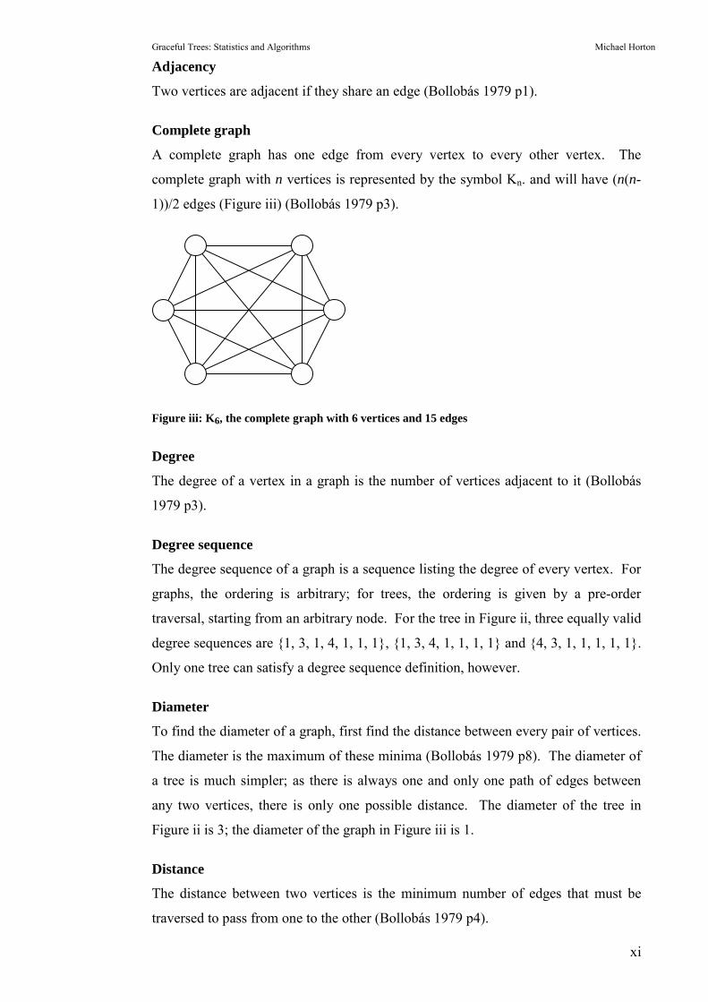
Complete graph
A complete graph has one edge from every vertex to every other vertex. The
complete graph with n vertices is represented by the symbol Kn. and will have (n(n-
1))/2 edges (Figure iii) (Bollobás 1979 p3).
Figure iii: K6, the complete graph with 6 vertices and 15 edges
Degree
The degree of a vertex in a graph is the number of vertices adjacent to it (Bollobás
1979 p3).
Degree sequence
The degree sequence of a graph is a sequence listing the degree of every vertex. For
graphs, the ordering is arbitrary; for trees, the ordering is given by a pre-order
traversal, starting from an arbitrary node. For the tree in Figure ii, three equally valid
degree sequences are {1, 3, 1, 4, 1, 1, 1}, {1, 3, 4, 1, 1, 1, 1} and {4, 3, 1, 1, 1, 1, 1}.
Only one tree can satisfy a degree sequence definition, however.
Diameter
To find the diameter of a graph, first find the distance between every pair of vertices.
The diameter is the maximum of these minima (Bollobás 1979 p8). The diameter of
a tree is much simpler; as there is always one and only one path of edges between
any two vertices, there is only one possible distance. The diameter of the tree in
Figure ii is 3; the diameter of the graph in Figure iii is 1.
Distance
The distance between two vertices is the minimum number of edges that must be
traversed to pass from one to the other (Bollobás 1979 p4).

Graceful Trees: Statistics and Algorithms Michael Horton
xii
Mean
�Mean� without an adjective implies the arithmetic mean (see below.)
Mean, arithmetic
The arithmetic mean of a set of numbers is their sum divided by their count. For
example,
ArithmeticMean([1, 2, 4, 5])
=(1+2+4+5)/4
=12/4
=3
Mean, geometric
The geometric mean of a set of n numbers is the nth root of their product. It is more
commonly calculated by taking the exponent of the arithmetic mean of their natural
logs. The geometric mean is not as vulnerable to high-valued outliers as the
arithmetic mean and may be more appropriate for highly skewed distributions. As an
example,
GeometricMean([1, 2, 4, 5])
=e^(ArithmeticMean([ln(1), ln(2), ln(4), ln(5)]))
=e^(ArithmeticMean(0.000, 0.693, 1.386, 1.609))
=e^(0.922)
=2.515
Isomorphic
Two graphs are isomorphic if they have the same structure � if, by rearranging their
vertex identification, they can be shown to share the same set of edges (Bollobás
1979 p3).
Level
The level of vertices is only meaningful for rooted trees. The level of a vertex is the
distance from it to the root. The level of the root is zero (Wright et al. 1986).
Level sequence
Level sequences are only meaningful for rooted trees. The level sequence is given
by a pre-order traversal of the level of each vertex, starting from the root (Wright et
al. 1986). Trees do not have a single unique level sequence, because the traversal

Graceful Trees: Statistics and Algorithms Michael Horton
xiii
may happen in any order. One possible level sequence for the tree in Figure iv is {0,
1, 2, 2, 2, 1, 1}. Each level sequence does describe a single tree.
Figure iv: A rooted tree, showing the level of each vertex
Lexicographic order
Lexicographic order is a common way to compare sequences; it is used in
dictionaries to order words, which are sequences of letters (Aho & Ullman 1995
p29). For two sequences A and B, A is less than B in lexicographic order if:
1. A is a prefix of B
or
2. For some integer i, A1�i-1≡B1�i-1 and Ai<Bi
Logarithmic scale
Logarithmic scales are a useful way to chart numbers that increase or decrease
exponentially. The chart scale increases exponentially (usually by a multiple of 10)
so that any value that increases exponentially will form a straight line. A
disadvantage is that, because logarithms are only defined for positive numbers, only
positive values can be displayed on a logarithmic scale. The difference between
arithmetic and logarithmic scales is illustrated in Figure v.
0
1 1 1
2 2 2

Graceful Trees: Statistics and Algorithms Michael Horton
xiv
0102030405060708090
100
1 6
x
yy=x!y=3 x̂y=2 x̂y=x
1
10
100
1000
1 6
x
y
y=x!y=3 x̂y=2 x̂y=x
Figure v: Arithmetic and logarithmic scales
Node
A node is another name for a vertex. Within this thesis �node� and �vertex� are used
interchangeably.
Node, Mirrored
All of the work in this thesis is related to trees with labelled nodes. �Mirror Nodes�
are a concept created to describe sets of nodes that do not need to have all possible
labellings tested because they are part of identical structures. For example the three
trees in Figure vi are structurally identical. This means that any algorithm that
looked at all three would be wasting time on the second two.
Figure vi: Example of mirrored nodes – the 2, 3 and 4 can be rearranged at will
Two nodes n1 and n2 are considered mirrored if:
1. The rooted tree with n1 as the root is isomorphic to the rooted tree
with n2 as the root
2. n1 and n2 are adjacent or are adjacent to a common node
�
1
5
2 3 4
6
1
5
4 3 2
6
1
5
2 4 3
6

Graceful Trees: Statistics and Algorithms Michael Horton
1
1 Introduction
A tree with n vertices is �gracefully labelled� if its vertices can be labelled with the
integers [1..n], using each once and only once, such that its edges, when labelled with
the difference between the endpoint vertex labels, are labelled with the integers [1..n-
1], with each number used once and only once. If a tree can be gracefully labelled, it
can be called a �graceful tree� (Rosa 1967).
The �Graceful Tree Conjecture�, or �Ringel-Kötzig Conjecture�, states that all trees
are graceful (Gallian 2000). It has not been proven, although some specialised
classes of tree can be shown to always be graceful (Cahit & Cahit 1975; Pastel &
Raynaud 1978; Hrnciar & Havier 2001; Koh et al. 1980). Computer searches have
also been used to show that all trees with up to 28 vertices are graceful (Aldred &
McKay 1998; Nikoloski et al. 2002). Although searches to finite sizes can never
prove the conjecture true, they may be able to prove it false. They also pose an
intriguing problem in algorithm design, as the exhaustive search demands a very fast
graceful labelling algorithm.
Statistical techniques can also help us estimate trends in graceful labellings, by
showing how the total number of labellings, and the proportion of labellings that are
graceful, change as tree size increases. In particular, statistical trends can suggest if
we can expect that at some large number of vertices a non-graceful tree will be
found.
This thesis describes the development of a new graceful labelling algorithm,
adjustments to improve its running time and its use to prove that all trees with 29
vertices are graceful.
Trends are also found in the statistics of small graceful trees and some future
research directions are proposed.
�

Graceful Trees: Statistics and Algorithms Michael Horton
2
2 Literature Review
2.1 The Graceful Tree Conjecture
A tree with n vertices is said to be gracefully labelled if its vertices are labelled with
the integers [1..n] such that the edges, when labelled with the difference between
their endpoint vertex labels, are uniquely labelled with the integers [1..n-1] (Figure
2-1).
Figure 2-1: An example of a gracefully labelled tree
If a tree can be gracefully labelled, it is called a �graceful tree.� The concept of
graceful labelling of trees and graphs was introduced by Rosa (Rosa 1967) and
named a �β-valuation.� The term �graceful labelling� was invented by Golomb
(Golomb 1972).
The �Graceful Tree Conjecture,� (also known as the �Ringel-Kötzig Conjecture�
(Gallian 2000)) suggests that all trees are graceful. So far, no proof of the truth or
falsity of the conjecture has been found. In the absence of a generic proof, two
approaches have been used in investigating the graceful tree conjecture: proving the
gracefulness of specialised classes of tree, and exhaustively testing trees up to a
specified size for graceful labellings. Both of these approaches are investigated here,
along with some of the related problems in the wider field of graph labelling.
2.2 Approach 1: Classes of graceful tree
Some types of trees have been shown to be always graceful. Many of the proofs that
all trees of a pattern are graceful are also �constructive,� and provide a guaranteed
labelling method for trees that follow that pattern.
1
5 6
2 3
5 4
3
2 1 4

Graceful Trees: Statistics and Algorithms Michael Horton
3
2.2.1 Chains
A chain (or �path�), is the simplest type of tree: a single line of vertices (Figure 2-2).
A chain is a caterpillar (see below) with no legs; chains can always be labelled by
Cahit and Cahit�s caterpillar-labelling algorithm (Cahit & Cahit 1975).
Figure 2-2: The 5-node chain, gracefully labelled by Cahit and Cahit’s algorithm
2.2.2 Caterpillars
A caterpillar is a tree with one long chain of vertices and any number of paths of
length 1 attached to the chain (Figure 2-3). Cahit and Cahit created a constructive
proof that all caterpillars (which they call �string trees�) are graceful (Cahit & Cahit
1975).
Figure 2-3: A caterpillar, gracefully labelled by Cahit and Cahit's algorithm. The upper
horizontal line is the chain section; only paths of length 1 may be attached to it.
2.2.3 m-stars
An m-star has a single root node with any number of paths of length m attached to it
(Figure 2-4). Cahit and Cahit also proved that all m-stars a graceful (Cahit & Cahit
1975).
Figure 2-4: A 2-star, gracefully labelled by Cahit and Cahit's algorithm
9
1
3 6
2 8
5 2
8
5 7
5
1 7
4
3
6
1
14
7
8
6 13
4 113
11 10 9
12
2
13 5
12
10
6
4 2
8
7
9
1
5 3
1 5 2 4 34 3 2 1

Graceful Trees: Statistics and Algorithms Michael Horton
4
2.2.4 Trees with diameter five
The diameter of a graph or tree is the maximum of the shortest paths between its
vertices (Bollobás 1979). Hrnciar and Havier extended the proof for caterpillars to
show that all trees with diameter≤5 are graceful (Hrnciar & Havier 2001).
2.2.5 Olive trees
An olive tree has a root node with k branches attached; the ith branch has length i
(Figure 2-5). Pastel and Raynaud proved that all olive trees are graceful (Pastel &
Raynaud 1978).
Figure 2-5: The k=3 olive tree
2.2.6 Banana trees
A banana tree is constructed by bringing multiple stars together at a single vertex
(Chen et al. 1997) (Figure 2-6). Banana trees have not been proved graceful,
although Bhat-Nayak and Deshmukh have proven the gracefulness of certain classes
of banana tree (Bhat-Nayak & Deshmukh 1996).
Figure 2-6: A banana tree constructed from a 2-star, 3-star and 1-star
Graceful Trees: Statistics and Algorithms Michael Horton
5
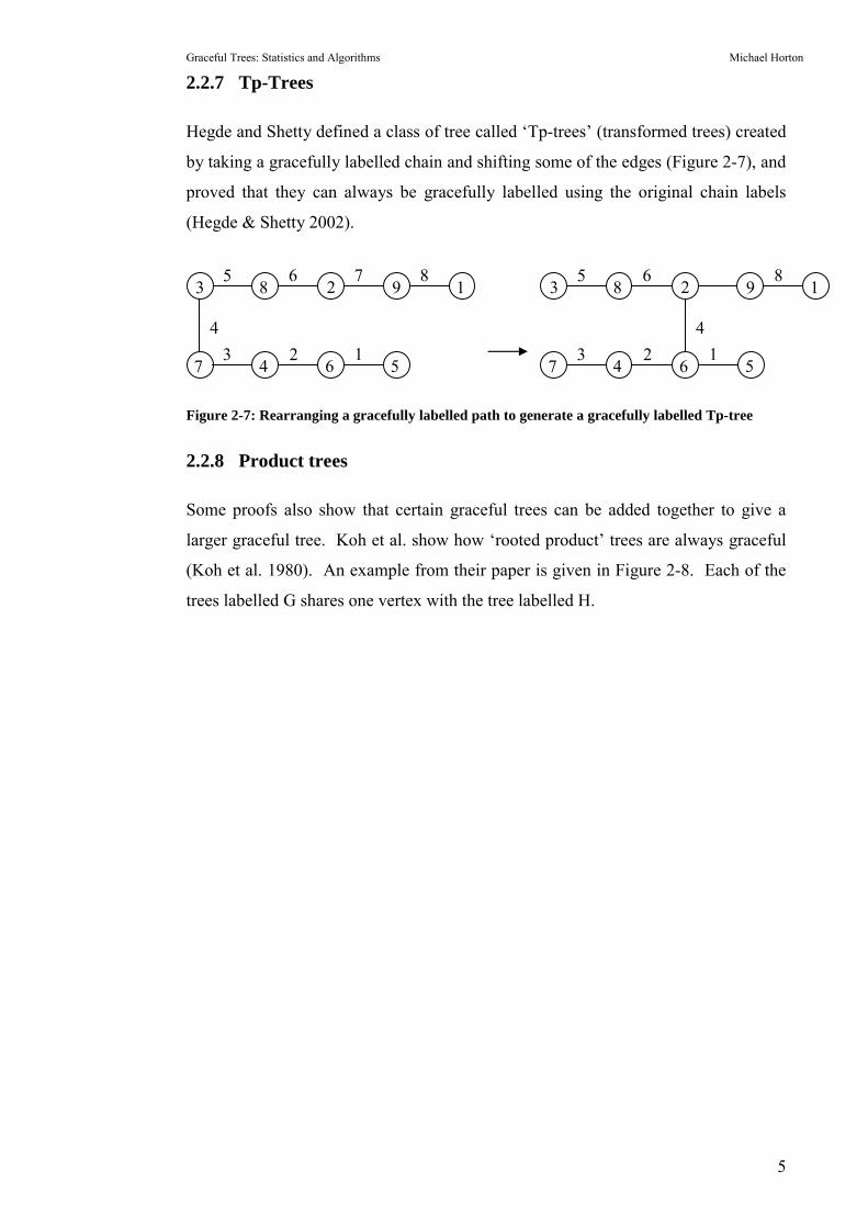
2.2.7 Tp-Trees
Hegde and Shetty defined a class of tree called �Tp-trees� (transformed trees) created
by taking a gracefully labelled chain and shifting some of the edges (Figure 2-7), and
proved that they can always be gracefully labelled using the original chain labels
(Hegde & Shetty 2002).
Figure 2-7: Rearranging a gracefully labelled path to generate a gracefully labelled Tp-tree
2.2.8 Product trees
Some proofs also show that certain graceful trees can be added together to give a
larger graceful tree. Koh et al. show how �rooted product� trees are always graceful
(Koh et al. 1980). An example from their paper is given in Figure 2-8. Each of the
trees labelled G shares one vertex with the tree labelled H.
3
73
5 8
42
6 2
6
4
51
9 18
3
73
5 8
4 2
6 2
6
4
51
9 18 7

Graceful Trees: Statistics and Algorithms Michael Horton
6
Figure 2-8: Example of a graceful product tree
2.3 Approach 2: Exhaustive labelling
The graceful tree conjecture may be wrong. If so, the simplest proof would be to
find a counterexample � a tree that cannot be gracefully labelled. So far, however,
searches have merely found billions of graceful trees, giving additional credence to
the conjecture without formal proof. These currently cover every tree with up to 28
vertices (Aldred & McKay 1998; Nikoloski et al. 2002).
2 3 1
5
4
H
1 62534
3
4
5
1
2
6
1
6
2
5
3
4
5
4
3
1
6
2
G2 G4G3
1
5 6
2
3
4
G1
G5
9
10
11
19
8
12
13
18
14
17
15
16
4 27 526625
23
22
21
7
24
20
1
29 30
2
3
28
G1
G4G3
G2
G5

Graceful Trees: Statistics and Algorithms Michael Horton
7
To run an exhaustive test requires two algorithms: one that finds graceful labellings,
and one that draws every tree of the requested size. Both algorithms must be as
efficient as possible, as the running time limits the size that may be searched to.
2.3.1 Graceful labelling algorithms
2.3.1.1 Exhaustive labelling algorithms
The simplest algorithm to write is to try all n! vertex labellings. This will execute in
O(n!) time, and rapidly becomes impractical as n increases. This algorithm is not
fast enough to test one tree of size 29, to say nothing of every possible tree of size
29. It does have the advantage that it will find not just one graceful labelling but
every possible labelling. This makes it useful for statistical analysis at small sizes.
2.3.1.2 Forward-thinking labelling algorithms
Exhaustive searches can easily find themselves in dead-end states without noticing.
For example, the tree must include edge label n-1. This can only be found between
the vertex labels 1 and n, which therefore must be adjacent to each other. If they
aren�t, the tree cannot possibly be labelled gracefully, and testing labels on the rest of
the tree will merely waste time. Nikoloski et al. found an algorithm that uses a
triangular tableau to identify and ignore cases of this type (Nikoloski et al. 2002).
2.3.1.3 Approximation labelling algorithms
Hill-climbing techniques have also been effective; one was used in Aldred and
McKay�s exhaustive search to n=27 (Aldred & McKay 1998). The general idea is
that any modification to the vertex labels that increases the number of unique edge
labels moves closer to a solution, so is a move up the hill. However, approximate
answers are not sufficient where graceful labellings are concerned. If the hill-
climbing finds itself stuck without reaching n-1 unique edge labels, it must be started
over. The need to restart keeps the hill-climbing technique at exponential efficiency.
To keep this thesis self-contained, Aldred and McKay�s algorithm is described
below.
Graceful and Harmonious alg.
For a given tree T and labelling L of the vertices, let
z(T, L) be the number of distinct edge labels.

Graceful Trees: Statistics and Algorithms Michael Horton
8
For n=|V(T)|, the aim is to find L such that z(T,L)=n-1.
If L is a labelling and v,w∈ V(T), define Sw(L;v, w) to be
the labelling got from L by swapping the labels on v and
w.
Using a parameter M:
1. Start with any labelling of V(T).
2. If z(T,L)=n-1, stop.
3. For each pair {v, w}, replace L by L’=Sw(L;v, w)
if z(T,L’)>z(T, L).
4. If step 3 finishes with L unchanged, replace L by
Sw(L;v, w), where {v, w} is chosen at random from
the set of all {v, w} such that
(a) {v, w} has not been chosen during the most
recent M times this step has been executed.
(b) Sw(L;v, w) is maximal subject to (a).
5. Repeat from step 2.
One part of this algorithm that can be adjusted is the value of M. Aldred and McKay
report that �A value of M=10 seems ok for small trees, but a slightly larger value
seems to be needed for larger trees. The purpose of M is to prevent the algorithm
from repeatedly cycling around within some small set of labellings� (Aldred &
McKay 1998).
2.3.2 Tree construction
2.3.2.1 Constructing all trees
To test every tree with n nodes for a graceful labelling, as Aldred and McKay did,
requires that every tree with n nodes be drawn. Their paper suggests Wright et al.�s
NextTree algorithm (Wright et al. 1986). If NextTree is started with the n-node
chain and called repeatedly, it will draw every unlabelled rootless tree, without
duplicates.
2.3.2.2 Constructing random trees
Another part of working with graceful labelling algorithms is the need to evaluate
their running time over a wide range of tree sizes. For small sizes, they can be tested
on every tree for maximum accuracy, but past the 29-node point, this becomes

Graceful Trees: Statistics and Algorithms Michael Horton
9
unfeasible. The next best alternative is to test the algorithm on an evenly distributed
random sample.
To generate evenly distributed random rootless unlabelled trees we adapted the
algorithm �RANRUT� proposed by Nijenhuis and Wilf (Nijenhuis & Wilf 1978),
which generates random rooted unlabelled trees. In their paper, they give the
algorithm�s FORTRAN source code. For completeness, it is included in appendix A.
2.4 Related problems
As seen above, although the graceful tree conjecture has not been proven, its
investigation has led to many fascinating studies and will probably continue to do so.
Even if a general proof of the conjecture is found, many other problems in the large
field of graph labelling will remain. Gallian has surveyed these in detail (Gallian
2000). Some elements of graph labelling share common ground with graceful trees,
so that proofs or algorithms that are created for one problem may be adaptable to
another. An example is Aldred and McKay�s hill climbing algorithm, which can find
both graceful and harmonious (Figure 2-13) labellings (Aldred & McKay 1998). For
this reason, some of the similar problems in graph labelling are studied here.
2.4.1 Ringel’s Conjecture
The graceful tree conjecture was originally posed as part of an approach to Ringel�s
Conjecture, another problem in graph theory. Ringel�s Conjecture states that, for any
positive n, the complete graph K2n+1 can be decomposed into 2n+1 isomorphic trees
of size n (Ringel 1964) (Figure 2-9).
Figure 2-9: K7 being decomposed into 7 isomorphic trees of size 3

Graceful Trees: Statistics and Algorithms Michael Horton
10
Rosa proved that, if all trees are graceful (that is, if the graceful tree conjecture is
true), Ringel�s Conjecture must be true (Rosa 1967). Ringel�s Conjecture (which is
about graph decomposition) should not be confused with the Ringel-Kötzig
Conjecture (which is another name for the graceful tree conjecture).
2.4.2 Strong graceful labelling
A strong graceful labelling on tree T is defined as one where, for every three
connected vertices x, y and z, either f(x)<f(y)>f(z) or f(x)>f(y)<f(z). Cahit
conjectures that, not only are all trees graceful, but that they can all be strongly
gracefully labelled (Cahit 1994).
2.4.3 Graceful graphs
Graceful labelling of trees may be viewed as a specialised sub-problem of �graceful
graph labelling.� Since graphs frequently have more edges than vertices, a graph
with v vertices and e edges may have its vertices labelled from the set [0..e]. The
edges must then be uniquely labelled with the integers [1..e] (Rosa 1967) (Figure
2-10).
(To be consistent with this, the vertex labels on a graceful tree should be the set [0..n-
1], instead of [1..n]. However, the latter usage has become common and will be used
here.)
Figure 2-10: Example of a gracefully labelled graph
Not all graphs can be gracefully labelled. Several classes of graph have been proven
to be never graceful. Rosa has shown that if every vertex in a graph with e edges has
even degree, and e mod 4 ∈ [1,2], then the graph can never be gracefully labelled
(Rosa 1967). A graph with these properties is in Figure 2-11.
2
0 1
5
4 5
3
2
1

Graceful Trees: Statistics and Algorithms Michael Horton
11
Figure 2-11: A graph that cannot be gracefully labelled
2.4.4 Harmonious graphs and trees
A harmonious labelling of a graph with e edges is the assignment of unique vertex
labels from the set [0..e-1] such that the induced edge labels, where an edge label is
the sum of its end vertex labels, are distinct (Graham & Sloane 1980) (Figure 2-12).
Figure 2-12: A harmoniously labelled graph
Since a tree with e edges has (e+1) vertices, the definition of a harmonious tree
permits one of the vertex labels to be repeated. Graham and Sloane have conjectured
that all trees are harmonious (Graham & Sloane 1980) (Figure 2-13).
Figure 2-13: A harmoniously labelled tree
Many of the proofs and algorithms that are used to approach the graceful tree
conjecture also work on harmonious trees. Aldred and McKay also applied their hill-
climbing labelling algorithm to harmonious trees and found harmonious labellings
for all trees with up to 26 vertices (Aldred & McKay 1998).
0
2 3
3 4
3 2
1
4 5 1
2
0 1
3
4 3
5
2
1

Graceful Trees: Statistics and Algorithms Michael Horton
12
2.4.5 Cordial graphs and trees
A simpler form of labelling is suggested by Cahit (Cahit 1987). All vertices are
labelled from the set [0,1], and edges are labelled as the difference of end vertices.
The labelling is cordial if the difference between (number of vertices labelled 0) and
(number of vertices labelled 1) is at most 1, and the difference between (number of
edges labelled 0) and (number of edges labelled 1) is at most 1 (Figure 2-14, Figure
2-15).
Figure 2-14: A cordially labelled graph
Figure 2-15: A cordially labelled tree
Cahit later proved that all trees are cordial, and also determined some properties that
show whether a graph is cordial (Cahit 1990). This includes proof that the n-node
complete graph Kn can only be cordially labelled when n≤3 (Figure 2-16).
Figure 2-16: K4: A graph that cannot be cordially labelled
1
0 1
0 0
0 1
0
1 1 1
1
0 0
1
1 1
0
1
0

Graceful Trees: Statistics and Algorithms Michael Horton
13
2.5 Summary
The graceful tree conjecture has yet to be proven. Specialised proofs show that
limited types of trees are graceful for all sizes, while exhaustive searches show that
limited sizes of tree are graceful for all types.
The exhaustive search approach has also given rise to the field of graceful labelling
algorithms, which are an interesting problem in algorithm design.
�

Graceful Trees: Statistics and Algorithms Michael Horton
14
3 Methods
3.1 Introduction
In order to carry out an exhaustive labelling of every tree with 29 nodes, it is
necessary to actually draw the trees. Sometimes, however, drawing every tree is
impractical � when analysing an algorithm�s running time on 40-node trees, for
example. The algorithm may instead be tested on a random sample of 40-node trees.
3.2 Drawing every size n tree
Several parts of this investigation required that every n-node tree be drawn. In
particular, all trees with 29 nodes were tested to see if they admitted a graceful
labelling. There are 5,469,566,585 such trees (Otter 1948); to generate all of them in
reasonable time is not a trivial exercise. NextTree, an efficient algorithm that draws
all trees of size n with constant time per tree and O(n) space (Wright et al. 1986) was
chosen. The pseudocode of NextTree is given in appendix A.
3.2.1 Encoding the trees
This algorithm uses a tree encoding called the primary canonical level sequence.
This extends the notion of a canonical level sequence, which is discussed by Beyer
and Hedetniemi (Beyer & Hedetniemi 1980) to draw all unique n�node rooted trees.
The canonical level sequence of a tree is the distance of every node from the root,
sequenced by a pre-order traversal that visits subtrees in nonincreasing lexicographic
order. The primary canonical level sequence is a canonical sequence rooted at the
centre of the tree. For trees with two centre nodes, the root with fewer nodes on its
side of the centre is chosen. If both potential roots have the same number of nodes,
the root that generates a lexicographically smaller canonical level sequence is
chosen. If the canonical level sequences are identical, both roots would generate the
same primary canonical level sequence, so choice of root is irrelevant.
3.2.2 Generating the trees
If Wright et al.�s �NextTree� algorithm is given the primary canonical level sequence
of any tree, it will generate the primary canonical level sequence of a new tree. If it
is started with the size n chain, it will generate the primary canonical level sequence

Graceful Trees: Statistics and Algorithms Michael Horton
15
of every unique n-node rootless tree, finishing with the size n 1-star. An example of
the trees it draws, in order, is given in Figure 3-1.
Figure 3-1: The primary canonical level sequences and resulting trees drawn by successive calls
to NextTree for n=6
The NextTree algorithm generated all 5,469,566,585 trees with 29 nodes within 10
minutes on a 2.4 GhZ Pentium IV. Testing every tree for a graceful labelling would
take a little longer. Specifically, it took 58 days. The running time may therefore be
considered negligible compared to the labelling time.
3.3 Drawing random size n trees
Some of the algorithm runtime analysis had to be run without a full set of trees.
Instead, it was tested on a random sample, which should be as evenly distributed as
Tree 1
Level sequence=1 2 3 3 2 3
Tree 0
Level sequence=1 2 3 4 2 3
Tree 2
Level sequence=1 2 3 3 2 2
Tree 3
Level sequence=1 2 3 2 3 2
Tree 4
Level sequence=1 2 3 2 2 2
Tree 5
Level sequence=1 2 2 2 2 2

Graceful Trees: Statistics and Algorithms Michael Horton
16
possible � if the random sample is biased in favour of some pattern of trees, the
running time will be inaccurate.
(The computers used in this research were not able to generate truly random
numbers, so the algorithms as implemented could only generate pseudorandom
trees.)
3.3.1 Simple random tree construction
Constructing random trees is quite simple if the problem of distribution is ignored.
For the initial tests, the following algorithm was used:
Algorithm ConstructRandomTree
Input: Random number seed, size
Output: A random tree of appropriate size
Variables: parent, an array[0..size-1] of integer. This
stores the parent of each node. A parent of -1 indicates
that the node has no parent (it is the root.)
parent[0]<- -1
For every node i from 1 to size-1
parent[i]<-random(0..i-1)
This may generate every unlabelled tree with size nodes, but the distribution will not
be even.
3.3.2 Evenly distributed random tree construction
3.3.2.1 Random rooted unlabelled trees
For more robust results, the RANRUT algorithm written by Nijenhuis and Wilf
(Nijenhuis & Wilf 1978) was chosen. The complete FORTRAN source written by
Nijenhuis and Wilf is included in appendix A. RANRUT generates an even
distribution of random unlabelled rooted trees.
3.3.2.2 Random rootless unlabelled trees
For this project, RANRUT was adapted to only accept trees where the root had the
lexicographically greatest degree sequence. If multiple nodes had the same degree
sequence, the tree was only used if a random number in the range 0..(number of

Graceful Trees: Statistics and Algorithms Michael Horton
17
nodes with the equal greatest degree sequence-1) returned zero. These changes
meant that the algorithm generated an even distribution of random unlabelled
rootless trees as required. This adaption worked, although it was quite slow (Table
3-1).
Tree size Mean drawing time (s) 4 0.0007308 0.004762
12 0.01812916 0.04553120 0.08825824 0.03094528 0.01257032 0.016297
Table 3-1: RANRUT mean running time per tree, for 256 trees of each size
The random rootless tree drawing algorithm was still capable of generating trees for
run time analysis at sizes that were too large for exhaustive testing with NextTree.
�

Graceful Trees: Statistics and Algorithms Michael Horton
18
4 The edge search algorithm
4.1 Introduction
The simplest approach to writing a graceful labelling algorithm is to concentrate
upon fitting node labels into the tree. However, another possibility is to concentrate
on fitting the edge labels, while making sure that no invalid node labels are used.
This possibility inspired the edge-based depth-first search graceful labelling
algorithm described here.
The edge search algorithm applies the edge labels in sequence, starting with edge
label n-1, then putting edge n-2 adjacent to that, then n-3 adjacent to one of the
existing edges, continuing until edge label 2 and edge label 1 are applied. Edge
search assumes that a graceful labelling exists where every edge smaller that n-1 can
be fitted adjacent to an edge with a greater label. This leads to a conjecture that is
discussed in section 4.5.
Edge search has some similarities with an unpublished algorithm by Suraweera and
Anderson (Suraweera & Anderson 2002) which analyses the degree sequence and
fits edges around it.
The data found for the running time analyses in this chapter are listed in appendix B.
4.2 The basic algorithm (EdgeSearchBasic)
Although it was expanded in several ways, the edge search algorithm started like
this:
Algorithm EdgeSearchBasic
Input:
T, a rootless tree that stores adjacency lists for every
node.
Output:
A graceful labelling for the input tree.
Variables:
Graceful Trees: Statistics and Algorithms Michael Horton
19
Size, the size of the tree
Possible, an array of Booleans storing which nodes are
candidates for edge labelling
Procedure search
For every possible starting node from 0 to size-1
Set all nodes impossible
Set the label of the starting node to 1
Record that all nodes adjacent to the starting
node are possible
FindEdge(Size-1)
End for
End procedure
Procedure FindEdge
Input:
EdgeLabel, the edge currently being searched for
T, a rootless tree with a spanning tree of edge labels
from Size to EdgeLabel+1
Output:
A graceful labelling of T, if one was found.
Variables:
PossibleNode, a node found on the possible list
PreviousNode, the labelled node above PossibleNode
LowLabel & HighLabel, the two possible node labels that
could be used to achieve EdgeLabel on the edge between
PreviousNode and PossibleNode
TestLabel, the node label decided upon
If EdgeLabel=0 then
Record labelling found
Else
For every node marked possible

Graceful Trees: Statistics and Algorithms Michael Horton
20
PossibleNode←the possible node PreviousNode←the node above PossibleNode LowLabel←PreviousNode’s label-EdgeLabel HighLabel←PreviousNode’s label+EdgeLabel
If LowLabel or HighLabel are within the
range 1..size and have not already been
used then
TestLabel←the potential label NodeLabel[PossibleNode]<TestLabel
Record that PossibleNode now has
label TestLabel
Record that the node label TestLabel
has been used
Set PossibleNode impossible
Set all nodes adjacent to
PossibleNode possible
FindEdge(EdgeLabel-1)
Restore the state before this
labelling was tried (set all adjacent
nodes impossible, set PossibleNode
back to possible and record that node
label TestLabel may be used again.)
End if
End for
End else
End procedure
4.3 Example
Here, the algorithm is shown running on a 5-node tree. The thick lines indicate the
section of the tree that has been labelled. The �P� labels show which nodes are
marked �possible� at each stage of the algorithm.

Graceful Trees: Statistics and Algorithms Michael Horton
21
Figure 4-1: The edge search starts by testing node label 1 on the first node. All nodes adjacent
to the labelled node are marked possible.
Figure 4-2: The first edge label to be considered is 4. It is tested on the first possible node. Since
the node above the possible node is labelled 1, a node label of -3 or 5 is required to achieve this.
Only 5 lies within the bounds of the possible node labels, so it is applied.
Figure 4-3: Whenever a possible node is labelled, all unlabelled adjacent nodes are marked
possible.
4 3
1
5 4 P
P
4
1
5 P P
1
P P P

Graceful Trees: Statistics and Algorithms Michael Horton
22
Figure 4-4: The initial search gets this far but can’t find any way to obtain edge label 1, so it
backtracks.
Figure 4-5: The next recursion tries edge label 2 on the bottom node but has no better luck.
Figure 4-6: Since edge label 3 to the centre node failed, it’s tried to the right-hand node.
Figure 4-7: This time, edge labels 2 and 1 follow easily and a graceful labelling is recorded.
1
4 3 2
1
5 3 4
2
4 3
1
5 P 4
2
4 3
1
5 4 P
2
4 2 3
1
5 4 3
P

Graceful Trees: Statistics and Algorithms Michael Horton
23
4.3.1 Correctness
The two requirements of a graceful labelling are that the nodes be uniquely labelled
with integers [1..n] and that the edges be uniquely labelled with the integers [1..n-1].
The FindEdge procedure labels edges starting with n-1 and moving downwards. If
the EdgeLabel argument to FindEdge reaches 0, it must have found somewhere to fit
every edge from n-1 down to 1, using every edge once and only once. Therefore, the
edge labelling requirement must be satisfied.
The FindEdge procedure records whether each node label has been used. It never
uses a node label outside the range 1..n and cannot reuse node labels. It starts with
one node labelled and no edges labelled, and every edge label requires one new node
label. Therefore, after the n-1 edges have been labelled, the n nodes will be labelled
with the unique integers [1..n].
Since both requirements are satisfied, any labelling reported by the basic edge search
algorithm will be graceful.
4.3.2 Termination
The edge search algorithm considers starting points and next node options in
increasing order, it will never reconsider a labelling that it has previously reached.
Since there are a finite number of possible labellings, the basic edge search algorithm
will always terminate in finite time.
Unfortunately, termination may still take a very long time; just how long is discussed
just below in section 4.3.3.
4.3.3 Run-time analysis
4.3.3.1 Theory
The running time for most algorithms is measured in two ways � in seconds, or in
operations. Running time in seconds is easier to understand, but depends upon
computer speed (all running times given are for a 2.4 GhZ Pentium IV.) Running
time is also often either too small to measure or too large to use for all algorithms.
Operations can be hard to count. In the case of the edge search algorithm, there is
one simple measure: the number of calls to the FindEdge procedure. Almost all

Graceful Trees: Statistics and Algorithms Michael Horton
24
labelling time is spent in FindEdge, so it is a useful measure. It will not be perfect
because the running time of each call is not constant � it will change depending upon
the number of nodes considered possible.
In tests, once the running time became measurable, both average and worst-case
running time were closely correlated with average and worst-case calls to FindEdge
(Figure 4-8 and Figure 4-9).
y = 1E-07xR2 = 0.9996
0.0001
0.001
0.01
0.1
11 10 100 1000 10000 100000 1000000
Mean calls to FindEdge
Mea
n tim
e (s
) Time against calls toFindEdge
Linear (Time againstcalls to FindEdge)
Figure 4-8: Chart showing how mean calls to FindEdge is closely correlated to mean running
time. Both scales are logarithmic.

Graceful Trees: Statistics and Algorithms Michael Horton
25
y = 1E-07xR2 = 0.9999
0.01
0.1
1
10
100
1000
1 10 100 1000 10000 100000 1000000 10000000 100000000
1E+09 1E+10
Worst calls to FindEdge
Wor
st ti
me
(s)
Time against calls toFindEdge
Linear (Time againstcalls to FindEdge)
Figure 4-9: Chart showing how worst-case calls to FindEdge is closely correlated to worst-case
running time. Both scales are logarithmic.
4.3.3.2 Results
Every tree on 1 to 15 nodes was gracefully labelled with EdgeSearchBasic. Running
time in seconds and number of calls to the FindEdge procedure were measured.
Both the mean and worst-case running time for the basic edge search increase very
rapidly. Note that the worst-case time (Figure 4-10) is 5000 times worse than the
average (Figure 4-11).
0
50
100
150
200
250
0 2 4 6 8 10 12 14 16
Tree size
Tim
e (s
)
Figure 4-10: Basic edge search algorithm worst-case running time (arithmetic scale)

Graceful Trees: Statistics and Algorithms Michael Horton
26
0
0.005
0.01
0.015
0.02
0.025
0.03
0.035
0.04
0.045
0.05
0 2 4 6 8 10 12 14 16
Tree size
Tim
e (s
)
Figure 4-11: Basic edge search algorithm mean running time (arithmetic scale)
These are easier to see on a logarithmic scale (Figure 4-12).
0.0001
0.001
0.01
0.1
1
10
100
1000
0 2 4 6 8 10 12 14 16
Tree size
Tim
e (s
)
Worst time (s)Seconds/tree
Figure 4-12: Basic edge search algorithm worst-case and mean running time (logarithmic scale)
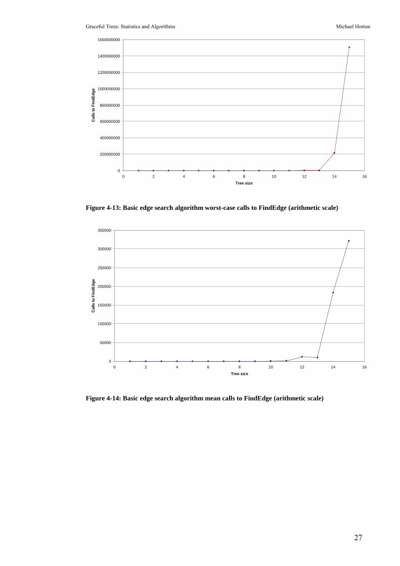
The count of calls to the FindEdge function follow the same trend as time (Figure
4-13, Figure 4-14 and Figure 4-15).
Graceful Trees: Statistics and Algorithms Michael Horton
27
0
200000000
400000000
600000000
800000000
1000000000
1200000000
1400000000
1600000000
0 2 4 6 8 10 12 14 16
Tree size
Cal
ls to
Fin
dEdg
e
Figure 4-13: Basic edge search algorithm worst-case calls to FindEdge (arithmetic scale)
0
50000
100000
150000
200000
250000
300000
350000
0 2 4 6 8 10 12 14 16
Tree size
Cal
ls to
Fin
dEdg
e
Figure 4-14: Basic edge search algorithm mean calls to FindEdge (arithmetic scale)

Graceful Trees: Statistics and Algorithms Michael Horton
28
1
10
100
1000
10000
100000
1000000
10000000
100000000
1000000000
10000000000
0 2 4 6 8 10 12 14 16
Tree size
Cal
ls to
Fin
dEdg
e
Worst calls to FindEdgeMean calls to FindEdge
Figure 4-15: Basic edge search worst-case and mean calls to FindEdge (logarithmic scale)
The basic edge search algorithm would take far too long if it tried to label most 29-
node trees. However, this form was still far faster than the basic factorial-time
search used in chapter 6. Several adjustments were then made to improve the
running time.
4.4 Extensions
4.4.1 Restarting after excess time
The most serious problem with the edge search was its occasional tendency to get
into time-consuming dead ends. For some trees, no labelling exists for certain
starting nodes, yet the edge search spends a long time trying out labellings. The
simplest fix was to record the time when the first node was labelled, and calculate
how long the search had run. After excess time (0.2-1.0 seconds was found
sufficient on the hardware used), a new starting node was chosen at random.
The modified algorithm did find labellings faster, but was implementation-
dependent. It is also no longer guaranteed to terminate � if a non-graceful tree exists,
it will continue testing it forever.

Graceful Trees: Statistics and Algorithms Michael Horton
29
4.4.2 Restarting after excess failures (EdgeSearchRestart)
There were occasions when the �FindEdge� procedure could not find any way to
extend the partial tree. This could be recognised and counted � if the edge requested
couldn�t fit anywhere, the �failure count� was incremented. If the failure count
exceeded a preset �failure tolerance�, the search was restarted with a new node. If all
n starting nodes were tested and no labelling resulted, the search was restarted with
two changes:
1. The adjacency list of every node was scrambled. Since nodes were
added to the �possible� list in their order from the adjacency list, this
meant the �possible� list would have a different ordering.
2. The failure tolerance was increased. This gave more chances to find a
correct labelling, at the expense of more time spent searching failed
labellings.
Choosing the failure tolerance starting point and increment required some
adjustment. Initially, it started at 1 and was doubled after a restart.
Observation showed that a graceful labelling was often found after approximately n2
failures, so the starting tolerance was set to n2. Initially the increment was n. This
worked well on the average case, but was very poor in the worst case. At size 28,
one tree still suffered 2.95*107 failures after selecting the correct starting node.
After observing cases like this, the increment was changed back to doubling the
failure tolerance.
Failure-based restart, with failure tolerance starting at n2 and doubling after try all n
starting points, worked well. It does still suffer from the same problem as the time-
based restart � it is not guaranteed to terminate if a non-graceful tree exists. If the
tree is graceful, the failure tolerance will eventually climb high enough that every
possible labelling will be tested.
The proof of correctness in section 4.3.1 still holds, so if the algorithm does
terminate, the labelling it reports will be graceful.
The basic algorithm measurements became very time-consuming at all 15-node trees;
this algorithm was tested on all trees with up to 22 nodes. The worst-case running

Graceful Trees: Statistics and Algorithms Michael Horton
30
time still climbs rapidly (Figure 4-16 and Figure 4-19), but was far better in constant
terms than the basic algorithm, and the mean is much shallower (Figure 4-17 and
Figure 4-19). This is also apparent on the logarithmic scale (Figure 4-18 and Figure
4-21).
0
5
10
15
20
25
30
35
0 5 10 15 20 25
Tree size
Tim
e (s
)
Figure 4-16: EdgeSearchRestart worst-case running time (arithmetic scale)
0.00E+00
5.00E-05
1.00E-04
1.50E-04
2.00E-04
2.50E-04
3.00E-04
3.50E-04
4.00E-04
0 5 10 15 20 25
Tree size
Tim
e (s
)
Figure 4-17: EdgeSearchRestart mean running time (arithmetic scale)

Graceful Trees: Statistics and Algorithms Michael Horton
31
0.00001
0.0001
0.001
0.01
0.1
1
10
100
0 5 10 15 20 25
Tree size
Tim
e (s
)
Worst time (s)Mean time (s)
Figure 4-18: EdgeSearchRestart worst-case and mean running time (logarithmic scale)
0
20000000
40000000
60000000
80000000
100000000
120000000
140000000
160000000
180000000
0 5 10 15 20 25
Tree size
Cal
ls to
Fin
dEdg
e
Figure 4-19: EdgeSearchRestart worst-case calls to FindEdge (arithmetic scale)
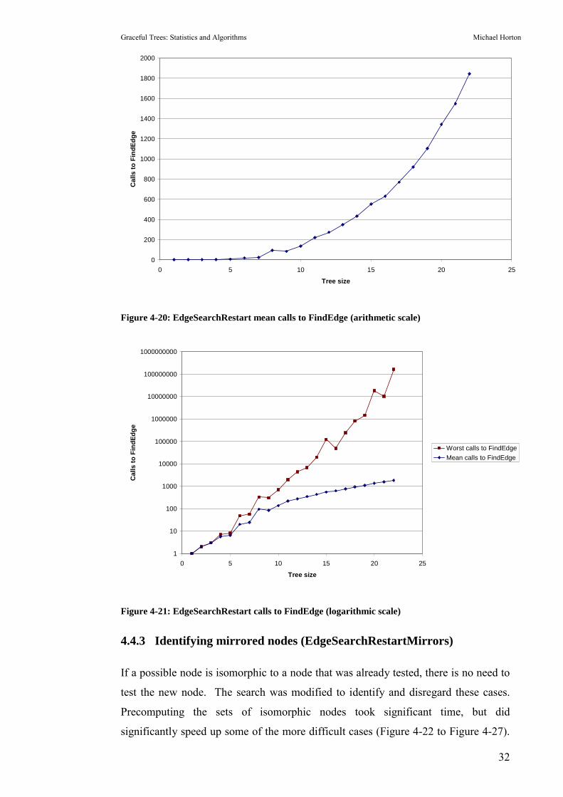
Graceful Trees: Statistics and Algorithms Michael Horton
32
0
200
400
600
800
1000
1200
1400
1600
1800
2000
0 5 10 15 20 25
Tree size
Cal
ls to
Fin
dEdg
e
Figure 4-20: EdgeSearchRestart mean calls to FindEdge (arithmetic scale)
1
10
100
1000
10000
100000
1000000
10000000
100000000
1000000000
0 5 10 15 20 25
Tree size
Cal
ls to
Fin
dEdg
e
Worst calls to FindEdgeMean calls to FindEdge
Figure 4-21: EdgeSearchRestart calls to FindEdge (logarithmic scale)
4.4.3 Identifying mirrored nodes (EdgeSearchRestartMirrors)
If a possible node is isomorphic to a node that was already tested, there is no need to
test the new node. The search was modified to identify and disregard these cases.
Precomputing the sets of isomorphic nodes took significant time, but did
significantly speed up some of the more difficult cases (Figure 4-22 to Figure 4-27).

Graceful Trees: Statistics and Algorithms Michael Horton
33
The mean running time is now very shallow (Figure 4-23), suggesting that the
algorithm is very efficient for most trees. The worst-case efficiency remains
exponential (Figure 4-22 and Figure 4-24), although it is very good in constant terms.
0
0.2
0.4
0.6
0.8
1
1.2
1.4
1.6
0 5 10 15 20 25
Tree size
Tim
e (s
)
Figure 4-22: EdgeSearchRestartMirrors worst-case running time (arithmetic scale)
Mean time (s)
0
0.0001
0.0002
0.0003
0.0004
0.0005
0.0006
0 5 10 15 20 25 30
Tree size
Tim
e (s
)
Figure 4-23: EdgeSearchRestartMirrors mean running time (arithmetic scale)

Graceful Trees: Statistics and Algorithms Michael Horton
34
0.0001
0.001
0.01
0.1
1
10
0 5 10 15 20 25 30
Tree size
Tim
e (s
)
Worst time (s)Mean time (s)
Figure 4-24: EdgeSearchRestartMirrors worst-case and mean running time (logarithmic scale)
0
1000000
2000000
3000000
4000000
5000000
6000000
0 5 10 15 20 25 30
Tree size
Cal
ls to
Fin
dEdg
e
Figure 4-25: EdgeSearchRestartMirrors worst-case calls to FindEdge (arithmetic scale)

Graceful Trees: Statistics and Algorithms Michael Horton
35
0
50
100
150
200
250
300
350
400
450
500
0 5 10 15 20 25 30
Tree size
Cal
ls to
Fin
dEdg
e
Figure 4-26: EdgeSearchRestartMirrors mean calls to FindEdge (arithmetic scale)
1
10
100
1000
10000
100000
1000000
10000000
0 5 10 15 20 25 30
Tree size
Cal
ls to
Fin
dEdg
e
Worst calls to FindEdgeMean calls to FindEdge
Figure 4-27: EdgeSearchRestartMirrors worst-case and mean calls to FindEdge (logarithmic
scale)
EdgeSearchRestartMirrors was also tested on 4096 trees in each size from 4 to 60.
For all its improvements, its mean running time and calls to FindEdge eventually
climb exponentially (Figure 4-29, Figure 4-30, Figure 4-32 and Figure 4-33). The
worst cases found follow much the same trend, but higher (Figure 4-28 and Figure
4-31). Note that these are just the worst cases found out of the 4096 random trees �
they are not the absolute worst case at each size.

Graceful Trees: Statistics and Algorithms Michael Horton
36
0
500
1000
1500
2000
2500
3000
0 10 20 30 40 50 60 70
Tree size
Wor
st-c
ase
runn
ing
time
(s)
Figure 4-28: EdgeSearchRestartMirrors worst-case running time for random trees (arithmetic
scale)
0.00E+00
5.00E-01
1.00E+00
1.50E+00
2.00E+00
2.50E+00
0 10 20 30 40 50 60 70
Tree size
Mea
n ru
nnin
g tim
e (s
)
Figure 4-29: EdgeSearchRestartMirrors mean running time for random trees (arithmetic scale)

Graceful Trees: Statistics and Algorithms Michael Horton
37
1.00E-05
1.00E-04
1.00E-03
1.00E-02
1.00E-01
1.00E+00
1.00E+01
1.00E+02
1.00E+03
1.00E+04
0 10 20 30 40 50 60 70
Tree size
Run
ning
tim
e (s
)
Mean time (s) Worst time (s)
Figure 4-30: EdgeSearchRestartMirrors worst-case and mean running time for random trees
(logarithmic scale)
0
1000000000
2000000000
3000000000
4000000000
5000000000
6000000000
7000000000
0 10 20 30 40 50 60 70
Tree size
Wor
st c
alls
to F
indE
dge
Figure 4-31: EdgeSearchRestartMirrors worst-case calls to FindEdge for random trees
(arithmetic scale)
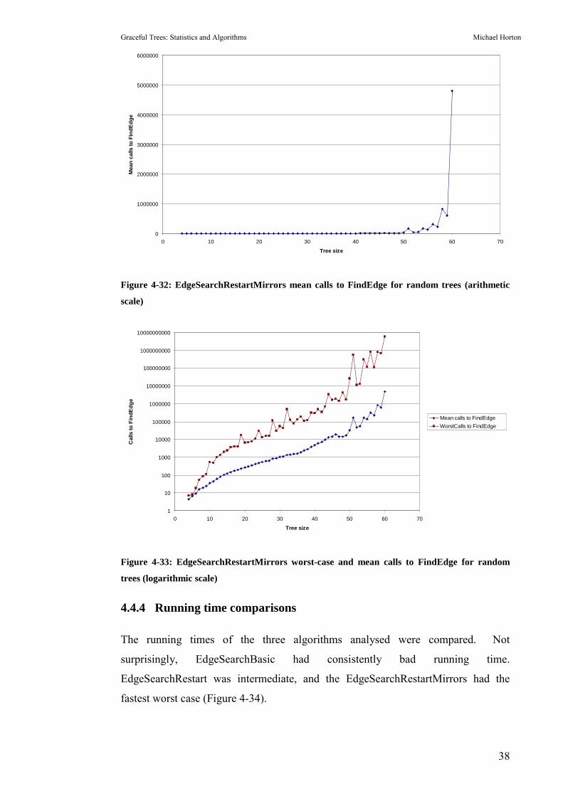
Graceful Trees: Statistics and Algorithms Michael Horton
38
0
1000000
2000000
3000000
4000000
5000000
6000000
0 10 20 30 40 50 60 70
Tree size
Mea
n ca
lls to
Fin
dEdg
e
Figure 4-32: EdgeSearchRestartMirrors mean calls to FindEdge for random trees (arithmetic
scale)
1
10
100
1000
10000
100000
1000000
10000000
100000000
1000000000
10000000000
0 10 20 30 40 50 60 70
Tree size
Cal
ls to
Fin
dEdg
e
Mean calls to FindEdge WorstCalls to FindEdge
Figure 4-33: EdgeSearchRestartMirrors worst-case and mean calls to FindEdge for random
trees (logarithmic scale)
4.4.4 Running time comparisons
The running times of the three algorithms analysed were compared. Not
surprisingly, EdgeSearchBasic had consistently bad running time.
EdgeSearchRestart was intermediate, and the EdgeSearchRestartMirrors had the
fastest worst case (Figure 4-34).
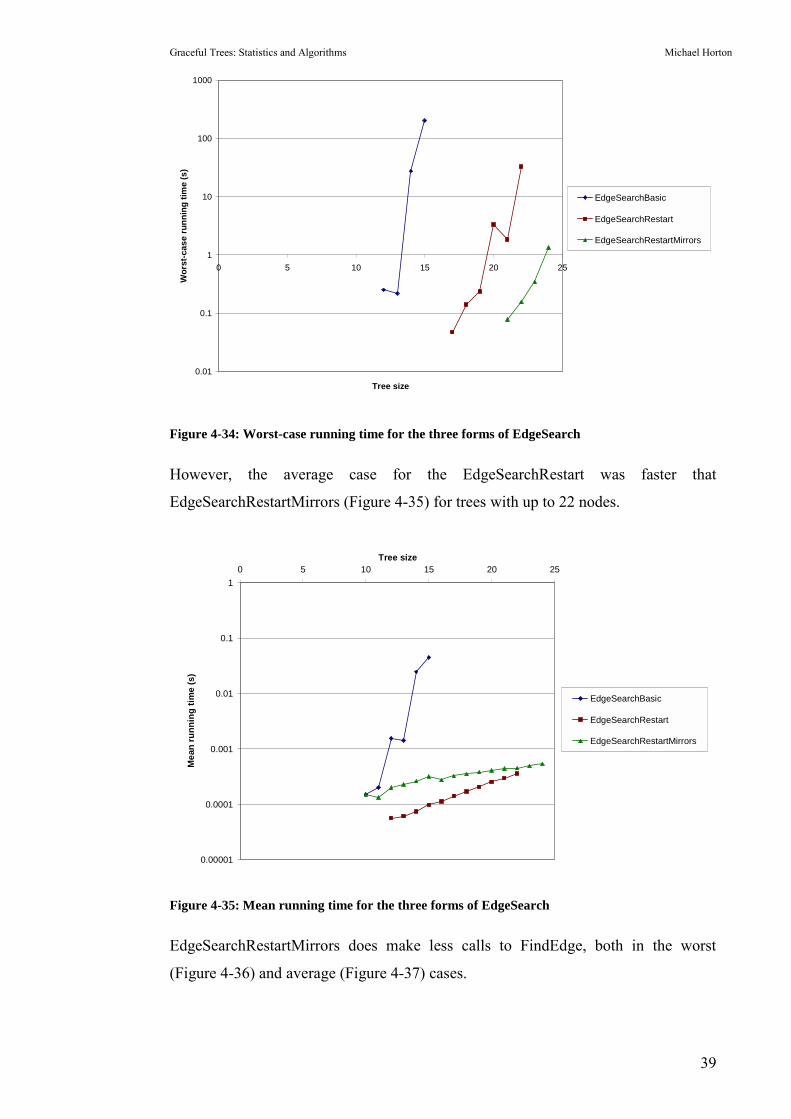
Graceful Trees: Statistics and Algorithms Michael Horton
39
0.01
0.1
1
10
100
1000
0 5 10 15 20 25
Tree size
Wor
st-c
ase
runn
ing
time
(s)
EdgeSearchBasic
EdgeSearchRestart
EdgeSearchRestartMirrors
Figure 4-34: Worst-case running time for the three forms of EdgeSearch
However, the average case for the EdgeSearchRestart was faster that
EdgeSearchRestartMirrors (Figure 4-35) for trees with up to 22 nodes.
0.00001
0.0001
0.001
0.01
0.1
10 5 10 15 20 25
Tree size
Mea
n ru
nnin
g tim
e (s
)
EdgeSearchBasic
EdgeSearchRestart
EdgeSearchRestartMirrors
Figure 4-35: Mean running time for the three forms of EdgeSearch
EdgeSearchRestartMirrors does make less calls to FindEdge, both in the worst
(Figure 4-36) and average (Figure 4-37) cases.

Graceful Trees: Statistics and Algorithms Michael Horton
40
1
10
100
1000
10000
100000
1000000
10000000
100000000
1000000000
10000000000
0 5 10 15 20 25
Tree size
Wor
st c
alls
to F
indE
dge
EdgeSearchBasic
EdgeSearchRestart
EdgeSearchRestartMirrors
Figure 4-36: Worst-case calls to FindEdge for the three forms of EdgeSearch
1
10
100
1000
10000
100000
1000000
0 5 10 15 20 25
Tree size
Mea
n ca
lls to
Fin
dEdg
e
EdgeSearchBasic
EdgeSearchRestart
EdgeSearchRestartMirrors
Figure 4-37: Mean calls to FindEdge for the three forms of EdgeSearch
Since EdgeSearchRestartMirrors makes less calls to FindEdge but takes longer than
EdgeSearchRestart, the time lost by EdgeSearchRestartMirrors must be during its
additional preparation to identify mirrored nodes. This appears worthwhile when
labelling difficult trees, but not when labelling simple ones. The slope of the
EdgeSearchRestart mean running time is steeper than that of

Graceful Trees: Statistics and Algorithms Michael Horton
41
EdgeSearchRestartMirrors (Figure 4-35), suggesting that EdgeSearchRestartMirrors
will be faster on average at larger tree sizes.
4.5 The edge search conjecture
The edge search algorithm does not consider every possible node labelling, due to its
requirement that each edge be applied adjacent to previous edges. At every stage,
the labelled edges will form a subtree. This means it could never generate the
following graceful labelling in Figure 4-38, because edge label 2 is not adjacent to
edge labels 3, 4 or 5.
Figure 4-38: Example of a graceful labelling not covered by the edge search conjecture
Despite this, the edge search always appears to generate a graceful labelling. This
leads us to conjecture that all trees admit a graceful labelling where every edge label
other than n-1 is adjacent to one edge of greater label.
This form of graceful labelling is already known; Cahit�s algorithm for labelling
caterpillars will always generate a labelling of this type (Cahit & Cahit 1975).
However, it has not been previously suggested that all trees admit this form of
graceful labelling.
4.6 The final algorithm
This algorithm features both the changes found useful in EdgeSearchRestartMirrors.
Specifically:
1. FindEdge detects when it can�t find any edge that will fit the
requested edge label. This requires the new variable EdgeFound.
2. FindEdge records the number of times that it can�t find any edge that
will fit. This requires the new variables FailureCount and GivenUp.
3. If the FailureCount exceeds the failure tolerance, the whole search is
restarted from another node. This requires the new variable
FailureTolerance. After all nodes have been tested, FailureTolerance
2 4 3 6 1 2 1 3 5 4 5

Graceful Trees: Statistics and Algorithms Michael Horton
42
is increased and the adjacency lists are scrambled, using the
ScrambleNext procedure.
4. Starting nodes are not used if they are identical to nodes that have
already been tested � that is, if the tree, rooted from the potential
starting node, is isomorphic to the tree when rooted from an earlier
node. The IdenticalNode array stores these.
5. FindNext doesn�t try fitting to nodes that are mirrors (p. xiv) of nodes
that have already been tested. It looks up the sets that nodes belong to
in the NodeSet array.
It is important to note the IdenticalNode and NodeSet arrays do not use the same
information, as Figure 4-39 explains.
Figure 4-39: This shows the difference between IdenticalNode and NodeSet. All nodes marked
with an ‘I’ are identical for the purposes of starting nodes, but only those marked with an ‘S’
are part of the same set when FindEdge is running.
Algorithm EdgeSearchRestartMirrors
Input:
T, a rootless tree that stores adjacency lists for every
node
Output:
A graceful labelling for the input tree
Variables:
Size, the size of the tree
Possible, an array of Booleans storing which nodes are
candidates for edge labelling
SI ISI SI I I

Graceful Trees: Statistics and Algorithms Michael Horton
43
GivenUp, a boolean tracking if the labelling should be
restarted from 1
FailureCount, an integer storing the number of times that
FindEdge has found no ways to fit an edge label
FailureTolerance, an integer storing how large
FailureCount can get before restarting
NodeSet, an array of integers storing which set of
mirrored nodes each node belongs to (-1 if there are no
matching nodes)
IdenticalNode, an array of integers storing the index of
the first lower numbered node identical to this one (-1
if there isn’t one)
Procedure search
FailureTolerance←Size2
FailureCount←0 Repeat
For every possible starting node from 0 to
size-1 that doesn’t have an earlier node given
by the IdenticalNode array
Set all nodes impossible
Set the label of the starting node to 1
Record that all nodes adjacent to the
starting node are possible
FindEdge(Size-1)
End for
If no graceful labelling found
FailureTolerance←FailureTolerance*2 FailureCount←0 Scramble all adjacency lists
End if
Until graceful labelling found
End procedure

Graceful Trees: Statistics and Algorithms Michael Horton
44
Procedure FindEdge
Input:
EdgeLabel, the edge currently being searched for
T, a rootless tree with a spanning tree of edge labels
from Size to EdgeLabel+1
Output:
A graceful labelling of T, if one was found
Variables:
PossibleNode, a node found on the possible list
PreviousNode, the labelled node above PossibleNode
LowLabel & HighLabel, the two possible node labels that
could be used to achieve EdgeLabel on the edge between
PreviousNode and PossibleNode.
TestLabel, the node label decided upon
SetSearched, an array of Booleans storing whether each
set has been tested yet
EdgeFound, a boolean that records if an edge was found to
fit EdgeLabel
If EdgeLabel=0 then
Record labelling found
Else
Clear every element of SetSearched to false
EdgeFound←false
For every node marked possible and not part of
an already searched set
If the node is part of a set then make
SetSearched for that set true
PossibleNode←the possible node PreviousNode←the node above PossibleNode LowLabel←PreviousNode’s label-EdgeLabel

Graceful Trees: Statistics and Algorithms Michael Horton
45
HighLabel←PreviousNode’s label+EdgeLabel
If LowLabel or HighLabel are within the
range 1..size and have not already been
used then
EdgeFound←true TestLabel←the potential label NodeLabel[PossibleNode]<TestLabel
Record that PossibleNode now has
label TestLabel
Record that the node label TestLabel
has been used
Set PossibleNode impossible
Set all nodes adjacent to
PossibleNode possible
FindEdge(EdgeLabel-1)
Restore the state before this
labelling was tried (set all adjacent
nodes impossible, set PossibleNode
back to possible and record that node
label TestLabel may be used again.)
End if
End for
If EdgeFound is still false then
FailureCount←FailureCount+1 If FailureCount>=FailureTolerance then
GivenUp←true End if
End else
End

Graceful Trees: Statistics and Algorithms Michael Horton
46
4.7 Observations
The edge search can very rapidly label trees with long, thin sections. It performs
very poorly on tightly clumped chandelier-like trees, because the number of possible
nodes at any time becomes very large. One of the most difficult to label examples
found during the size 29 search is shown in Figure 4-40.
Figure 4-40: The 29-node tree 5,469,558,977, an example of a tree that the edge search algorithm
finds difficult
As shown, this does admit a labelling under the conjecture. To find it, the algorithm
was modified to start from the node in bottom left and search without its normal
restriction on excess failures. This was required because, even given the correct
starting point, it suffered 1.59*109 failures before finding the labelling. This took
twenty minutes on a 2.4 GhZ Pentium IV. After the difficulty was identified and the
algorithm modified for this one specific problem tree.
4.8 Further work on the algorithm
The edge search algorithm can probably still be optimised further. Adjusting the
starting value and increment of the failure tolerance may yield slightly better
performance. There may also be some potential left for looking ahead and pruning
poor search prospects. Best of all would be to reject bad starting nodes without
testing. This is the field of �zero-rotatability�, where nodes that cannot be labelled
with 1 or n as part of a graceful labelling are identified (Cahit).
The algorithm also led to the edge search conjecture, which may have some
remaining potential. Because of the way that the labelled edges build into a tree, it
2
28
4 5 6 7 8 9 10 20
29 27
1
17 21 15 3 1822 16 14 1923 13 12 11 24 2526
28
27 25 17 13 10 2 16 12 9 7 15 11 4 3 14 1 6
26 24 23 22 21 20 19 18 8
5

Graceful Trees: Statistics and Algorithms Michael Horton
47
may be useful in inductive proofs of other classes of graceful tree. It could even
offer an additional approach on the graceful tree conjecture itself. The edge search
conjecture is a stronger form of graceful labelling, so a proof that every tree of a
class can be labelled under the edge search conjecture also proves that every tree of
that class is graceful.
4.9 Summary
The edge search algorithm generates graceful labellings with good average-case
running time. It does have poor worst-case running time, but the trees that cause
problems follow a pattern that can be identified and there is potential to bypass this
problem in future work.
�

Graceful Trees: Statistics and Algorithms Michael Horton
48
5 Search to 29
5.1 Introduction
In the absence of solid proof or disproof of the graceful tree conjecture, another
option has been to search for counterexamples. So far, this has included all trees of
size 27 (Aldred & McKay 1998) and 28 (Suraweera & Anderson 2002). Further
testing will become very time-consuming, as the number of trees increases
exponentially with size (Table 5-1).
Tree size (n) Number of unlabelled rootless trees of this size
1 12 13 14 25 36 67 118 239 47
10 10611 23512 55113 1,30114 3,15915 7,74116 19,32017 48,62918 123,86719 317,95520 823,06521 2,144,50522 5,623,75623 14,828,07424 39,299,89725 104,636,89026 279,793,45027 751,065,46028 2,023,443,03229 5,469,566,58530 14,830,871,80231 40,330,829,03032 109,972,410,221
Table 5-1: The number of unlabelled rootless trees on 1 to 32 nodes (Otter 1948)

Graceful Trees: Statistics and Algorithms Michael Horton
49
Even worse, the current labelling algorithms have exponential worst-case running
time. Therefore, labelling all trees will not be a useful approach for much longer,
even if processor speed continues to double every two years in accordance with
Moore�s Law (Moore 1965; Moore 2003).
Part of this study was to test every 29-node tree for graceful labellings. Since there
are over 5 billion such trees, a fast labelling algorithm is very important.
5.2 The search
5.2.1 The algorithm
The edge search algorithm developed in chapter 4 was chosen to test all
5,469,566,585 trees with 29 nodes for graceful labellings. This was also a test of
whether all trees on 29 nodes satisfied the edge search conjecture (p. 41).
Initial tests indicated that the edge search algorithm, running on a single computer,
would take over a month to label all the trees. This suggested that implementing a
parallel solution would be worthwhile.
5.2.2 Parallel operation
Because Wright et al.�s �NextTree� algorithm generates trees in an obvious sequence,
it was possible to identify every tree by an integer. The program could be given any
starting number, call NextTree that many times and start labelling from there. If
started from 0, it generated the 29-node chain, labelled it, generated the next tree,
labelled it, and continued. If started from 5,469,566,584, it built trees to the 29-node
1-star, labelled it, and terminated.
This allowed the program to be run on multiple computers simultaneously, with each
instance starting from a different tree number. For most of the search, 10 1.7 GhZ
Celeron computers were set to run, each on a different block of trees. Results on
each computer were saved to comma-separated value files so that gaps could be
identified and filled. This was satisfactory, although by the end there were many
short gaps containing difficult trees that had to be filled. A truly distributed approach
would be less labour-intensive.

Graceful Trees: Statistics and Algorithms Michael Horton
50
5.2.3 Additional tests
The parallel operation was also used to test the edge search algorithm on all trees
with 25 to 28 nodes (sizes 1 to 24 had already been tested during the run-time
analysis.) This would mean that the edge search conjecture was tested for all sizes
up to 29.
5.3 Results
The edge search algorithm successfully labelled all trees with 29 nodes. This means
that all 29-node trees are graceful. Because the edge search algorithm was used, all
29-node trees also satisfy the edge search conjecture (p. 41).
Gracefully labelling all 29-node trees took two weeks of real time; the 10 computers
between them used a total of 58 days� computer time. For most of the search, the
algorithm could gracefully label over a thousand trees a second. However, it did
display its difficulties with chandelier-style trees. The edge search needed over 10
minutes to label each of the five most difficult trees: 5,469,419,713, 5,469,419,879,
5,469,558,977, 5,469,562,817 and 5,469,562,818. The difficult cases also showed an
unpleasant feature of the NextTree function. NextTree begins with the n-node chain
and finishes with the n-node 1-star. The intermediate trees are increasingly clumped,
so that most of the chandeliers are among the last of the trees generated by NextTree.
They then freeze the edge search algorithm just before it is expected to terminate.
Although the trees with less than 29 nodes are known to be graceful, they are not
known to satisfy the edge search conjecture. Trees with up to 24 nodes were found
to satisfy the conjecture during the algorithm analysis, so trees with 25 to 28 nodes
still had to be tested. Parallel runs were again used for sizes 27 and 28, which took a
total of 22 computer days. The edge search algorithm found graceful labellings for
all trees in this range, so all trees with 1 to 29 nodes are graceful and satisfy the edge
search conjecture.
5.4 Summary
All trees on 1 to 29 nodes satisfy the edge search conjecture and all trees on 29 nodes
are graceful.
�

Graceful Trees: Statistics and Algorithms Michael Horton
51
6 Statistical analysis
6.1 Theory
Statistical methods can help us find trends and make estimates about unknown cases.
If we run a labelling algorithm on a random sample of trees with 1 to 10 nodes and
find it takes an average of n! milliseconds for size n trees, we can suggest that
running it on a 100-node tree will take 100! milliseconds (2.957*10147 years) without
having to run the algorithm and wait for it to terminate.
Statistical trends do not amount to proof. Trends may show that any tree is very
likely to be graceful, but can never, on their own, show that every tree is graceful.
There has been little published work on statistical analysis of graceful trees. In
particular, how do labelling proportions change as size increases? A related question
is whether there are any types of tree that may be said to be �hard� or �easy� to label.
This chapter discusses the answers for trees with 1 to 12 nodes.
Some of the data used here are listed in greater detail in appendix B.
6.2 Algorithms used
6.2.1 Constructing all trees
For the sizes labelled, constructing every tree of each size is a valid option which
will yield the most accurate results. The NextTree algorithm (Wright et al. 1986)
was used to construct all trees up to size 12 for testing.
6.2.2 Counting graceful labellings
Two procedures were used to count the number graceful labellings each tree
admitted.
6.2.2.1 Basic counting algorithm
The initial algorithm tested every one of the n! possible labellings on each n-node
tree and counted the graceful ones. This necessarily had Θ(n!) efficiency, so was

Graceful Trees: Statistics and Algorithms Michael Horton
52
limited by processing power to very small trees; even a single 10-node tree took
significant time.
6.2.2.2 Mirrored node counting algorithm
The results for all n! labellings were not used because trees with isomorphic subtrees
could have multiple labellings counted repeatedly. Symmetric labellings are not
usually considered unique for graceful labelling purposes and also slowed the
algorithm down.
For this reason, the basic counting algorithm was extended to identify and disregard
�mirror image� labellings. If three nodes n1, n2 and n3 were found to be mirrored (p.
xiv), n2 could never have a label less than n1 and n3 could never have a label less than
n2.
This graceful counting algorithm still has O(n!) worst-case running time on trees
with little symmetry, but seemed as good as could be expected when the intention
was to count every single labelling. On a 2.4 GhZ Pentium IV it needed over a day
to count labellings on every 12-node tree.
6.3 Measurements taken
Every tree of 1 through to 12 nodes was constructed and graceful labellings counted.
This took two days to execute. For every tree, the proportion of the total labellings
that were graceful could be calculated.
Proportion of labellings that are graceful= Count of graceful labellings Count of labellings tested
By way of example, all the distinct labellings considered for the 4-node 1-star are
illustrated in Figure 6-1.
Figure 6-1: Example of the labellings considered by the statistical analysis
The first and last labellings are graceful; the others are not. Therefore,
4
1 2 3
1
2 3 4
1 1 2
2
1 3 4
2 1 1
3
1 2 3
1 2 3
4
1 2

Graceful Trees: Statistics and Algorithms Michael Horton
53
Proportion of labellings that are graceful= 2 4
= 0.5
6.4 Total labellings analysis
The simplest measurement is the total number of labellings that are graceful. If the
trend for this is positive, then probably trees of larger size admit more labellings. If
the trend is zero or negative, the possibility arises that, at some large size, the number
of graceful labellings for some tree will be zero.
Over the range tested, the total number of graceful labellings is increasing (Figure
6-2).
0
2000
4000
6000
8000
10000
12000
0 2 4 6 8 10 12 14
Tree size
Tota
l gra
cefu
l lab
ellin
gs
Figure 6-2: Chart of the total number of labellings that are graceful for all trees on 1 to 12 nodes
(arithmetic scale)
The increase is easier to see on a logarithmic scale (Figure 6-3).

Graceful Trees: Statistics and Algorithms Michael Horton
54
1
10
100
1000
10000
100000
0 2 4 6 8 10 12 14
Tree size
Tota
l gra
cefu
l lab
ellin
gs
Figure 6-3: Chart of the total number of labellings that are graceful for all trees on 1 to 12 nodes
(logarithmic scale)
The mean of the total graceful labellings is also increasing (Figure 6-4).
1
10
100
1000
10000
100000
0 2 4 6 8 10 12 14
Tree size
Tota
l gra
cefu
l lab
ellin
gs
Total gracefullabellings
Mean of totalgraceful labellings
Figure 6-4: Chart of the mean of the total graceful labellings for all trees on 1 to 12 nodes
(logarithmic scale)
This suggests that most trees at any size will admit some graceful labellings, and that
the number of graceful labellings will increase with increasing size. There is,
however, some room for a few specific trees not being graceful. The horizontal row

Graceful Trees: Statistics and Algorithms Michael Horton
55
of dots at the bottom of Figure 6-4 offer some room for a tree with no labellings at
all. These will be looked at during section 6.6.2.
6.5 Average proportion analysis
Another variable that may be searched for trends is the proportion of all labellings
that are graceful. When the proportions for all trees on 1 to 12 nodes are plotted on
an arithmetic scale, the results, like those for the count of graceful labellings, are not
very legible (Figure 6-5).
0.00000
0.10000
0.20000
0.30000
0.40000
0.50000
0.60000
0.70000
0.80000
0.90000
1.00000
0 2 4 6 8 10 12 14
Tree size
Prop
ortio
n of
labe
lling
s th
at a
re g
race
ful
Figure 6-5: Chart of the proportions of all possible labellings that are graceful for all trees on 1-
12 nodes (arithmetic scale)
However, if a logarithmic scale is used, a trend becomes apparent (Figure 6-6).

Graceful Trees: Statistics and Algorithms Michael Horton
56
0.00000
0.00001
0.00010
0.00100
0.01000
0.10000
1.000000 2 4 6 8 10 12 14Tree size
Prop
ortio
n of
labe
lling
s th
at a
re g
race
ful
Figure 6-6: Chart of the proportions of all possible labellings that are graceful for all trees on 1-
12 nodes (logarithmic scale)
The next step was to take the mean, to see if it followed the visual trend (Figure 6-7).
0.00000
0.00001
0.00010
0.00100
0.01000
0.10000
1.000000 2 4 6 8 10 12 14Tree size
Prop
ortio
n of
labe
lling
s th
at a
re g
race
ful
Proportion oflabellings thatare graceful
Arithmeticmean
Figure 6-7: Chart of the arithmetic mean of the proportion of all possible labellings that are
graceful (logarithmic scale)
The arithmetic mean does follow a trend, but its usefulness is limited. As the
logarithmic scale shows, it is higher than most of the points, distorted by the few
trees with a very high proportion of labellings that are graceful (Figure 6-8). This is
serious, because our greatest concern is the low proportions.

Graceful Trees: Statistics and Algorithms Michael Horton
57
Because of the skew problems, the geometric mean was tested and found to be more
useful. It appears near the centre of the points for each tree size. It starts curved, but
tends towards linear as size increases (Figure 6-8).
0.00000
0.00001
0.00010
0.00100
0.01000
0.10000
1.000000 2 4 6 8 10 12 14Tree size
Prop
ortio
n of
labe
lling
s th
at a
re g
race
ful
Proportion ofall labellingsthat aregraceful
Geometricmean
Figure 6-8: Chart of the geometric mean of the proportion of all possible labellings that are
graceful (logarithmic scale)
The use of natural logs as part of the geometric mean is rather arbitrary. As an
experiment, the log to base n for each proportion was taken instead. Then the
arithmetic mean of the logs was calculated. With the exception of the 1-node tree,
this mean forms a very straight line (Figure 6-9 and Figure 6-10).
-6.00000
-5.00000
-4.00000
-3.00000
-2.00000
-1.00000
0.000000 2 4 6 8 10 12 14
Tree size
Log s
ize (
Prop
ortio
n of
labe
lling
s th
at a
re g
race
ful)
Log to base size(proportion oflabellings that aregraceful)
Mean of log to basesize (proportion of alllabellings that aregraceful)

Graceful Trees: Statistics and Algorithms Michael Horton
58
Figure 6-9: Chart of logn of the proportions of all possible labellings that are graceful, including
the arithmetic mean of the logs
y = -0.4248x + 0.8564R2 = 0.9994
-6
-5
-4
-3
-2
-1
00 2 4 6 8 10 12 14Tree size
Log s
ize (
Prop
ortio
n of
labe
lling
s th
at a
re g
race
ful)
Mean of log to basesize (proportion of alllabellings that aregraceful)
Linear (Mean of logto base size(proportion of alllabellings that aregraceful))
Figure 6-10: Arithmetic mean of the logn (proportion of all possible labellings that are graceful),
with linear trendline fitted; the error bars show one standard deviation
The trendline in Figure 6-10 suggests the formula for larger sizes:
Arithmetic mean of logn proportions = -0.4248n + 0.8564
If this trend applies for higher tree sizes then for very large trees the average
proportion of graceful labellings will be small but positive. Another promising trend
is that the standard deviation peaks at 8-node trees and then decreases, suggesting
that most of the proportions are not diverging from the mean. The worst case, with
the lowest proportion, will most likely remain positive as well.
6.6 Best and worst case analysis
6.6.1 Best and worst case proportions
The worst case is often more interesting to algorithm designers and graph theorists
than the average case. The best case can also have some interesting properties. In
this study, the �worst case� may be considered the tree for which the minimum
proportion of possible labellings are graceful, and the �best case� the tree for which
the maximum proportion of possible labellings are graceful. Both are easy to
identify and plot. This has been done to size 12 in Figure 6-11.

Graceful Trees: Statistics and Algorithms Michael Horton
59
0.00000
0.10000
0.20000
0.30000
0.40000
0.50000
0.60000
0.70000
0.80000
0.90000
1.00000
0 2 4 6 8 10 12 14Tree size
Prop
ortio
n of
labe
lling
s th
at a
re g
race
ful
Proportion of allpossible labellingsthat are graceful
Maximum proportion
Mininimumproportion
Figure 6-11: Chart of the proportion of all possible labellings that are graceful, including the
maximum and minimum for each tree size
As with the average cases, a logarithmic scale is more informative (Figure 6-12),
with the best and worst cases following clear trends.
0.00000
0.00001
0.00010
0.00100
0.01000
0.10000
1.000000 2 4 6 8 10 12 14Tree size
Prop
ortio
n of
labe
lling
s th
at a
re g
race
ful
Proportion of allpossible labellingsthat are graceful
Maximum proportion
Mininimumproportion
Figure 6-12: The proportion of all labellings that are graceful with maxima and minima, on a
logarithmic scale
Another interesting feature is the structure of best and worst cases.

Graceful Trees: Statistics and Algorithms Michael Horton
60
6.6.2 Best case structure
The best case in every instance was found to be the 1-star with n nodes (Figure 6-13,
Table 6-1).
Figure 6-13: Structure of the n-node 1-star
Tree size Maximum proportion found 1-star proportion 1 1.00000 1.00000 2 1.00000 1.00000 3 0.66667 0.66667 4 0.50000 0.50000 5 0.40000 0.40000 6 0.33333 0.33333 7 0.28571 0.28571 8 0.25000 0.25000 9 0.22222 0.22222
10 0.20000 0.20000 11 0.18182 0.18182 12 0.16667 0.16667
Table 6-1: Comparison of the best case proportion of labellings that are graceful with the 1-star
For any 1-star with three or more nodes, there are n possible labellings, each with
one of the numbers [1..n] as the node at the top, and the rest of the possible node
labels on the leaves. Of these, only the labellings with 1 or n at the top will be
graceful. This means that the proportion of all possible labellings that are graceful
will be 2/n. The second highest proportion for each size is much smaller.
The star is also significant because it was the worst case found by the total graceful
labelling analysis in section 6.4 (Figure 6-2 and Figure 6-3). Since the star of any
size will have two and only two graceful labellings, there is no possibility that the
horizontal row of points representing the stars will bend back towards zero graceful
labellings.
6.6.3 Worst case structure
The worst case is not as simple. In almost all sizes from 1 to 12, it was found to be
the chain with n nodes (Figure 6-1, Table 6-2).
n2 3 4 � �
1

Graceful Trees: Statistics and Algorithms Michael Horton
61
Figure 6-14: Structure of the n-node chain
Tree size Minimum proportion found Chain proportion 1 1.00E+00 1.00E+00 2 1.00E+00 1.00E+00 3 6.67E-01 6.67E-01 4 1.67E-01 1.67E-01 5 6.67E-02 6.67E-02 6 1.67E-02 3.33E-02 7 6.35E-03 6.35E-03 8 9.92E-04 9.92E-04 9 3.31E-04 3.31E-04
10 8.16E-05 8.16E-05 11 1.62E-05 1.62E-05 12 2.77E-06 2.77E-06
Table 6-2: Comparison of the worst case proportion of labellings that are graceful with the
chain
There is a difference between the minimum proportion found and the chain
proportion for 6-node trees. This is easier to see on the chart (Figure 6-15).
0.00000
0.00001
0.00010
0.00100
0.01000
0.10000
1.000000 2 4 6 8 10 12 14Tree size
Prop
ortio
n of
labe
lling
s th
at a
re g
race
ful
Proportion of allpossible labellingsthat are graceful
Maximum proportion
1-star proportion
Chain proportion
Mininimumproportion
Figure 6-15: The proportion of all labellings that are graceful with maxima, minima and 1-star
and chain proportions added (logarithmic scale)
As the chart shows (Figure 6-15), there are two 6-node trees whose proportion of
graceful labellings is lower than that of the 6-node chain (see Figure 6-16, Figure
6-17 and Figure 6-18).
�1 3 4 �2 n

Graceful Trees: Statistics and Algorithms Michael Horton
62
Figure 6-16: The 5-node chain with an additional edge one segment from the end admits 360
labellings, 6 of which are graceful (proportion=0.0167)
Figure 6-17: The 5-node chain with an additional edge in the centre admits 360 labellings, 8 of
which are graceful (proportion=0.0222)
Figure 6-18: The 6-node chain admits 360 labellings, 12 of which are graceful
(proportion=0.0333)
Whether any similar trees exist at larger sizes is an important question. Chains are a
simple form of caterpillar, and Cahit and Cahit have proven that all caterpillars can
be labelled gracefully, in linear time (Cahit & Cahit 1975). Therefore, if out of all
trees of size n the n-node chain has the lowest proportion of graceful labellings, all
trees on n nodes must be graceful.
6.7 Summary
The trends found all suggest that all trees are graceful. The total number of graceful
labellings increases with size and, while the proportion of labellings that are graceful
decrease with size, they remain positive.
�

Graceful Trees: Statistics and Algorithms Michael Horton
63
7 Discussion
7.1 The edge search algorithm
The final version of edge search graceful labelling algorithm developed in chapter 4
had good average-case running time. Its worst-case running time is very long, but
the patterns in the trees it found hard allow some prediction beforehand on whether a
tree will take a long time to label. Some potential remains for adjusting the nodes it
searches first � to add some forward-thinking to it.
The edge search algorithm also inspired the edge search conjecture: that all trees
admit a graceful labelling where every edge label other than n-1 is adjacent to an
edge of greater label. The edge search conjecture is a stronger case of the graceful
tree conjecture, so if a proof is found that some class of tree can always be labelled
under the constraints of the edge search conjecture, that class of trees must all be
graceful.
In the wider field of graceful labelling algorithms, there is still plenty of room for
improvement. However, the possibility remains that the graceful labelling problem
is NP-Complete (Skiena 1997 pp139-161).
7.2 29-node trees
In chapter 5, all trees with 29 nodes were found to be graceful. Searching trees of
larger sizes can never prove the conjecture and will probably not yield a
counterexample. However, there is no better way to test a new gracefully labelling
algorithm than to try it out on all trees of increasing size.
The edge search algorithm was used to gracefully label all trees on 1 to 29 nodes,
showing that the edge search conjecture holds for all trees of these sizes.
Considering that the 29-node search took 58 days� computer time, any search to
larger size using the current, exponential-efficiency labelling algorithms is strongly
advised to use a parallel (JáJá 1992) or distributed solution.

Graceful Trees: Statistics and Algorithms Michael Horton
64
7.3 Statistics
The trends found in chapter 6 suggest that randomly selected trees of larger size will
very probably be graceful. For all trees with 1 to 12 nodes, the tree with the lowest
proportion of labellings that are graceful is a caterpillar. For sizes other than 6, the
tree with the lowest proportion is the chain, the simplest caterpillar of all. For size 6,
the tree with the lowest proportion is a 5-node chain with an additional node attached
one node short of the end. This suggests that the tree with the lowest proportion of
graceful labellings for any greater size is very probably a chain, and otherwise likely
to be a caterpillar.
How far these trends continue is a serious question that will be difficult to answer,
due to the factorial inefficiency of the algorithm that counts graceful labellings.
A strong formula was also found for estimating the average proportion of labellings
that are graceful for all trees with n nodes: that
arithmetic mean of logn proportions = -0.4248n + 0.8564.
This formula implies that the proportional trend to graceful labellings for larger sized
trees is small but positive.
�

Graceful Trees: Statistics and Algorithms Michael Horton
65
Conclusions
The edge search algorithm developed in this project proved itself a fast and capable
graceful labelling tool. It successfully extended the number of nodes for which all
trees are known to be graceful from 28 to 29. The edge search conjecture was
inspired by the algorithm and provides another tool for the extension of graceful tree
theory. Finally, the statistical analysis highlights some intriguing trends that may be
interesting to pursue. In particular, they indicate that the mean proportion of
labellings that are graceful decreases with increasing tree size but remains positive.
�

Graceful Trees: Statistics and Algorithms Michael Horton
66
References
Aho, A. V. & Ullman, J. D. 1995, Foundations of Computer Science: C Edition, W.
H. Freeman and Company, New York.
Aldred, R. E. L. & McKay, B. D. 1998, 'Graceful and harmonious labellings of trees',
Bulletin of the Institute of Combinatorics and its Applications, vol. 23, pp.
69-72.
Beyer, T. & Hedetniemi, S. M. 1980, 'Constant time generation of rooted trees',
SIAM J. Computing, vol. 9, pp. 706-712.
Bhat-Nayak, V. & Deshmukh, U. 1996, 'New families of graceful banana trees',
Proc. Indian Acad. Sci. Math. Sci., vol. 106, pp. 201-216.
Bollobás, B. 1979, Graph Theory: An Introductory Course, Springer-Verlag, New
York.
Cahit, I., 'On Zero-rotatable small graceful trees (part I): Caterpillars', Working paper
(unpublished).
Cahit, I. 1987, 'Cordial graphs: a weaker version of graceful and harmonious graphs',
Ars Combinatoria, vol. 34, pp. 201-207.
Cahit, I. 1990, 'On cordial and 3-equitable labellings of graphs', Utilitas Math., vol.
37, pp. 189-198.
Cahit, I. 1994, 'On graceful trees', Bull. Inst. Combin. Appl., vol. 12, pp. 15-18.
Cahit, I. & Cahit, R. 1975, 'On the graceful numbering of spanning trees',
Information Processing Letters, vol. 3, no. 4, pp. 115-118.
Chen, W. C., Lü, H. I. & Yeh, Y. N. 1997, 'Operations of interlaced trees and
graceful trees', Southeast Asian Bull. Math., vol. 21, pp. 337-348.
Gallian, J. A. 2000, 'A Dynamic Survey of Graph Labeling', Electronic Journal of
Combinatorics.
Golomb, S. W. 1972, 'How to number a graph', in Graph Theory and Computing, ed.
R. C. Read, Academic Press, New York, pp. 23-37.

Graceful Trees: Statistics and Algorithms Michael Horton
67
Graham, R. L. & Sloane, N. 1980, 'On Additive Bases and Harmonious Graphs',
SIAM J. Algebraic Discrete Math., vol. 1, pp. 382-404.
Harary, F. 1972, Graph Theory, Addison-Wesley, Reading, Massachusetts.
Hegde, S. M. & Shetty, S. 2002, 'On Graceful Trees', Applied Mathematics E-Notes,
no. 2, pp. 192-197.
Hrnciar, P. & Havier, A. 2001, 'All trees of diameter five are graceful', Discrete
Mathematics, no. 233, pp. 133-150.
JáJá, J. 1992, An Introduction to Parallel Algorithms, Addison-Wesley, Sydney.
Koh, K. M., Rogers, D. G. & Tan, T. 1980, 'Products of Graceful Trees', Discrete
Mathematics, no. 31, pp. 279-292.
Moore, G. 2003, 'No Exponential is Forever... but We Can Delay "Forever"', in
International Solid State Circuits Conference.
Moore, G. E. 1965, 'Cramming More Components onto Integrated Circuits',
Electronics, vol. 38, no. 8.
Nijenhuis, A. & Wilf, H. S. 1978, 'Random Unlabeled Rooted Trees', in
Combinatorial Algorithms for Computers and Calculators, 2nd edition edn,
Academic Press, San Francisco, pp. 274-282.
Nikoloski, Z., Deo, N. & Suraweera, F. 2002, 'Generation of graceful trees', in 33rd
Southeastern International Conference on Combinatorics, Graph Theory and
Computing.
Otter, R. 1948, 'The Number of Trees', Ann. Math., vol. 49, pp. 583-599.
Pastel, A. M. & Raynaud, H. 1978, 'Les oliviers sont gracieux', in Colloq. Grenoble,
Publications Université de Grenoble.
Ringel, G. 1964, 'Problem 25', in Theory of Graphs and its Applications,
Proceedings Symposium Smolenice, Prague.
Rosa, A. 1967, 'On certain valuations of the vertices of a graph', in Theory of Graphs
(International Symposium, Rome, July 1966), Gordon and Breach, New York,
pp. 349-355.

Graceful Trees: Statistics and Algorithms Michael Horton
68
Skiena, S. S. 1997, The Algorithm Design Manual, Springer-Verlag, New York.
Suraweera, F. & Anderson, S. 2002, 'Generation of graceful trees from the degree
sequence', Working paper (unpublished).
Wright, R. A., Bruce, B., Odlyzko, A. & McKay, B. D. 1986, 'Constant Time
Generation of Free Trees', SIAM J. Computing, vol. 15, no. 2, pp. 540-548.
�

Graceful Trees: Statistics and Algorithms Michael Horton
69
Appendix A – algorithms
7.4 NextTree
This is the algorithm suggested by Wright et al. to generate all rootless unlabelled
trees of given size (Wright et al. 1986). This algorithm only works if size is at least
four.
7.4.1 Variables
Name Type Description
L array of
integers
L stores the current level
sequence.
W array of
integers
wi is the subscript of the level
number of L corresponding to the
parent of the vertex corresponding
to li in the tree represented by L.
N integer the size of the tree
p, q, h1,
h2, c, r
integer information about the state of the
previous search.
To iterate through all trees with n nodes, the following variables must be set:
k←round(n/2)+1 L←[1,2,…,k,2,3,…,n-k+1] W←[0,1,…,k-1,1,k+1,…,n-1] p←n (unless n=4, in which case p←3) q=n-1
h1=k
h2=n
r=k
if n odd then
c←∞ else

Graceful Trees: Statistics and Algorithms Michael Horton
70
c←n+1
Call nexttree, processing each tree returned (wi will return the index of the node
above i) until nexttree returns q=0.
procedure nexttree(L, W, n, p, q, h1, h2, c, r)
fixit←false if c=n+1 or p=h2 and (lh1=lh2+1 and n-h2>r-h1 or lh1=lh2
and n-h2+1<r-h1) then
if lr>3 then
p←r; q←wr if h1=r then h1←h1-1 endif fixit←true
else
p←r; r←r-1; q←2 endif
endif
needr←false; needc←false; needh2←false if p≤h1 then h1←p-1 endif if p≤r then needr←true elseif p≤h2 then needh2←true elseif lh2=lh1-1 and n-h2=r-h1 then
if p≤c then needc←true endif else c←∞ endif
oldp←p; δ←q-p; oldlq←lq; oldwq←wq; p←∞ for i←oldp to n do
li←li+δ
if li=2 then wi←1 else
p←i if li=oldlq then q←oldwq else q←wi+δ- δ endif
wi←q endif

Graceful Trees: Statistics and Algorithms Michael Horton
71
if needr and li=2 then
needr←false; needh2←true; r←i-1 endif
if needh2 and li≤li-1 and i>r+1 then
needh2←false; h2←i-1 if lh2=lh1-1 and n-h2=r-h1 then needc←true else c←∞ endif
endif
if needc then
if li≠lh1-h2+i-1 then needc←false; c←i else c←i+1 endif
endif
endfor
if fixit then
r←n-h1+1 for i←r+1 to n do
li←i-r+1; wi←i-1 endfor
wr+1←1; h2←n; p←n; q←p-1; c←∞ else
if p=∞ then if loldp-1≠2 then p←oldp-1 else p←oldp-2 endif
q←wp
endif
if needh2 then
h2←n if lh2=lh1-1 and h1=r then c←n+1 else c←∞ endif
endif

Graceful Trees: Statistics and Algorithms Michael Horton
72
endif
endprocedure
7.5 RANRUT (Random Rooted Unlabelled Trees)
This is the FORTAN source given be Nijenhuis and Wilf (Nijenhuis & Wilf 1978).
7.5.1 Variables
Name Type I/O/W/B Description
NN INTEGER I number of vertices
in desired tree
T INTEGER(NN) B T(I) is the number
of rooted,
unlabeled tree of I
vertices
STACK INTEGER(2,NN) W Working storage.
TREE INTEGER(NN) O (I,TREE(I)) is the
Ith edge of the
output tree
(I=2,NN),TREE(1)=0.
7.5.2 Algorithm
SUBROUTINE RANRUT(NN, T, STACK, TREE)
IMPLICIT INTEGER(A-Z)
REAL RAND
DIMENSION TREE(NN), STACK(S, NN), T(NN)
DATA NLAST/1/
L=0
T(1)=1
1 IF(NN.LE.NLAST) GO TO 10
SUM=0
DO 2 D=1, NLAST
I=NLAST+1

Graceful Trees: Statistics and Algorithms Michael Horton
73
TD=T(D)*D
DO 3 J=1, NLAST
I=I-D
IF(I.LE.O) GO TO 2
3 SUM=SUM+T(I)*TD
2 CONTINUE
NLAST=NLAST+1
T(NLAST)=SUM/(NLAST-1)
GO TO 1
10 N=NN
IS1=0
IS2=0
12 IF(N.LE.2) GO TO 70
20 Z=(N-1)*T(N)*RAND(1)
D=0
30 D=D+1
TD=D*T(D)
M=N
J=0
40 J=J+1
M=M-D
IF(M.LT.1) GO TO 30
50 Z=Z-T(M)*TD
IF(Z.GE.0) GO TO 40
60 IS1=IS1+1
STACK(1,IS1)=J
STACK(2,IS1)=D
N=M
GO TO 12
70 TREE(IS2+1)=L
L=IS2+1
IS2=IS2+N
IF(N.GT.1) TREE(IS2)=IS2-1
80 N=STACK(2,IS1)
IF(N.EQ.0) GO TO 90
STACK(2,IS1)=0

Graceful Trees: Statistics and Algorithms Michael Horton
74
GO TO 12
90 J=STACK(1,IS1)
IS1=IS1-1
M=IS2-L+1
LL=TREE(L)
LS=L+(J-1)*M-1
IF(J.EQ.1) GO TO 105
DO 104 I=L,LS
TREE(I+M)=TREE(I)+M
IF(MOD(I-L,M).EQ.0) TREE(I+M)=LL
104 CONTINUE
105 IS2=LS+M
IF(IS2.EQ.NN) RETURN
L=LL
GO TO 80
END
�

Graceful Trees: Statistics and Algorithms Michael Horton
75
Appendix B – Edge search efficiency Size Trees Trees/second Total time (s) Seconds/tree Worst time (s) Worst time tree
1 1 2 1
3 1 4 2 5 3
6 6 7 11
8 23 9 47
10 106 6.63E+03 0.016 1.51E-04 1.60E-02 85 11 235 5.00E+03 0.047 2.00E-04 1.60E-02 198 12 551 6.41E+02 0.859 1.56E-03 2.50E-01 549
13 1301 7.12E+02 1.828 1.41E-03 2.19E-01 1230 14 3159 4.07E+01 77.625 2.46E-02 2.77E+01 3157
15 7741 2.24E+01 346.000 4.47E-02 2.03E+02 7613
Table B-1: EdgeSearchBasic running time
Size Trees Calls/tree Calls StdDev Worst calls Worst calls tree 1 1 1.00E+00 0.00E+00 1.00E+00 0
2 1 2.00E+00 0.00E+00 2.00E+00 0 3 1 3.00E+00 0.00E+00 3.00E+00 0
4 2 5.50E+00 1.50E+00 7.00E+00 0 5 3 6.33E+00 1.25E+00 8.00E+00 0 6 6 2.02E+01 1.62E+01 4.80E+01 1
7 11 2.51E+01 1.55E+01 5.70E+01 0 8 23 1.25E+02 1.88E+02 6.49E+02 21
9 47 1.17E+02 1.54E+02 6.36E+02 31 10 106 7.78E+02 3.09E+03 2.73E+04 104
11 235 1.56E+03 1.18E+04 1.79E+05 198 12 551 1.17E+04 1.06E+05 1.97E+06 549 13 1301 9.93E+03 7.24E+04 1.71E+06 1230
14 3159 1.83E+05 4.49E+06 2.17E+08 3157 15 7741 3.21E+05 1.73E+07 1.51E+09 7613
Table B-2: EdgeSearchBasic calls to FindEdge

Graceful Trees: Statistics and Algorithms Michael Horton
76
Size Trees Trees/second Total time (s) Seconds/tree Worst time (s) Worst time tree 1 1 2 1
3 1 4 2 5 3
6 6 7 11
8 23 9 47
10 106 11 235 12 551 17774.4 0.031 0.000056
13 1301 16468.3 0.079 0.000061 14 3159 13500.0 0.234 0.000074
15 7741 10321.3 0.750 0.000097 16 19320 8895.0 2.172 0.000112 17 48629 7122.0 6.828 0.000140 0.047 48463
18 123867 5902.9 20.984 0.000169 0.140 123601 19 317955 4855.4 65.485 0.000206 0.235 317665
20 823065 3944.3 208.672 0.000254 3.313 822671 21 2144505 3374.9 635.421 0.000296 1.828 2085330
22 5623756 2797.3 2010.454 0.000357 32.610 5623102
Table B-3: EdgeSearchRestart running time
Size Trees Calls/tree Calls StdDev Worst calls Worst calls tree 1 1 1.00 0.00 1 0
2 1 2.00 0.00 2 0 3 1 3.00 0.00 3 0
4 2 4.00 0.00 4 0 5 3 7.00 1.41 8 0 6 6 12.67 9.88 33 1
7 11 15.64 11.15 47 0 8 23 23.70 14.84 55 12
9 47 29.13 19.74 113 39 10 106 39.60 43.94 272 90 11 235 52.41 52.78 322 207
12 551 71.62 93.93 1018 374 13 1301 84.86 114.14 1430 1219
14 3159 109.37 161.77 2352 2991 15 7741 130.51 184.64 2248 6425
16 19320 152.34 231.71 4432 8958 17 48629 177.31 266.89 6224 43965 18 123867 203.35 341.51 41515 123836
19 317955 237.78 387.39 56405 317919 20 823065 272.69 460.21 72406 823033
21 2144505 314.58 579.10 269093 2144461 22 5623756 361.12 737.33 567658 5623709 23 14828074 413.80 1096.35 1244913 14828026
24 39299897 473.02 1663.40 4771289 39299841
Table B-4: EdgeSearchRestart calls to FindEdge

Graceful Trees: Statistics and Algorithms Michael Horton
77
Size Trees Trees/second Total time (s) Seconds/tree Worst time (s) Worst time tree 1 1 2 1
3 1 4 2 5 3
6 6 7 11
8 23 9 47
10 106 11 235 7580.7 0.031 0.000132 12 551 5055.0 0.109 0.000198
13 1301 4380.5 0.297 0.000228 14 3159 3815.2 0.828 0.000262
15 7741 3155.7 2.453 0.000317 16 19320 3626.1 5.328 0.000276 17 48629 3090.7 15.734 0.000324
18 123867 2849.5 43.469 0.000351 19 317955 2625.4 121.109 0.000381
20 823065 2455.1 335.250 0.000407 21 2144505 2287.1 937.640 0.000437 0.078 2144461
22 5623756 2225.0 2527.500 0.000449 0.156 5623709 23 14828074 2040.6 7266.563 0.000490 0.344 14828026 24 39299897 1863.1 21093.891 0.000537 1.343 39299841
Table B-5: EdgeSearchRestartMirrors running time
Size Trees Calls/tree Calls StdDev Worst calls Worst calls tree 1 1 1.00 0.00 1 0
2 1 2.00 0.00 2 0 3 1 3.00 0.00 3 0 4 2 4.00 0.00 4 0
5 3 7.00 1.41 8 0 6 6 12.67 9.88 33 1
7 11 15.64 11.15 47 0 8 23 23.70 14.84 55 12 9 47 29.13 19.74 113 39
10 106 39.60 43.94 272 90 11 235 52.41 52.78 322 207
12 551 71.62 93.93 1018 374 13 1301 84.86 114.14 1430 1219
14 3159 109.37 161.77 2352 2991 15 7741 130.51 184.64 2248 6425 16 19320 152.34 231.71 4432 8958
17 48629 177.31 266.89 6224 43965 18 123867 203.35 341.51 41515 123836
19 317955 237.78 387.39 56405 317919 20 823065 272.69 460.21 72406 823033 21 2144505 314.58 579.10 269093 2144461
22 5623756 361.12 737.33 567658 5623709 23 14828074 413.80 1096.35 1244913 14828026
24 39299897 473.02 1663.40 4771289 39299841
Table B-6: EdgeSearchRestartMirrors calls to FindEdge

Graceful Trees: Statistics and Algorithms Michael Horton
78
Size Trees Trees/second Total time (s) Seconds/tree Worst time (s) 4 4096 13837.83 0.296 7.23E-05 5 4096 13791.26 0.297 7.25E-05 6 4096 11409.48 0.359 8.76E-05 7 4096 9041.943 0.453 0.000111 8 4096 8192.003 0.5 0.000122 9 4096 7086.506 0.578 0.000141
10 4096 6390.016 0.641 0.000156 11 4096 5572.787 0.735 0.000179 12 4096 5044.337 0.812 0.000198 13 4096 4515.986 0.907 0.000221 14 4096 4096.002 1 0.000244 15 4096 3744.059 1.094 0.000267 16 4096 3450.716 1.187 0.00029 17 4096 3197.501 1.281 0.000313 18 4096 2788.292 1.469 0.000359 19 4096 2620.601 1.563 0.000382 20 4096 2545.68 1.609 0.000393 21 4096 2405.167 1.703 0.000416 22 4096 2114.61 1.937 0.000473 23 4096 2000.977 2.047 0.0005 24 4096 1783.195 2.297 0.000561 25 4096 1638.4 2.5 0.00061 26 4096 1515.353 2.703 0.00066 27 4096 1401.78 2.922 0.000713 28 4096 1219.048 3.36 0.00082 29 4096 1160.011 3.531 0.000862 30 4096 1052.686 3.891 0.00095 31 4096 974.5421 4.203 0.001026 32 4096 804.0832 5.094 0.001244 0.172 33 4096 770.9392 5.313 0.001297 0.047 34 4096 702.814 5.828 0.001423 0.031 35 4096 636.3213 6.437 0.001572 0.031 36 4096 580.0056 7.062 0.001724 0.062001 37 4096 486.3453 8.422 0.002056 0.047 38 4096 431.1579 9.5 0.002319 0.032 39 4096 358.6062 11.422 0.002789 0.11 40 4096 311.3408 13.156 0.003212 0.125 41 4096 266.6667 15.36 0.00375 0.187 42 4096 230.3582 17.781 0.004341 0.125 43 4096 185.2639 22.109 0.005398 0.265999 44 4096 145.5528 28.141 0.00687 1.297 45 4096 137.5374 29.781 0.007271 0.703 46 4096 105.1524 38.953 0.00951 0.766001 47 4096 131.5984 31.125 0.007599 0.609 48 4096 130.4833 31.391 0.007664 1.75 49 4096 113.5318 36.078 0.008808 0.719 50 4096 66.46653 61.625 0.015045 10.735 51 4096 13.62848 300.547 0.073376 237.157 52 4096 47.10591 86.953 0.021229 4.937 53 4096 39.86996 102.734 0.025082 5.844 54 4096 13.30613 307.828 0.075153 141.5 55 4096 16.54535 247.562 0.06044 50.547 56 4096 6.810526 601.422 0.146832 379.047 57 4096 9.441182 433.844 0.105919 50.141 58 4096 2.524742 1622.344 0.39608 393.188 59 4096 3.536086 1158.343 0.282799 325.859 60 4096 0.441419 9279.156 2.265419 2731.781
Table B-7: EdgeSearchRestartMirrors running time for random trees

Graceful Trees: Statistics and Algorithms Michael Horton
79
Size Trees Calls/tree Calls StdDev Worst calls 4 4096 4.509033 1.126048 7 5 4096 6.450195 1.420401 8 6 4096 9.205078 4.404414 19 7 4096 15.6416 12.24563 54 8 4096 19.91675 14.76975 85 9 4096 24.50586 19.45274 113
10 4096 36.30542 39.42146 539 11 4096 45.1875 48.05789 472 12 4096 61.70313 79.59713 983 13 4096 78.51953 107.1346 1364 14 4096 102.4729 155.4657 1968 15 4096 124.512 193.4563 2374 16 4096 145.187 249.9917 3676 17 4096 171.0071 293.9022 3977 18 4096 193.9136 325.5669 4065 19 4096 234.7893 496.5529 17603 20 4096 262.751 443.2056 6470 21 4096 303.0854 498.9246 6822 22 4096 356.4263 605.9571 7645 23 4096 413.7566 690.6011 11223 24 4096 480.2107 910.2395 30522 25 4096 551.3696 931.9029 12863 26 4096 615.9854 1109.451 15588 27 4096 652.1829 1090.819 15677 28 4096 830.2886 2347.235 116628 29 4096 870.0618 1631.36 30237 30 4096 1031.866 2089.134 56393 31 4096 1067.813 2195.166 43082 32 4096 1375.392 8277.059 497841 33 4096 1396.916 3963.428 129887 34 4096 1525.557 3858.046 78158 35 4096 1638.616 4250.501 132374 36 4096 1927.398 5691.371 187596 37 4096 2376.045 6487.497 109616 38 4096 2866.908 8103.996 120666 39 4096 3859.149 12194.51 316954 40 4096 4716.399 14736.78 292670 41 4096 5886.807 17037.31 482940 42 4096 7185.532 18330.67 346194 43 4096 9725.792 28634.66 687815 44 4096 13327.09 66663.92 3393284 45 4096 14040.58 49196.71 1704395 46 4096 19289.93 74995.72 1905992 47 4096 14013.39 54926.91 1445815 48 4096 14383.03 83712.19 4183883 49 4096 16996.38 72655.73 1757058 50 4096 32211.7 424490 25998225 51 4096 167675.2 8631905 5.52E+08 52 4096 46599.85 323130 11597443 53 4096 54712.42 323267.9 13112836 54 4096 166660.2 4950560 3.08E+08 55 4096 137577.5 2143559 1.17E+08 56 4096 319687.4 13031906 8.3E+08 57 4096 226961.9 3660764 1.1E+08 58 4096 826808.7 20556461 8.01E+08 59 4096 603575.7 14029253 6.86E+08 60 4096 4800258 67847390 5.85E+09
Table B-8: EdgeSearchRestartMirrors calls to FindEdge for random trees

Graceful Trees: Statistics and Algorithms Michael Horton
80
Size EdgeSearchBasic EdgeSearchRestart EdgeSearchRestartMirrors 1 2 3 4 5 6 7 8 9
10 11 12 0.250 13 0.219 14 27.672 15 202.891 16 17 0.047 18 0.140 19 0.235 20 3.313 21 1.828 0.078 22 32.610 0.156 23 0.344 24 1.343
Table B-9: Worst-case running times of the three edge search algorithms
Size EdgeSearchBasic EdgeSearchRestart EdgeSearchRestartMirrors 1 2 3 4 5 6 7 8 9
10 0.000151 0.000151 11 0.000200 0.000132 12 0.001559 0.000056 0.000198 13 0.001405 0.000061 0.000228 14 0.024573 0.000074 0.000262 15 0.044697 0.000097 0.000317 16 0.000112 0.000276 17 0.000140 0.000324 18 0.000169 0.000351 19 0.000206 0.000381 20 0.000254 0.000407 21 0.000296 0.000437 22 0.000357 0.000449 23 0.000490 24 0.000537
Table B-10: Mean running times of the three edge search algorithms

Graceful Trees: Statistics and Algorithms Michael Horton
81
Size EdgeSearchBasic EdgeSearchRestart EdgeSearchRestartMirrors 1 1 1 1 2 2 2 2 3 3 3 3 4 7 7 4 5 8 8 8 6 48 48 33 7 57 57 47 8 649 329 55 9 636 304 113
10 27306 698 272 11 178829 1977 322 12 1971537 4395 1018 13 1712906 6802 1430 14 216990004 19533 2352 15 1507035768 122264 2248 16 47672 4432 17 241368 6224 18 807536 41515 19 1437985 56405 20 18521958 72406 21 10292541 269093 22 161770121 567658 23 1244913 24 4771289
Table B-11: Worst-case calls to FindEdge for the three edge search algorithms
Size EdgeSearchBasic EdgeSearchRestart EdgeSearchRestartMirrors 1 1.0 1.0 1.0 2 2.0 2.0 2.0 3 3.0 3.0 3.0 4 5.5 5.5 4.0 5 6.3 6.3 7.0 6 20.2 20.2 12.7 7 25.1 25.1 15.6 8 125.3 94.3 23.7 9 116.7 83.3 29.1
10 778.3 135.4 39.6 11 1556.2 220.6 52.4 12 11716.7 275.5 71.6 13 9932.7 351.5 84.9 14 183277.9 434.7 109.4 15 321185.1 551.1 130.5 16 631.0 152.3 17 769.8 177.3 18 918.8 203.4 19 1105.4 237.8 20 1343.0 272.7 21 1546.9 314.6 22 1842.9 361.1 23 413.8 24 473.0
Table B-12: Mean calls to FindEdge for the three edge search algorithms
�

Graceful Trees: Statistics and Algorithms Michael Horton
82
Appendix C – statistical results Tree 1 2 3 4 5 6 7 8 9
0 1/1 1/1 2/3 2/12 4/60 12/360 16/2520 20/20160 60/181440 1 2/4 6/60 6/360 22/2520 46/20160 76/181440 2 2/5 6/90 36/5040 16/5040 184/362880 3 8/360 8/840 104/40320 192/362880 4 6/120 6/630 54/20160 58/60480 5 2/6 26/2520 60/20160 144/181440 6 14/420 40/20160 32/45360 7 10/840 30/6720 116/181440 8 16/1260 38/20160 106/181440 9 8/210 46/20160 40/30240
10 2/7 72/20160 102/90720 11 8/1680 42/90720 12 8/3360 94/90720 13 24/6720 98/181440 14 6/560 182/181440 15 32/5040 148/181440 16 16/10080 228/362880 17 40/10080 64/60480 18 22/840 194/181440 19 38/6720 154/181440 20 22/3360 218/181440 21 8/336 120/181440 22 2/8 84/90720 23 36/15120 24 44/60480 25 124/181440 26 96/90720 27 188/181440 28 104/60480 29 10/3024 30 12/7560 31 32/15120 32 6/5040 33 62/30240 34 30/30240 35 58/30240 36 22/2520 37 38/45360 38 50/22680 39 116/90720 40 78/30240 41 26/1512 42 22/15120 43 84/30240 44 34/7560 45 10/504 46 2/9
Table C-1: Counts of graceful labellings/all possible labellings for all trees on 1-9 nodes. This is
the first part of the table containing proportions for all trees on 1-12 nodes.

Graceful Trees: Statistics and Algorithms Michael Horton
83
Tree n=1 n=2 n=3 n=4 n=5 n=6 n=7 n=8 n=9 0 1.00000 1.00000 0.66667 0.16667 0.06667 0.03333 0.00635 0.00099 0.00033 1 0.50000 0.10000 0.01667 0.00873 0.00228 0.00042 2 0.40000 0.06667 0.00714 0.00317 0.00051 3 0.02222 0.00952 0.00258 0.00053 4 0.05000 0.00952 0.00268 0.00096 5 0.33333 0.01032 0.00298 0.00079 6 0.03333 0.00198 0.00071 7 0.01190 0.00446 0.00064 8 0.01270 0.00188 0.00058 9 0.03810 0.00228 0.00132
10 0.28571 0.00357 0.00112 11 0.00476 0.00046 12 0.00238 0.00104 13 0.00357 0.00054 14 0.01071 0.00100 15 0.00635 0.00082 16 0.00159 0.00063 17 0.00397 0.00106 18 0.02619 0.00107 19 0.00565 0.00085 20 0.00655 0.00120 21 0.02381 0.00066 22 0.25000 0.00093 23 0.00238 24 0.00073 25 0.00068 26 0.00106 27 0.00104 28 0.00172 29 0.00331 30 0.00159 31 0.00212 32 0.00119 33 0.00205 34 0.00099 35 0.00192 36 0.00873 37 0.00084 38 0.00220 39 0.00128 40 0.00258 41 0.01720 42 0.00146 43 0.00278 44 0.00450 45 0.01984 46 0.22222
Table C-2: The proportion of all possible labellings that are graceful for all trees on 1-9 nodes.
This is the first part of the table containing proportions for all trees on 1-12 nodes.

Graceful Trees: Statistics and Algorithms Michael Horton
84
Tree n=1 n=2 n=3 n=4 n=5 n=6 n=7 n=8 n=9
0 - 0.00000 -0.36907 -1.29248 -1.68261 -1.89824 -2.60003 -3.32576 -3.64748 1 -0.50000 -1.43068 -2.28510 -2.43638 -2.92522 -3.53990 2 -0.56932 -1.51139 -2.53950 -2.76640 -3.45294 3 -2.12454 -2.39166 -2.86626 -3.43357 4 -1.67195 -2.39166 -2.84811 -3.16291 5 -0.61315 -2.35053 -2.79744 -3.24904 6 -1.74787 -2.99243 -3.30264 7 -2.27699 -2.60245 -3.34745 8 -2.24382 -3.01709 -3.38848 9 -1.67925 -2.92522 -3.01655
10 -0.64379 -2.70976 -3.09052 11 -2.57142 -3.49435 12 -2.90475 -3.12769 13 -2.70976 -3.42419 14 -2.18144 -3.14245 15 -2.43307 -3.23657 16 -3.09974 -3.35536 17 -2.65909 -3.11811 18 -1.75160 -3.11339 19 -2.48877 -3.21848 20 -2.41827 -3.06031 21 -1.79744 -3.33202 22 -0.66667 -3.17888 23 -2.74904 24 -3.28864 25 -3.31709 26 -3.11811 27 -3.12769 28 -2.89714 29 -2.59953 30 -2.93357 31 -2.80264 32 -3.06450 33 -2.81709 34 -3.14748 35 -2.84745 36 -2.15771 37 -3.22443 38 -2.78406 39 -3.03198 40 -2.71261 41 -1.84919 42 -2.97317 43 -2.67888 44 -2.45959 45 -1.78406 46 -0.68454
Table C-3: Log to base n of the proportion of all possible labellings that are graceful for all trees
on 1-9 nodes

Graceful Trees: Statistics and Algorithms Michael Horton
85
Tree size (n) Arithmetic mean Geometric mean Mean of logn StdDev of
logn 1 1.000000 1.000000 - -2 1.000000 1.000000 0.000 0.0003 0.666667 0.666667 -0.369 0.0004 0.333333 0.288675 -0.896 0.7925 0.188889 0.138672 -1.228 0.9536 0.087037 0.048927 -1.684 1.0897 0.039394 0.016211 -2.118 1.0898 0.016278 0.004628 -2.585 1.1029 0.006863 0.001405 -2.989 1.029
10 0.002670 0.000387 -3.412 0.97511 0.001049 0.000109 -3.806 0.91012 0.000395 0.000029 -4.201 0.859
Table C-4: Averages of the proportion of all possible labellings that are graceful for all trees on
1-12 nodes
Tree size (n)
Maximum proportion found
1-star proportion Minimum proportion found
Chain proportion
1 1.00000 1.00000 1.00E+00 1.00E+002 1.00000 1.00000 1.00E+00 1.00E+003 0.66667 0.66667 6.67E-01 6.67E-014 0.50000 0.50000 1.67E-01 1.67E-015 0.40000 0.40000 6.67E-02 6.67E-026 0.33333 0.33333 1.67E-02 3.33E-027 0.28571 0.28571 6.35E-03 6.35E-038 0.25000 0.25000 9.92E-04 9.92E-049 0.22222 0.22222 3.31E-04 3.31E-04
10 0.20000 0.20000 8.16E-05 8.16E-0511 0.18182 0.18182 1.62E-05 1.62E-0512 0.16667 0.16667 2.77E-06 2.77E-06
Table C-5: Best and worst case analysis of proportion of all possible labellings that are graceful
for all trees on 1-12 nodes, with 1-star and chain proportions for comparison
�