
Grab Them Before They Go Generic: Habit Formation and the ...
49
Grab Them Before They Go Generic: Habit Formation and the Emerging Middle Class * Alon Eizenberg † Department of Economics Hebrew University of Jerusalem Alberto Salvo ‡ Kellogg School of Management Northwestern University March 2012 Abstract The “emerging middle class” has become a force of great economic importance in consumer markets around the globe. This paper examines the impact of a substantial rise in Brazil’s living standards on the development of the country’s large soft-drink market, during a six-year period which saw unprecedented growth in the share of generic soda brands. We propose a random-coefficient logit model in which unobserved household heterogeneity is captured by two features: the household’s socioeconomic standing and its habit state. In particular, we allow socially mobile households to develop either a “premium brand habit” or a “frugal habit.” We estimate the model using data sources that capture both social mobility and market outcomes. Our results indicate that the arrival of many new consumers, who have not yet developed persistent consumption patterns, provides fertile ground for the growth of generic producers. Persistence in preferences also provides strong justification for Coca-Cola Co’s decision to abruptly cut prices in mid 1999. An estimated model variant that does not allow for persistent preferences provides much weaker support for this price cut. Keywords: emerging middle class, social mobility, differentiated-product demand, habit forma- tion, generics, competitive fringe, premium brands JEL Classification: L10, D12, O12 * A previous draft was circulated under the title “Demand in the Wake of an Emerging Middle Class and Low-End Entry.” For facilitating access to data, we wish to thank Ricardo Fort, Bruno Gouvea, Isadora Nardy, Claudia Pessoa and Daniela Pisetta. We also thank Alaor Dall’Antonia Junior and Maria Cristina Costa at the National Institute of Meteorology (INMET) for access to their data. We are grateful to Itai Ater, Michael Beenstock, David Besanko, Eric Bradlow, Sofronis Clerides, Allan Collard-Wexler, Pierre Dubois, David Genesove, Matt Gentzkow, Paul Grieco, Noam Gruber, Phil Haile, G¨ unter Hitsch, Kosin Isariyawongse, Dan Keniston, Saul Lach, Katja Seim, Scott Stern, and Maria Ana Vitorino, as well as conference/seminar participants at the AEA, EARIE, EEA- ESEM, IDC Herzlia Economics, Israeli Economic Association, Israeli IO day (Tel Aviv), IIOC, Marketing Science Emerging Markets, NBER Summer Institute (IO), Northwestern-Toulouse, SEA, EIEF (Rome), Hebrew University of Jerusalem, HKUST, INSEAD, Kellogg Marketing, LSE, Oxford University, Tel Aviv University, and the University of Virginia for valuable comments. All errors are our own. † [email protected] ‡ [email protected]
Transcript of Grab Them Before They Go Generic: Habit Formation and the ...

Grab Them Before They Go Generic: Habit Formation and the
Emerging Middle Class∗
Alon Eizenberg†
Department of EconomicsHebrew University of Jerusalem
Alberto Salvo‡
Kellogg School of ManagementNorthwestern University
March 2012
Abstract
The “emerging middle class” has become a force of great economic importance inconsumer markets around the globe. This paper examines the impact of a substantialrise in Brazil’s living standards on the development of the country’s large soft-drinkmarket, during a six-year period which saw unprecedented growth in the share ofgeneric soda brands. We propose a random-coefficient logit model in which unobservedhousehold heterogeneity is captured by two features: the household’s socioeconomicstanding and its habit state. In particular, we allow socially mobile households todevelop either a “premium brand habit” or a “frugal habit.” We estimate the modelusing data sources that capture both social mobility and market outcomes. Our resultsindicate that the arrival of many new consumers, who have not yet developed persistentconsumption patterns, provides fertile ground for the growth of generic producers.Persistence in preferences also provides strong justification for Coca-Cola Co’s decisionto abruptly cut prices in mid 1999. An estimated model variant that does not allowfor persistent preferences provides much weaker support for this price cut.
Keywords: emerging middle class, social mobility, differentiated-product demand, habit forma-
tion, generics, competitive fringe, premium brands
JEL Classification: L10, D12, O12
∗A previous draft was circulated under the title “Demand in the Wake of an Emerging Middle Class and Low-End Entry.” Forfacilitating access to data, we wish to thank Ricardo Fort, Bruno Gouvea, Isadora Nardy, Claudia Pessoa and Daniela Pisetta. Wealso thank Alaor Dall’Antonia Junior and Maria Cristina Costa at the National Institute of Meteorology (INMET) for access to theirdata. We are grateful to Itai Ater, Michael Beenstock, David Besanko, Eric Bradlow, Sofronis Clerides, Allan Collard-Wexler, PierreDubois, David Genesove, Matt Gentzkow, Paul Grieco, Noam Gruber, Phil Haile, Gunter Hitsch, Kosin Isariyawongse, Dan Keniston,Saul Lach, Katja Seim, Scott Stern, and Maria Ana Vitorino, as well as conference/seminar participants at the AEA, EARIE, EEA-ESEM, IDC Herzlia Economics, Israeli Economic Association, Israeli IO day (Tel Aviv), IIOC, Marketing Science Emerging Markets,NBER Summer Institute (IO), Northwestern-Toulouse, SEA, EIEF (Rome), Hebrew University of Jerusalem, HKUST, INSEAD,Kellogg Marketing, LSE, Oxford University, Tel Aviv University, and the University of Virginia for valuable comments. All errorsare our own.†[email protected]‡[email protected]

“A study this year by the United Nations Economic Commission for Latin America and the Caribbean con-
cluded that tens of millions of the region’s inhabitants have risen into the middle class over the past two
decades. That’s prompted ‘a notable expansion of the consumer market,’ ...(thanks to) the prospects of los
emergentes—the emerging ones—as marketers call the newly minted middle-class members.”
Matt Moffett, The Wall Street Journal, November 15, 2011
“Across the developing world millions—perhaps billions—of people are currently forming tastes that will
endure for the rest of their lives. Put one of Kraft’s Oreos or Cadbury’s Flakes in their hands and they may
become loyal customers for decades to come.”
The Economist, November 5, 2009
1 Introduction
The “emerging middle class” has become a major economic phenomenon in consumer markets
around the globe. Since the mid 1990s, many developing countries, as far-flung and varied as
Brazil, China, India, Indonesia and Turkey, are experiencing a socioeconomic transformation,
whereby a substantial mass of low-income households emerge from below the poverty line and
begin to consume goods and services that they previously could not afford.1 Bolstering the
demand for many consumer goods, these “new consumers” provide a potential engine of growth
for the global economy. This motivates studying both the nature of this new demand, and its
implications for competition in emerging consumer markets.
Our paper examines this demand expansion process via an important test case: the Brazilian
market for carbonated soft drinks (or “soda”). We study the evolution of this market from
December 1996 through March 2003, a six-year period over which two striking phenomena were
evident: a substantial expansion in demand fueled by rising living standards, and the rapid
growth of a competitive fringe of soda producers.
Brazil’s large soda market trails only the United States and Mexico by volume. Following a
successful economic stabilization plan in 1994, aggregate soda consumption almost doubled by
1997, and continued to grow at an annual rate of about 10% through 1999. This growth was
driven, at least in part, by pronounced upward mobility among lower income households, who
1The Economist (2011a) states that, using a broad income definition, “(t)he middle classes...trebled in number between 1990and 2005 in developing Asia to 1.5 billion.” Nomura Bank states that by 2014 Indonesia should boast almost 150m “newly affluentIndonesians (who) are certainly spending” (The Economist, 2011b). Ferreira et al (2012) calculate that “at least 43% of all LatinAmericans changed social classes between the mid 1990s and the end of the 2000s.” The emerging middle class is also referred to asthe “lower-middle class,” to emphasize its vulnerability to income shocks.
1

were no longer forced to pay an “inflation tax.”2 In 1999, the Financial Times reported that “the
increased purchasing power that came with stable prices... allowed about 25m new consumers
into the (soft-drink) market” (among a total population of 170m at the time). Other markets,
ranging from fresh meat to refrigerators and television sets, saw similar expansions in demand.
One might have expected that established soda producers, namely the Coca-Cola Company
(hereafter Coca-Cola) and Ambev, who in 1996 jointly accounted for almost 90% of Brazilian
soda expenditure, were best positioned to tap into this new demand for soda.3 Instead, between
1996 and 1999, the combined volume share of hundreds of regionally focused discount brands—
which we label “generics”—doubled from 20% to 40%.4 In contrast to the dominant duopoly’s
heavy investments in advertising, generic producers focused their marketing efforts on securing
shelf space via low prices. With the stiff competition slowing down company growth, “Coca-
Cola blamed difficulties in developing countries such as Brazil when it shocked Wall Street in
December (1998) by announcing a rare drop in quarterly sales” (Financial Times 1999).
Having kept prices broadly constant during the preceding years of the fringe’s expansion, in
1999 Coca-Cola abruptly cut prices across its brands by over 20%, a move that was soon matched
by Ambev. Following this price cut, the growth in the market share of the generic fringe was
halted. As we discuss below, however, the fringe was able to hold its ground, continuing to
command a substantial market share even after the premium brands’ large price cut.
The goal of this paper is to examine the mechanisms by which an emerging middle class can
provide fertile ground for the growth of a generic fringe.5 We focus on two possible complementary
mechanisms that may have played a role in the Brazilian soda market. First, compared to the
established middle class, emerging middle-class consumers may have been price sensitive, and
thus likely to favor cheap generics over expensive brands. To stay with the Financial Times’
analysis, “(t)he new (soda) customers...had different priorities...(t)hey were less concerned about
expensive TV ads and more interested in value.” A price-sensitive, expanding consumer segment
may help explain both the growth of generics and the premium sellers’ price cut.
Second, consumption habits could be playing an important role in the market for soda. If this is
the case, the emergence of a new middle class should be interpreted as the arrival into the market
of millions of new customers who have not yet formed persistent consumption patterns. This
2A substantial mass of households with no access to inflation-indexed bank accounts were the main beneficiaries of the taming ofchronically high inflation: “...Jose Benevenuto, a 53-year-old Rio de Janeiro bus driver...still recalls the years in the early 1990s whenBrazil’s four-digit inflation forced him to rush to the supermarket as soon as he was paid so he could spend his money before it lostall value” (Wall Street Journal 2011). By 1995, inflation was (sustainably) down to single-digit annual levels.
3Ambev distributed the Pepsi brand, and is now part of the AB Inbev group.4This pertains to the dominant market segment of family-size bottles sold through the “self-service outlets” distribution channel
(supermarkets with checkouts) in urban areas.5Several emerging markets appear to feature a substantial presence of generic producers, underscoring the research question. The
China-based appliance manufacturer Galanz cites the National Bureau of Statistics in claiming that there were “nearly 300 brandsin (the) Chinese market” in 2008 (Galanz 2008). The Economist (2012) counts 100 “domestic carmakers” in China. Abbott India’sbrands Digene, Eptoin and Cremaffin face competition from 211, 327 and 242 “regional” generics, respectively, as shared by thecompany during a corporate presentation in late 2011.
2

may have aided generic firms in tapping into this emerging consumer segment. This mechanism
may have also provided a strong incentive for Coca-Cola to cut prices with the goal of defending
its future market position.6
We empirically investigate the price sensitivity of the rising lower-middle class, as well as the
potential role played by habit formation in the Brazilian soda market. We develop a structural
demand model that segments consumers according to both their (exogenous) socioeconomic
standing and their (endogenous) previous consumption choices. We propose and implement an
estimation strategy that utilizes mostly aggregate data. Identification is achieved via the rich
variation afforded by the emerging market setup: the changing socioeconomic composition of
households over time, as well as the stark variation in prices charged by premium brands. In
general, we expect such aggregate data to be more readily available in emerging markets than
consumer-level data.
Our framework presents a random-coefficient logit model in which unobserved household het-
erogeneity is captured by two features: the household’s socioeconomic standing, and its habit
state. Consumers belong in one of three discrete demographic groups: “poor,” “established af-
fluent,” or “newly affluent.” Established affluent households are those who were already affluent
before the process of upward mobility began, whereas newly affluent households represent the
new middle class, whose members do not typically enjoy the economic security of their estab-
lished counterparts, at least over the horizon we consider (Ferreira et al 2012). Our model allows
poor households to move up to newly affluent status, and newly affluents to move down to poor
status. Such downward mobility is apparent toward the later part of our sample period, when the
Brazilian economy was hit by a recession. In addition to such upward and downward mobility,
our model also accounts for urbanization, another important demographic shift.
The second key component of our model is habit formation, of a special kind. In particular,
we allow for three habit states: a habit to consume premium soda brands (a “premium habit”), a
habit to consume generics (a “generic” or “frugal” habit), or not developing a habit to consume
soda. Habits develop according to the choice made by the household in the immediately preceding
period. We label this a Brand Type Persistence (BTP) mechanism, as it captures persistence in
demand for a brand type, namely, premium (branded) or generic. In our model, developing a
premium habit in period t − 1 (by consuming, say, Coke) increases the utility from consuming
any premium brand (say, Coke, Fanta or Pepsi) in period t. Similarly, recent consumption of
some generic brand raises the utility from current consumption of any generic brand.
This parsimonious modeling approach allows us to capture the key dichotomy between pre-
mium and generic soda products in a rapidly evolving market, where consumers establish shop-
ping patterns that may endure into the future. Except in a robustness check reported below,
6The role of habit formation in food and beverage has been emphasized in the literature. See Atkin (2012) and Bronnenberg,Dube and Gentzkow (2012) for recent contributions.
3
we do not model persistence in the demand for particular brands (i.e., “brand loyalty” effects).
Our motivation, instead, is to use a simple mechanism to better understand the dynamics of
consuming premium and generic brands, an important aspect of several emerging markets.7
Findings. We find that newly affluent households are more price sensitive than established
affluent households yet less price sensitive than the poor. For example, conditional on recent
consumption of premium soda, raising the price of Coke by 1% lowers the demand for the
brand among established affluent, newly affluent and poor households by 1.4%, 3.3% and 5.7%,
respectively. This finding is consistent with the view above, expressed in the Financial Times, and
the intermediate price sensitivity of the rising lower-middle class indeed favored the competitive
fringe: our estimates indicate that newly affluents were 1.4 times more likely to choose a generic
brand over a premium brand, whereas for established affluents this ratio is only 0.5.
Our results provide strong empirical evidence for habit formation, and we estimate that this
persistence in preferences carries a significant monetary value. For example, a “frugal habit”
increases a newly affluent consumer’s willingness to pay for a liter of generic soda by R$ 1.08 (in
Brazilian Real, or US$ 0.54) relative to displaying no habit. The finding suggests that persistence
in preferences plays a prominent role in explaining the growth of generic brands. It also explains
the sense of urgency with which premium brands cut prices in mid 1999: had they failed to
cut prices, an increasing fraction of new consumers would have “gone generic.” The substantial
premium price cut helped ensure that many consumers developed a premium habit instead.
We demonstrate this point in a counterfactual analysis. Our estimated model implies that,
had premium brands failed to cut prices in mid 1999, their market shares would have suffered
substantial declines through 2003, resulting in diminished variable profits. Our model, therefore,
provides strong justification for the strategic price cut. The analysis further indicates that
the premium price cut was particularly effective with consumers who were yet to form soda-
consuming habits, and only partially effective with consumers who had already developed a
generic habit. Finally, and importantly, an estimated model variant that shuts down the habit
mechanism provides much weaker support for the premium price cut. Persistent preferences,
therefore, may be an important ingredient in a model that studies strategic considerations of
firms competing in emerging markets.
Estimation, identification, and literature. In our utility framework, a household’s type
is determined by both its current socioeconomic standing and its current habit state. These
are features of unobserved heterogeneity: our main data source does not allow us to observe
individual households, nor does it track households as they transition between socioeconomic
7Executives of a global “fast-moving consumer goods” firm meeting one of us recently in Delhi stated that “as a company in theA business we don’t naturally understand the B business, where the value proposition is at the heart of it, putting us at a certaindisadvantage when selling to the Bottom of the Pyramid in the Indian market.” (To be clear, all words—including the terms initalics—are the executives’ own, though in slightly rearranged order without modifying context.)
4

and habit states. Rather, we observe market shares and prices of soda brands, as well as the
population fractions that belong in each socioeconomic group over time. We also observe a
single cross-section of consumer-level data, which we use to compute an initial condition for the
dynamic process according to which the distribution of habit states and socioeconomic standings
evolves. We show how to estimate such a model by matching observed aggregate brand shares
to the model’s predicted shares.
The empirical literature in economics and marketing has introduced habits or persistence into
models of consumer choice.8 These studies have typically relied on micro-level panel data, in
settings that naturally exhibit rather stable demographics. Our paper, in contrast, relies mostly
on aggregate data, in line with a recent literature that examines the separate identification of state
dependence and consumer heterogeneity with such data (e.g., Horsky, Pavlidis and Song 2012,
Anderson, Hansen and Misra 2012). We argue intuitively that our model is identified using the
variation offered by the emerging market setup: the large, exogenous shift in the socioeconomic
distribution of households, as well as the sharp drop in premium prices midway through the
sample period. Such variation is typically not available in studies of mature markets.
To provide an example, during the recession that set in toward the end of our sample period,
households fell back from newly affluent status to the ranks of the poor, yet soda consumption
did not fall (nor did prices), providing evidence for persistence in demand. We also perform
a Monte Carlo analysis that supports our identification strategy. Note, however, that our goal
is not to propose a general method for estimating demand in emerging markets. Rather, we
demonstrate that identification of persistence in demand is possible in the particular market we
analyze. We then use the empirical analysis to shed light on a phenomenon which is potentially
important in many other emerging consumer markets.
Our study relates to other lines of research. Competition between branded products and
lower cost generics, particularly in pharmaceuticals, is examined by Chaudhuri, Goldberg and
Jia (2006) in India, and Hurwitz and Caves (1988) and Scott Morton (2000) in the US. Another
literature examines the relationship between the demographic composition of demand and prices,
or inflation moderation, including Frankel and Gould (2001), Bils and Klenow (2004), Nevo and
Hatzitaskos (2006), Lach (2007), and Calzolari, Ichino and Manaresi (2012). A very recent liter-
ature seeks to better understand the characteristics of demand by emerging-market consumers
(e.g., Sancheti and Sudhir 2009).
The rest of the paper is organized as follows: Section 2 describes the data, while Section 3
develops our household choice model. Section 4 explains our estimation algorithm and provides
arguments for identification. Section 5 reports our results, and Section 6 concludes.
8Such work includes Eichenbaum, Hansen and Singleton (1988), Erdem (1996), Keane (1997), Shum (2004) and Dube, Hitsch,Rossi and Vitorino (2008).
5

2 Market and data
This study brings together data from three main sources. The following subsections describe
these data sources, as well as the manner with which they reflect the two striking phenomena
discussed above: the emergence of a new middle class and the growth of the generic fringe.
2.1 Market-level data
We observe a panel of market-level data from Nielsen, consisting of total quantities and prices for
soft-drink brands. There are g = 1, ..., 7 regions and t = 1, ..., 57 time periods, ranging from the
December 1996-January 1997 bimonth to the March 2003 month (Nielsen raised the frequency of
its bimonthly point-of-sale audits to a monthly basis in 2000). We therefore observe 7×57 = 399
region-period markets.
The seven geographic markets are urban and, as in Salvo (2009), we consider soft drinks sold
through the “self-service” channel (supermarkets with checkouts) in the 2-liter family-size bottle.
Our focus on this market segment is justified on several counts. First, the focus on urban areas
is natural since more than 80% of Brazil’s population was urbanized by 1996 and, importantly,
our framework allows for rural-to-urban migration. Second, urban households in Brazil perform
most of their grocery shopping in supermarkets with checkouts, rather than in behind-the-counter
“traditional” retail stores. Finally, sales of family-size bottles dominate those of “single-serve”
(300ml) bottles or cans (mostly sold in bars and restaurants). Moreover, the competitive fringe,
whose success we wish to explain, was mostly present in the family-size bottle segment.
Also following Salvo (2009), we aggregate flavors and brands into j = 1, ..., 9 brand-groups.
These groups include eight “premium brands” (or “A brands”): five brands of the Coca-Cola
Company (Coke, Fanta, the guarana-flavored Kuat, Diet Coke, and “Other Coca-Cola”), and
three brands marketed by Ambev (Guarana Antarctica, Pepsi, and “Other Ambev”). The ninth
brand category is an aggregate of discount brands (or “B brands”) that form the generic fringe.9
Table 1 describes the volume shares (of the soda category) for each of the nine brands across
the seven Nielsen regions, in the first and last periods in our sample (all statistics pertain to
family-size bottles sold in supermarkets with checkouts). Averaged arithmetically across regions,
Coca-Cola’s brands accounted for a 50% volume share in the first period, with Coke being
dominant, whereas Ambev enjoyed a 31% share, with Guarana Antarctica and Pepsi as its
flagship brands. The table reports the stark growth in the generic share, from 19% at the start
of the sample to 40% at the end. The table reflects some region-specific tendencies to consume
particular brands. Our empirical framework controls for such region-brand effects.
9The data provide limited information on the breakdown of this group into individual discount brands, as they are so numerous.Since Coca-Cola and Ambev are the prime users of these data, this aggregate structure is indicative of their perception of the fringeas a collection of small firms that do not offer substantial differentiation.
6

Defining market size. We denote the observed quantity and price associated with brand j
sold in the region-period market gt by qjgt and pjgt, respectively. As is common in discrete-choice
applications, we need to define the size of market gt, that is, the maximum amount of soft drinks
that can potentially be consumed in this market. We define this quantity, denoted Mgt, as
six liters per week over the duration of period t multiplied by the number of urban households
residing in market gt (which we obtain from a fourth data source). One may interpret the six
liters per week as three weekly family meals in which a 2-liter family-size bottle of soda might
be brought to the table (rather than water, juice, etc). We then compute brand j’s share as
sjgt = qjgt/Mgt. The share of the outside option (that is, the option not to consume soft drinks)
is given by s0gt = 1−∑
j sjgt.10
The growth of the competitive fringe and Coca-Cola’s response. In contrast to the
established Coca-Cola/Ambev duopoly, with their heavily advertised brands and nationwide dis-
tribution, fringe players ran small-scale operations, in most cases individually covering a fraction
of a state, and selling at substantially lower prices. Having hovered around a 15% volume share
of the soda category at least since 1980 (Salvo 2009), the fringe began growing strongly in the
mid 1990s, as evidenced in Table 1. A shift from the returnable proprietary glass bottle (returned
to the bottler for reuse, requiring a certain level of sophistication and scale) to the inexpensive
non-returnable 2-liter PET bottle may have lowered barriers to entry (Ambev 2003). No census
of fringe operators exists, but industry sources suggest that following three years of net entry,
the number of firms selling generic soda may have reached 500 by 1999.11
Figure 1 reports that both premium and generic brands enjoyed substantial volume growth
during the sample period (for illustrative purposes only, the figure aggregates quantities sold over
all seven regions, and aggregates all eight premium brands together). Importantly, the generic
fringe grew much faster than the premium brands over the first 30 months of the sample, that is,
until Coca-Cola’s abrupt mid-1999 price cut. The figure also reveals strong seasonality effects, for
which we control in the empirical application. Our application also controls for the brands’ retail
presence, which we also obtain from Nielsen. As we report in the appendix (Figure A1, right
panel), the proportion of stores that stocked at least one generic brand exceeded 80% already in
the first period of our sample. Indeed, the fringe had existed for decades, and was present on
retailers’ shelves long before its impressive growth took off in the mid 1990s.
The left panel of Figure 2 illustrates the evolution of (mean share-weighted) prices for premium
brands and for generics in R$ per liter.12 Premium brands initially held prices broadly flat, at R$
1.15. In mid 1999, Coca-Cola cut its prices by more than 20%, a move that was soon matched
10The appendix reports robustness checks which reassure us that our results are not overly sensitive to the market size definition.11The Financial Times (1999) speaks of over 900 companies in the industry, while Ambev’s (2003) financial reports refer to 700
“low-price brands.”12Throughout the paper, R$ prices are reported at constant Brazil CPI March 2003 terms (divide by 2 for rough US$ values).
7

by Ambev. The figure clearly indicates the sudden nature of this price cut, which we will exploit
for identification purposes.
For their part, prices in the fringe declined gradually but relentlessly, from R$ 0.90 in late 1996
to R$ 0.60 in late 2000.13 Falling generic prices are consistent with substantial entry and capacity
expansion in the fringe, as competitive firms passed efficiency gains through to consumers. Fringe
prices did not respond to the premium price cut in the sense that they did not deviate from their
trend, consistent with competitive behavior.
As the right panel of Figure 2 shows, after 30 months of generics gaining share at the expense
of the premium brands, the premium price cut had a clear and immediate impact. It essentially
put an end to the staggering generic growth, and led to stable volume shares for premium and
generic brands through the end of the sample.
2.2 Data on aggregate social mobility
To track the undercurrent of social mobility in the Brazilian economy, we rely on the proprietary
LatinPanel survey from IBOPE, a leading provider of data on consumer demographics.14 The
survey, widely used by marketing practitioners, profiles urban households in Brazil’s different
regions based on their expenditure on durable goods and services (e.g., ownership of a refrigerator,
numbers of TVs and bathrooms in a residence, current employment of house maids, education
attainment). Adopting an industrywide points scale (ABEP 2003), each household is assigned
to a “socioeconomic group.” The data we accessed provides the proportion of urban households
who belong in each of three groups, AB, C or DE, respectively with “high,” “intermediate” or
“low” levels of affluence, in each of seven geographic regions over the period 1994-2006.15
The IBOPE data indicate that the demographic composition of urban households: (i) was
stable between 1994 and 1996; (ii) displayed strong upward mobility from DE to ABC (i.e.,
AB,C) status between 1996 and 2000; and (iii) experienced a partial reversal of this upward
mobility thereafter, consistent with a recessionary period. In aggregate, the proportion of DE
households fell from 50% in 1996 to 33% in 2000, then rose to 44% by 2003 (conversely, the AB
proportion rose from 19% in 1996 to 33% in 2000, then fell to 23% by 2003).
These demographic patterns are consistent with media and market research reports. The 1996-
1999 upward mobility was fueled by successful economic reforms in the early 1990s, including
trade liberalization and, most notably, the taming of very high inflation by the 1994 Real sta-
bilization plan. These reforms were followed by strong consumption growth across the Brazilian13Since prices are in constant R$, what this means in practice is that nominal prices in the fringe fell 17% compared with the
overall price level in the economy (the CPI) growing by 25% over the 45 months to September 2000, i.e., .6/.9 ' (1− .17) / (1 + .25).14The company’s name is so established among Brazilian households that, as cited in Wikipedia, it is synonymous with research
(e.g., see the Aurelio Portuguese language dictionary). Coca-Cola kindly shared the data with us for the purpose of this study.15The points scale stays clear of income, there being reasons why income-based measures might less accurately reflect changes in
the standard of living (Carvalho Filho and Chamon 2012, Economist 2007). To provide perspective, mean annual incomes in 2000for C and DE urban households were respectively US$ 6,100 and US$ 2,600 (ABEP 2003, using nominal 2000 R$/US$).
8
economy, particularly among lower-income households. Figure 3 reports per capita consump-
tion between the mid 1980s and mid 2000s in two different sectors—beverages (soft drinks) and
housing (cement); a similar temporal pattern leading up to 2000 is present.16
The Boston Consulting Group (2002), reporting on its own household survey, spoke of the
emergence of a middle class with “very strong consumer potential,” whereas Fatima Merlin,
chief economist for the Brazilian Association of Supermarkets (ABRAS), referencing the same
IBOPE data that we use, stated that “following the Real Plan, thanks to price stability and
real growth in workers’ earnings, consumer markets experienced entry by households previously
outside such markets, with upward migration from the ‘E’ and ‘D’ segments of the population
to the ‘C’ segment, as the IBOPE data indicate” (SuperHiper 2003; emphasis added). As for
the downward mobility reported by IBOPE over 2001-2003, economic episodes that may have
dampened investor and consumer sentiment include the 1997-98 Asian crisis, the 1999 Brazilian
currency crisis, and the 2000-01 Argentine crisis.17
To analyze the impact of the changing socioeconomic composition, we define three socioeco-
nomic groups: “Established Affluent” (EA), “Newly Affluent” (NA) and “Poor” (P). Using the
IBOPE proportions together with urban household counts, we track the number of households
who belong in each of these groups, in each region and over time.18 Our “Established Affluent”
group consists of urban households who were already in ABC status in 1996, i.e., before the
process of upward mobility took off. The number of households in this group, in each of the
seven regions, is thus fixed across time at the initial number of ABC households in that region.
We define the size of the “Poor” group in each region-period market gt by the number of urban
households that IBOPE assigns in that market to DE.
Finally, we define the size of the “Newly Affluent” group in market gt as the difference between
the contemporaneous number of ABC households and region g’s initial (i.e., 1996) number of
ABC households. In other words, the number of time-t newly affluents is computed by subtract-
ing the region’s (fixed) number of established affluents from the number of time-t households in
ABC status. Notice that we observe the urban household population in each region to gradu-
ally grow over time. We interpret the demographic process affecting the overall count as (net)
rural-to-urban migration, assuming that migrants join the “Poor” group among city dwellers.
To illustrate our computations by way of an example from the data, in the South region there
were: (i) in t = 1 (Dec-96/Jan-97), 3149 (thousand urban) ABC households and 2116 DE
households, and (ii) in t = 2 (Feb/Mar-97), 3238 ABC households and 2045 DE households.
Between these periods, 3238−3149 = 89 poor households moved up to newly affluent status, and
16See Carvalho Filho and Chamon (2012) and Salvo (2009, 2010) for further discussion of the consumption effects of reforms in the1990s. See also Neri (1995).
17A similar temporal pattern of prosperity can be detected in earnings data from IBGE’s monthly survey of earnings and employ-ment, conducted in 6 large cities, though the turning points in the series tend to occur sooner than 2000.
18See the appendix for details as well as consistency checks between different data sources.
9
the number of migrants was 3238 + 2045− (3149 + 2116) = 18. Thus the numbers of established
affluents, newly affluents and poor in this region, respectively, are (3149,0,2116) in period 1 and
(3149,89,2045) in period 2.
Applying these definitions to the data, the number of newly affluent households is strictly
positive for all regions and all time periods t > 1, and is equal to zero, by definition, for t = 1,
the initial period of our Nielsen soda market data. The zero number of newly affluents in period
1 is justified by the fact that, in the IBOPE data, the process of upward mobility takes off just
before our Nielsen sample begins in late 1996. This assumption is also consistent with press
and trade articles from the time. For example, our measure of the number of newly affluent
households in 1999, summed across the seven Nielsen regions, translates into 20m consumers, a
notch below the Financial Times’ (June 1999) count of “(Brazil’s) 25m new consumers” (noting
that our study does not cover rural areas or the northern states).
Figure 4 plots the evolution of the socioeconomic composition by region, i.e., the population
fractions of established affluent, newly affluent and poor households. The figure clearly demon-
strates the emergence of a new middle class. The increase, toward the end of the sample period,
in the fraction of the poor at the expense of the fraction of newly affluents reflects the joint effects
of the recession and the urbanization process. There are large regional disparities, with region 1
(states in the Northeast) being the least affluent and region 4 (Sao Paulo Metro) being the most
affluent (65% and 36% of urban households in these regions are initially poor, respectively).
2.3 Data on household-level brand choices
Our third main data source allows us to relate household characteristics to soda consumption
choices at the beginning of our period of study. We use an urban household expenditure survey—
hereafter HEX 95/96—that was conducted between October 1995 and September 1996 by IBGE
(a federal agency equivalent to the US Census Bureau and Bureau of Labor Statistics com-
bined). This survey reports the type of soda brand purchased, as well as the amount spent,
for consumption inside the home. Households in the survey are not classified according to the
ABCDE system, but we use the detailed information available (e.g., ownership of a refrigerator,
numbers of TVs and bathrooms in the residence, current employment of house maids, education
attainment) to assign, like IBOPE does, each household to an affluence group from A to E.
Table 2 reports the relationship between inside-the-home consumption of soft drinks and so-
cioeconomic status. For example, 34.5% of Sao Paulo Metro’s (region 4) ABC households in 1996
purchased soda for home consumption whereas only 19.8% of DE households did so. Table 2 also
shows, for each of the different regions, the share of ABC households who consume a premium
(generic) brand, and similar figures for DE households. These reflect the co-variation between
a household’s socioeconomic standing and its choice between premium and generic brands. The
10

ratio of generic-to-premium consumption tended to be higher for DE soda-consuming house-
holds compared to ABC soda-consuming households (e.g., in region 4, the ratio is 2.6 : 17.3 for
DE versus 1.4 : 33.1 for ABC). As we note in the appendix, our modeling of soda-consuming
households at each point in time as either premium or generic shoppers, but not “hybrids,” is
largely consistent with the HEX data.
As we explain below, the fact that the HEX survey was conducted shortly before the beginning
of our Nielsen market data allows us to use this information as an “initial condition” for the
evolving relationship between socioeconomic standing and consumption choices.
Additional data. Our analysis additionally draws on (see the appendix for sources): (i) the
population of urban households by region over time; (ii) proprietary data on advertising intensity
at the brand-market level, (iii) proprietary temperature data, and (iv) input prices for sugar,
electricity and fuel.
3 The model
We develop a model of household demand for soft drinks which accounts for socioeconomic
variation and state-dependence in brand choice. Our model accommodates the fundamental
features of the data. Importantly, we do not observe the choices of socially mobile individuals
over time. Such micro-level data are, in general, not likely to be available in an emerging market
experiencing a period of rapid evolution. We argue below (and demonstrate in the appendix
via a Monte Carlo analysis) that the large and exogenous shift in the socioeconomic household
composition, as well as the sharp price cut by premium sellers, allow us to identify consumer
demand, including its persistence component.
3.1 Household types and the utility framework
In each period t, a household belongs in one of three socioeconomic groups (EA,NA,P ) (again,
established affluent, newly affluent or poor) and, consistent with the data, we model region-
specific mobility across these groups over time.
We denote the eight premium brands (or A brands) as elements of the set A, and the ninth
brand category as the only element of the set of generics (or B brands) B. A household’s current
preferences over substitute soft-drink brands depend on its current socioeconomic standing as
well as on the household’s previous-period consumption. In particular, we allow for three habit
states, differentiating households who, in the preceding period, consumed: (i) a premium brand
j ∈ A, (ii) a generic brand j ∈ B, or (iii) did not consume any soda, i.e., chose j ∈ O, with Odenoting the outside option set. Crossing together the three socioeconomic groups and the three
habit states, we obtain nine discrete household types, indexed by r:
11

r ∈ R :=EAA, EAB, EAO, NAA, NAB, NAO, PA, PB, PO
(1)
Thus, for example, a time-t newly-affluent household who consumed a generic brand in period
t − 1 is of type r = NAB, whereas an established affluent household who consumed a premium
brand in the preceding period is of type r = EAA. Fixing a region-period market gt, let Fr,gt
denote the fraction of that market’s household population that belongs to type r. We collect
these fractions for the nine types in a 9-dimensional vector denoted Fgt, to which we refer as
market gt’s type-distribution vector.
The indirect utility of household i of type r in market gt from consuming brand j is given by:
ui∈r,j,gt = δjgt + αr · pjgt + λ · hjr + εijgt (2)
We now explain each component of this function. The term δjgt denotes a market-specific,
household-invariant base utility from brand j:
δjgt = x′jgtβ + α · pjgt + ξjgt,
where xjgt contains brand-region fixed effects, seasonal effects, market temperature, brand-level
advertising and in-store presence, and region-specific time trends. These trends allow for region-
specific temporal evolution in the utility from the outside option, such as differential rates of
expansion in markets for soft-drink alternatives (e.g., juices). The brand’s price is pjgt, and ξjgt
denotes a (brand-market specific) utility shock observed by firms and consumers, but unobserved
to the econometrician, and (α, β) are coefficients to be estimated.
The second and third terms in (2) introduce household-type heterogeneity. The parameter αr
shifts the base price sensitivity α in accordance with the household type r:
αr :=
αEA if r ∈
EAA, EAB, EAO
αNA if r ∈
NAA, NAB, NAO
0 otherwise
Whereas α is the price sensitivity of poor households, the sums (α + αEA) and (α + αNA) are
the price sensitivities of the established affluent and the newly affluent, respectively. Note that
we allow price sensitivity to vary with a household’s socioeconomic standing, but not with its
“habit.” Below we provide intuition for role played by this restriction in identification.
12
The variable hjr in (2) captures the persistence, or habit, feature, and is given by:
hjr :=
1 if r ∈
EAA, NAA, PA
and j ∈ A
1 if r ∈EAB, NAB, PB
and j ∈ B
0 otherwise
(3)
This specification implies that consuming any premium brand in the previous period shifts one’s
utility from consuming any premium brand in the current period by a magnitude of λ. Such a
household is characterized by a “premium” habit in the current period. Similarly, consuming
any generic brand in the previous period shifts one’s utility from consuming any generic brand
in the current period by λ, a situation we refer to as a “frugal” or “generic” habit.
Our modeling of state dependence is parsimonious: habit is formed toward a class of brands—
premium or generic—rather than toward an individual brand. This choice is driven by our
motivation: to capture a potentially important mechanism in an emerging-market setting char-
acterized by rapid growth in discount brands with minimal advertising. The appendix reports
a robustness check in which we modified our specification to consider brand-loyalty effects, pro-
ducing similar qualitative findings.19
The last term in the utility function, εijgt, represents household and product-specific shocks
that follow the Type I Extreme Value distribution and are i.i.d. across households, brands
and markets. We complete the specification by defining the utility from the outside option,
ui∈r,j=0,gt = εi,0,gt. We denote the model parameters to be estimated by θ =β, α, αEA, αNA, λ
,
further classifying these into “linear” and “non-linear” parameters, θ1 =β, α
and θ2 =
αEA, αNA, λ
, consistent with familiar terminology from the literature. We refer to this baseline
specification as the Brand Type Persistence (BTP) model, and it is on this specification that we
base our empirical work.
Two additional aspects of the demand model are worth noting. First, letting only the preceding
period’s choices determine the habit state, as opposed to allowing it to form over a longer choice
history, is consistent with the literature. Note also that the time interval in our application is
longer than the interval between two consecutive shopping trips that is often modeled in studies
that have access to household-level data (e.g., via store scanners). In that sense, relying on
monthly or bimonthly periods is less restrictive. Second, again consistent with the literature, we
do not allow consumers to be forward-looking: they maximize current-period utility and do not
internalize the effect of current choices on future utility. We view this approach as appropriate,
especially given the nature of the product (non-durable, relatively inexpensive).20 Nonetheless,
19Also reported in the appendix is a specification that allows premium and frugal habits to shift household utility by differentmagnitudes rather than by the uniform effect of λ. While that analysis suggests that the effect could be stronger for the premiumhabit, another specification showed that the effects were similar. In the interest of parsimony, we maintain a uniform habit effect inour baseline specification.
20An alternative could be to follow the dynamic estimation literature and model consumers as maximizing an infinite-horizon utility
13

the persistence feature in utility does produce persistence patterns in the demand for brand
types, and our goal is to better understand how this feature interacts with social mobility, and
what this implies for competition between premium and generic brands.
The share of type-r households consuming brand j in market gt is given by:
sj,r,gt(θ) =exp(δjgt + αr · pjgt + λ · hjr)
1 +∑J
`=1 exp(δ`gt + αr · p`gt + λ · h`r), (4)
where J = 9 is the number of brands sold in each market. The notation sj,r,gt(θ) reflects the
fact that these shares are model predictions that depend on parameter values. The predicted
aggregate share for brand j is the weighted sum of brand j’s share across each of the nine
household types, where the weights are the fractions of the population of each type:
sjgt(θ) =∑r∈R
Fr,gt · sj,r,gt(θ) (5)
Our framework, therefore, incorporates a random-coefficient logit model where the unobserved
consumer heterogeneity is introduced by the nine consumer types described above. We now com-
plete the description of this model by describing the dynamic process that shifts the distribution
of households across these types over time.
3.2 Dynamic type evolution
Over time, social mobility (and, to a lesser extent, rural-to-urban migration) in a particular urban
region g changes the number of households in each socioeconomic group. In addition, in each
period t, households make consumption choices, contingent on type and on model parameters,
that affect the habit state with which they enter period t + 1. These processes determine how
the type-distribution vector Fgt evolves over time.
We begin by computing Fg1, i.e., the type-distribution vector for period t = 1 in region g.
These values are computed directly from the HEX survey. Recall that this survey was conducted
right before our Nielsen data begins, and that it links a household’s socioeconomic class to its
consumption choice: premium soda, generic soda, or “no soda.” Further recalling Section 2,
for each region in period t = 1 we set the number of newly affluent households to zero. By
construction, therefore, the t = 1 fractions of the population belonging in each of the three
newly affluent types (that is, newly affluent households with premium, generic and no-soda
habits) are zero. Population fractions at t = 1 for the three established-affluent types are set
in proportion to the HEX shares for ABC households across premium brands, generics, and
function, making predictions about the future path of prices. Our view is that the product’s nature makes this extension unnecessary.
14

no soda. Population fractions at t = 1 for the three poor types are set analogously using HEX
shares for DE households.
Given a particular value for the model’s parameters θ, these fractions are updated forward for
periods t = 2, ..., 57. Fixing region g and period t, we explain how to obtain Fg(t+1) given Fgt and
a value for θ. Repeating this updating process for t = 1, ..., 56, starting from a known Fg1, yields
the full trajectory of the distribution of household types over the sample period. Each guess
of θ yields a prediction, via (4), of the shares (and masses) of type-r households who consume
premium and generic soda in period t.
The social mobility and rural-urban migration that we observe in the aggregate data requires
that we make assumptions on how these demographic shifts interact with previous consumption.
For instance, whenever aggregate upward mobility is detected in a given region between periods t
and (t+ 1), it follows that some of period (t+ 1)’s newly affluent households were poor in period
t. Determining these households’ (t + 1) habit requires, therefore, an assumption regarding
their soda choices in period t, when they were still “Poor.” Aggregate downward mobility and
urbanization similarly require assumptions. We specify two such assumptions that we deem to
be reasonable. While these assumptions may seem strong, the appendix reports several checks
that reassure us that our findings are strongly robust to changes in these assumptions.
Assumption 1 (Socioeconomic Mobility). Among those households moving up (down) from
Poor to Newly Affluent (Newly Affluent to Poor) status, the previous-period shares of premium
versus generic brands equal the previous-period shares of premium versus generic brands among
all Poor (Newly Affluent) households.
Assumption 1 implies that social mobility between periods t and (t + 1) is independent of
consumption choices at time t. For example, a household who “moved up” from being poor
at t to newly affluent at (t + 1) is as likely to have consumed each type of soda at time t as
any member in the wider population of poor households at time t. We similarly incorporate
an assumption regarding rural-urban mobility (again, the appendix demonstrates robustness to
both Assumption 1 and Assumption 2):
Assumption 2 (Migration). Households moving to urban areas join the Poor socioeconomic
group and have a no-soda habit. Households moving out of urban areas leave the Poor group, and
have premium, generic and no-soda habits in proportion to the shares of those habits among the
Poor that remain.
15

4 Identification and estimation
4.1 The estimation procedure
Since the type-specific shares sj,r,gt(θ) from (4) are not observed in our data, estimation is based
on matching the aggregate shares sjgt(θ) predicted from (5) with shares sjgt computed from
the Nielsen data. This follows the spirit of the literature that estimates random-coefficient de-
mand models with discrete-type unobserved heterogeneity (e.g., Berry, Carnall and Spiller 1996,
Kalouptsidi 2010). In this literature, types are often abstract groupings of “similar” consumers,
and the population fractions of these types are treated as parameters to be estimated. For ex-
ample, Nair (2007) models video-game consumers as either “high valuation” or “low valuation”
types, and estimates their relative population fractions.
In contrast, our approach places a specific structure on the unobserved heterogeneity, tying
it down to both the household’s current socioeconomic standing and its current habit state.
Population fractions for these unobserved types are, therefore, computed by combining data on
aggregate social mobility and model predictions of household choices. Because time-t choices
determine time-(t+ 1) habit states, we incorporate a dynamic updating routine into each evalu-
ation of the GMM objective function. We briefly describe the logic of the estimation algorithm
and leave further details to the appendix.
The following steps allow us to construct a GMM objective function and evaluate it at some
generic value of the model’s parameters θ. As explained, the first-period type-distribution vector,
Fg1, is computed from our single cross-section of micro-level data. Conditional on Fg1 and the
parameters θ, equation (5) yields predicted aggregate brand shares in period t = 1. Using
the contraction mapping from Berry, Levinsohn and Pakes (1995), we invert the market share
equation that equates predicted aggregate shares to shares that are observed in the data, and
solve for the unique vector of brand-specific base utilities δ that satisfies this equation (to be
clear, since we do not observe type-specific shares, we cannot “match” them). We use these
base utilities in equation (4) to predict type-specific brand choices, from which we obtain the
type-specific fractions of households who, in period t = 1, consume premium brands, generic
brands, or no soda. Following Section 3.2, these predicted choices (which generate second-period
habit states) are then combined with the aggregate socioeconomic mobility observed between
periods t = 1 and t = 2 to obtain the second-period type-distribution vector, Fg2.
Repeating this process for periods t = 2, ..., 56 (and solving for the base utilities in the last
sample period t = 57), and then repeating for each region g, we obtain the base utilities for
every brand in every region-period market. From ξ = δ − x′β − αp, we compute the demand
unobservable ξjgt(θ) for each brand j in each region-period market gt. We follow the demand
estimation literature and make the identifying assumption that these demand unobservables
16

are mean-independent of a set of instrumental variables Z. This assumption gives rise to a
GMM objective function that attempts to set the co-variance between the instruments and the
computed demand unobservables as close to zero as possible.21
Choice of instruments. We adopt three classes of demand instruments used by Salvo
(2009).22 The correlation of these instruments with prices helps alleviate biases associated with
price endogeneity.23 The first class of instruments are the prices of inputs, namely sugar, elec-
tricity and fuel. Specifically, we interact these three input prices with two brand type dummies
(premium or generic), forming six instruments.
The second class of demand instruments borrows from Hausman, Leonard and Zona (1994).
We instrument for a brand’s price in a given region with the contemporaneous mean price for this
brand in the other six regions, forming one instrument. The identifying assumption is that prices
across different regions are correlated through a common cost structure or through common
shifts in the way firms strategically interact (for instance, the mid-1999 premium price cut).
This approach can be challenged if common demand unobservables are present (see Bresnahan
1997a, 1997b). However, such issues are of a lesser concern in our setting, for the following
two reasons: first, we control for region-specific, brand-level advertising intensity and in-store
presence, often absent from demand studies. Second, there is considerable regional variation in
demand, explaining the very local nature of Brazilian soft-drink distribution and promotion.24
Finally, a third set of instruments is afforded by the premium brands’ mid-1999 price cut.
We argue that this sharp price cut was exogenous to the brand-region-time specific demand
unobservables ξjgt: this large and sudden price drop was a response to the demographic shifts
and expansion of the fringe that we observe in 1996-1999, rather than a response to some sudden
unobserved mid-1999 demand shock (noting that we also control for advertising intensity, in-store
presence, weather shocks and region-specific drifts). In practice, we generate a post-July 1999
dummy variable and interact it with brand-region fixed effects, forming 9× 7 = 63 instruments
that allow the effects to vary by brand within each region.
4.2 Identification
In this section, we provide intuitive identification arguments, suggesting that the parameters of
the choice model specified in Section 3.1 can be recovered using our richly varying aggregate data
on market shares, prices and social mobility for the different regions over time. A formal proof of
21Note that inversions of the market share equation cannot be performed independently for different markets over time. One mustperform this inversion for period t, obtain the fractions of the population of each type for period (t + 1), and then perform theinversion for period (t+ 1). This dynamic process must be performed at every candidate value of θ.
22Salvo (2009) estimates an AIDS demand model, a different approach compared to the discrete-choice model we offer in this paper.Just the same, instrumenting for price endogeneity is similarly relevant to both frameworks.
23In the Monte Carlo exercise in the appendix, we model price endogeneity and adopt the same three instrument classes duringestimation.
24It is worth noting that the penetration of national retailers in Brazil is still limited relative to the United States.
17

identification is beyond the scope of this paper. In the appendix, we illustrate this argument by
way of Monte Carlo studies that show how the socioeconomic transitions and price variation, of
the magnitude that we observe in the aggregate data, help identify our specified habit mechanism
as well as the heterogeneous price sensitivities.
Socioeconomic transitions. Recall that we observe both the growth of a new middle class
from 1996/97 on and its partial reversion during the recession that started around 2000/01.
Importantly, these demographic shifts occurred at differential rates across regions. While our
inclusion of brand-region fixed effects controls for fixed differences in preferences across regions—
stemming, for instance, from cultural or historical reasons—the intra-region temporal shifts in
the socioeconomic distribution of households provides a key source of variation.
To illustrate this point, consider two regions that vary substantially in terms of their dynamic
evolution: region 1 (the Northeast) and region 4 (Sao Paulo Metro). The following tables depict
some socioeconomic and product market data for these regions at several points in time:
% Urban Dec/Jan 1997 Dec/Jan 2000 Dec/Jan 2003
households Poor New. Affl. Poor New. Affl. Poor New. Affl.
Region 1 (Northeast) 65% − 44% 24% 57% 15%
Region 4 (Sao Paulo Metro) 36% − 23% 16% 23% 19%
Shares: No Soda Dec/Jan 1997 Dec/Jan 2000 Dec/Jan 2003
& Generics s0 sgen s0 sgen s0 sgen
Region 1 (Northeast) 87% 0.3% 82% 5.0% 80% 8.4%
Region 4 (Sao Paulo Metro) 61% 6.6% 62% 12.6% 59% 11.9%Sources: Nielsen, IBOPE, IBGE (PNAD). Market shares s0 and sgen are for the outside option and for generics, respectively.
At the start of our sample, region 1 is substantially poorer than region 4 (65% of region 1’s
urban households are poor vis-a-vis 36% for region 4) and, at the same time, exhibits lower soda
penetration relative to its wealthier counterpart (87% of region 1’s households do not consume
soda against 61% for region 4). Notice that this cross-sectional variation can in principle be
explained not only by the poor being more price sensitive than the established affluent, but also
by region 1 potentially exhibiting a lower preference for soda relative to region 4. Such fixed
differences, however, are controlled for with brand-region fixed effects in the utility specification.
From 1997 to 2000, region 1 boasted stronger upward mobility relative to region 4: by 2000,
24% of region 1’s households were newly affluent compared with 16% of region 4’s households.
Over these same years, region 1’s soda penetration (1−s0) grew substantially, from 13% to 18%,
while soda penetration in region 4 was about flat. Generic brands in region 1 enjoyed a huge
gain in share (sgen) from 0.3% to 5.0%, while in region 4, the share of generics “only” doubled.
18
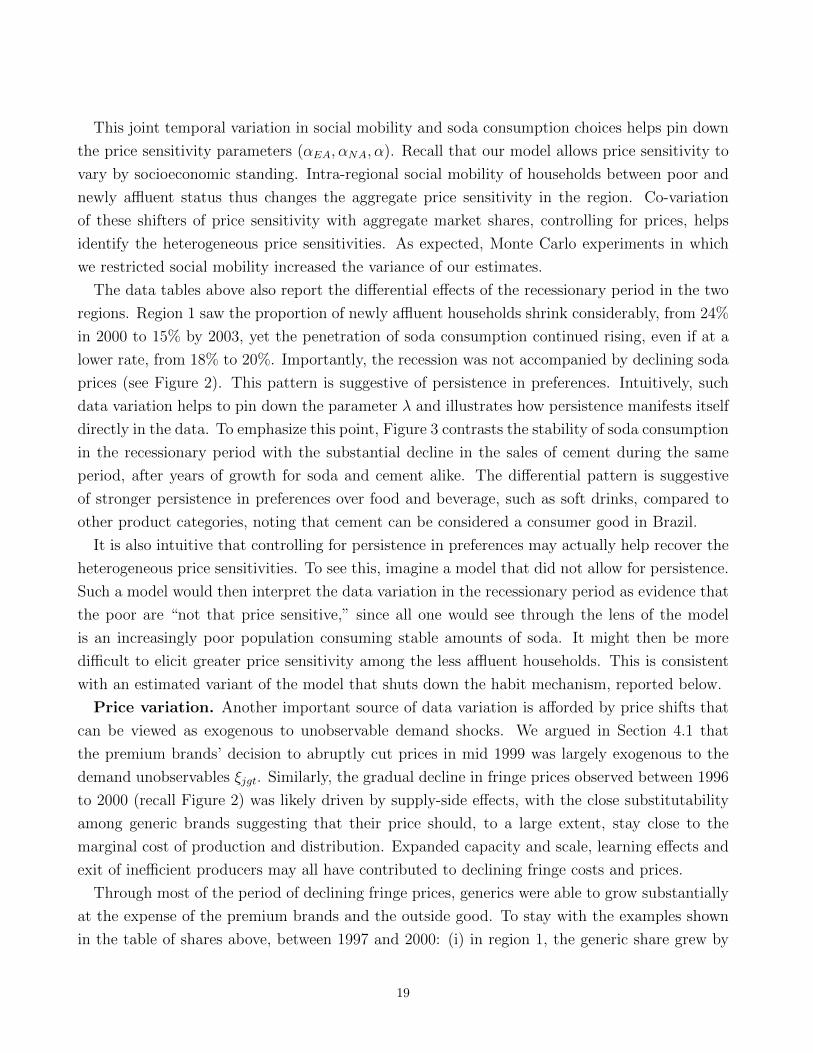
This joint temporal variation in social mobility and soda consumption choices helps pin down
the price sensitivity parameters (αEA, αNA, α). Recall that our model allows price sensitivity to
vary by socioeconomic standing. Intra-regional social mobility of households between poor and
newly affluent status thus changes the aggregate price sensitivity in the region. Co-variation
of these shifters of price sensitivity with aggregate market shares, controlling for prices, helps
identify the heterogeneous price sensitivities. As expected, Monte Carlo experiments in which
we restricted social mobility increased the variance of our estimates.
The data tables above also report the differential effects of the recessionary period in the two
regions. Region 1 saw the proportion of newly affluent households shrink considerably, from 24%
in 2000 to 15% by 2003, yet the penetration of soda consumption continued rising, even if at a
lower rate, from 18% to 20%. Importantly, the recession was not accompanied by declining soda
prices (see Figure 2). This pattern is suggestive of persistence in preferences. Intuitively, such
data variation helps to pin down the parameter λ and illustrates how persistence manifests itself
directly in the data. To emphasize this point, Figure 3 contrasts the stability of soda consumption
in the recessionary period with the substantial decline in the sales of cement during the same
period, after years of growth for soda and cement alike. The differential pattern is suggestive
of stronger persistence in preferences over food and beverage, such as soft drinks, compared to
other product categories, noting that cement can be considered a consumer good in Brazil.
It is also intuitive that controlling for persistence in preferences may actually help recover the
heterogeneous price sensitivities. To see this, imagine a model that did not allow for persistence.
Such a model would then interpret the data variation in the recessionary period as evidence that
the poor are “not that price sensitive,” since all one would see through the lens of the model
is an increasingly poor population consuming stable amounts of soda. It might then be more
difficult to elicit greater price sensitivity among the less affluent households. This is consistent
with an estimated variant of the model that shuts down the habit mechanism, reported below.
Price variation. Another important source of data variation is afforded by price shifts that
can be viewed as exogenous to unobservable demand shocks. We argued in Section 4.1 that
the premium brands’ decision to abruptly cut prices in mid 1999 was largely exogenous to the
demand unobservables ξjgt. Similarly, the gradual decline in fringe prices observed between 1996
to 2000 (recall Figure 2) was likely driven by supply-side effects, with the close substitutability
among generic brands suggesting that their price should, to a large extent, stay close to the
marginal cost of production and distribution. Expanded capacity and scale, learning effects and
exit of inefficient producers may all have contributed to declining fringe costs and prices.
Through most of the period of declining fringe prices, generics were able to grow substantially
at the expense of the premium brands and the outside good. To stay with the examples shown
in the table of shares above, between 1997 and 2000: (i) in region 1, the generic share grew by
19

5 points, with the premium share (i.e., 1− sgen − s0) holding up quite well; and (ii) in region 4,
the generic share grew by 6 points, and at the expense of the premium share. Intuitively, the
co-movement in prices and shares is picked up by the parameters that govern price sensitivity
and habit formation, thus contributing to their identification.
The table also suggests that the generic share in regions 1 and 4 held up quite well following
the premium price cut in mid 1999 (see Figure 2 for all regions combined). This provides
further evidence of persistence in preferences and, specifically, it helps identify our Brand Type
Persistence (BTP) mechanism: a habit of “going generic,” developed by part of the population
prior to the mid-1999 premium price cut, made it very difficult for premium brands to win such
households over, even via a drastic price cut. The price cut did, however, help protect premium
brands from further market share losses, in part by attracting households who, at the time, had
a “no soda” habit. We return to this discussion in the results section. To sum, wide variation
in the socioeconomic composition of households and the sharp price cut help us identify both
heterogeneous price sensitivities and our habit mechanism.
5 Results
5.1 Estimates from the demand model
Table 3 reports estimates for our demand model. The price sensitivity of poor households has
the expected negative sign and is precisely estimated at -5.7. The parameters αEA and αNA are
positively signed, with αEA > αNA. Recalling that (α + αEA) and (α + αNA) capture the price
sensitivities of the two affluent groups, this implies that the established affluent are the least
price sensitive group, the poor are the most sensitive group, and the newly affluents display an
intermediate level of sensitivity. Namely, α + αEA = −2.1 (with a standard error of 0.2) for the
established affluent, and α + αNA = −3.9 (with a standard error of 0.6) for the newly affluent.
This ranking is consistent with the Financial Times article referenced in the introduction.
In terms of statistical significance, the newly affluent are marginally less price sensitive than
the poor (the p-value of a test of equality is 0.10) but significantly more price sensitive than the
established affluent (the p-value of a test of equality is 0.00).25 We discuss the economic signifi-
cance of these estimated parameters below when we examine demand elasticities and conduct a
counterfactual experiment.26
We find strong evidence for the second mechanism we study in this paper—habit formation.
The coefficient λ is estimated to be positive and it is very precisely estimated. As we note
25This follows from the estimates reported in Table 3, namely αNA = 1.8, s.e. 1.4 and αEA − αNA = 1.8, s.e. 0.5.26The appendix reports robustness checks. Across the bulk of specifications we tried, the exact point estimate for αNA is less
robust when compared to other parameter estimates, but the finding that it does not exceed αEA (i.e., newly affluents are no lessprice sensitive than established affluents) holds rather consistently.
20

in the appendix, this finding is robust across different specifications.27 In terms of economic
significance, our utility framework provides a measure of the increased willingness to pay for
generic (premium) soda that results from previous consumption of generic (premium) soda. In
particular, the implied increase for a newly affluent household is −λ/ (α + αNA) = 1.1 R$/liter.28
Further, the implied increase in willingness to pay for a generic over a premium brand when the
household has a generic habit rather than a premium habit is twice this amount.
Such measures suggest a substantial monetary value for habit formation, and a crucial role
played by this mechanism in emerging market dynamics. Once a newly affluent (or other)
household develops a generic habit, “convincing” it to switch to a premium product becomes
substantially more difficult. In the wake of an emerging middle class and declining fringe prices,
our estimated model helps explain the sense of urgency with which premium brands acted in
mid 1999, as we argue in the counterfactual analysis below.
Table 3 further reports the effects of several shifters of δjgt, the base utility of consuming brand
j in region-period market gt. Our specification includes the effects of brands’ media advertising
and in-store presence.29 In either case, we interact the brand-region-period varying “visibility”
variable with regional dummy variables, allowing effects to differ across regions. For instance,
in the case of advertising, this might reflect cross-sectional variation in households’ exposure to
media, and the fact that these measures pertain only to the main cities within each region (so they
are not comparable across regions). We generally obtain positive effects for media advertising
and for in-store presence.
Coefficients on (similarly region-specific) time trends tend to be negative. Such negative effects
are consistent with continued improvement in the value of the outside option, which includes
beverages other than soda such as juices and (tap or bottled) water, concomitant with the
overall trend of economic growth.30 Finally, note that our specification controls for 9 × 7 = 63
brand-region fixed effects, capturing the tendencies of particular regions to consume different
brands (e.g., historically, tastes for Pepsi are known to be relatively strong in the South, region
6—see Table 1). We also control for bi-monthly seasonality effects interacted with brand type,
to allow these effects to differ across premium and generic brands. Over and above seasonality,
27One possible interpretation for persistence in market shares could be serial correlation in the demand shocks ξ. Our inclusion ofbrand-region fixed effects and region-specific trends alleviates this concern. Just the same, calculating the simple correlation betweencurrent-period and previous-period estimated values for ξ for each brand-region combination yields correlations that are mostlynegative (52 out of 63) and mostly small in absolute value. Of the six correlations that exceed 0.2 (with a maximum correlation of0.5), five are in region 1, and they do not pertain to the leading brands Coke, Guarana Antarctica and Fanta.
28Corresponding amounts for established affluent and poor households are 2.0 and 0.7 R$/liter, respectively.29The appendix further discusses these covariates and reports robustness tests in which they are dropped from the specification.
To gain a sense of variation in premium brands’ advertising, intensity for the Coke brand in Sao Paulo Metro was measured at 2199Gross Rating Points in December 2000, rising to 3587 GRP in December 2001, whereas Pepsi’s GRP were 351 and 598 in theserespective periods. Media advertising in the fringe is measured at zero GRP throughout.
30Forbes (2004) reports that the “the juice category grew twenty times over the past decade, albeit from a low base.” IBGE’sannual household surveys (PNAD) also indicate a sustained increase in access to tap water and piped sewerage in urban Brazil. Notethat we rescale variables to vary between 0 and 1, so the trend coefficients reflect variation from the start to the end of the sample:these effects are economically small.
21

market gt’s mean temperature is estimated to have a significantly positive effect on demand.31
To further explore the economic implications of our demand estimates, Table 4 reports esti-
mated own-price elasticities. The table lists both aggregate elasticities for the leading brands,
and elasticities by household type for Coke and for generics, reporting means over all region-
period markets gt.32 A 1% increase in Coke’s price lowers its market share by 1.7%, compared
with somewhat larger (in magnitude) elasticities of −2.0 to −2.1 for the other premium brands,
Guarana Antarctica, Fanta and Pepsi. The own-price elasticity for generics is −0.7. While this
value may seem low, note that this is the elasticity of demand for the aggregation of generic
brands. The demand for each individual generic brand should be much more elastic, given the
limited differentiation and fierce price competition within the fringe.
Examining the nine type-specific elasticities, and fixing the habit state, we see that demand
becomes more elastic the lower is the socioeconomic standing. For instance, considering house-
holds with a premium habit, Coke elasticities are (-1.4,-3.3,-5.7) for the established affluent,
newly affluent, and poor groups, respectively. Fixing the socioeconomic standing, the habit state
has a strong impact on demand elasticities. Considering, for example, the newly affluent group,
demand for Coke is least elastic for households with a premium habit -3.3. Households with
either generic or “no-soda” habits exhibit higher elasticities of roughly -4.2.
The evolution of these type-specific own-price elasticities is shown in Figure 5 (for region 4).
The left panel considers the Coke brand. Demand by all types becomes less elastic halfway
through the sample, when premium brands cut prices. The least elastic demand for Coke is
by the established affluent with a premium habit; the most elastic demand is by the three poor
types, particularly those who did not consume premium soda previously. Coke elasticities among
newly affluent types lie between the elasticities displayed by the established affluent and the
poor. The picture underscores the important role we infer for habit formation: members of the
emerging middle class who have developed a premium habit display price sensitivities for Coke
that are “half way” between newly affluents who have not developed such a habit and the more
sensitive among the rich. The right panel depicts own-price elasticities for generics. The demand
for generics is less elastic among newly affluent types who have already “gone generic” than
among established affluent types who have not yet been “grabbed,” once again demonstrating
the important role played by persistent preferences.
Table 5 continues to describe the economic implications of our estimated demand model.
31To illustrate within-season variation in temperature, winter temperatures in the South region averaged 15.1oC in July 2001against 12.1oC in July 2000.
32The household type-r specific own-price (j = k) and cross-price (j 6= k) elasticities of demand for brand j are computed fromηjk,r,gt =
(∂sj,r,gt/∂pkgt
) (pkgt/sj,r,gt
)where, for brevity, we omit the argument θ, and,
∂sj,r,gt
∂pkgt=
(α+ αr) sj,r,gt (1− sj,r,gt) if j = k− (α+ αr) sj,r,gtsk,r,gt if j 6= k
22

Panel A reports predictions for the share of households purchasing soda, by type of household
and brand. Overall soda penetration is 69%, 22% and 5% for the established affluent, the newly
affluent and the poor, respectively (these are means computed across all regions over the last
12 months of the sample). Compared to the established affluent, newly affluent households are
more likely to favor generic over premium brands: generic-to-premium consumption ratios are
0.5, 1.4 and 2.7 for the established affluent, newly affluent and poor groups, respectively. Panel
B provides transition matrices that further underscore the persistence in preferences: a newly
affluent household who established a premium (generic) habit in the previous period consumes
premium (generic) soda in the current period with a probability of 0.66 (0.73). For the established
affluent, these probabilities are even higher (0.90 and 0.87, respectively).
A “no habit” model variant. Table 6 presents results from a variant of our demand model
which shuts down the habit formation mechanism by constraining λ to equal zero. Estimates
from this model imply that the newly affluent are more price sensitive than the poor. This
stands in contrast to the findings of our baseline model, whose predictions we view as more
realistic. The demand surge observed beginning in 1996 across many consumer goods markets,
soft drinks being one of them, suggests that Brazil’s emerging middle class was less, not more,
price sensitive than the poor. The estimated no-habit model suggests that the emergence of
a new middle class changed the aggregate price sensitivity in the “wrong” direction, missing
the phenomenon which is at the heart of our study: an expansion in demand stemming from a
socioeconomic transformation.
The downward bias in the poor’s price sensitivity in the model variant is consistent with the
intuition provided in Section 4.2 above: during the recession in the later part of the sample,
households moved down from newly affluent to poor status, yet soda consumption remained
stable. By not allowing a habit mechanism, the restricted model appears to interpret this as
evidence that the poor are not very price sensitive. This further demonstrates the importance
of accounting for persistence in preferences.
5.2 Counterfactual analysis of the premium price cut
A striking feature of the data is the premium brands’ sharp price cut, led by Coca-Cola, almost
halfway through the sample period. As the solid lines in the left panel of Figure 6 indicate (for
region 5, with similar variation for other regions), per-liter premium brand prices stayed broadly
flat at about R$ 1.15 until mid 1999, then dropped abruptly to R$ 0.90 and stayed at this lower
level. Fringe prices, in contrast, experienced a prolonged, gradual decline from R$ 0.80 to R$
0.55 between late 1996 and mid 2000. The picture reveals that fringe prices did not deviate from
their downward trend in response to the premium price cut, consistent with fringe prices closely
tracking their producers’ marginal costs.
23

We employ the estimated model to simulate the evolution of market shares had premium
sellers not cut prices in mid 1999. This counterfactual price path is marked by the dashed line
in the left panel of Figure 6. In this analysis, we keep fringe prices equal to the ones observed in
the data. This assumption is justified by the fringe’s competitive nature and, as discussed, the
absence of an apparent pricing response to the premium price cut.
The right panel of Figure 6 reports the estimated impact on aggregate premium and generic
market shares. Observed shares are marked by solid lines, whereas counterfactual shares are
marked by dashed lines (shares in this figure are out of the total market size, which includes
the outside option, so that the premium and generic shares do not sum to one). A clear picture
emerges: had premium producers failed to cut prices, they would have suffered a deep loss of
market share, hitting a rock bottom in the winter of 2000. At that point, the premium share
would have been 12%, compared to a share of over 20% in the observed sample.
In the counterfactual scenario, generic brands grow relentlessly at the expense of their premium
competitors. The figure reports that the generic market share would have surpassed the premium
share early in 2000. By 2003, generics in region 5 would have enjoyed a market share advantage
over premium brands of 9% (25% against 16%).
This analysis provides support for Coca-Cola’s price cut, in that it seems to have prevented
a substantial drop in market share. A key insight from the analysis is that the premium price
cut was especially effective in terms of attracting customers who otherwise would have chosen
the outside, “no soda” option. It was only partially effective in converting consumers of generic
brands into premium consumption. This can be inferred by comparing the actual versus counter-
factual shift in the premium shares over time to the smaller corresponding shift in generic shares.
For example, actual inside shares over 2001-02 averaged 46% (28% premium plus 18% generic) to
be compared with counterfactual inside shares of 40% (17% premium plus 23% generic). This is
suggestive of substantial market segmentation, consistent with state dependence that limits the
scope for “business stealing” across the types of brand offerings and the high monetary value of
habit formation. Still, in the absence of premium brands cutting prices, the fringe’s penetration
would have been almost 30% larger (i.e., (23− 18)/18).
Impact on variable profit. While our analysis indicates that Coca-Cola’s price cut suc-
ceeded in avoiding a deep market share loss, we note that this was achieved at a cost: a deep
price cut of over 20%. In other words, premium sellers sacrificed a non-negligible portion of their
margins to protect their market shares.33 To assess the impact of the price cut on earnings, we
perform a back-of-the-envelope calculation of variable profit both in the observed sample, and
under the counterfactual no-price-cut scenario.
Using information gleaned from Ambev’s local SEC filings, and from conversations with in-
33Protecting market shares, even at a high cost, may be rational insofar as current market share is an “asset,” predictive of futureprofit. See Bronnenberg, Dhar and Dube (2009) on the persistence of brand market shares.
24

dustry insiders, among other sources, we estimate that the premium brands’ combined variable
profits (excluding fixed costs) during the first three years after the price drop amounted to R$
861 million, to be compared to counterfactual profits of R$ 807 million, had the price cut not
occurred.34 That is, a 6% loss in variable profit, considering only the medium run, was avoided
by the premium price cut. The evidence supports the notion that the price cut was beneficial in
terms of its impact on both market shares and profits.
A comparison with the “no habit” model variant. To further explore the role played
by the habit mechanism, we perform the same counterfactual analysis but using estimates from
the no-habit model variant presented above. The results are displayed in Figure 7. Comparing
Figure 7 to Figure 6, we learn that, relative to the baseline model, the no-habit model predicts a
substantially smaller erosion of market share for premium brands had they failed to cut prices.
Further, using the same back-of-the-envelope calculations discussed above, the no-habit model
implies that the price cut actually decreased premium brands’ variable profit, from R$ 1,013
million (with no price cut) to R$ 861 million (with price cut) over the same three years. This
stands in stark contrast to the predictions of the baseline model.
Discussion. The counterfactual analysis lends strong justification to Coca-Cola’s strategic
price cut. Importantly, this conclusion is delivered by the baseline model but not by the no-habit
variant, a finding that we interpret to be indicative of the role played by state dependence in
this emerging market. Our estimates suggest that habit carries a large monetary value. Once
a newly affluent household “goes generic,” it is significantly less likely to switch into premium
soda consumption, and vice versa. The arrival into the market of millions of new customers, who
have yet to form persistent consumption patterns, provides an opportunity for generic producers
to challenge the position of established brands.
Our analysis suggests that the main effect of the premium sellers’ price cut was not to convert
households with the generic habit into consumption of their products. Rather, the price cut’s
main effect was to tap into the large pool of households with the no-soda habit. By inducing a
substantial portion of these households to develop a habit of consuming premium soda, Coca-
Cola and Ambev were able to shield themselves against further losses. The analysis suggests
that it is this mechanism that stabilized market shares after mid 1999, despite the decline in
fringe prices continuing for another year (recall Figure 2). The ability to draw such conclusions
stems from implementing a rich utility framework that allows for both heterogeneity in price
sensitivity and for persistent preferences. A standard no-habit variant appears ill-suited to a
rapidly changing market as ours.
34See the appendix for details on how this calculation was performed.
25

6 Concluding remarks
This paper examines two salient features of the Brazilian soft-drink market: the emergence of a
new middle class, and the rapid growth of a generic fringe. Using mainly aggregate data that
exhibit very rich variation, we estimate a household choice model that highlights two aspects
which we view as highly important in such markets: the heterogeneous price sensitivities of
different socioeconomic groups, and habit formation in household preferences.
The Brand Type Persistence mechanism that we specify captures a world in which premium
brands are prompted to cut prices in the wake of an emerging middle class. If they fail to do
this, a substantial mass of the “new customers” might be captivated by the generic habit. It
may then prove much more difficult to convince these consumers to pay substantially more for a
highly advertised premium brand.
While our application focuses on the Brazilian soft-drink market, we view the issues tackled in
this work as highly pertinent to many consumer goods markets in the developing world, where
a tension between advertised branded offerings and discounted generics exists or is developing.
Understanding the features of demand and the nature of competition in such markets should be
of great interest for policymakers and firms alike.
References
[1] ABEP, Brazilian Association of Market Research Firms (2003). Criterio de classificacao
economica Brasil: Sistema de pontos. ABEP Publication, Sao Paulo. (Points system for
classifying households into economic segments: Brazil criteria, in Portuguese.)
[2] Ambev (2003). Informacoes anuais (IAN). Comissao de Valores Mobiliarios, CVM. (Annual
report to Brazil’s Securities and Exchange Commission, in Portuguese.)
[3] Anderson, E. T., K. T. Hansen and K. Misra (2012). Estimating heterogeneity and state
dependence with aggregate data. Mimeo, Northwestern University and London Business
School
[4] Atkin, D. (2011). Trade, tastes and nutrition in India. American Economic Review, forth-
coming
[5] Bils, M. and P. J. Klenow (2004). Some evidence on the importance of sticky prices. Journal
of Political Economy 112, 947-985
[6] Boston Consulting Group (2002). Mercados pouco explorados: Descobrindo a classe C.
BCG Publication, Sao Paulo. (Under-explored markets: Discovering the “C” class, in Por-
tuguese.)
26

[7] Berry, S., J. Levinsohn, and A. Pakes (1995). Automobile prices in market equilibrium.
Econometrica 63, 841-90
[8] Berry, S., M. Carnall, and P. T. Spiller (1996). Airline hubs: Costs, markups and the
implications of consumer heterogeneity. NBER working paper 5561
[9] Bresnahan, T. F. (1997a). Valuation of new goods under perfect and imperfect competition:
A comment, in Bresnahan, T. F. and R. Gordon (eds.), The Economics of New Goods,
Studies in Income and Wealth Vol. 58. National Bureau of Economic Research, Chicago
[10] Bresnahan, T. F. (1997b). The Apple Cinamon Cheerios war: Valuing new goods, identifying
market power, and economic measurement. Mimeo, Stanford University
[11] Bronnenberg. B., S. Dhar and J.-P. Dube (2009). Brand history, geography, and the persis-
tence of brand shares. Journal of Political Economy 117, 87-115
[12] Bronnenberg. B., J.-P. Dube and M. Gentzkow (2012). The evolution of brand preferences:
Evidence from consumer migration. American Economic Review 102, 2472-2508
[13] Calzolari, G., A. Ichino, F. Manaresi, and V. Nellas (2012). When the baby cries at night:
Uninformed and hurried buyers in non-competitive markets. CEPR working paper DP8856
[14] Carvalho Filho, I. and M. Chamon (2012). The myth of post-reform income stagnation:
Evidence from Brazil and Mexico. Journal of Development Economics 97, 368-386
[15] Chaudhuri, S., P. K. Goldberg and P. Jia (2006). Estimating the effects of global patent
protection in pharmaceuticals: A case study of quinolones in India. American Economic
Review 96, 1477-1514
[16] Dube, J.-P., G. J. Hitsch, P. E. Rossi and M. A. Vitorino (2008). Category pricing with
state-dependent utility. Marketing Science 27, 417-429
[17] Economist (2007). Adios to poverty, hola to consumption: Faster growth, low inflation,
expanding credit and liberal trade are helping to create a new middle class in Latin America.
Print edition of August 18, 2007
[18] Economist (2011a). Politics in emerging markets: The new middle classes rise up. Print
edition of September 3, 2011
[19] Economist (2011b). Indonesia’s middle class: Missing BRIC in the wall. Print edition of
July 21, 2011
[20] Economist (2012). China’s motor industry: Stepping on the gas. Edition of April 24, 2012
[21] Eichenbaum, M. S., L. P. Hansen and K. J. Singleton (1988). A time series analysis of repre-
sentative agent models of consumption and leisure choice under uncertainty. The Quarterly
Journal of Economics 103, 51-78
[22] Erdem, T. (1996). A dynamic analysis of market structure based on panel data. Marketing
Science 15, 359-78
[23] Horsky, D., P. Pavlidis and M. Song (2012). Incorporating state dependence in aggregate
27

brand-level demand models. Mimeo, University of Rochester
[24] Ferreira, F. H. G., J. Messina, J. Rigolini, L.-F. Lopez-Calva, M. A. Lugo and R. Vakis
(2012). Economic Mobility and the Rise of the Latin American Middle Class. World Bank,
Washington D.C.
[25] Financial Times (1999). Brazil’s regional drinks makers slake thirst for value: The tax regime
and growing demand have penalised leading brands. Edition of June 16, 1999
[26] Forbes (2004). Segmento de sucos cresceu 20 vezes nos ultimos dez anos, mas brasileiro ainda
consome pouco. (Juice category grew twenty times over the past decade, yet Brazilians still
consume little, in Portuguese.) Edition of February, 2004
[27] Frankel, D. M. and E. D. Gould (2001). The retail price of inequality. Journal of Urban
Economics 49, 219-239
[28] Galanz (2008). Galanz household electric appliances: the unruly competition in the market
will hopefully end. ‘Corporate News’ posted on the company’s website, dated September 1,
2008
[29] Hausman, J. A., G. K. Leonard and J. D. Zona (1994). Competitive analysis with differen-
tiated products. Annales D’Economie et de Statistique 34, 159-80
[30] Hurwitz, M. A. and R. E. Caves (1988). Persuasion or information? Promotion and the
shares of brand name and generic pharmaceuticals. Journal of Law and Economics 31, 299-
320
[31] Kalouptsidi, M. (2010). From market shares to consumer types: Duality in differentiated
product demand estimation. Journal of Applied Econometrics 27, 333-342
[32] Keane, M. P. (1997). Modeling heterogeneity and state dependence in consumer choice
behavior. Journal of Business & Economic Statistics 15, 310-27
[33] Lach, S. (2007). Immigration and prices. Journal of Political Economy 115, 548-587
[34] Nair, H. (2007). Intertemporal price discrimination with forward-looking consumers: Appli-
cation to the US market for console video-games. Quantitative Marketing and Economics 5,
239-92
[35] Neri, M. (1995). Sobre a mensuracao dos salarios reais em alta inflacao. (About the measure-
ment of real wages under high inflation, in Portuguese.) Pesquisa e Planejamento Economico
25, 497-525
[36] Nevo, A. (2000). A practitioner’s guide to estimation of random coefficients logit models of
demand. Journal of Economics & Management Strategy 9, 513-548
[37] Nevo, A. and Konstantinos Hatzitaskos (2006). Why does the average price paid fall dur-
ing high demand periods? Mimeo, Northwestern University and University of California,
Berkeley
[38] Salvo, A. (2009). Cut-throat fringe competition in an emerging country market: Tax evasion
28
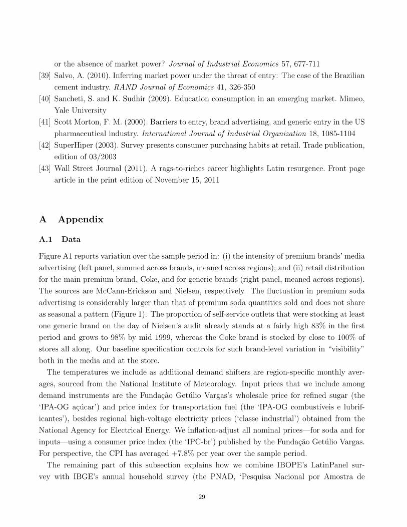
or the absence of market power? Journal of Industrial Economics 57, 677-711
[39] Salvo, A. (2010). Inferring market power under the threat of entry: The case of the Brazilian
cement industry. RAND Journal of Economics 41, 326-350
[40] Sancheti, S. and K. Sudhir (2009). Education consumption in an emerging market. Mimeo,
Yale University
[41] Scott Morton, F. M. (2000). Barriers to entry, brand advertising, and generic entry in the US
pharmaceutical industry. International Journal of Industrial Organization 18, 1085-1104
[42] SuperHiper (2003). Survey presents consumer purchasing habits at retail. Trade publication,
edition of 03/2003
[43] Wall Street Journal (2011). A rags-to-riches career highlights Latin resurgence. Front page
article in the print edition of November 15, 2011
A Appendix
A.1 Data
Figure A1 reports variation over the sample period in: (i) the intensity of premium brands’ media
advertising (left panel, summed across brands, meaned across regions); and (ii) retail distribution
for the main premium brand, Coke, and for generic brands (right panel, meaned across regions).
The sources are McCann-Erickson and Nielsen, respectively. The fluctuation in premium soda
advertising is considerably larger than that of premium soda quantities sold and does not share
as seasonal a pattern (Figure 1). The proportion of self-service outlets that were stocking at least
one generic brand on the day of Nielsen’s audit already stands at a fairly high 83% in the first
period and grows to 98% by mid 1999, whereas the Coke brand is stocked by close to 100% of
stores all along. Our baseline specification controls for such brand-level variation in “visibility”
both in the media and at the store.
The temperatures we include as additional demand shifters are region-specific monthly aver-
ages, sourced from the National Institute of Meteorology. Input prices that we include among
demand instruments are the Fundacao Getulio Vargas’s wholesale price for refined sugar (the
‘IPA-OG acucar’) and price index for transportation fuel (the ‘IPA-OG combustıveis e lubrif-
icantes’), besides regional high-voltage electricity prices (‘classe industrial’) obtained from the
National Agency for Electrical Energy. We inflation-adjust all nominal prices—for soda and for
inputs—using a consumer price index (the ‘IPC-br’) published by the Fundacao Getulio Vargas.
For perspective, the CPI has averaged +7.8% per year over the sample period.
The remaining part of this subsection explains how we combine IBOPE’s LatinPanel sur-
vey with IBGE’s annual household survey (the PNAD, ‘Pesquisa Nacional por Amostra de
29

Domicılios’) to produce household counts by socioeconomic standing. We also detail how we
obtain the first period’s type-distribution vector, Fg1, from IBGE’s 1995/96 urban household
expenditure survey (the ‘Pesquisa de Orcamentos Familiares’).
Data on aggregate social mobility. From IBOPE’s LatinPanel we observe, for every region-
year pair, what proportion of urban households belong to each of two socioeconomic groups,
ABC or DE. IBOPE’s regions map directly into Nielsen’s seven regions, with the exception of
region 1 (northeastern states less Maranhao and Piauı) for which IBOPE’s coverage includes all
northeastern and northern states. Since Maranhao, Piauı and the North comprise the country’s
least urbanized and least populated area, we simply take IBOPE’s urban distributions for the
Northeast/North as representative of urban households in Nielsen’s region 1. IBOPE’s survey
through 2002 was representative of all municipalities with populations of at least 20,000, and their
coverage was expanded in 2003 to represent municipalities with populations exceeding 10,000.
We obtain household counts from IBGE’s annual household surveys (PNAD). These cover
households, both urban and rural, in all 27 states of the country. For perspective, 115,654
households were sampled in 1999. We use the weights provided to expand the representative
sample to the universe of households. We consider only households residing in urban areas and
in states within each Nielsen region. For example, for region 1, we sum the number of urban
households across all states in the Northeast less Maranhao and Piauı.
We then multiply, for each Nielsen region and year, the IBOPE socioeconomic proportions of
urban households by the IBGE urban household counts. To increase the frequency of the resulting
panel from annual to monthly periods (or bimonthly periods, thus matching the frequency of
Nielsen’s point-of-sale audits), we linearly interpolate from September of one year to September
of the following year, noting that September is the IBGE PNAD’s annual “month of reference.”
Data on household-level brand choices. IBGE’s HEX 95/96 surveyed 16,013 households
in 11 large metropolitan areas across the country. Carvalho Filho and Chamon (2012) discuss this
survey in detail. Over a reference period of one week falling between October 1995 and Septem-
ber 2006, the soft drink expenditure in R$ for consumption inside the home was recorded for each
household, detailed by soda brand(s) purchased. We then classified the following brand descrip-
tions and codes as “premium” brands: Coca-Cola (9301); Pepsi (9302); Guarana (9303); Fanta
laranja, uva, limao (9304); Soda limonada (9307); Mirinda (9308); Sukita (9315); Pop laranja
(9316); and Refrigerante agua tonica (9349). Examples of coded brand descriptions that we clas-
sified as “generic” brands are: Refrigerante tubaına (9318); Refrigerante laranja exceto Fanta,
Sukita, Pop, Crush (9339); Refrigerante cola exceto Coca-Cola e Pepsi-Cola (9340); Refriger-
ante caju qualquer marca (9346); and Refrigerante Goianinha (9355). Of the 16,013 households,
10,172 (or 64% of households) were recorded as making no soda purchases, 4,465 households
(28%) purchased only brands that we can confidently identify as premium, 310 households (2%)
30

purchased only brands that we identify as generic, and 236 households (only 1%) simultaneously
purchased brands that we identify as premium and brands that we identify as generic. This
observation justifies our modeling of soda-consuming households at each point in time as either
premium or generic shoppers, but not “hybrids.”
We deemed four soda descriptions to be ambiguous with regard to brand type: Refrigerante
agua natural (9310); Refrigerante gasosa (9319); Refrigerantes nao especificado (9335); and
Refrigerante dietetico (9360). We need to assign the soda expenditure of the remaining 830
soda-purchasing households (5% of the survey sample) to either premium brands or generic
brands. These are households whose soda expenditure we cannot entirely identify by brand
type, such as a household purchasing R$ 4 of Coke (9301) and R$ 2 “Soda not specified” (9335).
To do this, we first designate as premium the “brand-unidentifiable” soda expenditure portion
(R$ 2 in the example) for those households whose identifiable-premium expenditure share of
soda exceeds 50% (Coke’s 67% share in the example) and identifiable-generic expenditure share
of soda is less than 10% (0% in the example). Similarly, we assign to generic the unidentifiable
soda expenditure portion for those identified-generic-dominant households. Finally, the soda
expenditure portion that for a remaining 614 households is still not assigned to a brand type—
e.g., a yet-to-be-assigned R$ 4 purchase of “Soda not specified” (9335)—is allocated among
premium and generic expenditure: (i) in proportion to the (identified or designated) premium
versus generic expenditure shares within the household; or (ii) if none of the household’s soda
expenditure is identifiable (say the household in this second example purchased only “Soda not
specified”), the allocation is done in proportion to the premium versus generic expenditure shares
across households in the same socioeconomic group and metropolitan area.
We use balance sheet data to classify households according to socioeconomic standing, ABC or
DE, as described in Section 2. We use the weights provided to expand the representative sample
to a universe of 12.5 million households across the 11 metropolitan areas. To calculate household-
level premium and generic quantities, we divide HEX 95/96 expenditures on premium and generic
soda by Nielsen’s region-specific share-weighted mean prices for premium and generic brands,
respectively, in period t = 1 (Dec-96/Jan-97). We then aggregate premium (resp., generic)
quantities across the universe of households in each socioeconomic segment and in the surveyed
metropolitan areas for each Nielsen region g (e.g., the cities of Recife, Fortaleza and Salvador in
the Northeast, g = 1).
The premium (resp., generic) soda shares among the initial masses of established affluent and
poor households are calculated analogously to how we define sjgt = qjgt/Mgt in Section 2, i.e.,
taking market size (in our base specification) as six liters per household per week times the number
of weeks in period t = 1. Combining these premium versus generic (versus no soda) shares by
socioeconomic group with first-period household counts by socioeconomic group (as per above),
31

yields FEAA,g1, FPA,g1 and FEAB,g1, FPB,g1 (recall that FNAA,g1 = FNAB,g1 = 0). We consider only
soda purchases that were recorded as being for the household’s inside-the-home consumption
(rather than recorded as “individual consumption”) and at stores coded as Supermercado (1),
Hipermercado (2), Padaria (3), Lanchonete (11), and Mercado & Central de Abastecimento (26),
in view of the mapping to Nielsen’s self-service channel (stores with checkouts).
Two points are noteworthy. First, the HEX survey suggests that urban household size does
not vary significantly across socioeconomic group. Mean household sizes are 3.64 for ABC (with
a standard deviation of 1.58) and 3.76 for DE (s.d. 1.99). Second, while the HEX shares that
enter the initial conditions Fg1 are calculated following the market share definition of Section 2,
one should note that the shares reported in Table 2 are extensive margins of soda consumption,
i.e., the proportions of households who purchase any soda quantity. As for intensive margins,
the modal intensity of soda consumption, conditional on positive consumption, is 2 liters per
household per week regardless of the socioeconomic group and the region. One can intuitively
interpret this pervasive intensive margin as “one 2-liter family-size bottle of soda that is brought
to the table every week.”
We performed all manner of “consistency checks,” where applicable, to ensure that the data
were consistent across the different sources. For example, among households residing in the
three metropolitan areas in the Northeast that were surveyed in the HEX, premium and generic
market shares amount to 12.5% and 0.4%, respectively.35 These HEX shares of 12.5% and 0.4%
are similar to the Nielsen market shares of 12.3% across premium brands and 0.3% for generics
in the Dec-96/Jan-97 bimonth (soda sold in family-size bottles through self-service outlets in the
Northeast). By way of another example, the HEX 95/96 projects the universe of households for
region 3 (the Rio de Janeiro metropolitan area) at 2.96 million (Table 2), to be compared to
2.64 million households projected for Dec-96 in the IBGE PNAD (noting that Nielsen’s region
3, which we adopt for the IBGE household counts, excludes some peripheral villages around the
city of Rio de Janeiro). Further, using the HEX 95/96’s balance sheet data, we assigned ABC
socioeconomic status to 55% of region 3’s households (Table 2), whereas the IBOPE data suggest
that at that time 57% of region 3’s households were ABC.
A.2 Further estimation details
A.2.1 Dynamic type evolution
We provide examples, from the data, of the dynamic updating process. We consider two tran-
sitions, both for region 4 (the Sao Paulo metropolitan area). The first transition, from t = 1
to t = 2, features upward mobility and, unusually in the data (yet we need to allow for this),
35These shares are as defined in Section 2. Shares grow to 26.6% and 0.7%, respectively, if we condition on ABC households (theseare similar to the extensive margins reported in Table 2).
32

a slight flow of residents out of the region (“net urban-to-rural migration”). The second transi-
tion, from t = 10 to t = 11, features upward mobility and the rural-to-urban migration that is
prevalent in the data. We illustrate these transitions at the estimated model parameters θ∗. We
also comment on the robustness of our estimates to the baseline mobility Assumptions 1 and 2.
Region 4, t = 1 to t = 2. The initial type-distribution vector is
Fg=4,t=1 =FEAA,4,1, FEAB,4,1, FEAO,4,1, FNAA,4,1, FNAB,4,1, FNAO,4,1, FPA,4,1, FPB,4,1, FPO,4,1
= 0.255, 0.029, 0.361, 0, 0, 0, 0.048, 0.009, 0.299
As explained, the last element, for instance, is the product of (region 4’s) poor household count in
t = 1 (observed from combining IBOPE and IBGE) and the share of the outside option among
region 4’s DE households (calculated from the HEX 95/96), divided by the total household
count (IBOPE/IBGE), i.e., 1346585×0.84093/3789771 ' 0.299. From sj,r,g=4,t=1(θ∗) (see (4)), we
obtain the mass of households for each of the nine types who choose to consume premium, generic,
or no soda. For example, the share of premium soda among established affluent households who
have a premium habit,∑
j∈A sj,EAA,g=4,t=1(θ∗) ' 94%. In contrast, the shares of premium soda
among established affluents with generic habits and no-soda habit are 3% and 20%, respectively.
Thus, since the established affluent population is constant over time (at 2443186), the number
of established affluent households going into t = 2 with a premium soda habit is (in thousands,
hereafter) 3790 (0.255× 0.94 + 0.029× 0.03 + 0.361× 0.20) ' 1192.
As for mobility, according to IBOPE/IBGE, the socioeconomic distribution of households
evolves from (ABC,DE) = (2443, 1347) in t = 1 to (2511, 1269) in t = 2. It follows that, in
t = 2: (i) 2511−2443 = 68 households are newly affluent; (ii) (2443+1347)− (2511+1269) = 10
households migrated out of the urban area (again, this rarely happens in the data); and (iii)
1269 households are poor. Following Assumption 1 (Socioeconomic Mobility), the 68 upwardly
mobile households entering t = 2 are endowed with habits in proportion to the choices of poor
households in t = 1 among premium, generic and no soda (where these proportions are calculated
as illustrated for established affluents, for which a proportion 1192/2443 ' 49% chose premium
rather than generic or no soda). These counts (summing 68) are deducted from the t = 1 poor
population (1347) that is transitioning to t = 2 in proportion to the poor’s choices across brand
types. Similarly, following Assumption 2 (Migration), the 10 households leaving the city are
dropped from the counts of the poor (totaling 1347 − 68) in proportion to the poor’s choices
across brand types.
Region 4, t = 10 to t = 11. We keep this example brief, highlighting mobility. The type-
distribution vector following choices made in t = 9 and mobility into t = 10 is
Fg=4,t=10= 0.250, 0.109, 0.279, 0.003, 0.007, 0.137, 0.000, 0.002, 0.214
33

Having updated from t = 1, the history of choices and mobility now determines the distribution
of habits across each socioeconomic group. At t = 10, the generic-to-premium ratio is 0.109 :
0.250 = 0.4 among the established affluent (see Table 5). From IBOPE/IBGE data, the mass of
households by socioeconomic group (in thousands) in t = 10 is computed as: 2443 established
affluent (this stays constant), 560 newly affluent and 826 poor (see Figure 4; t = 10 is the
Jun-98/Jul-98 bimonth).
The evolution of (ABC,DE) from (3003, 826) in t = 10 to (3060, 784) in t = 11 implies that:
(i) the newly affluent count grows by 57 (to 617); (ii) 16 migrants arrive at the city and join the
ranks of the poor; and (iii) the poor count drops by 57 − 16 = 42 (to 784). The 57 upwardly
mobile households making choices with newly affluent status in t = 11 are endowed with habits
in proportion to the t = 10 choices of the poor they left behind (Assumption 1). The 16 migrants
who are new to the city have a no-soda habit (Assumption 2).
Robustness to Assumptions 1 and 2. Our results are very robust to alternative mobility
assumptions, namely: (i) modifying Assumption 1 to endow households moving up from poor to
newly affluent status with habits in proportion to the previous-period soda choices of the newly
affluents they are joining, rather than the poor they are leaving behind36 (and analogously with
respect to households moving down from newly affluent to poor status, based on the previous-
period choices of the poor); and (ii) modifying Assumption 2 to endow households moving to
urban areas with habits in proportion to the previous-period soda choices of the city-dwelling
poor they are joining. For example, under (ii), (αEA, αNA, α) and λ are estimated, respectively,
at (3.62, 1.87,−5.76) and 4.21 (with standard errors of (1.42, 1.45, 1.47) and 0.26), very close to
baseline estimates (Table 3). Estimates under model variant (i) are also very close to baseline.
A.2.2 The estimation algorithm
We explain the structure of the GMM objective function and detail how it is evaluated at generic
parameter values. Given any generic value for the non-linear parameters θ2, steps 1 to 5 of the
algorithm below yield an N×1 vector δ (θ2), containing the base utilities for every brand in every
region-period market (N = 9 ·7 ·57). As noted in Section 4.1, conditioning on the full parameter
vector θ = (θ1, θ2), one obtains an N × 1 vector of demand unobservables by subtracting the
systematic portion of the base utility from δjgt, i.e., ξjgt = δjgt− x′jgtβ−αpjgt. Stacking all these
unobservables together, we can write:
ξ(θ) = δ (θ2)−Xθ1
36The exception is the first transition, from t = 1 to t = 2, in which the newly affluent are a random sample of the poor as, bydefinition, there are no newly affluents in t = 1.
34

where the N × K1 matrix X contains the K1 base-utility covariates (including price), and let
K2 denote the dimension of θ2. Now let Z denote a N × L matrix of instruments containing
all covariates in X but price, as well as excluded instruments, where L > K1 + K2. Writing
W = (Z ′Z)−1, the GMM objective is defined by:
QN(θ) = ξ(θ)′ZWZ
′ξ(θ)
Computation time can be reduced substantially by noting (see BLP 1995, Nevo 2000) that,
conditional on a guess for θ2, there is a closed-form solution for the linear parameters θ1 that
minimizes the objective:
θ∗1 (θ2) =(X ′ZWZ
′X)−1
X ′ZWZ′δ (θ2)
This allows us to maximize the objective by searching only over values for θ2. At every guess θ2
for the non-linear parameters, the GMM objective is evaluated via the following steps:
1. For every region g = 1, ..., 7, and period t = 1, given Fg1 and θ2, use the BLP contraction
mapping to solve for the unique vector of base utilities that matches observed aggregate
market shares with those predicted by the model.
2. For every region g = 1, ..., 7 and household type r = 1, ..., 9, use equation (4), the base
utilities recovered in step 1, and θ2, to predict the shares of type-r households who consume
premium brands, generic brands or no soda in period t = 1.
3. For every region g = 1, ..., 7, use the shares obtained in step 2, data on aggregate social
mobility and migration, and Assumptions 1 and 2, to obtain next period’s type-distribution
vector, Fg2 (recall Section 3.2).
4. Repeat steps 1-3 for periods t = 2, ..., 57.
5. Stack the base utilities for all brands in all regions and periods in the N × 1 vector δ(θ2
),
and evaluate the GMM objective at θ2, as explained above.
A.2.3 Robustness
Given space restrictions, we briefly describe some of the alternative specifications, on top of the
alternative mobility assumptions discussed above, that we have estimated to confirm the validity
and robustness of our baseline results. Estimates of these model variants are available upon
request.
35

Market size. Our baseline model defines market potential as six liters per week, interpreted
as 3 meals/week in which a 2-liter family-size bottle of soda might be brought to the table.
Estimated price sensitivities and the habit parameter hardly vary as we vary the number of
meals per week between 2.8, 2.7, ... , 3.7. Beyond this range, all the way from 2.0 to 4.0
meals/week, estimated (αEA, αNA, α) vary more, but our estimate for λ is very stable, between
4 and 5.
Habit formation. Specifications that we implemented, each addressing alternative mecha-
nisms than the one we wish to highlight, include: (i) allowing habit to form for soda in general,
regardless of the type of brand; thus, consuming either heavily advertised premium or discount
generic soda in this period shifts the utility from consuming any soda next period by λ; (ii)
allowing loyalties to form for the flagship premium brands Coke (including Diet Coke), Guarana
Antarctica, Fanta, or Pepsi; for example, consuming Pepsi in this period increases one’s utility
from consuming Pepsi in the next period—but not another brand—by λ; and (iii) allowing loy-
alty to form only for the Coke (including Diet Coke) brand. To illustrate, model (ii) has five
habit states which, interacted with 3 socioeconomic groups, implies 15 household types (and we
must modify the initial conditions from the HEX accordingly). Brand loyalty is estimated to
be strong and significant under alternative models (ii) and (iii), leading to aggregate own-price
elasticities that appear too low in magnitude, namely, −0.6 and −1.1 for Coke under (ii) and
(iii), respectively (compared to −1.7 in Table 4). In general, estimated habit parameter(s) under
these alternative models are large and significant, but do not provide as strong a justification for
Coca-Cola’s mid 1999 price cut.
Other specifications. A more general model allowed the premium habit and the frugal
habit to vary in magnitude. Estimated habit parameters λA and λB, for premium and frugal
respectively, are 4.67 (s.e. 0.33) and 2.90 (s.e. 0.49), and price sensitivity is similar to baseline,
namely (αEA, αNA, α) = (3.71, 2.12,−5.94) with s.e. (1.71, 1.61, 1.75).
Further, our estimates are robust to: (i) dropping media advertising (λ = 4.31 with s.e. 0.25,
(αEA, αNA, α) = (4.74, 2.94,−6.97) with s.e. that almost double compared to Table 3); and (ii)
dropping retail distribution (λ = 4.93 with s.e. 0.35, (αEA, αNA, α) = (3.07, 2.67,−5.33) with
s.e. that are similar to Table 3).
We also tested robustness with regard to: (i) initial HEX 95/96 shares (namely, expanding
the HEX outlet codes that map to Nielsen’s stores with checkouts); and (ii) defining market
share by the extensive margin once the region-specific intensive margin, as observed in the single
cross-section of household-level data (HEX 95/96), is fixed over time.
36
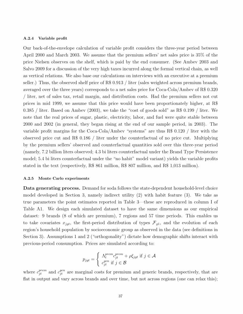
A.2.4 Variable profit
Our back-of-the-envelope calculation of variable profit considers the three-year period between
April 2000 and March 2003. We assume that the premium sellers’ net sales price is 35% of the
price Nielsen observes on the shelf, which is paid by the end consumer. (See Ambev 2003 and
Salvo 2009 for a discussion of the very high taxes incurred along the formal vertical chain, as well
as vertical relations. We also base our calculations on interviews with an executive at a premium
seller.) Thus, the observed shelf price of R$ 0.913 / liter (sales weighted across premium brands,
averaged over the three years) corresponds to a net sales price for Coca-Cola/Ambev of R$ 0.320
/ liter, net of sales tax, retail margin, and distribution costs. Had the premium sellers not cut
prices in mid 1999, we assume that this price would have been proportionately higher, at R$
0.385 / liter. Based on Ambev (2003), we take the “cost of goods sold” as R$ 0.199 / liter. We
note that the real prices of sugar, plastic, electricity, labor, and fuel were quite stable between
2000 and 2002 (in general, they began rising at the end of our sample period, in 2003). The
variable profit margins for the Coca-Cola/Ambev “systems” are thus R$ 0.120 / liter with the
observed price cut and R$ 0.186 / liter under the counterfactual of no price cut. Multiplying
by the premium sellers’ observed and counterfactual quantities sold over this three-year period
(namely, 7.2 billion liters observed; 4.3 bi liters counterfactual under the Brand Type Persistence
model; 5.4 bi liters counterfactual under the “no habit” model variant) yields the variable profits
stated in the text (respectively, R$ 861 million, R$ 807 million, and R$ 1,013 million).
A.2.5 Monte Carlo experiments
Data generating process. Demand for soda follows the state-dependent household-level choice
model developed in Section 3, namely indirect utility (2) with habit feature (3). We take as
true parameters the point estimates reported in Table 3—these are reproduced in column I of
Table A1. We design each simulated dataset to have the same dimensions as our empirical
dataset: 9 brands (8 of which are premium), 7 regions and 57 time periods. This enables us
to take covariates xjgt, the first-period distribution of types Fg1, and the evolution of each
region’s household population by socioeconomic group as observed in the data (see definitions in
Section 3). Assumptions 1 and 2 (“orthogonality”) dictate how demographic shifts interact with
previous-period consumption. Prices are simulated according to:
pjgt =
Λpremt cpremjt + ρξjgt if j ∈ A
cgenjt if j ∈ B
where cpremjt and cgenjt are marginal costs for premium and generic brands, respectively, that are
flat in output and vary across brands and over time, but not across regions (one can relax this);
37

Λpremt is a time-varying price markup over marginal cost for premium brands (this can also be
made to vary across brands and regions); unobserved taste shocks ξjgt are i.i.d. across brands
(including generics), regions and time; and 0 ≤ ρ < 1 is a pass-through ratio from utility shocks
for premium brands to prices. Define marginal costs as the time-varying price of inputs W
(e.g., sugar) times a cost efficiency (inverse productivity) parameter τ that varies by brand type
(premium or generic) and over time, plus a brand-and-time varying disturbance term u:
cpremjt = Wtτpremt + ujt
cgenjt = Wtτgent + ujt
Specifically, the simulations reported in Table A1—except column V—consider price variation
that is inspired by (is “comparable” to) what we observe in the real data: (i) premium brands’
markup Λpremt ∼ N(2, 0.022) until April-May 1999 and, following the 20% price cut, Λprem
t ∼N(1.6, 0.022) thereafter; (ii) factor price Wt ∼ U(0.85, 1.15); (iii) premium brands’ cost efficiency
τ premt equal to 0.55 throughout the sample period; (iv) generics’ cost efficiency τ gent equal to 0.9
in the first period, decreasing linearly to 0.6 in August 2000, and constant thereafter; and (v)
brand cost disturbance ujt ∼ N(0, 0.012).
By contrast, the simulation reported in column V, marked “less simulated data variation versus
real”: (i) drops the premium price cut, simulating the premium brands’ markup according to
Λpremt ∼ N(2, 0.022) throughout; (ii) drops the fringe’s price decline, setting the generics’ cost
efficiency τ gent already at 0.6 from the first period; and (iii) freezes each region’s household
population by socioeconomic group (EA,NA,P ) from the second period on.
Completing the description of the simulated datasets, we consider a pass-through ratio ρ = 0.3
and model utility shocks ξjgt ∼ N(0, σ2) with varying orders of magnitude of variance, as reported
in each column of Table A1. Notice that our experiments do not rely on the established firms
pricing optimally, and that premium prices are endogenous since the established firms pass
through a proportion of brand-market specific taste shocks to prices. Because taste shocks are
i.i.d. and prices correlate across regions through a common cost (and markup) structure, prices
in one region are a valid instrument for prices in another region.
Estimation. To estimate using simulated data, we follow the estimation procedure proposed
in Section 4. This includes adopting the same three instrument classes, namely: (i) the price of
inputs, (ii) the contemporaneous mean price for a brand in the other regions, and (iii) a dummy
variable indicating periods after July 1999 interacted with brand-region fixed effects. Since we
calculate household-type specific brand shares analytically, there is no sampling variation in
the logit shock εijgt. For every simulation ω = 1, ...,Ω, we complete the experimental—i.e.,
38

aggregate—dataset and make inference using the true (baseline) demand model (see columns II
to V). As in Section 5, we also estimate a no-habit model variant (column VI).
Results. With σ = 0.001, the estimated baseline model recovers the true parameters to at
least 2 decimal places (column II). Precision falls but is still quite high, particularly for λ, when
σ = 0.1 (column IV). Estimates using simulated data that exhibits less rich variation than what
we observe empirically—namely, where we shut down the premium price cut, the generic price
decline and the socioeconomic transitions—are substantially more noisy (column V compared to
column IV). Estimates using the no-habit model variant (column VI compared to column IV)
are noisier and, importantly, price sensitivity appears biased downward (for brevity, the bottom
of the table reports household-type specific elasticities for Coke only).
B Tables and Figures
Table 1: Brand Volume Shares of the Soda Category
Brand Region 1 Region 2 Region 3 Region 4 Region 5 Region 6 Region 7t=1 t=57 t=1 t=57 t=1 t=57 t=1 t=57 t=1 t=57 t=1 t=57 t=1 t=57
Coke 0.40 0.21 0.37 0.26 0.36 0.26 0.32 0.24 0.31 0.25 0.28 0.31 0.34 0.29Fanta 0.08 0.06 0.05 0.08 0.05 0.09 0.08 0.09 0.06 0.08 0.06 0.08 0.03 0.05Kuat 0.03 0.06 0.02 0.04 0.04 0.06 0.07 0.06 0.06 0.04 0.04 0.04 0.05 0.03Diet Coke 0.02 0.03 0.02 0.03 0.03 0.05 0.02 0.04 0.03 0.03 0.03 0.04 0.02 0.03Other Coca-Cola 0.02 0.03 0.02 0.02 0.02 0.02 0.05 0.06 0.04 0.05 0.05 0.04 0.05 0.02Guarana Antartica 0.17 0.09 0.07 0.06 0.06 0.09 0.09 0.10 0.08 0.07 0.05 0.05 0.09 0.10Other Ambev 0.19 0.02 0.11 0.01 0.15 0.01 0.16 0.02 0.12 0.01 0.17 0.01 0.06 0.02Pepsi 0.06 0.03 0.08 0.03 0.19 0.07 0.05 0.05 0.06 0.04 0.11 0.09 0.09 0.05Generics 0.03 0.47 0.26 0.47 0.12 0.36 0.17 0.34 0.25 0.41 0.21 0.33 0.27 0.41
Volume shares of the soda category, by brand in each region in the first and last time periods. Coke, Fanta, Kuat, Diet Coke, and“Other Coca-Cola” are premium brands marketed by the Coca-Cola Company. Guarana Antarctica, Pepsi, and “Other Ambev” arepremium brands marketed by Ambev. Source: Nielsen.
39

Table 2: Soda Consumption by Socioeconomic Group (HEX)Region of Socioeconomic Households ×1000 Soda By brand type Nosurvey. cities group Universe % purchasing Premium Generic soda
1 (Northeast) ABC 696 36 28.0% 27.0% 0.9% 72.0%DE 1230 64 9.1% 8.3% 0.8% 90.9%
2 (MG, ES, ABC 529 57 39.9% 37.9% 2.0% 60.1%RJ interior) DE 404 43 23.2% 22.1% 1.2% 76.8%3 (RJ Metro) ABC 1625 55 31.9% 31.6% 0.3% 68.1%
DE 1331 45 18.3% 18.3% 0.0% 81.7%4 (SP Metro) ABC 2586 60 34.5% 33.1% 1.4% 65.5%
DE 1689 40 19.8% 17.3% 2.6% 80.2%6 (South) ABC 955 63 43.2% 42.5% 0.7% 56.8%
DE 559 37 20.4% 20.1% 0.3% 79.6%7 (DF, GO ABC 428 61 36.5% 34.4% 2.1% 63.5%MS) DE 270 39 23.6% 21.1% 2.5% 76.4%
The extensive margin of soda consumption inside the home by different socioeconomic groups in 1995/96. Socioeconomic groups aredefined per the points scale used by IBOPE. Metropolitan areas surveyed were: (Region 1) Recife, Fortaleza and Salvador; (Region2) Belo Horizonte; (Region 3) Rio de Janeiro Metro; (Region 4) Sao Paulo Metro; (Region 6) Curitiba and Porto Alegre; (Region 7)Brasilia and Goiania. No city was surveyed in Region 5 (state of Sao Paulo excluding Sao Paulo Metro). We do not consider thenorthern city of Belem as it is located outside the area covered by Nielsen. Source: IBGE HEX 1995/96.
Table 3: Demand Estimation Results
coeff (s.e.) coeff (s.e.) coeff (s.e.)Price Sensitivity Parameters CombinationsαEA 3.56 (1.39) α+ αEA -2.14 (0.17)αNA 1.80 (1.42) α+ αNA -3.90 (0.61)α -5.70 (1.43) αEA − αNA 1.76 (0.52)
Habit Parameterλ 4.20 (0.26)
Other EffectsConstant -3.84 (0.37)Temperature 2.91 (0.32)
Advertising GRPs: In-store Presence: Time Trends:Advertising×Region 1 0.44 (0.22) Distribution×Region 1 3.10 (0.27) Region 1 -0.37 (0.12)Advertising×Region 2 0.25 (0.37) Distribution×Region 2 3.70 (0.46) Region 2 0.13 (0.19)Advertising×Region 3 0.00 (0.27) Distribution×Region 3 4.09 (0.96) Region 3 -0.33 (0.12)Advertising×Region 4 0.40 (0.37) Distribution×Region 4 2.72 (0.45) Region 4 -0.66 (0.09)Advertising×Region 5 0.32 (0.32) Distribution×Region 5 3.33 (0.48) Region 5 0.02 (0.17)Advertising×Region 6 0.66 (0.34) Distribution×Region 6 1.24 (0.28) Region 6 -0.05 (0.17)Advertising×Region 7 0.49 (0.32) Distribution×Region 7 1.11 (0.33) Region 7 -0.07 (0.21)
Seasonality×Brand Type Effects YesBrand-Region Fixed Effects Yes
Standard errors in parentheses. Source: estimated baseline model.
40

Table 4: Estimated Demand Elasticities
Aggregate Own-Price Elasticities Household-Type Specific Own-Price Elasticities
Coke -1.65 Coke, EAA -1.42 Generic, EAA -1.33Guarana Antarctica -2.06 Coke, EAB -2.29 Generic, EAB -0.23Fanta -2.01 Coke, EAO -2.18 Generic, EAO -1.24Pepsi -2.01 Coke, NAA -3.29 Generic, NAA -2.42Generic -0.68 Coke, NAB -4.20 Generic, NAB -0.86
Coke, NAO -4.16 Generic, NAO -2.37Coke, PA -5.70 Generic, PA -3.56Coke, PB -6.14 Generic, PB -2.14Coke, PO -6.14 Generic, PO -3.54
Reported elasticities are means across region-and-time markets, and only a few elasticities are shown due to space constraints.
Table 5: Predicted Consumption Patterns and Habit Transitions by Type
A: Predicted Soda Penetration and Consumption Patterns by Socioeconomic Group*
Soda Penetration Premium Share Generic Share Generic:Premium RatioEstablished Affluent 0.69 0.47 0.23 0.5Newly Affluent 0.22 0.09 0.13 1.4Poor 0.05 0.01 0.04 2.7
*Soda penetration, for the entire category and by type of brand, in each socioeconomic group, as predicted bythe estimated demand model. Reported numbers are means across all regions over the last 12 months of the sample.
B: Transitions by Household Type**
Premium Habit Generic Habit No HabitEAA 0.90 0.01 0.09EAB 0.02 0.87 0.11EAO 0.15 0.09 0.76NAA 0.66 0.01 0.33NAB 0.01 0.73 0.26NAO 0.04 0.04 0.92PA 0.31 0.01 0.68PB 0.00 0.52 0.48PO 0.01 0.02 0.97
** Reported transition rates are means across all regions in the last 12 months of the sample.
41

Table 6: Estimates from the “No Habit” Demand Model
coeff (s.e.) coeff (s.e.)Price Sensitivity Parameters
Parameter Combinations:αEA 0.47 (0.58) α+ αEA -1.51 (0.19)αNA -0.85 (0.35) α+ αNA -2.83 (0.65)α -1.98 (0.42) αEA − αNA 1.32 (0.77)
Other EffectsConstant -2.72 (0.24)Temperature 1.64 (0.11)
Advertising×Region YesIn-store Presence×Region YesTime Trend×Region YesSeasonality×Brand Type Effects YesBrand-Region Fixed Effects Yes
Table A1: Monte Carlo Experiments
I II III IV V VIModel Baseline Baseline Baseline Baseline No-habitSimulated vs. actual ”Comparable” ”Comparable” ”Comparable” ”Less” ”Comparable”σ 0.001 0.01 0.1 0.1 0.1
True Median (S.D.) Median (S.D.) Median (S.D.) Median (S.D.) Median (S.D.)
Price SensitivityαEA 3.56 3.56 (0.00) 3.57 (0.04) 3.55 (0.38) 3.20 (0.71) 3.50 (1.13)αNA 1.80 1.80 (0.00) 1.80 (0.04) 1.80 (0.37) 0.67 (23.80) 2.94 (1.03)α -5.70 -5.70 (0.00) -5.71 (0.04) -5.66 (0.42) -5.24 (0.65) -4.96 (1.19)
Combinations:α+ αEA -2.14 -2.14 (0.00) -2.14 (0.01) -2.09 (0.06) -2.04 (0.14) -1.45 (0.07)α+ αNA -3.90 -3.90 (0.00) -3.90 (0.01) -3.85 (0.14) -4.34 (23.82) -2.01 (0.21)αEA − αNA 1.76 1.76 (0.00) 1.76 (0.01) 1.76 (0.10) 2.27 (23.83) 0.56 (0.16)
Habitλ 4.20 4.20 (0.00) 4.20 (0.01) 4.16 (0.09) 4.18 (0.15) – –
Household-Type Specific Own-Price Elasticities for Coke
EAA -1.08 (0.02) -1.08 (0.02) -1.06 (0.03) -1.25 (0.11) -1.22 (0.06)EAB -1.99 (0.02) -1.99 (0.03) -1.94 (0.06) -2.24 (0.15) -1.22 (0.06)EAO -1.87 (0.03) -1.87 (0.03) -1.83 (0.05) -2.14 (0.16) -1.22 (0.06)NAA -2.46 (0.05) -2.47 (0.05) -2.44 (0.13) -3.85 (26.60) -1.74 (0.19)NAB -3.64 (0.05) -3.64 (0.05) -3.60 (0.13) -4.76 (26.18) -1.74 (0.19)NAO -3.60 (0.05) -3.60 (0.05) -3.56 (0.13) -4.75 (26.20) -1.74 (0.19)PA -4.58 (0.09) -4.58 (0.11) -4.58 (0.52) -5.15 (0.83) -4.52 (1.14)PB -5.34 (0.07) -5.35 (0.08) -5.32 (0.40) -5.71 (0.71) -4.52 (1.14)PO -5.33 (0.07) -5.34 (0.08) -5.31 (0.41) -5.71 (0.72) -4.52 (1.14)
Medians and standard deviations (in parentheses) of estimated parameters are taken over 50 simulations (reported standard devia-tions in column VI exclude one iteration, ω = 24, for which estimates were clear outliers). Reported elasticities are means acrossregion-and-time markets.
42

Figure 1: The evolution of quantities (in million liters/month) by type of brand (Premium versus Generic), for soda sold in family-size bottles through the self-service channel across the seven Nielsen regions, in the period Dec-96 to Mar-03. Source: Nielsen.
0 10 20 30 40 50 60 70 800
50
100
150
200
250
300Monthly Premium & Generic Quantities Sold, sums across 7 regions
Months since November 1996
Mill
ion
liter
s pe
r mon
th
Premium volumeGeneric volume
0 10 20 30 40 50 60 70 800.1
0.2
0.3
0.4
0.5
0.6
0.7
0.8
0.9Premium & Generic Volume Shares of Soda Category across 7 regions
Months since November 1996
Vol
ume
Sha
res
of S
oda
Cat
egor
y
Premium shareGeneric share
0 10 20 30 40 50 60 70 800.5
0.6
0.7
0.8
0.9
1
1.1
1.2
1.3Share-Weighted Premium & Generic Prices, means across 7 regions
Months since November 1996
Sha
re-w
eigh
ted
pric
e
Premium priceGeneric price
Figure 2: The evolution of prices (in constant Brazilian R$/liter) and category volume shares (in percent, summing to one) by type of brand (Premium versus Generic), for soda sold in family-size bottles through the self-service channel across the seven Nielsen regions, in the period Dec-96 to Mar-03. Source: Nielsen.
May 1999 May 1999
43

120
130
140
150
160
170
180
190
200
30
35
40
45
50
55
60
65
70
75
1986 1988 1990 1992 1994 1996 1998 2000 2002 2004 2006An
nual
per
-cap
ita (b
agge
d) c
emen
t con
sum
ptio
n
Annu
al p
er-c
apita
soda
con
sum
ptio
n
year
soda (liters per capita) cement (kg per capita)
Figure 3: Annual aggregate per capita consumption of soft drinks (in liters per person) and of bagged cement (in kilograms per person). (Cement sold in bags, as opposed to sales in bulk, filter out any large-scale construction activity, such as government spending on infrastructure.) Sources: Brazilian trade associations for soft drink makers and for cement producers, ABIR and SNIC respectively.
Real stabilization plan (July 1994)
44

0%10%
20%
30%
40%
50%
60%
70%
80%
90%
100%
time
Regi
on 4
(met
ropo
litan
are
a of
SP
city
)
% P
oor
% N
ewly
Aff
luen
t%
Est
ablis
hed
Afflu
ent
0%10%
20%
30%
40%
50%
60%
70%
80%
90%
100%
tim
e
Regi
on 5
(sta
te o
f SP
excl
udin
g m
etro
polit
an a
rea
of S
P ci
ty)
% P
oor
% N
ewly
Aff
luen
t%
Est
ablis
hed
Afflu
ent
0%10%
20%
30%
40%
50%
60%
70%
80%
90%
100%
tim
e
Regi
on 6
(sta
tes
in th
e So
uth)
% P
oor
% N
ewly
Aff
luen
t%
Est
ablis
hed
Afflu
ent
0%10%
20%
30%
40%
50%
60%
70%
80%
90%
100%
time
Regi
on 1
(sta
tes i
n th
e N
orth
east
exc
ludi
ng M
A an
d PI
)
% P
oor
% N
ewly
Aff
luen
t%
Est
ablis
hed
Afflu
ent
0%10%
20%
30%
40%
50%
60%
70%
80%
90%
100%
tim
e
Regi
on 2
(sta
tes o
f MG
, ES
and
RJ e
xcl.
the
met
rop.
are
a of
RJ c
ity)
% P
oor
% N
ewly
Aff
luen
t%
Est
ablis
hed
Afflu
ent
0%10%
20%
30%
40%
50%
60%
70%
80%
90%
100%
tim
e
Regi
on 3
(met
ropo
litan
are
a of
RJ c
ity)
% P
oor
% N
ewly
Aff
luen
t%
Est
ablis
hed
Afflu
ent
Figu
re 4
: The
rise
of “
new
ly a
fflue
nt”
hous
ehol
ds: P
ropo
rtio
n of
urb
an h
ouse
hold
s in
eac
h of
thre
e co
nstr
ucte
d so
cioe
cono
mic
gro
ups
(“Es
tabl
ishe
d A
fflue
nt,”
“N
ewly
Affl
uent
” an
d “P
oor”
), as
def
ined
in
the
text
, by
regi
on in
the
peri
od D
ec-9
6 to
Mar
-03.
The
sm
alle
st re
gion
by
num
ber o
f hou
seho
lds,
reg
ion
7 (F
eder
al D
istr
ict a
nd s
tate
s of G
O a
nd M
S), i
s not
sho
wn
for l
ack
of s
pace
(the
pat
tern
is si
mila
r to
regi
on 2
). So
urce
s: IB
OPE
Lat
inPa
nel,
IBG
E PN
AD
.
45

0 2 4 6 8 10 12 14 16 18 20 22 24 26 28 30 32 34 36 38 40 42 44 46 48 50 52 54 56 58 60 62 64 66 68 70 72 74 76 78-8
-7
-6
-5
-4
-3
-2
-1Household-type-specific own-price elasticities for Coke brand in Region 4
Months since November 1996
Ow
n el
astic
ity
EstablAffl-PremiumEstablAffl-GenericEstablAffl-NoSodaNewAffl-PremiumNewAffl-GenericNewAffl-NoSodaPoor-PremiumPoor-GenericPoor-NoSoda
Figure 5: Evolution of own-price elasticities for Coke brand (left panel) and Generics (right panel), by household type, in region 4 (São Paulo Metro). Source: baseline model.
0 2 4 6 8 10 12 14 16 18 20 22 24 26 28 30 32 34 36 38 40 42 44 46 48 50 52 54 56 58 60 62 64 66 68 70 72 74 76 78-4.5
-4
-3.5
-3
-2.5
-2
-1.5
-1
-0.5
0Household-type-specific own-price elasticities for Generics in Region 4
Months since November 1996
Ow
n el
astic
ity
EstablAffl-PremiumEstablAffl-GenericEstablAffl-NoSodaNewAffl-PremiumNewAffl-GenericNewAffl-NoSodaPoor-PremiumPoor-GenericPoor-NoSoda
46
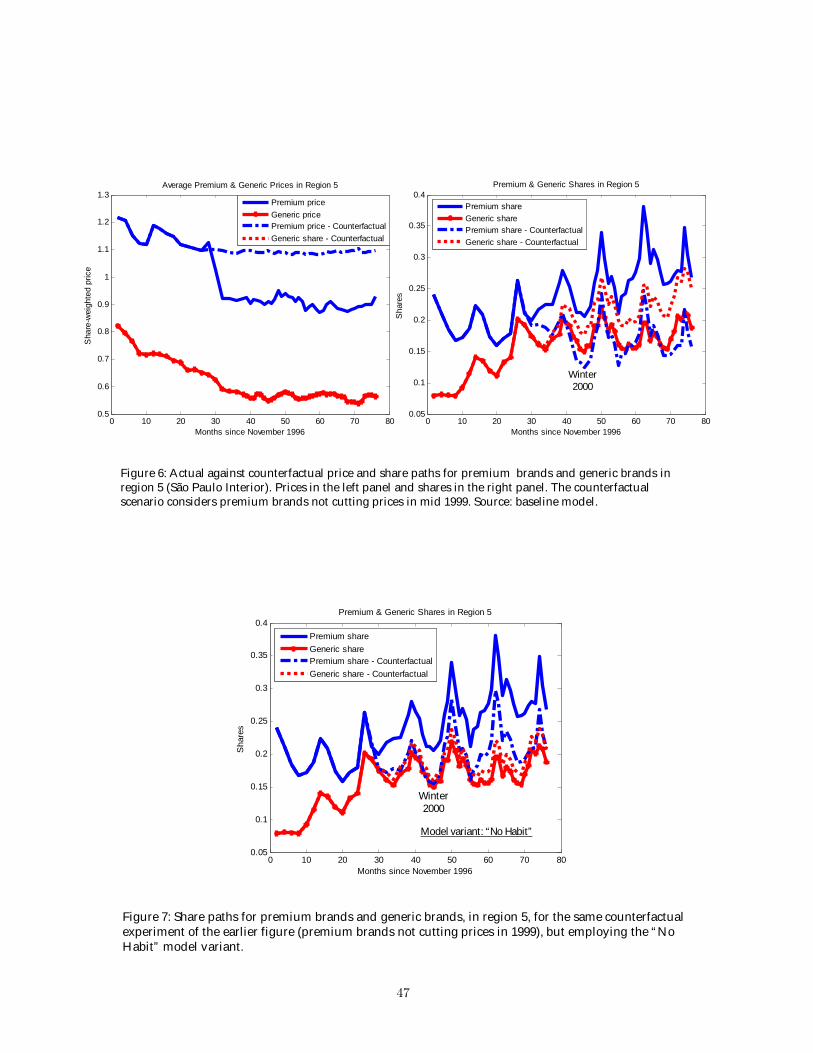
0 10 20 30 40 50 60 70 800.5
0.6
0.7
0.8
0.9
1
1.1
1.2
1.3Average Premium & Generic Prices in Region 5
Months since November 1996
Sha
re-w
eigh
ted
pric
e
Premium priceGeneric pricePremium price - CounterfactualGeneric share - Counterfactual
0 10 20 30 40 50 60 70 800.05
0.1
0.15
0.2
0.25
0.3
0.35
0.4Premium & Generic Shares in Region 5
Months since November 1996
Sha
res
Premium shareGeneric sharePremium share - CounterfactualGeneric share - Counterfactual
Figure 6: Actual against counterfactual price and share paths for premium brands and generic brands in region 5 (São Paulo Interior). Prices in the left panel and shares in the right panel. The counterfactual scenario considers premium brands not cutting prices in mid 1999. Source: baseline model.
Winter 2000
0 10 20 30 40 50 60 70 800.05
0.1
0.15
0.2
0.25
0.3
0.35
0.4Premium & Generic Shares in Region 5
Months since November 1996
Sha
res
Premium shareGeneric sharePremium share - CounterfactualGeneric share - Counterfactual
Figure 7: Share paths for premium brands and generic brands, in region 5, for the same counterfactual experiment of the earlier figure (premium brands not cutting prices in 1999), but employing the “No Habit” model variant.
Model variant: “No Habit”
Winter2000
47

Figure A1: The evolution of premium soda media advertising intensity (in monthly Gross Rating Points, GRP, ×1000) and the proportions of stores with specific brands in stock (in percent), in the period Dec-96 to Mar-03. GRP and percentages shown are means across the seven Nielsen regions. Sources: McCann-Erickson, Nielsen.
0 10 20 30 40 50 60 70 802
4
6
8
10
12
14
16
18
20
22Premium Soda Advertising Intensity, means across 7 regions
Months since November 1996
GR
P X
100
0 su
mm
ed o
ver b
rand
s
Premium brands
0 10 20 30 40 50 60 70 800
10
20
30
40
50
60
70
80
90
100Distribution of Coke and generics, means across 7 regions
Months since November 1996
Per
cent
of s
tore
s
Coke brand on shelfGenerics on shelf
48