GPUs Immediately Relating Lattice QCD to Collider Experiments

GTC 2013 | Dr. Mathias Wagner | Bielefeld University |

GPUs Immediately Relating Lattice QCD to Collider Experiments


Outline•Quantum ChromoDynamics

•Fluctuations from Heavy-Ion experiments and lattice QCD

•Lattice QCD on GPUs and on the Bielefeld GPU cluster

•Optimizations

• includes first experiences with Kepler architecture

•Relating Lattice Data to Collider Experiments

•Outlook


Outline•Quantum ChromoDynamics

•Fluctuations from Heavy-Ion experiments and lattice QCD

•Lattice QCD on GPUs and on the Bielefeld GPU cluster

•Optimizations

• includes first experiences with Kepler architecture

•Relating Lattice Data to Collider Experiments

•Outlook

→ Lattice-QCD talks by: Frank Winter ( Wed, 10:00 ) Balint Joo ( Wed,10:30 ) Hyung-Jin Kim ( Thu,16:30 )

→ Lattice-QCD posters: Hyung-Jin Kim Richard Forster Alexei Strelchenko


Strong force

3(8)The Nobel Prize in Physics 2008 The Royal Swedish Academy of Sciences www.kva.se

seen before. Most of them did not fi t into the models physicists had at that time, that matter consisted of atoms with neutrons and protons in the nucleus and electrons round it. Deeper investigations into the innermost regions of matter revealed that protons and neutrons each concealed a trio of quarks. The particles that had already been discovered also were shown to consist of quarks.

Now, almost all the pieces of the puzzle have fallen into place; a Standard Model for the indivisible parts of matter comprises three families of particles (see diagram). These fami-lies resemble each other, but only the particles in the fi rst and lightest family are suffi ciently stable to build up the cosmos. The particles in the two heavier families live under very unsta-ble conditions and disintegrate immediately into lighter kinds of particles.

Everything is controlled by forces. The Standard Model, at least for the time being, includes three of nature’s four fundamental forces along with their messengers, particles that convey the interaction between the elementary particles (see diagram). The messenger of the electromagne-tic force is the photon with zero mass; the weak force that accounts for radioactive disintegration and causes the sun and the stars to shine is carried by the heavy W and Z boson particles; while the strong force is carried by gluon particles, which see to it that the atom nuclei hold together. Gravity, the fourth force, which makes sure we keep our feet on the ground, has not yet been incorporated into the model and poses a colossal challenge for physicists today.

The mirror is shattered

The Standard Model is a synthesis of all the insights into the innermost parts of matter that physics has gathered during the last century. It stands fi rmly on a theoretical base consisting

Molecule Atom nucleus Proton/neutronAtom Quark

Into the matter. Electrons and quarks are the smallest building blocks of all matter.

The Standard Model today. It unifi es all the fundamental building blocks of matter and three of the four fundamental forces. While all known matter is built with particles from the fi rst family, the other particles exists but only for extremely short time periods. To complete the Model a new particle is needed – the Higgs particle – that the physics community hopes to fi nd in the new built accelerator LHC at CERN in Geneva.

Elementary particlesFirst family Second family Third family

electronneutrino

muonneutrino

tauneutrino

electron muon tau

up

Qua

rks

Lept

ons

charm

down strange bottom

topweak force

electromagnetic force

W, Z

photon

gluons

Forces Messenger particles

strong force

Higgs?

•acts on quarks

•force carriers: gluons(c.f. electrodynamics: photons)

•range:

•strength: times stronger than gravity times stronger than electromagnetism

•residual interaction: nuclear force (i.e. force between nuclei in atom nucleus)

•described by Quantum ChromoDynamics (QCD)

1015 m

1038

102


Phase transitions

•water at different temperatures

•ice (solid)

•water (liquid)

•vapor (gas)

•phase transitions occur in different ways: 1st order, 2nd order, ‘crossover’

•a ‘order parameter’ describes the change between different states

•boiling point of water depends on pressure → phase diagram


Phase transitions

•water at different temperatures

•ice (solid)

•water (liquid)

•vapor (gas)

•phase transitions occur in different ways: 1st order, 2nd order, ‘crossover’

•a ‘order parameter’ describes the change between different states

•boiling point of water depends on pressure → phase diagram

arX

iv:0

801.

4256

v2 [

hep-

ph]

28 Ju

l 200

9

The Phase Diagram of Strongly Interacting Matter

P. Braun-Munzinger1, 2 and J. Wambach1, 2

1GSI Helmholtzzentrum fur Schwerionenforschung mbH, Planckstr, 1, D64291 Darmstadt, Germany2Technical University Darmstadt, Schlossgartenstr. 9, D64287 Darmstadt, Germany

A fundamental question of physics is what ultimately happens to matter as it is heated or com-pressed. In the realm of very high temperature and density the fundamental degrees of freedom ofthe strong interaction, quarks and gluons, come into play and a transition from matter consistingof confined baryons and mesons to a state with ’liberated’ quarks and gluons is expected. Thestudy of the possible phases of strongly interacting matter is at the focus of many research activi-ties worldwide. In this article we discuss physical aspects of the phase diagram, its relation to theevolution of the early universe as well as the inner core of neutron stars. We also summarize recentprogress in the experimental study of hadronic or quark-gluon matter under extreme conditionswith ultrarelativistic nucleus-nucleus collisions.

PACS numbers: 21.60.Cs,24.60.Lz,21.10.Hw,24.60.Ky

Contents

I. Introduction 1

II. Strongly Interacting Matter under ExtremeConditions 2A. Quantum Chromodynamics 2B. Models of the phase diagram 4

III. Results from Lattice QCD 7

IV. Experiments with Heavy Ions 8A. Opaque fireballs and the ideal liquid scenario 9B. Hadro-Chemistry 10C. Medium modifications of vector mesons 12D. Quarkonia–messengers of deconfinement 15

V. Phases at High Baryon Density 17A. Color Superconductivity 17

VI. Summary and Conclusions 18

Acknowledgments 19

References 19

I. INTRODUCTION

Matter that surrounds us comes in a variety of phaseswhich can be transformed into each other by a change ofexternal conditions such as temperature, pressure, com-position etc. Transitions from one phase to another areoften accompanied by drastic changes in the physicalproperties of a material, such as its elastic properties,light transmission, or electrical conductivity. A good ex-ample is water whose phases are (partly) accessible toeveryday experience. Changes in external pressure andtemperature result in a rich phase diagram which, be-sides the familiar liquid and gaseous phases, features avariety of solid (ice) phases in which the H20 moleculesarrange themselves in spatial lattices of certain symme-tries (Fig. 1).

Twelve of such crystalline (ice) phases are known atpresent. In addition, three amorphous (glass) phases

FIG. 1 The phase diagram of H20 (Chaplin, 2007). Be-sides the liquid and gaseous phases a variety of crystallineand amorphous phases occur. Of special importance in thecontext of strongly interacting matter is the critical endpointbetween the vapor and liquid phase.

have been identified. Famous points in the phase dia-gram are the triple point where the solid, liquid, and gasphases coexist and the critical endpoint at which there isno distinction between the liquid and gas phase. This isthe endpoint of a line of first-order liquid-gas transitions;at this point the transition is of second order.

Under sufficient heating water and, for that matter anyother substance, goes over into a new state, a ’plasma’,consisting of ions and free electrons. This transitionis mediated by molecular or atomic collisions. It iscontinuous 1 and hence not a phase transition in thestrict thermodynamic sense. On the other hand, the

1 Under certain conditions there may also be a true plasma phasetransition, for recent evidence see (Fortov et al., 2007).


Phases of Quantum ChromDynamics

•extreme conditions (temperatures, densities) are necessary to investigate properties of QCD

•important for understanding the evolution of the universe after the Big Bang

hadron gas dense hadronic matter quark gluon plasma

cold hot

cold nuclear matter phase transition or quarks and gluons areQuarks and gluons are crossover at Tc the degrees of freedomconfined inside hadrons (asymptotically) free


Accelerators ... the real ones

LHC @ CERN RHIC @ Brookhaven National Lab


Heavy Ion Experiments

•phase transition occurs in heavy-ion collisions

•What thermometer can we use at ?

•detectors measure created particles

•to interpret the data theoretical input is required

•ab-initio approach: Lattice QCD

Heavy Ion Collision QGP Expansion+Cooling Hadronization

1012 K


Heavy Ion Experiments

•phase transition occurs in heavy-ion collisions

•What thermometer can we use at ?

•detectors measure created particles

•to interpret the data theoretical input is required

•ab-initio approach: Lattice QCD

Heavy Ion Collision QGP Expansion+Cooling Hadronization GPUs used for triggering and data processing→ Valerie Halyo (Wed, 16.30) S3263 Alessandro Lonardo (Wed, 15.30) S3286

F. Pantaleo & V. Innocente (Wed, 16.00) S3278

1012 K


Lattice QCD

•QCD partition function

•4 dimensional grid (=Lattice)

•quarks live on lattice sites

•6 or 12 complex numbers

•gluons live on the links

•SU(3) matrices

•18 complex numbers

•typical sizes: 24 x 24 x 24 x 6 to 256 x 256 x 256 x 256

Formulating Lattice QCD

• Quark fields live on the lattice sites

• “spinors”

• 12 complex numbers

• Gluon fields live on the links

• SU(3) “Color matrices”

• 18 complex numbers

Friday, 11 March 2011

ZQCD (T, µ) =

ZDADDeSE(T,µ)

includes integral over space and time


Fluctuations and the QCD phase diagram

•different QCD phases characterized by

•chiral symmetry

•confinement aspects

Figure from C. Schmidt

T [

GeV

] QCD

hadron gas

nuclear matterneutron stars

0

vacuum

quark-gluon-plasma0.16

chemical potential µB

critical end-point


Fluctuations and the QCD phase diagram

•different QCD phases characterized by

•chiral symmetry

•confinement aspects

•possible critical end-point

•2nd order phase transition

•divergent correlation length

•divergent susceptibility


T [

GeV

] QCD

hadron gas


0

vacuum

quark-gluon-plasma0.16

chemical potential µB

critical end-point


Fluctuations from Lattice QCD•expansion of the pressure in

•B,Q,S conserved charges (baryon number, electric charge, strangeness)

p

T 4=

1X

i,j,k

1

i!j!k!BQSijk

µB

T

i µQ

T

j µS

T

k




•generalized susceptibilities

p

T 4=

1X

i,j,k

1

i!j!k!BQSijk

µB

T

i µQ

T

j µS

T

k

BQSijk =

1

V T

@i

@(µB/T )

@j

@(µQ/T )

@k

@(µS/T )Z(T, µ)

µ=0




•generalized susceptibilities

•related to cumulants of net charge fluctuations, e.g.

p

T 4=

1X

i,j,k

1

i!j!k!BQSijk

µB

T

i µQ

T

j µS

T

k

BQSijk =

1

V T

@i

@(µB/T )

@j

@(µQ/T )

@k

@(µS/T )Z(T, µ)

µ=0

V T 3B2 = h(NB)

2i =N2

B 2NBhNBi+ hNBi2↵


Calculation of susceptibilities from Lattice QCD

•µ-dependence is contained in the fermion determinant

•calculation of susceptibilities requires µ-derivatives of fermion determinant

Z =

ZDU(detM(µ))Nf/4

exp(Sg),

@2 lnZ@µ2

=

nf

4

@2(ln detM)

@µ2

+

*nf

4

@(ln detM)

@µ

2+


Calculation of susceptibilities from Lattice QCD

•µ-dependence is contained in the fermion determinant

•calculation of susceptibilities requires µ-derivatives of fermion determinant

•formulate all operator in terms of traces over space-time, color (and spin)

•full inversion of fermion matrix is impossible: evaluate using noisy estimators

•ensemble average → large number of configurations

Z =

ZDU(detM(µ))Nf/4

exp(Sg),

@2 lnZ@µ2

=

nf

4

@2(ln detM)

@µ2

+

*nf

4

@(ln detM)

@µ

2+


Noisy estimators

•traces required for derivatives

•noisy estimators → large number of random vectors η (~1500 / configuration)

•up to 10000 configurations for each temperature

•dominant operation: fermion matrix inversion (~ 99%)

@(ln detM)

@µ=Tr

M1 @M

@µ

@2(ln detM)

@µ2=Tr

M1 @

2M

@µ2

Tr

M1 @M

@µM1 @M

@µ

...

Tr

@n1M

@µn1M1 @

n2M

@µn2. . .M1

= lim

N!1

1

N

NX

k=1

†k@n1M

@µn1M1 @

n2M

@µn2. . .M1k


Configuration generation

•sequential process

•use RHMC algorithm to evaluate the system in simulation time

Steps in a Lattice QCD calculation

1. Generate an ensemble of gluon field configurations,

2. Compute quark propagators in these fixed backgrounds by solving the Dirac equation for various right-hand sides

!"#$%&'()*$+%",-"#$.#(/01,(-23$$4$$5678$95:;;$$4$$8&1)*$;<$=>;; ?

!"#$%&'(&)&*)""'+#&,-.&+)*+/*)"'0(

;@$A0#01&-0$&#$0#,0B'C0$"D$ECF"#$D(0CG$)"#D(EF1&-("#,<

=@$9"BHF-0$IF&1J$H1"H&E&-"1,$(#$-*0,0$D(K0G$'&)JE1"F#G,$'2$,"C/(#E$-*0$L(1&)$0IF&-("#$D"1$/&1("F,$1(E*-M*&#G$,(G0,@

"1$N7KO'P

!"#$%&'()*$+%",-"#$.#(/01,(-23$$4$$5678$95:;;$$4$$8&1)*$;<$=>;; ?

!"#$%&'(&)&*)""'+#&,-.&+)*+/*)"'0(

;@$A0#01&-0$&#$0#,0B'C0$"D$ECF"#$D(0CG$)"#D(EF1&-("#,<


"1$N7KO'P!"#$%&'()*$+%",-"#$.#(/01,(-23$$4$$5678$95:;;$$4$$8&1)*$;<$=>;; ?

!"#$%&'(&)&*)""'+#&,-.&+)*+/*)"'0(

;@$A0#01&-0$&#$0#,0B'C0$"D$ECF"#$D(0CG$)"#D(EF1&-("#,<


"1$N7KO'P


P = @H

@Q= @S

@Q=

@Sg

@Q+

@Sf

@Q

Q =

@H

@P= P


Configuration generation

•sequential process

•use RHMC algorithm to evaluate the system in simulation time

•two dominant parts of the calculation (90% of the runtime)

•fermion force~50% for improved actions (HISQ)

•fermion matrix inversion~90% for standard action

Steps in a Lattice QCD calculation

1. Generate an ensemble of gluon field configurations,

2. Compute quark propagators in these fixed backgrounds by solving the Dirac equation for various right-hand sides

!"#$%&'()*$+%",-"#$.#(/01,(-23$$4$$5678$95:;;$$4$$8&1)*$;<$=>;; ?

!"#$%&'(&)&*)""'+#&,-.&+)*+/*)"'0(

;@$A0#01&-0$&#$0#,0B'C0$"D$ECF"#$D(0CG$)"#D(EF1&-("#,<


"1$N7KO'P

!"#$%&'()*$+%",-"#$.#(/01,(-23$$4$$5678$95:;;$$4$$8&1)*$;<$=>;; ?

!"#$%&'(&)&*)""'+#&,-.&+)*+/*)"'0(

;@$A0#01&-0$&#$0#,0B'C0$"D$ECF"#$D(0CG$)"#D(EF1&-("#,<


"1$N7KO'P!"#$%&'()*$+%",-"#$.#(/01,(-23$$4$$5678$95:;;$$4$$8&1)*$;<$=>;; ?

!"#$%&'(&)&*)""'+#&,-.&+)*+/*)"'0(

;@$A0#01&-0$&#$0#,0B'C0$"D$ECF"#$D(0CG$)"#D(EF1&-("#,<


"1$N7KO'P


P = @H

@Q= @S

@Q=

@Sg

@Q+

@Sf

@Q

Q =

@H

@P= P

Dynamical Simulations with Highly Improved Staggered Quarks R. M. Woloshyn

Figure 1: Paths used in the ASQTAD and HISQ actions. Path coefficients for ASQTAD can be foundin Ref. [4]. The HISQ effective links are constructed by first applying a Fat7 fattening to the baselinks (U →UF with coefficients 1-link:1/8, 3-staple:1/16, 5-staple:1/64, 7-staple:1/384), then a SU(3)-projection (UF → UR), and finally an “ASQ” smearing (UR → Uef f with coefficients 1-link:1+ ε/8, 3-staple:1/16, 5-staple:1/64, 7-staple:1/384, Lepage:−1/8, Naik:−(1+ ε)/24, where the parameter ε is in-troduced to remove (am)4 errors [9]).

The pseudo-fermion field Φ is defined on even lattice sites only to avoid a doubling of flavors fromusing M†M instead of M in the action. This procedure is valid since M†M has no matrix elementconnecting even and odd lattice sites.

A key component in dynamical simulations using molecular dynamics evolution is the com-putation of fermion force — derivative of the fermion action with respect to the base links

fx,µ =∂Sf∂Ux,µ

=∂

∂Ux,µ

⟨

Φ∣

∣

∣

[

M†[U ]M[U ]]−nf /4

∣

∣

∣Φ⟩

. (2.3)

The derivative can be computed straightforwardly if nf is a multiple of 4; for other numbers offermion flavors the 4th-root of M†M can be approximated by a rational expansion (the RHMCalgorithm [17, 18, 19])

[M†M]−nf /4 ≈ α0+∑l

αlM†M+βl

, (2.4)

where αl and βl are constants. The derivative becomes

∂Sf∂Ux,µ

= −∑lαl

⟨

Φ[M†M+βl]−1∣

∣

∣

∣

∂∂Ux,µ

(

M†[U ]M[U ])

∣

∣

∣

∣

[M†M+βl]−1Φ

⟩

= −∑lαl

(⟨

Xl∣

∣

∣

∣

∂D†[U ]

∂Ux,µ

∣

∣

∣

∣

Y l⟩

+

⟨

Y l∣

∣

∣

∣

∂D[U ]

∂Ux,µ

∣

∣

∣

∣

Xl⟩)

, (2.5)

with |Xl〉 = [M†M+βl]−1|Φ〉 and |Y l〉 = D|Xl〉. Note that Xl and Y l are defined on even and oddsites respectively. Taking the derivatives of D, D† with respect to Uef f , Uef f† and writing out thematrix indices we have

[

fx,µ]

ab =∂Sf

∂[

Ux,µ]

ab=∑

y,ν(−1)yηy,ν

(

∂ [Uef fy,ν ]mn

∂ [Ux,µ ]ab

[

f (0)y,ν

]

mn+∂ [Uef f†

y,ν ]mn∂ [Ux,µ ]ab

[

f (0)†y,ν

]

mn

)

, (2.6)

where f (0)y,ν is the vector outer product of the field variables at y and y+ν

[

f (0)y,ν

]

mn=

∑lαl[Y ly+ν ]n[X

l∗y ]m for even y

∑lαl[Xl

y+ν ]n[Yl∗y ]m for odd y

, (2.7)

3


History of QCD Machines in BI: the APE generation

• APE = Array Processor Experiment, started mid eigthties

• SIMD architecture with lot of FPUs, VLIW

• special purpose machine build for lattice QCD

• optimized a x b + c operation for use in complex matrix-vector multiplication

• large register files - up to 512 64bit-registers

• 3D network low latency: fast memory access to nearest neighbor (~ 3-4 local)

• low power consumption (latest version: ~ 1.5 GFlops @ 7 Watt)

• object-oriented programming language TAO (syntax similar to Fortran)

• controlled by host PC

2 CHEP03, La Jolla, California, March 24th-28th, 2003

Figure 1: One of the original 1988 APE boards.

which are specifically optimized for their applications.In this paper we describe the Array Processor Exper-iment (APE) project, which was started in the mideighties by the Istituto Nazionale di Fisica Nucleare(INFN) and is now carried out within the frameworkof a European collaboration with DESY and the Uni-versity of Paris Sud.

The structure of this paper is as follows: in the nextsection we briefly cover the older members of the APEfamily. We then describe in some detail APEmille, theAPE generation currently used in physics productionsimulations. Subsequently, we discuss the architectureof apeNEXT, the new generation of APE systems.This is the most important part of our paper, fol-lowed by a short discussion of the apeNEXT softwareenvironment. The paper ends with some concludingremarks.

2. THE FAMILY OF APE MACHINE

The evolution over more than one decade of APEsystems is briefly recollected in Table I.

The first generation of APE computers dates to themid eighties. In Fig. 1, a picture of the original APEprocessor, made out of off-the-shelf electronic compo-nents is shown as a historical remark. APE100, thesecond generation of APE supercomputers, had beenthe leading workhorse of the European lattice com-munity since the middle of the 1990s. Several parts ofthe APE100 machine are shown in Fig. 2.

Commissioning of APEmille, the third generationof APE systems, started in the year 2000. These ma-chines make a further 2 TFlops of computing poweravailable to the LGT community. A description of theAPEmille architecture is given in a later section.

In order to keep up with future and growing re-quirements, the development of a new generation of

Figure 2: A APE100 board and a 6.4 GFlops APE100crate operating at Parma University.

a multi-TFlops computer for LGT, apeNEXT, is inprogress. The main goal [9] is the development andcommissioning of a supercomputer with a peak per-formance of more than 5 TFlops and a sustained ef-ficiency of O(50%) for key lattice gauge theory ker-nels. Aiming for both large scale simulations with dy-namical fermions and quenched calculations on verylarge lattices the architecture should allow for largeon-line data storage (of the order of 1 TByte) aswell as input/output channels which sustain at leastO(0.5) MByte per second per GFlops. Finally, theprogramming environment should allow smooth mi-gration from older APE systems, i.e. support the TAOlanguage, and introduce for the first time a C languagecompiler.

3. APEmille SYSTEMS

APEmille is a massively parallel computer opti-mized for simulating QCD. The architecture is sin-gle instruction multiple data (SIMD) and all nodesrun strictly synchronously at a moderate clock fre-quency of 66 MHz. The communication network has athree-dimensional topology and offers a bandwidth of

THIT005


History of QCD Machines in BI: the APE generation

• APE = Array Processor Experiment, started mid eigthties

• SIMD architecture with lot of FPUs, VLIW

• special purpose machine build for lattice QCD

• optimized a x b + c operation for use in complex matrix-vector multiplication

• large register files - up to 512 64bit-registers

• 3D network low latency: fast memory access to nearest neighbor (~ 3-4 local)

• low power consumption (latest version: ~ 1.5 GFlops @ 7 Watt)

• object-oriented programming language TAO (syntax similar to Fortran)

• controlled by host PC

2 CHEP03, La Jolla, California, March 24th-28th, 2003

Figure 1: One of the original 1988 APE boards.

which are specifically optimized for their applications.In this paper we describe the Array Processor Exper-iment (APE) project, which was started in the mideighties by the Istituto Nazionale di Fisica Nucleare(INFN) and is now carried out within the frameworkof a European collaboration with DESY and the Uni-versity of Paris Sud.

The structure of this paper is as follows: in the nextsection we briefly cover the older members of the APEfamily. We then describe in some detail APEmille, theAPE generation currently used in physics productionsimulations. Subsequently, we discuss the architectureof apeNEXT, the new generation of APE systems.This is the most important part of our paper, fol-lowed by a short discussion of the apeNEXT softwareenvironment. The paper ends with some concludingremarks.

2. THE FAMILY OF APE MACHINE

The evolution over more than one decade of APEsystems is briefly recollected in Table I.

The first generation of APE computers dates to themid eighties. In Fig. 1, a picture of the original APEprocessor, made out of off-the-shelf electronic compo-nents is shown as a historical remark. APE100, thesecond generation of APE supercomputers, had beenthe leading workhorse of the European lattice com-munity since the middle of the 1990s. Several parts ofthe APE100 machine are shown in Fig. 2.

Commissioning of APEmille, the third generationof APE systems, started in the year 2000. These ma-chines make a further 2 TFlops of computing poweravailable to the LGT community. A description of theAPEmille architecture is given in a later section.

In order to keep up with future and growing re-quirements, the development of a new generation of

Figure 2: A APE100 board and a 6.4 GFlops APE100crate operating at Parma University.

a multi-TFlops computer for LGT, apeNEXT, is inprogress. The main goal [9] is the development andcommissioning of a supercomputer with a peak per-formance of more than 5 TFlops and a sustained ef-ficiency of O(50%) for key lattice gauge theory ker-nels. Aiming for both large scale simulations with dy-namical fermions and quenched calculations on verylarge lattices the architecture should allow for largeon-line data storage (of the order of 1 TByte) aswell as input/output channels which sustain at leastO(0.5) MByte per second per GFlops. Finally, theprogramming environment should allow smooth mi-gration from older APE systems, i.e. support the TAOlanguage, and introduce for the first time a C languagecompiler.

3. APEmille SYSTEMS

APEmille is a massively parallel computer opti-mized for simulating QCD. The architecture is sin-gle instruction multiple data (SIMD) and all nodesrun strictly synchronously at a moderate clock fre-quency of 66 MHz. The communication network has athree-dimensional topology and offers a bandwidth of

THIT005

Talk on APEnet→ Massimo Bernaschi (Tue, 16.00) S3089


Future of QCD machines in BI: the GPU era

•lattice simulations are massively parallel

•require a lot of floating point operations

•used as accelerators since 2006: ‘QCD as a video game’(Erigi et al), coded in OpenGL

•GPUs become standard ‘tool’ of Lattice QCD

•widely used by various groups

•libraries available (e.g. QUDA)

GPUs at Lattice’11• Algorithms & Machines

– M. Clark, S. Gottlieb, K. Petrov, C. Pinke, D. Rossetti, F. Winter

– Yong-Chull Jang (poster)• Applications beyond QCD:

– D. Nógrádi, J. Kuti, K. Ogawa, C. Schroeder

– R. Brower, C. Rebbi• Hadron Spectroscopy, Hadron Structure

– D. Richards, C. Thomas, S. Wallace, M. Lujan

• Vacuum Structure and Confinement– P. Bicudo

• Nonzero Temperature & Density– G. Cossu

• More ‘results’ presentations than Alg. & Mach.

Presentations in ‘blue’ are on Thursday/Friday

Presentations in ‘black’have already happened

0.5

1.0

1.5

2.0

2.5

exotics

isoscalar

isovector

YM glueball

negative parity positive parity

Dudek et. al. Phys.Rev.D83:111502,2011Parallel talk by C. Thomas (Monday)

Thursday, July 14, 2011

Slide from Balint Joo, Plenary talk at Lattice 2011 conference


The Bielefeld GPU cluster

•hybrid GPU / CPU cluster

•152 compute nodes in 14x19” racks

• 48 nodes with 4 GTX 580

•104 nodes with 2 Tesla M2075

• 304 CPUs (1216 cores) with 7296 GB memory

•7 storage nodes / 2 head nodes

•1.1 million € founded with federal and state government funds

•dedicated exclusively to Lattice QCD


Mapping the Wilson-Clover operator to CUDA

• Each thread must

• Load the neighboring spinor (24 numbers x8)

• Load the color matrix connecting the sites (18 numbers x8)

• Load the clover matrix (72 numbers)

• Save the result (24 numbers)

• Arithmetic intensity

• 3696 floating point operations per site

• 2976 bytes per site (single precision)

• 1.24 naive arithmetic intensity

review basic details of the LQCD application and of NVIDIAGPU hardware. We then briefly consider some related workin Section IV before turning to a general description of theQUDA library in Section V. Our parallelization of the quarkinteraction matrix is described in VI, and we present anddiscuss our performance data for the parallelized solver inSection VII. We finish with conclusions and a discussion offuture work in Section VIII.

II. LATTICE QCDThe necessity for a lattice discretized formulation of QCD

arises due to the failure of perturbative approaches commonlyused for calculations in other quantum field theories, such aselectrodynamics. Quarks, the fundamental particles that are atthe heart of QCD, are described by the Dirac operator actingin the presence of a local SU(3) symmetry. On the lattice,the Dirac operator becomes a large sparse matrix, M , and thecalculation of quark physics is essentially reduced to manysolutions to systems of linear equations given by

Mx = b. (1)

The form of M on which we focus in this work is theSheikholeslami-Wohlert [6] (colloquially known as Wilson-clover) form, which is a central difference discretization of theDirac operator. When acting in a vector space that is the tensorproduct of a 4-dimensional discretized Euclidean spacetime,spin space, and color space it is given by

Mx,x0 = 12

4

µ=1

Pµ Uµ

x x+µ,x0 + P+µ Uµ†xµ xµ,x0

+ (4 + m + Ax)x,x0

12Dx,x0 + (4 + m + Ax)x,x0 . (2)

Here x,y is the Kronecker delta; P±µ are 4 4 matrixprojectors in spin space; U is the QCD gauge field whichis a field of special unitary 3 3 (i.e., SU(3)) matrices actingin color space that live between the spacetime sites (and henceare referred to as link matrices); Ax is the 1212 clover matrixfield acting in both spin and color space,1 corresponding toa first order discretization correction; and m is the quarkmass parameter. The indices x and x are spacetime indices(the spin and color indices have been suppressed for brevity).This matrix acts on a vector consisting of a complex-valued12-component color-spinor (or just spinor) for each point inspacetime. We refer to the complete lattice vector as a spinorfield.

Since M is a large sparse matrix, an iterative Krylovsolver is typically used to obtain solutions to (1), requiringmany repeated evaluations of the sparse matrix-vector product.The matrix is non-Hermitian, so either Conjugate Gradients[7] on the normal equations (CGNE or CGNR) is used, ormore commonly, the system is solved directly using a non-symmetric method, e.g., BiCGstab [8]. Even-odd (also known

1Each clover matrix has a Hermitian block diagonal, anti-Hermitian blockoff-diagonal structure, and can be fully described by 72 real numbers.

Fig. 1. The nearest neighbor stencil part of the lattice Dirac operator D,as defined in (2), in the µ plane. The color-spinor fields are located onthe sites. The SU(3) color matrices Uµ

x are associated with the links. Thenearest neighbor nature of the stencil suggests a natural even-odd (red-black)coloring for the sites.

as red-black) preconditioning is used to accelerate the solutionfinding process, where the nearest neighbor property of theDx,x0 matrix (see Fig. 1) is exploited to solve the Schur com-plement system [9]. This has no effect on the overall efficiencysince the fields are reordered such that all components ofa given parity are contiguous. The quark mass controls thecondition number of the matrix, and hence the convergence ofsuch iterative solvers. Unfortunately, physical quark massescorrespond to nearly indefinite matrices. Given that currentleading lattice volumes are 323 256, for > 108 degrees offreedom in total, this represents an extremely computationallydemanding task.

III. GRAPHICS PROCESSING UNITS

In the context of general-purpose computing, a GPU iseffectively an independent parallel processor with its ownlocally-attached memory, herein referred to as device memory.The GPU relies on the host, however, to schedule blocks ofcode (or kernels) for execution, as well as for I/O. Data isexchanged between the GPU and the host via explicit memorycopies, which take place over the PCI-Express bus. The low-level details of the data transfers, as well as management ofthe execution environment, are handled by the GPU devicedriver and the runtime system.

It follows that a GPU cluster embodies an inherently het-erogeneous architecture. Each node consists of one or moreprocessors (the CPU) that is optimized for serial or moderatelyparallel code and attached to a relatively large amount ofmemory capable of tens of GB/s of sustained bandwidth. Atthe same time, each node incorporates one or more processors(the GPU) optimized for highly parallel code attached to arelatively small amount of very fast memory, capable of 150GB/s or more of sustained bandwidth. The challenge we face isthat these two powerful subsystems are connected by a narrowcommunications channel, the PCI-E bus, which sustains atmost 6 GB/s and often less. As a consequence, it is criticalto avoid unnecessary transfers between the GPU and the host.

Dx,x

0 = A =


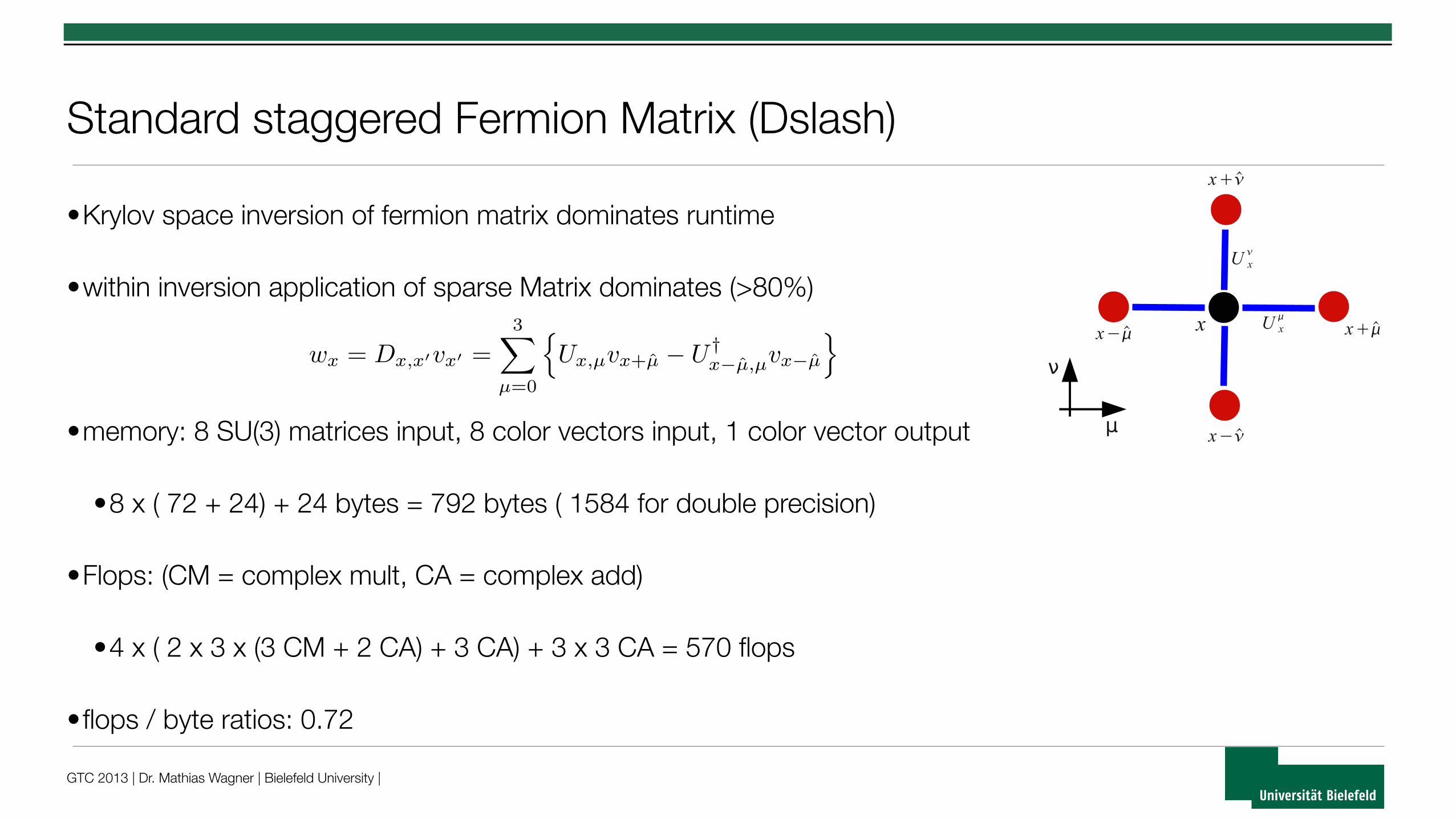
Standard staggered Fermion Matrix (Dslash)

•Krylov space inversion of fermion matrix dominates runtime

•within inversion application of sparse Matrix dominates (>80%)

wx

= Dx,x

0vx

0 =3

X

µ=0

n

Ux,µ

vx+µ

U †xµ,µ

vxµ

o















Mx = b. (1)


Mx,x0 = 12

4

µ=1

Pµ Uµ


+ (4 + m + Ax)x,x0

12Dx,x0 + (4 + m + Ax)x,x0 . (2)










Dx,x

0 = A =





•memory: 8 SU(3) matrices input, 8 color vectors input, 1 color vector output

•8 x ( 72 + 24) + 24 bytes = 792 bytes ( 1584 for double precision)

wx

= Dx,x

0vx

0 =3

X

µ=0

n

Ux,µ

vx+µ

U †xµ,µ

vxµ

o















Mx = b. (1)


Mx,x0 = 12

4

µ=1

Pµ Uµ


+ (4 + m + Ax)x,x0

12Dx,x0 + (4 + m + Ax)x,x0 . (2)










Dx,x

0 = A =





•memory: 8 SU(3) matrices input, 8 color vectors input, 1 color vector output

•8 x ( 72 + 24) + 24 bytes = 792 bytes ( 1584 for double precision)

•Flops: (CM = complex mult, CA = complex add)

•4 x ( 2 x 3 x (3 CM + 2 CA) + 3 CA) + 3 x 3 CA = 570 flops

•flops / byte ratios: 0.72

wx

= Dx,x

0vx

0 =3

X

µ=0

n

Ux,µ

vx+µ

U †xµ,µ

vxµ

o


Bandwidth bound

•memory bandwidth is crucial

•GTX cards are always faster

•even for double precision calculations

•linear algebra has an even worse flop / byte ratio

•vector addition c = a + b

• 48 bytes in, 24 bytes out, 6 flops →0.08 flops/byte

•flops are free - but registers are limited

•Dslash efficiency Tesla M2075: 0.72 flop/byte * 144 Gbytes/s = 103 Gflops (10% peak)


Bandwidth bound

•memory bandwidth is crucial

•GTX cards are always faster

•even for double precision calculations

•linear algebra has an even worse flop / byte ratio

•vector addition c = a + b

• 48 bytes in, 24 bytes out, 6 flops →0.08 flops/byte

•flops are free - but registers are limited

•Dslash efficiency Tesla M2075: 0.72 flop/byte * 144 Gbytes/s = 103 Gflops (10% peak)

Card GFlops (32 bit) GFlops (32 bit) GBytes/s Flops / byte Flops/ byte

GTX 580 1581 198 192 8.2 1.03

Tesla M2075 1030 515 144 7.2 3.6


Optimizing memory access

•use coalesced memory layout: structure of arrays (SoA) instead of AoS

•one can reconstruct a SU(3) matrix also from 8 or 12 floats

•improved actions result in matrices that are no longer SU(3):must load 18 floats






•exploit texture access: near 100% bandwidth

•ECC hurts (naive 12.5%, real world ~ 20-30 %)

•do more work with less bytes:→ mixed precision inverters (QUDA libray, Clark et al, CPC.181:1517,2010)

→ multiple right hand sides






•exploit texture access: near 100% bandwidth

•ECC hurts (naive 12.5%, real world ~ 20-30 %)

•do more work with less bytes:→ mixed precision inverters (QUDA libray, Clark et al, CPC.181:1517,2010)

→ multiple right hand sides

GTX580 (3GB)M2075 (6GB)

20

40

60

80

100

120

140

163.4 243.6 323.8 403.10 483.12 563.14 643.16 723.18

lattice size

Gflo

p/s

single precision

double precision

HISQ inverter on single GPU


Solvers for multiple right hand sides

•consider single precision for improved (HISQ) action

•need inversions for many (1500) ‘source’-vectors for a fixed gauge field (matrix)

•Bytes for n vectors

•Flops for n vectors

16 · (72 + n · 24) bytes + n · 24 bytes = 1152 bytes + 408 bytes · n .

1146 flops · n# r.h.s. 1 2 3 4 5flops/byte 0.73 1.16 1.45 1.65 1.8














Mx = b. (1)


Mx,x0 = 12

4

µ=1

Pµ Uµ


+ (4 + m + Ax)x,x0

12Dx,x0 + (4 + m + Ax)x,x0 . (2)










Dx,x

0 = A =















Mx = b. (1)


Mx,x0 = 12

4

µ=1

Pµ Uµ


+ (4 + m + Ax)x,x0

12Dx,x0 + (4 + m + Ax)x,x0 . (2)










Dx,x

0 = A =


+


Solvers for multiple right hand sides

•consider single precision for improved (HISQ) action

•need inversions for many (1500) ‘source’-vectors for a fixed gauge field (matrix)

•Bytes for n vectors

•Flops for n vectors

•Issue: register usage and spilling

•spilling for more than 3 r.h.s. with Fermi architecture

•already for more than 1 r.h.s. in double precision

16 · (72 + n · 24) bytes + n · 24 bytes = 1152 bytes + 408 bytes · n .

1146 flops · n

# registers stack frame spill stores spill loads SM 3.5 reg

12345

38 0 0 0 4058 0 0 0 6063 0 0 0 6563 40 76 88 7263 72 212 216 77

# r.h.s. 1 2 3 4 5flops/byte 0.73 1.16 1.45 1.65 1.8














Mx = b. (1)


Mx,x0 = 12

4

µ=1

Pµ Uµ


+ (4 + m + Ax)x,x0

12Dx,x0 + (4 + m + Ax)x,x0 . (2)










Dx,x

0 = A =















Mx = b. (1)


Mx,x0 = 12

4

µ=1

Pµ Uµ


+ (4 + m + Ax)x,x0

12Dx,x0 + (4 + m + Ax)x,x0 . (2)










Dx,x

0 = A =


+


Dslash-performance

•estimate performance from flop/byte ratio and available memory bandwidth

•full inversion should be roughly 10-15% lower

1 2 3 4 50

150

300

450

600M2075 est. GTX 580 est.K20 est. GTX Titan est.M2075 measured K20 measured

card M2075 GTX 580 K20 GTX Titan

Bandwidth [GB/s] 150 192 208 288

single precision


Dslash-performance



1 2 3 4 50

150

300

450


# registers stack frame spill stores spill loads SM 3.5 reg

12345

38 0 0 0 4058 0 0 0 6063 0 0 0 6563 40 76 88 7263 72 212 216 77


Bandwidth [GB/s] 150 192 208 288

single precision


Dslash-performance



1 2 3 4 50

150

300

450


1 2 3 4 50

75

150

225



Bandwidth [GB/s] 150 192 208 288

single precision

double precision


Linear algebra becomes relevant

•matrix operation (Dslash) for multiple r.h.s.

•linear algebra operations cannot

•float * vector + vector

•norms

•linear algebra scales linear #r.h.s.

Initialization

loop

Fermion Matrix

↵ =X

i

|~pA~p|i

~r = ~r !~p

~x = ~x+ !~p

i = |ri|

=X

i

i

~p = ~r + ~p






•norms


0

1500

3000

4500

6000

1 2 3

TIm

e [m

s]

Dslash Linear AlgebraInitialization

loop

Fermion Matrix

↵ =X

i

|~pA~p|i

~r = ~r !~p

~x = ~x+ !~p

i = |ri|

=X

i

i

~p = ~r + ~p






•norms


•for three r.h.s up to 25% of the runtime

0

1500

3000

4500

6000

1 2 3

TIm

e [m

s]

Dslash Linear Algebra

0

0,075

0,150

0,225

0,300

1 2 3

fraction LA

Initialization

loop

Fermion Matrix

↵ =X

i

|~pA~p|i

~r = ~r !~p

~x = ~x+ !~p

i = |ri|

=X

i

i

~p = ~r + ~p






•norms


•for three r.h.s up to 25% of the runtime

•more crucial for ‘cheaper’ matrix operations

0

1500

3000

4500

6000

1 2 3

TIm

e [m

s]


0

0,075

0,150

0,225

0,300

1 2 3

fraction LA

Initialization

loop

Fermion Matrix

↵ =X

i

|~pA~p|i

~r = ~r !~p

~x = ~x+ !~p

i = |ri|

=X

i

i

~p = ~r + ~p


Linear algebra: reducing PCI latencies

•Kernel calculates for each component i of each r.h.s. x:

•need to do reduction (→ see CUDA samples, M. Harris) for each r.h.s.

•copy data to host (one device to host copy for each r.h.s)

↵(x)i

= |r(x)i

|

↵0(x)j

=X

some i

↵(x)

i

0

1500

3000

4500

6000

1 2 3

TIm

e [m

s]


0

0,075

0,150

0,225

0,300

1 2 3

fraction LA


↵0 =↵0(x=0)j

, . . . ,↵0(x=N)j





•combine device to host copies to one for all r.h.s.

•last reduction step can be done on CPU or GPU

0

1500

3000

4500

6000

1 2 3 PCI latency

Tim

e [m

s]


0

0,075

0,150

0,225

0,300

1 2 3 PCI latency

fraction LA

↵(x)i

= |r(x)i

|

↵0(x)j

=X

some i

↵(x)

i


↵0 =↵0(x=0)j

, . . . ,↵0(x=N)j





•combine device to host copies to one for all r.h.s.

•last reduction step can be done on CPU or GPU

1 2 3 PCI latency0

1500

3000

4500

6000

Tim

e [m

s]


1 2 3 PCI latency0

0,075

0,150

0,225

0,300

fraction LA

↵(x)i

= |r(x)i

|

↵0(x)j

=X

some i

↵(x)

i





•copy data to host (one device to host copy for each r.h.s)0

1500

3000

4500

6000

1 2 3 PCI latency

Tim

e [m

s]


0

0,075

0,150

0,225

0,300

1 2 3 PCI latency

fraction LA

↵(x)i

= |r(x)i

|

↵0(x)j

=X

some i

↵(x)

i


Linear algebra: improve reduction

•standard way of doing reduction

•calculate floating point numbers that shall be reduced + reduction

•but data are already created on GPU0

1500

3000

4500

6000

1 2 3 PCI latency

Tim

e [m

s]


0

0,075

0,150

0,225

0,300

1 2 3 PCI latency

fraction LA





•but data are already created on GPU

•pre-reduction during ‘creation’

•does not affect runtime

•faster reduction (4x)

•tune parameter rc(enough threads)

0

1500

3000

4500

6000

1 2 3 PCI latency

Tim

e [m

s]


0

0,075

0,150

0,225

0,300

1 2 3 PCI latency

fraction LA





•but data are already created on GPU

•pre-reduction during ‘creation’

•does not affect runtime

•faster reduction (4x)

•tune parameter rc(enough threads)

0

1500

3000

4500

6000

1 3 pre-reduction


0

0,075

0,150

0,225

0,300

1 3 pre-reduction


Configuration generation on GPUs

•we use a full hybrid-monte Carlo simulation on GPU (HISQ action)

•no PCI bus bottleneck

•current runs with lattice size 323 x 8 in single precision

•ECC reduces memory bandwidth: costs roughly 30% performance

•lattices up to 483 x 12 fit on one Tesla cards with 6GB (double precision)

•runtime is an issue - at least use several GPUs in one node

•larger lattices (643 x 16) → use compute time on capacity computing machines (BlueGene)

•we aim at getting the best scientific output out of limited resources (#GPUs, available supercomputer time)


Registers pressure

•improved fermion action use smeared links

•require sum over products of up to 7 SU(3) matrices

•SU(3) Matrix: 18 / 36 registers






=∂

∂Ux,µ

⟨

Φ∣

∣

∣

[

M†[U ]M[U ]]−nf /4

∣

∣

∣Φ⟩

. (2.3)


[M†M]−nf /4 ≈ α0+∑l

αlM†M+βl

, (2.4)


∂Sf∂Ux,µ

= −∑lαl

⟨


∣

∣

∣

∂∂Ux,µ

(

M†[U ]M[U ])

∣

∣

∣

∣

[M†M+βl]−1Φ

⟩

= −∑lαl

(⟨

Xl∣

∣

∣

∣

∂D†[U ]

∂Ux,µ

∣

∣

∣

∣

Y l⟩

+

⟨

Y l∣

∣

∣

∣

∂D[U ]

∂Ux,µ

∣

∣

∣

∣

Xl⟩)

, (2.5)


[

fx,µ]

ab =∂Sf

∂[

Ux,µ]

ab=∑

y,ν(−1)yηy,ν

(

∂ [Uef fy,ν ]mn

∂ [Ux,µ ]ab

[

f (0)y,ν

]

mn+∂ [Uef f†


[

f (0)†y,ν

]

mn

)

, (2.6)


[

f (0)y,ν

]

mn=


l∗y ]m for even y

∑lαl[Xl


, (2.7)

3

Fermion force in MD→ take derivatives of smeared links with respect to ‘original’ links


Registers pressure

•improved fermion action use smeared links

•require sum over products of up to 7 SU(3) matrices

•SU(3) Matrix: 18 / 36 registers

•Fermi architecture: 63 registers / thread

•optimize SU(3) *= SU(3) operation for register usage

•spilling causes significant performance drop for bandwidth bound kernels

•however: spilling is often better than shared memory → 48kB L1 cache

•precomputed products help but must be stored somewhere






=∂

∂Ux,µ

⟨

Φ∣

∣

∣

[

M†[U ]M[U ]]−nf /4

∣

∣

∣Φ⟩

. (2.3)


[M†M]−nf /4 ≈ α0+∑l

αlM†M+βl

, (2.4)


∂Sf∂Ux,µ

= −∑lαl

⟨


∣

∣

∣

∂∂Ux,µ

(

M†[U ]M[U ])

∣

∣

∣

∣

[M†M+βl]−1Φ

⟩

= −∑lαl

(⟨

Xl∣

∣

∣

∣

∂D†[U ]

∂Ux,µ

∣

∣

∣

∣

Y l⟩

+

⟨

Y l∣

∣

∣

∣

∂D[U ]

∂Ux,µ

∣

∣

∣

∣

Xl⟩)

, (2.5)


[

fx,µ]

ab =∂Sf

∂[

Ux,µ]

ab=∑

y,ν(−1)yηy,ν

(

∂ [Uef fy,ν ]mn

∂ [Ux,µ ]ab

[

f (0)y,ν

]

mn+∂ [Uef f†


[

f (0)†y,ν

]

mn

)

, (2.6)


[

f (0)y,ν

]

mn=


l∗y ]m for even y

∑lαl[Xl


, (2.7)

3

Fermion force in MD→ take derivatives of smeared links with respect to ‘original’ links


Optimizing register usage / reduce spilling

•e.g. force for the 7 link term consists of 56 products of 7 SU(3) matrices ( x 24 for ‘rotations’ )

•limited GPU memory: store precomputed products ?

v201203: initial version

v201204: optimized matrix mult, split into servel Kernels

v201207: minor changes for memory access

v201211: reorganized split up Kernel

v201303: reconstruction of matrices from 14 floats









v201303: reconstruction of matrices from 14 floats v201203 v201204 v201207 v201211 v2013030

7500

15000

22500

30000

Tim

e [m

s] M2075 single K20 singleM2075 double K20 double










7500

15000

22500

30000

Tim

e [m


v201203 v201204 v201207 v201211 v2013030

1,00

2,00

3,00

4,00

single M2075/K20double M2075/K20










7500

15000

22500

30000

Tim

e [m


v201203 v201204 v201207 v201211 v2013030

1,00

2,00

3,00

4,00

single M2075/K20double M2075/K20

0

1,00

2,00

3,00

4,00

v201203 v201207 v201303

M2075 double/singleK20 double/single


Status of lattice data

0

0.1

0.2

0.3 r2B

Tc=154(9)MeV

No=68

0

0.05

0.1r4

B BNL-Bielefeldpreliminary

-0.5

0

0.5

140 160 180 200 220 240

r6B

T [MeV]

0

0.2

0.4

0.6 r2Q

Tc=154(9)MeV

No=68

0

0.1

0.2

0.3 r4Q BNL-Bielefeld

preliminary

-1-0.5

0 0.5

1

140 160 180 200 220 240

r6Q

T [MeV]

0

0.2

0.4

0.6

0.8 r2S

Tc=154(9)MeV

No=68

0

0.2

0.4

0.6 r4S

BNL-Bielefeldpreliminary

-1-0.5

0 0.5

1 1.5

140 160 180 200 220 240

r6S

T [MeV]

•highly-improved staggered quarks, close to physical pion mass ( )ml/ms = 1/20


Freeze-out curve from heavy-ion collision

0

0.16

FAIR@GSI

hadron gas

quark-gluon-plasma


vacuum

RHIC@BNL

chemical potentialµB

T [

GeV

]

NICA@JINR

initial conditions




0

0.16

FAIR@GSI

hadron gas

quark-gluon-plasma


vacuum

RHIC@BNL


T [

GeV

]

NICA@JINR

initial conditions


evolution



0

0.16

FAIR@GSI

hadron gas

quark-gluon-plasma


vacuum

RHIC@BNL


T [

GeV

]

NICA@JINR

initial conditions


Lattice EoS

evolution



0

0.16

FAIR@GSI

hadron gas

quark-gluon-plasma


vacuum

RHIC@BNL


T [

GeV

]

NICA@JINR

initial conditions


freeze-out

Lattice EoS

freeze-outevolution



0

0.16

FAIR@GSI

hadron gas

quark-gluon-plasma


vacuum

RHIC@BNL


T [

GeV

]

NICA@JINR

initial conditions


140

145

150

155

160

165

170

175

180

185

10 20 30 40 50 60

µb (MeV)

T (M

eV)

T=165.5, µb=38 MeV, χ2=4.1/11

√sNN=130 GeV

10-3

10-2

10-1

1

Rat

io

√sNN=130 GeV

Data

ModelT=165.5, µb=38 MeV

π-

π+K-

K+p–

pΛ–

Λ

Ξ–

Ξ

Ω–

Ω

K+

π+K-

π-p–

π-Λ–

π-Ξ

π-Ω

π-φ

K-K*

K-

Fig. 10. The χ2 distribution and hadron yield ratios with best fit at√

sNN=130 GeV. Here, theΩ yield includes both Ω and Ω.

MeV, µb = 38 ± 11 MeV, χ2/Ndf=4.1/11.

Although the fit is good for all cases (and even if the minimal χ2 is obtained for case i), weconsider the intermediate case iii) as the most likely situation, as it could be an implicitresult of the reconstruction in the experiment. The outcome of the fit is shown in Fig. 10.The very good fit is also apparent in the comparison of the hadron ratios: essentially allthe experimental ratios are well reproduced by the model, including those involving φ andK∗ resonances.

At√

sNN=200 GeV only a limited set of yields of identified hadrons is available to date.The yields of π±, K±, p, and p are published by PHENIX [76], STAR [77], and BRAHMS[78] and the values agree within the quoted systematic errors. In addition, available arethe yields of φ [79,80], K(892)∗ [81], d and d [82]. We use the hadron ratios with thecorresponding errors whenever provided by the experiments [76,79,80,81] or otherwisecalculate the ratios using the published yields quoted above. Further ratios are availableas preliminary data on strange hyperon ratios [83], ∆++/p [84], p/π−, Λ/π−, Ξ/π−, Ω/π−,and Λ∗/Λ[85]. Unless specified, our fits do not include the ratios involving resonances(∆++/p, K(892)∗, and Λ∗).

We consider the following cases for the fits:i) a combined fit of all available data, with the exception of strongly decaying resonances:T = 155 ± 2 MeV, µb = 26 ± 5 MeV, χ2/Ndf = 34.1/23 (with δ2 minimization: T=164MeV, µb=24 MeV, δ2=0.40). If we include in the fit the three ratios involving resonances(K∗/K−, Λ∗/Λ, and ∆++/p), the results are the same within the errors, T = 155 ± 2MeV, µb = 25 ± 5 MeV, but with a worse χ2/Ndf = 41.8/26 (T=162 MeV, µb=22 MeV,δ2=0.82).ii) as i), but excluding from the fit the ratios p/π− and φ/K− from PHENIX. The result-ing parameters are: T = 160.5± 2 MeV, µb = 20± 4 MeV, with χ2/Ndf=16.0/21 (T=166MeV, µb=26 MeV, δ2=0.19). Including the resonances the outcome of the fit is identical,T = 160 ± 2 MeV, µb = 20 ± 4 MeV, with a reasonable χ2/Ndf = 25.2/24 (T=164 MeV,

Hadron abundancesfrom HRG model

freeze-out

Lattice EoS

freeze-outevolution



0

0.16

FAIR@GSI

hadron gas

quark-gluon-plasma


vacuum

RHIC@BNL


T [

GeV

]

NICA@JINR

initial conditions


140

145

150

155

160

165

170

175

180

185

10 20 30 40 50 60

µb (MeV)

T (M

eV)

T=165.5, µb=38 MeV, χ2=4.1/11

√sNN=130 GeV

10-3

10-2

10-1

1

Rat

io

√sNN=130 GeV

Data

ModelT=165.5, µb=38 MeV

π-

π+K-

K+p–

pΛ–

Λ

Ξ–

Ξ

Ω–

Ω

K+

π+K-

π-p–

π-Λ–

π-Ξ

π-Ω

π-φ

K-K*

K-

Fig. 10. The χ2 distribution and hadron yield ratios with best fit at√

sNN=130 GeV. Here, theΩ yield includes both Ω and Ω.

MeV, µb = 38 ± 11 MeV, χ2/Ndf=4.1/11.

Although the fit is good for all cases (and even if the minimal χ2 is obtained for case i), weconsider the intermediate case iii) as the most likely situation, as it could be an implicitresult of the reconstruction in the experiment. The outcome of the fit is shown in Fig. 10.The very good fit is also apparent in the comparison of the hadron ratios: essentially allthe experimental ratios are well reproduced by the model, including those involving φ andK∗ resonances.

At√

sNN=200 GeV only a limited set of yields of identified hadrons is available to date.The yields of π±, K±, p, and p are published by PHENIX [76], STAR [77], and BRAHMS[78] and the values agree within the quoted systematic errors. In addition, available arethe yields of φ [79,80], K(892)∗ [81], d and d [82]. We use the hadron ratios with thecorresponding errors whenever provided by the experiments [76,79,80,81] or otherwisecalculate the ratios using the published yields quoted above. Further ratios are availableas preliminary data on strange hyperon ratios [83], ∆++/p [84], p/π−, Λ/π−, Ξ/π−, Ω/π−,and Λ∗/Λ[85]. Unless specified, our fits do not include the ratios involving resonances(∆++/p, K(892)∗, and Λ∗).

We consider the following cases for the fits:i) a combined fit of all available data, with the exception of strongly decaying resonances:T = 155 ± 2 MeV, µb = 26 ± 5 MeV, χ2/Ndf = 34.1/23 (with δ2 minimization: T=164MeV, µb=24 MeV, δ2=0.40). If we include in the fit the three ratios involving resonances(K∗/K−, Λ∗/Λ, and ∆++/p), the results are the same within the errors, T = 155 ± 2MeV, µb = 25 ± 5 MeV, but with a worse χ2/Ndf = 41.8/26 (T=162 MeV, µb=22 MeV,δ2=0.82).ii) as i), but excluding from the fit the ratios p/π− and φ/K− from PHENIX. The result-ing parameters are: T = 160.5± 2 MeV, µb = 20± 4 MeV, with χ2/Ndf=16.0/21 (T=166MeV, µb=26 MeV, δ2=0.19). Including the resonances the outcome of the fit is identical,T = 160 ± 2 MeV, µb = 20 ± 4 MeV, with a reasonable χ2/Ndf = 25.2/24 (T=164 MeV,

Hadron abundancesfrom HRG model

freeze-out

Tf(ps), µf(

ps), Vf(

ps)

Lattice EoS

freeze-outevolution



0

0.16

FAIR@GSI

hadron gas

quark-gluon-plasma


vacuum

RHIC@BNL


T [

GeV

]

NICA@JINR

initial conditions


freeze-out

Tf(ps), µf(

ps), Vf(

ps)

Lattice EoS

freeze-outevolution

11

structure consistent with O(4) critical behavior at µB = 0, m = 0

2) Status of the lattice data

Christian SchmidtBielefeld

r4B BNL-Bielefeld

preliminary

0

0.05

0.1

r4B BNL-Bielefeld

preliminary

0

0.05

0.1

r2B

No=6

0

0.1

0.2

0.3

Tc=154(9) MeV

r2B

No=68

0

0.1

0.2

0.3

Tc=154(9) MeV

r6B

-1.5-1

-0.5 0

0.5 1

1.5

120 140 160 180 200 220 240T [MeV]

r4Q


0.15 0.2

0.25 0.3

0.35

r4Q


0.15 0.2

0.25 0.3

0.35

r2Q

No=6

0 0.1 0.2 0.3 0.4 0.5 0.6 0.7

Tc=154(9) MeV

r2Q

No=68

0 0.1 0.2 0.3 0.4 0.5 0.6 0.7

Tc=154(9) MeV

r6Q

-1.5-1

-0.5 0

0.5 1

1.5

120 140 160 180 200 220 240T [MeV]

r6Q

-1.5-1

-0.5 0

0.5 1

1.5

120 140 160 180 200 220 240T [MeV]

r6Q

-1.5-1

-0.5 0

0.5 1

1.5

120 140 160 180 200 220 240T [MeV]

Donnerstag, 16. August 12

Fluctuations from Lattice QCD


Pinning down the freeze-out parameters

•need two experimental ratios to determine

•baryon number fluctuations are not directly accessible in experiments

•we consider ratios of electric charge fluctuations

MQ(ps)

2Q(

ps)

=hNQi

h(NQ)2i=

Q1 (T, µB)

Q2 (T, µB)

= RQ,112 µB + RQ,3

12 µ3B + · · · = RQ

12(T, µB)

SQ(ps)3

Q(ps)

MQ(ps)

=

(NQ)3

↵

hNQi=

Q3 (T, µB)

Q1 (T, µB)

= RQ,031 + RQ,2

31 µ2B + · · · = RQ

31(T, µB)

LO linear in , fixesµB µfB

LO independent of , fixesµB T f

S

M

: mean: variance: skewness

(T f , µfB)


Determination of freeze-out temperature

•small cutoff effects

•small NLO corrections (<10%) for μ/T < 1.3

µB/T=1µB/T=0No=6No=8

0.0

0.5

1.0

1.5

2.0

2.5

3.0

140 150 160 170 180 190 200 210 220 230 240

T [MeV]

R31Q

HRG

free

RQ31(T, µB) = RQ,0

31 + RQ,231 µ2

B

Bands: Continuum estimate

BNL-BI, PRL 109 (2012) 192302


Determination of freeze-out temperature

•small cutoff effects


µB/T=1µB/T=0No=6No=8

0.0

0.5

1.0

1.5

2.0

2.5

3.0

140 150 160 170 180 190 200 210 220 230 240

T [MeV]

R31Q

HRG

free

RQ31(T, µB) = RQ,0

31 + RQ,231 µ2

B

T f [MeV ]SQ3Q/MQ

& 2

1.5

. 1

. 155

160

& 165

Bands: Continuum estimate

BNL-BI, PRL 109 (2012) 192302


Determination of freeze-out chemical potential

•small cutoff effects at NLO


Bands: LO Continuum extrapolation NLO Continuum estimate

RQ12(T, µB) = RQ,1

12 µB + RQ,312 µ3

B

BNL-BI, PRL 109 (2012) 192302

LONo=6No=8No=12

0.05

0.07

0.09

0.11

0.13R12

Q,1

HRG

free

NLO

-0.04

0.00

0.04

0.08

0.12

140 150 160 170 180 190 200 210 220 230 240

T [MeV]

R12Q,3/R12

Q,1

HRG

free


Determination of freeze-out chemical potential

•small cutoff effects at NLO


Bands: LO Continuum extrapolation NLO Continuum estimate

RQ12(T, µB) = RQ,1

12 µB + RQ,312 µ3

B

µfB/T fMQ/2

Q

0.01-0.02 0.1-0.2

0.03-0.04 0.3-0.40.05-0.08 0.5-0.7

T f 160 MeV(for )

BNL-BI, PRL 109 (2012) 192302

0.000.010.020.030.040.050.060.070.080.090.100.110.120.130.140.15

0.0 0.1 0.2 0.3 0.4 0.5 0.6 0.7 0.8 0.9 1.0 1.1 1.2 1.3

µB/T

R12Q

HRG

T = 150 MeV

T = 160 MeV

T = 170 M

eV

LONo=6No=8No=12

0.05

0.07

0.09

0.11

0.13R12

Q,1

HRG

free

NLO

-0.04

0.00

0.04

0.08

0.12

140 150 160 170 180 190 200 210 220 230 240

T [MeV]

R12Q,3/R12

Q,1

HRG

free


Summary

•GPUs enable breakthroughs in Lattice QCD

•Experiences with Lattice QCD on the Bielefeld GPU cluster

•Tuning single GPU performance for staggered fermion

•Lattice QCD is bandwidth bound


Summary

•GPUs enable breakthroughs in Lattice QCD

•Experiences with Lattice QCD on the Bielefeld GPU cluster

•Tuning single GPU performance for staggered fermion

•Lattice QCD is bandwidth bound

•multi-GPU for larger systems

•Kepler provides a major speedup for double precision (thanks to registers)

•GTX Titan should allow for > 500 GFlops in single precision (>250 GFlops double)

•running production on CPUs and do ‘live-measurements’ on the GPU for Titan


Accelerating Lattice QCD simulations with brain power• Bielefeld Group

Edwin LaermannFrithjof KarschOlaf KaczmarekMarkus KlappenbachMathias WagnerChristian SchmidtDominik SmithHiroshi OnoSayantan SharmaMarcel MüllerThomas LutheLukas Wresch

• Brookhaven GroupPeter PetreczkySwagato MukherjeeAlexei BazavovHeng-Tong DingPrasad HegdeYu Maezawa

• collaboratorsWolfgang Söldner (Regensburg)Piotr Bialas (Krakow)

• supportersMike Clark (Nvidia)

Matthias Bach (FIAS)

Contact: [email protected]

mailto:[email protected]

mailto:[email protected]

GPUs Immediately Relating Lattice QCD to Collider Experiments

Documents

Transcript of GPUs Immediately Relating Lattice QCD to Collider Experiments