Department of Construction Sciences

Solid Mechanics

ISRN LUTFD2/TFHF–10/5160-SE(1-34)

GPU parallelization of

crystal plasticity FE analyses

Master Thesis by

Per Johansson

SUPERVISOR

HÅKAN HALLBERG AND YLVA MELLBIN, DIV. OF SOLID MECHANICS

EXAMINER

PROF. MATTI RISTINMAA, DIV. OF SOLID MECHANICS

Copyright c© 2011 by Div. of Solid Mechanics and Per Johansson

Printed by Media-Tryck, Lund ,Sweden

For information, address:

Division of Solid Mechanics, Lund University, Box 118, SE-221 00 Lund, Sweden.

Homepage: http://www.solid.lth.se

Preface

This master thesis has been carried out at Lund Institute of Technology atthe division of Solid Mechanics as the last part of my Master in MechanicalEngineering.

I would like to address thanks to my two supervisors Håkan Hallberg and YlvaMellbin for their support during this work.

Malmö, March 2011

Per Johansson

II

Abstract

Polycrystalline materials are defined as materials that contain several grainsoriented in different directions. The material model used for polycrystallinematerials can for example be crystal plasticity where each grain, on a micro-scopic level is observed in the aspects of stresses and stiffness.

What many do not realize is that a computer’s graphics card also include aprocessing hardware, GPU (Graphics Processing Unit) that have previously onlybeen used in calculations related to computer graphics. This type of hardwareconsist of a multi-core processing unit to do massively parallel calculations. Thistechnology can have a big impact on the computationally demanding analysisas crystal plasticity.

In this thesis a FE analysis, where the material behavior is described by a crystalplasticity model, has been changed to be executed on the GPU, this resulted ina speed up dependant of the number of grains considered. The result have onlyspeed up impact when the number of grains are over 400, around 1200 the totalspeed up are around 2 times the original CPU program. Although the resultsshow a positive increase in speed, this is not a programming structure that issuitable for GPU calculation, due to many constraints of syntax and a memorymanagement that is not suitable for the GPU.

IV

Contents

1 Introduction 11.1 Objectives . . . . . . . . . . . . . . . . . . . . . . . . . . . . . . . 11.2 Disposition . . . . . . . . . . . . . . . . . . . . . . . . . . . . . . 1

2 Background - CUDA and GPU programming 22.1 CUDA . . . . . . . . . . . . . . . . . . . . . . . . . . . . . . . . . 2

2.1.1 CUDA Overview . . . . . . . . . . . . . . . . . . . . . . . 32.1.2 CUDA Memory Overview . . . . . . . . . . . . . . . . . . 42.1.3 Specification TESLA C2050 . . . . . . . . . . . . . . . . . 5

2.2 PGI CUDA Fortran . . . . . . . . . . . . . . . . . . . . . . . . . 62.2.1 SUBROUTINE and FUNCTIONS . . . . . . . . . . . . . 72.2.2 Variable attributes . . . . . . . . . . . . . . . . . . . . . . 82.2.3 Compute compatibility . . . . . . . . . . . . . . . . . . . . 92.2.4 Examples . . . . . . . . . . . . . . . . . . . . . . . . . . . 10

2.3 CULA . . . . . . . . . . . . . . . . . . . . . . . . . . . . . . . . . 14

3 Background - Crystal plasticity 153.1 Polycrystalline materials . . . . . . . . . . . . . . . . . . . . . . . 15

3.1.1 Crystal plasticity model . . . . . . . . . . . . . . . . . . . 163.1.2 Numeric implementation . . . . . . . . . . . . . . . . . . . 19

4 Implementation 214.1 CUDA implementation of crystal plasticity . . . . . . . . . . . . 21

5 Results and Conclusion 235.1 Speed increase . . . . . . . . . . . . . . . . . . . . . . . . . . . . 235.2 Conclusion . . . . . . . . . . . . . . . . . . . . . . . . . . . . . . 25

5.2.1 Recommendation . . . . . . . . . . . . . . . . . . . . . . . 25

VI

Chapter 1

Introduction

In the material model crystal plasticity for polycrystalline materials each grain,on a microscopic level is observed in the aspects of stresses and stiffness. Inrecent years the development of graphics cards has made it possible to use a newprogramming technology that uses the graphics card’s multi- core processingunit to do massively parallel calculations. This technology can have a big impacton the computationally demanding analysis of polycrystalline materials.

GPU programming is evaluated by implementing crystal plasticity FE analysison a Cook’s membrane where grain stiffness and tension are calculated on thegraphic card. The influence the number of grain has on the calculation speed isalso examined by changing the number of grains in the analysis.

1.1 Objectives

The purpose of this thesis is to study the use of parallel programming whensolving FE equations using polycrystalline materials. The programming ar-chitecture evaluated is CUDA in the language FORTRAN through PortlandGroups compiler CUDA FORTRAN.

1.2 Disposition

The report begins with a short background on CUDA and also on modelingof polycrystalline materials. The next chapter starts with the numerical im-plementation followed by the implementation and the changes due to the im-plementation of CUDA architecture. The last chapter consists of results andconclusions.

1

Chapter 2

Background - CUDA and

GPU programming

2.1 CUDA

Regular programs typically uses the computer’s CPU (Central Processing Unit)to solving calculation problems. What many do not realize is that a computer’sgraphics card also include a processing hardware, GPU (Graphics ProcessingUnit) that have previously only been used in calculations related to computergraphics. In recent years, a massive performance development has been takingplace on the graphics cards due to the demands of the gaming industry.

In 2007 the graphics card developer NVIDIA introduced a new technology calledCUDA (Compute Unified Device Architecture) that is an architecture that havemade it possible to handle calculations on both the CPU and the GPU using theprogramming language C. This have made it possible to use the big advantageof parallel calculation on the multi core GPU.

After NVIDIA’s launch several software companies processed the technology,such as the Portland Group, which has developed a FORTRAN compiler seesection 2.2. Also EM Photonics, which has developed a library correspondingto LAPACK performing linear algebra calculations in parallel on the GPU formore info see section 2.3.

2

2.1.1 CUDA Overview

Some of NVIDIAs CUDA architecture terminology is listed below and will beused throughout the thesis.

Host Application or data handled by the CPU.

Device Application or data handled by the GPU.

Kernel Application written to be executed on the GPU.

Thread An execution of a kernel with a given index.

Block A group of threads.

Grid A group of blocks. The grid is handled and executed on a single device(GPU chip)

MP The GPU chips are organized in a collection of multiprocessors (MP) whereone MP is responsible of handling one or more blocks in a grid. When thenumber of blocks are bigger than number of MPs a schedule will determinewhich block will be executed.

SP Each MP is divided into a number of stream processors (SP). Where eachSP is handling one or more threads in a block.

The total amount of CUDA cores are defined by MP x SP.

In this context a application can be a main-, sub- program or function.

3

2.1.2 CUDA Memory Overview

CUDA memory spaces differs from the usual host memory, first because it isa hardware card that comes with its own synchronous dynamic random accessmemory (SDRAM), corresponding to an ordinary RAM memory which everycomputer has. In order to execute a program on the GPU, this requires thatmemory transfers from the host memory to the memory allocated on the device.Then, to examine the results it is necessary to transfer it back to the host fromthe device.

• Device code can:– R/W per-thread registers

– R/W per-thread local memory

– R/W per-block shared memory

– R/W per-grid global memory

– Read only per-grid constant

memory

• Host code can

– R/W per grid global and

constant memories

(Device) Grid

ConstantMemory

GlobalMemory

Block (0, 0)

Shared Memory

Thread (0, 0)

Registers

Thread (1, 0)

Registers

Block (1, 0)

Shared Memory

Thread (0, 0)

Registers

Thread (1, 0)

Registers

Host

Figure 2.1: CUDA memory overview [2]

Global Memory

As seen in figure 2.1 the global memory is accessible during read or write fromthe host and also from the unique threads in the device. This is a big memorystored off chip in a bank of SDRAM chips, which makes it very slow to access.The reason for this is that the location on SDRAM tends to have long accesslatencies and also a finite access bandwidth. This can result in a poor executiontime with too many threads with global memory requests. This memory typecan also be called device memory.

Shared Memory

A small memory located on the chip, divided between the blocks. This memoryis only accessible for threads within the block that are executed by the currentMP. Due to the fact that it is stored on the chip contribute to high accessperformance.

4

Constant Memory

A read-only memory type for the device but read or write accessible for thehost. Constant memory is also located on the chip which makes the accessperformance very high.

Registers

A scalar memory type that is assigned to each thread. It is handled by, andlocated on, the MP which makes the access performance very good. Whenregisters runs out each thread gets assigned local memory which is located inthe global memory.

Local Memory

A read or write memory for each thread located on the global memory whichmakes it also very slow to access.

2.1.3 Specification TESLA C2050

The card used in this thesis is NVIDIA TESLA C2050, the specification is shownbelow.

CUDA Capability version: 2.0Number of cores: 14 (MP) x 32 (SP) = 448Clock rate: 1.15 GHzTotal amount of global memory: 2817982464 bytesTotal amount of constant memory: 65536 bytesTotal amount of shared memory per block: 49152 bytesTotal number of registers available per block: 32768Maximum size of each dimension of a block: 1024 x 1024 x 64Maximum size of each dimension of a grid: 65535 x 65535 x 1

5

2.2 PGI CUDA Fortran

The Portland Group Inc have developed a compiler called PGI CUDA Fortranwhich has a built-in support for using CUDA architecture in addition to stan-dard FORTRAN.

CUDA C and also CUDA Fortran are lower-level explicit programming modelstogether with a library of runtime components that gives the programmer adirect control of most aspects of GPU programming.

When NVIDIA launched CUDA the main area was computational parallel pro-gramming, this through various libraries and a C compiler, CUDA C. CUDAfortran as well as CUDA C is a lower-level explicit programming model withmany runtime library components.

CUDA Fortran makes it possible to use the following operations in a fortranprogram

-Declaring variables that are allocated in the GPU device memory

-Allocating dynamic memory in the GPU device memory

-Copying data from the host memory to the GPU memory , and back

-Writing subroutines and functions to execute on the GPU

-Invoking GPU subroutines from the host

CUDA Fortran is built by using the PGI Fortran compiler with the filenameextension .cuf which is a free-format CUDA Fortran. Although the flag -Mcuda

is required by the PGI Fortran compiler.

6

2.2.1 SUBROUTINE and FUNCTIONS

To designate where a subroutine or function will be executed is defined throughadditional attributes as:

Attributes(host)

This type of declaration is the same as in standard FORTRAN, and is also thedefault when no attribute is declared and will just mean that the subroutine isexecuted on the host.

Attributes(global)

A subroutine with the attribute global is a kernel subroutine or also called devicekernel, because it is executed on the device. Invoking of a device kernel is doneby the use of special chevron, which determines the number of thread blocksthat will be used and the number of threads containing in each thread block.

Parallelization is done according to the number of threads and blocks that arespecified when invoking the device kernel. The device kernel will then be ex-ecuted in parallel with the only difference that the internal variables threadidx

and blockidx will vary between 1 and the number of threads and blocks thatyou define at the call of the device kernel. By calling a device kernel with 1, 1within chevrons makes it a non parallel execution. This can be usefull if youwant to call a subroutine that will be execution on the GPU as serial code.

Example:

attributes(global) subroutine kernel(...)

...

To invoke a device kernel:

call kernel<<<dimGrid,dimBlock>>>(...)

Attributes(device)

A subroutine or function with the attribute device will be compiled for executionon the device. This type of subroutine or function can only be invoked byanother subroutine with the attribute device or global and must also appear inthe same MODULE as the subroutine that invoked it.

Example:

attributes(device) subroutine deviceSub(...)

...

attributes(device) function deviceFunc(...)

...

7

Restrictions on the device subprogram

A subroutine or function with the attribute global or device is a device sub-program and has to satisfy some restrictions. It can’t call a host subroutine orfunction, neither can it be recursive. There are also restriction in standard For-tran intrinsic functions, for example MATMUL is not allowed. Input and outputstatements as for example READ,WRITE and PRINT are not allowed either.Objects with the attribute pointer or allocatable are not allowed in subprogramsand neither are automatic arrays without fixed size. Device subprogram can’thandle a temporary array definition for example

A = (/1,1,1/)

which is the standard way to assign an array, instead it have to be done elementwise.

2.2.2 Variable attributes

Device data

The attribute device define the array to be in the global memory space. Thedeclaration of device data is made according to:

double precision, device :: a(10)

When calling a device subprograms with dummy arguments, to get the corre-sponding size a integer with the attribute value have to be declared. Integerwith the attribute value don’t have to be located on the device memory whichcan be usefull in other cases as well.

attributes(global) subroutine dev_kernel(a,b,n)

double precision, dimension(n,n) :: a,b

integer, value :: n

here are a and b dummy arrays and n dummy argument.

Shared data

The attribute shared defines the array to be located at the chip (in the sharedmemory) and must follow the same criterion as the device data type.

double precision, shared :: a(10)

Constant data

The attribute constant defines the array to be of the type constant data andcan be define according to

double precision, constant :: a(10)

As defined in section 2.1.2, constant data can only be written by the host.Constant data arrays have to be fixed size and can not be allocatable.

8

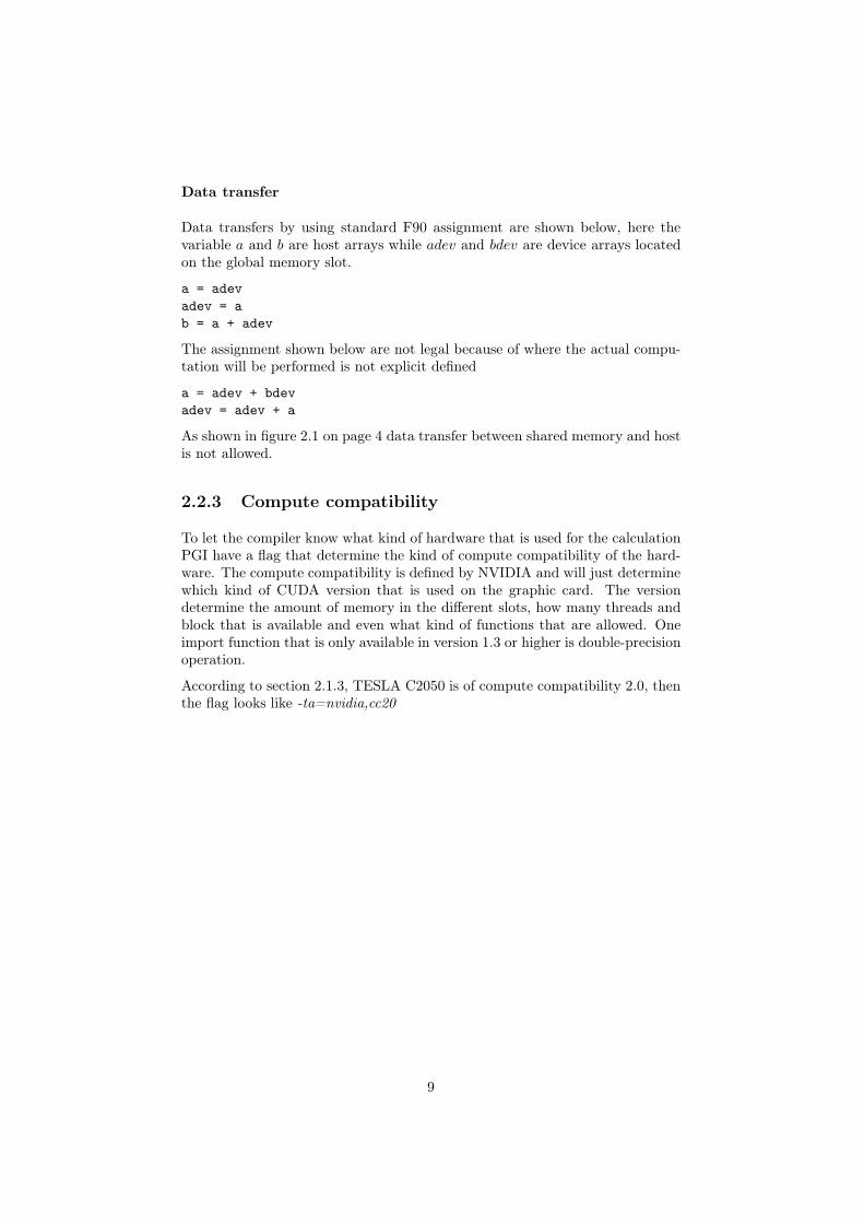
Data transfer

Data transfers by using standard F90 assignment are shown below, here thevariable a and b are host arrays while adev and bdev are device arrays locatedon the global memory slot.

a = adev

adev = a

b = a + adev

The assignment shown below are not legal because of where the actual compu-tation will be performed is not explicit defined

a = adev + bdev

adev = adev + a

As shown in figure 2.1 on page 4 data transfer between shared memory and hostis not allowed.

2.2.3 Compute compatibility

To let the compiler know what kind of hardware that is used for the calculationPGI have a flag that determine the kind of compute compatibility of the hard-ware. The compute compatibility is defined by NVIDIA and will just determinewhich kind of CUDA version that is used on the graphic card. The versiondetermine the amount of memory in the different slots, how many threads andblock that is available and even what kind of functions that are allowed. Oneimport function that is only available in version 1.3 or higher is double-precisionoperation.

According to section 2.1.3, TESLA C2050 is of compute compatibility 2.0, thenthe flag looks like -ta=nvidia,cc20

9

2.2.4 Examples

To describe the benefits of using GPU parallelization and the differences com-pared to serial CPU programs follows here an example of a matrix multiplicationthat is well suited to parallelize using CUDA.

This program parallelizes using sub matrix multiplication and to avoid globalmemory request, the sub matrices are copied to the shared memory. As de-scribed in section 2.2.3 the hardware that is used is of compute compatibility2.0 that makes it possible to use maximum sub matrix sizes of 32x32 otherwisethe shared memory block will be too small.

0 2000 4000 6000 8000 10000 120000

200

400

600

800

1000

1200Time to calculate Matrix multiplication

Number of rows and cols

Tim

e (s

)

GPU matmul

sun

intel −O3

pgfortran three nestled loop

Figure 2.2: Example comparing MATMUL

A possible reason for the unusual appearance of intel-O3 can be that the curveis created by ALLOCATE and DEALLOCATE a certain matrix size that canbe divided by 32 in a do loop, because this is the best way to use the GPU code.This may have contributed to the irregular appearance of the graphs in figure2.2.

10

0 2000 4000 6000 8000 10000 120000

2

4

6

8

10

12

14GPU times faster than SUN

Number of rows and cols

Tim

es fa

ster

Passes 1 at 100 rows/cols

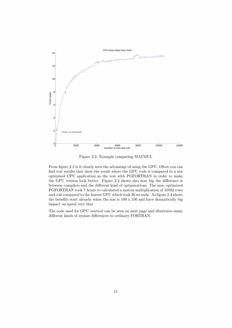
Figure 2.3: Example comparing MATMUL

From figure 2.2 is it clearly seen the advantage of using the GPU. Often you canfind test results that show the result where the GPU code is compared to a notoptimized CPU application as the test with PGFORTRAN in order to makethe GPU version look better. Figure 2.2 shows also how big the difference isbetween compilers and the different kind of optimizations. The non- optimizedPGFORTRAN took 7 hours to calculated a matrix multiplication of 10592 rowsand cols compared to the fastest GPU which took 26 seconds. As figure 2.3 showsthe benefits start already when the size is 100 x 100 and have dramatically bigimpact on speed over that.

The code used for GPU matmul can be seen on next page and illustrates manydifferent kinds of syntax differences to ordinary FORTRAN.

11

module mmul_mod

use cudafor

contains

!!! mmul_kernel computes A*B into C where A is NxM, B is MxL, C is then NxL

attributes(global) subroutine mmul_kernel( A, B, C, N, M, L )

double precision, device :: A(N,M), B(M,L), C(N,L)

integer, value :: N, M, L

integer :: i, j, kb, k, tx, ty

!!! submatrices are declared to be in CUDA shared memory

double precision, shared :: Asub(32,32), Bsub(32,32)

!!! the value of C(i,j) being computed, a temporary scalar

double precision :: Cij

!!! Start execution, first get my thread indices

tx = threadidx%x

ty = threadidx%y

!!! This thread computes C(i,j) = sum(A(i,:) * B(:,j))

i = (blockidx%x-1) * 32 + tx

j = (blockidx%y-1) * 32 + ty

Cij = 0D0

!!! Do the k loop in chunks of 32, the block size

do kb = 1, M, 32

!!! Fill the submatrices; each of 32x32 threads in the thread block loads

!!! one element of Asub and Bsub

Asub(tx,ty) = A(i,kb+ty-1)

Bsub(tx,ty) = B(kb+tx-1,j)

!!! Wait until all elements are filled

call syncthreads()

!!! Multiply the two submatrices; ! Each of the 32x32 threads accumulates the

!!! dot product for its element of C(i,j)

do k = 1,32

Cij = Cij + Asub(tx,k) * Bsub(k,ty)

enddo

!!! Synchronize to make sure all threads are done reading the submatrices before

!!! overwriting them in the next iteration of the kb loop

call syncthreads()

enddo

12

!!! Each of the 32x32 threads stores its element to the global C array

C(i,j) = Cij

end subroutine mmul_kernel

!!! The host routine to drive the matrix multiplication

subroutine mmul( A, B, C )

!!! assumed shape input arrays

double precision, dimension(:,:) :: A, B, C

!!! Array dimensions

integer :: N, M, L

!!! allocatable device arrays

double precision, device, allocatable, dimension(:,:) :: Adev,Bdev,Cdev

!!! dim3 variables to define the grid and block shapes, predefined in cudafor

type(dim3) :: dimGrid, dimBlock

integer :: r

!!! Begin execution, first determine the sizes of the input arrays

N = size( A, 1 )

M = size( A, 2 )

L = size( B, 2 )

!!! Allocate the device arrays using F90 ALLOCATE

allocate( Adev(N,M), Bdev(M,L), Cdev(N,L) )

!!! Copy A and B to the device using F90 array assignments

Adev = A(1:N,1:M)

Bdev = B(1:M,1:L)

!!! Create the grid and block dimensions

dimGrid = dim3( N/32, L/32, 1 )

dimBlock = dim3( 32, 32, 1 )

!!! Launch the GPU kernel, wait for completion

call mmul_kernel<<<dimGrid,dimBlock>>>( Adev, Bdev, Cdev, N, M, L )

r = cudathreadsynchronize()

!!! Copy the results back

C(1:N,1:L) = Cdev

!!! Deallocate device arrays and exit

deallocate( Adev, Bdev, Cdev )

end subroutine mmul

end module mmul_mod

13

2.3 CULA

CULA is a linear algebra library that utilzes CUDA architcture to improvecomputational speed. This is a way to use GPU parallel computing without anyexperience of CUDA. CULA contains of librarys familiar to LAPACK interface,which contains for examples of system solvers, eigenvalues routines, singularvalue decomposition. This can be used in C, C++, FORTAN, Python and evenMATLAB through compiling a mex file.

The only requirements for using CULA is that an NIVIDA GPU with CUDAsupport is install, to use double-precision operation the graphic card must be ofat least compute compability 1.3 see section 2.2.3.

To illustrate CULA, a program solving the linear equation system Ka = f isshown below.

subroutine EQ_SOLVE(K,F,INFO)

implicit none

external CULA_INITIALIZE

external CULA_DGESV

external CULA_SHUTDOWN

double precision,intent(in) :: K(:,:)

double precision,intent(inout) :: F(:)

integer,intent(inout) :: INFO

integer :: NRHS=1, ndof

integer, allocatable :: IPIV(:)

integer :: CULA_INITIALIZE, CULA_DGESV, STATUS

ndof=size(K,1)

allocate(IPIV(ndof),STAT=status)

STATUS = CULA_INITIALIZE()

STATUS = CULA_DGESV( ndof, NRHS,K, ndof, IPIV, F, ndof, INFO )

call CULA_SHUTDOWN

deallocate(IPIV)

end subroutine eq_solve

14

Chapter 3

Background - Crystal

plasticity

3.1 Polycrystalline materials

Polycrystalline materials are defined as materials that contain several grainsoriented in different directions. In large deformation, crystal plasticity modelsis often used and reflect the dislocations that occur in the material as slipwithin a discrete slip system. Dislocations are defects in crystal structures,caused by movement of atoms in the crystal. The movement of dislocations isthe mechanism behind plastic deformation.

This makes the model more accurate when studying deformation in polycrys-talline materials, because the internal physics are considerad in a microscopiclevel.

In this thesis the crystal structure FCC is considered which contains three slipdirections on four closed-packed planes, austenitic steel is a material of thiscrystal structure.

Figure 3.1: FCC crystal structure with the plane (1,1,1) highlighted

15

3.1.1 Crystal plasticity model

Reference

configuration

Intermediate

configuration

Current

configuration

Fp F

e

F

Figure 3.2: Multiplicative split of the deformation gradient

The motion of particles in a body can be described by a particle changing posi-tion from one to another. To observed this movement the deformation gradientF is introduced that maps the line segments from the reference configuration tothe current configuration. To separate the reversible and the irreversible partof the deformation gradient a new stress-free intermediate configuration is in-troduced. This results in a multiplicative split of the deformation gradient, cf.[3], [4],

F = F eF p (3.1)

The time rate of the irreversible part of the deformation gradient is found byintroducing the plastic velocity gradient, lp

F p = lpF p (3.2)

The plastic deformation takes places on specific slip planes in a crystal plasticitymodel. For FCC, the slip occurs in {111}〈101〉 and the plastic evolution isgoverned by lp on a macroscopic scale, here formed as the sum of the shear ratein all slip systems, cf. [8]. Here {} specify a family of planes and 〈〉 a familyof directions where slip occurs. The superscript α in equations (3.3) denotes anindex which range from 1 to n, where n is the number of slip systems.

16

lp =

n∑

α=1

γαMα ⊗Nα (3.3)

Here is Nα the normal direction to the slip plane and Mα the slip directionboth defined in the intermediate configuration. Since the material directionsin the intermediate configuration are chosen to be coincident with the materialdirections in the reference configuration the orientation of the slip system is notupdated. This can be viewed in figure 3.2.

The slip rate γα is determined by a function containing the resolved shearstresses,

γα = g(τα, ...) (3.4)

The resolved shear stress can be seen as the shear stress acting on the slip planein the slip direction. Using the slip direction and the vector normal to the slipplane described above, the resolved shear stress in intermediate configuration isintroduce as

τα = MαΣNα (3.5)

where Σ is the Mandel stress Σ = ReτReT (F e = ReUe) here Re and Ue arethe rotation and stretch of the elastic part of the deformation.

Due to that the intermediate configurations slip directions and slip planes areassumed to be coherent with the orientation of the reference configuration, thisimplies that the intermediate configuration is an isoclinic configuration, cf. [5].

Specific model, plastic part

The slip rate is then modeled by a power law, according to equation (3.6)

γα = γ0

(

|τα − bα|

G0 +Gα

)m

sgn(τα − bα) (3.6)

Here the parameters γ0 and m are introduced as reference slip rate and ratesensitivity. The resolved back stress bα is introduced due to the directionalresistance of dislocation movements on slip system level. This results in a kine-matic hardening on macroscopic level.

The first part of the slip resistance is G0 and reflects the lattice friction and is aconstant material parameter, cf. [6]. The second part Gα manifest dislocationmovements due to short-range interaction between dislocations.

Gα = Q

n∑

β=1

hαβgβ (3.7)

17

where the cross hardening is defined as hαβ = δαβ + q(1− δαβ)

Back stresses are local on each slip direction and are taken as bα = Hvα

To determine vα an evolution law similar to Armstrong - Frederick, cf. [1] isused according to equation (3.8). The evolution law for gα is used in similarway to equation (3.8) according to [9] see equation (3.9)

vα = γα −Rvα|γα| (3.8)

gα = (1−Bgα)|τα − bα|

G0 +Gα|γα| (3.9)

In the plastic part following constants are material parameters, G0 slip resis-tance, m rate sensitivity, Q and H hardening, q latent-hardening, R the satu-ration of vα, B the saturation of gα

Specific model, elastic part

The second Piola-Kirchhoff stress tensor is defined as

S = (F p)−1(Ce)−1Σ(F pT )−1 (3.10)

where the Mandel stress tensor can be calculated as

Σ = 2ρ0Ce ∂ψ

e

∂Ce, Ce = F eTF e (3.11)

and the thermodynamically properties are determined by the choice of theHelmholtz free energy function as

ρ0ψe(Ce

i , J) = K1

2((ln)J)2 +G · tr((lnUe)dev(lnUe)dev) (3.12)

In the elastic part the material parameters are G the shear modulus and K thebulk modulus. ρ0 is the mass density in the reference configuration. An index iwas introduced in (3.12) to denote isochoric, i.e. volume preserving, quantities.

18

3.1.2 Numeric implementation

The crystal plasticity model is implemented in an ordinary Lagrangian formu-lated FE program. The differences is that the stresses and stiffness are calculatedon a microscopic level in each grain. The algorithmic stiffness tensor is definedin each grain as dS = DATS : dE this can be calculated as

DATS = 4ρ0d

dC

(

(F p)−1∂ψ

∂Cr(F p)−T

)

(3.13)

this is solved numerical by an Euler backward method where all the quantitiesabove are calculated in state n+ 1. A common number of grains can be about400 in each integration point but can also be well over 1000. This makes it avery demanding analysis. For example an analysis with 372 four-node elementswith 400 grains in each integration point will take about a week with 600 loadstep if run as a serial program on a desktop computer.

In this thesis an example considering a cyclic loading of Cook’s membrane isperformed. The dimension of the geometry can be seen in figure 3.3 whereH1 = 44mm, H2 = 16mm and L = 48mm. The geometry is modeled by372 four-node fully integrated plane strain elements. In figure 3.3 u is a pre-scribed displacement, because the right-hand side of the structure is clampedthe displacement can be applied in a single point. The displacement is describedaccording to u = 2.5sin(2π

5t) where t is the time in seconds. The number of

crystals in each integration point was then varied between 1 and 1200.

The result and the numerical implementation from the analyses are accordingto cf. [7].

Figure 3.3: Geometry of Cook’s membrane

19

The deformation gradient F is assumed to be equal in all grain which is a resultof the Taylor assumption, introduced by Taylor, cf. [10]. This assumptionhas the disadvantage of being kinematically over-constrain resulting in a toostiff response. According to the Taylor assumption the second Piola-Kirchhofstresses and the algorithmic stiffness tensor is then obtained through the averageover all the grains.

The overall scheme can be viewed in figure 3.4

Deformation gradient F

b b b

Crystal gr = 1

Internal variables1

Stresses, S1

ATS, D1

Crystal gr = 2

Internal variables2

Stresses, S2

ATS, D2

Crystal gr = ngr

Internal variablesngr

Stresses, Sngr

ATS, Dngr

S = 1

ngr

∑ngr

gr=1Sgr

D = 1

ngr

∑ngrgr=1

Dgr

Parallelizedsection

Figure 3.4: Structure of the grain calculations

20

Chapter 4

Implementation

4.1 CUDA implementation of crystal plasticity

After analyzing the structure of the program the advantage of parallel program-ming is in the calculation of the algorithmic stiffness tensor and the secondPiola-Kirchhoff stress tensor for each grain. This is because every grain calcu-lation is independent from other grains. This can be viewed in figure 3.4.

The calculation of the stiffness tensor and stress tensor must be preformedwithin a device kernel according to 2.2.2 on page 8 and must also be placed inthe same MODULE together with the other routines containing device code.To avoid data traffic between the host and the device the internal variables inthe subroutine must be declared as device data. This results in that the onlyvariables transferred between the host and device is the deformation gradientand the two output variables; the algorithmic stiffness tensor and the secondPiola-Kirchhoff stress tensor.

In order to manage calculation of the average value of the algorithmic stiffnesstensor and the second Piola-Kirchhoff stress tensor an another subroutine hasto be created, that doesn’t contain any parallellized parts. But it still has tobe a device kernel because it has to be called from the host and the calculationcontains device data. In this subroutine the calls to the memory of type globaldata has been reduce to improve speed.

As mentioned in 2.2.1 at page 7, subroutines and functions declared with theattribute device or global can’t contain any calls of host code or use the FOR-TRAN command MATMUL. This criterion have made a big impact on theoriginal code, because every subroutine and even the eigenvalue solver had tobe rewritten and put in the same MODULE as the device kernel mentionedabove.

21

module

contains

subroutine main(...)

call initY(...)

do for all elements

do for all intergration points

copy F to device

call polyUpd<<<dimGrid,dimBlock>>>(...)

call sumD<<<1,1>>>(...)

copy D and S to host

end do

end do

end subroutine main

attributes(global) subroutine polyUpd(...)

Executes the amounts of times that is defined in dimGrid and dimBlock

where gr defines the grain number as:

gr = (blockIdx%x-1)*blockDim%x + threadIdx%x

end subroutine polyUpd

attribute(global) subroutine sumD(...)

Anverage calculation of the algorithmic stiffness tensor and

the second Piola-Kirchoff stress tensor

end subroutine sumD

...

end module

22

Chapter 5

Results and Conclusion

5.1 Speed increase

0 200 400 600 800 1000 12000

200

400

600

800

1000

1200

1400Time comparison between GPU code and original code

Number grain in each intergration point

Tim

e (s

)

Original code

GPU code

Figure 5.1: Shows the time improvement

The results in figure 5.1 shows one load step in a geometry containing 372 fullyintegrated four-node elements. As the figure shows, the original code is almostlinear and takes 1 s per grain. The GPU code has a little different gradient firstof all because of the big cost of data transfer but also because the clock rateis about half compared to the CPU. The benefits shown here are greater whenusing larger number of grains.

23

0 200 400 600 800 1000 12000

0.2

0.4

0.6

0.8

1

1.2

1.4

1.6

1.8

2GPU code times faster than the original code

Number grain in each intergration point

Tim

es fa

ster

Figure 5.2: Shows the time improvement

In figures 5.1 and 5.2 the points are marked at 448 grains, this is a breakingpoint corresponding to the hardware, which has 448 cores. After this point aschedule manage the execution, which results in higher time development.

I have also tested to make some changes to the program that makes it veryunstable in the meaning that all numbers of grains are not possible to calculate.This would increase the speed for 1024 grain to 372s which is almost 3 timesfaster then the original code, compared to figure 5.2 were the GPU code is noteven 2 times faster.

Because CUDA FORTRAN demands large differences in syntax to get the codecompiled. The same type of analys, 1024 grains takes about 3578 s in serialmode on the CPU. If you then compare the results then the parallelization is5.9 times faster.

This is not an optimal program structure to run on the graphics card as shownin figure 5.2 and compared to figure 2.3 on page 11. The main reason is thelarge number of global memory requests as a result of the large number of matrixcalculation.

24

5.2 Conclusion

The major part of the work in this thesis has been to get the code compiledusing CUDA which is difficult work, because of the restriction in a device kerneland also the fact that all subroutines must be in the same module. This hasresulted in a module with 1800 lines of device code, which is not preferable.Because it makes it very hard to compile and also it will probably involve alarge number of global memory request.

The next problem was that the architecture memory handling and trying toremove the a big time consumer, the large request of global memory.

Although the structure of the program contained many elements that are notparticularly attractive for GPU programming, the result was still positive to theextent that it went faster.

5.2.1 Recommendation

Here is a list that you should start to consider before beginning to implementCUDA.

- Is the serial code optimized, otherwise start there.

- Can the calculations be performed in parallel, for example does it contain aloop that consist of calculation independent from each other.

- Try to figure out a good way to use the different kind of memory slot to makeit better. First of all through avoid transfers between the host and the device.

- Also to use sub calculations that can be located on the shared memory. Thiswill lower the amount of global memory request.

- Don’t use it on a program structure that contains more than 20 lines of code.

25

Bibliography

[1] M.F. Horstemeyer, D.L. McDowell, and R.D. McGinty. Design of exper-iments for constitutive model selection: application to polycrystal elasto-viscoplasticity. Modelling and Simulation in Materials Science and Engi-

neering, 7(2):253, 1999.

[2] D. Kirk and W.W. Hwu. Programming massively parallel processors : a

hands-on approach. Morgan Kaufmann, San Francisco, Calif., 2010.

[3] E. Kröner. Allgemeine kontinuumstheorie der versetzungen und eigenspan-nungen. Archive for Rational Mechanics and Analysis, 4:273–334, 1959.10.1007/BF00281393.

[4] E.H. Lee. Elastic-plastic deformation at finite strains. Journal of Applied

Mechanics, 36:1–6, 1969.

[5] J. Mandel. Plasticite classique et viscoplasticity. CISM course no. 97.

Springer-Verlag, Udine., 1971.

[6] T. Ohashi. Crystal plasticity analysis of dislocation emission from microvoids. International Journal of Plasticity, 21(11):2071 – 2088, 2005. Plas-ticity of Heterogeneous Materials.

[7] M. Wallin P. Håkansson and M. Ristinmaa. Prediction of stored energyin polycrystalline materials during cyclic loading. International Journal of

Solids and Structures, 45(6):1570 – 1586, 2008.

[8] J.R. Rice. Inelastic constitutive relations for solids: An internal-variabletheory and its application to metal plasticity. Journal of the Mechanics

and Physics of Solids, 19(6):433 – 455, 1971.

[9] P. Steinmann and E. Stein. On the numerical treatment and analysis offinite deformation ductile single crystal plasticity. Computer Methods in

Applied Mechanics and Engineering, 129(3):235 – 254, 1996.

[10] G.I. Taylor. Plastic strain in metals. Journal of the Institute of Metals,62:307–324, 1938.

26